Download NetwoRCSim User Manual

NetwoRCSim User Manual
2 October 2012
Table of Contents
Installation..................................................................................................................................................2
Getting started with the workflow tool......................................................................................................2
A sample session with the workflow tool..................................................................................................7
Convert the 3D model into the NetwoRCSim format...........................................................................7
Assign electromagnetic properties to the materials...............................................................................8
Placing the transmitter in the 3D model................................................................................................9
Running the simulator, visualizing the output, and generating a report..............................................10
Creating a material database....................................................................................................................11
NetwoRCSim command-line applications...............................................................................................11
params.................................................................................................................................................11
matdb_info...........................................................................................................................................12
rcsim....................................................................................................................................................12
report...................................................................................................................................................13
getpl.....................................................................................................................................................13
vis........................................................................................................................................................13
collada.................................................................................................................................................14
The C++ API for accessing geometry, material, and signal data.............................................................15
Integration with NS3................................................................................................................................15
The advantage of owning a license..........................................................................................................16
References and bibliography....................................................................................................................17
Appendix A. The C++ API......................................................................................................................18
Table of Contents.....................................................................................................................................18
This technology acquired under license from UT-Battelle, LLC, the management and operating
contractor of the Oak Ridge National Laboratory acting on behalf of the U.S. Department of Energy
under Contract No. DE-AC05-00OR22725. See your end user license agreement for more information.
1
Installation
The NetwoRCSim software is packaged as a compressed folder called networcs-platform.zip where
platform is the type of computer on which your copy of the software will run. These platforms are win32 for 32-bit Windows (Vista/7/8), win-64 for 64-bit Windows (Vista/7/8), fedora16-64 for 64-bit
Redhat Fedora 16 (or any compatible Linux distribution), and fedora16-32 for 32-bit Redhat Fedora 16
(or any compatible Linux distribution). After downloading this compressed folder from
www.NetwoRCSim.com decompress it using either the Window's file explorer or the Linux unzip
program.
Most web browsers place the compressed folder into your Downloads directory. Let us assume
networcs-platform.zip is stored there and that you want to decompress this folder onto your Desktop. If
you are using 64-bit Redhat Fedora 16 then do the following:
1) Open a terminal window.
2) Enter the command 'cd Desktop'.
3) Enter the command 'unzip ../Downloads/networcs-fedora16-64.zip'.
This creates a folder called networcs-fedora16-64 on your Desktop. For other Linux distributions, the
steps are almost identical, but you may need to change the name of the folder that contains your
download and desktop. To run the NetwoRCSim software on Linux, you may also need to install the
following packages and libraries: libpng12 and freetype2. These packages are installed by default on
most Linux distributions.
If you are using a 32-bit Windows operating system, then take the following steps to decompress the
networcs-win-32.zip folder.
1) Navigate to your Downloads directory.
2) Double click on the file networcs-win-32.zip.
3) Click on the extract button.
4) Select the Desktop folder as the destination for the extracted files.
This creates a folder called networcs-win-32 on your desktop.
To remove the NetwoRCSim software, simply delete the directory that you created during the
installation process.
You must have Java installed on your computer to run some of the NetwoRCSim applications. If the
instructions in the first paragraph below succeed in launching the NetwoRCSim workflow tool, then
Java is already installed on your computer and there is nothing further that you need to do. If you
receive an error when attempting to start the NetwoRCSim workflow tool, then download and install
the Java runtime environment from Oracle at http://java.com/en/download/index.jsp.
Getting started with the workflow tool
The NetwoRCSim workflow tool is a convenient way to conduct a radio propagation simulation. Inside
of the networcs-platform folder are several files, sub-directories, and the executable jar file
networcs.jar. If you are using Windows, double-click on the file networcs.jar (it appears as networcs in
the file explorer). If you are using Linux, enter the command 'java -jar networcs.jar' from the terminal
2
window or launch the shell script called networcs. This starts the workflow tool, which is shown in
Figure 1.
Figure 1. The NetwoRCSim workflow tool.
There are six steps in a typical simulation study. These are to convert your model to the .geom file
format that is used by NetwoRCSim, to assign electromagnetic properties to the materials in that
model, to place a transmitter into that model, to run the simulation, to view the simulation results, and
to generate a report. Each step is described below.
1) Convert a 3D model to the .geom file format used by NetwoRCSim.
NetwoRCSim can convert 3D models in the COLLADA (.dae) file format into the volumetric pixel
(voxel) format used by NetwoRCSim for propagation simulations. COLLADA files are exported by
many polygon-based modeling tools. For example, Google's SketchUp exports COLLADA files with
the .dae extension.
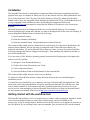
To convert a model in the .dae format to the .geom format, click the Voxelize CAD button and then use
the file chooser to select your .dae file. Upon selecting the file, the dialog box shown in Figure 2 will
appear. In this dialog box, the Resolution field sets the size in meters of each voxel in the .geom file
that will be created. Each such voxel will encompass a cube with sides of the length indicated in the
Resolution field. Your .geom model may be padded with empty space on the left and right, front and
back, and top and bottom by filling in the +x and -x, +y and -y, and +z and -z padding fields
respectively. These fields add the indicated number of meters to the bounding box that encompasses the
.dae model.
Figure 2. The NetwoRCSim voxelization dialog.
When you have entered the desired parameters into each field of the dialog, click the Convert button to
generate your .geom file. The name of the file that is generated will be the name of your .dae file
3
followed by the .geom extension. This file will be located in the same directory as the .dae file that was
converted. A second file is also created. This file has the name of the .dae file followed by the .mtl
extension, and it contains the electromagnetic properties of the materials that were discovered in
your .dae model. The default electromagnetic properties are thin glass for materials that are transparent
and metal for materials that are opaque.
2) Assign electromagnetic properties to your materials.
If the default assignment of materials is not acceptable for your simulation study, then you may change
the properties of those materials and then rerun the conversion from step 1 with the new material
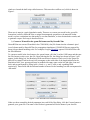
definitions. The first step in changing your material properties is to view your new .geom file. To do
this, click the Create study button and then use the file chooser to select the .geom file that was created
in step 1 above. This will launch the visualization tool, which is shown in Figure 3. Instructions for
using the visualization tool are the section titled “vis” in the table of contents. Each material in your
model is color coded, and the name of the material pointed at by the mouse is shown in the the upper
left corner of the display.
Figure 3. The NetwoRCSim visualization tool.
To create new electromagnetic properties for the materials, keep the visualization window open and
click the Manage materials button in the workflow tool. Then use the file chooser to select the .mtl file
that was created by the conversion tool in step 1 above. This will launch the material management
dialog that is shown in Figure 4.
4
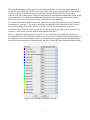
The material management dialog shows, on its left, the name and color of each material appearing in
the .dae file from which this .mtl file was created. On the right are drop down menus that may be used
to select from a list of predefined types of materials. These predefined materials include water,
concrete, soils, and a many others. Using the visualization tool and material management dialog, assign
to each material in your model a predefined material type from the drop down menu. When you are
down, click Save to save your choices the the .mtl file that you are managing.
To use these new material definitions in your .geom file, you must regenerate that .geom file using the
conversion tool from step 1. The steps for doing this are identical to those described in step 1 except
that you must change the materials model. To do this, click the Choose materials button in the
conversion dialog. Then use the file chooser to select the .mtl file that you have just saved. Now click
Convert to create a new .geom file with the new material definitions.
This new .geom file overwrites the old .geom file. A new .mtl file is also created that contains your
new material choices. This .mtl file overwrites your old .mtl file. Note that the material names shown in
the visualization tool do not change. However, if you load the new .mtl file into the material manager,
you will see your assignment of materials in the .dae file to NetworRCSIM's predefined material types.
Figure 4. The NetwoRCSim material manager.
5
3) Create a simulation study.
Click Create study in the workflow tool and then choose the .geom file that you want to use for your
simulation. This launches the visualization application, with which a transmitter can be placed into
your 3D model by clicking on a position in the model with your mouse. You may also choose the
carrier frequency of the transmitter by using the 'q' and 'z' keys (see the instructions in the “vis”
section). Placing the transmitter creates a .stdy file that describes the transmitter's location, frequency,
and other information necessary for a propagation simulation. The name of the .stdy file is displayed in
the text box that accompanies the visualization tool.
4) Run the simulation study.
Click Simulate in the workflow tool and then choose the .stdy file created in step 3. This launches the
simulation, which may take several minutes to finish. Its progress is reported in the text box that
appears when the simulation begins.
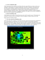
5) View the result of the simulation study.
Click View study in the workflow tool and then choose the .stdy file that was used for the simulation in
step 4. This launches the visualization tool to show the 3D path-loss data and delay spread data
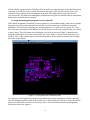
generated by the simulator. Figure 5 shows the path-loss from of a simulation study that uses the model
shown in Figure 3 with a 900 MHz transmitter and the default assignment of electromagnetic properties
to materials. The transmitter's location is visible as the bright spot near the center of the view.
Figure 5. Viewing the simulation output in the NetwoRCSim visualization tool.
6
6) Generate a report.
Click Write report and then choose the .stdy file that you viewed in step 5. This creates an HTML
document showing the 3D path-loss data, delay spread data, and the parameters used by the simulator
to create this data. The report generator lets you select the axis in the 3D model along which path-loss
and delay spread data will be displayed (e.g., choosing the z-axis will create maps showing the x-y
plane). The reporting dialog is shown in Figure 6.
Figure 6. The NetwoRCSim report generation form.
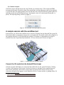
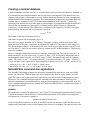
A sample session with the workflow tool
In this section you will use the workflow tool to convert a 3D model into the NetwoRCSim .geom file
format and conduct a propagation study for the converted model. The model used for this example is in
the examples directory of your NetwoRCSim package. This model of a hypothetical city block is
available from the Google SketchUp Warehouse1. A view of this model is shown in Figure 7.
Figure 7. A rendering of the city block model.
Convert the 3D model into the NetwoRCSim format
Click the Voxelize CAD button to convert the COLLADA file into the .geom file format. Clicking
Voxelize CAD launches a file chooser. Use this file chooser to navigate to the examples directory,
select the file cidade.dae, and click the Convert button at the bottom of the file chooser. In the
conversion dialog box that appears, set the Resolution field to 5 meters and the +z padding field to 50
1 Cidade, City 2.0. http://sketchup.google.com/3dwarehouse/details?
mid=33f14114ab35156b9f35c9921640ef78&ct=mdsa&prevstart=0
7
meters. Leave the other fields at their default values and click Convert at the bottom of the conversion
dialog. As the conversion progresses you will see a sequence of messages detailing each step of the
conversion process. When this is finished you will see the message './collada finished'. Click Ok when
this appears. The conversion creates a file called cidade.dae.geom in the examples directory.
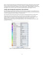
Assign electromagnetic properties to the materials
Press the Manage materials button and then use the file chooser to navigate to the examples directory
and choose the file cidade.dae.geom.mtl. In the material management dialog, use the drop down menu
to make the assignments shown in Figure 8. Then press Save.
Now repeat the steps from the previous section, but before converting the model, clock the button
Choose materials in the conversion dialog. Use the file chooser that appears to select the file
cidade.dae.geom.mtl. Then press the Convert button at the bottom of the conversion dialog. Once
again, you will see a sequence of messages describing the conversion process and a file
cidade.dae.geom will be created in the examples directory. This is the file that you will use in your
propagation simulation.
Figure 8. Assigning materials to the cidade.dae.geom model.
8
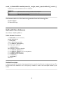
Placing the transmitter in the 3D model
To place a transmitter into the model, click the Create study button, use the file chooser to navigate to
the examples directory, and select the file cidade.dae.geom. This starts the visualization application,
which shows the model in two dimensional slices. The default view shows the x-y plane. You can go
up the z-axis by scrolling up with your mouse wheel or pressing the 'w' key. You can go down the zaxis by scrolling down with your mouse wheel or pressing the 's' key. The current position of your
mouse pointer in the model is shown in the upper left corner of the display.
Place the transmitter in the park behind the L-shaped building at the center of the city block. To do this,
scroll or press 's' until the z-coordinate of your mouse is 5, and then move the mouse until the display
shows the coordinate 355.163, 364.513, 5. This is where in Figure 9 you see a pink square. Now press
the left mouse button or the 'x' key. This creates the same pink square in your model to show the
location of the transmitter you have just placed and creates a .stdy file called cidade.dae.geom-1.stdy in
the examples directory. The .stdy file describes the transmitter position, frequency, and other
information used by the propagation simulator. Click on the 'X' in the corner of the visualization
window to close it and then press 'Ok' when the dialog saying './vis finished.' appears.
Figure 9. Placing a transmitter in the 3D model.
9
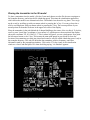
Running the simulator, visualizing the output, and generating a report
To run the simulation, click the Simulate button in the workflow tool and then use the file chooser to
select the file cidade.dae.geom-1.stdy, which was created when you placed the transmitter. This starts
the simulation. Its execution time can vary from seconds to hours, depending on the size of your model
and the processing power of your computer. In general, smaller models are simulated more quickly
than larger models, and computers with more processors (or cores) and more memory need less time to
run a simulation. The model used in this example should take about 12 minutes to simulate using a
single core computer, and less time if you have a license file and multiple processors or cores. When
the simulation is complete, you will be shown a message saying './rcsim finished'. Click Ok to continue.
The product of the simulation is a file called cidade.dae.geom-1.stdy.pdb that contains the strength of
the signal received at each voxel in the 3D model. The contents of this file can be visualized using the
visualization and report tools. To explore the signal database interactively, select View study and then
choose the .stdy file that was used to execute the simulation. This shows path-loss data in 2D slices. As
before, you can navigate along the z-axis by using the mouse wheel and the 'w and 's' keys. The view in
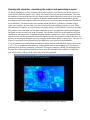
Figure 10 shows path-loss at ground-level; the bright spot is the location of the transmitter.
You can generate a report describing the simulator settings and showing path-loss maps for each of the
z- (or x- or y-) coordinates in the model by clicking Write report in the workflow tool. The report is
generated in the directory containing your model. This report comprises a HTML file and image files
for each slice of the signal data along your chosen axis. The NetwoRCSim workflow tool launches
your web browser to show you the report after it has been generated.
Figure 10. Viewing the path-loss data generated by the simulator.
10
Creating a material database
A material database is a plain text file (i.e., it can be edited with a text editor like Windows Notepad, or
vi or emacs) that ends with the extension .mtl has one line for each material. Each material has a one
character code, a name (without spaces), a color used for displaying the material in the vis application,
and the material's electromagnetic properties. The electromagnetic properties are the relative dielectric
constant, the two parameters of the ITU recommended attenuation model (see Ref. 7), and a flag
indicating if the material allows a radio signal to pass through it. If propagation through the material is
allowed, then the attenuation of the signal is calculated from the relative dielectric constant and
conductivity  of the material. The conductivity is a function of the frequency f in GHz of the signal
passing through the material and two parameters c and d as
σ=c f d S / m
The format of each line in the material file is
code name red green blue propagation_flag k c d
The code is any single, printable ASCII character. The name is a string without white-space. Red,
green, and blue are the color components for this material; each color component is in the range 0 to
255. The propagation flag is 1 if the material will allow a radio wave to pass through it and 0 if it will
not. The items k, c, and d are the relative dielectric constant and ITU model parameters. The line may
end with a comment.
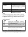
Below is a sample database that contains two materials: water and wood. The code for water is '!', its
name is material1, its color is blue (red = 0, green = 0, blue = 255), it will pass a radio signal, and its
electromagnetic model has k=80, c=0.574911, and d=1.16991. The material ends with the comment
'water'. The code for wood '”', it is named material0, is colored brown (red = 222, green = 184, blue =
135), it will pass a radio signal, and its electromagnetic properties are k=1.99, c=0.0047, and d=1.0718.
! material1 0 0 255 1 80 0.574911 1.16991 water
" material0 222 184 135 1 1.99 0.0047 1.0718 wood
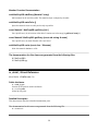
NetwoRCSim command-line applications
The NetwoRCSim package contains four proprietary command-line applications; these are collada,
params, vis, and rcsim. There are three open source applications; these are report, matdb_info, and
getpl. The source code for the open source applications is located in the src/examples and src/report
directories. The command-line applications are intended to facilitate automation, allowing you to
perform comprehensive simulation studies by using scripting languages or other automation tools. All
of the command-line applications are located in the networcs-platform folder. A detailed description of
each application follows.
params
This application calculates the parameters c and d of the ITU recommended attenuation model (see Ref.
7) given the material's relative dielectric constant and measurements of the dielectric loss tangent at
two frequencies. The syntax for params is
params k f1 tand1 f2 tand2 trials
where k is the relative dielectric constant, f1 and tand1 are the first frequency in Hz and dielectric loss
tangent, and f2 and tand2 are the second frequency and dielectric loss tangent. The optional trials is the
11
number of initial conditions to try when seeking a solution (the default is 100,000 and this should be
sufficient in most cases). The outputs of params are the conductivity values s1 and s2 calculated with
the discovered values of c and d, the expected values for s1 and s2 given the supplied dielectric loss
tangents, the L1 norm of the solution error (i.e., the difference between actual and expected values of
s1 and s2), and the values of c and d that were discovered.
matdb_info
The matdb_info application gives a summary description of a .geom file. The matdb_info application is
run with the command
matdb_info filename [freq]
where filename is a model in the .geom file format and freq is an optional frequency in Hz at which to
calculate the material properties. The default frequency for these calculations is 900 MHz. The
matdb_info program lists the materials appearing in the model and their properties, the dimensions of
the model, and a count of the voxels in total and by type.
rcsim
The rcsim application calculates path-loss, maximum delay spread, and root-mean-square delay spread
(see Ref. 8, pgs. 551-552) for a transmitter placed inside of a 3D model. The rcsim application is run
with the command
rcsim filename
where filename is a .stdy file that provides rcsim with the name of the .geom file, the location of the
transmitter in that geometry, the name to give to the signal database that rcsim creates, the frequency of
the transmitter, and other parameters for controlling precision and execution time. The .stdy file may be
created with the vis application or manually using a text editor (e.g., with Notepad on Windows, or vi
or emacs on Linux). A .stdy file has six lines, as shown in this example:
geom_file "/home/jim/NetwoRCSim/examples/cidade.dae.geom"
pwr_file "/home/jim/NetwoRCSim/examples/cidade.dae.geom-1.stdy.pdb"
tx 355.163 364.513 5
rxmin -95
freq 9e+08
The line beginning with geom_file tells rcsim the name of the 3D model in which the transmitter is
located. The line beginning with pwr_file to tell rcsim the name of the signal database it should create.
If this file with this name already exists, then it will be overwritten by rcsim and the original file will be
lost!
The line beginning with tx tells rcsim the location of the transmitter. The coordinates following tx are
the x,y,z location of the transmitter in the coordinate system of the 3D model.
The line beginning with rxmin gives the power level, relative to the transmitter output power, below
which the receiver is unable to process the received signal. This is expressed in dB power absorbed by
an omni-directional antennae relative to the power output of the transmitter. If, for example, the
transmitter output is 1 mW (0 dBm) and the receiver can tolerate 95 dBm of path-loss then the rxmin
value is -95. Similarly, if the output power of the transmitter is 1 W (0 dB) and the receiver can
tolerate 95 dB of path-loss, then rxmin is -95. But the same receiver listening to a 10 W (10 dB)
transmitter can tolerate 105 dB of path-loss, and so rxmin is -105.
12
The rxmin value is used in two ways. First, it is used as the stopping criteria for the simulation: when
every voxel experiences a path-loss less than rxmin the simulation terminates. Second, rxmin is used to
calculate the maximum delay spread (see Ref. 8). The delay spread calculation at a voxel starts when
the power level first exceeds rxmin and ends at the last instant that the power level is again below
rxmin.
The last line in the file, which begins with freq, is the frequency of the transmitter in Hertz.
report
The report application creates a radio coverage report in the form of an HTML document placed in the
directory that contains the .stdy file given to the report application. The report program is run with the
command
report filename axis
The filename is the name of a .stdy file processed by the rcsim application. The axis argument is 'x', 'y',
or 'z' and tells report which axis of the model to look along when taking its slices: 'x' looks at the model
straight on, 'y' from its left side, and 'z' from above. To illustrate, the command
report cidade.dae.geom-1.stdy z
generates a report from the simulation study used in the example, generating path-loss maps for each
slice along the z-axis.
getpl
The getpl application prints the path-loss at a specific point in a 3D model. The getpl program is run
with the command
getpl filename x y z [--raw] [ --grid ]
The first four arguments are the name of a signal database and the location at which to get the pathloss. The '--raw' and '--grid' arguments are optional. The '--raw' argument gets the unprocessed estimate
of the potential at that location. If the '--grid' argument is omitted, then the location is in model
coordinates. Otherwise the location is in voxel coordinates. To illustrate, the command
getpl cidade.dae.geom-1.stdy.pdb 360 325 5
calculates the path-loss for a receiver located at 360, 325, 5 meters using the signal database
cidade.dae.geom-1.stdy.pdb.
vis
The vis application is used to visualize propagation geometries and path-loss maps and to place
transmitters into a 3D model. The vis tools is started with the command
vis filename
where filename is a .stdy file or .geom file. The vis application is controlled with the keyboard and
mouse as described in the table below. The viewing window shows 2D slices of the 3D model. The
upper left corner of the display shows the model coordinate pointed at by the mouse, the path-loss (if
available) at that coordinate, the frequency of the transmitter, and the name of the material at that
location.
13
Key or action
Effect
Scroll the mouse up or press 'w'
Move up the viewing axis.
Scroll the mouse down or press 's'
Move down the viewing axis.
Left click or press 'x'
Place a transmitter at the location pointed at by the mouse and using
the frequency shown at the top of the display. This creates .stdy file
for simulating the transmitter at that location. The name of this file
is shown in the text box that accompanies the display.
Press the mouse wheel while scrolling up Increase the transmitter frequency.
or press 'q'
Press the mouse wheel while scrolling
down or press 'z'
Decrease the transmitter frequency.
Right click or press 'a'
Change the viewing axis.
Press 'm'
Change the data that is displayed from path-loss to rms delay spread
to maximum delay spread and back to path-loss.
collada
The collada application converts a polygon-based model in the COLLADA (.dae, see Ref. 6) file
format to a voxel-based model in the .geom file format. This conversion is done with the six-separating
algorithm described in Ref. 5. The COLLADA file format is exported by most 3D modeling tools, and
the collada application should permit the majority of models created with those tools to be used for
radio propagation simulations. The collada application is invoked with the command
collada [options] filename
where filename is the name of the COLLADA file to convert and [options] may be zero of more of the
options listed in the table below.
Option
Effect
size <meters>
Use voxels of size <meters> when converting the model. The default size is 1 m.
+x <meters>
This pads the “right” side of the model by adding <meters> meters to the positive xaxis edge. This space will be filled with air. The default is to add zero meters.
-x <meters>
As with +x, but pad the “left” side of the model.
+y <meters>
This pads the “front” side of the model by adding <meters> meters to the positive yaxis edge. This space will be filled with air. The default is to add zero meters.
-y <meters>
As with +y, but pad the “back” side of the model.
+z <meters>
This pads the “top” of the model by adding <meters> meters to the positive z-axis
edge. This space will be filled with air. The default is to add zero meters.
-z <meters>
As with +z, but pad the “bottom” of the model.
pad <meters>
Same effect as calling collada with the options +x <meters> -x <meters> +y
<meters> -y <meters> +z <meters> -z <meters>.
materials <filename>
Use the materials database <filename> when converting the model.
The collada application processes meshes comprising polylist, polygons, and triangles elements. If a
14
materials database is provided, then the name of the material bound to a polygon will be used to find
that polygon's electromagnetic properties in the materials database. If a materials database is not
provided, or if the material is not found, then collada uses a default value for the polygon's
electromagnetic properties. If the polygon's material is bound to an effect that has a transparency or
transparent element indicating some transparency, then the default material for that polygon is air (i.e.,
free space). Otherwise the default material is an ideal reflector (i.e., a perfectly conducting metal).
Transparency for this test is if the alpha component of the transparent element is less than one or the
transparency element is greater than zero.
To illustrate use of the collada application, the command
collada size 5 +z 50 cidade.dae
creates the .geom file used in the example simulation study and the .mtl file that contains the default
values for the electromagnetic properties for the materials in that model.
The C++ API for accessing geometry, material, and signal data
The application programming interface (API) for the C++ programming language lets end-users write
applications that use the NetwoRCSim geometry and signal databases and simulation study files. This
API is packaged as source code that may be compiled for your their particular development tools. The
source code should be compatible with most C++ compilers. Also included is source code for the getpl,
matdb_info and report applications. These applications provide examples of how to use the API.
The API consists of five classes and a handful of utility functions. The classes are the MaterialDB class
for accessing and creating 3D models (.geom files), the SignalDB class for accessing and creating
signal databases (.pdb files), the MatPropDB and Material classes for accessing tables of material
properties, and the SimParams class for reading and writing .stdy files. The utility functions support
these classes. Documentation for the C++ API is in the appendix of this document. The source code is
located in the src directory of the NetwoRCSim package.
Integration with NS3
The NetwoRCSim propagation simulator may be used as a propagation module for the NS3 network
simulator. This open source simulation tools is widely used for research, and is available online at
www.nsnam.org. The NS3 module for rcsim is located in the src/examples/ns3 directory of the
NetwoRCSim package. In the directory src/examples/ns3 is a directory called rcsim. Copy this
directory to the src directory of the NS3 simulator. Then reconfigure and rebuild the NS3 modules.
This will automatically include the NetwoRCSim module into your NS3 simulator under the module
name rcsim.
For example, if you have a new copy of NS3, are at the root of your NS3 source tree, are using version
of NS3, and the path to the root of your NetwoRCSim package is NetwoRCSim then the following set
of commands will build NS3 with the rcsim propagation module.
1. cp -r NetwoRCSim/src/ns3/rcsim ns3-version/src
2. ./build.py
To use the rcsim module, you must have the networcs-platform directory in your executable path. The
propagation module works as follows. When the NS3 simulator requests a path-loss calculation from
transmitter Tx to receiver Rx, it first looks into a cache directory for a signal database describing
15
transmitter Tx. The directory that is used to cache signal databases is an attribute of the rcsim
propagation module; its default value is to use the current directory (i.e., '.'). If a signal database for Tx
is found, the path-loss data for Rx is extracted from that database and returned.
If a signal database is not found, then the rcsim simulator is executed for the transmitter Tx. The
frequency that is used for this simulation is an attribute of the rcsim propagation module; its default
value is 900 MHz. Likewise, the .geom file that is used for the simulation is an attribute of the
propagation model; its default value is 'model.geom'. The .geom file must be located in the cache
directory. The signal database generated by the rcsim simulation is placed into the cache and the pathloss for Rx is returned.
In the examples directory of the rcsim propagation module, you will find two sample NS3 programs.
These demonstrate the use of the python and C++ API's for the rcsim propagation module. When you
run these examples, recall that they must be able to locate the cache directory. This requires that you
run the examples from the example directory, which contains the cache, or that you change the
examples to use the absolute path to the cache directory.
The advantage of owning a license
The free version of NetwoRCSim has all of the features described in this manual. Some of your
electromagnetic simulations, however, may be quite time consuming. By installing a license, you
enable the rcsim, params, and collada applications to exploit all of the cores in a multicore computer
and all of the processors in a shared memory multiprocessor computer. By purchasing and installing a
license, you automatically enable this parallel computing capability.
The parallel efficiency of the rcsim and params applications is close to 95%, and you can expect the
execution time of these applications to be reduced in proportion to the number of processors and cores
in your computer. For example, two cores will halve the execution time and four will quarter it. The
collada application is not quite as efficient in this respect, but you should see a reduction in execution
time for models with large numbers of polygons.
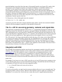
To illustrate the benefits of using multiple cores and processors, the table below shows execution times
for the params, collada, and rcsim applications using from 1 to 4 cores of a 4 core computer equipped
with 4 GB of RAM. The number of cores used by NetwoRCSim is controlled by setting the
OMP_NUM_THREADS environment variable. By default, all of the available cores and processors are
used.
Execution time vs. number of cores used
Application
Note
1 core
2 cores
3 cores
4 cores
params
100,000 trials
14 seconds
7.5 seconds
4.9 seconds
3.7 seconds
collada
2,879,514 polygons to
23,429,835 cells
20 seconds
17 seconds
15 seconds
14 seconds
rcsim
634,392 cells
284 seconds
148 seconds
96 seconds
75 seconds
16
References and bibliography
1. J. Nutaro, P.T. Kuruganti, R. Jammalamadaka, T. Tinoco, and V. Protopopescu. An Event
Driven, Simplified TLM Method for Predicting Path-Loss in Cluttered Environments. IEEE
Transactions on Antennas and Propagation, Vol. 56, No. 1, pp. 189-198, January 2008.
2. Nutaro, James; Kuruganti, Phani Teja, Fast, Accurate RF Propagation Modeling and Simulation
Tool for Highly Cluttered Environments, IEEE Military Communications Conference, 2007
(MILCOM 2007), pp.1-7, 29-31 Oct. 2007
3. James Nutaro. A discrete event method for wave simulation. ACM Transactions on Modeling
and Computer Simulation, 16(2):174-195, 2006.
4. Phani Teja Kuruganti and James Nutaro. A Comparative Study of Wireless Propagation
Simulation Methodologies: Ray Tracing, FDTD, and Event Based TLM. In the Proceedings of
the 2006 Huntsville Simulation Conference, Huntsville, Alabama, USA, October 2006.
5. Jian Huang, Roni Yagel, Vassily Filippov , Yair Kurzion. An accurate method for voxelizing
polygon meshes. IEEE Symposium on Volume Visualization, pp. 119-126, October 1998.
6. COLLADA – Digital Asset Schema Release 1.5.0 Specification. Editors Mark Barnes and Ellen
Levy Finch. April 2008.
7. Recommendation ITU-R P.1238-7 (02/2012). Propagation data and prediction methods for the
planning of indoor radio communication systems and radio local area networks in the frequency
range 900 MHz to 100 GHz . Online at http://www.itu.int/rec/R-REC-P.1238-7-201202-I/en
8. William H. Tranter, K. Sam Shanmugan, Theodore S. Rappaport, and Kurt L. Kosbar.
Principles of Communication Systems Simulation with Wireless Applications. Pearson
Education, Inc. 2004.
17
Appendix A. The C++ API.
Table of Contents
Table of contents
Class Index
Class List
Here are the classes, structs, unions and interfaces with brief descriptions:
coord_d_t ..............................................................................................................................................18
coord_t ..................................................................................................................................................19
FileException ........................................................................................................................................20
Material ................................................................................................................................................21
MaterialDB ...........................................................................................................................................22
MatPropDB ..........................................................................................................................................25
rx_detail_t ............................................................................................................................................26
SignalDB ...............................................................................................................................................27
SimParams ...........................................................................................................................................29
Class Documentation
coord_d_t Struct Reference
#include <data_types.h>
Public Member Functions
1
2
3
coord_d_t (double x, double y, double z)
bool operator== (const coord_d_t &b) const
bool operator!= (const coord_d_t &b) const
Public Attributes
4
5
6
double x
double y
double z
Detailed Description
Coordinate in the real-world (native) coordinate system of the 3D model.
18
Member Function Documentation
bool coord_d_t::operator== (const coord_d_t & b) const [inline]
Two coordinates are equal if they refer to the same point.
The documentation for this struct was generated from the following file:
7 data_types.h
coord_t Struct Reference
#include <data_types.h>
Public Member Functions
8
9
10
11
12
coord_t ()
coord_t (short int x, short int y, short int z)
bool inside_extent (const coord_t &other) const
bool operator== (const coord_t &b) const
bool operator!= (const coord_t &b) const
Public Attributes
13 short int x
14 short int y
15 short int z
Detailed Description
Coordinate in the voxel coordinate system.
Constructor & Destructor Documentation
coord_t::coord_t () [inline]
Default constructor does nothing.
coord_t::coord_t (short int x, short int y, short int z) [inline]
Constructor
19
Member Function Documentation
bool coord_t::inside_extent (const coord_t & other) const [inline]
Test if this coordinate is inside the specified extents. The coordinate is in the interior if on each axis it is not
less than zero and not more than the extent minus one.
bool coord_t::operator== (const coord_t & b) const [inline]
Two coordinates are equal if they refer to the same point.
The documentation for this struct was generated from the following file:
16 data_types.h
FileException Class Reference
#include <data_types.h>
Public Member Functions
17 FileException (std::string file_name, std::string msg="", int err_code=-1)
18 std::string getFileName () const
Get the file name.
19 std::string getErrorMsg () const
Get the error message.
20 int getErrorCode () const
Get the errno error code.
Detailed Description
A FileException is thrown when there is a problem accessing a file.
Constructor & Destructor Documentation
FileException::FileException (std::string file_name, std::string msg = "", int err_code =
-1) [inline]
Arguments are the file being accessed, a message to display, and the errno error number if appropriate (use
-1 to indicate no errno code).
The documentation for this class was generated from the following file:
21 data_types.h
20
Material Class Reference
#include <Material.h>
Public Types
22 enum Type { FREE_SPACE, IDEAL_REFLECTOR }
Public Member Functions
23
24
25
26
27
28
29
30
31
32
33
34
35
36
37
38
39
40
41
42
43
44
45
Material (Type type=FREE_SPACE, float freq=900.0E6)
Material (const Material &src)
float Z () const
float gain () const
float alpha () const
bool prop () const
int red () const
void red (int r)
int green () const
void green (int g)
int blue () const
void blue (int b)
const std::string & name () const
void name (const std::string &name)
void name (const char *name)
const std::string & extra () const
char code () const
void code (char code)
double rel_k () const
void freq (float f, float dx=1.0f)
void read (const std::string &str)
std::string write () const
~Material ()
Destructor.
Detailed Description
This class has the electromagnetic properties of a specific material.
Member Function Documentation
void Material::freq (float f, float dx = 1.0f)
Calculate resistance and attenuation per voxel for the given frequency and grid resolution
void Material::read (const std::string & str)
Load a material from the supplied string.
21
std::string Material::write () const
Write the material to a string and return the string.
The documentation for this class was generated from the following files:
46 Material.h
47 Material.cpp
MaterialDB Class Reference
#include <MaterialDB.h>
Public Member Functions
48
49
50
51
52
53
54
55
56
57
58
59
60
61
62
63
64
65
MaterialDB (const char *filename, double dx, coord_t extent, coord_d_t origin)
MaterialDB (std::string filename, float freq=900.0E6)
std::string getFilename () const
coord_t getExtents ()
const Material * getProperty (char code)
const char * getMaterialName (char code)
char getCode (const std::string &name)
int getMaterialCodeCount ()
char getCode (const coord_t &c)
char addMaterial (Material *material)
void setCode (char code, const coord_t &c)
bool insideExtent (const coord_t &c)
double getResolution ()
coord_d_t getOrigin ()
coord_t getPoint (const coord_d_t &orig)
coord_d_t getPoint (const coord_t &grid)
void save ()
~MaterialDB ()
Static Public Member Functions
66 static coord_t translate (coord_d_t origin, coord_d_t pos, double dx)
67 static coord_d_t translate (coord_d_t origin, coord_t pos, double dx)
Detailed Description
This class is used to read and write 3D models in the .geom file format.
22
Constructor & Destructor Documentation
MaterialDB::MaterialDB (const char * filename, double dx, coord_t extent, coord_d_t
origin)
Create a new model that is filled with air.
Parameters:
filename
dx
extent
origin
The name of the file to create. Any existing file will be overwritten.
The size of a voxel in meters.
The dimensions of the model in voxels.
The real-world location of the 0,0,0 voxel.
MaterialDB::MaterialDB (std::string filename, float freq = 900.0E6)
Load an existing model. Throws a FileException if the model can not be opened. The material models are
adjusted to match the supplied frequency.
Parameters:
filename
frequency
The name of the file to open.
Frequency in Hertz for calculating the material properties.
MaterialDB::~MaterialDB ()
Destructor. Changes that have not been saved will be lost.
Member Function Documentation
char MaterialDB::addMaterial (Material * material)
Add a material to the model and return the code for this material. If a material with the same name already
exists then its properties are replaced with the supplied properties. The material object is adopted by the
MaterialDB object.
char MaterialDB::getCode (const std::string & name)
Get the code of a material for the supplied name. Returns getMaterialCodeCount if the name is not found.
char MaterialDB::getCode (const coord_t & c)
Get the material code located at the given voxel.
coord_t MaterialDB::getExtents () [inline]
Get the x, y, and z extents of the model in voxels.
std::string MaterialDB::getFilename () const [inline]
Get the filename for the model.
int MaterialDB::getMaterialCodeCount () [inline]
Get the number of material codes that appear in the model. Material code numbers are from 0 to
getMaterialCodeCount()-1.
23
const char* MaterialDB::getMaterialName (char code) [inline]
Get the name of the material that has the given code.
coord_d_t MaterialDB::getOrigin () [inline]
Get the model's origin in the its native coordinate system.
coord_t MaterialDB::getPoint (const coord_d_t & orig)
Get the voxel that contains the given native coordinate.
coord_d_t MaterialDB::getPoint (const coord_t & grid)
Get native coordinate at the center of the given voxel.
const Material* MaterialDB::getProperty (char code) [inline]
Get the electro-magnetic properties associated with the material code.
Parameters:
code
A code for a material that is in the model.
double MaterialDB::getResolution () [inline]
Get the size of a voxel in meters.
bool MaterialDB::insideExtent (const coord_t & c) [inline]
Returns true if the point is inside of the model's bounding volume.
void MaterialDB::save ()
Write the model to disk if it has been modified.
Try to open the file for writing.
Write the material property data.
Write extents and the grid resolution.
Write the origin of the grid in original coordinates.
Write all of the grid codes.
void MaterialDB::setCode (char code, const coord_t & c)
Set the type of material at a voxel in the model.
coord_t MaterialDB::translate (coord_d_t origin, coord_d_t pos, double dx) [static]
Translate from native coordinates to voxel coordinates.
Parameters:
origin
pos
dx
The location of the voxel 0,0,0 in real-world coordinates.
The real-world location whose containing voxel we want to find.
The size of a voxel in meters.
24
coord_d_t MaterialDB::translate (coord_d_t origin, coord_t pos, double dx) [static]
Translate from voxel coordinates to native coordinates.
Parameters:
origin
pos
dx
The location of the voxel 0,0,0 in real-world coordinates.
The voxel whose real-world location we want to find.
The size of a voxel in meters.
The documentation for this class was generated from the following files:
68 MaterialDB.h
69 MaterialDB.cpp
MatPropDB Class Reference
#include <MatPropDB.h>
Public Member Functions
70 MatPropDB (const char *filename)
Load the materials file.
71 MatPropDB ()
Create a default materials table.
72 const Material * getFreeSpace ()
Get the free space material.
73 int getEntryCount ()
Get the number of entries in the table.
74
75
76
77
78
79
const Material * getEntry (int i)
const Material * getEntry (const std::string &name)
void addEntry (Material *entry)
void write (const char *filename)
void autoColor ()
~MatPropDB ()
Destructor.
Detailed Description
A material properties file contains electromagnetic data for materials. Each line has a single material type. The
first line must be the material to use for free space (or whatever is used for the unoccupied medium in your
model).
25
Member Function Documentation
void MatPropDB::addEntry (Material * entry)
Add a material to the end of the table. The material object is adopted by the table.
void MatPropDB::autoColor ()
Space the material colors as widely and evenly as possible.
const Material * MatPropDB::getEntry (int i)
Get a specific entry by its location in the table. Locations are in the range [0,getEntryCount()-1].
const Material* MatPropDB::getEntry (const std::string & name)
Get a specific entry by name. Returns null if not found.
void MatPropDB::write (const char * filename)
Write this material database to a file.
The documentation for this class was generated from the following files:
80 MatPropDB.h
81 MatPropDB.cpp
rx_detail_t Struct Reference
#include <SimParams.h>
Public Attributes
82 coord_d_t pos
Location of the point in model coordinates.
83 std::string label
A label for the point.
Detailed Description
This data structure describes a detailed measurement point.
The documentation for this struct was generated from the following file:
84 SimParams.h
26
SignalDB Class Reference
#include <SignalDB.h>
Public Member Functions
85 SignalDB (const char *filename, double dx, coord_t extent, coord_t tx_pos, float tx_freq, coord_d_t origin)
86 SignalDB (const char *filename, bool in_memory=false)
87 coord_t getTxPos () const
Get the voxel that contains the transmitter.
88 coord_t getExtents () const
Get the dimensions of the database in voxels.
89 float getTxFreq () const
Get the transmitter frequency in hertz.
90 float getRecord (coord_t pos, float *rms_ds=NULL, float *max_ds=NULL)
91 float getRecord (coord_d_t pos, float *rms_ds=NULL, float *max_ds=NULL)
92 coord_d_t getOrigin () const
Get the origin of the volume in real-world coordinates.
93 double getGridResolution () const
Get the size of a voxel in meters.
94
95
96
97
98
99
100
101
102
103
void writeRecord (float value, coord_t pos, float rms_ds=0.0f, float max_ds=0.0f)
float getRxPower (coord_t pos)
float getRxPower (coord_t pos, float freq)
float getRxPower (coord_d_t pos)
float getRxPower (coord_d_t pos, float freq)
float getRmsDelaySpread (coord_t pos)
float getRmsDelaySpread (coord_d_t pos)
float getMaxDelaySpread (coord_t pos)
float getMaxDelaySpread (coord_d_t pos)
~SignalDB ()
Close the database.
104 float calcVoltage (float p)
Static Public Member Functions
105 static float calcPowerLoss (float v, float freq, float dx)
106 static float calcVoltage (float p, float freq, float dx)
Detailed Description
This class is for reading from and writing to a signal database produced by the simulator.
Constructor & Destructor Documentation
SignalDB::SignalDB (const char * filename, double dx, coord_t extent, coord_t tx_pos,
float tx_freq, coord_d_t origin)
Create an empty database. The file that is created will overwrite any existing file with the same name.
27
Parameters:
filename
dx
extent
tx_pos
tx_freq
origin
Name of the file to create or overwrite.
Size of a voxel in meters.
Three dimensional volume contained in the signal database. The dimensions
are in voxels.
The voxel in which the transmitter is located.
Transmitter frequency in Hz.
Real-world location of the lower left corner of the volume.
SignalDB::SignalDB (const char * filename, bool in_memory = false)
This constructor opens an existing signal database. If in_memory is true, then the database will be loaded
into memory; if false, access is via the disk.
Member Function Documentation
float SignalDB::calcPowerLoss (float v, float freq, float dx) [static]
Calculate the pathloss in dB for a given potential, frequency, and grid resolution. Assumes a transmitter
voltage of 1.
Parameters:
v
freq
dx
The voltage level
The frequency in Hz
The grid resolution in meters.
float SignalDB::calcVoltage (float p, float freq, float dx) [static]
Calculate the potential for a given pathloss, frequency, and grid resolution. This assumes a transmitter power
of 0 dB.
Parameters:
p
freq
dx
The pathloss in dB
The frequency in Hz
The grid resolution in meters
float SignalDB::calcVoltage (float p)
Calculate potential using the frequency and resolution stored in this database.
float SignalDB::getRecord (coord_t pos, float * rms_ds = NULL, float * max_ds = NULL)
Get the maximum potential at a voxel. Also returns the rms delay spread and maximum delay spread if
rms_ds and max_ds are not NULL by writing this value to the supplied float.
float SignalDB::getRmsDelaySpread (coord_t pos)
Get the delay spread at a specific location. Units are in seconds.
float SignalDB::getRxPower (coord_t pos)
Get the pathloss for an isotropic antennae.
Parameters:
pos
The voxel containing the receiving antennae.
28
float SignalDB::getRxPower (coord_t pos, float freq)
Get the pathloss for an isotropic antennae adjusted for a frequency different from what was given to the
simulator. This will be accurate if the model contains only materials without frequency dependent
attenuation. It will be an approximation otherwise.
Parameters:
pos
freq
The voxel containing the receiving antennae.
The carrier frequency in Hertz.
float SignalDB::getRxPower (coord_d_t pos)
Get the pathloss for an isotropic antennae.
Parameters:
pos
The real-world location in meters of the receiving antennae.
float SignalDB::getRxPower (coord_d_t pos, float freq)
Get the pathloss for an isotropic antennae adjusted for a frequency different from what was used in the
simulation that generated this data set.
Parameters:
pos
freq
The real-world location in meters of the receiving antennae.
The carrier frequency in Hertz.
void SignalDB::writeRecord (float value, coord_t pos, float rms_ds = 0.0f, float
max_ds = 0.0f)
Write the potential and delay spread values at a voxel.
Parameters:
value
pos
rms_ds
max_ds
The maximum potential at the voxel.
The voxel itself.
The rms delay spread.
The maximum delay spread.
The documentation for this class was generated from the following files:
107SignalDB.h
108SignalDB.cpp
SimParams Class Reference
#include <SimParams.h>
Public Member Functions
109 SimParams (const char *filename)
110 coord_d_t getTxPos ()
Get the transmitter position in model coordinates.
29
111 std::string getMatDbFile ()
Get the filename for the geometry database.
112 std::string getPowerDBFile ()
Get the filename for the power and multipath database.
113 float getRxFloor ()
114 float getFreq ()
Get the transmitter frequency in Hz. Default is 900 MHz.
115 const std::vector< coord_d_t > & getJuncsToRecord () const
Get the vector of coordinates to record.
116 ~SimParams ()
Destructor.
Static Public Member Functions
117 static std::string createSetupFile (coord_d_t tx_pos, float tx_freq, std::string geom_file)
118 static void createSetupFile (coord_d_t tx_pos, float tx_freq, std::string geom_file, std::string stdy_file)
Detailed Description
This class is used to load and access the contents of a simulation setup file.
Constructor & Destructor Documentation
SimParams::SimParams (const char * filename)
Load the specified setup file. Throws a FileException if the file can not be loaded.
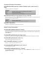
Member Function Documentation
static std::string SimParams::createSetupFile (coord_d_t tx_pos, float tx_freq,
std::string geom_file) [static]
Create a default setup file for a simulation with the transmitter at the given position in the given 3D model.
Returns the name of the setup file that was created.
static void SimParams::createSetupFile (coord_d_t tx_pos, float tx_freq, std::string
geom_file, std::string stdy_file) [static]
Create a setup file with the given filename. Overwrites any existing file.
float SimParams::getRxFloor () [inline]
Get the receiver sensitivity in dB. This is used for calculating multipath interference and for deciding when
to stop the simulation. The default value is -95 dB.
30
The documentation for this class was generated from the following files:
119SimParams.h
120SimParams.cpp
31