Download Basics of Image Processing and Analysis

Kota Miura
EMBL-CMCI course I
Basics of Image Processing and
Analysis
ver 2.1.1
Centre for Molecular & Cellular Imaging
EMBL Heidelberg
Abstract
Aim: students acquire basic knowledge and techniques for handling digital image data by interactively using ImageJ.
NOTE: this textbook was written using the Fiji distribution of ImageJ (IJ
ver 1.47n, JRE 1.6.0_45). Exercises are recommended to be done using Fiji
since most of plugins used in exercises are pre-installed in Fiji.
Many texts, images and exercises especially for chapter 1.3 and 1.4 were
converted from the textbook of Matlab Image Processing Course in MBL,
Woods Hall (which are originally from a book Digital Image Processing using
Matlab, Gonzalez et al, Prentice Hall). I thank Ivan Yudushkin for providing
me with the manual he used there. Deconvolution tutorial was written by
Alessandra Griffa and appears in this textbook with her kind acceptance
to do so. Figures on stack editing are drawn by Sébastien Toshi for his
course and appear in this textbook for his kind offer. I am pretty much
thankful to his figure and am impressed with the way he summarized all
the commands related to this. Sébastien Toshi also reviewed the article in
detail and made may suggestions to improve the text. I thank him a lot for
his effort.
This text is progressively edited. Please ask me when you want to distribute.
Compiled on: November 21, 2013
Copyright 2006 - 2013, Kota Miura (http://cmci.embl.de)
Contents
1.1
1.2
Basics of Basics . . . . . . . . . . . . . . . . . . . . . . . . . .
4
1.1.1
Digital image is a matrix of numbers . . . . . . . . . .
4
1.1.2
Image Bit-Depth . . . . . . . . . . . . . . . . . . . . .
7
1.1.3
Converting the bit-depth of an image . . . . . . . . .
10
1.1.4
Math functions . . . . . . . . . . . . . . . . . . . . . .
14
1.1.5
Image Math . . . . . . . . . . . . . . . . . . . . . . . .
17
1.1.6
RGB image . . . . . . . . . . . . . . . . . . . . . . . .
18
1.1.7
Look-Up Table . . . . . . . . . . . . . . . . . . . . . .
24
1.1.8
Image File Formats . . . . . . . . . . . . . . . . . . . .
27
1.1.9
Multidimensional data . . . . . . . . . . . . . . . . . .
29
1.1.10 Command Finder . . . . . . . . . . . . . . . . . . . . .
40
1.1.11 Visualization of Multidimensional Images . . . . . .
41
1.1.12 Resampling images (Shrinking and Enlarging) . . . .
47
1.1.13 ASSIGNMENTS . . . . . . . . . . . . . . . . . . . . .
50
Intensity . . . . . . . . . . . . . . . . . . . . . . . . . . . . . .
52
1.2.1
Histogram . . . . . . . . . . . . . . . . . . . . . . . . .
52
1.2.2
Region of Interest (ROI) . . . . . . . . . . . . . . . . .
55
1.2.3
Intensity Measurement . . . . . . . . . . . . . . . . . .
56
1.2.4
Image transformation: Enhancing Contrast . . . . . .
59
EMBL CMCI ImageJ Basic Course
1.2.5
1.4
1.5
Image correlation between two images: co-localization
plot . . . . . . . . . . . . . . . . . . . . . . . . . . . . .
61
ASSIGNMENTS . . . . . . . . . . . . . . . . . . . . .
62
Filtering . . . . . . . . . . . . . . . . . . . . . . . . . . . . . .
63
1.3.1
Convolution . . . . . . . . . . . . . . . . . . . . . . . .
63
1.3.2
Kernels . . . . . . . . . . . . . . . . . . . . . . . . . . .
67
1.3.3
Morphological Image Processing . . . . . . . . . . . .
72
1.3.4
Morphological processing: Opening and Closing . .
76
1.3.5
Morphological Image Processing: Gray Scale Images
77
1.3.6
Background Subtraction . . . . . . . . . . . . . . . . .
78
1.3.7
Other Functions: Fill holes, Skeltonize, Outline . . . .
80
1.3.8
Batch Processing Files . . . . . . . . . . . . . . . . . .
81
1.3.9
Fast Fourier Transform (FFT) of Image . . . . . . . . .
83
1.3.10 Frequency-domain Convolution . . . . . . . . . . . .
87
1.3.11 Frequency-domain Filtering . . . . . . . . . . . . . . .
90
1.3.12 ASSIGNMENTS . . . . . . . . . . . . . . . . . . . . .
94
Segmentation . . . . . . . . . . . . . . . . . . . . . . . . . . .
95
1.4.1
Thresholding . . . . . . . . . . . . . . . . . . . . . . .
95
1.4.2
Feature Extraction - Edge Detection . . . . . . . . . . 100
1.4.3
Morphological Watershed . . . . . . . . . . . . . . . . 103
1.4.4
Particle Analysis . . . . . . . . . . . . . . . . . . . . . 105
1.4.5
Machine Learning: Trainable Segmentation . . . . . . 108
1.4.6
ASSIGNMENTS . . . . . . . . . . . . . . . . . . . . . 112
1.2.6
1.3
CONTENTS
Analysis of Time Series
1.5.1
. . . . . . . . . . . . . . . . . . . . . 115
Difference Images . . . . . . . . . . . . . . . . . . . . . 115
2
EMBL CMCI ImageJ Basic Course
CONTENTS
1.5.2
Projection of Time Series . . . . . . . . . . . . . . . . . 116
1.5.3
Measurement of Intensity dynamics . . . . . . . . . . 117
1.5.4
Measurement of Movement Dynamics . . . . . . . . . 117
1.5.5
Kymographs . . . . . . . . . . . . . . . . . . . . . . . 118
1.5.6
Manual Tracking . . . . . . . . . . . . . . . . . . . . . 121
1.5.7
Automatic Tracking . . . . . . . . . . . . . . . . . . . 123
1.5.8
Summarizing the Tracking data . . . . . . . . . . . . . 129
1.5.9
ASSIGNMENTS . . . . . . . . . . . . . . . . . . . . . 132
References . . . . . . . . . . . . . . . . . . . . . . . . . . . . . . . . 133
1.6
Appendices . . . . . . . . . . . . . . . . . . . . . . . . . . . . 139
1.6.1
App.1 Header Structure and Image Files . . . . . . . 139
1.6.2
App.1.5 Installing Plug-In . . . . . . . . . . . . . . . . 140
1.6.3
App.1.75 List of accompanying PDF . . . . . . . . . . 141
1.6.4
App.2 Measurement Options . . . . . . . . . . . . . . 142
1.6.5
App.3 Edge Detection Principle
1.6.6
App.4 Particle Tracker manual . . . . . . . . . . . . . 149
1.6.7
App.5 Particle Analysis . . . . . . . . . . . . . . . . . 163
1.6.8
App.6 Image Processing and Analysis: software, script-
. . . . . . . . . . . . 147
ing language . . . . . . . . . . . . . . . . . . . . . . . . 165
1.6.9
App.7 Macro for Generating Striped images . . . . . 167
1.6.10 App.8 Deconvolution Exercise . . . . . . . . . . . . . 168
3
EMBL CMCI ImageJ Basic Course
1.1
1.1 Basics of Basics
Basics of Basics
Handling of digital images in scientific research requires knowledge on the
characteristics of digital images. A digital image translates to numbers and
is hence a quantitative signal by nature. In this section, we learn the very
basics of the numerical nature of digital images. Inappropriate handling
not only lowers the quality of your analysis, but it could also be possible
that your processing is considered as a "manipulation of data". For this latter point, please also refer to Rossner and Yamada (2004). There are some
limits on acceptable image processing to maintain the scientific validity.
Standards on scientific image processing could be found in "Digital Imaging: Ethics" by Cromey (2007).
1.1.1
Digital image is a matrix of numbers
A digital image we display on a computer screen is made up of pixels. We
can see individual pixel by zooming up the image using the magnifying
tool1 . Width and height of the image are defined by the number of pixels in
x and y directions. Each pixel has brightness, or intensity (or more strictly,
amplitude) somewhere between black and white represented as a number.
Within an image file saved in a computer hard disk, the intensity value
of each pixels are written. The value is converted to the grayness of that
pixel on monitor screen. We usually do not see these values, or numbers,
in the image displayed on monitor, but we could access these numbers in
the image file by converting the image file to a text file 2 .
Exercise 1.1.1-1
Conversion of image to a text file
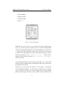
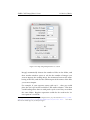
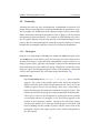
Make a new image by [File > New > Image...]. In dialog window, make a new image with the following parameters:
• name = test.txt
• type = 8bit
1
Zooming in / out of the image does not change the content of the image.
also possible in a limited way by moving the mouse pointer over the image and
checking the number indicated in ImageJ menu bar.
2 It’s
4
EMBL CMCI ImageJ Basic Course
1.1 Basics of Basics
• Fill with Black
• 10 pixel width
• 15 pixel height
• Slices = 1
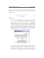
Figure 1.1 – New Image Dialog
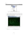
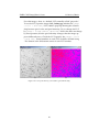
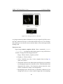
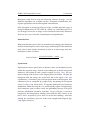
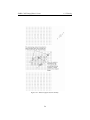
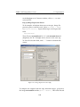
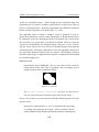
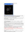
Clicking "OK", you will see a new window showing a black image
(Fig. 1.2). At the top of the window you can see the file dimension
("10 x 15"), bit-depth and the file size (I will explain these values later.
). Take the pen tool and draw some shape (what ever you want. If
you do not see anything drawn, then you need to change the color of
the pen to white by [Edit > Option > Colors...] and set Foreground Color to white). Then do [File > Save as > Text image]
and save the file.
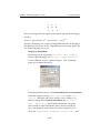
You will find that the name of the file ends with ".txt". Open File
Explorer (Win) or Finder (Mac) and double click the file. The file will
be opened in text editor.
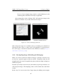
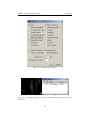
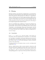
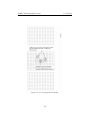
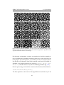
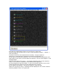
What you see now in the text editor is a "text image", a 2D matrix
of tab-delimited numbers. At the left most column in the example
(Fig. 1.3), there are only zeros. This corresponds to the left column
pixels in the image, where the color is black. In the middle in the
5
EMBL CMCI ImageJ Basic Course
1.1 Basics of Basics
example image, there are several "255". These are the white part of
the image. In the text image, edit one of the numbers (either 0 or 255)
and change to 100. Then save the file with a different name, such as
"temp.txt". Then in ImageJ open the file by [File > Import > Text
Image...]. You should see some difference in the image now. The
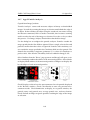
image now has a dark gray dot, not black nor white.
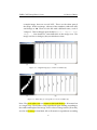
(a)
(b)
Figure 1.2 – A digital image (b) is a matrix of numbers (b).
(a)
(b)
Figure 1.3 – White line (a) corresponds to non-zero numbers (b).
Note: The pixel values are not written to the hard disk as a 2D matrix but
as a single array. The matrix is only reproduced upon loading according to
the width and height of the image. Pixel values of image stacks (3D or 4D),
are also in 1D array in hard disk. 3D or 4D matrix is reproduced according
6
EMBL CMCI ImageJ Basic Course
1.1 Basics of Basics
to additional information such as slice and channel number. Such information is written in the "header" region of the file, which precedes the "data"
region of the file where the 1D array of pixel array is contained. The header
structure depends on the file format, many such formats exist (the most
common are TIFF or BMP, we will see more in "file formats and header"
section).
1.1.2
Image Bit-Depth
Image file has a defined bit depth. You might have already heard terms
like "8-bit" or "16-bit" and these are the bit depth. 8-bit means that the grayscale of the image has 28 = 256 steps: in other words, the grayness between
black and white is divided into 256 steps. In the same way 16-bit translates
to 216 = 65536 steps, hence for 16-bit images one can assign gray-level to
pixels in a much more precise way; in other words "grayness resolution" is
higher.
Microscope images are generated mostly by CCD camera (or
something similar). CCD chip has a matrix of sensors. Each
sensor receives photons and converts the number of photons
to a value for a pixel at the corresponding position within the
image. Larger bit-depth enables more detailed conversion of
signal intensity (infinite steps) to pixel values (limited steps).
Why do we use "2n "? This is because computers code the information with
binary numbers. In binary the elementary units are called bits and there
only possible values are 0 and 1 (in the decimal system these units are called
digits and can take values from 0 to 9). Coding values with 8-bit means for
example that this value is represented as a 8 bit number, something like
"00001010" ( = 10 in decimal). Then the minimum value is = "00000000"
("0" in decimal) and the maximum is 11111111 ("255" in decimal). 8-bit image allows 256 scales for the grayness (using calculator application in your
computer, you could easily convert binary number into normal decimals
and vice versa). In case of 16-bit image, the scale is 216 so there are 65536
steps.
7
EMBL CMCI ImageJ Basic Course
1.1 Basics of Basics
We must not forget that the nature is continuous. In conventional mathematics (as you learn in school), a decimal point enables you to represent
infinite steps between 0 and 1. But by digitizing the nature we lose the ability to encode infinite steps such that 0.44 might be rounded to 0 and 0.56 to
1. Thus, the bit-depth limits the resolution of the analog to digital conversion (AD conversion). Higher bit depth generally allows higher resolution.
ImageJ has a high-bit-depth format called signed 32-bit floating point image. In all above cases with 8-bit and 16-bit, the pixel value is represented
in integer but floating-point type enables decimal points (real number) for
the pixel value such as "15.445". Though 32-bit floating point image can be
used for image calculation, many functions in ImageJ do not handle them
properly so cares should be taken when using this image format. If you
want to know more about the 32-bit format, read the following box (a bit
complicated; you could just pass through)
32 bit FLOATING POINT images utilizes efficient use of the
32 bits. Instead of using 32 bits to describe 4,294,967,296 integer
numbers, 23 bits are allocated to a fraction, 8 bits to an exponent, and 1 bit to a sign, as follows:
V = (−1) S ∗ 1.F ∗ 2 ( E − 127),
whereby:
S = Sign, uses 1 bit and can have 2 possible values
F = Fraction, uses 23 bits and can have 8,388,608 possible values
E = Exponent, uses 8 bits and can have 256 possible values
Practically speaking, this allows for an almost infinite number
of tones between level "0" and "1", more than 8 million tones
between level "1" and "2" and 128 tones between level "65,534"
and "65,535", much more in line with our human vision than a
32 bit integer image. Because of the infinitesimally small numbers that can be stored, the 32 bit floating point format allows
to store a virtually unlimited dynamic range. In other words,
32 bit floating point images can store a virtually unlimited dynamic range in a relatively compact way with more detail in the
8
EMBL CMCI ImageJ Basic Course
1.1 Basics of Basics
shadows than in the highlights and take up only twice the size
of 16 bits per channel images, saving memory and processing
power. A higher accuracy format allows for smoother dynamic
and tonal range compression.
(Quote from http://www.dpreview.com/learn/?/key=bits)
Guide Line for the Choice of Bit-Depth
In fluorescence microscopy, the choice of whether to use higher bit-depth
format depends on a balance among the intensity of excitation light, the
emision signal intensity, the sensitivity of photon detector, quantum efficiency3 and the gain. If the signal is bright enough then there would good
S/N that you could simply use a lower bit depth but if the signal is too
bright then you might need to use a higher bit depth just to avoid saturating the bits. This balancing could also be controlled by changing the gain
of the camera. In the end, the choice of bit depth depends on what type
of measurement you want to achieve. If you only need to determine the
shape of the target object (“segmentation”), you might not need a higher
bit depth image as you could try to adjust the imaging condition rather
than increasing the file size of the image. On the other hand, if you are trying to measure protein density, a higher bit depth allows you to have more
precise measurements so a larger bit-depth is recommended. A draw back
is that it takes longer time for data transferring as the bit-depth becomes
larger. This may in turn limits the time resolution of image sequences. The
balancing between imaging conditions and the type of analysis afterward
is very much coupled and should be thought well before your experiment.
More details on this discussion could be found in microscopy textbook such
as Pawley (2006).
The choice of bit depth depends on deals with noise. Here is an explanation
from Sébastien Tosi:
When minute details need to be preserved in both high and low
3 Quantum effeciency is a measure of proportion of photons converted to electric impluse. For example, QE of photographic film is ca. 10%, that of human eye is 20%. Recent
CCD allows 80%.
9
EMBL CMCI ImageJ Basic Course
1.1 Basics of Basics
intensity regions of a sample a large bit-depth is necessary to
ensure a good image quality. Indeed for low bit-depth if the signal level is adjusted to avoid saturation in the brightest regions
there is a high risk to end up coding the signal of the faintest regions over only very few bits, which has a very detrimental effect on the image quality. A large bit depth is hence necessary to
provide a fine slicing of the intensity range while provisioning
a sufficient headroom to avoid saturation and as such always
the safest option.
It can be mathematically derived that quantizing a continuous
signal to a finite number of levels induces an Additive White
(un-correlated) noise commonly called “quantization noise”. The
level of this noise source is conditioned by the number of levels
that are allowed (over the effective range of the signal). Depending on the image intrinsic noise (shot noise at a given photon regime) and the noises coming from the detector and the
amplifier electronics this noise can eventually be neglected. One
should always make sure that this noise source can be neglected
to avoid trashing valuable (available) information.
(personal communication, Sébastien Tosi)
1.1.3
Converting the bit-depth of an image
In many occasions, you might want to decrease the bit-depth of image simply to reduce the file size (16-bit file becomes half the file size when it is converted to 8-bit), or you might need to use certain algorithm that is available
only with 8-bit images (there are many such cases), or so on. In any case,
this will be a good experience for you to see the limitation of bit-depth.
Here, we focus on the conversion of a 16-bit image to an 8-bit image to
study its effect and associated possible errors.
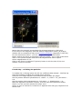
Exercise 1.1.3-1
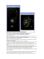
Let’s first open a 16-bit image from the sample. If you have the course
plugin installed, choose the menu item [EMBL > Samples > m51.tif].
Otherwise, if you have sample images saved in your local machine,
10
EMBL CMCI ImageJ Basic Course
1.1 Basics of Basics
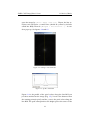
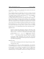
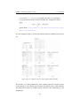
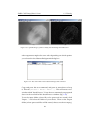
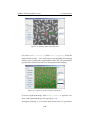
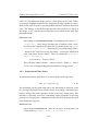
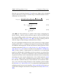
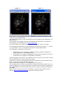
open the image by [File > Open > m51.tif]. Choose the line selection tool and draw a vertical line (should be yellow by default:
called line ROI). Then do [Analyze > Plot Profile...]. A window pops up. See figures 1.4 and 1.5.
Figure 1.4 – Setting a vertical line Roi.
Figure 1.5 – profile of that ROI
Figure 1.4 is the profile of the pixel values along the line ROI you
just have marked on the image (Fig. 1.5). X-axis is the distance from
the starting point (in pixel) and the y axis is the pixel value along the
line ROI. The peak corresponds to the bright spot at the center of the
11
EMBL CMCI ImageJ Basic Course
1.1 Basics of Basics
image.
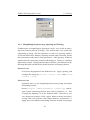
Let’s convert the image to 8-bit. First check the state of "Conversion" option by [Edit > Option > Conversion]. Make sure to tick
"scale when converting".
Do [Image > Type > 8-bit]. The line ROI is still there after the
conversion. Do [Analyze > Plot Profile...]
again. You will
find another graph pops up. Compare the previous profile (16-bit)
and the new profile (8-bit).
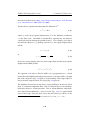
Conversion modifies the y-value. Shapes of the profile look mostly
similar, so if you normalize two images, the curve may overlap. This
is because the image is scaled according to the following formula.
I8 ( x, y) =
I16 ( x, y) − min( I16 ( x, y))
∗ 255
max ( I16 ( x, y)) − min( I16 ( x, y))
where
I16 ( x, y): 16-bit image
min( I16 ( x, y)): the minimum value of 16-bit image
max ( I16 ( x, y)): the maximum value of 16-bit image
I8 ( x, y): 8-bit image
Save the line ROI you created by pressing "t" or clicking on "add" in
the ROI manager (you can open the manager with [Analyze Tools
ROI manager...]). A small dialog window pops up, so click "Add"
button in the right side. The numbers in the left column are names of
the ROIs you add to the manager (they correspond to the coordinates
of the start / end points of the ROI).
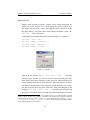
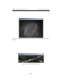
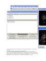
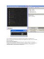
Now, change the option in [Edit > Option > Conversion] by unticking "scale when converting". Open the 16-bit image again by
[File > Open > m51.tif]. Then again, do [Image > Type > 8-bit].
An apparent difference you can observe is that now the picture looks
like a overexposed image. Find the ROI manager window and click
the ROI number you stored in above. Same line ROI will appear in the
new window. Then do [Analyze > Plot Profile...]. This third
profile has a very different shape compared to the previous ones. This
12
EMBL CMCI ImageJ Basic Course
1.1 Basics of Basics
Figure 1.6 – Conversion Option. Scaling is turned off in this case.
is because the values above 255 are now considered as "saturated",
which means that what ever the value is, numbers larger than 255
becomes 255.
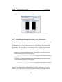
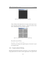
Figure 1.7 – m51 image converted to 8-bit without scaling.
13
EMBL CMCI ImageJ Basic Course
1.1 Basics of Basics
(a)
(b)
Figure 1.8 – (a) Intensity profile of 1.3b. If the conversion was done with scaling, then the
profile would look like (b).
When you perform a conversion, very different results could appear depending on how you scale, like we have just seen. But in many cases, you
do not recognize such changes just by looking at the image: for this reason, one should keep in mind that the conversion may "saturate" or cause
artifacts in the image - screwing up scientific images to non-scientific ones.
1.1.4
Math functions
A digital image is a matrix of numbers. We can calculate images like usual
math. If there is a flat image with pixel value of 10, and if you add 1 to the
image, then all pixel values become 11. We think about a pixel at (5, 10),
and we write down the calculation as follows:
f (5, 10) = 10
(1.1)
g(5, 10) = f (5, 10) + 1 = 11
(1.2)
We generalize this. x and y are the coordinates within the image.
g( x, y) = f ( x, y) + 1
(1.3)
The original image is f ( x, y) and the result after the addition is g( x, y).
Likewise images could also be subtracted, multiplied and divided by number.
14
EMBL CMCI ImageJ Basic Course
1.1 Basics of Basics
Exercise 1.1.4-1
Simple math using 8-bit image: Prepare a new image following the
initial part of the exercise 1.1.1. Now, bring the mouse pointer over
the image and check the "value" that appears in the status bar in the
ImageJ window4 . All pixel values in the image should be"value = 0".
"x=. . . , y=. . . " in the status bar.
Commands for mathematical operations in ImageJ are as follows.
[Process > Math > Add...]
[Process > Math > Subtract...]
[Process > Math > Multiply...]
[Process > Math > Divide...]
Figure 1.9 – Add dialog.
Add 10 to the image: Do [Process > Math > Add...]. A dialog
window pops up and you can for instance input 10 and press OK.
Now, place the mouse pointer over the image to check that the pixel
values actually became 10. Then select the pen tool from the tool bar,
and draw a diagonal line in the window. Check again the pixel value.
The line you just drew has pixel value 255. Then add 10 again to the
image by [Process > Math > Add...]. Check the pixels by placing
the pointer. The black part is now 20, but what happened to the white
4
In the previous exercise 1.1.1, we converted the image to a text file and then checked
the pixel values, but it is also possible to check the value pixel by pixel using this method.
From ImageJ 1.46i (release: Mar. 15, 2012), you could check the pixel values by [Image
> Transform > Image to Results]. This command will send the image matrix
shown in Results window as numbers.
15
EMBL CMCI ImageJ Basic Course
1.1 Basics of Basics
line?
Since the image bit-depth is 8, the available number is only between 0
and 255. When you add 10 to a pixel with its value 255, the calculation
returns 255 because the number "265" does not exist in 8-bit world. A
similar limitation applies to other mathematical operations too. If you
multiply a pixel value 100 by 3, the answer in normal mathematics is
300. But in 8-bit world, that pixel becomes 255.
How about division? Close the currently working test image, and
prepare a new image as you did in 1.1.1. Zoom up the image, and
add 100 ([Process > Math > Add...]; you should see the image
turns to gray from black). Check pixel values by placing the pointer
above the image. Now, Divide the image by 3 ([Process > Math >
Divide...]). Check the result by placing the mouse over the image.
The pixel value is now 33. Since there is no decimal placeholder in 8bit, the division returns the rounded value of (100 / 3 = 33). One could
also divide image by any real number, such as 3.1415. The answer will
be in integer in all cases in 8-bit and 16-bit. In case of floating point
32-bit image, the calculation results are different. We study this in the
next exercise.
Exercise 1.1.4-2
Simple Math on 32-bit Image: prepare a new 32-bit image (in the [New
> Image..] dialog, select 32-bit from the "type" drop-down menu).
Then add 100 to the image. Check that the image pixel values are all
100. Then divide the image by 3. Check the answer. This time the
result has a decimal placeholder.
Bit-depth limitation of digital image is very important for you to know,
in terms of quantitative measurements. Any measurement must be done
knowing the dynamic range of the detection system prior to the measurement. If you are trying to measure the amount of protein, and if some of the pixels
are saturated, then your measurement is invalid.
16
EMBL CMCI ImageJ Basic Course
1.1.5
1.1 Basics of Basics
Image Math
In the previous section we operated on a single image. Likewise, we can
perform computations involving two images. For example, assuming two
images f and g with same dimensions, and
f (5, 10) = 100
(1.4)
g(5, 10) = 50
(1.5)
. . . meaning that the pixel value at the position (5, 10) in the first image f is
100 and in the second image g is 50, we can add these values and get a new
image h such that:
h(5, 10) = f (5, 10) + g(5, 10) = 100 + 50 = 150
(1.6)
This holds true for any pixel at position ( x, y):
h( x, y) = f ( x, y) + g( x, y)
(1.7)
Note that this only works when the image width and height are identical.
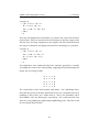
Above is an example of addition. More numerical operations are available
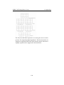
in ImageJ:
Add
img1 = img1+img2
Subtract
img1 = img1-img2
Multiply
img1 = img1*img2
Divide
img1 = img1/img2
AND
img1= img1 AND img2
OR
img1 = img1 OR img2
XOR
img1 = img1 XOR img2
Min
img1 = min(img1,img2)
Max
img1 = max(img1,img2)
17
EMBL CMCI ImageJ Basic Course
1.1 Basics of Basics
Average
img1 = (img1+img2)/2
Difference
img1 = |img1-img2|
Copy
img1 = img2
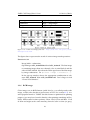
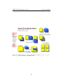
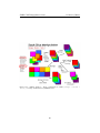
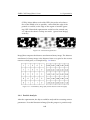
Figure 1.10 – Taken from ImageJ web site. http://rsb.info.nih.gov/ij/docs/
menus/process.html
The figure above represents the result of various image math operations.
Exercise 1.1.5-1
Image Math – subtraction:
Open Images cells_ActinDNA.tif and cells_Actin.tif. The first image
is containing images from two channels. One is actin labeled, and the
other is DNA labeled. We isolate the DNA signal out of the first image
by image subtraction. Do [Process > Image > Calculator...].
In the pop-up window, choose the appropriate combination to subtract cells_Actin.tif from cells_ActinDNA.tif. Don’t forget to tick
"Create New Window".
1.1.6
RGB image
Color images are in RGB format (could also be a so-called pseudo-color
image, or 8-bit color, but this is just because of LUT. See section 1.1.7). Another popular format is "CMKY" but this format is optimized for printing
purpose (you may have heard it already when printing something in Photolab). RGB stands for three primary colors. Red, Green and Blue. If all
of them are bright at the same intensity, then the color is white (or gray).
18
EMBL CMCI ImageJ Basic Course
1.1 Basics of Basics
If only red is bright, then the color is red, and so on. A single RGB image
thus has three different channels. In other words, three layers of different
images are overlaid in a single RGB image. Each channel (layer) has a bit
depth of 8-bit. So a single RGB image is 24-bit image. For this, the file
size of color pics becomes three times larger than a gray scale 8-bit image.
Don’t save 16bit image in RGB format, since you lose a lot of information,
for automatic conversion from 16 to 8 bit takes place.
Exercise 1.1.6-1
Working with RGB image:
(a) Open the image RGB_cell.tif by either [EMBL > Samples] or [File
> Open]. Then split the color image to 3 different images [Image >
Color > Split Channels].
(b) Merge back the images with [Image Color > Merge Channels...].
Figure 1.11 – Color Merge Dialog
In the dialog window, choose an image name for each channel. Uncheck
"Create Composite" and check "keep source images". Then try swapping color assignments to see the effect.
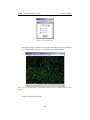
(c) Working on each channel separately: Close all windows and open
the "RGB_cell.tif" again. Do [Image > Color > Channel Tools...].
Then click button "More" and select "Create Composite".
19
EMBL CMCI ImageJ Basic Course
1.1 Basics of Basics
Figure 1.12 – Channel Tool
Resulting image is a three-layer stack and each layer corresponds to
one of R, G or B. Each layer can be processed individually.
Figure 1.13 – Composite image. Note slider at the bottom for switching between three
channels.
Using Channel Tools again,
20
EMBL CMCI ImageJ Basic Course
1.1 Basics of Basics
Figure 1.14 – Channel Tool, now only selected for Channel 2.
Choose "color" from the pull-down tab, instead of "Composite". Select
channel 2 (in this image, this will be Green channel). Select a part of
the image using a rectangular ROI.
Figure 1.15 – ROI selection, in channel 2. Note the position of slider.
Then do [Edit > Clear]. This will pop up a window.
21
EMBL CMCI ImageJ Basic Course
1.1 Basics of Basics
Figure 1.16 – Asking you whether you want to process all channels.
Click No, because you want to process only one channel.
Figure 1.17 – Channel 2 pixel values inside selected ROI becomes 0.
Troubleshooting: If the ROI is not cleared (becomes bright),
then you should change the background color setting. Do
[Edit > Option > Colors...] and you will see a pop-
up window like this.
22
EMBL CMCI ImageJ Basic Course
1.1 Basics of Basics
Figure 1.18 – Color selection dialog.
Make sure that the background is "black". Do the ROI clearing again.
Select "Composite" in the pull-down tab of channel tool.
Figure 1.19 – Choosing Composite, all channels visual.
Resulting image should look like below.
23
EMBL CMCI ImageJ Basic Course
1.1 Basics of Basics
Figure 1.20 – Only channel 2 is devoid of image within the selected ROI.
In this case, the intensity of the green channel in the ROI is now set to
0 ("clear"). You could do such processing of single channel by simply
selecting a channel with the horizontal scroll bar and do the processing directly, such as drawing square ROI and deleting that part in that
channel in "composite" view.
1.1.7
Look-Up Table
We now look at how the matrix of numbers is converted to an image. Let’s
think about a row of pixels with increasing pixel values from 0 to 255 (so
there are 256 pixels in this row). Computer monitor will show a gradient of
intensity that is linearly increasing its brightness from black to white. This
is because the software is giving a command to the monitor, such that "this
pixel ( x, y) is 158 so the corresponding voltage required for this position
( x, y) in the screen should be **mV". For this command to be composed,
software needs a so called "look-up table" (LUT).
The default LUT is the gray scale, that assigns black to white from 0 to 255
in the 8-bit image. In the 16-bit image gray scale will be valued from 0 to
24
EMBL CMCI ImageJ Basic Course
1.1 Basics of Basics
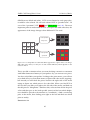
65535 between black and white. LUTs are not limited to such grayscales,
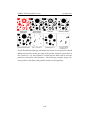
it could be also colored. We call such colored LUT as “pseudo-color”. In
case of the “spectrum” LUT, 0 is red and 100 is green (see 1.21). The most
important point to understand the LUT concept is that with same data, the
appearance of the image changes when different LUT is used.
Look-Up Table
Gray Scale
0
0
0
0
100
0
0
0
0
Look-Up Table
Spectrum
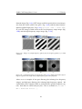
Figure 1.21 – Look-Up Table is a table that defines appearance of pixel values as an image.
With same pixel values, how they are colored could be different, which depends on the
selection of LUT.
This is just like a situation when you start checking a menu in a restaurant
with limited amount of money in your pocket. Say you want to eat a pizza.
You have only €10 in your pocket. Looking at the pizza menu, you will not
try to find what you want from names of pizza and what are the toppings,
but instead you will check the prices listed in the right side of the menu
trying to figure out which pizza is less then €10. When you find €7.5 in
the list, then you slide your sight to the left side of the menu, and find out
that the pizza is "Margherita". Similar to this, software first checks the pixel
value and then goes to the look-up table (menu) to find out which brightness should be passed to the monitor as a command ( = find a convincing
price in the menu, then sliding your sight to the left and find out which
pizza to order).
Exercise 1.1.7-1
25
EMBL CMCI ImageJ Basic Course
1.1 Basics of Basics
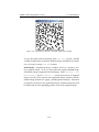
For 8-bit images, there is a default LUT normally called "grayscale".
To see the LUT, open the image Cell_Colony.jpg and then do [Image
> Color > Show LUT]. LUT window pops up showing the relation-
ship between pixel value and pixel intensity. Try to change the LUT
by [Image > Lookup Tables >Spectrum]. Pixel value does not change
by this operation, but the pixel intensity changes that the image appears differently now. Check the LUT again by do [Image > Color
> Show LUT]. Actual numbers in each LUT could be checked using
“’list’ button at the left-bottom corner of each LUT window.
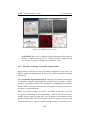
(a)
(b)
Figure 1.22 – Grayscale LUT (a) converted to spectrum LUT (b).
26
EMBL CMCI ImageJ Basic Course
1.1 Basics of Basics
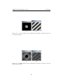
(a)
(b)
Figure 1.23 – (a) Grayscale LUT and (b) spectrum LUT
1.1.8
Image File Formats
In this part I will discuss on issues related to image file formats including:
• Header and Data
• Data Compression
Image file contains two types of information. One is the image data, the
matrix of numerical values. Another is called "header", which contains the
information about the architecture of image. Since software must know
information such as bit-depth, width and height, and the size of the header
before opening the image, the information is written in the "header". The
total file size of an image file is then
Total f ilesize = headersize + datasize
There are many different types of image formats, such as TIFF, BMP, PICT
and so on. The organization of the information in the header is specific to
each format, as is the size of the header. In biology, microscope companies
create their own formats to include more information about the image, such
as the type of microscope used, used objectives, binning, shutter speed,
time intervals, user name and so on.
Having to handle company-specific formats makes our life more difficult
because each image can a priori only be opened from the software provided
27
EMBL CMCI ImageJ Basic Course
1.1 Basics of Basics
by these companies. Fortunately there is an excellent ImageJ plugin which
enables importing specific image formats to ImageJ 5
You do not have to know all the details about the architecture of various
image formats (thanks to the bioformats plugin), but it is important for you
to know that the difference resides mainly in the header. The data part is
in most cases same, something like what we have seen already using text
image (for more details on header, refer to the appendix 1.6.1 ).
Exercise 1.1.8-1
Accessing the image properties
Open the example image wt1.tif. Do [Image > Show Info...]. Scale
(pixels/inch) is listed in the information window, which was read out
from the header of the image. Then do [Image > Properties], also
showing the scale.
Compression: Image file size become huge as the size of the image become
larger. There are convenient ways to reduce image file size by data compression. When you take a snap shot using commercial digital camera or
smart phone, saved images are always compressed. But keep in your mind:
There are two types of compression formats: loss-less and lossy formats. In
loss-less formats, pixel values generated by CCD are preserved even after
the compression is made. On the other hand in lossy formats, pixel values
become different from the original measured values and cannot be restored.
PNG is a popular loss-less compression format that does NOT alter the
original pixel values. With this format, compression of images are done by
shrinking redundant parts: for example, instead of having 100 pixels of 0
values as a block, you could replace that part by saying “here, there are
100 pixels of zeros”. If you need to compress files, using PNG format is
preferred for scientific image data.
Other more popular compression formats are like JPEG and GIF. JPEG is
ofen used in commercial diginal cameras. In addition to the redundancy
shrinking explained above, the compression procedure tries to mathematically interpolate some parts of the image to ignore small details. These
5
LOCI Bioformat Plugin:
http://www.loci.wisc.edu/ome/formats.html
28
EMBL CMCI ImageJ Basic Course
1.1 Basics of Basics
are lossy formats as the process of compression discards some part of data.
This causes artifacts in the image and it could even be "manipulation" of
data. For this reason, we better avoid using lossy formats for measurements as we cannot recover the original uncompressed image once they
are converted.
I recommend not to compress data except for sharing of data for visualization purpose. The PNG format does not lose the original pixel values but
due to the file format conversion, the header information associated with
the original will be lost and this often causes problem in retrieving important information about images such as scales and time stamps.
1.1.9
Multidimensional data
In this section, we study the following topics.
• Image stacks
• Editing Stacks
• 4D stacks
• Hyperstacks
Multidimensional data, in which we define here as a set of image data with
dimensions more than x and y. Multidimensional data have intrinsic limitation in displaying them on two dimensional screen. Efforts have been
made to represent multidimensionality in various ways. One way is the
“image stack”.
stacks
When you take time-lapse sequence or z-sections using a commercial microscope system, the image files are generally saved in the company specific file formats (e.g. .lsm or .lif files). Importing these images into ImageJ
could simply be done using LOCI bioformats plugin.
29
EMBL CMCI ImageJ Basic Course
1.1 Basics of Basics
These image data appear as a series of images contained within a window
with a scroll bar at the bottom. By scrolling, one could go through the
third dimension like a movie. This is the simplest form of multidimensional
representation in 2D display.
In some cases, multidimensional data takes a form of multiple single image
frames with numbering such as
image0001.tif
image0002.tif
image0003.tif. . .
We can import such numbered files recursively and create a stack in ImageJ.
Exercise 1.1.9-1
We import multiple image files as an image stack. Download a zipped
file by [EMBL > Samples > Spindle-Frames.zip] 6 . Unzip the file
by double clicking. Then [File > Import > Image Sequence...]
will open a dialog window and you must specify the first file of the
image series. Select sample sequence eg5_spindle_50000.tif. . . Then
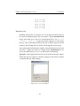
another dialog window pops up (Fig. 1.24).
6 We do also have the stack directly downloadable, but we try to load numberd-tif images
here.
30
EMBL CMCI ImageJ Basic Course
1.1 Basics of Basics
Figure 1.24 – Importing multiple frames as a Stack
ImageJ automatically detects the number of files in the folder, and
then another window opens to ask for the number of images you
want to import, the starting image, the increment between the numbering of the files, and also the common part of the names of the files
you want to import.
For example, if your sequence starts with exp01. . . , then you could
place the text exp01 in the text field of “File name contains”. This then
avoid loading other data set with prefix exp02 even if they are within
the same folder. Regular expression could also be used in the “or
enter pattern” text field7 .
7 If you do not know what Regular Expression is, try the tutorial at http://www.
vogella.com/articles/JavaRegularExpressions/article.html.
For those
who knows what regex is, use the Java regex.
31
EMBL CMCI ImageJ Basic Course
1.1 Basics of Basics
There are other options such as scaling and conversion of the image
bit depth, but these operations could be done afterward. The imported image sequence is within one window, or a stack.
A stack could be saved as a single file. File extension is typically ".tif",
which is same as the single frame file. The file header will contain the
information on the number of frames that the image contains. This
number will be automatically detected when the stack is opened next
time, so that the stack can be correctly reproduced.
Don’t close the stack, exercise continues.
Exercise 1.1.9-2
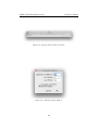
In the ImageJ tool bar among all the tool icons, there is a button with
“Stk”. All the commands related to stack can be found there by clicking that icon.
Figure 1.25 – ImageJ tool bar in default mode.
[Start Animation] plays the sequence as animation. This com-
mand can be found at [Image > Stacks > Tools > Start Animation].
Try changing the playback speed by [Animation Options]. This
command pops up a dialog to set the playback speed. In the main
menu, this same command is at [Image > Stack > Tools > Animation
options...]
To exclusively work on stacks, there is an icon » at the right most
position in the ImageJ menu bar. Click and then from drop down
menu that appeared, select "Stack tools". Video player-like interface
appears in the tool bar (1.26). Try different buttons to see what action
32
EMBL CMCI ImageJ Basic Course
1.1 Basics of Basics
Figure 1.26 – ImageJ tool bar in Stack Tool mode.
Figure 1.27 – Animation Option Window
33
EMBL CMCI ImageJ Basic Course
1.1 Basics of Basics
they perform.
Editing Stacks
In many occasions you might need to edit stacks such as
• Truncate a stack because you only need to analyze a part of the sequence.
• For a presentation you need to combine two different stacks.
• Need to add a stack at the end of another stack.
• To make a combined stack by attaching each frame in a stack by a
frame of another stack. Typically, you want to have two channels of
image side-by side,
• You need only every second frame or slices to reduce the stack size
by a half.
• To split two channel time series to individual time points without
splitting the channels.
• You need to insert a small inset within a stack.
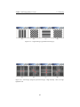
For such demands, tools for stack editing are available under the menu
tree [Image > Stack > Tools]. Figure 1.28 and figure 1.30 schematically
shows what each of these commands does.
Exercise 1.1.9-3
Creating a Montage
Create a new image [File > New > Image...] with the following
properties.
Name: could be any thing
• Type: 8-bit
• Fill with: Black
• Width: 200
34
EMBL CMCI ImageJ Basic Course
Figure 1.28 – Editing Stacks 1.
1.1 Basics of Basics
These commands are under [Image > Stack >
Tools]. Courtesy of Sebastién Tosi, IRB Barcelona.
35
EMBL CMCI ImageJ Basic Course
Figure 1.29 – Editing Stacks 2.
1.1 Basics of Basics
These commands are under [Image > Stack >
Tools]. Courtesy of Sebastién Tosi, IRB Barcelona.
36
EMBL CMCI ImageJ Basic Course
1.1 Basics of Basics
• Height: 200
• Slices: 10
Then draw time stamps in each frame by Image > Stacks > Time
Stamper with the default properties but for the following:
X location: 50
• Y location: 90
• Font Size: 36
Now, you should have printed time for each frame, 0 to 9 sec. To
make a montage of this image stack, do [Image > Stacks > make
Montage...]. Set the following parameters and then click OK.
Columns: 5
• Rows: 2
• Border Width: 1
• Label Slices: checked.
Figure 1.30 – Montage of the time-stamped stack.
If you have time, try to change the column and row numbers to create
montage with different configuration.
Concatenation
Then duplicate the time stamp stack, concatenate the duplicate to the
original ([Image > Stacks > Tools > Concatenate...]). Create
a montage of this double sized stack.
37
EMBL CMCI ImageJ Basic Course
1.1 Basics of Basics
4D stacks
A time-lapse sequences (we could call it “2DT stack” or xyt stack) or a Zstack (we could call it “3D stack” or xyz stack) are relatively simple objects
because they are both made up of a series of two dimensional images. More
highly dimensioned data are common these days. In many occasions we
take a time series of z-stacks maybe also with multiple channels. The order of two dimensional images within such multidimensional stacks then
becomes an important issue. If we take an example of 3D time series, a possible order of 2D images could start first with z-slices and then time series.
In this case, the frame sequence will be something like this:
imgZ0-T1.tif
imgZ1-T1.tif
imgZ2-T1.tif
imgZ0-T2.tif
imgZ1-T2.tif
imgZ2-T2.tif
imgZ0-T3.tif
...
The number after “Z” is the slice number and that after “T” is the file name.
We often call this order “XYZT”. Alternatively, 2D images could be ordered
with time points first and then z-slices. In this case images will be stacked
as:
imgZ0-T1.tif
imgZ0-T2.tif
...
imgZ1-T1.tif
imgZ1-T2.tif
...
imgZ2-T1.tif
imgZ2-T2.tif
...
We call this order “XYTZ”.
The order you will often find is the first one (XYZT) but in some cases you
38
EMBL CMCI ImageJ Basic Course
1.1 Basics of Basics
might also find the second one (XYTZ).
Stacks with more than 4D
If we have multiple channels, we could even have an order like “XYCZT”8
and so on. Since when viewed as a regular stack we can scroll only along a
single dimension the order of stack dimensions is fundamental as it effects
the order in which the images will appear.
To avoid such complication with dimension ordering, there is an advanced
format of stack called Hyperstack. It could have up to three scroll bars at the
bottom for channels (C), slices (Z) and time points (T) so one could easily
scroll through the dimension of your choice 1.31.
We will study more on the actual use of the image stacks in section 1.5.
Exercise 1.1.9-2
In this exercise, you will learn how to interact with image stacks (n Dimensional images). Open sample image stack yeastDivision3DT.tif.
This is a 3D time series stack. You can browse through the frames by
moving the scroll bar at the bottom of the frame. Since this is a 3D
time series, you will see that each time point is a sub-stack of images
at different optical sections.
To view the stack in a more convenient way, you could convert the
stack to a hyperstack by
[Image > Hyperstacks > Stack to Hyperstack...].9
In “Hyperstack” mode, two scroll bars appear at the bottom of the
window. One is for scrolling through z slices and the other to select a
time point (frame). Each scroll bar could be moved independently of
the other dimension, so you could for example go through the time
8 XYCZT
is a typical order but many microscope companies and software do not follow
this typical order.
9 If this conversion does not work properly, the first thing you could check is if the setting
of the image dimension is properly set. To check this, [Image > Properties...]
and check if slice (z) number and frame number (time points) are set correctly. For the
sample image we use in this exercise, z should be 8 and frames should be 46.
39
EMBL CMCI ImageJ Basic Course
1.1 Basics of Basics
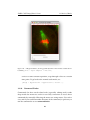
Figure 1.31 – A Hyperstack data, showing spindle dynamics. This 5D data could be downloaded by [File > Open Samples > Mitosis]
series at a same constant z-position, or go through z-slices at a certain
time point. To go back to the normal stack mode, use
[Image > Hyperstacks > Hyperstack to Stack...].
1.1.10
Command Finder
Commands for these stack related tools (especially editing tools) reside
deep inside the menu tree and it is not really convenient to access those
commands by manually following the menu tree using mouse. For such a
case, and if you could remember the name of the command, a quick way to
run the command is to use command finder.
40
EMBL CMCI ImageJ Basic Course
1.1 Basics of Basics
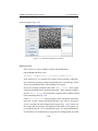
There is a short cut key to start up the command finder: control-l in windows and in mac OSX command-l. On start up, the command finder interface looks like figure 1.32a. Type in the command that you want to use in
the text field labeled “search”, and then menu item is filters as you type in
(fig. 1.32b). Select the one you want and then click the button “run”. This
is the same as selecting that command from the menu tree. This tool is also
useful when you know the name of a command but forgot where it is in the
menu tree, since it also shows where the command is by showing its menu
path.
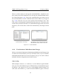
(a) The interface on start up.
(b) Typing in some command name will
filter the menu items and shows the hits.
Figure 1.32 – Command Finder.
1.1.11
Visualization of Multidimensional Images
We have an intrinsic limitation in displaying multidimensional images, but
we still want to check data by our eyes. For this reason, ways to visualize
multi-dimensional data have been developed. We go over some of those
methods which are frequently used in this section.
Color Coding
With multiple channels, we could have several different signal distributions per scene from different types of illuminations or from different types
of proteins. One typical way to view such multiple channel image is to
color code each channel e.g. actin in red and Tubulin in green. We have
41
EMBL CMCI ImageJ Basic Course
1.1 Basics of Basics
already scene such images in the RGB section (1.1.6).
The color coding is not limited to the dimensions in Channels, but also for
slices (Z) and time points (T). By assigning a color that depends on the slice
number or time points, the depth information within a Z-stack or a time
point information with in a time lapse movie could be represented as a
specific color rather than by the position of that slice or frame within image
stack.
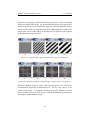
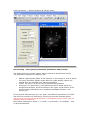
Exercise 1.1.11-1
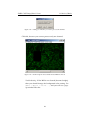
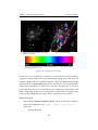
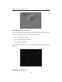
Open [EMBL > Samples > TransportOfEndosomalVirus.tif ]. Apply the color coding to this time-lapse movie [Image > HyperStacks
> Temporal-Color Code]. In the dialog choose a color coding ta-
ble from the drop-down list. Principle of the coding is same as the
look-up table, and only the difference is that the color assignment is
adjusted so that the color range of that table fits to the range of frames
(fig. 1.33).
Projection
Projection is a way of decreasing an n-dimensional image to an n-1-dimensional
image. For example, if we have a three dimensional XYZ stack, we could
do a projection along Z-axis to squash the depth information and represent
the data in 2D XY image. We lose the depth information but it helps us to
see how the data looks like. The principle is like this: we could think of
XYZ data as a cubic entity. This cube is gridded and composed of small
cubic elements. If we have a Z-stack with 512 pixels in both XY and with 10
slices in Z, we then have a cube composed of 512 x 512 x 10 = 2,621,440 small
cubes. These small cubes are called “voxels”, instead of “pixels”. Now, if
we take a single XY position, there are 10 voxels at this XY position (figure
1.34).
Imagine the column of 10 voxels: Each voxel has a given intensity, and we
can compute statistics over these 10 values such as the mean, the minimum,
the maximum, the standard deviation and so on. We can then represent this
column by a single statistical value.
42
EMBL CMCI ImageJ Basic Course
1.1 Basics of Basics
(a) Original stack, first frame. This stack
consists of 72 frames.
(b) Color coded stack.
(c) Scale of the time color-coding. From frame 1 to 72, corresponding
color is shown as a scale.
Figure 1.33 – Temporal-Color Coding.
In this way, we can pick up a column of voxels from every XY positions,
compute statistics and create a two dimensional image with each of its XY
position filled with voxel column statistics. This two dimensional image
is the result of the projection along Z-axis, or what we call “Z-projection”.
Projection could also be in other axes, not only along Z-axis. If we do a
projection along X-axis, we would then have a projection of the data to YZ
plane. Projecting aloing Y-axis will result in a projection to XZ plane (this
relates to the orthogonal viewing, which we try in the next section).
Exercise 1.1.11-2
Open image mitosis_anaphase_3D.tif. Then do all types of projections you could choose by [Image > Stack > Z projection...].
There are
Average Intesnity
43
EMBL CMCI ImageJ Basic Course
1.1 Basics of Basics
z
y
x
Figure 1.34 – A three dimensional stack can be regarded as a gridded cube. The projection calculates various sorts of statistics for each two dimensional positions , which can be
viewed as a stack of voxels, and store that value in the two dimensional image at the same
position.
• Max Intensity
• Min Intensity
• Sum of Slices
• Standard Deviation
• Median
Question 1: Which is the best method for knowing the shape of the
chromosome?
Question 2: Discuss the difference of projection types and why there
is such difference.
“Max Intensity” projection is the most frequently used projection method
in fluorescence microscopy images, as this method picks up bright signals.
44
EMBL CMCI ImageJ Basic Course
1.1 Basics of Basics
“sum of slices” method returns a 32bit image since results of addition could
possibly exceed 8 bit or 16 bit range.
Note 1: If your data is a 3D time series hyper stack, there will be a small
check box in the projection dialog "All Time Points". If you check the box,
projection will be done for each time point and the result will be a 2D time
series of projections.
Note 2: The projection of a 2D time series can also be performed. Thought
the command name is “Z-Projection”, the principle of projection is identical
regardless of the projection axis.
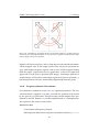
Orthogonal Views
The projection is a convenient method for visualizing 3D stack on 2D plane,
but if you want to preserve the original dimensions and still want to visualize data, one way is to use a classic 2D animation. This could be achieved
easily with the scroll bar at the bottom of the each stack. But this has limitation: we could only move in the third dimension, Z or T. To scroll through
X or Y, we use “Orthognlal View”.
You could view a stack in this mode by [Image > Stack > Orthogonal
View]. Running this command will open two new windows at the right
side and below the stack. These two new windows are showing YZ plane
and XZ plane. Displayed position is indicated by yellow crosses. These
yellow lines are movable by mouse dragging.
Exercise 1.1.11-3
Open image mitosis_anaphase_3D.tif. Run a command [Image >
Stack > Orthogonal View]. Try scrolling through each axes: x, y
and z.
3D viewer
Instead of struggling to visualize 3D in 2D planes, we could also use the
power of 3D graphics to visualize three dimensional image data. 3D viewer
45
EMBL CMCI ImageJ Basic Course
1.1 Basics of Basics
(a) XY
(b) YZ
(c) XZ
Figure 1.35 – Orthogonal View of a 3D stack.
is a plugin written by Benne Schimidt. It uses Java OpenGL (JOGL) to render three dimensional data as click-and-rotatable object on your desktop.
We could try to use the 3D viewer with the data we have been previously
dealing with.
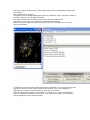
Exercise 1.1.11-4
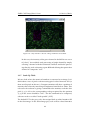
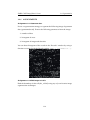
Open image mitosis_anaphase_3D.tif. Run a command [Plugins
> 3D Viewer]. A parameter input dialog opens on top of 3Dviewer
window. Change the following parameters:
Image: Choose mitosis_anaphase_3D.tif.
• Display as: Choose Surface.
• Color: Could be any color. In the example shown in fig.1.36,
white was chosen.
• Threshold: Default value 50 should work OK, but you could also
try changing it to greater or smaller values. This threshold value
determines the surface. Pixel intensity greater than this value
will be considered as object, else background.
• Resampling factor: default value (2) should be sufficient. If you
change this value to 1, then it takes longer time for rendering.
46
EMBL CMCI ImageJ Basic Course
1.1 Basics of Basics
In case of our example image which is small, difference in the
rendering time should be not really recognizable.
After setting these values, clicking “OK” will render the image in the
3Dviewer window. Try to click and rotate the object.
(a) Parameter Input Dialog
(b) Surface rendered 3D stack
Figure 1.36 – Surface rendering by 3DViewer.
More advanced usages are available such as visualizing two channels or
showing 3D time series as a time series of 3D graphics or saving movies.
For such usages, consult the tutorial in the 3DViewer website (http://
3dviewer.neurofly.de/).
1.1.12
Resampling images (Shrinking and Enlarging)
When you want to check the details of images, zooming is the best way
to focus on a specific region to observe details. Zooming is done by the
magnification tool (icon of magnification glass) and this simply enlarges or
shrinks the pixels.
Instead if you really need to increase the number of pixels per distance, we
call such processing as “Resampling” and we will examine this a bit in this
section.
By the way, if we just want to have larger image by adding some margin,
47
EMBL CMCI ImageJ Basic Course
1.1 Basics of Basics
we call this “resizing”, and the command for this resides in the menu tree
under [Image > Adjust > Canvas Size].
The resampling changes the original data. If we have an image of size 10
pixels by 10 pixels and resample it to 200%, the image becomes 20 x 20. If
we resample it by 50%, then the image becomes 5 x 5. The resampling is
a simple task that could be done by [Image > Adjust > Size...]. This
is a simple operation but one must take care about how pixels will be produced while enlarging and reduced while shrinking. If the enlarging is
simply two times larger, we could imagine that each pixel will be copied
three times to produce a block of four pixels to complete the task. The pixel
values of the newly inserted pixels will then be identical to the source pixel.
But what happens if we want to enlarge the image by 150 %? To simplify
the situation, think about an image with 2 x 2 pixels. Then the resulting
image becomes 3 x 3. To understand the effect, do the following exercise.
Exercise 1.1.12-1
Open the example image 4pixelimage_sample.tif. The image is ultra
small, so zoom it up to the maximum (as much as you can, you must
click on or Ctrl - +). You now see four pixels in the window. Duplicate the image by [Image > Duplicate]. Magnify again. "Select all"
by [Edit > Selection > Select All]. Then [Image > Adjust
> Size...]. In the dialog window, input the width 4 and height 4
(corresponds to 200% enlargement). Tick "aspect ratio" and un-tick
"Interpolation". Then click OK. Check the pixel values in original image, and the enlarged image.
Exercise 1.1.12-2
Do the similar resampling, but this time enlarge the image by 150%.
Check the pixel values.
The resampling in the exercise was without interpolation – the check box
was OFF. Interpolation is similar to the one dimensional interpolation we
do with graphs. In case of images, the gradient is also two dimensional
so the situation is a bit more complex. There are various methods for interpolating image. The interpolation method used in ImageJ is the bilinear
48
EMBL CMCI ImageJ Basic Course
1.1 Basics of Basics
(a)
(b)
Figure 1.37 – Artifacts produced by resizing. (a) Four pixel image and (b) nine pixel image
after resizing.
interpolation. Briefly, the bilinear interpolation algorithm samples pixel values in the surrounding of the insertion point, and calculates the pixel value
for that position10 . One must keep in mind that the result of enlarging or
shrinking of image depends on the interpolation method – and scientific results could be altered depending on the method you use. In a more general
context, this problem is treated as “sampling theory”. With this keyword,
search more explanation in information theory textbooks and in the Internet.
10 For more details on bilinear interpolation, refer to
http://www.cambridgeincolour.com/tutorials/image-interpolation.htm.
49
EMBL CMCI ImageJ Basic Course
1.1.13
1.1 Basics of Basics
ASSIGNMENTS
Assignment 1-1-1: Digital image = matrix of numbers
Edit a text image using any text editor. Be sure to insert space between
numbers as separator. Save the text file and open it as an image in ImageJ
by importing text image function.
Assignments 1-1-2: bit depth
1. How many gray scale steps does a 12-bit image have?
2. Describe in text how a 1-bit image looks like.
Assignment 1-1-3: bit depth conversion
Use m51.tif (16-bit!) sample image to draw a plot profile, as we did in
the course. In the profile plot window, a "list" button is at the left-bottom
corner. Click the button. You will then see a new window containing a
column of numbers. These numbers can be copy & pasted to spread sheet
software such as LibreOffice or MS Excel( or import the buffer to R). You
could then plot the profile in those applications.
Compare original 16bit profile, 8-bit profiles with and without scaling by
plotting three curves in a graph, and discuss the difference.
Assignments 1-1-4: Simple math on Images
1. Try subtracting certain values from the image you created in the Assignment 1-1-1 and check that the values cannot be less than 0.
2. Prepare an 8-bit image with pixel value 200. Divide the image by 3,
and check the result.
3. Prepare a 16-bit image. In the [File > New > Image...] dialog,
select 16-bit from the "type" drop-down menu. Try adding certain
value to check the maximum pixel value.
4. Discuss why measurement of fluorescence intensity using digital image is invalid when some pixels are saturated.
50
EMBL CMCI ImageJ Basic Course
1.1 Basics of Basics
Assignments 1-1-5: LUT
Open "Cell_Colony.tif". Use LUT edit function and design your own LUT
to highlight the black dots in Green and the background in Black. "LUT editor" can be activated by [Images > Color > Edit LUT...]. Instruction
for the LUT editor is at
http://rsb.info.nih.gov/ij/plugins/lut-editor.html
You might be able to manage using it without reading the web instruction;
just try!). LUT (.lut file) could also be edited using Excel.
Assignments 1-1-6: File size and image bit depth, image size
If there is an image with width = 100 pixels and height = 200 pixels, what
would be the expected size of the image file in bytes? 1 byte = 8-bit.
Create a new image with the dimension as above, and save the image in
"bitmap (.bmp)" format and check the file size. Is it same as you expected,
or different? Save the same image in text file format and check the file size
again.
Assignment 1-1-7 Resizing
1. Enlarge the sample image 4pixelimage_sample.tif by 150% while the
"Interpolation" check box in the size adjustment window is ON. Study
the pixel values before and after the enlargement. What happened?
Describe the result.
2. Change "canvas size" by [Image > Adjust > Canvas Size] for any
image. What"s the difference to "Resize"?
51
EMBL CMCI ImageJ Basic Course
1.2
1.2 Intensity
Intensity
An image has only one type of information: a distribution of intensity. The
image analysis in biology deals with this distribution in quantitative ways.
We investigate the distribution from different angles using various algorithms and analyze biological phenomena such as shapes, cell movements
and protein-protein interactions. For example in GFP labeled cells, intensity of signal is directly related to the density of the labeled biological component. We now start studying how to interpret signals, and how to extract
biologically meaningful numerical values out of intensity distribution.
1.2.1
Histogram
If there is an 8-bit image with 100 pixel width and 100pixel height, there
are 10,000 pixels. Each of these pixels has certain pixel value. Intensity histogram of an image is a plot that shows distribution of pixel counts over a
range of pixel values, typically its bit depth or between the minimum and
the maximum pixel value with in the image. Histogram is useful for examining the signal and background pixel values for determining a threshold
value to do segmentation. We will study image threshold in 1.4).
Exercise 1.2.1-1
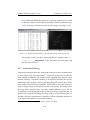
Open Cell-Colony.tif. Do [Analyze > Histogram]. A new window
appears. The x-axis of the graph is pixel value. Since the image bitdepth is 8-bit, the pixel values ranges from 0 to 255. The y-axis is the
number of pixels (so the unit is [count]). Since 255 = white and 0 =
black, the histogram has long tail towards the lower pixel value. This
reflects the fact that the image has white background and black dots.
Check pixel values in the histogram by placing the mouse pointer
over the plot and move it along the x axis. Pixel count appears at the
bottom of the histogram window. Switch to the cell colony image,
and place the pointer over dark spot. Read the pixel value there, and
then try finding out the number of pixels with the same value in the
histogram. What is the range of pixel values which corresponds to
the spot signal?
52
EMBL CMCI ImageJ Basic Course
1.2 Intensity
Histogram could also be used for enhancing contrast of image. Several
different algorithms are available for this: histogram normalization, histogram equalization and local histogram normalization.
If the histogram is occupying only part of the available dynamic range of
image bit depth (8-bit: 0 – 255, 16-bit: 0 – 65535), we could adjust pixel values of image to increase its range so that contrast become more enhanced.
There are two ways to do this: normalization and equalization.
Normalization
With normalization, pixel values are normalized according to the minimum
and the maximum pixel values in the image and bit-depth. If the minimum
pixel value is pmin and the maximum is pmax in an 8-bit image, then normalization is done as follows:
NewPixelValue =
(OriginalPixelValue − pmin)
∗ 255
(pmax − pmin)
Equalization
Equalization converts pixel values so that the values are distributed evenly
within the dynamic range. Instead of describing this in detail using math
formula, I will explain it with a simple example (see Fig. 1.38). We consider an image with its pixel value ranging between 0 and 9. We plot the
histogram from this image, the result looks like in the figure 1.38a. For
equalization, a cumulative plot is first prepared from such histogram. This
cumulative plot is computed by progressively integrating the histogram
values (see Fig. 1.38b, black curve). To equalize (flatten) the pixel intensity
distribution within the range 0-9, we would ideally require a straight diagonal cumulative plot (in other words, the probability density of the pixel
intensity distribution should be near-flat). To get such plot, we need to
compensate the histogram by shifting values from the bars 5 and 7 to the
bars 7 and 9, respectively (now, bars are in red after shifting). After this
shifting the cumulative plot now looks more straight and diagonal (Fig.
1.38b right, red curve).
53
EMBL CMCI ImageJ Basic Course
1.2 Intensity
(a)
(b)
Figure 1.38 – (a) Histogram Equalization: Very simple case. The actual calculation uses
cumulative plots (b) of the histogram of original image, and uses it as a look up table to
convert original pixel value, applied point-by-point.
Exercise 1.2.1-2
Histogram Normalization and Equalization:
Open sample image g1.tif, and then duplicate the image by [Image
> Duplicate]. Click the duplicate and then [Image > Process >
Enhance Contrast]. A dialog window pops up. Set "Saturated Pix-
els" to 0.0% and check "Normalize", while unchecking "Equalize Histogram", then click OK. Compare histogram of original and normalized images .
Duplicate g1.tif again by [Image > Duplicate]. Click the duplicate
and then [Image > Process > Enhance Contrast]. A dialog window pops up. Set "Saturated Pixels" to 0.0% and uncheck "Normalize", while check "Equalize Histogram", then click OK. Compare histogram of original, normalized and equalized images ([Analyze >
Histogram]).
Exercise 1.2.1-3
Local Histogram Equalization (Optional):
Histogram equalization could also be performed on a local basis. This
becomes powerful, as more local details could be contrast enhanced.
You could try this with the same image g1.tif, by [Pligins > CMCICourseModules
54
EMBL CMCI ImageJ Basic Course
1.2 Intensity
> CLAHE] (if you have installed the course plugin in ImageJ) or if you
are using Fiji, [Process > Enhance Local Contrast (CLAHE)]
1.2.2
Region of Interest (ROI)
To apply certain operation to a specific part of the image, you can select a region by "region of interest (ROI)" tools. The shape of the ROI could be various, such as rectangular, elliptical, polygon, free hand or a line (straight,
segmented or free hand). There are several functions that will be used often
in association with ROI tools.
Exercise 1.2.2-1
Cropping. Open any image. Select a region by rectangular ROI. Then
[image > Crop]. This will remove the unnecessary part of the im-
age, to reduce calculation time.
Exercise 1.2.2-2
Masking. Open any image. Select a region by rectangular ROI. Then
[Edit > clear]. [Edit > Clear Outside]. After checking what
happened, do [Edit Fill]. (same operation could be done by [Edit
> Selection > Crate Mask])
Exercise 1.2.2-3
Invert ROI. Open any image. Select a region by rectangular ROI. Then
[Edit > Selection > Make Inverse]. In this way, you can select
region excluding the region you initially selected.
Exercise 1.2.2-4
Redirecting ROI. Open any two images. In one of the image, select a
region by rectangular ROI. Then activate the other image by clicking
that window, and do [Edit > Selection > Restore Selection].
ROI with same size and position will be reproduced in the window.
Exercise 1.2.2-5
ROI manager. You can store the position and size of the ROI in the
memory. Select a region by rectangular ROI. Then [Analysis >
55
EMBL CMCI ImageJ Basic Course
1.2 Intensity
Tools > Roi Manager]. Click "Add" button to store ROI informa-
tion. Stored ROI can be saved as a file, and could be loaded again
when you restart the ImageJ.
1.2.3
Intensity Measurement
As you move the mouse pointer over individual pixels, their intensity value
are indicated in the ImageJ menu bar. This is the easiest way to read pixel
intensities, but you can only get the values one by one. Here we learn a
way to get statistical information of a group of pixels within ROI. This has
more practical usages for research.
To measure pixel values of a ROI, ImageJ has a function [Analyze > Measure].
Before using this function, you could specify the parameters you want to
measure by [Analyze > Set measurements]. There are many parameters in the "Set measurement" window. Details on these parameters are
listed in the Appendix 1.6.4. For intensity measurements following parameters are important.
• Mean Gray Value - Average gray value within the selection. This is
the sum of the gray values of all the pixels in the selection divided by
the number of pixels. Reported in calibrated units (e.g., optical density) if Analyze/Calibrate was used to calibrate the image. For RGB
images, the mean is calculated by converting each pixel to grayscale
using the formula gray = 0.299red + 0.587green + 0.114blue or the formula gray = (red + green + blue)/3 if "Unweighted RGB to Grayscale
Conversion" is checked in Edit/Options/Conversions.
• Standard Deviation- Standard deviation of the gray values.
• Min & Max Gray Level - Minimum and maximum gray values within
the selection.
• Integrated Density - The sum of the values of the pixels in the image
or selection. This is equivalent to the product of Area and Mean Gray
Value. The Dot Blot Analysis example demonstrates how to use this
measurement to analyze a dot blot assay.
56
EMBL CMCI ImageJ Basic Course
1.2 Intensity
A short note on image-based fluorometry: In biochemical experiments, scientists measure protein concentration by measuring absorbance of UV light
or by labeling proteins with dyes or fluorescence and measure the intensity
of emission. This is because light absorbance or the intensity of fluorescence intensity is proportional to the density of protein in the irradiated
volume within cuvette. Very similar to this when fluorescence image of
cells are taken, pixel values (which is the fluorescence intensity) are proportional to the density of the labeled protein at each pixel positions. For
this reason, measurement of fluorescence intensity using digital imaging
could be considered as the two dimensional version of the conventional
fluorometry.
Exercise 1.2.3-1
Open a sample image cells_Actin.tif. Before actually executing the
measurement, do [Analyze > Set Measurements]. A dialog window opens. There are many parameters listed in the upper-half of the
window.
The parameters we select now are:
• Area
• Integrated Density
• Mean Gray Value
Check the box of these three parameters. Integrated density is the
sum of all the pixel values and Mean Gray Value is the average of all
the pixel values within ROI. So
IntegratedDensity = Area ∗ MeanGrayValue
Select one of the cells in cell_Actin.tif image and zoom it up using
magnifying tool. Switch the tool to "Polygon" tool. Draw polygon
ROI around the cell. Then do [Analyze > Measure]. A window
titled "Results" pops-up, listing the measured values. Check that the
integrated density is the multiplication of area and the mean gray
value.
This value is not the actual intensity of the fluorescence within the cell
since it also includes the background intensity (offset). Measure the
57
EMBL CMCI ImageJ Basic Course
1.2 Intensity
Figure 1.39 – Set Measurement Window
(a)
(b)
Figure 1.40 – (a) Tracing Cell Edge by Segmented ROI and Measuring the Intensity within
selected area.
58
EMBL CMCI ImageJ Basic Course
1.2 Intensity
background intensity by creating a new ROI in the area where there
is no cell.
Figure 1.41 – Measurement of Background
NOTE: When no ROI is active (no yellow bounding rectangle or so), then
the measurement is performed on the whole image.
1.2.4
Image transformation: Enhancing Contrast
Some of you might already have experience with the contrast enhancing of
digital images, since in most of imaging software like the ones that come
with digital camera usually have this function. Low contrast images have
small difference in the tones and the objects are difficult to observe. If the
contrast is too high, then the tone difference is so much that the picture is
"over exposed". Adjustment of contrast controls the tone difference to optimize the visual resolution. The contrast enhancement primarily changes
the LUT, so that the original image data is unaffected (you will see in the
following exercise). The original data is changed only when you click "Apply" button. Then the pixel values are re-scaled according to the LUT you
set.
Care must be taken for contrast enhancement since pixel values are altered.
This could be regarded as "fraud" or "manipulation" in science, especially
if you are measuring image intensity. If all images that you are trying to
compare were equally contrast enhanced, then the images could eventually
be compared. Even then, there will be another pit-fall if you artificially
59
EMBL CMCI ImageJ Basic Course
1.2 Intensity
saturate the image: this happens often especially in the case of low bitdepth images.
Exercise 1.2.4-1
Open image gel_inv.tif. Do [Image > Adjust > Brightness/Contrast].
Pop-up window appears which looks like the figure below (left). The
graph shown in the upper part of the window is the histogram of the
image just like you have seen in section 1.2.1 Histogram. Since the image is 8-bit, scale in the x axis is 0 to 255. There is also a black diagonal
line. This corresponds to the LUT of the image on the screen: pixel
values in x is translated into the gray value on the screen (brightness
on the screen is y-axis).
The slope and position of the LUT can be altered by click and dragging four sliding bars under the graph, each with the name minimum,
maximum, brightness and contrast. Try changing these values and
studying the effect on the image.
QUESTION: What is the problem with the adjustment shown in the
right side of the figure below?
(a)
(b)
Figure 1.42 – (a) Histogram of gel_inv.tif before enhancing contrast. (b) Some bad adjustments example.
Exercise 1.2.4-2
Continued from above: the original image file is not changed at this
60
EMBL CMCI ImageJ Basic Course
1.2 Intensity
stage. When you push "Apply" button at the bottom-right corner, the
original image is altered numerically. Try set the LUT as you like,
and push the Apply: what happened to the Histogram and the LUT
indicator? (you can always "Undo" the "Apply" by [Edit > Undo],
or revert to the original file by [File > Revert]).
Exercise 1.2.4-3
With RGB image, it is possible to adjust the brightness and contrast
for individual color channel. Open the image RGB_cell.tif, then do
[Image > Adjust > Color Balance]. There is a pull-down menu
to specify the channel you want to change. Try changing different
channels to optimize the image.
1.2.5
Image correlation between two images: co-localization plot
In many experiments we need to compare the localization of two or more
proteins and examine whether those proteins are co-localized. In many
cases this has been evaluated by visual inspections. But with digital images, it is possible to evaluate the degree of co-localization more quantitatively. This is done by plotting a so called "co-localization plot". To do
this in ImageJ one could download a plugin Colocalization_Finder11 and
install it.
The level of colocalization could be then parametrized by using statistical
values such as Pearson’s coefficient and Mander’s coefficient. These values have advantages and disadvantages depending on the image properties. For detailed description on these issues, refer to Bolte and Cordelières
(2006).
Additional insights, pitfalls and tips on localizing spot signals could be
found in Waters (2009). This paper also provides detailed examination of
the precision of dot detections.
11 download
from
colocalization-finder.html
http://rsb.info.nih.gov/ij/plugins/
61
EMBL CMCI ImageJ Basic Course
1.2.6
1.2 Intensity
ASSIGNMENTS
Assignment 1-2-1:
Suppose that you have an 8-bit grayscale image showing three objects of
distinct intensities against a bright background. What would the corresponding histogram look like?
Assignment 1-2-2:
With image cell_Actin.tif, do the measurement with 4 cells and one background in image as we did in the exercise. This time, store ROI in ROI
manager (refer to 1.2.2 Roi) and do the measurement at once. First, you
store 5 different ROI one by one ("Add" button). Then click "Show all" button in the ROI manager. Activate all ROI by clicking the ROI name in the
list while pushing down the SHIFT key. Then click "Measure" button. All
five ROI will be measured at once. Average the values and describe the
results in text.
Assignment 1-2-3:
1. Optimize the contrast of image m51_8bit.tif. Be careful not to saturate the pixels so you don’t throw away important information in the
lower pixel values. Check the histogram. Don’t close the histogram
window
2. After applying the adjustment above (clicking "Apply" button), check
the histogram again. Compare the histogram before and after. What
happened? Discuss the reason.
62
EMBL CMCI ImageJ Basic Course
1.3
1.3 Filtering
Filtering
Filtering can improve the appearance of digital images. It can help identifying shapes by reducing the noise and enhancing the structural edge. Not
only for the appearance, filtering improve the efficiency of "segmentation"
which we will study in the next section. Segmented image could be used as
a mask to specify regions to be measured. Note that the filtering alters the
image so one must realize that in most cases, processed images cannot be
used for quantitative intensity measurement without precise knowledge of
how the processing affects the numerical values.
There are two different types of filtering: one involves the frequency domain of images (Fourier transformed image), while the others deals with
spatial domain. We first study the spatial filtering and its central concept
"convolution", and walk through various types of convolutions. We then
study the frequency domain filtering (FFT). In the FFT world, convolution
of an image with filter kernel could be done simply by multiplication between two images.
1.3.1
Convolution
In the [Process] menu, we see a long list of filters. Most of them are
linear filters and can be implemented as "convolution" as we will shortly
see. To perform a convolution a small mask (called kernel) is moved over
the image pixel by pixel and apply operations involving the surrounding
pixel values (see Fig. 1.43). The result of operation is written to that pixel
position in the output image.
To understand how the convolution is done, we take a one-dimensional
example (Fig. 1.44).
We have a small 1D array f , and we want to convolve a kernel w (i). We
first rotate the kernel by 180 degrees that the order is now reversed. Then
we align f and w to match the position of the last element of kernel to the
first element of f . Since we want to have all the kernel elements to have
corresponding partner, we "pad" f by 0. This is just for the convenience of
63
EMBL CMCI ImageJ Basic Course
1.3 Filtering
Figure 1.43 – An image and a Kernel (figure taken from DIP)
Figure 1.44 – 1-dimensional convolution and correlation (figure taken from DIP)
64
EMBL CMCI ImageJ Basic Course
1.3 Filtering
calculation (k). Then you multiply each element pairs (5 pairs in this case)
and sum up the results. since all partners in f are 0, the sum of multiplication is 0. We note this as the first element of "full convolution result" (o). We
then slide w to the left by one element, do the multiplications and summing
up again. Note the result as the second element of "full convolution result"
(o). Like wise, we do such calculation step by step until last element of w
matches the last element of f (n). After that, we throw away padded elements from the output 1D array to have a resulting array with same length
as the original f (p).
To summarize, convolution is implemented sequentially as a local linear
combination of the input image using the filter kernel weights.
We do not use correlation in this course, but correlation is very much similar
to convolution. In case of convolution the 1D kernel was rotated by 180
degrees. In correlation, no rotation is done and used as it is and the rest of
the algorithm is same. Correlation is often used for pattern matching to find
out the pixel intensity distribution in an image using a template image as a
kernel. For example, many object tracking algorithm utilizes correlation for
searching target object from one frame to the other. In ImageJ, PIV (particle
image velocimetry) plugin12 uses the correlation to estimate motion vector
field.
Convolution and correlation
Two closely-related bilinear operations that are especially important for information processing are convolution and correlation.
In the simplest case, correlation can be described as a comparison of two fields at all possible relative positions. More specifically, if χ is the correlation of two one-dimensional fields φ and
ψ, χ = φ ∗ ψ, then χ(r ) reflects how well φ and ψ match (in
an inner-product sense) when relatively displaced by r. Mathematically,
χ (r ) =
Z
Ω
φ(s − r )ψ(s)ds
Higher dimensional correlations are the same, except that r is a
relative displacement vector rather than a scalar.
12 https://sites.google.com/site/qingzongtseng/piv
65
EMBL CMCI ImageJ Basic Course
1.3 Filtering
Convolution, χ = φ ⊗ ψ, is essentially the same as correlation,
except that the field φ is reflected before the comparison takes
place:
χ (r ) =
Z
Ω
φ(r − s)ψ(s)ds
Quote from: http://www.cs.utk.edu/~mclennan/anon-ftp/
FCMC-tr/node14.html
See the example in Fig. 1.45 for convolution with two dimensional matrices.
Figure 1.45 – Two-dimensional convolution (figure taken from DIP)
The matrix (a) is first padded (b), then starting from the top-left corner
(f) the matrix is convoluted (g) and then the padded rows and columns
are removed to return an output matrix with the same dimension as the
original (h).
66
EMBL CMCI ImageJ Basic Course
1.3.2
1.3 Filtering
Kernels
In [Process] menu, we have many operators such as smooth, sharpen,
find edges. . . and so on.
Many of them are called "linear filters", so called because filtering the sum
of two equally sized images is equivalent to filtering these images apart and
summing the results. With non linear filters, these two different operations
may end up in two different results13 .
Smoothening
"Smoothening" operation, which is used for attenuating noise (Median kernel is better for shot-noise removal but for learning purpose we stick to the
smoothing), is done by applying the following kernel to the image.
1 1 1
1 1 1
1 1 1
Let’s take an example of an image with a vertical line in the middle.
0 0 10 0 0
0 0 10 0 0
0 0 10 0 0
0 0 10 0 0
0 0 10 0 0
Just for now, we forget about the padding for explanation, and first apply
the kernel to the top-left corner for calculating convolved value at (1, 1)
pixel position (note: top-left element position is (0, 0)). Then the calculation
is
13 This
property is absolutely fundamental and at the heart of transform domain based
filtering. For instance discrete Fourier transform decomposes any discrete signal (image) in
a finite sum of components (images): knowing the effect of the filter on each of these finite
components is hence sufficient to fully characterize the filter and its effect on any signal
(image)
67
EMBL CMCI ImageJ Basic Course
1.3 Filtering
output(1, 1)
= (0 × 1 + 0 × 1 + 0 × 1+
0 × 1 + 0 × 1 + 0 × 1+
10 × 1 + 10 × 1 + 10 × 1)/9
= 30/9
=3
The sum of multiplication is divided by 9, which is the sum of all elements
in the kernel. This is to normalize the convolution, so that the output value
will not to be too large compared to the original. We then shift the kernel
one step in x-direction, and apply the kernel for calculating (2, 1) position.
output(2, 1)
= (0 × 1 + 0 × 1 + 0 × 1+
10 × 1 + 10 × 1 + 10 × 1+
0 × 1 + 0 × 1 + 0 × 1)/9
= 30/9
=3
You might have now understood that the "smooth" operation is actually
averaging the values in the surrounding. Applying the kernel through the
image, the new image will be:
0 2 2 2 0
0 3 3 3 0
0 3 3 3 0
0 3 3 3 0
0 2 2 2 0
The vertical line is then now broader and darker – the smoothing effect.
Note that the pixels in the first and the 5th rows were calculated with zero
padding so that values are 2 rather than 3. This is the boundary effect
unavoidable with any filtering by convolution. We could attenuate this
effect if we do padding by duplicating neighboring pixels. Then the result
of convolution then becomes
68
EMBL CMCI ImageJ Basic Course
1.3 Filtering
0 3 3 3 0
0 3 3 3 0
0 3 3 3 0
0 3 3 3 0
0 3 3 3 0
Exercise 1.3.2-1
Working with kernel: in ImageJ, one can design specific kernels to
be used for filtering images by convolution. Open microtubule.tif
image and zoom up so you can see individual pixels. Do [Process
> Filter > Convolve]. A pop-up window appears (see the image
below). One could edit the kernel. Be sure to make spaces between
numbers. By clicking OK, the kernel will be applied to the image.
Try replacing the default kernel with the smoothening kernel we studied above. Apply the kernel to sample image microtubule.tif. Increase the dimension to 5 x 5, 9 x 9 and do the smoothening.
Question: what happened when the size of the kernel became larger?
Check the preview option, so that the change in the kernel could be
visualized directly while editing.
Figure 1.46 – Convolver Window.
69
EMBL CMCI ImageJ Basic Course
1.3 Filtering
Sharpen
−1 −1 −1
−1 12 −1
−1 −1 −1
This kernel sharpens the image, also known as Laplacian. Side effect: noise
is also enhanced.
Find Edge (gradient)
The following two kernels are applied independently. Square root of the
sum of the square of two result images will be calculated (called "Sobel
Filter": for more details, see Appendix 1.6.5)
1
2
1
0
0
0
−1 −2 −1
and
1 0 −1
2 0 −2
1 0 −1
Gaussian Blur
This kernel blurs (in positive sense, we call it "smooth") the image by convolution using a square Gaussian (bell-shaped) kernel. The width of the
kernel, in pixels, is 2*sigma+1, where sigma is entered into a dialog box (ImageJ documentation). The following Gaussian kernels are respectively obtained for sigma equal 2 (5x5), 3 (7x7) and 7 (15x15).
Gauss 5 x 5 (Sigma = 2)
70
EMBL CMCI ImageJ Basic Course
1.3 Filtering
1 1 2 1 1
1 2 4 2 1
2 4 8 4 2
1 2 4 2 1
1 1 2 1 1
Gauss 7 x 7 (Sigma = 3)
1 1 1
2
1 1 1
1 2 2
4
2 2 1
2 2 4
8
4 2 2
2 4 8 16 8 4 2
2 2 4
8
4 2 2
1 2 2
4
2 2 1
1 1 1
2
1 1 1
Gauss 15 x 15 (Sigma = 7)
2 2
3
4
5
5
6
6
6
5
5
4
3
2 2
2 3
4
5
7
7
8
8
8
7
7
5
4
3 2
3 4
6
7
9
10 10 11 10 10
9
7
6
4 3
4 5
7
9
10 12 13 13 13 12 10
9
7
5 4
5 7
9
11 13 14 15 16 15 14 13 11
9
7 5
5 7 10 12 14 16 17 18 17 16 14 12 10 7 5
6 8 10 13 15 17 19 19 19 17 15 13 10 8 6
6 8 11 13 16 18 19 20 19 18 16 13 11 8 6
6 8 10 13 15 17 19 19 19 17 15 13 10 8 6
5 7 10 12 14 16 17 18 17 16 14 12 10 7 5
5 7
9
11 13 14 15 16 15 14 13 11
9
7 5
4 5
7
9
10 12 13 13 13 12 10
9
7
5 4
3 4
6
7
9
10 10 11 10 10
9
7
6
4 3
2 3
4
5
7
7
8
8
8
7
7
5
4
3 2
2 2
3
4
5
5
6
6
6
5
5
4
3
2 2
71
EMBL CMCI ImageJ Basic Course
1.3 Filtering
Median
None-linear filters are so called because the result of applying the filter
is non-linear. Median filter used for the removal of noise is one of such
filters. In ImageJ, the command will be [Process > Filter > Median].
Following is the principle of how median filter works. When we apply
median filter with a 3 x 3 size, ImageJ samples 3 x 3 neighbors surrounding
the target pixel. Graphically, if the sampled region looks like below (target
position contains 2 now)
1 7 9
4 2 8
6 5 3
Then we align these numbers in the ascending order.
123456789
We take the median of this sequence (= 5) and replace the value 2 with 5.
1.3.3
Morphological Image Processing
Mathematical morphology is a powerful tool that can be used to extract
features and components from an image. It is often used to pre-process
or post-process images to facilitate a posterior analysis. In this process a
small shape (structuring element, not necessarily square like we did in the
precious section) is translated across the image during the course of processing. Certain mathematical logic operations are performed on the image
using the structuring element to generate the processed image. In this section, we first introduce dilation and erosion, two fundamental operations
in mathematical morphology. We then describe morphological operations
obtained by combining erosion and dilation.
Dilation
Dilation is an operation that grows objects in a binary image. The thickening is controlled by a small structuring element. In Fig. 1.47 you can see
72
EMBL CMCI ImageJ Basic Course
1.3 Filtering
the structuring element on the right and the result after applying dilation
on a rectangle.
Erosion
Erosion shrinks or thins objects in a binary image. After erosion the only
pixels that survive are those where the structuring element fits entirely in
the foreground (Fig. 1.48).
In above examples the structuring elements are asymmetrically shaped. In
ImageJ, the structuring element used by the morphological filters of the
Process > Filters menu is a square so that the effects are even along
both axes.
Exercise 1.3.3-1
Load noisy-fingerprint.tif and broken-text.tif. Apply dilation or erosion several times by setting the number of iterations.
To change this number use [Process > Binary > Options]. Binary option window opens and you can set several parameters. "Count"
matters with setting the number of overlapping pixels between structuring element and the object that determines output 0 or 1. Larger
count causes less degree of erosion or dilation.
From ImageJ manual: Iterations specifies the number of times
erosion, dilation, opening, and closing are performed. Count
specifies the number of adjacent background pixels necessary
before a pixel is removed from the edge of an object during erosion and the number of adjacent foreground pixels necessary
before a pixel is added to the edge of an object during dilation.
Check Black Background if the image has white objects on a
black background.
73
EMBL CMCI ImageJ Basic Course
1.3 Filtering
Figure 1.47 – Dilation (figure taken from DIP).
74
EMBL CMCI ImageJ Basic Course
1.3 Filtering
Figure 1.48 – Erosion (figure taken from DIP)
75
EMBL CMCI ImageJ Basic Course
1.3 Filtering
Figure 1.49 – Setting Iteration.
1.3.4
Morphological processing: Opening and Closing
Combinations of morphological operations can be very useful in removing many artifacts present in images. This will become very useful after
segmenting an image. The first operation we will see is opening, which is
an erosion followed by dilation. Opening smooths object contours, breaks
thin connections and removes thin protrusions. After opening, all objects
smaller than the structuring element will disappear. Closing is a dilation
followed by erosion. Closing smooths object contours, joins narrow breaks,
fills long thin gulfs and fills holes smaller than the structuring element.
Exercise 1.3.4-1
Load noisy-fingerprint.tif and broken-text.tif. Apply opening and
closing to the images by [Process > Binary > Open] and [Process
> Binary > Close].
Exercise 1.3.4-2
(Optional) Next, we do morphological processing using anisotropic
structuring element.
Invoke [Plugins > CMCICourseModules > Morphology] and design vertical structuring element first with (1) diameter = 3. This
is simply by inputting "3" in the Diameter field. Click tiles to activate/deactivate positions. Click "Apply" button to do the actual processing. Then you could try with a larger diameter: (2) diameter = 9.
Apply these two different structuring elements to dilate noisy-finger
76
EMBL CMCI ImageJ Basic Course
1.3 Filtering
print. Discuss the difference in outputs.
Figure 1.50 – Morphological Image Processing dialog, to design structuring element.
1.3.5
Morphological Image Processing: Gray Scale Images
The morphological image processing is not limited to binary images. Grayscale
images can also be the subject. In fact, the morphological image processing
of binary image we have studied so far is a special case of the grayscale
processing. We now enhance the technique with a slightly more general
rule in order to apply the structuring element to grayscale images:
• Erosion: we take the minimum value among the pixel positions where
the structuring element is overlapping.
– [Process > Filter > Minimum] (the grayscale version of “open”)
• Dilation: we take the maximum value among the pixel positions where
the structuring element is overlapping.
– [Process > Filter > Maximum] (the grayscale version of “close”)
The morphological processing of grayscale image is very useful for subtracting the background or eliminating the shading in an image (see figure
below). One could remove all features smaller than the structuring element
77
EMBL CMCI ImageJ Basic Course
1.3 Filtering
by "Minimum" operation of gray images. In the following example we will
experience this.
Exercise 1.3.5-1
Open rice.tif. Then [Process > Filters > Minimum]. In the dialog window, input the radius of the structuring element (structuring
element is circular). Adjust the radius to remove the rice grains from
the image and only keep the background. Then remove the resulting
background image from the original image.
Note: For bright field images, the background should actually be removed by division rather than subtraction such as:
Corrected_Image =
1.3.6
Specimen − Dark f ield
∗ 255
Bright f ield − Dark f ield
Background Subtraction
Besides the background subtraction we studied above using Minimum and
Maximum filtering, there is a special function implemented for background
subtraction in ImageJ (extension of morphological processing). This function is implemented as the so-called Rolling ball algorithm14 . The algorithm is nothing but the gray scale morphological processing with “rolling
ball” being a circular structuring element but is more convenient as a single
command dedicated to the background subtraction.
In the dialog window when you execute this operation, you will be asked
for the Rolling ball radius. This should be at least as large as the radius of
the largest object in the image that is not part of the background.
Exercise 1.3.6-1
Open rice.tif. Do background subtraction by [Process > Subtract
> Background]. Change the Rolling ball radius and study the effect.
Question: what happens when the rolling ball radius is smaller?
14 Stanley
Sternberg’s article, "Biomedical Image Processing", IEEE Computer, January
1983)
78
EMBL CMCI ImageJ Basic Course
1.3 Filtering
Figure 1.51 – Background Subtraction (from ImageJ site).
There are several other background subtraction methods that do not depend on morphological filtering.
1. High-pass filter
2. Flat-field correction by polynomial fitting
3. Deconvolution
Pseudo high-pass filtering could be done by subtracting largely blurred
image by Gaussian blur (such as with sigma of 20) from the original image. The same processing could also be be achieved by a single command
Process > Filter > Unsharp Mask...]. The band-pass function under
[Process > FFT] could be used for the true high-pass filtering, but in my
experience the result of pseudo-highpass filtering is more usable for segmentation purpose.
For polynomial fitting, ImageJ plugin “Polynomial_Fit” written by Bob
Dougherty could be used to estimate the background 15 .
Practical information on background subtraction for bright field images is
available in ImageJ wiki16 . For flat field correction protocol, see "Optical
15 http://www.optinav.com/Polynomial_Fit.htm
16 http://imagejdocu.tudor.lu/imagej-documentation-wiki/how-to/
how-to-correct-background-illumination-in-brightfield-microscopy
79
EMBL CMCI ImageJ Basic Course
1.3 Filtering
Microscopy Primer" site17 .
Protocol for the background subtraction for fluorescence images using calibration slide and ImageJ could be found in Miura and Rietdorf (2006).
For the background removal of fluorescence time series, bleaching of fluorescence should also be considered. See recent article by Schwarzfischer
et al. (2011).
Deconvolution removes out-of-focus emission signal. See appendix 8 for
an extensive tutorial using ImageJ plugin. You could also refer to a classic
review (Wallace et al., 2001).
1.3.7
Other Functions: Fill holes, Skeltonize, Outline
Frequently, after some morphological operation we need to fill the holes in
a binary image. For example, we detect the boundary of a cell and want to
obtain an object which is filled and covers the cell. In this example we will
see its effect.
Exercise 1.3.7-1
Open book-text.tif. Then fill holes by [Process > Binary > Fill
Holes].
17 http://micro.magnet.fsu.edu/primer/digitalimaging/
imageprocessingintro.html
80
EMBL CMCI ImageJ Basic Course
1.3.8
1.3 Filtering
Batch Processing Files
Once you established a processing protocol, you can easily apply it to many
files automatically (image by image). Such task is called batch processing.
Prerequisite for using batch processing function in ImageJ is that all files
that you want to process are stored in a single folder. Another preparation
for batch processing is that you should record the processing command, in
the following way shown in the exercise.
Exercise 1.3.8-1
Here, we use numbered-tiff file series as an example to do batch processing. Open /sample_images/spindle-frames/eg5_spindle_500016.tif.
In order to to record the processing command, do [Plugins Macros
Recorder...]. A recorder window pops up:
Figure 1.52 – Macro Recorder Window
Then go back to the spindle image (activate the image window by
clicking the title bar) and then do [Process > Subtract > Background].
Try to input some values in the subtract background dialog, click OK,
and check that the image is background subtracted (Fig. 1.53).
Check the Recorder window again. You will see that a new text line
is added. This text should be like it is shown in Fig. 1.54.
run("Subtract background...", "rolling=5 disable");
The number after rolling= should be adapted to your input, some
81
EMBL CMCI ImageJ Basic Course
1.3 Filtering
(a)
(b)
Figure 1.53 – Spindle images (a) before and (b) after the background subtraction.
other arguments might also come after depending on which options
you selected in the Subtract Background dialog box.
Figure 1.54 – Recorder window after Subtract Background command.
Copy and paste this text command, and paste it somewhere to keep
it. Then do [Process > Batch > Macro...]. This will create a new
window titled "batch Process". Paste the text command you prepared
above in the text field of this batch Process window (Fig. 1.55).
To set the input folder (where files to be processed are stored), click
"Input. . . " and select the folder of your choice. Then set the output
folder (where processed files will be stored, choose one that is empty),
82
EMBL CMCI ImageJ Basic Course
1.3 Filtering
Figure 1.55 – Batch Process window.
click "Output" and select a folder. Check the options so that they look
like above, then clicking "Process" button will start the batch processing of all files in the input folder. Check the images created in the
output folder to see images are actually the processed version of input folder.
In above exercise, we had only one processing command, but you could
add many more text commands, which you could extract by using "Recorder".
1.3.9
Fast Fourier Transform (FFT) of Image
FFT converts a spatial-domain image data (what you are normally seeing)
to a spatial frequency domain data. FFT is used because
1. In some occasion, calculation cab be done much faster in frequency
domain than in spatial domain. i.e. convolution involving large kernels.
83
EMBL CMCI ImageJ Basic Course
1.3 Filtering
2. Some image-processing techniques can only be performed in the frequency domain.
Exercise 1.3.9-1
Reversibility of FFT
Open microtubule.tif by [File > Open]. Then apply FFT by [Process
> FFT > FFT]. A new window showing frequency-domain image
(2D power spectrum, log display) appears. To check that FFT is reversible, apply [Process > FFT > Inverse FFT] (Fig. 1.56).
(a)
(b)
(c)
Figure 1.56 – Reversibility of FFT. (a) Original, (b) FFT, (c) Inverse FFT.
Here is an intuitive explanation of what frequency domain image is: Orientation of patterns in spatial domain image has a clear relationship with
the resulting FFT image. We take as example four images with differently
oriented stripes, vertical, diagonal (right to left or left to right) and horizontal (Fig. 1.57)18 . When these images are transformed by FFT, the resulting
images exhibit high intensity peaks (which means higher value) that reflect
the direction of stripe pattern (Fig. 1.58).
For example, FFT image of stripes in horizontal direction (Fig. 1.57a) shows
high intensity peaks that are horizontally aligned (Fig. 1.58a). Stripes in
vertical direction (Fig. 1.57c) become vertically aligned peaks in FFT image
(Fig. 1.58c). In general, values in FFT image exhibit peaks aligned in the
direction of the repetitive pattern of the original spatial-domain image. If
the pattern does not have preferential direction (isotropic pattern, such as
concentric rings) then the FFT image will also be isotropic.
18
To generate such stripe images for studying FFT, use macro code in Appendix 1.6.9.
84
EMBL CMCI ImageJ Basic Course
(a)
1.3 Filtering
(b)
(c)
(d)
Figure 1.57 – Original images (Spatial-domain images).
(a)
(b)
(c)
(d)
Figure 1.58 – FFT images (Frequency-domain images). High intensity values are highlighted in red.
85
EMBL CMCI ImageJ Basic Course
1.3 Filtering
Frequency of patterns in spatial-domain image also has a clear relationship
with the resulting FFT image. See spatial-domain images shown in below.
Stripe frequency decreases from left to right. In corresponding FFT images
shown in the second row, high-intensity pixels (high-lighted in red) become
closer to the center of FFT image as the frequency of pattern in the original
spatial-domain image decreases.
(a)
(b)
(c)
(d)
Figure 1.59 – Original images (Spatial-domain images) with various frequency.
(a)
(b)
(c)
(d)
Figure 1.60 – FFT images (Frequency-domain images) of images with various frequency.
Frequency-domain image is a plot with vertical frequency in vertical axis
and horizontal frequency in horizontal axis. The two axis crosses at the
centre of the image. A schematic drawing of the FFT domain is shown
below to indicate how the FFT image would be distributed depending on
the original spatial-domain image.
86
EMBL CMCI ImageJ Basic Course
1.3 Filtering
Figure 1.61 – Distribution of Signals in 2D Power Spectrum. Frequency of pattern increases
from center towards periphery (black arrows). Direction of pattern is reflected in the alignment of signal in 2D power spectrum.
Signals with lower frequency, such as large objects with smooth transitions,
will be mapped close to the origin (center of the 2D power spectrum image), while higher frequency signals such as noise will be mapped further
from the origin. Typical noise has no spatial bias, so the noise signal will
appear all over the power spectrum (FFT image). Anisotropic patterns in
original image will results in anisotropic signal in 2D power spectrum e.g.
horizontal pattern will cause horizontally aligned high intensity peaks.
1.3.10
Frequency-domain Convolution
Convolution we studied in section 1.3.1 is a sequential procedure. The convolution kernel is applied every time you slide the position of the kernel
by one pixel in x or y direction. This processing is much simpler when performed in the FFT domain: it can then implemented as a multiplication.
We experience this in the exercise below.
Exercise 1.3.10-1
Convolution in Frequency-domain.
Edit Laplacian filter kernel using the convolution interface ([Process
87
EMBL CMCI ImageJ Basic Course
1.3 Filtering
> Filter > COnvolution]). 3 x 3 Laplacian kernel looks like this:
−1 0
−1 4 −1
0 −1 0
0
Save the kernel somewhere in your computer as laplace3x3.txt.
Open sample image blobs.tif by [File > Open]. and then convert
Figure 1.62 – blobs.gif
the image to 32-bit.
[Image > Type > 32-bit]
then increase the canvas size to 256 x 256. “Position” should be “center”.
[Image > Adjust > Canvas Size].
Duplicate the image, so that we can do both spatial-domain convolution and frequency domain convolution.
We first do the convolution in spatial-domain, similar to what we
have done already in the section 1.3.1 We do this again for a comparison with convolution in frequency domain.
Spatial-Domain Convolution
[Process > Filter > Convolution]
In the convolution panel, click “open” and choose the Laplacian you
created in above. Be sure to check “Normalized”. Result should look
like
88
EMBL CMCI ImageJ Basic Course
1.3 Filtering
Figure 1.63 – blobs.gif, Laplacian kernel applied
Frequency-Domain Convolution
We first prepare a Laplacian kernel image. Open the kernel laplacian3x3.txt by:
[Image > Import > Text Image]
It should be very small, but if you zoom up the image it should look
like:
Figure 1.64 – Laplacian3x3.txt, text image zoomed up
Then adjust the image size to 256 x 256.
[Image > Adjust > Canvas Size...]
Be sure to set “position” to “center” and check “zero fill”.
Then we do the convolution by:
[Process > FFT > FD math...]
89
EMBL CMCI ImageJ Basic Course
1.3 Filtering
Figure 1.65 – Laplacian3x3.txt, canvas size adjusted
Choose blob.gif and laplace3x3.txt for image1 and image2 respectively. Operation should be “Convolve”. Uncheck “Do Inverse transform”, and OK. Image named “Result” appears.
Figure 1.66 – Frequency domain convolution of Blob image
Then do the inverse FFT by:
[Process > FFT > Inverse FFT]
Check that you could get the original image by “deconvolve” operation using FD math.
1.3.11
Frequency-domain Filtering
Filtering using FFT image (2D power spectrum) is a way of improving the
image quality and also to allow a better segmentation. One typical exam90
EMBL CMCI ImageJ Basic Course
1.3 Filtering
Figure 1.67 – Frequency domain convolution of Blob image, now in Spatial domain
ple is to reduce noise. As we have seen in Fig. 1.61, noise produces high
frequency isotropic signal that appears in the periphery of FFT image. We
could remove noise by simply throwing away peripheral signals in FFT
image to reduce noise in the original image.
Exercise 1.3.11-1
Removing noise using FFT image.
Open microtubule.tif by [File > Open]. Then apply FFT by [Process
> FFT > FFT]. A new window showing microtubule converted to
a frequency-domain image (2D power spectrum) appears. Make a
rectangular ROI covering vertical streak at the center of the FFT image, and then [Image > Clear > Outside] to convert peripheral
signals to 0 (black. If Clear Outside produced white periphery, check
[Edit > Options > Colors] to see if the background color is black).
[Process > FFT > Invert FFT] to see the spatial-domain image
after filtering.
Similar to this exercise, we could separate a spatial domain image to highfrequency part and low-frequency part, such as shown in an example below.
Adding high-frequency (Fig. 1.68a) and low-frequency (Fig. 1.68b) stripe
images results in an overlapped image of two frequencies (Fig. 1.68c: This
image math could be done easily using [Process > Image Math] ). From
this overlapped image it is not easy to isolate two original images by spatial
domain filtering, but it could be done in a simple way with the frequency91
EMBL CMCI ImageJ Basic Course
1.3 Filtering
domain image (Fig. 1.69a). FFT image could be separated in to two images,
one from the center (called "low-pass", Fig. 1.69b) and the other from peripheral (called "high-pass", Fig. 1.69c). [Process > FFT > Invert FFT]
of each FFT image would result in the low-frequency stripe image (Fig.
1.70b) and the high-frequency stripe image (Fig. 1.71b).
(a)
(b)
(c)
Figure 1.68 – Images of (a) high frequency pattern, (b) low frequency pattern, (c) a and b
combined.
(a)
(b)
(c)
Figure 1.69 – (a) FFT image (2D power spectrum) of Fig. 1.68c could be separated to (b) low
frequency part near the origin and (c) high frequency part in the periphery.
Above was an example of low-pass filtering (for isolating low frequency
stripes) and high-pass filtering (for isolating high frequency signal). We
could utilize more complex filters to isolated more specific frequency signals. Such filter is called band pass filter. This is available in [Process >
FFT > Band Pass Filter...].
92
EMBL CMCI ImageJ Basic Course
1.3 Filtering
(a)
(b)
Figure 1.70 – (a) Lower frequency part could then be invert-FFT to visualize (b) only the
low-frequency pattern.
(a)
(b)
Figure 1.71 – (a) Higher frequency part could then be invert-FFT to visualize (b) only the
high-frequency pattern.
93
EMBL CMCI ImageJ Basic Course
1.3.12
1.3 Filtering
ASSIGNMENTS
Assignment 1-3-1: Convolution and Kernels
1. Design your own kernel, apply it to an image of your choice and discuss what it does.
2. Gaussian kernel: Open the Gaussian kernels (in sample image folder,
Gss5x5.txt, Gss7x7.txt and Gss15x15.txt) by [File > Import > Text
Image]. Then try getting the line profile of 2D Gaussian, crossing the
peak of the curve. The line profile across the 2D Gaussian should be
1-D Gaussian curve. Save the resulting graphs as image files.
3. Visualize the Gaussian kernel using the "surface plot" [Analyze >
Surface Plots...].
Assignment 1-3-2: Morphological Image Processing
Load example image [EMBL > Smaple Images> NPC-T01.tif]. Split channels and work on nucleus channel in te following (red channel). Design an
image processing protocol to create a binary image of nucleus boundary.
Write down the protocol as a flow chart and also show the resulting image.
some important tips:
• use [Process > Binary > Convert to Mask]
• use erosion, dilation and image calculator.
94
EMBL CMCI ImageJ Basic Course
1.4
1.4 Segmentation
Segmentation
Segmentation refers to the process in which an image is subdivided into
constituent regions or objects. These objects can be further processed or
analyzed for the extraction of quantitative information. Biological image
data is usually messy and noisy, and as a result difficult to segment properly. Multiple image pre-processing steps are often required to allow a good
segmentation. We often combine segmentation with various morphological processing and filtering techniques (such as the ones described in the
previous section) to achieve an accurate and robust segmentation of an image. Image segmentation algorithms are generally based on one of two basic properties of intensity values: discontinuity and similarity. In the first
category, the approach is to partition an image based on abrupt changes
in intensity, edge-detection algorithms falls in this category. In the second
approach, an image is partitioned into regions that are similar according to
set of predefined criteria. Thresholding and watershed segmentation fall in
this category.
1.4.1
Thresholding
Many biological images comprise of light objects over a constant dark background (especially those obtained using fluorescence microscopy), in such
a way that object and background pixels have gray levels grouped into two
dominant modes. One obvious way to extract the objects from its background is to select a threshold T that separates these modes:
g( x, y) =

1
if f ( x, y) > T
0
otherwise
(1.8)
Where g( x, y) is the thresholded image of f ( x, y).
In a sense, thresholding is an extreme case of contrast enhancement we
studied already (1.2.4). By setting a threshold value T and converting the
image, pixels with values above T becomes white and otherwise black
(color could be in inverse).
95
EMBL CMCI ImageJ Basic Course
1.4 Segmentation
Image thresholding operation turns the image into black and white image
which is called binary image19 .
Exercise 1.4.1-1
Although there is a function specialized for the thresholding, we first
try thresholding images using brightness / contrast function we
used in the previous section. Open the image 2D_Gel.jpg. Then
[Image > Adjust > Brightness/Contrast]. In "B&C" contrast con-
trol window, set the "minimum" and "maximum" to a same value.
You then should see the LUT curve is vertical, like shown in the figure
below. Then change the brightness: this will change the x-position of
the vertical LUT, and at the same time, you will see the ratio of black
and white area changes. This corresponds to the changing of thresholding value.
Figure 1.72 – Thresholding by using Brightness/Contrast Control Dialog.
Threshold could be also done by setting two threshold values, lower limit
and upper limit: which means that pixels with a certain range of values
19 Some of [Process...]operations work only with binary images, so thresholding is
a prerequisite for those filters
96
EMBL CMCI ImageJ Basic Course
1.4 Segmentation
could be selected. This operation is sometimes called "density slice". We
then have a new rule as follows, with lower threshold value T1 and upper
threshold value T2 .
g( x, y) =

1
if T2 > f ( x, y) > T1
0
otherwise
(1.9)
Exercise 1.4.1-2
Open the image 2D_Gel.jpg (or revert the image to the original by
[File > Revert] if you still have the image used in the precious ex-
ercise). Then do [Image > Adjust > Threshold...]. You will see
that the Gel image is automatically thresholded. The area highlighted
in red is where pixels with value lower larger than 0 and lower than
149. In the "Threshold" window, the range of values that is highlighted is shown by red rectangular frame over the histogram. Try
changing the upper and lower threshold value using the sliding bar
below and study the effects on highlighted area in image.
Figure 1.73 – Thresholding Dialog.
Set button in the threshold window enables to you input the lower
and upper threshold numerically. The original image file is not altered until you click the button Apply at the bottom of the threshold
window. Click Apply, and check the result of conversion by saving it
97
EMBL CMCI ImageJ Basic Course
1.4 Segmentation
as a text file, or simply by checking the pixel values using the value
indicator in the status bar.
Instead of manually setting the threshold level, many algorithms for automatically setting the threshold level exist. Auto button in the threshold
window is one of these automatic thresholding algorithms. Various algorithms for automatic determination of threshold value are available (such
as Otsu, Maximum Entropy and so on) and you could choose one of them
by drop-down menu on the left side. Following is a list of available Algorithms:
• IsoData
• Maximum Entropy
• Otsu
• Mixture Modeling
• Huang
• Intermodes
• Li
• Mean
• MinError
• Minimum
• Moments
• Percentile
• RenyiEntropy
• Shanbhag
• Triangle
• Yen
98
EMBL CMCI ImageJ Basic Course
1.4 Segmentation
Figure 1.74 – For testing all algorithms, “try all” choice in AutoThreshold dialog is convenient. The image above is an output of doing this with the image blob.tif. Algorithm names
are printed in small fonts below each image.
For choosing an algorithm, a proper way might be to look for original papers describing the algorithm and think which one would work best for
your purpose (!), but in practice, you could try one by one and just choose
one that fits your demand. Instead of manually trying out all available algorithms, you could test them in one action by [Image > Adjust > Auto
Threshold] and then choose “Try All” in the dialog window (fig. 1.74)
In batch processing, command for automatic threshold would be like this:
setAutoThreshold("Huang dark");
The first argument is the name of the algorithm and could be any of the
99
EMBL CMCI ImageJ Basic Course
1.4 Segmentation
ones listed above.
1.4.2
Feature Extraction - Edge Detection
Patterns within image have features such as lines and corners. To detect
them we employ procedure called “Feature Extraction”. In the general
sense, this means to extract certain object that you are focusing on. In a
strict definition in image processing, this means to do some defined calculations with neighboring pixels to get a feature image. This output then
can be used simply for segmentation, but also for machine learning based
automatic classificaiton (we will try this technique in a later section).
The edge detection was already mentioned in the find edge kernel section
(1.3.2). Edge detection is one of those feature extractors and is useful for
segmenting object edges. In the ImageJ menu we could use commands
• [Process > Find Edges] (uses Sobel kernel) or
• [Plugins > Feature Extraction > FeatureJ > FeatureJ Edge]
(uses gradient filter)
that do the job but here we try doing it step by step starting from manually
preparing Sobel kernels. We process an image of microtubule filament.
Exercise 1.4.2-1
Open image microtubule.tif. We expect that the values will exceed
255 (8-bit) so convert the image to 32-bit by [Image > Type > 32-bit].
To apply Sobel kernel in x and y direction, duplicate the image by
[Image Duplicate...]. To the original image apply convolution in
x-axis. Do [Process > Filter > Convolve] and input the following kernel:
1 0 −1
2 0 −2
1 0 −1
Be sure to make space between elements. Then to the duplicated image, apply convolution with the following kernel:
100
EMBL CMCI ImageJ Basic Course
1.4 Segmentation
1
2
1
0
0
0
−1 −2 −1
Now we must get the root square of the sum of squared of each image,
which is
Result = (microtubule.ti f 2 + microtubule − 1.ti f 2 )0.5
For this calculation, one could use ImageMath function in ImageJ or
ImageExpression Parser in Fiji. Depending on your setup, please do
one of the following two ways.
ImageJ, by ImageMath
Each image can be squared by [Process > Math > Square].
Then to squared images, do [Process > Image Calculator]
for the addition of two squared images. This command
pops up a window like below.
Figure 1.75 – Image Calculation
From the pull down menu, select microtubule.tif and microtubule1.tif. Don’t forget to check create new window and 32-bit
results. Then click OK. There will be a new window. To
this new image titled result of microtubule do [Process >
Math > Square Root] for the final calculation. You prob-
ably would see only black frame, this is because 32-bit image is not properly scaled and you need to adjust LUT. To
do so, do [Image Adjust Brightness and Contrast] and
101
EMBL CMCI ImageJ Basic Course
1.4 Segmentation
in the Brightness & Contrast window, click Auto to autoscale the LUT.
Fiji, by Image Expression Parser
To do complex calculation between two images, Image Expression parser could be used. Select [Process > Image
Expression Parser]. Input following in the Expression
field:
sqrt(A^2+B^2)
Then Choose microtuble.tif for "A" and microtubule-1.tif
(duplicate) for "B". B might not be shown at the start up.
To show B selection field, click ". . . " button at bottom-left
corner.
Figure 1.76 – Image Expression Parser (Fiji)
To compare the original and the edge detected images, go back to
the image microtubule and do [File > Revert]. Then with "Result
102
EMBL CMCI ImageJ Basic Course
1.4 Segmentation
of Microtubule" do [Image > Type > 8-bit] to scale down the bitdepth. Merge the images by [Image > Color > RGB Merge...]. In
the following dialog window, choose appropriate color for each image such as shown below.
(a)
(b)
Figure 1.77 – RGB merge of detected edge over the original image. (a) Dialog for assigning channels. (b) Example of merged color image, with original image in blue and edgedetected image in red
1.4.3
Morphological Watershed
In the previous sections, we discussed segmentation based on thresholding and edge detection. Morphological watersheds provide another way to
segment objects. One advantage of the watershed algorithm is that it outputs continuous segmentation boundaries and often tends to produce stable segmentation results. In ImageJ, watershed algorithm could be found
at [Process > Binary > Watershed].
To understand the watershed transform we view a grayscale image as a
topological surface, where the values of f(x,y) correspond to heights:
(a)
(b)
Figure 1.78 – Watershed Principle
Consider the topographic surface on the right. Water would collect in one
103
EMBL CMCI ImageJ Basic Course
1.4 Segmentation
of the two catchment basins. Water falling on the watershed ridge line
separating the two basins would be equally likely to collect into either of
the two catchment basins. Watershed algorithms then find the catchment
basins and the ridge lines in an image (Fig. 1.78, 1.80).
The algorithm works as follows: Suppose a hole is punched at each regional local minimum and the entire topography is flooded from below
by letting the water rise through the holes at a uniform rate. Pixels below
the water level at a given time are marked as flooded. When we raise the
water level incrementally, the flooded regions will grow in size. Eventually, the water will rise to a level where two flooded regions from separate
catchment basins will merge. When this occurs, the algorithm constructs a
one-pixel thick dam that separates the two regions. The flooding continues
until the entire image is segmented into separate catchment basins divided
by watershed ridge lines.
Exercise 1.4.3-1
Open binary image Circles.tif. You see two circles fused. Such situation often occurs with cells or organelle, and you might want to
simply separate them as different objects.
Figure 1.79 – Circles.tif
Do [Process > Binary > Watershed]. You now see that two circles are separated at the constricted part of the fused circles.
If you want to know a bit more details, read the following quote how ImageJ does this.
Watershed segmentation is a way of automatically separating
or cutting apart particles that touch. It first calculates the Euclidean distance map (EDM) and finds the ultimate eroded points
104
EMBL CMCI ImageJ Basic Course
1.4 Segmentation
(UEPs). It then dilates each of the UEPs (the peaks or local maxima of the EDM) as far as possible - either until the edge of the
particle is reached, or the edge of the region of another (growing) UEP. Watershed segmentation works best for smooth convex objects that don’t overlap too much. (quote from ImageJ
web site)
Figure 1.80 – Watershed Segmentation
ImageJ first computes the distance transform on binary image. The distance
transform of a binary image is the distance from every pixel to the nearest
nonzero-valued pixel, as example in Fig. 1.81 shows.
Figure 1.81 – A small binary image (left) and its distance transform (right)
1.4.4
Particle Analysis
After the segmentation, the objects could be analyzed for extracting various
parameters. Powerful function in ImageJ for this purpose is particle analy105
EMBL CMCI ImageJ Basic Course
1.4 Segmentation
sis function. It counts the number of objects (particles) in the image, extract
morphological parameters, measures intensity. . . and so on. For details on
extractable parameters, refer to Appendix 1.6.4 of this textbook. Here, we
take an example to learn the basic use of this function.
Exercise 1.4.4-1
Single Particle Detection
Load Circles.tif and segment two circles by watershed operation as
we did in the previous section. Then select the Wand Tool
from
the tool bar. Click one of the circles. Check that a ROI is automatically
created at the edge of the circle.
Automatic detection is done by pixel similarity principle. In the above case
using the wand tool, computer searches for pixels in the surrounding of the
clicked pixel for similarity in the pixel value. Similar pixels will be labeled.
Then in the next round, computer searches for each of the labeled pixel
for similar surrounding. This continues until searching hits the boundary.
Particle analysis uses the same strategy, but there will be specific labeling
for each particle.
Exercise 1.4.4-2
Multiple Particle Analysis: Open rice.tif. Before applying particle
analysis, target particles must be segmented by image threshold. Try
thresholding the image. . . What you would find out immediately is
that there is shading in the image that rice can not be uniformly selected by thresholded. For this reason, do the background subtraction
as we already did in 1.3.5. We then work with the subtracted image
in the following.
Set Threshold again, and then click “Apply” in the Threshold dialog
window. The image then should be black and white. This binarized
(segmented) image will be used as a reference for setting boundary
of each rice grain.
Open file rice.tif again. Since there is already a window with same
title, this second one should have a title “rice-1.tif”. By having this
original image, boundary that will be set using binarized image will
106
EMBL CMCI ImageJ Basic Course
1.4 Segmentation
be "redirected" when measurement is actually taking place20 .
Before doing particle analysis, you must specify what you want to
measure for each particle through [Analysis > Set Measurements].
Select Area, Circularity, Centroid and Perimeter (details on these parameters are written in Appendix 1.6.4). In addition, set “redirect to”
to the original image (rice-1.tif) so that the measurement will be done
with the original image and not with the thresholded image.
Activate the threshold the image, and then do [Analyze Analyze
Particles...]. A dialog window pops up. Input following param-
eters:
• Size: "0-200" size above 200 pixel area will be excluded from the
measurement
• Circularity: use default "0-1.0"
• Show: Outline
• Check box:
– Check "Display Results" to display the result table.
– Check "Clear Results" to refresh the measurement recordings.
– Check "Exclude on Edges" to exclude particles touching the
edge of the image.
Then Click "OK". Two windows pop up. One is the outline image
of the measured particles, with number labels. These numbers correspond to the numbers you see at the left most column in the result
window, which also popped up. Examine the outline image. At the
bottom, there seems to be some particles which are counted but only
part of the particles are included.
20 It is also possible to do the measurement without redirecting: for example, you could
simply image-threshold, and while the image is highlighted with red, (do not click Apply
button) and do “Analyze particle”. This will then detect particles which are highlighted.
107
EMBL CMCI ImageJ Basic Course
1.4 Segmentation
Figure 1.82 – Multiple particle Analysis
QUESTION: How can we eliminate edge-touching particles from the
analysis? Which parameter in the "Analyze Particle" dialog should
we change? Try again with different parameter values.
1.4.5
Machine Learning: Trainable Segmentation
Segmentation could also be done by letting computer to learn what you
think as signal and background. To do so, one could use machine learning
algorithms.
We use Trainable Segmentation plugin. In brief, you manually mark what
you decide as signal and background, and then let the plugin to "Train"
classifier. The plugin studies your markings by combining many possible
features and it comes up with a model to categorize each pixel into classes
to output a segmented image.
When you start the plugin, you will see a window with image you want
to segment, and buttons in the surrounding. Panel in left side is for commands, and the panel in right side is for assigning your markings either
signal or background. There are only two classes on start up but you could
add more classes (e.g. signal 1, signal 2, background) by "create new class"
108
EMBL CMCI ImageJ Basic Course
1.4 Segmentation
in the left panel (Fig. 1.83).
Figure 1.83 – Trainable Segmentation Window
Exercise 1.4.5-1
(This exercise is only available with the Fiji distribution)
Open rice.tif and then select
[Plugins > Segmentation > Trainable Segmentation].
Your task here is to segment rice grains using trainable segmentation. Zoom up the image using magnifying tool as usual image. Then
choose free hand ROI tool, start marking a rice grain.
If you are satisfied with ROI, then click Add to Class1. Then again
using freehand ROI tool, mark background. Then add this another
class by Add to Class2. Your trainable segmentation window should
look something like Fig. 1.84.
Click Train Classifier in the left panel, then calculation starts that
takes for a while. When calculation finishes, you will see that most
of rice overlaid red and background in green (Fig. 1.85). Zoom out
the image and check again. You might see that some of rice grains are
not segmented well – so we should train more. Use freehand ROI tool
to mark that was unfortunately categorized as background, and add
109
EMBL CMCI ImageJ Basic Course
1.4 Segmentation
Figure 1.84 – Marking signal and background
it to class 1 (Add to Class 1). Then Train classifier, check the
segmentation results. . . You could repeat such marking and training
until you get a satisfactory segmentation result. TIP: You could delete
specific trace already listed in Class listing by double clicking.
Figure 1.85 – After first round of trainable segmentation.
To create segmented image, click Create result. A separate window with segmented image will open (Fig. 1.86).
During the training, a set o feature data and its classes is generated.
110
EMBL CMCI ImageJ Basic Course
1.4 Segmentation
Figure 1.86 – Segmentation Result of Trainable Segmentation PlugIn
To save this data used for training, click save data. Saved *.arff file
could be loaded later to segment another image (should be rice in this
case, of course!) using Load data button.
OPTIONAL : Segmented image could be used as a mask to analyze original image. To do so, open both the original rice.tif image
and binary image (segmented rice.tif image). Then [Analyze > Set
Measurement], and set redirect to drop down menu to original
image (rice.tif). Then activate the segmented image window, threshold the image (but do not "apply"), and do particle analysis. Detection
of particles are done in the segmented image, and measurements will
be redirected to corresponding particle areas in the original image.
111
EMBL CMCI ImageJ Basic Course
1.4.6
1.4 Segmentation
ASSIGNMENTS
Assignment 1-4-1 Quantum dots.
Devise a segmentation strategy to segment the following image of quantum
dots (quantumdots.tif). Extract the following parameters from the image:
1. number of dots
2. histogram of areas
3. histogram of integrated densities
You can draw histogram of the results in the "Results" window by using a
function associated with the Result window [Edit > Distribution...].
Assignment 1-4-2 DIC images of cells.
Find the boundary of this cell (dic_cell.tif) using any of your favorite image
segmentation techniques.
112
EMBL CMCI ImageJ Basic Course
1.4 Segmentation
Assignment 1-4-3 Actin filaments.
Devise an image processing strategy to obtain the distribution of filaments
from this image (actin.tif), and subsequently calculate
1. the mean filament length
2. the variance in filament length
3. the number of filaments.
Note: image segmentation may be complicated by the low light levels in
the image.
Assignment 1-4-4 Fixed cells.
113
EMBL CMCI ImageJ Basic Course
1.4 Segmentation
Here are some cells that are fixed and stained for actin (red), tubulin (green)
DNA (blue), and a histone marker (not shown, 4color_cells). Devise an
image processing strategy to segment the cells. You may operate on any
of the color channels in the image (or a multiple of them). This problem is
especially tricky because many of the cells are touching.
114
EMBL CMCI ImageJ Basic Course
1.5
1.5 Analysis of Time Series
Analysis of Time Series
In this section, we learn how to analyze dynamics using image sequences.
A time series of digital images, usually called "stack", contains temporal
dynamics of position and intensity, and kinetics can be obtained from these
data21 . In general there are three types of dynamics.
1. Position does not change but intensity changes over time.
2. Position changes but the intensity does not change.
3. Both Position and Intensity change over time.
An example of type (1) is the measurement of cargo transport dynamics
in vesicle trafficking (Hirschberg et al., 1998). Transition of protein localization from ER to Golgi then to the plasma membrane was measured
over time by measuring the signal intensity in each statically positioned
compartment. This type of technique has evolved to various sophisticated
methods based on the same principle -measurement of signal intensity at a
constant position. Type (2) corresponds to the measurement of movement,
or object tracking, and an example is the single particle tracking of membrane surface proteins (Murase et al., 2004). An example of type (3) measurement is the measurement of chemotaxis-related protein accumulation
dynamics during the Dictyostelium cell migration (Dormann et al., 2002).
Analysis of type (3) dynamics is more specific and advanced, so refer to
other literature (Miura, 2005).
1.5.1
Difference Images
In some cases, mathematical operations on image sequences is effective
in visualizing dynamics. "Difference images" (also called "subtraction images") is one of such techniques. A difference image of successive frames
in a sequence is given by:
D j ( x, y) = Ij+1 ( x, y) − Ij ( x, y)
21 For
basics to deal with stack, go to 1.1.9
115
(1.10)
EMBL CMCI ImageJ Basic Course
1.5 Analysis of Time Series
where D is the difference image, and j is a given plane in the stack. Difference images highlight features of the image that change rapidly over time,
much in the same way that a spatial gradient enhances contrast around an
edge. The change is usually brought about by movement of an object in
the image, or by a kinetic process that has not reached steady-state (like
photobleaching).
Exercise 1.5.1-1
Open image stack 1703-2(3s-20s).stk. Then duplicate the stack [Edit
> Duplicate]. Don’t forget checking the "Duplicate entire stack".
Go back to the original stack, delete the last frame (frame 31) [Image
> Stacks >Delete Slice]. Alternatively, you could simply click "-
" button in the stack tools at the last frame. Activate the duplicated
stack and delete the first frame. Then do subtraction [Process >
Image > Calculator]:
OriginalStack − DupicatedStack
This will then subtract frame 1 – frame2, frame2 – frame 3 . . . and so
on. Do you see Frapped Region in the difference image stack?
1.5.2
Projection of Time Series
A maximum intensity projection of an entire image stack is given by
M ( x, y) = max j ( Ij ( x, y))
(1.11)
The maximum on the right hand side is the maximum in intensity value
at a given pixel position over all time frames in an image. Maximum projections collapse the entire dynamics of the stack onto a single plane. This
function is especially useful for visualizing entire trajectories of moving
particles on a single plane. Additional merit is that this operation discards
noise within the sequence.
Exercise 1.5.2-1
Open image listeriacells.stk. Then do all types of projections you
could choose by [Image > Stack > Z projection...].
116
EMBL CMCI ImageJ Basic Course
1.5 Analysis of Time Series
Question: Which is the best method for leaving the bacteria tracks?
1.5.3
Measurement of Intensity dynamics
Temporal changes in fluorescence level matters a lot in biological experiments since the change is directly related to the molecular mobility and
production. Here, we study how to obtain the intensity dynamics out of
image sequences.
Exercise 1.5.3-1
Load image stack 1703-2(3s-20s).stk. This is a sequence of FRAP
experiment. Draw a ROI (could be any closed ROI) surrounding
the area where the photobleaching takes place. Then do [Image >
Stacks > Plot z-axis Profile].
There will be two windows: "Results" window and a graph of intensity dynamics.
Try adding Second ROI to measure the background, simply by making another ROI. So the intensity measurement again with this new
ROI.
OPTIONAL: Numerical values in the table can be copy and pasted
in spread sheet software like Excel or OpenOffice Calc. If you know
how to use R, then you could save the results table as a CSV file and
read it from R. Try draw a graph in your favorite plotting software.
When you measure the fluorescence level, it is very important to measure
the background intensity and subtract the value from the measured fluorescence. This is because the baseline level adds offset to the measured
value, so you could not quantify the true value.
1.5.4
Measurement of Movement Dynamics
Movement is an essential component of biological system. To quantify the
movement dynamics, various methods has been developed. In case of image sequences, particle tracking is a popular way to quantify movement
(1.5.6, 1.5.7). In any tracking methods, the ultimate goal is to obtain the po117
EMBL CMCI ImageJ Basic Course
1.5 Analysis of Time Series
sition coordinate of a target object in each image frame, so that the movement of the target object can be represented as changes in the position coordinate. Velocity and movement direction can then be calculated from
the resulting coordinate series. Since tracking deals with segmentation and
position linking, the process is rather complex. Besides tracking, there is a
easier way to represent and quantify movements occurring in sequences.
The technique is called "kymographs (1.5.5: see below)". This method loses
positional information but for measuring velocity, the method is easy and
fast.
The process of tracking has two major steps. In the first step the object must
be segmented. This then enables us to calculate the coordinate of the object
position, such as its centroid. There are various ways to do segmentation
(see 1.4). In the second step the successive positions of the object must be
linked to obtain a series of coordinates of that object. We call this process
"position linking". Position linking becomes difficult when there are too
many similar objects. In this case it would become impossible to identify
the object in the next time point among multiple candidates. Position linking also becomes difficult when the successive positions of the object are
too far apart. This happens when the time interval between frames is too
long. In this case, multiple candidates may appear in the next time point
even though similar objects are only sparsely present in the image frame. If
the target object is single and unique, linking of coordinates to successive
time points has none of these problems.
1.5.5
Kymographs
Kymographs are a two-dimensional time traces, where time t is in Y axis
and space along a one-dimensional contour is in X, and the dynamical variable F(x,t) is visualized as an image. Kymographs provide a fast and convenient way to visualize motion and dynamics in microscopy images.
Exercise 1.5.5-1
We try measuring the speed of tubulin flux using Kymographs. For
doing this exercise, you need "Slice Remover" PlugIn 22 .
22 To
install the plugin refer to 1.6.2. If you are using Fiji, Slice Remover is already installed. Access the command by [Image > Stack > Manipulation > Slice
118
EMBL CMCI ImageJ Basic Course
1.5 Analysis of Time Series
(1) Load the image stack of a spindle labeled with speckle amounts
of tubulin. Name of the file is control_1.stk. Observe the movie.
Note that the tubulin speckles flux towards the both spindle poles.
One way to measure the rate of flux is to create a kymograph along a
straight line that runs from one spindle pole to the other.
(2) Remove initial 28 slices by [plugins > course > Slice Removal]
(Fig. 1.87).
Figure 1.87 – Slice Removal dialog
(3) Contrast enhance, and then convert to 8-bit. Then do maximum
intensity Z-projection [Image > Stacks > Z-projection].
Choose segmented line ROI tool (should right click to choose). Then
trace one of the tracks in the projection image (Fig. 1.88).
Go back to the stack, [Edit > Selection > Restore Selection].
Then [Image > Stacks > Reslice...]. Don"t change parameters
in the dialog window, simply OK. In the kymograph you just now
generated, use straight line ROI tool to make a selection along diagonal bright signal (Fig. 1.89).
Install macro "K_read_kymoLineROI.txt" by [PlugIns > Macros >Install...]
and then select the macro file in file chooser, and click OK. Do [PlugIns
> Macros > Show Line Coordinates and Speed]. Results will ap-
pear in the Log window.
Note 1: Jens Rietdorf and Arne Seitz made a Kymograph plug-in for
ImageJ. It enables multiple ROI selections, to make your life easier.
http://www.embl.de/eamnet/html/kymograph.html
Remover]
119
EMBL CMCI ImageJ Basic Course
1.5 Analysis of Time Series
Figure 1.88 – Tracing Projected Image. Note Small Yellow Segmented ROI in the middle of
the image.
Figure 1.89 – Measurement of Kymograph
120
EMBL CMCI ImageJ Basic Course
1.5 Analysis of Time Series
Note 2: If you want to quantify kymograph with ambiguous patterns,
you could try using “kymoquant”, an ImageJ macro. For more details, see http://cmci.embl.de/downloads/kymoquant
1.5.6
Manual Tracking
In the simplest case, tracking can be done manually. The user can read out
the coordinate position of the target object directly from the imaging software. In ImageJ, user can read out position coordinate indicated in the status bar by placing the cross-hair pointer over the object. Then coordinates
can be listed in standard spreadsheet software such as Microsoft Excel for
further analysis.
An ImageJ plug-in is also freely available to assist such simple way of tracking. An obvious disadvantage of the manual tracking is that the mouseclicking by the user could be erroneous, as we are still human who gets
tired after thousands of clicking. For such errors, measurement errors can
be estimated by tracking the same object several times and this error could
then be indicated together with the results. Otherwise, automated tracking
is more objective, but if you have only limited number of tracks to analyze,
manual tracking is a best choice before start to explore complex parameter
space of automated tracking setting.
The manual tracking can be assisted by an ImageJ plug-in "Manual Tracking". This plug-in enables the user to record x-y coordinates of the position where the user clicked using mouse in each frame within a stack. The
download site has a detailed instruction on how to use.
http://rsb.info.nih.gov/ij/plugins/track/track.html
Exercise 1.5.6-1
Manual Tracking: In a spindle, microtubules attach to chromosomes
through structures called kinetochores. In the stack kin.stk, kinetochores are labeled with a fluorescent marker. Your task now is to track
the movement of individual kinetochores using the ManualTracker
PlugIn. Enhance contrast and convert the image stack from 16-bit to
8-bit (just to decrease the memory load. If your computer is powerful
121
EMBL CMCI ImageJ Basic Course
1.5 Analysis of Time Series
enough, you don’t need to downgrade the stack). Then do [Plugins
> Course > Manual Tracking]: a window pops up (Fig. 1.90).
Figure 1.90 – Manual Tracker Interface
Then
1. Check "centering correction", use Local Maximum.
2. Start manual tracking by clicking "Add track".
3. End tracking by "End Track"
4. Show tracks by "Drawing" Functions"
122
EMBL CMCI ImageJ Basic Course
1.5 Analysis of Time Series
You could track different particles by repeating steps between 2 and
3. Results window will list the measured positions for particles (Fig.
1.91a), and step 4 will show a track overlay image stack (Fig. 1.91b).
(a)
(b)
Figure 1.91 – Manual Tracking Results (a) Results table and (b) Track Overlay view.
Tracked data can be saved by activating "Result" window and [File
> Save as...]. OPTIONAL: Copy and paste the result table and
plot the track in Excel.
1.5.7
Automatic Tracking
Automatic tracking reduces the work loads of the researcher, enabling them
to deal with a huge amount of data23 . Statistical treatments can then be
more reliable. In addition, the results can be regarded more objective than
manual tracking. Automatic tracking is an optional function that can be
added onto some imaging software including ImageJ. However, these readily available functions are not adaptable for all analyses since the characteristics of target objects in biological research vary greatly. Especially when
the target object changes shape over time, further difficulty arises. We try
an automatic tracking plugin in this section, but keep in mind that the algorithm for automated tracking has large variety so that knowing the algorithm well and examination of whether a certain algorithm matches to
your object is inevitable for successful tracking.
23 Texts
of this section is mostly from (Miura and Rietdorf, 2006).
123
EMBL CMCI ImageJ Basic Course
1.5 Analysis of Time Series
In the following, I will list some of the standard methods for the automatic
segmentation of objects, which is the first part of the automated tracking.
Detected objects are then linked from a frame to the other.
CentroidMethod
The centroid is the average of all pixel coordinates inside the segmented
object and is the most commonly used feature for representing the object
position. The centroid coordinate pc ( x, y) can be calculated as
pc ( x, y) = (
∑ xi ∑ yi
,
)| x,y∈R
n x ny
(1.12)
where R is the region surrounded by the contour, and n is the total number
of pixels within that region. In other words, all x coordinates of the pixels
inside the object are added and averaged. The same happens for all y coordinates. The derived averages for x and y coordinates represent the centroid coordinates of the object. The position of the object can be measured
for every frame of the sequence manually. In ImageJ, centroid calculation
is available in the "Particle Analysis" function.
Gaussian Fitting Method
For spherical signals such as fluorescence beads or fluorescently labeled
sub-resolution particle, the signal intensity distribution can be fitted to a
standard two-dimensional Gaussian curve (Anderson et al., 1992; Schütz
et al., 1997; Tardin et al., 2003):
I ( x, y) = z0 + zn exp{−
( x − Xn )2 + (y − Yn )2
}
Wn2
(1.13)
where I ( x, y) is the intensity distribution of an image, z0 is the background
intensity, and zn is the height of the peak. Wn is the width of the curve that
peaks at ( Xn , Yn ). This peak position is the signal position. Although this
fitting method is restricted to spherical or oval objects, it yields the most
precise measurements even with a very low signal-to-noise ratio (Cheezum
124
EMBL CMCI ImageJ Basic Course
1.5 Analysis of Time Series
et al., 2001). Another advantage of the Gaussian fitting method is that the
results are in sub-pixel resolution. Such high resolution can for example
enable the analysis of molecular diffusion in the nm resolution. More discussion on the localization accuracy in the position measurements can be
found in the literature (Ober et al., 2004; Martin et al., 2002; Thompson et al.,
2002).
Pattern Matching Method
In this method, a kernel containing a template pattern of the object is compared to different positions within the image in order to find a position with
the highest similarity to the kernel. A cross-correlation function C ( x, y)
is usually used to evaluate the resemblance of the template with different
parts of the image, (Gilles et al. 1988):
n −1 m −1
C ( x, y) =
∑ ∑
I ( x + i )(y + j){K (i, j) − K }
(1.14)
i =0 j =0
where I ( x, y) is the intensity distribution of the image frame and K (i, j) is a
n x m pixels kernel that contains the template image pattern. K is the mean
intensity of the kernel. C ( x, y) will be maximal at the position where the
pattern best matches. In actual application, the template pattern is sampled
in the k-th image frame Ik ( x, y) by the user manually or by semi-automatic
segmentation. Then the cross-correlation value C ( x, y) between this template kernel and the consecutive k + 1-th image frame Ik+1 ( x, y) can be calculated. Gelles et al. (1988) introduced the following formula for obtaining
the peak position ( xc , yc ):
Xc =
∑ x {C ( x, y) − T }
∑ {C ( x, y) − T }
(1.15)
yc =
∑ y{C ( x, y) − T }
∑ {C ( x, y) − T }
(1.16)
where T is the threshold value and negative values are discarded. ( xc , yc )
corresponds to the centroid of the magnitude of correlation that is thresholded by T.
125
EMBL CMCI ImageJ Basic Course
1.5 Analysis of Time Series
Since the cross-correlation function 1.14 tends to give higher values at brighter
regions rather than at regions of similar shapes, a normalized form of crosscorrelation can also be used:
Cn ( x, y) =
−1
∑in=−01 ∑m
j=0 [ I ( x + i )( y + j ) − I ]{ K (i, j ) − K }
M Ix,y · Mk
M Ix,y
v
u n −1 m −1
u
= t ∑ ∑ [ Ix+i,y+ j ]2
(1.17)
(1.18)
i =0 j =0
v
u n −1 m −1
u
Mk = t ∑ ∑ [Ki,j ]2
(1.19)
i =0 j =0
where I is the mean intensity of a portion of the image overlapping the
kernel, and M Ix,y and Mk are the root mean square values of the kernel and
the corresponding portion of the image, respectively. The precision of the
measurement is high (Cheezum et al., 2001), but object tracking will fail
when the shape of object changes radically between frames.
The cross-correlation method has been used extensively in single particle
tracking (SPT). SPT is a technique developed for measuring the mobility
of membrane bound proteins and the movement of motor proteins with a
nanometer precision (Gelles et al., 1988; Geerts et al., 1987; Schnapp et al.,
1988; Sheetz et al., 1989) and was recently reviewed (Ritchie and Kusumi,
2003). In these studies, a single protein was attached to a very small gold
particle or labeled with a fluorophore and its movement was analyzed by
video microscopy. Theoretical examinations showed that different modes
of protein movement can be discriminated with nano-meter resolution by
measuring the mean square displacement of the labeled proteins (Qian
et al., 1991). Various types of membrane protein motions, such as immobile, directed, confined, tethered, normal diffusion and anomalous diffusion, were resolved revealing the kinetics of the membrane protein mobilities (Kusumi et al., 1993; Saxton, 1997). An automatic tracking program for
multiple proteins has been developed by Ghosh and Webb (1994) and was
used for measuring the movement of actin patches in Yeast(Carlsson et al.,
2002).
126
EMBL CMCI ImageJ Basic Course
1.5 Analysis of Time Series
ImageJ Tracking Plugins
Here is a list of object tracking plugins available in ImageJ (Nov. 2006).
• Particle Tracker
http://www.mosaic.ethz.ch/Downloads/ParticleTracker
Uses local maxima for estimating particle position, and custom
criteria for discriminating non particles.
• MTrack2
http://valelab.ucsf.edu/~nico/IJplugins/MTrack2.
html
• MTrackJ
http://imagescience.bigr.nl//meijering/software/
mtrackj/manual.html
Initialization should be done manually.
• Spot Tracker
http://bigwww.epfl.ch/sage/soft/spottracker/
Exercise 1.5.7-1
Open image stack TransportOfEndosomalVirus.tif. We use "Particle Tracker" for experiencing the automatic tracking (Sbalzarini and
Koumoutsakos, 2005). There is also a detailed tutorial available in
the web site, "Particle Tracker Tutorials" also added to this textbook
in the Appendix 1.6.10, so refer to it as well for the following exercise.
Set correct dimensions of the image by
[Image > Properties...]
. . . Image stacks are by default taken as a z-series and not t-series. Set
Slices to 1, and Frames to appropriate size (number of frames).
Start the ParticleTracker plugin
Start the particleTracker by "[Plugins > Mosaic > ParticleTracker 2D/3D]".
[Study Dot Detection Parameter]
127
EMBL CMCI ImageJ Basic Course
1.5 Analysis of Time Series
This tracking tool has two parts. First, all dots in each frame are detected, and then dots in successive frames are linked. The first task
then is to determine three parameters for dot detection. There are
three parameters.
Radius
Expected diameter of dot to be detected in pixels.
• CutOff
Cutoff level for the none-particle discrimination criteria, a value
for each dot that is based on intensity moment order 0 and 2.
• Percentile
Larger the value, more particles with dark intensity will be detected. Corresponds to the area proportion below intensity histogram in the upper part of the histogram.
Try setting different numbers for these parameters and click "Preview
Detected". Red circles appear in the image stack. You could change
the frames using the slider below the button.
After some trials, set parameters to what you think is optimum.
Set Linking parameters
Two parameters for linking detected dots should be set.
Link Range
. . . could be more than 1, if you want to link dots that disappears
and reappears. If not, set the value to 1.
• Displacement
. . . expected maximum distance that dots could move from one
frame to the next. Unit is in pixels.
After parameters are set, click "OK". Tracking starts.
Inspect the Tracking Results
When tracking is done, a new window titled "Results" appears. At
the bottom of the window, there are many buttons. Click "Visualize
all trajectories", and then a duplicate of the image stack overlaid with
trajectories will appear.
Select a region within the stack using rectangular ROI tool and then
click "Focus on Area". This will create another image stack, with only
128
EMBL CMCI ImageJ Basic Course
1.5 Analysis of Time Series
that region. Since this image is zoomed, you could carefully check if
the tracking was successful or not.
If you think the tracking was not successful, then you should reset all
the parameters and do the tracking again.
Export the tracking results
To analyze the results in other software, data should be saved as a file.
To do so, first click "All Trajectories to Table". Results table will then
created. In this results table window, select [File > Save As...]
and save the file on your desktop. By default, file type extension is
".xls", excel format, but change this to ".csv". CSV stands for "comma
separated file", and this is more classic but general data format which
you could easily import in many software such as R.
1.5.8
Summarizing the Tracking data
Tracking of a moving object results in a list of position coordinates. This
list can be saved as a text file and imported to spreadsheet software such
as Excel. The instantaneous velocity is derived by calculating the distance
between consecutive time points. For example, if the position of an object
at time point t is ( xt , yt ) and the object moves to a position ( xt+1 , yt+1 ) in
the next time point t + ∆t, then the instantaneous velocity v is
p
v=
( x t +1 − x t )2 + ( y t +1 − y t )2
∆t
(1.20)
For each frame, the instantaneous velocity can be calculated. One way to
summarize the data is to average the resulting instantaneous velocities and
append its standard deviation. In most cases in biology, velocity changes
with time, and this dynamics can be studied by plotting instantaneous velocity vs. time on a graph. Such plotting reveals characters of the movement, such as acceleration kinetics or periodicity. Movements within organisms can be both random and directed. To make a clear distinction
between these different types of movements, mean square displacement
(MSD) plotting is a powerful method. Although this method has been extensively used in studying molecular diffusion within the plasma membrane, it can also be used in other scales such as bacteria swimming or cell
129
EMBL CMCI ImageJ Basic Course
1.5 Analysis of Time Series
movement within tissue (Berg, 1993; Saxton and Jacobson, 1997; Kusumi
et al., 1993; Witt et al., 2005; Suh et al., 2005).
The most basic equation that describes the diffusion is24
< r2 >= 4Dτ
(1.21)
where r2 is the mean square displacement, D is the diffusion coefficient,
τ is the time scale. The MSD is calculated by squaring the net distance
a molecule moved during the period of time τ. For example, if an object
moved from (0, 0) to ( x, y) during a period of τ, the square displacement
will be
r 2 = x 2 + y2
or
r=
q
x 2 + y2 =
(1.22)
√
4Dτ
(1.23)
If we have many samples, then we can average them and the mean square
displacement (MSD) will be
< r2 >=< x2 + y2 >
(1.24)
The equation 1.24 tells us that the MSD (r2 ) is proportional to τ, which
means that when MSD is plotted against various τ, the plot will be a straight
line with a slope 4D (Fig. 1.92 plot a). If the mobility of the target object is
lower, then the slope becomes less steep (Fig. 1.92 plot d).
The mobility of molecules is not always a pure diffusion. In the case when
there is constant background flow, such as laminar flow in the medium,
molecules drift in a certain direction. This is called diffusion with drifts,
also called "biased diffusion". Curve b in the Fig. 1.92 is a typical MSD
curve of this type. Since the flow causes the movement vt, where v is the
24 This
equation is for two-dimensional mobility. In case of 3D, < r2 >= 6Dτ.
130
EMBL CMCI ImageJ Basic Course
1.5 Analysis of Time Series
Figure 1.92 – MSD plotting and different types of movement. (a) pure random walk (b)
biased random walk (diffusion with drifts) (c) constrained random walk. (d) pure random
walk, but with a lower diffusion coefficient. In the case of molecules, this could be due to
larger molecule size. In the case of cells, this could be due to a less migration activity. (e)
same as b, but with a lower diffusion coefficient.
flow rate, the displacement r will be
r=
√
4Dτ + vτ
(1.25)
When MSD < r2 >is plotted against time, vτ causes an upward curvature
of the graph. For example in case of chemotaxis, the direction of movement
is biased towards the chemoattractant source, so that the curve becomes
upward.
Another mode of movement is "constrained diffusion". This happens when
the diffusion is limited within a space. Consider a molecule diffusing in a
bounded space. The molecule can diffuse normally until it hits the boundary. In such a case, the MSD curve displays a plateau such that shown in
curve c in Fig. 1.92. When τ is small, MSD is similar to the pure diffusion
but as τ becomes larger, MSD becomes attenuated since the displacement is
hindered at a defined distance. The constrained diffusion is often observed
with membrane proteins (Saxton, 1997).
131
EMBL CMCI ImageJ Basic Course
1.5.9
1.5 Analysis of Time Series
ASSIGNMENTS
Assignments 1-5-5-2:
Open tubulin dynamics image stack kin_tubulin.stk and do manual tracking like you did in the exercise 1.5.6. Track six points and plot the tracks in
a same graph. Is there anything you can say about their dynamics?
Images: courtesy of Puck Ohi.
132
References
C. M. Anderson, G. N. Georgiou, I. E. Morrison, G. V. Stevenson,
and R. J. Cherry.
Tracking of cell surface receptors by fluores-
cence digital imaging microscopy using a charge-coupled device
camera. low-density lipoprotein and influenza virus receptor mobility at 4 degrees c.
J Cell Sci, 101 ( Pt 2):415–25, Feb 1992.
URL
http://www.ncbi.nlm.nih.gov/entrez/query.fcgi?cmd=
Retrieve&db=PubMed&dopt=Citation&list_uids=1629253.
92332618 0021-9533 Journal Article.
H Berg. Random Walk in Biology. Princeton University Press, Princeton,
1993.
S. Bolte and F. P. Cordelières. A guided tour into subcellular colocalization analysis in light microscopy. J Microsc, 224(Pt 3):213–232, Dec 2006.
doi: 10.1111/j.1365-2818.2006.01706.x. URL http://dx.doi.org/10.
1111/j.1365-2818.2006.01706.x.
A. E. Carlsson, A. D. Shah, D. Elking, T. S. Karpova, and J. A. Cooper.
Quantitative analysis of actin patch movement in yeast. Biophys J, 82(5):
2333–43, May 2002. URL http://www.ncbi.nlm.nih.gov/entrez/
query.fcgi?cmd=Retrieve&db=PubMed&dopt=Citation&list_
uids=11964224. 21961476 0006-3495 Journal Article.
M. K. Cheezum,
titative
W. F. Walker,
comparison
rescent particles.
of
and W. H. Guilford.
algorithms
for
tracking
single
Biophys J, 81(4):2378–88, Oct 2001.
QuanfluoURL
http://www.ncbi.nlm.nih.gov/entrez/query.fcgi?cmd=
Retrieve&db=PubMed&dopt=Citation&list_uids=11566807.
21450444 0006-3495 Journal Article.
EMBL CMCI ImageJ Basic Course
DW Cromey.
REFERENCES
Digital imaging: Ethics., 2007.
URL http://swehsc.
pharmacy.arizona.edu/exppath/.
D. Dormann, T. Libotte, C. J. Weijer, and T. Bretschneider. Simultaneous
quantification of cell motility and protein-membrane-association using
active contours. Cell Motil Cytoskeleton, 52(4):221–30, Aug 2002. URL
http://www.ncbi.nlm.nih.gov/entrez/query.fcgi?cmd=
Retrieve&db=PubMed&dopt=Citation&list_uids=12112136.
22105498 0886-1544 Journal Article.
H. Geerts, M. De Brabander, R. Nuydens, S. Geuens, M. Moeremans,
J. De Mey, and P. Hollenbeck.
Nanovid tracking: a new automatic
method for the study of mobility in living cells based on colloidal gold
and video microscopy. Biophys J, 52(5):775–782, Nov 1987. doi: 10.
1016/S0006-3495(87)83271-X. URL http://dx.doi.org/10.1016/
S0006-3495(87)83271-X.
J. Gelles, B. J. Schnapp, and M. P. Sheetz. Tracking kinesin-driven movements with nanometre-scale precision.
4 1988.
Nature, 331(6155):450–3, Feb
URL http://www.ncbi.nlm.nih.gov/entrez/query.
fcgi?cmd=Retrieve&db=PubMed&dopt=Citation&list_uids=
3123999. 88122616 0028-0836 Journal Article.
R. N. Ghosh and W. W. Webb.
Automated detection and tracking
of individual and clustered cell surface low density lipoprotein
receptor molecules.
Biophys J, 66(5):1301–18, May 1994.
URL
http://www.ncbi.nlm.nih.gov/entrez/query.fcgi?cmd=
Retrieve&db=PubMed&dopt=Citation&list_uids=8061186.
94339330 0006-3495 Journal Article.
K. Hirschberg, C. M. Miller, J. Ellenberg, J. F. Presley, E. D. Siggia, R. D.
Phair, and J. Lippincott-Schwartz. Kinetic analysis of secretory protein
traffic and characterization of golgi to plasma membrane transport intermediates in living cells. J Cell Biol, 143(6):1485–503, Dec 14 1998. URL
http://www.ncbi.nlm.nih.gov/entrez/query.fcgi?cmd=
Retrieve&db=PubMed&dopt=Citation&list_uids=9852146.
99069477 0021-9525 Journal Article.
134
EMBL CMCI ImageJ Basic Course
REFERENCES
A. Kusumi, Y. Sako, and M. Yamamoto.
Confined lateral diffu-
sion of membrane receptors as studied by single particle tracking
(nanovid microscopy). effects of calcium-induced differentiation in
Biophys J, 65(5):2021–40, Nov 1993.
cultured epithelial cells.
URL
http://www.ncbi.nlm.nih.gov/entrez/query.fcgi?cmd=
Retrieve&db=PubMed&dopt=Citation&list_uids=8298032.
94128889 0006-3495 Journal Article.
D. S. Martin, M. B. Forstner, and J. A. Kas. Apparent subdiffusion inherent
to single particle tracking.
Biophys J, 83(4):2109–17, Oct 2002.
URL
http://www.ncbi.nlm.nih.gov/entrez/query.fcgi?cmd=
Retrieve&db=PubMed&dopt=Citation&list_uids=12324428.
22235482 0006-3495 Journal Article.
K. Miura. Tracking movement in cell biology. In J. Rietdorf, editor, Advances
in Biochemical Engineering/Biotechnology, volume 95, page 267. Springer
Verlag, Heidelberg, 2005.
Kota Miura and Jens Rietdorf. Cell Imaging, chapter 3. Image quantification
and analysis, pages 49–72. Scion Publishing Ltd., 2006.
K. Murase, T. Fujiwara, Y. Umemura, K. Suzuki, R. Iino, H. Yamashita,
M. Saito, H. Murakoshi, K. Ritchie, and A. Kusumi. Ultrafine membrane compartments for molecular diffusion as revealed by single
molecule techniques.
Biophys J, 86(6):4075–93, Jun 2004.
URL
http://www.ncbi.nlm.nih.gov/entrez/query.fcgi?cmd=
Retrieve&db=PubMed&dopt=Citation&list_uids=15189902.
0006-3495 Journal Article.
R. J. Ober, S. Ram, and E. S. Ward.
molecule microscopy.
Localization accuracy in single-
Biophys J, 86(2):1185–200, Feb 2004.
URL
http://www.ncbi.nlm.nih.gov/entrez/query.fcgi?cmd=
Retrieve&db=PubMed&dopt=Citation&list_uids=14747353.
0006-3495 Evaluation Studies Journal Article.
J B Pawley. Handbook of biological confocal microscopy, volume 13 of Language
of science. Springer, 2006. ISBN 9780387259215. doi: 10.1117/1.600871.
URL http://link.aip.org/link/?JBOPFO/13/029902/1.
135
EMBL CMCI ImageJ Basic Course
REFERENCES
H. Qian, M. P. Sheetz, and E. L. Elson. Single particle tracking. analysis of
diffusion and flow in two-dimensional systems. Biophys J, 60(4):910–21,
Oct 1991. URL http://www.ncbi.nlm.nih.gov/entrez/query.
fcgi?cmd=Retrieve&db=PubMed&dopt=Citation&list_uids=
1742458. 92075891 0006-3495 Journal Article.
K. Ritchie and A. Kusumi. Single-particle tracking image microscopy. Methods Enzymol, 360:618–34, 2003.
URL http://www.ncbi.nlm.nih.
gov/entrez/query.fcgi?cmd=Retrieve&db=PubMed&dopt=
Citation&list_uids=12622171.
22509097 0076-6879 Journal
Article.
M. Rossner and K. M. Yamada.
of image manipulation.
What’s in a picture? the temptation
J Cell Biol, 166(1):11–5, Jul 5 2004.
URL
http://www.ncbi.nlm.nih.gov/entrez/query.fcgi?cmd=
Retrieve&db=PubMed&dopt=Citation&list_uids=15240566.
0021-9525 (Print) News.
M. J. Saxton.
Single-particle tracking:
fusion coefficients.
the distribution of dif-
Biophys J, 72(4):1744–53, Apr 1997.
URL
http://www.ncbi.nlm.nih.gov/entrez/query.fcgi?cmd=
Retrieve&db=PubMed&dopt=Citation&list_uids=9083678.
97237200 0006-3495 Journal Article.
M. J. Saxton and K. Jacobson. Single-particle tracking: applications to membrane dynamics. Annu Rev Biophys Biomol Struct, 26:373–99, 1997. URL
http://www.ncbi.nlm.nih.gov/entrez/query.fcgi?cmd=
Retrieve&db=PubMed&dopt=Citation&list_uids=9241424.
97385410 1056-8700 Journal Article Review Review, Tutorial.
I. F. Sbalzarini and P. Koumoutsakos. Feature point tracking and trajectory
analysis for video imaging in cell biology. J Struct Biol, 151(2):182–195,
Aug 2005. doi: 10.1016/j.jsb.2005.06.002. URL http://dx.doi.org/
10.1016/j.jsb.2005.06.002.
B. J. Schnapp, J. Gelles, and M. P. Sheetz. Nanometer-scale measurements
using video light microscopy.
1988.
Cell Motil Cytoskeleton, 10(1-2):47–53,
URL http://www.ncbi.nlm.nih.gov/entrez/query.
136
EMBL CMCI ImageJ Basic Course
REFERENCES
fcgi?cmd=Retrieve&db=PubMed&dopt=Citation&list_uids=
3141071. 89028766 0886-1544 Journal Article.
G. J. Schütz, H. Schindler, and T. Schmidt. Single-molecule microscopy on
model membranes reveals anomalous diffusion. Biophys J, 73(2):1073–80,
Aug 1997. URL http://www.ncbi.nlm.nih.gov/entrez/query.
fcgi?cmd=Retrieve&db=PubMed&dopt=Citation&list_uids=
9251823. 97395719 0006-3495 Journal Article.
Michael Schwarzfischer, Carsten Marr, Jan Krumsiek, and PS Hoppe.
Efficient fluorescence image normalization for time lapse movies.
In Microscopic Image Analysis with Applications in Biology, Heidelberg, Germany, September 2, 2011, number x, pages 3–7, 2011.
URL
http://www.helmholtz-muenchen.de/fileadmin/CMB/PDF/
jkrumsiek/Schwarzfischer2011_imageprocessing.pdf.
M. P. Sheetz, S. Turney, H. Qian, and E. L. Elson.
Nanometre-level
analysis demonstrates that lipid flow does not drive membrane glycoprotein movements.
Nature, 340(6231):284–8, Jul 27 1989.
URL
http://www.ncbi.nlm.nih.gov/entrez/query.fcgi?cmd=
Retrieve&db=PubMed&dopt=Citation&list_uids=2747796.
89314153 0028-0836 Journal Article.
J. Suh, M. Dawson, and J. Hanes. Real-time multiple-particle tracking:
applications to drug and gene delivery. Adv Drug Deliv Rev, 57(1):63–78,
Jan 2 2005. URL http://www.ncbi.nlm.nih.gov/entrez/query.
fcgi?cmd=Retrieve&db=PubMed&dopt=Citation&list_uids=
15518921. 0169-409x Journal Article Review.
C. Tardin, L. Cognet, C. Bats, B. Lounis, and D. Choquet.
rect
imaging
side synapses.
of
lateral
movements
of
ampa
Di-
receptors
Embo J, 22(18):4656–65, Sep 15 2003.
inURL
http://www.ncbi.nlm.nih.gov/entrez/query.fcgi?cmd=
Retrieve&db=PubMed&dopt=Citation&list_uids=12970178.
22850113 0261-4189 Journal Article.
R. E. Thompson, D. R. Larson, and W. W. Webb. Precise nanometer localization analysis for individual fluorescent probes. Biophys J, 82(5):2775–83,
May 2002. URL http://www.ncbi.nlm.nih.gov/entrez/query.
137
EMBL CMCI ImageJ Basic Course
REFERENCES
fcgi?cmd=Retrieve&db=PubMed&dopt=Citation&list_uids=
11964263. 21961515 0006-3495 Journal Article.
W Wallace, L H Schaefer, and J R Swedlow. A workingperson’s guide to deconvolution in light microscopy. BioTechniques, 31(5):1076–8, 1080, 1082
passim, November 2001. ISSN 0736-6205. URL http://www.ncbi.
nlm.nih.gov/pubmed/11730015.
Thomas Walter, David W Shattuck, Richard Baldock, Mark E Bastin,
Anne E Carpenter, Suzanne Duce, Jan Ellenberg, Adam Fraser, Nicholas
Hamilton, Steve Pieper, Mark A Ragan, Jurgen E Schneider, Pavel
Tomancak, and Jean-Karim Hériché. Visualization of image data from
cells to organisms. Nat Methods, 7(3 Suppl):S26–S41, Mar 2010. doi:
10.1038/nmeth.1431. URL http://dx.doi.org/10.1038/nmeth.
1431.
Jennifer C Waters. Accuracy and precision in quantitative fluorescence
microscopy. J Cell Biol, 185(7):1135–1148, Jun 2009. doi: 10.1083/jcb.
200903097. URL http://dx.doi.org/10.1083/jcb.200903097.
C. M. Witt, S. Raychaudhuri, B. Schaefer, A. K. Chakraborty, and
E. A. Robey.
Directed migration of positively selected thymo-
cytes visualized in real time.
PLoS Biol, 3(6):e160, Jun 2005.
URL
http://www.ncbi.nlm.nih.gov/entrez/query.fcgi?cmd=
Retrieve&db=PubMed&dopt=Citation&list_uids=15869324.
1545-7885 Journal Article.
138
EMBL CMCI ImageJ Basic Course
1.6
1.6.1
1.6 Appendices
Appendices
App.1 Header Structure and Image Files
For TIFF format, detailed description could be found at:
http://www.digitalpreservation.gov/formats//content/tiff_
tags.shtml
139
EMBL CMCI ImageJ Basic Course
1.6.2
1.6 Appendices
App.1.5 Installing Plug-In
ImageJ
To install Plug-In, download the Plug-In file (*.class or *.jar) and put the file
in the "plugin" folder within ImageJ folder. ImageJ must be restarted to see
the plugin in the menu. By default, Plug-in appears under [Plugins]. If
you want to change the location of the plugin in the menu, one can change
the place by using [Plugins > Utilities > Control Panel].
If you have too many Plugins, there will be significant probability of so
called "Class conflicts". Classes are the modules in ImageJ and Plugins.
If there are two identical classes in ImageJ, then these classes causes the
conflict in the process. To avoid this, one could have multiple ImageJ and
install Plugin in each of them for different purposes, that there will be no
Plugin overloads.
Fiji
Select [Plugins > Install Plugins...] then choose the plugin file (.jar
or .class file).
140
EMBL CMCI ImageJ Basic Course
1.6.3
1.6 Appendices
App.1.75 List of accompanying PDF
• ImageJ_Manual.pdf
ImageJ Manual written by Tony Collins@Cell Imaging Core facility, Toronto Western Research Intsitute
• rossner_yamada.pdf
JCB paper about manipulation of image data.
• Time Series_Analyzer.pdf
Manual for the Time Series Analyzer PlugIn
• Manual Tracking plugin.pdf
Manual Tracker PlugIn manual
141
EMBL CMCI ImageJ Basic Course
1.6.4
1.6 Appendices
App.2 Measurement Options
Copied from
http://rsb.info.nih.gov/ij/docs/guide/userguide-27.html#
toc-Subsection-27.7
Area
Area of selection in square pixels or in calibrated square units (e.g., mm2 ,
µm2 , etc.) if Analyze . Set Scale. . . was used to spatially calibrate the image.
Mean Gray Value
Average gray value within the selection. This is the sum of the gray values
of all the pixels in the selection divided by the number of pixels. Reported
in calibrated units (e.g., optical density) if Analyze . Calibrate. . . was used
to calibrate the image. For RGB images, the mean is calculated by converting each pixel to grayscale using the formula
gray = (red + green + blue)/3
or
gray = 0.299red + 0.587green + 0.114blue
if Weighted RGB Conversions is checked in Edit . Options . Conversions. . .
Standard Deviation
Standard deviation of the gray values used to generate the mean gray value.
Uses the Results table heading StdDev.
Modal Gray Value
Most frequently occurring gray value within the selection. Corresponds to
the highest peak in the histogram. Uses the heading Mode.
Min & Max Gray Level
Minimum and maximum gray values within the selection.
Centroid
The center point of the selection. This is the average of the x and y coordinates of all of the pixels in the image or selection. Uses the X and Y
headings.
Center of Mass
This is the brightness-weighted average of the x and y coordinates all pixels in the image or selection. Uses the XM and YM headings. These coordi142
EMBL CMCI ImageJ Basic Course
1.6 Appendices
nates are the first order spatial moments.
Perimeter
The length of the outside boundary of the selection. Uses the heading
Perim.. With IJ1.44f and later, the perimeter of a composite selection is
calculated by decomposing it into individual selections. Note that the composite perimeter and the sum of the individual perimeters may be different
due to use of different calculation methods.
Bounding Rectangle
The smallest rectangle enclosing the selection. Uses the headings BX, BY,
Width and Height, where BX and BY are the coordinates of the upper left
corner of the rectangle.
Fit Ellipse
Fits an ellipse to the selection. Uses the headings Major, Minor and Angle.
Major and Minor are the primary and secondary axis of the best fitting ellipse. Angle is the angle between the primary axis and a line parallel to
the X-axis of the image. The coordinates of the center of the ellipse are displayed as X and Y if Centroid is checked. Note that ImageJ cannot calculate
the major and minor axis lengths if Pixel Aspect Ratio in the Analyze . Set
Scale. . . dialog is not 1.0. There are several ways to view the fitted ellipse:
1. The Edit . Selection . Fit Ellipse command replaces an area selection
with the best fit ellipse.
2. The DrawEllipse macro draws (destructively) the best fit ellipse and
the major and minor axis.
3. Select Ellipses from the Show: drop-down menu in the particle analyzer (Analyze . Analyze Particles. . . ) and it will draw the ellipse for
each particle in a separate window.
Shape Descriptors
Calculates and displays the following shape descriptors:
• Circularity
Area
4π Perimeter
2 with a value of 1.0 indicating a perfect circle. As the value
approaches 0.0, it indicates an increasingly elongated shape. Values
may not be valid for very small particles. Uses the heading Circ.
143
EMBL CMCI ImageJ Basic Course
1.6 Appendices
• Aspect Ratio
The aspect ratio of the particle"s fitted ellipse, i.e.,
[Major Axis]
.
[Minor Axis]
If Fit
Ellipse is selected the Major and Minor axis are displayed. Uses the
heading AR.
• Roundness
[Area]
4 π [Major axis]2 or the inverse of Aspect Ratio. Uses the heading Round.
• Solidity
[Area]
[Convex area]
; Note that the Edit. Selection . Convex Hull command
makes an area selection convex.
Feret’s Diameter
The longest distance between any two points along the selection boundary, also known as maximum caliper. Uses the heading Feret. The angle
(0 − 180 degrees) of the Feret’s diameter is displayed as FeretAngle, as well
as the minimum caliper diameter (MinFeret). The length of the object"s
projection in the X (FeretX) and Y (FeretY) direction is also displayed.
Integrated Density
The sum of the values of the pixels in the image or selection. This is equivalent to the product of Area and Mean Gray Value. With IJ1.44c and later,
Raw integrated density (sum of pixel values) is displayed under the heading RawIntDen when Integrated density is enabled. The Dot Blot Analysis
tutorial demonstrates how to use this option to analyze a dot blot assay.
Median
The median value of the pixels in the image or selection.
Skewness
The third order moment about the mean. The documentation for the Moment Calculator plugin explains how to interpret spatial moments. Uses
the heading Skew.
Kurtosis
The fourth order moment about the mean. Uses the heading Kurt.
Area Fraction
For thresholded images is the percentage of pixels in the image or selection
that have been highlighted in red using Image . Adjust . Threshold. . . [T].
144
EMBL CMCI ImageJ Basic Course
1.6 Appendices
For non-thresholded images is the percentage of non-zero pixels. Uses the
heading %Area.
Stack Position
The position (slice, channel and frame) in the stack or hyperstack of the
selection. Uses the headings Slice, Ch and Frame.
n.b.: For line selections the heading Length is created. For straight line
selections, Angle is recorded even if Fit Ellipse is unchecked. Also, note that
measurements that do not apply to certain selection types may be listed as
NaN, In f inity or − In f inity.
The second part of the dialog controls measurement settings:
Limit to Threshold
If checked, only thresholded pixels are included in measurement calculations. Use Image . Adjust . Threshold. . . [T] to set the threshold limits. This
setting affects only thresholded images (see Settings and Preferences).
Display Label
If checked, the image name and slice number (for stacks) are recorded in
the first column of the results table, e.g., mri-stack.tif:9. For renamed selections (Edit . Selection . Properties. . . [y]) or selections measured via ROI
Manager"s measure command (see ROI Manager. . . ), the selection label is
appended, e.g., blobs.gif:0339-0163 or blobs.gif:mySelection.
Invert Y Coordinates
If checked, the XY origin is assumed to be the lower left corner of the image
window instead of the upper left corner (see also Image . Properties. . . [P]).
Scientific Notation
If checked, measurements are displayed in scientific notation, e.g., 1.48E2.
Redirect To
The image selected from this pop-up menu will be used as the target for
statistical calculations done by Analyze . Measure. . . [m] and Analyze .
Analyze Particles. . . commands. This feature allows you to outline a structure on one image and measure the intensity of the corresponding region
in another image.
Decimal Places
145
EMBL CMCI ImageJ Basic Course
1.6 Appendices
This is the number of digits to the right of the decimal point in real numbers
displayed in the Results table and in Histogram windows.
146
EMBL CMCI ImageJ Basic Course
1.6.5
1.6 Appendices
App.3 Edge Detection Principle
Quote from MBL manual:
One way to find boundaries of objects is to detect discontinuities in intensity values at the edge of a region. These discontinuities can be found by calculating the first and/or second order derivatives of an image. The first derivative of choice in
image processing is the gradient, defined as the vector:
grad f = [ Gx Gy ]
where Gx = d f /dx and Gy = d f /dy are the partial derivatives
in the horizontal and vertical directions of the image. The magnitude of this vector is
| grad f | = ( Gx2 + Gy2 )1/2
The gradient vector points in the direction of steepest ascent.
The angle of steepest ascent is given by:
a( x, y) = tan−1 ( Gx /Gy )
We can estimate the derivatives Gx and Gy digitally by linearly
filtering the image with the following 3 by 3 kernels:
147
EMBL CMCI ImageJ Basic Course
1.6 Appendices
The Prewitt and Sobel operators are among the most used in
practice for computing digital gradients. The Prewitt masks are
simpler to implement than the Sobel masks, but the latter have
slightly superior noise-suppression characteristics.
148
EMBL CMCI ImageJ Basic Course
1.6.6
1.6 Appendices
App.4 Particle Tracker manual
Tutorial from : http://weeman.inf.ethz.ch/particletracker/tutorial.
html
PDF inserted from next page.
149
ParticleTracker - Tutorial
The ParticleTracker is an ImageJ Plugin for multiple particle detection
and tracking from digital videos
Sample Data and Tutorial
This tutorial provides a basic introduction on how to select the right parameters
for the algorithm of ParticleTracker and the right display and analysis options
upon completion of it.
Written by Guy Levy at the Computational Biophysics Lab, ETH Zurich
To use this tutorial you should already be familiar with ImageJ and have the
plugin installed.
It is also recommended to read the user manual before starting. In this tutorial
we will guide you through an example using movies sample data:
•
•
•
•
•
•
TransportOfEndosomalVirus.zip - a real experimental movie (image
sequence) from Suomalainen et al., J. Cell Biol. 144 (4): 657-672
Kindly provided by The Cell Biology group, Institute of Zoology, University
of Zurich.
Fast minus and plus end-directed transport of endosomal ts1 virus labeled
with Texas red. Virus was added to TC7/MAP4/MTB-GFP cells and 72 TRimages were recorded with intervals of 1.5 s starting 20 min p.i.. The GFP
signal is indicated at the beginning. Bar = 10 µm
Artificial.zip - Artificial image sequence, will be used later in the tutorial for
a specific example
First Step - download sample movie and open it
Second Step - select particle detection parameters and preview
Third Step - viewing the results
Fourth Step - re linking the particles
First Step - download sample movie and open it
Download the TransportOfEndosomalVirus.zip file.
Both the movies are actually sequence of separate image files (.tif) all in a zipped
folder.
After downloading the zip file, unzip it to your preferred folder and Start ImageJ.
Load the image sequence by selecting the Import -> Image Sequence… from the
File menu.
In the first shown dialog, select one of the images in the folder (the one you
unzipped) and click "Open".
Use the second dialog to specify which images in the folder to open and/or to
have the images converted to 8-bits.
When working with RGB images like the files of the experimental movie sample it
is highly recommended to convert them to 8-bits. This way the memory
consumption is reduced significantly.
Check the Convert to 8-bit Grayscale box and click OK.
Now, that the movie is open you can start the plugin by selecting ParticleTracker
from the Plugins -> Particle Detector & Tracker menu.
Second Step - select particle detection parameters and preview
The dialog showing now has 2 parts: Particle Detection and Particle Linking.
The parameters relevant for detection are:
•
•
•
Radius: Approximate radius of the particles in the images in units of pixels.
The value should be slightly larger than the visible particle radius, but
smaller than the smallest inter-particle separation.
Cutoff: The score cut-off for the non-particle discrimination
Percentile: The percentile (r) that determines which bright pixels are
accepted as Particles. All local maxima in the upper rth percentile of the
image intensity distribution are considered candidate Particles. Unit:
percent (%)
In the particle detection part you can "play" with different parameter and check
how well the particles are detected by clicking the preview detected button.
There are no right and wrong parameters; it all depends on the movie, type of
data and what is looked for.
Enter these parameters: radius = 3, cutoff = 0, percentile = 0.1(default) - click
on preview detected.
Notice the 2 very close particles marked in the image
Check the detected particles at the next frames by using the slider in the dialog
menu (you cannot move the image itself while the dialog is open)
With radius of 3 they are rightly detected as 2 separate particles.
If you have any doubt they are 2 separate particles you can look at the 3rd frame.
Change the radius to 6 and click the preview button.
Look at frame 1.
With this parameter, the algorithm wrongfully detects them as one particle since
they are both within the radius of 6 pixels.
Try other values for the radius parameter.
Go back to these parameters: radius = 3, cutoff = 0, percentile = 0.1(default) click on preview detected.
It is obvious that there are more 'real' particles in the image that were not
detected.
Notice, that the detected particles are much brighter then the ones not detected.
Since the score cut-off is set to zero, we can rightfully assume that increasing the
percentile of particle intensity taken will make the algorithm detect more particles
(with lower intensity).
The higher the number in the percentile field - the more particles will be detected.
Try setting the percentile value to 2.
After clicking the preview button, you will see that much more particles are
detected, in fact too many particles - you will need to find the right balance.
In this movie, percentile value of 0.6 will give nice results.
Remember! There is no right and wrong here - it is possible that the original
percentile = 0.1 will be more suitable even with this film, if for example only very
high intensity particles are of interest.
Set the parameters to radius = 3, cutoff = 1, percentile = 0.6 - click on preview
detected.
Change the cutoff parameters back to its default (3) and click preview again.
Notice the particles marked in the two pictures:
With cutoff = 3 both particle are discriminated as non-particles and when cutoff =
1 only one gets discriminated.
The higher the number in the cutoff field the more suspicious the algorithm is of
false particles.
This could be very helpful when one understand the method for non-particles
discrimination as described in the original algorithm.
It can also lead to real particles discrimination when the value is too high.
After setting the parameters for the detection (we will go with radius = 3, cutoff
= 0, percentile = 0.6) you should set the particle linking parameters.
The parameters relevant for linking are:
•
•
Displacement: The maximum number of pixels a particle is allowed to
move between two succeeding frames.
Link Range: The number of subsequent frames that is taken into account
to determine the optimal correspondence matching.
These parameters can also be very different from one movie to the other and can
also be modified after viewing the initial results.
Generally, in a movie where particles travel long distance from one frame to the
other - a large link range should be entered.
In this movie a link range of ~20 is appropriate. Set it to 20.
The linkrange value is harder to set before viewing some initial results since it is
mainly designed to overcome temporary occlusion as well as particle appearance
and disappearance from the image region and it is hard to notice such things at
this stage.
Still an initial value has to be set, the default is 2 but we will continue with 3.
We will return to these parameters later with a different movie.
You can now go ahead with the linking by clicking OK.
The progress of the algorithm will be displayed in the main ImageJ Status Bar.
Third Step - viewing the results
After completing the particle tracking, the result window will be displayed.
Click the Visualize all Trajectories button to view all the found trajectories.
This window displays an overview of all 110 found trajectories - it cannot be
saved!
It is hard to make sense of so much information.
One way to reduce the displayed trajectories is to filter short trajectories.
Click on the Filter Options button to filter out trajectories under a given length.
Enter 144 and click OK. All the trajectories will disappear - you can also see the
message in the results window "0 trajectories remained after filter".
Since the length of the movie is 144 frames there are no trajectories longer then
144 frames.
Filter again with 0 as input.
All trajectories are again displayed because by definition every trajectory length is
at least 1 (spans over at least 2 frames).
Try other numbers for the filter option and notice the differences.
Set filter for 100, only 13 trajectories remained after filtering.
Select the yellow trajectory (the one shown here) by clicking it once with the
mouse left button.
A rectangle surrounding the selected trajectory appears on the screen and on the
trajectory column of the results window the number 32 is now displayed - it
indicates the number of this trajectory (from the 110 found).
Now that a specific trajectory is selected you focus on it or get its information.
Click on Selected Trajectory Info button - the information about this trajectory
will be displayed in the results window
Click on the Focus on Selected Trajectory button - a new window with a focused
view of this trajectory is displayed.
This view can be saved with the trajectory animation through the File menu of
ImageJ.
Look at the focused view and compare it to the overview window - in the focused
view the white trajectory that is close to the yellow is not displayed.
The particle is displayed but the white trajectory animation is not.
This is because we selected Focus on Selected Trajectory.
Close this focus view.
Now we what to focus on area for number of trajectories view, we will focus on
the area of the yellow and white trajectories as shown here.
Select a rectangle region of interest around these trajectories - click and drag the
mouse on the overview to include them.
Click on the Focus On Area button - a new window with a focused view of these
trajectories is displayed.
This time the animation of both trajectories is displayed.
Generally, any unfiltered trajectory part that is in the selected area will be shown.
You may notice that some particles are showing but their trajectory is not
animated, this is because they are filtered (remember we filtered for longer then
100).
Close the focus window and reset the filter. You can do that by closing the
overview window and reopening it by clicking the Visualize all Trajectories button
or you can click the filter button and set the min length to 0 (default).
The last option is better since this way your area selection will stay.
Click again on the Focus on Area button - now all trajectories within the selection
area is displayed.
The size of the focus window for specific trajectory and area focus is determined
by the magnification factor relative to the original movie window size.
Select the pink trajectory (the one shown here). The trajectory number is 44.
Notice that the rectangle surrounding the selected trajectory is fairly big.
If we focus on this trajectory with the default magnification factor (6) a large
window will be created and may cause memory problems (especially in Mac Os).
For this reason and others - you can change the magnification factor.
Before clicking the Focus on Selected Trajectory button - go to View Preferences
menu in the results window and select the Magnification Factor option.
Select magnification of 2-4.
Click on the Focus on Selected Trajectory button to see the size of the new
window. Close the window.
Fourth Step - re linking the particles
To explain the re-linking option we will use a different data sample - Artificial.zip.
Close all windows including the original movie window.
Load the new image sequence from Artificial.zip and start the plugin.
Set the particle detection parameters to: radius = 3, cutoff = 3.0, percentile =
0.9.
Set the particle linking parameters to: link range = 1, displacement = 10.
Start the algorithm and when it's done, click the View all Trajectories button.
Zoom in on the overview window for better view.
Select an area of interest to include the 2 adjacent blue and grey trajectories as
shown here.
Increase the magnification factor to 8 and focus on that area.
Scroll through the focused view or view it with animation (Image -> Stacks ->
Start Animation).
It seems that these two trajectories are actually 1 longer trajectory.
Why was it recognized as 2 trajectories? Scroll to slice/frame 71?
At this point, the detection algorithm, due to the set detection parameters and
bad quality of the movie, did not detect the particle. This can also happen in real
biological data.
Since the link range was set to 1 - the linking algorithm did not look ahead to
frame 72 to check for a possible continuation to the trajectory.
Re-link the particle with link range = 2, go to the Relink Particles menu at the
results window and select the set new parameters for linking.
In the dialog now opened - set the link range to 2 and click OK.
When the re linking is done, a message will be displayed in the results window:
Relinking DONE! Found 10 Trajectories
You can already see that fewer trajectories were found (10 instead on 17).
Click on the View all Trajectories button and compare the view to the one created
with link range = 1.
Focus on the blue trajectory.
The previously 2 separate trajectories are now 1 and in frame 71, were the
particle was not detected, a red line is drawn to indicate a "Gap" in the trajectory
- meaning a part in the trajectory that was interpolated by the algorithm to
handle occlusion, exit and entry of the particle.
EMBL CMCI ImageJ Basic Course
1.6.7
1.6 Appendices
App.5 Particle Analysis
Copied from ImageJ website:
"Particle Analysis" counts and measures objects in binary or thresholded
images. It works by scanning the image or selection until it finds the edge of
an object. It then outlines the object using the wand tool, measures it using
the Measure command, fills it to make it invisible, then resumes scanning
until it reaches the end of the image or selection. Press the esc key to abort
this process. Use Image/Adjust/Threshold to threshold an image.
Use the dialog box to configure the particle analyzer. Particles outside the
range specified in the Size field are ignored. Enter a single value in Size and
particles smaller than that value are ignored. Particles with circularity values outside the range specified in the Circularity field are also ignored. The
formula for circularity is 4pi(area/perimeterˆ2). A value of 1.0 indicates a
perfect circle. Note that the Circularity field was added in ImageJ 1.35e.
Select Outlines from the "Show:" pop-up menu and ImageJ will open a window containing numbered outlines of the measured particles. Select Masks
to display filled outlines of the measured particles or Ellipses to display the
best fit ellipse of each measured particles.
Check Display results to have the measurements for each particle displayed
in the "Results" window. Check Clear Results to erase any previous measurement results. Check Summarize to display, in a separate window, the
particle count, total particle area, average particle size, and area fraction.
Check Exclude on Edges to ignore particles touching the edge of the image
or selection.
163
EMBL CMCI ImageJ Basic Course
1.6 Appendices
Check Flood Fill and ImageJ will define the extent of each particle by flood
filling instead of by tracing the edge of the particle using the equivalent of
the wand tool. Use this option to exclude interior holes and to measure
particles enclosed by other particles. The following example image contains particles with holes and particles inside of other particles.
164
EMBL CMCI ImageJ Basic Course
1.6.8
1.6 Appendices
App.6 Image Processing and Analysis: software, scripting
language
ImageJ is not only the tool for scientific image processing and analysis. I
list some other software and tools used by EMBL researchers here and add
some description about each of them. For more details, please refer to an
article by Walter et al. (2010).
MatLab (Mathworks), $
With Matlab, you could access images as numerical matrix to do processing and analysis of images. Programming is possible with Matlab scripting
language. Scripts could be kept as files and execute them directly from the
Matlab command line. These files are called "m-files". Many imaging related tools are publicly available via Internet download. Scripts could be
exported as execution files, and could be distributed without Matlab itself,
as these stand-alone execution files only require freely available Matlab library. A free alternative is Octave. I have never tried this yet, but this
freeware is under extensive development and worth for some trial.
Imaris (Bitplane), $
Imaris is also a commercial software, especially powerful in interactive 3D
visualization. 3D time course (sometimes called "4D") with multiple channels (then this would be called 5D) could also be visualized and interactively adjusted with their appearance. Some analysis packages are optionally available. I sometimes use optional package "Imaris Track" for tracking spotty signals. Algorithm for linking particles is excellent (uses graphtheory based algorithm developed in Danuser lab). In EMBL, you could
try using this software by so called "floating license", which enables you to
use the software from any computer within EMBL domain. The number of
simultaneous usage is limited to three (as of June 2010). Another module
that gives additional power to Imaris is "Imaris XT", which enables accessing Imaris objects from Matlab, Java or ImageJ. I have some example Java
codes, so if you are interested I could give you as an example. Imaris is
pretty expensive, and apparent disadvantage.
Python, Free
165
EMBL CMCI ImageJ Basic Course
1.6 Appendices
Python is not a software package, but is a scripting language. There are
many other scripting languages like Ruby, but the merit of Python is that
there are numerous libraries for image processing and analysis. In terms
of scripting, accessibility is similar or more powerful than Matlab, since its
bridging capability to many computer languages such as C, C++ and Java.
Considering that the trend of image processing and analysis is getting more
and more towards cross-language library usage, Python is a good choice to
learn for high-end processing and analysis.
Cell Profiler, Free
This free software is a bit less with available functions compared to ImageJ, but is easier and robust in constructing pipelines for image processing and analysis. One could interactively construct pipeline and do highthroughput processing and analysis for many data.
166
EMBL CMCI ImageJ Basic Course
1.6.9
1.6 Appendices
App.7 Macro for Generating Striped images
Below is an ImageJ macro code for generating stripes to do some experiments on FFT. You could copy & paste this in a new macro window and
install to generate stripes with various frequencies and orientation.
var linewidth = 8;
var size =50;
macro "vertical stripes"{
vertical(size);
}
function vertical(winsize){
newImage("stripes", "8-bit black", winsize, winsize, 1);
setForegroundColor(255, 255, 255);
setLineWidth(linewidth);
for(i=0; i<getWidth();i+=linewidth*2 ){
drawLine(i, 0, i, getHeight());
}
run("Gaussian Blur...", "sigma=1");
}
macro "diagonal stripes"{
vertical(size*2);
run("Rotate... ", "angle=45 grid=0 interpolation=Bilinear
");
run("Specify...", "width="+size+" height="+size+" x="+
size/2+" y="+size/2+"");
run("Crop");
}
MacrostripeGenerator.ijm
167
EMBL CMCI ImageJ Basic Course
1.6.10
1.6 Appendices
App.8 Deconvolution Exercise
Exercise starts from next page.
In this exercise, following plugins are used. If you do not have them in
your ImageJ or Fiji, download them and install. Deconvolution lab cannot
be installed by [Plugins > Install]. Unpack the downloaded zip folder
and place all the contents under plugins directory.
1. PSFgenerator http://bigwww.epfl.ch/algorithms/psfgenerator/
2. DeconvolutionLab http://bigwww.epfl.ch/algorithms/deconvolution/
168
Excercises on deconvolution
Alessandra Griffa
September 1, 2010
Exercise 1: 3D widefield PSF
Start the PSFGenerator plugin in ImageJ. Generate a 3D PSF for a widefield microscope with
following parameters:
• ni =.1.518
• NA = 1.4
• W040 = 0
• λ =500nm
• amplitude = 255
• background = 0
• SNR= 100
• x0 = y0 = 32
• z0 = 64
• Δr = Δz = 50nm
• Nx = Ny = 64
• Nz =128
You can discard the image called PSF for deconvolution. Browse through the PSF using the
VolumeViewer, the 3D Viewer and the Orthogonal Views tools of ImageJ. (hint: change the
lookup table of the optic PSF into Fire to better appreciate its shape)
Change the numerical aperture (e.g. NA = 0.8) and/or the wavelength (e.g. λ = 400 or 600
nm). Generate the corresponding PSFs and describe the influence of these parameters.
Go back to the initial set of parameters. W040 controls the amount of spherical aberrations;
set its value to 500 nm. Describe the effect on the PSF. What are possible causes of spherical
aberrations?
Exercise 2: 2D inverse filtering
Load the images FluorescentCells.tif and PSFDefocus.tif. Launch the Deconvolution plugin.
2.1 Noise-free inverse filtering
We will first create an artificially blurred image using the defocusing blur kernel.
In the PSF section of the plugin, select the image PSFDefocus.tif. Make sure that Normalize
PSF is selected. In the Algorithm section, select Convolution. Make sure that Add noise is
deselected. Click the Run button. (note: to apply the plugin’s functionalities to a specific
image, you have to make sure that it was the last active image before clicking Run)
Try to deconvolve the widefield image you simulated using the inverse filtering method. In
the Algorithm section, select Direct inversion and click Run. Comment the result.
2.2 Noisy inverse and Wiener filtering
We will create now an artificially blurred and noisy image (more realistic simulation).
Go back to Convolution in the Algorithm section. Activate the Add noise checkbox. Play
around with both noise models at various noise levels (e.g. between 10, 30 and 60 dB), to get
a feeling for this functionality. What are the principal sources of Gaussian and Poisson noise
in microscopy images?
Choose the Gaussian model with a noise level such that you cannot visually distinguish the
image from the one obtained at point 2.1. Apply the inverse filtering to restore the image and
comment the results.
Try now the inverse filtering with regularization (Wiener filtering) on the noisy and blurred
image. Select Regularized Direct Inversion in the Algorithm section and run the
deconvolution with different values of the regularization parameter Lambda. How does the
regularization parameter influence the result?
Exercise 3: 2D iterative deconvolution
Choose the Poisson model with a noise level of 30 dB. Select the Richardson-Lucy
deconvolution algorithm, which is one of the simplest deconvolution algorithms for shotnoise limited imaging. Try out the algorithm with different numbers of iterations (no more
than 100). What is the optimal number of iterations?
Suggestion: you can obtain a quantitative assessment of your prediction as follows (keep in
mind that this is a synthetic experiment!): under Log, choose Normal; under SER, choose
Process SER and select new reference as the reference image. The plugin will indicate the
error (in dB) of the current estimate with respect to the original image.
What do you observe? How can you explain it?
Perform 50 iterations of the Richardson-Lucy algorithm with TV regularization on the image
corrupted by Poisson noise, with λ=0.0005. Comment the result both qualitatively and
quantitatively (using the same error measurement as before). Compare the Richardson-Lucy
deconvolution results at 50 iterations, with and without the TV regularization (hint: subtract
the two images to highlight the differences).
Exercise 4: 3D deconvolution
Close all images and the Deconvolution plugin. Load the file Microtubules.tif into ImageJ:
this is a widefield stack of a biological sample that we will deconvolve. In this exercise, we
generate a synthetic PSF; another option would be to use a PSF obtained from an
experimental measurement (typically by imaging sub-resolution fluorescent beads). Launch
the PSFGenerator plugin and generate a PSF using the following parameters (which
correspond to the acquisition settings):
• ni =.1.518
• NA = 1.4
• W040 = 0
• λ = 517 nm
• amplitude = 255
• background = 0
• SNR= 100
• x0 = y0 = 144
• z0 = 192
• Δr = 89 nm
• Δz = 290 nm
• Nx = 288
• Ny = 384
• Nz = 32
•
Perform a visual verification of the Optic PSF stack; after that you can discard it.
Note that the voxel size of the acquired image is coherent with the resolution of an objective
with 1.4 NA, for the used wavelength.
Open the Deconvolution plugin. In the PSF section, select PSF for deconvolution. In the
Algorithm section, select the Richardson-Lucy algorithm with 20 iterations. Compute
maximum intensity projections of the original and deconvolved stacks. Compare them.
If there is some time left: try to perform a deconvolution with another algorithm (e.g. the
Tikhonov-Miller algorithm) and comment the results. You may want to activate Test the
algorithm on a small rectangular selection. You could also study the influence of using a PSF
with wrong parameters (for example, change the NA value or introduce spherical aberrations).