Download Bachelor Thesis

Hamburg University of Technology
Dräger Medical
Institute for Software Systems
TestCenter
Bachelor Thesis
Trafotest
A robust and fault-tolerant control software
for transformer test stands
Hannes Molsen
#20730260
First Supervisor: Prof. Dr. Sibylle Schupp
Supervisor Dräger: Dipl.-Ing. Tobias Skerka
Issue Date: November 25, 2009
Filing Date: March 15, 2010
Contents
1. Introduction
1.1. Overview . . . . . . . . . . . . . .
1.1.1. Aim of a transformer test
1.1.2. Testing Procedure . . . . .
1.2. Aims of this work . . . . . . . . .
1.2.1. The need of such a control
1.2.2. Requirements . . . . . . .
1.3. Robustness and fault tolerance . .
1.3.1. Definitions . . . . . . . . .
1.4. Test setup . . . . . . . . . . . . .
1.4.1. Overview . . . . . . . . .
1.4.2. Isolation transformer . . .
1.4.3. Device under test . . . . .
1.4.4. Scanner . . . . . . . . . .
1.4.5. Temperature sensors . . .
1.4.6. Current source . . . . . .
1.4.7. Digital multimeter . . . .
1.4.8. Loads . . . . . . . . . . .
1.4.9. Control computer . . . . .
1.4.10. Bus connection . . . . . .
1.5. GPIB Basics . . . . . . . . . . . .
1.5.1. Overview . . . . . . . . .
1.5.2. GPIB API library . . . . .
1.5.3. GPIB commands . . . . .
1.6. Measurements and calculations .
1.6.1. Sensor temperatures . . .
1.6.2. Winding temperatures . .
. . . . .
. . . . .
. . . . .
. . . . .
software
. . . . .
. . . . .
. . . . .
. . . . .
. . . . .
. . . . .
. . . . .
. . . . .
. . . . .
. . . . .
. . . . .
. . . . .
. . . . .
. . . . .
. . . . .
. . . . .
. . . . .
. . . . .
. . . . .
. . . . .
. . . . .
.
.
.
.
.
.
.
.
.
.
.
.
.
.
.
.
.
.
.
.
.
.
.
.
.
.
.
.
.
.
.
.
.
.
.
.
.
.
.
.
.
.
.
.
.
.
.
.
.
.
.
.
.
.
.
.
.
.
.
.
.
.
.
.
.
.
.
.
.
.
.
.
.
.
.
.
.
.
2. Software
2.1. Design decisions . . . . . . . . . . . . . . . . . .
2.1.1. Overview . . . . . . . . . . . . . . . . .
2.1.2. Object-oriented programming paradigm
2.1.3. State machine paradigm . . . . . . . . .
2.2. The state machine . . . . . . . . . . . . . . . .
2.2.1. Overview . . . . . . . . . . . . . . . . .
2.2.2. State: Idle . . . . . . . . . . . . . . . . .
2
.
.
.
.
.
.
.
.
.
.
.
.
.
.
.
.
.
.
.
.
.
.
.
.
.
.
.
.
.
.
.
.
.
.
.
.
.
.
.
.
.
.
.
.
.
.
.
.
.
.
.
.
.
.
.
.
.
.
.
.
.
.
.
.
.
.
.
.
.
.
.
.
.
.
.
.
.
.
.
.
.
.
.
.
.
.
.
.
.
.
.
.
.
.
.
.
.
.
.
.
.
.
.
.
.
.
.
.
.
.
.
.
.
.
.
.
.
.
.
.
.
.
.
.
.
.
.
.
.
.
.
.
.
.
.
.
.
.
.
.
.
.
.
.
.
.
.
.
.
.
.
.
.
.
.
.
.
.
.
.
.
.
.
.
.
.
.
.
.
.
.
.
.
.
.
.
.
.
.
.
.
.
.
.
.
.
.
.
.
.
.
.
.
.
.
.
.
.
.
.
.
.
.
.
.
.
.
.
.
.
.
.
.
.
.
.
.
.
.
.
.
.
.
.
.
.
.
.
.
.
.
.
.
.
.
.
.
.
.
.
.
.
.
.
.
.
.
.
.
.
.
.
.
.
.
.
.
.
.
.
.
.
.
.
.
.
.
.
.
.
.
.
.
.
.
.
.
.
.
.
.
.
.
.
.
.
.
.
.
.
.
.
.
.
.
.
.
.
.
.
.
.
.
.
.
.
.
.
.
.
.
.
.
.
.
.
.
.
.
.
.
.
.
.
.
.
.
.
.
.
.
.
.
.
.
.
.
.
.
.
.
.
.
.
.
.
.
.
.
.
.
.
.
.
.
.
.
.
.
.
.
.
.
.
.
.
.
.
.
.
.
.
.
.
.
.
.
.
.
.
.
.
.
.
.
.
.
.
.
.
.
.
.
.
.
.
.
.
.
.
.
.
.
.
.
.
.
.
.
.
.
.
.
.
.
.
.
.
.
.
.
.
.
.
.
.
.
.
.
.
.
.
.
.
.
.
.
.
.
.
.
.
.
.
.
.
.
.
.
.
.
.
.
.
.
5
5
5
6
7
7
7
8
8
9
9
9
9
9
10
10
10
11
11
11
12
12
12
13
15
15
15
.
.
.
.
.
.
.
17
17
17
17
18
19
19
20
2.2.3. State: Init . . . . . . . . . . . . . . . . .
2.2.4. State: Heating / Overload . . . . . . . .
2.2.5. State: Pause Heating / Pause Overload .
2.2.6. Transition: Shutdown . . . . . . . . . . .
2.3. Implementation details . . . . . . . . . . . . . .
2.3.1. Bus control implementation . . . . . . .
2.3.2. Data management implementation . . .
2.3.3. State machine implementation . . . . . .
2.3.4. Measurement controller implementation
2.4. The ideal measurement . . . . . . . . . . . . . .
2.4.1. Preconditions . . . . . . . . . . . . . . .
2.4.2. Test procedure . . . . . . . . . . . . . .
2.5. The real measurement . . . . . . . . . . . . . .
2.5.1. Discharging the transformer . . . . . . .
2.5.2. Long duration of measurement . . . . . .
2.5.3. Incorrect measured values I . . . . . . .
2.5.4. Incorrect measured values II . . . . . . .
2.5.5. Incorrect measured values III . . . . . .
2.5.6. Power failure . . . . . . . . . . . . . . .
.
.
.
.
.
.
.
.
.
.
.
.
.
.
.
.
.
.
.
.
.
.
.
.
.
.
.
.
.
.
.
.
.
.
.
.
.
.
.
.
.
.
.
.
.
.
.
.
.
.
.
.
.
.
.
.
.
.
.
.
.
.
.
.
.
.
.
.
.
.
.
.
.
.
.
.
.
.
.
.
.
.
.
.
.
.
.
.
.
.
.
.
.
.
.
.
.
.
.
.
.
.
.
.
.
.
.
.
.
.
.
.
.
.
.
.
.
.
.
.
.
.
.
.
.
.
.
.
.
.
.
.
.
.
.
.
.
.
.
.
.
.
.
.
.
.
.
.
.
.
.
.
.
.
.
.
.
.
.
.
.
.
.
.
.
.
.
.
.
.
.
.
.
.
.
.
.
.
.
.
.
.
.
.
.
.
.
.
.
.
.
.
.
.
.
.
.
.
.
.
.
.
.
.
.
.
.
.
.
.
.
.
.
.
.
.
.
.
.
.
.
.
.
.
.
.
.
.
.
.
.
.
.
.
.
.
.
.
.
.
.
.
.
.
.
.
.
.
.
.
.
.
.
.
.
.
.
.
.
.
.
.
.
.
.
.
21
21
22
23
23
23
26
26
26
27
28
28
30
30
32
35
37
40
44
3. Conclusion and Outlook
46
3.1. Future Work . . . . . . . . . . . . . . . . . . . . . . . . . . . . . . . . . . 46
3.2. Conclusion . . . . . . . . . . . . . . . . . . . . . . . . . . . . . . . . . . . 46
A. Schematic circuit diagram
54
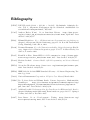
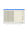
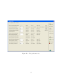
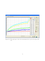
B. Screenshots
55
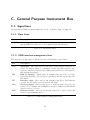
C. General Purpose Instrument Bus
C.1. Signal lines . . . . . . . . . . . . .
C.1.1. Data Lines . . . . . . . . . .
C.1.2. GPIB interface management
C.1.3. GPIB handshake lines . . .
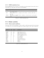
C.2. Global variables . . . . . . . . . . .
C.2.1. Status word conditions . . .
60
60
60
60
61
61
61
D. Activity Diagram: Initialization
. . .
. . .
lines
. . .
. . .
. . .
.
.
.
.
.
.
.
.
.
.
.
.
.
.
.
.
.
.
.
.
.
.
.
.
.
.
.
.
.
.
.
.
.
.
.
.
.
.
.
.
.
.
.
.
.
.
.
.
.
.
.
.
.
.
.
.
.
.
.
.
.
.
.
.
.
.
.
.
.
.
.
.
.
.
.
.
.
.
.
.
.
.
.
.
.
.
.
.
.
.
.
.
.
.
.
.
.
.
.
.
.
.
.
.
.
.
.
.
62
E. Class diagrams
63
E.1. Bus control . . . . . . . . . . . . . . . . . . . . . . . . . . . . . . . . . . 63
E.2. Data management . . . . . . . . . . . . . . . . . . . . . . . . . . . . . . . 64
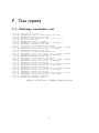
F. Test reports
65
F.1. Discharge transformer test . . . . . . . . . . . . . . . . . . . . . . . . . . 65
F.2. Timer auto adjustment test . . . . . . . . . . . . . . . . . . . . . . . . . 66
3
F.3. Check physics test . . . . . . . . . . . . . . . . . . . . . . . . . . . . . .
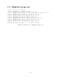
F.4. Weighted average test . . . . . . . . . . . . . . . . . . . . . . . . . . . .
4
67
68
1. Introduction
1.1. Overview
1.1.1. Aim of a transformer test
Transformers are used in nearly every electronic device. They are used for example to
step up or down an alternating voltage or to decouple two electrical circuits. During
this process the transformer heats up due to copper and core losses. The copper losses
are caused by the resistance of the transformer windings whereas core or iron losses are
caused by the recurring reorientation of the magnetic field inside the transformer core
[Spr09].
The single windings of a transformer are made of enameled wire, which is wire coated
with a thin insulating layer. This layer must endure temperatures caused by the heating
of the transformer without melting or decomposing. Transformers are classified into
one out of seven isolation classes according to DIN EN 60601-1 [DIN07, p.56 (42.1)].
These classes guarantee one of the following maximum operating temperatures for a
transformer:
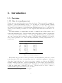
Class Tmax heating
Y
A
E
B
F
H
C
90◦ C
105◦ C
120◦ C
130◦ C
155◦ C
180◦ C
>180◦ C
Tmax overload
150◦ C
165◦ C
175◦ C
190◦ C
210◦ C
-
Table 1.1.: Isolation classes
Each transformer’s isolation class is provided by the manufacturer and can be found
in the data sheet. The aim of a transformer test is to verify the compliance to this given
class after being built into the device it is going to supply, according to the [DIN07]
standard which specifies the “general requirements for basic safety and essential performance of medical electrical equipment”1 . The difference to the manufacturer’s test
is that the transformer is built into the device. This is needed in order to achieve a
certified market approval for the Dräger products.
1
translation found on http://www.vde-verlag.de
5
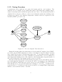
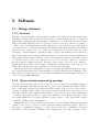
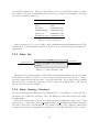
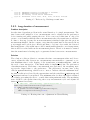
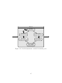
1.1.2. Testing Procedure
A transformer test is split into two parts, the heating and the overload phase. The
ambient, case (cf. chapter 1.4.3), transformer surface and transformer winding temperatures are measured periodically throughout the test. Due to the measurement method
explained below, the precondition to start a test is that the transformer winding’s temperatures are equal to the ambient temperature, which is therefore requested by the
standard [DIN07, p.60 (42.3, 4)].
Adjust settings
Start heating
test phase
Store measurement
data to HDD
Pause test
Test
engineer
Software
timer
Adjust loads
Perform
measurement
Start overload
test phase
Finish test
Export data
Figure 1.1.: Use case diagram: User interaction
During the heating phase the transformer is loaded with 110% supply voltage [DIN07,
p.59 (42.3, 2)] and 110% ampacity (cf. table 1.2 in chapter 1.4.8) according to its data
sheet, until it has reached a steady temperature state. To pass this test phase, the final
temperature must neither exceed Tmax heating as found in table 1.1 nor be limited by
any temperature limiting device. The duration of the heating phase depends heavily on
the tested transformer, but usually it takes a whole work day.
After the transformer has passed this heating test phase, it is loaded with about twice
its normal ampacity during the overload test (cf. table 1.2 in chapter 1.4.8). During this
test especially the transformer’s protective devices are tested [DIN07, p.78 (57.9.1, b)].
Their intention is to prevent the transformer windings to exceed Tmax overload also
found in table 1.1. Possible protective devices would be for example fuses, temperature
limiters, excess current releases or the like.
6
To pass the test for a model series, the tested transformer has to withstand the applied
load either until a protective device triggers, for 30 minutes, or again until a persistent
temperature state is reached. In all three cases, the transformer must not heat up above
the maximum overload temperature listed in table 1.1 [DIN07, p.78 (57.9.1, b)].
Before the test can be started, the test engineer must firstly adjust the preferences
and secondly connect the correct loads and the device under test (cf. section 1.4.3)
properly. These loads need to be readjusted by the user for the overload test to cause a
winding current according to table 1.2. Once started by the engineer, measurements in
both heating and overload phases are initiated periodically by a timer. Further the user
can pause or end the test and export the measured data. This functionality is depicted
in the use case diagram 1.1.2.
1.2. Aims of this work
1.2.1. The need of such a control software
The Dräger TestCenter is one of the accredited IECEE CB2 test laboratories in Germany.
Tests carried out under the CB scheme are accepted worldwide in many countries and
allow several market approvals for a product with a single test [IEC09]. Since the
transformer test is part of the DIN EN 60601-1 [DIN07] and the test reports are generated
according to this standard, it completes Dräger’s in-house testing portfolio.
The alternative of testing the transformers directly inside the Dräger TestCenter
would have been to outsource the tests to an external CB test laboratory. As this
would be disadvantageous with regards to time- and cost-targets compared to in-house
testing, Dräger decided to set up this test stand about 20 years ago. Since 1998 a software originated from a diploma thesis controlled the test stand. It was written in Delphi
1.0 for the operating system Windows 3.11. After the control computer has necessarily
been replaced by a more modern one operating with Windows XP, the existing software was no longer usable and Dräger requested a successor, written in a more modern
programming language.
1.2.2. Requirements
The new software needs to satisfy the following criteria:
• Documentation of all necessary data
This includes reference values, date and time as well as the measurement data.
• Saving measurement values reliably
Data has to be stored in any event to a persistent storage. A loss of data must be
prevented by all means.
2
All used abbreviations are explained in the glossary.
7
• Measuring and storing correct reference values
The ambient temperature and the cold (initial) resistance need to be measured
and stored at the beginning of the test. These reference values have to be correct,
because all further winding temperature calculations are based on them.
• Periodical measurements of temperatures
Throughout the test the winding, ambient, case and transformer surface temperatures need to be measured and stored reliably at regular intervals.
• Using the existing hardware
The existing devices of the test stand (see chapter 1.4) should be used and controlled by the new software as far as this is possible.
• Structured, expandable and understandable source code
The source code and the structure of the new software should be comprehensible to
allow future adaptations by other programmers. In the future it should be possible
to replace the controlled devices (scanner and multimeter) without rewriting an
unnecessary amount of code.
• Robustness and fault tolerance
The software should be robust regarding incorrect user inputs, power failures and
other unpredictable situations. Losing data or storing incorrect measurements
should be prevented as far as possible. Hardware faults should be tolerated and
if possible remedied, provided these faults are known as being temporary. Other
faults should not cause the software to crash or to lose data.
1.3. Robustness and fault tolerance
1.3.1. Definitions
The following definitions of robustness and fault tolerance are taken from the IEEE
Standard Glossary of Software Engineering Terminology [IEE90]. Throughout this work,
these terms are referenced, and it will be shown, that these are applicable attributes for
the Trafotest software.
robustness The degree to which a system or component can function correctly in the
presence of invalid inputs or stressful environmental conditions.
fault (1) A defect in a hardware device or component; for example a short circuit or a
broken wire.
(2) An incorrect step, process, or data definition in a computer program. Note:
This definition is used primarily by the fault tolerance discipline. In common
usage, the terms “error” and “bug” are used to express this meaning.
8
fault tolerance (1) The ability of a system or component to continue normal operation
despite the presence of hardware or software faults.
(2) The number of faults a system or component can withstand before normal
operation is impaired.
(3) Pertaining to the study of errors, faults, and failures, and of methods for
enabling systems to continue normal operation in the presence of faults.
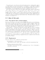
1.4. Test setup
1.4.1. Overview
The test stand consists of seven major devices surrounding the transformer under test.
To supply and load the transformer, an isolation transformer on the primary side and a
variety of different electrical consumers on the secondary side of the device under test
are used.
The arising temperatures are measured with thermocouple sensors for transformer
surface, interior enclosure and ambient temperatures plus an in chapter 1.6.2 described
resistance based measurement method for the transformer winding temperatures.
The controllable devices - scanner and multimeter - are connected via the General
Purpose Instrument Bus to a control computer whose tasks comprise the switching of
the circuits with the scanner, collecting raw data with the multimeter, calculating the
searched temperatures on that basis and check the plausibility of the data afterwards.
1.4.2. Isolation transformer
The isolation transformer is used to power the device under test according to its data
sheet and, at the same time, decouple the test circuit from the supply circuit for safety
reasons.
Used device: Elabo AC Power Supply 35-2J.
1.4.3. Device under test
The transformer to be tested is the device under test (DUT). Supported are transformers
with one primary (input) and up to 5 secondary (output) windings. Throughout the
test the transformer has to be either built-in or placed in a suitable test box that allows
to simulate the heat accumulation while being built-in.
1.4.4. Scanner
The scanner has two important functions: On the one hand it is used for measuring the
sensor temperatures as described below, on the other hand it facilitates the control of
all relays needed to operate the test stand. A detailed circuit diagram with all relays
9
numbered according to their respective scanner channel can be found in Appendix A. It
is controlled completely over the GPIB.
Used device: Hewlett Packard HP 3495 A Scanner
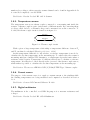
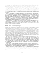
1.4.5. Temperature sensors
The temperature sensors are thermocouples connected to a measuring unit inside the
scanner. A thermocouple is a pair of wires made of different metals. By connecting them,
a voltage called Seebeck - or thermal voltage can be measured across the connection. To
do this, the thermocouple circuit is formed as in figure 1.2.
Metal A
Metal B
T1
+−
T2
Figure 1.2.: Thermocouple circuit
With a given voltage-temperature relationship a temperature difference between T1
and T2 can thus be calculated [Hew83, p.3-19, sec. 3-110].
As this temperature difference is only relative, a reference temperature is needed to
calculate the absolute temperature at the measuring tip. To achieve this, the scanner’s
measuring unit has a built-in NTC thermistor, a temperature dependet semiconductor
resistance with N egative T emperature C oefficient, that allows to calculate a reference
temperature. It is therefore located directly at the open end of the thermocouple sensors,
which makes it possible to calculate the absolute temperature at the measuring tip.
Used devices: Thermocoax 2FKAc10.J.CI1/15/DS40/PTFE Type J thermocouples
1.4.6. Current source
The purpose of the current source is to apply a constant current to the windings while
the winding temperatures are being measured and computed as described in section
1.6.2.
Used device: Siemens DC Current Calibrator D 2302
1.4.7. Digital multimeter
The multimeter is also controlled over GPIB. Its purpose is to measure resistances and
voltages.
Used device: Hewlett Packard HP 3478A Multimeter
10
1.4.8. Loads
To test the transformer’s heating it has to be loaded. These loads can be fan heaters,
halogen lamps or similar electrical consumers and must force a winding current according
to the below table 1.2. The first column is the nominal ampacity that can be found in the
transformer’s data sheet, the other columns give the percentage of the nominal ampacity
the transformer has to be loaded with.
Nominal ampacity
Heating
Overload
<4A
4A - 10A
10A - 20A
>25A
110%
110%
110%
110%
210%
190%
175%
160%
Table 1.2.: Loads
Used devices: Several different ones depending on the needed consumption.
1.4.9. Control computer
A common personal computer with Windows XP as operating system is used to control
the test stand. The GPIB is connected to the computer via a National Instruments
GPIB-USB adapter.
Used device: Microstar PC with Intel Celeron CPU @ 2,53GHz, 256MB RAM, Windows XP
1.4.10. Bus connection
GPIB is the abbreviation for General P urpose I nstrument B us. The control computer
communicates with both scanner and multimeter via this bus. It thereby provides the
ability to operate the devices and to read measurement data from the digital multimeter. A detailed description of the GPI bus follows in section 1.5, whereas the use and
adaptation of the National Instruments API library is explained in section 2.3.1.
Used device: National Instrumens GPIB-USB-HS Adaptor
11
1.5. GPIB Basics
1.5.1. Overview
The GPIB was developed in the late 1960s by Hewlett Packard under the name Hewlett
Packard Instrument Bus (HP-IB). Since 1975, when the IEEE3 first published the ANSI/IEEE Standard 488, the bus has been developed and refined continously and is still
a commonly used bus to connect measurement equipment from various vendors. The
prevailing standard for this work is IEEE 488.1-1987 which is supported by both devices,
scanner and multimeter.
The bus consists of 24 lines: 8 ground lines and 16 signal lines, split up into 5 control
lines, 3 handshake lines and 8 bi-directional data lines. Further details about the GPIB
signal lines can be found in appendix C. Up to 15 devices can be connected simultaniously
to the bus, each uniquely identified by its addresses. GPIB addresses consist of two
parts: a primary and an optional secondary address. For the transformer test stand
only primary addresses are used which are a number in the range 0 to 30. A device can
either be controller, talker, listener or may incorporate more than one of these options.
Nevertheless only one option can be active at a time. Additionally, there is only one
active controller and one active talker allowed at the same time.
GPIB device options
Controller sends formatting or programming commands to the connected devices plus
it makes the individual devices to talk (resp. un-talk) or listen (resp. un-listen).
Talker sends data byte serial to the bus using the 8 data lines plus the data valid (DAV)
handshake line.
Listener receives information from the talker over the 8 data lines. It controlles the not
ready for data (NRFD) and no data accepted (NDAC) handshake lines.
1.5.2. GPIB API library
The software uses a C-library provided by National Instruments (NI) to control the bus.
This API library comes with a header file “ni488.h” as well as a precompiled object
code file “gpib-32.obj”. Although this library is taken from the latest NI Developer
Tools distribution which base on the IEEE 488.2 standard, it can be used for the control
software as this standard is downward compatible to IEEE 488.1.
This library provides besides all single- and multi-device GPIB commands four global
variables which are updated after each API call. These status variables are the status
word ibsta, the error variable iberr, and the count variables ibcnt and ibcntl.
The status word contains information about the state of the bus and the connected
hardware. It is a 16 bit value where each bit represents a certain condition. The most
important one is the error condition. If an error occurs this bit is set and more details
3
IEEE: Institute of Electrical and Electronic Engineers
12
about the error can be found in the error variable iberr. Status conditions and error
details are listed in appendix C. After each send, receive or command function the
variables ibcnt and ibcntl are updated to the number of bytes sent or received. These
variables differ only in their type, where ibcnt is defined as int while ibcnt is a long
int. Therefore the content equals as long as the value is representable by an int.
1.5.3. GPIB commands
To perform all actions needed to control and carry out the transfromer test, the software
uses seven commands of the API library that allow to program the devices, switch the
circuits and read the measured data. This section will give a short description of the used
commands but will ignore implementation and error handling aspects as they are dealt
with in chapter 2.3.1. A detailed description of all GPIB commands can be found in the
Linux GPIB documentation [Hes05]. The information for the following explanations is
extracted from this documentation.
DevClear
A clear command is sent by the board specified by board desc to the device with the
address specified in address. This command causes the device to transit to its idle
state, which means in particular for the scanner, that no switched circuit is conducting.
1
void DevClear ( int board_desc , Addr4882_t address );
Listing 1.1: Usage: DevClear
EnableRemote
EnableRemote() asserts the remote enable (REN) line, and addresses all of the devices
in the addrLst[] array as listeners, which causes them to enter remote mode. The
board specified by board desc must be system controller.
1
void EnableRemote ( int board_desc , const Addr4882_t addrLst []);
Listing 1.2: Usage: EnableRemote
FindLstn
FindLstn() will check the addresses in the addrLst[] array for devices. The GPIB
addresses of all devices found will be stored in the resultList[] array, and ibcnt
will be set to the number of devices found. The maxNumResults parameter limits the
maximum number of results that will be returned, and is usually set to the number of
elements in the resultList array. If more than maxNumResults devices are found, an
ETAB error is returned in iberr.
1
void FindLstn ( int board_desc , const Addr4882_t addrLst [] ,
Addr4882_t resultList [] , int maxNumResults );
Listing 1.3: Usage: FindLstn
13
Receive
Receive() performs the necessary addressing, then reads data from the device specified
by address.
1
void Receive ( int board_desc , Addr4882_t address , void * buffer ,
long count , int termination );
Listing 1.4: Usage: Receive
Send
Send() addresses the device specified by address as listener, then writes data onto the
bus
1
void Send ( int board_desc , Addr4882_t address ,
const void * data , long count , int eot_mode );
Listing 1.5: Usage: Send
SendIFC
SendIFC() resets the GPIB bus by asserting the ’interface clear’ (IFC) bus line. The
board specified by board desc becomes controller-in-charge.
1
void SendIFC ( int board_desc );
Listing 1.6: Usage: SendIFC
Trigger
TriggerList() sends a group execute trigger command (GET) to the device specified
by address, which causes for example the multimeter to perform a measurement and
output the measured data.
1
void Trigger ( int board_desc , Addr4882_t address );
Listing 1.7: Usage: Trigger
WaitSRQ
WaitSRQ() sleeps until either the service request (SRQ) bus line is asserted, or a timeout
occurs. A ’1’ written to the location specified by result indicates that SRQ was asserted,
and a ’0’ that the function timed out.
1
void WaitSRQ ( int board_desc , short * result );
Listing 1.8: Usage: WaitSRQ
14
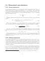
1.6. Measurements and calculations
1.6.1. Sensor temperatures
For receiving the ambient, case and transformer surface temperatures the voltages of
thermocouple sensors, as described in chapter 1.4.5, are measured. The relationship
between the temperature difference and the output voltage is nonlinear, but can be approximated by a polynomial where Trel is the temperature difference, ci the ith coefficient
and u the measured voltage.
N
X
Trel =
ci u i
(1.1)
i=0
With the coefficients taken from the sensor data sheet the 3rd degree polynomial thus
results to
Trel = 1.92101590835 · 104 · u − 1.31196265183 · 105 · u2
+ 4.07065543379 · 106 · u3
(1.2)
The absoulte temperature of the NTC resistance TN T C is computed with an equation
taken from the scanner’s user manual4 using RN T C as measured thermistor resistance.
TN T C =
5041.6
− 314.052;
ln(RN T C ) + 7.15
(1.3)
The sum of both NTC temperature and temperature difference between the NTC
resistance and the measuring tip equals to the absolute temperature at the measuring
tip.
Tabs = TN T C + Trel
(1.4)
These measurements are, in contrast to the ones for the winding temperatures, independent from accessing the DUT’s connectors and can thus be carried out while the
transformer is loaded.
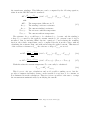
1.6.2. Winding temperatures
The winding temperatures can’t be measured directly with sensors as described above,
because the windings are isolated and thus unreachable for those sensors. The transformer surface temperature under loading is usually lower than the actual winding temperature, as the winding’s heat reaches the surface with a time delay and the surface gives
off heat. For this reason the winding temperatures are obtained using a temperatureresistance dependency.
Provided that the transformer windings are adapted to the ambient temperature
(Tw,ref = Tamb,ref ) at the beginning of the test, and that this reference temperature
as well as the initial resistance of the transformer windings are known, it is possible to
compute a temperature difference between the current and the reference temperature of
4
Hewlett Packard, Model 3495A Handbook, Section III, Page 3-20, Chapter 3-115.b. Equation 1
15
the transformer windings. This difference can be computed by the following equation,
taken from the DIN EN 60601-1 standard5 :
∆T =
Rw,cur − Rw,ref
· (234.5 + Tamb,ref ) − (Tamb,cur − Tamb,ref )
Rw,ref
with
∆Tw :
Rw,ref :
Rw,cur :
Tamb,ref :
Tamb,cur :
The
The
The
The
The
temperature difference in ◦ C
winding’s reference resistance
current winding’s resistance
reference ambient temperature
current ambient temperature
(1.5)
The resistance Rw,cur would have to be calculated, too, because only the winding’s
voltage Uw,cur caused by the applied constant current Iw (cf. current source 1.4.6) is
measured. But by inserting Ohm’s law into equation 1.5 and reducing the resulting
fraction, the relative temperature can be computed directly from the voltage without
calculating the resistance first, and without knowing the applied current. Thus instead
of the reference resistances Rw,ref the reference voltages Uw,ref are stored.
⇔ ∆T
U
Uw,cur
− w,ref
Iw
Iw
=
Uw,ref
Iw
⇔ ∆T =
· (234.5 + Tamb,ref ) − (Tamb,cur − Tamb,ref )
(1.6)
Uw,cur − Uw,ref
· (234.5 + Tamb,ref ) − (Tamb,cur − Tamb,ref )
Uw,ref
(1.7)
With this value the current temperature Tcur can easily be calculated:
Tw,cur = ∆Tw + Tamb,ref
(1.8)
This does not only save calculations and avoid possible rounding errors, but also
provides robustness and fault tolerance, as the current does not have to be constant, as
it is eliminated from the calculations. Therefore it is not possible for the user to corrupt
the measurement unintentionally by modifying the current.
5
DIN EN 60601-1:1990 + A1:1993 + A2:1995, Page 60, Section 42.3 (4)
16
2. Software
2.1. Design decisions
2.1.1. Overview
Writing a robust and fault tolerant software requires a thought out software design. The
handling of an ideal test as described in section 2.4, a test without any error or fault, is
quite simple. Regarding the high quantity of different errors and their various severities
that can actually happen (section 2.5), the problem becomes more and more complex.
First of all, a robust and fault tolerant software has to detect such errors, as undetected
errors may lead to corrupt measurement data which might affect the final test result in
the worst case, or may cost a lot of time for restarting the test in the best case. The
reliability of a test result is not only important to comply some standard, it becomes more
important keeping the devices in mind which are powered by the tested transformers.
These transformers will be built into devices like respirators that lives literally depend
on. With regard to that, error detection is a very serious issue. But once detected,
the error must be handled properly. Because of the variety of errors it is not useful to
handle them all equally. Some require an immediate interruption of the test process
while others should just cause a repetition of the last measurement.
The single most important thing to achieve robustness and fault tolerance is to write
the software as structured and comprehensible as possible right from the beginning. This
approach allows easy bug detection, provides extensibility, and particularly helps not to
overlook programming mistakes.
2.1.2. Object-oriented programming paradigm
The first major design decision was to use an object-oriented programming language
which brings many advantages with regard to the goals robustness and fault tolerance.
One of the main benefits is the understandable transfer from a real world problem to
source code [Erl08]. Every entity of the transformer test stand can be seen as an object,
from the datasets of the single measurements to the electronic devices like multimeter
or scanner. It is thus possible to compare the hardware and software structure of the
test stand which allows together with the following point to locate bugs inside certain
boundaries. This point is encapsulation.
Encapsulation is a very powerful characteristic of object orientation that prevents the
outside of an object to access its inner structure unless explicitly granted. Thereby
the danger of unintended changes of object data is reduced to a minimum. Another
advantage of this information hiding is the transparency. By only accessing objects
17
via interfaces their implementation can be changed without affecting other parts of the
program. This feature thereby makes the code reusable, extensible and robust.
The data that has to be stored in the objects or that the objects consist of can be
categorized by their type. Possible types are for example integer, string or floating point
values. With regard to the robustness of the software, the programming language should
not allow to store values of different types into the same variable, as this might provoke
errors or undefined results if for example an unexpected string is being multiplied with
an integer.
After avoiding many programming mistakes by choosing a language supporting the
above features, there has to be a support for handling errors in an appropriate way. As
mentioned before, different errors need to be treated differently. Some can be solved
inside the capsule where they appeared, others need to be passed to for example to their
calling function or even to higher levels to guarantee accurate handling. An appropriate
treatment of emerging errors is necessary to develop a fault tolerant software, therefore
a programming language with support for exceptions will be used.
Considering all of the previously described aspects, a language that matches these
criteria is C++. This language is used together with the integrated development environment (IDE) Microsoft Visual Studio .NET Version 7.1, 2003 to develop the control
software for the transformer test stand.
2.1.3. State machine paradigm
A finite state machine is “a computational model consisting of a finite number of states
and transitions between those states, possibly with accompanying actions.” [IEE90].
With regard to that model, a transformer test also consists of different states. After
leaving an idle state, the test starts with an initialization and continues with the heating
and the overload phases as described in section 1.1.2. In addition to that, both, heating
and overloading are interruptible and thus have corresponding pause states. After these
phases are run through, the test finishes with the export of the measured data. These
states can be summarized as parts of a finite state machine which gives several important
advantages which will be explained further on.
By using a state machine the complete testing procedure can be depicted by a state
chart. Every state is represented by a C++ class. Together with the encapsulation of
this language, the complexity of the whole project is divided into several less complex
states. These can be seen as self-contained sub-projects which do not affect other parts
of the program without transiting into another state. Owing to such a division, major
programming mistakes can be avoided and - if still made - be located precisely inside
one single state.
The complete software structure can further be designed on paper, understandable to
the end user who doesn’t necessarily need knowledge in the programming language, and
comprehensible to other programmers who maintain the test stand later on.
Source code can become very obfuscated, if a lot of small changes are applied and
reverted back and forth to the initial design. Using the state chart, a change of the
program structure can be discussed preliminary without touching or even knowing any
18
code. The later program flow can be gone through and mistakes can be detected and
fixed before adding the changes to the source code. The result can be a very robust and
well-reasoned concept which in turn leads to a robust software.
2.2. The state machine
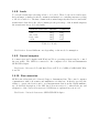
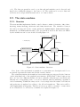
2.2.1. Overview
The state machine implemented in the control software consists of six states: Idle, Init,
Heating, Pause Heating, Overload and Pause Overload. The transition between
the states are triggered by five events: EvInit(), EvShutdown(), EvStartHeating(),
EvPause(), and EvStartOverload(). The program flow and how the states are linked
by the transitions can be seen in the following figure 2.1:
Init
startNewMeasurement()
* := EvShutdown()
EvStartHeating()
*
Pause Overload
restore()
*
Idle
*
*
EvStartOverload()
Heating
*
EvPause()
EvPause()
Overload
restore()
EvStartOverload()
EvStartHeating()
Pause Heating
Figure 2.1.: State machine: Overview
Note: Some of the used function, transition or event names are descriptive and do not
necessarily represent the names used in the actual software.
The events that initiate the transitions between the states are triggered by five buttons
on the right hand side of the graphical user interface (GUI). Each of these buttons can
have one out of two different statuses: It can be enabled so that the user can click it and
thus fire its corresponding event, or it can be disabled whereby initiating a transition
can be hamstrung. Within the entry action of every single state the status of all buttons
and preferences is updated according to the allowed transitions. This action will be
called updateBP() in diagrams. Thereby, it is never possible to transit to a state when
it’s not intended to be allowed by a transition as depicted in figure 2.1.
19
Due to the encapsulation into states, the single states know nothing about the tasks
and actions other states have to perform. When control over the test stand is passed
from one state to another, the new state has no information in what condition the test
stand is passed to it. Therefore it would be difficult for the state to fulfill its task
reliably. There are two possible ways to solve this problem. The first is that every state
performs an initialization by itself that leads to a defined test stand condition. But this
would produce a lot of overhead source code and unnecessarily repeated bus commands
which is why the second solution is better. The idea is to use a contract between the
states defining the test stand condition during the transitions. The connected devices
thus have to be handed over in their idle state. In the unlikely event of an error that
prevents a device from being passed in its idle state, a reinitialization within the target
state would not solve the problem either, which is why the contract is the best solution
for this.
The following section will give an overview about the different states, their purpose as
well as their entry and exit actions with reference to the measurement cycle described
in section 1.1.2.
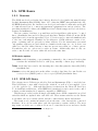
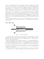
2.2.2. State: Idle
Idle
EvShutdown()
OnEntry / updateBP()
OnExit / EvInit / Initialize + transit
startNewMeasurement()
restore()
Figure 2.2.: State machine: Idle
A transformer test always starts and ends in the Idle state. The entry action enables
all preferences plus the Initialize button, other buttons are disabled. The user actions
within the Idle can be divided into two parts. The first part is to set the preferences,
the second is to initialize the test.
During the initialization after sending an interface clear command (SendIFC(), cf.
1.5.3) it is checked, whether both devices are connected properly and do respond while
performing a FindLstn() call (cf. section 1.5.3). Assuming that the devices respond and
the software was either never started before or ended in idle state after the last run, a
new test will be started. Therefore the reference values Tamb,ref and Rw,ref , introduced in
section 1.6.2, are measured and stored. Now that the software is successfully initialized,
it transits to the Init state.
If the software ran before and did not finish in Idle state, a crash, for example due
to a power failure, can be assumed. In this case the user has the possibility to restore
20
a previously startet test. Thereby the software does not transit necessarily to Init.
According to the state in which the test aborted, the software now transits to the next
safe state as listed in table 2.1.
Last state
Next safe state
Idle
Init
Heating
PauseHeating
Overload
PauseOverload
Idle
Init
PauseHeating
PauseHeating
PauseOverload
PauseOverload
Table 2.1.: Next safe states
States considered to be safe are Idle, Init, PauseHeating and PauseOverload. The
detailed flow of the initialization phase is depicted as an activity diagram in figure D.1,
appendix D.
2.2.3. State: Init
Init
startNewMeasurement()
OnEntry / updateBP() + init output filename
OnExit / -
EvStartHeating()
EvShutdown()
Figure 2.3.: State machine: Init
The Init state’s current task is to inform the user that the initialization was successful.
In the future it will be possible not only to start the transformer test but also to start a
necessary quick check from this state. At the moment the only possible actions within
this state are to change the preferences and to start the heating phase. All buttons
except Start Heating are disabled.
2.2.4. State: Heating / Overload
The states Heating and Overload are summarized to one chapter, because the measurement cycle equals in both states. The only difference is the time between two single
measurements.
The states heating and overload are starting a timer within their entry action. This
timer is set to a preference value (m timeHeating or m timeOverload) that determines
the time between two measurements. The timer regularly calls a function which then
measures the searched temperatures. As this is not only the main task of the software,
21
Heating
EvStartHeating()
OnEntry / updateBP() + startTimer()
OnExit / unloadTransformer() + stopTimer()
OnTimer / measure()
EvPauseHeating()
EvShutdown()
Overload
EvStartOverload()
OnEntry / updateBP() + startTimer()
OnExit / unloadTransformer() + stopTimer()
OnTimer / measure()
EvPauseOverload()
EvShutdown()
Figure 2.4.: State machine: Heating / Overload
but also the one with the most unpredictable situations to handle, it is explained in
detail in the sections 2.4 and 2.5 of this work.
Leaving the Heating or Overload state causes the software to disconnect the device
under test from its power source (1.4.2), its loads (1.4.8) and all other connections.
2.2.5. State: Pause Heating / Pause Overload
Pause Heating
EvPause()
restore()
OnEntry / updateBP()
OnExit / -
EvStartHeating()
EvStartOverload()
EvShutdown()
Pause Overload
EvPause()
restore()
OnEntry / updateBP()
OnExit / -
EvStartOverload()
EvShutdown()
Figure 2.5.: State machine: Pause Heating / Overload
The Pause states have in addition to updateBP() neither specific entry nor exit actions. These states are nevertheless needed for the user to change the loads connected
to the device under test according to table 1.2 in section 1.4.8. Additionally these states
are needed when errors are encountered within Heating or Overload state as the pause
states are the corresponding “next safe states” (cf. table 2.1). Because of the obvious
absence of additional entry actions or bus controls inside the state, the proposition that
these states are safe states has to be proven elsewhere. With regard to the transitions
in figures 2.1 or 2.5 it can be seen that entering the pause states is only possible by
restoring or the event EvPause().
As the restoring transits from Idle to Pause it can be assumed that the connected
devices are in their idle state, too, because both devices were initialized and thus set to
22
idle state during initialization (cf. 2.2.2). In this case the state is safe, as no power or
loads are connected to the device under test.
Transiting from the corresponding measuring state Heating or Overload relies on the
contract that both states unload the transformer within their exit actions (cf. 2.2.1,
2.4).
2.2.6. Transition: Shutdown
EvShutdown()
Idle
Figure 2.6.: State machine: Shutdown
The shutdown transition can be triggered throughout runtime from every state. This
transition leads always to the idle state of the software. It provides the possibility for
the user to export the measured data to a comma seperated values file (.csv) which
can easily be accessed and processed by external spreadsheet programs to generate a
test report. A test which is aborted like this can not be resumed in this version of the
software but this will be possible in future.
2.3. Implementation details
The software source can be split up into four major parts: the graphical user interface
(GUI), the bus control, the data management and finally the state machine. This section
will provide information especially about the last three parts, as the user interface is not
the important point of this work.
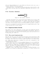
2.3.1. Bus control implementation
The basis of the whole bus control is the library provided by National Instruments. This
C-library allows communication with the bus by calling functions listed in the header
file ni488.h. These functions are described roughly in the NI488.2 User Manual [Nat02,
tab. 7-1ff], whereas their usage is explained very well in the documentation of the
Linux-GPIB package [Hes05].
As this library is provided for the programming language C, it can be included into
the C++ software, but does not comply with the requirements for robustness as introduced in section 2.1. Firstly the error handling with the given library functions is very
elaborate. The NI488.2 User Manual explains how to check for errors after each single
GPIB command. A code example can be found in figure 2.1.
Assuming a usage of the library directly for the bus controlling, this kind of error
handling does not satisfy the requirements as it firstly has to be carried out after every
23
1
5
gpibCommand ( param );
// ibsta : GPIB status word
// ERR :
error bit , defined in ni488 . h
if ( ibsta & ERR )
{
/* error handling */
}
Listing 2.1: GPIB error checking
command which leads to a lot of overhead source code and secondly has to be handled
right away.
Additionally most of the functions have constant parameters if used just for this
one application. Replacing these functions by others with less parameters but same
functionality reduces the risk of unintended errors caused by wrong parameters. This
is also a matter of encapsulation, because the measurement controller should need no
knowledge about the bus controller. An example is the bus interface number which is
in this case always 0 and is needed in every GPIB command.
Another improvement would be to separate the device specific from the common bus
commands. The result of such a separation is extensibility and exchangeability of the
used devices without too much effort, because only a very small amount of code has to
be touched.
By using inheritance the complete common bus control functions are hidden from the
measurement control (cf. section 2.3.4, which then only needs to communicate with the
devices. All other control of the bus happens internally.
The three classes originated from these thoughts and some selected methods are depicted in figure 2.7. A diagram with a complete method list of all classes is located in
appendix E.1.
CBusControl
~CBusControl(void) : void
CBusControl(void) : void
nSend(Addr4882_t addr, std::string sCommand) : void
[...]
CBusDevHP3478A
CBusDevHP3495A
CBusDevHP3478A(void) : void
~CBusDevHP3478A(void) : void
format(enDvmForm format) : void
receive(void) : double
[...]
CBusDevHP3495A(void) : void
~CBusDevHP3495A(void) : void
openChannel(int iCh) : void
openChForIndirResMeas(int iCh) : void
[...]
Figure 2.7.: Class diagram: Bus control (overview)
24
To achieve the desired encapsulation, the library header ni488.h is only included in
the file CBusControl.cpp which makes it impossible for other classes to access the global
variables. Further, all methods of CBusControl are private or protected which allows
only its children to access them. Thus a working bus controller consists of at least one
device, which makes sense in reality, too.
To handle all bus errors the idea of a global status word is replaced by exceptions. If a
device method call fails a for that reason created eBusError can be caught by the calling
function. Thus the error handling is also split into two parts: The error detection is
taken over by the bus controller, and the error handling is transferred to a higher level,
for example the calling function.
An example of the reimplemented methods is how to open two channels (in this
example the channels 31 and 32) with the scanner:
1
5
10
15
# include " ni488 . h "
# define _SCAN 9
/* ... */
SendIFC (0);
if ( ibsta & ERR ) {
/* do error handling */
}
Send (0 , _SCAN , " C31S " , 4);
if ( ibsta & ERR ) {
/* do error handling */
}
Send (0 , _SCAN , " 32 S " , 3);
if ( ibsta & ERR ) {
/* do error handling */
}
1
5
# include " CBusDevHP3495A . h "
/* ... */
CBusDevHP3495A sc ;
try {
sc . openChannel (31);
sc . openChannel (32);
} catch ( eBusError & e ) {
/* do error handling */
}
Listing 2.3: C++ style
Listing 2.2: C style
This example shows how much more comprehensible and easy the C++ style is. Two
main advantages can be extracted from it. Firstly, the measurement controller does not
need to know the device specific commands, as they are only implemented in the device
class. Therefore the device can change without affecting the measurement controller
code. And secondly the error handling can be written down once for many commands
at the end of a code block. The common bus controls are completely hidden from the
measurement controller in the C++ example. Many mistakes as forgotten error handling
or mistyped arguments can thus be prevented. A more robust and through the clarity
easy maintainable software is the result.
Another big advantage of the newly created modularity of the bus control implementation becomes important when it comes to testing or offline developing. By just replacing
the class definition file BusControl.cpp by a dummy file BusControlDUMMY.cpp it is
possible to decouple the program developement from being connected to the real test
stand. Further the return values of all bus functions can be hard coded for testing,
as well as exceptions can be thrown to simulate errors without requiring the hardware.
This will be used a lot in section 2.5, “The real measurement”.
25
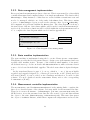
2.3.2. Data management implementation
Every performed measurement produces a data set. This is represented by a class which
contains all measured and computed values of one single measurement. The class is called
CDataSingle. Many instances of this class are created within a transformer test and
need to be managed, which is one of the tasks of the CData class. This class contains
a vector of CDataSingle-objects as well as the reference data object m refDataObj.
All computation is performed within the CData class. The class diagram 2.8 shows a
shortened form of the two data classes which could be used for an ideal measurement (cf.
section 2.4). Several more functions will be added within the real measurement section
2.5 to complete the class diagram which can be found in appendix E.2.
CData
m_dataPacks : std::vector<CDataSingle*>
m_refDataObj : CDataSingle*
[...]
calc_(CDataSingle* obj) : bool
store(CDataSingle* obj) : void
[...]
contains
1..*
CDataSingle
all data variables
[...]
Figure 2.8.: Class diagram: Data management
2.3.3. State machine implementation
The state machine is implemented using the boost C++ library boost::statechart.
This library provides the needed parent classes to design a very well structured and easy
readable state machine in C++. Because of the relatively small number of six states,
all declarations are pooled in one header file CStateMachine.h, while each state classes
source code is located in individual .cpp files. The whole state chart is depicted in figure
2.9.
As the statechart library is part of boost.org, which is “...one of the most highly
regarded and expertly designed C++ library projects in the world” [SA04] and very
well tested [Riv07], it can be relied on its robustness and therefore be used for this
software. For more details about the statechart library refer to the corresponding
documentation [Dön07].
2.3.4. Measurement controller implementation
The measurement controller CMeasurementControl is the missing link to complete the
three above described parts of the software. It is responsible for the measured raw data.
Therefore it creates an instance of CDataSingle, performs a measurement using the
GPIB devices, stores the measured raw data into the created object and then returns
the object to the state (CStateHeating or CStateOverload). This state then passes
the object to its CData instance, which then computes all temperatures and stores the
26
CStateMachine
boost::statechart::state_machine
boost::statechart::state
CStateIdle
CStateHeating
CStateInit
CStatePauseHeating
CStateOverload
CStatePauseOverload
Figure 2.9.: Using the boost::statechart library
object in its data set vector m dataPacks. Figure 2.10 shows an overview how all the
above described classes are associated.
CStateHeating
CBusDevHP3478A
1
1
1
CDataSingle
CData
1..*
CStateMachine
1
1
CMeasurementControl
1
1
CStateOverload
1
CBusDevHP3495A
Figure 2.10.: Class diagram: Software overview
2.4. The ideal measurement
As mentioned in the design decisions overview 2.1.1 the execution of an ideal measurement is quite simple. It requires no error handling and returns always the correct result.
This model will help to understand the crucial points of the measurement procedure
with focus on the implementation. But this ideal process can and will be disturbed by
external influences within a real measurement, which is described in section 2.5.
27
2.4.1. Preconditions
An ideal measurement has certain preconditions which differentiate it from the real
measurement. These requirements are listed as follows:
No time delays. There may be no time delays at all. The transformer has to load and
unload immediately after being connected, the measurements take no time, every
bus command is carried out promptly, and so on.
Reliable measurements. All measured values must be correct within certain boundaries. There must be no statistical outliers, which implies a correct functioning
hardware.
Reliable devices. Both devices, scanner and multimeter, must neither crash nor be
switched off by the user during the test run. Every command sent to them has to
be carried out exactly as expected. The execution of a command takes no time
and happens directly after being called without any delay.
Reliable power supply. The power supply may not cut off or vary its power unless explicitly and intendedly commanded by the control computer. A de- or reconnection
to the device under test may not cause current overshoots that might trigger fuses.
Reliable control computer. The control computer must never crash, been cut off its
power supply, or cause the software to interrupt in any other way. The hard disk
must provide enough space for all measured data and may never fail. Data on
the hard disk that has to be accessed by the software must always be read- and
writable and never be corrupted.
Reliable user. Everything has to be connected in the right way. The preferences have to
be set correctly and nothing must be done that endangers the measurement. This
includes, that no devices must be disconnected while measuring, the correct loads
have to be connected to the device under test at all time, and the transformer has
to be adapted to the ambient temperature before the test.
Assuming all of the above prerequisites, an ideal measurement can be performed.
2.4.2. Test procedure
Initialization
As this is an ideal measurement, most of the paths in activity diagram D.1 become
useless, as they are used for error handling only. After initializing the bus, it can
be jumped directly to the “start test” activity. During the initialization a SendIFC()
command is sent to the bus whereby the control computer becomes controller in charge.
Then both connected devices are reseted to their idle state by sending a DevClear()
command to them. Both bus and devices are now ready to use.
28
Measure
references
Initialize
Change
loads
Start
timer
Start
timer
Measure
Measure
Stop
timer
Stop
timer
Export
data
Figure 2.11.: Ideal measurement: test procedure
Measure references
The next step is to measure, calculate and store the reference data which includes the
winding voltages and the ambient temperature. Except that the winding temperatures
can’t be calculated, yet, the measurement is performed exactly as described in the
Measure section below.
Start timer / Stop timer
The timer is a countdown starting at either m timeHeating or m timeOverload depending on the test phase, which initiates the measurement cycle each time the clock runs
out.
Measure
When triggered by the timer, the measurement cycle depicted in figure 2.12 is entered.
Measure
Get sensor
temperatures
Wait until
timer runs out
Disconnect
supply and loads
Reconnect
supply and loads
Get winding
temperatures
Figure 2.12.: Ideal measurement: measuring cycle
The state machine’s measurement controller is used by the measuring state1 to receive
a CDataSingle object which contains the voltages measured by the multimeter. For
measuring the winding voltages they have to be cut off power and loads. The object is
1
The states CStateHeating and CStateOverload are meant by “measuring states”.
29
then passed to the state machine’s CData instance. Within CData, all temperatures are
computed out of the voltages and the reference values, and then added to the object.
After pushing this object to the m dataPacks vector, the device under test is reconnected
to both, supply voltage and loads, and thus continues to heat up until the timer runs
out again or the test is paused or aborted by the user.
Change loads
Between the heating and the overload phases of the test the loads have to be adjusted
as described in section 1.4.8.
Export data
With the end of the transformer test, all data collected during the measurement cycles is
exported from the program and saved to the computer’s hard disk. Now the application
can safely be terminated.
2.5. The real measurement
A real measurement is distinguished by several faults and errors that violate the conditions previously assumed for the ideal measurement. This section exemplifies these
faults, describes the developed solutions as well as their implementations to make the
control software fault-tolerant. The robustness of these implementations is proven by
several tests also presented in this section.
2.5.1. Discharging the transformer
In a real measurement a time-dependent problem is the discharging of the device under
test.
Problem description
When the transformer is disconnected from the power supply, the windings aren’t discharged immediately. Voltage and current inside the windings follow exponential funcL
. Only after about tend = 5·τ all
tions, whose courses depend on the time constant τ = R
variables have reached their approximate final value [Pre07, p.132]. Thus measuring the
voltages immediately after disconnecting the transformer might lead to unpredictable
results because of the still existing residual voltage.
Solution
The problem is solved by waiting until the transformer is discharged before measuring
the voltages. The waiting time has to be set in the preferences to a value between 0ms
and 20000ms by the test engineer. To avoid an unnecessary cooling of the transformer,
30
Model
Type
MK06162
S18142c
RSO 861385
RTO 861410
Isolating transformer
Autotransformer
Toroidal core transformer
Toroidal core transformer
Table 2.2.: Used transformers
Transformer
Winding
L/mH
R/Ω
τ
tend /ms
MK06162
S18142c
S18142c
S18142c
S18142c
RSO 861385
RSO 861385
RTO 861410
RTO 861410
primary
0-110V
0-200V
0-230V
0-245V
primary
secondary
primary
secondary
176.5
271.4
760.2
1056.2
1180.4
260.2
3995.9
468.7
2271.2
0.103
0.63
1.288
1.547
1.643
0.172
3.281
0.284
2.182
1.714
0.431
0.590
0.683
0.718
1.513
1.218
1.650
1.021
8567
2154
2951
3414
3591
7564
6089
8252
5103
Table 2.3.: Transformer inductances
this time should be as small as possible, which is why this value can be adjusted and is
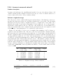
not fixed to 20 seconds. In order to specify the range for the adjustment the inductances2
and resistances3 of the four transformers listed in table 2.2 have been measured and the
resulting τ and tend calculated. The results are written down in table 2.3.
Listing 2.4 shows how the waiting process is implemented in the software. Each
time before the measurement cycle is entered the program waits for the transformer to
discharge.
1
void CM e a su r e me n t C on t r ol :: unloadTrafo ( void ) {
m_pScanner - > closeChannels ();
Sleep ( PREF - > getTimeDischarge ());
}
Listing 2.4: Discharging delay
Test and validation
To test if the software really waits for the configured time a debug output as shown in
listing 2.5 should be enough. A complete log of a test, where it can be seen that waiting
works in both cases, initial and regression measurements (cf. section 2.5.4f) is located
in appendix F.1.
2
3
Inductances were measured with instek LCR Meter LCR-817.
Resistances were measured with Fluke Multimeter 8840A.
31
10
15
...
15:05:08:
15:05:13:
15:05:13:
15:05:13:
...
TESTOUTPUT waiting for transformer to discharge ...
TESTOUTPUT transformer discharged ...
Successfully created initial measurement :
Measurement stored : 24.46 , 24.46 , 24.46 , 24.46094 , 24.46094
Listing 2.5: Trafotest log: Discharge transformer
2.5.2. Long duration of measurement
Problem description
Another time dependent problem is the actual duration of a single measurement. The
time between the initiation of two measurements can be adjusted in the preferences
before starting and while pausing the test. If for some reason this time is only a bit
greater or even smaller than the time a measurement takes, the transformer would have
no time to heat up, because the new measurement is initiated right after the previous
measurement finished. On the contrary, every time the transformer is disconnected from
power supply and loads it gives off heat and thus cools down. As a result, the detected
final temperature of the transformer could be much smaller than the correct temperature
that would be reached without the measurement phases. Therefore it must be ensured
that the transformer is heating up for a guaranteed time between two measurements.
Solution
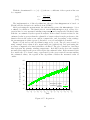
The solution to this problem is to measure the time a measurement takes and, if necessary, adjust the time between two measurements automatically to guarantee a certain minimum time for the heating of the transformer, m minHeatingTime, without
the need of user interaction. This functionality is implemented into the preferences
class CPreferences. Each time a measurement was performed, the measuring state
reports the elapsed time to the preferences. The preferences, in turn, have a flag
called m updateTimerFlag, which is set to true to indicate that the minimum heating time condition is violated by the current timer and the variables m timeHeating and
m timeOverload have been updated. The minimum value for these variables is adjusted
accordingly, preventing the user to override this setting unintentionally. The measuring
state checks for the update timer flag after every measurement cycle and adjusts its
timer m pTimer if necessary.
1
5
/* in function : CStateHeating :: operator ()( void ) */
PREF - > r e p o r t M e a s u r e m e n t T i m e ( elapsedTime );
if ( PREF - > updateTimerFlag ()) {
m_pTimer - > restart ( PREF - > getTimeHeating ());
PREF - > s et Up da te Ti me rF la g ( false );
}
Listing 2.6: Heating time auto adjustment in CStateHeating
32
Test and validation
Prior to each test all preferences are automatically set to default and then adjusted to
the test. In this case the important values are as follows:
• m timeHeating: 30 seconds
• m timeOverload: 40 seconds
• m minHeatingTime: 10 seconds
• m timeDischarge: 0 seconds
All times could be set to anything else within the allowed ranges, but the test set is
created only for these settings. A discharge time different from zero would have to be
added to the sum elapsedSum which is explained below.
Long measurements can be simulated by adding Sleep(x) commands to the GPIB
nReceive(Addr4882 t addr) function inside BusControlDUMMY.cpp (cf. section 2.3.1).
Let elapsedSum be the sum of duration of the measurement elapsedTime and the
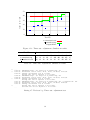
minimum heating time. With this, the test set comprises 10 values covering each of the
following possible situation:
1. elapsedSum ≤ m timeHeating and elapsedSum ≤ m timeOverload
If the above sum is smaller than both timer variables, no update is expected. This
is tested by the tests with ID 1, 2, 3, 5 and 10 to check the correctness before,
between and after the next two test situations.
2. elapsedSum > m timeHeating but elapsedSum ≤ m timeOverload
If the sum is only greater than the smaller of the two timer variables, in this case
the time in heating phase, only this variable should be updated and the other one
should remain untouched. To check whether the expected update occurs only at
the expected point, the simulated duration rises slowly to the update point. This
is tested at the IDs 2, 3 and 4, as well as 6, 7 and 8.
3. elapsedSum > m timeHeating and elapsedSum > m timeOverload
While updating the smaller of the two timer variables, elapsedSum is rising to the
point where both timer variables are expected to be updated. The tests with ID
6, 7, 8 and 9 show the correctness of this situation.
As both m timeHeating and m timeOverload are implemented equally they can be interchanged within this test, wherefore testing the situation elapsedSum ≤ m timeHeating,
but elapsedSum > m timeOverload is not necessary.
Figure 2.13 shows a plot of the 10 simulated durations and the according automatically
adjusted variables listed in table 2.4. The value of the variable m timeHeating is depicted
by the red line, m timeOverload by the green one and the simulated values by the blue
pluses. The offset value m minHeatingTime is depicted by arrows. These arrows are only
plotted if any of the timer variables has been updated.
A complete log of the test is set out in appendix F.2 hereto.
33
50
value in seconds
40
30
20
10
0
0
2
4
6
Test ID
8
10
m timeOverload
m timeHeating
elapsedTime
Figure 2.13.: Timer auto adjustment: Simulation results
Test ID
1
2
3
4
Simulated duration 10
m timeHeating
30
40
m timeOverload
19
30
40
20 21
30 31
40 40
5
6
15 29
31 39
40 40
7
30
40
40
8
9
10
31 35 15
41 45 45
41 45 45
Table 2.4.: Timer auto adjustment: Simulation results
28
30
35
40
...
16:42:55: TESTOUTPUT Slept : 29 s . Expected : m_timeHeating : 39 s
16:42:55: Measurement stored : 24.46 , 24.46 , 24.46 , 24.46094 , 24.46094
16:42:55: Warning : Measurement took 29 seconds !
Heating time will be adjusted to 39 seconds .
16:44:04: TESTOUTPUT Slept : 30 s . Expected : m_timeHeating : 40 s
16:44:04: Measurement stored : 24.46 , 24.46 , 24.46 , 24.46094 , 24.46094
16:44:04: Warning : Measurement took 30 seconds !
Heating time will be adjusted to 40 seconds .
16:45:15: TESTOUTPUT Slept : 31 s . Expected : m_timeHeating : 41 s , m_t imeOverl oad : 41 s
16:45:15: Measurement stored : 24.46 , 24.46 , 24.46 , 24.46094 , 24.46094
16:45:15: Warning : Measurement took 31 seconds !
Heating time will be adjusted to 41 seconds .
Overload time will be adjusted to 41 seconds .
...
Listing 2.7: Trafotest log: Timer auto adjustment test
34
2.5.3. Incorrect measured values I
Problem description
Even if the measurement cycle is performed correctly, the measured data may contain
outliers besides the usual noise. These outliers are most likely caused by unreliable
hardware such as failing relays, but the error has not been located precisely yet. It
happens at completely irregular intervals and can thus falsify successive measurements
as well as measurements which lie far apart. Usually these errors do not affect the test
result, because, as explained in section 1.1.2, the important value is the final temperature
which is measured more than once while being in the persistant temperature state.
But nevertheless removing all the wrong data manually for a test report afterwards is
elaborate for the test engineer and thus costs time and money. But in the worst case
this fault might even affect the complete test result if the reference measurements fails.
As every single winding temperature is computed using the reference data (cf. section
1.6.2), all following calculated values would be wrong and the test would have to be
repeated completely, costing a lot of time. Therefore it is important that those outliers
are detected and handled by the software. Up to now, this fault occurs only while
measuring the primary winding voltage, but with regard to possible future errors and
the long time this software is going to be used, an outlier detection has to be performed
for each measured value. This detection is separated into three different parts, currently
all implemented within the CData class. The first mechanism is a check, whether the
measured values are physically reasonable, the second one an algorithm that computes
a weighted average, and the third one an algorithm that uses a regression analysis to
estimate the next value.
The improvement achieved by these algorithms is exemplified in figure 2.14. A complete transformer test was performed, including heating and overload phase. The validation of measured data was activated and the saving of invalid data sets was enabled.
Therefore the temperature course with and without error detection could be reconstructed with the export file. The thick red line in figure 2.14 is the raw data without
any error handling. The green line shows the result after remeasuring physically incorrect values and the third, blue line shows the function course after remeasuring every
value rejected by check physics, weighted average and the regression estimation. More
details on these plots are given in the following sections.
Solution: checkPhysics()
Some of the measured data sets are outliers that deviate strongly from the correct values.
Therefore, after the temperatures are computed by the software, every CDataSingle
object is checked for physical correctness. If any of the calculated temperatures is below
or equal absolute zero (-273.15 ◦ C) or the measured NTC resistance is negative, the
measurement is rejected by this function. By using the voltages measured to calculate
the winding temperatures and by knowing the applied current from the preferences, it is
also possible to check whether the winding resistances are positive. As by Ohm’s law the
resistance is computed by dividing the voltage by the current, the resistance is positive
35
Temperature of
primary winding in ◦ C
100
50
0
-50
-100
-150
-200
-250
0
:3
16
0
:0
16
0
:3
15
0
:0
15
0
:3
14
0
:0
14
0
:3
13
0
:0
13
0
:3
12
0
:0
12
0
:3
11
0
:0
11
Time
without error correction
+ check physics
+ weightedAvg + regression
Figure 2.14.: Comparison of error detection algorithms
if both current and voltage signs are equal. A rejected measurement is, depeding on the
settings, either remeasured, deleted or stored and marked as invalid.
Test and validation: checkPhysics()
A test set within BusControlDUMMY.cpp returns the valid values RN T C = 2000Ω, Uamb =
Ucase = Utraf o = −0.170mV which lead to Tamb = Tcase = Ttraf o = 24.46◦ C, and Uprim =
Usec = 5mV . After performing three initial measurements (cf. section 2.5.4), within
each measurement cycle one of these values is returned corrupted, causing a rejection of
the measurement by the checkPhysics() function. First RN T C is set to −0.001, which
should be rejected as well as the resultant ambient, case and transformer temperatures.
Within the next three measurements successively each sensor temperature is forced to
a value lower than absolute zero (−273.5◦ C) by returning the voltage −13.82mV . The
next two corrupted return values are negative resistances (−0.8Ω) for the primary and
secondary windings. The complete test report with the six above described rejected
measurements is located in appendix F.3.
23
25
30
...
16:28:54:
16:28:54:
16:28:54:
16:28:54:
16:28:54:
16:28:54:
...
TESTOUTPUT U_amb = -0.01382 = > T_amb = - 273.5: Only T_amb fails .
Rejection cause : Ambient temperature < absolute zero : [ -273.555966]
Warning : Measurement ( UID : 18) rejected by v a l i d a t e _ a n d _ s t o r e ()
TESTOUTPUT U_case = -0.01382 = > T_case = - 273.5: Only T_case fails .
Rejection cause : Case temperature < absolute zero : [ -273.555966]
Warning : Measurement ( UID : 19) rejected by v a l i d a t e _ a n d _ s t o r e ()
Listing 2.8: Trafotest log: Check physics test
36
2.5.4. Incorrect measured values II
Problem description
As figure 2.14 indicates, the checkPhysics() method does not solve the problem of all
outliers. In this specific example it detects even only one of the 18 outliers, wherefore a
better solution is needed to detect outliers reliably.
Solution: weighted average
The only way to detect outliers without previous knowledge of the function course is to
measure the values more than once and then calculate the correct value. The algorithm
that has been developed uses a weighted average to compute the correct value. In a
nutshell, the weight of each value is the number of the neighborhoods of other measurements that overlap with its own one. The size of the neighborhood is determined by a
value m tolerance that can be adjusted in the preferences by the test engineer as well
as the number of measurements to be considered for the decision.
Figure 2.15 and table 2.5 show a set of example data assuming a 1.0% tolerance to
depict how the algorithm works. The size of the dots represent the calculated weight,
the horizontal error bars represent the neighborhood of each value, and the thick red
line the computed result. For each measurement it is checked, whether its neighborhood
overlaps with the neighborhoods of the other measurements. If so, both measurements
are added to a variable globalSum and a counter for the number of added measurements,
representing the sum of all weights, increases by two. The number of times each value
is added to the sum equals the number of measurements whose neighborhoods overlap
with the value’s neighborhood. The algorithm returns either the result of the weighted
average, which is calculated by dividing the weighted sum by the sum of all weights,
or the value UNDEFINED, if the algorithm was unable to decide which values were the
correct ones.
ID
lower limit
= 0.99 · value
value
1
2
3
4
5
0.0309474
0.0311058
0.0308682
0.0292248
0.0303633
0.03126
0.03142
0.03118
0.02952
0.03067
upper limit
weight
= 1.01 · value
0.0315726
0.0317342
0.0314918
0.0298152
0.0309767
3
2
3
0
2
Table 2.5.: Weighted average: limit caculations
(3 · 0.03126 + 2 · 0.03142 + 3 · 0.03118 + 0 · 0.02952 + 2 · 0.03067)
10
= 0.03115
37
(2.1)
result = 0.03115
Measurement ID
5
4
3
2
1
0.03142
0.03126
0.03118
0.03067
0.02952
Voltage
Figure 2.15.: Example: Weighted average
Test and validation: weighted average
With regard to four almost complete transformer tests, a total of 1249 (384, 208, 351,
306) measurements were taken, containing 51 (4.08%) outliers (14, 8, 15, 14). Because
the four tests were performed with two different transformers at four different dates
(2009-10-29, 2010-01-18, 2010-01-20, 2010-03-04), and the almost equal frequency of
error occurance (3.65%, 3.85%, 4.27%, 4.58%), a uniform distribution of the outliers can
be assumed. The developed algorithm has four possible outcomes:
1. Correct result: All values are correct, which means that their neighborhoods
overlap.
2. Correct result: At least two values are correct, while the others are completely
independent from another and thus don’t overlap with any other value.
3. Wrong result: At least two incorrect values overlap, which are therefore not
detected as outliers.
38
4. No result: No neighborhoods overlap at all. Algorithm returns UNDFINED4 to
indicate that no decision could be made.
Assuming a uniform distribution of the outliers, the probability of a correct result for
three taken measurements is 99.51% as calculated in equation 2.2. Considering the
worst case, in which all incorrect measurements’ neighborhoods are overlapping, the
probability for an undetected wrong result is only 0.49%. But in the usual case this
already small percentage is split up into one part of detected fails, where all three
measurements differ and don’t overlap, and one part where a failure really remains
undetected. For example in the 2010-03-04 test, only 5 out of the 14 outliers had
neighbors, which can again be split up into two neighborhoods (0.001245, 0.001244,
0.001242) and (0.00063, 0.000633), while the other 9 values have no neighbors at all and
thus the part with undetected failures is even smaller than the one where the error is
detected, and the data just has to be remeasured to receive a correct result. Once again,
a log of the complete test is located in appendix F.4.
3
P (”3 correct, 0 incorrect”) =P3,0 =
· (0.0408)0 · (1 − 0.0408)3 = 88.25%
0
3
P (”2 correct, 1 incorrect”) =P3,1 =
· (0.0408)1 · (1 − 0.0408)2 = 11.26% (2.2)
1
P (”Correct result”) =P3,0 + P3,1 = 99.51%
P (”Wrong result”) =1 − P3,0 − P3,1 = 0.49%
Even if the probability of error occurrence is sized up to 10%, the probability for
undetected wrong results is, analogously to the above calculation, still less than 3.8%.
Nevertheless, the possibility of a failure still exists, wherefore the important reference
measurement has to be approved by the test engineer. The display of this reference
data is not only important, because the algorithm might fail, but, as this is the first
measurement of the test, it is also possible for the user to recognize mistakes within the
test setup.
To test this algorithm, a test set including 12 values in 4 groups has been created.
These groups comprise each of the four above described outcomes. Only one of the
measured values needs to be tested, because the implementation of the algorithm handles
all values equally. Therefore it doesn’t matter, whether any sensor temperature or any
winding voltage is tested. This test bench, listed in table 2.6, is written for the ambient
temperature.
4
UNDEFINED equals -999.0 and is set via a preprocessor command. The value -999.0 can never be
written to any value because of the checkPhysics() function and can thus be used to indicate an
undefined value.
39
first value
second value
third value
-0.014000
-0.000169
-0.000169
-0.013000
-0.000001
-0.000171
-0.004000
-0.000170
-0.000100
-0.000170
-0.000169
-0.013010
expected result
No result: not decidable
Correct result: 3/3 neighbors
Correct result: 2/3 neighbors
Wrong result: 2/3 outliers
Table 2.6.: Weighted average: Simulation
2.5.5. Incorrect measured values III
Problem description
Although the weighted average algorithm works very reliable, its biggest disadvantage is
the duration of the multiple measurements. For every measurement the transformer has
to be disconnected from loads and supply voltage and thus cools down. Regarding the
865 taken measurements from the 2010-01-18, 2010-01-20 and 2010-03-04 transformer
tests, a single measurement takes always seven or eight seconds, if only one secondary
winding is connected and measured. When connecting additional windings the measurement time increases by two to three seconds per winding. Assuming the usual case
where only one secondary winding is being measured, the weighted average algorithm
takes about 24 seconds to complete.
60
primary winding
Temperature in ◦ C
55
50
45
40
35
30
25
20
0
0
0
:0
14
:0
13
:0
12
0
:0
11
0
:0
10
0
:0
09
0
:0
08
00
:
07
Time
Figure 2.16.: Warming and cooling of a transformer
Within the (2009-10-29) transformer test, plotted in figure 2.16, the transformer was
heated to about 55◦ C and then disconnected from the loads. Its primary winding cooled
40
down from 54.73◦ C (08:22:46) to 51.34◦ C (08:27:46) within the first five minutes. Assuming an almost linear temperature course, the transformer would give off more than
0.3◦ C during the 28 seconds the measurement took. Considering five earlier data sets, the
temperature went up by about 1.68◦ C within five minutes. Because of the exponential
temperature course it can be said, that the warmer a transformer is, the slower it heats
up when it is loaded, and the faster it cools down when it is disconnected from the loads.
Therefore the time a measurement takes has to be smaller than the time the transformer
is loaded, and thus the weighted average algorithm and its related measurements would
be too slow for a heated up transformer.
Solution: regression line
As it can be seen in figure 2.16, for a small period of time, the function course can be
approximated by a linear function. This characteristic is used for the regression line,
which provides the needed faster solution to detect outliers. With the knowledge of the
previous function course, a linear model according to the method of least square errors
can be approximated and thereby the next measured value can be estimated. In this
section only the three point regression is discussed, but nevertheless, using more function
values is possible up to a certain limit and works analogous to the method described
here.
To compute the three point regression line, knowledge of the last three function values
is needed. These data sets, called the initial measurements, are measured and computed
by the weighted average algorithm as described above. To fit a linear function to the
measured values, the method of least mean square errors in equation 2.3 is used, where
m and b are the coefficients of the regression line y = m · x + b.
S=
n
X
(m · xi + b − yi )2 → min!
(2.3)
i=1
Zeroing the partial derivatives gives the normal equations
and
n
P
∂S
= 2·
(m · xi + b − yi ) · xi = 0
∂m
i=1
n
P
∂S
= 2·
(m · xi + b − yi ) = 0.
∂b
i=1
For easier readability the sum
n
P
(2.4)
(2.5)
a is simplified to [a]. With this, the linear system of
i=1
equations that has to be solved looks as follows:
n [x]
[x] [x2 ]
b
[y]
·
=
.
m
[xy]
41
(2.6)
With the determinant D = n · [x2 ] − [x]2 the two coefficients of the regression line can
be computed:
m=
b=
n·[xy]−[x]·[y]
D
[y]·[x2 ]−[xy]·[x]
D
(2.7)
(2.8)
The implementation of this algorithm into the new class CRegression is based on
[Her00] and the derivation is extracted from [NSB05].
After performing the measurement, the current state passes the CDataSingle object
to CData for validation. The function bool valid (CDataSingle* obj) creates a regression line for every measured winding temperature, and compares the calculated value
with the one estimated by the regression analysis. If the relative deviation related to the
estimated value is greater than the adjustable tolerance taken from the preferences, the
function detects the value as an outliers, returns false, and, depending on the settings,
the measurement is either repeated, discarded or stored and marked as invalid.
Figure 2.17 shows how the algorithm is supposed to work. The plot was created by
using example data, taken from a transformer test (2010-01-20), and performing the
necessary computation by hand with Microsoft Excel. The plot contains two data lines
that represent the primary winding temperature. Red filled circles show the actually
measured data whereas the green circles depict the estimated value. If the measured data
lies outside the 3% tolerance range, represented by the green vertical bars surrounding
the estimated values, the regression line algorithm considers the measured value as
outlier.
60
Temperature in ◦ C
55
50
45
40
35
measured value
estimated value
outliers
30
25
0
:3
12
5
:2
12
0
:2
12
5
:1
12
0
:1
12
5
:0
12
0
:0
12
5
:5
11
0
:5
11
5
:4
11
0
:4
11
5
:3
11
0
:3
11
5
:2
11
Time
Figure 2.17.: Regression
42
In the standard configuration, all measurements rejected by one of the above algorithms are discarded and remeasured three times. If the third measurement fails, too,
the data is stored and marked as invalid, thereby conclusions about the cause of the
failure can be drawn after the test by the user. These invalid data sets are skipped while
collecting data for the regression line. If more than two invalid data sets have to be
skipped, the algorithm throws an exception that causes the measuring state to perform
new initial measurements. This becomes necessary especially if the loads and thereby
the winding currents change. For example if a load as a halogen lamp is defective, the
test engineer changes the loads within a measuring state or the loads are disconnected
unintentionally, the slope of the temperature function changes significantly. In this case,
the edge in the function course would cause the regression line algorithm to fail, wherefore the detection of this error as well as the appropriate handling of it, namely the
switch to initial measurements, is important.
Test and validation: regression line
To validate the functionality of the regression line a test set containing 65 specific return
values has been created that comprises all of the following situations. The data taken
during the test run has been plotted in figure 2.18 using the same style as the above
described figure 2.17.
55
Temperature in ◦ C
50
45
40
35
30
25
measured value
estimated value
outliers
20
15
0
:2
01
18
:
01
43
6
Figure 2.18.: Regression
:1
01
4
:1
01
10
12
:
01
:
01
8
:0
01
06
:
01
Time
• A measured value lies within the estimated range and is therefore considered to
be valid.
• An outlier is situated below the expected range and is marked as invalid. The
measurement is repeated and the taken data lies within the range. The invalid
measurement has to be ignored for further regression lines. (01:08:28)
• The temperature begins to rise faster, because for example more loads were connected by the test engineer. Thereby the measured value lies above the estimated
range. As this value is the correct one, both repeated measurements lie also outside
the expected range. The regression line is not able to solve this problem, therefore
it throws an exception that causes three new initial measurements. (01:09:48 01:10:49)
• An outlier lies far below the expectation, even too low to be plotted in an acceptable
temperature range. Remeasuring solves the problem. (01:12:49)
• The transformer cools down, for example because of defective loads. The situation
is almost the same as above, but the measurements are situated too far below the
expected value, and new initial measurements are the consequence. (01:14:09 01:15:09)
• The measured temperature is higher than expected and therefore remeasured.
(01:17:09)
2.5.6. Power failure
In case of a power failure, all data would be lost if not saved to a persistent storage. Therefore, the measurement cycle is extended by one step, in which the measured data is stored to the hard disk after each measurement. An automatically generated name is used for the output file. It consists of the date and time in the format
YYYYMMDDhhmmss.trt, where Y represents the current year, M the month, D the day, h
the hour, m the minute and s the second. The file extension .trt is used to identify
a transformer test file. In case this file is not readable, the Trafotest software just
appends a “ 0001.trt” to the filename and increments this number if the error persists.
Therefore, it is guaranteed, that the measured data is stored to the hard disk unless it
is full or defective. If the software does not finish in idle state, this can be detected, and
the user is asked within the following initialization (cf. appendix D), whether he wants
to restore the data from this file. Thereby it is possible to resume a transformer test.
44
Measure
Get sensor
temperatures
Wait until
timer runs out
Disconnect
supply and loads
Reconnect
supply and loads
Get winding
temperatures
Store measured
data to HDD
Figure 2.19.: Real measurement: extended measuring cycle
45
3. Conclusion and Outlook
3.1. Future Work
The software Trafotest is currently in an alpha state. Many of the occurring errors
can be detected and most of them can be automatically remedied. With the default
set up it should be possible to perform most of the tests properly, only in unforeseen
circumstances the user might have to adjust values for the algorithms. These algorithms,
developed especially for the outlier detection, are working well in all tested cases, as it
can be seen in figure 2.14.
But nevertheless, even if the software is working well in its current state, there is room
for improvements. Major points for that are a graph pane, which shows the temperature
versus the time while performing a test. This will increase not only usability but will
also help to detect mistakes in the test set up easier. Additionally a schematic tab is
in development, where the test engineer can always see which connections are carrying
current at a time. This pane will allow the user also to control each single channel of
the scanner individually, which is very helpful to locate hardware errors.
To ensure that the temperature sensing is working properly, the implementation of a
quick check has already been prepared, as well as the possibility to reopen the .trt files
that contain the whole serialized data of a test, which makes it possible for the user to
resume a test manually. Up to now this is only possible if the software did not shut
down properly, for example after a power failure.
Together with these future improvements, a final version of Trafotest can be created
which is both, robust and fault tolerant with regards to all the in chapter 2 described
implementations and their advantages.
3.2. Conclusion
The Trafotest software is proven to be robust and fault tolerant. It was developed not
only for the test engineers, but with them, which helped covering all common situations
inside the error detection and -handling mechanisms. Thus the most likely occurring
errors, like outliers in measurements, can be remedied by the software without the need
of user interaction. More unusual situations, as not responding devices, are covered by
the state machine transitions to the pause states.
But although thus software was written specifically for the particular transformer test
stand, many of the results are applicable to other measurement situations, too. Every
measurement of physical values is subject to a measurement uncertainty, wherefore the
developed algorithms can be reused for most experiments. The precondition is that the
46
function course of the measured data is sufficiently smooth. To make the algorithms
reusable, they were written generally, with lots of adjustable parameters. Examples for
those parameters are the number of values to base the regression estimation on or the
tolerance for both, weighted average and regression analysis. In addition to that, the
error handling model together with the state machine paradigm can also be adapted to
many other programs that depend on external unreliable hardware.
Therefore, the robustness and fault tolerance of Trafotest is potentially generalizable
and the ideas and results can be used to develop other measurement software in the
future, not only for transformer test stands.
47
Glossary
Notation
.csv
Description
Comma seperated values, the export file format for 23
the measured data
Activity diagram The UML form of a flowchart (see CFG)
API
Application Programming Interface
21
12
Bug
An error, flaw, mistake, failure, or fault in a computer 17
program or system that produces an incorrect or unexpected result, or causes it to behave in unintended
ways [Wik10]
CB
CFG
Certification Body, see [IEC09]
7
Control flow graph. A diagram that depicts the set 21
of all possible sequences in which operations may be
performed during the execution of a system or program [IEE90]
GPIB
GUI
General Purpose Instrument Bus
Graphical user interface
IDE
IEC
Integrated development environment
18
International Electrotechnical Commission: interna- 7
tional non-profit non-governmental standards commission
International Electrotechnical Commission System 7
for Conformity Testing and Certification of Electrical
Equipment
IECEE
11
23
NI
National Instrument, the manufacturer of the bus 12
adapter that provides the user API library
UML
Unified Modeling Language
48
21
List of Figures
1.1. Use case diagram: User interaction . . . . . . . . . . . . . . . . . . . . .
1.2. Thermocouple circuit . . . . . . . . . . . . . . . . . . . . . . . . . . . . .
6
10
2.1. State machine: Overview . . . . . . . . . . . .
2.2. State machine: Idle . . . . . . . . . . . . . . .
2.3. State machine: Init . . . . . . . . . . . . . . .
2.4. State machine: Heating / Overload . . . . . .
2.5. State machine: Pause Heating / Overload . .
2.6. State machine: Shutdown . . . . . . . . . . .
2.7. Class diagram: Bus control (overview) . . . .
2.8. Class diagram: Data management . . . . . . .
2.9. Using the boost::statechart library . . . . . . .
2.10. Class diagram: Software overview . . . . . . .
2.11. Ideal measurement: test procedure . . . . . .
2.12. Ideal measurement: measuring cycle . . . . . .
2.13. Timer auto adjustment: Simulation results . .
2.14. Comparison of error detection algorithms . . .
2.15. Example: Weighted average . . . . . . . . . .
2.16. Warming and cooling of a transformer . . . .
2.17. Regression . . . . . . . . . . . . . . . . . . . .
2.18. Regression . . . . . . . . . . . . . . . . . . . .
2.19. Real measurement: extended measuring cycle
.
.
.
.
.
.
.
.
.
.
.
.
.
.
.
.
.
.
.
19
20
21
22
22
23
24
26
27
27
29
29
34
36
38
40
42
43
45
A.1. Schematic circuit diagram . . . . . . . . . . . . . . . . . . . . . . . . . .
54
B.1.
B.2.
B.3.
B.4.
55
56
57
.
.
.
.
.
.
.
.
.
.
.
.
.
.
.
.
.
.
.
.
.
.
.
.
.
.
.
.
.
.
.
.
.
.
.
.
.
.
.
.
.
.
.
.
.
.
.
.
.
.
.
.
.
.
.
.
.
.
.
.
.
.
.
.
.
.
.
.
.
.
.
.
.
.
.
.
.
.
.
.
.
.
.
.
.
.
.
.
.
.
.
.
.
.
.
.
.
.
.
.
.
.
.
.
.
.
.
.
.
.
.
.
.
.
.
.
.
.
.
.
.
.
.
.
.
.
.
.
.
.
.
.
.
.
.
.
.
.
.
.
.
.
.
.
.
.
.
.
.
.
.
.
.
.
.
.
.
.
.
.
.
.
.
.
.
.
.
.
.
.
.
.
.
.
.
.
.
.
.
.
.
.
.
.
.
.
.
.
.
.
.
.
.
.
.
.
.
.
.
.
.
.
.
.
.
.
.
.
.
.
.
.
.
.
.
.
.
.
.
.
.
.
.
.
.
.
.
.
.
.
.
.
.
.
.
.
.
.
.
.
.
.
.
.
.
.
.
.
.
.
.
.
.
.
.
.
.
.
.
.
.
.
.
.
.
.
The Trafotest software directly after being started . . . . . . . . . . . . .
The log tab close to the end of a transformer test . . . . . . . . . . . . .
The preferences tab . . . . . . . . . . . . . . . . . . . . . . . . . . . . . .
The graph pane, where the measurement data is plotted throughout the
test . . . . . . . . . . . . . . . . . . . . . . . . . . . . . . . . . . . . . . .
B.5. The test suite, where each scanner channel can be switched manually . .
58
59
D.1. Activity diagram: Initialization . . . . . . . . . . . . . . . . . . . . . . .
62
E.1. Class diagram: Bus control . . . . . . . . . . . . . . . . . . . . . . . . . .
E.2. Class diagram: Data management . . . . . . . . . . . . . . . . . . . . . .
63
64
49
List of Tables
1.1. Isolation classes . . . . . . . . . . . . . . . . . . . . . . . . . . . . . . . .
1.2. Loads . . . . . . . . . . . . . . . . . . . . . . . . . . . . . . . . . . . . .
5
11
2.1.
2.2.
2.3.
2.4.
2.5.
2.6.
Next safe states . . . . . . . . . . . . . . .
Used transformers . . . . . . . . . . . . . .
Transformer inductances . . . . . . . . . .
Timer auto adjustment: Simulation results
Weighted average: limit caculations . . . .
Weighted average: Simulation . . . . . . .
.
.
.
.
.
.
.
.
.
.
.
.
.
.
.
.
.
.
.
.
.
.
.
.
.
.
.
.
.
.
.
.
.
.
.
.
.
.
.
.
.
.
.
.
.
.
.
.
.
.
.
.
.
.
.
.
.
.
.
.
.
.
.
.
.
.
.
.
.
.
.
.
.
.
.
.
.
.
.
.
.
.
.
.
.
.
.
.
.
.
.
.
.
.
.
.
.
.
.
.
.
.
21
31
31
34
37
40
C.1.
C.2.
C.3.
C.4.
GPIB
GPIB
GPIB
GPIB
.
.
.
.
.
.
.
.
.
.
.
.
.
.
.
.
.
.
.
.
.
.
.
.
.
.
.
.
.
.
.
.
.
.
.
.
.
.
.
.
.
.
.
.
.
.
.
.
.
.
.
.
.
.
.
.
.
.
.
.
.
.
.
.
.
.
.
.
60
60
61
61
data lines . . . . . . . . . .
interface management lines
handshake lines . . . . . .
status word . . . . . . . . .
.
.
.
.
50
.
.
.
.
.
.
.
.
.
.
.
.
.
.
.
.
Listings
1.1.
1.2.
1.3.
1.4.
1.5.
1.6.
1.7.
1.8.
Usage:
Usage:
Usage:
Usage:
Usage:
Usage:
Usage:
Usage:
DevClear . . .
EnableRemote
FindLstn . . .
Receive . . . .
Send . . . . . .
SendIFC . . . .
Trigger . . . .
WaitSRQ . . .
.
.
.
.
.
.
.
.
.
.
.
.
.
.
.
.
.
.
.
.
.
.
.
.
.
.
.
.
.
.
.
.
.
.
.
.
.
.
.
.
.
.
.
.
.
.
.
.
.
.
.
.
.
.
.
.
.
.
.
.
.
.
.
.
.
.
.
.
.
.
.
.
.
.
.
.
.
.
.
.
.
.
.
.
.
.
.
.
.
.
.
.
.
.
.
.
.
.
.
.
.
.
.
.
.
.
.
.
.
.
.
.
.
.
.
.
.
.
.
.
13
13
13
14
14
14
14
14
2.1.
2.2.
2.3.
2.4.
2.5.
2.6.
2.7.
2.8.
GPIB error checking . . . . . . . . . . . . . . .
C style . . . . . . . . . . . . . . . . . . . . . . .
C++ style . . . . . . . . . . . . . . . . . . . . .
Discharging delay . . . . . . . . . . . . . . . . .
Trafotest log: Discharge transformer . . . . . .
Heating time auto adjustment in CStateHeating
Trafotest log: Timer auto adjustment test . . .
Trafotest log: Check physics test . . . . . . . .
.
.
.
.
.
.
.
.
.
.
.
.
.
.
.
.
.
.
.
.
.
.
.
.
.
.
.
.
.
.
.
.
.
.
.
.
.
.
.
.
.
.
.
.
.
.
.
.
.
.
.
.
.
.
.
.
.
.
.
.
.
.
.
.
.
.
.
.
.
.
.
.
.
.
.
.
.
.
.
.
.
.
.
.
.
.
.
.
.
.
.
.
.
.
.
.
.
.
.
.
.
.
.
.
.
.
.
.
.
.
.
.
24
25
25
31
32
32
34
36
F.1.
F.2.
F.3.
F.4.
Trafotest
Trafotest
Trafotest
Trafotest
.
.
.
.
.
.
.
.
.
.
.
.
.
.
.
.
.
.
.
.
.
.
.
.
.
.
.
.
.
.
.
.
.
.
.
.
.
.
.
.
.
.
.
.
.
.
.
.
.
.
.
.
.
.
.
.
65
66
67
68
log:
log:
log:
log:
.
.
.
.
.
.
.
.
.
.
.
.
.
.
.
.
.
.
.
.
.
.
.
.
.
.
.
.
.
.
.
.
.
.
.
.
.
.
.
.
.
.
.
.
.
.
.
.
.
.
.
.
.
.
.
.
.
.
.
.
.
.
.
.
.
.
.
.
.
.
.
.
.
.
.
.
.
.
.
.
.
.
.
.
.
.
.
.
Discharge transformer test .
Timer auto adjustment test
Check physics test . . . . .
Weighted average test . . . .
51
.
.
.
.
.
.
.
.
.
.
.
.
.
.
.
.
.
.
.
.
.
.
.
.
.
.
.
.
Bibliography
[DIN07] DIN EN 60601-1:1990 + A1:1993 + A2:1995: Medizinische elektrische Geräte; Teil 1: Allgemeine Festlegungen für die Sicherheit einschließlich der
wesentlichen Leistungsmerkmale, July 2007.
[Dön07] Andreas Huber Dönni. Boost Statechart Library. http://www.boost.
org/doc/libs/1_40_0/libs/statechart/doc/index.html, April 2007. Last
checked: 2010/02/27.
[Erl08]
Helmut Erlenkötter. C++: Objektorientiertes Programmieren von Anfang an,
chapter 1.2 Fragen zur Objektorientierung, pages 12–14. Rowohlt Taschenbuch
Verlag, Hamburg, 12th edition, 2008.
[Her00] Dietmar Herrmann. C++ für Naturwissenschaftler, Beispielorientierte Einführung, chapter 16.12.1 Lineare Regression, pages 374–377. Addison-Wesley, 1st
edition, November 2000.
[Hes05] Frank Mori Hess. Linux-GPIB 3.2.11 Documentation. http://linux-gpib.
sourceforge.net/doc_html/index.html, 2005. Last checked: 2010/02/27.
[Hew83] Hewlett Packard. Scanner Model 3495A Programming and Service Manual,
1983.
[IEC09] About the CB scheme. http://www.iecee.org/cbscheme/pdf/cbfunct.pdf,
2009. Last checked: 2010/02/26.
[IEE90] IEEE Std 610.12-1990:IEEE Standard Glossary of Software Engineering Terminology, 1990.
[Nat02] National Instruments Corporation. NI-488.2 User Manual, March 2002.
[NSB05] Dr. Norbert Stein and Helmut Barth. Lineare Regression, Mathematische
Grundlagen.
http://tu-ilmenau.de/grimm/fileadmin/template/ifp/
Experimentalphysik_I/Praktikum/Materialien/Lineare_Regression.
pdf, June 2005. Last checked: 2010/03/04.
[Pre07] Adalbert Prechtl. Vorlesungen über die Grundlagen der Elektrotechnik, Band 2,
chapter Schaltungen mit Spulen und Transformatoren, pages 130–155. Springer
Vienna, 2nd edition, December 2007.
[Riv07] Rene Rivera. Boost - Developement - Testing. http://www.boost.org/
development/testing.html, 2007. Last checked: 2010/03/04.
52
[SA04]
Herb Sutter and Andrei Alexandrescu. C++ Coding Standards: 101 Rules,
Guidelines and Best Practices. Addison-Wesley Longman, Amsterdam, November 2004.
[Spr09] Eckhard Spring. Elektrische Maschinen: Eine Einführung, chapter 2.2 Realer
Transformator, pages 115–130. Springer Verlag, Berlin Heidelberg, July 2009.
[Wik10] Software bug. http://en.wikipedia.org/wiki/Software_bug, 2010. Last
checked: 2010/02/27.
53
A. Schematic circuit diagram
Figure A.1.: Schematic circuit diagram
54
B. Screenshots
Figure B.1.: The Trafotest software directly after being started
55
Figure B.2.: The log tab close to the end of a transformer test
56
Figure B.3.: The preferences tab
57
Figure B.4.: The graph pane, where the measurement data is plotted throughout the
test
58
Figure B.5.: The test suite, where each scanner channel can be switched manually
59
C. General Purpose Instrument Bus
C.1. Signal lines
Decriptions and tables found in this section rely on [Nat02, App. A, App. B].
C.1.1. Data Lines
Line
Description
DIO1-8
Data input/output. The eight bi-directional data lines DIO1
through DIO8 are used for both command and data messages.
Table C.1.: GPIB data lines
C.1.2. GPIB interface management lines
The data flow on the bus is controlled by the following five control lines:
Line
Description
ATN
Attention. The ATN line is controlled by the system controller. If
active all devices listen to commands on the data lines send by the
system controller, if inactive the talkers may send data to the listeners
through the data lines.
End or identify. When active it indicates the last byte of a byte
serial data transfer. Also needed for parallel polls that are not used in
this thesis.
Interface clear. Used only by the system controller to halt current
operations. All devices are set in their idle state.
Service request. Used by any device to indicate that a device needs
service. For example the mulitmeter activates SRQ if measurement
data is ready to be read.
Remote enable. Used by the system controller to place devices in
remote / programming mode.
EIO
IFC
SRQ
REN
Table C.2.: GPIB interface management lines
60
C.1.3. GPIB handshake lines
The handshake lines are necessary for an asynchronous data transfer between the devices.
This method is called three-wire interlocked handshake.
Line
Description
NRFD
Not ready for data. Used by the listeners to indicate whether they
are ready for data.
Data valid. Used for example by the talker to indicate valid data on
the bus.
Not data accepted. Used to indicate a device has not yet accepted
data.
DAV
NDAC
Table C.3.: GPIB handshake lines
C.2. Global variables
C.2.1. Status word conditions
This table gives a short description of the possible conditions represented in the status
word ibsta. For very detailed descriptions see [Nat02, App. B], the origin of this table.
Mnemonic
Bit
Type
Description
ERR
TIMO
END
SRQI
RQS
CMPL
LOK
REM
CIC
ATN
TACS
LACS
15
14
13
12
11
8
7
6
5
4
3
2
d,b
d,b
d,b
b
d
d,b
b
b
b
b
b
b
NI-488.2 error
Time limit exceeded
END or EOS detected
SRQ interrupt received
Device requesting service
I/O completed
Lockout State
Remote State
Controller-In-Charge
Attention is asserted
Talker
Listener
Table C.4.: GPIB status word
61
D. Activity Diagram: Initialization
Initialize bus
devices respond
an error occurred
State of last termination?
other
idle
yes
NEW
Restore file readable?
yes
USB adapter connected?
no
IDLE
Restart.
no
IDLE
Ask: restore?
yes
Ask: search?
no
yes
no
NEW
NEW
NEW
Restore successful?
yes
Next safe state
Ask: start new test?
no
yes
NEW
start test
INIT
Figure D.1.: Activity diagram: Initialization
62
no
IDLE
E. Class diagrams
E.1. Bus control
CBusControl
m_addresses[32] : Addr4882_t
m_instruments[31] : Addr4882_t
m_numInstr : int
m_busFound : bool
~CBusControl(void) : void
CBusControl(void) : void
nDevClear(Addr4882_t addr) : void
nEnableRemote(void) : void
nEnableRemote(Addr4882_t addr) : void
nEnableRemote(Addr4882_t *addrlist) : void
nFindLstn(Addr4882_t *addrlist, Addr4882_t *results) : int
nReceive(Addr4882_t addr) : std::string
nSend(Addr4882_t addr, std::string sCommand) : void
nSendIFC(void) : void
nTrigger(Addr4882_t addr) : void
deviceAddressFound(Addr4882_t addr) : bool
initialize(Addr4882_t addr) : bool
isConnected(void) : bool
scanForInstruments(void) : void
resolveStatusByte(void) : void
CBusDevHP3478A
CBusDevHP3495A
CBusDevHP3478A(void) : void
~CBusDevHP3478A(void) : void
clear(void) : void
enableRemote(void) : void
format(enDvmForm format) : void
init(void) : bool
isBusControlConnected(void) : bool
isConnected(void) : bool
receive(void) : double
trigger(void) : void
CBusDevHP3495A(void) : void
~CBusDevHP3495A(void) : void
closeChannels(void) : void
enableRemote(void) : void
execute(void) : void
init(void) : bool
isConnected(void) : bool
openChannel(int iCh) : void
openChForIndirResMeas(int iCh) : void
Figure E.1.: Class diagram: Bus control
63
E.2. Data management
CData
m_dataPacks : std::vector<CDataSingle*>
m_initDataPacks : std::vector<CDataSingle*>
m_refDataObj : CDataSingle*
CData(void)
~CData(void)
validate_and_store(CDataSingle* obj) : bool
addInitialMeas(CDataSingle* obj) : void
makeInitialMeas(bool isRef) : int
newInitialMeas(void) : void
getRefDataObj(void) : CDataSingle*
valid_(CDataSingle* obj) : bool
calc_(CDataSingle* obj) : bool
calc_ntcRefTemp(double val) : double
calc_tempSensor(double val, double ref) : double
calc_tempCoil(double curU, double refU, double curT, double refT) : double
checkPhysics(CDataSingle* obj) : bool
store(CDataSingle* obj) : void
average(vector<s_reading*> v) : double
weightedAvg(vector<s_reading*> v) : double
contains
1..*
CDataSingle
m_CreationDate : string
m_CreationTime : string
m_CreationSeconds : int
m_UID : int
m_measurementTime : int
m_validData : bool
m_Voltage[6] : double
m_Temp[6] : double
m_TempAmbient : double
m_TempCase : double
m_TempTransformer : double
m_NtcResistance : double
m_ThermovoltAmbient : double
m_ThermovoltCase : double
m_ThermovoltTrafo : double
getCSVHead(void) : static string
printData(void) : void
m_currentUID : static int
Figure E.2.: Class diagram: Data management
64
F. Test reports
F.1. Discharge transformer test
1
5
10
15
20
25
30
15:04:32:
15:04:49:
15:04:54:
15:04:55:
15:04:55:
15:04:57:
15:04:58:
15:05:03:
15:05:03:
15:05:03:
15:05:08:
15:05:13:
15:05:13:
15:05:13:
15:05:18:
15:05:23:
15:05:23:
15:05:23:
15:05:28:
15:05:33:
15:05:33:
15:05:48:
15:05:53:
15:05:53:
15:06:08:
15:06:13:
15:06:13:
15:06:17:
15:06:22:
15:06:22:
Trafotest v0 .8 a started ...
TESTOUTPUT waiting for transformer to discharge ...
TESTOUTPUT transformer discharged ...
Reference values accepted by user : 24.46 , 0.5 , 0.5
New trafotest started
HEATING test started / continued
TESTOUTPUT waiting for transformer to discharge ...
TESTOUTPUT transformer discharged ...
Successfully created initial measurement :
Measurement stored : 24.46 , 24.46 , 24.46 , 24.46094 ,
TESTOUTPUT waiting for transformer to discharge ...
TESTOUTPUT transformer discharged ...
Successfully created initial measurement :
Measurement stored : 24.46 , 24.46 , 24.46 , 24.46094 ,
TESTOUTPUT waiting for transformer to discharge ...
TESTOUTPUT transformer discharged ...
Successfully created initial measurement :
Measurement stored : 24.46 , 24.46 , 24.46 , 24.46094 ,
TESTOUTPUT waiting for transformer to discharge ...
TESTOUTPUT transformer discharged ...
Measurement stored : 24.46 , 24.46 , 24.46 , 24.46094 ,
TESTOUTPUT waiting for transformer to discharge ...
TESTOUTPUT transformer discharged ...
Measurement stored : 24.46 , 24.46 , 24.46 , 24.46094 ,
TESTOUTPUT waiting for transformer to discharge ...
TESTOUTPUT transformer discharged ...
Measurement stored : 24.46 , 24.46 , 24.46 , 24.46094 ,
TESTOUTPUT waiting for transformer to discharge ...
TESTOUTPUT transformer discharged ...
HEATING test finished / paused
24.46094
24.46094
24.46094
24.46094
24.46094
24.46094
Listing F.1: Trafotest log: Discharge transformer test
65
F.2. Timer auto adjustment test
1
5
10
15
20
25
30
35
40
45
16:37:55: Trafotest v0 .8 a started ...
16:37:58: Starting test 1: Auto adjustment of m_timeHeating and m_tim eOverloa d .
Preferences were set to : Default +
m_timeHeating : 30 s ,
m_ti meOverlo ad : 40 s ,
m _ m i n H e a t i n g T i me : 10 s ,
m _t im eD i sc ha rg e : 0 s .
16:38:00: Reference values accepted by user : 24.46 , 0.5 , 0.5
16:38:00: New trafotest started
16:38:03: HEATING test started / continued
16:38:04: Successfully created initial measurement :
16:38:04: Measurement stored : 24.46 , 24.46 , 24.46 , 24.46094 , 24.46094
16:38:33: Successfully created initial measurement :
16:38:33: Measurement stored : 24.46 , 24.46 , 24.46 , 24.46094 , 24.46094
16:39:03: Successfully created initial measurement :
16:39:03: Measurement stored : 24.46 , 24.46 , 24.46 , 24.46094 , 24.46094
16:39:43: TESTOUTPUT Slept : 10 s . Expected : No change .
16:39:43: Measurement stored : 24.46 , 24.46 , 24.46 , 24.46094 , 24.46094
16:40:22: TESTOUTPUT Slept : 19 s . Expected : No change .
16:40:22: Measurement stored : 24.46 , 24.46 , 24.46 , 24.46094 , 24.46094
16:40:53: TESTOUTPUT Slept : 20 s . Expected : No change .
16:40:53: Measurement stored : 24.46 , 24.46 , 24.46 , 24.46094 , 24.46094
16:41:24: TESTOUTPUT Slept : 21 s . Expected : m_timeHeating : 31 s
16:41:24: Measurement stored : 24.46 , 24.46 , 24.46 , 24.46094 , 24.46094
16:41:24: Warning : Measurement took 21 seconds !
Heating time will be adjusted to 31 seconds .
16:42:10: TESTOUTPUT Slept : 15 s . Expected : No change .
16:42:10: Measurement stored : 24.46 , 24.46 , 24.46 , 24.46094 , 24.46094
16:42:55: TESTOUTPUT Slept : 29 s . Expected : m_timeHeating : 39 s
16:42:55: Measurement stored : 24.46 , 24.46 , 24.46 , 24.46094 , 24.46094
16:42:55: Warning : Measurement took 29 seconds !
Heating time will be adjusted to 39 seconds .
16:44:04: TESTOUTPUT Slept : 30 s . Expected : m_timeHeating : 40 s
16:44:04: Measurement stored : 24.46 , 24.46 , 24.46 , 24.46094 , 24.46094
16:44:04: Warning : Measurement took 30 seconds !
Heating time will be adjusted to 40 seconds .
16:45:15: TESTOUTPUT Slept : 31 s . Expected : m_timeHeating : 41 s , m_ti meOverl oad : 41 s
16:45:15: Measurement stored : 24.46 , 24.46 , 24.46 , 24.46094 , 24.46094
16:45:15: Warning : Measurement took 31 seconds !
Heating time will be adjusted to 41 seconds .
Overload time will be adjusted to 41 seconds .
16:46:31: TESTOUTPUT Slept : 35 s . Expected : m_timeHeating : 45 s , m_ti meOverl oad : 45 s
16:46:31: Measurement stored : 24.46 , 24.46 , 24.46 , 24.46094 , 24.46094
16:46:31: Warning : Measurement took 35 seconds !
Heating time will be adjusted to 45 seconds .
Overload time will be adjusted to 45 seconds .
16:47:31: TESTOUTPUT Slept : 15 s . Expected : No change .
16:47:31: Measurement stored : 24.46 , 24.46 , 24.46 , 24.46094 , 24.46094
16:48:01: - - - - - - - - - - - - - - - - - - - - - - - - - - - - - - - - - - TEST 1 finished .
Listing F.2: Trafotest log: Timer auto adjustment test
66
F.3. Check physics test
1
5
10
15
20
25
30
35
40
16:28:32: Trafotest v0 .8 a started ...
16:28:35: Starting test 2: Check Physics .
Preferences were set to : Default +
m_timeHeating : 20 s ,
m_ti meOverlo ad : 20 s ,
m _ m i n H e a t i n g T i me : 5s ,
m _t im eD i sc ha rg e : 0 s .
16:28:36: Reference values accepted by user : 24.46 , 0.5 , 0.5
16:28:36: New trafotest started
16:28:37: HEATING test started / continued
16:28:38: Successfully created initial measurement :
16:28:38: Measurement stored : 24.46 , 24.46 , 24.46 , 24.46094 , 24.46094
16:28:43: Successfully created initial measurement :
16:28:43: Measurement stored : 24.46 , 24.46 , 24.46 , 24.46094 , 24.46094
16:28:48: Successfully created initial measurement :
16:28:48: Measurement stored : 24.46 , 24.46 , 24.46 , 24.46094 , 24.46094
16:28:54: TESTOUTPUT NTC reference resistance = -0.001: NTC plus all sensors fail .
16:28:54: Rejection cause : NTC resistance < 0: [ -0.001000]
16:28:54: Rejection cause : Ambient temperature < absolute zero : [ -1002.269539]
16:28:54: Rejection cause : Case temperature < absolute zero : [ -1002.269539]
16:28:54: Rejection cause : Transformer surface temperature
< absolute zero : [ -1002.269539]
16:28:54: Warning : Measurement ( UID : 17) rejected by v a l i d a t e _ a n d _ s t o r e ()
16:28:54: TESTOUTPUT U_amb = -0.01382 = > T_amb = - 273.5: Only T_amb fails .
16:28:54: Rejection cause : Ambient temperature < absolute zero : [ -273.555966]
16:28:54: Warning : Measurement ( UID : 18) rejected by v a l i d a t e _ a n d _ s t o r e ()
16:28:54: TESTOUTPUT U_case = -0.01382 = > T_case = - 273.5: Only T_case fails .
16:28:54: Rejection cause : Case temperature < absolute zero : [ -273.555966]
16:28:54: Warning : Measurement ( UID : 19) rejected by v a l i d a t e _ a n d _ s t o r e ()
16:28:54: TESTOUTPUT U_trafo = -0.01382 = > T_trafo = - 273.5: Only T_trafo fails .
16:29:14: Rejection cause : Transformer surface temperature
< absolute zero : [ -273.555966]
16:29:14: Warning : Measurement ( UID : 20) rejected by v a l i d a t e _ a n d _ s t o r e ()
16:29:14: TESTOUTPUT Primary resistance < 0: Resistance and temperature fail .
16:29:14: Rejection cause : Transformer winding resistance #0 < 0: [ -0.800000]
16:29:14: Rejection cause : Transformer winding temperature #0
< abolute zero : [ -41668.250352]
16:29:14: Warning : Measurement ( UID : 21) rejected by v a l i d a t e _ a n d _ s t o r e ()
16:29:14: TESTOUTPUT Secondary resistance < 0: Resistance and temperature fail .
16:29:14: Rejection cause : Transformer winding resistance #1 < 0: [ -0.800000]
16:29:14: Rejection cause : Transformer winding temperature #1
< abolute zero : [ -41668.250352]
16:29:14: Warning : Measurement ( UID : 22) rejected by v a l i d a t e _ a n d _ s t o r e ()
16:29:34: - - - - - - - - - - - - - - - - - - - - - - - - - - - - - - - - - - TEST 2 finished .
Listing F.3: Trafotest log: Check physics test
67
F.4. Weighted average test
1
5
10
15
13:52:56:
13:52:58:
13:53:00:
13:53:00:
13:53:06:
13:53:06:
13:53:12:
13:53:12:
13:53:15:
13:53:15:
13:53:15:
13:53:16:
13:53:18:
13:53:18:
13:53:18:
Trafotest v0 .8 a started ...
Starting test 3: Weighted average .
TESTOUTPUT 1 st reference : FAIL detected , retry ...
Warning : Measuring reference value for the ambient temperature failed
Reference values could not be calculated : -999 , 0.5 , 0.5
TESTOUTPUT 2 nd reference : PASS all in , user reject ...
Reference values rejected by user : 24.46 , 0.5 , 0.5
TESTOUTPUT 3 rd reference : PASS 2/3 , user reject ...
Reference values rejected by user : 24.48 , 0.5 , 0.5
TESTOUTPUT 4 th reference : PASS 2/3 undetected , user reject ...
TESTOUTPUT 5 th reference : PASS all in , user accept ...
Reference values rejected by user : -253.2 , 0.5 , 0.5
Reference values accepted by user : 24.46 , 0.63 , 0.5
- - - - - - - - - - - - - - - - - - - - - - - - - - - - - - - - - - TEST 3 finished .
New trafotest started
Listing F.4: Trafotest log: Weighted average test
68