Download Informix Guide to SQL: Tutorial

Informix Guide to SQL
Tutorial
Version 7.2
April 1996
Part No. 000-7883A
Published by INFORMIX® Press
Informix Software, Inc.
4100 Bohannon Drive
Menlo Park, CA 94025
The following are worldwide trademarks of Informix Software, Inc., or its subsidiaries, registered in the
United States of America as indicated by “®,” and in numerous other countries worldwide:
INFORMIX; NewEra; ViewPoint; C-ISAM
INFORMIX-OnLine Dynamic Server; INFORMIX-SuperView (SuperView technology Patent Pending)
The following are worldwide trademarks of the indicated owners or their subsidiaries, registered in the
United States of America as indicated by “®,” and in numerous other countries worldwide:
Adobe Systems Incorporated: PostScript
International Business Machines Corporation: DRDA; IBM
Microsoft Corporation: Microsoft; MS; MS-DOS; CodeView; MS Windows; Windows; Windows
NT; ODBC; Visual Basic; Visual C++
Microsoft Memory Management Product: HIMEM.SYS
(“DOS” as used herein refers to MS-DOS and/or PC-DOS operating systems.)
X/OpenCompany Ltd.: UNIX; X/Open
Some of the products or services mentioned in this document are provided by companies other than Informix.
These products or services are identified by the trademark or servicemark of the appropriate company. If you
have a question about one of those products or services, please call the company in question directly.
Documentation Team: Diana Chase, Geeta Karmarkar, Tom Noronha, Kami Shahi
Copyright © 1981-1996 by Informix Software, Inc. All rights reserved.
No part of this work covered by the copyright hereon may be reproduced or used in any form or by any
means—graphic, electronic, or mechanical, including photocopying, recording, taping, or information storage
and retrieval systems—without permission of the publisher.
To the extent that this software allows the user to store, display, and otherwise manipulate various forms of
data, including, without limitation, multimedia content such as photographs, movies, music and other binary
large objects (blobs), use of any single blob may potentially infringe upon numerous different third-party
intellectual and/or proprietary rights. It is the user's responsibility to avoid infringements of any such thirdparty rights.
RESTRICTED RIGHTS LEGEND
Software and accompanying materials acquired with United States Federal Government funds or intended for
use within or for any United States federal agency are provided with “Restricted Rights” as defined in DFARS
252.227-7013(c)(1)(ii) or FAR 52.227-19.
ii
Informix Guide to SQL: Tutorial
Table of
Contents
Table of Contents
Introduction
About This Manual . . . . . . .
Organization of This Manual . .
Types of Users . . . . . . .
Software Dependencies . . . .
Demonstration Database . . .
New Features of This Product . . .
Conventions . . . . . . . . .
Typographical Conventions . .
Icon Conventions . . . . . .
Sample-Code Conventions . . .
Terminology Conventions . . .
Additional Documentation . . . .
Printed Documentation . . . .
On-Line Documentation . . .
Related Reading . . . . . .
Compliance with Industry Standards
Informix Welcomes Your Comments .
Section I
Using Basic SQL
Chapter 1
Informix Databases
The Data Illustration of a Data Model
Concurrent Use and Security . .
Centralized Management . . .
Important Database Terms . . . .
The Relational Model . . . .
Structured Query Language . . . .
Standard SQL . . . . . . .
.
.
.
.
.
.
.
.
.
.
.
.
.
.
.
.
.
.
.
.
.
.
.
.
.
.
.
.
.
.
.
.
.
.
.
.
.
.
.
.
.
.
.
.
.
.
.
.
.
.
.
.
.
.
.
.
.
.
.
.
.
.
.
.
.
.
.
.
.
.
.
.
.
.
.
.
.
.
.
.
.
.
.
.
.
.
.
.
.
.
.
.
.
.
.
.
.
.
.
.
.
.
.
.
.
.
.
.
.
.
.
.
.
.
.
.
.
.
.
.
.
.
.
.
.
.
.
.
.
.
.
.
.
.
.
.
.
.
.
.
.
.
.
.
.
.
.
.
.
.
.
.
.
.
.
.
.
.
.
.
.
.
.
.
.
.
.
.
.
.
.
.
.
.
.
.
.
.
.
.
.
.
.
.
.
.
.
3
3
5
5
6
9
14
15
15
18
19
19
20
21
22
23
24
.
.
.
.
.
.
.
.
.
.
.
.
.
.
.
.
.
.
.
.
.
.
.
.
.
.
.
.
.
.
.
.
.
.
.
.
.
.
.
.
.
.
.
.
.
.
.
.
.
.
.
.
.
.
.
.
.
.
.
.
.
.
.
.
.
.
.
.
.
.
.
.
.
.
.
.
.
1-3
1-8
1-8
1-10
1-10
1-14
1-14
Informix SQL and ANSI SQL . . . . . . . . . . . .
ANSI-Compliant Databases . . . . . . . . . . . . .
GLS Databases . . . . . . . . . . . . . . . . .
The Database Software . . . . . . . . . . . . . . . .
The Applications . . . . . . . . . . . . . . . . .
The Database Server. . . . . . . . . . . . . . . .
Interactive SQL . . . . . . . . . . . . . . . . .
Reports and Forms . . . . . . . . . . . . . . . .
General Programming . . . . . . . . . . . . . . .
Applications and Database Servers . . . . . . . . . .
Summary . . . . . . . . . . . . . . . . . . . . .
Chapter 2
Composing Simple SELECT Statements
Introducing the SELECT Statement . . . . . .
Some Basic Concepts . . . . . . . . .
The Forms of SELECT . . . . . . . . .
Special Data Types . . . . . . . . . .
Single-Table SELECT Statements . . . . . . .
Selecting All Columns and Rows . . . . .
Selecting Specific Columns . . . . . . .
Using the WHERE Clause. . . . . . . .
Creating a Comparison Condition . . . . .
Expressions and Derived Values . . . . .
Using Functions in SELECT Statements . . .
Using Stored Procedures in SELECT Statements
Multiple-Table SELECT Statements . . . . . .
Creating a Cartesian Product. . . . . . .
Creating a Join. . . . . . . . . . . .
Some Query Shortcuts . . . . . . . . .
Summary . . . . . . . . . . . . . . .
Chapter 3
Informix Guide to SQL: Tutorial
.
.
.
.
.
.
.
.
.
.
.
.
.
.
.
.
.
.
.
.
.
.
.
.
.
.
.
.
.
.
.
.
.
.
.
.
.
.
.
.
.
.
.
.
.
.
.
.
.
.
.
.
.
.
.
.
.
.
.
.
.
.
.
.
.
.
.
.
.
.
.
.
.
.
.
.
.
.
.
.
.
.
.
.
.
.
.
.
.
.
.
.
.
.
.
.
.
.
.
.
.
.
2-4
2-5
2-10
2-11
2-12
2-12
2-18
2-28
2-29
2-46
2-52
2-64
2-66
2-66
2-68
2-75
2-80
.
.
.
.
.
.
.
.
.
.
.
.
.
.
.
.
.
.
.
.
.
.
.
.
.
.
.
.
.
.
.
.
.
.
.
.
.
.
.
.
.
.
.
.
.
.
.
.
.
.
.
.
.
.
.
.
.
.
.
.
3-4
3-4
3-8
3-10
3-11
3-19
3-29
3-30
3-31
3-32
Composing Advanced SELECT Statements
Using the GROUP BY and HAVING Clauses
Using the GROUP BY Clause . . . .
Using the HAVING Clause . . . . .
Creating Advanced Joins . . . . . . .
Self-Joins . . . . . . . . . . .
Outer Joins . . . . . . . . . . .
Subqueries in SELECT Statements . . . .
Using ALL . . . . . . . . . . .
Using ANY . . . . . . . . . . .
Single-Valued Subqueries . . . . . .
iv
1-15
1-16
1-16
1-16
1-16
1-17
1-17
1-17
1-18
1-19
1-19
.
.
.
.
.
.
.
.
.
.
.
.
.
.
.
.
.
.
.
.
Correlated Subqueries
Using EXISTS . . .
Set Operations . . . .
Union . . . . . .
Intersection . . . .
Difference . . . . .
Summary . . . . . .
Chapter 4
Chapter 5
.
.
.
.
.
.
.
.
.
.
.
.
.
.
.
.
.
.
.
.
.
.
.
.
.
.
.
.
.
.
.
.
.
.
.
.
.
.
.
.
.
.
.
.
.
.
.
.
.
.
.
.
.
.
.
.
.
.
.
.
.
.
.
.
.
.
.
.
.
.
.
.
.
.
.
.
.
.
.
.
.
.
.
.
.
.
.
.
.
.
.
.
.
.
.
.
.
.
.
.
.
.
.
.
.
3-33
3-34
3-38
3-39
3-47
3-49
3-51
Statements That Modify Data . . . . . . . . . .
Deleting Rows . . . . . . . . . . . . . .
Deleting a Known Number of Rows. . . . . . .
Inserting Rows . . . . . . . . . . . . . .
Updating Rows . . . . . . . . . . . . . .
Database Privileges . . . . . . . . . . . . . .
Displaying Table Privileges. . . . . . . . . .
Data Integrity . . . . . . . . . . . . . . . .
Entity Integrity . . . . . . . . . . . . . .
Semantic Integrity . . . . . . . . . . . . .
Referential Integrity . . . . . . . . . . . .
Object Modes and Violation Detection . . . . . .
Interrupted Modifications . . . . . . . . . . .
The Transaction . . . . . . . . . . . . . .
Transaction Logging . . . . . . . . . . . .
Specifying Transactions . . . . . . . . . . .
Backups and Logs . . . . . . . . . . . . . .
Backing Up with INFORMIX-SE . . . . . . . .
Backing Up with INFORMIX-OnLine Dynamic Server
Concurrency and Locks . . . . . . . . . . . .
Data Replication . . . . . . . . . . . . . . .
INFORMIX-OnLine Dynamic Server Data Replication
Summary . . . . . . . . . . . . . . . . .
.
.
.
.
.
.
.
.
.
.
.
.
.
.
.
.
.
.
.
.
.
.
.
.
.
.
.
.
.
.
.
.
.
.
.
.
.
.
.
.
.
.
.
.
.
.
.
.
.
.
.
.
.
.
.
.
.
.
.
.
.
.
.
.
.
.
.
.
.
.
.
.
.
.
.
.
.
.
.
.
.
.
.
.
.
.
.
.
.
.
.
.
4-3
4-4
4-5
4-7
4-12
4-16
4-18
4-19
4-19
4-20
4-21
4-25
4-27
4-28
4-28
4-29
4-30
4-30
4-31
4-32
4-33
4-34
4-34
. . . . . . . . . .
. . . . . . . . . .
. . . . . . . . . .
. . . . . . . . . .
. . . . . . . . . .
. . . . . . . . . .
5-4
5-4
5-5
5-6
5-6
5-6
Modifying Data
Programming with SQL
SQL in Programs . . . . . . . . .
SQL in SQL APIs . . . . . . .
SQL in Application Languages . .
Static Embedding . . . . . . .
Dynamic Statements . . . . . .
Program Variables and Host Variables
Table of Contents
v
Calling the Database Server . . . . . .
The SQL Communications Area . . .
The SQLCODE Field . . . . . . .
The SQLERRD Array . . . . . . .
The SQLWARN Array . . . . . . .
The SQLSTATE Value . . . . . . .
Retrieving Single Rows . . . . . . . .
Data Type Conversion . . . . . . .
Working with Null Data . . . . . .
Dealing with Errors . . . . . . . .
Retrieving Multiple Rows . . . . . . .
Declaring a Cursor . . . . . . . .
Opening a Cursor . . . . . . . .
Fetching Rows. . . . . . . . . .
Cursor Input Modes. . . . . . . .
The Active Set of a Cursor . . . . .
Using a Cursor: A Parts Explosion . . .
Dynamic SQL . . . . . . . . . . .
Preparing a Statement . . . . . . .
Executing Prepared SQL . . . . . .
Dynamic Host Variables . . . . . .
Freeing Prepared Statements . . . . .
Quick Execution . . . . . . . . .
Embedding Data Definition Statements . .
Embedding Grant and Revoke Privileges
Summary . . . . . . . . . . . . .
Chapter 6
Informix Guide to SQL: Tutorial
.
.
.
.
.
.
.
.
.
.
.
.
.
.
.
.
.
.
.
.
.
.
.
.
.
.
.
.
.
.
.
.
.
.
.
.
.
.
.
.
.
.
.
.
.
.
.
.
.
.
.
.
.
.
.
.
.
.
.
.
.
.
.
.
.
.
.
.
.
.
.
.
.
.
.
.
.
.
.
.
.
.
.
.
.
.
.
.
.
.
.
.
.
.
.
.
.
.
.
.
.
.
.
.
.
.
.
.
.
.
.
.
.
.
.
.
.
.
.
.
.
.
.
.
.
.
.
.
.
.
.
.
.
.
.
.
.
.
.
.
.
.
.
.
.
.
.
.
.
.
.
.
.
.
.
.
.
.
.
.
.
.
.
.
.
.
.
.
.
.
.
.
.
.
.
.
.
.
.
.
.
.
5-9
5-9
5-12
5-13
5-13
5-14
5-14
5-16
5-17
5-18
5-20
5-21
5-22
5-22
5-24
5-25
5-27
5-30
5-30
5-32
5-34
5-34
5-35
5-35
5-36
5-38
.
.
.
.
.
.
.
.
.
.
.
.
.
.
.
.
.
.
.
.
.
.
.
.
.
.
.
.
.
.
.
.
.
.
.
.
.
.
.
.
.
.
.
.
.
.
.
.
.
.
.
.
.
.
.
.
.
.
.
.
.
.
.
.
.
.
.
.
.
.
.
.
.
.
.
.
.
.
.
.
.
.
.
.
.
.
.
.
6-3
6-4
6-7
6-9
6-9
6-12
6-12
6-15
6-15
6-17
6-18
Modifying Data Through SQL Programs
Using DELETE . . . . .
Direct Deletions . . .
Deleting with a Cursor .
Using INSERT . . . . .
Using an Insert Cursor .
Rows of Constants . .
An Insert Example . .
Using UPDATE . . . . .
Using an Update Cursor
Cleaning Up a Table . .
Summary . . . . . . .
vi
.
.
.
.
.
.
.
.
.
.
.
.
.
.
.
.
.
.
.
.
.
.
.
.
.
.
.
.
.
.
.
.
.
.
.
.
.
.
.
.
.
.
.
.
.
.
.
.
.
.
.
.
.
.
.
.
.
.
.
.
.
.
.
.
.
.
.
.
.
.
.
.
.
.
.
.
.
.
.
.
.
.
.
.
.
.
.
.
.
.
.
.
Chapter 7
Programming for a Multiuser Environment
Concurrency and Performance . . . . . . . . . . . . . . 7-3
Locking and Integrity . . . . . . . . . . . . . . . . . 7-3
Locking and Performance . . . . . . . . . . . . . . . 7-4
Concurrency Issues . . . . . . . . . . . . . . . . . . 7-4
How Locks Work . . . . . . . . . . . . . . . . . . 7-6
Kinds of Locks . . . . . . . . . . . . . . . . . . 7-7
Lock Scope . . . . . . . . . . . . . . . . . . . 7-7
The Duration of a Lock . . . . . . . . . . . . . . . 7-10
Locks While Modifying . . . . . . . . . . . . . . . 7-10
Setting the Isolation Level . . . . . . . . . . . . . . . 7-11
Comparing SET TRANSACTION with SET ISOLATION . . . 7-12
ANSI Read Uncommitted and Informix Dirty Read Isolation . . 7-13
ANSI Read Committed and Informix Committed Read Isolation . 7-14
Informix Cursor Stability Isolation . . . . . . . . . . . 7-14
ANSI Serializable, ANSI Repeatable Read, and Informix Repeatable
Read Isolation . . . . . . . . . . . . . . . 7-16
Controlling Data Modification with Access Modes . . . . . . . 7-17
Setting the Lock Mode . . . . . . . . . . . . . . . . . 7-18
Waiting for Locks . . . . . . . . . . . . . . . . . 7-18
Not Waiting for Locks . . . . . . . . . . . . . . . 7-18
Waiting a Limited Time . . . . . . . . . . . . . . . 7-19
Handling a Deadlock . . . . . . . . . . . . . . . . 7-19
Handling External Deadlock . . . . . . . . . . . . . 7-20
Simple Concurrency . . . . . . . . . . . . . . . . . 7-20
Locking with Other Database Servers . . . . . . . . . . . 7-21
Isolation While Reading . . . . . . . . . . . . . . . 7-22
Locking Updated Rows . . . . . . . . . . . . . . . 7-22
Hold Cursors . . . . . . . . . . . . . . . . . . . . 7-23
Summary . . . . . . . . . . . . . . . . . . . . . 7-24
Section II
Chapter 8
Designing and Managing Databases
Building Your Data Model
Why Build a Data Model . . . . . . . . . .
Entity-Relationship Data-Model Overview . .
Identifying and Defining Your Principal Data Objects
Discovering Entities . . . . . . . . . .
Defining the Relationships . . . . . . . .
Identifying Attributes . . . . . . . . .
.
.
.
.
.
.
.
.
.
.
.
.
.
.
.
.
.
.
.
.
.
.
.
.
.
.
.
.
.
.
. 8-3
. 8-4
. 8-5
. 8-5
. 8-9
. 8-17
Table of Contents
vii
Diagramming Your Data Objects . . . . . . . .
Translating E-R Data Objects into Relational Constructs
Rules for Defining Tables, Rows, and Columns .
Determining Keys for Tables . . . . . . . .
Resolving Your Relationships . . . . . . . . .
Normalizing Your Data Model . . . . . . . .
Summary . . . . . . . . . . . . . . . .
Chapter 9
Chapter 10
. . . . .
. . . . .
. . . . .
. . . . .
. . . . .
. . . . .
. . . . .
8-19
8-22
8-23
8-25
8-29
8-31
8-36
Defining the Domains . . . . . . . . . . . . . . . .
Data Types . . . . . . . . . . . . . . . . . . .
Null Values . . . . . . . . . . . . . . . . . . .
Default Values . . . . . . . . . . . . . . . . . .
Check Constraints . . . . . . . . . . . . . . . .
Creating the Database . . . . . . . . . . . . . . . .
Using CREATE DATABASE . . . . . . . . . . . . .
Using CREATE TABLE . . . . . . . . . . . . . . .
Using Command Scripts . . . . . . . . . . . . . .
Populating the Tables . . . . . . . . . . . . . . .
Fragmenting Tables and Indexes . . . . . . . . . . . . .
Creating a Fragmented Table . . . . . . . . . . . . . .
Fragmenting a New Table . . . . . . . . . . . . . .
Creating a Fragmented Table from Nonfragmented Tables . .
Modifying a Fragmented Table . . . . . . . . . . . . .
Modifying Fragmentation Strategies . . . . . . . . . .
Dropping a Fragment . . . . . . . . . . . . . . .
Accessing Data Stored in Fragmented Tables . . . . . . . .
Using Primary Keys Instead of Rowids . . . . . . . . .
Summary . . . . . . . . . . . . . . . . . . . . .
9-3
9-4
9-25
9-25
9-26
9-26
9-27
9-30
9-32
9-33
9-36
9-36
9-37
9-38
9-39
9-40
9-42
9-43
9-43
9-46
Implementing Your Data Model
Granting and Limiting Access to Your Database
Controlling Access to Databases
Securing Database Files .
Securing Confidential Data
Granting Privileges . . . .
Database-Level Privileges .
Ownership Rights . . .
Table-Level Privileges . .
Procedure-Level Privileges
Automating Privileges . .
viii
Informix Guide to SQL: Tutorial
.
.
.
.
.
.
.
.
.
.
.
.
.
.
.
.
.
.
.
.
.
.
.
.
.
.
.
.
.
.
.
.
.
.
.
.
.
.
.
.
.
.
.
.
.
.
.
.
.
.
.
.
.
.
.
.
.
.
.
.
.
.
.
.
.
.
.
.
.
.
.
.
.
.
.
.
.
.
.
.
.
.
.
.
.
.
.
.
.
.
.
.
.
.
.
.
.
.
.
.
.
.
.
.
.
.
.
.
. 10-4
. 10-4
. 10-5
. 10-6
. 10-6
. 10-8
. 10-9
. 10-13
. 10-14
Controlling Access to Data Using Stored Procedures
Restricting Reads of Data . . . . . . . .
Restricting Changes to Data . . . . . . .
Monitoring Changes to Data . . . . . . .
Restricting Object Creation . . . . . . . .
Using Views . . . . . . . . . . . . . .
Creating Views . . . . . . . . . . . .
Modifying Through a View. . . . . . . .
Privileges and Views . . . . . . . . . . .
Privileges When Creating a View. . . . . .
Privileges When Using a View . . . . . .
Summary . . . . . . . . . . . . . . .
Chapter 11
.
.
.
.
.
.
.
.
.
.
.
.
.
.
.
.
.
.
.
.
.
.
.
.
.
.
.
.
.
.
.
.
.
.
.
.
.
.
.
.
.
.
.
.
.
.
.
.
.
.
.
.
.
.
.
.
.
.
.
.
.
.
.
.
.
.
.
.
.
.
.
.
10-19
10-20
10-21
10-21
10-23
10-24
10-25
10-28
10-31
10-31
10-32
10-34
Understanding Informix Networking
What Is a Network? . . . . . . . . . . . . . . . . . . 11-4
Database Management System Configurations . . . . . . . . 11-4
A Single-User Configuration . . . . . . . . . . . . . 11-5
A Local Multiuser Configuration . . . . . . . . . . . . 11-7
A Remote Configuration. . . . . . . . . . . . . . . 11-9
Single-Computer Configuration That Uses Network Communication
11-10
Distributed Databases . . . . . . . . . . . . . . . 11-12
Distributed Databases That Use Multiple Vendor Servers . . . 11-13
Connecting to Data on a UNIX Network . . . . . . . . . . 11-14
Example of Client/Server Connections. . . . . . . . . . 11-15
Environment Variables . . . . . . . . . . . . . . . 11-16
Connection Information . . . . . . . . . . . . . . . 11-17
SQL Connection Statements . . . . . . . . . . . . . 11-17
Accessing Tables . . . . . . . . . . . . . . . . . . . 11-18
Using Synonyms with Table Names . . . . . . . . . . . 11-19
Synonym Chains . . . . . . . . . . . . . . . . . 11-20
Protecting Your Data in a Networked Environment . . . . . . . 11-21
Data Protection with INFORMIX-SE . . . . . . . . . . 11-21
Data Protection with INFORMIX-OnLine Dynamic Server . . . 11-21
Data Integrity for Distributed Data . . . . . . . . . . . 11-22
Summary . . . . . . . . . . . . . . . . . . . . . 11-23
Table of Contents
ix
Section III
Using Advanced SQL
Chapter 12
Creating and Using Stored Procedures
Introduction to Stored Procedures and SPL . . . .
What You Can Do with Stored Procedures . . .
Relationship Between SQL and a Stored Procedure
Creating and Using Stored Procedures . . . . . .
Creating a Procedure Using DB-Access . . . .
Creating a Procedure in a Program. . . . . .
Commenting and Documenting a Procedure . .
Diagnosing Compile-Time Errors . . . . . .
Looking at Compile-Time Warnings . . . . .
Generating the Text or Documentation . . . .
Executing a Procedure . . . . . . . . . .
Executing a Stored Procedure Dynamically . . .
Debugging a Procedure . . . . . . . . .
Privileges on Stored Procedures . . . . . . . .
Privileges Necessary at Creation . . . . . .
Privileges Necessary at Execution . . . . . .
Revoking Privileges . . . . . . . . . . .
Variables and Expressions . . . . . . . . . .
Variables. . . . . . . . . . . . . . .
SPL Expressions . . . . . . . . . . . .
Program Flow Control . . . . . . . . . . .
Branching . . . . . . . . . . . . . .
Looping . . . . . . . . . . . . . . .
Function Handling . . . . . . . . . . .
Passing Information into and out of a Procedure . .
Returning Results . . . . . . . . . . .
Exception Handling . . . . . . . . . . . .
Trapping an Error and Recovering . . . . . .
Scope of Control of an ON EXCEPTION Statement
User-Generated Exceptions . . . . . . . .
Summary . . . . . . . . . . . . . . . .
Chapter 13
x
Informix Guide to SQL: Tutorial
.
.
.
.
.
.
.
.
.
.
.
.
.
.
.
.
.
.
.
.
.
.
.
.
.
.
.
.
.
.
.
.
.
.
.
.
.
.
.
.
.
.
.
.
.
.
.
.
.
.
.
.
.
.
.
.
.
.
.
.
.
.
.
.
.
.
.
.
.
.
.
.
.
.
.
.
.
.
.
.
.
.
.
.
.
.
.
.
.
.
.
.
.
.
.
.
.
.
.
.
.
.
.
.
.
.
.
.
.
.
.
.
.
.
.
.
.
.
.
.
.
.
.
.
.
.
.
.
.
.
.
.
.
.
.
.
.
.
.
.
.
.
.
.
.
.
.
.
.
.
.
.
.
.
.
12-3
12-4
12-4
12-5
12-5
12-6
12-7
12-7
12-9
12-9
12-10
12-12
12-12
12-15
12-16
12-16
12-18
12-18
12-18
12-23
12-24
12-24
12-25
12-25
12-27
12-27
12-29
12-29
12-30
12-32
12-34
When to Use Triggers . . . . . . . . . . . . . . . . .
How to Create a Trigger . . . . . . . . . . . . . . . .
Assigning a Trigger Name . . . . . . . . . . . . .
Specifying the Trigger Event . . . . . . . . . . . . .
Defining the Triggered Actions . . . . . . . . . . . .
A Complete CREATE TRIGGER Statement . . . . . . . .
13-3
13-4
13-5
13-5
13-6
13-7
Creating and Using Triggers
Using Triggered Actions . . . . . . . . .
Using BEFORE and AFTER Triggered Actions
Using FOR EACH ROW Triggered Actions .
Using Stored Procedures as Triggered Actions
Tracing Triggered Actions . . . . . . . .
Generating Error Messages . . . . . . . .
Applying a Fixed Error Message . . . . .
Generating a Variable Error Message . . .
Summary . . . . . . . . . . . . . .
.
.
.
.
.
.
.
.
.
.
.
.
.
.
.
.
.
.
.
.
.
.
.
.
.
.
.
.
.
.
.
.
.
.
.
.
.
.
.
.
.
.
.
.
.
.
.
.
.
.
.
.
.
.
.
.
.
.
.
.
.
.
.
13-7
13-7
13-9
13-11
13-13
13-14
13-14
13-16
13-17
Index
Table of Contents
xi
Introduction
Introduction
About This Manual . . . . .
Organization of This Manual
Types of Users . . . . .
Software Dependencies . .
Demonstration Database .
.
.
.
.
.
.
.
.
.
.
.
.
.
.
.
.
.
.
.
.
.
.
.
.
.
.
.
.
.
.
.
.
.
.
.
.
.
.
.
.
.
.
.
.
.
.
.
.
.
.
.
.
.
.
.
.
.
.
.
.
.
.
.
.
.
.
.
.
.
.
3
3
5
5
6
New Features of This Product .
.
.
.
.
.
.
.
.
.
.
.
.
.
.
9
Conventions . . . . . . . . . .
Typographical Conventions . . .
Icon Conventions . . . . . . .
Comment Icons . . . . . .
Product and Platform Icons . .
Compliance Icons . . . . .
Sample-Code Conventions . . . .
Terminology Conventions . . . .
Definitions of Terms . . . . .
Abbreviations of Product Names
.
.
.
.
.
.
.
.
.
.
.
.
.
.
.
.
.
.
.
.
.
.
.
.
.
.
.
.
.
.
.
.
.
.
.
.
.
.
.
.
.
.
.
.
.
.
.
.
.
.
.
.
.
.
.
.
.
.
.
.
.
.
.
.
.
.
.
.
.
.
.
.
.
.
.
.
.
.
.
.
.
.
.
.
.
.
.
.
.
.
.
.
.
.
.
.
.
.
.
.
.
.
.
.
.
.
.
.
.
.
14
15
15
16
16
17
18
19
19
19
Additional Documentation . . . . . . . . . . . .
Printed Documentation . . . . . . . . . . . .
On-Line Documentation. . . . . . . . . . . .
Error Message Files . . . . . . . . . . . .
Release Notes, Documentation Notes, Machine Notes
Related Reading . . . . . . . . . . . . . .
.
.
.
.
.
.
.
.
.
.
.
.
.
.
.
.
.
.
.
.
.
.
.
.
19
20
21
21
22
22
Compliance with Industry Standards
.
.
.
.
.
.
.
.
.
.
.
.
23
Informix Welcomes Your Comments .
.
.
.
.
.
.
.
.
.
.
.
.
24
2
Informix Guide to SQL: Tutorial
T
his chapter introduces the Informix Guide to SQL: Tutorial. Read this
chapter for an overview of the information provided in this manual and for
an understanding of the conventions used throughout this manual.
About This Manual
The Informix Guide to SQL: Tutorial manual is intended to be used as
companion volume to the Informix Guide to SQL: Reference and the Informix
Guide to SQL: Syntax. Once you finish reading the Informix Guide to SQL:
Tutorial, you can use the Informix Guide to SQL: Reference and the Informix
Guide to SQL: Syntax as references to help you with daily SQL issues.
This tutorial includes instructions for using basic and advanced Structured
Query Language (SQL) as well as for designing and managing your database.
Organization of This Manual
This manual includes the following chapters:
■
This Introduction provides an overview of the manual and describes
the documentation conventions used.
■
Chapter 1, “Informix Databases,” covers the fundamental concepts
of databases and defines some terms that are used throughout the
book. Chapter 1 discusses how a database is different from a
collection of files; what terms are used to describe the main components of a database; what language is used to create, query, and
modify a database; what the main parts of the software that manages
a database are; and how these parts work with each other.
Introduction
3
Organization of This Manual
4
■
Chapter 2, “Composing Simple SELECT Statements,” shows how
you can use the SELECT statement to query and retrieve data. It
discusses how to tailor your statements to select columns or rows of
data from one or more tables, how to include expressions and
functions in SELECT statements, and how to create various join
conditions between relational database tables.
■
Chapter 3, “Composing Advanced SELECT Statements,” increases
the scope of what you can do with the SELECT statement and enables
you to perform more complex database queries and data manipulation.
■
Chapter 4, “Modifying Data,” discusses solutions to problems such
as the security of user access to the database and its tables. It also
explains how to minimize the risk of system failure caused by
external events.
■
Chapter 5, “Programming with SQL,” is an introduction to the
concepts that are common to SQL programming. Before you can
write a successful program in a particular programming language,
you must become fluent in that language. Then, because the details
of the process are slightly different in every language, you must
become familiar with the manual for the Informix SQL API specific to
that language or your NewEra or INFORMIX-4GL documentation.
■
Chapter 6, “Modifying Data Through SQL Programs,” covers the
issues that arise when a program needs to modify the database by
deleting, inserting, or updating rows. This chapter aims to prepare
you for reading your Informix SQL API, NewEra, or 4GL product
manual.
■
Chapter 7, “Programming for a Multiuser Environment,” addresses
concurrency, locking, and isolation level issues as they pertain to a
database that is accessed simultaneously by multiple users.
■
Chapter 8, “Building Your Data Model,” contains a cursory
overview the first step towards constructing a data model—a
precise, complete definition of the data to be stored. To understand
the material in this chapter, you should have a basic understanding
of SQL and relational database theory.
■
Chapter 9, “Implementing Your Data Model,” covers the decisions
that you must make to implement the model.
Informix Guide to SQL: Tutorial
Types of Users
■
Chapter 10, “Granting and Limiting Access to Your Database,”
discusses how you can restrict access to your database. By using
statements such as GRANT, REVOKE, and CREATE VIEW, you can
deny access to some or all of the data to specified users.
■
Chapter 11, “Understanding Informix Networking,” explains how
databases are used on a computer network. It introduces some
commonly used terminology and illustrates various network configurations. The chapter also presents an overview of how the components of either a local connection or a network connection fit together
so that a client application can find data on a database server.
■
Chapter 12, “Creating and Using Stored Procedures,” discusses how
you can write procedures using SQL and some additional statements
belonging to the Stored Procedure Language (SPL), and store the
procedures in the database. These stored procedures are effective
tools for controlling SQL activity.
■
Chapter 13, “Creating and Using Triggers,” describes the purpose of
each component of the CREATE TRIGGER statement, illustrates some
uses for triggers, and describes the advantages of using a stored
procedure as a triggered action.
Types of Users
This manual is written for people who use Informix products and SQL on a
regular basis. The primary audience for this manual consists of SQL developers and database administrators. The secondary audience consists of end
users and anyone else who needs to know how to use SQL statements.
Software Dependencies
You must have the following Informix software to enter and execute SQL and
SPL statements:
■
An INFORMIX-OnLine Dynamic Server database server or an
INFORMIX-SE database server
The database server must be installed either on your computer or on
another computer to which your computer is connected over a
network.
Introduction
5
Demonstration Database
■
Either an Informix application development tool, such as
INFORMIX-4GL; an SQL application programming interface (API),
such as INFORMIX-ESQL/C; or the DB-Access database access utility,
which is shipped as part of your database server.
The application development tool, the SQL API, or DB-Access enables
you to compose queries, send them to the database server, and view
the results that the database server returns.
You can use DB-Access to try out many of the SQL statements
described in this manual. See the DB-Access User Manual for a list of
all the SQL statements that you can run from DB-Access.
Demonstration Database
The DB-Access utility, which is provided with your Informix database server
products, includes a demonstration database called stores7 that contains
information about a fictitious wholesale sporting-goods distributor. The
sample command files that make up a demonstration application are also
included.
Most examples in this manual are based on the stores7 demonstration
database. The stores7 database is described in detail and its contents are
listed in Appendix A of the Informix Guide to SQL: Reference.
The script that you use to install the demonstration database is called
dbaccessdemo7 and is located in the $INFORMIXDIR/bin directory. The
database name that you supply is the name given to the demonstration
database. If you do not supply a database name, the name defaults to stores7.
Use the following rules for naming your database:
■
Names can have a maximum of 18 characters for INFORMIX-OnLine
Dynamic Server databases and a maximum of 10 characters for
INFORMIX-SE databases.
■
The first character of a name must be a letter or an underscore (_).
■
You can use letters, characters, and underscores (_) for the rest of the
name.
■
DB-Access makes no distinction between uppercase and lowercase
letters.
■
6
The database name must be unique.
Informix Guide to SQL: Tutorial
Demonstration Database
When you run dbaccessdemo7, as the creator of the database, you are the
owner and Database Administrator (DBA) of that database.
If you install your Informix database server according to the installation
instructions, the files that constitute the demonstration database are
protected so that you cannot make any changes to the original database.
You can run the dbaccessdemo7 script again whenever you want to work
with a fresh demonstration database. The script prompts you when the
creation of the database is complete and asks if you would like to copy the
sample command files to the current directory. Enter N if you have made
changes to the sample files and do not want them replaced with the original
versions. Enter Y if you want to copy over the sample command files.
To create and populate the stores7 demonstration database
1.
Set the INFORMIXDIR environment variable so that it contains the
name of the directory in which your Informix products are installed.
2.
Set INFORMIXSERVER to the name of the default database server.
The name of the default database server must exist in the
$INFORMIXDIR/etc/sqlhosts file. (For a full description of
environment variables, see Chapter 4 of the Informix Guide to SQL:
Reference.) For information about sqlhosts, see the
INFORMIX-OnLine Dynamic Server Administrator’s Guide or the
INFORMIX-SE Administrator’s Guide.
3.
Create a new directory for the SQL command files. Create the
directory by entering the following command:
mkdir dirname
4.
Make the new directory the current directory by entering the
following command:
cd dirname
Introduction
7
Demonstration Database
5.
Create the demonstration database, and copy over the sample
command files by entering the dbaccessdemo7 command.
To create the database without logging, enter the following
command:
dbaccessdemo7 dbname
To create the demonstration database with logging, enter the
following command:
dbaccessdemo7 -log dbname
If you are using INFORMIX-OnLine Dynamic Server, by default the
data for the database is put into the root dbspace. If you wish, you
can specify a dbspace for the demonstration database.
To create a demonstration database in a particular dbspace, enter the
following command:
dbaccessdemo7 dbname -dbspace dbspacename
You can specify all of the options in one command, as shown in the
following command:
dbaccessdemo7 -log dbname -dbspace dbspacename
If you are using INFORMIX-SE, a subdirectory called dbname.dbs is
created in your current directory, and the database files associated
with stores7 are placed there. You will see both data (.dat) and index
(.idx) files in the dbname.dbs directory. (If you specify a dbspace
name, it is ignored.)
To use the database and the command files that have been copied to
your directory, you must have UNIX read and execute permissions
for each directory in the pathname of the directory from which you
ran the dbaccessdemo7 script. Check with your system administrator for more information about operating-system file and
directory permissions. UNIX permissions are discussed in the
INFORMIX-OnLine Dynamic Server Administrator’s Guide and the
INFORMIX-SE Administrator’s Guide.
6.
To give someone else the permissions to access the command files in
your directory, use the UNIX chmod command.
7.
To give someone else access to the database that you have created,
grant them the appropriate privileges using the GRANT statement.
To revoke privileges, use the REVOKE statement. The GRANT and
REVOKE statements are described in Chapter 1 of the Informix Guide
to SQL: Syntax.
8
Informix Guide to SQL: Tutorial
New Features of This Product
New Features of This Product
The Introduction to each Version 7.2 product manual contains a list of new
features for that product. The Introduction to each manual in the Version 7.2
Informix Guide to SQL series contains a list of new SQL features.
A comprehensive list of all of the new features for Informix Version 7.2
products is in the release-notes file called SERVERS_7.2.
This section highlights the major new features implemented in Version 7.2 of
Informix products that use SQL:
■
Addition of Global Language Support (GLS)
The GLS feature allows you to work in any supported language and
to conform to the customs of a specific territory by setting certain
environment variables. In support of GLS, CHAR and VARCHAR,
columns of the system catalog tables are created as NCHAR and
NVARCHAR columns in this release. In addition, hidden rows have
been added to the systables system catalog table. See the discussion
of GLS in Chapter 1 of the Informix Guide to SQL: Reference.
■
ANSI flagger
The ANSI flagger that Informix products use has been modified to
eliminate the flagging of certain SQL items as Informix extensions.
These items include the AS keyword in the SELECT clause of the
SELECT statement and delimited identifiers in the Identifier segment.
■
Bidirectional indexes
The database server can now traverse an index in either ascending or
descending order. So you no longer need to create both an ascending
index and a descending index for a column when you use this
column in both SELECT...ORDER BY column name ASC statements and
SELECT...ORDER BY column name DESC statements. You only need to
create a single ascending or descending index for these queries. See
the CREATE INDEX and SELECT statements.
Introduction
9
New Features of This Product
■
Column matches in conditions
When you specify a LIKE or MATCHES condition in the SELECT
statement or other statements, you can specify a column name on
both sides of the LIKE or MATCHES keyword. The database server
retrieves a row when the values of the specified columns match. See
the Condition segment and the SELECT statement.
■
Column substrings in queries
You can specify column subscripts for the column named in a
SELECT...ORDER BY statement. The database server sorts the query
results by the value of the column substring rather than the value of
the entire column.
■
Column updates after a fetch
When you use the FOR UPDATE clause of the SELECT statement, you
can use the OF column name option of this clause to limit the columns
that can be updated after a fetch.
■
Connectivity information
You can use the INFORMIXSQLHOSTS environment variable to
specify the pathname of the file where the client or the database
server looks for connectivity information.
■
COUNT function
The ALL column name option of the COUNT function returns the total
number of non-null values in the specified column or expression. See
the Expression segment.
■
Data distributions
You can suppress the construction of index information in the
MEDIUM and HIGH modes of the UPDATE STATISTICS statement.
When you use the new DISTRIBUTIONS ONLY option of this
statement, the database server gathers only distributions information and table infomation.
■
Database renaming
You can rename local databases. See the new RENAME DATABASE
statement.
■
DBINFO function
You can use the 'sessionid' option of the DBINFO function to return
the session ID of your current session. See the Expression segment.
10
Informix Guide to SQL: Tutorial
New Features of This Product
■
Decimal digits in client applications
Informix client applications (including the DB-Access utility or any
ESQL program that you write) by default display 16 decimal digits of
data types FLOAT, SMALLFLOAT, and DECIMAL. The actual digits
that are displayed can vary according to the size of the character
buffer. The new DBFLTMASK environment variable allows you to
override the default of 16 decimal digits in the display.
■
Default privileges on tables
You can use the new NODEFDAC environment variable to prevent
default table privileges from being granted to PUBLIC when a new
table is created in a database that is not ANSI compliant.
■
Fragment authorization
You can grant and revoke privileges on individual fragments of
tables. See the new GRANT FRAGMENT and REVOKE FRAGMENT
statements and the new sysfragauth system catalog table.
■
High-Performance Loader (HPL) configuration
You can use the new DBONPLOAD and PLCONFIG environment
variables to specify the names of files and databases to be used by
HPL.
■
In-place alter algorithm
INFORMIX-OnLine Dynamic Server uses a new in-place alter
algorithm for altering tables when you add a column to the end of
the table. See the ALTER TABLE statement.
■
Next century in year values
You can use the next century to expand two-digit year values. See the
new DBCENTURY environment variable, the Literal DATETIME
segment, the DATE data type, and the DATETIME data type.
■
Not null constraints
You can now create not null constraints with the CREATE TABLE and
ALTER TABLE statements. The database server records not null
constraints in the sysconstraints and syscoldepend system catalog
tables.
Introduction
11
New Features of This Product
■
Object modes
You can specify the object mode of database objects with the new SET
statement. This statement permits you to set the object mode of
constraints, indexes, and triggers or the transaction mode of
constraints. See the SET statement, the new sysobjstate system
catalog table, and the new syntax for object modes in ALTER TABLE,
CREATE INDEX, CREATE TABLE, and CREATE TRIGGER.
■
Optical StageBlob area
You can use the new INFORMIXOPCACHE environment variable to
specify the size of the memory cache for the Optical StageBlob area
of the client application.
■
RANGE, STDEV, and VARIANCE functions
You can use the new aggregate functions RANGE, STDEV, and
VARIANCE. See the new syntax for Aggregate Expressions in the
Expression segment.
■
Roles
You can create, drop, and enable roles. You can grant roles to
individual users and to other roles, and you can grant privileges to
roles. You can revoke a role from individual users and from another
role, and you can revoke privileges from a role. See the new CREATE
ROLE, DROP ROLE, and SET ROLE statements and the new
sysroleauth system catalog table. Also see the new syntax for roles in
the GRANT and REVOKE statements and the new information in the
sysusers system catalog table.
■
Separation of administrative tasks
The security feature of role separation allows you to separate administrative tasks performed by different groups that are running and
auditing OnLine. The INF_ROLE_SEP environment variable allows
you to implement role separation during installation of OnLine.
■
Session authorization
You can change the user name under which database operations are
performed in the current session and thus assume the privileges of
the specified user during the session. See the new SET SESSION
AUTHORIZATION statement.
12
Informix Guide to SQL: Tutorial
New Features of This Product
■
Table access after loads
The FOR READ ONLY clause of the SELECT statement allows you to
access data in the tables of an ANSI-mode database after you have
loaded the data with the High-Performance Loader but before you
have performed a level-0 backup of the data. After you have
performed the level-0 backup, you no longer need to use the FOR
READ ONLY clause. See the SELECT and DECLARE statements.
■
Thread-safe applications
You can use the new THREADLIB environment variable to compile
thread-safe ESQL/C applications. In a thread-safe ESQL/C application, you can use the DORMANT option of the SET CONNECTION
statement to make an active connection dormant.
■
Tutorials
Tutorial information on new features has been added to this manual.
The new tutorials cover Global Language Support (GLS), thread-safe
applications, object modes, violation detection, fragment authorization, and roles.
■
Utilities
The dbexport, dbimport, dbload, and dbschema utilities have been
moved from the Informix Guide to SQL: Reference to the Informix
Migration Guide.
■
Violation detection
You can create special tables called violations and diagnostics tables
to detect integrity violations. See the new START VIOLATIONS TABLE
and STOP VIOLATIONS TABLE statements and the new sysviolations
system catalog table.
■
XPG4 compliance
SQL statements and data structures have been modified to provide
enhanced compliance with the X/Open Portability Guide 4 (XPG4) specification for SQL. The sqlwarn array within the SQL Communications
Area (SQLCA) has been modified. A new SQLSTATE code (01007) has
been added. The behavior of the ALL keyword in the GRANT
statement and the behavior of the ALL and RESTRICT keywords in
the REVOKE statement has changed.
Introduction
13
Conventions
See the Informix Guide to SQL: Syntax manual for SQL statements and
segments. See the Informix Guide to SQL: Reference for data types, system
catalog tables, and environment variables. See this manual for tutorial
information.
Conventions
This section describes the conventions that are used in this manual. By
becoming familiar with these conventions, you will find it easier to gather
information from this and other volumes in the documentation set.
The following conventions are covered:
14
■
Typographical conventions
■
Icon conventions
■
Sample-code conventions
■
Terminology conventions
Informix Guide to SQL: Tutorial
Typographical Conventions
Typographical Conventions
This manual uses a standard set of conventions to introduce new terms,
illustrate screen displays, describe command syntax, and so forth. The
following typographical conventions are used throughout this manual.
Convention
Meaning
italics
Within text, new terms and emphasized words are printed in
italics. Within syntax diagrams, values that you are to specify
are printed in italics.
boldface
Identifiers (names of classes, objects, constants, events,
functions, program variables, forms, labels, and reports),
environment variables, database names, table names, column
names, menu items, command names, and other similar terms
are printed in boldface.
monospace
Information that the product displays and information that you
enter are printed in a monospace typeface.
KEYWORD
All keywords appear in uppercase letters.
♦
This symbol indicates the end of product- or platform-specific
information.
Tip: When you are instructed to “enter” characters or to “execute” a command,
immediately press RETURN after the entry. When you are instructed to “type” the
text or to “press” other keys, no RETURN is required.
Icon Conventions
Throughout the documentation, you will find text that is identified by several
different types of icons. This section describes these icons.
Introduction
15
Icon Conventions
Comment Icons
Comment icons identify three types of information, as described in the
following table. This information is always displayed in italics.
Icon
Description
Identifies paragraphs that contain vital instructions,
cautions, or critical information.
Identifies paragraphs that contain significant information
about the feature or operation that is being described.
Identifies paragraphs that offer additional details or
shortcuts for the functionality that is being described.
Product and Platform Icons
Product and platform icons identify paragraphs that describe productspecific or platform-specific information. The following table describes the
product and platform icons that are used in this manual.
Icon
Description
SE
Identifies information that is valid only for INFORMIX-SE.
D/B
Identifies information that is valid only for DB-Access.
ESQL
E/C
16
Informix Guide to SQL: Tutorial
Identifies information that is valid only for SQL statements
in INFORMIX-ESQL/C and INFORMIX-ESQL/COBOL.
Identifies information that is valid only for
INFORMIX-ESQL/C.
Icon Conventions
Icon
Description
E/CO
Identifies information that is valid only for
INFORMIX-ESQL/COBOL.
SPL
Identifies information that is valid only if you are using Informix Stored Procedure Language (SPL).
OP
Identifies information that is valid only for
INFORMIX-OnLine/Optical.
These icons can apply to a row in a table, one or more paragraphs, or an entire
section. A ♦ symbol indicates the end of the product- or platform-specific
information.
Compliance Icons
Compliance icons indicate paragraphs that provide guidelines for complying
with a standard.
Icon
Description
ANSI
Identifies information that is specific to an ANSI-compliant
database.
GLS
Identifies information that is valid only if your database or
application uses a nondefault GLS locale.
X/O
Indicates that the functionality described in the text
conforms to X/Open specifications for dynamic SQL. This
functionality is available when you compile your SQL API
with the -xopen flag.
These icons can apply to a row in a table, one or more paragraphs, or an entire
section. A ♦ symbol indicates the end of the compliance information.
Introduction
17
Sample-Code Conventions
Sample-Code Conventions
Examples of SQL code occur throughout this manual. Except where noted,
the code is not specific to any single Informix application development tool.
If only SQL statements are listed in the example, they are not delimited by
semicolons. To use this SQL code for a specific product, you must apply the
syntax rules for that product. For example, if you are using the Querylanguage option of DB-Access, you must delimit multiple statements with
semicolons. If you are using an SQL API, you must use EXEC SQL and a
semicolon (or other appropriate delimiters) at the start and end of each
statement, respectively.
For instance, you might see the code in the following example:
CONNECT TO stores7
.
.
.
DELETE FROM customer
WHERE customer_num = 121
.
.
.
COMMIT WORK
DISCONNECT CURRENT
Dots in the example indicate that more code would be added in a full
application, but it is not necessary to show it to describe the concept being
discussed.
For detailed directions on using SQL statements for a particular application
development tool or SQL API, see the manual for your product.
18
Informix Guide to SQL: Tutorial
Terminology Conventions
Terminology Conventions
This manual uses a standard set of conventions for terms and abbreviations.
Definitions of Terms
For definitions of terms used in this manual and the other manuals of the SQL
series, see the Glossary in the Informix Guide to SQL: Reference.
Abbreviations of Product Names
The following abbreviations for product names appear in this manual.
Abbreviation
Complete Product Name
GLS
Global Language Support
OnLine
INFORMIX-OnLine Dynamic Server
SE
INFORMIX-SE
SQL
Structured Query Language
Additional Documentation
This section describes the following pieces of the documentation set:
■
Printed documentation
■
On-line documentation
■
Related reading
Introduction
19
Printed Documentation
Printed Documentation
In addition to this manual, the following printed manuals are included in the
SQL manual series:
■
A companion volume to this manual, the Informix Guide to SQL:
Reference, provides reference information on the types of Informix
databases you can create, the data types supported in Informix
products, system catalog tables associated with the database, and
environment variables you can set to use your Informix products
properly. This manual also provides a detailed description of the
stores7 demonstration database and contains a glossary.
■
An additional companion volume, the Informix Guide to SQL: Syntax,
provides a detailed description of all the SQL statements supported
by Informix products. This guide also provides a detailed
description of Stored Procedure Language (SPL) statements.
■
The SQL Quick Syntax Guide contains syntax diagrams for all statements and segments described in the Informix Guide to SQL: Syntax.
The following related Informix documents complement the information in
this manual set:
20
■
Getting Started with Informix Database Server Products provides an
orientation to the Informix client/server environment and describes
the manuals for Informix products. If you are a new user of Informix
products, it is helpful to read this manual before you read any of the
manuals in the SQL manual series.
■
The Guide to GLS Functionality explains the impact of GLS on
Informix products. This manual includes a chapter on SQL features
and a chapter on GLS environment variables.
■
You, or whoever installs your Informix products, should refer to the
UNIX Products Installation guide for your particular release to ensure
that your Informix product is set up properly before you begin to
work with it. A matrix that depicts possible client/server configurations is included in the UNIX Products Installation guide.
■
Depending on the database server you are using, you or your system
administrator need either the INFORMIX-SE Administrator’s Guide or
the INFORMIX-OnLine Dynamic Server Administrator’s Guide.
Informix Guide to SQL: Tutorial
On-Line Documentation
■
The DB-Access User Manual describes how to invoke the DB-Access
utility to access, modify, and retrieve information from Informix
database servers.
■
When errors occur, you can look them up by number and learn their
cause and solution in the Informix Error Messages manual. If you
prefer, you can look up the error messages in the on-line message file
described in the section “Error Message Files” below and in the
Introduction to the Informix Error Messages manual.
On-Line Documentation
The following online files supplement this document:
■
On-line error messages
■
Release notes, documentation notes, and machine notes
Error Message Files
Informix software products provide ASCII files that contain all of the
Informix error messages and their corrective actions. To read the error
messages in the ASCII file, Informix provides scripts that let you display error
messages on the screen (finderr) or print formatted error messages (rofferr).
See the Introduction to the Informix Error Messages manual for a detailed
description of these scripts.
The optional Informix Messages and Corrections product provides
PostScript files that contain the error messages and their corrective actions. If
you have installed this product, you can print the PostScript files on a
PostScript printer. The PostScript error messages are distributed in a number
of files of the format errmsg1.ps, errmsg2.ps, and so on. These files are
located in the $INFORMIXDIR/msg directory.
Introduction
21
Related Reading
Release Notes, Documentation Notes, Machine Notes
In addition to the Informix set of manuals, the following on-line files, located
in the $INFORMIXDIR/release/en_us/0333 directory, supplement the information in this manual.
On-Line File
Purpose
Documentation
Notes
Describes features not covered in the manual or that have
been modified since publication. The file that contains the documentation notes for this product is called SQLTDOC_7.2.
Release Notes
Describes feature differences from earlier versions of Informix
products and how these differences might affect current products. The file that contains the release notes for Version 7.2 of
Informix database server products is called SERVERS_7.2.
Machine Notes
Describes any special actions required to configure and use
Informix products on your computer. Machine notes are
named for the product described. For example, the machine
notes file for INFORMIX-OnLine Dynamic Server is
ONLINE_7.2.
Please examine these files because they contain vital information about
application and performance issues.
Related Reading
For additional technical information on database management, consult the
following books. The first book is an introductory text for readers who are
new to database management, while the second book is a more complex
technical work for SQL programmers and database administrators:
22
■
Database: A Primer by C. J. Date (Addison-Wesley Publishing, 1983)
■
An Introduction to Database Systems by C. J. Date (Addison-Wesley
Publishing, 1994).
Informix Guide to SQL: Tutorial
Compliance with Industry Standards
To learn more about the SQL language, consider the following books:
■
A Guide to the SQL Standard by C. J. Date with H. Darwen (AddisonWesley Publishing, 1993)
■
Understanding the New SQL: A Complete Guide by J. Melton and A.
Simon (Morgan Kaufmann Publishers, 1993)
■
Using SQL by J. Groff and P. Weinberg (Osborne McGraw-Hill, 1990)
This manual assumes that you are familiar with your computer operating
system. If you have limited UNIX system experience, consult your operating
system manual or a good introductory text before you read this manual. The
following texts provide a good introduction to UNIX systems:
■
Introducing the UNIX System by H. McGilton and R. Morgan
(McGraw-Hill Book Company, 1983)
■
Learning the UNIX Operating System by G. Todino, J. Strang, and
J. Peek (O’Reilly & Associates, 1993)
■
A Practical Guide to the UNIX System by M. Sobell
(Benjamin/Cummings Publishing, 1989)
■
UNIX for People by P. Birns, P. Brown, and J. Muster (Prentice-Hall,
1985)
■
UNIX System V: A Practical Guide by M. Sobell (Benjamin/Cummings
Publishing, 1995)
Compliance with Industry Standards
The American National Standards Institute (ANSI) has established a set of
industry standards for SQL. Informix SQL-based products are fully compliant
with SQL-92 Entry Level (published as ANSI X3.135-1992), which is identical
to ISO 9075:1992 on INFORMIX-OnLine Dynamic Server. In addition, many
features of OnLine comply with the SQL-92 Intermediate and Full Level and
X/Open CAE (common applications environment) standards.
Introduction
23
Informix Welcomes Your Comments
Informix SQL-based products are compliant with ANSI SQL-92 Entry
Level (published as ANSI X3.135-1992) on INFORMIX-SE with the
following exceptions:
■
Effective checking of constraints
■
Serializable transactions
Informix Welcomes Your Comments
Please let us know what you like or dislike about our manuals. To
help us with future versions of our manuals, please tell us about any
corrections or clarifications that you would find useful. Write to us at
the following address:
Informix Software, Inc.
SCT Technical Publications Department
4100 Bohannon Drive
Menlo Park, CA 94025
If you prefer to send electronic mail, our address is:
[email protected]
Or send a facsimile to the Informix Technical Publications
Department at:
415-926-6571
Please include the following information:
■
The name and version of the manual that you are using
■
Any comments that you have about the manual
■
Your name, address, and phone number
We appreciate your feedback.
24
Informix Guide to SQL: Tutorial
Section I
Using Basic SQL
Chapter
Informix Databases
The Data Illustration of a Data Model
Storing Data . . . . . .
Querying Data. . . . . .
Modifying Data . . . . .
Concurrent Use and Security . .
Centralized Management . . .
Group and Private Databases
Essential Databases . . . .
.
.
.
.
.
.
.
.
1-3
1-5
1-6
1-7
1-8
1-8
1-9
1-10
Important Database Terms . . .
The Relational Model. . . .
Tables . . . . . . . .
Columns . . . . . . .
Rows . . . . . . . .
Tables, Rows, and Columns
Operations on Tables . .
. . . . . . . . . . . . .
. . . . . . . . . . . . .
. . . . . . . . . . . . .
. . . . . . . . . . . . .
. . . . . . . . . . . . .
. . . . . . . . . . . . .
. . . . . . . . . . . . .
1-10
1-10
1-11
1-12
1-12
1-12
1-12
Structured Query Language . .
Standard SQL . . . . .
Informix SQL and ANSI SQL
ANSI-Compliant Databases
GLS Databases . . . . .
.
.
.
.
.
.
.
.
.
.
.
.
.
.
.
.
.
.
.
.
.
.
.
.
.
.
.
.
.
.
.
.
.
.
.
.
.
.
.
.
.
.
.
.
.
.
.
.
.
.
.
.
.
.
.
.
.
.
.
.
.
.
.
.
.
.
.
.
.
.
.
.
.
.
.
.
.
.
.
.
.
.
.
.
.
.
.
.
.
.
.
.
.
.
.
.
.
.
.
.
.
.
.
.
.
.
.
.
.
.
.
.
.
.
.
.
.
.
.
.
.
.
.
.
.
.
.
.
.
.
.
.
.
.
.
.
.
.
.
.
.
.
.
.
.
1-14
1-14
1-15
1-16
1-16
The Database Software . . . . .
The Applications . . . . . .
The Database Server . . . . .
Interactive SQL . . . . . . .
Reports and Forms . . . . .
General Programming . . . .
Applications and Database Servers
.
.
.
.
.
.
.
.
.
.
.
.
.
.
.
.
.
.
.
.
.
.
.
.
.
.
.
.
.
.
.
.
.
.
.
.
.
.
.
.
.
.
.
.
.
.
.
.
.
.
.
.
.
.
.
.
.
.
.
.
.
.
.
.
.
.
.
.
.
.
.
.
.
.
.
.
.
.
.
.
.
.
.
.
1-16
1-16
1-17
1-17
1-17
1-18
1-19
Summary .
.
.
.
.
.
.
.
.
.
.
.
.
1-19
.
.
.
.
.
.
.
.
.
.
.
.
.
.
.
.
.
.
.
.
1
.
.
1-2
Informix Guide to SQL: Tutorial
T
his book is about databases and about how you can exploit them
using Informix software. As you start reading, keep in mind the following
fundamental database characteristics: a database comprises not only data but
also a plan, or model, of the data; a database can be a common resource, used
concurrently by many people. Your real use of a database begins with the
SELECT statement, which is described in Chapter 2, “Composing Simple
SELECT Statements.” If you are in a hurry, and if you know at least a little
about databases, turn to it now.
This chapter covers the fundamental concepts of databases and defines some
terms that are used throughout the book, emphasizing the following topics:
■
What terms are used to describe the main components of a database?
■
What language is used to create, query, and modify a database?
■
What are the main parts of the software that manages a database, and
how do these parts work with each other?
The Data Illustration of a Data Model
The principal difference between information collected in a database versus
information collected in a file is the way the data is organized. A flat file is
organized physically; certain items precede or follow other items. But the
contents of a database are organized according to a data model. A data model
is a plan, or map, that defines the units of data and specifies how each unit is
related to the others.
For example, a number can appear in either a file or a database. In a file, it is
simply a number that occurs at a certain point in the file. A number in a database, however, has a role that the data model assigns to it. It might be a price
that is associated with a product that was sold as one item of an order that was
placed by a customer. Each of these components, price, product, item, order,
and customer, also has a role that the data model specifies. See Figure 1-1.
Informix Databases
1-3
The Data Illustration of a Data Model
The data model is designed when the database is created. Units of data are
then inserted according to the plan that the model lays out. Some books use
the term schema instead of data model.
Figure 1-1
The Advantage of Using a Data Model
1015 06/27/94 1 case baseball gloves $450.00
1014 06/25/94 1 case football
$960.00
1013 06/22/94 1 each tennis racquet $19.80
1012 06/18/94 1 case volleyball
$ 840.00
1011 06/18/94 5 each tennis racquet
1010 06/17/94 1 case tennis ball
$99.00
$36.00
ORDERS
order
1003
05/22/94
order
1001
05/20/94
item
tennis
racquet
$19.80
item
2
volleyball
nets
1-4
Informix Guide to SQL: Tutorial
customer
Anthony
Higgins
order
1011
06/18/94
order
1013
06/22/94
item
1 case
tennis
ball
The Data Illustration of a Data Model
Storing Data
Another difference between a database and a file is that the organization of
the database is stored with the database.
A file can have a complex inner structure, but the definition of that structure
is not within the file; it is in the programs that create or use the file. For example, a document file that a word-processing program stores might contain
very detailed structures describing the format of the document. However,
only the word-processing program can decipher the contents of the file
because the structure is defined within the program, not within the file.
A data model, however, is contained in the database it describes. It travels
with the database and is available to any program that uses the database. The
model defines not only the names of the data items but also their data types,
so a program can adapt itself to the database. For example, a program can
find out that, in the current database, a price item is a decimal number with
eight digits, two to the right of the decimal point; then it can allocate storage
for a number of that type. How programs work with databases is the subject
of Chapter 5, “Programming with SQL,” and Chapter 6, “Modifying Data
Through SQL Programs.”
Informix Databases
1-5
The Data Illustration of a Data Model
Querying Data
Another difference between a database and a file is the way you can
interrogate them. You can search a file sequentially, looking for particular values at particular physical locations in each line or record. That is, you might
ask a file, “What records have numbers under 20 in the fifth field?” Figure 1-2
shows this type of search.
1015 06/27/94 1 case baseball gloves$450.00
1013
06/22/94
1 each
tennis
racquet $19.80
1014
06/25/94
1 case
footballs
960.00
06/22/94 1 case tennis ball
$36.00
06/22/94 1 case tennis ball
$48.00
1012 06/18/94
1 case volleyball
$840.00
06/23/94
1011 06/18/94 5 each tennis racquet
1010 06/17/94 1 case tennis ball
Figure 1-2
Searching a File
Sequentially
$99.00
$36.00
ORDERS
In contrast, when you query a database, you use the terms that its model
defines. You can query the database with questions such as, “What orders
have been placed for products made by the Shimara Corporation, by customers
in New Jersey, with ship dates in the third quarter?” Figure 1-3 shows this type
of query.
In other words, when you interrogate data that is stored in a file, you must
state your question in terms of the physical layout of the file. When you query
a database, you can ignore the arcane details of computer storage and state
your query in terms that reflect the real world, at least to the extent that the
data model reflects the real world.
1-6
Informix Guide to SQL: Tutorial
The Data Illustration of a Data Model
In this manual, Chapter 2 and Chapter 3 discuss the language you use for
making queries. Chapter 8 and Chapter 9 discuss designing an accurate,
robust data model for other users to query.
Figure 1-3
Querying a Database
order
1019
07/16/94
order
1016
06/29/94
manufacturer
Shimara
state
New Jersey
customer
Cathy
O’Brian
customer
Bob
Shorter
order
1023
07/24/94
Run: Next Restart Exit
Display the next page of query results
--------stores7-----------Press CTRL-W for Help------
1019 Bob Shorter SHM swim cap
07/16/94
Modifying Data
The model also makes it possible to modify the contents of the database with
less chance for error. You can query the database with statements such as
“Find every stock item with a manufacturer of Presta or Schraeder, and increase
its price by 13 percent.” You state changes in terms that reflect the meaning of
the data. You do not have to waste time and effort thinking about details of
fields within records in a file, so the chances for error are less.
The statements you use to modify stored data are covered in Chapter 5, “Programming with SQL.”
Informix Databases
1-7
Concurrent Use and Security
Concurrent Use and Security
A database can be a common resource for many users. Multiple users can
query and modify a database simultaneously. The database server (the program that manages the contents of all databases) ensures that the queries and
modifications are done in sequence and without conflict.
Having concurrent users on a database provides great advantages but also
introduces new problems of security and privacy. Some databases are private; individuals set them up for their own use. Other databases contain
confidential material that must be shared but among only a select group of
persons; still other databases provide public access.
Informix database software provides the means to control database use.
When you design a database, you can perform any of the following
functions:
■
Keep the database completely private
■
Open its entire contents to all users or to selected users
■
Restrict the selection of data that some users can view (In fact, you
can reveal entirely different selections of data to different groups of
users.)
■
Allow specified users to view certain items but not modify them
■
Allow specified users to add new data but not modify old data
■
Allow specified users to modify all, or specified items of, existing
data
■
Ensure that added or modified data conforms to the data model
The facilities that make these and other things possible are discussed in
Chapter 10, “Granting and Limiting Access to Your Database.”
Centralized Management
Databases that are used by many people are highly valuable and must be
protected as important business assets. Compiling a store of valuable data
and simultaneously allowing many employees to access it creates a significant problem: protecting data while maintaining performance. The
INFORMIX-OnLine Dynamic Server database server lets you centralize these
tasks.
1-8
Informix Guide to SQL: Tutorial
Centralized Management
Databases must be guarded against loss or damage. The hazards are many:
failures in software and hardware, and the risks of fire, flood, and other
natural disasters. Losing an important database creates a huge potential for
damage. The damage could include not only the expense and difficulty of
re-creating the lost data but also the loss of productive time by the database
users as well as the loss of business and good will while users cannot work.
A plan for regular backups helps avoid or mitigate these potential disasters.
A large database used by many people must be maintained and tuned.
Someone must monitor its use of system resources, chart its growth, anticipate bottlenecks, and plan for expansion. Users will report problems in the
application programs; someone must diagnose these problems and correct
them. If rapid response is important, someone must analyze the performance
of the system and find the causes of slow responses.
Group and Private Databases
Some Informix database servers are designed to manage relatively small
databases that individuals use privately or that a small group of users share.
These database servers (for example, INFORMIX-SE for the UNIX operating
system) store databases in files that the host operating system manages.
These databases can be backed up using the same procedures for backing up
files that work with other computer files; that is, copying the files to another
medium when they are not in use. The only difference is that when a database
is backed up its transaction log file must be reset to empty. (The use of transaction logs is discussed in Chapter 7, “Programming for a Multiuser Environment.” The INFORMIX-OnLine Dynamic Server Administrator’s Guide and
INFORMIX-OnLine Dynamic Server Archive and Backup Guide provide more
information on backups.)
Performance problems that arise in group and private databases are usually
related to particular queries that take too long. The INFORMIX-OnLine
Dynamic Server Performance Guide deals in depth with the reasons a query
takes more or less time. After you understand all the features of the SELECT
statement and the alternative ways of stating a query, as covered in
Chapter 2, “Composing Simple SELECT Statements,” and Chapter 3, “Composing Advanced SELECT Statements” in this manual, you can use the information in the INFORMIX-OnLine Dynamic Server Performance Guide to
understand the performance impact of queries.
Informix Databases
1-9
Important Database Terms
Essential Databases
The INFORMIX-OnLine Dynamic Server database server is designed to manage large databases with requirements for high reliability, high availability,
and high performance. Although INFORMIX-OnLine Dynamic Server
supports private and group databases very well, it is at its best managing the
databases that are essential for your organization to carry out its work.
INFORMIX-OnLine Dynamic Server lets you make backups while the
databases are in use. It also allows incremental backups (backing up only
modified data), an important feature when you are making a complete copy
that could take many tapes.
INFORMIX-OnLine Dynamic Server has an interactive monitor program that
lets its operator (or any user) monitor the activities within the database server
to see when bottlenecks are developing. It also comes with utility programs
to analyze its use of disk storage. In addition, OnLine provides the sysmaster
tables that contain information about an entire OnLine database server,
which might manage many databases. For more information about the
sysmaster tables, see the INFORMIX-OnLine Dynamic Server Administrator’s
Guide.
The INFORMIX-OnLine Dynamic Server Performance Guide contains tips on
optimizing placement of tables on disk. All the details of using and managing
OnLine are contained in the INFORMIX-OnLine Dynamic Server Administrator’s Guide.
Important Database Terms
You should know two sets of terms before you begin the next chapter. One
set of terms describes the database and the data model; the other set describes
the computer programs that manage the database.
The Relational Model
Informix databases are relational databases. In technical terms, that means
that the data model by which an Informix database is organized is based on
the relational calculus devised by E. F. Codd. In practical terms, it means that
all data is presented in the form of tables with rows and columns.
1-10
Informix Guide to SQL: Tutorial
The Relational Model
Tables
A database is a collection of information that is grouped into one or more
tables. A table is an array of data items organized into rows and columns. A
demonstration database is distributed with every Informix product. A partial
table from the demonstration database follows.
stock_num
manu_code
description
unit_price
unit
unit_descr
...
...
...
...
...
...
1
HRO
baseball gloves 250.00
case
10 gloves/case
1
HSK
baseball gloves 800.00
case
10 gloves/case
1
SMT
baseball gloves 450.00
case
10 gloves/case
2
HRO
baseball
126.00
case
24/case
3
HSK
baseball bat
240.00
case
12/case
4
HSK
football
960.00
case
24/case
4
HRO
football
480.00
case
24/case
5
NRG
tennis racquet
28.00
each
each
...
...
...
...
...
...
313
ANZ
swim cap
60.00
case
12/box
A table represents all that is known about one entity, one type of thing that
the database describes. The example table, stock, represents all that is known
about the merchandise that is stocked by a sporting-goods store. Other tables
in the demonstration database represent such entities as customer and
orders.
Think of a database as a collection of tables. To create a database is to create
a set of tables. The right to query or modify tables can be controlled on a
table-by-table basis, so that some users can view or modify some tables but
not others.
Informix Databases
1-11
The Relational Model
Columns
Each column of a table stands for one attribute, which is one characteristic,
feature, or fact that is true of the subject of the table. The stock table has columns for the following facts about items of merchandise: stock numbers,
manufacturer codes, descriptions, prices, and units of measure.
Rows
Each row of a table stands for one instance of the subject of the table, which is
one particular example of that entity. Each row of the stock table stands for
one item of merchandise that the sporting-goods store sells.
Tables, Rows, and Columns
Now you understand that the relational model is a way of organizing data to
reflect the world. It uses the following simple corresponding relationships:
table = entity
column = attribute
row = instance
A table represents all that the database knows about
one subject or kind of thing.
A column represents one feature, characteristic, or fact
that is true of the table subject.
A row represents one individual instance of the table
subject.
Some rules apply about how you choose entities and attributes, but they are
important only when you are designing a new database. (Database design is
covered in Chapter 8 and Chapter 9.) The data model in an existing database
already is set. To use the database, you need to know only the names of the
tables and columns and how they correspond to the real world.
Operations on Tables
Because a database is really a collection of tables, database operations are
operations on tables. The relational model supports three fundamental
operations, two of which are shown in the following illustration. (All three
operations are defined in more detail, with many examples, in Chapter 2,
“Composing Simple SELECT Statements,” and Chapter 3, “Composing
Advanced SELECT Statements.”)
1-12
Informix Guide to SQL: Tutorial
The Relational Model
When you select data from a table, you are choosing certain rows and
ignoring others. For example, you can query the stock table by asking the
database management system to “select all rows in which the manufacturer
code is HRO and the unit price is between 100.00 and 200.00.”
When you project from a table, you are choosing certain columns and ignoring others. For example, you can query the the stock table by asking the
database management system to “project the stock_num, unit_descr, and
unit_price columns.”
A table contains information about only one entity; when you want
information about multiple entities, you must join their tables. You can join
tables in many ways. (The join operation is the subject of Chapter 3, “Composing Advanced SELECT Statements.”) See Figure 1-4.
Figure 1-4
Illustration of Selection and Projection
Stock Table
stock_num
...
1
1
1
2
3
4
4
5
...
313
P
R
manu_code
...
HRO
HSK
SMT
HRO
HSK
HSK
HRO
NRG
...
ANZ
O
description
...
baseball gloves
baseball gloves
baseball gloves
baseball
baseball bat
football
football
tennis racquet
...
swim cap
J
E
unit_price
...
250.00
800.00
450.00
126.00
240.00
960.00
480.00
28.00
...
60.00
C
T
unit
...
case
case
case
case
case
case
case
each
...
case
I
unit_descr
...
10 gloves/case
10 gloves/case
10 gloves/case
24/case
12/case
24/case
24/case
each
...
12/box
O
SELECT
N
Informix Databases
1-13
Structured Query Language
Structured Query Language
Most computer software has not yet reached a point where you can literally
ask a database, “what orders have been placed by customers in New Jersey
with ship dates in the second quarter?” You must still phrase questions in a
restricted syntax that the software can easily parse. You can pose the same
question to the demonstration database in the following terms:
SELECT * FROM customer, orders
WHERE customer.customer_num = orders.customer_num
AND customer.state = 'NJ'
AND orders.ship_date
BETWEEN DATE('7/1/94') AND DATE('7/30/94')
This question is a sample of Structured Query Language (SQL). It is the
language that you use to direct all operations on the database. SQL is composed of statements, each of which begins with one or two keywords that
specify a function. The Informix implementation of SQL includes about 76
statements, from ALLOCATE DESCRIPTOR to WHENEVER.
All the SQL statements are specified in detail in the Informix Guide to SQL:
Syntax. Most of the statements are used infrequently, when you set up or tune
a database. People generally use three or four statements to query or update
databases.
One statement, SELECT, is in almost constant use. SELECT is the only statement that you can use to retrieve data from the database. It is also the most
complicated statement, and the next two chapters of this book explore its
many uses.
Standard SQL
SQL and the relational model were invented and developed at IBM in the
early and middle 1970s. Once IBM proved that it was possible to implement
practical relational databases and that SQL was a usable language for manipulating them, other vendors began to provide similar products for non-IBM
computers.
1-14
Informix Guide to SQL: Tutorial
Informix SQL and ANSI SQL
For reasons of performance or competitive advantage, or to take advantage
of local hardware or software features, each SQL implementation differed in
small ways from the others and from the IBM version of the language. To
ensure that the differences remained small, a standards committee was
formed in the early 1980s.
Committee X3H2, sponsored by the American National Standards Institute
(ANSI), issued the SQL1 standard in 1986. This standard defines a core set of
SQL features and the syntax of statements such as SELECT.
Informix SQL and ANSI SQL
The SQL version that Informix products support is highly compatible with
standard SQL (it is also compatible with the IBM version of the language).
However, it does contain extensions to the standard; that is, extra options or
features for certain statements, and looser rules for others. Most of the differences occur in the statements that are not in everyday use. For example, few
differences occur in the SELECT statement, which accounts for 90 percent of
the SQL use for a typical person.
However, the extensions do exist and create a conflict. Thousands of Informix
customers have embedded Informix-style SQL in programs and stored queries. They rely on Informix to keep its language the same. Other customers
require the ability to use databases in a way that conforms exactly to the ANSI
standard. They rely on Informix to change its language to conform.
Informix resolved the conflict with the following compromise:
■
The Informix version of SQL, with its extensions to the standard, is
available by default.
■
You can ask any Informix SQL language processor to check your use
of SQL and post a warning flag whenever you use an Informix
extension.
This resolution is fair but makes the SQL documentation more complicated.
Wherever a difference exists between Informix and ANSI SQL, the Informix
Guide to SQL: Syntax describes both versions. Because you probably intend to
use only one version, simply ignore the version you do not need.
Informix Databases
1-15
ANSI-Compliant Databases
ANSI-Compliant Databases
Use the MODE ANSI keywords when you create a database to designate it as
ANSI compliant. Within such a database, certain characteristics of the ANSI
standard apply. For example, all actions that modify data automatically take
place within a transaction, which means that the changes are made in their
entirety or not at all. Differences in the behavior of ANSI-compliant databases
are noted where appropriate in the Informix Guide to SQL: Syntax.
GLS Databases
GLS
The Version 7.2 Informix database server products provide Global Language
Support (GLS). In addition to U.S. ASCII English, GLS allows you to work in
other locales. You can use GLS to conform to the customs of a specific locale.
The locale files contain unique information such as various money and date
formats and multibyte characters used in identification or data names.
For additional information on GLS databases, see Chapter 1 in the Informix
Guide to SQL: Reference. For complete GLS information, see the Guide to GLS
Functionality. ♦
The Database Software
You access your database through two layers of sophisticated software. The
top layer, or application, sends commands or queries to the database server.
The application calls on the bottom layer, or database server, and gets back
information. You command both layers when you use SQL.
The Applications
A database application, or simply application, is a program that uses the
database. It does so by communicating with the database server. At its
simplest, the application sends SQL commands to the database server, and
the database server sends rows of data back to the application. Then the
application displays the rows to you, its user.
1-16
Informix Guide to SQL: Tutorial
The Database Server
Alternatively, you command the application to add new data to the database.
It incorporates the new data as part of an SQL command to insert a row and
passes this command to the database server for execution.
Several types of applications exist. Some allow you to access the database
interactively with SQL; others present the stored data in different forms
related to its use.
The Database Server
The database server is the program that manages the contents of the database
as they are stored on disk. The database server knows how tables, rows, and
columns are actually organized in physical computer storage. The database
server also interprets and executes all SQL commands.
Interactive SQL
To carry out the examples in this book, and to experiment with SQL and
database design for yourself, you need a program that lets you execute SQL
statements interactively. DB-Access and INFORMIX-SQL are two such programs. They assist you in composing SQL statements; then they pass your
SQL statements to the database server for execution and display the results to
you.
Reports and Forms
After you perfect a query to return precisely the data that you want, you need
to format the data for display as a report or form on the terminal screen. ACE
is the report generator for INFORMIX-SQL. You provide to ACE a SELECT
statement that returns the rows of data and a report specification that indicates how the pages are laid out. ACE compiles this information into a
program that you can run whenever you want to produce that report. With
INFORMIX-4GL and INFORMIX-NewEra, you can use the 4GL report language
to create formatted display.
PERFORM is the module of INFORMIX-SQL that generates interactive screen
forms. You prepare a form specification that relates display fields on the
screen to columns within tables in the database. PERFORM compiles this specification into a program that you can run at any time. When run, the form
Informix Databases
1-17
General Programming
program interrogates the database to display a row or rows of data on the
screen in the format you specified. You can arrange the form so that the user
can type in sample values and have matching rows returned from the
database (the query-by-example feature).
NewEra provides a Form Painter and a Visual Class Library for display of
data in a graphical environment. INFORMIX-4GL also supports form specifi-
cation files for screen display of data. For more information on these
products, refer to the manuals that come with them.
General Programming
You can write programs that incorporate SQL statements and exchange data
with the database server. That is, you can write a program to retrieve data
from the database and format it however you choose. You also can write programs that take data from any source in any format, prepare it, and insert it
into the database.
The most convenient programming languages for this kind of work are NewEra, with an object-oriented language, and INFORMIX-4GL, with a procedural
language. Both are designed expressly for writing database applications.
However, you can also communicate with an Informix database server from
programs that contain embedded SQL written in C and COBOL.
You also can write programs called stored procedures to work with database
data and objects. The stored procedures that you write are stored directly in
a database within tables. You can then execute a stored procedure from
DB-Access or an SQL API.
Chapter 5, “Programming with SQL,” and Chapter 6, “Modifying Data
Through SQL Programs,” present an overview of how SQL is used in
programs.
1-18
Informix Guide to SQL: Tutorial
Applications and Database Servers
Applications and Database Servers
Every program that uses data from a database operates the same way.
Regardless of whether it is a packaged program such as ViewPoint Pro, a
report program compiled by ACE, or a program that you wrote with
INFORMIX-NewEra or an SQL API, you find the same two layers in every case:
■
An application that interacts with the user, prepares and formats
data, and sets up SQL statements
■
A database server that manages the database and interprets the SQL
All the applications make requests of the database server, and only the
database server manipulates the database files on disk.
Summary
A database contains a collection of related information but differs in a
fundamental way from other methods of storing data. The database contains
not only the data but also a data model that defines each data item and
specifies its meaning with respect to the other items and to the real world.
More than one user can access and modify a database at the same time. Each
user has a different view of the contents of a database, and their access to
those contents can be restricted in several ways.
A database can be crucially important to the success of an organization and
can require central administration and monitoring. The OnLine database
server caters to the needs of essential applications; both OnLine and
INFORMIX-SE support smaller databases for private or group use.
To manipulate and query a database use SQL. IBM pioneered SQL and ANSI
standardized it. Informix added extensions to the ANSI-defined language,
that you can use to your advantage. Informix tools also make it possible to
maintain strict compliance with ANSI standards.
Two layers of software mediate all your work with databases. The bottom
layer is always a database server that executes SQL statements and manages
the data on disk and in computer memory. The top layer is one of many applications, some from Informix and some written by you or written by other
vendors or your colleagues.
Informix Databases
1-19
Chapter
Composing Simple SELECT
Statements
Introducing the SELECT Statement
Some Basic Concepts . . . .
Privileges . . . . . .
Relational Operations . .
Selection and Projection .
Joining . . . . . . .
The Forms of SELECT . . .
Special Data Types. . . . .
.
.
.
.
.
.
.
.
.
.
.
.
.
.
.
.
.
.
.
.
.
.
.
.
.
.
.
.
.
.
.
.
.
.
.
.
.
.
.
.
2
.
.
.
.
.
.
.
.
.
.
.
.
.
.
.
.
.
.
.
.
.
.
.
.
.
.
.
.
.
.
.
.
.
.
.
.
.
.
.
.
.
.
.
.
.
.
.
.
.
.
.
.
.
.
.
.
.
.
.
.
.
.
.
.
2-4
2-5
2-5
2-6
2-6
2-9
2-10
2-11
Single-Table SELECT Statements . . . . . . .
Selecting All Columns and Rows. . . . . .
Using the Asterisk Symbol (*) . . . . .
Reordering the Columns . . . . . . .
Sorting the Rows . . . . . . . . . .
Selecting Specific Columns . . . . . . . .
ORDER BY and Non-English Data . . . .
Selecting Substrings . . . . . . . . .
Using the WHERE Clause . . . . . . . .
Creating a Comparison Condition . . . . .
Using Variable-Text Searches . . . . . .
Using Exact Text Comparisons . . . . .
Using a Single-Character Wildcard. . . .
MATCHES and Non-English Data . . . .
Comparing for Special Characters . . . .
Expressions and Derived Values . . . . . .
Arithmetic Expressions. . . . . . . .
Sorting on Derived Columns . . . . . .
Using Functions in SELECT Statements . . .
Aggregate Functions . . . . . . . .
Time Functions . . . . . . . . . .
Other Functions and Keywords . . . . .
Using Stored Procedures in SELECT Statements
.
.
.
.
.
.
.
.
.
.
.
.
.
.
.
.
.
.
.
.
.
.
.
.
.
.
.
.
.
.
.
.
.
.
.
.
.
.
.
.
.
.
.
.
.
.
.
.
.
.
.
.
.
.
.
.
.
.
.
.
.
.
.
.
.
.
.
.
.
.
.
.
.
.
.
.
.
.
.
.
.
.
.
.
.
.
.
.
.
.
.
.
.
.
.
.
.
.
.
.
.
.
.
.
.
.
.
.
.
.
.
.
.
.
.
.
.
.
.
.
.
.
.
.
.
.
.
.
.
.
.
.
.
.
.
.
.
.
.
.
.
.
.
.
.
.
.
.
.
.
.
.
.
.
.
.
.
.
.
.
.
2-12
2-12
2-12
2-13
2-14
2-18
2-25
2-27
2-28
2-29
2-37
2-38
2-39
2-42
2-44
2-46
2-46
2-51
2-52
2-52
2-55
2-61
2-64
2-2
Multiple-Table SELECT Statements
Creating a Cartesian Product .
Creating a Join . . . . . .
Equi-Join . . . . . . .
Natural Join. . . . . .
Multiple-Table Join . . .
Some Query Shortcuts . . .
Using Aliases . . . . .
The INTO TEMP Clause .
.
.
.
.
.
.
.
.
.
.
.
.
.
.
.
.
.
.
.
.
.
.
.
.
.
.
.
.
.
.
.
.
.
.
.
.
.
.
.
.
.
.
.
.
.
.
.
.
.
.
.
.
.
.
.
.
.
.
.
.
.
.
.
.
.
.
.
.
.
.
.
.
.
.
.
.
.
.
.
.
.
.
.
.
.
.
.
.
.
.
.
.
.
.
.
.
.
.
.
.
.
.
.
.
.
.
.
.
.
.
.
.
.
.
.
.
.
2-66
2-66
2-68
2-68
2-72
2-74
2-75
2-75
2-79
Summary .
.
.
.
.
.
.
.
.
.
.
.
.
.
2-80
.
.
Informix Guide to SQL: Tutorial
.
.
.
.
.
.
S
ELECT is the most important and the most complex SQL statement.
You can use it, along with the SQL statements INSERT, UPDATE, and DELETE,
to manipulate data. You can use the SELECT statement in the following ways:
■
By itself to retrieve data from a database
■
As part of an INSERT statement to produce new rows
■
As part of an UPDATE statement to update information
The SELECT statement is the primary way to query information in a database.
It is your key to retrieving data in a program, report, screen form, or
spreadsheet.
This chapter shows how you can use the SELECT statement to query on and
retrieve data in a variety of ways from a relational database. It discusses how
to tailor your statements to select columns or rows of information from one
or more tables, how to include expressions and functions in SELECT statements, and how to create various join conditions between relational database
tables.
This chapter introduces the basic methods for retrieving data from a
relational database. More complex uses of SELECT statements, such as subqueries, outer joins, and unions, are discussed in Chapter 3, “Composing
Advanced SELECT Statements.” The syntax and usage for the SELECT statement are described in detail in Chapter 1 of the Informix Guide to SQL: Syntax.
Most examples in this chapter come from the tables in the stores7
demonstration database, which is installed with the software for your
Informix SQL API or database utility. In the interest of brevity, the examples
show only part of the data that is retrieved for each SELECT statement. See
Appendix A in the Informix Guide to SQL: Reference for information on the
structure and contents of the stores7 database. For emphasis, keywords are
shown in uppercase letters in the examples, although SQL is not case
sensitive.
Composing Simple SELECT Statements
2-3
Introducing the SELECT Statement
Introducing the SELECT Statement
The SELECT statement is constructed of clauses that let you look at data in a
relational database. These clauses let you select columns and rows from one
or more database tables or views, specify one or more conditions, order and
summarize the data, and put the selected data in a temporary table.
This chapter shows how to use five SELECT statement clauses. You must
include these clauses in a SELECT statement in the following order:
1.
SELECT clause
2.
FROM clause
3.
WHERE clause
4.
ORDER BY clause
5.
INTO TEMP clause
Only the SELECT and FROM clauses are required. These two clauses form the
basis for every database query because they specify the tables and columns
to be retrieved. Use one or more of the other clauses from the following list:
■
Add a WHERE clause to select specific rows or create a join condition.
■
Add an ORDER BY clause to change the order in which data is
produced.
■
Add an INTO TEMP clause to save the results as a table for further
queries.
Two additional SELECT statement clauses, GROUP BY and HAVING, let you
perform more complex data retrieval. They are introduced in Chapter 3,
“Composing Advanced SELECT Statements.” Another clause, INTO, specifies the program or host variable to receive data from a SELECT statement in
INFORMIX-NewEra, INFORMIX-4GL, and SQL APIs. Complete syntax and
rules for using the SELECT statement are shown in Chapter 1 of the Informix
Guide to SQL: Syntax.
2-4
Informix Guide to SQL: Tutorial
Some Basic Concepts
Some Basic Concepts
The SELECT statement, unlike INSERT, UPDATE, and DELETE statements, does
not modify the data in a database. It simply queries the data. Whereas only
one user at a time can modify data, multiple users can query on or select the
data concurrently. The statements that modify data appear in Chapter 4,
“Modifying Data.” The INSERT, UPDATE, and DELETE statements appear in
Chapter 1 of the Informix Guide to SQL: Syntax.
In a relational database, a column is a data element that contains a particular
type of information that occurs in every row in the table. A row is a group of
related items of information about a single entity across all columns in a
database table.
You can select columns and rows from a database table; from a system-catalog
table, a file that contains information on the database; or from a view, a virtual
table created to contain a customized set of data. System catalog tables are
shown in Chapter 2 of the Informix Guide to SQL: Reference. Views are discussed in Chapter 10, “Granting and Limiting Access to Your Database,” of
this manual.
Privileges
Before you query data, make sure you have the database Connect privilege
and the table Select privileges. These privileges are normally granted to all
users. Database access privileges are discussed in Chapter 10, “Granting and
Limiting Access to Your Database,” of this manual and in the GRANT and
REVOKE statements in Chapter 1 of the Informix Guide to SQL: Syntax.
Composing Simple SELECT Statements
2-5
Some Basic Concepts
Relational Operations
A relational operation involves manipulating one or more tables, or relations, to
result in another table. The three kinds of relational operations are selection,
projection, and join. This chapter includes examples of selection, projection,
and simple joining.
Selection and Projection
In relational terminology, selection is defined as taking the horizontal subset of
rows of a single table that satisfies a particular condition. This kind of SELECT
statement returns some of the rows and all of the columns in a table. Selection
is implemented through the WHERE clause of a SELECT statement, as Query
2-1 shows.
Query 2-1
SELECT * FROM customer
WHERE state = 'NJ'
Query Result 2-1 contains the same number of columns as the customer table,
but only a subset of its rows. Because the data in the selected columns does
not fit on one line of the DB-Access or INFORMIX-SQL Interactive Schema Editor (ISED) screen, the data is displayed vertically instead of horizontally.
Query Result 2-1
customer_num 119
fname
Bob
lname
Shorter
company The Triathletes Club
address1 2405 Kings Highway
address2
city
Cherry Hill
state
NJ
zipcode 08002
phone
609-663-6079
customer_num 122
fname
Cathy
lname
O‘Brian
company The Sporting Life
address1 543d Nassau
address2
city
Princeton
state
NJ
zipcode 08540
phone
609-342-0054
2-6
Informix Guide to SQL: Tutorial
Some Basic Concepts
In relational terminology, projection is defined as taking a vertical subset from
the columns of a single table that retains the unique rows. This kind of
SELECT statement returns some of the columns and all of the rows in a table.
Projection is implemented through the select list in the SELECT clause of a
SELECT statement, as Query 2-2 shows.
Query 2-2
SELECT UNIQUE city, state, zipcode
FROM customer
Query Result 2-2 contains the same number of rows as the customer table,
but it projects only a subset of the columns in the table.
Query Result 2-2
city
state zipcode
Bartlesville
Blue Island
Brighton
Cherry Hill
Denver
Jacksonville
Los Altos
Menlo Park
Mountain View
Mountain View
Oakland
Palo Alto
Palo Alto
Phoenix
Phoenix
Princeton
Redwood City
Redwood City
Redwood City
San Francisco
Sunnyvale
Sunnyvale
Wilmington
OK
NY
MA
NJ
CO
FL
CA
CA
CA
CA
CA
CA
CA
AZ
AZ
NJ
CA
CA
CA
CA
CA
CA
DE
74006
60406
02135
08002
80219
32256
94022
94025
94040
94063
94609
94303
94304
85008
85016
08540
94026
94062
94063
94117
94085
94086
19898
Composing Simple SELECT Statements
2-7
Some Basic Concepts
The most common kind of SELECT statement uses both selection and
projection. A query of this kind, shown in Query 2-3, returns some of the
rows and some of the columns in a table.
Query 2-3
SELECT UNIQUE city, state, zipcode
FROM customer
WHERE state = 'NJ'
Query Result 2-3 contains a subset of the rows and a subset of the columns in
the customer table.
city
state zipcode
Cherry Hill
Princeton
NJ
NJ
2-8
08002
08540
Informix Guide to SQL: Tutorial
Query Result 2-3
Some Basic Concepts
Joining
A join occurs when two or more tables are connected by one or more columns
in common, creating a new table of results. The query in the example uses a
subset of the items and stock tables to illustrate the concept of a join, as
shows.
A Join Between Two Tables
SELECT unique item_num, order_num, stock.stock_num, description
FROM items, stock
WHERE items.stock_num = stock.stock_num
items Table (example)
item_num
1
1
2
3
1
order_num
1001
1002
1002
1003
1005
item_num
1
1
3
1
stock Table (example)
stock_num
1
4
3
5
5
order_num
1001
1002
1003
1005
stock_num
1
4
5
5
stock_num
1
1
2
4
5
manu_code
HRO
HSK
HRO
HSK
NRG
description
baseball gloves
baseball gloves
baseball
football
tennis racquet
description
baseball gloves
football
tennis racquet
tennis racquet
Query 2-4 joins the customer and state tables.
Query 2-4
SELECT UNIQUE city, state, zipcode, sname
FROM customer, state
WHERE customer.state = state.code
Composing Simple SELECT Statements
2-9
The Forms of SELECT
Query Result 2-4 consists of specified rows and columns from both the customer and state tables.
city
state zipcode sname
Bartlesville
Blue Island
Brighton
Cherry Hill
Denver
Jacksonville
Los Altos
Menlo Park
Mountain View
Mountain View
Oakland
Palo Alto
Palo Alto
Phoenix
Phoenix
Princeton
Redwood City
Redwood City
Redwood City
San Francisco
Sunnyvale
Sunnyvale
Wilmington
OK
NY
MA
NJ
CO
FL
CA
CA
CA
CA
CA
CA
CA
AZ
AZ
NJ
CA
CA
CA
CA
CA
CA
DE
74006
60406
02135
08002
80219
32256
94022
94025
94040
94063
94609
94303
94304
85008
85016
08540
94026
94062
94063
94117
94085
94086
19898
Query Result 2-4
Oklahoma
New York
Massachusetts
New Jersey
Colorado
Florida
California
California
California
California
California
California
California
Arizona
Arizona
New Jersey
California
California
California
California
California
California
Delaware
The Forms of SELECT
Although the syntax remains the same across all Informix products, the form
of a SELECT statement and the location and formatting of the resulting output
depends on the application. The examples in this chapter and in Chapter 3,
“Composing Advanced SELECT Statements,” display the SELECT statements
and their output as they appear when you use the interactive Querylanguage option in DB-Access or INFORMIX-SQL.
You also can use SELECT statements to query on data noninteractively
through INFORMIX-SQL ACE reports. You can embed them in a language such
as INFORMIX-ESQL/C (where they are treated as executable code), you can
incorporate them in INFORMIX-4GL as part of its fourth-generation language,
or you can either have them automatically generated or embed them with
INFORMIX-NewEra.
2-10
Informix Guide to SQL: Tutorial
Special Data Types
Special Data Types
The examples in this chapter use the INFORMIX-OnLine Dynamic Server database server, which enables database applications to include the data types
VARCHAR, TEXT, and BYTE. These data types are not available to applications
that run on INFORMIX-SE.
With the DB-Access or INFORMIX-SQL Interactive Editor, when you issue a
SELECT statement that includes one of these three data types, the results of
the query are displayed differently.
■
If you execute a query on a VARCHAR column, the entire VARCHAR
value is displayed, just as CHARACTER values are displayed.
■
If you select a TEXT column, the contents of the TEXT column are
displayed, and you can scroll through them.
■
If you query on a BYTE column, the words <BYTE value> are
displayed instead of the actual value.
Differences specific to VARCHAR, TEXT, and BYTE are noted as appropriate
throughout this chapter.
GLS
Whether you are using INFORMIX-OnLine Dynamic Server or INFORMIX-SE,
you can issue a SELECT statement that queries on NCHAR columns instead of
CHAR columns. If you are using OnLine, you can query on NVARCHAR
columns instead of VARCHAR columns.
For complete GLS information, see the Guide to GLS Functionality. For additional information on GLS and other data types, see Chapter 9,
“Implementing Your Data Model,” in this manual, and Chapter 3 of the
Informix Guide to SQL: Reference. ♦
Composing Simple SELECT Statements
2-11
Single-Table SELECT Statements
Single-Table SELECT Statements
You can query a single table in a database in many ways. You can tailor a
SELECT statement to perform the following actions:
■
Retrieve all or specific columns
■
Retrieve all or specific rows
■
Perform computations or other functions on the retrieved data
■
Order the data in various ways
Selecting All Columns and Rows
The most basic SELECT statement contains only the two required clauses,
SELECT and FROM.
Using the Asterisk Symbol (*)
Query 2-5a specifies all the columns in the manufact table in a select list. A
select list is a list of the column names or expressions that you want to project
from a table.
Query 2-5a
SELECT manu_code, manu_name, lead_time
FROM manufact
Query 2-5b uses the wildcard asterisk symbol (*), which is shorthand for the
select list. The * represents the names of all the columns in the table. You can
use the asterisk symbol (*) when you want all the columns, in their defined
order.
Query 2-5b
SELECT * FROM manufact
2-12
Informix Guide to SQL: Tutorial
Selecting All Columns and Rows
Query 2-5a and Query 2-5b are equivalent and display the same results; that
is, a list of every column and row in the manufact table. Query Result 2-5
shows the results as they would appear on a DB-Access or INFORMIX-SQL
ISED screen.
manu_code manu_name
SMT
ANZ
NRG
HSK
HRO
SHM
KAR
NKL
PRC
Smith
Anza
Norge
Husky
Hero
Shimara
Karsten
Nikolus
ProCycle
Query Result 2-5
lead_time
3
5
7
5
4
30
21
8
9
Reordering the Columns
Query 2-6 shows how you can change the order in which the columns are
listed by changing their order in your select list.
Query 2-6
SELECT manu_name, manu_code, lead_time
FROM manufact
Query Result 2-6 includes the same columns as the previous query result, but
because the columns are specified in a different order, the display is also
different.
manu_name
Smith
Anza
Norge
Husky
Hero
Shimara
Karsten
Nikolus
ProCycle
manu_code lead_time
SMT
ANZ
NRG
HSK
HRO
SHM
KAR
NKL
PRC
Query Result 2-6
3
5
7
5
4
30
21
8
9
Composing Simple SELECT Statements
2-13
Selecting All Columns and Rows
Sorting the Rows
You can add an ORDER BY clause to your SELECT statement to direct the system to sort the data in a specific order.You must include the columns that you
want to use in the ORDER BY clause in the select list either explicitly or
implicitly.
An explicit select list, shown in Query 2-7a, includes all the column names
that you want to retrieve.
Query 2-7a
SELECT manu_code, manu_name, lead_time
FROM manufact
ORDER BY lead_time
An implicit select list uses the asterisk symbol (*), as Query 2-7b shows.
Query 2-7b
SELECT * FROM manufact
ORDER BY lead_time
Query 2-7a and Query 2-7b produce the same display. Query Result 2-7
shows a list of every column and row in the manufact table, in order of
lead_time.
manu_code manu_name
SMT
HRO
HSK
ANZ
NRG
NKL
PRC
KAR
SHM
lead_time
Smith
Hero
Husky
Anza
Norge
Nikolus
ProCycle
Karsten
Shimara
Query Result 2-7
3
4
5
5
7
8
9
21
30
Ascending Order
The retrieved data is sorted and displayed, by default, in ascending order.
Ascending order is uppercase A to lowercase z for CHARACTER data types,
and lowest to highest value for numeric data types. DATE and DATETIME
data is sorted from earliest to latest, and INTERVAL data is ordered from
shortest to longest span of time.
2-14
Informix Guide to SQL: Tutorial
Selecting All Columns and Rows
Descending Order
Descending order is the opposite of ascending order, from lowercase z to
uppercase A for character types and highest to lowest for numeric data types.
DATE and DATETIME data is sorted from latest to earliest, and INTERVAL data
is ordered from longest to shortest span of time. Query 2-8 shows an example
of descending order.
Query 2-8
SELECT * FROM manufact
ORDER BY lead_time DESC
The keyword DESC following a column name causes the retrieved data to be
sorted in descending order, as Query Result 2-8 shows.
manu_code manu_name
SHM
KAR
PRC
NKL
NRG
HSK
ANZ
HRO
SMT
Shimara
Karsten
ProCycle
Nikolus
Norge
Husky
Anza
Hero
Smith
lead_time
Query Result 2-8
30
21
9
8
7
5
5
4
3
You can specify any column (except TEXT or BYTE) in the ORDER BY clause,
and the database server sorts the data based on the values in that column.
Sorting on Multiple Columns
You can also ORDER BY two or more columns, creating a nested sort. The
default is still ascending, and the column that is listed first in the ORDER BY
clause takes precedence.
Composing Simple SELECT Statements
2-15
Selecting All Columns and Rows
Query 2-9 and Query 2-10 and corresponding query results show nested
sorts. To modify the order in which selected data is displayed, change the
order of the two columns that are named in the ORDER BY clause.
Query 2-9
SELECT * FROM stock
ORDER BY manu_code, unit_price
In Query Result 2-9, the manu_code column data appears in alphabetical
order and, within each set of rows with the same manu_code (for example,
ANZ, HRO), the unit_price is listed in ascending order.
Query Result 2-9
stock_num manu_code description
5
9
6
313
201
310
301
304
110
205
8
302
309
.
.
.
113
5
6
1
2-16
unit_price unit unit_descr
ANZ
ANZ
ANZ
ANZ
ANZ
ANZ
ANZ
ANZ
ANZ
ANZ
ANZ
HRO
HRO
tennis racquet
volleyball net
tennis ball
swim cap
golf shoes
kick board
running shoes
watch
helmet
3 golf balls
volleyball
ice pack
ear drops
$19.80
$20.00
$48.00
$60.00
$75.00
$84.00
$95.00
$170.00
$244.00
$312.00
$840.00
$4.50
$40.00
each
each
case
box
each
case
each
box
case
case
case
each
case
each
each
24 cans/case
12/box
each
12/case
each
10/box
4/case
24/case
24/case
each
20/case
SHM
SMT
SMT
SMT
18-spd, assmbld
tennis racquet
tennis ball
baseball gloves
$685.90
$25.00
$36.00
$450.00
each
each
case
case
each
each
24 cans/case
10 gloves/case
Informix Guide to SQL: Tutorial
Selecting All Columns and Rows
Query 2-10 shows the reversed order of the columns in the ORDER BY clause.
Query 2-10
SELECT * FROM stock
ORDER BY unit_price, manu_code
In Query Result 2-10, the data appears in ascending order of unit_price and,
where two or more rows have the same unit_price (for example, $20.00,
$48.00, $312.00), the manu_code is in alphabetical order.
Query Result 2-10
stock_num manu_code description
302
302
5
9
103
106
5
.
.
.
301
204
108
6
305
303
311
.
.
.
110
205
205
205
1
4
102
111
112
7
203
113
1
8
4
unit_price unit unit_descr
HRO
KAR
ANZ
ANZ
PRC
PRC
SMT
ice pack
ice pack
tennis racquet
volleyball net
frnt derailleur
bicycle stem
tennis racquet
$4.50
$5.00
$19.80
$20.00
$20.00
$23.00
$25.00
each
each
each
each
each
each
each
each
each
each
each
each
each
each
HRO
KAR
SHM
ANZ
HRO
PRC
SHM
running shoes
putter
crankset
tennis ball
first-aid kit
socks
water gloves
$42.50
$45.00
$45.00
$48.00
$48.00
$48.00
$48.00
each
each
each
case
case
box
box
each
each
each
24 cans/case
4/case
24 pairs/box
4 pairs/box
HSK
ANZ
HRO
NKL
SMT
HRO
PRC
SHM
SHM
HRO
NKL
SHM
HSK
ANZ
HSK
helmet
3 golf balls
3 golf balls
3 golf balls
baseball gloves
football
bicycle brakes
10-spd, assmbld
12-spd, assmbld
basketball
irons/wedge
18-spd, assmbld
baseball gloves
volleyball
football
$308.00
$312.00
$312.00
$312.00
$450.00
$480.00
$480.00
$499.99
$549.00
$600.00
$670.00
$685.90
$800.00
$840.00
$960.00
case
case
case
case
case
case
case
each
each
case
case
each
case
case
case
4/case
24/case
24/case
24/case
10 gloves/case
24/case
4 sets/case
each
each
24/case
2 sets/case
each
10 gloves/case
24/case
24/case
Composing Simple SELECT Statements
2-17
Selecting Specific Columns
The order of the columns in the ORDER BY clause is important, and so is the
position of the DESC keyword. Although the statements in Query 2-11 contain the same components in the ORDER BY clause, each produces a different
result (not shown).
Query 2-11
SELECT * FROM stock
ORDER BY manu_code, unit_price DESC
SELECT * FROM stock
ORDER BY unit_price, manu_code DESC
SELECT * FROM stock
ORDER BY manu_code DESC, unit_price
SELECT * FROM stock
ORDER BY unit_price DESC, manu_code
Selecting Specific Columns
The previous section showed how to select and order all data from a table.
However, often all you want to see is the data in one or more specific columns. Again, the formula is to use the SELECT and FROM clauses, specify the
columns and table, and perhaps order the data in ascending or descending
order with an ORDER BY clause.
2-18
Informix Guide to SQL: Tutorial
Selecting Specific Columns
If you want to find all the customer numbers in the orders table, use a statement such as the one in Query 2-12.
Query 2-12
SELECT customer_num FROM orders
Query Result 2-12 shows how the statement simply selects all data in the
customer_num column in the orders table and lists the customer numbers on
all the orders, including duplicates.
customer_num
Query Result 2-12
104
101
104
106
106
112
117
110
111
115
104
117
104
106
110
119
120
121
122
123
124
126
127
The output includes several duplicates because some customers have placed
more than one order. Sometimes you want to see duplicate rows in a projection. At other times, you want to see only the distinct values, not how often
each value appears.
Composing Simple SELECT Statements
2-19
Selecting Specific Columns
To suppress duplicate rows, include the keyword DISTINCT or its synonym
UNIQUE at the start of the select list, as Query 2-13 shows.
Query 2-13
SELECT DISTINCT customer_num FROM orders
SELECT UNIQUE customer_num FROM orders
To produce a more readable list, Query 2-13 limits the display to show each
customer number in the orders table only once, as Query Result 2-13 shows.
customer_num
101
104
106
110
111
112
115
116
117
119
120
121
122
123
124
126
127
2-20
Informix Guide to SQL: Tutorial
Query Result 2-13
Selecting Specific Columns
Suppose you are handling a customer call, and you want to locate purchase
order number DM354331. To list all the purchase order numbers in the orders
table, use a statement such as the one that Query 2-14 shows.
Query 2-14
SELECT po_num FROM orders
Query Result 2-14 shows how the statement retrieves data in the po_num
column in the orders table.
po_num
Query Result 2-14
B77836
9270
B77890
8006
2865
Q13557
278693
LZ230
4745
429Q
B77897
278701
B77930
8052
MA003
PC6782
DM354331
S22942
Z55709
W2286
C3288
W9925
KF2961
Composing Simple SELECT Statements
2-21
Selecting Specific Columns
However, the list is not in a very useful order. You can add an ORDER BY
clause to sort the column data in ascending order and make it easier to find
that particular po_num, as Query Result 2-15 shows.
Query 2-15
SELECT po_num FROM orders
ORDER BY po_num
po_num
278693
278701
2865
429Q
4745
8006
8052
9270
B77836
B77890
B77897
B77930
C3288
DM354331
KF2961
LZ230
MA003
PC6782
Q13557
S22942
W2286
W9925
Z55709
2-22
Informix Guide to SQL: Tutorial
Query Result 2-15
Selecting Specific Columns
To select multiple columns from a table, list them in the select list in the
SELECT clause. Query 2-16 shows that the order in which the columns are
selected is the order in which they are produced, from left to right.
Query 2-16
SELECT paid_date, ship_date, order_date,
customer_num, order_num, po_num
FROM orders
ORDER BY paid_date, order_date, customer_num
As shown in “Sorting on Multiple Columns” on page 2-15, you can use the
ORDER BY clause to sort the data in ascending or descending order and
perform nested sorts. Query Result 2-16 shows ascending order.
paid_date
ship_date
order_date customer_num
06/03/1994
06/14/1994
06/21/1994
07/10/1994
07/21/1994
07/22/1994
07/31/1994
08/06/1994
08/06/1994
08/21/1994
08/22/1994
08/22/1994
08/22/1994
08/29/1994
08/31/1994
09/02/1994
09/20/1994
05/30/1994 05/22/1994
05/30/1994
06/05/1994 05/31/1994
06/29/1994 06/18/1994
07/12/1994 06/29/1994
07/13/1994 07/09/1994
05/26/1994 05/21/1994
05/23/1994 05/22/1994
06/09/1994 05/24/1994
07/03/1994 06/25/1994
07/06/1994 06/07/1994
06/01/1994 05/20/1994
07/10/1994 06/22/1994
07/13/1994 07/10/1994
07/16/1994 07/11/1994
06/21/1994 06/14/1994
06/29/1994 06/17/1994
07/25/1994 07/23/1994
07/30/1994 07/24/1994
07/03/1994 06/18/1994
07/16/1994 06/27/1994
07/30/1994 07/24/1994
07/16/1994 07/11/1994
106
112
117
117
119
120
101
104
116
106
110
104
104
121
122
111
115
124
127
104
110
126
123
order_num po_num
1004
1006
1007
1012
1016
1017
1002
1003
1005
1014
1008
1001
1013
1018
1019
1009
1010
1021
1023
1011
1015
1022
1020
Query Result 2-16
8006
Q13557
278693
278701
PC6782
DM354331
9270
B77890
2865
8052
LZ230
B77836
B77930
S22942
Z55709
4745
429Q
C3288
KF2961
B77897
MA003
W9925
W2286
Composing Simple SELECT Statements
2-23
Selecting Specific Columns
When you use SELECT and ORDER BY on several columns in a table, you
might find it helpful to use integers to refer to the position of the columns in
the ORDER BY clause.The statements in Query 2-17 retrieve and display the
same data, as Query Result 2-17 shows.
Query 2-17
SELECT customer_num, order_num, po_num, order_date
FROM orders
ORDER BY 4, 1
SELECT customer_num, order_num, po_num, order_date
FROM orders
ORDER BY order_date, customer_num
customer_num
104
101
104
106
116
112
117
110
111
115
104
117
104
106
110
119
120
121
122
123
124
126
127
2-24
order_num po_num
1001
1002
1003
1004
1005
1006
1007
1008
1009
1010
1011
1012
1013
1014
1015
1016
1017
1018
1019
1020
1021
1022
1023
B77836
9270
B77890
8006
2865
Q13557
278693
LZ230
4745
429Q
B77897
278701
B77930
8052
MA003
PC6782
DM354331
S22942
Z55709
W2286
C3288
W9925
KF2961
Informix Guide to SQL: Tutorial
order_date
05/20/1994
05/21/1994
05/22/1994
05/22/1994
05/24/1994
05/30/1994
05/31/1994
06/07/1994
06/14/1994
06/17/1994
06/18/1994
06/18/1994
06/22/1994
06/25/1994
06/27/1994
06/29/1994
07/09/1994
07/10/1994
07/11/1994
07/11/1994
07/23/1994
07/24/1994
07/24/1994
Query Result 2-17
Selecting Specific Columns
You can include the DESC keyword in the ORDER BY clause when you assign
integers to column names, as Query 2-18 shows.
Query 2-18
SELECT customer_num, order_num, po_num, order_date
FROM orders
ORDER BY 4 DESC, 1
In this case, data is first sorted in descending order by order_date and in
ascending order by customer_num.
GLS
ORDER BY and Non-English Data
By default, Informix database servers use the U.S. English language environment, called a locale, for database data. The U.S. English locale specifies data
sorted in code-set order. This default locale uses the ISO 8859-1 code set.
If your database contains non-English data, the ORDER BY clause should
return data in the order appropriate to that language. Query 2-19 uses a
SELECT statement with an ORDER BY clause to search the table, abonnés, and
to order the selected information by the data in the nom column.
Query 2-19
SELECT numéro,nom,prénom
FROM abonnés
ORDER BY nom;
The collation order for the results of this query can vary, depending on the
following system variations:
■
Whether the nom column is CHAR or NCHAR data type. The
database server sorts data in CHAR columns by the order the
characters appear in the code set. The database server sorts data in
NCHAR columns by the order the characters are listed in the collation
portion of the locale. Store non-English data in NCHAR (or
NVARCHAR) columns to obtain results sorted by the language.
■
Whether the database server is using the correct non-English locale
when accessing the database. To use a non-English locale, you must
set the CLIENT_LOCALE and DB_LOCALE environment variables to
the appropriate locale name.
Composing Simple SELECT Statements
2-25
Selecting Specific Columns
For Query 2-19 to return expected results, the nom column should be NCHAR
data type in a database that uses a French locale. Other operations, such as
less than, greater than, or equal to, are also affected by the user-specified
locale. Refer to the Guide to GLS Functionality for more information on nonEnglish data and locales.
Query Result 2-19a and Query Result 2-19b show two sample sets of output.
numéro
nom
prénom
13612
13606
13607
13602
13604
13610
13613
13603
13611
13609
13600
13615
13601
13608
13605
13614
Azevedo
Dupré
Hammer
Hämmerle
LaForêt
LeMaître
Llanero
Montaña
Oatfield
Tiramisù
da Sousa
di Girolamo
Ålesund
Étaix
Ötker
Øverst
Edouardo Freire
Michèle Françoise
Gerhard
Greta
Jean-Noël
Héloïse
Gloria Dolores
José Antonio
Emily
Paolo Alfredo
João Lourenço Antunes
Giuseppe
Sverre
Émile
Hans-Jürgen
Per-Anders
Query Result 2-19a
Query Result 2-19a follows the ISO 8859-1 code-set order, which ranks uppercase letters before lowercase letters and moves the names that start with an
accented character (Ålesund, Étaix, Ötker, and Øverst) to the end of the list.
numéro
nom
prénom
13601
13612
13600
13615
13606
13608
13607
13602
13604
13610
13613
13603
13611
13605
13614
13609
Ålesund
Azevedo
da Sousa
di Girolamo
Dupré
Étaix
Hammer
Hämmerle
LaForêt
LeMaître
Llanero
Montaña
Oatfield
Ötker
Øverst
Tiramisù
Sverre
Edouardo Freire
João Lourenço Antunes
Giuseppe
Michèle Françoise
Émile
Gerhard
Greta
Jean-Noël
Héloïse
Gloria Dolores
José Antonio
Emily
Hans-Jürgen
Per-Anders
Paolo Alfredo
2-26
Informix Guide to SQL: Tutorial
Query Result 2-19b
Selecting Specific Columns
Query Result 2-19b shows that when the appropriate locale file is referenced
by the data server, names starting with non-English characters (Ålesund,
Étaix, Ötker, and Øverst) are collated differently than they are in the ISO
8859-1 code set. They are sorted correctly for the locale. It does not distinguish between uppercase and lowercase letters. ♦
Selecting Substrings
To select part of the value of a CHARACTER column, include a substring in the
select list. Suppose your marketing department is planning a mailing to your
customers and wants a rough idea of their geographical distribution based
on zip codes. You could write a query similar to the one Query 2-20 shows.
Query 2-20
SELECT zipcode[1,3], customer_num
FROM customer
ORDER BY zipcode
Composing Simple SELECT Statements
2-27
Using the WHERE Clause
Query 2-20 uses a substring to select the first three characters of the zipcode
column (which identify the state) and the full customer_num, and lists them
in ascending order by zip code, as Query Result 2-20 shows.
zipcode customer_num
021
080
085
198
322
604
740
802
850
850
940
940
940
940
940
940
940
940
940
940
940
940
940
940
941
943
943
946
Query Result 2-20
125
119
122
121
123
127
124
126
128
120
105
112
113
115
104
116
110
114
106
108
117
111
101
109
102
103
107
118
Using the WHERE Clause
Add a WHERE clause to a SELECT statement if you want to see only those
orders that a particular customer placed or the calls that a particular customer service representative entered.
You can use the WHERE clause to set up a comparison condition or a join
condition. This section demonstrates only the first use. Join conditions are
described in a later section and in the next chapter.
The set of rows returned by a SELECT statement is its active set. A singleton
SELECT statement returns a single row. Use a cursor to retrieve multiple rows
in INFORMIX-4GL or an SQL API. In NewEra, you use a SuperTable to handle
multiple-row retrieval. See Chapter 5, “Programming with SQL,” and
Chapter 6, “Modifying Data Through SQL Programs.”
2-28
Informix Guide to SQL: Tutorial
Creating a Comparison Condition
Creating a Comparison Condition
The WHERE clause of a SELECT statement specifies the rows you want to see.
A comparison condition employs specific keywords and operators to define the
search criteria.
For example, you might use one of the keywords BETWEEN, IN, LIKE, or
MATCHES to test for equality, or the keywords IS NULL to test for null values.
You can combine the keyword NOT with any of these keywords to specify the
opposite condition.
The following table lists the relational operators that you can use in a WHERE
clause in place of a keyword to test for equality.
Operator
Operation
=
equals
!= or <>
does not equal
>
greater than
>=
greater than or equal to
<
less than
<=
less than or equal to
For CHAR expressions, “greater than” means after in ASCII collating order,
where lowercase letters are after uppercase letters, and both are after numerals. See the ASCII Character Set chart in Chapter 1 of the Informix Guide to
SQL: Syntax. For DATE and DATETIME expressions, “greater than” means
later in time, and for INTERVAL expressions, it means of longer duration. You
cannot use TEXT or BYTE columns in string expressions, except when you test
for null values.
Composing Simple SELECT Statements
2-29
Creating a Comparison Condition
You can use the preceding keywords and operators in a WHERE clause to
create comparison-condition queries that perform the following actions:
■
Include values
■
Exclude values
■
Find a range of values
■
Find a subset of values
■
Identify null values
To perform variable text searches using the criteria listed below, use the preceding keywords and operators in a WHERE clause to create comparisoncondition queries:
■
Exact-text comparison
■
Single-character wildcards
■
Restricted single-character wildcards
■
Variable-length wildcards
■
Subscripting
The following section contains examples that illustrate these types of queries.
Including Rows
Use the relational operator = to include rows in a WHERE clause, as Query
2-21 shows.
Query 2-21
SELECT customer_num, call_code, call_dtime, res_dtime
FROM cust_calls
WHERE user_id = 'maryj'
Query 2-21 returns the set of rows that Query Result 2-21 shows.
customer_num call_code call_dtime
106
121
127
2-30
D
O
I
res_dtime
1994-06-12 08:20 1994-06-12 08:25
1994-07-10 14:05 1994-07-10 14:06
1994-07-31 14:30
Informix Guide to SQL: Tutorial
Query Result 2-21
Creating a Comparison Condition
Excluding Rows
Use the relational operators != or <> to exclude rows in a WHERE clause.
Query 2-22 assumes that you are selecting from an ANSI-compliant database;
the statements specify the owner or login name of the creator of the customer
table. This qualifier is not required when the creator of the table is the current
user, or when the database is not ANSI compliant. However, you can include
the qualifier in either case. For a complete discussion of owner naming, see
Chapter 1 in the Informix Guide to SQL: Syntax.
Query 2-22
SELECT customer_num, company, city, state
FROM odin.customer
WHERE state != 'CA'
SELECT customer_num, company, city, state
FROM odin.customer
WHERE state <> 'CA'
Both statements in Query 2-22 exclude values by specifying that, in the
customer table that the user odin owns, the value in the state column should
not be equal to CA, as Query Result 2-22 shows.
customer_num
119
120
121
122
123
124
125
126
127
128
company
city
state
The Triathletes Club
Century Pro Shop
City Sports
The Sporting Life
Bay Sports
Putnum’s Putters
Total Fitness Sports
Neelie’s Discount Sp
Big Blue Bike Shop
Phoenix College
Cherry Hill
Phoenix
Wilmington
Princeton
Jacksonville
Bartlesville
Brighton
Denver
Blue Island
Phoenix
NJ
AZ
DE
NJ
FL
OK
MA
CO
NY
AZ
Query Result 2-22
Composing Simple SELECT Statements
2-31
Creating a Comparison Condition
Specifying Rows
Query 2-23 shows two ways to specify rows in a WHERE clause.
Query 2-23
SELECT catalog_num, stock_num, manu_code, cat_advert
FROM catalog
WHERE catalog_num BETWEEN 10005 AND 10008
SELECT catalog_num, stock_num, manu_code, cat_advert
FROM catalog
WHERE catalog_num >= 10005 AND catalog_num <= 10008
Each statement in Query 2-23 specifies a range for catalog_num from 10005
through 10008, inclusive. The first statement uses keywords, and the second
uses relational operators to retrieve the rows as Query Result 2-23 shows.
catalog_num
stock_num
manu_code
cat_advert
10005
3
HSK
High-Technology Design Expands the Sweet Spot
catalog_num
stock_num
manu_code
cat_advert
tes
10006
3
SHM
Durable Aluminum for High School and Collegiate
catalog_num
stock_num
manu_code
cat_advert
10007
4
HSK
Quality Pigskin with Joe Namath Signature
catalog_num
stock_num
manu_code
cat_advert
10008
4
HRO
Highest Quality Football for High School
and Collegiate Competitions
Query Result 2-23
Athle
Although the catalog table includes a column with the BYTE data type, that
column is not included in this SELECT statement because the output would
show only the words <BYTE value> by the column name. You can display
TEXT and BYTE values by using the PROGRAM attribute when you use forms
in INFORMIX-SQL or INFORMIX-4GL or write a NewEra, 4GL, or a SQL API
application to do so.
2-32
Informix Guide to SQL: Tutorial
Creating a Comparison Condition
Excluding a Range of Rows
Query 2-24 uses the keywords NOT BETWEEN to exclude rows that have the
character range 94000 through 94999 in the zipcode column, as Query Result
2-24 shows.
Query 2-24
SELECT fname, lname, company, city, state
FROM customer
WHERE zipcode NOT BETWEEN '94000' AND '94999'
ORDER BY state
fname
lname
company
city
state
Fred
Frank
Eileen
Jason
Marvin
James
Bob
Cathy
Kim
Chris
Jewell
Lessor
Neelie
Wallack
Hanlon
Henry
Shorter
O’Brian
Satifer
Putnum
Century* Pro Shop
Phoenix University
Neelie’s Discount Sp
City Sports
Bay Sports
Total Fitness Sports
The Triathletes Club
The Sporting Life
Big Blue Bike Shop
Putnum’s Putters
Phoenix
Phoenix
Denver
Wilmington
Jacksonville
Brighton
Cherry Hill
Princeton
Blue Island
Bartlesville
AZ
AZ
CO
DE
FL
MA
NJ
NJ
NY
OK
Query Result 2-24
Using a WHERE Clause to Find a Subset of Values
As shown in “Excluding Rows” on page 2-31, Query 2-25 also assumes the
use of an ANSI-compliant database. The owner qualifier is in quotation marks
to preserve the case sensitivity of the literal string.
Query 2-25
SELECT lname, city, state, phone
FROM 'Aleta'.customer
WHERE state = 'AZ' OR state = 'NJ'
ORDER BY lname
SELECT lname, city, state, phone
FROM 'Aleta'.customer
WHERE state IN ('AZ', 'NJ')
ORDER BY lname
Composing Simple SELECT Statements
2-33
Creating a Comparison Condition
Each statement in Query 2-25 retrieves rows that include the subset of AZ or
NJ in the state column of the Aleta.customer table, as Query Result 2-25
shows.
Query Result 2-25
lname
city
state phone
Jewell
Lessor
O’Brian
Shorter
Phoenix
Phoenix
Princeton
Cherry Hill
AZ
AZ
NJ
NJ
602-265-8754
602-533-1817
609-342-0054
609-663-6079
You cannot test a TEXT or BYTE column with the IN keyword.
In Query 2-26, an example of a query on an ANSI-compliant database, no
quotation marks exist around the table owner name. Whereas the two statements in Query 2-25 searched the Aleta.customer table, Query 2-26 searches
the table ALETA.customer, which is a different table, because of the way
ANSI-compliant databases look at owner names.
Query 2-26
SELECT lname, city, state, phone
FROM Aleta.customer
WHERE state NOT IN ('AZ', 'NJ')
ORDER BY state
2-34
Informix Guide to SQL: Tutorial
Creating a Comparison Condition
Query 2-26 adds the keyword NOT IN, so the subset changes to exclude the
subsets AZ and NJ in the state column. Query Result 2-26 shows the results in
order of the state column.
lname
city
state phone
Pauli
Sadler
Currie
Higgins
Vector
Watson
Ream
Quinn
Miller
Jaeger
Keyes
Lawson
Beatty
Albertson
Grant
Parmelee
Sipes
Baxter
Neelie
Wallack
Hanlon
Henry
Satifer
Putnum
Sunnyvale
San Francisco
Palo Alto
Redwood City
Los Altos
Mountain View
Palo Alto
Redwood City
Sunnyvale
Redwood City
Sunnyvale
Los Altos
Menlo Park
Redwood City
Menlo Park
Mountain View
Redwood City
Oakland
Denver
Wilmington
Jacksonville
Brighton
Blue Island
Bartlesville
CA
CA
CA
CA
CA
CA
CA
CA
CA
CA
CA
CA
CA
CA
CA
CA
CA
CA
CO
DE
FL
MA
NY
OK
Query Result 2-26
408-789-8075
415-822-1289
415-328-4543
415-368-1100
415-776-3249
415-389-8789
415-356-9876
415-544-8729
408-723-8789
415-743-3611
408-277-7245
415-887-7235
415-356-9982
415-886-6677
415-356-1123
415-534-8822
415-245-4578
415-655-0011
303-936-7731
302-366-7511
904-823-4239
617-232-4159
312-944-5691
918-355-2074
Identifying Null Values
Use the IS NULL or IS NOT NULL option to check for null values. A null value
represents either the absence of data or an unknown value. A null value is not
the same as a zero or a blank.
Query 2-27 returns all rows that have a null paid_date, as Query Result 2-27
shows.
Query 2-27
SELECT order_num, customer_num, po_num, ship_date
FROM orders
WHERE paid_date IS NULL
ORDER BY customer_num
Composing Simple SELECT Statements
2-35
Creating a Comparison Condition
order_num
customer_num
1004
1006
1007
1012
1016
1017
106
112
117
117
119
120
po_num
ship_date
8006
Q13557
278693
278701
PC6782
DM354331
05/30/1994
Query Result 2-27
06/05/1994
06/29/1994
07/12/1994
07/13/1994
Forming Compound Conditions
To connect two or more comparison conditions, or Boolean expressions, by
use the logical operators AND, OR, and NOT. A Boolean expression evaluates
as true or false or, if null values are involved, as unknown. You can use TEXT
or BYTE objects in a Boolean expression only when you test for a null value.
In Query 2-28, the operator AND combines two comparison expressions in
the WHERE clause.
Query 2-28
SELECT order_num, customer_num, po_num, ship_date
FROM orders
WHERE paid_date IS NULL
AND ship_date IS NOT NULL
ORDER BY customer_num
The query returns all rows that have a null paid_date and the ones that do not
also have a null ship_date, as Query Result 2-28 shows.
order_num customer_num po_num
1004
1007
1012
1016
1017
2-36
106
117
117
119
120
8006
278693
278701
PC6782
DM354331
Informix Guide to SQL: Tutorial
ship_date
05/30/1994
06/05/1994
06/29/1994
07/12/1994
07/13/1994
Query Result 2-28
Creating a Comparison Condition
Using Variable-Text Searches
You can use the keywords LIKE and MATCHES for variable-text queries that
are based on substring searches of CHARACTER fields. Include the keyword
NOT to indicate the opposite condition. The keyword LIKE is the ANSI standard, whereas MATCHES is an Informix extension.
Variable-text search strings can include the wildcards listed with LIKE or
MATCHES in the following table.
Symbol
Meaning
LIKE
%
Evaluates to zero or more characters
_
Evaluates to a single character
\
Escapes special significance of next character
MATCHES
*
Evaluates to zero or more characters
?
Evaluates to a single character (except null)
[]
Evaluates to a single character or range of values
\
Escapes special significance of next character
You cannot test a TEXT or BYTE column with LIKE or MATCHES.
Composing Simple SELECT Statements
2-37
Creating a Comparison Condition
Using Exact Text Comparisons
The following examples include a WHERE clause that searches for exact text
comparisons by using the keyword LIKE or MATCHES or the equal sign (=)
relational operator. Unlike earlier examples, these examples illustrate how to
query on an external table in an ANSI-compliant database.
An external table is a table that is not in the current database. You can access
only external tables that are part of an ANSI-compliant database.
Whereas the database used previously in this chapter was the demonstration
database called stores7, the FROM clause in the following examples specifies
the manatee table, created by the owner bubba, which resides in an ANSIcompliant database named syzygy. For more information on defining
external tables, see Chapter 1 in the Informix Guide to SQL: Syntax.
Each statement in Query 2-29 retrieves all the rows that have the single word
helmet in the description column as Query Result 2-29 shows.
Query 2-29
SELECT * FROM syzygy:bubba.manatee
WHERE description = 'helmet'
ORDER BY mfg_code
SELECT * FROM syzygy:bubba.manatee
WHERE description LIKE 'helmet'
ORDER BY mfg_code
SELECT * FROM syzygy:bubba.manatee
WHERE description MATCHES 'helmet'
ORDER BY mfg_code
stock_no mfg_code
991
991
991
991
991
2-38
ANT
BKE
JSK
PRM
SHR
description
helmet
helmet
helmet
helmet
helmet
Informix Guide to SQL: Tutorial
unit_price unit unit_type
$222.00
$269.00
$311.00
$234.00
$245.00
case
case
each
case
case
4/case
4/case
4/case
4/case
4/case
Query Result 2-29
Creating a Comparison Condition
Using a Single-Character Wildcard
The statements in Query 2-30 illustrate the use of a single-character wildcard
in a WHERE clause. Further, they demonstrate a query on an external table.
The stock table is in the external database sloth. Beside being outside the current stores7 database, sloth is on a separate database server called meerkat.
For details on external tables, external databases, and networks, see
Chapter 11, “Understanding Informix Networking,” in this manual and
Chapter 1 in the Informix Guide to SQL: Syntax.
Query 2-30
SELECT * FROM sloth@meerkat:stock
WHERE manu_code LIKE '_R_'
AND unit_price >= 100
ORDER BY description, unit_price
SELECT * FROM sloth@meerkat:stock
WHERE manu_code MATCHES '?R?'
AND unit_price >= 100
ORDER BY description, unit_price
Each statement in Query 2-30 retrieves only those rows for which the middle
letter of the manu_code is R, as Query Result 2-30 shows.
stock_num manu_code description
205
2
1
7
102
114
4
110
110
307
306
308
304
HRO
HRO
HRO
HRO
PRC
PRC
HRO
PRC
HRO
PRC
PRC
PRC
HRO
3 golf balls
baseball
baseball gloves
basketball
bicycle brakes
bicycle gloves
football
helmet
helmet
infant jogger
tandem adapter
twin jogger
watch
Query Result 2-30
unit_price unit unit_descr
$312.00
$126.00
$250.00
$600.00
$480.00
$120.00
$480.00
$236.00
$260.00
$250.00
$160.00
$280.00
$280.00
case
case
case
case
case
case
case
case
case
each
each
each
box
24/case
24/case
10 gloves/case
24/case
4 sets/case
10 pairs/case
24/case
4/case
4/case
each
each
each
10/box
The comparison '_R_' (for LIKE) or '?R?' (for MATCHES) specifies, from left to
right, the following items:
■
Any single character
■
The letter R
■
Any single character
Composing Simple SELECT Statements
2-39
Creating a Comparison Condition
WHERE Clause with Restricted Single-Character Wildcard
Query 2-31 selects only those rows where the manu_code begins with A
through H and returns the rows Query Result 2-31 shows. The class test '[AH]' specifies any single letter from A through H, inclusive. No equivalent wildcard symbol exists for the LIKE keyword.
Query 2-31
SELECT * FROM stock
WHERE manu_code MATCHES '[A-H]*'
ORDER BY description, manu_code, unit_price
stock_num manu_code descr pt on
205
205
2
3
1
1
7
.
.
.
110
110
110
.
.
.
301
301
313
6
5
8
9
304
304
2-40
un t_pr ce un t un t_descr
ANZ
HRO
HRO
HSK
HRO
HSK
HRO
3 golf balls
3 golf balls
baseball
baseball bat
baseball gloves
baseball gloves
basketball
$312.00
$312.00
$126.00
$240.00
$250.00
$800.00
$600.00
ANZ
HRO
HSK
helmet
helmet
helmet
$244.00 case 4/case
$260.00 case 4/case
$308.00 case 4/case
ANZ
HRO
ANZ
ANZ
ANZ
ANZ
ANZ
ANZ
HRO
running shoes
running shoes
swim cap
tennis ball
tennis racquet
volleyball
volleyball net
watch
watch
$95.00
$42.50
$60.00
$48.00
$19.80
$840.00
$20.00
$170.00
$280.00
Informix Guide to SQL: Tutorial
case
case
case
case
case
case
case
each
each
box
case
each
case
each
box
box
24/case
24/case
24/case
12/case
10 gloves/case
10 gloves/case
24/case
each
each
12/box
24 cans/case
each
24/case
each
10/box
10/box
Query Result 2-31
Creating a Comparison Condition
WHERE Clause with Variable-Length Wildcard
The statements in Query 2-32 use a wildcard at the end of a string to retrieve
all the rows where the description begins with the characters bicycle.
Query 2-32
SELECT * FROM stock
WHERE description LIKE 'bicycle%'
ORDER BY description, manu_code
SELECT * FROM stock
WHERE description MATCHES 'bicycle*'
ORDER BY description, manu_code
Either statement returns the rows that Query Result 2-32 shows.
stock_num manu_code description
102
102
114
107
106
101
101
105
105
PRC
SHM
PRC
PRC
PRC
PRC
SHM
PRC
SHM
bicycle
bicycle
bicycle
bicycle
bicycle
bicycle
bicycle
bicycle
bicycle
brakes
brakes
gloves
saddle
stem
tires
tires
wheels
wheels
Query Result 2-32
unit_price unit unit_descr
$480.00
$220.00
$120.00
$70.00
$23.00
$88.00
$68.00
$53.00
$80.00
case
case
case
pair
each
box
box
pair
pair
4 sets/case
4 sets/case
10 pairs/case
pair
each
4/box
4/box
pair
pair
The comparison 'bicycle%' or 'bicycle*' specifies the characters bicycle
followed by any sequence of zero or more characters. It matches bicycle
stem with stem matched by the wildcard. It matches to the characters
bicycle alone, if a row exists with that description.
Query 2-33 narrows the search by adding another comparison condition that
excludes a manu_code of PRC.
Query 2-33
SELECT * FROM stock
WHERE description LIKE 'bicycle%'
AND manu_code NOT LIKE 'PRC'
ORDER BY description, manu_code
Composing Simple SELECT Statements
2-41
Creating a Comparison Condition
The statement retrieves only the rows that Query Result 2-33 shows.
Query Result 2-33
stock_num manu_code description
102 SHM
101 SHM
105 SHM
bicycle brakes
bicycle tires
bicycle wheels
unit_price unit unit_descr
$220.00 case 4 sets/case
$68.00 box 4/box
$80.00 pair pair
When you select from a large table and use an initial wildcard in the
comparison string (such as '%cycle'), the query often takes longer to execute.
Because indexes cannot be used, every row is searched.
GLS
MATCHES and Non-English Data
By default, Informix database servers use the U.S. English language environment, called a locale, for database data. This default locale uses the ISO 8859-1
code set. The U.S. English locale specifies that MATCHES will use code-set
order.
If your database contains non-English data, the MATCHES clause should use
the correct non-English code set for that language. Query 2-34 uses a SELECT
statement with a MATCHES clause in the WHERE clause to search the table,
abonnés, and to compare the selected information with the data in the nom
column.
Query 2-34
SELECT numéro,nom,prénom
FROM abonnés
WHERE nom MATCHES '[E-P]*'
ORDER BY nom;
The result of the comparison in this query is the same whether nom is a CHAR
or NCHAR column. The database server uses the sort order that the locale
specifies to determine what characters are in the range E through P. This
behavior is an exception to the rule that the database server collates CHAR
and VARCHAR columns in code-set order and NCHAR and NVARCHAR
columns in the sort order that the locale specifies.
2-42
Informix Guide to SQL: Tutorial
Creating a Comparison Condition
In Query Result 2-34a, the rows for Étaix, Ötker, and Øverst are not selected
and listed because, with ISO 8859-1 code-set order, the accented first letter of
each name is not in the E through P MATCHES range for the nom column.
numéro
nom
prénom
13607
13602
13604
13610
13613
13603
13611
Hammer
Hämmerle
LaForêt
LeMaître
Llanero
Montaña
Oatfield
Gerhard
Greta
Jean-Noël
Héloïse
Gloria Dolores
José Antonio
Emily
Query Result 2-34a
The database server uses code-set order when the nom column is CHAR data
type. It also uses localized ordering when the column is NCHAR data type,
and you specify a nondefault locale.
In Query Result 2-34a, the rows for Étaix, Ötker, and Øverst are included in
the list because the database server uses a locale-specific comparison.
numéro
nom
prénom
13608
13607
13602
13604
13610
13613
13603
13611
13605
13614
Étaix
Hammer
Hämmerle
LaForêt
LeMaître
Llanero
Montaña
Oatfield
Ötker
Øverst
Émile
Gerhard
Greta
Jean-Noël
Héloïse
Gloria Dolores
José Antonio
Emily
Hans-Jürgen
Per-Anders
Query Result 2-34b
Refer to the Guide to GLS Functionality for more information on non-English
data and locales. ♦
Composing Simple SELECT Statements
2-43
Creating a Comparison Condition
Comparing for Special Characters
Query 2-35 uses the keyword ESCAPE with LIKE or MATCHES so you can
protect a special character from misinterpretation as a wildcard symbol.
Query 2-35
SELECT * FROM cust_calls
WHERE res_descr LIKE '%!%%' ESCAPE '!'
The ESCAPE keyword designates an escape character (it is! in this example)
that protects the next character so that it is interpreted as data and not as a
wildcard. In the example, the escape character causes the middle percent sign
(%) to be treated as data. By using the ESCAPE keyword, you can search for
occurrences of a percent sign (%) in the res_descr column by using the LIKE
wildcard percent sign (%). The query retrieves the row that Query Result 2-35
shows.
customer_num
call_dtime
user_id
call_code
call_descr
res_dtime
res_descr
116
1993-12-21 11:24
mannyn
I
Second complaint from this customer! Received
two cases right-handed outfielder gloves
(1 HRO) instead of one case lefties.
1993-12-27 08:19
Memo to shipping (Ava Brown) to send case of
left-handed gloves, pick up wrong case; memo
to billing requesting 5% discount to placate
customer due to second offense and lateness
of resolution because of holiday
Query Result 2-35
Using Subscripting in a WHERE Clause
You can use subscripting in the WHERE clause of a SELECT statement to specify
a range of characters or numbers in a column, as Query 2-36 shows.
Query 2-36
SELECT catalog_num, stock_num, manu_code, cat_advert,
cat_descr
FROM catalog
WHERE cat_advert[1,4] = 'High'
The subscript [1,4] causes Query 2-36 to retrieve all rows in which the first
four letters of the cat_advert column are High, as Query Result 2-36 shows.
2-44
Informix Guide to SQL: Tutorial
Creating a Comparison Condition
catalog_num
stock_num
manu_code
cat_advert
Query Result 2-36
10004
2
HRO
Highest Quality Ball Available, from
Hand-Stitching to the Robinson Signature
cat_descr
Jackie Robinson signature ball. Highest professional quality, used by National
League.
catalog_num 10005
stock_num
3
manu_code
HSK
cat_advert
High-Technology Design Expands the Sweet Spot
cat_descr
Pro-style wood. Available in sizes: 31, 32, 33, 34, 35.
catalog_num
stock_num
manu_code
cat_advert
10008
4
HRO
Highest Quality Football for High School and
Collegiate Competitions
cat_descr
NFL-style, pigskin.
catalog_num 10012
stock_num
6
manu_code
SMT
cat_advert
High-Visibility Tennis, Day or Night
cat_descr
Soft yellow color for easy visibility in sunlight or
artificial light.
catalog_num
stock_num
manu_code
cat_advert
10043
202
KAR
High-Quality Woods Appropriate for High School
Competitions or Serious Amateurs
cat_descr
Full set of woods designed for precision control and
power performance.
catalog_num
stock_num
manu_code
cat_advert
10045
204
KAR
High-Quality Beginning Set of Irons
Appropriate for High School Competitions
cat_descr
Ideally balanced for optimum control. Nylon covered shaft.
catalog_num 10068
stock_num
310
manu_code
ANZ
cat_advert
High-Quality Kickboard
cat_descr
White. Standard size.
Composing Simple SELECT Statements
2-45
Expressions and Derived Values
Expressions and Derived Values
You are not limited to selecting columns by name. You can use the SELECT
clause of a SELECT statement to perform computations on column data and
to display information derived from the contents of one or more columns. To
do this, list an expression in the select list.
An expression consists of a column name, a constant, a quoted string, a
keyword, or any combination of these items connected by operators. It can
also include host variables (program data) when the SELECT statement is
embedded in a program.
Arithmetic Expressions
An arithmetic expression contains at least one of the arithmetic operators listed
in the following table and produces a number. You cannot use TEXT or BYTE
columns in arithmetic expressions.
Operator
2-46
Operation
+
addition
-
subtraction
*
multiplication
/
division
Informix Guide to SQL: Tutorial
Expressions and Derived Values
Operations of this nature enable you to see the results of proposed
computations without actually altering the data in the database. You can add
an INTO TEMP clause to save the altered data in a temporary table for further
reference, computations, or impromptu reports. Query 2-37 calculates a 7
percent sales tax on the unit_price column when the unit_price is $400 or
more (but does not update it in the database).
Query 2-37
SELECT stock_num, description, unit, unit_descr,
unit_price, unit_price * 1.07
FROM stock
WHERE unit_price >= 400
If you are using DB-Access or INFORMIX-SQL ISED, the result is displayed in
a column labeled expression, as Query Result 2-37 shows.
Query Result 2-37
stock_num description
1
1
4
4
7
8
102
111
112
113
203
baseball gloves
baseball gloves
football
football
basketball
volleyball
bicycle brakes
10-spd, assmbld
12-spd, assmbld
18-spd, assmbld
irons/wedge
unit unit_descr
case
case
case
case
case
case
case
each
each
each
case
10 gloves/case
10 gloves/case
24/case
24/case
24/case
24/case
4 sets/case
each
each
each
2 sets/case
unit_price
$800.00
$450.00
$960.00
$480.00
$600.00
$840.00
$480.00
$499.99
$549.00
$685.90
$670.00
(expression)
$856.0000
$481.5000
$1027.2000
$513.6000
$642.0000
$898.8000
$513.6000
$534.9893
$587.4300
$733.9130
$716.9000
Composing Simple SELECT Statements
2-47
Expressions and Derived Values
Query 2-38 calculates a surcharge of $6.50 on orders when the quantity
ordered is less than 5.
Query 2-38
SELECT item_num, order_num, quantity,
total_price, total_price + 6.50
FROM items
WHERE quantity < 5
If you are using DB-Access or INFORMIX-SQL, the result appears in a column
labeled expression, as Query Result 2-38 shows.
Query Result 2-38
item_num
1
1
2
1
2
1
2
3
4
.
.
.
1
2
3
4
1
2
3
1
2
3
4
5
6
2-48
order_num quantity total_price
(expression)
1001
1002
1002
1003
1003
1004
1004
1004
1004
1
1
1
1
1
1
1
1
1
$250.00
$960.00
$240.00
$20.00
$840.00
$250.00
$126.00
$240.00
$800.00
$256.50
$966.50
$246.50
$26.50
$846.50
$256.50
$132.50
$246.50
$806.50
1021
1021
1021
1021
1022
1022
1022
1023
1023
1023
1023
1023
1023
2
3
3
2
1
2
2
2
2
1
1
1
1
$75.00
$225.00
$690.00
$624.00
$40.00
$96.00
$96.00
$40.00
$116.00
$80.00
$228.00
$170.00
$190.00
$81.50
$231.50
$696.50
$630.50
$46.50
$102.50
$102.50
$46.50
$122.50
$86.50
$234.50
$176.50
$196.50
Informix Guide to SQL: Tutorial
Expressions and Derived Values
Query 2-39 calculates and displays in an expression column (if you are using
DB-Access or INFORMIX-SQL) the interval between when the customer call
was received (call_dtime) and when the call was resolved (res_dtime), in
days, hours, and minutes.
Query 2-39
SELECT customer_num, user_id, call_code,
call_dtime, res_dtime - call_dtime
FROM cust_calls
ORDER BY user_id
customer_num user_ d
116
116
106
121
127
110
119
mannyn
mannyn
maryj
maryj
maryj
richc
richc
call_code call_dt me
I
I
D
O
I
L
B
1993-12-21
1993-11-28
1994-06-12
1994-07-10
1994-07-31
1994-07-07
1994-07-01
(express on)
11:24
13:34
08:20
14:05
14:30
10:24
15:00
5
0
0
0
Query Result 2-39
20:55
03:13
00:05
00:01
0 00:06
0 17:21
Using Display Labels
You can assign a display label to a computed or derived data column to replace
the default column header expression. In Query 2-40, Query 2-41, and Query
2-42, the derived data is shown in a column called (expression). Query 2-40
also presents derived values, but the column that displays the derived values
now has the descriptive header taxed.
Query 2-40
SELECT stock_num, description, unit, unit_descr,
unit_price, unit_price * 1.07 taxed
FROM stock
WHERE unit_price >= 400
Composing Simple SELECT Statements
2-49
Expressions and Derived Values
Query Result 2-40 shows that the label taxed is assigned to the expression in
the select list that displays the results of the operation unit_price * 1.07.
stock_num description
1
1
4
4
7
8
102
111
112
113
203
unit unit_descr
baseball gloves
baseball gloves
football
football
basketball
volleyball
bicycle brakes
10-spd, assmbld
12-spd, assmbld
18-spd, assmbld
irons/wedge
case
case
case
case
case
case
case
each
each
each
case
10 gloves/case
10 gloves/case
24/case
24/case
24/case
24/case
4 sets/case
each
each
each
2 sets/case
unit_price
taxed
$800.00
$450.00
$960.00
$480.00
$600.00
$840.00
$480.00
$499.99
$549.00
$685.90
$670.00
$856.0000
$481.5000
$1027.2000
$513.6000
$642.0000
$898.8000
$513.6000
$534.9893
$587.4300
$733.9130
$716.9000
Query Result 2-40
In Query 2-41, the label surcharge is defined for the column that displays the
results of the operation total_price + 6.50.
Query 2-41
SELECT item_num, order_num, quantity,
total_price, total_price + 6.50 surcharge
FROM items
WHERE quantity < 5
The surcharge column is labeled in the output, as Query Result 2-41 shows.
item_num
.
.
.
2
3
4
1
2
1
1
2
3
4
1
2
.
.
.
2-50
order_num quantity total_price
1013
1013
1013
1014
1014
1015
1016
1016
1016
1016
1017
1017
1
1
2
1
1
1
2
3
1
1
4
1
Informix Guide to SQL: Tutorial
$36.00
$48.00
$40.00
$960.00
$480.00
$450.00
$136.00
$90.00
$308.00
$120.00
$150.00
$230.00
surcharge
$42.50
$54.50
$46.50
$966.50
$486.50
$456.50
$142.50
$96.50
$314.50
$126.50
$156.50
$236.50
Query Result 2-41
Expressions and Derived Values
Query 2-42 assigns the label span to the column that displays the results of
subtracting the DATETIME column call_dtime from the DATETIME column
res_dtime.
Query 2-42
SELECT customer_num, user_id, call_code,
call_dtime, res_dtime - call_dtime span
FROM cust_calls
ORDER BY user_id
The span column is labeled in the output, as Query Result 2-42 shows.
customer_num user_id
116
116
106
121
127
110
119
mannyn
mannyn
maryj
maryj
maryj
richc
richc
call_code call_dtime
I
I
D
O
I
L
B
1993-12-21
1993-11-28
1994-06-12
1994-07-10
1994-07-31
1994-07-07
1994-07-01
span
11:24
13:34
08:20
14:05
14:30
10:24
15:00
5
0
0
0
Query Result 2-42
20:55
03:13
00:05
00:01
0 00:06
0 17:21
Sorting on Derived Columns
When you want to use ORDER BY as an expression, you can use either the
display label assigned to the expression or an integer, as Query 2-43 shows.
Query 2-43
SELECT customer_num, user_id, call_code,
call_dtime, res_dtime - call_dtime span
FROM cust_calls
ORDER BY span
Query 2-43 retrieves the same data from the cust_calls table as Query 2-42. In
Query 2-43, the ORDER BY clause causes the data to be displayed in ascending
order of the derived values in the span column, as Query Result 2-43 shows.
customer_num
127
121
106
110
116
119
116
user_id
maryj
maryj
maryj
richc
mannyn
richc
mannyn
call_code
I
O
D
L
I
B
I
call_dtime
1994-07-31
1994-07-10
1994-06-12
1994-07-07
1992-11-28
1994-07-01
1992-12-21
span
14:30
14:05
08:20
10:24
13:34
15:00
11:24
0
0
0
0
0
5
Query Result 2-43
00:01
00:05
00:06
03:13
17:21
20:55
Composing Simple SELECT Statements
2-51
Using Functions in SELECT Statements
Query 2-44 uses an integer to represent the result of the operation
res_dtime - call_dtime and retrieves the same rows that appear in Query
Result 2-43.
Query 2-44
SELECT customer_num, user_id, call_code,
call_dtime, res_dtime - call_dtime span
FROM cust_calls
ORDER BY 5
Using Functions in SELECT Statements
In addition to column names and operators, an expression can also include
one or more functions.
Expressions supported include aggregate, function (which include
arithmetic functions), constant, and column expressions. These expressions
are described in Chapter 1 of the Informix Guide to SQL: Syntax.
Aggregate Functions
The aggregate functions are COUNT, AVG, MAX, MIN, and SUM. They take on
values that depend on all the rows selected and return information about
rows, not the rows themselves. You cannot use these functions with TEXT or
BYTE columns.
Aggregates are often used to summarize information about groups of rows
in a table. This use is discussed in Chapter 3, “Composing Advanced
SELECT Statements.” When you apply an aggregate function to an entire
table, the result contains a single row that summarizes all of the selected
rows.
2-52
Informix Guide to SQL: Tutorial
Using Functions in SELECT Statements
Query 2-45 counts and displays the total number of rows in the stock table.
Query 2-45
SELECT COUNT(*)
FROM stock
Query Result 2-45
(count(*))
73
Query 2-46 includes a WHERE clause to count specific rows in the stock table;
in this case, only those rows that have a manu_code of SHM.
Query 2-46
SELECT COUNT (*)
FROM stock
WHERE manu_code = 'SHM'
By including the keyword DISTINCT (or its synonym UNIQUE) and a column
name in Query 2-47, you can tally the number of different manufacturer
codes in the stock table.
Query 2-47
SELECT COUNT (DISTINCT manu_code)
FROM stock
Query Result 2-47
(count)
9
Query 2-48 computes the average unit_price of all rows in the stock table.
Query 2-48
SELECT AVG (unit_price)
FROM stock
Query Result 2-48
(avg)
$197.14
Composing Simple SELECT Statements
2-53
Using Functions in SELECT Statements
Query 2-49 computes the average unit_price of just those rows in the stock
table that have a manu_code of SHM.
Query 2-49
SELECT AVG (unit_price)
FROM stock
WHERE manu_code = 'SHM'
Query Result 2-49
(avg)
$204.93
You can combine aggregate functions as Query 2-50 shows.
Query 2-50
SELECT MAX (ship_charge), MIN (ship_charge)
FROM orders
Query 2-50 finds and displays both the highest and lowest ship_charge in the
orders table, as Query Result 2-50 shows.
(max)
(min)
$25.20
$5.00
Query Result 2-50
You can apply functions to expressions, and you can supply display labels for
their results, as Query 2-51 shows.
Query 2-51
SELECT MAX (res_dtime - call_dtime) maximum,
MIN (res_dtime - call_dtime) minimum,
AVG (res_dtime - call_dtime) average
FROM cust_calls
Query 2-51 finds and displays the maximum, minimum, and average
amount of time (in days, hours, and minutes) between the reception and resolution of a customer call and labels the derived values appropriately. These
amounts of time are shown in Query Result 2-51.
maximum
minimum
average
5 20:55
0 00:01
1 02:56
2-54
Informix Guide to SQL: Tutorial
Query Result 2-51
Using Functions in SELECT Statements
Query 2-52 calculates the total ship_weight of orders that were shipped on
July 13, 1994.
Query 2-52
SELECT SUM (ship_weight)
FROM orders
WHERE ship_date = '07/13/1994'
Query Result 2-52
(sum)
130.5
Time Functions
You can use the time functions DAY, MDY, MONTH, WEEKDAY, YEAR, and
DATE in either the SELECT clause or the WHERE clause of a query. These functions return a value that corresponds to the expressions or arguments that
you use to call the function. You can also use the CURRENT function to return
a value with the current date and time, or use the EXTEND function to adjust
the precision of a DATE or DATETIME value.
Using DAY and CURRENT
Query 2-53 returns the day of the month for the call_dtime and res_dtime
columns in two expression columns, as Query Result 2-53 shows.
Query 2-53
SELECT customer_num, DAY (call_dtime), DAY (res_dtime)
FROM cust_calls
customer_num
106
110
119
121
127
116
116
(expression) (expression)
12
7
1
10
31
28
21
Query Result 2-53
12
7
2
10
28
27
Composing Simple SELECT Statements
2-55
Using Functions in SELECT Statements
Query 2-54 uses the DAY and CURRENT functions to compare column values
to the current day of the month. It selects only those rows where the value is
earlier than the current day.
Query 2-54
SELECT customer_num, DAY (call_dtime), DAY (res_dtime)
FROM cust_calls
WHERE DAY (call_dtime) < DAY (CURRENT)
customer_num
106
110
119
121
(expression) (expression)
12
7
1
10
Query Result 2-54
12
7
2
10
Query 2-55 shows another use of the CURRENT function, selecting rows
where the day is earlier than the current one.
Query 2-55
SELECT customer_num, call_code, call_descr
FROM cust_calls
WHERE call_dtime < CURRENT YEAR TO DAY
customer_num
call_code
call_descr
106
D
Order was received, but two of the cans of ANZ tennis balls
within the case were empty
customer_num
call_code
call_descr
116
I
Received plain white swim caps (313 ANZ) instead of navy with
team logo (313 SHM)
customer_num
call_code
call_descr
116
I
Second complaint from this customer! Received two cases
right-handed outfielder gloves (1 HRO) instead of one case
lefties.
2-56
Informix Guide to SQL: Tutorial
Query Result 2-55
Using Functions in SELECT Statements
Using MONTH
Query 2-56 uses the MONTH function to extract and show what month the
customer call was received and resolved, and it uses display labels for the
resulting columns. However, it does not make a distinction between years.
Query 2-56
SELECT customer_num,
MONTH (call_dtime) call_month,
MONTH (res_dtime) res_month
FROM cust_calls
customer_num
call_month
res_month
106
110
119
121
127
116
116
6
7
7
7
7
11
12
6
7
7
7
Query Result 2-56
11
12
Query 2-57 uses the MONTH function plus DAY and CURRENT to show what
month the customer-call was received and resolved if DAY is earlier than the
current day.
Query 2-57
SELECT customer_num,
MONTH (call_dtime) called,
MONTH (res_dtime) resolved
FROM cust_calls
WHERE DAY (res_dtime) < DAY (CURRENT)
Query Result 2-57
customer_num
called
resolved
106
119
121
6
7
7
6
7
7
Composing Simple SELECT Statements
2-57
Using Functions in SELECT Statements
Using WEEKDAY
In Query 2-58, the WEEKDAY function is used to indicate which day of the
week calls are received and resolved (0 represents Sunday, 1 is Monday, and
so on), and the expression columns are labeled.
Query 2-58
SELECT customer_num,
WEEKDAY (call_dtime) called,
WEEKDAY (res_dtime) resolved
FROM cust_calls
ORDER BY resolved
customer_num
called
resolved
127
110
119
121
116
106
116
3
0
1
3
3
3
5
0
2
3
3
3
4
Query Result 2-58
Query 2-59 uses the COUNT and WEEKDAY functions to count how many
calls were received on a weekend. This kind of statement can give you an
idea of customer-call patterns or indicate whether overtime pay might be
required.
Query 2-59
SELECT COUNT(*)
FROM cust_calls
WHERE WEEKDAY (call_dtime) IN (0,6)
Query Result 2-59
(count(*))
4
2-58
Informix Guide to SQL: Tutorial
Using Functions in SELECT Statements
Query 2-60 retrieves rows where the call_dtime is earlier than the beginning
of the current year.
Query 2-60
SELECT customer_num, call_code,
YEAR (call_dtime) call_year,
YEAR (res_dtime) res_year
FROM cust_calls
WHERE YEAR (call_dtime) < YEAR (TODAY)
customer_num call_code call_year res_year
116 I
116 I
1993
1993
Query Result 2-60
1993
1993
Formatting DATETIME Values
In Query 2-61, the EXTEND function restricts the two DATETIME values by
displaying only the specified subfields.
Query 2-61
SELECT customer_num,
EXTEND (call_dtime, month to minute) call_time,
EXTEND (res_dtime, month to minute) res_time
FROM cust_calls
ORDER BY res_time
Query Result 2-61 returns the month-to-minute range for the columns
labeled call_time and res_time and gives an indication of the workload.
customer_num call_time
127
106
119
110
121
116
116
07-31
06-12
07-01
07-07
07-10
11-28
12-21
14:30
08:20
15:00
10:24
14:05
13:34
11:24
res_time
06-12
07-02
07-07
07-10
11-28
12-27
Query Result 2-61
08:25
08:21
10:30
14:06
16:47
08:19
Composing Simple SELECT Statements
2-59
Using Functions in SELECT Statements
Using the DATE Function
Query 2-62 retrieves DATETIME values only when call_dtime is later than the
specified DATE.
Query 2-62
SELECT customer_num, call_dtime, res_dtime
FROM cust_calls
WHERE call_dtime > DATE ('12/31/93')
Query Result 2-62 returns the following rows.
customer_num call_dtime
106
110
119
121
127
1994-06-12
1994-07-07
1994-07-01
1994-07-10
1994-07-31
Query Result 2-62
res_dtime
08:20
10:24
15:00
14:05
14:30
1994-06-12
1994-07-07
1994-07-02
1994-07-10
08:25
10:30
08:21
14:06
Query 2-63 converts DATETIME values to DATE format and displays the
values, with labels, only when call_dtime is greater than or equal to the
specified date.
Query 2-63
SELECT customer_num,
DATE (call_dtime) called,
DATE (res_dtime) resolved
FROM cust_calls
WHERE call_dtime >= DATE ('1/1/94')
customer_num called
106
110
119
121
127
2-60
06/12/1994
07/07/1994
07/01/1994
07/10/1994
07/31/1994
resolved
06/12/1994
07/07/1994
07/02/1994
07/10/1994
Informix Guide to SQL: Tutorial
Query Result 2-63
Using Functions in SELECT Statements
Other Functions and Keywords
You also can use the LENGTH, USER, CURRENT, and TODAY functions
anywhere in an SQL expression that you would use a constant. In addition,
with INFORMIX-OnLine Dynamic Server, you can include the
DBSERVERNAME keyword in a SELECT statement to display the name of the
database server where the current database resides.
You can use these functions and keywords to select an expression that
consists entirely of constant values or an expression that includes column
data. In the first instance, the result is the same for all rows of output.
In addition, you can use the HEX function to return the hexadecimal encoding
of an expression, the ROUND function to return the rounded value of an
expression, and the TRUNC function to return the truncated value of an
expression.
In Query 2-64, the LENGTH function calculates the number of bytes in the
combined fname and lname columns for each row where the length of
company is greater than 15.
Query 2-64
SELECT customer_num,
LENGTH (fname) + LENGTH (lname) namelength
FROM customer
WHERE LENGTH (company) > 15
customer_num
namelength
101
105
107
112
115
118
119
120
122
124
125
126
127
128
11
13
11
14
11
10
10
10
12
11
10
12
10
11
Query Result 2-64
Composing Simple SELECT Statements
2-61
Using Functions in SELECT Statements
Although the LENGTH function might not be useful when you work with the
DB-Access or INFORMIX-SQL ISED, it can be important to determine the string
length for programs and reports. LENGTH returns the clipped length of a
CHARACTER or VARCHAR string and the full number of bytes in a TEXT or
BYTE string.
The USER function can be handy when you want to define a restricted view
of a table that contains only your rows. For information on creating views, see
Chapter 10, “Granting and Limiting Access to Your Database,” in this manual and the GRANT and CREATE VIEW statements in Chapter 1 of the Informix
Guide to SQL: Syntax.
Query 2-65a specifies the USER function and the cust_calls table.
Query 2-65a
SELECT USER from cust_calls
Query 2-65b returns the user name (login account name) of the user who
executes the query. It is repeated once for each row in the table.
Query 2-65b
SELECT * FROM cust_calls
WHERE user_id = USER
If the user name of the current user is richc, Query 2-65b retrieves only those
rows in the cust_calls table that are owned by that user, as Query Result 2-65
shows.
customer_num
call_dtime
user_id
call_code
call_descr
res_dtime
res_descr
110
1994-07-07 10:24
richc
L
Order placed one month ago (6/7) not received.
1994-07-07 10:30
Checked with shipping (Ed Smith). Order sent yesterday- we
were waiting for goods from ANZ. Next time will call with
delay if necessary
customer_num
call_dtime
user_id
call_code
call_descr
res_dtime
res_descr
119
1994-07-01 15:00
richc
B
Bill does not reflect credit from previous order
1994-07-02 08:21
Spoke with Jane Akant in Finance. She found the error and is
sending new bill to customer
2-62
Informix Guide to SQL: Tutorial
Query Result 2-65
Using Functions in SELECT Statements
If Query 2-66 is issued when the current system date is July 10, 1994, it returns
this one row.
Query 2-66
SELECT * FROM orders
WHERE order_date = TODAY
order_num
order_date
customer_num
ship_instruct
backlog
po_num
ship_date
ship_weight
ship_charge
paid_date
1018
07/10/1994
121
SW corner of Biltmore Mall
n
S22942
07/13/1994
70.50
$20.00
08/06/1994
Query Result 2-66
You can include the keyword DBSERVERNAME (or its synonym, SITENAME)
in a SELECT statement in INFORMIX-OnLine Dynamic Server to find the name
of the database server. You can query on the DBSERVERNAME for any table
that has rows, including system catalog tables.
In Query 2-67, you assign the label server to the DBSERVERNAME expression
and also select the tabid column from the systables system catalog table. This
table describes database tables, and tabid is the serial-interval table identifier.
Query 2-67
SELECT DBSERVERNAME server, tabid FROM systables
WHERE tabid <= 4
server
montague
montague
montague
montague
tabid
Query Result 2-67
1
2
3
4
Without the WHERE clause to restrict the values in the tabid, the database
server name would be repeated for each row of the systables table.
Composing Simple SELECT Statements
2-63
Using Stored Procedures in SELECT Statements
In Query 2-68, the HEX function returns the hexadecimal format of three
specified columns in the customer table.
Query 2-68
SELECT HEX (customer_num) hexnum, HEX (zipcode) hexzip,
HEX (rowid) hexrow
FROM customer
hexnum
hexzip
hexrow
0x00000065
0x00000066
0x00000067
0x00000068
0x00000069
0x0000006A
0x0000006B
0x0000006C
0x0000006D
0x0000006E
0x0000006F
0x00000070
0x00000071
0x00000072
0x00000073
0x00000074
0x00000075
0x00000076
0x00000077
0x00000078
0x00000079
0x0000007A
0x0000007B
0x0000007C
0x0000007D
0x0000007E
0x0000007F
0x00000080
0x00016F86
0x00016FA5
0x0001705F
0x00016F4A
0x00016F46
0x00016F6F
0x00017060
0x00016F6F
0x00016F86
0x00016F6E
0x00016F85
0x00016F46
0x00016F49
0x00016F6E
0x00016F49
0x00016F58
0x00016F6F
0x00017191
0x00001F42
0x00014C18
0x00004DBA
0x0000215C
0x00007E00
0x00012116
0x00000857
0x0001395B
0x0000EBF6
0x00014C10
0x00000001
0x00000002
0x00000003
0x00000004
0x00000005
0x00000006
0x00000007
0x00000008
0x00000009
0x0000000A
0x0000000B
0x0000000C
0x0000000D
0x0000000E
0x0000000F
0x00000010
0x00000011
0x00000012
0x00000013
0x00000014
0x00000015
0x00000016
0x00000017
0x00000018
0x00000019
0x0000001A
0x0000001B
0x0000001C
Query Result 2-68
Using Stored Procedures in SELECT Statements
We have seen examples of SELECT statement expressions that consist of
column names, operators, and functions. Another type of expression contains a stored procedure call.
Stored procedures contain special Stored Procedure Language (SPL) statements as well as SQL statements. For more information on stored procedures,
refer to Chapter 12, “Creating and Using Stored Procedures.”
Stored procedures provide a way to extend the range of functions available;
you can perform a subquery on each row you select.
2-64
Informix Guide to SQL: Tutorial
Using Stored Procedures in SELECT Statements
For example, suppose you want a listing of the customer number, the
customer’s last name, and the number of orders the customer has made.
Query 2-69 shows one way to retrieve this information. The customer table
has customer_num and lname columns but no record of the number of
orders each customer has made. You could write a get_orders procedure,
which queries the orders table for each customer_num and returns the
number of corresponding orders (labeled n_orders).
Query 2-69
SELECT customer_num, lname, get_orders(customer_num) n_orders
FROM customer
Query Result 2-69 shows the output from this stored procedure.
customer_num lname n_orders
101
102
103
104
105
106
107
108
109
110
111
112
113
114
115
116
117
118
119
120
121
122
123
124
125
126
127
128
Pauli
Sadler
Currie
Higgins
Vector
Watson
Ream
Quinn
Miller
Jaeger
Keyes
Lawson
Beatty
Albertson
Grant
Parmelee
Sipes
Baxter
Shorter
Jewell
Wallack
O’Brian
Hanlon
Putnum
Henry
Neelie
Satifer
Lessor
Query Result 2-69
1
0
0
4
0
2
0
0
0
2
1
1
0
0
1
1
2
0
1
1
1
1
1
1
0
1
1
0
Composing Simple SELECT Statements
2-65
Multiple-Table SELECT Statements
Use stored procedures to encapsulate operations that you frequently perform
in your queries. For example, the condition in Query 2-70 contains a procedure, conv_price, that converts the unit price of a stock item to a different
currency and adds any import tariffs.
Query 2-70
SELECT stock_num, manu_code, description FROM stock
WHERE conv_price(unit_price, ex_rate = 1.50, tariff = 50.00) < 1000
Multiple-Table SELECT Statements
To select data from two or more tables, name these tables in the FROM clause.
Add a WHERE clause to create a join condition between at least one related
column in each table. This WHERE clause creates a temporary composite table
in which each pair of rows that satisfies the join condition is linked to form a
single row.
A simple join combines information from two or more tables based on the
relationship between one column in each table. A composite join is a join
between two or more tables based on the relationship between two or more
columns in each table.
To create a join, you must specify a relationship, called a join condition,
between at least one column from each table. Because the columns are being
compared, they must have compatible data types. When you join large tables,
performance improves when you index the columns in the join condition.
Data types are described in Chapter 3 of the Informix Guide to SQL: Reference;
indexing is discussed in detail in the administrator’s guide for your database
server.
Creating a Cartesian Product
When you perform a multiple-table query that does not explicitly state a join
condition among the tables, you create a Cartesian product. A Cartesian product consists of every possible combination of rows from the tables. This result
is usually very large and unwieldy, and the data is inaccurate.
2-66
Informix Guide to SQL: Tutorial
Creating a Cartesian Product
Query 2-71 selects from two tables and produces a Cartesian product.
Query 2-71
SELECT * FROM customer, state
Although only 52 rows exist in the state table and 28 rows in the customer
table, the effect of Query 2-71 is to multiply the rows of one table by the rows
of the other and retrieve an impractical 1,456 rows, as Query 2-71 shows.
customer_num
fname
lname
company
address1
address2
city
state
zipcode
phone
code
sname
101
Ludwig
Pauli
All Sports Supplies
213 Erstwild Court
customer_num
fname
lname
company
address1
address2
city
state
zipcode
phone
code
sname
101
Ludwig
Pauli
All Sports Supplies
213 Erstwild Court
customer_num
fname
lname
company
address1
address2
city
state
zipcode
phone
code
sname
.
.
.
101
Ludwig
Pauli
All Sports Supplies
213 Erstwild Court
Query Result 2-71
Sunnyvale
CA
94086
408-789-8075
AK
Alaska
Sunnyvale
CA
94086
408-789-8075
HI
Hawaii
Sunnyvale
CA
94086
408-789-8075
CA
California
Composing Simple SELECT Statements
2-67
Creating a Join
Some of the data that is displayed in the concatenated rows is inaccurate. For
example, although the city and state from the customer table indicate an
address in California, the code and sname from the state table might be for a
different state.
Creating a Join
Conceptually, the first stage of any join is the creation of a Cartesian product.
To refine or constrain this Cartesian product and eliminate meaningless rows
of data, include a WHERE clause with a valid join condition in your SELECT
statement.
This section illustrates equi-joins, natural joins, and multiple-table joins.
Additional complex forms, such as self-joins and outer joins, are covered in
Chapter 3, “Composing Advanced SELECT Statements.”
Equi-Join
An equi-join is a join based on equality or matching values. This equality is
indicated with an equal sign (=) in the comparison operation in the WHERE
clause, as Query 2-72 shows.
Query 2-72
SELECT * FROM manufact, stock
WHERE manufact.manu_code = stock.manu_code
2-68
Informix Guide to SQL: Tutorial
Creating a Join
Query 2-72 joins the manufact and stock tables on the manu_code column. It
retrieves only those rows for which the values for the two columns are equal,
as Query Result 2-72 shows.
manu_code
manu_name
lead_time
stock_num
manu_code
description
unit_price
unit
unit_descr
SMT
Smith
3
1
SMT
baseball gloves
$450.00
case
10 gloves/case
manu_code
manu_name
lead_time
stock_num
manu_code
description
unit_price
unit
unit_descr
SMT
Smith
3
5
SMT
tennis racquet
$25.00
each
each
manu_code
manu_name
lead_time
stock_num
manu_code
description
unit_price
unit
unit_descr
SMT
Smith
3
6
SMT
tennis ball
$36.00
case
24 cans/case
manu_code
manu_name
lead_time
stock_num
manu_code
description
unit_price
unit
unit_descr
.
.
.
ANZ
Anza
5
5
ANZ
tennis racquet
$19.80
each
each
Query Result 2-72
Composing Simple SELECT Statements
2-69
Creating a Join
In this equi-join, Query Result 2-72 includes the manu_code column from
both the manufact and stock tables because the select list requested every
column.
You can also create an equi-join with additional constraints, one where the
comparison condition is based on the inequality of values in the joined columns. These joins use a relational operator other than the equal sign (=) in
the comparison condition that is specified in the WHERE clause.
To join tables that contain columns with the same name, precede each column
name with a period and its table name, as Query 2-73 shows.
Query 2-73
SELECT order_num, order_date, ship_date, cust_calls.*
FROM orders, cust_calls
WHERE call_dtime >= ship_date
AND cust_calls.customer_num = orders.customer_num
ORDER BY customer_num
2-70
Informix Guide to SQL: Tutorial
Creating a Join
Query 2-73 joins on the customer_num column and then selects only those
rows where the call_dtime in the cust_calls table is greater than or equal to
the ship_date in the orders table. Query Result 2-73 shows the rows that it
returns.
order_num
order_date
ship_date
customer_num
call_dtime
user_id
call_code
call_descr
res_dtime
res_descr
1004
05/22/1994
05/30/1994
106
1994-06-12 08:20
maryj
D
Order received okay, but two of the cans of
ANZ tennis balls within the case were empty
1994-06-12 08:25
Authorized credit for two cans to customer,
issued apology. Called ANZ buyer to report
the qa problem.
order_num
order_date
ship_date
customer_num
call_dtime
user_id
call_code
call_descr
res_dtime
res_descr
1008
06/07/1994
07/06/1994
110
1994-07-07 10:24
richc
L
Order placed one month ago (6/7) not received.
1994-07-07 10:30
Checked with shipping (Ed Smith). Order out
yesterday-was waiting for goods from ANZ.
Next time will call with delay if necessary.
order_num
order_date
ship_date
customer_num
call_dtime
user_id
call_code
call_descr
1023
07/24/1994
07/30/1994
127
1994-07-31 14:30
maryj
I
Received Hero watches (item # 304) instead
of ANZ watches
res_dtime
res_descr
Query Result 2-73
Sent memo to shipping to send ANZ item 304
to customer and pickup HRO watches. Should
be done tomorrow, 8/1
Composing Simple SELECT Statements
2-71
Creating a Join
Natural Join
A natural join is structured so that the join column does not display data
redundantly, as Query 2-74 shows.
Query 2-74
SELECT manu_name, lead_time, stock.*
FROM manufact, stock
WHERE manufact.manu_code = stock.manu_code
Like the example for equi-join, Query 2-74 joins the manufact and stock
tables on the manu_code column. Because the select list is more closely
defined, the manu_code is listed only once for each row retrieved, as Query
Result 2-74 shows.
manu_name
lead_time
stock_num
manu_code
description
unit_price
unit
unit_descr
Smith
3
1
SMT
baseball gloves
$450.00
case
10 gloves/case
manu_name
lead_time
stock_num
manu_code
description
unit_price
unit
unit_descr
Smith
3
5
SMT
tennis racquet
$25.00
each
each
manu_name
lead_time
stock_num
manu_code
description
unit_price
unit
unit_descr
Smith
3
6
SMT
tennis ball
$36.00
case
24 cans/case
manu_name
lead_time
stock_num
manu_code
description
unit_price
unit
unit_descr
.
.
.
Anza
5
5
ANZ
tennis racquet
$19.80
each
each
2-72
Informix Guide to SQL: Tutorial
Query Result 2-74
Creating a Join
All joins are associative; that is, the order of the joining terms in the WHERE
clause does not affect the meaning of the join.
Both of the statements in Query 2-75 create the same natural join.
Query 2-75
SELECT catalog.*, description, unit_price, unit, unit_descr
FROM catalog, stock
WHERE catalog.stock_num = stock.stock_num
AND catalog.manu_code = stock.manu_code
AND catalog_num = 10017
SELECT catalog.*, description, unit_price, unit, unit_descr
FROM catalog, stock
WHERE catalog_num = 10017
AND catalog.manu_code = stock.manu_code
AND catalog.stock_num = stock.stock_num
Each statement retrieves the row that Query Result 2-75 shows.
catalog_num 10017
stock_num
101
manu_code
PRC
cat_descr
Reinforced, hand-finished tubular. Polyurethane belted.
Effective against punctures. Mixed tread for super wear
and road grip.
cat_picture <BYTE value>
cat_advert
description
unit_price
unit
unit_descr
Query Result 2-75
Ultimate in Puncture Protection, Tires
Designed for In-City Riding
bicycle tires
$88.00
box
4/box
Query 2-75 includes a TEXT column, cat_descr; a BYTE column, cat_picture;
and a VARCHAR column, cat_advert.
Composing Simple SELECT Statements
2-73
Creating a Join
Multiple-Table Join
A multiple-table join connects more than two tables on one or more
associated columns; it can be an equi-join or a natural join.
Query 2-76 creates an equi-join on the catalog, stock, and manufact tables
and retrieves the following row:
Query 2-76
SELECT * FROM catalog, stock, manufact
WHERE catalog.stock_num = stock.stock_num
AND stock.manu_code = manufact.manu_code
AND catalog_num = 10025
Query 2-76 retrieves the rows Query Result 2-76 shows.
catalog_num 10025
stock_num
106
manu_code
PRC
cat_descr
Hard anodized alloy with pearl finish; 6mm hex bolt hardware.
Available in lengths of 90-140mm in 10mm increments.
cat_picture <BYTE value>
cat_advert
stock_num
manu_code
description
unit_price
unit
unit_descr
manu_code
manu_name
lead_time
Query Result 2-76
ProCycle Stem with Pearl Finish
106
PRC
bicycle stem
$23.00
each
each
PRC
ProCycle
9
The manu_code is repeated three times, once for each table, and stock_num
is repeated twice.
Because of the considerable duplication of a multiple-table query in Query
2-76, define the SELECT statement more closely by including specific columns
in the select list, as Query 2-77 shows.
Query 2-77
SELECT catalog.*, description, unit_price, unit,
unit_descr, manu_name, lead_time
FROM catalog, stock, manufact
WHERE catalog.stock_num = stock.stock_num
AND stock.manu_code = manufact.manu_code
AND catalog_num = 10025
2-74
Informix Guide to SQL: Tutorial
Some Query Shortcuts
Query 2-77 uses a wildcard to select all columns from the table with the most
columns and then specifies columns from the other two tables. Query Result
2-77 shows the natural join produced by Query 2-77. It displays the same
information as the previous example, but without duplication.
Query Result 2-77
catalog_num 10025
stock_num
106
manu_code
PRC
cat_descr
Hard anodized alloy with pearl finish. 6mm hex bolt hardware.
Available in lengths of 90-140mm in 10mm increments.
cat_picture <BYTE value>
cat_advert
description
unit_price
unit
unit_descr
manu_name
lead_time
ProCycle Stem with Pearl Finish
bicycle stem
$23.00
each
each
ProCycle
9
Some Query Shortcuts
You can use aliases, the INTO TEMP clause, and display labels to speed your
way through joins and multiple-table queries and to produce output for
other uses.
Using Aliases
You can make multiple-table queries shorter and more readable by assigning
aliases to the tables in a SELECT statement. An alias is a word that immediately follows the name of a table in the FROM clause. You can use it wherever
the table name would be used, for instance, as a prefix to the column names
in the other clauses.
Query 2-78a
SELECT s.stock_num, s.manu_code, s.description,
s.unit_price, s.unit, c.catalog_num,
c.cat_descr, c.cat_advert, m.lead_time
FROM stock s, catalog c, manufact m
WHERE s.stock_num = c.stock_num
AND s.manu_code = c.manu_code
AND s.manu_code = m.manu_code
AND s.manu_code IN ('HRO', 'HSK')
AND s.stock_num BETWEEN 100 AND 301
ORDER BY catalog_num
Composing Simple SELECT Statements
2-75
Some Query Shortcuts
The associative nature of the SELECT statement allows you to use an alias
before you define it. In Query 2-78a, the aliases s for the stock table, c for the
catalog table, and m for the manufact table are specified in the FROM clause
and used throughout the SELECT and WHERE clauses as column prefixes.
Compare the length of Query 2-78a with Query 2-78b, which does not use
aliases.
Query 2-78b
SELECT stock.stock_num, stock.manu_code, stock.description,
stock.unit_price, stock.unit, catalog.catalog_num,
catalog.cat_descr, catalog.cat_advert,
manufact.lead_time
FROM stock, catalog, manufact
WHERE stock.stock_num = catalog.stock_num
AND stock.manu_code = catalog.manu_code
AND stock.manu_code = manufact.manu_code
AND stock.manu_code IN ('HRO', 'HSK')
AND stock.stock_num BETWEEN 100 AND 301
ORDER BY catalog_num
2-76
Informix Guide to SQL: Tutorial
Some Query Shortcuts
Query 2-78a and Query 2-78b are equivalent and retrieve the data that is
shown in Query Result 2-78.
stock_num
110
manu_code
HRO
description helmet
unit_price
$260.00
unit
case
catalog_num 10033
cat_descr
Newest ultralight helmet uses plastic shell. Largest ventilation
channels of any helmet on the market. 8.5 oz.
cat_advert
Lightweight Plastic Slatted with Vents Assures Cool
Comfort Without Sacrificing Protection
lead_time
4
Query Result 2-78
stock_num
110
manu_code
HSK
description helmet
unit_price
$308.00
unit
each
catalog_num 10034
cat_descr
Aerodynamic (teardrop) helmet covered with anti-drag fabric.
Credited with shaving 2 seconds/mile from winner’s time in
Tour de France time-trial. 7.5 oz.
cat_advert
Teardrop Design Endorsed by Yellow Jerseys,
You Can Time the Difference
lead_time
5
stock_num
205
manu_code
HRO
description 3 golf balls
unit_price
$312.00
unit
each
catalog_num 10048
cat_descr
Combination fluorescent yellow and standard white.
cat_advert
HiFlier Golf Balls: Case Includes Fluorescent
Yellow and Standard White
lead_time
4
stock_num
301
manu_code
HRO
description running shoes
unit_price
$42.50
unit
each
catalog_num 10050
cat_descr
Engineered for serious training with exceptional stability.
Fabulous shock absorption. Great durability. Specify
mens/womens, size.
cat_advert
Pronators and Supinators Take Heart: A Serious
Training Shoe For Runners Who Need Motion Control
lead_time
4
Composing Simple SELECT Statements
2-77
Some Query Shortcuts
You cannot use the ORDER BY clause for the TEXT column cat_descr or the
BYTE column cat_picture.
You can also use aliases to shorten your queries on external tables that reside
in external databases.
Query 2-79 joins columns from two tables that reside in different databases
and systems, neither of which is the current database or system.
Query 2-79
SELECT order_num, lname, fname, phone
FROM masterdb@central:customer c, sales@western:orders o
WHERE c.customer_num = o.customer_num
AND order_num <= 1010
By assigning the aliases c and o to the long database@system:table names,
masterdb@central:customer and sales@western:orders, respectively, you
can use the aliases to shorten the expression in the WHERE clause and retrieve
the data as Query Result 2-79 shows.
order_num lname
1001
1002
1003
1004
1005
1006
1007
1008
1009
1010
Higgins
Pauli
Higgins
Watson
Parmelee
Lawson
Sipes
Jaeger
Keyes
Grant
fname
phone
Anthony
Ludwig
Anthony
George
Jean
Margaret
Arnold
Roy
Frances
Alfred
415-368-1100
408-789-8075
415-368-1100
415-389-8789
415-534-8822
415-887-7235
415-245-4578
415-743-3611
408-277-7245
415-356-1123
Query Result 2-79
For more information on external tables and external databases, see
Chapter 11, “Understanding Informix Networking,” in this manual and
Chapter 1 in the Informix Guide to SQL: Syntax.
You also can use synonyms as shorthand references to the long names of
external and current tables and views. For details on how to create and use
synonyms, see Chapter 11, “Understanding Informix Networking,” in this
manual and the CREATE SYNONYM statement in Chapter 1 of the Informix
Guide to SQL: Syntax.
2-78
Informix Guide to SQL: Tutorial
Some Query Shortcuts
The INTO TEMP Clause
By adding an INTO TEMP clause to your SELECT statement, you can
temporarily save the results of a multiple-table query in a separate table that
you can query or manipulate without modifying the database. Temporary
tables are dropped when you end your SQL session or when your program or
report terminates.
Query 2-80 creates a temporary table called stockman and stores the results
of the query in it. Because all columns in a temporary table must have names,
the alias adj_price is required.
Query 2-80
SELECT DISTINCT stock_num, manu_name, description,
unit_price, unit_price * 1.05 adj_price
FROM stock, manufact
WHERE manufact.manu_code = stock.manu_code
INTO TEMP stockman
stock_num manu_name
1
1
1
2
3
4
4
.
.
.
306
307
308
309
309
310
310
311
312
312
313
313
description
Hero
Husky
Smith
Hero
Husky
Hero
Husky
baseball
baseball
baseball
baseball
baseball
football
football
gloves
gloves
gloves
Shimara
ProCycle
ProCycle
Hero
Shimara
Anza
Shimara
Shimara
Hero
Shimara
Anza
Shimara
tandem adapter
infant jogger
twin jogger
ear drops
ear drops
kick board
kick board
water gloves
racer goggles
racer goggles
swim cap
swim cap
bat
unit_price
adj_price
$250.00
$800.00
$450.00
$126.00
$240.00
$480.00
$960.00
$262.5000
$840.0000
$472.5000
$132.3000
$252.0000
$504.0000
$1008.0000
$190.00
$250.00
$280.00
$40.00
$40.00
$84.00
$80.00
$48.00
$72.00
$96.00
$60.00
$72.00
$199.5000
$262.5000
$294.0000
$42.0000
$42.0000
$88.2000
$84.0000
$50.4000
$75.6000
$100.8000
$63.0000
$75.6000
Query Result 2-80
You can query on this table and join it with other tables, which avoids a
multiple sort and lets you move more quickly through the database. Temporary tables are discussed at greater length in the INFORMIX-OnLine Dynamic
Server Administrator’s Guide.
Composing Simple SELECT Statements
2-79
Summary
Summary
This chapter introduced sample syntax and results for basic kinds of SELECT
statements that are used to query on a relational database. Earlier sections of
the chapter showed how to perform the following actions:
2-80
■
Select all columns and rows from a table with the SELECT and FROM
clauses
■
Select specific columns from a table with the SELECT and FROM
clauses
■
Select specific rows from a table with the SELECT, FROM, and WHERE
clauses
■
Use the DISTINCT or UNIQUE keyword in the SELECT clause to
eliminate duplicate rows from query results
■
Sort retrieved data with the ORDER BY clause and the DESC keyword
■
Select and order data that contains non-English characters
■
Use the BETWEEN, IN, MATCHES, and LIKE keywords and various
relational operators in the WHERE clause to create a comparison
condition
■
Create comparison conditions that include values, exclude values,
find a range of values (with keywords, relational operators, and
subscripting), and find a subset of values
■
Perform variable text searches by using exact-text comparisons,
variable-length wildcards, and restricted and unrestricted wildcards
■
Use the logical operators AND, OR, and NOT to connect search
conditions or Boolean expressions in a WHERE clause
■
Use the ESCAPE keyword to protect special characters in a query
■
Search for null values with the IS NULL and IS NOT NULL keywords
in the WHERE clause
■
Use arithmetic operators in the SELECT clause to perform
computations on number fields and display derived data
■
Use substrings and subscripting to tailor your queries
■
Assign display labels to computed columns as a formatting tool for
reports
Informix Guide to SQL: Tutorial
Summary
■
Use the aggregate functions COUNT, AVG, MAX, MIN, and SUM in the
SELECT clause to calculate and retrieve specific data
■
Include the time functions DATE, DAY, MDY, MONTH, WEEKDAY,
YEAR, CURRENT, and EXTEND plus the TODAY, LENGTH, and USER
functions in your SELECT statements
■
Include stored procedures in your SELECT statements
This chapter also introduced simple join conditions that enable you to select
and display data from two or more tables. The section “Multiple-Table
SELECT Statements” described how to perform the following actions:
■
Create a Cartesian product
■
Constrain a Cartesian product by including a WHERE clause with a
valid join condition in your query
■
Define and create a natural join and an equi-join
■
Join two or more tables on one or more columns
■
Use aliases as a shortcut in multiple-table queries
■
Retrieve selected data into a separate, temporary table with the INTO
TEMP clause to perform computations outside the database
The next chapter explains more complex queries and subqueries; self-joins
and outer joins; the GROUP BY and HAVING clauses; and the UNION,
INTERSECTION, and DIFFERENCE set operations.
Composing Simple SELECT Statements
2-81
Chapter
Composing Advanced SELECT
Statements
Using the GROUP BY and HAVING Clauses .
Using the GROUP BY Clause . . . . .
Using the HAVING Clause . . . . . .
.
.
.
.
.
.
.
.
.
.
.
.
.
.
.
.
.
.
.
.
.
.
.
.
3-4
3-4
3-8
Creating Advanced Joins . . . . . . . . . .
Self-Joins . . . . . . . . . . . . . .
Outer Joins . . . . . . . . . . . . .
Simple Join . . . . . . . . . . . .
Simple Outer Join on Two Tables . . . .
Outer Join for a Simple Join to a Third Table
Outer Join for an Outer Join to a Third Table
Outer Join of Two Tables to a Third Table .
.
.
.
.
.
.
.
.
.
.
.
.
.
.
.
.
.
.
.
.
.
.
.
.
.
.
.
.
.
.
.
.
.
.
.
.
.
.
.
.
.
.
.
.
.
.
.
.
.
.
.
.
.
.
.
.
3-10
3-11
3-19
3-20
3-22
3-24
3-25
3-27
Subqueries in SELECT Statements
Using ALL . . . . . . .
Using ANY . . . . . . .
Single-Valued Subqueries . .
Correlated Subqueries . . .
Using EXISTS . . . . . .
.
.
.
.
.
.
.
.
.
.
.
.
.
.
.
.
.
.
.
.
.
.
.
.
.
.
.
.
.
.
.
.
.
.
.
.
.
.
.
.
.
.
.
.
.
.
.
.
.
.
.
.
.
.
.
.
.
.
.
.
.
.
.
.
.
.
.
.
.
.
.
.
.
.
.
.
.
.
3-29
3-30
3-31
3-32
3-33
3-34
Set Operations
Union . .
Intersection
Difference.
.
.
.
.
.
.
.
.
.
.
.
.
.
.
.
.
.
.
.
.
.
.
.
.
.
.
.
.
.
.
.
.
.
.
.
.
.
.
.
.
.
.
.
.
.
.
.
.
.
.
.
.
.
.
.
.
.
.
.
.
.
.
.
.
.
.
.
.
.
.
.
.
.
.
.
.
.
.
.
.
3-38
3-39
3-47
3-49
Summary .
.
.
.
.
.
.
.
.
.
.
.
.
.
.
.
.
.
.
.
.
3-51
.
.
.
.
3
3-2
Informix Guide to SQL: Tutorial
T
he previous chapter, “Composing Simple SELECT Statements,”
demonstrates some basic ways to retrieve data from a relational database
with the SELECT statement. This chapter increases the scope of what you can
do with this powerful SQL statement and enables you to perform more
complex database queries and data manipulation.
Whereas the previous chapter focused on five of the clauses in SELECT
statement syntax, this chapter adds two more. You can use the GROUP BY
clause with aggregate functions to organize rows returned by the FROM
clause. You can include a HAVING clause to place conditions on the values
that the GROUP BY clause returns.
This chapter extends the earlier discussion of joins. It illustrates self-joins,
which enable you to join a table to itself, and four kinds of outer joins, in which
you apply the keyword OUTER to treat two or more joined tables unequally.
It also introduces correlated and uncorrelated subqueries and their operational keywords, shows how to combine queries with the UNION operator,
and defines the set operations known as union, intersection, and difference.
Examples in this chapter show how to use some or all of the SELECT
statement clauses in your queries. The clauses must appear in the following
order:
1.
SELECT
2.
FROM
3.
WHERE
4.
GROUP BY
5.
HAVING
6.
ORDER BY
7.
INTO TEMP
Composing Advanced SELECT Statements 3-3
Using the GROUP BY and HAVING Clauses
An additional SELECT statement clause, INTO, which you can use to specify
program and host variables in INFORMIX-4GL and SQL APIs, is described in
Chapter 5, “Programming with SQL,” as well as in the manuals that come
with the product.
Using the GROUP BY and HAVING Clauses
The optional GROUP BY and HAVING clauses add functionality to your
SELECT statement. You can include one or both in a basic SELECT statement
to increase your ability to manipulate aggregates.
The GROUP BY clause combines similar rows, producing a single result row
for each group of rows that have the same values for each column listed in the
select list. The HAVING clause sets conditions on those groups after you form
them. You can use a GROUP BY clause without a HAVING clause, or a HAVING
clause without a GROUP BY clause.
Using the GROUP BY Clause
The GROUP BY clause divides a table into sets. This clause is most often
combined with aggregate functions that produce summary values for each of
those sets. Some examples in Chapter 2, “Composing Simple SELECT Statements” show the use of aggregate functions applied to a whole table. This
chapter illustrates aggregate functions applied to groups of rows.
Using the GROUP BY clause without aggregates is much like using the
DISTINCT (or UNIQUE) keyword in the SELECT clause. Chapter 2,
“Composing Simple SELECT Statements,” included the statement found in
Query 3-1a.
Query 3-1a
SELECT DISTINCT customer_num FROM orders
You also could write the statement as Query 3-1b shows.
Query 3-1b
SELECT customer_num
FROM orders
GROUP BY customer_num
3-4
Informix Guide to SQL: Tutorial
Using the GROUP BY Clause
Query 3-1a and Query 3-1b return the rows that Query Result 3-1 shows.
Query Result 3-1
customer_num
101
104
106
110
111
112
115
116
117
119
120
121
122
123
124
126
127
The GROUP BY clause collects the rows into sets so that each row in each set
has equal customer numbers. With no other columns selected, the result is a
list of the unique customer_num values.
The power of the GROUP BY clause is more apparent when you use it with
aggregate functions.
Query 3-2 retrieves the number of items and the total price of all items for
each order.
Query 3-2
SELECT order_num, COUNT (*) number, SUM (total_price) price
FROM items
GROUP BY order_num
The GROUP BY clause causes the rows of the items table to be collected into
groups, each group composed of rows that have identical order_num values
(that is, the items of each order are grouped together). After you form the
groups, the aggregate functions COUNT and SUM are applied within each
group.
Composing Advanced SELECT Statements 3-5
Using the GROUP BY Clause
Query 3-2 returns one row for each group. It uses labels to give names to the
results of the COUNT and SUM expressions, as Query Result 3-2 shows.
Query Result 3-2
order_num
number
price
1001
1002
1003
1004
1005
1006
1007
1008
.
.
.
1015
1016
1017
1018
1019
1020
1021
1022
1023
1
2
3
4
4
5
5
2
$250.00
$1200.00
$959.00
$1416.00
$562.00
$448.00
$1696.00
$940.00
1
4
3
5
1
2
4
3
6
$450.00
$654.00
$584.00
$1131.00
$1499.97
$438.00
$1614.00
$232.00
$824.00
Query Result 3-2 collects the rows of the items table into groups that have
identical order numbers and computes the COUNT of rows in each group and
the sum of the prices.
Note that you cannot include a column having a TEXT or BYTE data type in a
GROUP BY clause. To group, you must be able to sort, and no natural sort order
exists for TEXT or BYTE data.
Unlike the ORDER BY clause, the GROUP BY clause does not order data.
Include an ORDER BY clause after your GROUP BY clause if you want to sort
data in a particular order or sort on an aggregate in the select list.
Query 3-3 is the same as Query 3-2 but includes an ORDER BY clause to sort
the retrieved rows in ascending order of price, as Query Result 3-3 shows.
3-6
Informix Guide to SQL: Tutorial
Using the GROUP BY Clause
Query 3-3
SELECT order_num, COUNT(*) number, SUM (total_price) price
FROM items
GROUP BY order_num
ORDER BY price
order_num
number
price
1010
1011
1013
1022
1001
1020
1006
1015
1009
.
.
.
1018
1002
1004
1014
1019
1021
1007
2
1
4
3
1
2
5
1
1
$84.00
$99.00
$143.80
$232.00
$250.00
$438.00
$448.00
$450.00
$450.00
5
2
4
2
1
4
5
$1131.00
$1200.00
$1416.00
$1440.00
$1499.97
$1614.00
$1696.00
Query Result 3-3
As stated in Chapter 2, “Composing Simple SELECT Statements,” you can
use an integer in an ORDER BY clause to indicate the position of a column in
the select list. You also can use an integer in a GROUP BY clause to indicate the
position of column names or display labels in the group list.
Query 3-4 returns the same rows as Query 3-3, as Query Result 3-3 shows.
Query 3-4
SELECT order_num, COUNT(*) number, SUM (total_price) price
FROM items
GROUP BY 1
ORDER BY 3
When you build a query, remember that all nonaggregate columns that are in
the select list in the SELECT clause must also be included in the group list in
the GROUP BY clause. The reason is that a SELECT statement with a GROUP
BY clause must return only one row per group. Columns that are listed after
GROUP BY are certain to reflect only one distinct value within a group, and
that value can be returned. However, a column not listed after GROUP BY
might contain different values in the rows that are contained in a group.
Composing Advanced SELECT Statements 3-7
Using the HAVING Clause
As Query 3-5 shows, you can use the GROUP BY clause in a SELECT statement
that joins tables.
Query 3-5
SELECT o.order_num, SUM (i.total_price)
FROM orders o, items i
WHERE o.order_date > '01/01/93'
AND o.customer_num = 110
AND o.order_num = i.order_num
GROUP BY o.order_num
Query 3-5 joins the orders and items tables, assigns table aliases to them, and
returns the rows that Query Result 3-5 shows.
Query Result 3-5
order_num
(sum)
1008
1015
$940.00
$450.00
Using the HAVING Clause
The HAVING clause usually complements a GROUP BY clause by applying
one or more qualifying conditions to groups after they are formed, which is
similar to the way the WHERE clause qualifies individual rows. One
advantage to using a HAVING clause is that you can include aggregates in the
search condition, whereas you cannot include aggregates in the search
condition of a WHERE clause.
Each HAVING condition compares one column or aggregate expression of the
group with another aggregate expression of the group or with a constant. You
can use HAVING to place conditions on both column values and aggregate
values in the group list.
Query 3-6 returns the average total price per item on all orders that have
more than two items. The HAVING clause tests each group as it is formed and
selects that are those composed of two or more rows.
3-8
Informix Guide to SQL: Tutorial
Using the HAVING Clause
Query 3-6
SELECT order_num, COUNT(*) number, AVG (total_price) average
FROM items
GROUP BY order_num
HAVING COUNT(*) > 2
Query Result 3-6
order_num
number
average
1003
1004
1005
1006
1007
1013
1016
1017
1018
1021
1022
1023
3
4
4
5
5
4
4
3
5
4
3
6
$319.67
$354.00
$140.50
$89.60
$339.20
$35.95
$163.50
$194.67
$226.20
$403.50
$77.33
$137.33
If you use a HAVING clause without a GROUP BY clause, the HAVING
condition applies to all rows that satisfy the search condition. In other words,
all rows that satisfy the search condition make up a single group.
Query 3-7, a modified version of Query 3-6, returns just one row, the average
of all total_price values in the table.
Query 3-7
SELECT AVG (total_price) average
FROM items
HAVING count(*) > 2
Query Result 3-7
average
$270.97
If Query 3-7, like Query 3-6, had included the nonaggregate column
order_ num in the select list, you would have to include a GROUP BY clause
with that column in the group list. In addition, if the condition in the HAVING
clause was not satisfied, the output would show the column heading and a
message would indicate that no rows were found.
Composing Advanced SELECT Statements 3-9
Creating Advanced Joins
Query 3-8 contains all the SELECT statement clauses that you can use in the
Informix version of interactive SQL (the INTO clause that names program or
host variables is available only in INFORMIX-4GL or an SQL API).
Query 3-8
SELECT o.order_num, SUM (i.total_price) price,
paid_date - order_date span
FROM orders o, items i
WHERE o.order_date > '01/01/93'
AND o.customer_num > 110
AND o.order_num = i.order_num
GROUP BY 1, 3
HAVING COUNT (*) < 5
ORDER BY 3
INTO TEMP temptab1
Query 3-8 joins the orders and items tables; employs display labels, table
aliases, and integers that are used as column indicators; groups and orders
the data; and puts the following results in a temporary table, as Query Result
3-8 shows.
order_num
price
span
1017
1016
1012
1019
1005
1021
1022
1010
1009
1020
$584.00
$654.00
$1040.00
$1499.97
$562.00
$1614.00
$232.00
$84.00
$450.00
$438.00
26
28
30
40
66
68
71
Query Result 3-8
Creating Advanced Joins
Chapter 2, “Composing Simple SELECT Statements,” shows how to include
a WHERE clause in a SELECT statement to join two or more tables on one or
more columns. It illustrates natural joins and equi-joins.
This chapter discusses the uses of two more complex kinds of joins, self-joins
and outer joins. As described for simple joins, you can define aliases for
tables and assign display labels to expressions to shorten your multiple-table
queries. You can also issue a SELECT statement with an ORDER BY clause that
sorts data into a temporary table.
3-10
Informix Guide to SQL: Tutorial
Self-Joins
Self-Joins
A join does not always have to involve two different tables. You can join a
table to itself, creating a self-join. Joining a table to itself can be useful when
you want to compare values in a column to other values in the same column.
To create a self-join, list a table twice in the FROM clause, and assign it a
different alias each time. Use the aliases to refer to the table in the SELECT and
WHERE clauses as if it were two separate tables. (Aliases in SELECT statements are shown in Chapter 2, “Composing Simple SELECT Statements,” in
this manual and discussed in Chapter 1 of the Informix Guide to SQL: Syntax.)
Just as in joins between tables, you can use arithmetic expressions in
self-joins. You can test for null values, and you can use an ORDER BY clause
to sort the values in a specified column in ascending or descending order.
Query 3-9 finds pairs of orders where the ship_weight differs by a factor of
five or more and the ship_date is not null. The query then orders the data by
ship_date.
Query 3-9
SELECT x.order_num, x.ship_weight, x.ship_date,
y.order_num, y.ship_weight, y.ship_date
FROM orders x, orders y
WHERE x.ship_weight >= 5 * y.ship_weight
AND x.ship_date IS NOT NULL
AND y.ship_date IS NOT NULL
ORDER BY x.ship_date
order_num ship_weight ship_date
1004
1004
1004
1007
1007
1007
1007
1007
1007
1005
1005
1005
1012
1012
1013
1017
1018
95.80
95.80
95.80
125.90
125.90
125.90
125.90
125.90
125.90
80.80
80.80
80.80
70.80
70.80
60.80
60.00
70.50
05/30/1994
05/30/1994
05/30/1994
06/05/1994
06/05/1994
06/05/1994
06/05/1994
06/05/1994
06/05/1994
06/09/1994
06/09/1994
06/09/1994
06/29/1994
06/29/1994
07/10/1994
07/13/1994
07/13/1994
order_num ship_weight ship_date
1011
1020
1022
1015
1020
1022
1011
1001
1009
1011
1020
1022
1011
1020
1011
1011
1011
10.40
14.00
15.00
20.60
14.00
15.00
10.40
20.40
20.40
10.40
14.00
15.00
10.40
14.00
10.40
10.40
10.40
Query Result 3-9
07/03/1994
07/16/1994
07/30/1994
07/16/1994
07/16/1994
07/30/1994
07/03/1994
06/01/1994
06/21/1994
07/03/1994
07/16/1994
07/30/1994
07/03/1994
07/16/1994
07/03/1994
07/03/1994
07/03/1994
Composing Advanced SELECT Statements 3-11
Self-Joins
If you want to store the results of a self-join into a temporary table, append
an INTO TEMP clause to the SELECT statement and rename at least one set of
columns by assigning them display labels. Otherwise, the duplicate column
names cause an error and the temporary table is not created.
Query 3-10, which is similar to Query 3-9, labels all columns selected from the
orders table and puts them in a temporary table called shipping.
Query 3-10
SELECT x.order_num orders1, x.po_num purch1,
x.ship_date ship1, y.order_num orders2,
y.po_num purch2, y.ship_date ship2
FROM orders x, orders y
WHERE x.ship_weight >= 5 * y.ship_weight
AND x.ship_date IS NOT NULL
AND y.ship_date IS NOT NULL
ORDER BY orders1, orders2
INTO TEMP shipping
If you query with SELECT * from that table, you see the rows that Query
Result 3-10 shows.
orders1 purch1
1004
1004
1004
1005
1005
1005
1007
1007
1007
1007
1007
1007
1012
1012
1013
1017
1018
1018
1019
1019
1019
1023
ship1
8006
8006
8006
2865
2865
2865
278693
278693
278693
278693
278693
278693
278701
278701
B77930
DM354331
S22942
S22942
Z55709
Z55709
Z55709
KF2961
05/30/1994
05/30/1994
05/30/1994
06/09/1994
06/09/1994
06/09/1994
06/05/1994
06/05/1994
06/05/1994
06/05/1994
06/05/1994
06/05/1994
06/29/1994
06/29/1994
07/10/1994
07/13/1994
07/13/1994
07/13/1994
07/16/1994
07/16/1994
07/16/1994
07/30/1994
orders2 purch2
1011
1020
1022
1011
1020
1022
1001
1009
1011
1015
1020
1022
1011
1020
1011
1011
1011
1020
1011
1020
1022
1011
B77897
W2286
W9925
B77897
W2286
W9925
B77836
4745
B77897
MA003
W2286
W9925
B77897
W2286
B77897
B77897
B77897
W2286
B77897
W2286
W9925
B77897
ship2
Query Result 3-10
07/03/1994
07/16/1994
07/30/1994
07/03/1994
07/16/1994
07/30/1994
06/01/1994
06/21/1994
07/03/1994
07/16/1994
07/16/1994
07/30/1994
07/03/1994
07/16/1994
07/03/1994
07/03/1994
07/03/1994
07/16/1994
07/03/1994
07/16/1994
07/30/1994
07/03/1994
You can join a table to itself more than once. The maximum number of
self-joins depends on the resources available to you.
3-12
Informix Guide to SQL: Tutorial
Self-Joins
The self-join in Query 3-11 creates a list of those items in the stock table that
are supplied by three manufacturers. By including the last two conditions in
the WHERE clause, it eliminates duplicate manufacturer codes in rows
retrieved.
Query 3-11
SELECT s1.manu_code, s2.manu_code, s3.manu_code,
s1.stock_num, s1.description
FROM stock s1, stock s2, stock s3
WHERE s1.stock_num = s2.stock_num
AND s2.stock_num = s3.stock_num
AND s1.manu_code < s2.manu_code
AND s2.manu_code < s3.manu_code
ORDER BY stock_num
Query Result 3-11
manu_code manu_code manu_code stock_num description
HRO
ANZ
ANZ
ANZ
ANZ
ANZ
ANZ
ANZ
HRO
HRO
HRO
HSK
ANZ
ANZ
ANZ
.
.
.
HRO
KAR
KAR
KAR
NKL
HSK
NRG
HRO
HRO
HRO
HSK
HSK
PRC
HSK
HSK
PRC
PRC
KAR
HRO
HRO
SMT
SMT
HSK
PRC
SHM
PRC
SHM
SHM
PRC
SHM
SHM
SHM
NKL
NKL
KAR
1
5
110
110
110
110
110
110
110
110
110
110
201
205
301
baseball gloves
tennis racquet
helmet
helmet
helmet
helmet
helmet
helmet
helmet
helmet
helmet
helmet
golf shoes
3 golf balls
running shoes
PRC
NKL
NKL
PRC
PRC
SHM
PRC
SHM
SHM
SHM
301
301
301
301
301
running
running
running
running
running
shoes
shoes
shoes
shoes
shoes
Composing Advanced SELECT Statements 3-13
Self-Joins
If you want to select rows from a payroll table to determine which employees
earn more than their manager, you can construct the self-join that Query
3-12a shows.
Query 3-12a
SELECT emp.employee_num, emp.gross_pay, emp.level,
emp.dept_num, mgr.employee_num, mgr.gross_pay,
mgr.dept_num, mgr.level
FROM payroll emp, payroll mgr
WHERE emp.gross_pay > mgr.gross_pay
AND emp.level < mgr.level
AND emp.dept_num = mgr.dept_num
ORDER BY 4
Query 3-12b uses a correlated subquery to retrieve and list the 10 highestpriced items ordered.
Query 3-12b
SELECT order_num, total_price
FROM items a
WHERE 10 >
(SELECT COUNT (*)
FROM items b
WHERE b.total_price < a.total_price)
ORDER BY total_price
Query 3-12b returns the 10 rows that Query Result 3-12 shows.
Query Result 3-12
order_num total_price
1018
1013
1003
1005
1006
1013
1010
1013
1022
1023
$15.00
$19.80
$20.00
$36.00
$36.00
$36.00
$36.00
$40.00
$40.00
$40.00
You can create a similar query to find and list the 10 employees in the
company who have the most seniority.
Correlated and uncorrelated subqueries are described later in “Subqueries in
SELECT Statements” on page 3-29.
3-14
Informix Guide to SQL: Tutorial
Self-Joins
Using Rowid Values
Important: OnLine assigns a unique rowid to rows in nonfragmented tables. Rows
in fragmented tables do not contain the rowid column. Informix recommends that
you use primary keys as a method of access in your applications rather than rowids.
Because primary keys are defined in the ANSI specification of SQL, using them to
access data makes your applications more portable. In addition, OnLine requires less
time to access data in a fragmented table using a primary key than it requires to
access the same data using rowid. For additional information about rowids and
tables, see “Accessing Data Stored in Fragmented Tables” on page 9-43.
You can use the hidden rowid column in a self-join to locate duplicate values
in a table. In the following example, the condition x.rowid != y.rowid is
equivalent to saying “row x is not the same row as row y.”
Query 3-13 selects data twice from the cust_calls table, assigning it the table
aliases x and y.
Query 3-13
SELECT x.rowid, x.customer_num
FROM cust_calls x, cust_calls y
WHERE x.customer_num = y.customer_num
AND x.rowid != y.rowid
Query 3-13 searches for duplicate values in the customer_num column, and
for their rowids, finding the pair Query Result 3-13 shows.
Query Result 3-13
rowid customer_num
515
769
116
116
You can write the last condition as Query 3-13 shows.
AND x.rowid != y.rowid
AND NOT x.rowid = y.rowid
Composing Advanced SELECT Statements 3-15
Self-Joins
Another way to locate duplicate values is with a correlated subquery, as
Query 3-14 shows.
Query 3-14
SELECT x.customer_num, x.call_dtime
FROM cust_calls x
WHERE 1 <
(SELECT COUNT (*) FROM cust_calls y
WHERE x.customer_num = y.customer_num)
Query 3-14 locates the same two duplicate customer_num values as Query
3-13 and returns the rows Query Result 3-14 shows.
Query Result 3-14
customer_num call_dtime
116 1993-11-28 13:34
116 1993-12-21 11:24
You can use the rowid, shown earlier in a self-join, to locate the internal
record number that is associated with a row in a database table. The rowid is,
in effect, a hidden column in every table. The sequential values of rowid have
no special significance and can vary depending on the location of the
physical data in the chunk. Your rowid might vary from the example shown.
The use of rowid is discussed in detail in the INFORMIX-OnLine Dynamic
Server Administrator’s Guide.
Query 3-15 uses the rowid and the wildcard asterisk symbol (*) in the SELECT
clause to retrieve every row in the manufact table and their corresponding
rowids.
Query 3-15
SELECT rowid, * FROM manufact
rowid manu_code manu_name
257
258
259
260
261
262
263
264
265
3-16
SMT
ANZ
NRG
HSK
HRO
SHM
KAR
NKL
PRC
Smith
Anza
Norge
Husky
Hero
Shimara
Karsten
Nikolus
ProCycle
Informix Guide to SQL: Tutorial
lead_time
3
5
7
5
4
30
21
8
9
Query Result 3-15
Self-Joins
You also can use the rowid when you select a specific column, as Query 3-16
shows.
Query 3-16
SELECT rowid, manu_code FROM manufact
Query Result 3-16
rowid manu_code
258
261
260
263
264
259
265
262
257
ANZ
HRO
HSK
KAR
NKL
NRG
PRC
SHM
SMT
You can use the rowid in the WHERE clause to retrieve rows based on their
internal record number. This method is handy when no other unique column
exists in a table. Query 3-17 uses a rowid from Query 3-16.
Query 3-17
SELECT * FROM manufact WHERE rowid = 263
Query 3-17 returns the row that Query Result 3-17 shows.
manu_code manu_name
KAR
Karsten
Query Result 3-17
lead_time
21
Using the USER Function
To obtain additional information about a table, you can combine the rowid
with the USER function.
Query 3-18 assigns the label username to the USER expression column and
returns this information about the cust_calls table.
Query 3-18
SELECT USER username, rowid FROM cust_calls
Composing Advanced SELECT Statements 3-17
Self-Joins
username
zenda
zenda
zenda
zenda
zenda
zenda
zenda
rowid
Query Result 3-18
257
258
259
513
514
515
769
You also can use the USER function in a WHERE clause when you select the
rowid.
Query 3-19 returns the rowid for only those rows that are inserted or updated
by the user who performs the query.
Query 3-19
SELECT rowid FROM cust_calls WHERE user_id = USER
For example, if the user richc used Query 3-19, Query Result 3-19 shows the
output.
Query Result 3-19
rowid
258
259
Using the DBSERVERNAME Function
With INFORMIX-OnLine Dynamic Server, you can add the DBSERVERNAME
keyword (or its synonym, SITENAME) to a query to find out where the
current database resides.
Query 3-20 finds the database server name and the user name as well as the
rowid and the tabid, which is the serial-interval table identifier for system
catalog tables.
Query 3-20
SELECT DBSERVERNAME server, tabid, rowid, USER username
FROM systables
WHERE tabid >= 105 OR rowid <= 260
ORDER BY rowid
3-18
Informix Guide to SQL: Tutorial
Outer Joins
Query 3-20 assigns display labels to the DBSERVERNAME and USER
expressions and returns the 10 rows from the systables system catalog table,
as Query Result 3-20 shows.
Query Result 3-20
server
manatee
manatee
manatee
manatee
manatee
manatee
manatee
manatee
manatee
manatee
tabid
rowid username
1
2
3
4
105
106
107
108
109
110
257
258
259
260
274
1025
1026
1027
1028
1029
zenda
zenda
zenda
zenda
zenda
zenda
zenda
zenda
zenda
zenda
Never store a rowid in a permanent table or attempt to use it as a foreign key
because the rowid can change. For example, if a table is dropped and then
reloaded from external data, all the rowids are different.
USER and DBSERVERNAME are discussed in Chapter 2, “Composing Simple
SELECT Statements.”
Outer Joins
Chapter 2, “Composing Simple SELECT Statements,” shows how to create
and use some simple joins. Whereas a simple join treats two or more joined
tables equally, an outer join treats two or more joined tables unsymmetrically.
A simple join makes one of the tables dominant (also called preserved) over the
other subservient tables.
Outer joins occur in four basic types:
■
A simple outer join on two tables
■
A simple outer join to a third table
■
An outer join for a simple join to a third table
■
An outer join for an outer join to a third table
This section discusses these types of outer joins. See the discussion of outer
joins in Chapter 1 of the Informix Guide to SQL: Syntax for full information on
their syntax, use, and logic.
Composing Advanced SELECT Statements 3-19
Outer Joins
In a simple join, the result contains only the combinations of rows from the
tables that satisfy the join conditions. Rows that do not satisfy the join conditions
are discarded.
In an outer join, the result contains the combinations of rows from the tables
that satisfy the join conditions. Rows from the dominant table that would
otherwise be discarded are preserved, even though no matching row was found in the
subservient table. The dominant-table rows that do not have a matching
subservient-table row receive a row of nulls before the selected columns are
projected.
An outer join applies conditions to the subservient table while it sequentially
applies the join conditions to the rows of the dominant table. The conditions
are expressed in a WHERE clause.
An outer join must have a SELECT clause, a FROM clause, and a WHERE
clause. To transform a simple join into an outer join, insert the keyword
OUTER directly before the name of the subservient tables in the FROM clause.
As shown later in this section, you can include the OUTER keyword more
than once in your query.
Before you use outer joins heavily, determine whether one or more simple
joins can work. You often can get by with a simple join when you do not need
supplemental information from other tables.
The examples in this section use table aliases for brevity. Table aliases are
discussed in Chapter 2, “Composing Simple SELECT Statements.”
Simple Join
Query 3-21 is an example of the type of simple join on the customer and
cust_calls tables that is shown in Chapter 2, “Composing Simple SELECT
Statements.”
Query 3-21
SELECT c.customer_num, c.lname, c.company,
c.phone, u.call_dtime, u.call_descr
FROM customer c, cust_calls u
WHERE c.customer_num = u.customer_num
Query 3-21 returns only those rows in which the customer has made a call to
customer service, as Query Result 3-21 shows.
3-20
Informix Guide to SQL: Tutorial
Outer Joins
Query Result 3-21
customer_num
lname
company
phone
call_dtime
call_descr
106
Watson
Watson & Son
415-389-8789
1994-06-12 08:20
Order was received, but two of the cans of
ANZ tennis balls within the case were empty
customer_num
lname
company
phone
call_dtime
call_descr
110
Jaeger
AA Athletics
415-743-3611
1994-07-07 10:24
Order placed one month ago (6/7) not received.
customer_num
lname
company
phone
call_dtime
call_descr
119
Shorter
The Triathletes Club
609-663-6079
1994-07-01 15:00
Bill does not reflect credit from previous order
customer_num
lname
company
phone
call_dtime
call_descr
121
Wallack
City Sports
302-366-7511
1994-07-10 14:05
Customer likes our merchandise. Requests that we
stock more types of infant joggers. Will call back
to place order.
customer_num
lname
company
phone
call_dtime
call_descr
127
Satifer
Big Blue Bike Shop
312-944-5691
1994-07-31 14:30
Received Hero watches (item # 304) instead of
ANZ watches
customer_num
lname
company
phone
call_dtime
call_descr
116
Parmelee
Olympic City
415-534-8822
1993-11-28 13:34
Received plain white swim caps (313 ANZ) instead
of navy with team logo (313 SHM)
customer_num
lname
company
phone
call_dtime
call_descr
116
Parmelee
Olympic City
415-534-8822
1993-12-21 11:24
Second complaint from this customer! Received
two cases right-handed outfielder gloves (1 HRO)
instead of one case lefties.
Composing Advanced SELECT Statements 3-21
Outer Joins
Simple Outer Join on Two Tables
Query 3-22 uses the same select list, tables, and comparison condition as the
preceding example, but this time it creates a simple outer join.
Query 3-22
SELECT c.customer_num, c.lname, c.company,
c.phone, u.call_dtime, u.call_descr
FROM customer c, OUTER cust_calls u
WHERE c.customer_num = u.customer_num
The addition of the keyword OUTER in front of the cust_calls table makes it
the subservient table. An outer join causes the query to return information on
all customers, whether or not they have made calls to customer service. All
rows from the dominant customer table are retrieved, and null values are
assigned to corresponding rows from the subservient cust_calls table, as
Query Result 3-22 shows.
3-22
Informix Guide to SQL: Tutorial
Outer Joins
customer_num
lname
company
phone
call_dtime
call_descr
101
Pauli
All Sports Supplies
408-789-8075
customer_num
lname
company
phone
call_dtime
call_descr
102
Sadler
Sports Spot
415-822-1289
customer_num
lname
company
phone
call_dtime
call_descr
103
Currie
Phil’s Sports
415-328-4543
customer_num
lname
company
phone
call_dtime
call_descr
104
Higgins
Play Ball!
415-368-1100
customer_num
lname
company
phone
call_dtime
call_descr
105
Vector
Los Altos Sports
415-776-3249
customer_num
lname
company
phone
call_dtime
call_descr
106
Watson
Watson & Son
415-389-8789
1994-06-12 08:20
Order was received, but two of the cans of
ANZ tennis balls within the case were empty
customer_num
lname
company
phone
call_dtime
call_descr
107
Ream
Athletic Supplies
415-356-9876
customer_num
lname
company
phone
call_dtime
call_descr
.
108
Quinn
Quinn’s Sports
415-544-8729
Query Result 3-22
Composing Advanced SELECT Statements 3-23
Outer Joins
Outer Join for a Simple Join to a Third Table
Query 3-23 shows an outer join that is the result of a simple join to a third
table. This second type of outer join is known as a nested simple join.
Query 3-23
SELECT c.customer_num, c.lname, o.order_num,
i.stock_num, i.manu_code, i.quantity
FROM customer c, OUTER (orders o, items i)
WHERE c.customer_num = o.customer_num
AND o.order_num = i.order_num
AND manu_code IN ('KAR', 'SHM')
ORDER BY lname
Query 3-23 first performs a simple join on the orders and items tables,
retrieving information on all orders for items with a manu_code of KAR or
SHM. It then performs an outer join to combine this information with data
from the dominant customer table. An optional ORDER BY clause reorganizes
the data into the form Query Result 3-23 shows.
3-24
Informix Guide to SQL: Tutorial
Outer Joins
customer_num lname
114
118
113
103
115
123
123
125
104
110
120
120
111
112
128
109
126
122
116
101
124
108
107
102
127
127
127
119
117
105
121
106
order_num stock_num manu_code quantity
Albertson
Baxter
Beatty
Currie
Grant
Hanlon
Hanlon
Henry
Higgins
Jaeger
Jewell
Jewell
Keyes
Lawson
Lessor
Miller
Neelie
O’Brian
Parmelee
Pauli
Putnum
Quinn
Ream
Sadler
Satifer
Satifer
Satifer
Shorter
Sipes
Vector
Wallack
Watson
1020
1020
301 KAR
204 KAR
4
2
1017
1017
202 KAR
301 SHM
1
2
1019
111 SHM
3
1021
202 KAR
3
1023
1023
1023
1016
306
105
110
101
SHM
SHM
SHM
SHM
1
1
1
2
1018
302 KAR
3
Query Result 3-23
Outer Join for an Outer Join to a Third Table
Query 3-24 creates an outer join that is the result of an outer join to a third
table. This third type is known as a nested outer join.
Query 3-24
SELECT c.customer_num, lname, o.order_num,
stock_num, manu_code, quantity
FROM customer c, OUTER (orders o, OUTER items i)
WHERE c.customer_num = o.customer_num
AND o.order_num = i.order_num
AND manu_code IN ('KAR', 'SHM')
ORDER BY lname
Composing Advanced SELECT Statements 3-25
Outer Joins
Query 3-24 first performs an outer join on the orders and items tables,
retrieving information on all orders for items with a manu_code of KAR or
SHM. It then performs an outer join, which combines this information with
data from the dominant customer table. Query 3-24 preserves order numbers
that the previous example eliminated, returning rows for orders that do not
contain items with either manufacturer code. An optional ORDER BY clause
reorganizes the data, as Query Result 3-24 shows.
customer_num lname
114
118
113
103
115
123
123
125
104
104
104
104
110
110
120
120
111
112
128
109
126
122
116
101
124
108
107
102
127
127
127
119
117
117
105
121
106
106
3-26
Albertson
Baxter
Beatty
Currie
Grant
Hanlon
Hanlon
Henry
Higgins
Higgins
Higgins
Higgins
Jaeger
Jaeger
Jewell
Jewell
Keyes
Lawson
Lessor
Miller
Neelie
O’Brian
Parmelee
Pauli
Putnum
Quinn
Ream
Sadler
Satifer
Satifer
Satifer
Shorter
Sipes
Sipes
Vector
Wallack
Watson
Watson
Informix Guide to SQL: Tutorial
order_num stock_num manu_code quantity
1010
1020
1020
204 KAR
301 KAR
2
4
301 SHM
202 KAR
2
1
111 SHM
3
202 KAR
3
1023
1023
1023
1016
1012
1007
110
105
306
101
SHM
SHM
SHM
SHM
1
1
1
2
1018
1014
1004
302 KAR
3
1011
1001
1013
1003
1008
1015
1017
1017
1009
1006
1022
1019
1005
1002
1021
Query Result 3-24
Outer Joins
You can state the join conditions in two ways when you apply an outer join
to the result of an outer join to a third table. The two subservient tables are
joined, but you can join the dominant table to either subservient table
without affecting the results if the dominant table and the subservient table
share a common column.
Outer Join of Two Tables to a Third Table
Query 3-25 shows an outer join that is the result of an outer join of each of two
tables to a third table. In this fourth type of outer join, join relationships are
possible only between the dominant table and the subservient tables.
Query 3-25
SELECT c.customer_num, lname, o.order_num,
order_date, call_dtime
FROM customer c, OUTER orders o, OUTER cust_calls x
WHERE c.customer_num = o.customer_num
AND c.customer_num = x.customer_num
ORDER BY lname
INTO TEMP service
Query 3-25 individually joins the subservient tables orders and cust_calls to
the dominant customer table; it does not join the two subservient tables. An
INTO TEMP clause selects the results into a temporary table for further
manipulation or queries, as Query Result 3-25 shows.
Composing Advanced SELECT Statements 3-27
Outer Joins
customer_num lname
114
118
113
103
115
123
125
104
104
104
104
110
110
120
111
112
109
128
126
122
116
116
101
124
108
107
102
127
119
117
117
105
121
106
106
order_num order_date call_dtime
Albertson
Baxter
Beatty
Currie
Grant
Hanlon
Henry
Higgins
Higgins
Higgins
Higgins
Jaeger
Jaeger
Jewell
Keyes
Lawson
Miller
Moore
Neelie
O’Brian
Parmelee
Parmelee
Pauli
Putnum
Quinn
Ream
Sadler
Satifer
Shorter
Sipes
Sipes
Vector
Wallack
Watson
Watson
Query Result 3-25
1010 06/17/1994
1020 07/11/1994
1003
1001
1013
1011
1015
1008
1017
1009
1006
05/22/1994
05/20/1994
06/22/1994
06/18/1994
06/27/1994 1994-07-07 10:24
06/07/1994 1994-07-07 10:24
07/09/1994
06/14/1994
05/30/1994
1022
1019
1005
1005
1002
1021
07/24/1994
07/11/1994
05/24/1994 1993-12-21 11:24
05/24/1994 1993-11-28 13:34
05/21/1994
07/23/1994
1023
1016
1007
1012
07/24/1994 1994-07-31 14:30
06/29/1994 1994-07-01 15:00
05/31/1994
06/18/1994
1018 07/10/1994 1994-07-10 14:05
1004 05/22/1994 1994-06-12 08:20
1014 06/25/1994 1994-06-12 08:20
If Query 3-25 had tried to create a join condition between the two subservient
tables o and x, as Query 3-26 shows, an error message would have indicated
the creation of a two-sided outer join.
Query 3-26
WHERE o.customer_num = x.customer_num
3-28
Informix Guide to SQL: Tutorial
Subqueries in SELECT Statements
Subqueries in SELECT Statements
A SELECT statement nested in the WHERE clause of another SELECT statement
(or in an INSERT, DELETE, or UPDATE statement) is called a subquery. Each
subquery must contain a SELECT clause and a FROM clause. A subquery must
be enclosed in parentheses so that the database server performs that
operation first.
Subqueries can be correlated or uncorrelated. A subquery (or inner SELECT
statement) is correlated when the value it produces depends on a value
produced by the outer SELECT statement that contains it. Any other kind of
subquery is considered uncorrelated.
The important feature of a correlated subquery is that, because it depends on
a value from the outer SELECT, it must be executed repeatedly, once for every
value that the outer SELECT produces. An uncorrelated subquery is executed
only once.
You can construct a SELECT statement with a subquery to replace two
separate SELECT statements.
Subqueries in SELECT statements allow you to perform the following actions:
■
Compare an expression to the result of another SELECT statement
■
Determine whether the results of another SELECT statement include
an expression
■
Determine whether another SELECT statement selects any rows
An optional WHERE clause in a subquery is often used to narrow the search
condition.
A subquery selects and returns values to the first or outer SELECT statement.
A subquery can return no value, a single value, or a set of values:
■
If a subquery returns no value, the query does not return any rows.
Such a subquery is equivalent to a null value.
■
If a subquery returns one value, the value is in the form of either one
aggregate expression or exactly one row and one column. Such a
subquery is equivalent to a single number or character value.
■
If a subquery returns a list or set of values, the values represent either
one row or one column.
Composing Advanced SELECT Statements 3-29
Using ALL
The following keywords introduce a subquery in the WHERE clause of a
SELECT statement:
■
ALL
■
ANY
■
IN
■
EXISTS
You can use any relational operator with ALL and ANY to compare something
to every one of (ALL) or to any one of (ANY) the values that the subquery
produces. You can use the keyword SOME in place of ANY. The operator IN is
equivalent to =ANY. To create the opposite search condition, use the keyword
NOT or a different relational operator.
The EXISTS operator tests a subquery to see if it found any values; that is, it
asks if the result of the subquery is not null.
See Chapter 1 in the Informix Guide to SQL: Syntax for the complete syntax
used to create a condition with a subquery.
Using ALL
Use the keyword ALL preceding a subquery to determine whether a
comparison is true for every value returned. If the subquery returns no
values, the search condition is true. (If it returns no values, the condition is
true of all the zero values.)
Query 3-27 lists the following information for all orders that contain an item
for which the total price is less than the total price on every item in order
number 1023.
Query 3-27
SELECT order_num, stock_num, manu_code, total_price
FROM items
WHERE total_price < ALL
(SELECT total_price FROM items
WHERE order_num = 1023)
3-30
Informix Guide to SQL: Tutorial
Using ANY
Query Result 3-27
order_num stock_num manu_code total_price
1003
1005
1006
1010
1013
1013
1018
9
6
6
6
5
6
302
ANZ
SMT
SMT
SMT
ANZ
SMT
KAR
$20.00
$36.00
$36.00
$36.00
$19.80
$36.00
$15.00
Using ANY
Use the keyword ANY (or its synonym SOME) preceding a subquery to
determine whether a comparison is true for at least one of the values
returned. If the subquery returns no values, the search condition is false.
(Because no values exist, the condition cannot be true for one of them.)
Query 3-28 finds the order number of all orders that contain an item for
which the total price is greater than the total price of any one of the items in
order number 1005.
Query 3-28
SELECT DISTINCT order_num
FROM items
WHERE total_price > ANY
(SELECT total_price
FROM items
WHERE order_num = 1005)
Composing Advanced SELECT Statements 3-31
Single-Valued Subqueries
Query Result 3-28
order_num
1001
1002
1003
1004
1005
1006
1007
1008
1009
1010
1011
1012
1013
1014
1015
1016
1017
1018
1019
1020
1021
1022
1023
Single-Valued Subqueries
You do not need to include the keyword ALL or ANY if you know the
subquery can return exactly one value to the outer-level query. A subquery that
returns exactly one value can be treated like a function. This kind of subquery
often uses an aggregate function because aggregate functions always return
single values
Query 3-29 uses the aggregate function MAX in a subquery to find the
order_num for orders that include the maximum number of volleyball nets.
Query 3-29
SELECT order_num FROM items
WHERE stock_num = 9
AND quantity =
(SELECT MAX (quantity)
FROM items
WHERE stock_num = 9)
order_num
1012
3-32
Informix Guide to SQL: Tutorial
Query Result 3-29
Correlated Subqueries
Query 3-30 uses the aggregate function MIN in the subquery to select items
for which the total price is higher than 10 times the minimum price.
Query 3-30
SELECT order_num, stock_num, manu_code, total_price
FROM items x
WHERE total_price >
(SELECT 10 * MIN (total_price)
FROM items
WHERE order_num = x.order_num)
order_num stock_num manu_code
1003
1018
1018
1018
8
307
110
304
ANZ
PRC
PRC
HRO
total_pr ce
Query Result 3-30
$840.00
$500.00
$236.00
$280.00
Correlated Subqueries
Query 3-31 is an example of a correlated subquery, which returns a list of the
10 earliest shipping dates in the orders table. It includes an ORDER BY clause
after the subquery to order the results because you cannot include ORDER BY
within a subquery.
Query 3-31
SELECT po_num, ship_date FROM orders main
WHERE 10 >
(SELECT COUNT (DISTINCT ship_date)
FROM orders sub
WHERE sub.ship_date > main.ship_date)
AND ship_date IS NOT NULL
ORDER BY ship_date, po_num
The subquery is correlated because the number that it produces depends on
main.ship_date, a value that the outer SELECT produces. Thus, the subquery
must be executed anew for every row that the outer query considers.
Composing Advanced SELECT Statements 3-33
Using EXISTS
Query 3-31 uses the COUNT function to return a value to the main query. The
ORDER BY clause then orders the data. The query locates and returns the 13
rows that have the 10 latest shipping dates, as Query Result 3-31 shows.
po_num
ship_date
4745
278701
429Q
8052
B77897
LZ230
B77930
PC6782
DM354331
S22942
MA003
W2286
Z55709
C3288
KF2961
W9925
06/21/1994
06/29/1994
06/29/1994
07/03/1994
07/03/1994
07/06/1994
07/10/1994
07/12/1994
07/13/1994
07/13/1994
07/16/1994
07/16/1994
07/16/1994
07/25/1994
07/30/1994
07/30/1994
Query Result 3-31
If you use a correlated subquery, such as Query 3-31, on a very large table,
you should index the ship_date column to improve performance. Otherwise,
this SELECT statement is inefficient because it executes the subquery once for
every row of the table. Indexing and performance issues are discussed in the
administrator’s guide for your database server.
Using EXISTS
The keyword EXISTS is known as an existential qualifier because the subquery
is true only if the outer SELECT, as Query 3-32a shows, finds at least one row.
Query 3-32a
SELECT UNIQUE manu_name, lead_time
FROM manufact
WHERE EXISTS
(SELECT * FROM stock
WHERE description MATCHES '*shoe*'
AND manufact.manu_code = stock.manu_code)
3-34
Informix Guide to SQL: Tutorial
Using EXISTS
You often can construct a query with EXISTS that is equivalent to one that uses
IN. You can also substitute =ANY for IN, as Query 3-32b shows.
Query 3-32b
SELECT UNIQUE manu_name, lead_time
FROM stock, manufact
WHERE manufact.manu_code IN
(SELECT manu_code FROM stock
WHERE description MATCHES '*shoe*')
AND stock.manu_code = manufact.manu_code
Query 3-32a and Query 3-32b return rows for the manufacturers that produce
a kind of shoe as well as the lead time for ordering the product. Query Result
3-32 shows the return values.
manu_name
Anza
Hero
Karsten
Nikolus
ProCycle
Shimara
Query Result 3-32
lead_time
5
4
21
8
9
30
You cannot use the predicate IN for a subquery that contains a column with
a TEXT or BYTE data type.
Add the keyword NOT to IN or to EXISTS to create a search condition that is
the opposite of the one in the preceding queries. You also can substitute
!=ALL for NOT IN.
Query 3-33 shows two ways to do the same thing. One way might allow the
database server to do less work than the other, depending on the design of
the database and the size of the tables. To find out which query might be
better, use the SET EXPLAIN command to get a listing of the query plan. SET
EXPLAIN is discussed in the INFORMIX-OnLine Dynamic Server Performance
Guide and in Chapter 1 of the Informix Guide to SQL: Syntax.
Query 3-33
SELECT customer_num, company FROM customer
WHERE customer_num NOT IN
(SELECT customer_num FROM orders
WHERE customer.customer_num = orders.customer_num)
SELECT customer_num, company FROM customer
WHERE NOT EXISTS
(SELECT * FROM orders
WHERE customer.customer_num = orders.customer_num)
Composing Advanced SELECT Statements 3-35
Using EXISTS
Each statement in Query 3-33 returns the rows Query Result 3-33 shows,
which identify customers who have not placed orders.
Query Result 3-33
customer_num company
102
103
105
107
108
109
113
114
118
125
128
Sports Spot
Phil’s Sports
Los Altos Sports
Athletic Supplies
Quinn’s Sports
Sport Stuff
Sportstown
Sporting Place
Blue Ribbon Sports
Total Fitness Sports
Phoenix University
The keywords EXISTS and IN are used for the set operation known as
intersection, and the keywords NOT EXISTS and NOT IN are used for the set
operation known as difference. These concepts are discussed in “Set
Operations” on page 3-38.
Query 3-34 performs a subquery on the items table to identify all the items in
the stock table that have not yet been ordered.
Query 3-34
SELECT stock.* FROM stock
WHERE NOT EXISTS
(SELECT * FROM items
WHERE stock.stock_num = items.stock_num
AND stock.manu_code = items.manu_code)
3-36
Informix Guide to SQL: Tutorial
Using EXISTS
Query 3-34 returns the rows that Query Result 3-34 shows.
Query Result 3-34
stock_num manu_code description unit_price unit unit_descr
101
102
102
105
106
107
108
109
110
110
112
113
201
202
203
205
205
301
301
301
301
302
303
305
306
308
309
310
310
311
312
312
313
313
PRC
SHM
PRC
PRC
PRC
PRC
SHM
SHM
ANZ
HRO
SHM
SHM
KAR
NKL
NKL
NKL
HRO
NKL
HRO
PRC
ANZ
HRO
KAR
HRO
PRC
PRC
SHM
SHM
ANZ
SHM
SHM
HRO
SHM
ANZ
bicycle tires
bicycle brakes
bicycle brakes
bicycle wheels
bicycle stem
bicycle saddle
crankset
pedal binding
helmet
helmet
12-spd, assmbld
18-spd, assmbld
golf shoes
metal woods
irons/wedge
3 golf balls
3 golf balls
running shoes
running shoes
running shoes
running shoes
ice pack
socks
first-aid kit
tandem adapter
twin jogger
ear drops
kick board
kick board
water gloves
racer goggles
racer goggles
swim cap
swim cap
$88.00
$220.00
$480.00
$53.00
$23.00
$70.00
$45.00
$200.00
$244.00
$260.00
$549.00
$685.90
$90.00
$174.00
$670.00
$312.00
$312.00
$97.00
$42.50
$75.00
$95.00
$4.50
$36.00
$48.00
$160.00
$280.00
$40.00
$80.00
$84.00
$48.00
$96.00
$72.00
$72.00
$60.00
box
case
case
pair
each
pair
each
case
case
case
each
each
each
case
case
case
case
each
each
each
each
each
box
case
each
each
case
case
case
box
box
box
box
box
4/box
4 sets/case
4 sets/case
pair
each
pair
each
4 pairs/case
4/case
4/case
each
each
each
2 sets/case
2 sets/case
24/case
24/case
each
each
each
each
each
24 pairs/box
4/case
each
each
20/case
10/case
12/case
4 pairs/box
12/box
12/box
12/box
12/box
No logical limit exists to the number of subqueries a SELECT statement can
have, but the size of any statement is physically limited when it is considered
as a character string. However, this limit is probably larger than any practical
statement that you are likely to compose.
Composing Advanced SELECT Statements 3-37
Set Operations
Perhaps you want to check whether information has been entered correctly
in the database. One way to find errors in a database is to write a query that
returns output only when errors exist. A subquery of this type serves as a
kind of audit query, as Query 3-35 shows.
Query 3-35
SELECT * FROM items
WHERE total_price != quantity *
(SELECT unit_price FROM stock
WHERE stock.stock_num = items.stock_num
AND stock.manu_code = items.manu_code)
Query 3-35 returns only those rows for which the total price of an item on an
order is not equal to the stock unit price times the order quantity. If no
discount has been applied, such rows were probably entered incorrectly in
the database. The query returns rows only when errors occur. If information
is correctly inserted into the database, no rows are returned.
Query Result 3-35
item_num order_num stock_num manu_code quantity total_price
1
2
1004
1006
1 HRO
5 NRG
1
5
$960.00
$190.00
Set Operations
The standard set operations union, intersection, and difference let you
manipulate database information. These three operations let you use SELECT
statements to check the integrity of your database after you perform an
update, insert, or delete. They can be useful when you transfer data to a
history table, for example, and want to verify that the correct data is in the
history table before you delete the data from the original table.
3-38
Informix Guide to SQL: Tutorial
Union
Union
The union operation uses the UNION keyword, or operator, to combine two
queries into a single compound query. You can use the UNION keyword
between two or more SELECT statements to unite them and produce a
temporary table that contains rows that exist in any or all of the original
tables. (You cannot use a UNION operator inside a subquery or in the
definition of a view.) Figure 3-1 illustrates the union set operation.
Figure 3-1
The Union Set Operation
SELECT DISTINCT stock_num, manu_code
FROM stock
WHERE unit_price < 25.00
UNION
quantity
SELECT stock_num, manu_code
FROM items
WHERE quantity > 3
unit_price
greater than 3
less than or
equal to 3
less than
25.00
qualifies
qualifies
greater than or
equal to 25.00
qualifies
unit_price < 25.00
quantity > 3
The UNION keyword selects all rows from the two queries, removes
duplicates, and returns what is left. Because the results of the queries are
combined into a single result, the select list in each query must have the same
number of columns. Also, the corresponding columns that are selected from
each table must contain the same data type (CHARACTER data type columns
must be the same length), and these corresponding columns must all allow
or all disallow nulls.
Composing Advanced SELECT Statements 3-39
Union
Query 3-36 performs a union on the stock_num and manu_code columns in
the stock and items tables.
Query 3-36
SELECT DISTINCT stock_num, manu_code
FROM stock
WHERE unit_price < 25.00
UNION
SELECT stock_num, manu_code
FROM items
WHERE quantity > 3
Query 3-36 selects those items that have a unit price of less than $25.00 or that
have been ordered in quantities greater than three and lists their stock_num
and manu_code, as Query Result 3-36 shows.
Query Result 3-36
stock_num manu_code
5
5
5
9
103
106
201
301
302
302
ANZ
NRG
SMT
ANZ
PRC
PRC
NKL
KAR
HRO
KAR
If you include an ORDER BY clause, it must follow Query 3-36 and use an
integer, not an identifier, to refer to the ordering column. Ordering takes
place after the set operation is complete.
Query 3-37
SELECT DISTINCT stock_num, manu_code
FROM stock
WHERE unit_price < 25.00
UNION
SELECT stock_num, manu_code
FROM items
WHERE quantity > 3
ORDER BY 2
3-40
Informix Guide to SQL: Tutorial
Union
The compound query in Query 3-37 selects the same rows as Query 3-36 but
displays them in order of the manufacturer code, as Query Result 3-37 shows.
Query Result 3-37
stock_num manu_code
5
9
302
301
302
201
5
103
106
5
ANZ
ANZ
HRO
KAR
KAR
NKL
NRG
PRC
PRC
SMT
By default, the UNION keyword excludes duplicate rows. Add the optional
keyword ALL, as Query 3-38 shows, to retain the duplicate values.
Query 3-38
SELECT stock_num, manu_code
FROM stock
WHERE unit_price < 25.00
UNION ALL
SELECT stock_num, manu_code
FROM items
WHERE quantity > 3
ORDER BY 2
INTO TEMP stockitem
Composing Advanced SELECT Statements 3-41
Union
Query 3-38 uses the UNION ALL keywords to unite two SELECT statements
and adds an INTO TEMP clause after the final SELECT to put the results into a
temporary table. It returns the same rows as Query 3-37 but also includes
duplicate values.
Query Result 3-38
stock_num manu_code
9
5
9
5
9
5
5
5
302
302
301
201
5
5
103
106
5
5
ANZ
ANZ
ANZ
ANZ
ANZ
ANZ
ANZ
ANZ
HRO
KAR
KAR
NKL
NRG
NRG
PRC
PRC
SMT
SMT
Corresponding columns in the select lists for the combined queries must
have identical data types, but the columns do not need to use the same
identifier.
Query 3-39 selects the state column from the customer table and the
corresponding code column from the state table.
Query 3-39
SELECT DISTINCT state
FROM customer
WHERE customer_num BETWEEN 120 AND 125
UNION
SELECT DISTINCT code
FROM state
WHERE sname MATCHES '*a'
3-42
Informix Guide to SQL: Tutorial
Union
Query Result 3-39 returns state code abbreviations for customer numbers 120
through 125 and for states whose sname ends in a.
state
Query Result 3-39
AK
AL
AZ
CA
DE
FL
GA
IA
IN
LA
MA
MN
MT
NC
ND
NE
NJ
NV
OK
PA
SC
SD
VA
WV
In compound queries, the column names or display labels in the first SELECT
statement are the ones that appear in the results. Thus, in Query 3-40, the
column name state from the first SELECT statement is used instead of the
column name code from the second.
Composing Advanced SELECT Statements 3-43
Union
Query 3-40 performs a union on three tables. The maximum number of
unions depends on the practicality of the application and any memory
limitations.
Query 3-40
SELECT stock_num, manu_code
FROM stock
WHERE unit_price > 600.00
UNION ALL
SELECT stock_num, manu_code
FROM catalog
WHERE catalog_num = 10025
UNION ALL
SELECT stock_num, manu_code
FROM items
WHERE quantity = 10
ORDER BY 2
Query 3-40 selects items where the unit_price in the stock table is greater
than $600, the catalog_num in the catalog table is 10025, or the quantity in
the items table is 10; and the query orders the data by manu_code. Query
Result 3-40 shows the return values.
Query Result 3-40
stock_num manu_code
5
9
8
4
1
203
5
106
113
3-44
ANZ
ANZ
ANZ
HSK
HSK
NKL
NRG
PRC
SHM
Informix Guide to SQL: Tutorial
Union
See Chapter 1 of the Informix Guide to SQL: Syntax for the complete syntax of
the SELECT statement and the UNION operator. See also Chapter 5,
“Programming with SQL,”and Chapter 6, “Modifying Data Through SQL
Programs,”as well as the product manuals for information specific to the
INFORMIX-4GL and INFORMIX-ESQL/C products and any limitations that
involve the INTO clause and compound queries.
Query 3-41 uses a combined query to select data into a temporary table and
then adds a simple query to order and display it. You must separate the
combined and simple queries with a semicolon.
The combined query uses a literal in the select list to tag the output of part of
a union so it can be distinguished later. The tag is given the label sortkey. The
simple query uses that tag as a sort key for ordering the retrieved rows.
Query 3-41
SELECT '1' sortkey, lname, fname, company,
city, state, phone
FROM customer x
WHERE state = 'CA'
UNION
SELECT '2' sortkey, lname, fname, company,
city, state, phone
FROM customer y
WHERE state <> 'CA'
INTO TEMP calcust;
SELECT * FROM calcust
ORDER BY 1
Query 3-41 creates a list in which the most frequently called customers, those
from California, appear first, as Query Result 3-41 shows.
Composing Advanced SELECT Statements 3-45
Union
sortkey
lname
fname
company
city
state
phone
1
Baxter
Dick
Blue Ribbon Sports
Oakland
CA
415-655-0011
sortkey
lname
fname
company
city
state
phone
1
Beatty
Lana
Sportstown
Menlo Park
CA
415-356-9982
sortkey
lname
fname
company
city
state
phone
1
Currie
Philip
Phil’s Sports
Palo Alto
CA
415-328-4543
sortkey
lname
fname
company
city
state
phone
.
.
.
sortkey
lname
fname
company
city
state
phone
1
Grant
Alfred
Gold Medal Sports
Menlo Park
CA
415-356-1123
sortkey
lname
fname
company
city
state
phone
2
Shorter
Bob
The Triathletes Club
Cherry Hill
NJ
609-663-6079
sortkey
lname
fname
company
city
state
phone
2
Wallack
Jason
City Sports
Wilmington
DE
302-366-7511
3-46
2
Satifer
Kim
Big Blue Bike Shop
Blue Island
NY
312-944-5691
Informix Guide to SQL: Tutorial
Query Result 3-41
Intersection
Intersection
The intersection of two sets of rows produces a table containing rows that exist
in both the original tables. Use the keyword EXISTS or IN to introduce
subqueries that show the intersection of two sets. Figure 3-2 illustrates the
intersection set operation.
Figure 3-2
The Intersection Set Operation
SELECT stock_num, manu_code, unit_price
FROM stock
WHERE stock_num IN
(SELECT stock_num FROM items)
ORDER BY stock_num
exists in stock
table
stock_num
exists in items
table
not in items
table
stock table
qualifies
stock_num
items table
not in stock
table
Query 3-42 is an example of a nested SELECT statement that shows the
intersection of the stock and items tables.
Query 3-42
SELECT stock_num, manu_code, unit_price
FROM stock
WHERE stock_num IN
(SELECT stock_num FROM items)
ORDER BY stock_num
Query Result 3-42 contains all the elements from both sets, returning the
following 57 rows.
Composing Advanced SELECT Statements 3-47
Intersection
stock_num manu_code unit_price
1
1
1
2
3
3
4
4
5
5
5
6
6
7
8
9
101
101
103
104
105
105
109
109
110
110
110
110
110
111
114
201
201
201
202
202
204
205
205
205
301
301
301
301
301
301
302
302
303
303
304
304
306
306
307
309
309
3-48
HRO
HSK
SMT
HRO
HSK
SHM
HRO
HSK
ANZ
NRG
SMT
ANZ
SMT
HRO
ANZ
ANZ
PRC
SHM
PRC
PRC
PRC
SHM
PRC
SHM
ANZ
HRO
HSK
PRC
SHM
SHM
PRC
ANZ
KAR
NKL
KAR
NKL
KAR
ANZ
HRO
NKL
ANZ
HRO
KAR
NKL
PRC
SHM
HRO
KAR
KAR
PRC
ANZ
HRO
PRC
SHM
PRC
HRO
SHM
$250.00z
$800.00
$450.00
$126.00
$240.00
$280.00
$480.00
$960.00
$19.80
$28.00
$25.00
$48.00
$36.00
$600.00
$840.00
$20.00
$88.00
$68.00
$20.00
$58.00
$53.00
$80.00
$30.00
$200.00
$244.00
$260.00
$308.00
$236.00
$228.00
$499.99
$120.00
$75.00
$90.00
$37.50
$230.00
$174.00
$45.00
$312.00
$312.00
$312.00
$95.00
$42.50
$87.00
$97.00
$75.00
$102.00
$4.50
$5.00
$36.00
$48.00
$170.00
$280.00
$160.00
$190.00
$250.00
$40.00
$40.00
Informix Guide to SQL: Tutorial
Query Result 3-42
Difference
Difference
The difference between two sets of rows produces a table containing rows in
the first set that are not also in the second set. Use the keywords NOT EXISTS
or NOT IN to introduce subqueries that show the difference between two sets.
Figure 3-3 illustrates the difference set operation.
Figure 3-3
The Difference Set Operation
SELECT stock_num, manu_code,
unit_price
FROM stock
WHERE stock_num NOT IN
(SELECT stock_num FROM items)
ORDER BY stock_num
stock_num
exists in stock
table
stock_num
exists in items
table
not in items
table
stock table
qualifies
items table
not in stock
table
Composing Advanced SELECT Statements 3-49
Difference
Query 3-43 is an example of a nested SELECT statement that shows the
difference between the stock and items tables.
Query 3-43
SELECT stock_num, manu_code, unit_price
FROM stock
WHERE stock_num NOT IN
(SELECT stock_num FROM items)
ORDER BY stock_num
Query Result 3-43 contains all the elements from only the first set, which
returns 17 rows.
stock_num manu_code unit_price
102
102
106
107
108
112
113
203
305
308
310
310
311
312
312
313
313
3-50
PRC
SHM
PRC
PRC
SHM
SHM
SHM
NKL
HRO
PRC
ANZ
SHM
SHM
HRO
SHM
ANZ
SHM
$480.00
$220.00
$23.00
$70.00
$45.00
$549.00
$685.90
$670.00
$48.00
$280.00
$84.00
$80.00
$48.00
$72.00
$96.00
$60.00
$72.00
Informix Guide to SQL: Tutorial
Query Result 3-43
Summary
Summary
This chapter builds on concepts introduced in Chapter 2, “Composing
Simple SELECT Statements.” It provides sample syntax and results for more
advanced kinds of SELECT statements, which are used to perform a query on
a relational database. This chapter presents the following material:
■
Introduces the GROUP BY and HAVING clauses, which can be used
with aggregates to return groups of rows and apply conditions to
those groups
■
Describes how to use the rowid to retrieve internal record numbers
from tables and system-catalog tables and discusses the serial iternal
table identifier or tabid
■
Shows how to join a table to itself with a self-join to compare values
in a column with other values in the same column and to identify
duplicates
■
Introduces the keyword OUTER, explains how an outer join treats
two or more tables asymmetrically, and provides examples of the
four kinds of outer join
■
Describes how to create correlated and uncorrelated subqueries by
nesting a SELECT statement in the WHERE clause of another SELECT
statement and shows the use of aggregate functions in subqueries
■
Demonstrates the use of the keywords ALL, ANY, EXISTS, IN, and
SOME in creating subqueries, and the effect of adding the keyword
NOT or a relational operator
■
Discusses the union, intersection, and difference set operations
■
Shows how to use the UNION and UNION ALL keywords to create
compound queries that consist of two or more SELECT statements
Composing Advanced SELECT Statements 3-51
Chapter
Modifying Data
4
Statements That Modify Data . . . . . . .
Deleting Rows . . . . . . . . . . .
Deleting All Rows of a Table . . . . .
Deleting a Known Number of Rows . . .
Deleting an Unknown Number of Rows .
Complicated Delete Conditions . . . .
Inserting Rows . . . . . . . . . . .
Single Rows . . . . . . . . . .
Multiple Rows and Expressions . . . .
Restrictions on the Insert-Selection. . .
Updating Rows . . . . . . . . . . .
Selecting Rows to Update . . . . . .
Updating with Uniform Values . . . .
Impossible Updates . . . . . . . .
Updating with Selected Values . . . .
.
.
.
.
.
.
.
.
.
.
.
.
.
.
.
.
.
.
.
.
.
.
.
.
.
.
.
.
.
.
.
.
.
.
.
.
.
.
.
.
.
.
.
.
.
.
.
.
.
.
.
.
.
.
.
.
.
.
.
.
.
.
.
.
.
.
.
.
.
.
.
.
.
.
.
.
.
.
.
.
.
.
.
.
.
.
.
.
.
.
.
.
.
.
.
.
.
.
.
.
.
.
.
.
.
.
.
.
.
.
.
.
.
.
.
.
.
.
.
.
4-3
4-4
4-4
4-5
4-5
4-6
4-7
4-7
4-10
4-11
4-12
4-13
4-14
4-15
4-15
Database Privileges. . . . .
Displaying Table Privileges
.
.
.
.
.
.
.
.
.
.
.
.
.
.
.
.
4-16
4-18
Data Integrity. . . . . . . . . . . . .
Entity Integrity . . . . . . . . . . .
Semantic Integrity . . . . . . . . . .
Referential Integrity . . . . . . . . .
Using the ON DELETE CASCADE Option
Object Modes and Violation Detection . . .
SQL Statements and Examples . . . .
. . . . . . . .
. . . . . . . .
. . . . . . . .
. . . . . . . .
. . . . . . . .
. . . . . . . .
. . . . . . . .
4-19
4-19
4-20
4-21
4-23
4-25
4-26
Interrupted Modifications . . . . .
The Transaction. . . . . . . .
Transaction Logging . . . . . .
Logging and Cascading Deletes .
Specifying Transactions . . . . .
.
.
.
.
.
4-27
4-28
4-28
4-29
4-29
.
.
.
.
.
.
.
.
.
.
.
.
.
.
.
.
.
.
.
.
.
.
.
.
.
.
.
.
.
.
.
.
.
.
.
.
.
.
.
.
.
.
.
.
.
.
.
.
.
.
.
.
.
.
.
.
.
.
.
.
.
.
4-2
Backups and Logs . . . . . . . . . . . . . . .
Backing Up with INFORMIX-SE . . . . . . . . .
Backing Up with INFORMIX-OnLine Dynamic Server .
.
.
.
.
.
.
.
.
.
.
.
.
4-30
4-30
4-31
Concurrency and Locks .
.
.
.
.
4-32
Data Replication . . . . . . . . . . . . . . . . . . . .
INFORMIX-OnLine Dynamic Server Data Replication . . . . .
4-33
4-34
Summary .
4-34
.
.
Informix Guide to SQL: Tutorial
.
.
.
.
.
.
.
.
.
.
.
.
.
.
.
.
.
.
.
.
.
.
.
.
.
.
.
.
.
.
.
M
odifying data is fundamentally different from querying data.
Querying data involves examining the contents of tables. Modifying data
involves changing the contents of tables.
Think about what happens if the system hardware or software fails during a
query. In this case, the effect on the application can be severe, but the
database itself is unharmed. However, if the system fails while a modification
is under way, the state of the database is in doubt. Obviously, a database in
an uncertain state has far-reaching implications. Before you delete, insert, or
update rows in a database, ask yourself the following questions:
■
Is user access to the database and its tables secure; that is, are specific
users given limited database and table-level privileges?
■
Does the modified data preserve the existing integrity of the
database?
■
Are systems in place that make the database relatively immune to
external events that might cause system or hardware failures?
If you cannot answer yes to each of these questions, do not panic. Solutions
to all these problems are built into the Informix database servers. After an
introduction to the statements that modify data, this chapter discusses these
solutions. Chapters 8 through 10 cover these topics in greater detail.
Statements That Modify Data
The following statements modify data:
■
DELETE
■
INSERT
■
UPDATE
Modifying Data
4-3
Deleting Rows
Although these SQL statements are relatively simple when compared with
the more advanced SELECT statements, use them carefully because they
change the contents of the database.
Deleting Rows
The DELETE statement removes any row or combination of rows from a table.
You cannot recover a deleted row after the transaction is committed. (Transactions are discussed under “Interrupted Modifications” on page 4-27. For
now, think of a transaction and a statement as the same thing.)
When you delete a row, you must also be careful to delete any rows of other
tables whose values depend on the deleted row. If your database enforces
referential constraints, you can use the ON DELETE CASCADE option of the
CREATE TABLE or ALTER TABLE statements to allow deletes to cascade from
one table in a relationship to another. For more information on referential
constraints and the ON DELETE CASCADE option, refer to “Referential
Integrity” on page 4-21.
Deleting All Rows of a Table
The DELETE statement specifies a table and usually contains a WHERE clause
that designates the row or rows that are to be removed from the table. If the
WHERE clause is left out, all rows are deleted. Do not execute the following
statement:
DELETE FROM customer
Because this DELETE statement does not contain a WHERE clause, all rows
from the customer table are deleted. If you attempt an unconditional delete
using the DB-Access or INFORMIX-SQL menu options, the program warns you
and asks for confirmation. However, an unconditional delete from within a
program can occur without warning.
4-4
Informix Guide to SQL: Tutorial
Deleting a Known Number of Rows
Deleting a Known Number of Rows
The WHERE clause in a DELETE statement has the same form as the WHERE
clause in a SELECT statement. You can use it to designate exactly which row
or rows should be deleted. You can delete a customer with a specific
customer number, as the following example shows:
DELETE FROM customer WHERE customer_num = 175
In this example, because the customer_num column has a unique constraint,
you can ensure that no more than one row is deleted.
Deleting an Unknown Number of Rows
You can also choose rows that are based on nonindexed columns, as the
following example shows:
DELETE FROM customer WHERE company = 'Druid Cyclery'
Because the column that is tested does not have a unique constraint, this
statement might delete more than one row. (Druid Cyclery might have two
stores, both with the same name but different customer numbers.)
To find out how many rows a DELETE statement affects, select the count of
qualifying rows from the customer table for Druid Cyclery.
SELECT COUNT(*) FROM customer WHERE company = 'Druid Cyclery'
You can also select the rows and display them to ensure that they are the ones
you want to delete.
Using a SELECT statement as a test is only an approximation, however, when
the database is available to multiple users concurrently. Between the time
you execute the SELECT statement and the subsequent DELETE statement,
other users could have modified the table and changed the result. In this
example, another user might perform the following actions:
■
Insert a new row for another customer named Druid Cyclery
■
Delete one or more of the Druid Cyclery rows before you do so
■
Update a Druid Cyclery row to have a new company name, or
update some other customer to have the name Druid Cyclery
Modifying Data
4-5
Deleting a Known Number of Rows
Although it is not likely that other users would do these things in that brief
interval, the possibility does exist. This same problem affects the UPDATE
statement. Ways of addressing this problem are discussed under “Concurrency and Locks” on page 4-32, and in greater detail in Chapter 7,
“Programming for a Multiuser Environment.”
Another problem you might encounter is a hardware or software failure
before the statement finishes. In this case, the database might have deleted no
rows, some rows, or all specified rows. The state of the database is unknown,
which is undesirable. To prevent this situation, use transaction logging, as
discussed in “Interrupted Modifications” on page 4-27.
Complicated Delete Conditions
The WHERE clause in a DELETE statement can be almost as complicated as the
one in a SELECT statement. It can contain multiple conditions that are
connected by AND and OR, and it might contain subqueries.
Suppose you discover that some rows of the stock table contain incorrect
manufacturer codes. Rather than update them, you want to delete them so
that they can be reentered. You know that these rows, unlike the correct ones,
have no matching rows in the manufact table. The fact that these incorrect
rows have no matching rows in the manufact table allows you to write a
DELETE statement such as the one in the following example:
DELETE FROM stock
WHERE 0 = (SELECT COUNT(*) FROM manufact
WHERE manufact.manu_code = stock.manu_code)
The subquery counts the number of rows of manufact that match; the count
is 1 for a correct row of stock and 0 for an incorrect one. The latter rows are
chosen for deletion.
One way to develop a DELETE statement with a complicated condition is
to first develop a SELECT statement that returns precisely the rows to be
deleted. Write it as SELECT *; when it returns the desired set of rows, change
SELECT * to read DELETE and execute it once more.
The WHERE clause of a DELETE statement cannot use a subquery that tests
the same table. That is, when you delete from stock, you cannot use a
subquery in the WHERE clause that also selects from stock.
4-6
Informix Guide to SQL: Tutorial
Inserting Rows
The key to this rule is in the FROM clause. If a table is named in the FROM
clause of a DELETE statement, it cannot also appear in the FROM clause of a
subquery of the DELETE statement.
Inserting Rows
The INSERT statement adds a new row, or rows, to a table. The statement has
two basic functions. It can create a single new row using column values you
supply, or it can create a group of new rows using data selected from other
tables.
Single Rows
In its simplest form, the INSERT statement creates one new row from a list of
column values and puts that row in the table. The following statement shows
an example of adding a row to the stock table:
INSERT INTO stock
VALUES (115, 'PRC', 'tire pump', 108, 'box', '6/box')
The stock table has the following columns:
■
stock_num (a number identifying the type of merchandise)
■
manu_code (a foreign key to the manufact table)
■
description (a description of the merchandise)
■
unit_price (the unit price of the merchandise)
■
unit (of measure)
■
unit_descr (characterizing the unit of measure)
The values that are listed in the VALUES clause in the preceding example have
a one-to-one correspondence with the columns of this table. To write a
VALUES clause, you must know the columns of the tables as well as their
sequence from first to last.
Modifying Data
4-7
Inserting Rows
Possible Column Values
The VALUES clause accepts only constant values, not expressions. You can
supply the following values:
■
Literal numbers
■
Literal datetime values
■
Literal interval values
■
Quoted strings of characters
■
The word NULL for a null value
■
The word TODAY for the current date
■
The word CURRENT for the current date and time
■
The word USER for your user name
■
The word DBSERVERNAME (or SITENAME) for the name of the
computer where the database server is running
Some columns of a table might not allow null values. If you attempt to insert
NULL in such a column, the statement is rejected. Or a column in the table
might not permit duplicate values. If you specify a value that is a duplicate
of one that is already in such a column, the statement is rejected. Some
columns might even restrict the possible column values allowed. These
restrictions are placed on columns using data integrity constraints. For more
information on data restrictions, see “Database Privileges” on page 4-16.
Only one column in a table can have the SERIAL data type. The database
server generates values for a serial column. To make this happen when you
insert values, specify the value zero for the serial column. The database
server generates the next actual value in sequence. Serial columns do not
allow null values.
You can specify a nonzero value for a serial column (as long as it does not
duplicate any existing value in that column), and the database server uses the
value. However, that nonzero value might set a new starting point for values
that the database server generates. The next value the database server
generates for you is one greater than the maximum value in the column.
Do not specify the currency symbols for columns that contain money values.
Just specify the numeric value of the amount.
4-8
Informix Guide to SQL: Tutorial
Inserting Rows
The database server can convert between numeric and character data types.
You can give a string of numeric characters (for example, '-0075.6') as the
value of a numeric column. The database server converts the numeric string
to a number. An error occurs only if the string does not represent a number.
You can specify a number or a date as the value for a character column. The
database server converts that value to a character string. For example, if you
specify TODAY as the value for a character column, a character string that
represents the current date is used. (The DBDATE environment variable
specifies the format that is used.)
Listing Specific Column Names
You do not have to specify values for every column. Instead, you can list the
column names after the table name and then supply values for only those
columns that you named. The following example shows a statement that
inserts a new row into the stock table:
INSERT INTO stock (stock_num, description, unit_price, manu_code)
VALUES (115, 'tyre pump', 114, 'SHM')
Only the data for the stock number, description, unit price, and manufacturer
code is provided. The database server supplies the following values for the
remaining columns:
■
It generates a serial number for an unlisted serial column.
■
It generates a default value for a column with a specific default
associated with it.
■
It generates a null value for any column that allows nulls but it does
not specify a default value for any column that specifies null as the
default value.
This means that you must list and supply values for all columns that
do not specify a default value or do not permit nulls.
You can list the columns in any order, as long as the values for those columns
are listed in the same order. For information about setting a default value for
a column, see Chapter 9, “Implementing Your Data Model.”
Modifying Data
4-9
Inserting Rows
After the INSERT statement is executed, the following new row is inserted
into the stock table:
stock_num
manu_code description
unit_price
115
SHM
114
tyre pump
unit
unit_descr
Both unit and unit_descr are blank, indicating that null values are in those
two columns. Because the unit column permits nulls, the number of tire
pumps that were purchased for $114 is not known. Of course, if a default
value of box was specified for this column, then box would be the unit of
measure. In any case, when you insert values into specific columns of a table,
pay attention to what data is needed for that row.
Multiple Rows and Expressions
The other major form of the INSERT statement replaces the VALUES clause
with a SELECT statement. This feature allows you to insert the following data:
■
Multiple rows with only one statement (each time the SELECT
statement returns a row, a row is inserted)
■
Calculated values (the VALUES clause permits only constants)
because the select list can contain expressions
For example, suppose a follow-up call is required for every order that has
been paid for but not shipped. The INSERT statement in the following
example finds those orders and inserts a row in cust_calls for each order:
INSERT INTO cust_calls (customer_num, call_descr)
SELECT customer_num, order_num FROM orders
WHERE paid_date IS NOT NULL
AND ship_date IS NULL
This SELECT statement returns two columns. The data from these columns (in
each selected row) is inserted into the named columns of the cust_calls table.
Then, an order number (from order_num, a serial column) is inserted into the
call description, which is a character column. Remember that the database
server allows you to insert integer values into a character column. It
automatically converts the serial number to a character string of decimal
digits.
4-10
Informix Guide to SQL: Tutorial
Inserting Rows
Restrictions on the Insert-Selection
The following list contains the restrictions on the SELECT statement for
inserting rows:
■
It cannot contain an INTO clause.
■
It cannot contain an INTO TEMP clause.
■
It cannot contain an ORDER BY clause.
■
It cannot refer to the table into which you are inserting rows.
The INTO, INTO TEMP, and ORDER BY clause restrictions are minor. The INTO
clause is not useful in this context. (It is discussed in Chapter 5,
“Programming with SQL.”) To work around the INTO TEMP clause
restriction, first select the data you want to insert into a temporary table and
then insert the data from the temporary table with the INSERT statement.
Likewise, the lack of an ORDER BY clause is not important. If you need to
ensure that the new rows are physically ordered in the table, you can first
select them into a temporary table and order it, and then insert from the
temporary table. You can also apply a physical order to the table using a
clustered index after all insertions are done.
The last restriction is more serious because it prevents you from naming the
same table in both the INTO clause of the INSERT statement and the FROM
clause of the SELECT statement. Naming the same table in both the INTO
clause of the INSERT statement and the FROM clause of the SELECT statement
causes the database server to enter an endless loop in which each inserted
row is reselected and reinserted.
In some cases, however, you might want to do this. For example, suppose
that you have learned that the Nikolus company supplies the same products
as the Anza company, but at half the price. You want to add rows to the stock
table to reflect the difference between the two companies. Optimally, you
want to select data from all the Anza stock rows and reinsert it with the
Nikolus manufacturer code. However, you cannot select from the same table
into which you are inserting.
Modifying Data
4-11
Updating Rows
To get around this restriction, select the data you want to insert into a
temporary table. Then select from that temporary table in the INSERT
statement as the following example shows:
SELECT stock_num, 'HSK' temp_manu, description, unit_price/2
half_price, unit, unit_descr FROM stock
WHERE manu_code = 'ANZ'
AND stock_num < 110
INTO TEMP anzrows;
INSERT INTO stock SELECT * FROM anzrows;
DROP TABLE anzrows;
This SELECT statement takes existing rows from stock and substitutes a
literal value for the manufacturer code and a computed value for the unit
price. These rows are then saved in a temporary table, anzrows, which is
immediately inserted into the stock table.
When you insert multiple rows, a risk exists that one of the rows contains
invalid data that might cause the database server to report an error. When
such an error occurs, the statement terminates early. Even if no error occurs,
a very small risk exists that a hardware or software failure might occur while
the statement is executing (for example, the disk might fill up).
In either event, you cannot easily tell how many new rows were inserted. If
you repeat the statement in its entirety, you might create duplicate rows, or
you might not. Because the database is in an unknown state, you cannot
know what to do. The answer lies in using transactions, as discussed in
“Interrupted Modifications” on page 4-27.
Updating Rows
You use the UPDATE statement to change the contents of one or more
columns in one or more existing rows of a table. This statement takes two
fundamentally different forms. One lets you assign specific values to
columns by name; the other lets you assign a list of values (that might be
returned by a SELECT statement) to a list of columns. In either case, if you are
updating rows, and some of the columns have data integrity constraints, the
data you change must be within the constraints placed on those columns. For
more information, refer to “Database Privileges” on page 4-16.
4-12
Informix Guide to SQL: Tutorial
Updating Rows
Selecting Rows to Update
Either form of the UPDATE statement can end with a WHERE clause that
determines which rows are modified. If you omit the WHERE clause, all rows
are modified. The WHERE clause can be quite complicated to select the
precise set of rows that need changing. The only restriction on the WHERE
clause is that the table that you are updating cannot be named in the FROM
clause of a subquery.
The first form of an UPDATE statement uses a series of assignment clauses to
specify new column values, as the following example shows:
UPDATE customer
SET fname = 'Barnaby', lname = 'Dorfler'
WHERE customer_num = 103
The WHERE clause selects the row to be updated. In the stores7 database, the
customer.customer_num column is the primary key for that table, so this
statement can update no more than one row.
You can also use subqueries in the WHERE clause. Suppose that the Anza
Corporation issues a safety recall of their tennis balls. As a result, any
unshipped orders that include stock number 6 from manufacturer ANZ must
be put on back order, as the following example shows:
UPDATE orders
SET backlog = 'y'
WHERE ship_date IS NULL
AND order_num IN
(SELECT DISTINCT items.order_num FROM items
WHERE items.stock_num = 6
AND items.manu_code = 'ANZ')
This subquery returns a column of order numbers (zero or more). The
UPDATE operation then tests each row of orders against the list and performs
the update if that row matches.
Modifying Data
4-13
Updating Rows
Updating with Uniform Values
Each assignment after the keyword SET specifies a new value for a column.
That value is applied uniformly to every row that you update. In the
examples in the previous section, the new values were constants, but you can
assign any expression, including one based on the column value itself.
Suppose the manufacturer code HRO has raised all prices by 5 percent, and
you must update the stock table to reflect this increase. Use a statement such
as the following :
UPDATE stock
SET unit_price = unit_price * 1.05
WHERE manu_code = 'HRO'
You can also use a subquery as part of the assigned value. When a subquery
is used as an element of an expression, it must return exactly one value (one
column and one row). Perhaps you decide that for any stock number, you
must charge a higher price than any manufacturer of that product. You need
to update the prices of all unshipped orders. The SELECT statements in the
following example specify the criteria:
UPDATE items
SET total_price = quantity *
(SELECT MAX (unit_price) FROM stock
WHERE stock.stock_num = items.stock_num)
WHERE items.order_num IN
(SELECT order_num FROM orders
WHERE ship_date IS NULL)
The first SELECT statement returns a single value: the highest price in the
stock table for a particular product. The first SELECT statement is a correlated
subquery because, when a value from items appears in the WHERE clause for
the first SELECT statement, you must execute it for every row that you
update.
The second SELECT statement produces a list of the order numbers of
unshipped orders. It is an uncorrelated subquery that is executed once.
4-14
Informix Guide to SQL: Tutorial
Updating Rows
Impossible Updates
Restrictions exist on the use of subqueries when you modify data. In
particular, you cannot query the table that is being modified. You can refer to
the present value of a column in an expression, as in the example in which
the unit_price column was incremented by 5 percent. You can refer to a value
of a column in a WHERE clause in a subquery, as in the example that updated
the stock table, in which the items table is updated and items.stock_num is
used in a join expression.
The need to update and query a table at the same time does not occur often
in a well-designed database. (Database design is covered in Chapter 8 and
Chapter 9.) However, you might want to update and query at the same time
when a database is first being developed, before its design has been carefully
thought through. A typical problem arises when a table inadvertently and
incorrectly contains a few rows with duplicate values in a column that should
be unique. You might want to delete the duplicate rows or update only the
duplicate rows. Either way, a test for duplicate rows inevitably requires a
subquery, which is not allowed in an UPDATE statement or DELETE
statement. Chapter 6, “Modifying Data Through SQL Programs,” discusses
how to use an update cursor to perform this kind of modification.
Updating with Selected Values
The second form of UPDATE statement replaces the list of assignments with
a single bulk assignment, in which a list of columns is set equal to a list of
values. When the values are simple constants, this form is nothing more than
the form of the previous example with its parts rearranged, as the following
example shows:
UPDATE customer
SET (fname, lname) = ('Barnaby', 'Dorfler')
WHERE customer_num = 103
No advantage exists to writing the statement this way. In fact, it is harder to
read because it is not obvious which values are assigned to which columns.
Modifying Data
4-15
Database Privileges
However, when the values to be assigned come from a single SELECT
statement, this form makes sense. Suppose that changes of address are to be
applied to several customers. Instead of updating the customer table each
time a change is reported, the new addresses are collected in a single
temporary table named newaddr. It contains columns for the customer
number and the address-related fields of the customer table. Now the time
comes to apply all the new addresses at once.
UPDATE customer
SET (address1, address2, city, state, zipcode) =
((SELECT address1, address2, city, state, zipcode
FROM newaddr
WHERE newaddr.customer_num=customer.customer_num))
WHERE customer_num IN
(SELECT customer_num FROM newaddr)
The values for multiple columns are produced by a single SELECT statement.
If you rewrite this example in the other form, with an assignment for each
updated column, you must write five SELECT statements, one for each
column to be updated. Not only is such a statement harder to write but it also
takes much longer to execute.
Tip: In NewEra, INFORMIX-4GL, and the SQL API programs, you can use record or
host variables to update values. For more information, refer to Chapter 5,
“Programming with SQL.”
Database Privileges
Two levels of privileges exist in a database: database-level privileges and
table-level privileges. When you create a database, you are the only one who
can access it until you, as the owner or database administrator (DBA) of the
database, grant database-level privileges to others. When you create a table
in a database that is not ANSI compliant, all users have access privileges to
the table until you, as the owner of the table, revoke table-level privileges
from specific users.
4-16
Informix Guide to SQL: Tutorial
Database Privileges
The following list contains database-level privileges:
Connect privilege
Resource privilege
DBA privilege
allows you to open a database, issue queries, and
create and place indexes on temporary tables.
allows you to create permanent tables.
allows you to perform several additional functions as
the DBA.
Seven table-level privileges exist. However, only the first four are covered
here:
Select privilege
Delete privilege
Insert privilege
Update privilege
is granted on a table-by-table basis and allows you to
select rows from a table (This privilege can be limited
by specific columns in a table.)
allows you to delete rows.
allows you to insert rows.
allows you to update existing rows (that is, to change
their content).
The people who create databases and tables often grant the Connect and
Select privileges to public so that all users have them. If you can query a
table, you have at least the Connect and Select privileges for that database
and table. For more information about public, see “The Users and the Public”
on page 10-7.
You need the other table-level privileges to modify data. The owners of tables
often withhold these privileges or grant them only to specific users. As a
result, you might not be able to modify some tables that you can query freely.
Because these privileges are granted on a table-by-table basis, you can have
only Insert privileges on one table and only Update privileges on another, for
example. The Update privileges can be restricted even further to specific
columns in a table.
Chapter 10, “Granting and Limiting Access to Your Database,” discusses
granting privileges from the standpoint of the DBA. A complete list of privileges and a summary of the GRANT and REVOKE statements can be found in
Chapter 1 of the Informix Guide to SQL: Syntax.
Modifying Data
4-17
Displaying Table Privileges
Displaying Table Privileges
If you are the owner of a table (that is, if you created it), you have all
privileges on that table. Otherwise, you can determine the privileges you
have for a certain table by querying the system catalog. The system catalog
consists of system tables that describe the database structure. The privileges
granted on each table are recorded in the systabauth system table. To display
these privileges, you must also know the unique identifier number of the
table. This number is specified in the systables system table. To display privileges granted on the orders table, you might enter the following SELECT
statement:
SELECT * FROM systabauth
WHERE tabid = (SELECT tabid FROM systables
WHERE tabname = 'orders')
The output of the query resembles the following example.
grantor
grantee
tabid tabauth
tfecit
tfecit
tfecit
mutator
101
procrustes 101
public
101
su-i-x-s--idx-s--i-x--
The grantor is the user who grants the privilege. The grantor is usually the
owner of the table but can be another user empowered by the grantor. The
grantee is the user to whom the privilege is granted, and the grantee public
means “any user with Connect privilege.” If your user name does not appear,
you have only those privileges granted to public.
The tabauth column specifies the privileges granted. The letters in each row
of this column are the initial letters of the privilege names except that i means
Insert and x means Index. In this example, public has Select, Insert, and
Index privileges. Only the user mutator has Update privileges, and only the
user procrustes has Delete privileges.
Before the database server performs any action for you (for example, execute
a DELETE statement), it performs a query similar to the preceding one. If you
are not the owner of the table, and if it cannot find the necessary privilege on
the table for your user name or for public, it refuses to perform the operation.
4-18
Informix Guide to SQL: Tutorial
Data Integrity
Data Integrity
The INSERT, UPDATE, and DELETE statements modify data in an existing
database. Whenever you modify existing data, the integrity of the data can be
affected. For example, an order for a nonexistent product could be entered
into the orders table, a customer with outstanding orders could be deleted
from the customer table, or the order number could be updated in the orders
table and not in the items table. In each of these cases, the integrity of the
stored data is lost.
Data integrity is actually made up of the following parts:
■
Entity integrity
Each row of a table has a unique identifier.
■
Semantic integrity
The data in the columns properly reflects the types of information
the column was designed to hold.
■
Referential integrity
The relationships between tables are enforced.
Well-designed databases incorporate these principles so that when you
modify data, the database itself prevents you from doing anything that might
harm the data integrity.
Entity Integrity
An entity is any person, place, or thing to be recorded in a database. Each
entity represents a table, and each row of a table represents an instance of that
entity. For example, if order is an entity, the orders table represents the idea of
order and each row in the table represents a specific order.
To identify each row in a table, the table must have a primary key. The
primary key is a unique value that identifies each row. This requirement is
called the entity integrity constraint.
Modifying Data
4-19
Semantic Integrity
For example, the orders table primary key is order_num. The order_num
column holds a unique system-generated order number for each row in the
table. To access a row of data in the orders table, you can use the following
SELECT statement:
SELECT * FROM orders WHERE order_num = 1001
Using the order number in the WHERE clause of this statement enables you
to access a row easily because the order number uniquely identifies that row.
If the table allowed duplicate order numbers, it would be almost impossible
to access one single row, because all other columns of this table allow
duplicate values.
Refer to Chapter 8, “Building Your Data Model,” for more information on
primary keys and entity integrity.
Semantic Integrity
Semantic integrity ensures that data entered into a row reflects an allowable
value for that row. The value must be within the domain, or allowable set of
values, for that column. For example, the quantity column of the items table
permits only numbers. If a value outside the domain can be entered into a
column, the semantic integrity of the data is violated.
Semantic integrity is enforced using the following constraints:
■
Data type
The data type defines the types of values that you can store in a
column. For example, the data type SMALLINT allows you to enter
values from -32,767 to 32,767 into a column.
■
Default value
The default value is the value inserted into the column when an
explicit value is not specified. For example, the user_id column of the
cust_calls table defaults to the login name of the user if no name is
entered.
4-20
Informix Guide to SQL: Tutorial
Referential Integrity
■
Check constraint
The check constraint specifies conditions on data inserted into a
column. Each row inserted into a table must meet these conditions.
For example, the quantity column of the items table might check for
quantities greater than or equal to one.
For more information on using semantic integrity constraints in
database design, refer to “Defining the Domains” on page 9-3.
Referential Integrity
Referential integrity refers to the relationship between tables. Because each
table in a database must have a primary key, this primary key can appear in
other tables because of its relationship to data within those tables. When a
primary key from one table appears in another table, it is called a foreign key.
Foreign keys join tables and establish dependencies between tables. Tables
can form a hierarchy of dependencies in such a way that if you change or
delete a row in one table, you destroy the meaning of rows in other tables. For
example, Figure 4-1 shows that the customer_num column of the customer
table is a primary key for that table and a foreign key in the orders and
cust_call tables. Customer number 106, George Watson, is referenced in both
the orders and cust_calls tables. If customer 106 is deleted from the customer
table, the link between the three tables and this particular customer is
destroyed.
When you delete a row that contains a primary key or update it with a
different primary key, you destroy the meaning of any rows that contain that
value as a foreign key. Referential integrity is the logical dependency of a
foreign key on a primary key. The integrity of a row that contains a foreign key
depends on the integrity of the row that it references—the row that contains
the matching primary key.
Modifying Data
4-21
Referential Integrity
By default, INFORMIX-OnLine Dynamic Server does not allow you to violate
referential integrity and gives you an error message if you attempt to delete
rows from the parent table before you delete rows from the child table. You
can, however, use the ON DELETE CASCADE option to cause deletes from a
parent table to trip deletes on child tables. See “Using the ON DELETE
CASCADE Option” on page 4-23.
Figure 4-1
Referential Integrity in the stores7 Database
customer Table
(detail)
customer_num
fname
lname
103
Philip
Currie
106
George
Watson
orders Table
(detail)
order_num
order_date
customer_num
1002
05/21/1994
101
1003
05/22/1994
104
1004
05/22/1994
106
cust_calls Table
(detail)
4-22
Informix Guide to SQL: Tutorial
customer_num
call_dtime
user_id
106
1994-06-12 8:20
maryj
110
1994-07-07 10:24
richc
119
1994-07-01 15:00
richc
Referential Integrity
To define primary and foreign keys, and the relationship between them, use
the CREATE TABLE and ALTER TABLE statements. For more information on
these statements, see Chapter 1 of the Informix Guide to SQL: Syntax. For information on building data models using primary and foreign keys, refer to
Chapter 8, “Building Your Data Model.”
Using the ON DELETE CASCADE Option
To maintain referential integrity when you delete rows from a primary key
for a table, use the ON DELETE CASCADE option in the REFERENCES clause of
the CREATE TABLE and ALTER TABLE statements. This option allows you to
delete a row from a parent table and its corresponding rows in matching
child tables with a single delete command.
Locking During Cascading Deletes
During deletes, locks are held on all qualifying rows of the parent and child
tables. When you specify a delete, the delete that is requested from the parent
table occurs before any referential actions are performed.
What Happens to Multiple Children Tables
If you have a parent table with two child constraints, one child with
cascading deletes specified and one child without cascading deletes, and you
attempt to delete a row from the parent table that applies to both child tables,
the DELETE statement fails, and no rows are deleted from either the parent or
child tables.
Logging Must Be Turned On
You must turn logging on in your current database for cascading deletes to
work. Logging and cascading deletes are discussed in “Transaction Logging”
on page 4-28.
Modifying Data
4-23
Referential Integrity
Example
Suppose you have two tables with referential integrity rules applied, a parent
table, accounts, and a child table, sub_accounts. The following CREATE
TABLE statements define the referential constraints:
CREATE TABLE accounts (
acc_num SERIAL primary key,
acc_type INT,
acc_descr CHAR(20));
CREATE TABLE sub_accounts (
sub_acc INTEGER primary key,
ref_num INTEGER REFERENCES references accounts (acc_num) ON DELETE CASCADE,
sub_descr CHAR(20));
The primary key of the accounts table, the acc_num column, uses a SERIAL
data type, and the foreign key of the sub_accounts table, the ref_num
column, uses an INTEGER data type. Combining the SERIAL data type on the
primary key and the INTEGER data type on the foreign key is allowed. Only
in this condition can you mix and match data types. The SERIAL data type is
an INTEGER, and the database automatically generates the values for the
column. All other primary and foreign key combinations must match
explicitly. For example, a primary key that is defined as CHAR must match a
foreign key that is defined as CHAR.
To delete a row from the accounts table that will cascade a delete to the
sub_accounts table, you must turn on logging. After logging is turned on,
you can delete the account number 2 from both tables, as the following
example shows:
DELETE FROM accounts WHERE acc_num = 2
Restrictions on Cascading Deletes
You can use cascading deletes for most deletes, including deletes on selfreferencing and cyclic queries. The only exception is correlated subqueries. In
correlated subqueries, the subquery (or inner SELECT) is correlated when the
value it produces depends on a value produced by the outer SELECT
statement that contains it. If you have implemented cascading deletes, you
cannot write deletes that use a child table in the correlated subquery. You
receive an error when you attempt to delete from a correlated subquery.
4-24
Informix Guide to SQL: Tutorial
Object Modes and Violation Detection
Object Modes and Violation Detection
The object modes and violation detection features of the database can help
you monitor data integrity. These features are particularly powerful when
they are combined during schema changes or when insert, delete, and update
operations are performed on large volumes of data over short periods.
You can use the object modes feature to change the modes of database objects.
Database objects, within the context of a discussion of the object modes
feature, are constraints, indexes, and triggers. Do not confuse database
objects that are relevant to the object modes feature with generic database
objects. Generic database objects are things like tables and synonyms. The
database objects that relate specifically to object modes are constraints,
indexes, and triggers and all of them have different modes.
Constraints can be enabled, disabled, or filtering. The database manager does
not enforce disabled constraints even though their definitions are still in the
system catalogs. Only constraints in the enabled and filtering mode are
enforced. However, when a constraint is in filter mode, the database manager
ensures the integrity of the base table for that particular constraint. The
difference between enabled mode and filtering mode is apparent in the way
the database manager handles a query that poses a violation of the constraint.
The database manager uses the violation-detection feature when it deals with
a constraint violation.
Consider an insert statement that violates a constraint. Depending on the
mode of the constraint, the database manager handles the insert statement as
follows:
■
The constraint is enabled.
An insert operation that violates an enabled constraint is not inserted
into the target table. A constraint violation error is returned to the
user, and effects of the statement are rolled back.
■
The constraint is disabled.
An insert operation that violates a disabled constraint is inserted in
the target table, and no error is returned to the user.
Modifying Data
4-25
Object Modes and Violation Detection
■
The constraint is filtering.
An insert operation that violates a filtering constraint is not inserted
into the target table; instead it is inserted into the violations table.
The information about the integrity violation is created and stored in
a third table called the diagnostics table. The effects of the insert
operation are not rolled back. When you switch the mode of the
constraint to filtering, you can determine whether or not an error is
returned after a constraint is violated.
You can identify the reason for the failure when you analyze the
information in the violations and diagnostic tables. You can then take
corrective action or roll back the operation.
A unique index also has enabled, disabled, and filter modes. A unique index
in filter mode operates the same way as a constraint in filter mode. An index
that does not avoid duplicate entries, however, only has enabled and
disabled modes. When an index is disabled, its contents are not updated
following insert, delete, or update modifications to the base table of the
index. The optimizer cannot use a disabled index during a query because the
index contents are not current.
Unlike constraints and unique indexes, triggers have two modes. Formerly, a
trigger either existed and was fired at the appropriate time by the database
manager, or nothing happened because the trigger did not exist. Now you
can use object modes to disable an existing trigger. The database manager
ignores a trigger in disabled mode even though the catalog information of the
disabled trigger is kept up to date. The database manager does not ignore a
trigger in enabled mode. Triggers do not have a filtering mode since they do
not impose any kind of integrity specification on the database.
SQL Statements and Examples
For more detailed information, see the SET, START VIOLATIONS, and STOP
VIOLATIONS statements in the Informix Guide to SQL: Syntax manual.
4-26
Informix Guide to SQL: Tutorial
Interrupted Modifications
Interrupted Modifications
Even if all the software is error-free, and all the hardware is utterly reliable,
the world outside the computer can interfere. Lightning might strike the
building, interrupting the electrical supply and stopping the computer in the
middle of your UPDATE statement. A more likely scenario occurs when a disk
fills up, or a user supplies incorrect data, causing your multirow insert to stop
early with an error. In any case, as you are modifying data, you must assume
that some unforeseen event can interrupt the modification.
When a modification is interrupted by an external cause, you cannot be sure
how much of the operation was completed. Even in a single-row operation,
you cannot know whether the data reached the disk or the indexes were
properly updated.
If multirow modifications are a problem, multistatement modifications are
worse. They are usually embedded in programs so you do not see the
individual SQL statements being executed. For example, the job of entering a
new order in the stores7 database requires you to perform the following
steps:
■
Insert a row in the orders table. (This insert generates an order
number.)
■
For each item ordered, insert a row in the items table.
Two ways to program an order-entry application exist. One way is to make it
completely interactive so that the program inserts the first row immediately,
and then inserts each item as the user enters data. But this approach exposes
the operation to the possibility of many more unforeseen events: the
customer’s telephone disconnecting, the user pressing the wrong key, the
user’s terminal or computer losing power, and so on.
The right way to build an order-entry application is described in the
following list:
■
Accept all the data interactively.
■
Validate the data, and expand it (by looking up codes in stock and
manufact, for example).
■
Display the information on the screen for inspection.
Modifying Data
4-27
The Transaction
■
Wait for the operator to make a final commitment.
■
Perform the insertions quickly.
Even with these steps, an unforeseen circumstance can halt the program after
it inserts the order but before it finishes inserting the items. If that happens,
the database is in an unpredictable condition: its data integrity is
compromised.
The Transaction
The solution to all these potential problems is called the transaction. A
transaction is a sequence of modifications that must be accomplished either
completely or not at all. The database server guarantees that operations
performed within the bounds of a transaction are either completely and
perfectly committed to disk, or the database is restored to the same state as
before the transaction started.
The transaction is not merely protection against unforeseen failures; it also
offers a program a way to escape when the program detects a logical error.
Transaction Logging
The database server can keep a record of each change that it makes to the
database during a transaction. If something happens to cancel the transaction, the database server automatically uses the records to reverse the
changes. Many things can make a transaction fail. For example, the program
that issues the SQL statements can crash or be terminated. As soon as the
database server discovers that the transaction failed, which might be only
after the computer and the database server are restarted, it uses the records
from the transaction to return the database to the same state as before.
The process of keeping records of transactions is called transaction logging or
simply logging. The records of the transactions, called log records, are stored in
a portion of disk space separate from the database. In INFORMIX-OnLine
Dynamic Server, this space is called the logical log (because the log records
represent logical units of the transactions). In INFORMIX-SE, the space used
to store log records is called the transaction-log file.
4-28
Informix Guide to SQL: Tutorial
Specifying Transactions
Databases do not generate transaction records automatically. The database
administrator decides whether to make a database use transaction logging.
Without transaction logging, you cannot roll back transactions.
Logging and Cascading Deletes
Logging must be turned on in your database for cascading deletes to work
because, when you specify a cascading delete, the delete is first performed on
the primary key of the parent table. If the system crashes after the rows of the
primary key of the parent table are performed but before the rows of the
foreign key of the child table are deleted, referential integrity is violated. If
logging is turned off, even temporarily, deletes do not cascade. After logging
is turned back on, however, deletes can cascade again. Turn logging on with
the CREATE DATABASE statement for OnLine database servers.
Specifying Transactions
You can use two methods to specify the boundaries of transactions with SQL
statements. In the most common method, you specify the start of a multistatement transaction by executing the BEGIN WORK statement. In databases
that are created with the MODE ANSI option, no need exists to mark the
beginning of a transaction. One is always in effect; you indicate only the end
of each transaction.
In both methods, to specify the end of a successful transaction, execute the
COMMIT WORK statement. This statement tells the database server that you
reached the end of a series of statements that must succeed together. The
database server does whatever is necessary to make sure that all
modifications are properly completed and committed to disk.
A program can also cancel a transaction deliberately by executing the
ROLLBACK WORK statement. This statement asks the database server to
cancel the current transaction and undo any changes.
An order-entry application can use a transaction in the following ways when
it creates a new order:
■
Accept all data interactively
■
Validate and expand it
■
Wait for the operator to make a final commitment
Modifying Data
4-29
Backups and Logs
■
Execute BEGIN WORK
■
Insert rows in the orders and items tables, checking the error code
that the database server returns
■
If no errors occurred, execute COMMIT WORK; otherwise execute
ROLLBACK WORK
If any external failure prevents the transaction from being completed, the
partial transaction rolls back when the system restarts. In all cases, the
database is in a predictable state. Either the new order is completely entered,
or it is not entered at all.
Backups and Logs
By using transactions, you can ensure that the database is always in a
consistent state and that your modifications are properly recorded on disk.
But the disk itself is not perfectly safe. It is vulnerable to mechanical failures
and to flood, fire, and earthquake. The only safeguard is to keep multiple
copies of the data. These redundant copies are called backup copies.
The transaction log (also called the logical log) complements the backup copy
of a database. Its contents are a history of all modifications that occurred since
the last time the database was backed up. If you ever need to restore the
database from the backup copy, you can use the transaction log to roll the
database forward to its most recent state.
Backing Up with INFORMIX-SE
If a database is stored in operating-system files (INFORMIX-SE), backup
copies are made using the normal methods for making backup copies in your
operating system. Only two special considerations exist for databases.
The first is a practical consideration. A database can grow to great size. It
might become the largest file or set of files in the system. It can also be
awkward or very time consuming to copy. You might need a special
procedure for copying the database, separate from the usual backup procedures, and you might not do the job very frequently.
4-30
Informix Guide to SQL: Tutorial
Backing Up with INFORMIX-OnLine Dynamic Server
The second consideration is the special relationship between the database
and the transaction-log file. A backup copy is an image of the database at one
instant. The log file contains the history of modifications that were made
during that instant. It is important that those two instants are identical; in
other words, it is important to start a new transaction-log file immediately
after you make a backup copy of the database. Then, if you must restore the
database from the backup tape, the transaction log contains exactly the
history needed to bring it forward in time from that instant to the latest
update.
The statement that applies a log to a restored database is ROLLFORWARD
DATABASE. To start a new log file, use whatever operating-system
commands are needed to delete the file and re-create it empty or simply to set
the length of the file to zero.
A transaction-log file can grow to extreme size. If you update a row ten times,
just one row exists in the database, but ten update events are recorded in the
log file. If the size of the log file is a problem, you can start a fresh log. Choose
a time when the database is not being updated (so no transactions are active),
and copy the existing log to another medium. That copy represents all
modifications for some period of time; preserve it carefully. Then start a new
log file. If you ever have to restore the database, you must apply all the log
files in their correct sequence.
Backing Up with INFORMIX-OnLine Dynamic Server
The OnLine database server contains elaborate features to support backups
and logging. They are described in the INFORMIX-OnLine Dynamic Server
Archive and Backup Guide.
Conceptually, the facilities of OnLine are similar to those already described
for INFORMIX-SE, but they are more elaborate for the following reasons:
■
OnLine has very stringent requirements for performance and
reliability (for example, it supports making backup copies while
databases are in use).
■
OnLine manages its own disk space, which is devoted to logging.
■
It performs logging concurrently for all databases using a limited set
of log files. The log files can be copied to another medium (backed
up) while transactions are active.
Modifying Data
4-31
Concurrency and Locks
Database users never have to be concerned with these facilities because the
OnLine administrator usually manages them from a central location.
If you want to make a personal backup copy of a single database or table that
is held by OnLine, you can do it with the onunload utility. This program
copies a table or a database to tape. Its output consists of binary images of the
disk pages as they were stored in OnLine. As a result, the copy can be made
very quickly, and the corresponding onload program can restore the file very
quickly. However, the data format is not meaningful to any other programs.
If your OnLine administrator is using ON-Archive to create backups and back
up logical logs, you might also be able to create your own backup copies
using ON-Archive. See your INFORMIX-OnLine Dynamic Server Archive and
Backup Guide for more information.
Concurrency and Locks
If your database is contained in a single-user workstation, without a network
connecting it to other computers, concurrency is unimportant. In all other
cases, you must allow for the possibility that, while your program is
modifying data, another program is also reading or modifying the same data.
Concurrency involves two or more independent uses of the same data at the
same time.
A high level of concurrency is crucial to good performance in a multiuser
database system. Unless controls exist on the use of data, however, concurrency can lead to a variety of negative effects. Programs could read obsolete
data; modifications could be lost even though it seems they were entered
successfully.
To prevent errors of this kind, the database server imposes a system of locks.
A lock is a claim, or reservation, that a program can place on a piece of data.
The database server guarantees that, as long as the data is locked, no other
program can modify it. When another program requests the data, the
database server either makes the program wait or turns it back with an error.
4-32
Informix Guide to SQL: Tutorial
Data Replication
You use a combination of SQL statements to control the effect that locks have
on your data access: SET LOCK MODE and either SET ISOLATION or SET
TRANSACTION. You can understand the details of these statements after
reading a discussion on the use of cursors from within programs. Cursors are
covered in Chapter 5, “Programming with SQL,” and Chapter 6, “Modifying
Data Through SQL Programs.” Also see Chapter 7, “Programming for a
Multiuser Environment,” for more information about locking and
concurrency.
Data Replication
Data replication, in the broadest sense of the term, is when database objects
have more than one representation at more than one distinct site. For
example, one way to replicate data, so that reports can be run against the data
without disturbing client applications that are using the original database, is
to copy the database to a database server on a different computer.
The following list describes the advantages of data replication:
■
Clients accessing replicated data locally, as opposed to remote data
that is not replicated, experience improved performance because
they do not have to use network services.
■
Clients at all sites experience improved availability with replicated
data, because if local replicated data is unavailable, a copy of the data
is still available, albeit remotely.
These advantages do not come without a cost. Data replication obviously
requires more storage for replicated data than for unreplicated data, and
updating replicated data can take more processing time than updating a
single object.
Data replication can actually be implemented in the logic of client
applications, by explicitly specifying where data should be found or
updated. However, this way of achieving data replication is costly, errorprone, and difficult to maintain. Instead, the concept of data replication is
often coupled with replication transparency. Replication transparency is
functionality built into a database server (instead of client applications) to
handle the details of locating and maintaining data replicas automatically.
Modifying Data
4-33
INFORMIX-OnLine Dynamic Server Data Replication
INFORMIX-OnLine Dynamic Server Data Replication
Within the broad framework of data replication, OnLine implements nearly
transparent data replication of entire database servers. All the data managed
by one OnLine database server is replicated and dynamically updated on
another OnLine database server, usually at a remote site. OnLine data replication is sometimes called hot site backup, because it provides a means of
maintaining a backup copy of the entire database server that can be used
quickly in the event of a catastrophic failure.
Because OnLine provides replication transparency, you generally do not
need to be concerned with or aware of data replication; the OnLine administrator takes care of it. However, if your organization decides to use data
replication, you should be aware that special connectivity considerations
exist for client applications in a data replication environment. These
considerations are described in the INFORMIX-OnLine Dynamic Server
Administrator’s Guide.
Summary
Database access is regulated by the privileges that the database owner grants
to you. The privileges that let you query data are often granted automatically,
but the ability to modify data is regulated by specific Insert, Delete, and
Update privileges that are granted on a table-by-table basis.
If data integrity constraints are imposed on the database, your ability to
modify data is restricted by those constraints. Your database- and table-level
privileges, along with any data constraints, control how and when you can
modify data.
You can delete one or more rows from a table with the DELETE statement. Its
WHERE clause selects the rows; use a SELECT statement with the same clause
to preview the deletes.
Rows are added to a table with the INSERT statement. You can insert a single
row that contains specified column values, or you can insert a block of rows
that a SELECT statement generates.
4-34
Informix Guide to SQL: Tutorial
Summary
You use the UPDATE statement to modify the contents of existing rows. You
specify the new contents with expressions that can include subqueries, so
that you can use data that is based on other tables or the updated table itself.
The statement has two forms. In the first form, you specify new values
column by column. In the second form, a SELECT statement or a record
variable generates a set of new values.
You use the REFERENCES clause of the CREATE TABLE and ALTER TABLE
statements to create relationships between tables. The ON DELETE CASCADE
option of the REFERENCES clause allows you to delete rows from parent and
associated child tables with one DELETE statement.
You use transactions to prevent unforeseen interruptions in a modification
from leaving the database in an indeterminate state. When modifications are
performed within a transaction, they are rolled back after an error occurs. The
transaction log also extends the periodically made backup copy of the
database. If the database must be restored, it can be brought back to its most
recent state.
Data replication, which is transparent to users, offers another type of
protection from catastrophic failures.
Modifying Data
4-35
Chapter
Programming with SQL
5
SQL in Programs . . . . . . . . .
SQL in SQL APIs . . . . . . . .
SQL in Application Languages . . .
Static Embedding . . . . . . . .
Dynamic Statements . . . . . . .
Program Variables and Host Variables .
.
.
.
.
.
.
.
.
.
.
.
.
.
.
.
.
.
.
.
.
.
.
.
.
.
.
.
.
.
.
.
.
.
.
.
.
.
.
.
.
.
.
.
.
.
.
.
.
.
.
.
.
.
.
.
.
.
.
.
.
5-4
5-4
5-5
5-6
5-6
5-6
Calling the Database Server . . .
The SQL Communications Area
The SQLCODE Field . . . .
End of Data . . . . . .
Negative Codes . . . .
The SQLERRD Array . . . .
The SQLWARN Array . . .
The SQLSTATE Value . . .
.
.
.
.
.
.
.
.
.
.
.
.
.
.
.
.
.
.
.
.
.
.
.
.
.
.
.
.
.
.
.
.
.
.
.
.
.
.
.
.
.
.
.
.
.
.
.
.
.
.
.
.
.
.
.
.
.
.
.
.
.
.
.
.
.
.
.
.
.
.
.
.
.
.
.
.
.
.
.
.
5-9
5-9
5-12
5-12
5-13
5-13
5-13
5-14
. .
. .
. .
. .
. .
. .
. .
. .
. .
5-14
5-16
5-17
5-18
5-18
5-18
5-18
5-19
5-19
Retrieving Multiple Rows . . . . . . . . . . . . . . . .
Declaring a Cursor . . . . . . . . . . . . . . . . .
Opening a Cursor . . . . . . . . . . . . . . . . . .
Fetching Rows . . . . . . . . . . . . . . . . . . .
Detecting End of Data . . . . . . . . . . . . . . .
Locating the INTO Clause. . . . . . . . . . . . . .
5-20
5-21
5-22
5-22
5-23
5-23
.
.
.
.
.
.
.
.
.
.
.
.
.
.
.
.
.
.
.
.
.
.
.
.
Retrieving Single Rows . . . . . . . . . . . . . . .
Data Type Conversion . . . . . . . . . . . . . .
Working with Null Data. . . . . . . . . . . . . .
Dealing with Errors . . . . . . . . . . . . . . .
End of Data . . . . . . . . . . . . . . . . .
End of Data with Databases That Are Not ANSI Compliant
Serious Errors . . . . . . . . . . . . . . . .
Interpreting End of Data with Aggregate Functions . . .
Using Default Values . . . . . . . . . . . . .
Cursor Input Modes . . . . . . . .
The Active Set of a Cursor . . . . . .
Creating the Active Set . . . . . .
The Active Set for a Sequential Cursor
The Active Set for a Scroll Cursor . .
The Active Set and Concurrency . .
Using a Cursor: A Parts Explosion . . .
.
.
.
.
.
.
.
.
.
.
.
.
.
.
.
.
.
.
.
.
.
.
.
.
.
.
.
.
.
.
.
.
.
.
.
.
.
.
.
.
.
.
.
.
.
.
.
.
.
.
.
.
.
.
.
.
.
.
.
.
.
.
.
5-24
5-25
5-25
5-26
5-26
5-26
5-27
.
.
.
.
.
.
.
.
.
.
.
.
.
.
.
.
.
.
.
.
.
.
.
.
.
.
.
.
.
.
.
.
.
.
.
.
.
.
.
.
.
.
.
.
.
.
.
.
.
.
.
.
.
.
.
.
.
.
.
.
.
.
.
.
.
.
.
.
.
.
5-30
5-30
5-32
5-33
5-34
5-34
5-35
Embedding Data Definition Statements . . .
Embedding Grant and Revoke Privileges .
.
.
.
.
.
.
.
.
.
.
.
.
.
.
.
.
.
.
5-35
5-36
Summary .
.
.
.
.
.
.
.
.
.
5-38
Dynamic SQL . . . . . . . . . . .
Preparing a Statement . . . . . .
Executing Prepared SQL . . . . . .
Using Prepared SELECT Statements
Dynamic Host Variables . . . . . .
Freeing Prepared Statements . . . .
Quick Execution . . . . . . . .
5-2
.
.
Informix Guide to SQL: Tutorial
.
.
.
.
.
.
.
.
.
.
I
n the examples in the previous chapters, SQL is treated as if it were an
interactive computer language; that is, as if you could type a SELECT
statement directly into the database server and see rows of data rolling back
to you.
Of course, that is not the case. Many layers of software stand between you
and the database server. The database server retains data in a binary form
that must be formatted before it can be displayed. It does not return a mass
of data at once; it returns one row at a time, as a program requests it.
You can access information in your database in several ways: through interactive access using DB-Access or INFORMIX-SQL or through application
programs written using an SQL API, or through an application language such
as NewEra or INFORMIX-4GL.
Almost any program can contain SQL statements, execute them, and retrieve
data from a database server. This chapter explains how these activities are
performed and indicates how you can write programs that perform them.
This chapter is only an introduction to the concepts that are common to SQL
programming in any language. Before you can write a successful program in
a particular programming language, you must first become fluent in that
language. Then, because the details of the process are slightly different in
every language, you must become familiar with the manual for the Informix
SQL API specific to that language or with your NewEra or INFORMIX-4GL
documentation.
Programming with SQL 5-3
SQL in Programs
SQL in Programs
You can write a program in any of several languages and mix SQL statements
in among the other statements of the program, just as if they were ordinary
statements of that programming language. These SQL statements are
embedded in the program, and the program contains embedded SQL, which
Informix often abbreviates as ESQL.
SQL in SQL APIs
ESQL products are Informix SQL APIs. Informix produces SQL APIs for the
following programming languages:
■
C
■
COBOL
■
FORTRAN (pre-Version 6.0)
■
Ada (Version 4.0 only)
All SQL API products work in a similar way, as Figure 5-1 shows. You write a
source program in which you treat SQL statements as executable code. Your
source program is processed by an embedded SQL preprocessor, a program
that locates the embedded SQL statements and converts them into a series of
procedure calls and special data structures.
Figure 5-1
Overview of Processing a Program with Embedded SQL Statements
ESQL source
program
5-4
ESQL
preprocessor
Informix Guide to SQL: Tutorial
Source program
with procedure calls
Language
compiler
Executable
program
SQL in Application Languages
The converted source program then passes through the programming
language compiler. The compiler output becomes an executable program
after it is linked with a static or dynamic library of SQL API procedures. When
the program runs, the SQL API library procedures are called; they set up
communication with the database server to carry out the SQL operations.
If you link your executable program to a threading library package, such as
DCE (Distributed Computing Environment package), you can develop
ESQL/C multithreaded applications. A multithreaded application can have
many threads of control. It separates a process into multiple execution
threads, each of which runs independently. The major advantage of a multithreaded ESQL/C application is that each thread can have many active
connections to a database server simultaneously. While a nonthreaded
ESQL/C application can establish many connections to one or more
databases, it can have only one connection active at a time. A multithreaded
ESQL/C application can have one active connection per thread and many
threads per application.
For more information on connections, see “SQL Connection Statements” on
page 11-17. For more information on multithreaded applications, see the
INFORMIX-ESQL/C Programmer’s Manual.
SQL in Application Languages
Whereas SQL API products allow you to embed SQL in the host language,
some languages have SQL as a natural part of their statement set.
INFORMIX-4GL incorporates the SQL language as a natural part of the fourthgeneration language it supports. The NewEra product provides support for
embedded SQL, and it also provides a mechanism called a SuperTable to
generate automatically SQL statements that are needed to access a table being
displayed. Informix Stored Procedure Language (SPL) also uses SQL as a
natural part of its statement set. You use INFORMIX-4GL or an SQL API
product to write application programs. You use SPL to write procedures that
are stored with a database and called from an application program.
Programming with SQL 5-5
Static Embedding
Static Embedding
You can introduce SQL statements into a program in two ways. The simpler
and more common way is by static embedding, which means that the SQL
statements are written as part of the code. The statements are static because
they are a fixed part of the source text.
Dynamic Statements
Some applications require the ability to compose SQL statements in response
to user input. For example, a program might have to select different columns
or apply different criteria to rows, depending on what the user wants.
With dynamic SQL, the program composes an SQL statement as a string of
characters in memory and passes it to the database server to be executed.
Dynamic statements are not part of the code; they are constructed in memory
during execution. In NewEra, much of the database interaction is done with
dynamically executed SQL statements.
Program Variables and Host Variables
Application programs can use program variables within SQL statements. In
NewEra, INFORMIX-4GL and SPL, you put the program variable in the SQL
statement as syntax allows. For example, a DELETE statement can use a
program variable in its WHERE clause. The following code sample shows a
program variable in INFORMIX-4GL:
MAIN
.
.
.
DEFINE drop_number INT
LET drop_number = 108
DELETE FROM items WHERE order_num = drop_number
.
.
.
5-6
Informix Guide to SQL: Tutorial
Program Variables and Host Variables
The following code example shows a program variable in SPL:
CREATE PROCEDURE delete_item (drop_number INT)
.
.
.
DELETE FROM items WHERE order_num = drop_number
.
.
.
In applications that use embedded SQL statements, the SQL statements can
refer to the contents of program variables. A program variable that is named
in an embedded SQL statement is called a host variable because the SQL
statement is thought of as being a “guest” in the program.
The following example is a DELETE statement as it might appear when
embedded in a COBOL source program:
EXEC SQL
DELETE FROM items
WHERE order_num = :o-num
END-EXEC.
The first and last lines mark off embedded SQL from the normal COBOL
statements. Between them, you see an ordinary DELETE statement, as
described in Chapter 4, “Modifying Data.” When this part of the COBOL
program is executed, a row of the items table is deleted; multiple rows can
also be deleted.
The statement contains one new feature. It compares the order_num column
to an item written as :o-num, which is the name of a host variable.
Each SQL API product provides a means of delimiting the names of host
variables when they appear in the context of an SQL statement. In COBOL,
host-variable names are designated with an initial colon. The example
statement asks the database server to delete rows in which the order number
equals the current contents of the host variable named :o-num. This numeric
variable has been declared and assigned a value earlier in the program.
The same DELETE statement embedded in a FORTRAN program looks like the
following example:
EXEC SQL
DELETE FROM items
WHERE order_num = :onum
Programming with SQL 5-7
Program Variables and Host Variables
The same statement embedded in an Ada program looks like the following
example:
EXEC SQL
DELETE FROM items
WHERE order_num = $onum;
In INFORMIX-ESQL/Ada, a host variable is indicated by a leading dollar sign,
and statements end with a semicolon. In INFORMIX-ESQL/C, a host variable
can be introduced with either a dollar sign ($) or a colon (:). The colon is the
ANSI-compatible format. The corresponding DELETE statement is written in
INFORMIX-ESQL/C, as the following example shows:
EXEC SQL delete FROM items
WHERE order_num = :onum;
In INFORMIX-ESQL/C, an SQL statement can be introduced with either a
leading dollar sign ($) or the words EXEC SQL.
These differences of syntax are trivial; the essential points in all languages (an
SQL API, NewEra, INFORMIX-4GL, or SPL) are described in the following list:
■
You can embed SQL statements in a source program as if they were
executable statements of the host language.
■
You can use program variables in SQL expressions the way literal
values are used.
If you have programming experience, you can immediately see the
possibilities. In the example, the order number to be deleted is passed in the
variable onum. That value comes from any source that a program can use. It
can be read from a file, the program can prompt a user to enter it, or it can be
read from the database. The DELETE statement itself can be part of a
subroutine (in which case onum can be a parameter of the subroutine); the
subroutine can be called once or repetitively.
In short, when you embed SQL statements in a program, you can apply all the
power of the host language to them. You can hide the SQL statements under
a multitude of interfaces, and you can embellish the SQL functions in a
multitude of ways.
5-8
Informix Guide to SQL: Tutorial
Calling the Database Server
Calling the Database Server
Executing an SQL statement is essentially calling the database server as a
subroutine. Information must pass from the program to the database server
and information must be returned.
Some of this communication is done through host variables. You can think of
the host variables named in an SQL statement as the parameters of the
procedure call to the database server. In the preceding example, a host
variable acts as a parameter of the WHERE clause. Host variables receive data
that the database server returns, as described in “Retrieving Multiple Rows”
on page 5-20.
The SQL Communications Area
The database server always returns a result code, and possibly other
information about the effect of an operation, in a data structure known as the
SQL Communications Area (SQLCA). If the database server executes an SQL
statement in a stored procedure, the SQLCA of the calling application
contains the values triggered by the SQL statement in the procedure.
The principal fields of the SQLCA are listed in Figure 5-2 and Figure 5-3. The
syntax that you use to describe a data structure such as the SQLCA, as well as
the syntax that you use to refer to a field in it, differs among programming
languages. See your NewEra, INFORMIX-4GL, or SQL API manual for details.
You can also use the SQLSTATE variable of the GET DIAGNOSTICS statement
to detect, handle, and diagnose errors. See “The SQLSTATE Value” on
page 5-14.
Programming with SQL 5-9
The SQL Communications Area
Figure 5-2
The Uses of SQLCODE, SQLERRD, and SQLERRP
integer
SQLCODE
Success.
0
No more data/not found.
100
Error code.
negative
array of 6
integers
SQLERRD
Following a successful PREPARE statement for a
SELECT, UPDATE, INSERT, or DELETE statement, or after
a select cursor is opened, this field contains the
estimated number of affected rows. It is not used in
INFORMIX-ESQL/Ada.
first
second
When SQLCODE contains an error code, this field
contains either zero or an additional error code, called
the ISAM error code, that explains the cause of the main
error.
After a failed CONNECT or DATABASE statement, this
field contains the ISAM, operating-system, or networkspecific protocol error code.
If an application connects to an INFORMIX-Gateway
with DRDA, this field contains the application-server
error code. In this case, sqlca.sqlcode is -29000.
third
Following a successful insert operation of a single row,
this field contains the value of a generated serial
number for that row.
fourth
Following a successful multirow insert, update, or
delete operation, this field contains the number of
processed rows.
fifth
Following a multirow insert, update, or delete
operation that ends with an error, this field contains the
number of rows successfully processed before the error
was detected.
sixth
character
(8)
SQLERRP
Internal use only.
5-10
Informix Guide to SQL: Tutorial
The SQL Communications Area
Figure 5-3
The Uses of SQLWARN and SQLERRM
array of 8
characters
SQLWARN
When Opening or Connecting to a Database:
Set to W when any field is set to W. If this field is blank, the
others need not be checked.
first
second
Set to W when the database that is now open uses a
transaction log.
third
fourth
fifth
Set to W when the database that is now open is ANSI
compliant.
sixth
Set to W when the database server is INFORMIX-OnLine
Dynamic Server.
seventh
Set to W when the database server stores the FLOAT data
type in DECIMAL form (done when the host system lacks
support for FLOAT types).
eighth
Not used.
All Other Operations:
Set to W when any other field is set to W.
first
Set to W when a column value is truncated as it is fetched
into a host variable.
second
third
Set to W when an aggregate function encounters a null
value.
fourth
On a SELECT statement or on opening a cursor, set to W
when the number of items in the select list is not the
same as the number of host variables given in the INTO
clause to receive them.
fifth
sixth
Set to W if a prepared statement contains a DELETE
statement or an UPDATE statement without a WHERE
clause.
seventh
Set to W following execution of a statement that does not
use ANSI-standard SQL syntax (provided that the
DBANSIWARN environment variable is set).
eighth
character
(71)
SQLERRM
Contains the variable, such as table name, that is placed
in the error message. For some networked applications,
Programming with SQL 5-11
The SQLCODE Field
In particular, the subscript by which you name one element of the SQLERRD
and SQLWARN arrays differs. Array elements are numbered starting with
zero in INFORMIX-ESQL/C, but starting with one in the other languages. In
this discussion, the fields are named using specific words such as third, and
you must translate into the syntax of your programming language.
The SQLCODE Field
The SQLCODE field is the primary return code of the database server. After
every SQL statement, SQLCODE is set to an integer value as Figure 5-2 on
page 5-10 shows. When that value is zero, the statement is performed
without error. In particular, when a statement is supposed to return data into
a host variable, a code of zero means that the data has been returned and can
be used. Any nonzero code means the opposite. No useful data was returned
to host variables.
In INFORMIX-4GL and NewEra, SQLCODE is also accessible under the name
STATUS. NewEra also supports access to SQLCODE through ODBC libraries.
End of Data
The database server sets SQLCODE to 100 when the statement is performed
correctly but no rows are found. This condition can occur in two situations.
The first situation involves a query that uses a cursor. (Queries that use
cursors are described under “Retrieving Multiple Rows” on page 5-20.) In
these queries, the FETCH statement retrieves each value from the active set
into memory. After the last row is retrieved, a subsequent FETCH statement
cannot return any data. When this condition occurs, the database server sets
SQLCODE to 100, which indicates end of data, no rows found.
The second situation involves a query that does not use a cursor. In this case,
the database server sets SQLCODE to 100 when no rows satisfy the query
condition. In ANSI-compliant databases, SELECT, DELETE, UPDATE, and
INSERT statements all set SQLCODE to 100 if no rows are returned. In
databases that are not ANSI compliant, only a SELECT statement that returns
no rows causes SQLCODE to be set to 100.
5-12
Informix Guide to SQL: Tutorial
The SQLERRD Array
Negative Codes
When something unexpected goes wrong during a statement, the database
server returns a negative number in SQLCODE to explain the problem. The
meanings of these codes are documented in the Informix Error Messages
manual and in the on-line error message file.
The SQLERRD Array
Some error codes that can be reported in SQLCODE reflect general problems.
The database server can set a more detailed code in the second field of
SQLERRD (referred to as the ISAM error) that reveals the error encountered by
the database server I/O routines or by the operating system.
The integers in the SQLERRD array are set to different values following
different statements. The first and fourth elements of the array are used only
in INFORMIX-4GL, INFORMIX-ESQL/C, INFORMIX-ESQL/COBOL, and
NewEra (Informix CCL only). The fields are used as Figure 5-2 on page 5-10.
shows.
These additional details can be very useful. For example, you can use the
value in the third field to report how many rows were deleted or updated.
When your program prepares an SQL statement that is entered by the user,
and an error is found, the value in the fifth field enables you to display the
exact point of error to the user. (DB-Access and INFORMIX-SQL use this
feature to position the cursor when you ask to modify a statement after an
error.)
The SQLWARN Array
The eight character fields in the SQLWARN array are set to either a blank or to
W to indicate a variety of special conditions. Their meanings depend on the
statement just executed.
A set of warning flags appears when a database opens, that is, following a
CONNECT, DATABASE or CREATE DATABASE statement. These flags tell you
some characteristics of the database as a whole.
A second set of flags appears following any other statement. These flags
reflect unusual events that occur during the statement, which are usually not
serious enough to be reflected by SQLCODE.
Programming with SQL 5-13
The SQLSTATE Value
Important: NewEra and INFORMIX-4GL call this array SQLWARN.
Both sets of SQLWARN values are summarized in Figure 5-3 on page 5-11.
The SQLSTATE Value
Certain Informix products, such as INFORMIX-ESQL/COBOL and
INFORMIX-ESQL/C, support the SQLSTATE value in compliance with X/Open
and ANSI SQL standards. The GET DIAGNOSTICS statement reads the
SQLSTATE value in order to diagnose errors after you run an SQL statement.
The database server returns a result code in a five-character string that is
stored in a variable called SQLSTATE. The SQLSTATE error code, or value, tells
you the following information about the most recently executed SQL
statement:
■
If the statement was successful
■
If the statement was successful but generated warnings
■
If the statement was successful but generated no data
■
If the statement failed
For more information on GET DIAGNOSTICS, the SQLSTATE variable, and the
meanings of the SQLSTATE return codes, see “GET DIAGNOSTICS” in
Chapter 1 of the Informix Guide to SQL: Syntax. If your Informix product
supports GET DIAGNOSTICS and SQLSTATE, Informix recommends that you
use them as the primary structure to detect, handle, and diagnose errors.
Using SQLSTATE allows you to detect multiple errors, and it is ANSI
compliant.
Retrieving Single Rows
You can use embedded SELECT statements to retrieve single rows from the
database into host variables. When a SELECT statement returns more than
one row of data, however, a program must use a more complicated method
to fetch the rows one at a time. Multiple-row select operations are discussed
in “Retrieving Multiple Rows” on page 5-20.
5-14
Informix Guide to SQL: Tutorial
Retrieving Single Rows
To retrieve a single row of data, simply embed a SELECT statement in your
program. The following example shows how the embedded SELECT
statement can be written using INFORMIX-ESQL/C:
EXEC SQL select avg (total_price)
into :avg_price
from items
where order_num in
(select order_num from orders
where order_date < date('6/1/94') );
The INTO clause is the only detail that distinguishes this statement from any
example in Chapter 2, “Composing Simple SELECT Statements,” or
Chapter 3, “Composing Advanced SELECT Statements.” This clause
specifies the host variables that are to receive the data that is produced.
When the program executes an embedded SELECT statement, the database
server performs the query. The example statement selects an aggregate value,
so that it produces exactly one row of data. The row has only a single column,
and its value is deposited in the host variable named avg_price. Subsequent
lines of the program can use that variable.
You can use statements of this kind to retrieve single rows of data into host
variables. The single row can have as many columns as desired. In the
following INFORMIX-4GL example, host variables are used in two ways, as
receivers of data and in the WHERE clause:
DEFINE cfname, clname, ccompany CHAR(20)
DEFINE cnumbr INTEGER
LET cnumbr = 104
SELECT fname, lname, company
INTO cfname, clname, ccompany
FROM customer
WHERE customer_num = cnumbr
Because the customer_num column has a unique index (implemented
through a constraint), this query returns only one row. If a query produces
more than one row of data, the database server cannot return any data. It
returns an error code instead.
You should list as many host variables in the INTO clause as there are items
in the select list. If, by accident, these lists are of different lengths, the
database server returns as many values as it can and sets the warning flag in
the fourth field of SQLWARN.
Programming with SQL 5-15
Data Type Conversion
Data Type Conversion
The following example retrieves the average of a DECIMAL column, which is
itself a DECIMAL value. However, the host variable into which the average of
the DECIMAL column is placed is not required to have that data type.
EXEC SQL select avg (total_price) into :avg_price
from items;
The declaration of the receiving variable avg_price in the previous example
of ESQL/C code is not shown. It could be any one of the following definitions:
int avg_price;
double avg_price;
char avg_price[16];
dec_t avg_price; /* typedef of decimal number structure */
The data type of each host variable used in a statement is noted and passed
to the database server along with the statement. The database server does its
best to convert column data into the form used by the receiving variables.
Almost any conversion is allowed, although some conversions cause a loss of
precision. The results of the preceding example differ, depending on the data
type of the receiving host variable, as described in the following list:
FLOAT
INTEGER
The database server converts the decimal result to FLOAT,
possibly truncating some fractional digits.
If the magnitude of a decimal exceeds the maximum
magnitude of the FLOAT format, an error is returned.
The database server converts the result to INTEGER, truncating
fractional digits if necessary.
If the integer part of the converted number does not fit the
receiving variable, an error occurs.
CHARACTER The database server converts the decimal value to a
CHARACTER string.
If the string is too long for the receiving variable, it is
truncated. The second field of SQLWARN is set to W and the
value in the SQLSTATE variable is 01004.
5-16
Informix Guide to SQL: Tutorial
Working with Null Data
Working with Null Data
What if the program retrieves a null value? Null values can be stored in the
database, but the data types supported by programming languages do not
recognize a null state. A program must have some way of recognizing a null
item to avoid processing it as data.
Indicator variables meet this need in SQL APIs. An indicator variable is an
additional variable that is associated with a host variable that might receive
a null item. When the database server puts data in the main variable, it also
puts a special value in the indicator variable to show whether the data is null.
In the following INFORMIX-ESQL/C example, a single row is selected, and a
single value is retrieved into the host variable op_date:
EXEC SQL select paid_date
into :op_date:op_d_ind
from orders
where order_num = $the_order;
if (op_d_ind < 0) /* data was null */
rstrdate ('01/01/1900', :op_date);
Because the value might be null, an indicator variable named op_d_ind is
associated with the host variable. (It must be declared as a short integer
elsewhere in the program.)
Following execution of the SELECT statement, the program tests the indicator
variable for a negative value. A negative number (usually -1) means that the
value retrieved into the main variable is null. If that is the case, this program
uses an ESQL/C library function to assign a default value to the host variable.
(The function rstrdate is part of the INFORMIX-ESQL/C product.)
The syntax that you use to associate an indicator variable differs with the
language you are using, but the principle is the same in all languages.
However, indicator variables are not used explicitly in INFORMIX-4GL,
NewEra, or in SPL. In those languages, null values are supported for
variables. In 4GL, the preceding example is written as follows:
SELECT paid_date
INTO op_date
FROM orders
WHERE order_num = the_order
IF op_date IS NULL THEN
LET op_date = date ('01/01/1900')
END IF
Programming with SQL 5-17
Dealing with Errors
Dealing with Errors
Although the database server handles conversion between data types
automatically, several things still can go wrong with a SELECT statement. In
SQL programming, as in any kind of programming, you must anticipate
errors and provide for them at every point.
End of Data
One common event is that no rows satisfy a query. This event is signalled by
an SQLSTATE code of 02000 and by a code of 100 in SQLCODE following a
SELECT statement. This code indicates an error or a normal event, depending
entirely on your application. If you are sure a row or rows should satisfy the
query (for example, if you are reading a row using a key value that you just
read from a row of another table), then the end-of-data code represents a
serious failure in the logic of the program. On the other hand, if you select a
row based on a key that is supplied by a user or by some other source that is
less reliable than a program, a lack of data can be a normal event.
End of Data with Databases That Are Not ANSI Compliant
If your database is not ANSI compliant, the end-of-data return code, 100, is
set in SQLCODE only following SELECT statements. In addition, the SQLSTATE
value is set to 02000. (Other statements, such as INSERT, UPDATE, and
DELETE, set the third element of SQLERRD to show how many rows they
affected; this topic is covered in Chapter 6, “Modifying Data Through SQL
Programs.”)
Serious Errors
Errors that set SQLCODE to a negative value or SQLSTATE to a value that
begins with anything other than 00, 01, or 02 are usually serious. Programs
that you have developed and that are in production should rarely report
these errors. Nevertheless, it is difficult to anticipate every problematic
situation, so your program must be able to deal with these errors.
For example, a query can return error -206, which means table name is
not in the database. This condition occurs if someone dropped the table
after the program was written, or if the program opened the wrong database
through some error of logic or mistake in input.
5-18
Informix Guide to SQL: Tutorial
Dealing with Errors
Interpreting End of Data with Aggregate Functions
A SELECT statement that uses an aggregate function such as SUM, MIN, or
AVG always succeeds in returning at least one row of data, even when no
rows satisfy the WHERE clause. An aggregate value based on an empty set of
rows is null, but it exists nonetheless.
However, an aggregate value is also null if it is based on one or more rows
that all contain null values. If you must be able to detect the difference
between an aggregate value that is based on no rows and one that is based on
some rows that are all null, you must include a COUNT function in the
statement and an indicator variable on the aggregate value. You can then
work out the following cases.
Count Value
Indicator
Case
0
-1
zero rows selected
>0
-1
some rows selected; all were null
>0
0
some non-null rows selected
Using Default Values
You can handle these inevitable errors in many ways. In some applications,
more lines of code are used to handle errors than to execute functionality. In
the examples in this section, however, one of the simplest solutions, the
default value, should work, as the following example shows:
avg_price = 0; /* set default for errors */
EXEC SQL select avg (total_price)
into :avg_price:null_flag
from items;
if (null_flag < 0) /* probably no rows */
avg_price = 0; /* set default for 0 rows */
The previous example deals with the following considerations:
■
If the query selects some non-null rows, the correct value is returned
and used. This result is the expected and most frequent one.
Programming with SQL 5-19
Retrieving Multiple Rows
■
If the query selects no rows, or in the much less likely event that it
selects only rows that have null values in the total_price column (a
column that should never be null), the indicator variable is set, and
the default value is assigned.
■
If any serious error occurs, the host variable is left unchanged; it
contains the default value initially set. At this point in the program,
the programmer sees no need to trap such errors and report them.
The following example is an expansion of an earlier INFORMIX-4GL example
that displays default values if it cannot find the company that the user
requests:
DEFINE cfname, clname, ccompany CHAR(20)
DEFINE cnumbr INTEGER
PROMPT 'Enter the customer number: ' FOR cnumbr
LET cfname = 'unknown'
LET clname = 'person'
LET ccompany = 'noplace'
SELECT fname, lname, company
INTO cfname, clname, ccompany
WHERE customer_num = cnumbr
DISPLAY cfname,' ', clname,' at ', ccompany
This query does not use aggregates, so if no row matches the user-specified
customer number, SQLCODE is set to 100 and SQLSTATE is 02000 and the host
variables remain unchanged.
Retrieving Multiple Rows
When any chance exists that a query could return more than one row, the
program must execute the query differently. Multirow queries are handled in
two stages. First, the program starts the query. (No data is returned
immediately.) Then the program requests the rows of data one at a time.
These operations are performed using a special data object called a cursor. A
cursor is a data structure that represents the current state of a query. The
following list shows the general sequence of program operations:
5-20
1.
The program declares the cursor and its associated SELECT statement,
which merely allocates storage to hold the cursor.
2.
The program opens the cursor, which starts the execution of the
associated SELECT statement and detects any errors in it.
Informix Guide to SQL: Tutorial
Declaring a Cursor
3.
The program fetches a row of data into host variables and processes it.
4.
The program closes the cursor after the last row is fetched.
5.
When the cursor is no longer needed, the program frees the cursor to
deallocate the resources it uses.
These operations are performed with SQL statements named DECLARE,
OPEN, FETCH, CLOSE, and FREE.
Declaring a Cursor
You use the DECLARE statement to declare a cursor. This statement gives the
cursor a name, specifies its use, and associates it with a statement. The
following example is written in INFORMIX-4GL:
DECLARE the_item CURSOR FOR
SELECT order_num, item_num, stock_num
INTO o_num, i_num, s_num
FROM items
The declaration gives the cursor a name (the_item in this case) and associates
it with a SELECT statement. (Chapter 6, “Modifying Data Through SQL
Programs,” discusses how a cursor also can be associated with an INSERT
statement.)
The SELECT statement in this example contains an INTO clause. The INTO
clause specifies which variables receive data. You can also specify which
variables receive data by using the FETCH statement as discussed in
“Locating the INTO Clause” on page 5-23.
The DECLARE statement is not an active statement; it merely establishes the
features of the cursor and allocates storage for it. You can use the cursor
declared in the preceding example to read once through the items table.
Cursors can be declared to read backward and forward (see “Cursor Input
Modes” on page 5-24). This cursor, because it lacks a FOR UPDATE clause, is
probably used only to read data, not to modify it. (The use of cursors to
modify data is covered in Chapter 6, “Modifying Data Through SQL
Programs.”)
Programming with SQL 5-21
Opening a Cursor
Opening a Cursor
The program opens the cursor when it is ready to use it. The OPEN statement
activates the cursor. It passes the associated SELECT statement to the database
server, which begins the search for matching rows. The database server
processes the query to the point of locating or constructing the first row of
output. It does not actually return that row of data, but it does set a return
code in SQLSTATE for SQL APIs and in SQLCODE for INFORMIX-4GL and SQL
APIs. The following example shows the OPEN statement in INFORMIX-4GL:
OPEN the_item
Because the database server is seeing the query for the first time, many errors
are detected. After the program opens the cursor, it should test SQLSTATE or
SQLCODE. If the SQLSTATE value is greater than 02000, or the SQLCODE
contains a negative number, the cursor is not usable. An error might be
present in the SELECT statement, or some other problem might prevent the
database server from executing the statement.
If SQLSTATE is equal to 00000, or SQLCODE contains a zero, the SELECT
statement is syntactically valid, and the cursor is ready for use. At this point,
however, the program does not know if the cursor can produce any rows.
Fetching Rows
The program uses the FETCH statement to retrieve each row of output. This
statement names a cursor and can also name the host variables to receive the
data. The following example shows the completed INFORMIX-4GL code:
DECLARE the_item CURSOR FOR
SELECT order_num, item_num, stock_num
INTO o_num, i_num, s_num
FROM items
OPEN the_item
WHILE SQLCA.SQLCODE = 0
FETCH the_item
IF SQLCA.SQLCODE = 0 THEN
DISPLAY o_num, i_num, s_num
END IF
END WHILE
5-22
Informix Guide to SQL: Tutorial
Fetching Rows
Detecting End of Data
In the previous example, the WHILE condition prevents execution of the loop
in case the OPEN statement returns an error. The same condition terminates
the loop when SQLCODE is set to 100 to signal the end of data. However, the
loop contains a test of SQLCODE. This test is necessary because, if the SELECT
statement is valid yet finds no matching rows, the OPEN statement returns a
zero, but the first fetch returns 100, end of data, and no data. The following
example shows another way to write the same loop:
DECLARE the_item CURSOR FOR
SELECT order_num, item_num, stock_num
INTO o_num, i_num, s_num
FROM items
OPEN the_item
IF SQLCA.SQLCODE = 0 THEN
FETCH the_item -- fetch first row
END IF
WHILE SQLCA.SQLCODE = 0
DISPLAY o_num, i_num, s_num
FETCH the_item
END WHILE
In this version, the case of zero returned rows is handled early, so no second
test of SQLCA.SQLCODE exists within the loop. These versions have no
measurable difference in performance because the time cost of a test of
SQLCA.SQLCODE is a tiny fraction of the cost of a fetch.
Locating the INTO Clause
The INTO clause names the host variables that are to receive the data returned
by the database server. The INTO clause must appear in either the SELECT or
the FETCH statement. However it cannot appear in both. The following
example is reworked to specify host variables in the FETCH statement:
DECLARE the_item CURSOR FOR
SELECT order_num, item_num, stock_num
FROM items
OPEN the_item
WHILE status = 0
FETCH the_item INTO o_num, i_num, s_num
IF status = 0 THEN
DISPLAY o_num, i_num, s_num
END IF
END WHILE
Programming with SQL 5-23
Cursor Input Modes
The second form lets you fetch different rows into different variables. For
example, you can use this form to fetch successive rows into successive
elements of an array.
Cursor Input Modes
For purposes of input, a cursor operates in one of two modes, sequential or
scrolling. A sequential cursor can fetch only the next row in sequence so a
sequential cursor can read through a table only once each time the sequential
cursor is opened. A scroll cursor can fetch the next row or any prior row, so
it can read rows multiple times. The following example shows a sequential
cursor declared in INFORMIX-ESQL/C:
EXEC SQL declare pcurs cursor for
select customer_num, lname, city
from customer;
After the cursor is opened, it can be used only with a sequential fetch that
retrieves the next row of data, as the following example shows.
EXEC SQL fetch p_curs into:cnum, :clname, :ccity;
Each sequential fetch returns a new row.
A scroll cursor is declared with the keyword SCROLL, as the following
example from INFORMIX-ESQL/FORTRAN shows:
EXEC SQL DECLARE s_curs SCROLL CURSOR FOR
+
SELECT order_num, order_date FROM orders
+
WHERE customer_num > 104
Use the scroll cursor with a variety of fetch options. The ABSOLUTE option
specifies the rank number of the row to fetch.
EXEC SQL FETCH ABSOLUTE :numrow s_curs
+
INTO :nordr, :nodat
This statement fetches the row whose position is given in the host variable
numrow. You can also fetch the current row again or fetch the first row and
then scan through the entire list again. However, these features have a price,
as the next section describes.
5-24
Informix Guide to SQL: Tutorial
The Active Set of a Cursor
The Active Set of a Cursor
Once a cursor is opened, it stands for some selection of rows. The set of all
rows that the query produces is called the active set of the cursor. It is easy to
think of the active set as a well-defined collection of rows and to think of the
cursor as pointing to one row of the collection. This situation is true as long
as no other programs are modifying the same data concurrently.
Creating the Active Set
When a cursor is opened, the database server does whatever is necessary to
locate the first row of selected data. Depending on how the query is phrased,
this action can be very easy, or it can require a great deal of work and time.
Consider the following declaration of a cursor:
DECLARE easy CURSOR FOR
SELECT fname, lname FROM customer
WHERE state = 'NJ'
Because this cursor queries only a single table in a simple way, the database
server quickly determines whether any rows satisfy the query and identifies
the first one. The first row is the only row the cursor finds at this time. The
rest of the rows in the active set remain unknown. As a contrast, consider the
following declaration of a cursor:
DECLARE hard CURSOR FOR
SELECT C.customer_num, O.order_num, sum (items.total_price)
FROM customer C, orders O, items I
WHERE C.customer_num = O.customer_num
AND O.order_num = I.order_num
AND O.paid_date is null
GROUP BY C.customer_num, O.order_num
The active set of this cursor is generated by joining three tables and grouping
the output rows. The optimizer might be able to use indexes to produce the
rows in the correct order, but generally the use of ORDER BY or GROUP BY
clauses requires the database server to generate all the rows, copy them to a
temporary table, and sort the table, before it can know which row to present
first.
Programming with SQL 5-25
The Active Set of a Cursor
In cases where the active set is entirely generated and saved in a temporary
table, the database server can take quite some time to open the cursor.
Afterward, it can tell the program exactly how many rows the active set
contains. This information is not made available, however. One reason is that
you can never be sure which method the optimizer uses. If the optimizer can
avoid sorts and temporary tables, it does; but very small changes in the
query, in the sizes of the tables, or in the available indexes can change its
methods.
The Active Set for a Sequential Cursor
The database server attempts to use as few resources as possible in
maintaining the active set of a cursor. If it can do so, the database server never
retains more than the single row that is fetched next. It can do this for most
sequential cursors. On each fetch, it returns the contents of the current row
and locates the next one.
The Active Set for a Scroll Cursor
All the rows in the active set for a scroll cursor must be retained until the
cursor closes because the database server cannot be sure which row the
program will ask for next.
Most frequently, the database server implements the active set of a scroll
cursor as a temporary table. The database server might not fill this table
immediately, however (unless it created a temporary table to process the
query). Usually it creates the temporary table when the cursor is opened.
Then, the first time a row is fetched, the database server copies it into the
temporary table and returns it to the program. When a row is fetched for a
second time, it can be taken from the temporary table. This scheme uses the
fewest resources in the event that the program abandons the query before it
fetches all the rows. Rows that are never fetched are not created or saved.
The Active Set and Concurrency
When only one program is using a database, the members of the active set
cannot change. This situation describes most personal computers, and it is
the easiest situation to think about. But some programs must be designed for
use in a multiprogramming system, where two, three, or dozens of different
programs can work on the same tables simultaneously.
5-26
Informix Guide to SQL: Tutorial
Using a Cursor: A Parts Explosion
When other programs can update the tables while your cursor is open, the
idea of the active set becomes less useful. Your program can see only one row
of data at a time, but all other rows in the table can be changing.
In the case of a simple query, when the database server holds only one row of
the active set, any other row can change. The instant after your program
fetches a row, another program can delete the same row or update it so that
if it is examined again, it is no longer part of the active set.
When the active set, or part of it, is saved in a temporary table, stale data can
present a problem. That is, the rows in the actual tables, from which the
active-set rows are derived, can change. If they do, some of the active-set
rows no longer reflect the current table contents.
These ideas seems unsettling at first, but as long as your program only reads
the data, stale data does not exist, or rather, all data is equally stale. The active
set is a snapshot of the data as it is at one moment in time. A row is different
the next day; it does not matter if it is also different in the next millisecond.
To put it another way, no practical difference exists between changes that
occur while the program is running and changes that are saved and applied
the instant that the program terminates.
The only time that stale data can cause a problem is when the program
intends to use the input data to modify the same database; for example, when
a banking application must read an account balance, change it, and write it
back. Chapter 6, “Modifying Data Through SQL Programs,” discusses
programs that modify data.
Using a Cursor: A Parts Explosion
When you use a cursor, supplemented by program logic, you can solve
problems that plain SQL cannot solve. One of these is the parts-explosion
problem, sometimes called Bill of Materials processing. At the heart of this
problem is a recursive relationship among objects; one object contains other
objects, which contain yet others.
The problem is usually stated in terms of a manufacturing inventory. A
company makes a variety of parts, for example. Some parts are discrete, but
some are assemblages of other parts.
Programming with SQL 5-27
Using a Cursor: A Parts Explosion
These relationships are documented in a single table, which might be called
contains. The column contains.parent holds the part numbers of parts that
are assemblages. The column contains.child has the part number of a part
that is a component of the parent. If part #123400 is an assembly of nine parts,
nine rows exist with 123400 in the first column and other part numbers in the
second. Figure 5-4 shows one of the rows that describe part #123400.
Figure 5-4
Parts-Explosion
Problem
CONTAINS
PARENT
CHILD
FK NN
FK NN
123400
432100
432100
765899
Here is the parts-explosion problem: given a part number, produce a list of
all parts that are components of that part. The following is a sketch of one
solution, as implemented in INFORMIX-4GL:
DEFINE part_list ARRAY[200] OF INTEGER
FUNCTION boom (top_part)
DEFINE this_part, child_part INTEGER
DEFINE next_to_do, next_free SMALLINT
DECLARE part_scan CURSOR FOR
SELECT child INTO child_part FROM contains
WHERE parent = this_part
LET next_to_do = 1
LET part_list[next_to_do] = top_part
LET next_free = 2
WHILE next_to_do < next_free
this_part = part_list[next_to_do]
FOREACH part_scan
LET part_list[next_free] = child_part
LET next_free = next_free + 1
END FOREACH
LET next_to_do = next_to_do + 1
END WHILE
RETURN next_free - 1
END FUNCTION
5-28
Informix Guide to SQL: Tutorial
Using a Cursor: A Parts Explosion
Technically speaking, each row of the contains table is the head node of a
directed acyclic graph, or tree. The function performs a breadth-first search of
the tree whose root is the part number passed as its parameter. The function
on page 5-28 uses a cursor named part_scan to return all the rows with a
particular value in the parent column. Such a function is easy to implement
using the INFORMIX-4GL statement FOREACH, which opens a cursor, iterates
once for each row in the selection set, and closes the cursor.
The function on page 5-28 addresses the heart of the parts-explosion
problem, but the function is not a complete solution. For example, it does not
allow for components that appear at more than one level in the tree.
Furthermore, a practical contains table would also have a column count,
giving the count of child parts used in each parent. A program that returns a
total count of each component part is much more complicated.
The iterative approach described earlier is not the only way to approach the
parts-explosion problem. If the number of generations has a fixed limit, you
can solve the problem with a single SELECT statement using nested, outer
self-joins.
If up to four generations of parts can be contained within one top-level part,
the following SELECT statement returns all of them:
SELECT a.parent, a.child, b.child, c.child, d.child
FROM contains a
OUTER (contains b,
OUTER (contains c, outer contains d) )
WHERE a.parent = top_part_number
AND a.child = b.parent
AND b.child = c.parent
AND c.child = d.parent
This SELECT statement returns one row for each line of descent rooted in the
part given as top_part_number. Null values are returned for levels that do
not exist. (Use indicator variables to detect them.) To extend this solution to
more levels, select additional nested outer joins of the contains table.You can
also revise this solution to return counts of the number of parts at each level.
Programming with SQL 5-29
Dynamic SQL
Dynamic SQL
Although static SQL is extremely useful, it requires that you know the exact
content of every SQL statement at the time you write the program. For
example, you must state exactly which columns are tested in any WHERE
clause and exactly which columns are named in any select list.
No problem exists when you write a program to perform a well-defined task.
But the database tasks of some programs cannot be perfectly defined in
advance. In particular, a program that must respond to an interactive user
might need the ability to compose SQL statements in response to what the
user enters.
Dynamic SQL allows a program to form an SQL statement during execution,
so that the contents of the statement can be determined by user input. This
action is performed in the following steps:
1.
The program assembles the text of an SQL statement as a character
string, which is stored in a program variable.
2.
It executes a PREPARE statement, which asks the database server to
examine the statement text and prepare it for execution.
3.
It uses the EXECUTE statement to execute the prepared statement.
In this way, a program can construct and then use any SQL statement, based
on user input of any kind. For example, it can read a file of SQL statements
and prepare and execute each one.
DB-Access, the utility that you use to explore SQL interactively, is an
INFORMIX-ESQL/C program that constructs, prepares, and executes SQL
statements dynamically. For example, it lets users specify the columns of a
table using simple, interactive menus. When the user is finished, DB-Access
builds the necessary CREATE TABLE or ALTER TABLE statement dynamically
and prepares and executes it.
Preparing a Statement
In form, a dynamic SQL statement is like any other SQL statement that is
written into a program, except that it cannot contain the names of any host
variables.
5-30
Informix Guide to SQL: Tutorial
Preparing a Statement
This leads to two restrictions. First, if it is a SELECT statement, it cannot
include the INTO clause. The INTO clause names host variables into which
column data is placed, and host variables are not allowed in a dynamic
statement. Second, wherever the name of a host variable normally appears in
an expression, a question mark (?) is written as a placeholder.
You can prepare a statement in this form for execution with the PREPARE
statement. The following example is written in INFORMIX-ESQL/C:
EXEC SQL prepare query_2 from
'select * from orders
where customer_num = ? and
order_date > ?';
The two question marks in this example indicate that when the statement is
executed, the values of host variables are used at those two points.
You can prepare almost any SQL statement dynamically. The only ones that
cannot be prepared are the ones directly concerned with dynamic SQL and
cursor management, such as the PREPARE and OPEN statements. After you
prepare an UPDATE or DELETE statement, it is a good idea to test the fifth field
of SQLWARN to see if you used a WHERE clause (see “The SQLWARN Array”
on page 5-13).
The result of preparing a statement is a data structure that represents the
statement. This data structure is not the same as the string of characters that
produced it. In the PREPARE statement, you give a name to the data structure;
it is query_2 in the preceding example. This name is used to execute the
prepared SQL statement.
The PREPARE statement does not limit the character string to one statement.
It can contain multiple SQL statements, separated by semicolons. The
following example shows a fairly complex example in
INFORMIX-ESQL/COBOL:
MOVE
'BEGIN WORK;
UPDATE account
SET balance = balance + ?
WHERE acct_number = ?;
UPDATE teller
SET balance = balance + ?
WHERE teller_number = ?;
UPDATE branch
SET balance = balance + ?
WHERE branch_number = ?;
INSERT INTO history VALUES(timestamp, values);'
Programming with SQL 5-31
Executing Prepared SQL
TO BIG-QUERY.
EXEC SQL
PREPARE BIG-Q FROM :BIG-QUERY
END-EXEC.
When this list of statements is executed, host variables must provide values
for six place-holding question marks. Although it is more complicated to set
up a multistatement list, the performance is often better because fewer
exchanges take place between the program and the database server.
Executing Prepared SQL
Once a statement is prepared, it can be executed multiple times. Statements
other than SELECT statements, and SELECT statements that return only a
single row, are executed with the EXECUTE statement.
The following INFORMIX-ESQL/C code prepares and executes a
multistatement update of a bank account:
EXEC SQL BEGIN DECLARE SECTION;
char bigquery[270] = "begin work;";
EXEC SQL END DECLARE SECTION;
stcat ("update account set balance = balance + ? where ", bigquery);
stcat ("acct_number = ?;', bigquery);
stcat ("update teller set balance = balance + ? where ", bigquery);
stcat ("teller_number = ?;', bigquery);
stcat ("update branch set balance = balance + ? where ", bigquery);
stcat ("branch_number = ?;', bigquery);
stcat ("insert into history values(timestamp, values);", bigquery);
EXEC SQL prepare bigq from :bigquery;
EXEC SQL execute bigq using :delta, :acct_number, :delta,
:teller_number, :delta, :branch_number;
EXEC SQL commit work;
The USING clause of the EXECUTE statement supplies a list of host variables
whose values are to take the place of the question marks in the prepared
statement. If a SELECT (or an EXECUTE PROCEDURE) returns only one row,
you can use the INTO clause of EXECUTE to specify the host variables that
receive the values.
5-32
Informix Guide to SQL: Tutorial
Executing Prepared SQL
Using Prepared SELECT Statements
A dynamically prepared SELECT statement cannot simply be executed; it
might produce more than one row of data, and the database server, not
knowing which row to return, produces an error code.
Instead, a dynamic SELECT statement is attached to a cursor. Then, the cursor
is opened and used in the usual way. The cursor to be used with a prepared
statement is declared for that statement name. The following example is
written in INFORMIX-4GL:
LET select_2 = 'select order_num, order_date from orders ',
'where customer_num = ? and order_date > ?'
PREPARE q_orders FROM select_2
DECLARE cu_orders CURSOR FOR q_orders
OPEN cu_orders USING q_c_number, q_o_date
FETCH cu_orders INTO f_o_num, f_o_date
The following list identifies the stages of processing in the 4GL example:
1.
A character string expressing a SELECT statement is placed in a
program variable. It employs two place-holding question marks.
2.
The PREPARE statement converts the string into a data structure that
can be executed. The data structure is associated with a name,
q_orders.
3.
A cursor named cu_orders is declared and associated with the name
of the prepared statement.
4.
When the cursor is opened, the prepared statement is executed. The
USING clause in the OPEN statement provides the names of two host
variables whose contents are substituted for the question marks in
the original statement.
5.
The first row of data is fetched from the open cursor. The INTO clause
of the FETCH statement specifies the host variables that are to receive
the fetched column values.
Later, the cursor can be closed and reopened. While the cursor is closed, a
different SELECT statement can be prepared under the name q_orders. In this
way, a single cursor can be used to fetch from different SELECT statements.
Programming with SQL 5-33
Dynamic Host Variables
Dynamic Host Variables
SQL APIs, which support dynamically allocated data objects, take dynamic
statements one step further. They let you dynamically allocate the host
variables that receive column data.
Dynamic allocation of variables makes it possible to take an arbitrary SELECT
statement from program input, determine how many values it produces and
their data types, and allocate the host variables of the appropriate types to
hold them.
The key to this ability is the DESCRIBE statement. It takes the name of a
prepared SQL statement and returns information about the statement and its
contents. It sets SQLCODE to specify the type of statement; that is, the verb
with which it begins. If the prepared statement is a SELECT statement, the
DESCRIBE statement also returns information about the selected output data.
If the prepared statement is an INSERT statement, the DESCRIBE statement
returns information about the input parameters. The data structure is a
predefined data structure that is allocated for this purpose and is known as a
system-descriptor area. If you are using INFORMIX-ESQL/C, you can use a
system-descriptor area or, as an alternative, an sqlda structure.
The data structure that a DESCRIBE statement returns or references for a
SELECT statement includes an array of structures. Each structure describes
the data that is returned for one item in the select list. The program can
examine the array and discover that a row of data includes a decimal value,
a character value of a certain length, and an integer.
With this information, the program can allocate memory to hold the retrieved
values and put the necessary pointers in the data structure for the database
server to use.
Freeing Prepared Statements
A prepared SQL statement occupies space in memory. With some database
servers, it can consume space owned by the database server as well as space
that belongs to the program. This space is released when the program
terminates, but in general, you should free this space when you finish with it.
5-34
Informix Guide to SQL: Tutorial
Quick Execution
You can use the FREE statement to release this space. The FREE statement
takes either the name of a statement or the name of a cursor that was declared
for a statement name, and releases the space allocated to the prepared
statement. If more than one cursor is defined on the statement, freeing the
statement does not free the cursor.
Quick Execution
For simple statements that do not require a cursor or host variables, you can
combine the actions of the PREPARE, EXECUTE, and FREE statements into a
single operation. The following example shows how the EXECUTE
IMMEDIATE statement takes a character string, prepares it, executes it, and
frees the storage in one operation:
exec sql execute immediate 'drop index my_temp_index';
This capability makes it easy to write simple SQL operations. However,
because no USING clause is allowed, the EXECUTE IMMEDIATE statement
cannot be used for SELECT statements.
Embedding Data Definition Statements
Data definition statements, the SQL statements that create databases and
modify the definitions of tables, are not usually put into programs. The
reason is that they are rarely performed. A database is created once, but it is
queried and updated many times.
The creation of a database and its tables is generally done interactively, using
DB-Access or INFORMIX-SQL. These tools can also be driven from a file of
statements, so that the creation of a database can be done with one operatingsystem command.
Programming with SQL 5-35
Embedding Grant and Revoke Privileges
Embedding Grant and Revoke Privileges
One task related to data definition is performed repeatedly: the granting and
revoking of privileges. The reasons for this are discussed in Chapter 10,
“Granting and Limiting Access to Your Database.” Because privileges must
be granted and revoked frequently, and possibly by users who are not skilled
in SQL, it can be useful to package the GRANT and REVOKE statements in
programs to give them a simpler, more convenient user interface.
The GRANT and REVOKE statements are especially good candidates for
dynamic SQL. Each statement takes the following parameters:
■
A list of one or more privileges
■
A table name
■
The name of a user
You probably need to supply at least some of these values based on program
input (from the user, command-line parameters, or a file) but none can be
supplied in the form of a host variable. The syntax of these statements does
not allow host variables at any point.
The only alternative is to assemble the parts of a statement into a character
string and to prepare and execute the assembled statement. Program input
can be incorporated into the prepared statement as characters.
The following INFORMIX-4GL function assembles a GRANT statement from
the function parameters, and then prepares and executes it:
FUNCTION table_grant (priv_to_grant, table_name, user_id)
DEFINE priv_to_grant char(100),
table_name char(20),
user_id char(20),
grant_stmt char(200)
LET grant_stmt =' GRANT ', priv_to_grant,
' ON ', table_name,
' TO ', user_id
WHENEVER ERROR CONTINUE
PREPARE the_grant FROM grant_stmt
IF status = 0 THEN
EXECUTE the_grant
END IF
IF status <> 0 THEN
5-36
Informix Guide to SQL: Tutorial
Embedding Grant and Revoke Privileges
DISPLAY 'Sorry, got error #', status, 'attempting:'
DISPLAY '
',grant_stmt
END IF
WHENEVER ERROR STOP
FREE the_grant
END FUNCTION
The following example shows how the opening statement defines the name
of the function and the names of its three parameters:
FUNCTION table_grant (priv_to_grant, table_name, user_id)
The following example shows how the DEFINE statement defines the
parameters and one additional variable local to the function. All four are
character strings of various lengths.
DEFINE
priv_to_grant char(100),
table_name char(20),
user_id char(20),
grant_stmt char(200)
The following example shows how the variable grant_stmt holds the
assembled GRANT statement. The assembled GRANT statement is created by
concatenating the parameters and some constants.
LET grant_stmt ='GRANT ', priv_to_grant,
' ON ', table_name,
' TO ', user_id
This assignment statement uses the comma as a list delimiter to concatenate
the following six character strings:
■
'GRANT'
■
The parameter that specifies the privileges to be granted
■
'ON'
■
The parameter that specifies the table name
■
'TO'
■
The parameter that specifies the user.
The result is a complete GRANT statement composed partly of program
input. The same feat can be accomplished in other host languages using
different syntax, as the following example shows:
WHENEVER ERROR CONTINUE
PREPARE the_grant FROM grant_stmt
Programming with SQL 5-37
Summary
If the database server returns an error code in SQLCODE, the default action of
an INFORMIX-4GL program is to terminate. However, errors are quite likely
when you prepare an SQL statement composed of user-supplied parts, and
program termination is a poor way to diagnose the error. In the preceding
code, the WHENEVER statement prevents termination. Then the PREPARE
statement passes the assembled statement text to the database server for
parsing.
If the database server approves the form of the statement, it sets a zero return
code. This action does not guarantee that the statement is executed properly;
it means only that the statement has correct syntax. It might refer to a nonexistent table or contain many other kinds of errors that can be detected only
during execution. The following portion of the example checks that
the_grant was prepared successfully before executing it:
IF status = 0 THEN
EXECUTE the_grant
END IF
If the preparation is successful, the next step is to execute the prepared
statement. The function in the 4GL example at the beginning of this section
displays an error message if anything goes wrong. As written, it makes no
distinction between an error from the PREPARE operation and an error from
the EXECUTE operation. It does not attempt to interpret the numeric error
code but leaves it to the user to interpret.
Summary
SQL statements can be written into programs as if they were normal
statements of the programming language. Program variables can be used in
WHERE clauses, and data from the database can be fetched into them. A
preprocessor translates the SQL code into procedure calls and data structures.
Statements that do not return data, or queries that return only one row of
data, are written like ordinary imperative statements of the language.
Queries that can return more than one row are associated with a cursor that
represents the current row of data. Through the cursor, the program can fetch
each row of data as it is needed.
5-38
Informix Guide to SQL: Tutorial
Summary
Static SQL statements are written into the text of the program. However, the
program can form new SQL statements dynamically, as it runs, and execute
them also. In the most advanced cases, the program can obtain information
about the number and types of columns that a query returns and
dynamically allocate the memory space to hold them.
Programming with SQL 5-39
Chapter
Modifying Data Through SQL
Programs
Using DELETE . . . . . . . .
Direct Deletions . . . . . .
Errors During Direct Deletions
Using Transaction Logging .
Coordinated Deletions . . .
Deleting with a Cursor . . . .
.
.
.
.
.
.
.
.
.
.
.
.
6
.
.
.
.
.
.
.
.
.
.
.
.
.
.
.
.
.
.
.
.
.
.
.
.
.
.
.
.
.
.
.
.
.
.
.
.
.
.
.
.
.
.
.
.
.
.
.
.
.
.
.
.
.
.
.
.
.
.
.
.
6-3
6-4
6-4
6-5
6-6
6-7
.
.
.
.
.
.
.
.
.
.
.
.
.
.
.
.
.
.
.
.
.
.
.
.
.
.
.
.
.
.
.
.
.
.
.
.
.
.
.
.
.
.
.
.
.
.
.
.
.
.
.
.
.
.
.
.
.
.
.
.
.
.
.
.
.
.
.
.
.
.
6-9
6-9
6-9
6-10
6-11
6-12
6-12
Using UPDATE . . . . . . . . . . . .
Using an Update Cursor . . . . . . .
The Purpose of the Keyword UPDATE .
Updating Specific Columns . . . . .
UPDATE Keyword Not Always Needed .
Cleaning Up a Table . . . . . . . . .
.
.
.
.
.
.
.
.
.
.
.
.
.
.
.
.
.
.
.
.
.
.
.
.
.
.
.
.
.
.
.
.
.
.
.
.
.
.
.
.
.
.
.
.
.
.
.
.
6-15
6-15
6-16
6-16
6-16
6-17
Summary .
.
.
.
.
.
.
.
.
6-18
Using INSERT . . . . . . . . . .
Using an Insert Cursor . . . . . .
Declaring an Insert Cursor . . .
Inserting with a Cursor. . . . .
Status Codes After PUT and FLUSH
Rows of Constants. . . . . . . .
An Insert Example. . . . . . . .
.
.
.
.
.
.
.
.
.
.
.
.
.
6-2
Informix Guide to SQL: Tutorial
T
he preceding chapter introduced the idea of putting SQL statements,
especially the SELECT statement, into programs written in other languages.
Embedded SQL enables a program to retrieve rows of data from a database.
This chapter covers the issues that arise when a program needs to modify the
database by deleting, inserting, or updating rows. As in Chapter 5,
“Programming with SQL,” this chapter aims to prepare you for reading the
manual for your Informix embedded language, NewEra, or 4GL product.
The general use of the INSERT, UPDATE, and DELETE statements is covered in
Chapter 4, “Modifying Data.” This chapter examines their use from within a
program. You can easily put the statements in a program, but it can be
difficult to handle errors and to deal with concurrent modifications from
multiple programs.
Using DELETE
To delete rows from a table, a program executes a DELETE statement. The
DELETE statement can specify rows in the usual way with a WHERE clause,
or it can refer to a single row, the last one fetched through a specified cursor.
Whenever you delete rows, you must consider whether rows in other tables
depend on the deleted rows. This problem of coordinated deletions is
covered in Chapter 4, “Modifying Data.” The problem is the same when
deletions are made from within a program.
Modifying Data Through SQL Programs 6-3
Direct Deletions
Direct Deletions
You can embed a DELETE statement in a program. The following example
uses INFORMIX-ESQL/C:
EXEC SQL delete from items
where order_num = :onum;
You can also prepare and execute a statement of the same form dynamically.
In either case, the statement works directly on the database to affect one or
more rows.
The WHERE clause in the example uses the value of a host variable named
onum. Following the operation, results are posted in SQLSTATE and in the
sqlca structure, as usual. The third element of the SQLERRD array contains
the count of rows deleted even if an error occurs. The value in SQLCODE
shows the overall success of the operation. If the value is not negative, no
errors occurred and the third element of SQLERRD is the count of all rows that
satisfied the WHERE clause and were deleted.
Errors During Direct Deletions
When an error occurs, the statement ends prematurely. The values in
SQLSTATE and in SQLCODE and the second element of SQLERRD explain its
cause, and the count of rows reveals how many rows were deleted. For many
errors, that count is zero because the errors prevented the database server
from beginning the operation. For example, if the named table does not exist,
or if a column tested in the WHERE clause is renamed, no deletions are
attempted.
However, certain errors can be discovered after the operation begins and
some rows are processed. The most common of these errors is a lock conflict.
The database server must obtain an exclusive lock on a row before it can
delete that row. Other programs might be using the rows from the table,
preventing the database server from locking a row. Because the issue of
locking affects all types of modifications, it is discussed in Chapter 7,
“Programming for a Multiuser Environment.”
Other, rarer types of errors can strike after deletions begin, for example,
hardware errors that occur while the database is being updated.
6-4
Informix Guide to SQL: Tutorial
Direct Deletions
Using Transaction Logging
The best way to prepare for any kind of error during a modification is to use
transaction logging. In the event of an error, you can tell the database server
to put the database back the way it was. The following example is based on
the example in “Direct Deletions,” which is extended to use transactions:
EXEC SQL begin work;/* start the transaction*/
EXEC SQL delete from items
where order_num = :onum;
del_result = sqlca.sqlcode;/* save two error */
del_isamno = sqlca.sqlerrd[1];/* ...code numbers */
del_rowcnt = sqlca.sqlerrd[2];/* ...and count of rows */
if (del_result < 0)/* some problem, */
EXEC SQL rollback work;/* ...put everything back */
else
/* everything worked OK, */
EXEC SQL commit work;/* ...finish transaction */
An important point in this example is that the program saves the important
return values in the sqlca structure before it ends the transaction. Both the
ROLLBACK WORK and COMMIT WORK statements, like other SQL statements,
set return codes in the sqlca structure. Executing a ROLLBACK WORK
statement after an error wipes out the error code; unless it was saved, it
cannot be reported to the user.
The advantage of using transactions is that the database is left in a known,
predictable state no matter what goes wrong. No question remains about
how much of the modification is completed; either all of it or none of it is
completed.
Modifying Data Through SQL Programs 6-5
Direct Deletions
Coordinated Deletions
The usefulness of transaction logging is particularly clear when you must
modify more than one table. For example, consider the problem of deleting
an order from the demonstration database. In the simplest form of the
problem, you must delete rows from two tables, orders and items, as the
following example of INFORMIX-4GL shows:
WHENEVER ERROR CONTINUES{do not terminate on error}
BEGIN WORK {start transaction}
DELETE FROM items
WHERE order_num = o_num
IF (status >= 0) THEN {no error on first delete}
DELETE FROM orders
WHERE order_num = o_num
END IF
IF (status >= 0) THEN {no error on either delete}
COMMIT WORK
ELSE
{problem on some delete}
DISPLAY 'Error ', status,' deleting.'
ROLLBACK WORK
END IF
The logic of this program is much the same whether or not transactions are
used. If they are not used, the person who sees the error message has a much
more difficult set of decisions to make. Depending on when the error
occurred, one of the following situations applies:
■
No deletions were performed; all rows with this order number
remain in the database.
■
Some, but not all, item rows were deleted; an order record with only
some items remains.
■
All item rows were deleted, but the order row remains.
■
All rows were deleted.
In the second and third cases, the database is corrupted to some extent; it
contains partial information that can cause some queries to produce wrong
answers. You must take careful action to restore consistency to the
information. When transactions are used, all these uncertainties are
prevented.
6-6
Informix Guide to SQL: Tutorial
Deleting with a Cursor
Deleting with a Cursor
You can also write a DELETE statement through a cursor to delete the row that
was last fetched. Deleting rows in this manner lets you program deletions
based on conditions that cannot be tested in a WHERE clause, as the following
example shows:
int delDupOrder()
{
int ord_num;
int dup_cnt, ret_code;
EXEC SQL declare scan_ord cursor for
select order_num, order_date
into :ord_num, :ord_date
from orders for update;
EXEC SQL open scan_ord;
if (sqlca.sqlcode != 0)
return (sqlca.sqlcode);
exec sql begin work;
for(;;)
{
EXEC SQL fetch next scan_ord;
if (sqlca.sqlcode != 0) break;
dup_cnt = 0; /* default in case of error */
EXEC SQL select count(*) into dup_cnt from orders
where order_num = :ord_num;
if (dup_cnt > 1)
{
EXEC SQL delete where current of scan_ord;
if (sqlca.sqlcode != 0)
break;
}
}
ret_code = sqlca.sqlcode;
if (ret_code == 100) /* merely end of data */
EXEC SQL commit work;
else
/* error on fetch or on delete */
EXEC SQL rollback work;
return (ret_code);
}
Warning: The design of the ESQL/C function in the previous example is unsafe. It
depends on the current isolation level for correct operation. Isolation levels are
covered later in the chapter. For more information on isolation levels see Chapter 7,
“Programming for a Multiuser Environment.” Even when it works as intended, its
effects depend on the physical order of rows in the table, which is not generally a good
idea.
Modifying Data Through SQL Programs 6-7
Deleting with a Cursor
The purpose of the function is to delete rows that contain duplicate order
numbers. In fact, in the demonstration database, the orders.order_num
column has a unique index, so duplicate rows cannot occur in it. However, a
similar function can be written for another database; this one uses familiar
column names.
The function declares scan_ord, a cursor to scan all rows in the orders table.
It is declared with the FOR UPDATE clause, which states that the cursor can
modify data. If the cursor opens properly, the function begins a transaction
and then loops over rows of the table. For each row, it uses an embedded
SELECT statement to determine how many rows of the table have the order
number of the current row. (This step fails without the correct isolation level,
as described in Chapter 7, “Programming for a Multiuser Environment.”)
In the demonstration database, with its unique index on this table, the count
returned to dup_cnt is always one. However, if it is greater, the function
deletes the current row of the table, reducing the count of duplicates by one.
Clean-up functions of this sort are sometimes needed, but they generally
need more sophisticated design. This one deletes all duplicate rows except
the last one delivered by the database server. That ordering has nothing to do
with the contents of the rows or their meanings. You can improve the
function in the previous example by adding, perhaps, an ORDER BY clause to
the cursor declaration. However, you cannot use ORDER BY and FOR UPDATE
together. A better approach is presented in “An Insert Example” on
page 6-12.
6-8
Informix Guide to SQL: Tutorial
Using INSERT
Using INSERT
You can embed the INSERT statement in programs. Its form and use in a
program are the same as described in Chapter 4, “Modifying Data,” with the
additional feature that you can use host variables in expressions, both in the
VALUES and WHERE clauses. Moreover, a program has the additional ability
to insert rows using a cursor.
Using an Insert Cursor
The DECLARE CURSOR statement has many variations. Most are used to
create cursors for different kinds of scans over data, but one variation creates
a special kind of cursor called an insert cursor. You use an insert cursor with
the PUT and FLUSH statements to insert rows into a table in bulk efficiently.
Declaring an Insert Cursor
To create an insert cursor, declare a cursor to be for an INSERT statement
instead of a SELECT statement. You cannot use such a cursor to fetch rows of
data; you can use it only to insert them. The following is an example of the
declaration of an insert cursor:
DEFINE the_company LIKE customer.company,
the_fname LIKE customer.fname,
the_lname LIKE customer.lname
DECLARE new_custs CURSOR FOR
INSERT INTO customer (company, fname, lname)
VALUES (the_company, the_fname, the_lname)
When you open an insert cursor, a buffer is created in memory to hold a block
of rows. The buffer receives rows of data as the program produces them; then
they are passed to the database server in a block when the buffer is full. This
reduces the amount of communication between the program and the
database server, and it lets the database server insert the rows with less difficulty. As a result, the insertions go faster.
The minimum size of the insert buffer is set for any implementation of
embedded SQL; you have no control over it (it is typically 1 or 2 kilobytes).
The buffer is always made large enough to hold at least two rows of inserted
values. It is large enough to hold more than two rows when the rows are
shorter than the minimum buffer size.
Modifying Data Through SQL Programs 6-9
Using an Insert Cursor
Inserting with a Cursor
The code in the previous example prepares an insert cursor for use. The
continuation, as the following example shows, demonstrates how the cursor
can be used. For simplicity, this example assumes that a function named
next_cust returns either information about a new customer or null data to
signal the end of input.
WHENEVER ERROR CONTINUE {do not terminate on error}
BEGIN WORK
OPEN new_custs
WHILE status = 0
CALL next_cust() RETURNING the_company, the_fname, the_lname
IF the_company IS NULL THEN
EXIT WHILE
END IF
PUT new_custs
END WHILE
IF status = 0 THEN
{no problem in a PUT}
FLUSH new_custs
{write any last rows}
END IF
IF status = 0 THEN
{no problem writing}
COMMIT WORK
{..make it permanent}
ELSE
ROLLBACK WORK
{retract any changes}
END IF
The code in this example calls next_cust repeatedly. When it returns non-null
data, the PUT statement sends the returned data to the row buffer. When the
buffer fills, the rows it contains are automatically sent to the database server.
The loop normally ends when next_cust has no more data to return. Then the
FLUSH statement writes any rows that remain in the buffer, after which the
transaction terminates.
Examine the INSERT statement on page 6-9 once more. The statement by
itself, not part of a cursor definition, inserts a single row into the customer
table. In fact, the whole apparatus of the insert cursor can be dropped from
the example code, and the INSERT statement can be written into the code
where the PUT statement now stands. The difference is that an insert cursor
causes a program to run somewhat faster.
6-10
Informix Guide to SQL: Tutorial
Using an Insert Cursor
Status Codes After PUT and FLUSH
When a program executes a PUT statement, the program should test whether
the row is placed in the buffer successfully. If the new row fits in the buffer,
the only action of PUT is to copy the row to the buffer. No errors can occur in
this case. However, if the row does not fit, the entire buffer load is passed to
the database server for insertion, and an error can occur.
The values returned into the SQL Communications Area ( SQLCA) give the
program the information it needs to sort out each case. SQLCODE and
SQLSTATE are set after every PUT statement, to zero if no error occurs and to
a negative error code if an error occurs.
The third element of SQLERRD is set to the number of rows actually inserted
into the table. It is set to zero if the new row is merely moved to the buffer; to
the count of rows that are in the buffer if the buffer load is inserted without
error; or to the count of rows inserted before an error occurs, if one does
occur.
Read the code once again to see how SQLCODE is used (see the previous
example). First, if the OPEN statement yields an error, the loop is not executed
because the WHILE condition fails, the FLUSH operation is not performed,
and the transaction rolls back.
Second, if the PUT statement returns an error, the loop ends because of the
WHILE condition, the FLUSH operation is not performed, and the transaction
rolls back. This condition can occur only if the loop generates enough rows to
fill the buffer at least once; otherwise, the PUT statement cannot generate an
error.
The program might end the loop with rows still in the buffer, possibly
without inserting any rows. At this point, the SQL status is zero, and the
FLUSH operation occurs. If the FLUSH operation produces an error code, the
transaction rolls back. Only when all inserts are successfully performed is the
transaction committed.
Modifying Data Through SQL Programs 6-11
Rows of Constants
Rows of Constants
The insert cursor mechanism supports one special case where high
performance is easy to obtain. In this case, all the values listed in the INSERT
statement are constants: no expressions and no host variables, just literal
numbers and strings of characters. No matter how many times such an
INSERT operation occurs, the rows it produces are identical. In that case, there
is no point in copying, buffering, and transmitting each identical row.
Instead, for this kind of INSERT operation, the PUT statement does nothing
except to increment a counter. When a FLUSH operation is finally performed,
a single copy of the row, and the count of inserts, is passed to the database
server. The database server creates and inserts that many rows in one
operation.
It is not common to insert a quantity of identical rows. You can do it when
you first establish a database, to populate a large table with null data.
An Insert Example
“Deleting with a Cursor” on page 6-7 contains an example of the DELETE
statement whose purpose is to look for and delete duplicate rows of a table.
A better way to do the same thing is to select the desired rows instead of
deleting the undesired ones. The code in the following example shows one
way to do this. The example is written in INFORMIX-4GL to take advantage of
some features that make SQL programming easy.
BEGIN WORK
INSERT INTO new_orders
SELECT * FROM ORDERS main
WHERE 1 = (SELECT COUNT(*) FROM ORDERS minor
WHERE main.order_num = minor.order_num)
COMMIT WORK
DEFINE ord_row RECORD LIKE orders,
last_ord LIKE orders.order_num
DECLARE dup_row CURSOR FOR
SELECT * FROM ORDERS main INTO ord_row.*
WHERE 1 < (SELECT COUNT(*) FROM ORDERS minor
WHERE main.order_num = minor.order_num)
ORDER BY order_date
DECLARE ins_row CURSOR FOR
INSERT INTO new_orders VALUES (ord_row.*)
BEGIN WORK
OPEN ins_row
6-12
Informix Guide to SQL: Tutorial
An Insert Example
LET last_ord = -1
FOREACH dup_row
IF ord_row.order_num <> last_ord THEN
PUT ins_row
LET last_ord = ord_row.order_num
END IF
END FOREACH
CLOSE ins_row
COMMIT WORK
This example begins with an ordinary INSERT statement, which finds all the
nonduplicated rows of the table and inserts them into another table,
presumably created before the program started. That action leaves only the
duplicate rows. (In the demonstration database, the orders table has a unique
index and cannot have duplicate rows. This example deals with some other
database.)
In NewEra and INFORMIX-4GL, you can define a data structure like a table; the
structure is automatically given one element for each column in the table. The
ord_row structure is a buffer to hold one row of the table.
The code in the previous example then declares two cursors. The first, called
dup_row, returns the duplicate rows in the table. Because dup_row is for
input only, it can use the ORDER BY clause to impose some order on the duplicates other than the physical record order used in the example on page 6-7.
In this example, the duplicate rows are ordered by their dates (the oldest one
remains), but you can use any other order based on the data.
The second cursor is an insert cursor. This cursor is written to take advantage
of the asterisk (*) notation of INFORMIX-4GL; you can supply values for all
columns simply by naming a record with an asterisk to indicate all fields.
The remainder of the code examines the rows that are returned through
dup_row. It inserts the first one from each group of duplicates into the new
table and disregards the rest.
This example uses the simplest kind of error handling. Unless it is told
otherwise, an INFORMIX-4GL program automatically terminates when an
error code is set in SQLCODE. In this event, the active transaction rolls back.
This program relies on that behavior; the program assumes that if it reaches
the end, no errors exist, and the transaction can be committed. This kind of
error handling is acceptable when errors are unlikely, and the program is
used by people who do not need to know why the program terminates.
Modifying Data Through SQL Programs 6-13
An Insert Example
How Many Rows Were Affected?
When your program uses a cursor to select rows, it can test SQLCODE for 100
(or SQLSTATE for 02000), the end-of-data return code. This code is set to
indicate that no rows, or no more rows, satisfy the query conditions. For
databases that are not ANSI compliant, the end-of-data return code is set in
SQLCODE or SQLSTATE only following SELECT statements; it is not used
following DELETE, INSERT, or UPDATE statements. For ANSI-compliant
databases, SQLCODE is also set to 100 for updates, deletes, and inserts that
affect zero rows.
A query that finds no data is not a success. However, an UPDATE or DELETE
statement that happens to update or delete no rows is still considered a
success. It updated or deleted the set of rows that its WHERE clause said it
should; however, the set was empty.
In the same way, the INSERT statement does not set the end-of-data return
code even when the source of the inserted rows is a SELECT statement, and
the SELECT statement selected no rows. The INSERT statement is a success
because it inserted as many rows as it was asked to do (that is, zero).
To find out how many rows are inserted, updated, or deleted, a program can
test the third element of SQLERRD. The count of rows is there, regardless of
the value (zero or negative) in SQLCODE.
6-14
Informix Guide to SQL: Tutorial
Using UPDATE
Using UPDATE
You can embed the UPDATE statement in a program in any of the forms
described in Chapter 4, “Modifying Data,” with the additional feature that
you can name host variables in expressions, both in the SET and WHERE
clauses. Moreover, a program can update the row that is addressed by a
cursor.
Using an Update Cursor
An update cursor permits you to delete or update the current row; that is, the
most recently fetched row. The following example (in
INFORMIX-ESQL/COBOL) shows the declaration of an update cursor:
EXEC SQL
DECLARE names CURSOR FOR
SELECT fname, lname, company
FROM customer
FOR UPDATE
END-EXEC.
The program that uses this cursor can fetch rows in the usual way.
EXEC SQL
FETCH names INTO :FNAME, :LNAME, :COMPANY
END-EXEC.
If the program then decides that the row needs to be changed, it can do so.
IF COMPANY IS EQUAL TO 'SONY'
EXEC SQL
UPDATE customer
SET fname = 'Midori', lname = 'Tokugawa'
WHERE CURRENT OF names
END-EXEC.
The words CURRENT OF names take the place of the usual test expressions in
the WHERE clause. In other respects, the UPDATE statement is the same as
usual, even including the specification of the table name, which is implicit in
the cursor name but still required.
Modifying Data Through SQL Programs 6-15
Using an Update Cursor
The Purpose of the Keyword UPDATE
The purpose of the keyword UPDATE in a cursor is to let the database server
know that the program can update (or delete) any row that it fetches. The
database server places a more demanding lock on rows that are fetched
through an update cursor and a less demanding lock when it fetches a row
for a cursor that is not declared with that keyword. This action results in
better performance for ordinary cursors and a higher level of concurrent use
in a multiprocessing system. (Levels of locks and concurrent use are
discussed in Chapter 7, “Programming for a Multiuser Environment.”)
Updating Specific Columns
The following example has updated specific columns of the preceding
example of an update cursor:
EXEC SQL
DECLARE names CURSOR FOR
SELECT fname, lname, company, phone
INTO :FNAME,:LNAME,:COMPANY,:PHONE FROM customer
FOR UPDATE OF fname, lname
END-EXEC.
Only the fname and lname columns can be updated through this cursor. A
statement such as the following one is rejected as an error:
EXEC SQL
UPDATE customer
SET company = 'Siemens'
WHERE CURRENT OF names
END-EXEC.
If the program attempts such an update, an error code is returned and no
update occurs. An attempt to delete using WHERE CURRENT OF is also
rejected because deletion affects all columns.
UPDATE Keyword Not Always Needed
The ANSI standard for SQL does not provide for the FOR UPDATE clause in a
cursor definition. When a program uses an ANSI-compliant database, it can
update or delete using any cursor.
6-16
Informix Guide to SQL: Tutorial
Cleaning Up a Table
Cleaning Up a Table
A final, hypothetical example of using an update cursor presents a problem
that should never arise with an established database but could arise in the
initial design phases of an application.
In the example, a large table named target is created and populated. A
character column, datcol, inadvertently acquires some null values. These
rows should be deleted. Furthermore, a new column, serials, is added to the
table with the ALTER TABLE statement. This column is to have unique integer
values installed. The following example shows the INFORMIX-ESQL/C code
needed to accomplish these things:
EXEC SQL BEGIN DECLARE SECTION;
char dcol[80];
short dcolint;
int sequence;
EXEC SQL END DECLARE SECTION;
EXEC SQL DECLARE target_row CURSOR FOR
SELECT datcol
INTO :dcol:dcolint
FROM target
FOR UPDATE OF serials;
EXEC SQL BEGIN WORK;
EXEC SQL OPEN target_row;
if (sqlca.sqlcode == 0) EXEC SQL FETCH NEXT target_row;
for(sequence = 1; sqlca.sqlcode == 0; ++sequence)
{
if (dcolint < 0) /* null datcol */
EXEC SQL DELETE WHERE CURRENT OF target_row;
else
EXEC SQL UPDATE target SET serials = :sequence
WHERE CURRENT OF target_row;
}
if (sqlca.sqlcode >= 0)
EXEC SQL COMMIT WORK;
else EXEC SQL ROLLBACK WORK;
Modifying Data Through SQL Programs 6-17
Summary
Summary
A program can execute the INSERT, DELETE, and UPDATE statements as
described in Chapter 4, “Modifying Data.” A program also can scan through
a table with a cursor, updating or deleting selected rows. It can also use a
cursor to insert rows, with the benefit that the rows are buffered and sent to
the database server in blocks.
In all these activities, you must make sure that the program detects errors and
returns the database to a known state when an error occurs. The most
important tool for doing this is the transaction. Without transaction logging,
it is more difficult to write programs that can recover from errors.
6-18
Informix Guide to SQL: Tutorial
Chapter
Programming for a Multiuser
Environment
7
Concurrency and Performance .
.
.
.
.
.
.
.
.
.
.
.
.
.
.
7-3
Locking and Integrity .
.
.
.
.
.
.
.
.
.
.
.
.
.
.
.
.
.
7-3
Locking and Performance
.
.
.
.
.
.
.
.
.
.
.
.
.
.
.
.
7-4
Concurrency Issues.
.
.
.
.
.
.
.
.
.
.
.
.
.
.
.
.
7-4
How Locks Work . . . . . .
Kinds of Locks . . . . . .
Lock Scope . . . . . . .
Database Locks . . . .
Table Locks . . . . . .
Page, Row, and Key Locks.
The Duration of a Lock . . .
Locks While Modifying . . .
.
.
.
.
.
.
.
.
.
.
.
.
.
.
.
.
.
.
.
.
.
.
.
.
.
.
.
.
.
.
.
.
.
.
.
.
.
.
.
.
.
.
.
.
.
.
.
.
.
.
.
.
.
.
.
.
.
.
.
.
.
.
.
.
.
.
.
.
.
.
.
.
.
.
.
.
.
.
.
.
.
.
.
.
.
.
.
.
.
.
.
.
.
.
.
.
.
.
.
.
.
.
.
.
7-6
7-7
7-7
7-8
7-8
7-9
7-10
7-10
.
.
Setting the Isolation Level . . . . . . . . . . . . . . . .
7-11
Comparing SET TRANSACTION with SET ISOLATION . . . . 7-12
ANSI Read Uncommitted and Informix Dirty Read Isolation . . . 7-13
ANSI Read Committed and Informix Committed Read Isolation. . 7-14
Informix Cursor Stability Isolation . . . . . . . . . . . . 7-14
ANSI Serializable, ANSI Repeatable Read, and Informix Repeatable Read
Isolation . . . . . . . . . . . . . . . . . . . . 7-16
Controlling Data Modification with Access Modes .
.
.
.
.
.
.
.
7-17
Setting the Lock Mode. . . .
Waiting for Locks . . . .
Not Waiting for Locks . .
Waiting a Limited Time . .
Handling a Deadlock . . .
Handling External Deadlock
.
.
.
.
.
.
.
.
.
.
.
.
.
.
.
.
.
.
.
.
.
.
.
.
.
.
.
.
.
.
.
.
.
.
.
.
.
.
.
.
.
.
7-18
7-18
7-18
7-19
7-19
7-20
.
.
.
.
.
.
.
.
.
.
.
.
.
.
.
.
.
.
.
.
.
.
.
.
.
.
.
.
.
.
.
.
.
.
.
.
.
.
.
.
.
.
Simple Concurrency
7-2
.
7-20
Locking with Other Database Servers . . . . . . . . . . . .
Isolation While Reading . . . . . . . . . . . . . . . .
Locking Updated Rows . . . . . . . . . . . . . . . .
7-21
7-22
7-22
Hold Cursors .
.
.
.
.
.
.
.
.
.
.
.
.
.
.
.
.
.
.
.
.
7-23
Summary .
.
.
.
.
.
.
.
.
.
.
.
.
.
.
.
.
.
.
.
.
7-24
.
Informix Guide to SQL: Tutorial
.
.
.
.
.
.
.
.
.
.
.
.
.
.
.
.
.
I
f your database is contained in a single-user workstation and is not
connected on a network to other computers, your programs can modify data
freely. But in all other cases, you must allow for the possibility that, while
your program is modifying data, another program is reading or modifying
the same data. This situation describes concurrency: two or more independent
uses of the same data at the same time. This chapter addresses concurrency,
locking, and isolation levels.
Concurrency and Performance
Concurrency is crucial to good performance in a multiprogramming system.
When access to the data is serialized so that only one program at a time can
use it, processing slows dramatically.
Locking and Integrity
Unless controls are placed on the use of data, concurrency can lead to a
variety of negative effects. Programs can read obsolete data, or modifications
can be lost even though they were apparently completed.
To prevent errors of this kind, the database server imposes a system of locks.
A lock is a claim, or reservation, that a program can place on a piece of data.
The database server guarantees that, as long as the data is locked, no other
program can modify it. When another program requests the data, the
database server either makes the program wait or turns it back with an error.
Programming for a Multiuser Environment 7-3
Locking and Performance
Locking and Performance
Because a lock serializes access to one piece of data, it reduces concurrency;
any other programs that want access to that data must wait. The database
server can place a lock on a single row, a disk page (which holds multiple
rows), a whole table, or an entire database. The more locks it places and the
larger the objects it locks, the more concurrency is reduced. The fewer the
locks and the smaller the locked objects, the greater concurrency and
performance can be.
This section discusses how a program can achieve the following goals:
■
To place all the locks needed to ensure data integrity
■
To lock the fewest, smallest pieces of data possible consistent with
the preceding goal
Concurrency Issues
To understand the hazards of concurrency, you must think in terms of
multiple programs, each executing at its own speed. Suppose that your
program is fetching rows through the following cursor:
DECLARE sto_curse CURSOR FOR
SELECT * FROM stock
WHERE manu_code = 'ANZ'
The transfer of each row from the database server to the program takes time.
During and between transfers, other programs can perform other database
operations. At about the same time that your program fetches the rows
produced by that query, another user’s program might execute the following
update:
UPDATE stock
SET unit_price = 1.15 * unit_price
WHERE manu_code = 'ANZ'
7-4
Informix Guide to SQL: Tutorial
Concurrency Issues
In other words, both programs are reading through the same table, one
fetching certain rows and the other changing the same rows. The following
possibilities are concerned with what happens next:
1.
The other program finishes its update before your program fetches
its first row.
Your program shows you only updated rows.
2.
Your program fetches every row before the other program has a
chance to update it.
Your program shows you only original rows.
3.
After your program fetches some original rows, the other program
catches up and goes on to update some rows that your program has
yet to read; then it executes the COMMIT WORK statement.
Your program might return a mixture of original rows and updated
rows.
4.
Same as number 3, except that after updating the table, the other
program issues a ROLLBACK WORK statement.
Your program can show you a mixture of original rows and updated
rows that no longer exist in the database.
The first two possibilities are harmless. In number 1, the update is complete
before your query begins. It makes no difference whether the update finished
a microsecond ago or a week ago.
In number 2, your query is, in effect, complete before the update begins. The
other program might have been working just one row behind yours, or it
might not start until tomorrow night; it does not matter.
The last two possibilities, however, can be very important to the design of
some applications. In number 3, the query returns a mix of updated and
original data. That result can be a negative thing in some applications. In
others, such as one that is taking an average of all prices, it might not matter
at all.
In number 4, it can be disastrous if a program returns some rows of data that,
because their transaction was cancelled, can no longer be found in the table.
Programming for a Multiuser Environment 7-5
How Locks Work
Another concern arises when your program uses a cursor to update or delete
the last-fetched row. Erroneous results occur with the following sequence of
events:
■
Your program fetches the row.
■
Another program updates or deletes the row.
■
Your program updates or deletes WHERE CURRENT OF names.
To control concurrent events such as these, use the locking and isolation level
features of the database server.
How Locks Work
The INFORMIX-OnLine Dynamic Server database server supports a complex,
flexible set of locking features that is described in this section. Some of these
locking features work differently on an INFORMIX-SE database server. (See
Chapter 1 of the Informix Guide to SQL: Reference for a summary of the
differences between locking in SE and OnLine database servers.)
7-6
Informix Guide to SQL: Tutorial
Kinds of Locks
Kinds of Locks
INFORMIX-OnLine Dynamic Server supports the following kinds of locks,
which it uses in different situations:
shared
exclusive
promotable
A shared lock reserves its object for reading only. It prevents
the object from changing while the lock remains. More than
one program can place a shared lock on the same object.
An exclusive lock reserves its object for the use of a single
program. This lock is used when the program intends to
change the object.
An exclusive lock cannot be placed where any other kind of
lock exists. Once one has been placed, no other lock can be
placed on the same object.
A promotable lock establishes the intent to update. It can only
be placed where no other promotable or exclusive lock exists.
Promotable locks can be placed on records that already have
shared locks. When the program is about to change the locked
object, the promotable lock can be promoted to an exclusive
lock, but only if no other locks, including shared locks, are on
the record at the time the lock would change from promotable
to exclusive. If a shared lock was on the record when the
promotable lock was set, the shared lock must be dropped
before the promotable lock can be promoted to an exclusive
lock.
Lock Scope
You can apply locks to entire databases, entire tables, disk pages, single rows,
or index-key values. The size of the object that is being locked is referred to
as the scope of the lock (also called the lock granularity). In general, the larger
the scope of a lock, the more concurrency is reduced, but the simpler
programming becomes.
Programming for a Multiuser Environment 7-7
Lock Scope
Database Locks
You can lock an entire database. The act of opening a database places a shared
lock on the name of the database. A database is opened with the CONNECT,
DATABASE, or CREATE DATABASE statements. As long as a program has a
database open, the shared lock on the name prevents any other program from
dropping the database or putting an exclusive lock on it.
You can lock an entire database exclusively with the following statement:
DATABASE database name EXCLUSIVE
This statement succeeds if no other program has opened that database. Once
the lock is placed, no other program can open the database, even for reading
because its attempt to place a shared lock on the database name fails.
A database lock is released only when the database closes. That action can be
performed explicitly with the DISCONNECT or CLOSE DATABASE statements
or implicitly by executing another DATABASE statement.
Because locking a database reduces concurrency in that database to zero, it
makes programming very simple; concurrent effects cannot happen.
However, you should lock a database only when no other programs need
access. Database locking is often used before applying massive changes to
data during off-peak hours.
Table Locks
You can lock entire tables. In some cases, this action is performed automatically. INFORMIX-OnLine Dynamic Server always locks an entire table while it
performs any of the following statements:
■
ALTER INDEX
■
ALTER TABLE
■
CREATE INDEX
■
DROP INDEX
■
RENAME COLUMN
■
RENAME TABLE
The completion of the statement (or end of the transaction) releases the lock.
An entire table can also be locked automatically during certain queries.
7-8
Informix Guide to SQL: Tutorial
Lock Scope
You can use the LOCK TABLE statement to lock an entire table explicitly. This
statement allows you to place either a shared lock or an exclusive lock on an
entire table.
A shared table lock prevents any concurrent updating of that table while
your program is reading from it. INFORMIX-OnLine Dynamic Server achieves
the same degree of protection by setting the isolation level, as described in the
next section, which allows greater concurrency than using a shared table
lock. However, all Informix database servers support the LOCK TABLE
statement.
An exclusive table lock prevents any concurrent use of the table and,
therefore, can have a serious effect on performance if many other programs
are contending for the use of the table. Like an exclusive database lock, an
exclusive table lock is often used when massive updates are applied during
off-peak hours. For example, some applications do not update tables during
the hours of peak use. Instead, they write updates to an update journal. During
off-peak hours, that journal is read, and all updates are applied in a batch.
Page, Row, and Key Locks
One row of a table is the smallest object that can be locked. A program can
lock one row or a selection of rows while other programs continue to work
on other rows of the same table.
INFORMIX-OnLine Dynamic Server stores data in units called disk pages. (Its
disk-storage methods are described in detail in the INFORMIX-OnLine
Dynamic Server Administrator’s Guide. Tips for optimizing tables on disk
storage can be found in the INFORMIX-OnLine Dynamic Server Performance
Guide.) A disk page contains one or more rows. In some cases, it is better to
lock a disk page than to lock individual rows on it.
You choose between locking by rows or locking by pages when you create the
table. INFORMIX-OnLine Dynamic Server supports a clause, LOCK MODE, to
specify either page or row locking. You can specify lock mode in the CREATE
TABLE statement and later change it with the ALTER TABLE statement. (Other
Informix database servers do not offer the choice; they lock by row or by
page, whichever makes the better implementation.)
Page and row locking are used identically. Whenever INFORMIX-OnLine
Dynamic Server needs to lock a row, it locks either the row itself or the page
it is on, depending on the lock mode established for the table.
Programming for a Multiuser Environment 7-9
The Duration of a Lock
In certain cases, the database server has to lock a row that does not exist. In
effect, it locks the place in the table where the row would be if it did exist. The
database server does this by placing a lock on an index-key value. Key locks
are used identically to row locks. When the table uses row locking, key locks
are implemented as locks on imaginary rows. When the table uses page
locking, a key lock is placed on the index page that contains the key or that
would contain the key if it existed.
The Duration of a Lock
The program controls the duration of a database lock. A database lock is
released when the database closes.
Depending on whether the database uses transactions, table lock durations
will vary. If the database does not use transactions (that is, if no transaction
log exists and you do not use COMMIT WORK statement), a table lock remains
until it is removed by the execution of the UNLOCK TABLE statement.
The duration of table, row, and index locks depends on what SQL statements
are used and on whether transactions are in use.
When transactions are used, the end of a transaction releases all table, row,
page, and index locks. When a transaction ends, all locks are released.
Locks While Modifying
When the database server fetches a row through an update cursor, it places a
promotable lock on the fetched row. If this action succeeds, the database
server knows that no other program can alter that row. Because a promotable
lock is not exclusive, other programs can continue to read the row. This helps
performance because the program that fetched the row can take some time
before it issues the UPDATE or DELETE statement, or it can simply fetch the
next row.
When it is time to modify a row, the database server obtains an exclusive lock
on the row. If it already had a promotable lock, it changes that lock to
exclusive status.
7-10
Informix Guide to SQL: Tutorial
Setting the Isolation Level
The duration of an exclusive row lock depends on whether transactions are
in use. If they are not in use, the lock is released as soon as the modified row
is written to disk. When transactions are in use, all such locks are held until
the end of the transaction. This action prevents other programs from using
rows that might be rolled back to their original state.
When transactions are in use, a key lock is used whenever a row is deleted.
Using a key lock prevents the following error from occurring:
■
Program A deletes a row.
■
Program B inserts a row that has the same key.
■
Program A rolls back its transaction, forcing the database server to
restore its deleted row. What is to be done with the row inserted by
Program B?
By locking the index, the database server prevents a second program from
inserting a row until the first program commits its transaction.
The locks placed while the database reads various rows are controlled by the
current isolation level, which is discussed in the next section.
Setting the Isolation Level
The isolation level is the degree to which your program is isolated from the
concurrent actions of other programs. INFORMIX-OnLine Dynamic Server
offers a choice of isolation levels. It implements them by setting different
rules for how a program uses locks when it is reading. (This description does
not apply to reads performed on update cursors.)
To set the isolation level, use either the SET ISOLATION or SET TRANSACTION
statement. You can set isolation levels only with the INFORMIX-OnLine
Dynamic Server database servers. The SET TRANSACTION statement also lets
you set access modes in either INFORMIX-OnLine Dynamic Server or
INFORMIX-SE. For more information about access modes, see “Controlling
Data Modification with Access Modes” on page 7-16.
Programming for a Multiuser Environment 7-11
Comparing SET TRANSACTION with SET ISOLATION
Comparing SET TRANSACTION with SET ISOLATION
The SET TRANSACTION statement complies with ANSI SQL-92. This statement
is similar to the Informix SET ISOLATION statement; however, the SET
ISOLATION statement is not ANSI compliant and does not provide access
modes.
The isolation levels that you can set with the SET TRANSACTION statement
are comparable to the isolation levels that you can set with the SET
ISOLATION statement, as the following table shows.
SET TRANSACTION
Correlates to
SET ISOLATION
Read Uncommitted
Dirty Read
Read Committed
Committed Read
Not Supported
Cursor Stability
(ANSI) Repeatable Read
Serializable
(Informix) Repeatable Read
(Informix) Repeatable Read
The major difference between the SET TRANSACTION and SET ISOLATION
statements is the behavior of the isolation levels within transactions. The SET
TRANSACTION statement can be issued only once for a transaction. Any
cursors opened during that transaction are guaranteed to get that isolation
level (or access mode if you are defining an access mode). With the SET
ISOLATION statement, after a transaction is started, you can change the
isolation level more than once within the transaction. The following
examples show both the SET ISOLATION and SET TRANSACTION statements:
SET ISOLATION
EXEC
EXEC
EXEC
EXEC
EXEC
EXEC
7-12
SQL BEGIN WORK;
SQL SET ISOLATION TO DIRTY READ;
SQL SELECT ... ;
SQL SET ISOLATION TO REPEATABLE READ;
SQL INSERT ... ;
SQL COMMIT WORK;
-- Executes without error
Informix Guide to SQL: Tutorial
ANSI Read Uncommitted and Informix Dirty Read Isolation
SET TRANSACTION
EXEC SQL BEGIN WORK;
EXEC SQL SET TRANSACTION ISOLATION LEVEL TO SERIALIZABLE;
EXEC SQL SELECT ... ;
EXEC SQL SET TRANSACTION ISOLATION LEVEL TO READ COMMITTED;
Error 876: Cannot issue SET TRANSACTION more than once in an
active transaction.
ANSI Read Uncommitted and Informix Dirty Read Isolation
The simplest isolation level, ANSI Read Uncommitted and Informix Dirty
Read, amounts to virtually no isolation. When a program fetches a row, it
places no locks, and it respects none; it simply copies rows from the database
without regard for what other programs are doing.
A program always receives complete rows of data; even under ANSI Read
Uncommitted or Informix Dirty Read isolation, a program never sees a row
in which some columns have been updated and some have not. However, a
program that uses ANSI Read Uncommitted or Informix Dirty Read isolation
sometimes reads updated rows before the updating program ends its transaction. If the updating program later rolls back its transaction, the reading
program processed data that never really existed (number 4 in the list of
concurrency issues on page 7-5).
ANSI Read Uncommitted or Informix Dirty Read is the most efficient
isolation level. The reading program never waits and never makes another
program wait. It is the preferred level in any of the following cases:
■
All tables are static; that is, concurrent programs only read and never
modify data.
■
The database is held in an exclusive lock.
■
Only one program is using the database.
Programming for a Multiuser Environment 7-13
ANSI Read Committed and Informix Committed Read Isolation
ANSI Read Committed and Informix Committed Read
Isolation
When a program requests the ANSI Read Committed or Informix Committed
Read isolation level, INFORMIX-OnLine Dynamic Server guarantees that it
never returns a row that is not committed to the database. This action
prevents reading data that is not committed and that is subsequently rolled
back.
ANSI Read Committed or Informix Committed Read is implemented very
simply. Before it fetches a row, the database server tests to determine whether
an updating process placed a lock on the row; if not, it returns the row.
Because rows that are updated but not committed have locks on them, this
test ensures that the program does not read uncommitted data.
ANSI Read Committed or Informix Committed Read does not actually place
a lock on the fetched row, so it is almost as efficient as ANSI Read Uncommitted or Informix Dirty Read. It is appropriate for use when each row of
data is processed as an independent unit, without reference to other rows in
the same or other tables.
Informix Cursor Stability Isolation
The next level, Cursor Stability, is available only with the Informix SQL
statement SET ISOLATION. When Cursor Stability is in effect, the database
server places a lock on the latest row fetched. It places a shared lock for an
ordinary cursor or a promotable lock for an update cursor. Only one row is
locked at a time; that is, each time a row is fetched, the lock on the previous
row is released (unless that row is updated, in which case the lock holds until
the end of the transaction).
Cursor Stability ensures that a row does not change while the program
examines it. Such row stability is important when the program updates some
other table based on the data it reads from this row. Because of Cursor
Stability, the program is assured that the update is based on current information. It prevents the use of stale data.
7-14
Informix Guide to SQL: Tutorial
Informix Cursor Stability Isolation
The following example illustrates the point. In terms of the demonstration
database, Program A wants to insert a new stock item for manufacturer Hero
(HRO). Concurrently, Program B wants to delete manufacturer HRO and all
stock associated with it. The following sequence of events can occur:
1.
Program A, operating under Cursor Stability, fetches the HRO row
from the manufact table to learn the manufacturer code: This action
places a shared lock on the row.
2.
Program B issues a DELETE statement for that row. Because of the
lock, the database server makes the program wait.
3.
Program A inserts a new row in the stock table using the manufacturer code it obtained from the manufact table.
4.
Program A closes its cursor on the manufact table or reads a different
row of it, releasing its lock.
5.
Program B, released from its wait, completes the deletion of the row
and goes on to delete the rows of stock that use manufacturer code
HRO, including the row just inserted by Program A.
If Program A used a lesser level of isolation, the following sequence could
occur:
1.
Program A reads the HRO row of the manufact table to learn the
manufacturer code. No lock is placed.
2.
Program B issues a DELETE statement for that row. It succeeds.
3.
Program B deletes all rows of stock that use manufacturer code HRO.
4.
Program B ends.
5.
Program A, not aware that its copy of the HRO row is now invalid,
inserts a new row of stock using the manufacturer code HRO.
6.
Program A ends.
At the end, a row occurs in stock that has no matching manufacturer code in
manufact. Furthermore, Program B apparently has a bug; it did not delete the
rows that it was supposed to delete. The use of the Cursor Stability isolation
level prevents these effects.
Programming for a Multiuser Environment 7-15
ANSI Serializable, ANSI Repeatable Read, and Informix Repeatable Read Isolation
The preceding scenario could be rearranged to fail even with Cursor Stability.
All that is required is for Program B to operate on tables in the reverse
sequence to Program A. If Program B deletes from stock before it removes the
row of manufact, no degree of isolation can prevent an error. Whenever this
kind of error is possible, all programs that are involved must use the same
sequence of access.
Because Cursor Stability locks only one row at a time, it restricts concurrency
less than a table lock or database lock does.
ANSI Serializable, ANSI Repeatable Read, and Informix
Repeatable Read Isolation
The definitions for ANSI Serializable, ANSI Repeatable Read, and Informix
Repeatable Read isolation levels are all the same.
The Repeatable Read isolation level asks the database server to put a lock on
every row the program examines and fetches. The locks that are placed are
shareable for an ordinary cursor and promotable for an update cursor. The
locks are placed individually as each row is examined. They are not released
until the cursor closes or a transaction ends.
Repeatable Read allows a program that uses a scroll cursor to read selected
rows more than once and to be sure that they are not modified or deleted
between readings. (Scroll cursors are described in Chapter 5, “Programming
with SQL.”) No lower isolation level guarantees that rows still exist and are
unchanged the second time they are read.
Repeatable Read isolation places the largest number of locks and holds them
the longest. Therefore, it is the level that reduces concurrency the most. If
your program uses this level of isolation, think carefully about how many
locks it places, how long they are held, and what the effect can be on other
programs.
In addition to the effect on concurrency, the large number of locks can be a
problem. The database server records the number of locks by each program
in a lock table. If the maximum number of locks is exceeded, the lock table
fills up, and the database server cannot place a lock. An error code is
returned. The person who administers an INFORMIX-OnLine Dynamic Server
system can monitor the lock table and tell you when it is heavily used.
7-16
Informix Guide to SQL: Tutorial
Controlling Data Modification with Access Modes
Serializable is automatically used as the isolation level in an ANSI-compliant
database. Serializable is required to ensure operations behave in accordance
with the ANSI standard for SQL.
Controlling Data Modification with Access Modes
Both INFORMIX-OnLine Dynamic Server and INFORMIX-SE support access
modes. Access modes affect read and write concurrency for rows within
transactions and are set with the SET TRANSACTION statement. You can use
access modes to control data modification among shared files.
Transactions are read-write by default. If you specify that a transaction is
read-only, that transaction cannot perform the following tasks:
■
Insert, delete, or update table rows
■
Create, alter, or drop any database object such as schemas, tables,
temporary tables, indexes, or stored procedures
■
Grant or revoke privileges
■
Update statistics
■
Rename columns or tables
Read-only access mode prohibits updates.
You can execute stored procedures in a read-only transaction as long as the
procedure does not try to perform any restricted statements.
Programming for a Multiuser Environment 7-17
Setting the Lock Mode
Setting the Lock Mode
The lock mode determines what happens when your program encounters
locked data. One of the following situations occurs when a program attempts
to fetch or modify a locked row:
■
The database server immediately returns an error code in SQLCODE
or SQLSTATE to the program.
■
The database server suspends the program until the program that
placed the lock removes the lock.
■
The database server suspends the program for a time and then, if the
lock is not removed, the database server sends an error-return code
to the program.
You choose among these results with the SET LOCK MODE statement.
Waiting for Locks
If you prefer to wait (this choice is best for many applications), execute the
following statement:
SET LOCK MODE TO WAIT
When this lock mode is set, your program usually ignores the existence of
other concurrent programs. When your program needs to access a row that
another program has locked, it waits until the lock is removed, then proceeds.
The delays are usually imperceptible.
Not Waiting for Locks
The disadvantage of waiting for locks is that the wait might become very
long (although properly designed applications should hold their locks very
briefly). When the possibility of a long delay is not acceptable, a program can
execute the following statement:
SET LOCK MODE TO NOT WAIT
7-18
Informix Guide to SQL: Tutorial
Waiting a Limited Time
When the program requests a locked row, it immediately receives an error
code (for example, error -107 Record is locked), and the current SQL
statement terminates. The program must roll back its current transaction and
try again.
The initial setting is not waiting when a program starts up. If you are using
SQL interactively and see an error related to locking, set the lock mode to
wait. If you are writing a program, consider making that one of the first
embedded SQL statements that the program executes.
Waiting a Limited Time
When you use INFORMIX-OnLine Dynamic Server, you have an additional
choice. You can ask the database server to set an upper limit on a wait. You
can issue the following statement:
SET LOCK MODE TO WAIT 17
This statement places an upper limit of 17 seconds on the length of any wait.
If a lock is not removed in that time, the error code is returned.
Handling a Deadlock
A deadlock is a situation in which a pair of programs block the progress of each
other. Each program has a lock on some object that the other program wants
to access. A deadlock arises only when all programs concerned set their lock
modes to wait for locks.
INFORMIX-OnLine Dynamic Server detects deadlocks immediately when
they involve only data at a single network server. It prevents the deadlock
from occurring by returning an error code (error -143 ISAM error:
deadlock detected) to the second program to request a lock. The error code
is the one the program receives if it sets its lock mode to not wait for locks. If
your program receives an error code related to locks even after it sets lock
mode to wait, you know the cause is an impending deadlock.
Programming for a Multiuser Environment 7-19
Handling External Deadlock
Handling External Deadlock
A deadlock can also occur between programs on different database servers.
In this case, INFORMIX-OnLine Dynamic Server cannot instantly detect the
deadlock. (Perfect deadlock detection requires excessive communications
traffic among all database servers in a network.) Instead, each database
server sets an upper limit on the amount of time that a program can wait to
obtain a lock on data at a different database server. If the time expires, the
database server assumes that a deadlock was the cause and returns a
lock-related error code.
In other words, when external databases are involved, every program runs
with a maximum lock-waiting time. The database administrator can set or
modify the maximum for the database server.
Simple Concurrency
If you are not sure which choice to make concerning locking and concurrency,
and if your application is straightforward, have your program execute the
following statements when it starts up (immediately after the first DATABASE
statement):
SET LOCK MODE TO WAIT
SET ISOLATION TO REPEATABLE READ
Ignore the return codes from both statements. Proceed as if no other
programs exist. If no performance problems arise, you do not need to read
this section again.
7-20
Informix Guide to SQL: Tutorial
Locking with Other Database Servers
Locking with Other Database Servers
INFORMIX-OnLine Dynamic Server manages its own locking so that it can
provide the different kinds of locks and levels of isolation described in the
preceding topics. Other Informix database servers implement locks using the
facilities of the host operating system and cannot provide the same
conveniences.
Some host operating systems provide locking functions as operating-system
services. In these systems, database servers support the SET LOCK MODE
statement.
Some host operating systems do not provide kernel-locking facilities. In these
systems, the database server performs its own locking based on small files
that it creates in the database directory. These files have the suffix .lok.
To determine the kind of system in which your database server is running,
execute the SET LOCK MODE statement and test the error code, as shown in
the following fragment of INFORMIX-ESQL/C code:
#define LOCK_ONLINE 1
#define LOCK_KERNEL 2
#define LOCK_FILES 3
int which_locks()
{
int locktype;
locktype = LOCK_FILES;
EXEC SQL set lock mode to wait 30;
if (sqlca.sqlcode == 0)
locktype = LOCK_ONLINE;
else
{
EXEC SQL set lock mode to wait;
if (sqlca.sqlcode == 0)
locktype = LOCK_KERNEL;
}
/* restore default condition */
EXEC SQL set lock mode to not wait;
return(locktype);
}
If the database server does not support the SET LOCK MODE statement, your
program is effectively always in NOT WAIT mode; that is, whenever it tries to
lock a row that is locked by another program, it receives an error code
immediately.
Programming for a Multiuser Environment 7-21
Isolation While Reading
Isolation While Reading
Informix database servers other than INFORMIX-OnLine Dynamic Server do
not normally place locks when they fetch rows. Nothing exists that is
comparable to the shared locks that OnLine uses to implement the Cursor
Stability isolation level.
If your program fetches a row with a singleton SELECT statement or through
a cursor that is not declared FOR UPDATE, the row is fetched immediately,
regardless of whether it is locked or modified by an unfinished transaction.
This design produces the best performance, especially when locks are
implemented by writing notes in disk files, but you must be aware that the
program can read rows that are modified by uncommitted transactions.
You can obtain the effect of Cursor Stability isolation by declaring a cursor
FOR UPDATE, and then using it for input. Whenever the database server
fetches a row through an update cursor, it places a lock on the fetched row. (If
the row is already locked, the program waits or receives an error, depending
on the lock mode.) When the program fetches another row without updating
the current one, the lock on the current row is released, and the new row is
locked.
To ensure that the fetched row is locked as long as you use it, you can fetch
through an update cursor. (The row cannot become stale.) You are also
assured of fetching only committed data because locks on rows that are
updated are held until the end of the transaction. Depending on the host
operating system and the database server, you might experience a
performance penalty for using an update cursor in this way.
Locking Updated Rows
When a cursor is declared FOR UPDATE, locks are handled as follows. Before
a row is fetched, it is locked. If it cannot be locked, the program waits or
returns an error.
The next time a fetch is requested, the database server notes whether the
current row is modified (using either the UPDATE or DELETE statement with
WHERE CURRENT OF) and whether a transaction is in progress. If both these
things are true, the lock on the row is retained. Otherwise, the lock is released.
7-22
Informix Guide to SQL: Tutorial
Hold Cursors
So if you perform updates within a transaction, all updated rows remain
locked until the transaction ends. Rows that are not updated are locked only
while they are current. Rows updated outside a transaction, or in a database
that does not use transaction logging, are also unlocked as soon as another
row is fetched.
Hold Cursors
When transaction logging is used, the database server guarantees that
anything done within a transaction can be rolled back at the end of it. To do
this reliably, the database server normally applies the following rules:
■
All cursors are closed by ending a transaction.
■
All locks are released by ending a transaction.
These rules are normal with all database systems that support transactions,
and they do not cause any trouble for most applications. However, circumstances exist in which using standard transactions with cursors is not
possible. For example, the following code works fine without transactions.
However, when transactions are added, closing the cursor conflicts with
using two cursors simultaneously.
DECLARE master CURSOR FOR ...
DECLARE detail CURSOR FOR ... FOR UPDATE
OPEN master
LOOP:
FETCH master INTO ...
IF (the fetched data is appropriate) THEN
BEGIN WORK
OPEN detail USING data read from master
FETCH detail ...
UPDATE ... WHERE CURRENT OF detail
COMMIT WORK
END IF
END LOOP
CLOSE MASTER
In this design, one cursor is used to scan a table. Selected records are used as
the basis for updating a different table. The problem is that when each update
is treated as a separate transaction (as the pseudocode in the previous
example shows), the COMMIT WORK statement following the UPDATE closes
all cursors, including the master cursor.
Programming for a Multiuser Environment 7-23
Summary
The simplest alternative is to move the COMMIT WORK and BEGIN WORK
statements to be the last and first ones, respectively, so that the entire scan
over the master table is one large transaction. Treating the scan of the master
table as one large transaction is sometimes possible, but it can become
impractical if many rows need to be updated. The number of locks can be too
large, and they are held for the duration of the program.
A solution that Informix database servers support is to add the keywords
WITH HOLD to the declaration of the master cursor. Such a cursor is referred
to as a hold cursor and is not closed at the end of a transaction. The database
server still closes all other cursors, and it still releases all locks, but the hold
cursor remains open until it is explicitly closed.
Before you attempt to use a hold cursor, you must be sure that you
understand the locking mechanism described here, and you must also understand the programs that are running concurrently. Whenever COMMIT WORK
is executed, all locks are released, including any locks placed on rows fetched
through the hold cursor.
The removal of locks has little importance if the cursor is used as intended,
for a single forward scan over a table. However, you can specify WITH HOLD
for any cursor, including update cursors and scroll cursors. Before you do
this, you must understand the implications of the fact that all locks (including
locks on entire tables) are released at the end of a transaction.
Summary
Whenever multiple programs have access to a database concurrently (and
when at least one of them can modify data), all programs must allow for the
possibility that another program can change the data even as they read it. The
database server provides a mechanism of locks and isolation levels that
usually allow programs to run as if they were alone with the data.
7-24
Informix Guide to SQL: Tutorial
Designing and
Managing
Databases
Section II
II
Chapter
Building Your Data Model
Why Build a Data Model . . . . . . . . .
Entity-Relationship Data-Model Overview .
.
.
.
.
.
.
.
.
.
.
8-3
8-4
Identifying and Defining Your Principal Data Objects . . . . . . .
Discovering Entities . . . . . . . . . . . . . . . . .
Choosing Possible Entities . . . . . . . . . . . . .
Pruning Your List of Entities . . . . . . . . . . . . .
The Telephone-Directory Example . . . . . . . . . . .
Diagramming Your Entities . . . . . . . . . . . . .
Defining the Relationships . . . . . . . . . . . . . . .
Connectivity . . . . . . . . . . . . . . . . . .
Existence Dependency . . . . . . . . . . . . . . .
Cardinality . . . . . . . . . . . . . . . . . . .
Discovering the Relationships . . . . . . . . . . . .
Diagramming Your Relationships . . . . . . . . . . .
Identifying Attributes . . . . . . . . . . . . . . . .
Selecting Attributes for Your Entities . . . . . . . . . .
Listing Your Attributes . . . . . . . . . . . . . . .
About Entity Occurrences . . . . . . . . . . . . . .
8-5
8-5
8-5
8-6
8-7
8-9
8-9
8-10
8-10
8-11
8-11
8-16
8-17
8-17
8-18
8-18
Diagramming Your Data Objects . . . . . . . . . . . . . .
Reading Entity-Relationship Diagrams . . . . . . . . .
The Telephone-Directory Example . . . . . . . . . . .
8-19
8-20
8-21
Translating E-R Data Objects into Relational Constructs .
Rules for Defining Tables, Rows, and Columns . . .
Placing Constraints on Columns . . . . . .
Determining Keys for Tables . . . . . . . . .
Primary Keys . . . . . . . . . . . . .
Foreign Keys (Join Columns) . . . . . . . .
Adding Keys to the Telephone-Directory Diagram
8-22
8-23
8-24
8-25
8-25
8-27
8-28
.
.
.
.
.
.
.
.
.
8
.
.
.
.
.
.
.
.
.
.
.
.
.
.
.
.
.
.
.
.
.
.
.
.
.
.
.
.
.
.
.
.
8-2
Resolving Your Relationships . . . . . . . . . . . . . . .
Resolving m:n Relationships . . . . . . . . . . . . .
Resolving Other Special Relationships . . . . . . . . .
8-29
8-29
8-30
Normalizing Your Data Model . . . .
First Normal Form . . . . .
Second Normal Form . . . .
Third Normal Form . . . . .
Summary of Normalization Rules
.
.
.
.
.
.
.
.
.
.
.
.
.
.
.
.
.
.
.
.
.
.
.
.
.
.
.
.
.
.
.
.
.
.
.
.
.
.
.
.
.
.
.
.
.
.
.
.
.
.
.
.
.
.
.
8-31
8-32
8-33
8-34
8-35
Summary .
.
.
.
.
.
.
.
.
.
.
.
8-36
.
.
Informix Guide to SQL: Tutorial
.
.
.
.
.
.
.
.
T
he first step in creating a database is to construct a data model: a
precise, complete definition of the data to be stored. This chapter contains a
cursory overview of one method of doing this. The following chapters
describe how to implement a data model once you design it.
To understand the material in this chapter, you should have a basic
understanding of SQL and relational database theory.
Why Build a Data Model
You already have some idea regarding the type of data in your database and
how that data needs to be organized. This is the beginning of a data model.
By using some type of formal notation to build your data model, you can help
your design in two ways:
■
It makes you think through the data model completely.
A mental model often contains unexamined assumptions;
formalizing the design reveals these points.
■
It is easier to communicate your design to other people.
A formal statement makes the model explicit, so that others can
return comments and suggestions in the same form.
Building Your Data Model
8-3
Entity-Relationship Data-Model Overview
Entity-Relationship Data-Model Overview
Different books present different formal methods of modeling data. Most
methods force you to be thorough and precise. If you have already learned a
method, by all means use it.
This chapter presents a summary of the entity-relationship (E-R) data model,
a modeling method taught in training courses presented by Informix. The
E-R modeling method uses the following steps:
1.
Identify and define the principal data objects (entities, relationships,
and attributes).
2.
Diagram the data objects using the entity-relationship approach.
3.
Translate your entity-relationship data objects into relational
constructs.
4.
Resolve the logical data model.
5.
Normalize the logical data model.
Steps 1 through 5 are discussed in this chapter. Chapter 9, “Implementing
Your Data Model,” discusses the final step of converting your logical data
model to a physical schema.
The end product of data modeling is a fully defined database design encoded
in a diagram similar to Figure 8-16 on page 8-27, which shows the final set of
tables for a personal telephone directory. The personal telephone directory is
an example developed in this chapter. It is used rather than the stores7
database because it is small enough to be developed completely in one
chapter but large enough to show the entire method.
8-4
Informix Guide to SQL: Tutorial
Identifying and Defining Your Principal Data Objects
Identifying and Defining Your Principal Data
Objects
The first step in building an entity-relationship data model is to identify and
define your principal data objects. The principal data objects are entities,
relationships, and attributes.
Discovering Entities
An entity is a principal data object that is of significant interest to the user. It
is usually a person, place, thing, or event to be recorded in the database. If the
data model were a language, entities would be its nouns. The stores7
database contains the following entities: customer, orders, items, stock, catalog,
cust_calls, call_type, manufact, and state.
The first step in modeling is to choose the entities to record. Most of the
entities that you choose will become tables in the model.
Choosing Possible Entities
If you have an idea for your database, you can probably list several entities
immediately. However, if other people use the database, you should poll
them for their understanding of what fundamental things the database
should contain. Make a preliminary list of all the entities you can identify.
Interview the potential users of the database for their opinions about what
must be recorded in the database. Determine basic characteristics for each
entity, such as “at least one address must be associated with a name.” All the
decisions you make in determining your entities become your business rules.
“The Telephone-Directory Example” on page 8-7 provides some of the
business rules for the example in this chapter.
Later, when you normalize your data model, some of the entities can expand
or become other data objects. See “Normalizing Your Data Model” on
page 8-31 for additional information.
Building Your Data Model
8-5
Discovering Entities
Pruning Your List of Entities
When the list of entities seems complete, prune it by making sure that each
entity has the following qualities:
■
It is significant.
List only entities that are important to the users of the database and
worth the trouble and expense of computer tabulation.
■
It is generic.
List only types of things, not individual instances. For instance,
symphony might be an entity, but Beethoven’s Fifth would be an entity
instance or entity occurrence.
■
It is fundamental.
List only entities that exist independently, without needing
something else to explain them. Anything you could call a trait, a
feature, or a description is not an entity. For example, a part number
is a feature of the fundamental entity called part. Also, do not list
things that you can derive from other entities; for example, avoid any
sum, average, or other quantity that you can calculate in a SELECT
expression.
■
It is unitary.
Be sure that each entity you name represents a single class. It cannot
be broken down into subcategories, each with its own features. In
planning the telephone-directory model (see “The TelephoneDirectory Example” on page 8-7), the telephone number, an
apparently simple entity, turns out to consist of three categories, each
with different features.
These choices are neither simple nor automatic. To discover the best choice of
entities, you must think deeply about the nature of the data you want to store.
Of course, that is exactly the point of making a formal data model. The
following section describes this chapter’s example in further detail.
8-6
Informix Guide to SQL: Tutorial
Discovering Entities
The Telephone-Directory Example
Suppose that you create a database that computerizes a personal telephone
directory. The database model must record the names, addresses, and
telephone numbers of people and organizations that its user deals with for
business and pleasure.
The first step is to define the entities, and the first thing you might do is look
carefully at a page from a telephone directory to see what entities are there.
Figure 8-1
Partial Page from a
Telephone Directory
NAME
PHONE
NAME
PHONE
Thomas Morrison 503-776-3428
Catherine Morgan 206-789-5396
ADDRESS
ADDRESS
866 Gage Rd.
Klamath Falls
OR 97601
429 Bridge Way
NAME
Seattle, WA 98103
PHONE
Thomas Morrison
ADDRESS
866 Gage Rd.
Klamath Falls
OR 97601
NAME
Thomas Morrison
ADDRESS
866 Gage Rd.
Klamath Falls
OR 97601
PHONE
N
O
NAME
PHONE
Norman Dearborn (206)598-8189 P
Q
ADDRESS
Morganthaler Industries
R
S
12558 E. 10th Ave. Seattle, WA
T
98102 FAX: 206 598-6872
NAME
PHONE U
Thomas Morrison 503-256-6031 V
ADDRESS
W
866 Gage Rd.
X
Klamath Falls, OR 97601
Y
Z
Building Your Data Model
8-7
Discovering Entities
The physical form of the existing data can be misleading. Do not let the
layout of pages and entries in the telephone directory mislead you into trying
to specify an entity that represents one entry in the book—some kind of
alphabetized record with fields for name, number, and address. You want to
model the data, not the medium.
At first glance, the entities that are recorded in a telephone directory include
the following items:
■
Names (of persons and organizations)
■
Addresses
■
Telephone numbers
Do these entities meet the earlier criteria? They are clearly significant to the
model and are generic.
Are they fundamental? A good test is to ask if an entity can vary in number
independently of any other entity. After you think about it, you realize that a
telephone directory sometimes lists people who have no number or current
address (people who move or change jobs). A telephone directory also can
list both addresses and numbers that are used by more than one person. All
three of these entities can vary in number independently; this fact strongly
suggests that they are fundamental, not dependent.
Are they unitary? Names can be split into personal names and corporate
names. After thinking about it, you decide that all names should have the
same features in this model; that is, you do not plan to record different information about a company than you would about a person. Likewise, you
decide only one kind of address exists; no need exists to treat home addresses
differently from business ones.
However, you also realize that more than one kind of telephone number
exists. Voice numbers are answered by a person, fax numbers connect to a fax
machine, and modem numbers connect to a computer. You decide that you
want to record different information about each kind of number, so these
three are different entities.
8-8
Informix Guide to SQL: Tutorial
Defining the Relationships
For the personal telephone-directory example, you decide that you want to
keep track of the following entities:
■
Name
■
Address (mailing)
■
Telephone number (voice)
■
Telephone number (fax)
■
Telephone number (modem)
Diagramming Your Entities
A section in this chapter will teach you how to use the entity-relationship
diagrams. For now, create a separate, rectangular box for each entity in the
telephone-directory example. You will learn how to put the entities together
with relationships in “Diagramming Your Data Objects” on page 8-19.
name
address
voice
fax
modem
Figure 8-2
Entities in the
Personal TelephoneDirectory Example
Defining the Relationships
After you choose your entities, you need to consider the relationships
between them. Relationships are not always obvious, but all the ones worth
recording must be found. The only way to ensure that all the relationships are
found is to list all possible relationships exhaustively. Consider every pair of
entities A and B and ask, “What is the relationship between an A and a B?”
A relationship is an association between two entities. Usually, a verb or
preposition that connects two entities implies a relationship. A relationship
between entities is described in terms of connectivity, existence dependency, and
cardinality.
Building Your Data Model
8-9
Defining the Relationships
Connectivity
Connectivity refers to the number of entity instances. An entity instance is a
particular occurrence of an entity. The three types of connectivity are one-toone (written 1:1), one-to-many (written 1:n), and many-to-many (written
m:n) as Figure 8-3 shows.
Figure 8-3
Connectivity in
Relationships
one-to-one
one-to-many
many-to-many
For example, in the telephone-directory example, an address can be
associated with more than one name. The connectivity for the relationship
between the name and address entities is one-to-many (1:n).
Existence Dependency
Existence dependency describes whether an entity in a relationship is
optional or mandatory. Analyze your business rules to identify whether an
entity must exist in a relationship. For example, your business rules might
dictate that an address must be associated with a name. Such an association
makes the existence dependency for the relationship between the name and
address entities mandatory. An example of an optional existence dependency
could be a business rule that says a person might or might not have children.
8-10
Informix Guide to SQL: Tutorial
Defining the Relationships
Cardinality
Cardinality places a constraint on the number of times an entity can appear
in a relationship. The cardinality of a 1:1 relationship is always one. But the
cardinality of a 1:n relationship is open; n could be any number. If you need
to place an upper limit on n, you do it by specifying a cardinality for the
relationship. For example, in a store sale example, you could limit the
number of sale items that a customer can purchase at one time. You usually
place cardinality constraints through your application program or through
stored procedures.
For additional information about cardinality, see any entity-relationship
data-modeling text. See the “Summary” on page 8-36 for references to two
data-modeling books.
Discovering the Relationships
A compact way to discover the relationships is to prepare a matrix that names
all the entities on the rows and again on the columns. The matrix in Figure 8-4
reflects the entities for the personal telephone directory.
name
name
address
number
(voice)
number
(fax)
number
(modem)
Figure 8-4
A Matrix That
Reflects the Entities
for a Personal
Telephone Directory
address
number
(voice)
number
(fax)
number
(modem)
Building Your Data Model
8-11
Defining the Relationships
You can ignore the lower triangle of the matrix, which is shaded. You must
consider the diagonal cells; that is, you must ask the question “What is the
relationship between an A and another A?” In this model, the answer is
always none. No relationship exists between a name and a name or an
address and another address, at least none that is worth recording in this
model. When a relationship exists between an A and another A, you have
found a recursive relationship. (See “Resolving Other Special Relationships”
on page 8-30.)
For all cells for which the answer is clearly none, write none in the matrix.
Figure 8-5 shows the current matrix.
name
name
address
address
number
(voice)
number
(fax)
number
(modem)
Figure 8-5
A Matrix with Initial
Relationships
Included
none
none
number
(voice)
none
none
number
(fax)
none
number
(modem)
Although no entities relate to themselves in this model, this is not always true
in other models. A typical example is an employee who is the manager of
another employee. Another example occurs in manufacturing, when a part
entity is a component of another part.
8-12
Informix Guide to SQL: Tutorial
Defining the Relationships
In the remaining cells, you write the connectivity relationship that exists
between the entity on the row and the entity on the column. The following
kinds of relationships are possible:
■
One-to-one (1:1), in which never more than one entity A exists for one
entity B and never more than one B for one A.
■
One-to-many (1:n), in which more than one entity A never exists, but
several entities B can be related to A (or vice versa).
■
Many-to-many (m:n), in which several entities A can be related to one
B and several entities B can be related to one A.
One-to-many relationships are the most common. The telephone-directory
model examples shows one-to-many and many-to-many relationships.
As Figure 8-5 shows, the first unfilled cell represents the relationship
between names and addresses. What connectivity lies between these entities?
You might ask yourself, “How many names can be associated with an
address?” You decide that a name can have zero or one address but no more
than one. You write 0-1 opposite name and below address, as Figure 8-6
shows.
name
name
address
Figure 8-6
Relationship
Between Name and
Address
none
0-1
Ask yourself how many addresses can be associated with a name. You decide
that an address can be associated with more than one name. For example, you
can know several people at one company or more than two people who live
at the same address.
Building Your Data Model
8-13
Defining the Relationships
Can an address be associated with zero names? That is, should it be possible
for an address to exist when no names use it? You decide that yes, it can.
Below address and opposite name, you write 0-n, as Figure 8-7 shows.
address
name
name
Figure 8-7
Relationship
Between Address
and Name
0-n
none
0-1
If you decide that an address cannot exist unless it is associated with at least
one name, you write 1-n instead of 0-n.
When the cardinality of a relationship is limited on either side to 1, it is a 1:n
relationship. In this case, the relationship between names and addresses is a
1:n relationship.
Now consider the next cell, the relationship between a name and a voice
number. How many voice numbers can a name be associated with, one or
more than one? Glancing at your telephone directory, you see that you have
often noted more than one telephone number for a person. For a busy salesperson you have a home number, an office number, a paging number, and a
car phone number. But you might also have names without associated
numbers. You write 0-n opposite name and below number (voice), as
Figure 8-8 shows.
name
name
address
none
0-n
0-1
8-14
Informix Guide to SQL: Tutorial
number
(voice)
0-n
Figure 8-8
Relationship
Between Name and
Number
Defining the Relationships
What is the other side of this relationship? How many names can be
associated with a voice number? You decide that only one name can be
associated with a voice number. Can a number be associated with zero
names? No, you decide there is no point to recording a number unless
someone uses it. You write 1 under number (voice) and opposite name, as
Figure 8-9 shows.
name
name
address
none
number
(voice)
1
0-n
0-1
Figure 8-9
Relationship
Between Number
and Name
0-n
Fill out the rest of the matrix in the same fashion, using the following
decisions:
■
A name can be associated with more than one fax number; for
example, a company can have several fax machines. Going the other
way, a fax number can be associated with more than one name; for
example, several people can use the same fax number.
■
A modem number must be associated with exactly one name. (This
is an arbitrary decree to complicate the example; pretend it is a
requirement of the design.) However, a name can have more than
one associated modem number; for example, a company computer
can have several dial-up lines.
■
Although some relationship exists between a voice number and an
address, a modem number and an address, and a fax number and an
address in the real world, none needs to be recorded in this model.
An indirect relationship already exists through name.
Building Your Data Model
8-15
Defining the Relationships
Figure 8-10 shows a completed matrix.
name
name
address
none
0-n
0-1
address
number
(voice)
none
number
(voice)
number
(fax)
number
(fax)
1
0-n
number
(modem)
1-n
0-n
Figure 8-10
A Completed Matrix
for a Telephone
Directory
1
0-n
none
none
none
none
none
none
none
none
none
number
(modem)
Other decisions reflected in the matrix are that no relationship exists between
a fax number and a modem number, between a voice number and a fax
number, or between a voice number and a modem number.
You might disagree with some of these decisions (for example, that a
relationship between voice numbers and modem numbers is not supported).
For the sake of this example, these are our business rules.
Diagramming Your Relationships
For now, save the matrix that you created in this section. You will learn how
to create an entity-relationship diagram in “Diagramming Your Data
Objects” on page 8-19.
8-16
Informix Guide to SQL: Tutorial
Identifying Attributes
Identifying Attributes
Entities contain attributes, which are characteristics or modifiers, qualities,
amounts, or features. An attribute is a fact or nondecomposable piece of
information about an entity. Later, when you represent an entity as a table, its
attributes are added to the model as new columns.
Before you can identify your attributes, you must identify your entities. After
you determine your entities, ask yourself, “What characteristics do I need to
know about each entity?” For example, in an address entity, you probably
need information about street, city, and zipcode. Each of these characteristics
of the address entity becomes an attribute.
Selecting Attributes for Your Entities
In selecting attributes, choose ones that have the following qualities:
■
They are significant.
Include only attributes that are useful to the database users.
■
They are direct, not derived.
An attribute that can be derived from existing attributes (for
instance, through an expression in a SELECT statement) should not
be made part of the model. The presence of derived data greatly
complicates the maintenance of a database.
At a later stage of the design, you can consider adding derived
attributes to improve performance, but at this stage you should
exclude them. Performance improvements are discussed in the
INFORMIX-OnLine Dynamic Server Performance Guide.
■
They are nondecomposable.
An attribute can contain only single values, never lists or repeating
groups. Composite values must be broken into separate attributes.
■
They contain data of the same type.
For example, you would want to enter only date values in a birthday
attribute, not names or telephone numbers.
The rules for defining attributes are the same as those for defining columns.
For more information about defining columns, see “Placing Constraints on
Columns” on page 8-24.
Building Your Data Model
8-17
Identifying Attributes
The following attributes are added to the telephone-directory example to
produce the diagram shown in Figure 8-15 on page 8-21:
■
Street, city, state, and zip code are added to the address entity.
■
Birth date is added to the name entity. Also added to the name entity
are e-mail address, anniversary date, and children’s first names.
■
Type is added to the voice entity to distinguish car phones, home
phones, and office phones. A voice number can be associated with
only one voice type.
■
The hours that a fax machine is attended are added to the fax entity.
■
Whether a modem supports 9,600-, 14,400-, or 28,800-baud rates is
added to the modem entity.
Listing Your Attributes
For now, simply list the attributes for the telephone-directory example with
the entities with which you think they belong. Your list should look
something like Figure 8-11.
name
fname
lname
bdate
anniv
email
child1
child2
address
street
city
state
voice
fax
fax_num
oper_from
oper_till
vce_num
vce_type
z
i
p
c
o
modem
mdm_num
b9600
b14400
b28800
Figure 8-11
Attributes for the
Telephone-Directory
Example
About Entity Occurrences
An additional data object that you need to know about is the entity
occurrence. Each row in a table represents a specific, single occurrence of the
entity. For example, if customer is an entity, a customer table represents the
idea of customer; in it, each row represents one specific customer, such as Sue
Smith. Keep in mind that entities will become tables, attributes will become
columns, and rows will become entity occurrences.
8-18
Informix Guide to SQL: Tutorial
Diagramming Your Data Objects
Diagramming Your Data Objects
At this point, you have already discovered and understood the entities and
relationships in your database. That is the most important part of the
relational database design process. Once you have determined the entities
and relationships, you might find it helpful to have a method for displaying
your thought process during database design.
Most data-modeling methods provide some form of graphically displaying
your entities and relationships. Informix uses the E-R diagram approach
originally developed by C. R. Bachman. E-R diagrams serve the following
purposes:
■
They model the information needs of an organization.
■
They identify entities and their relationships.
■
They provide a starting point for data definition (data-flow
diagrams).
■
They provide an excellent source of documentation for application
developers as well as database and system administrators.
■
They create a logical design of the database that can be translated
into a physical schema.
Several different styles of documenting E-R, diagrams exist. If you already
have a style that you prefer, use it. Figure 8-12 shows a sample E-R diagram.
name
address
entity
Figure 8-12
Symbols of an
Entity-Relationship
Diagram
entity
relationship
Building Your Data Model
8-19
Diagramming Your Data Objects
Entities are represented by a box. Relationships are represented by a line that
connects the entities. In addition, you use several graphical items to display
the following features of relationships, as Figure 8-13 shows:
■
A circle across a relationship link indicates optionality in the
relationship (zero instances can occur).
■
A small bar across a relationship link indicates that exactly one
instance of the entity is associated with another entity (consider the
bar to be a “1”).
■
The “crow’s feet” represent many in your relationship.
optionality
Figure 8-13
The Parts of a
Relationship in an
Entity-Relationship
Diagram
optionality
N
a
m
e
many
exactly
one
Reading Entity-Relationship Diagrams
You read the diagrams first from left to right and then from right to left. In the
case of the name-address relationship in Figure 8-14, you read the relationships as follows. Names can be associated with zero or exactly one address;
addresses can be associated with zero, one, or many names.
can have zero or
exactly 1
name
address
can have zero or many
8-20
Informix Guide to SQL: Tutorial
Figure 8-14
Reading an EntityRelationship
Diagram
Diagramming Your Data Objects
The Telephone-Directory Example
Figure 8-15 shows the telephone-directory example and includes the entities,
relationships, and attributes. This diagram includes the relationships that
were established with the matrix. After you study the diagram symbols,
compare the E-R diagram in Figure 8-15 with the matrix in Figure 8-10 on
page 8-16. Verify for yourself that the relationships are the same in both
figures.
A matrix such as Figure 8-10 on page 8-16 is a useful tool when you are first
designing your model because, in filling it out, you are forced to think of
every possible relationship. However, the same relationships appear in a
diagram such as Figure 8-15, and this type of diagram might be easier to read
when you are reviewing an existing model.
name
lname
fname
bdate
anniv
email
child1
child2
child3
voice
vce_num
vce_type
address
street
city
state
zipcode
fax
fax_num
oper_from
oper_till
Figure 8-15
Preliminary EntityRelationship
Diagram of the
Telephone-Directory
Example
modem
mdm_num
b9600
b14400
b28800
Building Your Data Model
8-21
Translating E-R Data Objects into Relational Constructs
After the Diagram Is Complete
The rest of the chapter describes the following tasks:
■
How to translate the entities, relationships, and attributes into
relational constructs
■
How to resolve the E-R data model
■
How to normalize the E-R data model
Chapter 9, “Implementing Your Data Model,” shows you how to create a
database from the E-R data model.
Translating E-R Data Objects into Relational
Constructs
All the data objects you have learned about so far, entities, relationships,
attributes, and entity occurrences, will be translated into SQL tables, joins
between tables, columns, and rows. The tables, columns, and rows of your
database must fit the rules found in “Rules for Defining Tables, Rows, and
Columns.”
Your data objects should fit these rules before you normalize your data
objects. To normalize your data objects, analyze the dependencies between
your entities, relationships, and attributes. Normalization is discussed in
“Normalizing Your Data Model” on page 8-31.
After you normalize the data model, you can use SQL statements to create a
database that is based on your data model. Chapter 9, “Implementing Your
Data Model,” describes how to create your database and provides the
database schema for the telephone-directory example.
Each entity that you choose is represented as a table in the model. The table
stands for the entity as an abstract concept, and each row represents a
specific, individual occurrence of the entity. In addition, each attribute of an
entity is represented by a column in the table.
The following ideas are fundamental to most relational data-model methods,
including the E-R data model. By following these rules while you design your
data model, you will save time and effort when you normalize your model.
8-22
Informix Guide to SQL: Tutorial
Rules for Defining Tables, Rows, and Columns
Rules for Defining Tables, Rows, and Columns
You are already familiar with the idea of a table that is composed of rows and
columns. But you must respect the following rules when you define the tables
of a formal data model:
■
Rows must stand alone.
Each row of a table is independent and does not depend on any other
row of the same table. As a consequence, the order of the rows in a
table is not significant in the model. The model should still be correct
even if all the rows of a table are shuffled into random order.
After the database is implemented, you can tell the database server
to store rows in a certain order for the sake of efficiency, but that
order does not affect the model.
■
Rows must be unique.
In every row, some column must contain a unique value. If no single
column has this property, the values of some group of columns taken
as a whole must be different in every row.
■
Columns must stand alone.
The order of columns within a table has no meaning in the model.
The model should still be correct even if the columns are rearranged.
After the database is implemented, programs and stored queries that
use an asterisk to mean all columns are dependent on the final order
of columns, but that order does not affect the model.
■
Column values must be unitary.
A column can contain only single values, never lists or repeating
groups. Composite values must be broken into separate columns.
For example, if you decide to treat a person’s first and last names as
separate values, as the examples in this chapter show, the names
must be in separate columns, not in a single name column.
Building Your Data Model
8-23
Rules for Defining Tables, Rows, and Columns
■
Each column must have a unique name.
Two columns within the same table cannot share the same name.
However, you can have columns that contain similar information.
For example, the name table in the telephone-directory example
contains columns for children’s names. You can name each column,
child1, child2, and so on.
■
Each column must contain data of a single type.
A column must contain information of the same data type. For
example, a column that is identified as an integer must contain only
numeric information, not characters from a name.
If your previous experience is only with data organized as arrays or
sequential files, these rules might seem unnatural. However, relational
database theory shows that you can represent all types of data using only
tables, rows, and columns that follow these rules. With a little practice, these
rules become automatic.
Placing Constraints on Columns
When you define your table and columns with the CREATE TABLE statement,
you constrain each column. These constraints specify whether you want the
column to contain characters or numbers, the form that you want dates to
use, and other constraints. A domain describes the constraints when it
identifies the set of valid values that attributes can assume. The domain
characteristics of a column can consist of the following items:
8-24
■
Data type (INTEGER, CHAR, DATE, and so on)
■
Format (for example, yy/mm/dd)
■
Range (for example, 1,000 to 5,400)
■
Meaning (for example, personnel number)
■
Allowable values (for example, only grades S or U)
■
Uniqueness
■
Null support
■
Default value
■
Referential constraints
Informix Guide to SQL: Tutorial
Determining Keys for Tables
You define the domain characteristics when you create your tables. Defining
domains and creating your tables and database are discussed in Chapter 9,
“Implementing Your Data Model.”
Determining Keys for Tables
The columns of a table are either key columns or descriptor columns. A key
column is one that uniquely identifies a particular row in the table. For
example, a social-security number is unique for each employee. A descriptor
column specifies the nonunique characteristics of a particular row in the
table. For example, two employees can have the same first name, Sue. The
first name Sue is a nonunique characteristic of an employee. The main types
of keys in a table are primary keys and foreign keys.
You designate primary and foreign keys when you create your tables.
Primary and foreign keys are used to relate tables physically. Your next task
is to specify a primary key for each table. That is, you must identify some
quantifiable characteristic of the table that distinguishes each row from every
other row.
Primary Keys
The primary key of a table is the column whose values are different in every
row. Because they are different, they make each row unique. If no one such
column exists, the primary key is a composite of two or more columns whose
values, taken together, are different in every row.
Every table in the model must have a primary key. This rule follows automatically from the rule that all rows must be unique. If necessary, the primary
key is composed of all the columns taken together.
The primary key should be a numeric data type (INT or SMALLINT), SERIAL
data type, or a short character string (as used for codes). Informix recommends that you avoid using long character strings as primary keys.
Null values are never allowed in a primary-key column. Null values are not
comparable; that is, they cannot be said to be alike or different. Hence, they
cannot make a row unique from other rows. If a column permits null values,
it cannot be part of a primary key.
Building Your Data Model
8-25
Determining Keys for Tables
Some entities have ready-made primary keys such as catalog codes or
identity numbers, which are defined outside the model. These are
user-assigned keys.
Sometimes more than one column or group of columns can be used as the
primary key. All columns or groups that qualify to be primary keys are called
candidate keys. All candidate keys are worth noting because their property of
uniqueness makes them predictable in a SELECT operation. When you select
the column of a candidate key, you know the result does not contain any
duplicate rows, therefore, the result of a SELECT operation can be a table in
its own right, with the selected candidate key as its primary key.
Composite Keys
Some entities lack features that are reliably unique. Different people can have
identical names; different books can have identical titles. You can usually find
a composite of attributes that work as a primary key. For example, people
rarely have identical names and identical addresses, and different books
rarely have identical titles, authors, and publication dates.
System-Assigned Keys
A system-assigned primary key is usually preferable to a composite key. A
system-assigned key is a number or code that is attached to each instance of
an entity when the entity is first entered into the database. The easiest systemassigned keys to implement are serial numbers because the database server
can generate them automatically. Informix offers the SERIAL data type for
serial numbers. However, the people who use the database might not like a
plain numeric code. Other codes can be based on actual data; for example, an
employee identification code could be based on a person’s initials combined
with the digits of the date that they were hired. In the telephone-directory
example, a system-assigned primary key is used for the name table.
8-26
Informix Guide to SQL: Tutorial
Determining Keys for Tables
Foreign Keys (Join Columns)
A foreign key is simply a column or group of columns in one table that
contains values that match the primary key in another table. Foreign keys are
used to join tables; in fact, most of the join columns referred to earlier in this
book are foreign-key columns. Figure 8-16 shows the primary and foreign
keys of the customer and order tables from the stores7 database.
customer
customer_num
primary key
order_num
orders
customer_num
Figure 8-16
Primary and Foreign
Keys in the
Customer-Order
Relationships
foreign key
Foreign keys are noted wherever they appear in the model because their
presence can restrict your ability to delete rows from tables. Before you can
delete a row safely, either you must delete all rows that refer to it through
foreign keys, or you must define the relationship using special syntax that
allows you to delete rows from primary-key and foreign-key columns with a
single delete command. The database server disallows deletes that violate
referential integrity.
You can always preserve referential integrity by deleting all foreign-key rows
before you delete the primary key to which they refer. If you are imposing
referential constraints on your database, the database server does not permit
you to delete primary keys with matching foreign keys. It also does not
permit you to add a foreign-key value that does not reference an existing
primary-key value. Referential integrity is discussed in Chapter 4,
“Modifying Data.”
Building Your Data Model
8-27
Determining Keys for Tables
Adding Keys to the Telephone-Directory Diagram
The initial choices of primary and foreign keys are as Figure 8-17 below
shows. This diagram reflects some important decisions.
For the name table, the primary key rec_num is chosen. Note that the data
type for rec_num is SERIAL. The values for rec_num are system generated. If
you look at the other columns (or attributes) in the name table, you see that
the data types that are associated with the columns are mostly characterbased. None of these columns alone is a good candidate for a primary key. If
you combine elements of the table into a composite key, you create an exceedingly cumbersome key. The SERIAL data type gives you a key that you can
also use to join other tables to the name table.
For the voice, fax, and modem tables, the telephone numbers are shown as
primary keys. These tables are joined to the name table through the rec_num
key.
The address table also uses a system-generated primary key, id_num. The
address table must have a primary key because the business rules state that
an address can exist when no names use it. If the business rules prevent an
address from existing unless a name is associated with it, then the address
table could be joined to the name table with the foreign key rec_num only.
name
rec_num PK
lname
fname
bdate
anniv
email
child1
child2
address
id_num PK
rec_num FK
street
city
state
zipcode
c
fax
voice
vce_num PK
rec_num FK
vce_type
8-28
fax_num PK
rec_num FK
oper_from
oper_till
Informix Guide to SQL: Tutorial
modem
mdm_num PK
rec_num FK
b9600
b14400
PK = Primary Key
FK = Foreign Key
Figure 8-17
TelephoneDirectory Diagram
with Primary and
Foreign Keys Added
Resolving Your Relationships
Resolving Your Relationships
The aim of a good data model is to create a structure that provides the
database server with quick access. To further refine the telephone-directory
data model, you can resolve the relationships and normalize the data model.
This section addresses the hows and whys of resolving your relationships.
Normalizing your data model is discussed in “Normalizing Your Data
Model” on page 8-31.
Resolving m:n Relationships
Many-to-many (m:n) relationships add complexity and confusion to your
model and to the application development process. The key to resolving m:n
relationships is to separate the two entities and create two one-to-many (1:n)
relationships between them with a third intersect entity. The intersect entity
usually contains attributes from both connecting entities.
To resolve a m:n relationship, analyze your business rules again. Have you
accurately diagrammed the relationship? In the telephone-directory
example, we have a m:n relationship between the name and fax entities as
Figure 8-17 on page 8-28 shows. To resolve the relationship between name
and fax, we carefully reviewed the business rules. The business rules say:
“One person can have zero, one, or many fax numbers; a fax number can be for
several people.” Based on what we selected earlier as our primary key for the
voice entity, a m:n relationship exists.
A problem exists in the fax entity because the telephone number, which is
designated as the primary key, can appear more than one time in the fax
entity; this violates the qualification of a primary key. Remember, the primary
key must be unique.
To resolve this m:n relationship, you can add an intersect entity between name
and fax entities. The new intersect entity, faxname, contains two attributes,
fax_num and rec_num. The primary key for the entity is a composite of both
attributes. Individually, each attribute is a foreign key that references the
table from which it came. The relationship between the name and faxname
tables is 1:n because one name can be associated with many fax numbers; in
the other direction, each faxname combination can be associated with one
rec_num. The relationship between the fax and faxname tables is 1:n because
each number can be associated with many faxname combinations.
Building Your Data Model
8-29
Resolving Your Relationships
name
rec_num PK
lname
fname
bdate
anniv
email
child1
child2
rec_num PK
lname
fname
bdate
anniv
email
child1
child2
Intersect
Entity
faxname
fax_num PK FK
rec_num PK FK
Figure 8-18
Resolving a
Many-to-Many
(m:n) Relationship
c
fax
fax
fax_num PK
rec_num FK
oper_from
oper_till
PK = Primary Key
FK = Foreign Key
fax_num PK
oper_from
oper_till
BEFORE
AFTER
Resolving Other Special Relationships
You might encounter other special relationships that can hamper a smoothrunning database. The following list shows these relationships:
■
Complex relationships
■
Recursive relationships
■
Redundant relationships
A complex relationship is an association among three or more entities. All the
entities must be present for the relationship to exist. To reduce this
complexity, reclassify all complex relationships as an entity, related through
binary relationships to each of the original entities.
A recursive relationship is an association between occurrences of the same
entity type. These types of relationships do not occur often. Examples of
recursive relationships are bill-of-materials (parts are composed of subparts)
and organizational structures (employee manages other employees). See
Chapter 5, “Programming with SQL,” for an extended example of a recursive
relationship. You might choose not to resolve recursive relationships.
8-30
Informix Guide to SQL: Tutorial
Normalizing Your Data Model
A redundant relationship exists when two or more relationships are used to
represent the same concept. Redundant relationships add complexity to the
data model and lead a developer to place attributes in the model incorrectly.
Redundant relationships might appear as duplicated entries in your entityrelationship diagram. For example, you might have two entities that contain
the same attributes. To resolve a redundant relationship, review your data
model. Do you have more than one entity that contains the same attributes?
You might need to add an entity to the model to resolve the redundancy. The
INFORMIX-OnLine Dynamic Server Performance Guide discusses additional
topics that are related to redundancy in a data model.
Normalizing Your Data Model
The telephone-directory example in this chapter appears to be a good model.
You could implement it at this point into a database, but this example might
present problems later on with application development and datamanipulation operations. Normalization is a formal approach to applying a set
of rules used in associating attributes with entities.
Normalizing your data model can do the following things:
■
Produce greater flexibility in your design
■
Ensure that attributes are placed in the proper tables
■
Reduce data redundancy
■
Increase programmer effectiveness
■
Lower application maintenance costs
■
Maximize stability of the data structure
Normalization consists of several steps to reduce the entities to more
desirable physical properties. These steps are called normalization rules, also
referred to as normal forms. Several normal forms exist; this chapter discusses
the first three normal forms. Each normal form constrains the data to be more
organized than the last form. Because of this, you must achieve first normal
form before you can achieve second normal form, and you must achieve
second normal form before you can achieve third normal form.
Building Your Data Model
8-31
Normalizing Your Data Model
First Normal Form
An entity is in first normal form if it contains no repeating groups. In
relational terms, a table is in first normal form if it contains no repeating
columns. Repeating columns make your data less flexible, waste disk space,
and make it more difficult to search for data. In the telephone-directory
example, it appears that the name table contains repeating columns, child1,
child2, and child3, as Figure 8-19 shows.
name
rec_num
lname
fname
bdate
anniv
email
child1
child2
child3
Figure 8-19
Name Entity Before
Normalization
repeating columns
You can see some problems in the current table. The table always reserves
space on the disk for three child records, whether the person has children or
not. The maximum number of children that you can record is three, but some
of your acquaintances might have four or more children. To look for a
particular child, you would have to search all three columns in every row.
To eliminate the repeating columns and bring the table to first normal form,
separate the table into two tables as Figure 8-20 shows. Put the repeating
columns into one of the tables. The association between the two tables is
established with a primary-key and foreign-key combination. Because a child
cannot exist without an association in the name table, you can reference the
name table with a foreign key, rec_num.
name
rec_num
lname
fname
bdate
anniv
Primary Key
child
rec_num
Foreign
8-32
Informix Guide to SQL: Tutorial
child_name
email
Figure 8-20
First Normal Form
Reached for Name
Entity
Normalizing Your Data Model
Now check Figure 8-17 on page 8-28 for groups that are not in first normal
form. The name-modem relationship is not at the first normal form because the
columns b9600, b14400, and b28800 are considered repeating columns. Add
a new attribute called b_type to the modem table to contain occurrences of
b9600, b14400, and b28800. Figure 8-21 shows the data model normalized
through first normal form.
name
child
rec_num FK
child_name
rec_num PK
lname
fname
bdate
anniv
address
id_num PK
rec_num FK
street
city
state
zipcode
e
voice
vce_num PK
rec_num
vce_type
faxname
fax_num PK FK
rec_num PK FK
fax
fax_num PK
oper_from
oper_till
Figure 8-21
The Data Model of a
Personal Telephone
Directory
modem
mdm_num PK
rec_num FK
b_type
PK = Primary Key
FK = Foreign Key
Second Normal Form
An entity is in the second normal form if it is in the first normal form, and all
its attributes depend on the whole (primary) key. In relational terms, every
column in a table must be functionally dependent on the whole primary key of
that table. Functional dependency indicates that a link exists between the
values in two different columns.
Building Your Data Model
8-33
Normalizing Your Data Model
If the value of an attribute depends on a column, the value of the attribute must
change if the value in the column changes. The attribute is a function of the
column. The following explanations make this more specific:
■
If the table has a one-column primary key, the attribute must depend
on that key.
■
If the table has a composite primary key, the attribute must depend
on the values in all its columns taken as a whole, not on one or some
of them.
■
If the attribute also depends on other columns, they must be columns
of a candidate key; that is, columns that are unique in every row.
If you do not convert your model to the second normal form, you risk data
redundancy and difficulty in changing data. To convert first-normal-form
tables to second-normal-form tables, remove columns that are not dependent
on the primary key.
Third Normal Form
An entity is in the third normal form if it is in the second normal form, and
all its attributes are not transitively dependent on the primary key. Transitive
dependence means that descriptor key attributes depend not only on the
whole primary key but also on other descriptor key attributes that, in turn,
depend on the primary key. In SQL terms, the third normal form means that
no column within a table is dependent on a descriptor column that, in turn,
depends on the primary key.
To convert to the third normal form, remove attributes that depend on other
descriptor key attributes.
8-34
Informix Guide to SQL: Tutorial
Normalizing Your Data Model
Summary of Normalization Rules
The following normal forms are discussed in this section:
■
First normal form: A table is in the first normal form if it contains no
repeating columns.
■
Second normal form: A table is in the second normal form if it is in
the first normal form and contains only columns that are dependent
on the whole (primary) key.
■
Third normal form: A table is in the third normal form if it is in the
second normal form and contains only columns that are
nontransitively dependent on the primary key.
When you follow these rules, the tables of the model are in the third normal
form, according to E. F. Codd, the inventor of relational databases. When
tables are not in the third normal form, either redundant data exists in the
model, or problems exist when you attempt to update the tables.
If you cannot find a place for an attribute that observes these rules, you have
probably made one of the following errors:
■
The attribute is not well defined.
■
The attribute is derived, not direct.
■
The attribute is really an entity or a relationship.
■
Some entity or relationship is missing from the model.
Building Your Data Model
8-35
Summary
Summary
This chapter summarized and illustrated the following steps of E-R data
modeling:
1.
Identify and define your principal data objects, including the following
options:
■
Entities
■
Relationships
■
Attributes
2.
Diagram your data objects using the E-R diagram approach.
3.
Translate your E-R data objects into relational constructs.
■
4.
5.
Determine the primary and foreign keys for each entity.
Resolve your relationships, particularly the following relationships:
■
1:1 relationships
■
m:n relationships
■
Other special relationships
Normalize your data model in one of the following forms:
■
First normal form
■
Second normal form
■
Third normal form
When the process is done right, you must examine every aspect of the data
not once, but several times.
If you are interested in learning more about database design, you can attend
the Informix course, Relational Database Design. This thorough course teaches
you how to create an E-R data model.
If you are interested in pursuing more about database design on your own,
Informix recommends the following excellent books:
8-36
■
Database Modeling and Design, The Entity-Relationship Approach by
Toby J. Teorey (Morgan Kauffman Publishers, Inc., 1990)
■
Handbook of Relational Database Design by Candace C. Fleming and
Barbara von Halle (Addison-Wesley Publishing Company, 1989)
Informix Guide to SQL: Tutorial
Chapter
Implementing Your Data Model
Defining the Domains . . . .
Data Types . . . . . .
Choosing a Data Type .
Numeric Types . . .
Chronological Types. .
Character Types . . .
Changing the Data Type
Null Values . . . . . .
Default Values . . . . .
Check Constraints . . . .
. . . . . . . . . . . . . .
. . . . . . . . . . . . . .
. . . . . . . . . . . . . .
. . . . . . . . . . . . . .
. . . . . . . . . . . . . .
. . . . . . . . . . . . . .
. . . . . . . . . . . . . .
. . . . . . . . . . . . . .
. . . . . . . . . . . . . .
. . . . . . . . . . . . . .
Creating the Database . . . . . . . . . . .
Using CREATE DATABASE . . . . . . .
Using CREATE DATABASE with
INFORMIX-OnLine Dynamic Server
Using CREATE DATABASE with Other
Informix Database Servers . . . .
Using CREATE TABLE . . . . . . . . .
Using Command Scripts . . . . . . . .
Capturing the Schema . . . . . . . .
Executing the File . . . . . . . . .
An Example . . . . . . . . . . .
Populating the Tables. . . . . . . . . .
Fragmenting Tables and Indexes .
.
.
.
.
.
.
9-3
9-4
9-5
9-8
9-14
9-19
9-25
9-25
9-25
9-26
.
.
.
.
.
.
.
.
.
.
.
.
.
.
9-26
9-27
.
.
.
.
.
.
.
9-27
.
.
.
.
.
.
.
.
.
.
.
.
.
.
.
.
.
.
.
.
.
.
.
.
.
.
.
.
.
.
.
.
.
.
.
.
.
.
.
.
.
.
.
.
.
.
.
.
.
9-29
9-30
9-32
9-32
9-32
9-33
9-33
.
.
.
.
.
.
.
9-36
Creating a Fragmented Table . . . . . . . . . . . . . . .
Fragmenting a New Table . . . . . . . . . . . . . . .
Creating a Fragmented Table from Nonfragmented Tables . . . .
Creating a Table from More Than One Nonfragmented Table .
Creating a Fragmented Table from a Single Nonfragmented Table
9-36
9-37
9-38
9-38
9-39
9
9-2
Modifying a Fragmented Table . . . . . . . . . . . . . . .
Modifying Fragmentation Strategies . . . . . . . . . . .
Using the MODIFY Clause to Change a Fragmentation Strategy
Adding a New Fragment . . . . . . . . . . . . . .
Using the INIT Clause to Reinitialize a Fragmentation Scheme
Completely . . . . . . . . . . . . . . . .
Dropping a Fragment . . . . . . . . . . . . . . . . .
9-39
9-40
9-40
9-41
Accessing Data Stored in Fragmented Tables . . . . .
Using Primary Keys Instead of Rowids. . . . . .
Rowid in a Fragmented Table. . . . . . . .
Creating a Rowid Column . . . . . . . . .
Granting and Revoking Privileges from Fragments
. . . . .
. . . . .
. . . . .
. . . . .
. . . . .
9-43
9-43
9-43
9-44
9-45
Summary .
.
9-46
.
.
Informix Guide to SQL: Tutorial
.
.
.
.
.
.
.
.
.
.
.
.
.
.
.
.
.
.
9-41
9-42
O
nce a data model is prepared, it must be implemented as a
database and tables. This chapter covers the decisions that you must make to
implement the model.
The first step in implementation is to complete the data model by defining a
domain, or set of data values, for every column. The second step is to
implement the model using SQL statements.
The first section of this chapter covers defining domains in detail. The second
section shows how you create the database (using the CREATE DATABASE
and CREATE TABLE statements) and populate it with data.
Defining the Domains
To complete the data model described in Chapter 8, “Building Your Data
Model,” you must define a domain for each column. The domain of a column
describes the constraints on and identifies the set of valid values that
attributes (or columns) can assume.
The purpose of a domain is to guard the semantic integrity of the data in the
model; that is, to ensure that it reflects reality in a sensible way. The integrity
of the data model is at risk if you can substitute a name for a telephone
number or if you can enter a fraction where only integers are allowed.
Implementing Your Data Model 9-3
Data Types
To define a domain, first define the constraints that a data value must satisfy
before it can be part of the domain. Use the following constraints to specify a
column domain:
■
Data types
■
Default values
■
Check constraints
You can identify the primary and foreign keys in each table to place
referential constraints on columns. Chapter 8, “Building Your Data Model,”
discusses how these keys are identified.
Data Types
The first constraint on any column is the one that is implicit in the data type
for the column. When you choose a data type, you constrain the column so
that it contains only values that can be represented by that type.
Each data type represents certain kinds of information and not others. The
correct data type for a column is the one that represents all the data values
that are proper for that column but as few as possible of the values that are
not proper for it.
9-4
Informix Guide to SQL: Tutorial
Data Types
Choosing a Data Type
Every column in a table must have a data type that is chosen from the types
that the database server supports. The choice of data type is important for the
following reasons:
■
It establishes the basic domain of the column; that is, the set of valid
data items that the column can store.
■
It determines the kinds of operations that you can perform on the
data. For example, you cannot apply aggregate functions, such as
SUM, to columns with a character data type.
■
It determines how much space each data item occupies on disk. The
space required to accommodate data items is not as important for
small tables as it for tables with tens or hundreds of thousands of
rows. When a table reaches that many rows, the difference between
a 4-byte and an 8-byte type can be crucial.
Using Data Types in Referential Constraints
Almost all data type combinations must match when you are trying to pick
columns for primary and foreign keys. For example, if you define a primary
key as a CHAR data type, you must also define the foreign key as a CHAR data
type. However, when you specify a SERIAL data type on a primary key in one
table, you specify an INTEGER on the foreign key of the relationship. The
SERIAL and INTEGER construction is the only data type combination that you
can mix in a relationship.
Figure 9-1 shows the decision tree that summarizes the choices among data
types. The choices are explained in the following sections.
Implementing Your Data Model 9-5
Data Types
Figure 9-1
Choosing a Data Type
Data items purely
numeric?
yes
no
Numbers all integral?
yes
no
All numbers between
-215 and 215-1?
no
All numbers between
-231 and 231-1?
no
yes
SMALLINT
yes
INTEGER
DECIMAL(p,0)
Number of fractional
digits is fixed?
no
At most 8 significant
digits?
no
At most 16 significant
digits?
no
yes
DECIMAL(p,s)
yes
SMALLFLOAT
yes
FLOAT
DECIMAL(p)
(1 of 2)
9-6
Informix Guide to SQL: Tutorial
Data Types
Data is chronological?
yes
no
Span of time or specific
point in time?
point
span
Precise only to nearest
day?
no
yes
INTERVAL
DATE
DATETIME
Data contains nonEnglish characters?
yes
no
No or little variance in
item lengths?
no
yes
NCHAR(n)
NVARCHAR(m,r)
Data is ASCII
characters?
yes
no
No or little variance in
item lengths?
yes
no
Lengths under 32,511
bytes?
no
Lengths exceed 255
bytes?
BYTE
yes
CHAR(n)
yes
no
CHARACTER
VARYING(m,r) or VARCHAR(m,r)
TEXT
(2 of 2)
Implementing Your Data Model 9-7
Data Types
Numeric Types
Informix database servers support eight numeric data types. Some are best
suited for counters and codes, some for engineering quantities, and some for
money.
Counters and Codes: INTEGER and SMALLINT
The INTEGER and SMALLINT data types hold small whole numbers. They are
suited for columns that contain counts, sequence numbers, numeric identity
codes, or any range of whole numbers when you know in advance the
maximum and minimum values to be stored.
Both types are stored as signed binary integers. INTEGER values have 32 bits
and can represent whole numbers from −231 through 231–1; that is, from
–2,147,483,647 through 2,147,483,647. (The maximum negative number,
–2,147,483,248, is reserved and cannot be used.)
SMALLINT values have only 16 bits. They can represent whole numbers from
–32,767 through 32,767. (The maximum negative number, -32,768, is reserved
and cannot be used.)
These data types have the following advantages:
■
They take up little space (2 bytes per value for SMALLINT and 4 bytes
per value for INTEGER).
■
Arithmetic expressions such as SUM and MAX as well as sort comparisons can be done very efficiently on them.
The disadvantage to using INTEGER and SMALLINT is the limited range of
values that they can store. The database server does not store a value that
exceeds the capacity of an integer. Of course, such excess is not a problem
when you know the maximum and minimum values to be stored.
9-8
Informix Guide to SQL: Tutorial
Data Types
Automatic Sequences: SERIAL
The SERIAL data type is simply INTEGER with a special feature. Whenever a
new row is inserted into a table, the database server automatically generates
a new value for a SERIAL column. A table can have only one SERIAL column.
Because the database server generates them, the serial values in new rows are
always different even when multiple users are adding rows at the same time.
This service is useful, because it is quite difficult for an ordinary program to
coin unique numeric codes under those conditions.
The database server uses all the positive serial numbers by the time it inserts
231 rows in a table. You might not be concerned about the exhaustion of the
positive serial numbers because a single application would need to insert a
row every second for 68 years, or 68 applications would need to insert a row
every second for a year, to use all the positive serial numbers. However, if all
the positive serial numbers were used, the database server would continue to
generate new numbers. It would treat the next serial quantity as a signed
integer. Because the database server uses only positive values, it would
simply wrap around and start to generate integer values that begin with a 1.
The sequence of generated numbers always increases. When rows are
deleted from the table, their serial numbers are not reused. Rows that are
sorted on a SERIAL column are returned in the order in which they were
created. That cannot be said of any other data type.
You can specify the initial value in a SERIAL column in the CREATE TABLE
statement. This makes it possible to generate different subsequences of
system-assigned keys in different tables. The stores7 database uses this
technique. In stores7, the customer numbers begin at 101, and the order
numbers start at 1001. As long as this small business does not register more
than 899 customers, all customer numbers have three digits, and order
numbers have four.
A SERIAL column is not automatically a unique column. If you want to be
perfectly sure that no duplicate serial numbers occur, you must apply a
unique constraint (see “Using CREATE TABLE” on page 9-30). If you define
the table using the interactive schema editor in DB-Access or INFORMIX-SQL,
it automatically applies a unique constraint to any SERIAL column.
Implementing Your Data Model 9-9
Data Types
The SERIAL data type has the following advantages:
■
It provides a convenient way to generate system-assigned keys.
■
It produces unique numeric codes even when multiple users are
updating the table.
■
Different tables can use different ranges of numbers.
The SERIAL data type has the following disadvantages:
■
Only one SERIAL column is permitted in a table.
■
It can produce only arbitrary numbers.
Altering the next SERIAL number
The starting value for a SERIAL column is set when the column is created (see
“Using CREATE TABLE” on page 9-30). You can use the ALTER TABLE
statement later to reset the next value, the value that is used for the nextinserted row.
You cannot set the next value below the current maximum value in the
column because doing so causes the database server to generate duplicate
numbers in certain situations. However, you can set the next value to any
value higher than the current maximum, thus creating gaps in the sequence.
Approximate Numbers: FLOAT and SMALLFLOAT
In scientific, engineering, and statistical applications, numbers are often
known to only a few digits of accuracy, and the magnitude of a number is as
important as its exact digits.
The floating-point data types are designed for these applications. They can
represent any numerical quantity, fractional or whole, over a wide range of
magnitudes from the cosmic to the microscopic. For example, they can easily
represent both the average distance from the Earth to the Sun (1.5 × 109
meters) or Planck’s constant (6.625 × 10-27). Their only restriction is their
limited precision. Floating-point numbers retain only the most significant
digits of their value. If a value has no more digits than a floating-point
number can store, the value is stored exactly. If it has more digits, it is stored
in approximate form, with its least-significant digits treated as zeros.
9-10
Informix Guide to SQL: Tutorial
Data Types
This lack of exactitude is fine for many uses, but you should never use a
floating-point data type to record money or any other quantity whose least
significant digits should not be changed to zero.
Two sizes of floating-point data types exist. The FLOAT type is a doubleprecision, binary floating-point number as implemented in the C language on
your computer. A FLOAT data type value usually takes up 8 bytes. The
SMALLFLOAT (also known as REAL) data type is a single-precision, binary
floating-point number that usually takes up 4 bytes. The main difference
between the two data types is their precision. A FLOAT column retains about
16 digits of its values; a SMALLFLOAT column retains only about 8 digits.
Floating-point numbers have the following advantages:
■
They store very large and very small numbers, including fractional
ones.
■
They represent numbers compactly in 4 or 8 bytes.
■
Arithmetic functions such as AVG, MIN, and sort comparisons are
efficient on these data types.
The main disadvantage of floating-point numbers is that digits outside their
range of precision are treated as zeros.
Adjustable-Precision Floating Point: DECIMAL(p)
The DECIMAL(p) data type is a floating-point data type similar to FLOAT and
SMALLFLOAT. The important difference is that you specify how many significant digits it retains. The precision you write as p can range from 1 to 32, from
fewer than SMALLFLOAT up to twice the precision of FLOAT.
The magnitude of a DECIMAL(p) number ranges from 10-130 to 10124.
It is easy to be confused about decimal data types. The one under discussion
is DECIMAL(p); that is, DECIMAL with only a precision specified. The size of
DECIMAL(p) numbers depends on their precision; they occupy 1+p/2 bytes
(rounded up to a whole number, if necessary).
Implementing Your Data Model 9-11
Data Types
DECIMAL(p) has the following advantages over FLOAT:
■
Precision can be set to suit the application, from highly approximate
to highly precise.
■
Numbers with as many as 32 digits can be represented exactly.
■
Storage is used in proportion to the precision of the number.
■
Every Informix database server supports the same precision and
range of magnitudes, regardless of the host operating system.
The DECIMAL(p) data type has the following disadvantages:
■
Performing arithmetic and sorts on DECIMAL(p) values is somewhat
slower than on FLOAT values.
■
Many programming languages do not support the DECIMAL(p) data
format the way that they support FLOAT and INTEGER. When a
program extracts a DECIMAL(p) value from the database, it might
have to convert the value to another format for processing.
(However, INFORMIX-4GL programs can use DECIMAL(p) values
directly.)
Fixed-Point Numbers: DECIMAL and MONEY
Most commercial applications need to store numbers that have fixed
numbers of digits on the right and left of the decimal point. Amounts of
money are the most common examples. Amounts in U.S. and other
currencies are written with two digits to the right of the decimal point.
Normally, you also know the number of digits needed on the left, depending
on the kind of transactions that are recorded: perhaps 5 digits for a personal
budget, 7 digits for a small business, and 12 or 13 digits for a national budget.
9-12
Informix Guide to SQL: Tutorial
Data Types
These numbers are fixed-point numbers because the decimal point is fixed at
a specific place, regardless of the value of the number. The DECIMAL(p,s) data
type is designed to hold them. When you specify a column of this type, you
write its precision (p) as the total number of digits that it can store, from 1 to
32. You write its scale (s) as the number of those digits that fall to the right of
the decimal point. (Figure 9-2 shows the relation between precision and
scale.) Scale can be zero, meaning it stores only whole numbers. When only
whole numbers are stored, DECIMAL(p,s) provides a way of storing integers
of up to 32 digits.
precision: 8 digits
DECIMAL(8,3)
31964.535
Figure 9-2
The Relation
Between Precision
and Scale in a FixedPoint Number
scale: 3 digits
Like the DECIMAL(p) data type, DECIMAL(p,s) takes up space in proportion
to its precision. One value occupies 1+p/2 bytes, rounded up to a whole
number of bytes.
The MONEY type is identical to DECIMAL(p,s), but with one extra feature.
Whenever the database server converts a MONEY value to characters for
display, it automatically includes a currency symbol.
The advantages of DECIMAL(p,s) over INTEGER and FLOAT are that much
greater precision is available (up to 32 digits as compared with 10 digits for
INTEGER and 16 digits for FLOAT), and both the precision and the amount of
storage required can be adjusted to suit the application.
The disadvantages are that arithmetic operations are less efficient and that
many programming languages do not support numbers in this form.
Therefore, when a program extracts a number, it usually must convert the
number to another numeric form for processing. (However, INFORMIX-4GL
programs can use DECIMAL(p,s) and MONEY values directly.)
Implementing Your Data Model 9-13
Data Types
GLS
Choosing a currency format
Each nation has its own way of displaying money values. When an Informix
database server displays a MONEY value, it refers to a currency format that
the user specifies. The default locale specifies a U.S. English currency format
of the following form:
$7,822.45
For non-English locales, you can change the current format by means of the
MONETARY category of the locale file. For more information on using locales,
refer to Chapter 1 of the Guide to GLS Functionality. ♦
To customize this currency format, choose your locale appropriately or set
the DBMONEY environment variable. For more information, see Chapter 4 of
the Informix Guide to SQL: Reference.
Chronological Types
Informix database servers support three data types for recording time. The
DATE data type stores a calendar date. DATETIME records a point in time to
any degree of precision from a year to a fraction of a second. The INTERVAL
data type stores a span of time; that is, a duration.
Calendar Dates: DATE
The DATE data type stores a calendar date. A DATE value is actually a signed
integer whose contents are interpreted as a count of full days since midnight
on December 31, 1899. Most often it holds a positive count of days into the
current century.
The DATE format has ample precision to carry dates into the far future (58,000
centuries). Negative DATE values are interpreted as counts of days prior to
the epoch date; that is, a DATE value of -1 represents the day December 30,
1899.
Because DATE values are integers, Informix database servers permit them to
be used in arithmetic expressions. For example, you can take the average of
a DATE column, or you can add 7 or 365 to a DATE column. In addition, a rich
set of functions exists specifically for manipulating DATE values. (See
Chapter 1 of the Informix Guide to SQL: Syntax.)
9-14
Informix Guide to SQL: Tutorial
Data Types
The DATE data type is compact, at 4 bytes per item. Arithmetic functions and
comparisons execute quickly on a DATE column.
GLS
Choosing a date format
You can punctuate and order the components of a date in many ways. When
an Informix database server displays a DATE value, it refers to a date format
that the user specifies. The default locale specifies a U.S. English date format
of the form:
10/25/95
To customize this date format, choose your locale appropriately or set the
DBDATE environment variable. For more information, see Chapter 4 of the
Informix Guide to SQL: Reference.
For languages other than English, you can also change the date format by
means of the TIME category of the locale file. For more information on using
locales, refer to the Guide to GLS Functionality. ♦
Exact Points in Time: DATETIME
The DATETIME data type stores any moment in time in the era that begins
1 A.D. In fact, DATETIME is really a family of 28 data types, each with a
different precision. When you define a DATETIME column, you specify its
precision. The column can contain any sequence from the list year, month, day,
hour, minute, second, and fraction. Thus, you can define a DATETIME column
that stores only a year, only a month and day, or a date and time that is exact
to the hour or even to the millisecond. The size of a DATETIME value ranges
from 2 to 11 bytes depending on its precision, as Figure 9-3 shows.
Implementing Your Data Model 9-15
Data Types
The advantage of DATETIME is that it can store dates more precisely than to
the nearest day, and it can store time values. Its sole disadvantage is an
inflexible display format, but you can circumvent this advantage. (See
“Forcing the format of a DATETIME or INTERVAL value” on page 9-17.)
Precision
year to year
year to month
year to day
year to hour
year to minute
year to second
year to fraction (f)
month to month
month to day
month to hour
month to minute
month to second
month to fraction(f)
day to day
Size*
3
4
5
6
7
8
8+f/2
2
3
4
5
6
6+f/2
2
Precision
Size*
day to hour
3
day to minute
4
day to second
5
day to fraction(f)
5+f/2
hour to hour
2
hour to minute
3
hour to second
4
hour to fraction(f)
4+f/2
minute to minute
2
minute to second
3
minute to fraction(f)
3+f/2
second to second
2
second to fraction(f)
2+f/2
fraction to fraction(f)
1+f/2
Figure 9-3
Precisions for the
DATETIME Data
Type
* When f is odd, round the size to the next full byte.
Durations: INTERVAL
The INTERVAL data type stores a duration, that is, a length of time. The
difference between two DATETIME values is an INTERVAL, which represents
the span of time that separates them. The following examples might help to
clarify the differences:
9-16
■
An employee began working on January 21, 1994 (either a DATE or a
DATETIME).
■
She has worked for 254 days (an INTERVAL value, the difference
between the TODAY function and the starting DATE or DATETIME
value).
■
She begins work each day at 0900 hours (a DATETIME value).
■
She works 8 hours (an INTERVAL value) with 45 minutes for lunch
(another INTERVAL value).
■
Her quitting time is 1745 hours (the sum of the DATETIME when she
begins work and the two INTERVALs).
Informix Guide to SQL: Tutorial
Data Types
Like DATETIME, INTERVAL is a family of types with different precisions. An
INTERVAL value can represent a count of years and months; or it can
represent a count of days, hours, minutes, seconds, or fractions of seconds; 18
precisions are possible. The size of an INTERVAL value ranges from 2 to 12
bytes, depending on the formulas that Figure 9-4 shows.
Precision
year(p) to year
year(p) to month
month(p) to month
day(p) to day
day(p) to hour
day(p) to minute
day(p) to second
day(p) to fraction(f)
hour(p) to hour
Size*
1+p/2
2+p/2
1+p/2
1+p/2
2+p/2
3+p/2
4+p/2
5+(p+f)/2
1+p/2
Precision
hour(p) to minute
hour(p) to second
hour(p) to fraction(f)
minute(p) to minute
minute(p) to second
minute(p) to fraction(f)
second(p) to second
second(p) to fraction(f)
fraction to fraction(f)
Size*
2+p/2
3+p/2
4+(p+f)/2
1+p/2
2+p/2
3+(p+f)/2
1+p/2
2+(p+f)/2
1+f/2
Figure 9-4
Precisions for the
INTERVAL Data
Type
* Round a fractional size to the next full byte.
INTERVAL values can be negative as well as positive. You can add or subtract
them, and you can scale them by multiplying or dividing by a number. This
is not true of either DATE or DATETIME. You can reasonably ask, “What is
one-half the number of days until April 23?” but not, “What is one-half of
April 23?”
Forcing the format of a DATETIME or INTERVAL value
The database server always displays the components of an INTERVAL or
DATETIME value in the order year-month-day hour:minute:second.fraction. It
does not refer to the date format that is defined to the operating system, as it
does when it formats a DATE value.
You can write a SELECT statement that displays the date part of a DATETIME
value in the system-defined format. The trick is to isolate the component
fields using the EXTEND function and pass them through the MDY() function,
which converts them to a DATE. The following code shows a partial example:
SELECT ... MDY (
EXTEND (DATE_RECEIVED, MONTH TO MONTH),
EXTEND (DATE_RECEIVED, DAY TO DAY),
EXTEND (DATE_RECEIVED, YEAR TO YEAR) )
FROM RECEIPTS ...
Implementing Your Data Model 9-17
Data Types
When you use INFORMIX-4GL or INFORMIX-SQL to design a report, you have
the greater flexibility of the PRINT statement. To select each component of a
DATETIME or INTERVAL value as an expression, use the EXTEND function.
Give each expression an alias for convenience, as the following partial
SELECT statement shows:
SELECT ...
EXTEND (START_TIME, HOUR TO HOUR) H,
EXTEND (START_TIME, MINUTE TO MINUTE) M, ...
Then, in the report, combine the components in a PRINT expression with the
desired punctuation, as the following example shows:
PRINT 'Start work at ', H USING '&&', M USING '&&', 'hours.'
Start work at 0800 hours.
GLS
Choosing a DATETIME Format
When an Informix database server displays a DATETIME value, it refers to a
DATETIME format that the user specifies. The default locale specifies a U.S.
English DATETIME format of the following form:
1995-10-25 18:02:13
For languages other than English, you change the DATETIME format by
means of the TIME category of the locale file. For more information on using
locales, refer to the Guide to GLS Functionality.
To customize this DATETIME format, choose your locale appropriately or set
the GL_DATETIME or DBTIME environment variable. For more information
see the Guide to GLS Functionality.♦
9-18
Informix Guide to SQL: Tutorial
Data Types
GLS
Character Types
Both the INFORMIX-SE and OnLine database servers support the NCHAR
data type. INFORMIX-OnLine Dynamic Server also supports NVARCHAR, the
special-use character data type.
Character Data: CHAR(n) and NCHAR(n)
The CHAR(n) data type contains a sequence of n bytes. These characters can
be a mixture of English and non-English characters and can be either single
byte or multibyte (Asian). The length n ranges from 1 to 32,767. (If you are
using the INFORMIX-SE database server, the maximum length is 32,511.)
Whenever a CHAR(n) value is retrieved or stored, exactly n bytes are transferred. If an inserted value is shorter than n, the database server extends the
value by using single byte ASCII space characters to make up n bytes.
Data in CHAR columns is sorted in code-set order. For example, in the ASCII
code set, the character a has a code-set value of 97, b has 98, and so forth. The
database server sorts CHAR(n) data in this order.
The NCHAR(n) data type also contains a sequence of n bytes. These characters
can be a mixture of English and non-English characters and can be either
single byte or multibyte (Asian). The length of n has the same limits as the
CHAR(n) data type. Whenever an NCHAR(n) value is retrieved or stored,
exactly n bytes are transferred. The number of characters transferred can be
less than the number of bytes if the data contains multibyte characters. If an
inserted value is shorter than n, the database server extends the value by
using single byte ASCII space characters to make up n bytes.
Tip: The database server accepts values from the user that are extended with either
single-byte or multibyte spaces as the locale defines.
The database server sorts data in NCHAR(n) columns according to the order
that the locale specifies. For example, the French locale specifies that the
character ê is sorted after the value e but before the value f. In other words,
the sort order dictated by the French locale is e, ê, f, and so on. For more information on using locales, refer to the Guide to GLS Functionality.
Implementing Your Data Model 9-19
Data Types
Tip: The only difference between CHAR(n) and NCHAR(n) data is the data sorting
and comparison. You can store non-English characters in a CHAR(n) column.
However, because the database server uses code-set order to perform any sorting or
comparison on CHAR(n) columns, you might not obtain the results in the order that
you expected.
A CHAR(n) or NCHAR(n) value can include tabs and spaces but normally
contains no other nonprinting characters. When rows are inserted using
INSERT or UPDATE, or when rows are loaded with a utility program, no
means exists for entering nonprintable characters. However, when rows are
created by a program using embedded SQL, the program can insert any
character except the null (binary zero) character. It is not a good idea to store
nonprintable characters in a character column because standard programs
and utilities do not expect them.
The advantage of the CHAR(n) or NCHAR(n) data type is its availability on all
database servers. The only disadvantage of CHAR(n) or NCHAR(n) is its fixed
length. When the length of data values varies widely from row to row, space
is wasted.
Variable-Length Strings: CHARACTER VARYING(m,r), VARCHAR(m,r), and
NVARCHAR(m,r)
For each of the following data types, m represents the maximum number of
bytes and r represents the minimum number of bytes.
Tip: The data type CHARACTER VARYING (m,r) is ANSI compliant. VARCHAR(m,r)
is an Informix data type.
9-20
Informix Guide to SQL: Tutorial
Data Types
Often the items in a character column have different lengths; that is, many
have an average length, and only a few have the maximum length. The
following data types are designed to save disk space when you store such
data:
■
CHARACTER VARYING (m,r). The CHARACTER VARYING (m,r) data
type contains a sequence of, at most, m bytes or at the least, r bytes.
This data type is the ANSI-compliant format for character data of
varying length. CHARACTER VARYING (m,r), supports code-set order
for comparisons of its character data.
■
VARCHAR (m,r). VARCHAR (m,r) is an Informix-specific data type for
storing character data of varying length. In functionality, it is the
same as CHARACTER VARYING(m,r).
■
NVARCHAR (m,r). NVARCHAR (m,r) is also an Informix-specific data
type for storing character data of varying length. It compares
character data in the order that the locale specifies.
Tip: This difference in the way data is compared distinguishes NVARCHAR(m,r) data
from CHARACTER VARYING(m,r) or VARCHAR(m,r) data. For more information on
code set and sort order determined by the locale, see “Character Data: CHAR(n) and
NCHAR(n)” on page 9-19.
When you define columns of these data types, you specify m as the maximum
number of bytes. If an inserted value consists of fewer than m bytes, the
database server does not extend the value with single-byte spaces (as with
CHAR(n) and NCHAR(n) values.) Instead, it stores only the actual contents on
disk, with a 1-byte length field. The limit on m is 254 bytes for indexed
columns and 255 bytes for non-indexed columns.
The second parameter, r, is an optional reserve length that sets a lower limit
on the number of bytes required by the value that is being stored on disk.
Even if a value requires fewer than r bytes, r bytes are nevertheless allocated
to hold it. The purpose is to save time when rows are updated. (See “VariableLength Execution Time” on page 9-22.)
The advantages of the CHARACTER VARYING(m,r) or VARCHAR(m,r) data
type over the CHAR(n) data type are as follows:
■
It conserves disk space when the number of bytes that data items
require vary widely or when only a few items require more bytes
than average.
■
Queries on the more compact tables can be faster.
Implementing Your Data Model 9-21
Data Types
These advantages also apply to the NVARCHAR(m,r) data type in comparison
to the NCHAR(n) data type.
The following list describes the disadvantages of using varying length data
types:
■
They do not allow lengths that exceed 255 bytes.
■
Table updates can be slower in some circumstances.
■
They are not available with all Informix database servers. ♦
Variable-Length Execution Time
When you use any of the CHARACTER VARYING(m,r), VARCHAR(m,r), or
NVARCHAR(m,r) data types, the rows of a table have a varying number of
bytes instead of a fixed number of bytes. The speed of database operations is
affected when the rows of a table have a varying number of bytes.
Because more rows fit in a disk page, the database server can search the table
with fewer disk operations than if the rows were of a fixed number of bytes.
As a result, queries can execute more quickly. Insert and delete operations
can be a little quicker for the same reason.
When you update a row, the amount of work the database server must do
depends on the number of bytes in the new row as compared with the
number of bytes in the old row. If the new row uses the same number of bytes
or fewer, the execution time is not significantly different than it is with fixedlength rows. However, if the new row requires a greater number of bytes than
the old one, the database server might have to perform several times as many
disk operations. Thus, updates of a table that use CHARACTER
VARYING(m,r), VARCHAR(m,r), or NVARCHAR(m,r) data can sometimes be
slower than updates of a fixed-length field.
To mitigate this effect, specify r as a number of bytes that covers a high
proportion of the data items. Then most rows use the reserve number of
bytes, and padding wastes only a little space. Updates are slow only when a
value using the reserve number of bytes is replaced with a value that uses
more than the reserve number of bytes.
9-22
Informix Guide to SQL: Tutorial
Data Types
Large Character Objects: TEXT
The TEXT data type stores a block of text. It is designed to store self-contained
documents: business forms, program source or data files, or memos.
Although you can store any data in a TEXT item, Informix tools expect a TEXT
item to be printable, so restrict this data type to printable ASCII text.
TEXT values are not stored with the rows of which they are a part. They are
allocated in whole disk pages, usually areas away from rows. (See the
INFORMIX-OnLine Dynamic Server Administrator’s Guide.)
The advantage of the TEXT data type over CHAR(n) and VARCHAR(m,r) is
that the size of a TEXT data item has no limit except the capacity of disk
storage to hold it. The disadvantages of the TEXT data type are as follows:
■
It is allocated in whole disk pages, so a short item wastes space.
■
Restrictions apply on how you can use a TEXT column in an SQL
statement. (See “Using Blobs” below.)
■
It is not available with all Informix database servers.
You can display TEXT values in reports that you generate with INFORMIX-4GL
programs or the ACE report writer. You can display TEXT values on a screen
and edit them using screen forms generated with INFORMIX-4GL programs
or with the PERFORM screen-form processor.
Using Blobs
Collectively, columns of TEXT and BYTE data type are called binary large
objects (blobs). The database server simply stores and retrieves them.
Normally, blob values are fetched and stored by programs written using
INFORMIX-4GL, NewEra, or a language that supports embedded SQL, such as
INFORMIX-ESQL/C. In such a program, you can fetch, insert, or update a blob
value in a manner similar to the way you read or write a sequential file.
In any SQL statement, interactive or programmed, a blob column cannot be
used in the following ways:
■
In arithmetic or Boolean expressions
■
In a GROUP BY or ORDER BY clause
■
In a UNIQUE test
■
For indexing, either by itself or as part of a composite index
Implementing Your Data Model 9-23
Data Types
In a SELECT statement entered interactively, or in a form or report, a blob can:
■
be selected by name, optionally with a subscript to extract part of it.
■
have its length returned by selecting LENGTH(column).
■
be tested with the IS [NOT] NULL predicate.
In an interactive INSERT statement, you can use the VALUES clause to insert a
blob value, but the only value that you can give that column is null. However,
you can use the SELECT form of the INSERT statement to copy a blob value
from another table.
In an interactive UPDATE statement, you can update a blob column to null or
to a subquery that returns a blob column.
Binary Objects: BYTE
The BYTE data type is designed to hold any data a program can generate:
graphic images, program object files, and documents saved by any word
processor or spreadsheet. The database server permits any kind of data of
any length in a BYTE column.
As with TEXT, BYTE data items are stored in whole disk pages in separate disk
areas from normal row data.
The advantage of the BYTE data type, as opposed to TEXT or CHAR(n), is that
it accepts any data. Its disadvantages are the same as those of the TEXT data
type.
9-24
Informix Guide to SQL: Tutorial
Null Values
Changing the Data Type
After the table is built, you can use the ALTER TABLE statement to change the
data type that is assigned to a column. Although such alterations are
sometimes necessary, you should avoid them for the following reasons:
■
To change a data type, the database server must copy and rebuild the
table. For large tables, copying and rebuilding can take a lot of time
and disk space.
■
Some data type changes can cause a loss of information. For
example, when you change a column from a longer to a shorter
character type, long values are truncated; when you change to a lessprecise numeric type, low-order digits are truncated.
■
Existing programs, forms, reports, and stored queries might also
have to be changed.
Null Values
Columns in a table can be designated as containing null values. A null value
means that the value for the column can be unknown or not applicable. For
example, in the telephone-directory example in Chapter 8, the anniv column
of the name table can contain null values; if you do not know the person’s
anniversary, you do not specify it. Do not confuse null value with zero or
blank value.
Default Values
A default value is the value that is inserted into a column when an explicit
value is not specified in an INSERT statement. A default value can be a literal
character string that either you define or one of the following SQL null,
constant expressions defines:
■
USER
■
CURRENT
■
TODAY
■
DBSERVERNAME
Implementing Your Data Model 9-25
Check Constraints
Not all columns need default values, but as you work with your data model,
you might discover instances where the use of a default value saves dataentry time or prevents data-entry error. For example, the telephone-directory
model has a State column. While you are looking at the data for this column,
you discover that more than 50 percent of the addresses list California as the
state. To save time, you specify the string “CA” as the default value for the
State column.
Check Constraints
Check constraints specify a condition or requirement on a data value before
data can be assigned to a column during an INSERT or UPDATE statement. If
a row evaluates to false for any of the check constraints that are defined on a
table during an insert or update, the database server returns an error. To
define a constraint, use the CREATE TABLE or ALTER TABLE statements. For
example, the following requirement constrains the values of an integer
domain to a certain range:
Customer_Number >= 50000 AND Customer_Number <= 99999
To express constraints on character-based domains, use the MATCHES
predicate and the regular-expression syntax that it supports. For example,
the following constraint restricts a Telephone domain to the form of a U.S.
local telephone number:
vce_num MATCHES '[2-9][2-9][0-9]-[0-9][0-9][0-9][0-9]'
For additional information about check constraints, see the CREATE TABLE
and ALTER TABLE statements in the Informix Guide to SQL: Syntax.
Creating the Database
Now you are ready to create the data model as tables in a database. You do
this with the CREATE DATABASE, CREATE TABLE, and CREATE INDEX statements. The Informix Guide to SQL: Syntax shows the syntax of these statements in detail. This section discusses the use of CREATE DATABASE and
CREATE TABLE in implementing a data model. The use of CREATE INDEX is
covered in Chapter 10, “Granting and Limiting Access to Your Database.”
9-26
Informix Guide to SQL: Tutorial
Using CREATE DATABASE
Remember that the telephone-directory data model is used for illustrative
purposes only. For the sake of the example, it is translated into SQL
statements.
You might have to create the same database model more than once. However,
the statements that create the model can be stored and executed automatically. See “Using Command Scripts” on page 9-32 for more information.
When the tables exist, you must populate them with rows of data. You can do
this manually, with a utility program, or with custom programming.
Using CREATE DATABASE
A database is a container that holds all the parts of a data model. These parts
include not only the tables but also views, indexes, synonyms, and other
objects that are associated with the database. You must create a database
before you can create anything else.
GLS
When the database server creates a database, it stores the locale of the
database that is derived from the DB_LOCALE environment variable in its
system catalog. This locale determines how the database server interprets
character data that is stored within the database. By default, the database
locale is the U.S. English locale that uses the ISO8859-1 code set. For information on using alternative locales, see the Guide to GLS Functionality. ♦
Using CREATE DATABASE with INFORMIX-OnLine Dynamic Server
The OnLine database server differs from other database servers in the way
that it creates databases and tables. When the OnLine database server creates
a database, it sets up records that show the existence of the database and its
mode of logging. It manages disk space directly, so these records are not
visible to operating-system commands.
Implementing Your Data Model 9-27
Using CREATE DATABASE
Avoiding Name Conflicts
Normally, only one copy of OnLine is running on a computer, and it manages
the databases that belong to all users of that computer. It keeps only one list
of database names. The name of your database must be different from that of
any other database managed by that database server. (It is possible to run
more than one copy of the database server. This is sometimes done, for
example, to create a safe environment for testing apart from the operational
data. In that case, be sure that you are using the correct database server when
you create the database, and again when you access it later.)
Selecting a Dbspace
OnLine offers you the option of creating the database in a particular dbspace.
A dbspace is a named area of disk storage. Ask your OnLine administrator
whether you should use a particular dbspace. The administrator can put a
database in a dbspace to isolate it from other databases or to locate it on a
particular disk device. (The INFORMIX-OnLine Dynamic Server Administrator’s Guide discusses dbspaces and their relationship to disk devices.)
Some dbspaces are mirrored (duplicated on two disk devices for high
reliability); your database can be put in a mirrored dbspace if its contents are
of exceptional importance.
Choosing the Type of Logging
OnLine offers the following choices for transaction logging:
■
No logging at all. Informix does not recommend this choice. If you
lose the database due to a hardware failure, you lose all data alterations since the last backup.
CREATE DATABASE db_with_no_log
When you do not choose logging, BEGIN WORK and other SQL statements that are related to transaction processing are not permitted in
the database. This situation affects the logic of programs that use the
database.
■
Regular (unbuffered) logging. This choice is best for most
databases. In the event of a failure, you lose only uncommitted
transactions.
CREATE DATABASE a_logged_db WITH LOG
9-28
Informix Guide to SQL: Tutorial
Using CREATE DATABASE
■
Buffered logging. If you lose the database, you lose a few or possibly
none of the most recent alterations. In return for this small risk,
performance during alterations improves slightly.
CREATE DATABASE buf_log_db WITH BUFFERED LOG
Buffered logging is best for databases that are updated frequently (so
that speed of updating is important), but you can re-create the
updates from other data in the event of a crash. Use the SET LOG
statement to alternate between buffered and regular logging.
■
ANSI-compliant logging. This logging is the same as regular
logging, but the ANSI rules for transaction processing are also
enforced. (See the discussion of ANSI-compliant databases in
Chapter 1 of the Informix Guide to SQL: Reference.)
CREATE DATABASE std_rules_db WITH LOG MODE ANSI
The design of ANSI SQL prohibits the use of buffered logging.
The OnLine administrator can turn transaction logging on and off later. For
example, the administrator can turn it off before inserting a large number of
new rows.
Using CREATE DATABASE with Other Informix Database Servers
Other Informix database servers create a database as a set of one or more files
that the operating system manages. For example, under the UNIX operating
system, a database is a small group of files in a directory whose name is the
database name. (See the manual for your database server for details on how
it uses files.) Consequently, the rules for database names are the same as the
operating-system rules for filenames.
Choosing the Type of Logging
Other database servers offer the following three choices of logging:
■
No logging at all. Informix does not recommend this choice. If you
lose the database due to a hardware failure, you lose all data alterations since the last backup.
CREATE DATABASE not_logged_db
When you do not choose logging, BEGIN WORK and other SQL
statements related to transaction processing are not permitted in the
database. This affects the logic of programs that use the database.
Implementing Your Data Model 9-29
Using CREATE TABLE
■
Regular logging. This choice is best for most databases. If the
database is lost, only the alteration in progress at the time of failure
is lost.
CREATE DATABASE a_logged_db WITH LOG IN '/logs/a_log_file'
You must specify a file to contain the transaction log. (The form of the
filename depends on the rules of your operating system.) This file
grows whenever the database is altered. Whenever the database files
are backed up, set the log file back to an empty condition so that it
reflects only transactions that have occurred since the latest backup.
■
ANSI-compliant logging. This choice is the same as regular logging,
but the ANSI rules for transaction processing are also enforced. (See
the discussion of ANSI-compliant databases in Chapter 1 of the
Informix Guide to SQL: Reference.)
CREATE DATABASE std_rules_db WITH LOG IN '/logs/a_log_file' MODE ANSI
To add a transaction log to a nonlogged database later, use the START
DATABASE statement.
Using CREATE TABLE
Use the CREATE TABLE statement to create each table that you designed in
the data model. This statement has a complicated form, but it is basically a
list of the columns of the table. For each column, you supply the following
information:
9-30
■
The name of the column
■
The data type (from the domain list you made)
■
If the column (or columns) is a primary key, the primary-key
constraint
■
If the column (or columns) is a foreign key, the foreign-key constraint
■
If the column is not a primary key and should not allow nulls, the not
null constraint
■
If the column is not a primary key and should not allow duplicates,
the unique constraint
■
If the column has a default value, the default constraint
■
If the column has a check constraint, the check constraint
Informix Guide to SQL: Tutorial
Using CREATE TABLE
In short, the CREATE TABLE statement is an image in words of the table as
you drew it in the data-model diagram. The following example shows the
statements for the telephone-directory model:
CREATE TABLE name
(
rec_num SERIAL PRIMARY KEY,
lname CHAR(20),
fname CHAR(20),
bdate DATE,
anniv DATE,
email VARCHAR(25)
);
CREATE TABLE child
(
child CHAR(20),
rec_num INT,
FOREIGN KEY (rec_num) REFERENCES NAME (rec_num)
);
CREATE TABLE address
(
id_num SERIAL PRIMARY KEY,
rec_num INT,
street VARCHAR (50,20),
city VARCHAR (40,10),
state CHAR(5) DEFAULT ’CA’,
zipcode CHAR(10),
FOREIGN KEY (rec_num) REFERENCES name (rec_num)
);
CREATE TABLE voice
(
vce_num CHAR(13) PRIMARY KEY,
vce_type CHAR(10),
rec_num INT,
FOREIGN KEY (rec_num) REFERENCES name (rec_num)
);
CREATE TABLE fax
(
fax_num CHAR(13),
oper_from DATETIME HOUR TO MINUTE,
oper_till DATETIME HOUR TO MINUTE,
PRIMARY KEY (fax_num)
);
CREATE TABLE faxname
(
fax_num CHAR(13),
rec_num INT,
PRIMARY KEY (fax_num, rec_num),
Implementing Your Data Model 9-31
Using Command Scripts
FOREIGN KEY (fax_num) REFERENCES fax (fax_num),
FOREIGN KEY (rec_num) REFERENCES name (rec_num)
);
CREATE TABLE modem
(
mdm_num CHAR(13) PRIMARY KEY,
rec_num INT,
b_type CHAR(5),
FOREIGN KEY (rec_num) REFERENCES name (rec_num)
);
Using Command Scripts
You can create the database and tables by entering the statements
interactively. But, in some cases you might have to do it again or several more
times.
You might have to do it again to make a production version after a test
version is satisfactory. You might have to implement the same data model on
several computers. To save time and reduce the chance of errors, you can put
all the commands to create a database in a file and execute them
automatically.
Capturing the Schema
You can write the statements to implement your model into a file. However,
you can also have a program do it for you. See the Informix Migration Guide.
It documents the dbschema utility, a program that examines the contents of
a database and generates all the SQL statements required to re-create it. You
can build the first version of your database interactively, making changes
until it is exactly as you want it. Then you can use dbschema to generate the
SQL statements necessary to duplicate it.
Executing the File
Programs that you use to enter SQL statements interactively, such as
DB-Access or INFORMIX-SQL, can be driven from a file of commands. The use
of these products is covered in the DB-Access User Manual or the
INFORMIX-SQL User Guide. You can start DB-Access or INFORMIX-SQL to read
and execute a file of commands that you or dbschema prepared.
9-32
Informix Guide to SQL: Tutorial
Populating the Tables
An Example
Most Informix database server products come with a demonstration
database called stores7 (the database used for most of the examples in this
book). The stores7 database is delivered as an operating-system command
script that calls Informix products to build the database. You can copy this
command script and use it as the basis for automating your own data model.
Populating the Tables
For your initial tests, the easiest way to populate the tables interactively is by
typing INSERT statements in DB-Access or INFORMIX-SQL. To insert a row
into the manufact table of the stores7 database in DB-Access, enter the
following command:
INSERT INTO manufact VALUES ('MKL', 'Martin', 15)
If you are preparing an application program in NewEra, INFORMIX-4GL, or
another language, you can use the program to enter rows.
Often, the initial rows of a large table can be derived from data that is stored
in tables in another database or in operating-system files. You can move the
data into your new database in a bulk operation. If the data is in another
Informix database, you can retrieve it in several ways.
If you are using INFORMIX-OnLine Dynamic Server, you can simply select the
data you want from the other database on another database server as part of
an INSERT statement in your database. As the following example shows, you
could select information from the items table in the stores7 database to insert
into a new table:
INSERT INTO newtable
SELECT item_num, order_num, quantity, stock_num,
manu_code, total_price
FROM stores7@otherserver:items
Implementing Your Data Model 9-33
Populating the Tables
If you are using INFORMIX-SE, you can select the data you want from one
database and insert it into another database as long as the databases are on
the same database server. As the following example shows, you could select
information from the catalog table in the stores7 database to insert into a new
table by using a temporary table:
CONNECT TO 'sharky/db1';
SELECT item_num, stock_num, manu_code
FROM items
INTO TEMP temptable;
DISCONNECT;
CONNECT TO 'sharky/db2';
SELECT * from temptable
INTO TEMP newsetable;
If you want to select data from another database server in INFORMIX-SE, you
must export the data to a file. You can use the UNLOAD statement in
DB-Access, INFORMIX-SQL, NewEra, or INFORMIX-4GL; or you can write a
report in ACE or INFORMIX-4GL and direct the output to a file.
When the source is another kind of file or database, you must find a way to
convert it into a flat ASCII file; that is, a file of printable data in which each
line represents the contents of one table row.
After you have the data in a file, you can use the dbload utility to load it into
a table. For more information on dbload, see the Informix Migration Guide.
The LOAD statement in DB-Access, INFORMIX-SQL, INFORMIX-4GL, or
NewEra can also load rows from a flat ASCII file. See Chapter 1 of the Informix
Guide to SQL: Syntax for information about the LOAD and UNLOAD
statements.
9-34
Informix Guide to SQL: Tutorial
Populating the Tables
Inserting hundreds or thousands of rows goes much faster if you turn off
transaction logging. No point exists in logging these insertions because, in
the event of a failure, you can easily re-create the lost work. The following list
contains the steps of a large bulk-load operation:
■
If any chance exists that other users are using the database, exclude
them with the DATABASE EXCLUSIVE statement.
■
If you are using INFORMIX-OnLine Dynamic Server, ask the
administrator to turn off logging for the database.
The existing logs can be used to recover the database in its present
state, and you can run the bulk insertion again to recover those rows
if they are lost.
■
Perform the statements or run the utilities that load the tables with
data.
■
Back up the newly loaded database.
If you are using INFORMIX-OnLine Dynamic Server, either ask the
administrator to perform a full or incremental backup, or use the
onunload utility to make a binary copy of your database only.
If you are using other database servers, use operating-system
commands to back up the files that represent the database.
■
Restore transaction logging, and release the exclusive lock on the
database.
You can enclose the steps of populating a database in a script of operatingsystem commands. You can automate the INFORMIX-OnLine Dynamic Server
administrator commands by invoking the command-line equivalents to ONMonitor.
Implementing Your Data Model 9-35
Fragmenting Tables and Indexes
Fragmenting Tables and Indexes
This section on fragmentation explains how to create and manage
fragmented tables using SQL statements. It covers the following topics:
■
How to create and maintain fragmented tables and indexes
■
How to access data that is stored in fragmented tables
Before you read this section, familiarize yourself with the terms and concepts
related to fragmentation and parallel database queries (PDQ) that are
contained in the INFORMIX-OnLine Dynamic Server Administrator’s Guide.
Creating a Fragmented Table
You can fragment a table at the same time that you create it, or you can
fragment existing nonfragmented tables. An overview of both alternatives is
given in the following sections. For the complete syntax of the SQL statements
that you use to create fragmented tables, see Chapter 1 of the Informix Guide
to SQL: Syntax.
Before you create a fragmented table, you must decide on an appropriate
distribution scheme for your tables. See the INFORMIX-OnLine Dynamic
Server Administrator’s Guide for advice on choosing a distribution scheme that
meets your needs.
9-36
Informix Guide to SQL: Tutorial
Fragmenting a New Table
Fragmenting a New Table
To create a fragmented table, use the FRAGMENT BY clause of the CREATE
TABLE statement. Suppose that you wish to create a fragmented table similar
to the stores7 table, orders. You decide on a round-robin distribution scheme
with three fragments. Consult with the OnLine administrator to set up three
dbspaces, one for each of the fragments: dbspace1, dbspace2, and dbspace3.
To create the fragmented table, execute the following SQL statement:
CREATE TABLE my_orders (
order_num SERIAL(1001),
order_date DATE,
customer_num INT,
ship_instruct CHAR(40),
backlog CHAR(1),
po_num CHAR(10),
ship_date DATE,
ship_weight DECIMAL(8,2),
ship_charge MONEY(6),
paid_date DATE,
PRIMARY KEY (order_num),
FOREIGN KEY (customer_num) REFERENCES customer(customer_num))
FRAGMENT BY ROUND ROBIN IN dbspace1,dbspace2,dbspace3
If you decide instead to create the table using an expression-based
distribution scheme, you can use the FRAGMENT BY EXPRESSION clause of
CREATE TABLE. Suppose that your my_orders table has 30,000 rows, and you
wish to distribute rows evenly across three fragments stored in dbspace1,
dbspace2, and dbspace3. You decide to use the column order_num to define
the expression fragments.
You can define the expression the following example shows:
CREATE TABLE my_orders (order_num serial, ...)
FRAGMENT BY EXPRESSION
order_num < 10000 IN dbspace1,
order_num < 20000 IN dbspace2,
order_num >= 20000 IN dbspace3
Implementing Your Data Model 9-37
Creating a Fragmented Table from Nonfragmented Tables
Creating a Fragmented Table from Nonfragmented Tables
You might need to convert nonfragmented tables into fragmented tables in
the following circumstances:
■
You have an application-implemented version of table
fragmentation.
In this case, you will probably want to convert several small tables
into one large fragmented table. The following section tells you how
to proceed when this is the case.
■
You have an existing large table that you want to fragment.
Follow the instructions in the section “Creating a Fragmented Table
from a Single Nonfragmented Table” on page 9-39.
Remember that before you perform the conversion, you must set up an
appropriate number of dbspaces to contain the newly created fragmented
tables.
Creating a Table from More Than One Nonfragmented Table
You can combine two or more nonfragmented tables into a single fragmented
table. The nonfragmented tables must have identical table structures and
must be stored in separate dbspaces. To combine the nonfragmented tables,
use the ATTACH clause of the ALTER FRAGMENT statement.
For example, suppose that you have three nonfragmented tables, account1,
account2, and account3, and that you store the tables in the dbspaces
dbspace1, dbspace2, and dbspace3, respectively. All three tables have
identical structures, and you want to combine the three tables into one table
that is fragmented by expression on the common column acc_num.
You want rows with acc_num less than or equal to 1120 to be stored in the
fragment that is stored in dbspace1. Rows with acc_num greater than 1120
but less than or equal to 2000 are to be stored in dbspace2. Finally, rows with
acc_num greater than 2000 are to be stored dbspace3.
9-38
Informix Guide to SQL: Tutorial
Modifying a Fragmented Table
To fragment the tables with this fragmentation strategy, execute the following
SQL statement:
ALTER FRAGMENT ON TABLE tab1 ATTACH
tab1 AS acc_num <= 1120,
tab2 AS acc_num > 1120 and acc_num <= 2000,
tab3 AS acc_num > 2000
The result is a single table, tabl. The other tables, tab2 and tab3, were
consumed and no longer exist. For more information on the ATTACH clause
of the ALTER FRAGMENT statement, see Chapter 1 of the Informix Guide to
SQL: Syntax.
Creating a Fragmented Table from a Single Nonfragmented Table
To create a fragmented table from a nonfragmented table, use the INIT clause
of the ALTER FRAGMENT statement. For example, suppose you want to
convert the table orders to a table fragmented by round-robin. The following
SQL statement performs the conversion:
ALTER FRAGMENT ON TABLE orders INIT FRAGMENT BY ROUND ROBIN
Any existing indexes on the nonfragmented table will become fragmented
with the same fragmentation strategy as the table.
Modifying a Fragmented Table
You can make two general types of modifications to a fragmented table. The
first type consists of the modifications that you can make to a nonfragmented
table. Such modifications include adding a column, dropping a column,
changing a column data type, and so on. For these modifications, use the
same SQL statements that you would normally use on a nonfragmented table.
The second type of modification consists of changes to a fragmentation
strategy. This section explains how to modify a fragmentation strategy using
SQL statements.
Implementing Your Data Model 9-39
Modifying Fragmentation Strategies
Modifying Fragmentation Strategies
The need to alter a fragmentation strategy after you implement
fragmentation sometimes occurs. Most frequently, you will need to modify
your fragmentation strategy when you use fragmentation with intraquery
parallelization or interquery parallelization. Modifying your fragmentation
strategy in these circumstances is one of several ways you can tune the
performance of your OnLine system.
Using the MODIFY Clause to Change a Fragmentation Strategy
To modify an existing fragmentation strategy, use the ALTER FRAGMENT
statement. Use the MODIFY clause of the ALTER FRAGMENT statement to
modify one or more of the expressions in a fragmentation strategy.
For example, suppose that you initially created the fragmented table with the
following CREATE TABLE statement:
CREATE TABLE account (acc_num INTEGER, ............)
FRAGMENT BY EXPRESSION
acc_num <= 1120 in dbspace1,
acc_num > 1120 and acc_num < 2000 in dbspace2,
REMAINDER IN dbspace3
Executing the following ALTER FRAGMENT statement ensures that no
account numbers with a value less than or equal to zero are stored in the
fragment that is contained in dbspace1:
ALTER FRAGMENT ON TABLE account
MODIFY dbspace1 to acc_num > 0 and acc_num <=1120
You cannot use the MODIFY clause to alter the number of fragments
contained in your distribution scheme. Use the INIT or ADD clause of ALTER
FRAGMENT described in the next section instead.
9-40
Informix Guide to SQL: Tutorial
Modifying Fragmentation Strategies
Adding a New Fragment
If the modifications that you want to make require adding a new fragment to
your table, use the ADD clause of the ALTER FRAGMENT statement.
For example, suppose that you want to add a fragment to a table that you
created using the following SQL statement:
CREATE TABLE frag_table ...
FRAGMENT BY ROUND ROBIN IN dbspace1,dbspace2,dbspace3
To add a fourth dbspace, dbspace4, execute the following SQL statement:
ALTER FRAGMENT ON TABLE frag_table ADD dbspace4
The ADD clause of ALTER FRAGMENT contains options for adding a dbspace
before or after an existing dbspace, provided the fragmentation strategy is
expression based. See the ALTER FRAGMENT statement in Chapter 1 of the
Informix Guide to SQL: Syntax for more information.
Using the INIT Clause to Reinitialize a Fragmentation Scheme
Completely
Consider using the INIT clause when you want to reinitialize a fragmentation
strategy completely. For example, suppose that you initially created the
fragmented table with the following CREATE TABLE statement:
CREATE TABLE account (acc_num INTEGER, ............)
FRAGMENT BY EXPRESSION
acc_num <= 1120 in dbspace1,
acc_num > 1120 and acc_num < 2000 in dbspace2,
REMAINDER IN dbspace3
However, after several months of operation with this distribution scheme,
you find that the number of rows in the fragment contained in dbspace2 is
twice the number of rows contained in the other two fragments. This
imbalance causes the disk containing dbspace2 to become an I/O bottleneck.
To remedy this situation, you decide to modify the distribution so that the
number of rows in each fragment is approximately even. You want to modify
the distribution scheme so that it contains four fragments instead of three
fragments. A new dbspace, dbspace2a, is to contain the new fragment that
will store the first half of the rows previously that were contained in
dbspace2. The fragment in dbspace2 will contain the second half of the rows
that it previously stored.
Implementing Your Data Model 9-41
Dropping a Fragment
To implement the new distribution scheme, first create the dbspace
dbspace2a. Then execute the following statement:
ALTER FRAGMENT ON TABLE account INIT
FRAGMENT BY EXPRESSION
acc_num <= 1120 in dbspace1,
acc_num > 1120 and acc_num <= 1500 in dbspace2a,
acc_num > 1500 and acc_num < 2000 in dbspace2,
REMAINDER IN dbspace3
As soon as you execute this statement, OnLine discards the old fragmentation strategy, and the rows contained in the table are redistributed
according to the new fragmentation strategy.
You can also use the INIT clause of ALTER FRAGMENT to perform the
following actions:
■
Convert a single nonfragmented table into a fragmented table
■
Convert a fragmented table into a nonfragmented table
■
Convert a table fragmented by round-robin to an expression-based
fragmentation strategy
■
Convert a table fragmented by expression to a round-robin
fragmentation strategy
See the ALTER FRAGMENT statement in Chapter 1 of the Informix Guide to
SQL: Syntax for more information.
Dropping a Fragment
In the process of defining a fragmentation strategy, you might find it
necessary to drop one or more fragments. Suppose you wish to drop a
fragment that was defined by this SQL statement:
CREATE TABLE frag_table (col_a int, col_b int)
FRAGMENT BY ROUND ROBIN IN dbspace1,dbspace2,dbspace3
To drop the second fragment, issue the following SQL statement:
ALTER FRAGMENT ON TABLE frag_table DROP dbspace2
When you issue this statement, all the rows in dbspace2 are moved to the
remaining dbspaces, dbspace1 and dbspace3. For more information on
dropping fragments, see the ALTER FRAGMENT statement in Chapter 1 of the
Informix Guide to SQL: Syntax.
9-42
Informix Guide to SQL: Tutorial
Accessing Data Stored in Fragmented Tables
Accessing Data Stored in Fragmented Tables
Rows that are stored in nonfragmented tables can be accessed by several
methods. One method is to reference the rowid of the row that you are
seeking. The term rowid refers to an integer that defines the physical location
of a row. OnLine assigns rows in a nonfragmented table a unique rowid,
which allows applications access to a particular row in a table.
Rows in fragmented tables, in contrast, are not assigned a rowid. If you wish
to access data by rowid, you must explicitly create a rowid column as
described in “Creating a Rowid Column” on page 9-44. If user applications
attempt to reference a rowid in a fragmented table that does not contain a
rowid that you explicitly created, OnLine displays an appropriate error
message, and execution of the application is halted.
Using Primary Keys Instead of Rowids
Informix recommends that you use primary keys rather than rowids as a
method of access in your applications. Because primary keys are defined in
the ANSI specification of SQL, using them to access data makes your
applications more portable.
Refer to the Informix Guide to SQL: Reference and the Informix Guide to SQL:
Syntax for a complete description of how to define and use primary keys to
access data.
Rowid in a Fragmented Table
From the viewpoint of an application, the functionality of a rowid column in
a fragmented table is identical to that of a rowid of a nonfragmented table.
However, unlike the rowid of a nonfragmented table, OnLine uses an index
to map the rowid to a physical location. Accessing data in a fragmented table
by rowid is significantly slower than accessing data in a nonfragmented table
by rowid. Accessing data in a fragmented table by rowid is no faster than
accessing data using a primary key. In addition, primary-key access can lead
to significantly improved performance in many situations, particularly when
access is in parallel.
Implementing Your Data Model 9-43
Using Primary Keys Instead of Rowids
When OnLine accesses a row in a fragmented table using the rowid column,
it uses an index to look up the physical address of the row before it attempts
to access the row. For a nonfragmented table, OnLine uses direct physical
access without having to do an index lookup. Consequently, accessing a row
in a fragmented table using rowid takes slightly longer than accessing a row
using rowid in a nonfragmented table. You should also expect a small performance impact on the processing of inserts and deletes due to the cost of
maintaining the rowid index for fragmented tables.
The section that follows explains how to create a rowid in a fragmented table.
Creating a Rowid Column
If, for some reason, you find that your applications must access data in a
fragmented table using a rowid column, you must create a rowid column for
the fragmented table.
You can create the column at the same time that you create the table by using
the WITH ROWIDS clause of the CREATE TABLE statement. When you issue
the CREATE TABLE...WITH ROWIDS statement, OnLine creates a rowid
column that adds 4 bytes to each row in the fragmented table. In addition,
OnLine creates an internal index that it uses to access the data in the table by
rowid. After the rowid column is created, OnLine inserts a row in the
sysfragments catalog table, which indicates the existence and attributes of
the rowid column.
If you decide that you need a rowid column after you build the fragmented
table, use the ADD ROWIDS clause of the ALTER TABLE statement or the INIT
clause of the ALTER FRAGMENT statement.
You can drop the rowid column from a fragmented table with the DROP
ROWIDS clause of the ALTER TABLE statement. See the ALTER TABLE
statement in Chapter 1 of the Informix Guide to SQL: Syntax for more
information.
9-44
Informix Guide to SQL: Tutorial
Using Primary Keys Instead of Rowids
You cannot create or add a rowid column by naming it as one of the columns
in a table that you create or alter. For example, you will receive an error if you
execute the following statement:
CREATE TABLE test_table (rowid INTEGER, ....)
You will get the following error:
-227 DDL options on rowid are prohibited. error.
Granting and Revoking Privileges from Fragments
You need to have a strategy for controlling data distribution if you want to
grant useful fragment privileges. Fragmenting data records by expression is
such a strategy. The round-robin data-record distribution strategy, on the
other hand, is not a useful strategy because each new data record is added to
the next fragment. This distribution nullifies any clean method of tracking
data distribution and therefore eliminates any real use of fragment authority.
Because of this difference between expression-based distribution and
round-robin distribution, the GRANT FRAGMENT and REVOKE FRAGMENT
statements apply only to tables that are fragmented by an expression
strategy.
Important: If you issue a GRANT FRAGMENT statement or a REVOKE
FRAGMENT statement against a table that is fragmented with a round-robin
strategy, the command fails, and an error message is returned.
When you create a fragmented table, no default fragment authority exists.
Use the GRANT FRAGMENT statement to grant insert, update, or delete
authority on one or more of the fragments. If you want to grant all three privileges at once, use the ALL keyword of the GRANT FRAGMENT statement.
However, you cannot grant fragment privileges by merely naming the table
that contains the fragments. You must name the specific fragments.
When the time comes to revoke insert, update, or delete privileges, use the
REVOKE FRAGMENT statement. This statement revokes privileges on one or
more fragments of a fragmented table from one or more users. If you want to
revoke all privileges that currently exist for a table, you can use the ALL
keyword. If no fragments are specified in the command, the permissions
being revoked apply to all fragments in the table that currently have
permissions.
Implementing Your Data Model 9-45
Summary
For more information, see the GRANT FRAGMENT, REVOKE FRAGMENT and
SET statements in the Informix Guide to SQL: Syntax reference.
Summary
This chapter covered the following work, which you must do to implement
a data model:
■
Specify the domains, or constraints, that are used in the model, and
complete the model diagram by assigning constraints to each
column.
■
Use interactive SQL to create the database and the tables in it.
■
If you must create the database again, write the SQL statements to do
so into a script of commands for the operating system.
■
Populate the tables of the model, first using interactive SQL and then
by bulk operations.
■
Possibly write the bulk-load operation into a command script so you
can repeat it easily.
■
Possibly use the fragmentation SQL statements to create, alter, and
modify fragmented tables.
You can now use and test your data model. If it contains very large tables, or
if you must protect parts of it from certain users, more work remains to be
done. That work is one of the subjects in the INFORMIX-OnLine Dynamic
Server Performance Guide.
9-46
Informix Guide to SQL: Tutorial
Chapter
Granting and Limiting Access to
Your Database
Controlling Access to Databases
Securing Database Files . .
Multiuser Systems . .
Single-User Systems .
Securing Confidential Data.
. . . . . . . . . . . . . .
. . . . . . . . . . . . . .
. . . . . . . . . . . . . .
. . . . . . . . . . . . . .
. . . . . . . . . . . . . .
Granting Privileges . . . . . . . . . .
Database-Level Privileges . . . . . .
Connect Privilege. . . . . . . .
Resource Privilege . . . . . . .
Database Administrator Privilege . .
Ownership Rights . . . . . . . . .
Table-Level Privileges . . . . . . .
Access Privileges . . . . . . . .
Index, Alter, and References Privileges
Column-Level Privileges . . . . .
Procedure-Level Privileges . . . . . .
Automating Privileges . . . . . . .
Automating with INFORMIX-4GL . .
Automating with a Command Script .
Using Roles . . . . . . . . . .
.
.
.
.
.
.
.
.
.
.
.
.
.
.
.
.
.
.
.
.
.
.
.
.
.
.
.
.
.
.
.
.
.
.
.
.
.
.
.
.
.
.
.
.
.
.
.
.
.
.
.
.
.
.
.
.
.
.
.
.
.
.
.
.
.
.
.
.
.
.
.
.
.
.
.
.
.
.
.
.
.
.
.
.
.
.
.
.
.
.
.
.
.
.
.
.
.
.
.
.
.
.
.
.
.
.
.
.
.
.
.
.
.
.
.
.
.
.
.
.
10-6
10-6
10-6
10-7
10-8
10-8
10-9
10-9
10-11
10-11
10-13
10-14
10-15
10-16
10-16
Controlling Access to Data Using Stored Procedures
Restricting Reads of Data . . . . . . . .
Restricting Changes to Data . . . . . . .
Monitoring Changes to Data . . . . . . .
Restricting Object Creation . . . . . . . .
.
.
.
.
.
.
.
.
.
.
.
.
.
.
.
.
.
.
.
.
.
.
.
.
.
.
.
.
.
.
.
.
.
.
.
10-19
10-20
10-21
10-21
10-23
Using Views . . . . . . . .
Creating Views . . . . . .
Duplicate Rows from Views
Restrictions on Views . .
.
.
.
.
.
.
.
.
.
.
.
.
.
.
.
10-4
10-4
10-4
10-5
10-5
. . . . . . . . . . . . . 10-24
. . . . . . . . . . . . . 10-25
. . . . . . . . . . . . . 10-26
. . . . . . . . . . . . . 10-26
10
When the Basis Changes . .
Modifying Through a View . . .
Deleting Through a View . .
Updating a View . . . . .
Inserting into a View. . . .
Using WITH CHECK OPTION
10-2
. . . . . . . . . . . . 10-27
. . . . . . . . . . . . 10-28
. . . . . . . . . . . . 10-28
. . . . . . . . . . . . 10-28
. . . . . . . . . . . . 10-29
. . . . . . . . . . . . 10-30
Privileges and Views . . . . . .
Privileges When Creating a View .
Privileges When Using a View. .
.
.
.
.
.
.
.
.
.
.
.
.
.
.
.
.
.
.
.
.
.
.
.
.
.
.
.
.
.
.
.
.
.
. 10-31
. 10-31
. 10-32
Summary .
.
.
.
.
.
.
.
.
.
.
.
. 10-34
.
.
Informix Guide to SQL: Tutorial
.
.
.
.
.
.
.
I
n some databases, all data is accessible to every user. In others, this is
not the case; some users are denied access to some or all of the data. You can
restrict access to data at the following levels, which are the subject of this
chapter:
■
When the database is stored in operating-system files, you can
sometimes use the file-permission features of the operating system.
This level is not available when INFORMIX-OnLine Dynamic Server
holds the database. It manages its own disk space, and the
operating-system rules do not apply.
■
You can use the GRANT and REVOKE statements to give or deny
access to the database or to specific tables, and you can control the
kinds of uses that people can make of the database.
■
You can use the CREATE PROCEDURE statement to write and compile
a stored procedure, which controls and monitors the users who can
read, modify, or create database tables.
■
You can use the CREATE VIEW statement to prepare a restricted or
modified view of the data. The restriction can be vertical, which
excludes certain columns, or horizontal, which excludes certain
rows, or both.
■
You can combine GRANT and CREATE VIEW statements to achieve
precise control over the parts of a table that a user can modify and
with what data.
In addition to these points, INFORMIX-OnLine/Secure offers a type of
automatic security that is called mandatory access control (MAC). With MAC,
all users and all data are assigned a security label, and OnLine/Secure
compares the labels before it allows access. For example, a user with the TOP
SECRET label could view an UNCLASSIFIED row, but an UNCLASSIFIED user
could not view a TOP SECRET row. This topic and other topics related to
security in OnLine/Secure are addressed in the INFORMIX-OnLine/Secure
Security Features User’s Guide.
Granting and Limiting Access to Your Database
10-3
Controlling Access to Databases
Controlling Access to Databases
The normal database-privilege mechanisms are based on the GRANT and
REVOKE statements. They are covered in “Granting Privileges” on page 10-5.
However, you can sometimes use the facilities of the operating system as an
additional way to control access to a database.
Securing Database Files
Database servers other than INFORMIX-OnLine Dynamic Server store
databases in operating-system files. Typically, a database is represented as a
number of files: one for each table, one for the indexes on each table, and
possibly others. The files are collected in a directory. The directory represents
the database as a whole.
Multiuser Systems
To deny access to the database, you can deny access to the database directory.
Your operating system and your computer hardware determine the means by
which you can do this. Multiuser operating systems provide software
facilities such as UNIX file permissions.
Important: In UNIX, the database directory is created with group identity informix,
and the database server always runs under group identity informix. Thus, you
cannot use group permissions to restrict access to a particular group of users. You
can, however, remove all group permissions (file mode 700) and deny access to
anyone except the owner of the directory.
You can also deny access to individual tables in this way; for example, by
making the files that represent those tables unavailable to certain users, while
leaving the rest of the files accessible. However, the database servers are not
designed for tricks of this kind. When an unauthorized user tries to query
one of the tables, the database server probably returns an error message
about not being able to locate a file. This message can confuse users.
10-4
Informix Guide to SQL: Tutorial
Securing Confidential Data
Single-User Systems
Typical single-user systems have few software controls on file access; you can
make a database inaccessible to others only by writing it on a disk that you
can detach from the computer and keep locked.
None of these techniques apply when you use the OnLine database server. It
controls its own disk space at the device level, bypassing the file-access
mechanisms of the operating system.
Securing Confidential Data
No matter what access controls the operating system gives you, when the
contents of an entire database are highly sensitive, you might not want to
leave it on a public disk that is fixed to the computer. You can circumvent
normal software controls when the data must be secure.
When you or another authorized person is not using the database, it does not
have to be available on-line. You can make it inaccessible in one of the
following ways, which have varying degrees of inconvenience:
■
Detach the physical medium from the computer, and take it away. If
the disk itself is not removable, the disk drive might be removable.
■
Copy the database directory to tape, and take possession of the tape.
■
Use an encryption utility to copy the database files. Keep only the
encrypted version.
In the latter two cases, after making the copies, you must remember to erase
the original database files using a program that overwrites an erased file with
null data.
Instead of removing the entire database directory, you can copy and then
erase the files that represent individual tables. Do not overlook the fact that
index files contain copies of the data from the indexed column or columns.
Remove and erase the index files as well as the table files.
Granting and Limiting Access to Your Database
10-5
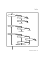
Granting Privileges
Granting Privileges
The authorization to use a database is called a privilege. For example, the
authorization to use a database is called the Connect privilege, and the authorization to insert a row into a table is called the Insert privilege. You control
the use of a database by granting these privileges to other users or by
revoking them.
Two groups of privileges control the actions a user can perform on data.
These include database-level privileges, which affect the entire database, and
table-level privileges, which relate to individual tables. In addition to these
two groups, procedure-level priviliges determine who can execute a
procedure.
Database-Level Privileges
The three levels of database privilege provide an overall means of controlling
who accesses a database.
Connect Privilege
The least of the privilege levels is Connect, which gives a user the basic ability
to query and modify tables. Users with the Connect privilege can perform the
following functions:
■
Execute the SELECT, INSERT, UPDATE, and DELETE statements,
provided that they have the necessary table-level privileges
■
Execute a stored procedure, provided that they have the necessary
table-level privileges
■
Create views, provided that they are permitted to query the tables on
which the views are based
■
Create temporary tables and create indexes on the temporary tables
Before users can access a database, they must have the Connect privilege.
Ordinarily, in a database that does not contain highly sensitive or private
data, you give the GRANT CONNECT TO PUBLIC privilege shortly after you
create the database.
10-6
Informix Guide to SQL: Tutorial
Database-Level Privileges
If you do not grant the Connect privilege to public, the only users who can
access the database through the database server are those to whom you
specifically grant the Connect privilege. If limited users should have access,
this privilege lets you provide it to them and deny it to all others.
The Users and the Public
Privileges are granted to single users by name or to all users under the name
of public. Any privileges granted to public serve as default privileges.
Prior to executing a statement, the database server determines whether a user
has the necessary privileges. (The information is in the system catalog; see
“Privileges in the System Catalog” on page 10-10.)
The database server looks first for privileges that are granted specifically to
the requesting user. If it finds such a grant, it uses that information. It then
checks to see if less restrictive privileges have been granted to public. If so,
the database server uses the less-restrictive privileges. If no grant has been
made to that user, the database server looks for privileges granted to public.
If it finds a relevant privilege, it uses that one.
Thus, to set a minimum level of privilege for all users, grant privileges to
public. You can override that, in specific cases, by granting higher individual
privileges to users.
Resource Privilege
The Resource privilege carries the same authorization as the Connect
privilege. In addition, users with the Resource privilege can create new,
permanent tables, indexes, and stored procedures, thus permanently
allocating disk space.
Granting and Limiting Access to Your Database
10-7
Ownership Rights
Database Administrator Privilege
The highest level of database privilege is Database Administrator, or DBA.
When you create a database, you are automatically the DBA. Holders of the
DBA privilege can perform the following functions:
■
Execute the DROP DATABASE, START DATABASE, and
ROLLFORWARD DATABASE statements
■
Drop or alter any object regardless of who owns it
■
Create tables, views, and indexes to be owned by other users
■
Grant database privileges, including the DBA privilege, to another
user
■
Alter the NEXT SIZE (but no other attribute) of the system catalog
tables, and insert, delete, or update rows of any system catalog table
except systables
Warning: Although users with the DBA privilege can modify most system catalog
tables, Informix strongly recommends that you do not update, delete, or insert any
rows in them. Modifying the system catalog tables can destroy the integrity of the
database. Informix does support using the ALTER TABLE statement to modify the size
of the next extent of system catalog tables.
Ownership Rights
The database, and every table, view, index, procedure, and synonym in it, has
an owner. The owner of an object is usually the person who created it,
although a user with the DBA privilege can create objects to be owned by
others.
The owner of an object has all rights to that object and can alter or drop it
without additional privileges.
10-8
Informix Guide to SQL: Tutorial
Table-Level Privileges
Table-Level Privileges
You can apply seven privileges, table by table, to allow nonowners the
privileges of owners. Four of them, the Select, Insert, Delete, and Update
privileges, control access to the contents of the table. The Index privilege
controls index creation. The Alter privilege controls the authorization to
change the table definition. The References privilege controls the
authorization to specify referential constraints on a table.
In an ANSI-compliant database, only the table owner has any privileges. In
other databases, the database server, as part of creating a table, automatically
grants all table privileges except Alter and References to public. Automatically granting all table privileges to public means that a newly created table
is accessible to any user with the Connect privilege. If this is not what you
want (if users exist with the Connect privilege who should not be able to
access this table), you must revoke all privileges on the table from public
after you create the table.
Access Privileges
Four privileges govern how users can access a table. As the owner of the
table, you can grant or withhold the following privileges independently:
■
The Select privilege allows selection, including selecting into
temporary tables.
■
The Insert privilege allows a user to add new rows.
■
The Update privilege allows a user to modify existing rows.
■
The Delete privilege allows a user to delete rows.
The Select privilege is necessary for a user to retrieve the contents of a table.
However, the Select privilege is not a precondition for the other privileges. A
user can have Insert or Update privileges without having the Select privilege.
For example, your application might have a usage table. Every time a certain
program is started, it inserts a row into the usage table to document that it
was used. Before the program terminates, it updates that row to show how
long it ran and perhaps to record counts of work its user performed.
If you want any user of the program to be able to insert and update rows in
this usage table, grant Insert and Update privileges on it to public. However,
you might grant the Select privilege to only a few users.
Granting and Limiting Access to Your Database
10-9
Table-Level Privileges
Privileges in the System Catalog
Privileges are recorded in the system catalog tables. Any user with the
Connect privilege can query the system catalog tables to determine what
privileges have been granted and to whom.
Database privileges are recorded in the sysusers table, in which the primary
key is user ID, and the only other column contains a single character C, R, or
D for the privilege level. A grant to the keyword of PUBLIC is reflected as a
user name of public (lowercase).
Table-level privileges are recorded in systabauth, which uses a composite
primary key of the table number, grantor, and grantee. In the tabauth
column, the privileges are encoded in the list that the following diagram
shows.
unconditional Update
Insert
Index
unconditional Select
su-idxar
* if column privilege granted
Figure 10-1
List of Encoded
Priviliges
References
Alter
Delete
A hyphen means an ungranted privilege, so that a grant of all privileges is
shown as su-idxar, and -u------ shows a grant of only Update. The code
letters are normally lowercase, but they are uppercase when the keywords
WITH GRANT OPTION are used in the GRANT statement.
When an asterisk (*) appears in the third position, some column-level
privilege exists for that table and grantee. The specific privilege is recorded
in syscolauth. Its primary key is a composite of the table number, the grantor,
the grantee, and the column number. The only attribute is a three-letter list
that shows the type of privilege: s, u, or r.
10-10
Informix Guide to SQL: Tutorial
Table-Level Privileges
Index, Alter, and References Privileges
The Index privilege permits its holder to create and alter indexes on the table.
The Index privilege, similar to the Select, Insert, Update, and Delete
privileges, is granted automatically to public when a table is created.
You can grant the Index privilege to anyone, but to exercise the ability, the
user must also hold the Resource database privilege. So, although the Index
privilege is granted automatically (except in ANSI-compliant databases),
users who have only the Connect privilege to the database cannot exercise
their Index privilege. Such a limitation is reasonable because an index can fill
a large amount of disk space.
The Alter privilege permits its holder to use the ALTER TABLE statement on
the table, including the power to add and drop columns, reset the starting
point for SERIAL columns, and so on. You should grant the Alter privilege
only to users who understand the data model very well and whom you trust
to exercise their power very carefully.
The References privilege allows you to impose referential constraints on a
table. As with the Alter privilege, you should grant the References privilege
only to users who understand the data model very well.
Column-Level Privileges
You can qualify the Select, Update, and References privileges with the names
of specific columns. Naming specific columns allows you to grant very
specific access to a table. You can permit a user to see only certain columns,
to update only certain columns, or to impose referential constraints on
certain columns.
Granting and Limiting Access to Your Database
10-11
Table-Level Privileges
Using INFORMIX-OnLine Dynamic Server (so that table data can be inspected
only through a call to the database server), this feature solves the problem
that only certain users should know the salary, performance review or other
sensitive attributes of an employee. To make the example specific, suppose a
table of employee data is defined as the following example shows:
CREATE TABLE hr_data
(
emp_key INTEGER,
emp_name CHAR(40),
hire_date DATE,
dept_num SMALLINT,
user-id CHAR(18),
salary DECIMAL(8,2)
performance_level CHAR(1),
performance_notes TEXT
)
Because this table contains sensitive data, you execute the following
statement immediately after you create it:
REVOKE ALL ON hr_data FROM PUBLIC
For selected persons in the Human Resources department and for all
managers, you execute the following statement:
GRANT SELECT ON hr_data TO harold_r
In this way, you permit certain users to view all columns. (The final section
of this chapter discusses a way to limit the view of managers to their
employees only.) For the first-line managers who carry out performance
reviews, you could execute a statement such as the following one:
GRANT UPDATE (performance_level, performance_notes)
ON hr_data TO wallace_s, margot_t
This statement permits the managers to enter their evaluations of their
employees. You would execute a statement such as the following one only for
the manager of the Human Resources department or whoever is trusted to
alter salary levels:
GRANT UPDATE (salary) ON hr_data to willard_b
For the clerks in the Human Resources department, you could execute a
statement such as the following one:
GRANT UPDATE (emp_key, emp_name, hire_date, dept_num)
ON hr_data TO marvin_t
10-12
Informix Guide to SQL: Tutorial
Procedure-Level Privileges
This statement gives certain users the ability to maintain the nonsensitive
columns but denies them authorization to change performance ratings or
salaries. The person in the MIS department who assigns computer user IDs is
the beneficiary of a statement such as the following one:
GRANT UPDATE (user_id) ON hr_data TO eudora_b
On behalf of all users who are allowed to connect to the database, but who
are not authorized to see salaries or performance reviews, execute statements
such as the following one to permit them to see the nonsensitive data:
GRANT SELECT (emp_key, emp_name, hire_date, dept_num, user-id)
ON hr_data TO george_b, john_s
These users can perform queries such as the following one:
SELECT COUNT(*) FROM hr_data WHERE dept_num IN (32,33,34)
However, any attempt to execute a query such as the following one produces
an error message and no data:
SELECT performance_level FROM hr_data
WHERE emp_name LIKE '*Smythe'
Procedure-Level Privileges
You can apply the Execute privilege on a procedure to authorize nonowners
to run a procedure. If you create a procedure in a database that is not ANSI
compliant, the default procedure-level privilege is PUBLIC; you do not need
to grant the Execute privilege to specific users unless you have first revoked
it. If you create a procedure in an ANSI-compliant database, no other users
have the Execute privilege by default; you must grant specific users the
Execute privilege. The following example grants the Execute privilege to the
user orion so that orion can use the stored procedure that is named
read-address:
GRANT EXECUTE ON read_address TO orion;
Procedure-level privileges are recorded in the sysprocauth system catalog
table. The sysprocauth table uses a primary key of the procedure number,
grantor, and grantee. In the procauth column, the execute privilege is
indicated by a lowercase letter e. If the execute privilege was granted with the
WITH GRANT option, the privilege is represented by an uppercase letter E.
Granting and Limiting Access to Your Database
10-13
Automating Privileges
For more information on procedure-level privileges, see “Privileges on
Stored Procedures” on page 12-15.
Automating Privileges
This design might seem to force you to execute a tedious number of GRANT
statements when you first set up the database. Furthermore, privileges
require constant maintenance as people change jobs. For example, if a clerk
in Human Resources is terminated, you want to revoke the Update privilege
as soon as possible; otherwise the unhappy employee might execute a
statement such as the following one:
UPDATE hr_data
SET (emp_name, hire_date, dept_num) = (NULL, NULL, 0)
Less dramatic, but equally necessary, changes of privilege are required daily,
or even hourly, in any model that contains sensitive data. If you anticipate
this need, you can prepare some automated tools to help maintain privileges.
Your first step should be to specify privilege classes that are based on the jobs
of the users, not on the structure of the tables. For example, a first-line
manager needs the following privileges:
■
The Select and limited Update privilege on the hypothetical hr_data
table
■
The Connect privilege to this and other databases
■
Some degree of privilege on several tables in those databases
When the manager is promoted to a staff position or sent to a field office, you
must revoke all those privileges and grant a new set of privileges.
Define the privilege classes you support, and for each class specify the
databases, tables, and columns to which you must give access. Then devise
two automated procedures for each class, one to grant the class to a user and
one to revoke it.
10-14
Informix Guide to SQL: Tutorial
Automating Privileges
Automating with INFORMIX-4GL
The mechanism you use depends on your operating system and other tools.
If you are a programmer, one of the tools you can use is INFORMIX-4GL. 4GL
makes it easy to program a simple user interaction, as the following example
shows:
DEFINE mgr_id char(20)
PROMPT 'What is the user-id of the new manager? ' FOR mgr_id
CALL table_grant ('SELECT', 'hr_data', mgr_id)
Unfortunately, although INFORMIX-4GL allows you to mix GRANT and
REVOKE statements freely with other program statements, it does not let you
create parameters from them from program variables. To customize a GRANT
statement with a user ID that is taken from user input, the program must
build the statement as a string, prepare it with a PREPARE statement, and
execute it with an EXECUTE statement. (These statements are discussed in
detail in Chapter 5, “Programming with SQL,” where the following example
is analyzed in detail.)
The following example shows one possible definition of the 4GL function
table_grant(), which is invoked by the CALL statement in the preceding
example:
FUNCTION table_grant (priv_to_grant, table_name, user_id)
DEFINE priv_to_grant char(100),{may include columnlist}
table_name CHAR(20),
user_id CHAR(20),
grant_stmt CHAR(200)
LET grant_stmt =' GRANT ', priv_to_grant,
' ON ', table_name,
' TO ', user_id
WHENEVER ERROR CONTINUE
PREPARE the_grant FROM grant_stmt
IF status = 0 THEN
EXECUTE the_grant
END IF
IF status <> 0 THEN
DISPLAY 'Sorry, got error #', status, 'attempting:'
DISPLAY '
', grant_stmt
END IF
WHENEVER ERROR STOP
END FUNCTION
Granting and Limiting Access to Your Database
10-15
Automating Privileges
Automating with a Command Script
Your operating system probably supports automatic execution of command
scripts. In most operating environments, interactive SQL tools such as
DB-Access and INFORMIX-SQL accept commands and SQL statements to
execute from the command line. You can combine these two features to
automate privilege maintenance.
The details depend on your operating system and the version of DB-Access
or INFORMIX-SQL that you are using. In essence, you want to create a
command script that performs the following functions:
■
Takes a user ID whose privileges are to be changed as its parameter
■
Prepares a file of GRANT or REVOKE statements customized to
contain that user ID
■
Invokes DB-Access or INFORMIX-SQL with parameters that tell it to
select the database and execute the prepared file of GRANT or
REVOKE statements
In this way, you can reduce the change of the privilege class of a user to one
or two commands.
Using Roles
Another way to avoid the difficulty of changing user privileges on a case by
case basis is to use roles. The concept of a role in the database environment is
similar to the group concept in an operating system. A role is a database
feature that lets the DBA standardize and change the privileges of many users
by treating them as members of a class.
For example, you can create a role called news_mes that grants connect, insert,
and delete privileges for the databases that handle company news and
messages. When a new employee arrives, you need only add that person to
the role news_mes. The new employee acquires the privileges of the role
news_mes. This process also works in reverse. To change the privileges of all
the members of news_mes, change the privileges of the role.
10-16
Informix Guide to SQL: Tutorial
Automating Privileges
Creating a Role
To start the role creation process, determine the name of the role along with
the connections and privileges you want to grant. Although the connections
and privileges are strictly in your domain, you need to consider some factors
when you name a role. Do not use any of the following words as role names.
alter
connect
DBA
default
delete
execute
index
insert
none
null
public
references
resource
select
update
A role name must be different from existing role names in the database. A
role name must also be different from user names that are known to the
operating system, including network users known to the server machine. To
make sure your role name is unique, check the names of the users in the
shared memory structure who are currently using the database as well as the
following system catalog tables:
■
sysusers
■
systabauth
■
syscolauth
■
sysprocauth
■
sysfragauth
■
sysroleauth
When the situation is reversed, and you are adding a user to the database,
check that the user name is not the same as any of the existing role names.
After you have approved the role name, use the CREATE ROLE statement to
create a new role. After the role is created, all privileges for role administration are, by default, given to the DBA.
Manipulating User Privileges and Granting Roles to Other Roles
As DBA, you can use the GRANT statement to grant role privileges to users.
You can also give a user the option to grant privileges to other users. Use the
WITH GRANT OPTION clause of the GRANT statement to do this. You can use
the WITH GRANT OPTION clause only when you are granting privileges to a
user.
Granting and Limiting Access to Your Database
10-17
Automating Privileges
For example, the following query returns an error because you are granting
privileges to a role with the grantable option:
GRANT SELECT on tab1 to rol1
WITH GRANT OPTION
Important: Do not use the WITH GRANT OPTION clause of the GRANT statement
when you grant privileges to a role. Only a user can grant privileges to other users.
When you grant role privileges, you can substitute a role name for the user
name in the GRANT statement. You can grant a role to another role. For
example, say that role A is granted to role B. When a user enables role B, the
user gets privileges from both role A and role B.
However, a cycle of role-grant cannot be transitive. If role A is granted role B,
and role B is granted role C, then granting C to A returns an error.
If you need to change privileges, use the REVOKE statement to delete the
existing privileges, and then use the GRANT statement to add the new
privileges.
Users Need to Enable Roles
After the DBA grants privileges and adds users to a role, you must use the SET
ROLE statement in a database session to enable the role. Unless you enable
the role, you are limited to the privileges that are associated with PUBLIC or
the privileges that are directly granted to you because you are the owner of
the object.
Confirming Membership In Roles and Dropping Roles
You can find yourself in a situation where you are uncertain which user is
included in a role. Perhaps you did not create the role or the person who
created the role is not available. Issue queries against the sysroleauth and
sysusers tables to find who is authorized for which table and how many roles
are in existence.
10-18
Informix Guide to SQL: Tutorial
Controlling Access to Data Using Stored Procedures
After you determine which users are members of which roles, you might
discover that some roles are no longer useful. To remove a role, use the DROP
ROLE statement. Before you remove a role, the following conditions must be
met:
■
Only roles that are listed in the sysusers catalog table as a role can be
destroyed.
■
You must have DBA privileges, or you must be given the grantable
option in the role to drop a role.
Controlling Access to Data Using Stored Procedures
You can use a stored procedure to control access to individual tables and
columns in the database. You can accomplish various degrees of access
control through a procedure. (Stored procedures are fully described in
Chapter 12, “Creating and Using Stored Procedures.”) A powerful feature of
Stored Procedure Language (SPL) is the ability to designate a stored
procedure as a DBA-privileged procedure. When you write a DBA-privileged
procedure, you can allow users who have few or no table privileges to have
DBA privileges when they execute the procedure. In the procedure, users can
carry out very specific tasks with their temporary DBA privilege. The DBAprivileged feature lets you accomplish the following tasks:
■
You can restrict how much information individual users can read
from a table.
■
You can restrict all the changes that are made to the database and
ensure that entire tables are not emptied or changed accidentally.
■
You can monitor an entire class of changes made to a table, such as
deletions or insertions.
■
You can restrict all object creation (data definition) to occur within a
stored procedure so that you have complete control over how tables,
indexes, and views are built.
Granting and Limiting Access to Your Database
10-19
Restricting Reads of Data
Restricting Reads of Data
The procedure in the following example hides the SQL syntax from users, but
it requires that users have the Select privilege on the customer table. If you
want to restrict what users can select, write your procedure to work in the
following environment:
■
You are the DBA of the database.
■
The users have the Connect privilege to the database. They do not
have the Select privilege on the table.
■
Your stored procedure (or set of stored procedures) is created using
the DBA keyword.
■
Your stored procedure (or set of stored procedures) reads from the
table for users.
If you want users to read only the name, address, and telephone number of a
customer, you can modify the procedure as the following example shows:
CREATE DBA PROCEDURE read_customer(cnum INT)
RETURNING CHAR(15), CHAR(15), CHAR(18);
DEFINE p_lname,p_fname CHAR(15);
DEFINE p_phone CHAR(18);
SELECT fname, lname, phone
INTO p_fname, p_lname, p_phone
FROM customer
WHERE customer_num = cnum;
RETURN p_fname, p_lname, p_phone;
END PROCEDURE;
10-20
Informix Guide to SQL: Tutorial
Restricting Changes to Data
Restricting Changes to Data
Using stored procedures, you can restrict changes made to a table. Simply
channel all changes through a stored procedure. The stored procedure makes
the changes, rather than users making the changes directly. If you want to
limit users to deleting one row at a time to ensure that they do not
accidentally remove all the rows in the table, set up the database with the
following privileges:
■
You are the DBA of the database.
■
All the users have the Connect privilege to the database. They might
have the Resource privilege. They do not have the Delete privilege
(for this example) on the table being protected.
■
Your stored procedure is created using the DBA keyword.
■
Your stored procedure performs the deletion.
Write a stored procedure similar to the following one, which deletes rows
from the customer table using a WHERE clause with the customer_num that
the user provides:
CREATE DBA PROCEDURE delete_customer(cnum INT)
DELETE FROM customer
WHERE customer_num = cnum;
END PROCEDURE;
Monitoring Changes to Data
Using stored procedures, you can create a record of changes made to a
database. You can record changes made by a particular user, or you can make
a record of each time a change is made.
Granting and Limiting Access to Your Database
10-21
Monitoring Changes to Data
You can monitor all the changes made to the database by a single user. Simply
channel all changes through stored procedures that keep track of changes
that each user makes. If you want to record each time the user acctclrk
modifies the database, set up the database with the following privileges:
■
You are the DBA of the database.
■
All other users have the Connect privilege to the database. They
might have the Resource privilege. They do not have the Delete
privilege (for this example) on the table being protected.
■
Your stored procedure is created using the DBA keyword.
■
Your stored procedure performs the deletion and records that a
certain user has made a change.
Write a stored procedure similar to the following one, which uses a customer
number the user provides to update a table. If the user happens to be acctclrk,
a record of the deletion is put in the file updates.
CREATE DBA PROCEDURE delete_customer(cnum INT)
DEFINE username CHAR(8);
DELETE FROM customer
WHERE customer_num = cnum;
IF username = 'acctclrk' THEN
SYSTEM 'echo Delete from customer by acctclrk >>
/mis/records/updates' ;
ENF IF
END PROCEDURE;
To monitor all the deletions made through the procedure, remove the IF
statement and make the SYSTEM statement more general. If you change the
previous procedure to record all deletions, it looks like the procedure shown
next.
CREATE DBA PROCEDURE delete_customer(cnum INT)
DEFINE username CHAR(8);
LET username = USER ;
DELETE FROM tbname WHERE customer_num = cnum;
SYSTEM
'echo Deletion made from customer table, by '||username
||'>>/hr/records/deletes';
END PROCEDURE;
10-22
Informix Guide to SQL: Tutorial
Restricting Object Creation
Restricting Object Creation
To put restraints on what objects are built and how they are built, use stored
procedures within the following setting:
■
You are the DBA of the database.
■
All the other users have the Connect privilege to the database. They
do not have the Resource privilege.
■
Your stored procedure (or set of stored procedures) is created using
the DBA keyword.
■
Your stored procedure (or set of stored procedures) creates tables,
indexes, and views in the way you defined them. You might use such
a procedure to set up a training database environment.
Your procedure might include the creation of one or more tables and
associated indexes, as the following example shows:
CREATE DBA PROCEDURE all_objects()
CREATE TABLE learn1 (intone SERIAL, inttwo INT NOT NULL,
charcol CHAR(10) );
CREATE INDEX learn_ix ON learn1 (inttwo);
CREATE TABLE toys (name CHAR(15) NOT NULL UNIQUE,
description CHAR(30), on_hand INT);
END PROCEDURE;
To use the all_objects procedure to control additions of columns to tables,
revoke the Resource privilege on the database from all users. When users try
to create a table, index, or view using an SQL statement outside your
procedure, they cannot do so. When users execute the procedure, they have
a temporary DBA privilege so the CREATE TABLE statement, for example,
succeeds, and you are guaranteed that every column that is added has a
constraint that is placed on it. In addition, objects that users create are owned
by that user. For the all_objects procedure, whoever executes the procedure
owns the two tables and the index.
Granting and Limiting Access to Your Database
10-23
Using Views
Using Views
A view is a synthetic table. You can query it as if it were a table, and in some
cases, you can update it as if it were a table. However, it is not a table. It is a
synthesis of the data that exists in real tables and other views.
The basis of a view is a SELECT statement. When you create a view, you define
a SELECT statement that generates the contents of the view at the time the
view is accessed. A user also queries a view using a SELECT statement. The
database server merges the SELECT statement of the user with the one
defined for the view and then actually performs the combined statements.
The result has the appearance of a table; it is similar enough to a table that a
view even can be based on other views, or on joins of tables and other views.
Because you write a SELECT statement that determines the contents of the
view, you can use views for any of the following purposes:
■
To restrict users to particular columns of tables
You name only permitted columns in the select list in the view.
■
To restrict users to particular rows of tables
You specify a WHERE clause that returns only permitted rows.
■
To constrain inserted and updated values to certain ranges
You can use the WITH CHECK OPTION (discussed on page 10-30) to
enforce constraints.
■
To provide access to derived data without having to store redundant
data in the database
You write the expressions that derive the data into the select list in
the view. Each time you query the view, the data is derived anew. The
derived data is always up to date, yet no redundancies are
introduced into the data model.
■
To hide the details of a complicated SELECT statement
You hide complexities of a multitable join in the view so that neither
users nor application programmers need to repeat them.
10-24
Informix Guide to SQL: Tutorial
Creating Views
Creating Views
The following example creates a view based on a table in the stores7
database:
CREATE VIEW name_only AS
SELECT customer_num, fname, lname FROM customer
The view exposes only three columns of the table. Because it contains no
WHERE clause, the view does not restrict the rows that can appear.
GLS
The following example creates a view based on a table that is available when
a locale other than the default U.S. English locale using the ISO8859-1 code set
has been enabled. In the example, the view, column, and table names contain
non-English characters.
CREATE VIEW çà_va AS
SELECT numéro, nom FROM abonnés;
♦
The following example is based on the join of two tables:
CREATE VIEW full_addr AS
SELECT address1, address2, city, state.sname, zipcode
FROM customer, state
WHERE customer.state = state.code
The table of state names reduces the redundancy of the database; it lets you
store the full state names only once, which can be useful for long state names
such as Minnesota. This full_addr view lets users retrieve the address as if
the full state name were stored in every row. The following two queries are
equivalent:
SELECT * FROM full_addr WHERE customer_num = 105
SELECT address1, address2, city, state.sname, zipcode
FROM customer, state
WHERE customer.state = state.code
AND customer_num = 105
However, be careful when you define views that are based on joins. Such
views are not modifiable; that is, you cannot use them with UPDATE, DELETE,
or INSERT statements. (Modifying through views is covered beginning on
page 10-28.)
The following example restricts the rows that can be seen in the view:
CREATE VIEW no_cal_cust AS
SELECT * FROM customer WHERE NOT state = 'CA'
Granting and Limiting Access to Your Database
10-25
Creating Views
This view exposes all columns of the customer table, but only certain rows.
The following example is a view that restricts users to rows that are relevant
to them:
CREATE VIEW my_calls AS
SELECT * FROM cust_calls WHERE user_id = USER
All the columns of the cust_calls table are available but only in those rows
that contain the user IDs of the users who can execute the query.
Duplicate Rows from Views
A view might produce duplicate rows, even when the underlying table has
only unique rows. If the view SELECT statement can return duplicate rows,
the view itself can appear to contain duplicate rows.
You can prevent this problem in two ways. One way is to specify DISTINCT
in the select list in the view. However, specifying DISTINCT makes it impossible to modify through the view. The alternative is to always select a column
or group of columns that is constrained to be unique. (You can be sure that
only unique rows are returned if you select the columns of a primary key or
of a candidate key. Primary and candidate keys are discussed in Chapter 8,
“Building Your Data Model.”)
Restrictions on Views
Because a view is not really a table, it cannot be indexed, and it cannot be the
object of such statements as ALTER TABLE and RENAME TABLE. The columns
of a view cannot be renamed with RENAME COLUMN. To change anything
about the definition of a view, you must drop the view and re-create it.
Because it must be merged with the user’s query, the SELECT statement on
which a view is based cannot contain any of the following clauses:
INTO TEMP
UNION
ORDER BY
10-26
Informix Guide to SQL: Tutorial
The user’s query might contain INTO TEMP; if the view also
contains it, the data would not know where to go.
The user’s query might contain UNION. No meaning has been
defined for nested UNION clauses.
The user’s query might contain ORDER BY. If the view also
contains it, the choice of columns or sort directions could be in
conflict.
Creating Views
When the Basis Changes
The tables and views on which a view is based can change in several ways.
The view automatically reflects most of the changes.
When a table or view is dropped, any views in the same database that depend
on it are automatically dropped.
The only way to alter the definition of a view is to drop and re-create it.
Therefore, if you change the definition of a view on which other views
depend, you must also re-create the other views (because they all have been
dropped).
When a table is renamed, any views in the same database that depend on it
are modified to use the new name. When a column is renamed, views in the
same database that depend on that table are updated to select the proper
column. However, the names of columns in the views themselves are not
changed. For an example of this, recall the following view on the customer
table:
CREATE VIEW name_only AS
SELECT customer_num, fname, lname FROM customer
Now suppose that the customer table is changed in the following way:
RENAME COLUMN customer.lname TO surname
To select last names of customers directly, you must now select the new
column name. However, the name of the column as seen through the view is
unchanged. The following two queries are equivalent:
SELECT fname, surname FROM customer
SELECT fname, lname FROM name_only
When you alter a table by dropping a column, views are not modified. If they
are used, error -217 (Column not found in any table in the query)
occurs. The reason views are not dropped is that you can change the order of
columns in a table by dropping a column and then adding a new column of
the same name. If you do this, views based on that table continue to work.
They retain their original sequence of columns.
INFORMIX-OnLine Dynamic Server permits you to base a view on tables and
views in external databases. Changes to tables and views in other databases
are not reflected in views. Such changes might not be apparent until someone
queries the view and gets an error because an external table changed.
Granting and Limiting Access to Your Database
10-27
Modifying Through a View
Modifying Through a View
You can modify views as if they were tables. Some views can be modified and
others not, depending on their SELECT statements. The restrictions are
different, depending on whether you use DELETE, UPDATE, or INSERT statements.
No modification is possible on a view when its SELECT statement contains
any of the following features:
■
A join of two or more tables
Many anomalies arise if the database server tries to distribute
modified data correctly across the joined tables.
■
An aggregate function or the GROUP BY clause
The rows of the view represent many combined rows of data; the
database server cannot distribute modified data into them.
■
The DISTINCT keyword or its synonym UNIQUE
The rows of the view represent a selection from among possibly
many duplicate rows; the database server cannot tell which of the
original rows should receive the modification.
When a view avoids all these things, each row of the view corresponds to
exactly one row of one table. Such a view is modifiable. (Of course, particular
users can modify a view only if they have suitable privileges. Privileges on
views are discussed beginning on page 10-31.)
Deleting Through a View
A modifiable view can be used with a DELETE statement as if it were a table.
The database server deletes the proper row of the underlying table.
Updating a View
You can use a modifiable view with an UPDATE statement as if it were a table.
However, a modifiable view can still contain derived columns; that is,
columns that are produced by expressions in the select list of the CREATE
VIEW statement. You cannot update derived columns (sometimes called
virtual columns).
10-28
Informix Guide to SQL: Tutorial
Modifying Through a View
When a column is derived from a simple arithmetic combination of a column
with a constant value (for example, order_date+30), the database server
can, in principle, figure out how to invert the expression (in this case, by
subtracting 30 from the update value) and perform the update. However,
much more complicated expressions are possible, most of which cannot
easily be inverted. Therefore, the database server does not support updating
any derived column.
The following example shows a modifiable view that contains a derived
column and an UPDATE statement that can be accepted against it:
CREATE VIEW call_response(user_id,received,resolved,duration
)AS
SELECT user_id,call_dtime,res_dtime, res_dtime
call_dtime
FROM cust_calls
WHERE user_id = USER
UPDATE call_response SET resolved = TODAY
WHERE resolved IS NULL
The duration column of the view cannot be updated because it represents an
expression (the database server cannot, even in principle, decide how to
distribute an update value between the two columns named in the
expression). But as long as no derived columns are named in the SET clause,
the update can be performed as if the view were a table.
A view can return duplicate rows even though the rows of the underlying
table are unique. You cannot distinguish one duplicate row from another. If
you update one of a set of duplicate rows (for example, by using a cursor to
update WHERE CURRENT), you cannot be sure which row in the underlying
table receives the update.
Inserting into a View
You can insert rows into a view provided that the view is modifiable and
contains no derived columns. The reason for the second restriction is that an
inserted row must provide values for all columns, and the database server
cannot tell how to distribute an inserted value through an expression. An
attempt to insert into the call_response view, as the previous example shows,
would fail.
Granting and Limiting Access to Your Database
10-29
Modifying Through a View
When a modifiable view contains no derived columns, you can insert into it
as if it were a table. However, the database server uses null as the value for
any column that is not exposed by the view. If such a column does not allow
nulls, an error occurs, and the insert fails.
Using WITH CHECK OPTION
You can insert into a view a row that does not satisfy the conditions of the
view; that is, a row that is not visible through the view. You can also update
a row of a view so that it no longer satisfies the conditions of the view.
To avoid updating a row of a view so that it no longer satisfies the conditions
of the view, you can add the clause WITH CHECK OPTION when you create
the view. This clause asks the database server to test every inserted or
updated row to ensure that it meets the conditions set by the WHERE clause
of the view. The database server rejects the operation with an error if the
conditions are not met.
In the previous example, the view named call_response is defined as the
following example shows:
CREATE VIEW call_response(user_id,received,resolved,duration)AS
SELECT user_id,call_dtime,res_dtime,res_dtime -call_dtime
FROM cust_calls
WHERE user_id = USER
You can update the user_id column of the view, as the following example
shows:
UPDATE call_response SET user_id = 'lenora'
WHERE received BETWEEN TODAY AND TODAY-7
The view requires rows in which user_id equals USER. If a user named tony
performs this update, the updated rows vanish from the view. However, you
can create the view as the following example shows:
CREATE VIEW call_response (user_id,received,resolved,duration) AS
SELECT user_id,call_dtime,res_dtime,res_dtime-call_dtime
FROM cust_calls
WHERE user_id = USER
WITH CHECK OPTION
The preceding update by tony is rejected as an error.
10-30
Informix Guide to SQL: Tutorial
Privileges and Views
You can use the WITH CHECK OPTION feature to enforce any kind of data
constraint that can be stated as a Boolean expression. In the following
example, you can create a view of a table in which all the logical constraints
on data are expressed as conditions of the WHERE clause. Then you can
require all modifications to the table to be made through the view.
CREATE VIEW order_insert AS
SELECT * FROM orders O
WHERE order_date = TODAY -- no back-dated entries
AND EXISTS -- ensure valid foreign key
(SELECT * FROM customer C
WHERE O.customer_num = C.customer_num)
AND ship_weight < 1000 -- reasonableness checks
AND ship_charge < 1000
WITH CHECK OPTION
Because of EXISTS and other tests, which are expected to be successful when
retrieving existing rows, this view displays data from orders inefficiently.
However, if insertions to orders are made only through this view (and you
are not already using integrity constraints to constrain data), users cannot
insert a back-dated order, an invalid customer number, or an excessive
shipping weight and shipping charge.
Privileges and Views
When you create a view, the database server tests your privileges on the
underlying tables and views. When you use a view, only your privileges with
regard to the view are tested.
Privileges When Creating a View
Therefore, the database server tests to make sure that you have all the privileges that you need to execute the SELECT statement in the view definition. If
you do not, the view is not created.
This test ensures that users cannot gain unauthorized access to a table by
creating a view on the table and querying the view.
After you create the view, the database server grants you, the creator and
owner of the view, at least the Select privilege on it. No automatic grant is
made to public, as is the case with a newly created table.
Granting and Limiting Access to Your Database
10-31
Privileges When Using a View
The database server tests the view definition to see if the view is modifiable.
If it is, the database server grants you the Insert, Delete, and Update privileges on the view, provided that you also have those privileges on the
underlying table or view. In other words, if the new view is modifiable, the
database server copies your Insert, Delete, and Update privileges from the
underlying table or view, and grants them on the new view. If you have only
the Insert privilege on the underlying table, you receive only the Insert
privilege on the view.
This test ensures that users cannot use a view to gain access to any privileges
that they did not already have.
Because you cannot alter or index a view, the Alter and Index privileges are
never granted on a view.
Privileges When Using a View
When you attempt to use a view, the database server tests only the privileges
that you are granted on the view. It does not test your right to access the
underlying tables.
If you created the view, your privileges are the ones noted in the preceding
paragraph. If you are not the creator, you have the privileges that were
granted to you by the creator or someone who had the WITH GRANT OPTION
privilege.
Therefore you can create a table and revoke public access to it; then you can
grant limited access privileges to the table through views. The process of
creating such a table can be demonstrated through the previous examples
using the hr_data table. The following table shows its definition:
CREATE TABLE hr_data
(
emp_key INTEGER,
emp_name CHAR(40),
hire_date DATE,
dept_num SMALLINT,
user-id CHAR(18),
salary DECIMAL(8,2),
performance_level CHAR(1),
performance_notes TEXT
)
10-32
Informix Guide to SQL: Tutorial
Privileges When Using a View
The previous example centers on granting privileges directly on this table.
The following examples take a different approach. Assume that when the
table was created, the following statement was executed:
REVOKE ALL ON hr_data FROM PUBLIC
(Such a statement is not necessary in an ANSI-compliant database.) Now you
create a series of views for different classes of users. For those who should
have read-only access to the nonsensitive columns, you create the following
view:
CREATE VIEW hr_public AS
SELECT emp_key, emp_name, hire_date, dept_num, user_id
FROM hr_data
Users who are given the Select privilege for this view can see nonsensitive
data and update nothing. For Human Resources personnel who must enter
new rows, you create a different view, as the following example shows:
CREATE VIEW hr_enter AS
SELECT emp_key, emp_name, hire_date, dept_num
FROM hr_data
You grant these users both Select and Insert privileges on this view. Because
you, the creator of both the table and the view, have the Insert privilege on
the table and the view, you can grant the Insert privilege on the view to others
who have no privileges on the table.
On behalf of the person in the MIS department who enters or updates new
user IDs, you create still another view, as the following example shows:
CREATE VIEW hr_MIS AS
SELECT emp_key, emp_name, user_id
FROM hr_data
This view differs from the previous view in that it does not expose the
department number and date of hire.
Granting and Limiting Access to Your Database
10-33
Summary
Finally, the managers need access to all columns and they need the ability to
update the performance-review data for their own employees only. These
requirements can be met by creating a table, hr_data, that contains a
department number and a computer user IDs for each employee. Let it be a
rule that the managers are members of the departments that they manage.
Then the following view restricts managers to rows that reflect only their
employees:
CREATE VIEW hr_mgr_data AS
SELECT * FROM hr_data
WHERE dept_num =
(SELECT dept_num FROM hr_data
WHERE user_id = USER)
AND NOT user_id = USER
The final condition is required so that the managers do not have update
access to their own row of the table. Therefore, you can safely grant the
Update privilege to managers for this view, but only on selected columns, as
the following statement shows:
GRANT SELECT, UPDATE (performance_level, performance_notes)
ON hr_mgr_data TO peter_m
Summary
When a database contains public material, or when only you and trusted
associates use the database, security is not an important consideration, and
few of the ideas in this chapter are needed. But as more people are allowed
to use and modify the data, and as the data becomes increasingly confidential, you must spend more time and be ever more ingenious at controlling
the way users can approach the data.
10-34
Informix Guide to SQL: Tutorial
Summary
The techniques discussed here can be divided into the following groups:
■
Keeping data confidential
When the database resides in operating-system files, you can use
features of the operating system to deny access to the database. In
any case, you control the granting of the Connect privilege to keep
people out of the database.
When different classes of users have different degrees of authorization, you must give them all the Connect privilege. You can use
table-level privileges to deny access to confidential tables or
columns. Or, you can use a stored procedure to provide limited
access to confidential tables or columns. In addition, you can deny all
access to tables and allow it only through views that do not expose
confidential rows or columns.
■
Controlling changes to data and database structure
To safeguard the integrity of the data model, restrict grants of the
Resource, Alter, References, and DBA privileges. To ensure that only
authorized persons modify the data, control the grants of the Delete
and Update privileges and grant the Update privilege on as few
columns as possible. To ensure that consistent, reasonable data is
entered, grant the Insert privilege only on views that express logical
constraints on the data. Alternatively, to control the insertion and
modification of data, or the modification of the database itself, limit
access to constrictive stored procedures.
Granting and Limiting Access to Your Database
10-35
Chapter
Understanding Informix
Networking
What Is a Network?
.
.
.
.
.
.
.
.
.
.
.
.
.
11
.
.
.
.
.
11-4
Database Management System Configurations . . . . . . . . .
A Single-User Configuration . . . . . . . . . . . . . .
Advantages and Disadvantages of a Single-User System . . .
A Local Multiuser Configuration. . . . . . . . . . . . .
Advantages and Disadvantages of Local Multiuser Systems . .
A Remote Configuration . . . . . . . . . . . . . . .
Advantages and Disadvantages of Remote Network Connections
Single-Computer Configuration That Uses Network Communication
Advantages and Disadvantages of Local Loopback . . . . .
Distributed Databases . . . . . . . . . . . . . . . .
Advantages and Disadvantages of Distributed Databases . . .
Distributed Databases That Use Multiple Vendor Servers . . . .
11-4
11-5
11-6
11-7
11-8
11-9
11-10
11-10
11-11
11-12
11-12
11-13
Connecting to Data on a UNIX Network .
Example of Client/Server Connections
Environment Variables . . . . . .
Connection Information . . . . . .
SQL Connection Statements . . . .
.
.
.
.
.
.
.
.
.
.
.
.
.
.
.
.
.
.
.
.
.
.
.
.
.
.
.
.
.
.
.
.
.
.
.
.
.
.
.
.
.
.
.
.
.
.
.
.
.
.
11-14
11-15
11-16
11-17
11-17
Accessing Tables. . . . . . . . .
Using Synonyms with Table Names.
Synonym Chains . . . . . . .
.
.
.
.
.
.
.
.
.
.
.
.
.
.
.
.
.
.
.
.
.
.
.
.
.
.
.
.
.
.
11-18
11-19
11-20
Protecting Your Data in a Networked Environment . . . . . . .
Data Protection with INFORMIX-SE . . . . . . . . . . .
Data Protection with INFORMIX-OnLine Dynamic Server . . . .
Data Replication . . . . . . . . . . . . . . . . .
Backups . . . . . . . . . . . . . . . . . . . .
11-21
11-21
11-21
11-21
11-22
.
.
.
Data Integrity for Distributed Data .
Two-Phase Commit . . . . .
Summary .
11-2
.
.
Informix Guide to SQL: Tutorial
.
.
.
.
.
.
.
.
.
.
.
.
.
.
.
.
.
.
.
.
.
.
.
.
.
.
.
.
. 11-22
. 11-23
.
.
.
.
.
.
.
.
.
.
. 11-23
T
his chapter gives an overview of the use of databases on a computer
network. It introduces some commonly used terminology and illustrates
various network configurations. The chapter also presents an overview of
how the components of either a local or network connection fit together so
that a client application can find data on a database server.
This chapter discusses the following networking configurations that you can
use with Informix databases and points out some of their effects on
performance and usability:
■
All on one computer
■
A simple network connection
■
Multiple connections on a network
■
Data managed by non-Informix database servers
(INFORMIX-TP/XA)
You cannot simply build a computer network; you have to re-examine how
your applications and database servers share data. This chapter also covers
the following topics concerned with managing data that is shared over a
network:
■
Distributed data
■
Connecting to data
■
Protecting your data
■
Synonym chains
■
Network transparency
The final sections of the chapter discuss protecting your data in a networked
environment.
Understanding Informix Networking 11-3
What Is a Network?
What Is a Network?
A computer network is a group of computers, workstations, and other devices
connected together over a communications system to share resources and
data. A network site is simply the location of one of the computers on the
network. Sometimes the network sites are widely separated, but they might
also be in the same room or building. Two network sites can even coexist on
the same computer.
To make a practical computer network work, you must master a multitude of
technical details regarding hardware and software. Far too many details
exist, and they change too rapidly to cover them in this book. This chapter
provides a conceptual discussion of some of the issues that you might
encounter when you use a computer network. For more information, refer to
the manual that accompanies the Informix client/server product that you use
and to the manuals provided by the vendor of your operating system.
Database Management System Configurations
A relational database management system (RDBMS) includes all the components
necessary to create and maintain a relational database. An Informix RDBMS
has several pieces: the user interface, the database server, and the data itself.
It is easiest to think of these pieces as all being located in the same computer,
but many other arrangements are possible. In some arrangements, the application and the database server are on different computers, and the data is
distributed across several others.
The client applications of an RDBMS do not need to be modified to run on a
network. The communications tools that are part of all Informix products
handle the tasks of locating and attaching to the database servers. To the
application, a database on a networked computer appears no different than
a database on the computer where the application resides.
11-4
Informix Guide to SQL: Tutorial
A Single-User Configuration
A Single-User Configuration
Figure 11-1 shows a diagram of a simple database management system on a
single computer. The organization in Figure 11-1 is one you would typically
find on a personal computer that runs DOS. It is unusual to have a single-user
situation on a UNIX system, but you certainly can. One example of a singleuser UNIX system would be a desktop workstation in a development
environment.
personal computer
Figure 11-1
A Database
Management
System on a
Personal Computer
connection
INFORMIX-SE
User
Application
Databases
Understanding Informix Networking 11-5
A Single-User Configuration
The components of the system in Figure 11-1 are described in the following
list:
■
An application program. Any program that issues a query can be the
application. It could, for example, be a program written in
INFORMIX-4GL, a C language program with embedded SQL, or
compiled screen forms and reports.
■
A connection. On a simple system such as this one, the communication component is frequently so well integrated with the system
that it is omitted from diagrams and not discussed. However, it does
exist.
■
A database server. The database server receives queries from the
application, searches the database, and returns information to the
application. The database server manages or administers the
databases that it controls.
The database server in Figure 11-1 is a local server because it resides
on the same host computer as the client application.
■
A database. Databases are usually stored on a magnetic disk. If this
system were a UNIX system with INFORMIX-OnLine Dynamic Server,
the database might be located on some other medium, such as a
WORM (write-once read-many-times) drive controlled by
INFORMIX-OnLine/Optical.
Advantages and Disadvantages of a Single-User System
A configuration that involves only one computer is the easiest configuration
to set up and maintain, and it gives the fastest access to data. However, the
data is not available to users on other computers, and the size of the
databases or the amount of processing that is needed might outgrow the
capacity of the computer.
11-6
Informix Guide to SQL: Tutorial
A Local Multiuser Configuration
A Local Multiuser Configuration
Figure 11-2 shows another database management system configuration, a
multiuser system with a local database server such as one you might find on
a computer with a UNIX operating system.
Figure 11-2
A Database
Management
System on a UNIX
Computer
UNIX Computers
User
Application
Databases
Connection
User
Application
Database Server
The components of the systems in Figure 11-2 are similar to the components
in Figure 11-1 on page 11-5, as the following list describes:
■
Application programs. Two or more applications use the same
database server to access information in the databases. You might
have two users at individual terminals, as shown, or you might have
multiple windows on a single workstation.
Understanding Informix Networking 11-7
A Local Multiuser Configuration
■
A connection. On a local UNIX system, the following types of
connection are possible:
❑
Network connection
❑
Interprocess communication (IPC)
IPC is a UNIX feature that transfers information very quickly
between the application and the database server. It is available
only when the application and the database server reside on the
same computer. INFORMIX-SE databases use a type of IPC
connection that is called unnamed pipes and INFORMIX-OnLine
Dynamic Server databases use an IPC connection technique that
is called shared memory.
■
A database server. This database server will be either
INFORMIX-OnLine Dynamic Server or INFORMIX-SE.
■
Databases.
Advantages and Disadvantages of Local Multiuser Systems
A configuration that allows multiple users gives better access to the data than
does a single-user system. With a local database, a multiuser configuration is
still easy to set up and maintain. However, as with the single-user system, the
data is not available to users on other computers, and the size of the
databases or the amount of processing needed might outgrow the capacity of
the computer.
IPC shared memory provides very fast communication between the client
application and the database server. However, IPC shared memory
communication is vulnerable to programming errors if the client application
does explicit memory addressing or overindexes data arrays. Such errors do
not affect the application if you use IPC unnamed pipes or network
communication. (See “Single-Computer Configuration That Uses Network
Communication” on page 11-10.)
11-8
Informix Guide to SQL: Tutorial
A Remote Configuration
A Remote Configuration
Figure 11-3 shows a remote or network configuration, where the application
resides on one computer and the database server and its associated databases
reside on another computer on the network. In contrast, the database servers
in Figure 11-1 and Figure 11-2 are local database servers.
Figure 11-3
A Simple Network Connection
Host 1
Host 2
User
Application
Databases
Network connection
Database server
User
Application
In Figure 11-3, the applications might be INFORMIX-ESQL/COBOL or
INFORMIX-ESQL/C applications. The database server might be
INFORMIX-OnLine Dynamic Server (UNIX) or INFORMIX-SE for Windows NT.
Different computers are referred to as sites or host computers. The database
server in Figure 11-3 is a remote database server because it is on a different
host computer from the application that uses its services. A database server
can be local with respect to one application and remote with respect to
another application, as illustrated in Figure 11-6 on page 11-15.
Understanding Informix Networking 11-9
Single-Computer Configuration That Uses Network Communication
Advantages and Disadvantages of Remote Network Connections
The configuration shown in Figure 11-3 is an example of distributed processing.
In distributed processing, multiple computers contribute to a single
computing task. In this example, host1 handles the computing requirements
of the application, such as screen display, generation of reports, and printing;
host2 handles the computing required to manipulate information in the
databases. Using a network also gives the client application the opportunity
to access data from several computers.
Response from a database server using network communication is not as fast
as response from a database server using IPC because of the extra computing
required to prepare the data for network communication and because of the
transmit time. A network is somewhat more difficult to configure and
maintain than a local system that uses IPC communication.
Single-Computer Configuration That Uses Network
Communication
Figure 11-4 shows a configuration that behaves as if multiple sites were
residing on one computer. In this configuration, which is known as local
loopback, all the components are on the same computer, but the connections
are made as if they were connected through a network.
Because the connections use network software, the database server appears
to the application as a remote site. The dashed line indicates the division
between the two sites. The database administrator configures the system to
provide local or local loopback connections (or both).
11-10
Informix Guide to SQL: Tutorial
Single-Computer Configuration That Uses Network Communication
The software for the client application and the software for the database
server can be stored in the same directory, or the software can be stored in
two separate directories.
Figure 11-4
An Example of Local
Loopback
Computer
Client site
User
Server site
Application
Databases
Database server
Network
connection
Advantages and Disadvantages of Local Loopback
Local loopback allows you to test network operations without requiring an
actual remote computer, but it is not as fast as a IPC. However, unlike IPC
shared-memory communication, local loopback is not vulnerable to
corruption due to memory-addressing errors or overindexed data arrays.
(See “Advantages and Disadvantages of Local Multiuser Systems” on
page 11-8.)
Understanding Informix Networking 11-11
Distributed Databases
Distributed Databases
Although a network lets you separate the application from the data, the
application still is limited to the contents of a single database. With most
database servers, you can query or modify tables only in the current
database.
A distributed database has information on multiple databases that are
organized to appear as a single database to the user. The data can be
maintained by a variety of database servers and located on computers
supported by different operating systems and communication networks.
The OnLine database server allows you to query data in multiple databases
anywhere on the network. When the INFORMIX-TP/XA feature is added to
INFORMIX-OnLine Dynamic Server, you can create global transactions that
span multiple computer systems and even multiple XA-compliant database
systems from different vendors. INFORMIX-SE does not provide distributed
database processing capabilities.
INFORMIX-Gateway with DRDA allows you to perform distributed queries
that include non-Informix databases that conform to the distributed
relational database architecture (DRDA) protocols defined by IBM.
Advantages and Disadvantages of Distributed Databases
Distributed databases are useful because operations that use databases are
often naturally distributed into separate pieces, either organizationally,
geographically, or both. A distributed database system provides the
following advantages:
■
Local data can be kept locally where it is most easily maintained and
most frequently used.
■
Data from remote sites is available to all users.
■
Duplicate copies can be maintained for safety of the data.
A distributed database system has the following disadvantages:
11-12
■
Management of the distributed system is more involved than
management of a single-host system.
■
Network access is slower than local access.
Informix Guide to SQL: Tutorial
Distributed Databases That Use Multiple Vendor Servers
Distributed Databases That Use Multiple Vendor Servers
INFORMIX-TP/XA allows you to use database management systems from
multiple vendors to store and access your data. INFORMIX-TP/XA is a library
of functions that allows the INFORMIX-OnLine Dynamic Server database
server to act as a resource manager in a distributed transaction-processing
(DTP) environment that follows an interface standard, which was defined by
the X/Open Company.
The XA standard uses terminology that is different from the terminology
Informix products and documentation use. A transaction manager acts as an
intermediary and relays requests from a user interface to a resource manager.
Transaction managers are third-party products such as TUXEDO. In this
context, a resource manager corresponds to a database server. Figure 11-5
illustrates a configuration that uses transaction processing.
Figure 11-5
A Configuration That Uses a Transaction Manager
User
Transaction manager
Interface
INFORMIX
OnLine/XA
Vendor A
OnLine/XA
User
Interface
Vendor B
OnLine/XA
Client portion
of each
application
Server portion
of each
application
Resource
manager
Databases
Understanding Informix Networking 11-13
Connecting to Data on a UNIX Network
Connecting to Data on a UNIX Network
When the application and data are moved to separate computers, two
questions immediately arise. What connections can you implement? How do
you instruct your applications to find the data that is now somewhere else?
In fact, connecting a client application to a database server that is on a
networked computer is no different from connecting to a local database
server. To connect a client application with a database, you must consider the
following parts of your configuration:
■
Environment variables
■
Connection information
■
Connection statements
This section summarizes how connections are made for Version 6.0 and later
clients and servers. Detailed instructions for setting up local and network
connections, as well as for those between Version 6.0 servers and earlier
clients are given in the INFORMIX-OnLine Dynamic Server Administrator’s
Guide, the INFORMIX-SE Administrator’s Guide, and the INFORMIX-Gateway
with DRDA User Manual.
11-14
Informix Guide to SQL: Tutorial
Example of Client/Server Connections
Example of Client/Server Connections
Figure 11-6 shows local and networked connections of Version 6.0 and later
products. Although all these connections are possible, you cannot do them all
at once. Client X can make connection 1, 2, or 3, and Client Y can make
connection 4 or 5.
Host 1
Figure 11-6
Local and Network
Connection of
Version 6.0 and
Later Products
Host 2
A
B
OnLine 7.1
OnLine 7.1
7.1 Client Y
4
2
Daemon
1
5
sqlexecd
SE 7.1
7.1 Client X
3
To connect clients directly to OnLine database servers, use either shared
memory (IPC) or a network communications. OnLine database servers
(OnLine A and OnLine B in Figure 11-6) can communicate with each other.
Local clients can connect directly to an INFORMIX-SE database server using
unnamed pipes (IPC). Clients that are using network communications
connect to INFORMIX-SE by connecting first to a daemon, sqlexecd. A daemon
is a background process that listens for requests from other programs. The
system administrator starts the sqlexecd daemon. When a client requests a
connection to an INFORMIX-SE database server, sqlexecd notices the request
and creates a temporary (light gray arrows) connection between the client
and SE. This temporary connection (shown as (3) - (1) in Figure 11-6) enables
the client and INFORMIX-SE database server to establish a direct connection
(3). Then sqlexecd removes itself from the loop and leaves the client attached
to the SE database server.
Understanding Informix Networking 11-15
Environment Variables
Environment Variables
The Informix administrator must make sure that each user sets the correct
environment variables. The following list shows the most important
environment variables used by OnLine and INFORMIX-SE:
■
PATH
■
INFORMIXDIR
■
INFORMIXSERVER
■
TERM
■
DBPATH
■
ONCONFIG
The INFORMIXDIR environment variable must be set to the full pathname of
the directory where the Informix files reside. The PATH environment variable
must include the full pathname of the directory where the executables for
INFORMIX-SE and/or INFORMIX-OnLine Dynamic Server reside. These two
environment variables are required. After the Informix administrator has
specified them, you usually do not change them.
The INFORMIXSERVER environment variable is the name of the default
database server. It is also a required variable. You can choose to change
INFORMIXSERVER when you change applications.
The TERM (or TERMCAP and/or INFORMIXTERM) environment variable
enables the clients to recognize and communicate with your terminal. These
variables are system- and terminal-dependent. To set them, you might need
the assistance of your system administrator.
The DBPATH environment variable is optional. If the application does not
fully specify the location of an SE database server, the database server
searches the directories listed in DBPATH to find the specified database. Both
INFORMIX-OnLine Dynamic Server and INFORMIX-SE use the DBPATH
environment variable to specify directory names for reports, forms, and
command files.
When OnLine is initialized, it requires the ONCONFIG environment variable.
The ONCONFIG environment variable is not used by SE.
These environment variables are described in detail in Chapter 4 of the
Informix Guide to SQL: Reference.
11-16
Informix Guide to SQL: Tutorial
Connection Information
Connection Information
The $INFORMIXDIR/etc/sqlhosts file specifies the location of the database
server and the type of connection (protocol) for the database server. Each
database server that might be accessed by an application must have an entry
in sqlhosts file on every computer on the network.
In addition to the sqlhosts files, TCP/IP connections require entries in the
UNIX systems files, /etc/hosts and /etc/services. IPX/SPX connections also
require auxiliary files, However, unlike TCP/IP, the names of the auxiliary
files depend on the hardware vendor.
Informix database servers follow UNIX security requirements for making
connections. Thus, the UNIX system administrator might need to make
modifications to the /etc/passwd, /etc/hosts, rhosts and other related files.
These files are described in the INFORMIX-OnLine Dynamic Server Administrator’s Guide, the INFORMIX-SE Administrator’s Guide, the
INFORMIX-Gateway with DRDA User Manual, and operating-system manuals.
SQL Connection Statements
Before it can do anything else, the client application must execute a
CONNECT statement or a DATABASE statement to open a database. The
CONNECT statement is preferred because it conforms with both ANSI and
X/Open standards, which attempt to specify uniform syntax for networked
and nonnetworked environments.
The following command is an example of the CONNECT statement:
CONNECT TO databasename@servername
The application connects to the default database server that the
INFORMIXSERVER environment variable specifies if servername is omitted
from the previous statement.
If databasename is omitted, the application connects to the database server
servername but does not open a database. Before you can use a database, you
must issue a DATABASE, CREATE DATABASE, or START DATABASE statement.
The CONNECT statement does not give any information about the location of
the database server. The location information for the database server is in the
sqlhosts file. (Refer to “Connection Information” above.)
Understanding Informix Networking 11-17
Accessing Tables
You can also use the DISCONNECT statement to terminate the connection
between your application and the database server. To reestablish an active
connection and make it current, use the SET CONNECTION statement. You
can also use the DORMANT clause of the SET CONNECTION statement to
make the current connection dormant. Using the DORMANT clause of the SET
CONNECTION statement is particularly useful when you are working on a
multithreaded application. For more information regarding multithreaded
applications, see Chapter 11 of the INFORMIX-ESQL/C Programmer’s Manual.
The complete syntax for the CONNECT, DATABASE, DISCONNECT, and SET
CONNECTION statements is covered in Chapter 1 of the Informix Guide to
SQL: Syntax.
Accessing Tables
The database that a CONNECT, DATABASE or CREATE DATABASE statement
opens is the current database. If you are using INFORMIX-OnLine Dynamic
Server, you can query tables that are not in the current database. To refer to a
table in a database other than the current database, include the database
name as part of the table name, as illustrated in the following SELECT
statement:
SELECT name, number FROM salesdb:contacts
The database is salesdb. The table in salesdb is named contacts. You can use
the same notation in a join. When you must specify the database name
explicitly, the long table names can become cumbersome unless you use
aliases to shorten them, as the following example shows:
SELECT C.custname, S.phone
FROM salesdb:contacts C, stores:customer S
WHERE C.custname = S.company
You must qualify the database name with a database server name to specify a
table in a database that a different OnLine database server manages. For
example, the following SELECT statement refers to table customer from
database masterdb, which resides on the database server central:
SELECT O.order_num, C.fname, C.lname
FROM masterdb@central:customer C, sales@boston:orders O
WHERE C.customer_num = O.Customer_num
INTO TEMP mycopy
11-18
Informix Guide to SQL: Tutorial
Using Synonyms with Table Names
In the example, two tables are being joined. The joined rows are stored in a
temporary table mycopy in the current database. The tables are located in
two database servers, central and boston.
Informix allows you to overqualify (to give more information than is required)
table names. Because both table names are fully qualified, you cannot tell
whether the current database is masterdb or sales.
Using Synonyms with Table Names
A synonym is a name that you can use in place of another name. The main use
of the CREATE SYNONYM statement is to make it more convenient to refer to
tables that are not in the current database.
The preceding example has been revised as follows, to use synonyms for the
table names:
CREATE SYNONYM mcust FOR masterdb@central:customer;
CREATE SYNONYM bords FOR sales@boston:orders;
SELECT bords.order_num, mcust.fname, mcust.lname
FROM mcust, bords
WHERE mcust.customer_num = bords.Customer_num
INTO TEMP mycopy;
The CREATE SYNONYM statement stores the synonym name in the system
catalog table syssyntable in the current database. The synonym is available
to any query made within that database.
A short synonym makes it easier to write queries, but synonyms can play
another role. They allow you to move a table to a different database, or even
to a different computer, while leaving your queries the same.
Suppose you have several queries that refer to the tables customer and
orders. The queries are embedded in programs, forms, and reports. The
tables are part of database stores7, which is kept on database server avignon.
Now the decision is made that the same programs, forms, and reports are to
be made available to users of a different computer on the network (database
server nantes). Those users have a database that contains a table named
orders containing the orders at their location, but they need access to the
table customer at avignon.
Understanding Informix Networking 11-19
Synonym Chains
To those users, the customer table is external. Does this mean you must
prepare special versions of the programs and reports, versions in which the
customer table is qualified with a database server name? A better solution is
to create a synonym in the users’ database, as the following example shows:
DATABASE stores7@nantes;
CREATE SYNONYM customer FOR stores7@avignon:customer;
When the stored queries are executed in your database, the name customer
refers to the actual table. When they are executed in the other database, the
name is translated through the synonym into a reference to the external table.
Synonym Chains
To continue the preceding example, suppose that a new computer is added
to your network. Its name is db_crunch. The customer table and other tables
are moved to it to reduce the load on avignon. You can reproduce the table
on the new database server easily enough, but how can you redirect all
accesses to it? One way is to install a synonym to replace the old table, as the
following example shows:
DATABASE stores7@avignon EXCLUSIVE;
RENAME TABLE customer TO old_cust;
CREATE SYNONYM customer FOR stores7@db_crunch:customer;
CLOSE DATABASE;
When you execute a query within stores7@avignon, a reference to table
customer finds the synonym and is redirected to the version on the new
computer. Such redirection also happens for queries that are executed from
database server nantes. The synonym in the database stores7@nantes still
redirects references to customer to database stores7@avignon; however, the
new synonym there sends the query to database stores7@db_crunch.
Chains of synonyms can be useful when, as in this example, you want to
redirect all access to a table in one operation. However, you should update all
users’ databases as soon as possible so their synonyms point directly to the
table. You incur extra overhead in handling the extra synonyms, and the table
cannot be found if any computer in the chain is down.
11-20
Informix Guide to SQL: Tutorial
Protecting Your Data in a Networked Environment
You can run an application against a local database and later run the identical
application against a database on another computer. The program runs
equally well in either case (although it can run more slowly on the network
database). As long as the data model is the same, a program cannot tell the
difference between a local database server and a remote one.
Protecting Your Data in a Networked Environment
This section gives an overview of data-protection features that are used on a
network. Chapter 4, “Modifying Data,” presents a general discussion of data
protection.
Data Protection with INFORMIX-SE
INFORMIX-SE databases use the normal UNIX file structures, so SE databases
can be backed up with the usual operating-system backup procedures. On a
network, you can write the backups to a device in another location.
Data Protection with INFORMIX-OnLine Dynamic Server
OnLine includes several tools that make multiple copies of data. Each one has
its own unique task in the area of data protection. The following discussions
give a general description of these tools and highlight the distinctions
between them.
Data Replication
In a general sense, data replication means that a given piece of data has several
distinct representations on several distinct servers. OnLine does data replication by using two networked computers. Each computer has an OnLine
database server and databases that have identical characteristics. One
database server is the primary server, and the other is the secondary server.
Data is always written to the primary server and then transferred to the
secondary server.
Understanding Informix Networking 11-21
Data Integrity for Distributed Data
Applications can read data from either database server. Thus the secondary
site can provide a dual purpose. It provides data protection and improved
performance for users at the secondary site who need to read, but not write,
data.
If the primary database server (call it serverA) fails for any reason, the
secondary server (call it serverB) can become an independent database
server. Users who would normally use serverA can be switched to serverB.
Service to all the users can continue with a minimum of disruption while
serverA is being repaired.
Data replication provides good data protection and continuity of service, but
it is expensive. Memory must be provided for two complete copies of the
data, shipping the data to a remote site affects performance, and
management requires the attention of the OnLine administrators on both
sites.
Backups
OnLine provides specialized tools for making backups. Backups can be
prepared locally or on a networked computer. Because backups should be
stored in a location that is physically removed from the database server, it
might be convenient to build the backups on a networked computer located
at a different physical site. For descriptions of backup tools for OnLine, see
the INFORMIX-OnLine Dynamic Server Archive and Backup Guide.
Data Integrity for Distributed Data
OnLine lets you update data in several databases on different database
servers. For example, a purchase order (a single transaction) might require
you to update information in databases on different database servers. To
maintain the integrity of the data, you should update either all the different
databases or none of the databases.
11-22
Informix Guide to SQL: Tutorial
Summary
Two-Phase Commit
Two-phase commit is a protocol that coordinates work performed at multiple
database servers on behalf of a single transaction. Unlike the data-replication
and backup tools discussed earlier in this section, two-phase commit does not
make two copies of the data. It protects the validity of one transaction that
involves several databases. Because two-phase commit involves only one
transaction, it is not usually considered as data protection.
A transaction that involves multiple database servers is called a global
transaction. Two-phase commit is a natural extension of transaction handling,
which is discussed in “Interrupted Modifications” on page 4-27. The
INFORMIX-OnLine Dynamic Server Administrator’s Guide discusses
two-phase commit in detail.
The two-phase commit begins when a client application has completed all its
work and requests a commit of the global transaction.
Phase 1
The current database server asks each participating database server if it can
commit its local transactions. Each database server responds Yes or No.
Phase 2
If all the database servers respond affirmatively, the current database server
tells each one to commit its transactions and then the global transaction is
complete. If any database server responds negatively or does not respond, all
database servers are instructed to abort the local transactions.
Summary
A network allows a client application to run on one computer, while the
database server operates in another computer to which the data is physically
attached. Using a network in such a way provides distributed processing and
the possibility of distributed database access. Many possible combinations of
network software, operating systems, and database servers exist, and each
has subtleties that must be mastered.
Understanding Informix Networking 11-23
Section III
Using Advanced
SQL
Chapter
Creating and Using Stored
Procedures
Introduction to Stored Procedures and SPL . . . . .
What You Can Do with Stored Procedures . . . .
Relationship Between SQL and a Stored Procedure .
.
.
.
.
.
.
.
.
.
12-3
12-4
12-4
Creating and Using Stored Procedures . . . . . . . . .
Creating a Procedure Using DB-Access . . . . . . .
Creating a Procedure in a Program . . . . . . . . .
Commenting and Documenting a Procedure . . . . .
Diagnosing Compile-Time Errors . . . . . . . . .
Finding Syntax Errors in a Procedure Using DB-Access
Finding Syntax Errors in a Procedure Using an SQL API
Looking at Compile-Time Warnings . . . . . . . .
Generating the Text or Documentation. . . . . . . .
Looking at the Procedure Text . . . . . . . . .
Looking at the Procedure Documentation . . . . .
Executing a Procedure . . . . . . . . . . . . .
Executing a Stored Procedure Dynamically . . . . . .
Debugging a Procedure . . . . . . . . . . . . .
Re-creating a Procedure . . . . . . . . . . .
.
.
.
.
.
.
.
.
.
.
.
.
.
.
.
.
.
.
.
.
.
.
.
.
.
.
.
.
.
.
.
.
.
.
.
.
.
.
.
.
.
.
.
.
.
12-5
12-5
12-6
12-7
12-7
12-7
12-8
12-9
12-9
12-10
12-10
12-10
12-12
12-12
12-14
Privileges on Stored Procedures . . .
Privileges Necessary at Creation . .
Privileges Necessary at Execution .
Owner-Privileged Procedures .
DBA-Privileged Procedures . .
Privileges and Nested Procedures
Revoking Privileges . . . . . .
.
.
.
.
.
.
.
.
.
.
.
.
.
.
.
.
.
.
.
.
.
12-15
12-16
12-16
12-16
12-17
12-17
12-18
.
.
.
.
.
.
.
.
.
.
.
.
.
.
.
.
.
.
.
.
.
.
.
.
.
.
.
.
.
.
.
.
.
.
.
.
.
.
.
.
.
.
.
.
.
.
.
.
.
.
.
.
.
.
.
12
.
.
.
.
.
.
.
Variables and Expressions . . . . . . . . . . . . . . . . 12-18
Variables . . . . . . . . . . . . . . . . . . . . . 12-18
Format of Variables . . . . . . . . . . . . . . . . 12-18
Global and Local Variables . . . . . . . . . . . . . 12-19
Defining Variables . . . . .
Data Types for Variables . . .
Using Subscripts with Variables .
Scope of Variables. . . . . .
Variable/Keyword Ambiguity .
SPL Expressions . . . . . . .
Assigning Values to Variables .
.
.
.
.
.
.
.
.
.
.
.
.
.
.
.
.
.
.
.
.
.
.
.
.
.
.
.
.
.
.
.
.
.
.
.
.
.
.
.
.
.
.
.
.
.
.
.
.
.
.
.
.
.
.
.
.
Program Flow Control . . . . . . . . . . . . . . .
Branching . . . . . . . . . . . . . . . . . .
Looping . . . . . . . . . . . . . . . . . .
Function Handling. . . . . . . . . . . . . . .
Calling Procedures Within a Procedure . . . . . .
Running an Operating-System Command from Within a
Procedure . . . . . . . . . . . . . .
Calling a Procedure Recursively . . . . . . . . .
12-2
.
.
.
.
.
.
.
.
.
.
.
.
.
.
.
.
.
.
.
.
.
12-19
12-19
12-20
12-20
12-21
12-23
12-23
.
.
.
.
.
.
.
.
.
.
.
.
.
.
.
12-24
12-24
12-25
12-25
12-26
. . . 12-26
. . . 12-26
Passing Information into and out of a Procedure . . . . . . .
Returning Results . . . . . . . . . . . . . . . .
Specifying Return Data Types . . . . . . . . . .
Returning the Value . . . . . . . . . . . . . .
Returning More Than One Set of Values from a Procedure.
.
.
.
.
.
.
.
.
.
.
12-27
12-27
12-27
12-28
12-28
Exception Handling. . . . . . . . . . . . .
Trapping an Error and Recovering . . . . . .
Scope of Control of an ON EXCEPTION Statement
User-Generated Exceptions . . . . . . . . .
Simulating SQL Errors . . . . . . . . .
Using RAISE EXCEPTION to Exit Nested Code
.
.
.
.
.
.
.
.
.
.
.
.
.
.
.
.
.
.
.
.
.
.
.
.
.
.
.
.
.
.
.
.
.
.
.
.
12-29
12-29
12-30
12-32
12-32
12-33
Summary .
.
.
.
.
.
. 12-34
.
.
Informix Guide to SQL: Tutorial
.
.
.
.
.
.
.
.
.
.
.
.
.
Y
ou can write procedures using SQL and some additional statements
that belong to the Stored Procedure Language (SPL) and store this procedure
in the database. These stored procedures are effective tools for controlling
SQL activity. This chapter provides instruction on how to write stored procedures. To help you learn how to write them, examples of working stored
procedures are provided.
The syntax for each SPL statement is described in Chapter 2 of the Informix
Guide to SQL: Syntax. Usage notes and pertinent examples accompany the
syntax for each statement.
Introduction to Stored Procedures and SPL
To SQL, a stored procedure is a user-defined function. Anyone who has the
Resource privilege on a database can create a stored procedure. Once the
stored procedure is created, it is stored in an executable format in the
database as an object of the database. You can use stored procedures to
perform any function that you can perform in SQL as well as to expand what
you can accomplish with SQL alone.
You write a stored procedure using SQL and SPL statements. SPL statements
can be used only inside the CREATE PROCEDURE and CREATE PROCEDURE
FROM statements. The CREATE PROCEDURE statement is available with
DB-Access, and the CREATE PROCEDURE and CREATE PROCEDURE FROM
statements are available with SQL APIs such as INFORMIX-ESQL/C and
INFORMIX-ESQL/COBOL. The CREATE PROCEDURE FROM statement is also
available with INFORMIX-4GL and NewEra.
Creating and Using Stored Procedures 12-3
What You Can Do with Stored Procedures
What You Can Do with Stored Procedures
You can accomplish a wide range of objectives with stored procedures,
including improving database performance, simplifying writing
applications, and limiting or monitoring access to data.
Because a stored procedure is stored in an executable format, you can use it
to execute frequently repeated tasks to improve performance. Executing a
stored procedure rather than straight SQL code lets you bypass repeated
parsing, validity checking, and query optimization.
Because a stored procedure is an object in the database, it is available to every
application that runs on the database. Several applications can use the same
stored procedure, so development time for applications is reduced.
You can write a stored procedure to be run with the DBA privilege by a user
who does not have the DBA privilege. This allows you to limit and control
access to data in the database. Alternatively, a stored procedure can monitor
the users who access certain tables or data. (See “Controlling Access to Data
Using Stored Procedures” on page 10-19 for a discussion of this topic.)
Relationship Between SQL and a Stored Procedure
You can call a procedure within data manipulation SQL statements and issue
SQL statements within a procedure. See Chapter 1 of the Informix Guide to
SQL: Syntax for a complete list of data manipulation SQL statements.
You use a stored procedure within a data manipulation SQL statement to
supply values to that statement. For example, you can use a procedure to
perform the following actions:
■
Supply values to be inserted into a table
■
Supply a value that makes up part of a condition clause in a SELECT,
DELETE, or UPDATE statement
These are two possible uses of a procedure within a data manipulation
statement, but others exist. In fact, any expression within a data
manipulation SQL statement can consist of a procedure call.
12-4
Informix Guide to SQL: Tutorial
Creating and Using Stored Procedures
You can also issue SQL statements within a stored procedure to hide those
SQL statements from a database user. Rather than having all users learn how
to use SQL, one experienced SQL user can write a stored procedure to
encapsulate an SQL activity and let others know that the procedure is stored
in the database so that they can execute it.
Creating and Using Stored Procedures
To write a stored procedure, put the SQL statements that you want run as part
of the procedure inside the statement block in a CREATE PROCEDURE
statement. You can use SPL statements to control the flow of the operation
within the procedure. SPL statements include IF, FOR, and others and they are
described in the Informix Guide to SQL: Syntax. The CREATE PROCEDURE and
CREATE PROCEDURE FROM statements are also described in Chapter 1 of the
Informix Guide to SQL: Syntax.
Creating a Procedure Using DB-Access
To create a stored procedure using DB-Access, issue the CREATE PROCEDURE
statement, including all the statements that are part of the procedure in the
statement block. For example, to create a procedure that reads a customer
address, use a statement such as the following one:
CREATE PROCEDURE read_address (lastname CHAR(15)) -- one
argument
RETURNING CHAR(15), CHAR(15), CHAR(20), CHAR(15),CHAR(2)
CHAR(5); -- 6 items
DEFINE p_lname,p_fname, p_city CHAR(15); --define each
procedure variable
DEFINE p_add CHAR(20);
DEFINE p_state CHAR(2);
DEFINE p_zip CHAR(5);
SELECT fname, address1, city, state, zipcode
INTO p_fname, p_add, p_city, p_state, p_zip
FROM customer
WHERE lname = lastname;
RETURN p_fname, lastname, p_add, p_city, p_state, p_zip;
--6 items
END PROCEDURE
Creating and Using Stored Procedures 12-5
Creating a Procedure in a Program
DOCUMENT 'This procedure takes the last name of a customer
as', --brief description
'its only argument. It returns the full name and address
of the customer.'
WITH LISTING IN '/acctng/test/listfile' -- compile-time
warnings go here
; -- end of the procedure read_address
Creating a Procedure in a Program
To use NewEra, INFORMIX-4GL, or an SQL API to create a stored procedure,
put the text of the CREATE PROCEDURE statement in a file. Use the CREATE
PROCEDURE FROM statement, and refer to that file to compile the procedure.
For example, to create a procedure to read a customer name, you can use a
statement such as the one in the previous example and store it in a file. If the
file is named read_add_source, the following statement compiles the
read_address procedure:
CREATE PROCEDURE FROM 'read_add_source';
The following example shows how the previous SQL statement looks in an
ESQL/C program:
/* This program creates whatever procedure is in *
* the file 'read_add_source'.
*/
#include <stdio.h>
EXEC SQL include sqlca;
EXEC SQL include sqlda;
EXEC SQL include datetime;
/* Program to create a procedure from the pwd */
main()
{
EXEC SQL database play;
EXEC SQL create procedure from 'read_add_source';
}
12-6
Informix Guide to SQL: Tutorial
Commenting and Documenting a Procedure
Commenting and Documenting a Procedure
Observe that the read_address procedure in the previous DB-Access example
includes comments and a DOCUMENT clause. The programmer incorporates
the comments into the text of the procedure. Any characters that follow a
double hyphen (--) are considered to be a comment. You can use the double
hyphen anywhere within a line.
The text in the DOCUMENT clause should give a summary of the procedure.
To extract this text, query the sysprocbody system catalog table. See
“Looking at the Procedure Documentation” on page 12-10 for more
information about reading the DOCUMENT clause.
Diagnosing Compile-Time Errors
When you issue a CREATE PROCEDURE or CREATE PROCEDURE FROM
statement, the statement fails if a syntax error occurs in the body of the
procedure. The database server stops processing the text of the procedure
and returns the location of the error.
Finding Syntax Errors in a Procedure Using DB-Access
If a procedure created using DB-Access has a syntax error, when you choose
the Modify option of the SQL menu, the cursor sits on the line that contains
the offending syntax.
Creating and Using Stored Procedures 12-7
Diagnosing Compile-Time Errors
Finding Syntax Errors in a Procedure Using an SQL API
If a procedure created using an SQL API has a syntax error, the CREATE
PROCEDURE statement fails and sets SQLCA and SQLSTATE values. The
database server sets the SQLCODE field of the SQLCA to a negative number
and sets the fifth element of the SQLERRD array to the character offset into the
file. The following table shows the particular fields of the SQLCA for each
product.
ESQL/C
ESQL/FORTRAN
ESQL/COBOL
sqlca.sqlcode
sqlcod
SQLCODE OF SQLCA
sqlca.sqlerr(5)
SQLERRD[5] OF SQLCA
SQLCODE
sqlca.sqlerrd[4]
In case of syntax error, the database server sets SQLSTATE to 42000.
The following example shows how to trap for a syntax error when you are
creating a procedure. It also shows how to display a message and character
position where the error occurred.
#include <stdio.h>
EXEC SQL include sqlca;
EXEC SQL include sqlda;
EXEC SQL include datetime;
/* Program to create a procedure from procfile in pwd */
main()
{
long char_num;
EXEC SQL database play;
EXEC SQL create procedure from ' procfile ' ;
if (sqlca.sqlcode != 0 )
{
printf( " \nsqlca.sqlcode = %ld\n " , sqlca.sqlcode);
char_num = sqlca.sqlerrd[4];
printf( " \nError in creating read_address. Check
character position
%ld\n " , char_num);
}
.
.
.
12-8
Informix Guide to SQL: Tutorial
Looking at Compile-Time Warnings
In the previous example, if the CREATE PROCEDURE FROM statement fails,
the program displays a message in addition to the character position at which
the syntax error occurred.
Looking at Compile-Time Warnings
If the database server detects a potential problem, but the procedure is
syntactically correct, the database server generates a warning and places it in
a listing file. You can examine this file to check for potential problems before
you execute the procedure.
To obtain the listing of compile-time warnings for your procedure, use the
WITH LISTING IN clause in your CREATE PROCEDURE statement, as the
following example shows:
CREATE PROCEDURE read_address (lastname CHAR(15)) -- one argument
RETURNING CHAR(15), CHAR(15), CHAR(20), CHAR(15), CHAR(2), CHAR(5); -- 6 items
.
.
.
WITH LISTING IN '/acctng/test/listfile' -- compile-time warnings go here
; -- end of the procedure read_address
If you are working on a network, the listing file is created on the computer
where the database resides. If you provide an absolute pathname and
filename for the file, the file is created where you specify. If you provide a
relative pathname for the listing file, the file is created in your home directory
on the computer where the database resides. (If you do not have a home
directory, the file is created in the root directory.)
After you create the procedure, you can view the file that is specified in the
WITH LISTING IN clause to see the warnings that it contains.
Generating the Text or Documentation
Once you create the procedure, it is stored in the sysprocbody system catalog
table. The sysprocbody system catalog table contains the executable
procedure as well as the text of the original CREATE PROCEDURE statement
and the documentation text.
Creating and Using Stored Procedures 12-9
Executing a Procedure
Looking at the Procedure Text
To generate the text of the procedure, select the data column from the
sysprocbody system catalog table. The following SELECT statement reads the
read_address procedure text:
SELECT data FROM informix.sysprocbody
WHERE datakey = 'T' -- find text lines
AND
procid = (SELECT procid FROM informix.sysprocedures
WHERE informix.sysprocedures.procname = 'read_address')
Looking at the Procedure Documentation
If you want to view only the documenting text of the procedure, use the
following SELECT statement to read the documentation string. The documentation lines found in the following example are those in the DOCUMENT
clause of the CREATE PROCEDURE statement:
SELECT data FROM informix.sysprocbody
WHERE datakey = 'D' -- find documentation lines
AND
procid = (SELECT procid FROM informix.sysprocedures
WHERE informix.sysprocedures.procname = 'read_address')
Executing a Procedure
You can execute a procedure in several ways. You can use the SQL statement
EXECUTE PROCEDURE or either the LET or CALL SPL statement. In addition,
you can execute procedures dynamically, as described in “Executing a Stored
Procedure Dynamically” on page 12-12.
The read_address procedure returns the full name and address of a customer.
To run read_address on a customer called “Putnum” using EXECUTE
PROCEDURE, enter the following statement:
EXECUTE PROCEDURE read_address ('Putnum');
12-10
Informix Guide to SQL: Tutorial
Executing a Procedure
The read_address procedure returns values; therefore, if you are executing a
procedure from an SQL API, INFORMIX-4GL, NewEra, or from another
procedure, you must use an INTO clause with host variables to receive the
data. For example, executing the read_address procedure in an ESQL/C
program is accomplished with the code segment that the following example
shows:
#include <stdio.h>
EXEC SQL include sqlca;
EXEC SQL include sqlda;
EXEC SQL include datetime;
/* Program to execute a procedure in the database named ' play '
*/
main()
{
EXEC SQL BEGIN DECLARE SECTION;
char lname[16], fname[16], address[21];
char city[16], state[3], zip[6];
EXEC SQL END DECLARE SECTION;
EXEC SQL connect to 'play';
EXEC SQL EXECUTE PROCEDURE read_address ('Putnum')
INTO :lname, :fname, :address, :city, :state, :zip;
if (sqlca.sqlcode != 0 )
printf("\nFailure on execute");
}
If you are executing a procedure within another procedure, you can use the
SPL statements CALL or LET to run the procedure. To use the CALL statement
with the read_address procedure, you can use the code in the following
example:
CREATE PROCEDURE address_list ()
DEFINE p_lname, p_fname, p_city CHAR(15);
DEFINE p_add CHAR(20);
DEFINE p_state CHAR(2);
DEFINE p_zip CHAR(5);
.
.
.
CALL read_address ('Putnum') RETURNING p_fname, p_lname,
p_add, p_city, p_state, p_zip;
.
.
.
-- use the returned data some way
END PROCEDURE;
Creating and Using Stored Procedures 12-11
Executing a Stored Procedure Dynamically
The following example shows how to use the LET statement to assign values
to procedural variables through a procedure call:
CREATE PROCEDURE address_list ()
DEFINE p_lname, p_fname, p_city CHAR(15);
DEFINE p_add CHAR(20);
DEFINE p_state CHAR(2);
DEFINE p_zip CHAR(5);
.
.
.
LET p_fname, p_lname,p_add, p_city, p_state, p_zip =
read_address ('Putnum');
.
.
.
-- use the returned data some way
END PROCEDURE;
Executing a Stored Procedure Dynamically
You can prepare an EXECUTE PROCEDURE statement in conjunction with the
ALLOCATE DESCRIPTOR and GET DESCRIPTOR statements in an ESQL/C
program. Parameters to the stored procedure can be passed in the same
manner as the SELECT statement and can be passed at runtime or compile
time. For a detailed example of executing a stored procedure dynamically, see
Chapter 10 of the INFORMIX-ESQL/C Programmer’s Manual. For information
about dynamic SQL and using a prepared SELECT statement, see Chapter 5,
“Programming with SQL.”
Debugging a Procedure
Once you successfully create and run a procedure, you can encounter logic
errors. If the procedure has logic errors, use the TRACE statement to help find
them. You can trace the values of the following procedural entities:
12-12
■
Variables
■
Procedure arguments
■
Return values
■
SQL error codes
■
ISAM error codes
Informix Guide to SQL: Tutorial
Debugging a Procedure
To generate a listing of traced values, first use the SQL statement SET DEBUG
FILE to name the file that is to contain the traced output. When you create
your procedure, include the TRACE statement in one of its forms.
The following methods specify the form of TRACE output:
TRACE ON
TRACE
PROCEDURE
TRACE expression
traces all statements except SQL statements. The contents
of variables are printed before they are used. Procedure
calls and returned values are also traced.
traces only the procedure calls and returned values.
prints a literal or an expression. If necessary, the value of
the expression is calculated before it is sent to the file.
The following example shows how you can use the TRACE statement with a
version of the read_address procedure. This example shows several SPL
statements that have not been discussed, but the entire example demonstrates how the TRACE statement can help you monitor execution of the
procedure.
CREATE PROCEDURE read_many (lastname CHAR(15))
RETURNING CHAR(15), CHAR(15), CHAR(20), CHAR(15),CHAR(2),
CHAR(5);
DEFINE
DEFINE
DEFINE
DEFINE
DEFINE
p_lname,p_fname, p_city CHAR(15);
p_add CHAR(20);
p_state CHAR(2);
p_zip CHAR(5);
lcount, i INT;
LET lcount = 1;
TRACE ON; -- Every expression will be traced from here on
TRACE 'Foreach starts';-- A trace statement with a
literal
FOREACH
SELECT fname, lname, address1, city, state, zipcode
INTO p_fname, p_lname, p_add, p_city, p_state, p_zip
FROM customer
WHERE lname = lastname
RETURN p_fname, p_lname, p_add, p_city, p_state, p_zip
WITH RESUME;
LET lcount = lcount + 1; -- count of returned addresses
END FOREACH;
TRACE 'Loop starts'; -- Another literal
FOR i IN (1 TO 5)
Creating and Using Stored Procedures 12-13
Debugging a Procedure
BEGIN
RETURN i , i+1, i*i, i/i, i-1,i with resume;
END
END FOR;
END PROCEDURE;
Each time you execute the traced procedure, entries are added to the file you
specified using the SET DEBUG FILE statement. To see the debug entries, view
the output file with any text editor.
The following list contains some of the output generated by the procedure in
the previous example. Next to each traced statement is an explanation of its
contents.
TRACE ON
echoes TRACE ON statement.
TRACE Foreach starts
traces expression, in this case, the literal string
Foreach starts.
start select cursor
provides notification that a cursor is opened
to handle a FOREACH loop.
select cursor iteration provides notification of the start of each
iteration of the select cursor.
expression: (+lcount, 1) evaluates the encountered expression,
(lcount+1), to 2.
let lcount = 2
echoes each LET statement with the value.
Re-creating a Procedure
If a procedure exists in a database, you must drop it explicitly using the DROP
PROCEDURE statement before you can create another procedure with the
same name. If you debug your procedure and attempt to use the CREATE
PROCEDURE statement with the same procedure name again, the attempt
fails unless you first drop the existing procedure from the database.
12-14
Informix Guide to SQL: Tutorial
Privileges on Stored Procedures
Privileges on Stored Procedures
A stored procedure resides in the database in which it was created. As with
other database objects, you need appropriate privileges to create a stored
procedure. In addition, you need appropriate privileges to execute a stored
procedure.
Two types of stored procedures exist in a database: DBA-privileged and
owner-privileged. When you create the procedure, you specify which type it
is. You need different privileges to create and execute these two types of
procedures. The differences are described in the sections that follow and are
summarized in Figure 12-1.
Figure 12-1
Differences Between DBA-Privileged and Owner-Privileged Procedures
DBA-Privileged Procedure
Owner-Privileged Procedure
Can be created by:
Any user with the DBA
privilege
Any user with at least the Resource privilege
Users who have the Execute
privilege by default:
Any user with the DBA
privilege
Not ANSI compliant. Public (any user with
Connect database privilege)
ANSI compliant. The procedure owner and any
user with the DBA privilege
Privileges the procedure
owner or WITH must grant
another user to enable that
user to run a procedure:
Execute privilege
Execute privilege and privileges on underlying
objects
If owner has privileges on underlying objects
with the GRANT WITH option, only the Execute
privilege is required.
Creating and Using Stored Procedures 12-15
Privileges Necessary at Creation
Privileges Necessary at Creation
Only users who have the DBA privilege can create a DBA-privileged
procedure. To create an owner-privileged procedure, you need to have at
least the Resource privilege. See “Granting and Limiting Access to Your
Database” on page 10-3.
Privileges Necessary at Execution
To run a procedure, you always need the Execute privilege for that procedure
or DBA database privileges. The database server implicitly grants certain
privileges to users, depending on whether the procedure is a DBA-mode
procedure and if the database is ANSI compliant.
If the procedure is owner privileged, the database server grants the Execute
privilege to PUBLIC. If the database is ANSI compliant, the database server
grants only the Execute privilege to the owner and users with DBA status.
If the procedure is DBA privileged, the database server grants the Execute
privilege to all users who have the DBA privilege.
Owner-Privileged Procedures
When you execute an owner-privileged procedure, the database server
checks the existence of any referenced objects. In addition, the database
server verifies that you have the necessary privileges on the referenced
objects.
If you execute a procedure that references only objects that you own, no
privilege conflicts occurs. If you do not own the referenced objects, and you
execute a procedure that contains SELECT statements, you risk generating a
conflict.
If the owner has the necessary privileges with the WITH GRANT option, those
privileges are automatically conferred to you when the owner issues a
GRANT EXECUTE statement.
12-16
Informix Guide to SQL: Tutorial
Privileges Necessary at Execution
The user who runs the procedure does not own the unqualified objects
created in the course of executing the procedure. The owner of the procedure
owns the unqualified objects. The following example shows lines in an
owner-privileged stored procedure that create two tables. If this procedure is
owned by tony, and a user marty runs the procedure, the first table,
gargantuan, is owned by tony. The second table, tiny, is owned by libby. The
table gargantuan is an unqualified name; therefore, tony owns the table
gargantuan. The table tiny is qualified by the owner libby, so libby owns the
table tiny.
CREATE PROCEDURE tryit()
.
.
.
CREATE TABLE gargantuan (col1 INT, col2 INT, col3 INT);
CREATE TABLE libby.tiny (col1 INT, col2 INT, col3 INT);
END PROCEDURE;
DBA-Privileged Procedures
When you execute a DBA-privileged procedure, you assume the privileges of
a DBA for the duration of the procedure. A DBA-privileged procedure acts as
if the user who runs the procedure is first granted DBA privilege, then
executes each statement of the procedure manually, and finally has DBA
privilege revoked.
Objects created in the course of running a DBA procedure are owned by the
user who runs the procedure, unless the data definition statement in the
procedure explicitly names the owner to be someone else.
Privileges and Nested Procedures
DBA-privileged status is not inherited by a called procedure. For example, if
a DBA-privileged procedure executes an owner-privileged procedure, the
owner-privileged procedure does not run as a DBA procedure. If an ownerprivileged procedure calls a DBA-privileged procedure, the statements
within the DBA-privileged procedure execute as they would within any
DBA-privileged procedure.
Creating and Using Stored Procedures 12-17
Revoking Privileges
Revoking Privileges
The owner of a procedure can revoke the Execute privilege from a user. If a
user loses the Execute privilege on a procedure, the Execute privilege is also
revoked from all users who were granted the Execute privilege by that user.
Variables and Expressions
This section discusses how to define and use variables in SPL. The differences
between SPL and SQL expressions also are covered here.
Variables
You can use a variable in a stored procedure in several ways. You can use a
variable in a database query or other SQL statement wherever a constant is
expected. You can use a variable with SPL statements to assign and calculate
values, keep track of the number of rows returned from a query, and execute
a loop as well as handle other tasks.
The value of a variable is held in memory; the variable is not a database
object. Hence, rolling back a transaction does not restore values of procedural
variables.
Format of Variables
A variable follows the rules of an SQL identifier. (See Chapter 1 of the Informix
Guide to SQL: Syntax.) Once you define a variable, you can use it anywhere in
the procedure as appropriate.
If you are using an SQL API, you do not have to set off the variable with a
special symbol (unlike host variables in an SQL API).
12-18
Informix Guide to SQL: Tutorial
Variables
Global and Local Variables
You can define a variable to be either local or global. A variable is local by
default. The following definitions describe the differences between the two
types:
Local
Global
A local variable is available only within the procedure in
which it is defined. Local variables do not allow a default value
to be assigned at compile time.
A global variable is available to other procedures run by the
same user session in the same database. The values of global
variables are stored in memory. The global environment is the
memory used by all the procedures run within a given session
on a given database server, such as all procedures run by an
SQL API or in a DB-Access session. The values of the variables
are lost when the session ends.
Global variables require a default value to be assigned at
compile time.
The first definition of a global variable puts the variable into
the global environment. Subsequent definitions of the same
variable, in different procedures, simply bind the variable to
the global environment.
Defining Variables
To define variables, use the DEFINE statement. If you list a variable in the
argument list of a procedure, the variable is defined implicitly, and you do
not need to define it formally with the DEFINE statement. You must assign a
value, which can be null, to a variable before you can use it.
Data Types for Variables
You can define a variable as any of the data types available for columns in a
table except SERIAL. The following example shows several cases of defined
procedural variables:
DEFINE x INT;
DEFINE name CHAR(15);
DEFINE this_day DATETIME YEAR TO DAY ;
Creating and Using Stored Procedures 12-19
Variables
If you define a variable for TEXT or BYTE data, the variable does not actually
contain the data; instead, it serves as a pointer to the data. However, use this
procedural variable as you would use any other procedural variable. When
you define a TEXT or BYTE variable, you must use the word REFERENCES,
which emphasizes that these variables do not contain the data; they simply
reference the data. The following example shows the definition of a TEXT and
a BYTE variable:
DEFINE ttt REFERENCES TEXT;
DEFINE bbb REFERENCES BYTE;
Using Subscripts with Variables
You can use subscripts with variables that have CHAR, VARCHAR, NCHAR,
NVARCHAR, BYTE or TEXT data types, just as you can with SQL column
names. The subscripts indicate the starting and ending character positions of
the variable. Subscripts must always be constants. You cannot use variables
as subscripts. The following example illustrates the usage:
DEFINE name CHAR(15);
LET name[4,7] = 'Ream';
SELECT fname[1,3] INTO name[1,3] FROM customer
WHERE lname = 'Ream';
The portion of the variable contents that is delimited by the two subscripts is
referred to as a substring.
Scope of Variables
A variable is valid within the statement block in which it is defined. It is valid
within statement blocks that are nested within that statement block as well,
unless it is masked by a redefinition of a variable with the same name.
12-20
Informix Guide to SQL: Tutorial
Variables
In the beginning of the following procedure, the integer variables x, y, and z
are defined and initialized. The BEGIN and END statements mark a nested
statement block in which the integer variables x and q are defined as well as
the CHAR variable z. Within the nested block, the redefined variable x masks
the original variable x. After the END statement, which marks the end of the
nested block, the original value of x is accessible again.
CREATE PROCEDURE scope()
DEFINE x,y,z INT;
LET x = 5; LET y = 10;
LET z = x + y; --z is 15
BEGIN
DEFINE x, q INT; DEFINE z CHAR(5);
LET x = 100;
LET q = x + y; -- q = 110
LET z = 'silly'; -- z receives a character value
END
LET y = x; -- y is now 5
LET x = z; -- z is now 15, not 'silly'
END PROCEDURE;
Variable/Keyword Ambiguity
If you define a variable as a keyword, ambiguities can occur. The following
rules for identifiers help you avoid ambiguities for variables, procedure
names, and system function names:
■
Defined variables take the highest precedence.
■
Procedures defined as such in a DEFINE statement take precedence
over SQL functions.
■
SQL functions take precedence over procedures that exist but are not
identified as procedures in a DEFINE statement.
In some cases, you must change the name of the variable. For example, you
cannot define a variable with the name count or max, because they are the
names of aggregate functions. Refer to Chapter 1 of the Informix Guide to SQL:
Syntax for a list of the keywords that can be used ambiguously.
Creating and Using Stored Procedures 12-21
Variables
Variables and Column Names
If you use the same identifier for a procedural variable as you use for a
column name, the database server assumes that each instance of the identifier
is a variable. Qualify the column name with the table name to use the
identifier as a column name. In the following example, the procedure
variable lname is the same as the column name. In the following SELECT
statement, customer.lname is a column name, and lname is a variable name:
CREATE PROCEDURE table_test()
DEFINE lname CHAR(15);
LET lname = 'Miller';
.
.
.
SELECT customer.lname FROM customer INTO lname
WHERE customer_num = 502;
.
.
.
Variables and SQL Functions
If you use the same identifier for a procedural variable as for an SQL function,
the database server assumes that an instance of the identifier is a variable and
disallows the use of the SQL function. You cannot use the SQL function within
the block of code in which the variable is defined. The following example
shows a block within a procedure in which the variable called user is defined.
This definition disallows the use of the USER function in the BEGIN...END
block.
CREATE PROCEDURE user_test()
DEFINE name CHAR(10);
DEFINE name2 CHAR(10);
LET name = user; -- the SQL function
BEGIN
DEFINE user CHAR(15); -- disables user function
LET user = 'Miller';
LET name = user; -- assigns 'Miller' to variable name
END
.
.
.
LET name2 = user; -- SQL function again
12-22
Informix Guide to SQL: Tutorial
SPL Expressions
Procedure Names and SQL Functions
For information about ambiguities between procedure names and SQL
function names, see the Informix Guide to SQL: Syntax.
SPL Expressions
You can use any SQL expression in a stored procedure except for an aggregate
expression. The complete syntax and notes for SQL expressions are described
in Chapter 1 of the Informix Guide to SQL: Syntax.
The following examples contain SQL expressions:
var1
var1 + var2 + 5
read_address('Miller')
read_address(lastname = 'Miller')
get_duedate(acct_num) + 10 UNITS DAY
fname[1,5] || ''|| lname
'(415)' || get_phonenum(cust_name)
Assigning Values to Variables
You can assign a value to a procedure variable in the following ways:
■
Use a LET statement.
■
Use a SELECT...INTO statement.
■
Use a CALL statement with a procedure that has a RETURNING
clause.
■
Use an EXECUTE PROCEDURE...INTO statement.
Use the LET statement to assign a value to one or more variables. The
following example illustrates several forms of the LET statement:
LET a = b + a;
LET a, b = c, d;
LET a, b = (SELECT fname, lname FROM customer
WHERE customer_num = 101);
LET a, b = read_name(101);
Creating and Using Stored Procedures 12-23
Program Flow Control
Use the SELECT statement to assign a value directly from the database to a
variable. The statement in the following example accomplishes the same task
as the third LET statement in the previous example:
SELECT fname, lname into a, b FROM customer
WHERE customer_num = 101
Use the CALL or EXECUTE PROCEDURE statements to assign values returned
by a procedure to one or more procedural variables. Both statements in the
following example return the full address from the procedure read_address
into the specified procedural variables:
EXECUTE PROCEDURE read_address('Smith')
INTO p_fname, p_lname, p_add, p_city, p_state, p_zip;
CALL read_address('Smith')
RETURNING p_fname, p_lname, p_add, p_city, p_state, p_zip;
Program Flow Control
SPL contains several statements that enable you to control the flow of your
stored procedure and to make decisions based on data obtained at run time.
These program-flow-control statements are described briefly in this section.
Their syntax and complete descriptions are provided in Chapter 2 of the
Informix Guide to SQL: Syntax.
Branching
Use an IF statement to form a logic branch in a stored procedure. An IF
statement first evaluates a condition and, if the condition is true, the
statement block contained in the THEN portion of the statement is executed.
If the condition is not true, execution falls through to the next statement,
unless the IF statement includes an ELSE clause or ELIF (else if) clause. The
following example shows an IF statement:
CREATE PROCEDURE str_compare (str1 CHAR(20), str2 CHAR(20))
RETURNING INT;
DEFINE result INT;
IF str1 > str2 THEN
result = 1;
ELIF str2 > str1 THEN
12-24
Informix Guide to SQL: Tutorial
Looping
result = -1;
ELSE
result = 0;
END IF
RETURN result;
END PROCEDURE; -- str_compare
Looping
Three methods of looping exist in SPL. They are accomplished with one of the
following statements:
FOR
initiates a controlled loop. Termination is guaranteed.
FOREACH
allows you to select and manipulate more than one row
from the database. It declares and opens a cursor
implicitly.
WHILE
initiates a loop. Termination is not guaranteed.
Four ways exist to leave a loop. They are accomplished with one of the
following statements:
CONTINUE
skips the remaining statements in the present, identified
loop and starts the next iteration of that loop.
EXIT
exits the present, identified loop. Execution resumes at the
first statement after the loop.
RETURN
exits the procedure. If a return value is specified, that
value is returned upon exit.
RAISE EXCEPTION exits the loop if the exception is not trapped (caught) in
the body of the loop.
See Chapter 2 of the Informix Guide to SQL: Syntax for more information
concerning the syntax and use of these statements.
Function Handling
You can call procedures as well as run operating-system commands from
within a procedure.
Creating and Using Stored Procedures 12-25
Function Handling
Calling Procedures Within a Procedure
Use a CALL statement or the SQL statement EXECUTE PROCEDURE to execute
a procedure from a procedure. The following example shows a call to the
read_name procedure using a CALL statement:
CREATE PROCEDURE call_test()
RETURNING CHAR(15), CHAR(15);
DEFINE fname, lname CHAR(15);
CALL read_name('Putnum') RETURNING fname, lname;
IF fname = 'Eileen' THEN RETURN 'Jessica', lname;
ELSE RETURN fname, lname;
END IF
END PROCEDURE;
Running an Operating-System Command from Within a Procedure
Use the SYSTEM statement to execute a system call from a procedure. The
following example shows a call to the echo command:
CREATE DBA PROCEDURE delete_customer(cnum INT)
DEFINE username CHAR(8);
DELETE FROM customer
WHERE customer_num = cnum;
IF username = 'acctclrk' THEN
SYSTEM 'echo ''Delete from customer by acctclrk'' >>
/mis/records/updates' ;
END IF
END PROCEDURE; -- delete_customer
Calling a Procedure Recursively
You can call a procedure from itself. No restrictions apply on calling a
procedure recursively.
12-26
Informix Guide to SQL: Tutorial
Passing Information into and out of a Procedure
Passing Information into and out of a Procedure
When you create a procedure, you determine whether it expects information
to be passed to it by specifying an argument list. For each piece of information that the procedure expects, you specify one argument and the data
type of that argument.
For example, if a procedure needs to have a single piece of integer
information passed to it, you can provide a procedure heading as the
following example shows:
CREATE PROCEDURE safe_delete(cnum INT)
Returning Results
A procedure that returns one or more values must contain two lines of code
to accomplish the transfer of information: one line to state the data types that
are going to be returned, and one line to return the values explicitly.
Specifying Return Data Types
Immediately after you specify the name and input parameters of your
procedure, you must include a RETURNING clause with the data type of each
value you expect to be returned. The following example shows the header of
a procedure (name, parameters, and RETURNING clause) that expects one
integer as input and returns one integer and one 10-byte character value:
CREATE PROCEDURE get_call(cnum INT)
RETURNING INT, CHAR(10);
Creating and Using Stored Procedures 12-27
Returning Results
Returning the Value
Once you use the RETURNING clause to indicate the type of values that are to
be returned, you can use the RETURN statement at any point in your
procedure to return the same number and data types as listed in the
RETURNING clause. The following example shows how you can return information from the get_call procedure:
CREATE PROCEDURE get_call(cnum INT)
RETURNING INT, CHAR(10);
DEFINE ncalls INT;
DEFINE o_name CHAR(10);
.
.
.
RETURN ncalls, o_name;
.
.
.
END PROCEDURE;
If you neglect to include a RETURN statement, you do not get an error
message at compile time.
Returning More Than One Set of Values from a Procedure
If your procedure executes a SELECT statement that can return more than one
row from the database, or if you return values from inside a loop, you must
use the WITH RESUME keywords in the RETURN statement. Using a
RETURN...WITH RESUME statement causes the value or values to be returned
to the calling program or procedure. After the calling program receives the
values, execution returns to the statement immediately following the
RETURN...WITH RESUME statement.
The following example shows a cursory procedure. It returns values from a
FOREACH loop and a FOR loop. This procedure is called a cursory procedure
because it contains a FOREACH loop.
CREATE PROCEDURE read_many (lastname CHAR(15))
RETURNING CHAR(15), CHAR(15), CHAR(20), CHAR(15),CHAR(2),
CHAR(5);
DEFINE
DEFINE
DEFINE
DEFINE
DEFINE
12-28
Informix Guide to SQL: Tutorial
p_lname,p_fname, p_city CHAR(15);
p_add CHAR(20);
p_state CHAR(2);
p_zip CHAR(5);
lcount INT ;
Exception Handling
DEFINE i INT ;
LET lcount = 0;
TRACE ON;
CREATE VIEW myview AS SELECT * FROM customer;
TRACE 'Foreach starts';
FOREACH
SELECT fname, lname, address1, city, state, zipcode
INTO p_fname, p_lname, p_add, p_city, p_state, p_zip
FROM customer
WHERE lname = lastname
RETURN p_fname, p_lname, p_add, p_city, p_state, p_zip
WITH RESUME;
LET lcount = lcount +1;
END FOREACH;
FOR i IN (1 TO 5)
BEGIN
RETURN 'a', 'b', 'c', 'd', 'e' WITH RESUME;
END
END FOR;
END PROCEDURE;
When you execute this procedure, it returns the name and address for each
person with the specified last name. It also returns a sequence of letters. The
calling procedure or program must be expecting multiple returned values,
and it must use a cursor or a FOREACH statement to handle the multiple
returned values.
Exception Handling
You can use the ON EXCEPTION statement to trap any exception (or error)
that the database server returns to your procedure, or any exception raised
by your procedure. The RAISE EXCEPTION statement lets you generate an
exception within your procedure.
Trapping an Error and Recovering
The ON EXCEPTION statement provides a mechanism to trap any error.
To trap an error, enclose a group of statements in a statement block and
precede the statement block with an ON EXCEPTION statement. If an error
occurs in the block that follows the ON EXCEPTION statement, you can take
recovery action.
Creating and Using Stored Procedures 12-29
Scope of Control of an ON EXCEPTION Statement
The following example shows an ON EXCEPTION statement within a
BEGIN...END block:
BEGIN
DEFINE c INT;
ON EXCEPTION IN
(
-206, -- table does not exist
-217 -- column does not exist
) SET err_num
IF err_num = -206 THEN
CREATE TABLE t (c INT);
INSERT INTO t VALUES (10);
-- continue after the insert statement
ELSE
ALTER TABLE t ADD(d INT);
LET c = (SELECT d FROM t);
-- continue after the select statement.
END IF
END EXCEPTION WITH RESUME
INSERT INTO t VALUES (10);
-- will fail if t does not exist
LET c = (SELECT d FROM t);
END
-- will fail if d does not exist
When an error occurs, the SPL interpreter searches for the innermost ON
EXCEPTION declaration that traps the error. The first action after trapping the
error is to reset the error. When execution of the error action code is complete,
and if the ON EXCEPTION declaration that was raised included the WITH
RESUME keywords, execution resumes automatically with the statement
following the statement that generated the error. If the ON EXCEPTION declaration did not include the WITH RESUME keywords, execution exits the
current block completely.
Scope of Control of an ON EXCEPTION Statement
An ON EXCEPTION statement is valid for the statement block that follows the
ON EXCEPTION statement, all the statement blocks nested within that
following statement block, and all the statement blocks that follow the ON
EXCEPTION statement. It is not valid in the statement block that contains the
ON EXCEPTION statement.
12-30
Informix Guide to SQL: Tutorial
Scope of Control of an ON EXCEPTION Statement
The pseudocode in the following example shows where the exception is valid
within the procedure. That is, if error 201 occurs in any of the indicated
blocks, the action labeled a201 occurs.
CREATE PROCEDURE scope()
DEFINE i INT;
.
.
.
BEGIN
-- begin statement block
.
.
.
ON EXCEPTION IN (201)
-- do action a201
END EXCEPTION
BEGIN -- statement block aa
-- do action, a201 valid
END
BEGIN -- statement block bb
-- do action, a201 valid
END
WHILE i < 10
-- do something, a201 is
END WHILE
A
here
here
valid here
END
BEGIN
-- begin statement block B
-- do something
-- a201 is NOT valid here
END
END PROCEDURE;
Creating and Using Stored Procedures 12-31
User-Generated Exceptions
User-Generated Exceptions
You can generate your own error using the RAISE EXCEPTION statement, as
the following pseudocode example shows. In this example, the ON
EXCEPTION statement uses two variables, esql and eisam, to hold the error
numbers that the database server returns. The IF clause executes if an error
occurs and if the SQL error number is -206. If any other SQL error is caught, it
is passed out of this BEGIN...END block to the last BEGIN...END block of the
previous example.
BEGIN
ON EXCEPTION SET esql, eisam -- trap all errors
IF esql = -206 THEN
-- table not found
-- recover somehow
ELSE
RAISE exception esql, eisam ; -- pass the error up
END IF
END EXCEPTION
-- do something
END
Simulating SQL Errors
You can generate errors to simulate SQL errors, as the following example
shows. Here, if the user is pault, then the stored procedure acts as if that user
has no update privileges, even if the user really does have that privilege.
BEGIN
IF user = 'pault' THEN
RAISE EXCEPTION -273;
END IF
END
12-32
Informix Guide to SQL: Tutorial
-- deny Paul update privilege
User-Generated Exceptions
Using RAISE EXCEPTION to Exit Nested Code
The following example shows how you can use the RAISE EXCEPTION
statement to break out of a deeply nested block. If the innermost condition is
true (if aa is negative), then the exception is raised, and execution jumps to
the code following the END of the block. In this case, execution jumps to the
TRACE statement.
BEGIN
ON EXCEPTION IN (1)
END EXCEPTION WITH RESUME -- do nothing significant (cont)
BEGIN
FOR i IN (1 TO 1000)
FOREACH select ..INTO aa FROM t
IF aa < 0 THEN
RAISE EXCEPTION 1 ;
-- emergency exit
END IF
END FOREACH
END FOR
RETURN 1;
END
--do something;
-- emergency exit to
-- this statement.
TRACE 'Negative value returned';
RETURN -10;
END
Remember that a BEGIN...END block is a single statement. When an error
occurs somewhere inside a block and the trap is outside the block, when
execution resumes, the rest of the block is skipped and execution resumes at
the next statement.
Unless you set a trap for this error somewhere in the block, the error
condition is passed back to the block that contains the call and back to any
blocks that contain the block. If no ON EXCEPTION statement exists that is set
to handle the error, execution of the procedure stops, creating an error for the
program or procedure that is executing the procedure.
Creating and Using Stored Procedures 12-33
Summary
Summary
Stored procedures provide many opportunities for streamlining your
database process, including enhanced database performance, simplified
applications, and limited or monitored access to data. See the Informix Guide
to SQL: Syntax for syntax diagrams of SPL statements.
12-34
Informix Guide to SQL: Tutorial
Chapter
Creating and Using Triggers
When to Use Triggers .
.
.
.
.
.
.
.
13
.
.
.
.
.
.
.
.
.
.
13-3
How to Create a Trigger . . . . . . . .
Assigning a Trigger Name . . . . . .
Specifying the Trigger Event . . . . .
Defining the Triggered Actions . . . .
A Complete CREATE TRIGGER Statement
.
.
.
.
.
.
.
.
.
.
.
.
.
.
.
.
.
.
.
.
.
.
.
.
.
.
.
.
.
.
.
.
.
.
.
.
.
.
.
.
.
.
.
.
.
13-4
13-5
13-5
13-6
13-7
Using Triggered Actions . . . . . . . . . . . . . . . . . 13-7
Using BEFORE and AFTER Triggered Actions . . . . . . . . 13-7
Using FOR EACH ROW Triggered Actions . . . . . . . . . 13-9
Using the REFERENCING Clause . . . . . . . . . . . 13-9
Using the WHEN Condition . . . . . . . . . . . . . 13-10
Using Stored Procedures as Triggered Actions . . . . . . . . 13-11
Passing Data to a Stored Procedure . . . . . . . . . . 13-11
Using the Stored Procedure Language . . . . . . . . . 13-12
Updating Nontriggering Columns with Data from a
Stored Procedure . . . . . . . . . . . . . . 13-12
Tracing Triggered Actions
.
.
.
.
.
.
.
.
.
.
.
.
.
.
.
. 13-13
Generating Error Messages . . . . . . . . . . . . . . . . 13-14
Applying a Fixed Error Message . . . . . . . . . . . . . 13-14
Generating a Variable Error Message . . . . . . . . . . . 13-16
Summary .
.
.
.
.
.
.
.
.
.
.
.
.
.
.
.
.
.
.
.
.
. 13-17
13-2
Informix Guide to SQL: Tutorial
A
n SQL trigger is a mechanism that resides in the database. It is
available to any user who has permission to use it. It specifies that when a
particular action, an insert, a delete, or an update, occurs on a particular table,
the database server should automatically perform one or more additional
actions. The additional actions can be INSERT, DELETE, UPDATE, or EXECUTE
PROCEDURE statements.
This chapter describes the purpose of each component of the CREATE
TRIGGER statement, illustrates some uses for triggers, and describes the
advantages of using a stored procedure as a triggered action.
When to Use Triggers
Because a trigger resides in the database and anyone who has the required
privilege can use it, a trigger lets you write a set of SQL statements that
multiple applications can use. It lets you avoid redundant code when
multiple programs need to perform the same database operation.
You can use triggers to perform the following actions as well as others that
are not found in this list:
■
Create an audit trail of activity in the database. For example, you can
track updates to the orders table by updating corroborating
information to an audit table.
■
Implement a business rule. For example, you can determine when an
order exceeds a customer’s credit limit and display a message to that
effect.
Creating and Using Triggers
13-3
How to Create a Trigger
■
Derive additional data that is not available within a table or within
the database. For example, when an update occurs to the quantity
column of the items table, you can calculate the corresponding
adjustment to the total_price column.
■
Enforce referential integrity. When you delete a customer, for
example, you can use a trigger to delete corresponding rows (that is,
rows that have the same customer number) in the orders table.
How to Create a Trigger
You use the CREATE TRIGGER statement to create a trigger. The CREATE
TRIGGER statement is a data definition statement that associates SQL statements with a precipitating action on a table. When the precipitating action
occurs, the associated SQL statements, which are stored in the database, are
triggered. Figure 13-1 illustrates the relationship of the precipitating action,
or trigger event, to the triggered action.
Figure 13-1
Trigger Event and
Triggered Action
UPDATE
item_num
2
3
4
5
quantity
3
1
4
1
total_price
15.00
236.00
100.00
280.00
EXECUTE PROCEDURE
upd_items
trigger event
The CREATE TRIGGER statement consists of clauses that perform the
following actions:
13-4
■
Assign a trigger name.
■
Specify the trigger event, that is, the table and the type of action that
initiate the trigger.
■
Define the SQL actions that are triggered.
Informix Guide to SQL: Tutorial
Assigning a Trigger Name
An optional clause, called the REFERENCING clause is discussed in “Using
FOR EACH ROW Triggered Actions” on page 13-9.
You can create a trigger using the DB-Access utility, NewEra, INFORMIX-4GL,
or one of the SQL APIs, INFORMIX-ESQL/C or INFORMIX-ESQL/COBOL. This
section describes the CREATE TRIGGER statement as you would enter it using
the interactive Query-language option in DB-Access. In an SQL API, you
simply precede the statement with the symbol or keywords that identify it as
an embedded statement. In NewEra and INFORMIX-4GL, you must end the
trigger definition with the END TRIGGER keywords.
Assigning a Trigger Name
The trigger name identifies the trigger. It follows the words CREATE TRIGGER
in the statement. It can be up to 18 characters in length, beginning with a
letter and consisting of letters, the digits 0 to 9, and the underscore. In the
following example, the portion of the CREATE TRIGGER statement that is
shown assigns the name upqty to the trigger:
CREATE TRIGGER upqty
-- assign trigger name
Specifying the Trigger Event
The trigger event is the type of statement that activates the trigger. When a
statement of this type is performed on the table, the database server executes
the SQL statements that make up the triggered action. The trigger event can
be an INSERT, DELETE, or UPDATE statement. When you define an UPDATE
trigger event, you can name one or more columns in the table to activate the
trigger. If you do not name any columns, then an update of any column in the
table activates the trigger. You can create only one INSERT and one DELETE
trigger per table, but you can create multiple UPDATE triggers as long as the
triggering columns are mutually exclusive.
In the following excerpt of a CREATE TRIGGER statement, the trigger event is
defined as an update of the quantity column in the items table:
CREATE TRIGGER upqty
UPDATE OF quantity ON items-- an UPDATE trigger event
Creating and Using Triggers
13-5
Defining the Triggered Actions
This portion of the statement identifies the table on which you create the
trigger. If the trigger event is an insert or delete, only the type of statement
and the table name are required, as the following example shows:
CREATE TRIGGER ins_qty
INSERT ON items
-- an INSERT trigger event
Defining the Triggered Actions
The triggered actions are the SQL statements that are performed when the
trigger event occurs. The triggered actions can consist of INSERT, DELETE,
UPDATE, and EXECUTE PROCEDURE statements. In addition to specifying
what actions are to be performed, however, you must also specify when they
are to be performed in relation to the triggering statement. You have the
following choices:
■
Before the triggering statement executes
■
After the triggering statement executes
■
For each row that is affected by the triggering statement
A single trigger can define actions for each of these times.
You define a triggered action by specifying when it occurs and then
providing the SQL statement or statements to execute. You specify when the
action is to occur with the keywords BEFORE, AFTER, or FOR EACH ROW. The
triggered actions follow, enclosed in parentheses. The following triggered
action definition specifies that the stored procedure upd_items_p1 is to be
executed before the triggering statement:
BEFORE(EXECUTE PROCEDURE upd_items_p1)-- a BEFORE action
13-6
Informix Guide to SQL: Tutorial
A Complete CREATE TRIGGER Statement
A Complete CREATE TRIGGER Statement
If you combine the trigger-name clause, the trigger-event clause, and the
triggered-action clause, you have a complete CREATE TRIGGER statement.
The following CREATE TRIGGER statement is the result of combining the
components of the statement from the preceding examples. This trigger
executes the stored procedure upd_items_p1 whenever the quantity column
of the items table is updated.
CREATE TRIGGER upqty
UPDATE OF quantity ON items
BEFORE(EXECUTE PROCEDURE upd_items_p1)
If a database object in the trigger definition, such as the stored procedure
upd_items_p1 in this example, does not exist when the database server
processes the CREATE TRIGGER statement, it returns an error.
Using Triggered Actions
To use triggers effectively, you need to understand the relationship between
the triggering statement and the resulting triggered actions. You define this
relationship when you specify the time that the triggered action occurs; that
is, BEFORE, AFTER, or FOR EACH ROW.
Using BEFORE and AFTER Triggered Actions
Triggered actions that occur before or after the trigger event execute only
once. A BEFORE triggered action executes before the triggering statement, that
is, before the occurrence of the trigger event. An AFTER triggered action
executes after the action of the triggering statement is complete. BEFORE and
AFTER triggered actions execute even if the triggering statement does not
process any rows.
Creating and Using Triggers
13-7
Using BEFORE and AFTER Triggered Actions
Among other uses, you can use BEFORE and AFTER triggered actions to
determine the effect of the triggering statement. For example, before you
update the quantity column in the items table, you could call the stored
procedure upd_items_p1, the following example shows, to calculate the total
quantity on order for all items in the table. The procedure stores the total in a
global variable called old_qty.
CREATE PROCEDURE upd_items_p1()
DEFINE GLOBAL old_qty INT DEFAULT 0;
LET old_qty = (SELECT SUM(quantity) FROM items);
END PROCEDURE;
After the triggering update completes, you can calculate the total again to see
how much it has changed. The following stored procedure, upd_items_p2,
calculates the total of quantity again and stores the result in the local variable
new_qty. Then it compares new_qty to the global variable old_qty to see if
the total quantity for all orders has increased by more than 50 percent. If so,
the procedure uses the RAISE EXCEPTION statement to simulate an SQL error.
CREATE PROCEDURE upd_items_p2()
DEFINE GLOBAL old_qty INT DEFAULT 0;
DEFINE new_qty INT;
LET new_qty = (SELECT SUM(quantity) FROM items);
IF new_qty > old_qty * 1.50 THEN
RAISE EXCEPTION -746, 0, 'Not allowed - rule violation';
END IF
END PROCEDURE;
The following trigger calls upd_items_p1 and upd_items_p2 to prevent an
extraordinary update on the quantity column of the items table:
CREATE TRIGGER up_items
UPDATE OF quantity ON items
BEFORE(EXECUTE PROCEDURE upd_items_p1())
AFTER(EXECUTE PROCEDURE upd_items_p2());
If an update raises the total quantity on order for all items by more than 50
percent, the RAISE EXCEPTION statement in upd_items_p2 terminates the
trigger with an error. When a trigger fails in INFORMIX-OnLine Dynamic
Server and the database has logging, the database server rolls back the
changes made by both the triggering statement and the triggered actions. See
CREATE TRIGGER in Chapter 1 of the Informix Guide to SQL: Syntax for more
information on what happens when a trigger fails.
13-8
Informix Guide to SQL: Tutorial
Using FOR EACH ROW Triggered Actions
Using FOR EACH ROW Triggered Actions
A FOR EACH ROW triggered action executes once for each row that the
triggering statement affects. For example, if the triggering statement has the
following syntax, a FOR EACH ROW triggered action executes once for each
row in the items table in which the manu_code column has a value of ‘KAR’:
UPDATE items SET quantity = quantity * 2 WHERE manu_code = 'KAR'
If the triggering statement does not process any rows, a FOR EACH ROW
triggered action does not execute.
Using the REFERENCING Clause
When you create a FOR EACH ROW triggered action, you must usually
indicate in the triggered action statements whether you are referring to the
value of a column before or after the effect of the triggering statement. For
example, imagine that you want to track updates to the quantity column of
the items table. To do this, you create the following table to record the
activity:
CREATE TABLE log_record
(item_num
SMALLINT,
ord_num
INTEGER,
username
CHARACTER(8),
update_time DATETIME YEAR TO MINUTE,
old_qty
SMALLINT,
new_qty
SMALLINT);
To supply values for the old_qty and new_qty columns in this table, you
must be able to refer to the old and new values of quantity in the items table;
that is, the values before and after the effect of the triggering statement. The
REFERENCING clause enables you to do this.
The REFERENCING clause lets you create two prefixes that you can combine
with a column name, one to reference the old value of the column and one to
reference its new value. These prefixes are called correlation names. You can
create one or both correlation names, depending on your requirements. You
indicate which one you are creating with the keywords OLD and NEW. The
following REFERENCING clause creates the correlation names pre_upd and
post_upd to refer to the old and new values in a row:
REFERENCING OLD AS pre_upd NEW AS post_upd
Creating and Using Triggers
13-9
Using FOR EACH ROW Triggered Actions
The following triggered action creates a row in log_record when quantity is
updated in a row of the items table. The INSERT statement refers to the old
values of the item_num and order_num columns and to both the old and
new values of the quantity column.
FOR EACH ROW(INSERT INTO log_record
VALUES (pre_upd.item_num, pre_upd.order_num, USER, CURRENT,
pre_upd.quantity, post_upd.quantity));
The correlation names defined in the REFERENCING clause apply to all rows
affected by the triggering statement.
Important: If you refer to a column name in the triggering table without using a
correlation name, the database server makes no special effort to search for the column
in the definition of the triggering table. You must always use a correlation name with
a column name in SQL statements within a FOR EACH ROW triggered action, unless
the statement is valid independent of the triggered action. See CREATE TRIGGER in
Chapter 1 of the “Informix Guide to SQL: Syntax.”
Using the WHEN Condition
As an option, you can precede a triggered action with a WHEN clause to make
the action dependent on the outcome of a test. The WHEN clause consists of
the keyword WHEN followed by the condition statement given in parentheses. In the CREATE TRIGGER statement, the WHEN clause follows the
keywords BEFORE, AFTER, or FOR EACH ROW and precedes the triggeredaction list.
When a WHEN condition is present, if it evaluates to true, the triggered
actions execute in the order in which they appear. If the WHEN condition
evaluates to false or unknown, the actions in the triggered-action list do not
execute. If the trigger specifies FOR EACH ROW, the condition is evaluated for
each row also.
In the following trigger example, the triggered action executes only if the
condition in the WHEN clause is true; that is, if the post-update unit price is
greater than two times the pre-update unit price:
CREATE TRIGGER up_price
UPDATE OF unit_price ON stock
REFERENCING OLD AS pre NEW AS post
FOR EACH ROW WHEN(post.unit_price > pre.unit_price * 2)
(INSERT INTO warn_tab VALUES(pre.stock_num, pre.order_num,
pre.unit_price, post.unit_price, CURRENT))
13-10
Informix Guide to SQL: Tutorial
Using Stored Procedures as Triggered Actions
See CREATE TRIGGER in Chapter 1 of the Informix Guide to SQL: Syntax for
more information on the WHEN condition.
Using Stored Procedures as Triggered Actions
Probably the most powerful feature of triggers is the ability to call a stored
procedure as a triggered action. The EXECUTE PROCEDURE statement, which
calls a stored procedure, lets you pass data from the triggering table to the
stored procedure and also to update the triggering table with data returned
by the stored procedure. SPL also lets you define variables, assign data to
them, make comparisons, and use procedural statements to accomplish
complex tasks within a triggered action.
Passing Data to a Stored Procedure
You can pass data to a stored procedure in the argument list of the EXECUTE
PROCEDURE statement. The EXECUTE PROCEDURE statement in the
following trigger example passes values from the quantity and total_price
columns of the items table to the stored procedure calc_totpr:
CREATE TRIGGER upd_totpr
UPDATE OF quantity ON items
REFERENCING OLD AS pre_upd NEW AS post_upd
FOR EACH ROW(EXECUTE PROCEDURE calc_totpr(pre_upd.quantity,
post_upd.quantity, pre_upd.total_price) INTO total_price)
Passing data to a stored procedure lets you use it in the operations that the
procedure performs.
Creating and Using Triggers
13-11
Using Stored Procedures as Triggered Actions
Using the Stored Procedure Language
The EXECUTE PROCEDURE statement in the preceding trigger calls the stored
procedure that the following example shows. The procedure uses the SPL to
calculate the change that needs to be made to the total_price column when
quantity is updated in the items table. The procedure receives both the old
and new values of quantity and the old value of total_price. It divides the old
total price by the old quantity to derive the unit price. It then multiplies the
unit price by the new quantity to obtain the new total price.
CREATE PROCEDURE calc_totpr(old_qty SMALLINT, new_qty SMALLINT,
total MONEY(8)) RETURNING MONEY(8);
DEFINE u_price LIKE items.total_price;
DEFINE n_total LIKE items.total_price;
LET u_price = total / old_qty;
LET n_total = new_qty * u_price;
RETURN n_total;
END PROCEDURE;
In this example, SPL lets the trigger derive data that is not directly available
from the triggering table.
Updating Nontriggering Columns with Data from a Stored Procedure
Within a triggered action, the INTO clause of the EXECUTE PROCEDURE
statement lets you update nontriggering columns in the triggering table. The
EXECUTE PROCEDURE statement in the following example calls the
calc_totpr stored procedure that contains an INTO clause, which references
the column total_price:
FOR EACH ROW(EXECUTE PROCEDURE calc_totpr(pre_upd.quantity,
post_upd.quantity, pre_upd.total_price) INTO total_price);
The value that is updated into total_price is returned by the RETURN
statement at the conclusion of the stored procedure. The total_price column
is updated for each row that the triggering statement affects.
13-12
Informix Guide to SQL: Tutorial
Tracing Triggered Actions
Tracing Triggered Actions
If a triggered action does not behave as you expect, place it in a stored
procedure, and use the SPL TRACE statement to monitor its operation. Before
starting the trace, you must direct the output to a file with the SET DEBUG
FILE TO statement. The following example shows TRACE statements that
have been added to the stored procedure items_pct. The SET DEBUG FILE TO
statement directs the trace output to the file /usr/mydir/trig.trace. The TRACE
ON statement begins tracing the statements and variables within the
procedure.
CREATE PROCEDURE items_pct(mac CHAR(3))
DEFINE tp MONEY;
DEFINE mc_tot MONEY;
DEFINE pct DECIMAL;
SET DEBUG FILE TO '/usr/mydir/trig.trace';
TRACE 'begin trace';
TRACE ON;
LET tp = (SELECT SUM(total_price) FROM items);
LET mc_tot = (SELECT SUM(total_price) FROM items
WHERE manu_code = mac);
LET pct = mc_tot / tp;
IF pct > .10 THEN
RAISE EXCEPTION -745;
END IF
TRACE OFF;
END PROCEDURE;
CREATE TRIGGER items_ins
INSERT ON items
REFERENCING NEW AS post_ins
FOR EACH ROW(EXECUTE PROCEDURE items_pct (post_ins.manu_code));
The following example shows sample trace output from the items_pct
procedure as it appears in the file /usr/mydir/trig.trace. The output reveals
the values of procedure variables, procedure arguments, return values, and
error codes.
trace expression :begin trace
trace on
expression:
(select (sum total_price)
from items)
evaluates to $18280.77 ;
let tp = $18280.77
expression:
(select (sum total_price)
from items
where (= manu_code, mac))
evaluates to $3008.00 ;
let mc_tot = $3008.00
Creating and Using Triggers
13-13
Generating Error Messages
expression:(/ mc_tot, tp)
evaluates to 0.16
let pct = 0.16
expression:(> pct, 0.1)
evaluates to 1
expression:(- 745)
evaluates to -745
raise exception :-745, 0, ''
exception : looking for handler
SQL error = -745 ISAM error = 0 error string =
exception : no appropriate handler
= ''
See Chapter 12, “Creating and Using Stored Procedures,” for more
information on using the TRACE statement to diagnose logic errors in stored
procedures.
Generating Error Messages
When a trigger fails because of an SQL statement, the database server returns
the SQL error number that applies to the specific cause of the failure.
When the triggered action is a stored procedure, you can generate error
messages for other error conditions by using one of two reserved error
numbers. The first one is error number -745, which has a generalized and
fixed error message. The second one is error number -746, which allows you
to supply the message text, up to a maximum of 71 characters.
Applying a Fixed Error Message
You can apply error number -745 to any trigger failure that is not an SQL error.
The following fixed message is for this error:
-745 Trigger execution has failed.
13-14
Informix Guide to SQL: Tutorial
Applying a Fixed Error Message
You can apply this message with the RAISE EXCEPTION statement in SPL. The
following example generates error -745 if new_qty is greater than
old_qty multiplied by 1.50:
CREATE PROCEDURE upd_items_p2()
DEFINE GLOBAL old_qty INT DEFAULT 0;
DEFINE new_qty INT;
LET new_qty = (SELECT SUM(quantity) FROM items);
IF new_qty > old_qty * 1.50 THEN
RAISE EXCEPTION -745;
END IF
END PROCEDURE
If you are using DB-Access, the text of the message for error -745 displays on
the bottom of the screen, as seen in Figure 13-2.
Figure 13-2
Error Message -745 with Fixed Message
Press CTRL-W for Help
SQL:
New Run Modify Use-editor Output Choose Save
Modify the current SQL statements using the SQL editor.
Info
Drop
Exit
----------------------- stores7@myserver --------- Press CTRL-W for Help ---INSERT INTO items VALUES( 2, 1001, 2,
'HRO',
1, 126.00);
745: Trigger execution has failed.
If you trigger the erring procedure through an SQL statement in your SQL API,
the database server sets the SQL error status variable to -745 and returns it to
your program. To display the text of the message, follow the procedure that
your Informix application development tool provides for retrieving the text
of an SQL error message.
Creating and Using Triggers
13-15
Generating a Variable Error Message
Generating a Variable Error Message
Error number -746 allows you to provide the text of the error message. Like
the preceding example, the following one also generates an error if new_qty
is greater than old_qty multiplied by 1.50. However, in this case the error
number is -746, and the message text Too many items for Mfr. is supplied
as the third argument in the RAISE EXCEPTION statement. See the RAISE
EXCEPTION statement in Chapter 12, “Creating and Using Stored Procedures,” for more information on the syntax and use of this statement.
CREATE PROCEDURE upd_items_p2()
DEFINE GLOBAL old_qty INT DEFAULT 0;
DEFINE new_qty INT;
LET new_qty = (SELECT SUM(quantity) FROM items);
IF new_qty > old_qty * 1.50 THEN
RAISE EXCEPTION -746, 0, 'Too many items for Mfr.';
END IF
END PROCEDURE;
If you use DB-Access to submit the triggering statement, and if new_qty is
greater than old_qty, you will get the result that Figure 13-3 shows.
Figure 13-3
Error Number -746 with User-Specified Message Text
Press CTRL-W for Help
SQL:
New Run Modify Use-editor Output Choose Save
Modify the current SQL statements using the SQL editor.
Info
Drop
Exit
---------------------- store7@myserver --------- Press CTRL-W for Help ----INSERT INTO items VALUES( 2, 1001, 2,
746: Too many items for Mfr.
13-16
Informix Guide to SQL: Tutorial
'HRO',
1, 126.00);
Summary
If you invoke the trigger through an SQL statement in an SQL API, the
database server sets sqlcode to -746 and returns the message text in the
sqlerrm field of the SQL Communications Area (SQLCA). See the manual for
your SQL API for in-depth information about using the SQLCA.
Summary
To introduce triggers, this chapter covers the following topics:
■
The purpose of each component of the CREATE TRIGGER statement
■
How to create BEFORE and AFTER triggered actions and how to use
them to determine the impact of the triggering statement
■
How to create a FOR EACH ROW triggered action and how to use the
REFERENCING clause to refer to the values of columns both before
and after the action of the triggering statement
■
The advantages of using stored procedures as triggered actions
■
How to trace triggered actions if they are behaving unexpectedly
■
How to generate two types of error messages within a triggered
action
Creating and Using Triggers
13-17
Index
Index
A
Access modes
discussed 7-17
Accessing data in a fragmented
table 9-43
Accessing tables 11-18
Active set
definition of 2-28
of a cursor 5-25
ADD ROWID clause, of ALTER
TABLE 9-44
Aggregate function
and GROUP BY clause 3-5
description of 2-52
in ESQL 5-15
in SPL expressions 12-23
in subquery 3-32
null value signalled 5-13
restrictions in modifiable
view 10-28
Alias
for table name 2-75
to assign column names in
temporary table 3-12
with self-join 3-11
ALL keyword
beginning a subquery 3-30
ALTER FRAGMENT statement
example 9-40
INIT clause 9-44
MODIFY clause 9-40
ALTER INDEX statement
locks table 7-8
Alter privilege 10-11
ALTER TABLE statement
ADD ROWIDS clause 9-44
changing column data type 9-25
DROP ROWIDS clause 9-44
privilege for 10-11
AND logical operator 2-36
ANSI 1-15
ANSI-compliant database
buffered logging restricted
in 9-29
description of 1-15
FOR UPDATE not required
in 6-16
signalled in SQLWARN 5-13
table privileges 10-9
ANY keyword
beginning a subquery 3-31
Application
common features 1-19
description of 1-16
design of order-entry 4-27
handling errors 5-18
report generator 1-17
screen forms 1-17
Archiving
description of 1-10, 4-30
INFORMIX-OnLine Dynamic
Server methods 4-31
transaction log 4-31
Arithmetic operator, in
expression 2-46
Ascending order in SELECT 2-14
Asterisk
wildcard character in
SELECT 2-12
Attribute
identifying 8-17
important qualities of 8-17
nondecomposable 8-17
AVG function
as aggregate function 2-52
B
Bachman, C. R. 8-19
BEGIN WORK statement
specifies start of a
transaction 4-29
BETWEEN keyword
to test for equality in WHERE
clause 2-29
BETWEEN operator 2-32
Boolean expression
and logical operator 2-36
Buffered logging 9-29
Building your data model Intro-4,
8-3 to 8-36
BYTE data type
description of 9-24
restrictions
with GROUP BY 3-6
with LIKE or MATCHES 2-37
with relational expression 2-29
BYTE value, displaying 2-11
C
CALL statement
assigning values with 12-23
executing a procedure 12-10
Candidate key 8-26
Cardinality 8-11
Cardinality in relationship 8-15
Cartesian product
basis of any join 2-68
description of 2-66
Cascading deletes
defined 4-23
locking associated with 4-23
logging 4-23
restriction 4-24
Chaining synonyms 11-20
Changing the number of
fragments 9-41
CHAR data type 9-19
description of 9-19
in relational expressions 2-29
2
Informix Guide to SQL: Tutorial
subscripting 2-44
substrings of 2-27
truncation signalled 5-13
CHARACTER VARYING data type
description of 9-19, 9-20, 9-21
CHARACTER VARYING(m,r) data
type 9-21
Check constraint
definition of 4-21
CLOSE DATABASE statement
effect on database locks 7-8
COBOL 5-7
Codd, E. F. 1-10, 8-35
Collation order and GLS 2-25
Column
defined 2-5
defining 8-23
description of 1-12
in relational model 1-12, 8-23
label on 3-43
Column number
use of 2-24
Column-level privilege 10-11
Columns of a fragmented table,
modifying 9-39
Command script, creating
database 9-32
Commit, two-phase 11-23
COMMIT WORK statement
closing cursors 7-23
releasing locks 7-10, 7-23
setting SQLCODE 6-5
Committed Read
isolation level (Informix) 7-14
Comparison condition
description of 2-29
Complex
relationship 8-30
Composite key 8-26
Compound query 3-39
Computer network 11-4
Concurrency
access modes 7-17
ANSI Read Committed
isolation 7-14
ANSI Read Uncommitted
isolation 7-13
ANSI Repeatable Read
isolation 7-16
ANSI Serializable isolation 7-16
database lock 7-8
deadlock 7-19
description of 4-32, 7-3
effect on performance 7-3
Informix Cursor Stability
isolation 7-14
Informix Dirty Read
isolation 7-13
Informix Read Committed
isolation 7-14
Informix Repeatable Read
isolation 7-16
isolation level 7-11
kinds of locks 7-7
lock duration 7-10
lock scope 7-7
SERIAL values 9-9
table lock 7-8
Configuring a database
server 11-17
Connect privilege 10-6
CONNECT statement
opening a database 11-17
Connecting to data 11-14
Connectivity in relationship 8-10,
8-13, 8-20
Constraint
cardinality 8-11
defining domains 9-4
disabled 4-25
enabled 4-25
CONTINUE statement
exiting a loop 12-25
Coordinated deletes 6-6
Correlated subquery
definition of 3-29
restriction with cascading
deletes 4-24
COUNT function
and GROUP BY 3-6
as aggregate function 2-52
count rows to delete 4-5
use in a subquery 4-6
with DISTINCT 2-53
CREATE DATABASE statement
in command script 9-32
sets shared lock 7-8
SQLWARN after 5-13
using with
INFORMIX-SE 9-29
OnLine 9-27
CREATE INDEX statement
locks table 7-8
CREATE PROCEDURE FROM
statement
in embedded languages 12-6
CREATE PROCEDURE statement
inside a CREATE PROCEDURE
FROM 12-6
using 12-5
CREATE TABLE statement
description of 9-30
in command script 9-32
sets initial SERIAL value 9-9
WITH ROWIDS clause 9-44
CREATE VIEW statement
restrictions on 10-26
using 10-25
WITH CHECK OPTION
keywords 10-30
CURRENT function
comparing column values 2-55
Cursor
active set of 5-25
closing 7-23
declaring 5-21
for insert 6-9
for update 6-15, 7-10
hold 7-23
opening 5-22, 5-25
retrieving values with
FETCH 5-22
scroll 5-24
sequential 5-24, 5-26
with
prepared statements 5-33
WITH HOLD 7-23
Cursor Stability isolation level
(Informix) 7-14
Cyclic query 4-24
D
Daemon 11-15
Data
connecting to 11-14
how to access in fragmented
tables 9-43
Data definition statements 5-35
Data integrity 4-27 to 4-30, 11-22
Data model
attribute 8-17
building Intro-4, 8-3 to 8-36
defining relationships 8-9
description of 1-3, 8-3
entity relationship 8-5
many-to-many relationship 8-13
one-to-many relationship 8-13
one-to-one relationship 8-13
telephone-directory example 8-7
Data protection
with OnLine 11-21
Data replication 11-21
Data type
automatic conversions 5-16
BYTE 9-24
CHAR 9-19
character data 9-19
CHARACTER VARYING 9-19,
9-20, 9-21
choosing 9-25
chronological 9-14
conversion 4-9
DATE 9-14
DATETIME 9-15
DECIMAL 9-11, 9-12
fixed-point 9-12
floating-point 9-10
in SPL variables 12-19
INTEGER 9-8
INTERVAL 9-16
MONEY 9-12
NCHAR 9-19
numeric 9-8
NVARCHAR 9-19, 9-20, 9-21
REAL 9-10
SERIAL 9-9
SMALLFLOAT 9-10
TEXT 9-23
VARCHAR 9-19, 9-20, 9-21
Database
ANSI-compliant 1-16
application 1-16
archiving 1-10
concurrent use 1-8
defined 1-11
GLS 1-16
management of 1-8
mission-critical 1-10
naming unique to database
server 9-28
populating new tables 9-33
relational, defined 1-10
server 1-8, 1-16
server, definition of 1-17
table names 11-18
Database Administrator
(DBA) 10-8
Database lock 7-8
Database management system 11-4
Database object
constraints as a 4-25
index as a 4-25
object modes 4-25
trigger as a 4-25
violation detection 4-25
Database server
configuration 11-17
definition of 1-17
local 11-6
remote 11-9
DATABASE statement
exclusive mode 7-8
locking 7-8
SQLWARN after 5-13
Database-level privilege
description of 4-16
DATE data type
description of 9-14
functions in 2-55
in ORDER BY sequence 2-14
international date formats 1-16
DATE function
as time function 2-55
use in expression 2-59
DATETIME data type
description of 9-15
displaying format 2-59, 9-17
functions on 2-55
in
ORDER BY sequence 2-14
relational expressions 2-29
international date and time
formats 9-18
Index
3
DAY function
as time function 2-56
use
as time function 2-55
DB-Access
creating database with 5-35, 9-32
UNLOAD statement 9-34
DBANSIWARN environment
variable 5-11
DBA-privileged procedure 12-15
DBDATE environment
variable 4-9, 9-15
dbload utility
loading data into a table 9-34
DBMONEY environment
variable 9-14
DBPATH environment
variable 11-16
dbschema utility 9-32
DBSERVERNAME function
use
in SELECT 2-61, 2-63, 3-18
dbspace
selecting with CREATE
DATABASE 9-28
skipping if unavailable 5-11
DBTIME environment
variable 9-18
Deadlock detection 7-19
DECIMAL data type
fixed-point 9-12
floating-point 9-11
signalled in SQLWARN 5-13
DECLARE statement
description of 5-21
FOR INSERT clause 6-9
FOR UPDATE 6-15
SCROLL keyword 5-24
WITH HOLD clause 7-24
Default value
description of 4-20
DEFINE statement
in stored procedures 12-19
Delete privilege 10-9, 10-32
DELETE statement
all rows of table 4-4
and end of data 6-14
applied to view 10-28
coordinated deletes 6-6
4
Informix Guide to SQL: Tutorial
count of rows 6-4
description of 4-4
embedded 5-7, 6-3 to 6-8
number of rows 5-13
preparing 5-31
privilege for 10-6, 10-9
transactions with 6-5
using subquery 4-6
WHERE clause restricted 4-6
with cursor 6-7
Derived data
produced by view 10-24
Descending order in SELECT 2-14
DESCRIBE statement
describing statement type 5-34
Device
optical 11-6
storage 11-6
Dirty Read isolation level
(Informix) 7-13
Disabled object mode
defined 4-25
Display label
in ORDER BY clause 2-51
with SELECT 2-49
DISTINCT keyword
relation to GROUP BY 3-4
restrictions in modifiable
view 10-28
use
in SELECT 2-20
with COUNT function 2-53
Distributed deadlock 7-20
Distributed processing 11-10
Distribution scheme
changing the number of
fragments 9-41
DOCUMENT keyword, use in
stored procedures 12-7
Documentation notes Intro-22
Dominant table 3-19
DOS operating system 11-5
DROP INDEX statement
locks table 7-8
DROP ROWIDS clause, of ALTER
TABLE 9-44
Dropping a fragment 9-42
Duplicate values
finding 3-15
Dynamic SQL
cursor use with 5-33
description of 5-6, 5-30
freeing prepared statements 5-34
E
Embedded SQL
defined 5-4
languages available 5-4
Enabled object mode
defined 4-25
End of data
signal in SQLCODE 5-12, 5-18
signal only for SELECT 6-14
when opening cursor 5-22
Entity
attributes associated with 8-17
business rules 8-5
criteria for choosing 8-8
defined 8-5
important qualities of 8-6
in telephone-directory
example 8-9
integrity 4-19
naming 8-5
represented by a table 8-25
Entity occurrence, defined 8-18
Entity-relationship diagram
connectivity 8-20
discussed 8-19
meaning of symbols 8-19
reading 8-20
Environment variable
DBPATH 11-16
INFORMIXDIR 11-16
INFORMIXSERVER 11-16
PATH 11-16
TERMCAP 11-16
Equals (=) relational operator 2-30,
2-68
Equi-join 2-68
Error checking
exception handling 12-29
in stored procedures 12-29
simulating errors 12-32
Error messages
for trigger failure 13-14
generating in a trigger 13-14
retrieving trigger text in a
program 13-15, 13-17
Errors
after DELETE 6-4
at compile time 12-7
codes for 5-13
dealing with 5-18
detected on opening cursor 5-22
during updates 4-27
in stored procedure syntax 12-8
inserting with a cursor 6-11
ISAM error code 5-13
ESCAPE keyword
use
with WHERE keyword 2-44
ESQL
cursor use 5-20 to 5-29
DELETE statement in 6-3
delimiting host variables 5-7
dynamic embedding 5-6, 5-30
error handling 5-18
fetching rows from cursor 5-22
host variable 5-7, 5-9
indicator variable 5-17
INSERT in 6-9
overview 5-3 to 5-39, 6-3 to 6-18
preprocessor 5-4
scroll cursor 5-24
selecting single rows 5-14
SQL Communications Area 5-9
SQLCODE 5-12
SQLERRD fields 5-13
static embedding 5-6
UPDATE in 6-15
Exclusive lock 7-7
EXECUTE IMMEDIATE statement
description of 5-35
EXECUTE PROCEDURE statement
assigning values with 12-23
using 12-10
EXECUTE statement
description of 5-32
Existence dependency 8-10
EXISTS keyword
in a WHERE clause 3-30
use in condition subquery 10-31
EXIT statement
exiting a loop 12-25
Expression
date-oriented 2-55
description of 2-46
display label for 2-49
EXTEND function
with DATE, DATETIME and
INTERVAL 2-55, 2-59
F
FETCH statement
ABSOLUTE keyword 5-24
description of 5-22
sequential 5-24
with
sequential cursor 5-26
File
compared to database 1-3
permissions in UNIX 10-4
Filtering object mode
defined 4-25
First normal form 8-32
Fixed point 9-12
FLOAT data type
description of 9-10
Floating point 9-10
FLUSH statement
count of rows inserted 6-11
writing rows to buffer 6-10
FOR statement
looping in a stored
procedure 12-25
FOR UPDATE keywords
conflicts with ORDER BY 6-8
not needed in ANSI-compliant
database 6-16
specific columns 6-16
FOREACH statement
looping in a stored
procedure 12-25
Foreign key 4-21
Fragment
altering 9-40
dropping 9-42
Fragmentation strategy,
modifying 9-40
Fragmented table
accessing data 9-43
created from multiple nonfragmented table 9-38
creating 9-38
creating from one nonfragmented table 9-39
how to create 9-36
modifying 9-39
use of rowid 9-43
using primary keys 3-15, 9-43
FREE statement
freeing prepared statements 5-34
FROM keyword
alias names 2-75
Function
aggregate 2-52
date-oriented 2-55
in SELECT statements 2-52
within a stored procedure 12-25
Functional dependency 8-33
G
Global Language Support (GLS)
and MATCHES keyword 2-42
and ORDER BY keywords 2-25,
2-42
database, description of 1-16
default locale 2-25
sort order 2-25
Global transaction 11-23
GL_DATETIME environment
variable 9-18
GRANT statement
database-level privileges 10-6
in 4GL 10-15
in embedded SQL 5-36 to 5-38
table-level privileges 10-8
GROUP BY keywords
column number with 3-7
description of 3-4
restrictions in modifiable
view 10-28
H
HAVING keyword
description of 3-8
Header, of a procedure 12-27
Index
5
Hold cursor
definition of 7-23
Host machine 11-9
Host variable
delimiter for 5-7
description of 5-7
dynamic allocation of 5-34
fetching data into 5-22
in DELETE statement 6-4
in INSERT 6-9
in UPDATE 6-15
in WHERE clause 5-15
INTO keyword sets 5-15
null indicator 5-17
restrictions in prepared
statement 5-30
truncation signalled 5-13
with EXECUTE 5-32
I
IF statement
branching 12-24
IN keyword
used to test for equality in
WHERE clause 2-29
IN relational operator 3-30
Index
disabled mode 4-26
enabled mode 4-26
filtering mode 4-26
table locks 7-8
Index privilege 10-11
Indicator variable
definition of 5-17
INFORMIX-4GL
description 11-6
detecting null value 5-17
example of dynamic SQL 10-15
indicator variable not used 5-17
program variable 5-6
STATUS variable 5-12
terminates on errors 5-38, 6-13
using SQLCODE with 5-12
WHENEVER ERROR
statement 5-37
INFORMIXDIR environment
variable 11-16
6
Informix Guide to SQL: Tutorial
INFORMIX-OnLine Dynamic
Server
allows views on external
tables 10-27
archiving 4-31
characteristics of 1-10
signalled in SQLWARN 5-13
when tables are locked 7-8
INFORMIX-OnLine/Optical 11-6
INFORMIX-SE
characteristics of 1-9
creating database 9-29
INFORMIXSERVER environment
variable 11-16
INFORMIX-SQL
creating database with 5-35, 9-32
UNLOAD statement 9-33
Insert cursor
definition of 6-9
use 6-12
Insert privilege 10-9, 10-32
INSERT statement
and end of data 6-14
constant data with 6-12
count of rows inserted 6-11
duplicate values in 4-8
embedded 6-9 to 6-13
inserting
multiple rows 4-10
rows 4-7
single rows 4-7
null values in 4-8
number of rows 5-13
privilege for 10-6, 10-9
SELECT statement in 4-10
VALUES clause 4-7
with
a view 10-29
Inserting rows of constant
data 6-12
INTEGER data type
description of 9-8
Interrupted modifications 4-27
INTERVAL data type
description of 9-16
display format 9-17
in relational expressions 2-29
INTO keyword
choice of location 5-23
in FETCH statement 5-23
mismatch signalled in
SQLWARN 5-13
restrictions in INSERT 4-11
restrictions in prepared
statement 5-30
retrieving multiple rows 5-21
retrieving single rows 5-15
INTO TEMP keywords
description of 2-79
restrictions in view 10-26
ISAM error code 5-13
ISO 8859-1 code set 2-25
Isolation level
ANSI Read Committed 7-14
ANSI Read Uncommitted 7-13
ANSI Repeatable Read 7-16
ANSI Serializable 7-16
description of 7-11
Informix Committed Read 7-14
Informix Cursor Stability 7-14
Informix Dirty Read 7-13
Informix Repeatable Read 7-16
setting 7-11
J
Join
associative 2-73
creating 2-68
definition of 2-9
dominant table 3-19
equi-join 2-68
multiple-table join 2-74
natural 2-72
nested outer 3-25
nested simple 3-23
outer 3-19
restrictions in modifiable
view 10-28
self-join 3-11
subservient table 3-19
Join column. See Foreign key.
K
Key lock 7-9
Key, composite 8-26
Key, primary 8-25
L
Label 2-49, 3-43
LENGTH function
on TEXT 2-62
on VARCHAR 2-62
use in expression 2-61
LET statement
assigning values 12-23
executing a procedure 12-10
LIKE keyword
used to test for equality in
WHERE clause 2-29
LIKE relational operator 2-37
Local loopback 11-10
Local server 11-6
Locale 1-16
LOCK TABLE statement
locking a table explicitly 7-9
Locking
and concurrency 4-32
and integrity 7-3
deadlock 7-19
description of 7-6
granularity 7-7
lock duration 7-10
lock mode 7-18
not wait 7-18
wait 7-18
locks released at end of
transaction 7-23
scope 7-7
scope of lock 7-7
setting lock mode 7-18
types of locks
database lock 7-8
exclusive lock 7-7
key lock 7-9
page lock 7-9
promotable lock 7-7, 7-10
row lock 7-9
shared lock 7-7
table lock 7-8
with
DELETE 6-4
update cursor 7-10
Logging
buffered 9-29
choosing for OnLine database
server 9-28
choosing for SE database
server 9-29
unbuffered 9-28
Logical log 4-30
Logical operator
AND 2-36
NOT 2-36
OR 2-36
Loop
creating and exiting in SPL 12-25
exiting with RAISE
exception 12-33
Loopback, local 11-10
M
Machine notes Intro-22
Mandatory entity in
relationship 8-10
Many-to-many relationship 8-10,
8-13, 8-29
MATCHES keyword
use
with GLS 2-42
used to test for equality in
WHERE clause 2-29
MATCHES relational operator
as effected by locale 2-42
in WHERE clause 2-37
MAX function
as aggregate function 2-52
MDY function
as time function 2-55
Memory
shared 11-8
MIN function
as aggregate function 2-52
MODE ANSI keywords
ANSI-compliant database 1-15
ANSI-compliant logging 9-29
specifying transactions 4-29
MODIFY clause of ALTER
FRAGMENT 9-40
Modifying a fragmentation
strategy 9-40
Modifying fragmented tables 9-39
MONEY data type
description of 9-12
display format 9-14
in INSERT statement 4-8
international money
formats 1-16, 9-14
MONTH function
as time function 2-55
Multiple-table join 2-74
Multithreaded application
using SET CONNECTION 11-18
N
Naming convention
tables 11-18
Natural join 2-72
NCHAR data type
description of 9-19
querying on 2-11
Nested ordering, in SELECT 2-15
Network
computer 11-4
connection information 11-17
site 11-4
Nondecomposable attributes 8-17
Normal form 8-31
Normalization
benefits 8-31
first normal form 8-32
of data model 8-31
rules 8-31
rules, summary 8-35
second normal form 8-33
third normal form 8-34
NOT logical operator 2-36
NOT NULL keywords
use
in CREATE TABLE 9-30
NOT relational operator 2-32
NULL relational operator 2-35
Null value
defined 9-25
detecting in ESQL 5-17
in INSERT statement 4-8
Index
7
restrictions in primary key 8-25
testing for 2-35
with logical operator 2-36
Number of fragments,
changing 9-41
NVARCHAR data type
description of 9-20
querying on 2-11
O
ON EXCEPTION statement
scope of control 12-30
trapping errors 12-29
user-generated errors 12-32
One-to-many relationship 8-10,
8-13
One-to-one relationship 8-10, 8-13
On-line files Intro-22
onload utility 4-32
onunload utility 4-32
OPEN statement
activating a cursor 5-22
opening select or update
cursors 5-22
Opening a cursor 5-22, 5-25
Operating system
DOS 11-5
UNIX 11-5
Optical device 11-6
Optional entity in relationship 8-10
OR logical operator 2-36
OR relational operator 2-33
ORDER BY keywords
and GLS 2-25
ascending order 2-14
DESC keyword 2-15, 2-25
display label with 2-51
multiple columns 2-15
relation to GROUP BY 3-6
restrictions in INSERT 4-11
restrictions in view 10-26
restrictions with FOR
UPDATE 6-8
select columns by number 2-24
sorting rows 2-14
Output from TRACE
command 13-13
8
Informix Guide to SQL: Tutorial
Owner-privileged procedure 12-15
Ownership 10-8
P
Page lock 7-9
Parameter
to a stored procedure 12-27
Parts explosion 5-27
PATH environment variable 11-16
Performance
buffered log 9-29
depends on concurrency 7-3
increasing with stored
procedures 12-4
Pipes, unnamed 11-8
Populating tables 9-33
PREPARE statement
description of 5-31
error return in SQLERRD 5-13
missing WHERE signalled 5-11
multiple SQL statements 5-31
preparing GRANT 10-15
Primary key
definition of 8-25
restrictions with 8-25
use in fragmented table 3-15, 9-43
Primary key constraint
composite 8-26
definition of 4-21
Primary site 11-21
Privilege
Alter 10-11
column-level 10-11
Connect 10-6
DBA 10-8
DBA-privileged procedures
and 12-15
default for stored
procedures 12-16
Delete 10-9, 10-32
displaying 4-18
encoded in system catalog 10-10
Execute 10-13, 12-16
granting 10-6 to 10-16
Index 10-11
Insert 10-9, 10-32
needed
to create a view 10-31
to modify data 4-16
on a view 10-32
on stored procedures 12-15
overview 1-8
owner-privileged procedures
and 12-15
Resource 10-7
Select 10-9, 10-11, 10-31
Update 10-9, 10-11, 10-32
views and 10-31 to 10-34
Processing, distributed 11-10
Projection, described 2-7
Project, description of 1-13
Promotable lock 7-7, 7-10
PUBLIC keyword
privilege granted to all users 10-7
PUT statement
constant data with 6-12
count of rows inserted 6-11
sends returned data to buffer 6-10
Q
Query
cyclic 4-24
self-referencing 4-24
stated in terms of data model 1-6
R
RAISE EXCEPTION statement
exiting a loop 12-25
Read Committed isolation level
(ANSI) 7-14
Read Uncommitted isolation level
(ANSI) 7-13
Recursion, in a stored
procedure 12-26
Recursive relationship 8-12, 8-30
Redundant relationship 8-31
REFERENCING clause
using referencing 13-9
Referential constraint
definition of 4-21
Referential integrity
defining primary and foreign
keys 8-27
definition 4-21
Relational database, defined 1-10
Relational model
attribute 8-17
description of 1-10, 8-3 to 8-36
entity 8-5
join 2-9
many-to-many relationship 8-13
normalizing data 8-31
one-to-many relationship 8-13
one-to-one relationship 8-13
projection 2-7
resolving relationships 8-29
rules for defining tables, rows,
and columns 8-23
selection 2-6
Relational operation 2-6
Relational operator
BETWEEN 2-32
equals 2-30
EXISTS 3-30
IN 3-30
in a WHERE clause 2-29 to 2-31
LIKE 2-37
NOT 2-32
NULL 2-35
OR 2-33
Relationship
attribute 8-17
cardinality 8-11, 8-15
complex 8-30
connectivity 8-10, 8-13
defining in data model 8-9
entity 8-6
existence dependency 8-10
mandatory 8-10
many-to-many 8-10, 8-13
many-to-many, resolving 8-29
one-to-many 8-10, 8-13
one-to-one 8-10, 8-13
optional 8-10
recursive 8-30
redundant 8-31
using matrix to discover 8-11
Release notes Intro-22
Remote database server 11-9
Repeatable Read isolation level
(Informix and ANSI) 7-16
Replication of data 11-21
Report generator 1-17
Resource manager 11-13
Resource privilege 10-7
Restricting access, using file
system 10-4
RETURN statement
exiting a loop 12-25
REVOKE statement
granting privileges 10-6 to 10-16
in embedded SQL 5-36 to 5-38
Role
creating with CREATE ROLE
statement 10-17
definition 10-16
enabling with SET ROLE 10-18
granting privileges with GRANT
statement 10-17
rules for naming 10-17
sysroleauth table 10-18
sysusers table 10-18
ROLLBACK WORK statement
closes cursors 7-23
releases locks 7-10, 7-23
sets SQLCODE 6-5
ROLLFORWARD DATABASE
statement
applies log to restored
database 4-31
Row
defined 1-12, 2-5
defining 8-23
deleting 4-4
in relational model 1-12, 8-23
inserting
described 4-7
Row lock 7-9
Rowid
creating in a fragmented
table 9-44
description of 9-43
dropping in a fragmented
table 9-44
in fragmented tables 9-43
locating internal row
numbers 3-16
use in a join 3-15
S
Scroll cursor
active set 5-26
definition of 5-24
SCROLL keyword
use in DECLARE 5-24
Second normal form 8-33
Secondary site 11-21
Security
constraining inserted
values 10-24, 10-30
database-level privileges 10-5
making database
inaccessible 10-5
restricting access to
columns 10-24, 10-25
restricting access to rows 10-24,
10-25
restricting access to view 10-31
table-level privileges 10-11
using host file system 10-4
using operating system
facilities 10-4
with stored procedures 10-3
Select cursor
opening 5-22
use of 5-21
Select list
display label 2-49
expressions in 2-46
functions in 2-52 to 2-64
labels in 3-43
selecting all columns 2-12
selecting specific columns 2-18
specifying a substring in 2-27
Select privilege
column level 10-11
definition of 10-9
with a view 10-31
SELECT statement
active set 2-28
aggregate functions in 2-52
alias names 2-75
assigning values with 12-23
compound query 3-39
cursor for 5-20, 5-21
date-oriented functions in 2-55
Index
9
description of
advanced 3-4 to 3-51
description of simple Intro-4,
2-3 to 2-79
display label 2-49
DISTINCT keyword 2-20
embedded 5-15 to 5-17
for joined tables 2-79
for single tables 2-12 to 2-64
functions 2-52 to 2-64
GROUP BY clause 3-4
HAVING clause 3-8
in modifiable view 10-28
INTO TEMP clause 2-79
join 2-68 to 2-75
multiple-table 2-66
natural join 2-72
ORDER BY clause 2-14
outer join 3-19 to 3-28
privilege for 10-6, 10-9
rowid 3-15, 3-19
SELECT clause 2-12 to 2-28
selecting a substring 2-27
selecting expressions 2-46
selection list 2-12
self-join 3-11
single-table 2-12
singleton 2-28
subquery 3-29 to 3-38
UNION operator 3-39
using
for join 2-9
for projection 2-7
for selection 2-6
Selection, described 2-6
Select, description of 1-13
Self-join
assigning column names with
INTO TEMP 3-12
description of 3-11
Self-referencing query 3-11, 4-24
Semantic integrity 4-20, 9-3
Sequential cursor
definition of 5-24
SERIAL data type
description of 9-9
generated number in
SQLERRD 5-13
inserting a starting value 4-8
10
Informix Guide to SQL: Tutorial
Serializable isolation level (ANSI)
description of 7-16
SET clause 4-15
Set difference 3-49
Set intersection 3-47
SET ISOLATION statement
controlling the effect of locks 4-33
discussed 7-11
similarities to SET
TRANSACTION
statement 7-12
SET keyword
use in UPDATE 4-13
SET LOCK MODE statement
controlling the effect of locks 4-33
description of 7-18
SET LOG statement
buffered vs. unbuffered 9-29
SET TRANSACTION statement
similarities to SET ISOLATION
statement 7-12
Shared memory
network connection 11-8
Singleton SELECT statement 2-28
Site
network 11-4
primary 11-21
secondary 11-21
SITENAME function
use
in SELECT 2-61, 2-63, 3-18
SMALLFLOAT data type
description of 9-10
SMALLINT data type
description of 9-8
SOME keyword
beginning a subquery 3-30
Sorting
as affected by a locale 2-25
effects of GLS 2-25
nested 2-15
with ORDER BY 2-14
SPL
flow control statements 12-24
program variable 5-6
relation to SQL 12-3
SQL
compliance of statements with
ANSI standard 1-15
cursor 5-20
description of 1-14
error handling 5-18
history 1-14
Informix SQL and ANSI SQL 1-15
interactive use 1-17
standardization 1-14
SQL Communications Area
(SQLCA)
altered by end of transaction 6-5
description of 5-9
inserting rows 6-11
SQLCODE field
after opening cursor 5-22
description of 5-12
end of data on SELECT only 6-14
end of data signalled 5-18
set by DELETE 6-4
set by DESCRIBE 5-34
set by PUT, FLUSH 6-11
SQLERRD array
count of deleted rows 6-4
count of inserted rows 6-11
count of rows 6-14
description of 5-13
syntax of naming 5-12
sqlexecd 11-15
sqlhosts file 11-17
SQLSTATE variable
in databases that are not ANSI
compliant 5-18
use with a cursor 5-22
SQLWARN array
description of 5-13
syntax of naming 5-12
with PREPARE 5-31
START DATABASE statement
adding a transaction log 9-30
Static SQL 5-6
STATUS variable (4GL) 5-12
Storage device 11-6
Stored procedure
altering 12-14
as triggered action 13-11
branching 12-24
comments in 12-7
creating from an embedded
language 12-6
creating from DB-Access 12-5
DBA-privileged, use with
triggers 12-15
debugging 12-12
default privileges 12-16
DEFINE statement 12-19
definition of 12-4
displaying contents 12-10
displaying documentation 12-10
executing 12-10
general programming 1-18
granting privileges on 10-13,
12-16, 12-17
header 12-27
in SELECT statements 2-64
introduction to 12-3
looping 12-25
name confusion with SQL
functions 12-23
owner-privileged 12-15
privileges necessary at
execution 12-16
program flow control 12-24
recursion 12-26
REFERENCES clause 12-20
returning values 12-27
revoking privileges on 12-18
security purposes 10-3
tracing triggered actions 13-13
use 12-4
variable 12-18
Subquery
correlated 3-29, 4-24
in DELETE statement 4-6
in SELECT 3-29 to 3-38
in UPDATE-SET 4-14
in UPDATE-WHERE 4-13
Subscripting
in a WHERE clause 2-44
SPL variables 12-20
Subservient table 3-19
Substring 2-27, 12-20
SUM function
as aggregate function 2-52
Synonym
chains 11-20
Synonyms for table names 11-19
syssyntable system catalog
table 11-19
System catalog
privileges in 4-18, 10-10
querying 4-18
syscolauth 10-10
sysprocbody 12-9
systabauth 4-18, 10-10
sysusers 10-10
T
Table
candidate keys, defined 8-26
composite key, defined 8-26
creating
a table 9-30
description of 1-11
in relational model 1-11, 8-23
lock 7-8
names 11-18
names, synonyms 11-19
ownership 10-8
primary key in 8-25
primary key, defined 8-25
represents an entity 8-25
Table-level privilege
column-specific privileges 10-11
definition and use 10-9
Temporary table
and active set of cursor 5-25
assigning column names 3-12
example 4-12
TERMCAP environment
variable 11-16
TEXT data type
description of 9-23
restrictions
with GROUP BY 3-6
with LIKE or MATCHES 2-37
with relational expression 2-29
with LENGTH function 2-62
TEXT value, displaying 2-11
Third normal form 8-34
TODAY function
use
in constant expression 2-61, 4-9
TRACE command
output from 13-13
TRACE statement
debugging a stored
procedure 12-12
Transaction
cursors closed at end 7-23
description of 4-27
example with DELETE 6-5
global 11-23
locks held to end of 7-11
locks released at end of 7-10, 7-23
transaction log 4-28, 4-31
transaction log required 9-28
use signalled in SQLWARN 5-13
Transaction logging
buffered 9-29
contents of log 4-30
establishing with CREATE
DATABASE 9-27
OnLine methods of 9-28
turning off for faster loading 9-35
turning off not possible 9-30
Transaction manager 11-13
Transitive dependency 8-34
Trigger
creating 13-4
definition of 13-3
disabled mode 4-26
enabled mode 4-26
when to use 13-3
Trigger event
definition of 13-5
example of 13-5
Trigger name
assigning 13-5
Triggered action
BEFORE and AFTER 13-7
FOR EACH ROW 13-9
generating an error
message 13-14
in relation to triggering
statement 13-6
statements 13-3
tracing 13-13
using 13-7
using stored procedures 13-11
WHEN condition 13-10
Truncation, signalled in
SQLWARN 5-13
Two-phase commit 11-23
Index
11
U
V
Unbuffered logging 9-28
UNION operator
description of 3-39
display labels with 3-43
restrictions in view 10-26
UNIQUE keyword
constraint in CREATE
TABLE 9-30
restrictions in modifiable
view 10-28
use
in SELECT 2-20
UNIX
operating system 11-5, 11-7
UNLOAD statement
exporting data to a file 9-33
Unnamed pipes 11-8
Update cursor
definition of 6-15
Update privilege
column level 10-11
definition of 10-9
with a view 10-32
UPDATE statement
and end of data 6-14
applied to view 10-28
description of 4-12
embedded 6-15 to 6-17
missing WHERE signalled 5-11
multiple assignment 4-15
number of rows 5-13
preparing 5-31
privilege for 10-6, 10-9
restrictions on subqueries 4-15
USER function
use
in expression 2-61, 2-62, 3-17
USING keyword
use
in EXECUTE 5-32
Utility program
dbload 9-34
dbschema 9-32
onload 4-32
onunload 4-32
VALUES clause
use in INSERT 4-7
VARCHAR data type
description of 9-19, 9-20, 9-21
value, displaying 2-11
with LENGTH function 2-62
Variable
global, in SPL 12-19
in SPL 12-18
local, in SPL 12-19
with same name as a
keyword 12-21
View
creating 10-25
deleting rows in 10-28
description of 10-24
dropped when basis is
dropped 10-27
effect of changing basis 10-27
inserting rows in 10-29
modifying ?? to 10-31
null inserted in unexposed
columns 10-30
privilege when accessing 10-32
privileges 10-31 to 10-34
updating duplicate rows 10-29
using CHECK OPTION 10-30
virtual column 10-28
12
Informix Guide to SQL: Tutorial
W
Warning
if dbspace is skipped 5-11
Warnings, with stored procedures
at compile time 12-9
WEEKDAY function
as time function 2-55, 2-58
WHERE clause, subscripting 2-44
WHERE CURRENT OF keywords
use
in DELETE 6-7
in UPDATE 6-15
WHERE keyword
Boolean expression in 2-36
comparison condition 2-29
date-oriented functions in 2-58
enforcing data constraints 10-31
host variables in 5-15
in DELETE 4-4 to 4-7
null data tests 2-35
range of values 2-32
relational operators 2-29
selecting rows 2-28
subqueries in 3-30
testing a subscript 2-44
use
with NOT keyword 2-32
with OR keyword 2-33
wildcard comparisons 2-37
WHILE statement
looping in a stored
procedure 12-25
Wildcard character
asterisk 2-12
Wildcard comparison in WHERE
clause 2-37 to 2-44
WITH CHECK OPTION keywords,
of CREATE VIEW
statement 10-30
WITH HOLD keywords
declaring a hold cursor 7-24
WITH LISTING IN keywords,
warnings in a stored
procedure 12-9
WITH ROWIDS clause, of CREATE
TABLE 9-44
WORM drive 11-6
X
X/Open
specifications, icon for Intro-17
Y
YEAR function
as time function 2-55
Symbols
/etc/hosts 11-17
/etc/services 11-17
=, equals, relational operator 2-30,
2-68
?, question mark
as placeholder in PREPARE 5-31
Index
13
14
Informix Guide to SQL: Tutorial