Download INSTRUCTION MANUAL

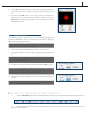
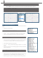
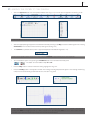
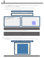
INSTRUCTION MANUAL
NTEGRA LIFE AND OLYMPUS IX71
COMBINED ATOMIC FORCE AND FLUORESCENCE MICROSCOPY
BY SKJOEDT, J. M. AND KLAUSEN, L. H. AND KNUDSEN, N.P.
2
1.0 PLEASE
READ!
THIS MANUAL ADDRESSES THE COMBINED OPERATION OF A NTEGRA LIFE AND OLYMPUS IX71 MICROSCOPE. THE
PROTOCOL IS WRITTEN TO OPERATORS WHICH ALREADY POSSESS A BASIC KNOWLEDGE CONCERNING ATOMIC
FORCE MICROSCOPY, AND MODERATE OPERATIONAL SKILLS FOR AN OLYMPUS IX71 MICROSCOPE.
BY SUBSTITUTING WITH ADDITIONAL DEVICES, THE SAFETY INFORMATION AND PROTOCOL OF SUCH DEVICES
SHOULD BE FOLLOWED INSTEAD. THE INSTRUMENT SHOULD ONLY BE USED BY OPERATORS WHO HAVE HAD A
CERTIFIED INTRODUCTION TO THE INSTRUMENT AND ANY QUESTIONS DURING USE SHOULD BE ADDRESSED TO
SUCH EXPERTS.
FOR FURTHER INFORMATION REGARDING ADVANCED OPERATION OF THE NTEGRA LIFE MICROSCOPE, EXPERTS OF
THE NT-MDT COMPANY SHOULD BE ADDRESSED.
2.0 GENERAL
SAFETY MEASURES
1. Be aware of safety signs when working with electric circuits.
Prior to working with the devise it must be grounded. Before
connecting or disconnecting controllers, the devise must be
turned off. Connecting or disconnecting controllers when
the device is working may lead to damage on the electrical
circuit and death of the device.
2. Check safety signs for operating with instruments having
laser radiation source. Do not stare into the beam. When
laser radiation is in progress, a red indicator on the
mechanical lid will be illuminated.
3. Do not disassemble any part of the device! Disassembling
of the product is permitted only for experts certified by the
company in question.
4. Do not connect additional devices to the instrument, without
advising with an expert.
5. Do not expose the device for powerful mechanical stress.
6. Protect the device from the effect of high temperatures and
liquid ingestion.
7. During operation the temperature of the lamp housing
(IX71) will become extremely high. Allow the housing 10
cm of free space around, especially above.
3
3.0
CONTENT
1.0
PLEASE READ! . . . . . . . . . . . . . . . . . . . . . . . . . . . . . . . . . . . . . . . . . . . . . . . . . . . . . . . . . . . . . . . . . . . . . . . . . . . . . . . . . . . . . . . . . . . . . . . . . . . . . . . . . . . . . . . . 2
2.0
GENERAL SAFETY MEASURES. . . . . . . . . . . . . . . . . . . . . . . . . . . . . . . . . . . . . . . . . . . . . . . . . . . . . . . . . . . . . . . . . . . . . . . . . . . . . . . . . . . . . . . . . . . . 2
4.0
THE NTEGRA LIFE AND OLYMPUS IX71 SETUP. . . . . . . . . . . . . . . . . . . . . . . . . . . . . . . . . . . . . . . . . . . . . . . . . . . . . . . . . . . . . . . . . . . . . . .4
5.0
PREPARING THE NTEGRA LIFE ATOMIC FORCE MICROSCOPE . . . . . . . . . . . . . . . . . . . . . . . . . . . . . . . . . . . . . . . . . . . . . . . . . . . 5
.
5.1
NTEGRA Life Control System. . . . . . . . . . . . . . . . . . . . . . . . . . . . . . . . . . . . . . . . . . . . . . . . . . . . . . . . . . . . . . . . . . . . . . . . . . . . . . . . . . . . . . . . . . . . . 5
5.2
Turning on the NTEGRA Life. . . . . . . . . . . . . . . . . . . . . . . . . . . . . . . . . . . . . . . . . . . . . . . . . . . . . . . . . . . . . . . . . . . . . . . . . . . . . . . . . . . . . . . . . . . . . 5
5.3
Control software interface. . . . . . . . . . . . . . . . . . . . . . . . . . . . . . . . . . . . . . . . . . . . . . . . . . . . . . . . . . . . . . . . . . . . . . . . . . . . . . . . . . . . . . . . . . . . . . . . 6
5.3.1
Hardware Parameter Panel. . . . . . . . . . . . . . . . . . . . . . . . . . . . . . . . . . . . . . . . . . . . . . . . . . . . . . . . . . . . . . . . . . . . . . . . . . . . . . . . . . . . . . . . . . . 6
5.3.2
Operation Modes Panel. . . . . . . . . . . . . . . . . . . . . . . . . . . . . . . . . . . . . . . . . . . . . . . . . . . . . . . . . . . . . . . . . . . . . . . . . . . . . . . . . . . . . . . . . . . . . . . 6
5.3.3
Advanced Operation Modes Panel. . . . . . . . . . . . . . . . . . . . . . . . . . . . . . . . . . . . . . . . . . . . . . . . . . . . . . . . . . . . . . . . . . . . . . . . . . . . . . . . . . 6
5.3.4
Slide-bars in Input Fields. . . . . . . . . . . . . . . . . . . . . . . . . . . . . . . . . . . . . . . . . . . . . . . . . . . . . . . . . . . . . . . . . . . . . . . . . . . . . . . . . . . . . . . . . . . . . 6
5.4
Installing the Probe . . . . . . . . . . . . . . . . . . . . . . . . . . . . . . . . . . . . . . . . . . . . . . . . . . . . . . . . . . . . . . . . . . . . . . . . . . . . . . . . . . . . . . . . . . . . . . . . . . . . . . . . 7
5.5
Mounting the Sample. . . . . . . . . . . . . . . . . . . . . . . . . . . . . . . . . . . . . . . . . . . . . . . . . . . . . . . . . . . . . . . . . . . . . . . . . . . . . . . . . . . . . . . . . . . . . . . . . . . . . . 8
5.6
Mounting the Sample Holder . . . . . . . . . . . . . . . . . . . . . . . . . . . . . . . . . . . . . . . . . . . . . . . . . . . . . . . . . . . . . . . . . . . . . . . . . . . . . . . . . . . . . . . . . . . . . 8
SEMICONTACT OPERATION OF THE NTEGRA LIFE. . . . . . . . . . . . . . . . . . . . . . . . . . . . . . . . . . . . . . . . . . . . . . . . . . . . . . . . . . . . . . . . . . . 9
6.0
6.1
Initial state. . . . . . . . . . . . . . . . . . . . . . . . . . . . . . . . . . . . . . . . . . . . . . . . . . . . . . . . . . . . . . . . . . . . . . . . . . . . . . . . . . . . . . . . . . . . . . . . . . . . . . . . . . . . . . . . . . . 9
6.2
Setting the AFM for working in SemiContact Mode. . . . . . . . . . . . . . . . . . . . . . . . . . . . . . . . . . . . . . . . . . . . . . . . . . . . . . . . . . . . . . . . . . . 9
6.3
Adjustment of the Optical Deflection System. . . . . . . . . . . . . . . . . . . . . . . . . . . . . . . . . . . . . . . . . . . . . . . . . . . . . . . . . . . . . . . . . . . . . . . . . . 9
6.3.1
Turning on the Laser. . . . . . . . . . . . . . . . . . . . . . . . . . . . . . . . . . . . . . . . . . . . . . . . . . . . . . . . . . . . . . . . . . . . . . . . . . . . . . . . . . . . . . . . . . . . . . . . . . 9
6.3.2
Aligning the Laser Beam onto the Cantilever. . . . . . . . . . . . . . . . . . . . . . . . . . . . . . . . . . . . . . . . . . . . . . . . . . . . . . . . . . . . . . . . . . . . . . 9
6.3.2.1
6.3.3
6.4
The Five Steps of Alignment. . . . . . . . . . . . . . . . . . . . . . . . . . . . . . . . . . . . . . . . . . . . . . . . . . . . . . . . . . . . . . . . . . . . . . . . . . . . . . . . . . .10
Working in liquid. . . . . . . . . . . . . . . . . . . . . . . . . . . . . . . . . . . . . . . . . . . . . . . . . . . . . . . . . . . . . . . . . . . . . . . . . . . . . . . . . . . . . . . . . . . . . . . . . . . . . .11
Setting the Cantilever Working Frequency. . . . . . . . . . . . . . . . . . . . . . . . . . . . . . . . . . . . . . . . . . . . . . . . . . . . . . . . . . . . . . . . . . . . . . . . . . . . .11
6.4.1
Creating a New Probe File. . . . . . . . . . . . . . . . . . . . . . . . . . . . . . . . . . . . . . . . . . . . . . . . . . . . . . . . . . . . . . . . . . . . . . . . . . . . . . . . . . . . . . . . . .12
6.5
Landing the Probe to the Sample. . . . . . . . . . . . . . . . . . . . . . . . . . . . . . . . . . . . . . . . . . . . . . . . . . . . . . . . . . . . . . . . . . . . . . . . . . . . . . . . . . . . . . .13
6.6
Setting the Feedback Gain Working Level . . . . . . . . . . . . . . . . . . . . . . . . . . . . . . . . . . . . . . . . . . . . . . . . . . . . . . . . . . . . . . . . . . . . . . . . . . . .14
6.7
Setting the Scanning Parameters. . . . . . . . . . . . . . . . . . . . . . . . . . . . . . . . . . . . . . . . . . . . . . . . . . . . . . . . . . . . . . . . . . . . . . . . . . . . . . . . . . . . . . .14
6.7.1
Setting the Scan Size, Point Number and Step Size . . . . . . . . . . . . . . . . . . . . . . . . . . . . . . . . . . . . . . . . . . . . . . . . . . . . . . . . . . . . .15
6.7.1.1
Scan Size. . . . . . . . . . . . . . . . . . . . . . . . . . . . . . . . . . . . . . . . . . . . . . . . . . . . . . . . . . . . . . . . . . . . . . . . . . . . . . . . . . . . . . . . . . . . . . . . . . . . . . . . . . 15
6.7.1.2
Point Number. . . . . . . . . . . . . . . . . . . . . . . . . . . . . . . . . . . . . . . . . . . . . . . . . . . . . . . . . . . . . . . . . . . . . . . . . . . . . . . . . . . . . . . . . . . . . . . . . . . . .15
6.7.1.3
Step Size. . . . . . . . . . . . . . . . . . . . . . . . . . . . . . . . . . . . . . . . . . . . . . . . . . . . . . . . . . . . . . . . . . . . . . . . . . . . . . . . . . . . . . . . . . . . . . . . . . . . . . . . . .15
6.7.2
Setting the Scan Rate. . . . . . . . . . . . . . . . . . . . . . . . . . . . . . . . . . . . . . . . . . . . . . . . . . . . . . . . . . . . . . . . . . . . . . . . . . . . . . . . . . . . . . . . . . . . . . . 15
6.7.3
Setting the Scan Direction . . . . . . . . . . . . . . . . . . . . . . . . . . . . . . . . . . . . . . . . . . . . . . . . . . . . . . . . . . . . . . . . . . . . . . . . . . . . . . . . . . . . . . . . . . 15
6.7.4
Setting the Scan Signal. . . . . . . . . . . . . . . . . . . . . . . . . . . . . . . . . . . . . . . . . . . . . . . . . . . . . . . . . . . . . . . . . . . . . . . . . . . . . . . . . . . . . . . . . . . . . 16
6.8
Scanning in SemiContact Mode. . . . . . . . . . . . . . . . . . . . . . . . . . . . . . . . . . . . . . . . . . . . . . . . . . . . . . . . . . . . . . . . . . . . . . . . . . . . . . . . . . . . . . . . .16
6.8.1
Scan Launch. . . . . . . . . . . . . . . . . . . . . . . . . . . . . . . . . . . . . . . . . . . . . . . . . . . . . . . . . . . . . . . . . . . . . . . . . . . . . . . . . . . . . . . . . . . . . . . . . . . . . . . . . . 16
6.8.2
Alterations of Parameters in the Process of Scanning. . . . . . . . . . . . . . . . . . . . . . . . . . . . . . . . . . . . . . . . . . . . . . . . . . . . . . . . . .16
6.8.3
Optimizing Parameters During the Process of Scanning. . . . . . . . . . . . . . . . . . . . . . . . . . . . . . . . . . . . . . . . . . . . . . . . . . . . . . . . 17
6.8.4
Image an Alternative Region Using the Previous Frame . . . . . . . . . . . . . . . . . . . . . . . . . . . . . . . . . . . . . . . . . . . . . . . . . . . . . . . . 17
6.8.5
Scan Another Location by Sample Movement . . . . . . . . . . . . . . . . . . . . . . . . . . . . . . . . . . . . . . . . . . . . . . . . . . . . . . . . . . . . . . . . . . . .18
...
6.9
Saving and Viewing the Obtained Results . . . . . . . . . . . . . . . . . . . . . . . . . . . . . . . . . . . . . . . . . . . . . . . . . . . . . . . . . . . . . . . . . . . . . . . . . . . . .18
6.10
Shutting Down the NTEGRA Life. . . . . . . . . . . . . . . . . . . . . . . . . . . . . . . . . . . . . . . . . . . . . . . . . . . . . . . . . . . . . . . . . . . . . . . . . . . . . . . . . . . . . . .18
7.0
COMBINED ATOMIC FORCE AND LIGHT MICROSCOPY. . . . . . . . . . . . . . . . . . . . . . . . . . . . . . . . . . . . . . . . . . . . . . . . . . . . . . . . . . . . .19
7.1
Preparing the Olympus IX71 Inverted Light Microscope. . . . . . . . . . . . . . . . . . . . . . . . . . . . . . . . . . . . . . . . . . . . . . . . . . . . . . . . . . . . . 19
7.1.1
Olympus IX71 Control System . . . . . . . . . . . . . . . . . . . . . . . . . . . . . . . . . . . . . . . . . . . . . . . . . . . . . . . . . . . . . . . . . . . . . . . . . . . . . . . . . . . . . .19
7.1.2
Turning on the Apparatus. . . . . . . . . . . . . . . . . . . . . . . . . . . . . . . . . . . . . . . . . . . . . . . . . . . . . . . . . . . . . . . . . . . . . . . . . . . . . . . . . . . . . . . . . . .19
7.1.3
Mounting Samples. . . . . . . . . . . . . . . . . . . . . . . . . . . . . . . . . . . . . . . . . . . . . . . . . . . . . . . . . . . . . . . . . . . . . . . . . . . . . . . . . . . . . . . . . . . . . . . . . . . .19
7.1.4
Control Software Interface. . . . . . . . . . . . . . . . . . . . . . . . . . . . . . . . . . . . . . . . . . . . . . . . . . . . . . . . . . . . . . . . . . . . . . . . . . . . . . . . . . . . . . . . . 20
7.2
Aligning Probe, Sample and Objective. . . . . . . . . . . . . . . . . . . . . . . . . . . . . . . . . . . . . . . . . . . . . . . . . . . . . . . . . . . . . . . . . . . . . . . . . . . . . . . . 20
7.3
Setting up 60x Magnification. . . . . . . . . . . . . . . . . . . . . . . . . . . . . . . . . . . . . . . . . . . . . . . . . . . . . . . . . . . . . . . . . . . . . . . . . . . . . . . . . . . . . . . . . . . 22
7.4
Capturing Fluorescence images. . . . . . . . . . . . . . . . . . . . . . . . . . . . . . . . . . . . . . . . . . . . . . . . . . . . . . . . . . . . . . . . . . . . . . . . . . . . . . . . . . . . . . . . 23
7.5
Combining AFM topology and Fluorescence image . . . . . . . . . . . . . . . . . . . . . . . . . . . . . . . . . . . . . . . . . . . . . . . . . . . . . . . . . . . . . . . . . 23
4
4.0 THE
NTEGRA LIFE AND OLYMPUS IX71 SETUP
NTEGRA Life Atomic Force Microscope (NT-MDT Co, Moscow, Russia), mounted on an OLYMPUS IX71 inverted light microscope
(Olympus, Hamburg, Germany). These are mounted on a TS-150 active vibration-isolation system (Stable Table, Ammerbuch,
Germany).
FIG. 4 1: MAIN SETUP COMPONENTS OF NTEGRA LIFE AND OLYMPUS IX71:
1 – MECHANICAL LID; 2 – MEASUREMENT HEAD; 3 – OLYMPUS IX71; 4 – ACTIVE VIBRATION-ISOLATION SYSTEM; 5 –
MECHANICAL LID CONTROLLER
5
5.0 PREPARING
THE NTEGRA LIFE ATOMIC FORCE MICROSCOPE
5.1 NTEGRA LIFE CONTROL SYSTEM
The NTEGRA Life control system includes:
-
NTEGRA Life controller (Fig. 5 1)
-
Control PC
Both controller and PC can be found beneath the monitors next to
the NTEGRA Life microscope.
-
Mechanical lid controller (Fig. 5 2)
The mechanical lid controller is positioned beside the NTEGRA
Life microscope. The black up/down regulator are held in place by
magnets, which means it can be moved by the operator, if needed.
FIG. 5-1
FIG. 5-2
FIG. 5-2
FIG. 5-2
5.2 TURNING ON THE NTEGRA LIFE
•
•
Turn on the power supply by clicking the main switch on
the front panel. The switch light will become red and the
display on the NTEGRA Life will turn on
Turn on the unit controlling the mechanical lid, with the
switch located on the backside. A blue light will appear on
the front of the unit.
•
Turn on the control PC with the switch located on the front
panel.
•
Double click on the shortcut named Nova_Px
on the desktop.
•
Upon launching, the control software will perform an
Initialization of the device, which determines the state of it.
The result of this initialization may be one of two outcomes.
located
-
The SPM is initializing, determining device state.
-
Initialization successful.
The device is ready for use.
-
Device is not turned on.
6
5.3 CONTROL SOFTWARE INTERFACE
The basic components of the Nova control software interface (Fig. 5 3):
•
Main Menu
•
Hardware Parameters
•
Operation Modes
•
Advanced Operation Modes
•
Filter Script Shortcuts
•
Initialization (status bar)
FIG. 5-3
5.3.1 [ H ARD WA R E PA R A M E TE R PA N E L ]
The Hardware Parameter panel features the most frequently used controls of the software. The panel contains functions like the working
mode of the AFM, the laser control, signal type and measurement etc.
5.3.2 [ O P E R AT IO N M O D ES PA N E L ]
The buttons of the operation modes panel are shortcuts for quickly launching and changing between different working windows. Some
are more frequently used than others, and the following five are required for basic use of the AFM.
•
Aiming
•
Resonance
•
Approach
•
Scanning
•
Camera
5.3.3
FIG. 5-4
[ AD VAN C E D O P E R AT I O N M O D ES PA N E L ]
The buttons of the advanced operation modes panel is for more advanced users only, and is not really necessary for basic use. For further
information regarding this panel, see the user manual provided by the manufacturer.
5.3.4
[ S L ID E -B A R S I N I N P U T F I E L D S ]
Changing variables in the Hardware Parameter panel and in sub-windows of the operation modes can be done in two ways:
•
Simply mark the parameter value in the input field and then substitute it with the desired value.
•
Activate a slide-bar by double-clicking the mouse on an input field. A slide-bar similar to the one seen in fig. 6.4 will appear. By using
the mouse cursor the input value can now be changed.
FIG. 5-5
Notice: To increase/decrease the value interval, press ALT while using the mouse cursor to set the desired interval (blue lines). When
releasing the ALT button the slide-bar will show the new selected interval.
7
5.4 INSTALLING THE PROBE
To install or replace a probe, do the following:
•
Put the mechanical lid into the upmost position in order to gain access
to the prism, using the mechanical lid controller.
•
Place the prism removal tool around the prism and turn it gently
clockwise until the prism detaches from the lid, as seen from Fig. 5 6.
•
The prism should be placed upside-down on a lens paper, like seen
in Fig. 5 7
•
Take a probe from the box with an AFM approved tweezers (Fig. 5 8)
making sure that the cantilever is directed towards you.
FIG. 5-6
Notice: Do not turn over the cantilever, since the probes are placed
with their tips pointing upwards.
•
Pull the prism spring with thumb and index finger of your free hand
and place the probe beneath the spring. A proper cantilever placement
can be seen in Fig. 5 9.
FIG. 5-6
Notice: Pulling the spring too hard could permanently damage the
spring.
Notice: The probe should be placed as far out on the prism as possible,
while maintaining the proper attachment by the spring.
•
Place the prism, with the probe pointing downwards, into the prism
removal tool. The prism should be placed in the holder with the kink
(red arrow) facing towards you and the cutes in the metal ring (green
arrows) facing to your right and left, respectively, like seen in Fig. 5 10.
•
The prism is inserted back into the holder (Fig. 5 11), still with the kink
facing towards you, and turn it counter-clockwise to fasten.
FIG. 5-7
Notice: DO NOT use any unnecessary force! When the correct fit is
found, the prism will slide in easily.
FIG. 5-8
FIG. 5-9
FIG. 5-10
FIG. 5-11
8
5.5 MOUNTING THE SAMPLE
Together with the NTEGRA Life microscope, three different types of
sample holders are provided. Two of these give the possibility to mount
micro wells (Fig. 5 12) and the third to use standard microscope glass
slides.
FIG. 5-12
LARGE WELLS
FIG. 5-13
FIG. 5-14
(MOUNTING DIAMETER 50 MM)
•
SMALL WELLS
GLASS SLIDES
FIG. 5-15
(MOUNTING DIAMETER 35 MM)
(75 MM X 25 MM)
Place the selected well into its proper sample holder. Fix the well by turning the concomitant locking ring clockwise.
Notice: Be aware that both springs on the locking ring are properly attached into the gaps on the sample holder.
•
Place the glass slide in the glass slide sample holder. Fix the slide by placing the springs, see Fig. 5 15, on top of the mounted
slide and fasten the screws.
Notice: When sliding the springs over the sample, keep in mind that it may touch the specimen deposited onto the slide.
5.6 MOUNTING THE SAMPLE HOLDER
All types of sample holders are mounted into the microscope in the same way. Three magnetic attachment points (red arrows) are
used to keep the sample holder in place, as seen on Fig. 5 16. The sample holder is lowered into the microscope by using the two
finger holes in the sample holders, indicated in Fig. 5 17.
FIG. 5-16
FIG. 5-17
Notice: Before mounting the sample holder into the microscope, make sure that the selected objective is lowered into its lowest
position, to avoid damaging the objective.
Notice: Keep in mind that if a probe has been mounted, it is easy to destroy the cantilever by touching it with the back of your hand.
Notice: If scanning in liquid, medium should be added before closing the mechanical lid, since injection during operation is difficult.
9
6.0 S E M I C O N TA C T
O P E R AT I O N O F
THE NTEGRA LIFE
6.1 INITIAL STATE
Prior to the setup for SemiContact AFM it is assumed that the following initial state demands have been completed:
•
The instrument has been turned on, including the launch of control software, of which the main control interface is displayed.
(sec. 5.2)
•
The probe has been mounted onto the prism and placed back into the prism holder. (sec. 5.4)
•
The sample has been mounted into the sample holder, and placed into the AFM. (sec. 5.5)
6.2 SETTING THE AFM FOR WORKING IN SEMICONTACT MODE
From the Hardware Parameter panel select the SemiContact mode of the
working mode selection submenu (Fig. 6 1).
FIG. 6-1
Notice: When setting the working mode to SemiContact, the instrument automatically sets the appropriate settings for working in
SemiContact mode, like setting the signal to Mag.
6.3 ADJUSTMENT OF THE OPTICAL DEFLECTION SYSTEM
6.3.1
[ T URN IN G O N T H E L A S E R ]
The turning On and Off, of the laser, is controlled in the Hardware Parameter panel by pressing the Laser button. (In Fig. 6 2 the laser
is turned on)
FIG. 6-2
/
- The On/Off state of the laser.
Notice: By default, the Laser button is turned On, upon launching the software.
Notice: The Laser condition is indicated by a light on the front panel of the AFM, which is blue when the laser is Off and red when it
is On.
Notice: The laser automatically turns Off when the mechanical lid is raised, meaning that the risk of direct eye contact is minimized.
However, DO NOT stare directly into the laser beam, since this can cause permanent damage to the eyes!
6.3.2
[ ALIGNING THE LASER BEAM ONTO THE CANTILEVER ]
1. Select the Aiming button from the Operation Modes panel (Fig. 6 3). This will open the Aiming window (Fig. 6 4) and will most often
show “Laser out of area!”.
FIG. 6-3
10
The Aiming Window contains an indicator of the laser spot position, relative
to the four detectors of the photodiode and three signals, which have the
following meaning:
DFL The difference in signal between top and bottom halves of the photodiode.
LF
The difference in signal between left and right halves of the
photodiode.
Laser The total signal of all four segments of photodiode, which is
proportional to intensity of laser
reflected from the cantilever.
FIG. 6-4
Notice: The Laser and photodiode can be moved manually with the
LaserX, LaserY, DiodeX and DiodeY buttons. This is however not
necessary, since the NTEGRA Life and the Nova software is capable of
doing a semi-automatic alignment.
2. Press the Alignment button at the top of the Aiming Window. This will
display the Alignment window (Fig. 6 5).
Notice: It is assumed that the alignment is performed on a sample in air.
Notice: The Alignment window plots the Laser signal relative to the
movement, in the XY-plan, of the laser.
6.3.2.1
[ THE FIVE STEPS OF ALIGNMENT ]
FIG. 6-5
The purpose of this alignment is to steer the laser spot onto the end of the
cantilever. The following two functions are often very helpful for locating
the cantilever:
Activates the Manual Probe Movement function. Left-click in the
scan area, at the desired position, followed by a right-click and
selection of “move to position”.
Activates the Area Select function. By press-holding Ctrl it is
possible to drag a smaller scan area by left-clicking and dragging
the cursor across the screen.
In order to gain a rough idea about the probe position it is often very
timesaving to follow The Five Steps of Alignment (Fig. 6 6):
•
Using the Manual Probe Movement function, move the laser to the
bottom left of the scan area.
•
If the chip has not already been located by a sudden increase in Laser
signal, move the laser to the right along the x-axis until the left edge
of the chip is located.
•
Move the laser parallel to the chip edge, until the top edge of the chip
is located.
•
Move the laser to the top right corner of the chip.
•
Using the Area Select function a scan area should be launched from
this point. The scan area should include some of the chip and a larger
area to the right of the cantilever. An example of such an area can be
seen in Fig. 6 7.
FIG. 6-6
FIG. 6-7
11
3. Use the Manually Move function to move the laser to the peak reflection of
the cantilever, which is the highest Laser signal outside the chip (see Fig.
6 7).
4. By pressing the Auto button in the Aiming window, the software will
physically move the cantilever to the local peak in reflection and set the
DFL and LF as close to zero as possible. The Aiming window will then look
something like Fig. 6 8.
FIG. 6-8
6.3.3
[ WORKING IN LIQUID ]
If investigating a sample in liquid medium, it is recommended that the alignment
of laser and photodiode is done in air, following The Five Steps of Alignment,
before submerging the probe in liquid.
Notice: The cantilever position, in the Alignment window, will shift due to the
different refractive index of liquid compared to air.
1. Follow The Five Steps of Alignment of the laser in air, see sec. 6.3.
2. Submerge the probe in your liquid medium, by gently closing the mechanical
lid.
Notice: Make sure that the probe is completely submerged, and that there
are no air-bubbles between probe and prism or around the cantilever. This is
verified by using the Olympus IX71.
3. In the top of the Alignment window, select liquid and press Run (Fig. 6 9).
Notice: The software will NOT provide a message saying that the movement is
complete, but while the movement is being performed, the rest of the buttons
in the Alignment window will be unpressable. (Fig. 6 10)
FIG. 6-9
4. Follow the Five Steps of Alignment one more time, and the alignment is
complete.
Notice: When completing operation with liquid medium, REMEMBER TO
MOVE THE PHOTODIODE BACK TO AIR POSITION!
FIG. 6-10
6.4 SETTING THE CANTILEVER WORKING FREQUENCY
a.
Select the Resonance button from the Operation Modes panel (Fig. 6 3). This will open the Resonance window (Fig. 6 12).
FIG. 6-11
b.
Select the appropriate probe file from the Probes dropdown menu, see Fig. 6 13. If the file does not exist, go to sec. 6.4.1
Creating a New Probe File.
12
Notice: The ProbeDefault file can be used in most cases (imaging in air), but for more frequently used cantilevers it is recommended
that a probe file is created.
By pressing Run the frequency is automatically tuned and set to a magnitude of approximately 10 (Fig. 6 14).
c.
Notice: The Amplitude and Phase Adjust buttons can be used to readjust the amplitude and phase, to correct for small
variations.
Notice: If the frequency signal is noisy, noise reduction filters can be applied. The Scripts Filter shortcuts are located in the Main
window of the Nova software. The default noise filter is set to 250.
FIG. 6-13
FIG. 6-12
6.4.1
FIG. 6-14
[ CREATING A NEW PROBE FILE ]
The addition of new probe files should only be performed by advanced users (Leonid or
Peter).
•
Close down the control software.
Notice: Prior alignment of the laser will NOT be lost.
•
Go to the “…Nova_Px_66\Storage\Probes” subfolder of the software directory.
•
Copy one of the old probe files and rename it according to your cantilever.
FIG. 6-15
Notice: Keep the .ini extension.
•
Edit the probe file with a text editing program, and insert the information provided by
the manufacturer. (ID, FreqMin, FreqMax and ForceConstant) (see Fig. 6 15)
•
Save the applied changes to the same directory.
•
Go to the “…Nova_Px_66\Devices\Bio\Storage” subfolder of the software
directory.
•
Open the file FreqAdjust.ini with a text editing program and scroll to the very bottom
of the file. (see Fig. 6 16)
Notice: DO NOT start editing the file without making a backup. Unwanted changes
could result in the malfunctioning of the software.
FIG. 6-16
•
Add the name of your newly created probe file at the bottom of the list and increase
the “ProbesCount” by +1 (with the addition of two new probe files, +2 etc.)
•
Restart the program and go to sec. 6.4 Setting the Cantilever Working Frequency.
13
6.5 LANDING THE PROBE TO THE SAMPLE
Select the Approach button from the Operation Modes Panel (Fig. 6 17). This will open the Approach window (Fig. 6 18).
•
FIG. 6-17
FIG. 6-18
FIG. 6-19
Notice: The Way parameter can be reset to zero by double-clicking it.
•
Select the appropriate signal type from the Hardware Parameter panel (Fig. 5 5). Mag is set as the default signal when choosing
SemiContact, which is also the most commonly used signal. (see Fig. 6 19)
•
The SetPoint is by default set to 5, which is approximately 50% of the default magnitude (~10).
FIG. 6-20
Notice: A more gentle contact can be achieved by setting the SetPoint to approximately 70% of the magnitude.
Turn the feedback system on by pressing the FeedBack button in the Hardware Parameter panel.
•
/ - This button turns the feedback loop On or Off
•
Press the Mag button in order to monitor the landing, highlighted in Fig. 6 21.
•
Press the Landing button in the Approach window. The message “Landing Complete” will appear in the message window (Fig.
6 22) and a successful landing should look like the curve seen in Fig. 6 23.
FIG. 6-21
FIG. 6-22
FIG. 6-23
Notice: The Y-axis can be dragged up and down, by pressing it with the cursor. The interval can be increased or decreased by
holding down Shift and dragging the axis up or down, using the cursor. By holding down Ctrl, the cursor can be used to mark the
two limits of the desired interval and upon release the selected interval will appear.
14
6.6 SETTING THE FEEDBACK GAIN WORKING LEVEL
1. Select the Approach button from the Operation Modes Panel (Fig. 6 24). This will open the Approach window (Fig. 6 25).
2. Plot the magnitude signal by pressing the Mag button
3. Double-click on the Gain input field in the Hardware Parameter panel, which will open the slide-bar (Fig. 6 26).
4. Increase the Gain until the signal begins to oscillate (Fig. 6 27).
FIG. 6-24
FIG. 6-26
FIG. 6-25
FIG. 6-27
Notice: At high gain, the feedback loop will react to even the smallest height differences, whereas at low gain, a low feedback
response will be obtained. When the gain becomes too high, the system begins to self-oscillate, which can be seen as a noisy
magnitude signal.
5. Decrease the gain to approximately 60-70% of the self-oscillation threshold level.
Notice: If the signal starts oscillating as soon as the landing is complete, and if the noise cannot be reduced simply by decreasing
the gain, this could be caused by a so called “sticking” effect. This phenomenon can be reduced by increasing the oscillation
amplitude (The amplitude parameter can be found by pressing the Scheme button on the Main Operations panel, but this should
only be done by certified users).
6.7 SETTING THE SCANNING PARAMETERS
Select the Scanning button from the Operation Modes panel (Fig. 6 28). This will open the Scanning window seen in Fig. 6 29.
FIG. 6-28
FIG. 6-29
Notice: The Aiming, Resonance and Approach settings can all be applied from the Quick panel of the Scanning window.
15
6.7.1
[ SETTING THE SCAN SIZE, POINT NUMBER AND STEP SIZE ]
Select the Area Select button from the top of the Scan window (Fig. 6 29).
This will open the Scan Area Selection window (Fig. 6 30). The scan area can
be moved by dragging the red square with the cursor.
Notice: The scan area is set to be rectangular by default (X=Y), which can
be changed by clicking it.
Notice: The Center values determine the coordinates of the scan area. It
should be noted that the coordinates change when altering the Scan Size.
6.7.1.1
FIG. 6-30
[ SCAN SIZE ]
The Scan Size determines the dimensions of the scan area in units of
micrometers (µm). The default value is 10 µm x 10 µm, but can be changed as
the user sees fit. The dimensions of the Scan Size can be seen in comparison
to the maximal scan area indicated by the red square to the left of the Area
Selection window, and be moved around by dragging it with the mouse.
6.7.1.2
[ POINT NUMBER ]
The Point Number determines the amount of points measured in the X- and
Y-direction of a selected scan area. This yields the resolution of the scanned
image, and is by default set to 512 x 512.
6.7.1.3 [ STEP SIZE ]
The Step Size is a result of the Scan Size and the Point Number: Step
Size = (Scan Size)/(Point Number)
Notice: The Scan Size, Point Number and Step Size are three interdependent values. As can be seen the Scan Size and Step Size have a blue
background while the Point Number has a yellow background. This means
that the Point Number is held constant, and if changing the Scan Size, only
the Step Size will change with it. The value which should be held constant
can be changed by clicking the name of the variable.
6.7.2
[ SETTING THE SCAN RATE ]
Set the Scan Rate in the top panel of the Scan Window (Fig. 6 31). The unit
of the scan rate can be defined as the frequency (Hz) of line scanning, or as
the velocity (µm/sec) of the tip relative to the surface, or as the scan time
(sec) required capturing the total area or the time interval between the data
acquisition of two adjacent points time/point (msec/Pnt). The scan rate is by
default set to frequency, usually in the range of 0.5 – 2 Hz, which is a good
starting point for most samples.
Notice: The optimal scan speed is highly dependent of the surface
properties of the sample which is being imaged. With rigid structures it is
possible to get good resolutions with high scan speeds, while slower scan
speeds are required for samples with large or soft structures.
FIG. 6-31
Notice: More experienced user will find it more comfortable to define the
scan rate in units of µm/s instead of Hz, especially when working with
fragile samples. When increasing the scan area, while the scan rate is set
to Hz, the actual scan speed will increase with the scan area. This could
damage both sample and tip.
6.7.3
[ SETTING THE SCAN DIRECTION ]
Select the Direction button from the top panel of the Scan window (Fig. 6
29). The scan direction can be selected from a dropdown menu (Fig. 6 32).
The software is by default set to scan from the bottom left corner and scanning
towards the right.
FIG. 6-32
16
6.7.4
[ SETTING THE SCAN SIGNAL ]
Select the Settings button from the top panel of the Scan window
(Fig. 6 29). This will show the Scan Settings window, from which
the number and type of signal can be selected (Fig. 6 33). Eight
different signals can be measured at the same time and the signal
can be chosen from a total of 28 options, of which some can be seen
in Fig. 6 34.
Select the Direction of each measurement; choose between the
forward or backwards scan.
Notice: It is recommended to have a measurement of the
measured signal and a height profile of both the forward and
backwards scan. The comparison of these will determine the
validity of the image captured.
Notice: The choice of signals can be saved by setting the signals
and pressing “Save As”.
FIG. 6-33
FIG. 6-34
6.8 SCANNING IN SEMICONTACT MODE
Once all the preparatory operations are performed; adjusting laser, finding resonance frequency, landing to the sample, choosing set
point and setting all the scan parameters, the actual scanning of the surface can be initiated.
6.8.1
[ SCAN LAUNCH ]
Press the Run button in the top left corner of the Scan window (Fig. 6 35).
FIG. 6-35
/
- This button starts and stops the scanning progress
Notice: If the Cyclic button
is pressed, the frames will be measured continuously, meaning that when one frame is completed, the
next frame is captured in the opposite direction.
The tip will start scanning the sample one line at a time, and display the measured data as a line in the image (Fig. 6 36).
The height profiles can be displayed by pressing the
to line 324 of Fig. 6 36 can be seen in Fig. 6 37.
button at the bottom left of each signal window. The height profile corresponding
FIG. 6-37
FIG. 6-36
FIG. 6-38
When scanning is completed, press the Stop button, located where the Run button was prior to scanning (Fig. 6 38).
6.8.2
[ ALTERATIONS OF PARAMETERS IN THE PROCESS OF SCANNING ]
If the height profile is tilted, which is often the case, it is possible to perform different subtractions during measurements in order to flatten
the signal. The height profile in Fig. 6 37 is currently not applied any subtractions, indicated by the button in the bottom right corner, which
is set to
. It can however be set to subtract both a plane, surf 2, 1st, 2nd, 3rd and 4th – order curves to improve the profiles.
17
FIG. 6-39
FIG. 6-40
When applying a 1st order subtraction to Fig. 6 37, the height profile is subtracted with the first order derivative and will instead look like
Fig. 6 40.
6.8.3
[ OPTIMIZING PARAMETERS DURING THE PROCESS OF SCANNING ]
The scan parameters set prior to scanning are generally not optimal for creating images of high quality. Scan parameters like the Scan
Rate (Fig. 6 41), SetPoint (Fig. 6 42) and Gain (Fig. 6 42) often need to be optimized. All of these can be changed while scanning.
FIG. 6-41
FIG. 6-42
The Pause button
, located at the top left corner of the scan panel (Fig. 6 41), is intended for this purpose. By pressing this button,
the tip will scan the same line over and over again. The plotting of lines in the 2D plot will stop, but the height profile for each line will
still be shown. This means that the only changes on the height profile are caused by the Scan Rate, SetPoint and/or Gain adjustments,
since the tip is scanning the same line over and over again.
The current image can be resumed by pressing the Pause button again, or a new frame with the newly set parameters can be obtained
by pressing the Restart button
.
6.8.4
[ IMAGE AN ALTERNATIVE REGION USING THE PREVIOUS FRAME ]
During scans it is often necessary to adjust the focus of the scan to either a smaller or larger region of the original scan.
•
Press the Area Select button
in the tool bar of the Scan window.
Notice: If the region you want to scan is larger than the previous frame, you need to press the Zoom Out button
•
Select the area you want to focus on by dragging a region with the mouse (see Fig. 6 43).
Notice: The selection of a new area will not affect the current scan.
•
Press the Restart button
to scan the selected region.
FIG. 6-43
.
18
6.8.5
[ SCAN ANOTHER LOCATION BY SAMPLE MOVEMENT ]
If you want to move the scan area to a completely new part of the sample,
it can be done in the following manner.
•
Press the Camera button in the Main Operations panel (Fig. 6 44).
This will open the Camera window (Fig. 6 45).
Notice: Do not perform any movement while the tip is in contact with
the surface, since this could crash the tip into the sample.
•
Press the ProbeX and ProbeY buttons to move the probe relative
to the sample or press the StageX and StageY to move the sample
relative to the probe.
Notice: The movement of probe and stage can be monitored using the
Olympus IX71.
FIG. 6-45
FIG. 6-44
6.9 SCANNING IN SEMICONTACT MODE
The control software saves the acquired data in the “…Nova_Px_66\
Data” subfolder of the software directory with regular time intervals.
It is however recommended that the data is saved manually while
acquiring.
•
Press the File button in the Main Menu panel and select either
Save or Save as (Fig. 6 46).
•
In order to view the current Scan File or see a previously saved
file, press the Data button in the Main Operations Panel (Fig. 6
47), this will open the Image Analysis window (Fig. 6 48)
Notice: Image Analysis window gives the basic tools for AFM
image analysis and editing.
FIG. 6-46
FIG. 6-48
FIG. 6-47
6.10 SHUTTING DOWN THE NTEGRA LIFE
When AFM imaging has been completed do the following before
turning of the instrument.
•
Open the Approach window, by selecting the Approach button
from the Operation Modes panel (Fig. 6 17).
•
Press the Remove (Move) button from the Approach Panel
(Fig. 6 18) and retract the probe 2-3 mm. You can follow the
retraction in the Way parameter.
Notice: The Way parameter can be reset to zero by double-clicking
it.
FIG. 6-50
•
Turn off the feedback loop by pressing the Feedback button
...
/
.
•
Close down the program and turn off the instrument.
FIG. 6-49
19
7.0
COMBINED ATOMIC FORCE AND
LIGHT MICROSCOPY
THE FOLLOWING DESCRIPTION REQUIRES THAT THE NTEGRA LIFE MICROSCOPE IS READY FOR OPERATION, SEE
SEC. 5 PREPARING THE NTEGRA LIFE ATOMIC FORCE MICROSCOPE, AND THAT THE OPERATOR POSSESSES A BASIC
KNOWLEDGE OF THE NTEGRA LIFE MICROSCOPE. FOR INTRODUCTION TO BASIC FLUORESCENCE IMAGING, PLEASE
READ THE MANUFACTURE MANUAL.
7.1 PREPARING THE OLYMPUS IX71 INVERTED LIGHT MICROSCOPE
7.1.1
[ OLYMPUS IX71 CONTROL SYSTEM ]
The Olympus IX71 control system includes:
•
IX71 light source (Fig. 7 1)
•
Control PC
Both fluorescence light source and PC can be found beneath the monitors next to the IX71 microscope.
•
Bright Field (BF) light source (Fig. 7 2)
FIG. 7-1
7.1.2
FIG. 7-2
[ TURNING ON THE APPARATUS ]
Turn on the radiation supply by clicking the main switch on the front panel of the fluorescence light source. The switch light will become
green and the life time counter will begin.
Notice: The light source should only be turned on when one is ready to use it, to
increase life time of the lamp. The light source should never be turned off until
completely finished or absent from the microscope for longer than 2 hours. Use
instead the shutter to avoid excitation of fluorescence specimens. After turning off
the lamp, leave off for at least 30 minutes.
•
Turn on the controller PC with the switch located on the front.
•
Double click on the shortcut named DP Controller
•
Objectives should be mounted in the objective unit (Fig. 7 3).
7.1.3
located on the desktop.
FIG. 7-3
[ M O U N T I N G S A MP L ES ]
All three types of sample holders can be used for fluorescence imaging. The sample holders are mounted as described in sec. 5.5.
•
Dry imaging: Samples can be prepared in advance and no further modification is necessary.
•
Liquid imaging: Dyes or fluorescence specimens should be added to the sample prior to scanning with the atomic force microscope,
due to the mechanical lid making injection to the sample during operation difficult.
Notice: A low magnifying objective should be chosen for the pre-alignment of probe, sample and objective.
20
Notice: Remember to reduce the objective platform to its ground-state before closing down the mechanical lid.
Notice: The probe should be retracted far enough before closing the mechanical lid. Be aware when changing from wells to microscopic
slide, that the probe should be retracted significantly more than when changing from large to small wells.
7.1.4
[ C O N T RO L S O F T WA R E I N T E R FA CE ]
The DP Control interface has several components (seen in Fig. 7 4):
•
Capture
•
Preview
•
Color
•
Level
•
Scale
•
Timelapse/Movie
•
Microscope
•
Image Quality
Only the capture mode will be used in this protocol. For further information of the other modes see user manual provided by manufacture.
FIG. 7-4
7.2 ALIGNING PROBE, SAMPLE AND OBJECTIVE
Before scanning and capturing images, the probe, sample and selected objective should be aligned. This is most easily done in the
following way:
Notice: Both the NTEGRA Life and Olympus IX71 microscopes should be operational and a sample should be mounted.
1. Select a low magnifying objective (10x).
2. Place the BF light source on top of the Olympus IX71 as can be observed in Fig. 7 5
FIG. 7-5
FIG. 7-6
FIG. 7-7
Notice: The optimal intensity is obtained by only switching on one of the three LEDs.
3. Engage shutter (move to ●) to block light path for the fluorescence light source, which can be found in the fluorescence mirror
unit, as seen in Fig. 7 6. Or press the ON/OFF button on the front of the microscope, to turn of the fluorescence light source
(Fig. 7 7). Rotate the filter-wheel so that the filter marked by 1 is selected.
21
4. Focus on the specimen using the BF light source. This is done either by using the DP71 camera together with the DP controller
software or by using the eyepieces. To select between camera (
) and eye (
) mode turn the light path selector lever to
the desired path. Fig. 7 8
5. Approach the mounted cantilever to the sample, see sec. 6.5.
6. Select the desired scan area and position it in the middle of the virtual maximum scan area window, as seen on Fig. 7 9, found by
pressing the Area Selection button in the Scan window of the Nova software. This is not vital, but makes further operation easier.
FIG. 7-9
FIG. 7-8
7. Start scanning by pressing the Run button in the Scan window (Nova software). The probe will then move to the selected scan
area and initiate scanning. After scanning has started press the Stop button, this will end scanning and the probe should move
only slightly to the selected start position. In Fig. 7 10 a typical image of how the probe alignment may look like at this state be
seen.
8. Turn off the feedback loop by clicking the FeedBack Button
Control interface (Nova software).
/
in the Hardware Parameter panel in the Main
Notice: By doing so the cantilever will only make a microscopic retraction from the sample, thus giving the possibility to returning
to the exact same position.
9. Reduce the objective platform to its lowest state by rotating the focus adjustment knob clockwise.
10. Change to higher magnification (40x) and adjust the magnification selector knob to 1x (the knob pushed in). A typical image
after changing objective could look like the one seen in Fig. 7 11.
FIG. 7-10
FIG. 7-11
Notice: At this magnification a completely black image may be observed, this is quite common. The physical position of the
cantilever on the prism and coordinates of the probe-motors from former users, all contributes to how this image will appear.
11. To readjust the prism/probe position, open the Camera window by pressing the Camera button in the Main Operations panel
(Nova software). However, no image will appear in the camera mode (windows 7 not supported), as seen in Fig. 7 12. This means
that adjustment of probe and prism must be done using both the camera mode and the image obtained in the DP Controller
software, see Fig. 7 13. Unfortunately, the guideline coordinates, provided in the camera window (Nova software), does not
correlate with the actual BF optical image (DP Controller software).
FIG. 7-12
FIG. 7-13
22
To overcome this problem a guide figure (Fig. 7 14) has been produced, to aid with the adjustment of both prism (probe) and
sample holder (stage). The arrows indicate in which direction either the sample (stage) or prism (probe) will move in the optical
image, by pressing the illustrated buttons. Adjust the movement speed in accordance to selected magnification.
FIG. 7-14
FIG. 7-15
After readjusting the probe position the image seen in the DP Controller software should be similar to that seen in Fig. 7 15.
12. If using small wells, check that the probe and objective are focused approximately in the middle of the well. This is done by using
the Camera window (Nova software) stage adjustment operators along with the DP Controller image, see step k.
Notice: This operation is not crucial for the alignment procedure, but it eliminates potential collision between prism and well, which
might occur in later change of scan area.
7.3 SETTING UP 60X MAGNIFICATION
In general, 60x magnification should not be used before probe and objective have been properly aligned. Alignment using the 60x
objective can however be utilized when neither cantilever nor prism have been altered since last alignment.
After the 60x objective has been mounted in the objective platform, the following steps describe how focusing on the sample is
accomplished:
1. Immersion oil MUST be added to the objective before focusing. The immersion oil should be found next to the microscope,
however if this is not the case no other oil should be used, instead contact must be addressed to an expert. Place a little droplet
on the objective using the concomitant stick. Notice: If the sample is mounted it should be moved before adding immersion oil, no attempt should be made to add oil with the
sample in place or with the mechanical lid down.
2. Place sample in the microscope and gently rotate the focus adjustment knob counterclockwise until immersion oil makes
contact to either well or microscope slide, depending on what is used.
3. Close down the mechanical lid and make final focusing. Remember not to focus on the cantilever but on the sample to avoid
crashing into the probe.
Notice: Always retract the probe before focusing with the 60x objective. This is done in the Approach window in the Nova software
using the move button
. If the remove by step has been chosen three steps is usually sufficient.
4. After focusing, an image similar to that shown in Fig. 7 16 should be obtained.
FIG. 7-16
23
7.4 CAPTURING FLUORESCENCE IMAGES
1. To acquire images make sure that the light path selector lever is switch on the DP71 camera (
2. f not pressed, select the
) mode, see sec. 7.2, step d.
in the capture mode to display the image record window.
3. Remove the BF light source and turn on the fluorescence light source.
4. Disable shutter (move to ), to enable light from the fluorescence light source. The shutter can be found in the fluorescence
mirror unit, as seen in Fig. 7 6.
5. Select desired excitation/emission filter for capturing fluorescence images.
6. Turn off the laser by clicking the button
so it changes into
in the hardware parameters panel (Nova software).
7. Used the focus adjustment knob to focus onto the sample. When the 60x objective has been mounted only use the fine
adjustment knob to focus after immersion oil has made contact to sample.
Notice: To aid focusing full screen can be utilized. This is done by pressing
8. Capture the image by pressing
in the software top panel.
in the capture mode.
7.5 COMBINING AFM TOPOLOGY AND FLUORESCENCE IMAGE
At this state both the NTEGRA Life and Olympus IX71 should be fully operational and the probe, sample and objective should be
aligned.
1. To obtain optimal superimposed AFM and fluorescence images the 60x objective should be mounted.
2. The BF light source should be used to locate a desired scan area on the sample and an image should be captured before
switching to fluorescence imaging.
3. Turn off the laser by clicking the Laser button
/
in the Hardware Parameters panel (Nova software).
4. Turn off the feedback system by clicking the FeedBack button
/
in the Hardware Parameters panel (Nova
software). This retracts the probe, so that a desired sample area can be selected and inspected before proceeding.
5. Switch to excitation by the fluorescence light source and acquire a fluorescence image of the selected sample area. See sec. 7.4
for further introduction to acquiring images.
6. Turn on both laser and feedback system again.
7. An initial AFM topology should be produced in a size several fold larger than the expected size of the investigated specimens.
8. Manually compare the produced AFM and captured fluorescence images, to locate the AFM topology in the corresponding
fluorescence image of the selected sample area. Such a comparison could result in the images shown in Fig. 7 17.
FIG. 7-17
FIG. 7-18
24
Notice: Keep in mind that the fluorescence image should be inverted and rotated 90° counter clockwise when locating the
produced topology in the fluorescence image. (Fig. 7 18)
FIG. 7-19
FIG. 7-20
1. Further topology and fluorescence image improvement can be conducted, to accentuate investigated specimens. For further
information concerning image optimization see user manuals provided by manufacturers.
2. Superimposition of captured images and produced topologies can be obtained using a digital-image editing program. A final
result could look like the one seen in Fig. 7 19.
FIG. 7-21