Download Experiment

Exp. 3 USE OF BASIC ELECTRONIC MEASURING INSTRUMENTS Part II, & ANALYSIS
OF THE MEASUREMENT ERROR
PURPOSE:
•
•
•
•
To become familiar with more of the instruments in the laboratory.
To become aware of operating limitations of input and output devices.
To understand and be able to work with root mean square (RMS) measurements.
To learn the principles of analyzing the measurement error, including variance and Gaussian distribution.
This experiment relates to the following learning objectives of the course
1. Ability to interconnect equipment and devices such as multimeter, function generator, and oscilloscope to
achieve required results.
2. Acquire practice in recording data and results and maintaining a proper engineering notebook.
3. Ability to analyze and evaluate data.
LAB EQUIPMENT:
1
1
1
1
Agilent E3640A DC Power Supply
Agilent 34410A Digital Multimeter/Timer/Counter
Agilent 33120A Function Generator (FG)
Agilent 54621A Oscilloscope
STUDENT PROVIDED EQUIPMENT:
1
1
1
BNC-Double Banana
BNC T Adapter
BNC-BNC Cable
Experiment Sections:
1)
2)
3)
4)
5)
Agilent 33120A Function Generator and Agilent 54621A Oscilloscope
Voltage Measurements at Various Frequencies
Function Generator/Counter Accuracy
Period Measurement with the Frequency Counter
Analysis of the Measurement Error
Section 1) Agilent 33120A Function Generator Function Generator (FG)
Background
Note:
• In the section 1 of this experiment, you will configure the FG to supply seven different waveforms. Each
of these waveforms will be initially stored by the FG, which will allow you to recover them quickly.
There are some instructions on how to operate the FG given below. Please use the manual for reference.
•
You must first change the Output Termination Impedance of the FG to “High Z” by following the steps
outlined in page 40 of the FG operating manual.
•
You can store up to 3 waveforms at a time with the Agilent 33120A Function Generator.
1
•
The maximum DC Offset that can be generated by the Agilent 33120A Function Generator is given in the
operating manual as:
VOffset < Vmax −
V pp
VOffset < 2V pp whichever is less
and
2
Where Vmax = 10V for a High-Impedance termination and 5V for a 50Ω termination.
RMS Value of a Waveform
Sinusoidal signals, e.g., alternating current or voltage waveforms (AC signals), are periodic and hence change
with time. For these signals, the instantaneous power, which is proportional to the square of the signal at any
given point of time, is also periodic and hence changes with time. However, for these signals, we are often
interested in the average power and not care for the instantaneous power. The root-mean-square (RMS) value
(defined below) is a single measure (value) of a sinusoidal signal that can be used in the average power
calculations. The RMS value is also called the effective value because it is effectively like a DC value, i.e., it
can be used in the power formula like a DC value. For example, assume that we apply a DC voltage VDC to a
resistor R causing a DC current IDC through it. The DC power, which of course is a constant and is the same
as the average power, is:
2
PowerDC source = VDC IDC = V
/R=I
DC
2
DC
R
For AC source, we use the same formula except we use the RMS value of voltage and current. That is,
2
PowerAC source = VRMS IRMS = V
RMS
/R=I
2
RMS
R
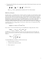
The RMS value of a function is defined as the square root of the average value (mean) of the square of a
function. If a function v(t) is periodic with a period of T, then the RMS of this function is mathematically
defined as:
To obtain the RMS value of a function, we follow these three steps:
1. Square the function over a period
2.
Calculate the mean of this new function
3. Take the square root
2
Example
Assume we have a triangular function with a
period of T =4 and an amplitude of A with no
DC offset. Because of symmetry, it suffices to
integrate v 2, from 0 to 1, i.e., to average over a
quarter period, to find the RMS value:
At
(A t)
2
The RMS of sine waveforms can be obtained similarly as done in the pre-lab.
Experimental procedure:
Note: throughout this experiment, set the FG to “High Z” output termination Impedance
a) Configure and store the following waveforms in the FG. You should be able to figure out how to store
waveforms (up to a maximum of three) in the Agilent 54621A oscilloscope, otherwise you can find out how
by checking its user’s manual (also available on line).
1) 6.00 Vpp sine wave @ 500 Hz with no DC offset
2) 2.12 Vrms sine wave @ 500Hz with no DC offset
3) 2.00 Vrms sine wave @ 1k Hz with 2.0 V DC offset
Note: for each waveform, enter its parameters into the function generator exactly as stated. In particular, this
will require you to switch back-and-forth between V peak-to-peak and V RMS (by pressing Enter Number,
then either ∧ or ∧).
b) Recall each of the three stored waveforms one at a time and perform the following measurements:
1) AC (Peak-to-Peak)
2) DC (Average)
3) RMS values
Perform these measurements on the oscilloscope only. To do so, press Quick Measure button, then Select and
Measure each of the following: AC (Peak-to-Peak), DC (Average), and RMS. For example, here is the results
that were obtained for the first waveform:
3
(Note how, as indicated by the dashed lines, the scope automatically performs the calculations over an
integer number of periods of the periodic waveform.) Always be sure the vertical sensitivity of the scope
is set so the waveform is not clipped; otherwise, it might perform the calculations incorrectly.
c) Repeat steps a and b for the following three waveforms
4) 2.00 Vrms sine wave @ 1k Hz with –2.0 V DC offset
5) 5.00 Vpp triangle wave @ 2K Hz with no DC offset
6) 6.00 Vpp square wave @ 2K Hz with no DC offset
d) Repeat steps, a and b for this waveform
7) 6.00 Vpp square wave @ 2K Hz with 1.0V DC offset
e) Display the results (AC, DC, and RMS values) in tabular form for all seven waveforms.
Questions: Section 1
1) How closely do waveforms 1 and 2 match each other for the AC reading? Why is that?
2) What would you mathematically expect waveform numbers 3, 4, and 5 to be for RMS values? How close are
these predictions to the actual scope readings?
3) How closely do the measurements for waveforms 6 and 7 match what was calculated in question 3 and 4 of
the prelab?
Section 2) Voltage Measurements at Various Frequencies
a) Configure the FG to supply a 3.0 Vrms sine wave @ 1 Hz with no DC offset.
b) Using the AC scale on the Agilent 34401A multimeter, measure the voltage output of the FG. You should
observe that at this very low frequency, the multimeter display jumps around!
c) Repeat steps a) and b) for the following frequencies: 10 Hz, 100 Hz, 1 kHz , … , 10 M Hz. Calculate the %
difference from the original 3.0 Vrms. Put the results in tabular form.
4
Question: Section 2
What trend is evident in the percent error?
Section 3) Function Generator/Counter Accuracy
a) Configure the FG to supply a 3.0 Vrms sine wave @ 500 Hz with 0V DC offset.
b) Use the Agilent 34401A Counter to measure this frequency and record the results.
c) Repeat steps a) and b) for the following frequencies: 10 Hz, 100 Hz, 1 kHz , … , 10 M Hz. Calculate the %
difference from the original 3.0 Vrms. Put the results in tabular form.
Questions: Section 3
What trend is evident in the percent error?
Section 4) Period Measurement with the Frequency Counter
a) Configure the FG to supply a 3.0 Vrms sine wave @ 1 Hz with no DC offset. Try to measure the period of this
waveform using the counter. Again, as in section 2 (a), you should observe that the multimeter display jumps
around at this very low frequency (<2 Hz).
b) Configure the FG to supply a 3.0 Vrms sinewave @ 100 Hz.
c) Measure and record the period of this waveform using the counter.
d) Repeat steps a) and b) for frequencies of 10 Hz, 100 Hz, 1 kHz , … , 10 M Hz. Calculate the % difference
from the original 3.0 Vrms. Put the results in tabular form.
Questions: Section 4
What trend is evident in the percent error?
Section 5) Analysis of the Measurement Error
In this section, we learn to analyze the measurement error.
Overview of Error Analysis
Data collection and interpretation is key to successful laboratory experimentation. There are two main types of
experimental errors in physical measurements.
Systematic Errors will cause the entire distribution of data points to be offset with respect to the true
value. Causes of systematic error include poor measurement technique, errors in instrumental calibration,
software errors or failure to correct for external conditions (e.g. temperature). Possible sources of
systematic error must be considered in all of the stages of the experiment, from design to data analysis.
Random Error is the deviation from the true value which occurs in any physical measurement. The
assumption is that this error will result in experimental readings which are equally distributed between
"too high" and "too low," and the mean value reflects the true average value, to within some precision.
5
Analysis of Random Error
Suppose you want to measure a physical property, e.g., the RMS value of a waveform. The numerical values that
the physical quantity can assume may be represented by a random variable R whose population is the set {X1 , X2
, X3,…, Xn }. Each Xi represents a possible value or outcome. Note that the population of R may include multiple
occurrences of the same value. Two important statistical properties of this set are the average value (mean) and
the standard deviation (standard error) defined as:
Average (mean):
Standard deviation (standard error):
The Standard Deviation (also known as Standard Error) measures the spread of the data about the mean value. It
represents the expected error in a single measurement of a physical quantity, i.e., the expected deviation from its
true mean. In laboratory measurements, we can only obtain a subset of the entire population (i.e., all possible
outcomes of a measurement) of R. For this reason, we can only obtain estimates of the true average and standard
error. If a measurement is carried out m times, where m < n, then we can use the above equations to estimate the
average and standard error by replacing n with m. This means that more measurements translate to smaller errors
in the estimate of the true mean and standard error. Note that the measurements are assumed to be unbiased and
carried out under identical conditions.
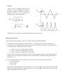
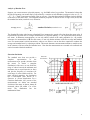
Gaussian distribution
The standard error does not provide a
complete
representation
of
the
measurement error spread (deviation from
the mean). To obtain a complete
distribution of the error, we can divide the
range of values between the minimum and
maximum into m equal intervals (or bins)
and plot the frequency of occurrence for
each range of values within each bin. For
many physical quantities, the distribution
has a bell-shaped form known as a
Gaussian or normal distribution. For a
Gaussian distribution, 68.3 percent of the
measurements are within one standard
deviation of the mean. As shown, almost all
measured values fall within ±3σ of the
mean.
The
distribution
has
the
mathematical form:
Gaussian
distribution
3σ
Measurement intervals (bins)
6
Experimental Procedure
Note:
An executable program “The Gaussian Calculator” has
been designed in order to assist in the construction of
Gaussian distribution plots required in parts (e) through
(g). This is done by categorizing entered values into
specific bins of a predetermined size. Once all the
values have been entered, the data is exportable to any
spreadsheet applications. The Gaussian Calculator is
also useful in quickly calculating the average value and
standard deviation. The executable code and the user
guide are available either from the EE 241 directory or
by clicking the following links:
Gaussian Calculator User Guide:
Gaussian Calculator Executable:
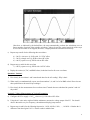
The Gaussian Calculator application
a)
Configure and store the following waveforms in the Agilent function generator
Vpp sine wave @ 1 KHz with no DC offset
b)
Connect the FG output to the Agilent oscilloscope (for this experiment, you can use a black coaxial BNC
to BNC cable)
c)
Set the scope to AC coupled and press the “Quick/Meas” button on the scope panel and then select RMS
measurement. You will notice that the digital readout (for the RMS value of the waveform) of the scope
is not stable; the least significant digit is constantly changing. The continually changing readout can be
assumed to represent the varying outcomes (values) of a measurement process (RMS value of the FG
output waveform).
d)
Freeze the waveform by pressing the “Stop/Run” button on the scope panel (thereby making it turn red)
to read and record the digital readout at any moment. Once the Sop/Run button of the scope has been
pressed, successive individual traces can be obtained by pressing the Single button. Obtain 10 RMS
readings and record them in a table.
e)
Calculate the mean and the standard deviation for the set of ten measurements.
f)
Increase the number of readings to 20 and recalculate the mean and standard deviation. Record the
differences from the previous values in your table.
g)
Increase the number of measurements to 40 and plot the distribution of the error (deviation from the
mean).
7
h)
Manually fit the above standard error distribution to a Gaussian distribution function as shown in the
figure above. Estimate the standard deviation from the manually fitted Gaussian curve (Remember the
curve spans ±3σ about the mean) and record the percent difference from the calculated value.
Questions: section 5
1) How and why do the estimates of the mean and standard deviation change as we increased the number of
samples from 10 to 20?
2) How close is the mean value (based on the 20-point sample set) to the theoretical value? If we increase
the number of measurements to say 1000, will we nearly reach the theoretical value?
3) For error analysis, would it be acceptable if you obtain additional measurement values from students on
other benches?
4) What change do you expect in the difference between the calculated and manually measured values of the
standard error as the number of measurements increase? (explain).
5)
Do you expect the error distribution look more “normal” as the number of measurements increase?
8