Download SExtractor User`s Guide

Dr
SExtractor
v2.5
User’s manual
E. BERTIN
Institut d’Astrophysique
& Observatoire de Paris
1
aft
2
Contents
1 What is SExtractor?
5
2 Installing the software
5
2.1
Software and hardware requirements . . . . . . . . . . . . . . . . . . . . . . . . .
5
2.2
Obtaining SExtractor . . . . . . . . . . . . . . . . . . . . . . . . . . . . . . . .
6
2.3
Installation . . . . . . . . . . . . . . . . . . . . . . . . . . . . . . . . . . . . . . .
6
3 Using SExtractor
6
3.1
Syntax . . . . . . . . . . . . . . . . . . . . . . . . . . . . . . . . . . . . . . . . . .
6
3.2
The configuration file . . . . . . . . . . . . . . . . . . . . . . . . . . . . . . . . . .
6
3.2.1
Format . . . . . . . . . . . . . . . . . . . . . . . . . . . . . . . . . . . . .
7
3.2.2
Configuration parameter list
. . . . . . . . . . . . . . . . . . . . . . . . .
7
The catalog parameter file . . . . . . . . . . . . . . . . . . . . . . . . . . . . . . .
12
3.3.1
Format . . . . . . . . . . . . . . . . . . . . . . . . . . . . . . . . . . . . .
12
Example of configuration . . . . . . . . . . . . . . . . . . . . . . . . . . . . . . .
12
3.3
3.4
4 Overview of the software
12
5 Handling of image data
12
6 Detection and segmentation
14
6.1
6.2
6.3
6.4
Background estimation . . . . . . . . . . . . . . . . . . . . . . . . . . . . . . . . .
14
6.1.1
Configuration parameters and tuning . . . . . . . . . . . . . . . . . . . . .
16
6.1.2
CPU cost . . . . . . . . . . . . . . . . . . . . . . . . . . . . . . . . . . . .
16
Filtering . . . . . . . . . . . . . . . . . . . . . . . . . . . . . . . . . . . . . . . . .
16
6.2.1
Convolution . . . . . . . . . . . . . . . . . . . . . . . . . . . . . . . . . . .
16
6.2.2
Non-linear filtering . . . . . . . . . . . . . . . . . . . . . . . . . . . . . . .
18
6.2.3
What is filtered, and what isn’t . . . . . . . . . . . . . . . . . . . . . . . .
18
6.2.4
Image boundaries and bad pixels . . . . . . . . . . . . . . . . . . . . . . .
18
6.2.5
Configuration parameters. . . . . . . . . . . . . . . . . . . . . . . . . . . .
18
6.2.6
CPU cost. . . . . . . . . . . . . . . . . . . . . . . . . . . . . . . . . . . . .
19
6.2.7
Filter file formats. . . . . . . . . . . . . . . . . . . . . . . . . . . . . . . .
19
Thresholding . . . . . . . . . . . . . . . . . . . . . . . . . . . . . . . . . . . . . .
20
6.3.1
Configuration parameters. . . . . . . . . . . . . . . . . . . . . . . . . . . .
20
Deblending . . . . . . . . . . . . . . . . . . . . . . . . . . . . . . . . . . . . . . .
20
3
7 Weighting
23
7.1
Weight-map formats . . . . . . . . . . . . . . . . . . . . . . . . . . . . . . . . . .
23
7.2
Weight threshold . . . . . . . . . . . . . . . . . . . . . . . . . . . . . . . . . . . .
24
7.3
Effect of weighting . . . . . . . . . . . . . . . . . . . . . . . . . . . . . . . . . . .
24
7.4
Combining weight maps . . . . . . . . . . . . . . . . . . . . . . . . . . . . . . . .
25
7.5
Interpolation . . . . . . . . . . . . . . . . . . . . . . . . . . . . . . . . . . . . . .
25
8 Flags
25
8.1
Internal flags . . . . . . . . . . . . . . . . . . . . . . . . . . . . . . . . . . . . . .
25
8.2
External flags . . . . . . . . . . . . . . . . . . . . . . . . . . . . . . . . . . . . . .
26
9 Measurements
9.1
26
Positional parameters derived from the isophotal profile . . . . . . . . . . . . . .
27
9.1.1
Limits: XMIN, YMIN, XMAX, YMAX . . . . . . . . . . . . . . . . . . . . . . . .
27
9.1.2
Barycenter: X, Y . . . . . . . . . . . . . . . . . . . . . . . . . . . . . . . .
27
9.1.3
Position of the peak: XPEAK, YPEAK . . . . . . . . . . . . . . . . . . . . . .
27
9.1.4
2nd order moments: X2, Y2, XY . . . . . . . . . . . . . . . . . . . . . . . .
28
9.1.5
Basic shape parameters: A, B, THETA . . . . . . . . . . . . . . . . . . . . .
28
9.1.6
Ellipse parameters: CXX, CYY, CXY . . . . . . . . . . . . . . . . . . . . . . .
29
9.1.7
By-products of shape parameters: ELONGATION, ELLIPTICITY . . . . . . .
30
9.1.8
Position errors: ERRX2, ERRY2, ERRXY, ERRA, ERRB, ERRTHETA, ERRCXX,
ERRCYY, ERRCXY . . . . . . . . . . . . . . . . . . . . . . . . . . . . . . . . .
30
Handling of “infinitely thin” detections
. . . . . . . . . . . . . . . . . . .
31
9.2
Windowed positional parameters . . . . . . . . . . . . . . . . . . . . . . . . . . .
32
9.3
Astrometry and WORLD coordinates . . . . . . . . . . . . . . . . . . . . . . . . . .
32
9.3.1
Celestial coordinates . . . . . . . . . . . . . . . . . . . . . . . . . . . . . .
33
9.3.2
Use of the FITS keywords for astrometry . . . . . . . . . . . . . . . . . .
34
9.4
Photometry . . . . . . . . . . . . . . . . . . . . . . . . . . . . . . . . . . . . . . .
34
9.5
Cross-identification within SExtractor . . . . . . . . . . . . . . . . . . . . . .
37
9.5.1
The ASSOC list . . . . . . . . . . . . . . . . . . . . . . . . . . . . . . . . .
37
9.5.2
Controlling the ASSOC process . . . . . . . . . . . . . . . . . . . . . . . . .
37
9.5.3
Output from ASSOC . . . . . . . . . . . . . . . . . . . . . . . . . . . . . . .
38
9.1.9
A Appendices
39
A.1 FAQ (Frequently Asked Questions) . . . . . . . . . . . . . . . . . . . . . . . . . .
4
39
1
What is SExtractor?
SExtractor (Source-Extractor) is a program that builds a catalogue of objects from an astronomical image. It is particularly oriented towards reduction of large scale galaxy-survey data,
but it also performs well on moderately crowded star fields. Its main features are:
• Support for multi-extension FITS.
• Speed: typically 1 Mpixel/s with a 2GHz processor.
• Ability to work with very large images (up to 65k × 65k pixels on 32 bit machines, or
2G × 2G pixels on 64 bit machines), thanks to buffered image access.
• Robust deblending of overlapping extended objects.
• Real-time filtering of images to improve detectability.
• Neural-Network-based star/galaxy classifier.
• Flexible catalogue output of desired parameters only.
• Pixel-to-pixel photometry in dual-image mode.
• Handling of weight-maps and flag-maps.
• Optimum handling of images with variable S/N.
• Special mode for photographic scans.
• XML VOTable-compliant catalog output.
Back in the early nineties, the purpose of SExtractor was to find a compromise between refinement in both detection and measurements, and computational speed. By today’s standards,
SExtractor would be more accurately described as a “quick-and-dirty” tool.
2
Installing the software
2.1
Software and hardware requirements
Since the beginning in 1993, the development of SExtractor was always made on Unix systems
(successively: SUN-OS, HP/UX, SUN-Solaris, Digital Unix and GNU/Linux). Successful ports
by external contributors have been reported on non-Unix OSes such as AMIGA-OS, DEC-VMS
and even MS-DOS Windows951 and NT ; ). They are however not currently supported by the
author, and Unix remains the recommended system for running SExtractor. The software
is generally run in (ANSI) text-mode from a shell. A window system is therefore unnecessary
with present versions.
On the hardware side, memory requirements obviously depend on the size of the images to be
processed. But to give an idea, a typical processing of 1024×1024 pixel images should require no
more than 8 MB of memory. For very large images, (32000 × 32000 pixels or more), a minimum
of 200MB is recommended. Swap-space can of course be put to contribution, although a strong
performance hit is to be expected.
1
Binaries are available on the WWW, see e.g. http://www.tass-survey.org/tass/software/software.html#sextract
5
2.2
Obtaining SExtractor
The easiest way to obtain SExtractor is to download it from http://terapix.iap.fr/soft/sextractor/.
The current official anonymous FTP site is ftp://ftp.iap.fr/pub/from users/bertin/sextractor/.
There can be found the latest versions of the program as standard .tar.gz Unix archives, plus
some documentation.
2.3
Installation
To install from the source archive, you must first uncompress and unarchive the archive:
gzip -dc sextractor-x.y.tar.gz | tar xv
A new directory called sextractor-x.y should now appear at the current position on your disk.
You should then just enter the directory and follow the instructions in the file called “INSTALL”.
If you have the root privileges, it will generally consist of
% ./configure
% make
% make install
RPM binary archives are also provided for x86 architectures (e.g. Intel, AMD). In this case,
SExtractor can be installed as root using
% rpm -U sextractor-x.y.-z.rpm
3
3.1
Using SExtractor
Syntax
SExtractor is run from the shell with the following syntax:
% sex image [-c configuration-file] [ -Parameter1 Value1 ] [ -Parameter2 Value2 ] ...
The part enclosed within brackets is optional. Any ”-Parameter Value” statement in the
command-line overrides the corresponding definition in the configuration-file or any default
value (see below). Actually, two image filenames can be provided, separated by a comma:
%
sex image1,image2
This syntax makes SExtractor run in the so-called “double-image mode”: image1 will be
used for detection of sources, and image2 for measurements only. image1 and image2 must
have the same dimensions. Changing image2 for another image will not modify the number of
detected sources, neither affect their positional or basic shape parameters. But most photometric
parameters, plus a few others, will use image2 pixel values, which allows one to easily measure
pixel-to-pixel colours.
3.2
The configuration file
SExtractor needs several files for its configuration. If no configuration file-name is specified
in the command line, SExtractor tries to load a file called “default.sex” from the local
directory. If default.sex is not found, it loads default values defined internally. The default
6
parameters can be listed with the command
%
sex -d
3.2.1
Format
The format is ASCII. There must be only one parameter set per line, following the form:
Config-parameter
Value(s)
Extra spaces or linefeeds are ignored. Comments must begin with a “#” and end with a linefeed.
Values can be of different types: strings (can be enclosed between double quotes), floats, integers,
keywords or boolean (Y/y or N/n). Some parameters accept zero or several values, which must
then be separated by commas. Integers can be given as decimals, in octal form (preceded by digit
O), or in hexadecimal (preceded by 0x). The hexadecimal format is particularly convenient for
writing multiplexed bit values such as binary masks. Environment variables, written as $HOME
or ${HOME} are expanded, and not only for string parameters. Some parameters are assigned
default values in SExtractor and can therefore be omitted from the configuration file; they
are listed in §3.2.2.
3.2.2
Configuration parameter list
Here is a complete list of all the configuration parameters known to SExtractor. Many of
them should be used with their default values. Please refer to the next sections for a detailed
description of their meaning.
Parameter
ANALYSIS THRESH
default
—
type
floats (n ≤ 2)
ASSOC DATA
2,3,4
integers (n ≤ 32)
ASSOC NAME
ASSOC PARAMS
sky.list
2,3,4
string
integers (2 ≤ n ≤ 3)
ASSOC RADIUS
ASSOC TYPE
2.0
MAG SUM
float
keyword
FIRST
NEAREST
MEAN
MAG MEAN
SUM
MAG SUM
MIN
7
Description
Threshold (in surface brightness) at
which CLASS STAR and FWHM operate.
1 argument: relative to
Background RMS. 2 arguments: mu
(mag.arcsec−2 ), Zero-point (mag).
# of the columns in the ASSOC file that
will be copied to the catalog output.
Name of the ASSOC ASCII file.
Nos of the columns in the ASSOC file
that will be used as coordinates and
weight for cross-matching.
Search radius (in pixels) for ASSOC.
Method for cross-matching in ASSOC:
– keep values corresponding to the
first match found,
– values corresponding to the nearest
match found,
– weighted-average values,
– exponentialy weighted-average values,
– sum values,
– exponentialy sum values,
– keep values corresponding to the
match with minimum weight,
MAX
ASSOCSELEC TYPE
MATCHED
keyword
ALL
MATCHED
-MATCHED
BACK FILTERSIZE
—
integers (n ≤ 2)
BACK SIZE
—
integers (n ≤ 2)
BACK TYPE
AUTO
keywords (n ≤ 2)
AUTO
MANUAL
BACK VALUE
0.0,0.0
floats (n ≤ 2)
BACKPHOTO THICK
24
integer
BACKPHOTO TYPE
GLOBAL
keyword
GLOBAL
LOCAL
CATALOG NAME
—
string
CATALOG TYPE
—
keyword
ASCII
ASCII HEAD
ASCII SKYCAT
ASCII VOTABLE
FITS 1.0
FITS LDAC
CHECKIMAGE NAME
check.fits
strings (n ≤ 16)
8
– keep values corresponding to the
match with maximum weight.
What sources are printed in the output catalog in case of ASSOC:
– all detections,
– only matched detections,
– only detections that were not
matched.
Size, or Width,Height (in background
meshes) of the background-filtering
mask.
Size, or Width,Height (in pixels) of a
background mesh.
What background is subtracted from
the images:
– the internal, automatically interpolated background-map,
– a user-supplied constant value provided in BACK VALUE.
in BACK TYPE MANUAL mode, the constant value to be subtracted from the
images.
Thickness (in pixels) of the background LOCAL annulus.
Background used to compute magnitudes:
– taken directly from the background
map,
– recomputed in a “rectangular annulus” around the object.
Name of the output catalogue. If
the name “STDOUT” is given and
CATALOG TYPE is set to ASCII,
ASCII SKYCAT,
or
ASCII HEAD,
ASCII VOTABLE the catalogue will be
piped to the standard output (stdout)
Format of output catalog:
– ASCII table; the simplest, but space
and time consuming,
– as ASCII, preceded by a header containing information about the content,
– SkyCat ASCII format (WCS coordinates required),
– XML-VOTable format, together
with meta-data,
– FITS format as in SExtractor 1,
– FITS “LDAC” format (the original
image header is copied).
File name for each “check-image”.
CHECKIMAGE TYPE
NONE
keywords (n ≤ 16)
NONE
IDENTICAL
BACKGROUND
BACKGROUND RMS
MINIBACKGROUND
MINIBACK RMS
-BACKGROUND
FILTERED
OBJECTS
-OBJECTS
APERTURES
SEGMENTATION
CLEAN
—
boolean
CLEAN PARAM
DEBLEND MINCONT
—
—
float
float
DEBLEND NTHRESH
DETECT MINAREA
—
—
integer
integer
DETECT THRESH
—
floats (n ≤ 2)
DETECT TYPE
CCD
keyword
CCD
FILTER
—
PHOTO
boolean
FILTER NAME
—
string
floats (n ≤ 2)
FILTER THRESH
FITS UNSIGNED
N
boolean
FLAG IMAGE
flag.fits
strings (n ≤ 4)
9
Type of information to put in the
“check-images”:
– no check-image,
– identical to input image (useful for
converting formats),
– full-resolution interpolated background map,
– full-resolution interpolated background noise map,
– low-resolution background map,
– low-resolution background noise
map,
– background-subtracted image,
– background-subtracted filtered image (requires FILTER = Y),
– detected objects,
– background-subtracted image with
detected objects blanked,
– MAG APER and MAG AUTO integration
limits,
– display patches corresponding to
pixels attributed to each object.
If true, a “cleaning” of the catalogue
is done before being written to disk.
Efficiency of “cleaning”.
Minimum contrast parameter for deblending.
Number of deblending sub-thresholds.
Minimum number of pixels above
threshold triggering detection.
Detection threshold.
1 argument:
(ADUs or relative to Background
RMS, see THRESH TYPE). 2 arguments:
µ (mag.arcsec−2 ), Zero-point (mag).
Type of device that produced the image:
– linear detector like CCDs or NICMOS,
– photographic scan.
If true, filtering is applied to the data
before extraction.
Name of the file containing the filter
definition.
Lower and higher thresholds (in background standard deviations) for a
pixel to be considered in filtering (used
for retina-filtering only).
Force 16-bit FITS input data to be interpreted as unsigned integers.
File name(s) of the “flag-image(s)”.
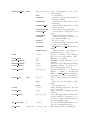
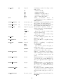
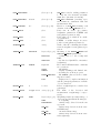
FLAG TYPE
OR
keyword
OR
AND
MIN
MAX
MOST
float
GAIN
INTERP MAXXLAG
16
integers (n ≤ 2)
INTERP MAXYLAG
16
integers (n ≤ 2)
INTERP TYPE
ALL
keywords (n ≤ 2)
NONE
VAR ONLY
ALL
MAG GAMMA
float
MAG ZEROPOINT
float
MASK TYPE
CORRECT
keyword
NONE
BLANK
CORRECT
MEMORY BUFSIZE
—
integer
MEMORY OBJSTACK
—
integer
MEMORY PIXSTACK
—
integer
PARAMETERS NAME
—
string
PHOT APERTURES
—
floats (n ≤ 32)
10
Combination method for flags on the
same object:
– arithmetical OR,
– arithmetical AND,
– minimum of all flag values,
– maximum of all flag values,
– most common flag value.
“Gain”
(conversion
factor
in
e− /ADU) used for error estimates of
CCD magnitudes .
Maximum x gap (in pixels) allowed in
interpolating the input image(s).
Maximum y gap (in pixels) allowed in
interpolating the input image(s).
Interpolation method from the
variance-map(s) (or weight-map(s)):
– no interpolation,
– interpolate only the variance-map
(detection threshold),
– interpolate both the variance-map
and the image itself.
γ of the emulsion (takes effect in
PHOTO mode only).
Zero-point offset to be applied to magnitudes.
Method of “masking” of neighbours
for photometry:
– no masking,
– put detected pixels belonging to
neighbours to zero,
– replace by values of pixels symetric
with respect to the source center.
Number of scan-lines in the imagebuffer. Multiply by 4 the frame width
to get equivalent memory space in
bytes.
Maximum number of objects that the
object-stack can contain. Multiply by
300 to get equivalent memory space in
bytes.
Maximum number of pixels that the
pixel-stack can contain. Multiply by
16 to 32 to get equivalent memory
space in bytes.
The name of the file containing the list
of parameters that will be computed
and put in the catalogue for each object.
Aperture diameters in pixels (used by
MAG APER).
PHOT AUTOPARAMS
—
floats (n = 2)
PHOT AUTOAPERS
0.0,0.0
floats (n = 2)
PHOT FLUXFRAC
0.5
floats (n ≤ 32)
PIXEL SCALE
—
float
SATUR LEVEL
—
float
SEEING FWHM
—
float
STARNNW NAME
—
string
THRESH TYPE
RELATIVE
keywords (n ≤ 2)
RELATIVE
ABSOLUTE
VERBOSE TYPE
NORMAL
keyword
QUIET
NORMAL
EXTRA WARNINGS
FULL
WEIGHT GAIN
Y
boolean
WEIGHT IMAGE
weight.fits
strings (n ≤ 2)
WEIGHT TYPE
NONE
keywords (n ≤ 2)
NONE
BACKGROUND
MAP RMS
MAP VAR
MAP WEIGHT
11
MAG AUTO controls: scaling parameter
k of the 1st order moment, and minimum Rmin (in units of A and B).
MAG AUTO minimum (circular) aperture diameters: estimation disk, and
measurement disk.
Fraction of FLUX AUTO defining each
element of the FLUX RADIUS vector.
Pixel size in arcsec (for surface
brightness parameters, FWHM and
star/galaxy separation only).
Pixel value above which it is considered saturated.
FWHM of stellar images in arcsec
(only for star/galaxy separation).
Name of the file containing the neuralnetwork weights for star/galaxy separation.
Meaning of the DETECT THRESH and
ANALYSIS THRESH parameters :
– scaling factor to the background
RMS,
– absolute level (in ADUs or in surface
brightness).
How much SExtractor comments
its operations:
– run silently,
– display warnings and limited info
concerning the work in progress,
– like NORMAL, plus a few more warnings if necessary,
– display a more complete information
and the principal parameters of all the
objects extracted.
If true, weight maps are considered as
gain maps.
File name of the detection and
measurement “weight-image”, respectively.
Weighting scheme (for single image, or
detection and measurement images):
– no weighting,
– variance-map derived from the image itself,
– variance-map derived from an external RMS-map,
– external variance-map,
– variance-map derived from an external weight-map,
WRITE XML
N
boolean
XML NAME
sex.xml
string
3.3
If true, meta-data will be written in
XML-VOTable format.
File name for the XML output of
SExtractor.
The catalog parameter file
In addition to the configuration file detailed above, SExtractor needs a file containing the list
of parameters that will be listed in the output catalog for every detection. This allows the software to compute only catalog parameters that are needed. The name of this catalog-parameter
file is traditionally suffixed with .param, and must be specified using the PARAMETERS NAME
config parameter.
3.3.1
Format
The format of the catalog parameter list is ASCII, and there must be only one keyword per
line. Presently two kinds of keywords are recognized by SExtractor: scalars and vectors.
Scalars, like X IMAGE, yield single numbers in the output catalog. Vectors, like MAG APER(4) or
VIGNET(15,15), yield arrays of numbers. The order in which the parameters will be listed in
the catalogue are the same as that of the keywords in the parameter list. Comments are allowed,
they must begin with a “#”. Here is a descriptive list of available parameter keywords.
3.4
4
Example of configuration
Overview of the software
The complete analysis of an image is done in two passes through the data. During the first
pass, a model of the sky background is built, and a couple of global statistics are estimated.
During the second pass, the image is background-subtracted, filtered and thresholded “on-thefly”. Detections are then deblended, pruned (“CLEANed”), photometered, classified and finally
written to the output catalog. The following sections enter a little more into the details of each
of these operations2 .
5
Handling of image data
SExtractor accepts images stored in FITS3 format (Wells et al. 1981, see also http://fits.gsfc.nasa.gov).
Both “Basic FITS” (one single header and one single body) and “Multi-Extension-FITS” (MEF)
images are recognized. Binary SExtractor catalogs produced from MEF images are MEF files
themselves. If catalog output is in ASCII format, all catalogs from the individual extensions
are concatenated in one big file; the EXT NUMBER catalog parameter must be used to tell which
extension the source belongs to.
For images with NAXIS > 2, only the first data-plane is loaded. If WCS4 information (Greisen
1
Optional parameter
In the text, uppercase keywords in typewriter font refer to parameters from the configuration file or from the
parameter file
3
Flexible Image Transport System
4
World Coordinate System
2
12
Input frame
Frame buffer
Background
subtraction
Weight-map
Frame buffer
Image
filtering
Convolution
mask,
or Retina
Image
segmentation
Flag-map
Frame buffer
De-blending
Pixelstack
Ext. weight map
Isophotal
analysis
‘‘Cleaning’’
of detections
Frame buffer
External image
Objectstack
Frame buffer
PSF mapping
Photometry
Astrometry
Background
subtraction
Input catalog
(ASCII)
Crossidentification
Output catalog
Figure 1: Layout of the main SExtractor procedures. Dashed arrows represent optional
inputs.
13
& Calabretta 1995, http://www.cv.nrao.edu/fits/documents/wcs/wcs.all.ps) is available
in the header, it is automatically used by SExtractor to compute astrometric parameters.
Other astrometric descriptions like AST (Starlink format) or the solution coefficients of the DSS
5 plates are not recognized by the software.
In SExtractor, as in all similar programs, FITS axis “1” is traditionaly refered as the X axis,
and FITS axis “2” as the Y axis.
6
Detection and segmentation
In SExtractor, the detection of sources is part of a process called segmentation in the imageprocessing vocabulary. Segmentation normally consists of identifying and separating image
regions which have different properties (brightness, colour, texture...) or are delineated by
edges. In the astronomical context, the segmentation process consists of separating objects from
the sky background. This is however a somewhat imprecise definition, as astronomical sources
have, on the images — and even often physically —, no clear boundaries, and may overlap.
We shall therefore use the following working definition of an object in SExtractor: a group
of pixels selected through some detection process and for which the flux contribution of an
astronomical source is believed to be dominant over that of other objects. Note that this means
that a simple x, y position vector alone cannot be handled by SExtractor as a detection: most
measurement routines require some rough shape information about the objects.
Segmentation in SExtractor is achieved through a very simple thresholding process: a group
of connected pixels that exceed some threshold above the background is identified as a detection.
But things are a little bit more complicated in practice. First, on most astronomical images, the
background is not constant over the frame, and its determination can be ambiguous in crowded
regions. Second, the software has to operate on noisy data, and some filtering adapted to the
characteristics of the image has to be applied prior to detection, to reduce the contamination by
noise peaks. Third, many sources that overlap on the image are unlikely to be detected separately
with a single detection threshold, and require a de-blending procedure, which is actually multithresholding in SExtractor. Each of these points will now be described in greater detail
below. It is worth mentioning here that these 3 difficulties could, to a large extent, be bypassed
using a wavelet decomposition (e.g. Bijaoui et al. 1998). Although such an algorithm might
be implemented in a future version of SExtractor, current constraints in processing speed,
available memory (processing of gigantic images) often make the “pedestrian approach” still
more interesting in the case of large scale surveys.
6.1
Background estimation
The value measured at each pixel is a function of the sum of a “background” signal and light
coming from the objects of interest. To be able to detect the faintest of these objects and also
to measure accurately their fluxes, one needs to have an accurate estimate of the background
level in any place of the image, a “background map”. Strictly speaking, there should be one
background map per object, that is, what would the image look like if that object was absent.
But, at least for detection, we may start by assuming that most discrete sources do not overlap
too severely, which is generally the case for high galactic latitude fields.
To construct the background map, SExtractor makes a first pass through the pixel data,
computing an estimator for the local background in each mesh of a grid that covers the whole
5
Digital Sky Survey
14
frame. The background estimator is a combination of κ.σ clipping and mode estimation, similar
to the one employed in Stetson’s DAOPHOT program (see e.g. Da Costa 1992). Briefly, the
local background histogram is clipped iteratively until convergence at ±3σ around its median;
if σ is changed by less than 20% during that process, we consider that the field is not crowded
and we simply take the mean of the clipped histogram as a value for the background; otherwise
we estimate the mode with:
Mode = 2.5 × Median − 1.5 × Mean
(1)
This expression is different from the usual approximation
Mode = 3 × Median − 2 × Mean
(2)
(e.g. Kendall and Stuart 1977), but was found to be more accurate with our clipped distributions, from the simulations we made. Fig. 2 shows that the expression of the mode above
is considerably less affected6 by crowding than a simple clipped mean — like the one used in
FOCAS (Jarvis and Tyson 1981) or by Infante (1987) — but is ≈ 30% noisier. For this reason
we revert to the mean in non-crowded fields.
10
Clipped Mode (ADU)
5
0
-5
-10
0
5
10
15
Clipped Mean (ADU)
20
25
30
Figure 2: Simulations of 32×32 pixels background meshes polluted by random Gaussian profiles.
The true background lies at 0 ADU. While being slightly noisier, the clipped “Mode” gives a
more robust estimate than a clipped Mean in crowded regions.
Once the grid is set up, a median filter can be applied to suppress possible local overestimations
due to bright stars. The resulting background map is then simply a (natural) bicubic-spline
interpolation between the meshes of the grid. In parallel with the making of the background map,
an “RMS-background-map”, that is, a map of the background noise in the image is produced.
It will be used if the WEIGHT TYPE parameter is set different from NONE (see §7.1).
6
Obviously in some very unfavorable cases (like small meshes falling on bright stars), it leads to totally
inaccurate results.
15
6.1.1
Configuration parameters and tuning
. The choice of the mesh size (BACK SIZE) is very important. If it is too small, the background
estimation is affected by the presence of objects and random noise. Most importantly, part of
the flux of the most extended objects can be absorbed in the background map. If the mesh size
is too large, it cannot reproduce the small scale variations of the background. Therefore a good
compromise has to be found by the user. Typically, for reasonably sampled images, a width7 of
32 to 256 pixels works well. The user has some control over the background map by specifying
the size of the median filter (BACK FILTERSIZE). A width and height of 1 means that no filtering
will be applied to the background grid. Usually a size of 3× 3 is enough, but it may be necessary
to use larger dimensions, especially to compensate, in part, for small background mesh sizes, or
in the case of large artefacts in the images. Median filtering also helps reducing possible ringing
effects of the bicubic-spline around bright features. In some specific cases it might be desirable
to median-filter only background meshes whose original values exceed some threshold above the
filtered-value. This differential threshold is set by the BACK FILTERTHRESH parameter, in ADUs.
It is important to note that all BACK configuration parameters also affect the background-RMS
map.
By default the computed background-map is automatically subtracted from the input image.
But there are some situations where it is more appropriate to subtract a constant from the
image (e.g., images where the background noise distribution is strongly skewed). The BACK TYPE
configuration parameter (set by default to “AUTO”) can be switched to MANUAL to allow for
the value specified by the BACK DEFAULT parameter to be subtracted from the input image. The
default value is 0.
6.1.2
CPU cost
. The background estimation operation can take a considerable time on the largest images, e.g.
a few minutes minutes for a 32000 × 32000 frame on a 2GHz processor.
6.2
6.2.1
Filtering
Convolution
Detectability is generally limited at the faintest flux levels by a background noise. The powerspectrum of the noise and that of the superimposed signal can be significantly different. Some
gain in the ability to detect sources may therefore be obtained simply through appropriate linear
filtering of the data, prior to segmentation. In low density fields, an optimal convolution kernel
h (“matched filter”) can be found that maximizes detectability. An estimator of detectability is
for instance the signal-to-noise ratio at source position (x0 , y 0 ) ≡ (0, 0):
S
N
2
((s ∗ h)(x0 , y 0 ))2
,
≡
(n ∗ h)2
(3)
where s is the signal to be detected, n the noise, and ‘∗’ the convolution operator. Moving to
Fourier space, we get:
R
2
S
( SH dω)2
,
(4)
=R
|N |2 |H|2 dω
N
7
SExtractor offers the possibility of rectangular background meshes; but it is advised to use square ones,
except in some very special cases (rapidly varying background in one direction for example).
16
where S and H are the Fourier-transforms of s and h, respectively, and |N |2 is the powerspectrum of the noise. Remarking, using Schwartz inequality, that
we see that
Z
2
Z
Z
|S|2
SH dω ≤
dω
|N |2 |H|2 dω ,
|N |2
2
(5)
|S|2
dω .
|N |2
(6)
S
∝ |N |H∗ , that is
|N |
(7)
S
N
Z
≤
Equality (maximum S/N) in (5) and (6) is achieved for
H∝
S∗
.
|N |2
(8)
In the case of white noise (a valid approximation for many astronomical images, especially CCD
ones), |N |2 = cste ; the optimal convolution kernel for detecting stars is then the PSF flipped
over the x and y directions. It may also be described as the cross-correlation with the template
of the sources to be detected (for more details see, e.g. Bijaoui & Dantel 1970, or Das 1991).
There are of course a few problems with this method. First of all, many sources of unquestionable
interest, like galaxies, appear in a variety of shapes and scales on astronomical images. A
perfectly optimized detection routine should ultimately apply all relevant convolution kernels
one after the other in order to make a complete catalog. Approximations to this approach are the
(isotropic) wavelet analysis mentioned earlier, or the more empirical ImCat algorithm (Kaiser
et al. 1995), for both of which sources to detect are assumed to be reasonably round. The impact
on memory usage and processing speed of such refinements is currently judged too severe to be
applied in SExtractor. Simple filtering does a good job in general: the topological constraints
added by the segmentation process make the detection somewhat tolerant towards larger objects.
Extended, very Low-Surface-Brightness (LSB) features found in astronomical images are often
artifacts (flat-fielding errors, optical “ghosts” or halos). However, it is true that some of them
can be genuine objects, like LSB galaxies, or distant galaxy clusters burried in the background
noise. For detecting those with software like SExtractor, a specific processing is needed (see
for instance Dalcanton et al. 1997 and references therein). The simplest way to achieve the
detection of extended LSB objects in SExtractor is to work on MINIBACK check-images (see
§??).
A second problem may occur because of overlaps with other objects. Convolving with a lowpass filter (the PSF has no negative side-lobes) diminishes the contrast between objects, and
makes segmentation less effective in isolating individual sources. This can to some extent be
recovered by deblending (see §6.4). In severely crowded fields however, confusion noise becomes
the limiting factor for detection, and it is then advisable not to filter at all, or to use a bandpassfilter (compensated filter).
Finally, the PSF appears sometimes to be variable across the field. The convolution mask should
ideally follow these changes in order to allow for optimal detection everywhere in the image.
However, considering approximately-Gaussian PSF cores and convolution kernels, detectability
is a rather slow function of their FWHMs8 : a mismatch as large as 50% between the kernel
FWHM and that of the PSF will lead to no more than a 10% loss in peak S/N (Irwin 1985).
Considering that PSF variations are generally much smaller than this, filtering in SExtractor
is limited to constant kernels.
8
Full-Width at Half-Maximum
17
6.2.2
Non-linear filtering
There are many situations in which convolution is of little help: filtering of (strongly) nonGaussian noise, extraction of specific image patterns,... In those cases, one would like to extend
the concept of a convolution kernel to that of a more general stationnary filter, able for instance
to mimick boolean-like operations on pixels. What one wants like is thus a mapping from Rn
to R around each pixel. But the more general the filter, the more difficult it is to design “byhand” for each case, specifying how input pixel #i should be taken into account with respect
to input pixel #j to form the output, etc.. The solution to this is machine-learning. Given
a training set containing input and output pixels, a machine-learning software will adapt its
internal parameters in order to minimize a “cost function” (generally a χ2 error) and converge
toward the desired mapping-function. These parameters can then for example be reloaded by a
“read-only” routine to provide the actual filtering.
SExtractor implements this kind of “read-only” functionnality in the form of the so-called
“retina-filtering”. The EyE9 software (Bertin 1997) performs neural-network-learning on input
and output images to produce “retina-files”. These files contain weights that describe the
behaviour of the neural network. The neural network can thus be seen as an “artificial retina”
that takes its stimuli from a small rectangular array of pixels and produces a response according
to prior learning (for more details, see the EyE documentation). Typical applications of the
retina are the identification of glitches.
6.2.3
What is filtered, and what isn’t
Although filtering is a benefit for detection, it distorts profiles and correlates the noise; it is
therefore nefast for most measurement tasks. Because of this, filtering is applied “on the fly” to
the image, and directly affects only the detection process and the isophotal parameters described
in §9.2. Other catalog parameters are indirectly affected — through the exact position of the
barycenter and typical object extent —, but the effect is considerably less. Obviously, in doubleimage mode, filtering is only applied to the detection image.
6.2.4
Image boundaries and bad pixels
“Virtual” pixels that lie outside image boundaries are arbitrarily set to zero. This makes sense
since filtering occurs on a background-subtracted image. When weighting is applied (§7), bad
pixels (pixels with weight < WEIGHT THRESH) are interpolated by default (§7.5) and should
therefore not cause much trouble. It is recommended not to turn-off interpolation of bad pixels
when filtering is on.
6.2.5
Configuration parameters.
Filtering is triggered when the FILTER keyword is set to Y. If active, a file with name specified
by FILTER NAME is searched for and loaded. Filtering with large retinas can be extremely time
consuming. In many cases, one is only interested in filtering pixels whose values stand out
from the background noise. The FILTER THRESH keyword can be given to specify the range of
pixel values within which retina-filtering will be applied, in units of background noise standard
deviation. If one value is given, it is interpreted as a lower threshold. For instance:
9
Enhance Your Extraction
18
FILTER_THRESH 3.0
will allow filtering for pixel values exceeding +3σ above the local background, whereas
FILTER_THRESH -10.0,3.0
will only allow filtering for pixel values between −10σ and +3σ. FILTER THRESH has no effect
on convolution.
The result of the filtering process can be verified through a FILTERED check-image: see §??.
6.2.6
CPU cost.
The SExtractor filtering routine is particularly optimized for small kernels. It thus provides
a convenient way of filtering large image data. On a 2GHz machine, a convolution by a 5 × 5
kernel will contribute less than 1 second to the processing time of a 2048 × 4096 image. The
numbers for non-linear (retina) filtering depend on the complexity of the neural network, but
can be a hundred times larger.
6.2.7
Filter file formats.
As described above, two kinds of filter files are recognized by SExtractor: convolution files
(traditionaly suffixed with “.conv”), and “retina” files (“.ret” extensions10 ).
Retina files are written exclusively by the EyE software, as FITS binary-tables.
Convolution files are in ASCII format. The following example shows the content of the gauss 2.0 5x5.conv
file which can be found in the config/ sub-directory of the SExtractor distribution:
CONV NORM
# 5x5 convolution
0.006319 0.040599
0.040599 0.260856
0.075183 0.483068
0.040599 0.260856
0.006319 0.040599
mask of a gaussian PSF with FWHM = 2.0 pixels.
0.075183 0.040599 0.006319
0.483068 0.260856 0.040599
0.894573 0.483068 0.075183
0.483068 0.260856 0.040599
0.075183 0.040599 0.006319
The CONV keyword appearing at the beginning of the first line tells SExtractor that the
file contains the description of a convolution mask (kernel). It can be followed by NORM if the
mask is to be normalized to 1 before being applied, or NONORM otherwise11 . The following
lines should contain an equal number of kernel coefficients, separated by <space> of <TAB>
characters. Coefficients in the example above are read from left to right and top to bottom,
corresponding to increasing NAXIS1 (x) and NAXIS2 (y) in the image. Formatting is free, and
number representations like -0.14, -0.1400, -1.4e-1 or -1.4E-01 are equivalent. The width
of the kernel is set by the number of values per line, and its height is given by the number of
lines. Lines beginning with “#” are treated as comments.
10
In SExtractor, file name extensions are just conventions; they are not used by the software to distinguish
between different file formats.
11
If the sum of the kernel coefficients happens to be exactly zero, the kernel is normalized to variance unity.
19
6.3
Thresholding
Thresholding is applied to the background-subtracted, filtered image to isolate connected groups
of pixels. Each group defines the approximate position and shape of a basic SExtractor
detection that will be processed further in the pipeline. Groups are made of pixels whose values
exceed the local threshold and which touch each other at their sides or angles (“8-connectivity”).
6.3.1
Configuration parameters.
Thresholding is mostly controlled through the DETECT THRESH and DETECT MINAREA keywords.
DETECT THRESH sets the threshold value. If one single value is given, it is interpreted as a
threshold in units of the background’s standard deviation. For example:
DETECT_THRESH 1.5
will set the detection threshold at 1.5σ above the local background. It is important to note
that em the standard deviation quoted here is that of the unFILTERed image, at the pixel scale.
Hence, on images with white Gaussian background noise for instance, a DETECT THRESH of 3.0
will be close to optimum if low-pass FILTERing is turned off, but sub-optimum (too high) if
it is on. On the contrary, if the background noise of the image is intrinsically correlated from
pixel-to-pixel, a DETECT THRESH of 3.0 (with no FILTERing) wil be too low and will result in a
poor reliability of the extracted catalog.
Two numbers can be given as arguments to DETECT THRESH, in which case the first one is
interpreted as an absolute threshold in units of “magnitudes per square-arcsecond”, and the
second as a zero-point in the same units.
DETECT_THRESH 27.2,30.0
will for example set the threshold at 10−0.4(27.2−30) = 13.18 ADUs above the local background.
DETECT MINAREA sets the minimum number of pixels a group should have to trigger a detection.
Obviously this parameter can be used just like DETECT THRESH to detect only bright and “big”
sources, or to increase detection reliability. It is however more tricky to manipulate at low
detection thresholds because of the complex interplay of object topology, noise correlations
(including those induced by filtering), and sampling. In most cases it is therefore recommended
to keep DETECT MINAREA at a small value, typically 1 to 5 pixels, and let DETECT THRESH and
the filter define SExtractor’s sensitivity.
6.4
Deblending
Each time an object extraction is completed, the connected set of pixels passes through a sort
of filter that tries to split it into eventual overlapping components. This case appears more
frequently when the field is crowded or when the detection threshold is set very low. The
deblending method adopted in SExtractor, is based on multi-thresholding, and works on any
kind of object; but it is unable to deblend components that are so close that no saddle is present
in their profile. However, as no assumption has to be made on the shape of the objects, it is
perfectly suited for galaxies as well as for high galactic latitude stellar fields.
Typical problematic cases for deblending include patchy, extended Sc galaxies (which have
to be considered as single entities), and close or interacting pairs of optically faint galaxies
(which have to be considered as separate objects). Basically, the multi-thresholding algorithm
employs a multiple isophotal analysis technique similar to those in use at the APM and the
20
COSMOS machines (Beard, McGillivray and Thanish 1991); in a first time, each extracted set
of connected pixels is re-thresholded at N levels linearly or exponentially spaced between its
primary extraction threshold and its peak value. This gives us a sort of 2-dimensional “model”
of the light distribution within the object(s), which is stored in the form of a tree structure (fig.
3). Then the algorithm goes downwards, from the tips of branches to the trunk, and decides
at each junction whether it shall extract two (or more) objects or continue its way down. To
meet the conditions described earlier, the following simple decision criteria are adopted: at any
junction threshold ti , any branch will be considered as a separate component if
(1) the integrated pixel intensity (above ti ) of the branch is greater than a certain fraction δc
of the total intensity of the composite object.
(2) condition (1) is verified for at least one more branch at the same level i.
Note that ideally, condition (1) is both flux- and scale-invariant. However for faint, poorly
resolved objects, the efficiency of the deblending is limited mostly by seeing and sampling.
From the analysis of both small and extended galaxy images, a compromise value for the contrast
parameter δc ∼ 0.005 proved to be optimum. This should normally exclude to separate objects
with a difference in magnitude greater than ≈ 6.
Figure 3: A schematic diagram of the method used to deblend a composite object. The area
profile of the object (smooth curve) can be described in a tree-structured way (thick lines).
The decision to regard or not a branch as a distinct object is determined according to its
relative integrated intensity (tinted area). In that case above, the original object shall split into
two components A and B. Remaining pixels are assigned to their most credible “progenitors”
afterwards.
The outlying pixels with flux lower than the separation thresholds have to be reallocated to
the proper components of the merger. To do so, we have opted for a statistical approach: at
each faint pixel we compute the contribution which is expected from each sub-object using a
bivariate Gaussian fit to its profile, and turn it into a probability for that pixel to belong to the
sub-object. For instance, a faint pixel lying halfway between two close bright stars having the
same magnitude will be appended to one of these with equal probabilities. One big advantage
21
of this technique is that the morphology of any object is completely defined simply through its
list of pixels.
Centroid error (pixels)
To test the effects of deblending on photometry and astrometry measurements, we made several
simulations of photographic images of double stars with different separations and magnitudes
under typical observational conditions (fig. 4). It is obvious that multiple isophotal techniques
fail when there is no saddle point present in profiles (i.e. for distance between stars < 2σ in the
case of Gaussian images). We measured a magnitude error ≤ 0.2 mag and a shift of the centroid
(≤ 0.4 pixels) for the fainter star in the very worst cases, but no other systematic effects were
noticeable.
0.4
0.2
0
-0.2
-0.4
-0.2
Magnitude error
m=21
m=19
m=15
m=11
Centroid
Magnitude
-0.1
0
0.1
0.2
0
5
10
15
20
25
30
Separation (pixels)
Figure 4: Centroid and corrected isophotal magnitude errors for a simulated 19th magnitude
star blended with a 11, 15, 19 and 21th mag. companion as a function of distance (expressed in
pixels). Lines stop at the left when the objects are too close to be deblended. The dashed vertical
line is the theoretical limit for unsaturated stars with equal magnitudes. In the centroid plot,
the arrow indicates the direction of the neighbour. The simulation assumes a 1 hour exposure
with the CERGA telescope on a IIIaJ plate and Moffat profiles with a seeing FWHM of 3 pixels
(2 ”).
The user can control the multi-thresholding operation through 3 parameters. The first one is
the number of deblending thresholds (DEBLEND NTHRESH). A good value is 32. Higher values
are generally useless, except perhaps for images having an unusually high dynamic range. In
case of memory problems, decreasing the number of thresholds to say, 8 or even less may be
a solution. But then of course a degradation of the deblending performances may occur. The
second parameter is the contrast parameter (DEBLEND MINCONT). As described above, values
from 0.001 to 0.01 give best results. Putting DEBLEND MINCONT to 0 means that even the faintest
local peaks in the profile will be considered as separate objects. Putting it to 1 means that
no deblending will be authorized. The last parameter concerns the kind of scale used for the
thresholds. If the image comes from photographic material, then a linear scale has to be used
(DETECTION TYPE PHOTO). Otherwise, for an image obtained with a linear device like a CCD, an
exponential scale is more appropriate (DETECTION TYPE CCD).
22
7
Weighting
The noise level in astronomical images is often fairly constant, that is, constant values for the
gain, the background noise and the detection thresholds can be used over the whole frame.
Unfortunately in some cases, like strongly vignetted or composited images, this approximation
is no longer good enough. This leads to detecting clusters of detected noise peaks in the noisiest
parts of the image, or missing obvious objects in the most sensitive ones. SExtractor is able
to handle images with variable noise. It does it through weight maps, which are frames having
the same size as the images where objects are detected or measured, and which describe the
noise intensity at each pixel. These maps are internally stored in units of absolute variance (in
ADU2 ). We employ the generic term “weight map” because these maps can also be interpreted
as quality index maps: infinite variance (≥ 1030 by definition in SExtractor) means that
the related pixel in the science frame is totally unreliable and should be ignored. The variance
format was adopted as it linearizes most of the operations done over weight maps (see below).
This means that the noise covariances between pixels are ignored. Although raw CCD images
have essentially white noise, this is not the case for warped images, for which resampling may
induce a strong correlation between neighbouring pixels. In theory, all non-zero covariances
within the geometrical limits of the analysed patterns should be taken into account to derive
thresholds or error estimates. Fortunately, the correlation length of the noise is often smaller
than the patterns to be detected or measured, and constant over the image. In that case one
can apply a simple “fudge factor” to the estimated variance to account for correlations on
small scales. This proves to be a good approximation in general, although it certainly leads to
underestimations for the smallest patterns.
7.1
Weight-map formats
SExtractor accepts in input, and converts to its internal variance format, several types of
weight-maps. This is controlled through the WEIGHT TYPE configuration keyword. These weightmaps can either be read from a FITS file, whose name is specified by the WEIGHT IMAGE keyword,
or computed internally. Valid WEIGHT TYPEs are:
• NONE: No weighting is applied. The related WEIGHT IMAGE and WEIGHT THRESH (see below)
parameters are ignored.
• BACKGROUND: the science image itself is used to compute internally a variance map (the
related WEIGHT IMAGE parameter is ignored). Robust (3σ-clipped) variance estimates are
first computed within the same background meshes as those described in §??12 . The resulting low-resolution variance map is then bicubic-spline-interpolated on the fly to produce
the actual full-size variance map. A check-image with CHECKIMAGE TYPE MINIBACK RMS
can be requested to examine the low-resolution variance map.
• MAP RMS: the FITS image specified by the WEIGHT IMAGE file name must contain a weightmap in units of absolute standard deviations (in ADUs per pixel).
• MAP VAR: the FITS image specified by the WEIGHT IMAGE file name must contain a weightmap in units of relative variance. A robust scaling to the appropriate absolute level is
then performed by comparing this variance map to an internal, low-resolution, absolute
variance map built from the science image itself.
12
The mesh-filtering procedures act on the variance map, too.
23
• MAP WEIGHT: the FITS image specified by the WEIGHT IMAGE file name must contain a
weight-map in units of relative weights. The data are converted to variance units (by definition variance ∝ 1/weight), and scaled as for MAP VAR. MAP WEIGHT is the most commonly
used type of weight-map: a flat-field, for example, is generally a good approximation to a
perfect weight-map.
7.2
Weight threshold
It may happen, that some weights are too low (or variances too high) to be of any interest: it is
then more appropriate to discard such pixels than to include them in unweighted measurements
such as FLUX APER. To allow discarding these very bad pixels, a threshold can be set with the
WEIGHT THRESH parameter. The unit in which this threshold should be expressed is that of input
data: ADUs for BACKGROUND and MAP RMS maps, uncalibrated ADUs2 for MAP VAR,
and uncalibrated weight-values for MAP WEIGHT maps. Depending on the weight-map type,
the threshold will set a lower or a higher limit for “bad pixel” values: higher for weights, and
lower for variances and standard deviations. The default value is 0 for weights, and 1030 for
variance and standard deviation maps.
7.3
Effect of weighting
Weight-maps modify the working of SExtractor in the following respects:
1. Bad pixels are discarded from the background statistics. If more than 50% of the pixels
in a background mesh are bad, the local background value and its standard deviation are
replaced by interpolation of the nearest valid meshes.
2. The detection threshold t above the local
q sky background is adjusted for each pixel i with
2
variance σi : ti = DETECT THRESH × σi2 , where DETECT THRESH is expressed in units of
standard deviations of the background noise. Pixels with variance above the threshold set
with the WEIGHT THRESH parameter are therefore simply not detected. This may result in
splitting objects crossed by a group of bad pixels. Interpolation (see §7.5) should be used
to avoid this problem. If convolution filtering is applied for detection, the variance map is
convolved too. This yields optimum scaling of the detection threshold in the case where
noise is uncorrelated from pixel to pixel. Non-linear filtering operations (like those offered
by artificial retinae) are not affected.
3. The CLEANing process (§??) takes into account the exact individual thresholds assigned to
each pixel for deciding about the fate of faint detections.
4. Error estimates like FLUXISO ERR, ERRA IMAGE, ... make use ofqindividual variances too.
Local background-noise standard deviation is simply set to σi2 . In addition, if the
WEIGHT GAIN parameter is set to Y — which is the default —, it is assumed that the
local pixel gain (i.e., the conversion factor from photo-electrons to ADUs) is inversely
proportional to σi2 , its median value over the image being set by the GAIN configuration
parameter. In other words, it is then supposed that the changes in noise intensities seen
over the images are due to gain changes. This is the most common case: correction for
vignetting, or coverage depth. When this is not the case, for instance when changes are
purely dominated by those of the read-out noise, WEIGHT GAIN shall be set to N.
5. Finally, pixels with weights beyond WEIGHT THRESH are treated just like pixels discarded
by the MASKing process (§??).
24
7.4
Combining weight maps
All the weighting options listed in §7.1 can be applied separately to detection and measurement
images (§3), — even if some combinations may not always make sense. For instance, the following
set of configuration lines:
WEIGHT_IMAGE rms.fits,weight.fits
WEIGHT_TYPE MAP_RMS,MAP_WEIGHT
will load the FITS file rms.fits and use it as an RMS map for adjusting the detection threshold
and CLEANing, while the weight.fits weight map will only be used for scaling the error
estimates on measurements. This can be done in single- as well as in dual-image mode (§3).
WEIGHT IMAGEs can be ignored for BACKGROUND WEIGHT TYPEs. It is of course possible to use
weight-maps for detection or for measurement only. The following configuration:
WEIGHT_IMAGE weight.fits
WEIGHT_TYPE NONE,MAP_WEIGHT
will apply weighting only for measurements; detection and CLEANing operations will remain
unaffected.
7.5
Interpolation
TBW
8
Flags
A set of both internal and external flags is accessible for each object. Internal flags are produced
by the various detection and measurement processes within SExtractor; they tell for instance
if an object is saturated or has been truncated at the edge of the image. External flags come
from “flag-maps”: these are images with the same size as the one where objects are detected,
where integer numbers can be used to flag some pixels (for instance, “bad” or noisy pixels).
Different combinations of flags can be applied within the isophotal area that defines each object,
to produce a unique value that will be written to the catalog.
8.1
Internal flags
The internal flags are always computed. They are accessible through the FLAGS catalog parameter, which is a short integer. FLAGS contains, coded in decimal, all the extraction flags as a sum
of powers of 2:
25
1
2
4
8
16
32
64
128
The object has neighbours, bright and close enough to significantly bias the MAG AUTO
photometry13 , or bad pixels (more than 10% of the integrated area affected),
The object was originally blended with another one,
At least one pixel of the object is saturated (or very close to),
The object is truncated (too close to an image boundary),
Object’s aperture data are incomplete or corrupted,
Object’s isophotal data are incomplete or corrupted14 ,
A memory overflow occurred during deblending,
A memory overflow occurred during extraction.
For example, an object close to an image border may have FLAGS = 16, and perhaps FLAGS =
8+16+32 = 56.
8.2
External flags
SExtractor understands that it must process external flags when IMAFLAGS ISO or NIMAFLAGS ISO
are present in the catalog parameter file. It then looks for a FITS image specified by the
FLAG IMAGE keyword in the configuration file. The FITS image must contain the flag-map, in
the form of a 2-dimensional array of 8, 16 or 32 bits integers. It must have the same size as the
image used for detection. Such flag-maps can be created using for example the WeightWatcher
software (Bertin 1997).
The flag-map values for pixels that coincide with the isophotal area of a given detected object
are then combined, and stored in the catalog as the long integer IMAFLAGS ISO. 5 kinds of
combination can be selected using the FLAG TYPE configuration keyword:
• OR: the result is an arithmetic (bit-to-bit) OR of flag-map pixels.
• AND: the result is an arithmetic (bit-to-bit) AND of non-zero flag-map pixels.
• MIN: the result is the minimum of the (signed) flag-map pixels.
• MAX: the result is the maximum of the (signed) flag-map pixels.
• MOST: the result is the most frequent non-zero flag-map pixel-value.
The NIMAFLAGS ISO catalog parameter contains a number of relevant flag-map pixels: the number of non-zero flag-map pixels in the case of an OR or AND FLAG TYPE, or the number of pixels
with value IMAFLAGS ISO if the FLAG TYPE is MIN,MAX or MOST.
9
Measurements
Once sources have been detected and deblended, they enter the measurement phase. There are
in SExtractor two categories of measurements. Measurements from the first category are
made on the isophotal object profiles. Only pixels above the detection threshold are considered.
Many of these isophotal measurements (like X IMAGE, Y IMAGE, etc.) are necessary for the internal operations of SExtractor and are therefore executed even if they are not requested.
13
This flag can be activated only when MAG AUTO magnitudes are requested.
This flag is inherited from SExtractor V1.0, and has been kept for compatibility reasons. With SExtractor V2.0+, having this flag activated doesn’t have any consequence for the extracted parameters.
14
26
Measurements from the second category have access to all pixels of the image. These measurements are generally more sophisticated and are done at a later stage of the processing (after
CLEANing and MASKing).
9.1
Positional parameters derived from the isophotal profile
The following parameters are derived from the spatial distribution S of pixels detected above
the extraction threshold. The pixel values Ii are taken from the (filtered) detection image.
Note that, unless otherwise noted, all parameter names given below are only prefixes. They must be followed by ” IMAGE” if the results shall be expressed in pixel
units (see §..), or ” WORLD” for World Coordinate System (WCS) units (see §9.3).
Example: THETA → THETA IMAGE. In all cases parameters are first computed in the image coordinate system, and then converted to WCS if requested.
9.1.1
Limits: XMIN, YMIN, XMAX, YMAX
These coordinates define two corners of a rectangle which encloses the detected object:
XMIN = min xi ,
(9)
YMIN = min yi ,
(10)
XMAX = max xi ,
(11)
YMAX = max yi ,
(12)
i∈S
i∈S
i∈S
i∈S
where xi and yi are respectively the x-coordinate and y-coordinate of pixel i.
9.1.2
Barycenter: X, Y
Barycenter coordinates generally define the position of the “center” of a source, although this
definition can be inadequate or inaccurate if its spatial profile shows a strong skewness or very
large wings. X and Y are simply computed as the first order moments of the profile:
X
Ii xi
i∈S
X = x= X
Ii
,
(13)
.
(14)
i∈S
X
Ii yi
i∈S
Y = y= X
Ii
i∈S
Actually, xi and yi are summed relative to XMIN and YMIN in order to reduce roundoff errors in
the summing.
9.1.3
Position of the peak: XPEAK, YPEAK
It is sometimes useful to have the position XPEAK,YPEAK of the pixel with maximum intensity
in a detected object, for instance when working with likelihood maps, or when searching for
27
artifacts. For better robustness, PEAK coordinates are computed on filtered profiles if available.
On symetrical profiles, PEAK positions and barycenters coincide within a fraction of pixel (XPEAK
and YPEAK coordinates are quantized by steps of 1 pixel, thus XPEAK IMAGE and YPEAK IMAGE
are integers). This is no longer true for skewed profiles, therefore a simple comparison between
PEAK and barycenter coordinates can be used to identify asymetrical objects on well-sampled
images.
9.1.4
2nd order moments: X2, Y2, XY
(Centered) second-order moments are convenient for measuring the spatial spread of a source
profile. In SExtractor they are computed with:
X2 = x2 =
X
Y2 = y 2 =
X
XY = xy =
X
Ii x2i
i∈S
X
Ii
− x2 ,
(15)
− y2,
(16)
i∈S
Ii yi2
i∈S
X
Ii
i∈S
Ii xi yi
i∈S
X
Ii
− x y,
(17)
i∈S
These expressions are more subject to roundoff errors than if the 1st-order moments were subtracted before summing, but allow both 1st and 2nd order moments to be computed in one pass.
Roundoff errors are however kept to a negligible value by measuring all positions relative here
again to XMIN and YMIN.
9.1.5
Basic shape parameters: A, B, THETA
These parameters are intended to describe the detected object as an elliptical shape. A and
B are its semi-major and semi-minor axis lengths, respectively. More precisely, they represent
the maximum and minimum spatial rms of the object profile along any direction. THETA is the
position-angle between the A axis and the NAXIS1 image axis. It is counted counter-clockwise.
Here is how they are computed:
2nd-order moments can easily be expressed in a referential rotated from the x, y image coordinate
system by an angle +θ:
x2θ =
cos2 θ x2
+ sin2 θ y 2
− 2 cos θ sin θ xy,
2
2
2
2
2
yθ
=
sin θ x
+ cos θ y
+ 2 cos θ sin θ xy,
2
2
xyθ = cos θ sin θ x − cos θ sin θ y + (cos2 θ − sin2 θ) xy.
(18)
One can find interesting angles θ0 for which the variance is minimized (or maximized) along xθ :
which leads to
∂x2θ = 0,
∂θ θ
(19)
0
2 cos θ sin θ0 (y 2 − x2 ) + 2(cos2 θ0 − sin2 θ0 ) xy = 0.
28
(20)
If y 2 6= x2 , this implies:
tan 2θ0 = 2
x2
xy
,
− y2
(21)
a result which can also be obtained by requiring the covariance xyθ0 to be null. Over the domain
[−π/2, +π/2[, two different angles — with opposite signs — satisfy (21). By definition, THETA
is the position angle for which x2θ is max imized. THETA is therefore the solution to (21) that has
the same sign as the covariance xy. A and B can now simply be expressed as:
A2 = x2 THETA ,
B
2
=
y2
and
(22)
THETA .
(23)
A and B can be computed directly from the 2nd-order moments, using the following equations
derived from (18) after some tedious arithmetics:
A
2
=
B2 =
v
u
x2 + y 2 u
x2 − y 2
+t
2
2
x2
+
2
y2
!2
+ xy 2 ,
(24)
v
!
u
u x2 − y 2 2
t
−
+ xy 2 .
(25)
2
Note that A and B are exactly halves the a and b parameters computed by the COSMOS image
analyser (Stobie 1980,1986). Actually, a and b are defined by Stobie as the semi-major and
semi-minor axes of an elliptical shape with constant surface brightness, which would have the
same 2nd-order moments as the analysed object.
9.1.6
Ellipse parameters: CXX, CYY, CXY
A, B and THETA are not very convenient to use when, for instance, one wants to know if a
particular SExtractor detection extends over some position. For this kind of application,
three other ellipse parameters are provided; CXX, CYY and CXY. They do nothing more than
describing the same ellipse, but in a different way: the elliptical shape associated to a detection
is now parameterized as
CXX(x − x)2 + CYY(y − y)2 + CXY(x − x)(y − y) = R2 ,
(26)
where R is a parameter which scales the ellipse, in units of A (or B). Generally, the isophotal
limit of a detected object is well represented by R ≈ 3 (Fig. 5). Ellipse parameters can be
derived from the 2nd order moments:
CXX =
CYY =
cos2 THETA sin2 THETA
+
= s
A2
B2
sin2 THETA cos2 THETA
+
= s
A2
B2
1
1
CXY = 2 cos THETA sin THETA 2 − 2
A
B
29
y2
x2 −y 2
2
2
(27)
+ xy 2
x2
x2 −y 2
2
2
(28)
+ xy 2
= −2 s
xy
x2 −y 2
2
2
(29)
+ xy 2
THETA_IMAGE
GE
IMA
A_
E
MAG
B_I
CXX IMAGE(x?x)2 +CYY IMAGE(y ?y)2 +CXY IMAGE(x?x)(y ?y) = 32
Figure 5: The meaning of basic shape parameters.
9.1.7
By-products of shape parameters: ELONGATION, ELLIPTICITY
15
These parameters are directly derived from A and B:
ELONGATION =
A
B
and
(30)
B
ELLIPTICITY = 1 − .
A
9.1.8
(31)
Position errors: ERRX2, ERRY2, ERRXY, ERRA, ERRB, ERRTHETA, ERRCXX, ERRCYY,
ERRCXY
Uncertainties on the position of the barycenter can be estimated using photon statistics. Of
course, this kind of estimate has to be considered as a lower-value of the real error since it does
not include, for instance, the contribution of detection biases or the contamination by neighbours.
As SExtractor does not currently take into account possible correlations between pixels, the
variances simply write:
ERRX2
= var(x) =
X
i∈S
σi2 (xi − x)2
X
ERRY2
= var(y) =
X
i∈S
15
Ii
i∈S
X
σi2 (yi
i∈S
!2
− y)2
Ii
!2
,
(32)
,
(33)
Such parameters are dimensionless and therefore do not accept any IMAGE or WORLD suffix
30
σi2 (xi − x)(yi − y)
X
i∈S
ERRXY = cov(x, y) =
X
i∈S
Ii
!2
.
(34)
σi is the flux uncertainty estimated for pixel i:
σi2 = σB 2i +
Ii
,
gi
(35)
where σB i is the local background noise and gi the local gain — conversion factor — for pixel
i (see §7 for more details). Major axis ERRA, minor axis ERRB, and position angle ERRTHETA of
the 1σ position error ellipse are computed from the covariance matrix exactly like in 9.1.5 for
shape parameters:
ERRA2 =
var(x) + var(y)
+
2
var(x) + var(y)
ERRB2 =
−
2
cov(x, y)
tan(2 × ERRTHETA) = 2
.
var(x) − var(y)
s
s
var(x) − var(y)
2
2
+ cov 2 (x, y),
(36)
var(x) − var(y)
2
2
+ cov 2 (x, y),
(37)
(38)
And the ellipse parameters are:
ERRCXX =
ERRCYY =
var(y)
cos2 ERRTHETA sin2 ERRTHETA
+
= r
,
ERRA2
ERRB2
var(x)−var(y) 2
2
+ cov (x, y)
2
var(x)
sin2 ERRTHETA cos2 ERRTHETA
,
+
= r
2
2
ERRA
ERRB
var(x)−var(y) 2
2
+ cov (x, y)
2
1
1
−
ERRCXY = 2 cos ERRTHETA sin ERRTHETA
2
ERRA
ERRB2
cov(x, y)
= −2 r
.
var(x)−var(y) 2
2
+ cov (x, y)
2
9.1.9
(39)
(40)
(41)
(42)
Handling of “infinitely thin” detections
Apart from the mathematical singularities that can be found in some of the above equations
describing shape parameters (and which SExtractor handles, of course), some detections with
very specific shapes may yield quite unphysical parameters, namely null values for B, ERRB, or
even A and ERRA. Such detections include single-pixel objects and horizontal, vertical or diagonal
lines which are 1-pixel wide. They will generally originate from glitches; but very undersampled
and/or low S/N genuine sources may also produce such shapes. How to handle them?
For basic shape parameters, the following convention was adopted: if the light distribution of
the object falls on one single pixel, or lies on a sufficiently thin line of pixels, which we translate
mathematically by
x2 y 2 − xy 2 < ρ2 ,
(43)
then x2 and y 2 are incremented by ρ. ρ is arbitrarily set to 1/12:√ this is the variance of a
1-dimensional top-hat distribution with unit width. Therefore 1/ 12 represents the typical
minor-axis values assigned (in pixels units) to undersampled sources in SExtractor.
31
Positional errors are more difficult to handle, as objects with very high signal-to-noise can yield
extremely small position uncertainties, just like singular profiles do. Therefore SExtractor
first checks that (43) is true. If this is the case, a new test is conducted:
var(x) var(y) − covar2 (x, y) < ρ2e ,
where ρe is arbitrarily set to
mented by ρe .
9.2
P
i∈S
σi2 / (
P
2
i∈S Ii ) .
(44)
If (44) is true, then x2 and y 2 are incre-
Windowed positional parameters
Parameters measured within an object’s isophotal limit can be altered in two principal ways: 1)
changing the detection threshold, which can create a variable bias and 2) irregularities of the
isophotal limits, which introduces additional noise.
Measurements performed through a window function (an envelope) do not have such drawbacks.
SExtractor versions 2.4 and above implement windowed versions for most of the measurements described in :
Isophotal parameters
X IMAGE, Y IMAGE
ERRA IMAGE, ERRB IMAGE, ERRTHETA IMAGE
A IMAGE, B IMAGE, THETA IMAGE
X2 IMAGE, Y2 IMAGE, XY IMAGE
CXX IMAGE, CYY IMAGE, CXY IMAGE
Equivalent windowed parameters
XWIN IMAGE, YWIN IMAGE
ERRAWIN IMAGE, ERRBWIN IMAGE, ERRTHETAWIN IMAGE
AWIN IMAGE, BWIN IMAGE, THETAWIN IMAGE
X2WIN IMAGE, Y2WIN IMAGE, XYWIN IMAGE
CXXWIN IMAGE, CYYWIN IMAGE, CXYWIN IMAGE
The computations involved are the same except that the pixel values are integrated within a
circular Gaussian window as opposed to the object’s isophotal footprint. The Gaussian window
is scaled to each object; its FWHM is the diameter of the disk that contains half of the object
flux. Note that in double-image mode (3) the window is scaled based on the measurement
image. Computing windowed parameters can be quite CPU intensive because it is an iterative
process. Despite this, it is recommended to use windowed parameters instead of their isophotal
equivalents, as the measurements they provide are much less noisy (Fig. 6). Actually, the
positional accuracy offered by XWIN IMAGE and YWIN IMAGE is close to the one offered by PSFfitting.
9.3
Astrometry and WORLD coordinates
All SExtractor measurements related to positions, distances and areas in the image, like
those described above can also be expressed in WORLD coordinates in the output catalog. These
parameters simply have the WORLD suffix instead of the IMAGE appended to them. The conversion from IMAGE to WORLD coordinates is presently performed by using information found in the
FITS header of the measurement image, even if the parameter is originally computed from the
detection image (like the basic shape parameters for instance).
To understand how this is done in practice, let’s have a general look at the way the mapping
from IMAGE to WORLD coordinates is currently described in a FITS image header. First, a linear
transformation (involving most of the time only scaling and possibly rotation, and more rarely
shear) allows one to convert integer pixel positions (1,2,...) for each axis to some “projected”
coordinate system. This is where you might want to stop if your WORLD system is just some kind of
simple focal-plane coordinate-system (in meters for instance), or for a calibrated wavelength axis
(spectrum). Now, the FITS WCS (World Coordinate System) convention allows you to apply
to these “projected coordinates” a non-linear transformation, which is in fact a de-projection
32
Figure 6: Comparison between isophotal and windowed centroid measurement accuracies on
simulated, background noise-limited images.Left: histogram of the difference between X IMAGE
and the simulation centroid in x. Right: histogram of the difference between XWIN IMAGE and
the simulation centroid in x.
back to “local” spherical (celestial) coordinates. Many types of projections are allowed by the
WCS convention, but the traditional tangential (gnomonic) projection is the most commonly
used. The last step of the transformation is to convert these local coordinates, still relative
to a projection reference point, to an absolute position in celestial longitude and latitude, for
instance right-ascension and declination. For this one needs to know the reference frame of the
coordinate system, which often requires some information about the equinox or the observation
date. At this level, all transformations are matters of spherical trigonometry.
9.3.1
Celestial coordinates
We will not describe here the transformations (α, δ) = f (x, y) themselves. SExtractor deprojections rely on the WCSlib 2.4 written by Mark Calabretta, and all the details concerning
those can be found in Greisen & Calabretta (1995). In addition to the WORLD parameters, 3
purely angular “world” coordinates are available in SExtractor, expressed in decimal degrees:
1. SKY coordinates: strictly identical to WORLD coordinates, except that the units are explicitely degrees. They correspond to sky coordinates in the “native” system without any
precession correction, conversion, etc.
2. J2000 coordinates: precession corrections are applied in the FK5 system to convert to
J2000 coordinates if necessary.
3. B1950 coordinates: precession corrections are computed in the FK5 system and transformation to B1950 is applied.
Transformation to J2000 or B1950 is done without taking into account proper motions, which
are obviously unknown for the detected objects. In both cases, epoch 2000.0 is assumed.
33
Here is a list of catalog parameters currently supporting angular coordinates:
Image parameters
X IMAGE, Y IMAGE
World parameters
X WORLD, Y WORLD
Angular parameters
ALPHA SKY, DELTA SKY
ALPHA J2000, DELTA J2000
ALPHA B1950, DELTA B1950
ALPHAWIN SKY, DELTAWIN SKY
ALPHAWIN J2000, DELTAWIN J2000
ALPHAWIN B1950, DELTAWIN B1950
ALPHAPEAK SKY, DELTAPEAK SKY
ALPHAPEAK J2000, DELTAPEAK J2000
ALPHAPEAK B1950, DELTAPEAK B1950
XWIN IMAGE, YWIN IMAGE
XWIN WORLD, YWIN WORLD
XPEAK IMAGE, YPEAK IMAGE
XPEAK WORLD, YPEAK WORLD
X2 IMAGE, Y2 IMAGE, XY IMAGE
X2WIN IMAGE, Y2WIN IMAGE, XYWIN IMAGE
CXX IMAGE, CYY IMAGE, CXY IMAGE
CXXWIN IMAGE, CYYWIN IMAGE, CXYWIN IMAGE
X2 WORLD, Y2 WORLD, XY WORLD
X2WIN WORLD, Y2WIN WORLD, XYWIN WORLD
CXX WORLD, CYY WORLD, CXY WORLD
CXXWIN WORLD, CYYWIN WORLD, CXYWIN WORLD
TBW
9.3.2
Use of the FITS keywords for astrometry
TBW
9.4
Photometry
SExtractor has currently the possibility to compute four types of magnitude: isophotal,
corrected-isophotal, fixed-aperture and adaptive-aperture. For all magnitudes, an additive “zeropoint” correction can be applied with the MAG ZEROPOINT keyword. Note that for each MAG XXXX,
a magnitude error estimate MAGERR XXXX, a linear FLUX XXXX measurement and its error estimate
FLUXERR XXXX are also available.
Isophotal magnitudes (MAG ISO) are computed simply, using the detection threshold as the
lowest isophote.
Corrected isophotal magnitudes (MAG ISOCOR) can be considered as a quick-and-dirty way
for retrieving the fraction of flux lost by isophotal magnitudes. Although their use is now deprecated, they have been kept in SExtractor 2.x and above for compatibility with SExtractor
1. If we make the assumption that the intensity profiles of the faint objects recorded on the
of the
plate are roughly Gaussian because of atmospheric blurring, then the fraction η = IIiso
tot
total flux enclosed within a particular isophote reads (see Maddox et al. 1990):
A.t
1
(1 − ) ln(1 − η) =
η
Iiso
(45)
where A is the area and t the threshold related to this isophote. Eq. (45) is not analytically
invertible, but a good approximation to η (error < 10−2 for η > 0.4) can be done with the
second-order polynomial fit:
A.t
A.t
η ≈ 1 − 0.1961
− 0.7512
Iiso
Iiso
2
(46)
A “total” magnitude mtot estimate is then
mtot = miso + 2.5 log η
(47)
Clearly this cheap correction works best with stars; and although it is shown to give tolerably
accurate results with most disk galaxies, it fails with ellipticals because of the broader wings of
their profiles.
34
Fixed-aperture magnitudes (MAG APER) estimate the flux above the background within a
circular aperture. The diameter of the aperture in pixels (PHOTOM APERTURES) is supplied by the
user (in fact it does not need to be an integer since each “normal” pixel is subdivided in 5 × 5
sub-pixels before measuring the flux within the aperture). If MAG APER is provided as a vector
MAG APER[n], at least n apertures must be specified with PHOTOM APERTURES.
Automatic aperture magnitudes (MAG AUTO) are intended to give the most precise estimate
of “total magnitudes”, at least for galaxies. SExtractor’s automatic aperture photometry
routine is inspired by Kron’s “first moment” algorithm (1980). (1) We define an elliptical
aperture whose elongation ǫ and position angle θ are defined by second order moments of the
object’s light distribution. The ellipse is scaled to Rmax .σiso (6σiso , which corresponds roughly
to 2 isophotal “radii”). (2) Within this aperture we compute the “first moment”:
P
rI(r)
r1 = P
(48)
I(r)
Kron (1980) and Infante (1987) have shown that for stars and galaxy profiles convolved with
Gaussian seeing, ≥ 90% of the flux is expected to lie within a circular aperture of radius kr1 if
k = 2, almost independently of their magnitude. This picture remains unchanged if we consider
an ellipse with ǫkr1 and kr1 /ǫ as principal axes. k = 2 defines a sort of balance between
systematic and random errors. By choosing a larger k = 2.5, the mean fraction of flux lost
drops from about 10% to 6%. When Signal to Noise is low, it may appear that an erroneously
small aperture is taken by the algorithm. That’s why we have to bound the smallest accessible
aperture to Rmin (typically Rmin = 3 − 4σiso ). The user has full control over the parameters k
and Rmin through the configuration parameters PHOT AUTOPARAMS; by defaut, PHOT AUTOPARAMS
is set to 2.5,3.5.
0.7
Isophotal
Automatic Aperture
Corrected Isophotal
Measured mag. - True mag.
0.6
0.5
0.4
0.3
0.2
0.1
0
22
21
20
19
18
17
16
True total magnitude
Figure 7: Flux lost (expressed as a mean magnitude difference) with different faint-object photometry techniques as a function of total magnitude (see text). Only isolated galaxies (no blends)
of the simulations have been considered.
Aperture magnitudes are sensitive to crowding. In SExtractor 1, MAG AUTO measurements
were not very robust in that respect. It was therefore suggested to replace the aperture magnitude by the corrected-isophotal one when an object is too close to its neighbours (2 isophotal radii for instance). This was done automatically when using the MAG BEST magnitude:
MAG BEST = MAG AUTO when it is sure that no neighbour can bias MAG AUTO by more than 10%, or
MAG BEST = MAG ISOCOR otherwise. Experience showed that the MAG ISOCOR and MAG AUTO magnitude would loose about the same fraction of flux on stars or compact galaxy profiles: around
35
0.06 % for default extraction parameters. The use of MAG BEST is now deprecated as MAG AUTO
measurements are much more robust in versions 2.x of SExtractor. The first improvement is
a crude subtraction of all the neighbours which have been detected around the measured source
(the MASK TYPE BLANK option). The second improvement is an automatic correction of parts of
the aperture which are suspected from contamination by a neighbour by mirroring the opposite, cleaner side of the measurement ellipse if available (the MASK TYPE CORRECT option, which
is also the default). Figure 7 shows the mean loss of flux measured with isophotal (threshold
= 24.4 mag.arsec−2 ), corrected isophotal and automatic aperture photometries for simulated
galaxy BJ on a typical Schmidt-survey plate image.
Photographic photometry In DETECT TYPE PHOTO mode, SExtractor assumes that the
response of the detector, over the dynamic range of the image, is logarithmic. This is generally
a good approximation for photographic density on deep exposures. Photometric procedures
described above remain unchanged, except that for each pixel we apply first the transformation
D
(49)
I = I0 .10 γ
where γ (= MAG GAMMA is the contrast index of the emulsion, D the original pixel value from the
background-subtracted image, and I0 is computed from the magnitude zero-point m0 :
I0 =
γ
.10−0.4m0
ln 10
(50)
One advantage of using a density-to-intensity transformation relative to the local sky background
is that it corrects (to some extent) large-scale inhomogeneities in sensitivity (see Bertin 1996 for
details).
Errors on magnitude
is computed through
An estimate of the error16 is available for each type of magnitude. It
q
Aσ 2 +
F
g
(51)
F
where A is the area (in pixels) over which the total flux F (in ADU) is summed, σ the standard
deviation of noise (in ADU) estimated from the background, and g the detector gain (GAIN
parameter17 , in e− /ADU). For corrected-isophotal magnitudes, a term, derived from Eq. 46 is
quadratically added to take into account the error on the correction itself.
∆m = 1.0857
In DETECT TYPE PHOTO mode, things are slightly more complex. Making the assumption that
plate-noise is the major contributor to photometric errors, and that it is roughly constant in
density, we can write:
qP
2
σ ln 10
x,y I (x, y)
P
(52)
∆m = 1.0857
γ x,y I(x, y)
where I(x, y) is the contribution of pixel (x, y) to the total flux (Eq. 49). The GAIN is ignored
in PHOTO mode.
16
Important: this error must be considered only as a lower value since it does not take into account the (complex)
uncertainty on the local background estimate.
17
Setting GAIN to 0 in the configuration file is equivalent to g = +∞
36
Background is the last point relative to photometry. The assumption made in §6.1 — that
the “local” background associated to an object can be interpolated from the global background
map — is no longer valid in crowded regions. An example is a globular cluster superimposed on
a bulge of galaxy. SExtractor offers the possibility to estimate locally the background used
to compute magnitudes. When this option is switched on (BACKPHOTO TYPE LOCAL instead of
GLOBAL), the “photometric” background is estimated within a “rectangular annulus” around the
isophotal limits of the object. The thickness of the annulus (in pixels) can be specified by the
user with BACKPHOTO SIZE. 24 is a typical value.
9.5
Cross-identification within SExtractor
SExtractor allows one to perform on-line cross-identification of each detection with an ASCII
list. Although the cross-identification algorithm is not very sophisticated — it works in pixelcoordinates only —, it is particularly convenient for assessing SExtractor performances, on
image simulations from instance. Configuration parameters related to cross-identification are
prefixed with ASSOC.
9.5.1
The ASSOC list
The ASSOC process is initiated by requesting in the parameter file at least one of the ASSOC catalog
parameters: VECTOR ASSOC and NUMBER ASSOC. Then SExtractor looks for an ASCII file (let’s
call it the ASSOC list) whose file name has to be specified by the ASSOC NAME configuration
keyword. The ASSOC list must contain columns of numbers separated by spaces or tabs. Each
line describes a source that will enter the cross-identification process. Lines with zero characters,
or beginning with “#” (for comments) are ignored. This means you may use any ASCII catalog
generated by a previous SExtractor run as an ASSOC list.
To perform the cross-identification, SExtractor needs to know what are the columns that contain the x and y coordinates18 in the ASSOC list. These shall be specified using the ASSOC PARAMS
configuration parameter. The syntax is: “ASSOC PARAMS cx ,cy [,cZ ]”, where cx and cy are the
positions of the columns containing the x and y coordinates (the first column has position 1).
cZ (optional) specifies an extra column containing some “Z” parameter that may be used for
controlling or weighting the ASSOC process. Z will typically be a flux estimate. cZ is required if
ASSOC TYPE is MIN, MAX, MEAN or MAG MEAN (see below).
9.5.2
Controlling the ASSOC process
Two configuration parameters control the ASSOC process. The first one, ASSOC RADIUS, accepts
a decimal number which represents the maximum distance (in pixels) one should have between
the barycenter of the current SExtractor detection and an ASSOC-list member to consider
a match. This number must of course account for positional uncertainties in both catalogs.
In most cases, a value of a few pixels will do just fine. The second configuration parameter,
ASSOC TYPE, accepts a keyword as argument and selects the kind of identification procedure one
wants to operate:
• FIRST: this is the simplest way of performing a cross-identification. It does not require
the cZ column in ASSOC PARAMS. The first geometrical match encountered while scanning
18
The x and y coordinates must comply with the FITS (and SExtractor) convention: by definition, the
center of the first pixel in the image array has pixel-coordinates (1.0,1.0).
37
the ASSOC list is retained as the actual match. This can used for catalogs with low spatial
density.
• NEAREST: this option does not require the cZ column in ASSOC PARAMS. The match is
performed with the ASSOC-list member the closest (in position) to the current detection,
provided that it lies within the ASSOC RADIUS.
• SUM: all parameters issued from ASSOC-list members which geometrically match the current
detection are summed. cZ is not required.
• MAG SUM: all parameters ci issued from ASSOC-list members which geometrically match the
P
current detection are combined using the following law: −2.5 log( i 10−0.4ci . This option
allows one to sum flux contributions from magnitude data. cZ is not required.
• MIN: among all geometrical matches, retains the ASSOC-list member which has the smallest
Z parameter.
• MAX: among all geometrical matches, retains the ASSOC-list member which has the largest
Z parameter.
• MEAN: all parameters issued from ASSOC-list members which geometrically match the current detection are weighted-averaged, using the Z parameter as the weight.
• MAG MEAN: all parameters issued from ASSOC-list members which geometrically match the
current detection are weighted-averaged, using 10−0.4Z as the weight. This option is useful
for weighting catalog sources with magnitudes.
9.5.3
Output from ASSOC
Now that we have described the cross-identification process, let’s see how informations coming
from the matching with the ASSOC list are propagated to the output SExtractor catalog.
The output of ASSOC data in SExtractor catalog is done through the VECTOR ASSOC() catalog parameter. VECTOR ASSOC() is a vector, each element of which refers to a column from the
input ASSOC list. VECTOR ASSOC() contains either ASSOC-list member data from the best match
(if ASSOC TYPE is FIRST, NEAREST, MIN or MAX), or a combination of ASSOC-list member data
(if ASSOC TYPE is MEAN, MAG MEAN, SUM or MAG SUM). If no match has been found, it just contains zeros. The NUMBER ASSOC contains the number of ASSOC-list members that geometrically
match the current SExtractor detection, and obviously, if different from zero, indicates that
VECTOR ASSOC() has a meaningful content.
The ASSOC DATA configuration parameter is used to tell SExtractor to which column refers
each element of VECTOR ASSOC(). The syntax of ASSOC DATA is similar to that of ASSOC PARAMS:
“ASSOC DATA c1 ,c2 ,c3 ,...” where the ci are the column positions in the ASSOC list. The special
case “ASSOC DATA 0” tells SExtractor to propagate all columns from the ASSOC file to the
output catalog.
There are situations where it might be desirable to keep in the output SExtractor catalog only
those detections that were matched with some ASSOC-list member. Such a feature is controlled
by the ASSOCSELEC TYPE configuration parameter, which accepts one of the three following
keywords:
• ALL: keep all SExtractor detections, regardless of matching. This is the default.
38
• MATCHED: keep only SExtractor detections that were matched with at least one ASSOClist member.
• -MATCHED: keep only SExtractor detections that were not matched with any ASSOC-list
member.
Acknowledgements
References
[1] Beard S.M., McGillivray H.T., Thanisch P.F., 1990, MNRAS 247, 311
[2] Bertin E., E.y.E 1.1, User’s manual, 1997, Leiden
[3] Bertin E., WeightWatcher 1.2, User’s manual, 1997, ESO
[4] Bijaoui A., Dantel M., 1991, A&A 6, 51
[5] Bijaoui A., Slezak E., Vandame B., 1998, in Astrophysics and Algorithms: a DIMACS
Workshop on Massive Astronomical Data Sets
[6] Dalcanton J.J., Spergel D.N., Gunn J.E., Schmidt M., Schneider D.P., 1997, AJ, 114, 635
[7] Das P.K., 1991, Optical Signal Processing, (Springer-Verlag)
[8] Greisen E.W., Calabretta M., 1995, ADASS 4, 233
[9] Infante L., 1987, A&A 183, 177
[10] Irwin M.J., 1985, MNRAS 214, 575
[11] Jarvis J.J., Tyson J.A., 1981, AJ, 86, 476
[12] Kaiser N., Squires G., Broadhurst T., 1995, ApJ, 449, 460
[13] Kendall M., Stuart K., 1977, The Advanced Theory of Statistics, Vol. 1, (Charles Griffin
& Co., London)
[14] Kron R.G., 1980, ApJS 43, 305
[15] Lutz R.K., 1979, The Computer Journal 23, 262
[16] Moffat A.F.J., 1969,
[17] Wells D.C., Greisen E.W., Harten R.H., 1981, A&AS 44, 363
A
A.1
Appendices
FAQ (Frequently Asked Questions)
Fairly often, I am asked by users about the reason for some limitations or choices in the way
things are done in SExtractor. In this section, I try to justify them.
39
Q: SExtractor supports WCS. So why isn’t it possible to have the ASSOC crossidentification working in α, δ (or any other world-coordinates)?
A: The ASSOC list which is used for cross-identification can be very long (100,000 objects or
more). Performing an exhaustive cross-id in real-time can therefore be extremely slow, unless
the ASSOC coordinates are sorted in some way beforehand. In pixel coordinates, such a sorting
is simple and very efficient, as SExtractor works line-by-line; but it would be much more
difficult in the general WCS context. This is why this hasn’t been implemented, considering it
as beyond the scope of SExtractor.
Q: Why isn’t the detection threshold expressed in units of the background noise
standard deviation in the FILTERed image ?
A: There are two reasons for this. First, it makes the threshold independent of the choice of a
FILTER, which is a good thing. Second, having σ measured on the FILTERed image may have
given un-informed users the wrong impression that increasing filtering systematically improves
the detectability of any source, whereas it depends on scale.
40