Download Details

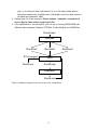
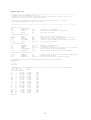
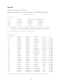
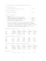
Manual of PEARLNEQ
(VERSION COMPATIBLE WITH FOCUS PEARL 3.3.3)
Aaldrik Tiktak1, Jos Boesten2
1) MNP, PO BOX 1, 3720 AH BILTHOVEN, the Netherlands
2) Alterra, PO BOX 47, 6700 AA WAGENINGEN, the Netherlands
Tip: Start with the default example, provided with the package!!!
Release notes:
Values in table 6 of the PEARL manual should be replaced by the values
in this example (see appendix).
The previous version contained a series of small bugs. These bugs have
been fixed in this version.
The weighing factors for the measurements have changed: all
measurements are now given a weighing factor that equals the inverse
of each measured value, thus giving equal weight to all measurements.
According to recommendations of the FOCUS Kinetics Workgroup, the
initial mass in the system should be optimised. This recommendation
has been implemented in the current version.
A second example (example2.mkn) has been added.
This document describes the PEARLNEQ-PEST combination, which can be used to
obtain the half-life at reference temperature (DT50Ref), the desorption rate
coefficient (CofRatDes), and the multiplication factor for the non-equilibrium sorption
coefficient (FacSorNeqEql) in the case of sorption/desorption kinetics. If the
incubation experiment has been carried out at multiple temperatures, the molar
activation energy (MolEntTra) can be optimised simultaneously.
Precautionary remark
This PEARLNEQ software tool should be seen as an introduction to fitting results
experiments on long-term sorption kinetics to the PEARL sorption submodel.
PEARLNEQ shows you how PEST can be coupled to a fortran programme that
contains this PEARL sorption submodel (i.e. PEARLNEQ.EXE). PEARLNEQ should
not be seen as a ready-to-use tool. PEARLNEQ provides you with example input
files to the PEST optimisation package and shows you how to organise this
optimisation. We had to make a number of assumptions for generating these PEST
input files (e.g. upper and lower bounds of parameters, weighing factors for each
measurement, etc. etc.). We do not claim that these assumptions are defensible for
your problem; they are our best guesses at this moment.
While using PEARLNEQ, we noticed that very regularly the results depend on the
initial guesses of the parameters. Therefore we advise you to perform always a
1
number of runs with different initial guesses. We advise you also to analyse the
results very carefully (especially the confidence intervals of the estimated
parameters). We do not accept any responsibility for use of PEARLNEQ.
Running the example
The following steps must be followed.
1 Installation. PEARLNEQ is distributed in a self-extracting zip file. Run
unpack_pearlneq.exe and specify a path (e.g. c:\pearlneq). The package
contains three directories, i.e. Neq_Bin, pest and Neq_Example.
The Neq_Bin directory contains the PEARLNEQ executables,
PEARLNEQ.EXE and PEARLMK.EXE.
The PEST optimisation software is available in the pest directory. As PEST is
now available freeware (http://www.sspa.com/pest), we included the latest
version as of 29-10-2003 (version 7.0.1.). Separate installation of PEST is not
necessary.
The Neq_Example directory contains results from an example study, as
described in the PEARL user manual, page 51-54.
2 You can now run the example, to check if everything works and get experience
with the system. Go to the Neq_Example directory, and run the example,
example.bat.
The batch file will first call PEARLMK. This pre-processing program generates
the input files for PEST, i.e. example.pst, example.tpl and example.ins.
Than the optimisation starts. PEST calls PEARLNEQ several times (in the
example 39 times).
If you get an error message after the first step (PEARLMK), type control-break
to stop the process and check the error messages available in the
example.err file.
3 After successful optimisation, read the results from the file example.rec. The
relevant results, including parameter values, 95% confidence intervals and
correlation matrices can be found at the end of this file. PEST also generates
parameter sensitivity files etc. Details can be found in the PEST manual, which is
available in the PEST subdirectory of the package.
4 If you encounter errors during the second step, you can try running PEARLNEQ
directly. PEARLMK has created a file example.neq, which is the input file for
PEARLNEQ. Type ..\Neq_Bin\PEARLNEQ EXAMPLE. PEARLNEQ will create an output
file (example.out) and a log file (example.log). The output files are self-explaining.
5 You can use the XyWin program to make a graph. XyWin is available in the
neq_bin\xypearl directory of PEARLNEQ (the example job does this call for your):
..\Neq_Bin\xypearl\xywin –j example.job –W l
2
Run PEARL_Neq with your own data
1 Be sure that an appropriate incubation experiment has been carried out (see the
FOCUS PEARL user manual). The first step of optimising your own data consists
of editing the file example.mkn, which can be found in the example
subdirectory of the PEARLNEQ directory. Please make a copy of this file before
editing. An example of this input file is listed at the end of this appendix. The
following parameters must be provided:
TimEnd (d): The duration of the incubation experiment.
MasSol (g): The mass of dry soil incubated in each jar.
VolLiqSol (mL): Volume of liquid in the moist soil during incubation.
VolLiqAdd (mL): Volume of liquid added to the soil after incubation (i.e. the
amount of liquid added to perform a conventional desorption equilibrium
experiment).
CntOm (kg.kg-1): Mass fraction of organic matter in the soil.
ConLiqRef (mg L-1): Reference concentration in the liquid phase.
ExpFre (-): Freundlich exponent.
KomEql (L kg-1): coefficient of equilibrium sorption on organic matter.
MasIni (µg): The initial total mass of pesticide in each jar. In contrast to the
previous version of PEARLNEQ, this parameter will be optimised. There is no
default value for this parameter.
FacSorNeqEql (-): factor describing the ratio KF,ne/KF,eq. This parameter will be
optimised, but you have to specify an initial guess here. The default value is
0.5.
CofRatDes (d-1): the desorption rate coefficient. This parameter will be
optimised, but you have to specify an initial guess here. The default value is
0.01 d-1.
DT50Ref (d): the transformation half-life under reference conditions. applying
to the equilibrium domain. This parameter will be optimised, but you have to
specify an initial guess here. As a default value, you can use the ‘classical’
half-life, which applies to the total soil system (i.e. the equilibrium domain +
the non-equilibrium domain).
TemRefTra (C): The reference temperature, at which the half-life should be
known. The default values is 20 oC.
MolEntTra (kJ mol-1): the molar enthalpy of transformation. This parameter will
be optimised if you have carried out the experiment at multiple temperatures;
otherwise it is a model-input. If optimised, you have to specify an initial guess
here. The default value is 54 kJ mol-1.
table Tem (C): List of temperatures at which the incubation experiment has
been carried out. At least two temperatures must be specified.
table Observations: List of observations. The first column contains the time
(d), the second column the temperature, column 3 contains the total mass of
pesticide in the system (µg), column 4 contains the concentration of pesticide
3
(µg L-1) in moist soil (then VolLiqAdd = 0) or in the water phase after a
desorption experiment (in which case VolLiqAdd is not zero) and column 5
contains the characters ‘OBS’.
2. Repeat step 2-5 in the example. Please replace “example” everywhere it
occurs by the name of the copied input file.
3. If the optimization is not succesfull, you can try re-running PEARLNEQ with
different initial guesses of MasIni, DT50Ref, FacSorNeqEql and CofRatDes.
RunId.mkn
PearlMk
RunId.ins
If Converged
RunId.rec
RunId.tpl
Pest
RunId.neq
PearlNeq
RunId.out
Figure 1 Dataflow diagram for the PEARLNEQ-PEST combination
4
RunId.pst
Example input file
*----------------------------------------------------------------------------------------* STANDARD FILE for PEARLMK version 3.3.3
* Program to fit the half-life, activation energy and desorption rate in the case of
* pesticide that show kinetic sorption behaviour
*
* This file is intended for use with the PEST program (Doherty et al., 1991).
* Copyright MNP/RIVM/Alterra 2003, 2005, 2006.
*
*----------------------------------------------------------------------------------------* Model control
Yes
ScreenOutput
0.0
TimStart
500.0
TimEnd
0.01
DelTim
(d)
(d)
(d)
Start time of experiment
Duration of the incubation experiment
Time step of output
* System characterization
45.36
MasSol
54.64
MasIni
6.64
VolLiqSol
0.0
VolLiqAdd
0.047
CntOm
(g)
(ug)
(mL)
(mL)
(kg.kg-1)
Mass of soil in the icubation jars
Initial guess of the initial mass of pesticide
Volume of liquid in the moist soil
Volume of liquid ADDED for equilibrium experiment
Organic matter content
* Sorption parameter
1.0
ConLiqRef
0.87
ExpFre
2.1
KomEql
0.5
FacSorNeqEql
0.01
CofRatDes
(mg.L-1)
(-)
(L.kg-1)
(-)
(d-1)
Reference liquid content
Freundlich exponent
Coefficient of equilibrium sorption on org. matter
Initial guess of ratio Kfneq/Kfeql
Initial guess of desorption rate coefficient
* Transformation parameters
10.00
DT50Ref
20.0
TemRefTra
54.0
MolEntTra
(d)
(C)
(kJ.mol-1)
Initial guess of half-life at reference temperature
Reference temperature
Initial guess of molar activation energy
* Temperature at which the incubation experiments are being carried out
table Tem (C)
1 5.0
2 15.0
end_table
* Measured mass and concentration of pesticide as a function of time and temperature
* Tim Tem Mas
Con
* (d) (C) (ug)
(ug/L)
table Observations
2
5
51.6300
5.7285
OBS
10
5
50.5900
5.0560
OBS
42
5
46.0200
3.6635
OBS
87
5
38.6100
2.9320
OBS
157
5
32.8150
1.9280
OBS
244
5
25.8700
1.4650
OBS
358
5
20.3150
0.8820
OBS
451
5
9.4250
0.6015
OBS
2
15
51.3300
5.8955
OBS
6
15
47.3950
4.4425
OBS
10
15
45.0650
3.9510
OBS
42
15
23.1400
1.6470
OBS
87
15
10.8950
0.6710
OBS
157
15
3.1350
0.1525
OBS
244
15
1.4400
0.0305
OBS
358
15
0.4500
0.0000
OBS
451
15
0.1500
0.0000
OBS
end_table
5
Appendix
Results (last section of rec file)
These are the results of the default example, provided with the package.
OPTIMISATION RESULTS
Parameters ----->
Parameter
fsne
crd
dt50
masini
met
Estimated
value
0.600286
1.226317E-02
13.0062
56.0664
108.755
95% percent confidence limits
lower limit
upper limit
0.408681
0.791892
9.886449E-03
1.463989E-02
11.5100
14.5024
52.1243
60.0084
102.806
114.705
Note: confidence limits provide only an indication of parameter uncertainty.
They rely on a linearity assumption which may not extend as far in
parameter space as the confidence limits themselves - see PEST manual.
See file EXAMPLE.SEN for parameter sensitivities.
Observations ----->
Observation
o1
o2
o3
o4
o5
o6
o7
o8
o9
o10
o11
o12
o13
o14
o15
o16
o17
o18
o19
o20
o21
o22
o23
o24
o25
o26
o27
o28
o29
o30
o31
o32
o33
o34
Measured
value
51.6300
5.72850
50.5900
5.05600
46.0200
3.66350
38.6100
2.93200
32.8150
1.92800
25.8700
1.46500
20.3150
0.882000
9.42500
0.601500
51.3300
5.89550
47.3950
4.44250
45.0650
3.95100
23.1400
1.64700
10.8950
0.671000
3.13500
0.152500
1.44000
3.050000E-02
0.450000
0.00000
0.150000
0.00000
Calculated
value
55.5316
5.39742
53.4684
5.08081
46.2635
4.06320
38.2669
3.09390
29.0458
2.16483
20.9646
1.47675
13.8380
0.932184
9.90684
0.648450
53.3843
5.17830
48.4369
4.62304
43.9959
4.12910
21.3140
1.70735
8.98367
0.544736
3.26320
0.131795
1.24259
3.866613E-02
0.399623
1.077987E-02
0.162574
4.019330E-03
Residual
-3.90156
0.331082
-2.87844
-2.480823E-02
-0.243511
-0.399703
0.343149
-0.161897
3.76922
-0.236828
4.90536
-1.175005E-02
6.47702
-5.018437E-02
-0.481840
-4.694962E-02
-2.05426
0.717199
-1.04190
-0.180537
1.06909
-0.178099
1.82600
-6.034768E-02
1.91133
0.126264
-0.128203
2.070505E-02
0.197406
-8.166130E-03
5.037676E-02
-1.077987E-02
-1.257429E-02
-4.019330E-03
Weight
1.9000E-02
0.1750
2.0000E-02
0.1980
2.2000E-02
0.2730
2.6000E-02
0.3410
3.0000E-02
0.5190
3.9000E-02
0.6830
4.9000E-02
1.134
0.1060
1.663
1.9000E-02
0.1700
2.1000E-02
0.2250
2.2000E-02
0.2530
4.3000E-02
0.6070
9.2000E-02
1.490
0.3190
6.557
0.6940
32.79
2.222
1.000
6.667
1.000
See file EXAMPLE.RES for more details of residuals in graph-ready format.
6
Group
no_name
no_name
no_name
no_name
no_name
no_name
no_name
no_name
no_name
no_name
no_name
no_name
no_name
no_name
no_name
no_name
no_name
no_name
no_name
no_name
no_name
no_name
no_name
no_name
no_name
no_name
no_name
no_name
no_name
no_name
no_name
no_name
no_name
no_name
See file EXAMPLE.SEO for composite observation sensitivities.
Objective function ----->
Sum of squared weighted residuals (ie phi)
=
0.4297
=
0.8997
Correlation Coefficient ----->
Correlation coefficient
Analysis of residuals ----->
All residuals:Number of residuals with non-zero weight
Mean value of non-zero weighted residuals
Maximum weighted residual [observation "o13"]
Minimum weighted residual [observation "o30"]
Standard variance of weighted residuals
Standard error of weighted residuals
=
34
= 1.3161E-02
= 0.3174
= -0.2677
= 1.4816E-02
= 0.1217
Note: the above variance was obtained by dividing the objective
function by the number of system degrees of freedom (ie. number of
observations with non-zero weight plus number of prior information
articles with non-zero weight minus the number of adjustable parameters.)
If the degrees of freedom is negative the divisor becomes
the number of observations with non-zero weight plus the number of
prior information items with non-zero weight.
Parameter covariance matrix ----->
fsne
crd
dt50
masini
met
fsne
8.7787E-03
8.4444E-05
-5.6502E-02
6.4073E-02
0.1016
crd
8.4444E-05
1.3507E-06
-4.5078E-04
6.0200E-04
6.0023E-04
dt50
-5.6502E-02
-4.5078E-04
0.5353
-0.5756
-1.463
masini
6.4073E-02
6.0200E-04
-0.5756
3.716
-0.8663
met
0.1016
6.0023E-04
-1.463
-0.8663
8.463
masini
0.3548
0.2687
-0.4081
1.000
-0.1545
met
0.3727
0.1775
-0.6872
-0.1545
1.000
Parameter correlation coefficient matrix ----->
fsne
crd
dt50
masini
met
fsne
1.000
0.7755
-0.8242
0.3548
0.3727
crd
0.7755
1.000
-0.5301
0.2687
0.1775
dt50
-0.8242
-0.5301
1.000
-0.4081
-0.6872
Normalized eigenvectors of parameter covariance matrix ----->
fsne
crd
dt50
masini
met
Vector_1
1.4335E-02
-0.9999
9.4905E-04
7.8350E-05
7.0894E-05
Vector_2
-0.9842
-1.4279E-02
-0.1745
-1.4702E-02
-1.9859E-02
Vector_3
0.1744
1.5744E-03
-0.9453
-0.2006
-0.1889
Vector_4
-2.2879E-02
-1.9999E-04
0.2229
-0.9685
-0.1084
Vector_5
1.1198E-02
6.4642E-05
-0.1618
-0.1467
0.9758
Eigenvalues ----->
4.7821E-07
1.7663E-03
0.1313
7
3.753
8.837