Download 3. Data input program

Universal Mechanism 5.0
3.
3-1
Chapter 3. Data input program
DATA INPUT PROGRAM.......................................................................................................... 3-4
3.1.1.
Setup of symbolic generation of equations of motion......................................................................... 3-5
3.1.1.1.
Delphi....................................................................................................................................... 3-5
3.1.1.2.
C++ .......................................................................................................................................... 3-6
3.1.2.
Paths to external subsystems ............................................................................................................. 3-6
3.1.3.
Paths to user’s units .......................................................................................................................... 3-7
3.1.4.
General options of the Input program ................................................................................................ 3-7
3.1.5.
Component libraries ......................................................................................................................... 3-8
3.2.
Main menu commands and tool panel ........................................................................ 3-9
3.2.1.
3.2.2.
3.2.3.
3.2.4.
3.2.5.
3.2.6.
3.3.
File................................................................................................................................................... 3-9
Object ............................................................................................................................................ 3-10
Tools .............................................................................................................................................. 3-10
Edit ................................................................................................................................................ 3-11
Help ............................................................................................................................................... 3-11
Tool panel ...................................................................................................................................... 3-11
Object constructor..................................................................................................... 3-12
3.3.1.
Basic elements of constructor.......................................................................................................... 3-12
3.3.1.1.
List of object elements ............................................................................................................ 3-13
3.3.1.2.
Animation window ................................................................................................................. 3-15
3.3.1.2.1. Visualization of object elements........................................................................................... 3-15
3.3.1.2.2. Modes of animation window ................................................................................................ 3-15
3.3.1.2.3. Basic system of coordinates, pop-up menu ........................................................................... 3-16
3.3.1.2.4. Tool bar ............................................................................................................................... 3-17
3.3.2.
Data inspector and some features of object element description ....................................................... 3-18
3.3.2.1.
List of object elements and access to element description......................................................... 3-18
3.3.2.2.
General object parameters and options..................................................................................... 3-19
3.3.2.3.
Lists of elements of a definite type .......................................................................................... 3-20
3.3.2.4.
Data types ............................................................................................................................... 3-21
3.3.2.4.1. Numeric constants ............................................................................................................... 3-21
3.3.2.4.2. Identifiers ............................................................................................................................ 3-21
3.3.2.4.3. Standard functions and constants.......................................................................................... 3-23
3.3.2.4.4. Constant symbolic expression .............................................................................................. 3-25
3.3.2.4.5. Expression – explicit function .............................................................................................. 3-25
3.3.2.4.6. External functions ................................................................................................................ 3-26
3.3.2.4.7. External identifiers............................................................................................................... 3-27
3.3.2.4.8. Time function from text file ................................................................................................. 3-28
3.3.2.4.9. Timetable as a method of description of time functions......................................................... 3-29
3.3.3.
Curve editor ................................................................................................................................... 3-30
3.3.3.1.
Modes of curve editor ............................................................................................................. 3-30
3.3.3.2.
Tool bar .................................................................................................................................. 3-30
3.3.3.3.
Adding, positioning, and deleting separate point on a curve ..................................................... 3-31
3.3.3.4.
Selecting, copying, deleting and moving fragments and curves ................................................ 3-31
3.3.3.5.
Closing curve .......................................................................................................................... 3-32
3.3.3.6.
Smoothing .............................................................................................................................. 3-32
3.3.3.7.
Usage of clipboard for creating curves and functions ............................................................... 3-33
3.3.4.
Hot keys ......................................................................................................................................... 3-33
3.3.4.1.
Constructor ............................................................................................................................. 3-33
3.3.4.2.
Inspector ................................................................................................................................. 3-33
3.3.4.3.
Animation window ................................................................................................................. 3-33
3.3.4.4.
Inspector tab with a list ........................................................................................................... 3-34
3.4.
Data Input.................................................................................................................. 3-35
3.4.1.
Data Input Sequence ....................................................................................................................... 3-35
3.4.2.
Input of subsystems ........................................................................................................................ 3-36
3.4.2.1.
Setting connection with external subsystems ........................................................................... 3-37
3.4.3.
Standard interface for setting local system of coordinates ................................................................ 3-38
3.4.4.
Assigning Graphical Image to Object Element ................................................................................ 3-40
3.4.5.
Assignment of graphic images to rods, linear and bipolar force elements ......................................... 3-40
3.4.6.
Input of Graphical Objects .............................................................................................................. 3-40
Universal Mechanism 5.0
3-2
Chapter 3. Data input program
3.4.6.1.
Lists of Graphical Objects and Graphical Elements.................................................................. 3-41
3.4.6.2.
Input of graphical elements (GE)............................................................................................. 3-42
3.4.6.2.1. Polyhedron .......................................................................................................................... 3-42
3.4.6.2.2. Ellipse ................................................................................................................................. 3-43
3.4.6.2.3. Box ..................................................................................................................................... 3-43
3.4.6.2.4. Spiral................................................................................................................................... 3-44
3.4.6.2.5. Ellipsoid .............................................................................................................................. 3-44
3.4.6.2.6. Cone.................................................................................................................................... 3-45
3.4.6.2.7. Parametrical GE................................................................................................................... 3-45
3.4.6.2.8. Profiled GE ......................................................................................................................... 3-47
3.4.6.2.9. Z-surface ............................................................................................................................. 3-49
3.4.6.2.10. GO as a graphic element .................................................................................................... 3-51
3.4.6.3.
GE colors................................................................................................................................ 3-52
3.4.6.4.
Position and Orientation of GE ................................................................................................ 3-53
3.4.6.5.
Inertia parameters of GE ......................................................................................................... 3-54
3.4.6.6.
Curve editor ............................................................................................................................ 3-55
3.4.7.
Input of bodies................................................................................................................................ 3-58
3.4.7.1.
Image and visualization of a body. Body-fixed SC................................................................... 3-59
3.4.7.2.
Inertia parameters ................................................................................................................... 3-60
3.4.7.3.
Adjust/adjusted joint ............................................................................................................... 3-60
3.4.7.4.
Connection points ................................................................................................................... 3-60
3.4.7.4.1. Adding general connection points ........................................................................................ 3-61
3.4.7.4.2. Adding oriented connection points ....................................................................................... 3-62
3.4.7.4.3. Adding vectors .................................................................................................................... 3-64
3.4.7.5.
3D Contact ............................................................................................................................. 3-65
3.4.8.
Joints and force elements: some features of description ................................................................... 3-68
3.4.8.1.
Assignment of bodies .............................................................................................................. 3-68
3.4.8.2.
Type of element ...................................................................................................................... 3-68
3.4.8.3.
Attachment points ................................................................................................................... 3-69
3.4.8.4.
Visual assignment of bodies and attachment points .................................................................. 3-69
3.4.8.5.
Transformation of coordinates ................................................................................................. 3-69
3.4.9.
Input of joints ................................................................................................................................. 3-70
3.4.9.1.
Visualization of joints ............................................................................................................. 3-70
3.4.9.2.
Weight of joint........................................................................................................................ 3-70
3.4.9.3.
Convertion of joint type .......................................................................................................... 3-70
3.4.9.4.
Input of rotational and translational joints ................................................................................ 3-72
3.4.9.5.
Input of 6 d.o.f. joint ............................................................................................................... 3-74
3.4.9.6.
Input of joint of generalized type ............................................................................................. 3-76
3.4.9.6.1. Elementary transformation tc ............................................................................................... 3-76
3.4.9.6.2. Elementary transformation rc ............................................................................................... 3-76
3.4.9.6.3. Elementary transformations tv, rv......................................................................................... 3-77
3.4.9.6.4. Elementary transformations tt, rt .......................................................................................... 3-77
3.4.9.7.
Input of quaternion joint .......................................................................................................... 3-79
3.4.9.8.
Input of rod constraint ............................................................................................................. 3-80
3.4.10. Input of force elements ................................................................................................................... 3-81
3.4.10.1. Input of bipolar force elements ................................................................................................ 3-81
3.4.10.1.1. Linear force element .......................................................................................................... 3-82
3.4.10.1.2. Friction and elastic-frictional elements ............................................................................... 3-82
3.4.10.1.3. Elastic-frictional element 2................................................................................................. 3-82
3.4.10.1.4. Viscous-elastic element...................................................................................................... 3-83
3.4.10.1.5. Points (numbers)................................................................................................................ 3-83
3.4.10.1.6. Points (expressions) ........................................................................................................... 3-86
3.4.10.1.7. Hysteresis .......................................................................................................................... 3-88
3.4.10.1.8. Fancher leaf spring ............................................................................................................ 3-90
3.4.10.1.9. Impact (bump stop) ............................................................................................................ 3-90
3.4.10.1.10. List of forces .................................................................................................................... 3-91
3.4.10.2. Input of scalar torque force element......................................................................................... 3-92
3.4.10.3. Input of generalized linear force elements................................................................................ 3-94
3.4.10.3.1. Some features of description of elastic element................................................................... 3-95
3.4.10.4. Input of contact force elements................................................................................................ 3-97
3.4.10.4.1. Points-Plane contact ........................................................................................................... 3-97
3.4.10.4.2. Sphere-Plane contact.......................................................................................................... 3-98
3.4.10.4.3. Circle-Plane contact ........................................................................................................... 3-99
Universal Mechanism 5.0
3-3
Chapter 3. Data input program
3.4.10.4.4. Sphere-Sphere contact........................................................................................................ 3-99
3.4.10.4.5. Points / Sphere / Circle - Z surface contact ....................................................................... 3-100
3.4.10.5. Input T-forces ....................................................................................................................... 3-101
3.4.10.6. Special forces ....................................................................................................................... 3-102
3.4.10.6.1. Gearing............................................................................................................................ 3-102
3.4.10.6.2. Cam................................................................................................................................. 3-103
3.4.10.6.3. Spring.............................................................................................................................. 3-105
3.4.10.6.4. Rack and pinion ............................................................................................................... 3-107
3.4.10.6.5. Bushings.......................................................................................................................... 3-109
3.5.
UM Components.......................................................................................................3-111
3.5.1.
Basic notions ................................................................................................................................ 3-111
3.5.2.
Adding a component in visual mode ............................................................................................. 3-112
3.5.2.1.
Visual adding generalized linear elastic or viscous-elastic forces............................................ 3-112
3.5.2.2.
Saving object data ................................................................................................................. 3-116
3.6.
Generation of equations of motion...........................................................................3-117
3.6.1.
3.6.2.
3.7.
Numeric-iterative method ............................................................................................................. 3-117
Symbolic method.......................................................................................................................... 3-117
Compilation of equations of motion.........................................................................3-119
Universal Mechanism 5.0
3-4
Chapter 3. Data input program
3. Data input program
Program for description of objects is intended for creation, correction multibody systems, as
well as for automatic generation of equations of motion and their compilation. List of files in the
program:
bin\UMInput.exe
bin\um.rsc (file of string resources)
bin\GraphRes.rsc (file of string resources)
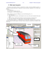
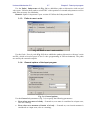
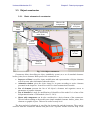
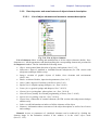
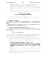
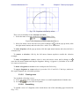
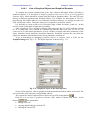
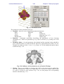
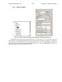
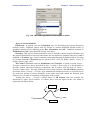
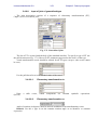
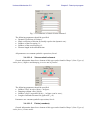
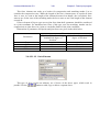
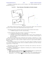
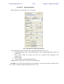
Basic elements of program (UMInput.exe) are the following (Fig. 3.1):
· The main menu;
· The tool panel with buttons, which duplicate some most often used command of the main
menu;
· The set of sheets with typical elements for visual construction of simple objects;
· The object constructor – the main tool for object description and correction.
The Data input program is a multitasking tool, which allows opening several constructors
with description of various objects. An object, whose constructor is placed over all others, is the
active one.
Sheets with
components
Constructor
of objects
Main
menu
Buttons duplicating main
menu
Element tree
Data
inspector
List of
identifiers
Animation
window
Fig. 3.1
Universal Mechanism 5.0
3-5
Chapter 3. Data input program
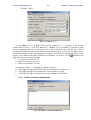
Options of Input program
To set or modify options of the Input program
· Run UMInput.exe;
· Call the option window with the Tools | Options main menu command;
· Use the OK button of the window to store changes in the computer registry.
3.1.1. Setup of symbolic generation of equations of motion
UM generates equations of motion of objects with the help of a built-in specialized computer
algebra system. To simulate the object dynamics, the equations should be compiled with the help
of an external compiler (Delphi 4.0-7.0, Visual C++ 5.0-6.0, Borland C++ Builder 3.0-5.0, BDS
2005-2006), which is not delivered with UM. First of all, make sure that a proper compiler is
installed on your computer or on a server. Then use the General tab to set the default external
compiler. In fact, UM can use numeric-iterative method of the generation of equations of motion
without an external compiler.
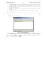
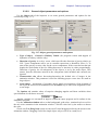
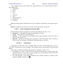
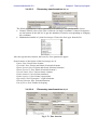
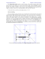
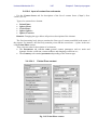
3.1.1.1.
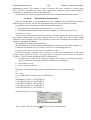
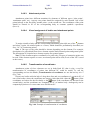
Delphi
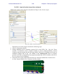
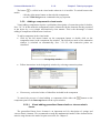
Fig. 3.2. Paths to Delphi
Use the Paths | Delphi tab (Fig. 3.2) to specify paths to a Delphi compiler and the Delphi
VCL files. If the current computer has Delphi 4.0-7.0 (or higher) installed, it is enough to click
the Search Delphi button to set the paths. If Delphi can be found in the local net try to find it
automatically using the same button and the option Net turned on. In this case the paths will be
found if the registry of the corresponding net computer is available for reading. If reading of the
registry is not allowed, the paths should be set manually. To do this, use the
buttons in the
right hand side of two boxes and find
· Delphi compiler dcc32.exe (usually [path to Delphi]\bin),
· Directory containing Delphi VCL *.dcu files (usually [path to Delphi]\lib).
Example:
· D:\Delphi5\bin\dcc32.exe,
· D:\Delphi5\lib.
Universal Mechanism 5.0
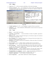
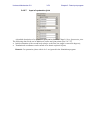
3.1.1.2.
3-6
Chapter 3. Data input program
C++
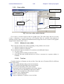
Fig. 3.3. Paths to C++
Use the Paths | C++ tab (Fig. 3.3) to specify paths to a C++ compiler. If the current
computer has Visual C++ 5.0-6.0 or Borland C++ Builder 3.0-5.0, installed, it is enough to click
the corresponding button to set the paths. If C++ can be found in the local net, try to find it
automatically using the same button and the option Net turned on. In this case the paths will be
found if the registry of the corresponding net computer is available for reading. If reading of the
registry is not allowed, the paths should be set manually. To do this, use the
buttons in the
right hand side of two boxes and find
· C compiler cl.exe/bcc32.exe;
· Paths to C libraries (lib-files);
· Paths to the standard *.h files.
Example for Visual C++ installed on computer Suvorov:
· \\SUVOROV\Program Files\Microsoft Visual Studio\VC98\bin\cl.exe
· \\SUVOROV\Program Files\Microsoft Visual Studio\VC98\lib
· \\SUVOROV\Program Files\Microsoft Visual Studio\VC98\Include
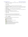
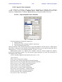
3.1.2. Paths to external subsystems
Fig. 3.4. Paths to external subsystem
Universal Mechanism 5.0
3-7
Chapter 3. Data input program
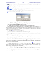
Use the Paths | Subsystems tab (Fig. 3.4) to add/delete paths to directories with external
subsystems. UM uses these paths to search DLL with equations of external subsystems as well as
other files necessary for simulation.
Remark. Option is important if your version of UM has the Subsystem Module.
3.1.3. Paths to user’s units
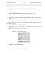
Fig. 3.5. Paths to user’s units and files
Use the Paths | Search paths (Fig. 3.5) tab to add/delete paths to directories with user’s units
and file, which are used as parts of user’s code (programming in UM environment). The paths
are used by the external compiler.
3.1.4. General options of the Input program
Fig. 3.6. General options
Use the General tab parameters (Fig. 3.6) to specify the following parameters:
· Error when zero mass of a body – if turned on, zero mass is considered as a input error,
else as a warning;
· Error when zero moment of inertia of a body – if turned on, zero inertia moment is
considered as a input error, else as a warning;
Universal Mechanism 5.0
·
·
·
·
3-8
Chapter 3. Data input program
The default language for automatically generated equations of motion and programming
in the UM environment; choice depends on the presented compiler (Sect. 3.1.1);
Open the last object – if checked, the latest active object will be opened automatically
when the Input program starts.
Open Pascal source files in – allows selecting an editor for programming on Pascal
language.
Open C source files in – allows selecting an editor for programming on C language.
Remark. Handling zero inertia parameters as an error is recommended for beginners only to
avoid the degeneration of the mass matrix at the simulation of objects. These options are ignored
for railway vehicle models.
3.1.5. Component libraries
Fig. 3.7. Component libraries
Use the Libraries tab to add or remove component library files. To add new component
library click the button
and select necessary file using standard dialog window Open. To
remove selected library use the button .
Universal Mechanism 5.0
3-9
Chapter 3. Data input program
3.2. Main menu commands and tool panel
3.2.1. File
·
·
New object (Ctrl+N) – opens constructor of a new object with the default name
UmObj[Index].
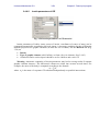
Open object (Ctrl+O) – calls a special dialog box for choice an existing object (Fig.
3.8). The dialog box contains a tree of objects found in the directory for reviewing
objects. To set the default path to the directory for reviewing objects use the menu
command Tools | Options and the page Paths | Objects in the window Options or use
the
button in the top edit box to choose the root directory and the Accept as default
button right after that.
Fig. 3.8. Open object dialog box
·
·
·
Use the F5 button or the pop-up menu to refresh the tree of objects in the Open object
dialog box. Use the upper edit box for changing the current directory.
Reopen – allows the user to open recently used objects.
Save (Ctrl+S) – saves the active object in the object directory. The command is executed
if the active object has been modified and the object directory has already been created. If
the directory does not exist, the Save as… command is executed.
Save as… – saves the active object in a directory pointed out by the user. Use the Save
as... dialog box to select or enter a path to the object including its name. If necessary, new
directories are created. The object takes the last directory in the path as its own name.
Fig. 3.9
·
Remark. Object name (i.e. the last directory in the path) must be an identifier, that is
then name contains the letters a…z, A…Z, digits 0…9, and the ‘_’. The first symbol
must be a letter.
Exit (Alt+X) – closes the program.
Universal Mechanism 5.0
3-10
Chapter 3. Data input program
3.2.2. Object
·
·
Verify data (F7) – verifies correctness and fullness of the object description.
Generate equations… (F8) – saves modified active objects, deletes old UMTask.dll file
of equations, and verifies the object description. If no errors are found, the window for
generating and compiling equations starts.
Fig. 3.10.
·
·
Compile equations (Ctrl+F9) – runs compiling of equations if they are generated.
Simulation… (F9) – verifies whether the UMTask.dll file exists for the active object and
runs the simulation.
3.2.3. Tools
·
·
·
·
·
·
·
·
·
·
·
·
Editor… – runs the built-in text editor.
Calculator of expressions… – runs the calculator of chains of symbolic expressions
(Sect. 3.3.2.4.2).
Inspector (F12) – brings to front the Data Inspector for the active object if it is located
on a separate window (Sect. 3.3.2).
List of elements (F11) – brings to front the List of elements for the active object if it is
located on a separate window (Sect.3.3.2.1).
Identifiers (Alt+I) brings to front the List of Identifiers of the active object if it is located
on a separate window.
List of windows (Alt+0) – calls the window containing the list of open windows.
Control File… (Alt+C) – opens the Control file for the active object in the text editor.
File of elements… – creates a file n[NameOfObject].txt in the object directory and opens
it in the text editor. The file contains lists of all the object elements (bodies, joints,
identifiers, force elements etc.) and their names.
Graphical converter… – opens a graphical converter of 3ds and ASC formats in the
UMI (UM) graphical format. Utility is used for import of external graphical objects.
Transformation of coordinates… (Alt+T) – opens the forms for transformation of
coordinates of points into different system of coordinates (Sect. 3.4.8.5).
Wizard of components… – tool for edition of component libraries.
List of components… – open window with the list of loaded components.
Universal Mechanism 5.0
·
3-11
Chapter 3. Data input program
Options – opens a dialog box with UM options: paths to external compiler, standard and
user’s libraries etc. (Sect. 0).
3.2.4. Edit
·
·
·
·
·
·
Copy in clipboard – copy parameters of selected elements to clipboard.
In clipboard as component – write parameters of the selected element and the graphic
object connected with it to clipboard. If the element has no graphical object the option is
disabled.
Copy into file… – write parameters of the selected element into file.
Save as component… – save parameters of the selected element and the graphic object
connected with it in file.
Insert – insert element/component from clipboard.
Read from file… – add all elements from file to the object.
3.2.5. Help
· Lessons – access to several lessons, teaching UM environment
It is recommended to study the lessons before working with UM.
· About – short information about UM version and the list of developers.
3.2.6. Tool panel
Buttons located on the tool panel have the following functions:
– creates a new object;
– opens an existing object;
– saves the active object;
– saves the active object with a new name;
– opens the text editor;
– opens symbolic calculator;
– verifies correctness of the active object description;
– generates and compile equations for the active object;
– compiles equations for the active object;
– runs simulation of the active object.
Universal Mechanism 5.0
3-12
Chapter 3. Data input program
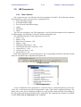
3.3. Object constructor
3.3.1. Basic elements of constructor
Sheets with
components
Main
menu
Constructor
of objects
Buttons duplicating
main menu
List of
elements
Inspector
of data
List of
identifiers
Animation
window
Fig. 3.11. Object constructor
Constructor allows describing an object (multibody system) as a set of standard elements:
bodies, joints, force elements. Basic parts of the constructor are
· Inspector of Data is used for input, modification and representation of object elements
as well as some other information about the object.
· Animation window gives the object image or its parts according to active elements
presented in the inspector. It can be use also for visual construction of models.
· List of elements presents the list of all object’s elements and organizes access to
parameters of separate elements
· List of identifiers is used for modification of identifiers of the model. It is a base of the
full parameterization of UM models (Sect.3.3.2.4.2).
· Sheets with components can be also considered as a basic element of the constructor.
This tool allows adding to the model some simple standard elements: bodies, joints, force
elements or graphic objects. This tool is used at a study level.
The drag-and-dock technology is used for the element list and the inspector. They can be
removed from the constructor window and placed on a separate window with the help of the
Universal Mechanism 5.0
3-13
Chapter 3. Data input program
mouse. If the list and the inspector are located as separate windows, the hot keys F11, F12, Alt+I
are used to bring them in front.
Separate location of the list and the inspector are used to increase the animation window size
when creating complex objects if necessary.
3.3.1.1.
List of object elements
An object is a multibody system, which consists of separate typical elements. Access to the
elements is realized by means of the list of elements (Fig. 3.11), visually (3.3.1.2) or with the
help of hot keys (3.3.3).
Fig. 3.12. List of object elements
Click on a list item (Fig. 3.12) causes appearance of the corresponding information in the
object data inspector (3.3.2). The list contains the following items:
· Object – general object options, object type, gravity, background color etc. (3.3.2.2).
· Subsystems – list of subsystems (wheelsets, vehicle suspensions, caterpillar, including
user’s subsystems in the object). For UM version with subsystem technique only.
· Images – list of images, which are used for visualization of the scene, bodies and force
elements (3.4.6).
· Bodies – list of bodies and their parameters (mass, moments on inertia, coordinates of
centers of mass etc., Sect.3.4.7).
· Joints – input of joints (rotational, translational etc.) as well as coordinates of bodies
(Sect.3.4.9).
· Wizard of forces – is not used in this UM version, a perspective future development for
construction of complex force models.
· Bipolar forces – list of bipolar forces, i.e. forces acting along the axis of element, which
connects two points of bodies (Sect.3.4.10.1). The force element is used for modeling
dampers, dogs etc.
· Linear forces – list of generalized linear force elements described by 6 ´ 6 stiffness or
damping matrices (Sect.3.4.10.2). The element is used for modeling springs, resistance of
the environment etc.
· Contact forces – list of force elements, which models contact interaction between bodies
(Sect.3.4.10.4).
Universal Mechanism 5.0
·
·
·
·
·
·
3-14
Chapter 3. Data input program
General forces – list of forces used mainly for their programming in the UM
environment (Sect. 3.4.10.5).
Special forces – models of special force interactions (gearing, cams, combined friction
etc. Sect.3.4.10.6).
3D Contact – setting for 3D contact model. Reserved for future use. For more detailed
description of using 3D Contact see Sect. 3.4.7.5.
Connections – a tool for assignment of attachment points for external joints and force
elements. For UM version with subsystem technique only.
Indices – internal UM indices of object elements and coordinates useful for
programming in the UM environment.
Summary – contains information about correctness of the object description as well as
lists of errors and warnings.
Universal Mechanism 5.0
3.3.1.2.
3-15
Chapter 3. Data input program
Animation window
3.3.1.2.1.
Visualization of object elements
The whole object or their active elements are visualized in the animation window depending
on the window mode (Sect.3.3.1.2.2). The following types of visual elements are used for
visualization of different elements:
· Graphic objects (GO) created by the user – for bodies, bipolar and generalized linear
force elements, special force elements spring, rod constraint images (Sect.3.4.6);
Fig. 3.13. Visualization commands
·
·
Icons – for force element of general type, linear and special force elements, connection
points, external elements (Fig. 3.13), the full object mode should be on (the
button);
Points.
Every type of listed visual elements has active regions, which are used for visual selection of
the corresponding object elements with the mouse.
· GO – the active region is the whole image;
· Icon – the active region is a small neighborhood of the left bottom part pointed out by the
arrow, e.g. for the joint icon:
·
·
Point – active region is a small neighborhood of the point.
Image – the set of bitmaps for representation of enabled degrees of freedom. Used for
joints only.
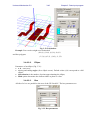
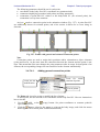
Fig. 3.14. Images for enabled degrees of freedom:
a) rotational; b) translational; c) three rotational (spherical joint).
3.3.1.2.2.
Modes of animation window
Animation window has two modes of visualization of an object. The button
menu are used to switch them.
· Whole object mode
or a pop-up
Universal Mechanism 5.0
3-16
Chapter 3. Data input program
The whole object is visualized. In this mode, a mouse click on the active region of an image
makes the corresponding element active (body, joint and force element, Sect. 3.3.1.2.1).
·
Single element mode
A separate element is visible in this mode: GO, body, joint or force element (together with
connected bodies).
Graphic mode (wire of surface graphics) can be changed with the help of two buttons
Orthogonal projection is turned on/off by means of the command Perspective of the
pop-up menu or the button:
Parameters of the orthogonal projection are modified with the help of the Window
parameters command of the pop-up menu.
3.3.1.2.3.
Basic system of coordinates, pop-up menu
The basic system of coordinates (SC0) is optionally presented in the animation window. Use
the Coordinate system command of the pop-up menu to visualize of hide the axes. Coordinates
of all elements attached the base must be given in this SC. A color principle is used to identify
the SC0 axes (RGB):
· axis X – Red;
· axis Y – Green;
· axis Z – Blue.
A coordinate grid coincides with one of the coordinate planes. Use the Window parameters
command of the pop-up menu to change the grid size and step.
Use the right mouse button to call a pop-up menu (Fig. 3.15).
Fig. 3.15
Universal Mechanism 5.0
3-17
Chapter 3. Data input program
Menu commands:
· Orientation – choice of one of the standard object orientations;
· Grid – choice of one of the standard grid locations;
Click an image of the SC0 axis to set the grid perpendicular to the corresponding axis
· Rotational style – choice of style of rotation for objects in the animation window: Zstyle used by default (from UM 3.0), On sphere – the style usually used in CAD
systems.
· Selection style – the style of graphical visualization of an active element of the object
(image contours or box rounding the element image);
· Coordinate system – turn on/off visualization of SC0;
· Window parameters – call of a window with perspective and grid parameters;
· Smoothing – turn on/off of smoothing mode;
· Perspective – turn on/off of orthogonal projection;
· Background color – setting the background color of the animation window;
· Contour graphic mode – is used to obtain contrast black-and-white image which is
suitable for printing.
· Show icons – is used for visualization of icons for joints, force element of general type,
generalized linear force element etc. (for the whole object mode in the animation window
only, Sect.3.3.1.2.2);
· Mode – switching the animation window modes (whole object / active element,
Sect.3.3.1.2.2).
3.3.1.2.4.
Tool bar
– Copy the window to clipboard or to a file (bmp);
– Zoom in the selected area of animation window;
– Show all (F9).
– Zoom in/out of a selected point on the object: click the button and immediately
click the left/right mouse button on an image point to zoom in/out the object and to
shift the point in the window center. Use also Alt+Shift + mouse click on an object
point;
– Shift mode (Ctrl + left mouse button);
– Zoom mode (Shift + left mouse button);
– Rotation mode (left mouse button);
– Choice of wire or surface graphics mode;
– Turn on/off perspective;
– Choice of one of standard views;
– Switch full object / single element mode (Sect.3.3.1.2.2);
– Show joint images.
See also Sect.3.3.4.3 for a list of hot keys.
Universal Mechanism 5.0
3-18
Chapter 3. Data input program
3.3.2. Data inspector and some features of object element description
3.3.2.1.
List of object elements and access to element description
Fig. 3.16. List of object elements
List of elements allows creating and modification of all the object elements (bodies, force
elements etc.). All the parameters and data describing the corresponding element are presented in
the Inspector window. The list included the following items:
· Object: some general data (direction of gravity) and options, Sect.3.3.2.2
· Subsystems: input of standard or included/external subsystems (for UM version with
subsystem technique abilities only)
· Images: creation of graphic objects of bodies, force elements and environment
(Sect.3.4.6)
· Bodies: creation of bodies, input inertia parameters (Sect.3.4.7)
· Joints: joints, degrees of freedom, joint forces (Sect.3.4.9)
· Bipolar forces (bipolar springs, dampers, etc., Sect.3.4.10.1)
· Linear forces (general springs and dampers, Sect. 3.4.10.2)
· Contact forces (point-plane, sphere-plane, etc., Sect. 3.4.10.4)
· General forces (usually for external programming of forces, Sect. 3.4.10.5)
· Special forces (gearing, cams etc., Sect. 3.4.10.6)
· Connections: connection of external elements (for UM version with subsystem technique
abilities only)
· Indices: useful information on indices of all the elements of the object
· Summary: information about correctness of the object description as well as list of errors
and warnings
Remark. Access to parameters of visualized elements can be achieved by clicking the
element image in the animation window if the window is in the whole object mode
(Sect.3.3.1.2.2).
Universal Mechanism 5.0
3.3.2.2.
3-19
Chapter 3. Data input program
General object parameters and options
Use the Object tab of the inspector to set some general parameters and options for the
current object (Fig. 3.17).
Fig. 3.17. Object general parameters and options
·
·
·
·
Type of object – General or Railway Vehicle (for program version with support of
dynamics of railway vehicles only).
Direction of gravity is set by a vector, which specifies the direction of gravity relative to
SC0. Vector components can be set as constant expressions or identifiers (Sect. 0). To
turn off the gravity set zero value for the vector components. If the vector has not the unit
length, the acceleration of the free falling decreases or increases its value proportionally.
Direction of gravity for all subsystems of the objects is set by the main object. This
means, that the directions entered in the subsystems (both included and external) are
ignored.
Characteristic size allows decreasing/increasing the default size of images in the
animation window. This parameter is used for obtaining proper vector sizes for small or
large objects.
Scene image – assignment of a graphic object, which corresponds to fixed elements of
the object as well as to environment. Press the Delete key to cancel the assignment of the
scene image.
The Options tab contains values of stepwise changing angular and linear variables when
special buttons in edit boxes are used
Angular variables are measured in degrees within the Input program and in radians in the
Simulation program.
Use the Animation window tab to set the background, grid colors, rotational style as well as
the axis color saturation in the animation window. Click the color box by the mouse to choose
the color.
Check on/off the Drag body option to turn on/off visual dragging bodies by the mouse in the
animation window. Dragging is used for simple object only as well as at a study level.
Universal Mechanism 5.0
3.3.2.3.
3-20
Chapter 3. Data input program
Lists of elements of a definite type
Each object (multibody system) is presented by sets of elements, most of which are grouped
as lists. Every list contains elements of a single type, e.g., lists of bodies, joints, bipolar force
elements and so on. Each element of a list has its own name, which is an arbitrary set of
symbols. The name of element is the base of its identification, and it must be unique within the
corresponding list, that is, it is not allowed setting one name for two elements of the same type
(e.g., for two bodies). Elements of different lists as well as elements, which belong to different
subsystems, may have the same names. So, the body and its image (or some joint) can have
equal names.
Standard interface possibilities are used to manage the lists within the data inspector.
a
b
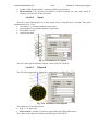
Fig. 3.18. Lists
Fig. 3.18a shows an empty list in the inspector, Fig. 3.18b shows the list, which contains
several elements (bodies). Every element of the list has its own tab (or page). The name of a
page coincides with the name of the corresponding element.
Edit box for the name and three buttons are located in the top of the tab:
– adds a new element to the list;
– creates an exact copy of the current element and adds it to the list;
– deletes the current element.
See also Sect. 3.3.4.4.
Remark
Press the Enter key after modification of the name else the changes can be lost.
Universal Mechanism 5.0
3.3.2.4.
3-21
Chapter 3. Data input program
Data types
Information about each element of an object (element parameters) is entered in boxes of the
data inspector. UM uses several standard data types. The user must know features of each data
type to work with UM correctly.
A very important feature of object description using UM is the data parameterization. This
means that many element parameters could be set not only by its numeric values but by
expressions including numbers, identifiers, operations and functions. Consider the basic types of
data presented in UM.
3.3.2.4.1.
Numeric constants
UM uses standard syntax for numbers.
Examples: 1.23, 0.256e-3
3.3.2.4.2.
Identifiers
Identifier is a set of symbols, which includes Latin letters, digits and character “_”.
The first symbol in the identifier cannot be a digit or character “_”.
Identifiers with the character “_” as the first symbol are reserved for internal presentation of
identifiers in equations of motion generated by the program.
Reserved words of Pascal and C languages cannot be used as identifiers.
The program verifies syntax of entered expressions. If a new identifier is found, it is added to
the list of identifiers of the object (Sect.3.3.1).
Example of correct identifiers:
mass_1 length_of_rod cdiss cstiff
Examples of wrong identifiers:
2mass – the first symbol is the digit 2;
_length – the first symbol is the character “_”;
mass% - prohibited character “%”;
do, as, while – reserved words of the Pascal language.
There exist two types of identifiers:
· Identifier – number;
· Identifier – expression.
Values of identifiers of the first type can be changed both in the Input and in the Simulation
programs. Identifiers of the second type are presented by arbitrary expressions, which include
· numbers;
· identifiers of the first and the second types;
· standard functions (Sect. 3.3.2.4.3).
Expressions for identifiers of the second type are entered in the List of Identifiers. Chains of
calculations may be programmed with the help of identifiers of the second type.
An example of a chain including identifiers of the both types is shown below.
Name
Expression
Value
Comments
Mass
1.12
Mass of rod
length
0.55
Length of rod
ix
mass*length^2/12
0.0282333333
Moment of inertia of the rod relative to X axis
iy
ix
0.0282333333
Moment of inertia of the rod relative to Y axis
Remark. Expression can only include identifiers located above the current identifier.
Universal Mechanism 5.0
3-22
Chapter 3. Data input program
The same principle is used in the built-in calculator (the menu Tools | Symbolic calculator
command).
Universal Mechanism 5.0
3.3.2.4.3.
3-23
Chapter 3. Data input program
Standard functions and constants
The following standard functions are used for description of data of several types (explicit
function, identifiers-expressions):
· sin, cos – trigonometric functions, arguments are set in radians;
· arcsin, arccos, arctan – inverse trigonometric functions (rad);
· arctan2(x, y) computes an angle a, tan a = x / y in radians in the interval from -p to p;
quadrant for the angle is defined by signs of arguments x,y as if x = sin a, y = cos a ;
·
·
·
exp – natural exponent;
ln – natural logarithm;
abs – absolute value;
·
ì 1, x > 0
ï
sign – sign (x ) = í 0, x = 0
ï- 1, x < 0
î
·
·
·
·
·
^ – power function, the expression a^b corresponds to a b , the exponent must be an
integer if the base is negative;
sqr – square;
sqrt – root square;
ì1, x > 0
Heavi – Heavi(x) = í
î0, x £ 0
ì v1, c < 0
ï
if( c , v1 , v2 , v3) = ív 2, c = 0
ï v 3, c > 0
î
x1
h1
x0
x
h0
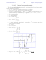
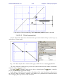
Fig. 3.19 Step function
·
ì
h0 , x < x0
ïï
x - x0
step( x , x0 , h0 , x1 , h1 )= íh0 + (h1 - h0 )d 2 (3 - 2d ), d =
x1 - x0
ï
ïî
h1, x > x1
Universal Mechanism 5.0
3-24
Chapter 3. Data input program
As a rule, the Step function is used for a smooth but fast transition of expression from one
value to another. Example of the function step( t , 0.1 , -0.2 , 0.15 , 0.3 ) is shown in Fig. 3.19.
Standard constants
pi : number p = 3.1415926536...
e : number e=2.7182818285
rtod: factor converting radians to degrees, e.g. arctan(1)*rtod=45;
dtor: factor converting degrees to radians, e.g. 90*dtor=pi/2.
Universal Mechanism 5.0
3.3.2.4.4.
3-25
Chapter 3. Data input program
Constant symbolic expression
An constant symbolic expression is an expression, which contains
· identifiers;
· numbers;
· additions, subtractions, divisions and multiplication;
· standard functions (Sect.3.3.2.4.3).
It is not allowed usage of identifier t (time)
Example of correct constant symbolic expressions:
sqrt(2)*b1+sqrt(a1+a2)/2
The constant symbolic expression can be used for most of the element parameters (inertia
and geometric parameters, coordinates of attachment points of the most type of force elements,
sizes of graphic elements, coefficients of stiffness and damping and so on). The corresponding
edit boxes in the data inspector have the standard interface
Fig. 3.20. Exit box for constant expressions
The letter ‘c’ in the right top part of the box points out that the parameter can be a constant
expression. Double click the box or use the pop-up menu to call a tool for visual construction of
the expressions.
3.3.2.4.5.
Expression – explicit function
The expression of this type includes
· numbers;
· identifiers;
· standard functions;
· standard variables (t, x, v, p1, p2, p – depending on type of function).
Double click the edit box or use the pop-up menu to call a tool for writing the expressions.
The corresponding window contains the list of identifiers and buttons with allowed functions.
Types of explicit functions:
· Function of time - t
The standard variable is t – time. The function is used for description of joints.
- Joint of generalized type, elementary transformation of types tt, rt (Sect. 3.4.9.6.4);
- Rotational and translational joints in the cases when the joint coordinate is an explicit
function of time (Sect. 3.4.9.4).
The corresponding edit boxes in the data inspector have the following standard interface
The letter ‘t’ in the right top part of the box points out that the expression is a time function.
· Force description force functions – x, v, t
Standard variables are t – time as well as two additional variables x (coordinate), v
(velocity).
The function is used for description of mathematical models of forces in the following cases:
Universal Mechanism 5.0
-
-
3-26
Chapter 3. Data input program
Description of a bipolar force element (the force type should be expression); x –
length of the element, v – time derivative of the length (Sect. 3.4.10.1);
Description of joint forces in the case of joint of general type (elementary
transformations rv, tv, type of force – expression, Sect. 3.4.9.6.3) as well as for
translational and rotational joints (Sect. 3.4.9.4); x – value of coordinate, v – its time
derivative;
Description of an axle force in the case of a special force of the Combined friction
type. The corresponding edit boxes in the data inspector have the following standard
interface (Fig. 3.21).
Fig. 3.21. Exit box for Pascal/C expressions
The letter ‘p’ – Pascal – in the right top part of the box points out that the data is a time function.
· Functions of description of parametrical graphic elements (Sect. 3.4.6.2.7).
Standard variables are p1, p2 parameterize a surface or a curve. The corresponding edit boxes
in the data inspector have the standard interface shown in Fig. 3.21.
· Description of Z –surfaces
Surfaces z = f ( x, y ) in 3D space are used in description of a Z – surface graphic element
(Sect. 3.4.6.2.9) as well as in Point -- Z –surface and Sphere - Z – surface contact force
elements.
Standard variables are p1, p2 parameterize a Z-surface. The corresponding edit boxes in the
data inspector have the standard interface shown in Fig. 3.21.
· Functions of description of profiled graphic elements (Sect. 3.4.6.2.8).
A standard variable is p parameterizes the corresponding profile of section or an axis curve.
The corresponding edit boxes in the data inspector have the standard interface
shown in Fig. 3.21.
3.3.2.4.6.
External functions
Usage of external function is directly connected with programming in the UM environment
based on a Control file. As a rule, these functions are used when the corresponding mathematical
model is too complicated for description as an implicit function (Sect. 3.3.2.4.5).
There exist three types of external functions, which are different with respect to arguments.
· Time functions (t) are used for joint of generalized type, elementary transformation of
types tt,rt (Sect. 3.4.9.6.4) as well as for rotational and translational joints in the cases
when the joint coordinate is an explicit function of time (Sect. 3.4.9.4).
· Function of three arguments (x, v, t) are used for description of
- a bipolar force element (type of element – external, Sect. 3.4.10.1);
- a joint force and torque in the cases of joint of general type (elementary
transformations rv, tv, type of force – expression, Sect. 3.4.9.6.3) as well as for
translational and rotational joints (Sect. 3.4.9.4); x – value of coordinate, v – its time
derivative;
- an axle force in the case of a special force of the Combined friction type. The
corresponding edit boxes in the data inspector have the following standard interface
(Fig. 3.21).
· Function of two arguments (p1, p2) are used for description of Z-surfaces (surfaces given
by the function z = f(x, y)) in the cases of graphic element (type - Z-surfaces)
(Sect. 3.4.6.2.9) and contact forces (Z-sphere).
Universal Mechanism 5.0
3-27
Chapter 3. Data input program
To describe an external function, the user should enter its name (identifier) in the
corresponding edit box of the inspector without arguments, for instance,
Syntax rules for name of function as the same as for identifier (Sect. 3.3.2.4.2).
UM generates a template for each external function in the control file. This means, that
special functions will be added to the control file, where the external function will be initialized
by zero values. The user should rewrite the corresponding procedures.
Consider a template of a time function. Let the identifier alpha were used as the name of
external function. UM inserts the following procedure in the control file Cl[NameOfObject]:
procedure alpha( _isubs : integer; _t : real; var _Value, _dValue, _ddValue
: real_ );
var
_ : _platfVarPtr;
begin
_ := _PzAll[SubIndx[_isubs]];
_Value := 0;
_dValue := 0;
_ddValue := 0;
end;
The input parameters are _isubs (the global index of subsystem), _t – the current time value.
The output values: value of function (identifier _Value) as well as its first and second derivatives
(_dValue, _ddValue).
Wrong programming of derivatives leads to wrong simulation results.
Consider a template for a function of (t, x, v). Let the identifier bforce1 was used for external
function corresponding to a bipolar or joint force. UM inserts the following function in the
control file Cl[NameOfObject]:
function bforce1( _isubs : integer; _t, _x, v : real ) : real_;
var
_ : _vehicleVarPtr;
begin
_ := _PzAll[SubIndx[_isubs]];
Result := 0;
end;
The input parameters are _isubs (the global index of subsystem), _t – the current time value,
the current x and v values: _x, _v. The user should change the function code to calculate the
output value Result.
Remarks
1. Functions of the one and same type, which have coinciding identifiers, are identified. That
is, only one template of function or procedure will be generated for them in the control
file. Different identifiers must be used for external functions of different types.
2. Detailed information about the control file and programming in the UM environment can
be found in the corresponding chapter of the user’s manual.
3. The Simulation program calls external functions automatically.
4. After adding or deleting external functions, the user should verify the correctness of the
old control file.
3.3.2.4.7.
External identifiers
External identifiers give one of the possible forms for programming forces with complex
Universal Mechanism 5.0
3-28
Chapter 3. Data input program
mathematical model. This method is used exclusively for force elements of general type
(Sect. 3.4.10.5). Projections of a force and a moment are identifiers, which values should be
calculated in a standard procedure of the control file.
See the chapter devoted to programming in the UM environment for more information.
3.3.2.4.8.
Time function from text file
Here we consider how to set dependences on time of angular and translational coordinates
with the help of text files. The file can contain both full-scale test and simulation results.
Coordinates as time functions are realized in the following joints
· generalized joint, elementary transformations tt, rt (3.4.9.6.4);
· translational and rotational joints when the coordinate is a time function (3.4.9.4).
Format of a text file
A text file with a time function should contain two columns separated by space symbols. The
first column contains time in seconds starting with zero or small value. The second column
contains the corresponding values of the function in meters for a translational coordinate and in
radians for an angular coordinate.
First symbol in comment lines should be %.
The file should be created beforehand and located in the directory of the model, which uses it.
If UM does not find the file, zero value is set for the corresponding function.
Creation of files with a time function as a simulation result
Each plot in graphic windows can be saved in a text file after simulation of a UM model
(Chapt. 4, Sect. Graphical window | Copying graphs to clipboard, text file and file of calculated
variables). The file format matches the above requirements if
· % symbol is set as a prefix for comments (Chapt.4. Sect. Options of simulation program |
General), otherwise comments should be deleted from file manually;
· one variable is saved;
· time is laid off as abscissa.
Fragment of an automatically generated compatible text file with a time function:
%
% 1 - time
% 2 - dyWheelset4 [Lateral position of Wheelset4]
%
2.00000002337219E-7 2.82372854E-15
1.03125004097819E-2 2.03257468E-6
2.09375005215406E-2 7.46718570E-6
3.21874991059303E-2 1.76279409E-5
4.21875007450581E-2 3.07774899E-5
Standard interface for setting the file
Fig. 3.22. Time function from file
To set a name of the file, use the
button or write the name directly.
Universal Mechanism 5.0
3-29
Chapter 3. Data input program
Note 1. UM uses a spline interpolation of discrete file data to get function value in
intermediate time moments as well to compute the first and the second derivative, which are
necessary for simulation.
Note 2. The user should take care of a sufficient smoothness of data in file.
Note 3. When the current simulation time exceeds the latest time point in the file, the
function value is constant equal the latest one in the file.
3.3.2.4.9.
Timetable as a method of description of time functions
Timetable is a generalization of time function description by an expression. This method is
used if the function can be described by different symbolic expressions on several time intervals.
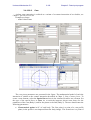
For instance, the function in figure satisfy the following relations:
vt , t Î [0, t1 ]
ì
f (t ) = í
îvt1 cos(w(t - t1 )), t Î [t1 , t 2 ]
A standard interface is used for setting such dependencies:
Use a pop up menu to add, delete insert a line into the timetable. The Plot item is used for
plotting the functions.
The table can contain any number of lines.
Time in the left column can be set by expressions (identifiers t1, t2 in our example).
Note 1. The user should take care of a continuity of the function.
Note 2. When the current simulation time exceeds the latest time point in the timetable, the
function value is constant equal the latest one in the table.
Universal Mechanism 5.0
3-30
Chapter 3. Data input program
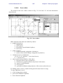
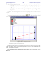
3.3.3. Curve editor
Type of smoothing
Tool bar
List of points
Curve
List of curves
Fig. 3.23. Curve editor and its elements
Curve editor is a tool for input of data in a graphic form. The editor allows the user to create
a curve, a function or a set of curves by a set of points. Here we consider some features of
working with the editor. Additional information about usage this tool for creation of 2D graphic
images can be found in Sect.3.4.6.6.
3.3.3.1.
Modes of curve editor
There exist two modes of the editor depending on the problem to be solved.
· Mode of creation of a set of curves
· Mode of creation of a function
The second mode imposes a number of restrictions and additional features:
· one curve only;
· ordering points according to abscissa value;
· plots the first and second derivative as well as a curvature in a separate window is
available.
3.3.3.2.
Tool bar
Consider functions of buttons on the tool bar. Note that sets of buttons differ for different
modes of the editor.
- left or right shift depending on the mouse button;
- up or down shift depending on the mouse button;
- zoom in/out depending on the mouse button;
- horizontal zoom in/out depending on the mouse button;
- vertical zoom in/out depending on the mouse button;
- zoom in of a rectangle area selected by the mouse;
- optimal view of inputted data;
- delete a selected fragment;
- copy to clipboard as a picture or as a text data;
Universal Mechanism 5.0
3-31
Chapter 3. Data input program
- preview of data in a 3D animation window (for 3D graphic elements only, Sect.
3.4.6.2.8).
- shift of the left border of the plot area;
- read data from file;
- save data to file;
- buttons for plotting the first and second derivative as well as a curvature in a
separate window is available for an inputted function;
- switch on/off a mode of equal scales along abscissa and ordinate axes;
- parameters of the plot area (Fig. 3.24).
Fig. 3.24. Parameters of the plot area
3.3.3.3.
Adding, positioning, and deleting separate point on a curve
There exist too methods for adding a point to a curve.
1. Double click by the left mouse button in the position off the adding point.
With this method a point can be added both to begin and the end of a non-closed curve, as
well as inside the closed or non-closed curve. When a point is added to the begin or to the end of
e curve, it is recommended to put it near the corresponding first or last point of the curve and
then to drag it to the desirable position.
2. Button
over the list of points (Fig. 3.23).
With this method you can add point to the end of the curve only.
Positioning the point means setting its desirable position. Two methods are realized for this
purpose.
1. Positioning by the list of points.
Find the point in the list, e.g. by clicking on its image in the plot area, and set its new
coordinates.
2. Positioning by dragging.
This is the most often used method for approximate positioning points. Move the mouse
cursor near the point image. The cursor must change to
the point to the desirable position.
. Press the left mouse button and drag
To delete a point either select it in the list of point and click the
mouse cursor near the point image until it changes to
mouse button) and select the Delete menu item.
3.3.3.4.
button, or move the
, call the pop up menu (click the right
Selecting, copying, deleting and moving fragments and curves
To select a fragment (a set or points) draw a rectangle region in the lot area by dragging the
mouse cursor (Fig. 3.25).
Universal Mechanism 5.0
3-32
Chapter 3. Data input program
Fig. 3.25. Fragment selection by mouse
There exist to methods for the selection of a curve.
1. Select the name of a curve in the list of curves (Figure 3.26).
Figure 3.26. Selection of a curve in the lst of curves
2. Move the mouse cursor near the curve until it changes to , call the pop up menu (click
the right mouse button) and select the Select whole curve menu item.
To select all points call the pop up menu (click the right mouse button) and select the Select
all menu item.
To remove a selection, click by the left mouse button anywhere outside the selection
rectangle.
To move a fragment or a curve, select it, move the mouse cursor until it changes to ,
press the left mouse button and drag the fragment. Moving a fragment is forbidden in the mode
of creation of a function.
To delete a fragment or a curve select it and press the Delete key.
To copy a fragment or a curve select it, press the Ctrl+C and Ctrl+V hot keys, and move
the copied fragment into a desirable position.
3.3.3.5.
Closing curve
Two methods of closing a curve:
1) move one of the curve end point by the mouse to a small neighborhood of another one;
2) use the
key over the list of points.
3.3.3.6.
Smoothing
To smooth a curve of a fragment, select it and choose one of the smoothing type from the list
(Fig. 3.23)
Universal Mechanism 5.0
3.3.3.7.
3-33
Chapter 3. Data input program
Usage of clipboard for creating curves and functions
For input from the clipboard, points should be written as a text in two columns. The first
column contains abscissa values, the second one - the ordinate values:
-68.9 11.7
-66.4 8.88
-63.9 6.98
-61.4 6.48
-58.9 5.99
…….
To get points from the clipboard
- Copy the new data to the clipboard from any text editor in a standard manner
- Activate the curve editor by the mouse and paste data from the clipboard (Ctrl+V or
Shift+Insert).
3.3.4. Hot keys
3.3.4.1.
Constructor
Ctrl+Alt+W – make animation window active;
Ctrl+Alt+X – make list of elements active;
F11 – bring to front the list of elements (if it is located as a separate window);
F12 – bring to front the data inspector (if it is located as a separate window).
3.3.4.2.
Inspector
Open element data (a tab of the constructor):
Ctrl+Alt+O – object;
Ctrl+Alt+S – subsystems;
Ctrl+Alt+B – bodies;
Ctrl+Alt+G – graphic objects;
Ctrl+Alt+J – joints;
Ctrl+Alt+F – bipolar forces;
Ctrl+Alt+L – linear forces;
Ctrl+Alt+C – contact forces;
Ctrl+Alt+A – forces of general type;
Ctrl+Alt+E – special forces;
Ctrl+Alt+Z – external connections;
Ctrl+Alt+I – indices;
Ctrl+Alt+P – protocol.
3.3.4.3.
Animation window
Ctrl+Alt+W – make the animation window active.
If the animation window is active:
¬ ­ ® ¯ – move the object;
X, Shift+X, Y, Shift+Y, Z, Shift+Z – rotate the object around the corresponding screen axis
(positive and negative directions);
GrayPlus, GrayMinus – zoom in/out;
R – reset position and orientation.
Universal Mechanism 5.0
3-34
Chapter 3. Data input program
Combination of keys and mouse operations (Sect.3.3.1.2.4).
Shift+ mouse click on a button for shift, zoom, rotation – the corresponding action but with a
small step size;
Ctrl+ mouse click on a button for rotation – rotation around axis of SC0 (instead of screen axis);
Ctrl+Shift+ mouse click on a button for rotation – rotation around axis of SC0 with a small step
size.
Ctrl+Shift+ mouse click on an object point – zoom in (left button) / zoom out (right button) from
the selected point.
Mouse move over a body image allows the user to get coordinates of the corresponding
points of the body relative to SC0. If the Shift key is pressed, the coordinates will be given in the
body-fixed SC. If the Ctrl key is pressed, the coordinates of body-fixed SC origin in SC0 are
shown.
3.3.4.4.
Inspector tab with a list
Ctrl+Alt+­, Ctrl+Alt+Home – to the first element of the list;
Ctrl+Alt+¯, Ctrl+Alt+End – to the last element of the list;
Ctrl+Alt+® – to the next element of the list;
Ctrl+Alt+¬ – to the previous element of the list;
Ctrl+Alt+GrayPlus – add element;
Ctrl+Alt+GrayMinus – delete the current element;
Ctrl+Alt+Gray* – copy the current element;
Ctrl+Alt+N – edit name.
For elements connecting a pair of bodies (joints, force elements):
Ctrl+Alt+1 – choose the first body from the list of bodies;
Ctrl+Alt+2 – choose the second body from the list of bodies;
Ctrl+Alt+T – choose element type.
Universal Mechanism 5.0
3-35
Chapter 3. Data input program
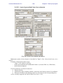
3.4. Data Input
3.4.1. Data Input Sequence
The following sequence of object data input is recommended.
1. Bodies, their graphical images and the corresponding joints.
The sequence of description of bodies is usually defined by the kinematical scheme of the
object. At first, the bodies connected with the base body (SC0) are described, and then the bodies
connected with already described bodies and so on. By such a description sequence of
kinematical scheme of object all its bodies are drawn not only in the current element animation
window but also in the whole object mode of the animation window (Sect. 3.3.1.2.2). It is
important to remember, that in the mode of whole object animation, the described body is drawn
in the animation window only if there exists a path from the current body to the base body
through the described joints.
2. Force elements and their graphical images
After describing the object kinematical scheme, force element images are drawn in the
animation window both in the current element and the full object animation mode, which allows
the user to control geometrical parameters of force elements visually.
Universal Mechanism 5.0
3-36
Chapter 3. Data input program
3.4.2. Input of subsystems
Subsystems are widely used for modeling of complex and specific mechanical systems. (see
Chapter 2, Sect. Subsystems).
There exist the following buttons:
– create a subsystem;
– copy an existing subsystem;
– delete a current subsystem.
There are three types of subsystems: included, external, and standard ones. Standard
subsystems are prepared subsystems, which are delivered together with additional modules of
UM and described in the corresponding part of user’s manual (for example subsystem
“wheelset” delivered and described in the railway module UM Loco). After choice of subsystem
type (included or external) user needs to open UM object which will be a subsystem in the
current object.
Fig. 3.27. Data inspector for subsystems.
Universal Mechanism 5.0
3-37
Chapter 3. Data input program
Main parameters of external and included subsystems are almost the same. They are name,
comment, position of the subsystem, identifiers used in the subsystem, and the identifier of the
subsystem used for programming. Also an external subsystem has one more parameter
Ancestor, which is the path to the folder with ancestor of the subsystem. To convert an external
subsystem to an included one click the button Convert to included on the tab General.
3.4.2.1.
Setting connection with external subsystems
Two methods can be used to connect bodies of different subsystems with joints or force
elements: 1) create necessary element (joint or force element) in the main object; 2) use external
bodies in subsystems (3.4.8.1). In the second method, it is necessary to point bodies and
characteristic points of these bodies for joints and force elements which use external bodies. For
that user should select the element Connections from the List of elements. The element
Connections is the list which contains all joints and force elements with the second body that is
external. Setting a connection means to point which body is external for considered element and
which point of this body is characteristic for the element. Double click checks the box on the left
of the element in the List of elements and opens the object tree where the lower level is the level
of connection points. Select the necessary connection point of the body. The connection is ready.
If it is needed to reset the connection uncheck the box of the element and use double click to set
it again.
Universal Mechanism 5.0
3.4.3.
3-38
Chapter 3. Data input program
Standard interface for setting local system of coordinates
B
r2
O
r1
A
Fig. 3.28 Setting position of local SC
The interface allows the user to define a fully parameterized position of a local system of
coordinates (LSC) relative to SC of a body, a graphic object or a graphic element. Consider a
SC with an origin in point O (SCO). It is necessary to define the position of SCВ relative to
SCO.
First, an auxiliary SC with the origin in point A (SCA) is introduced, which position
relative to SCO is set by the shift vector r1 and by a set of up to three sequential rotations.
After that the position of point B relative to SCA is specified by the vector r 2 . Thus, axis of
SCA and SCB are parallel. In particular case r 2 = 0 and SCB coincides with SCA.
The auxiliary SCA is sometimes useful when shifts could be specified simpler relative to
already rotated exes, i.e. relative to SCA.
Fig. 3.29 Window for specifying an LSC
The standard interface for setting LSC is shown in Fig. 3.29. Data are entered in three
groups.
- Translation. Projections of vector r1 in SCO are entered.
Universal Mechanism 5.0
3-39
Chapter 3. Data input program
- Rotation. Sequence of rotations specifies orientation of SCA and SCB relative to SCO. It is
allowed up to three rotations. Angles of rotation are set here in degrees.
- Shift after rotation. Projections of vector r 2 in SCA are entered, i.e. shifts along axes of
SCA.
Both projections of vectors and angles of rotation can be parameterized.
The interface is used for input of the following data types.
· Position of a graphic object (Sect. 3.4.6)
· Position of a graphic element relative to SC of graphic object (Sect. 3.4.6.4).
· Setting local SC for special force element of the “Bushing” type (Sect.
3.4.10.6.5).
· Setting local SC for scalar torques (Sect. 3.4.10.2).
· Setting local SC for 6 d.o.f. joint (Sect. 3.4.9.5).
Universal Mechanism 5.0
3-40
Chapter 3. Data input program
3.4.4. Assigning Graphical Image to Object Element
Graphical images (graphical objects, GOs) can be assigned to the most of UM elements, for
example, to the scene, bodies, some kinds of joints (e.g. a rod), some kinds of force elements
(bipolar, linear) and so on. Clicking a graphical image of element by mouse, the user can open
the element description in the object inspector. For this purpose the whole object animation mode
must be set in the animation window (Sect.3.3.1.2.2).
Graphical image is assigned to an object element from the list of the previously described
GOs using a drop-down list in the inspector of the current element (body, for example).
Fig. 3.30. Assignment of a GO
The drop-down list contains names of GOs, which have been set by the user while describing
graphical objects or by default. To make choosing GO easier, it is recommended to give sensible
names to GOs (Fig. 3.30).
Activate the corresponding drop-down list and press the Delete key to cancel the assignment
of a GO to the element.
There are some features by assigning GO to the object element.
GO can be assigned to each body; the same GO may correspond to several bodies (this is the
main principle). The GO system of coordinate is automatically superposed with the SC of the
corresponding body. All elements of mechanical system, which are fixed relative to the base SC0
(e.g. plane supporting a rolling ball, obstacles etc.), should be presented by a single GO, which is
assigned to the scene image (Common | Scene image inspector tab).
While drawing GO in the animation window, UM superposes the point (0,0,0) with the first
connection point (of the first interconnected body), and the point (0,0,1) with the second
connection point, at that UM properly changes the length and the orientation of the GO.
All elements (bodies, joints, force elements) having graphical image can be selected by the
mouse pointer in the animation window and then be accessed in the element inspector form. This
feature is very useful in cases if the object description contains many elements.
3.4.5. Assignment of graphic images to rods, linear and bipolar force
elements
A GO can also be assigned to a linear or bipolar force element (Sect. 3.4.10.2, 3.4.10.1) or to
a weightless rod constraint (Sect. 3.4.9.8). These elements link two points of different bodies.
UM automatically puts the assigned GO between the points. There is an obligatory condition
while creating such a GO:
A GO corresponding to a linear or bipolar force element or to a rod constraint must be
located along the Z axis of the SC GO between the points (0,0,0) and (0,0,1), that is the GO must
have the unit length.
3.4.6. Input of Graphical Objects
For description of graphical objects (GO), a built-in graphical editor is used. It is accessible
with the inspector tab Images. Notice that it is recommended to describe the rest of object
elements after the complete description of graphical images. In this case the visual verification of
input data is possible, and it allows avoiding a lot of input errors.
Universal Mechanism 5.0
3.4.6.1.
3-41
Chapter 3. Data input program
Lists of Graphical Objects and Graphical Elements
To visualize any system element (body, joint, force element and others; bodies will only be
mentioned below), it is necessary to assign a graphical object to it. GO is a set of graphical
elements (GEs), which should be created using the built-in graphical editor. The same GO may
belong to different (geometrically identical) bodies. For example, for description of GO of a
bogie having four similar wheels (even if their have different masses), it is enough to create two
GOs: a body and a wheel. The same wheel GO is assigned to each of the wheels.
It is desirable to create a full set of GOs before input of data for bodies, joints etc. In this
case the visual verification of input data is possible.
After assigning a GO to an object element, UM superposes the SC of GO with the element
SC in a certain rule, but it should be remembered, that the shape and sizes of GO are not
connected at all with inertia parameters of body, stiffness of spring and other parameters of the
object elements, which should be described separately. Exclusion presents the case when the
option for automatic calculation of body inertia parameters is turned on.
To go to describing (or changing) graphical objects or elements (GOs or GEs) use the
Graphical images tab, Fig. 3.11. The object inspector is shown in Fig. 3.31.
Fig. 3.31. Graphical object in the data inspector
On top of the inspector, tabs for graphical elements marked with their names are located. The
user can rename GOs using the corresponding edit box.
The current GO can be replaced from or stored in a text file using buttons
.
Each GO is a set (list) of graphical elements (GE), which is shown a bit below. Lower
buttons
are intended for:
· adding a new GE;
· copying (duplicating) the current GE;
· deleting the current GE.
Universal Mechanism 5.0
3-42
Chapter 3. Data input program
To set (change) the type of the current GE a drop-down box is used, which contains names of
the standard GEs:
· polyhedron;
· ellipse;
· box;
· spiral;
· ellipsoid;
· cone;
· parametrical GE;
· profile GE;
· Z-surface.
While describing almost all parameters of GEs, identifiers and symbolic expressions may be
used.
Remark. Changing a type deletes previously entered data for the current GE.
3.4.6.2.
Input of graphical elements (GE)
Each GE has four groups of parameters located in the different tabs (Fig. 3.31):
· Parameters – a tab with GE parameters depending on its type;
· Colors – a tab with GE color information;
· Position – a tab with parameters describing position and orientation of the current GE in
the SC of the current GO;
· Material – parameters defining inertia properties of the GE material (such as density).
They are used for automatic calculation of inertia parameters of bodies.
3.4.6.2.1.
Polyhedron
A polyhedron is used when a GE of irregular shape is needed. An UM polyhedron is a set of
3D vertices forming one or more polygons. The polygons may be drawn both in line and filled
modes.
To describe a polyhedron the following parameters should be set (Fig. 3.32):
· Coordinates of vertices. If only vertices are given then the result is a single broken line
formed with these vertices. But if several polygons are needed then the lower part of the
form shown in (Fig. 3.32) is to be filled:
· For each polygon, vertex indices delimited with commas should be pointed; filled
polygons should be marked with .
Universal Mechanism 5.0
3-43
Chapter 3. Data input program
Fig. 3.32. Polyhedron
Example. Four vertices might set a tetrahedron
(0 0,0), (1,0,0), (0,1,0), (0,0,1)
and four polygons
(1,2,4), (4,2,3), (1,4,3), (1,3,2).
3.4.6.2.2.
Ellipse
Parameters of an ellipse (Fig. 3.31):
· a, b – semi-axes;
· starting and ending angles (for a elliptic sector). Default values (0,0) correspond to a full
ellipse;
· discretization is the number of points approximating the ellipse;
· filled option determines the element either as plane or a line.
3.4.6.2.3.
Box
All ribs of a box are parallel to the axes of the GE-fixed SC. The box parameters are
Fig. 3.33. Box parameters
Universal Mechanism 5.0
·
·
3-44
Chapter 3. Data input program
Length, width, height A, B, C (constant symbolic expressions);
Discretization (0..4) specifies the number of finite elements on a box side (about 2n
elements on each side) in the line mode.
3.4.6.2.4.
Spiral
This GE is used customarily as to draw elastic linear of bipolar force elements. The spiral
parameters are (Fig. 3.34):
· coil radius r (a constant symbolic expression);
· spring height H (a constant symbolic expression);
· the number of coils;
· coil discretization.
Fig. 3.34. Parameters of a spiral
The axis of the spiral coincides with the z-axis of the GE-fixed SC.
3.4.6.2.5.
Ellipsoid
This GE allows showing an ellipsoid or, particularly, a sphere (Fig. 3.35).
Fig. 3.35. Parameters of an ellipsoid
The parameters of an ellipsoid are:
· a, b, c – its semi-axes;
· Slices, Stacks – number of points to approximate the ellipsoidal surface.
The center of the ellipsoid is placed into the begin of the GE SC.
Universal Mechanism 5.0
3.4.6.2.6.
3-45
Chapter 3. Data input program
Cone
The dialog form for input of a cone is shown in Fig. 3.36.
Fig. 3.36. Cone
The GE allows getting such images as cylinder, cone and truncated cone, also only a part of
these surfaces.
For description of conic surface the user should input the parameters:
· R1, R2 – radii of the upper and bottom circle-bases;
· h – height of cone;
· Angles – starting and finishing angles (in degrees) that form a plate angle at the Z-axis,
which delimits the conic surface. The angles are counted from the X-axis
counterclockwise. In case if both angles are zeros then the full cone (cylinder) is
generated;
· Number of points on the circle bases and the generating line, which define a
discretization of the conic surface;
· Closing – this switch has three positions (None), Sector, Segment and defines how the
conical surface should be closed.
3.4.6.2.7.
Parametrical GE
The GE provides the wide possibilities to describe the complex surface as analytical surface
in a parametric form (Fig. 3.37). Description of 3D curves and surfaces is allowed. The user
should describe them as arbitrary functions of a single (p1 or p2) or the two parameters (p1 and
p2).
Universal Mechanism 5.0
3-46
Chapter 3. Data input program
Fig. 3.37. Parametrical GE
The parameters of the parametrical GE are
· Standard – there are a set of standard parametrical elements:
Plane
Ellipsoid
Ring
Torus
Cone
Paraboloid
Spring
Horn
Molecule (Fig. 3.37)
Smooth cube
Gear
Elliptic gear
· Equation – analytical expressions describing the dependence of the Cartesian
coordinates X, Y and Z on a parameter p1 or p2 (for a 3D curve), or p1 and p2 (for a 3D
surface);
· Parameter limits – for each parameter, the minimal and the maximal values should be
given, and the number of points inside the interval to approximate the surface, too; for
example, the values p1 from –1.4 to +1.2, p2 from –0.2 to 4.8 modify the surface above
as shown in Fig. 3.38.
Fig. 3.38. Influence of the parameters p1, p2 on the GE shape
·
Closing – there is a possibility to complete the surface to the closed one by adding lids;
since the parameters p1 and p2 are equivalent, so a lid can be treated either as the
p1=const or as the p2=const surfaces (Fig. 3.39); for this purpose the corresponding
switch is intended (Fig. 3.37).
Universal Mechanism 5.0
3-47
Chapter 3. Data input program
Fig. 3.39. Different ways of making the parametric GE closed
3.4.6.2.8.
Profiled GE
This GE has many possibilities. It defines a surface formed by moving a certain profile curve
along another axis curve, a number of ways to build the curves being possible.
Fig. 3.40. Profiled GE: a cylinder
An example of the profiled GE is shown in Fig. 3.40.
Parameters of the profile are:
· Type of section – possible values are:
- Circle: semi-axes are Scale X, Scale Y;
- Curve 2D: a section given by a number of points, holes are allowed, too;
- Spline 3D:a set of consecutive sections given by points;
- Expression:
a section given by analytical formulas.
· Scale X, Scale Y – scales in X and Y axes;
· Number of points to approximate the section;
· Close – a switch for automatic adding lids to make the surface closed.
Parameters of the axis curve are:
· Type of curve – possible values are:
- Straight line;
- Circle;
- Curve: given by points;
- Expression: given by analytical formulas.
· Length – the length of the axial line (in case of straight axis curve);
· Number of points to approximate the axial curve.
Universal Mechanism 5.0
3-48
Chapter 3. Data input program
Using various combinations «type of profile curve – type of axis curve», it is possible to get
different shapes of GE.
Examples of profiled elements
After choosing the profile type Curve 2D or Curve 3D, a new input parameter Description
appears (Fig. 3.41).
Fig. 3.41. Profiled GE: a Curve 2D section
Clicking mouse button on
, the user can open a window of the curve editor
(see Sect. 3.4.6.6) and input the section.
If several curves are presented with the Curve 2D type then the profile section will be
multiple connected (Fig. 3.41).
In case of the Curve 3D section type, several curves are treated as a set of consecutive
sections along the axis curve (Fig. 3.42).
Fig. 3.42. Profiled GE: a Curve 3D section
After choosing the Expression type of profile section, a new parameter group
appears (Fig. 3.43):
· x(p), y(p) – parametric equations of the profile contour depending on p;
· Pmin, Pmax – limits of changing p.
Universal Mechanism 5.0
3-49
Chapter 3. Data input program
Fig. 3.43. Profiled GE: section given by formulas
Analogously, the axis curve can be described by points (Fig. 3.44).
Fig. 3.44. Profiled GE: a 2D axis curve given by points
3.4.6.2.9.
Z-surface
A GE of this kind is intended for programming graphical image of an arbitrary surface in the
control file. The surface should be described as
z = f ( x, y ) ,
where x and y coordinates correspond to parameters p1, p2.
Universal Mechanism 5.0
3-50
Chapter 3. Data input program
Fig. 3.45. Z-surface parameters
The GE description includes
· name of function;
· parameter ranges – limits of changing both p1 and p2 parameters and numbers of
pointes to approximate the surface.
When generating equations of motion, a template for zSurface function is included in the
control file (for example, as Pascal code):
function ZGraphicElementFunctions(
_index, _isubs : integer;
_p1, _p2 : real_ ) : real_;
begin
_ := _PzAll[SubIndx[_isubs]];
case _index of
0 : begin
{ Function zSurface }
Result := 0;
end;
end;
end;
For each function of type Z-surface introduced for representation of graphical images, an
operator Result := 0 is inserted, and the user should replace it with a proper calculation.
GE of type Z-surface is used to represent images with the help of complex implicit functional
expressions, including time-dependent ones. For example, the Z-surface was used to get a
traveling wave (Fig. 3.46).
Fig. 3.46. Z-surface
Universal Mechanism 5.0
3-51
Chapter 3. Data input program
More detailed information concerning this GE is discussed in the manual for programming in
UM environment.
Remark. Since the real description of the GE is located in the control file and is accessible in
the UM Simulation program only, so in the input program the element is showed as a rectangle
of sizes defined by change limits of parameters p1, p2.
3.4.6.2.10.
GO as a graphic element
A previously created GO can be included in the current GO as a graphic element (type GO of
the graphic element). This feature allows the user to create a many time repeating group of
graphic elements as a separate GO and insert it several times in another GO. After that the
correction of included GO leads to modification of all the GE-GO.
For example, consider an image of a fright couch body. It includes a lot of repeating parts
(stiffening ribs) one of which is selected in the picture (Fig. 3.47). It should be created a GO
corresponding to a separate rib and then this image is dozens of times included in the image of
the body as GE-GO and positioned by a proper way. If the image of the rib must be modified
(e.g. its height must be reduced), the only GO of the rib should be corrected, and all the ribs
included in the image of the coach body are changed automatically.
Fig. 3.47. Graphic image of a fright couch body
Universal Mechanism 5.0
3.4.6.3.
3-52
Chapter 3. Data input program
GE colors
Colors of a GE are set by parameters on the tab Color (Fig. 3.48).
Fig. 3.48. Colors of GE
There are several kinds of colors:
· Diffuse (color of material);
· Specular (color of the reflected light); black color means no reflection;
· Emissive (the object shines with this color); it is off if the color is black;
· Ambient (usually not used).
To choose each of the colors click mouse button on the corresponding color rectangle.
Use the
button to select one of the standard color sets.
The parameter Shininess defines size of the reflected light’s spot.
Check the Wired option to convert the element into the wire mode; simultaneously the
Width of curves parameter set the line width.
Universal Mechanism 5.0
3.4.6.4.
3-53
Chapter 3. Data input program
Position and Orientation of GE
Fig. 3.49. Position and orientation of GE
Each GE contained in GO is described in its own system of coordinates – SC GE, which can
be positioned in SC GO in an arbitrary way – it can be turned through some angles about the
three axes in an arbitrary order and can be translated. Rotation angles are given in degrees,
rotation axes being chosen previously.
Universal Mechanism 5.0
3.4.6.5.
3-54
Chapter 3. Data input program
Inertia parameters of GE
Fig. 3.50. Inertia parameters of GE material
Inertia parameters of bodies (mass, tensor of inertia, coordinates of center of mass) can be
computed automatically according to the body image. A necessary condition for that is filling the
material properties for graphic elements (at least for one of them). On the Material tab (Fig.
3.50) set
· Density
· Type of graphic element (solid, hollow) or frame (for wire element, Sect.3.4.6.3)
· A thickness and a section square should be set for a hollow and a wire GE
Warning. Automatic computing of inertia parameters may lead to wrong results if separate
graphic elements intersect. The intersected volumes are taken into account several times. For
example, the mass of the body is computed according to the formula
m = å mi
where mi is the mass of a separate GE calculated independently on possible intersections.
Universal Mechanism 5.0
3.4.6.6.
3-55
Chapter 3. Data input program
Curve editor
The window of the curve editor is shown in Fig. 3.51. See Sect.3.3.3 for basic information
about this tool.
Fig. 3.51. Curve editor
Main elements of the editor are marked by indices:
· graphical primitives:
1 – straight lines;
2 – cubic splines;
3 – beta-splines (special kind of splines);
4 – circle (arc);
· points (vertices):
5 – a point of smooth conjugation of primitives;
6 – a point of non-smooth (sharp) conjugation of primitives;
· continuous curves (continuums):
1-5-2-6-2-1-4-1, and also 3 – non-closed curves;
4, 7 – closed curves;
· other controls and possibilities of the editor:
8 – drop-down list of types of primitives;
9 – selection of a group of primitives by means of the mouse;
10 – panel of control buttons;
11 – list of curves;
12 – grid with coordinates and parameters of the current (selected) curve.
For adding points (vertices), double clicking the left mouse button is using.
To copy (duplicate) a curve:
· select it using mouse pointer;
· put it to the Windows clipboard;
· insert from the clipboard.
Universal Mechanism 5.0
3-56
Chapter 3. Data input program
Exchange with the clipboard is performed using a text format. So, the user can type
coordinates of vertices as two columns of numbers in any text editor, and insert them into the
curve editor.
Pop-up menus are used for various actions with primitives and points of curves. It appears
after clicking the right mouse button over the corresponding element.
For example, clicking over the free field of the curve editor results in appearing a pop-up
menu shown in Fig. 3.52.
Fig. 3.52. Curve editor main pop-up menu
The menu has two items:
· Start new curve – the next point being input will be the start point of the new curve
(continuum);
· Select all – is used to select all curves in the editor.
Clicking right mouse button over any vertex results in appearing a pop-up menu for a point
(Fig. 3.53).
Fig. 3.53. Pop-up menu for a point
Actions allowed for a selected point are:
· Properties... – opens a point property dialog box intended for changing the point
coordinates;
· Delete – removes the selected point;
· Smooth – turns on/off the smooth conjugation of primitives.
A pop-up menu for a primitive appears after clicking any primitive (line, spline or circle); see
Fig. 3.54.
Fig. 3.54. Pop-up menu for primitive
Actions allowed for a primitive are:
· Convert into – changes the type of the selected primitive;
· Insert point – a new point will have the coordinates defined by the current position of
the mouse pointer (double clicking the left mouse button has the same effect);
· Delete – removes the selected primitive;
· Properties... – calls a primitive property dialog box;
Universal Mechanism 5.0
·
·
·
·
3-57
Chapter 3. Data input program
Select whole curve – selects the curve (continuum) containing the selected primitive;
Closed – a tag for closing the curve containing the selected primitive;
Reverse order – for inverting the ordering of points;
Rotate 90 – turns the current continuum through 90 degrees counterclockwise.
Universal Mechanism 5.0
3-58
Chapter 3. Data input program
3.4.7. Input of bodies
Fig. 3.55. Bodies item of the object element list and Body parameters
The Bodies item of the object element list (Fig. 3.55 left, Sect.3.3.2.1) is used for access to
procedures of creation and modification of the list of bodies and their parameters. Alternative
ways are the Ctrl+Alt+B hot key or clicking by the mouse on the corresponding body image in
the whole object mode of the animation window (Sect.3.3.1.2.2). The right picture in Fig. 3.55
shows the inspector with parameters of a body.
Universal Mechanism 5.0
3.4.7.1.
3-59
Chapter 3. Data input program
Image and visualization of a body. Body-fixed SC
The Graphic image pull-down list contains all entered graphical objects (see Sect. 3.4.2).
Click the
button to access the assigned GO parameters or to create a new GO, which will be
assigned to the body.
The SC of the assigned GO coincides with the body-fixed SC. That is why the image moves
when the body changes its position and orientation.
Use the single element mode of the animation window (Sect.3.3.1.2.2) to see the body-fixed
SC and the body image.
a)
b)
c)
Fig. 3.56. Visualization of an active body in different modes of the animation window
Fig. 3.56 shows visualization of a motor body in different modes of the animation window:
a) Full object mode, the active body is drawn as selected, axes of the SC0 are drown
b) Single element mode, the window contains the body image in the body-fixed SC
which axes are drawn
c) Single element mode, wire graphics
Important remark. A body is drawn in the full object mode of the animation window if
there exists a path from the body to the Base0 through the joints (Chapt. 2, Sect. Compendency
of systems and the definition of a joint). For example, if body2 is connected to body1 and body1
is connected to Base0 by means of two rotational joints, both body1 and body2 are visible in the
full object mode. If the joint between body1 and Base0 is removed, both bodies disappear. If the
joint between body2 and body1 is removed, body1 disappears.
Universal Mechanism 5.0
3.4.7.2.
3-60
Chapter 3. Data input program
Inertia parameters
Inertia parameters of a body are:
· mass;
· symmetric inertia tensor;
· coordinates of center of mass in the body-fixed SC;
· symmetric added mass matrix.
The icon
marks the position of the center of mass in the animation window.
Important remark and warning. Moments of inertia and elements of the added mass matrix
should be calculated in SC, which origin coincides with the center of mass and axes are parallel
to those of the body-fixed SC.
There exist two modes for entering the inertia parameters (except the added masses). Use the
Automatic calculation button to switch them. (Fig. 3.55).
User’s defined inertia parameters
All parameter boxes are enabled in this mode. All parameters might be constant symbolic
expressions (Sect.0).
Automatic calculation of inertia parameters
The parameters are calculated automatically according to the body image (Sect.3.4.6.5).
Parameter boxes are not available for the user.
Remarks.
· Automatic calculation is enabled after assigning a GO to the body. The corresponding
GO must include at least one GE with the assigned material which density is not zero.
· Inertia parameters are recalculated every time when the GO is modified in particular
when identifiers parameterizing the GO are changed.
3.4.7.3.
Adjust/adjusted joint
Use the button to create or modify an adjusted joint for the current body (Sect.3.4.9).
The adjusted joint is the nearest joint, which lies on the path from the body to the base. Use
this joint to change the position of the body.
3.4.7.4.
Connection points
Connection points are assigned to the body. They are used by
· operations with visual components;
· describing joints and force elements (visual assignment of bodies, joint and attachments
points);
· assignment of bodies as will as the corresponding joint and attachment points to external
joint and force elements (for subsystem technique only).
There exist three types of connection points:
· general
· oriented (local body-fixed SC)
· vectors
Universal Mechanism 5.0
3-61
Chapter 3. Data input program
The following parameters should be set for each point
· coordinates in the body-fixed SC (coordinates are parameterized);
· comments simplifying operations with points (auxiliary parameter);
· orientation of point-fixed SC relative to the body-fixed SC (for oriented point); the
orientation is set by three rotations.
An icon marks a connection point in the animation window (Fig. 3.57). A point-fixed SC
are additionally drawn for oriented points, and a line section is drawn for a vector along its
direction.
Fig. 3.57. Frame with general and oriented connection points
Note.
Connection points are used to assign their positions and/or orientation to object elements
(joints and forces). At the same time the connection between the element and the points is not
kept. This means that if the user changes the point parameters after its usage for description of an
element, the corresponding changes are not transferred to the element automatically.
3.4.7.4.1.
Tools for list
modification
Adding general connection points
Tools for visual
creation of points
List of points
The Points tab is used to create or modify the list of points.
To add a point, the user should set its coordinates in the body-fixed SC. Here are instructions
how to do this.
1. Use the
(add) or the
(copy) button. Set point coordinates as constant symbolic
expressions, Sect. 0.
2. Click the
button, select by the mouse a point on the body image, and click the mouse
button again. The selected point is added automatically.
Universal Mechanism 5.0
3-62
Chapter 3. Data input program
Second click
Result
First click
Selection of
image vertex
Adding a point as a middle point of a section
3.
The ( ) button allows the user to get a point as a middle point of a section selected by the
mouse.
Use vertices on the body image for exact positioning of points. Near the vertex the mouse
cursor is changed to . After visual adding, the point can be corrected or removed by the
button.
3.4.7.4.2.
Adding oriented connection points
Use the Oriented points tab to add an oriented connection points (a local system of
coordinates, LSC). Its description includes coordinates of the points and the orientation of axes
of the LSC in the body-fixed SC. The orientation is set as a sequence of tree successive
elementary rotations.
Here five methods for adding oriented points (LSC) are described.
1.
(add) or the
(copy) button. Set point coordinates as constant symbolic
Use the
expressions, Sect. 0. Set rotation axes and angles in degrees to define the orientation.
Universal Mechanism 5.0
3-63
Chapter 3. Data input program
Adding a LSC by a normal and a point
2.
Visual adding by a normal and a point.
· Click the
button.
· Select a vector or a point on a plane for the origin and the Z-axis of the LSC.
· Select a point in the XZ-plane.
3. Visual adding by an opposite normal and a point.
·
·
·
Click the
button.
Select a vector or a point on a plane for the origin and the Z-axis of the LSC. The Z-axis
is directed opposite to the vector or inside the plane surface.
Select a point on the XZ-plane.
Visual adding a LSC by tree and by four points
4.
Visual adding by three points.
· Click the
button.
· Select a point for the origin of the LSC.
· Select a point on the X-axis.
· Select a point in the XY-plane.
5. Visual adding by four points.
·
Click the
button.
Universal Mechanism 5.0
·
·
3-64
Chapter 3. Data input program
Select two points. The middle point of the section is the origin of the LSC, and the vector
r12 connecting the points set the X-axis.
Select the 3rd and the 4th points. The cross product r12 ´ r34 sets the Z-axis.
3.4.7.4.3.
Adding vectors
Fig. 3.58.
Use the Vectors tab to add a vector. Its description includes coordinates of the points and
components defining the direction of the unit vector in the body-fixed SC. The vectors are used
for visual correction and adding joints and some special force elements.
1.
2.
3.
4.
5.
6.
Here five methods for adding vectors are described.
Use the
(add) or the
(copy) button. Set point coordinates as constant symbolic
expressions, Sect. 0. Set numeric values for the vector components.
Visual adding by a normal and a point.
· Click the
button.
· Select a point on a plane for the vector, which is the external normal to the plane.
Visual adding by two points.
· Click the button.
· Select a point for the vector point.
· Select the second point for the vector direction.
Visual adding by three points.
o Click the
button.
· Repeat actions for setting the LSC by three points from the previous section. The vector
corresponds to the Z-axis.
Visual adding by four points.
· Click the
button.
· Repeat actions for setting the LSC by four points from the previous section. The vector
corresponds to the Z-axis.
Visual adding as a normal to the center of a circle passing through 3 points.
· Click the
button.
· Select three points lying on a circle. The resulting vector begins at the circle center. The
direction of the vector is perpendicular to the circle plane according to the right-hand
screw rule according to sequence of selected points.
Universal Mechanism 5.0
3.4.7.5.
3-65
Chapter 3. Data input program
3D Contact
There is a possibility to assign a contact manifold described as a graphical object
(see. Sect. 3.4.6. Input of Graphical Objects, page 3-40) to a rigid body. All bodies that have
such a contact manifold will interact between each other during simulation dynamics of a
mechanical system in UM Simulation. Parameters of a contact interaction as well as turning
on/off contact between pairs of bodies are available in UM Simulation.
3D Contact supports parameterization of graphical objects that are used as contact manifolds.
Firstly parameterized graphical objects for contact manifolds you can consider various
configuration of contacting bodies in quite wide range simply changing corresponding
parameters without remaking the graphical object itself. Parameterization of graphical object
may be effectively used, for example, for searching the optimal shape of the friction wedge for
so-called three-piece bogie for freight cars, Fig. 3.59 below.
a) Graphical object (GO)
b) Contact manifold (CM)
c) GO and CM
Fig. 3.59. Graphical object and contact manifold for a body of wheeled robot
A graphical object that is assigned as a contact manifold for a body may differ from a
graphical for the body. It is absolutely not necessary that it should be the same graphical objects.
It is recommended to use simplified contact manifolds for decreasing the CPU efforts for
simulation.
The contact manifold for the rigid body is selected from prepared in advance graphical
objects that are available in the drop down list. Coordinate system of the contact manifold
coincides with the coordinate system of the body. In the Single element mode (see
Sect. 3.3.1.2.2. Modes of animation window, page 3-15) the contact manifold is drawn in yellow
lines, see Fig. 3.60.
There is no possibility to assign a contact manifold for Base0 body. If it is necessary you
should create an extra rigid body with 0 d.o.f. and assign the contact manifold of Base0 with this
extra body.
Universal Mechanism 5.0
3-66
Chapter 3. Data input program
Fig. 3.60. 3D Contact parameters between pair of bodies
Types of contact manifold
Polyhedron. In general case use Polyhedron type for describing the contact interaction
between bodies. Graphical objects that are chosen as contact manifolds should consist of
graphical elements of the following types: Box, Polyhedron and ASC. Graphical elements of
Polyhedron and ASC types should be convex and closed.
Z-surface. This type of contact manifold is used to describe contact between all bodies and
the ground. Restrictions of convexity and closure are not applied for graphical objects for contact
manifold of Z-surface type. Some comments concerning preparing a graphical object for using
as a contact manifold of Z-surface type are given in Sect. 3.4.10.4.5. Points / Sphere / Circle - Z
surface contact, page 3-100.
3D Contact simulation between Polyhedrons and Z-surface is based on using Points –
Z-surface contact force that is described in Sect. 3.4.10.4.5. That is why it is also possible to
describe contact interaction between polyhedrons and Z-surface with the help of Points –
Z-surface contact force. The only difference between both variants is that 3D Contact generates
all contact forces of Points – Z-surface type automatically without necessity to create the forces
for each body and the Z-surface manually. At the same time both variants are identical from
point of view of results of simulation of dynamics of the system.
Treating the Points – Z-surface contact forces in 3D Contact does not consider the
interaction of edges and Z-surfaces, so contact forces will not appear in the case which is
depicted in the Figure below.
Polyhedron
Vertex
Z-surface
Universal Mechanism 5.0
3-67
Chapter 3. Data input program
Note 1. CPU efforts for simulation of near contact are proportional to square of count of
faces and edges. To accelerate simulation process it is recommended to simplify contact
manifolds 1 as far as possible for solving the particular problem.
Note 2. 3D Contact model as any mathematical model is just an approximation of real physical
processes that take place between two bodies contacting bodies. Certainly the model has confined
area of effective applications as well as there are cases where the model describes real processes
incorrectly. 3D Contact model is rather a fast algorithm that is suitable for simulation of some
models based on multibody system dynamics approach but surely is not suitable for detailed
analysis of contact problem (contact stresses, deformations, wear, plastic effects and so on).
Comparison of the contact models.
Universal Mechanism software has to approaches to simulate contact interaction between
rigid bodies. The first approach suppose using contact forces of “point-plane” and other types
and the second approach is based on 3D Contact described above.
3D Contact based on using “point-plane” contact forces and in this sense can be considered
as an algorithm that detecting interpenetration of rigid bodies arranges contact points and
identifies nearest faces as contact planes. At the same time calculation of interpenetration of
contact manifolds is rather time-consuming operation that takes quite many CPU efforts. That is
why simulating models with contacts it necessary to understand clearly advantages and
disadvantages of both approaches. Detailed overview of contact forces see in Sect. 3.4.10.4.
Input of contact force elements, page 3-97.
3D Contact often makes simulation of contact interaction more easy-to-use, intuitive and
more suitable for parameterization, as well as widens contact interaction for “edge-edge”
penetration case, see Chapter 2, Sect. 3D contact. To simulate “edge-edge” penetration with the
help of contact forces of “point-plane” type it needs to create contact points on each edge with
quite small distance between them that significantly increases CPU efforts that neglect the only
benefit in comparison with 3D Contact.
Please note that 3D Contact widens possibilities of simulation of contact interactions but
needs extra computational efforts. At the same time approach based on using contact forces
generally faster but not so universal as 3D Contact one.
Examples.
Please find some examples of using 3D Contact in the following models:
· ..\Samples\Misc\Clockwork;
· ..\Samples\Misc\DominoDay;
· ..\Samples\Misc\Earthquake;
· ..\Samples\Misc\FallingFigures;
· ..\Samples\Rail vehicles\WedgeTest3DContact;
· ..\Samples\Robots\Manipulator;
· ..\Samples\Robots\krt_200.
Universal Mechanism 5.0
3-68
Chapter 3. Data input program
3.4.8. Joints and force elements: some features of description
Joint and force elements have some parameters, which entering is quite analogous, e.g. a pair
of bodies, attachment points or images should be assigned for the most of elements of these
types. The standard interface is used for entering these parameters, for instance the
corresponding interface for a 6 d.o.f. joint looks like this (Fig. 3.61):
Body1
Body2
Element
type
Image
Attachment point
to Body1
Attachment point
to Body2
Fig. 3.61.
3.4.8.1.
Assignment of bodies
A pair of bodies should be assigned for each joint or force element else the object description
is considered as incomplete. One of the bodies is the first one (Body 1 in Fig. 3.61), another – the
second one (Body 2). Use two upper drop-down lists to set the bodies (Fig. 3.62).
Fig. 3.62
The lists contain all bodies included in the object as well as the base body (Base0) and an
external body (the second list only). The Base0 is used for attachment of a body to a fixed point
(to the base). The External body is used to make the element external (the subsystem technique).
The first and the second bodies must be different.
3.4.8.2.
Type of element
A type must be chosen for the most of elements with the help of a drop-down list (Fig. 3.61,
Fig. 3.63). Changing the type leads to deleting of previous element description.
Universal Mechanism 5.0
3-69
Chapter 3. Data input program
Fig. 3.63
3.4.8.3.
Attachment points
Attachment points have different notations for elements of different types (‘joint points’,
‘attachment point’ etc.). Anyway two points should be assigned for each element. One of the
points belongs to the first body, another point – to the second one. The coordinates of the point
should be entered in SC of the corresponding body as constant symbolic expressions
(Sect. 0).
3.4.8.4.
Visual assignment of bodies and attachment points
To assign visually a body and the corresponding attachment point click one of the
buttons
and select a point, an oriented point or a vector, which should be preliminarily described (see
Sect. 3.4.7.4. Connection points).
Note 1. The type of the point should be chosen depending on the element. For example,
description of a generalized linear force element requires both oriented points and general point.
The description of a bipolar force element requires two general points.
Note 2. If the element requires coordinates of a point only, all types of connection points can
be used. If the element requires a vector, an oriented point can be used (Z-axis of the LSC is used
as the vector).
3.4.8.5.
Transformation of coordinates
Attachment points of force elements are set in body-fixed SC, that is why, a tool for
transformation of coordinates of points into different SC could be useful. To call the
corresponding tool use the Tools | Transformation of coordinates ore use the hot key Alt+T
(Fig. 3.64).
Choose two bodies with the help of drop-down lists and set coordinates of a point in SC of
one of the bodies (where the coordinates are known). After that click either the
button (if the
coordinates are known for the first body) or the
button if the coordinates are known for the
second body), and the coordinates are computed for SC of another body. Analogously can be
computed projections of a vector onto axes of different SC.
Fig. 3.64. Example of transformation of coordinates
Universal Mechanism 5.0
3-70
Chapter 3. Data input program
3.4.9. Input of joints
3.4.9.1.
Visualization of joints
In the single element mode of the animation window: a pair of bodies (kinematical pair)
connected by the joint is drawn. A GO may be assigned for a rod constraint only.
In the full object mode of the animation window: the bodies of the kinematical pair are
drawn as active. Optionally an icon marks a position of the joint point and visualizes its degrees
of freedom (Sect. 3.3.1.2.1. Visualization of object elements). Click near the active region of the
icon to call the description of the joint in the inspector (Sect. 3.3.1.2.1).
If the joint is cut (except rod, mate and CV joints), the second body is drawn twice in the full
object mode: in the positions determined by adjusted and the cut joints (Sect. 3.4.9.1). It is
recommended to change coordinate values in such a way that the both images of the body were
close. The exact values of the coordinates are calculated in the Simulation program.
Note. By default some information about the joint is hidden. Use the
button to make it
visible.
3.4.9.2.
Weight of joint
Fig. 3.65. Setting joint weight
A weight coefficient can be assigned to each of the joints. This parameter is used when the
object has closed kinematical loops (Chapt.2, Sect. System graph. Closed kinematical loops). If a
large weight (e.g. 1000) is assigned to a joint in a closed loop, it will be cut.
Note. By default the weight information is hidden. Use the
button to make it visible, Fig.
3.65.
3.4.9.3.
Convertion of joint type
Joints of types
· rotational
· translational
· six degrees of freedom (6 d.o.f.)
can be converted to the “generalized” joint type.
For example, a 6 d.o.f. joint can be converted to the generalized type to introduce joint
forces for some degrees of freedom. A rotational or a translational joints is recommended to be
transformed to the generalized joint type, e.g. to add degrees of freedom or to parameterize
inclination of the joint axis.
To convert the joint type
- use the button to open additional joint information, Fig. 3.65.
-
click the
button to make the conversion.
Universal Mechanism 5.0
3-71
Chapter 3. Data input program
Example. User’s manual, Chapt. 7, Sect. Joint type conversion. Parameterization of axis
inclination.
Universal Mechanism 5.0
3.4.9.4.
3-72
Chapter 3. Data input program
Input of rotational and translational joints
Fig. 3.66. Parameters of a rotational joint
Notions of translational and rotational joints are discussed in Chapter 2, Sect. Translational
and rotational joints.
The following parameters should be entered in addition to bodies and joint points
(Sect. 3.4.8.1, 3.4.8.3):
· projections of the joint vector on axes of two body-fixed SC (the Geometry tab, Fig.
3.66); the vector cannot be zero;
· additional shift and rotation (the Description tab, the Configuration group); the
parameters are optional.
If the bodies connected by the joint are is in the tree (visible in the full object mode of the
animation window, set the
button in the ‘down’ state to verify this), the
buttons can be
used for visual entering both the joint points and the joint vectors. A joint vectors can be
obtained from connection points of vector and oriented point types (see Sect. 3.4.8.4. Visual
assignment of bodies and attachment points). Thus, selection of a vector or an oriented point
allows the user to assign simultaneously: a body, a joint point and a joint vector.
Further description of joint depends on type of the joint coordinate. The coordinate can be a
degree of freedom or a time function.
Coordinate is a degree of freedom
All parameters are optional:
· value of the coordinate – the box is usually used to verify the correctness of the joint
description: stepwise changing of the value leads to motion of bodies;
· type of the joint force/torque (Chapter 2, Sect. Joint forces and torques) can be chosen
from the drop-down list (Fig. 3.67) on the Joint force tab.
Universal Mechanism 5.0
3-73
Chapter 3. Data input program
Fig. 3.67. Types of joint force
After the type has been chosen, the boxes for force parameters appear.
Some features of description of the force/torque see in
Linear, Sect. Linear force element
Frictional, Sect. Friction and elastic-frictional elements
Elastic-friction, Sect. Friction and elastic-frictional elements
Elastic-friction 2, Sect. Elastic-frictional element 2
Viscous-elastic, Sect. Viscous-elastic element
Points (numeric), Sect. Points (numbers)
Points (express.), Sect. Points (expressions)
Expression, Sect. Expression – explicit function
External function, Sect. External functions
List of forces, Sect. Fancher leaf spring
Coordinate is a time function
Use the Prescribed time function check box to set this type of the coordinate.
Fig. 3.68. Time function
The time function can be set as
· an explicit expression (Sect. 3.3.2.4.5)
· an external function (Sect. 3.3.2.4.6)
· a time table (Sect. 3.3.2.4.9)
· a function from a text file (Sect. 3.3.2.4.8)
Remark. Both rotational and translational joints is recommended to be transformed to
the generalized joint type, e.g. to add degrees of freedom or to parameterize inclination of the
joint axis, Sect. 3.4.9.3.
Example. User’s manual, Chapt. 7, Sect. Joint type conversion. Parameterization of axis
inclination.
Universal Mechanism 5.0
3.4.9.5.
3-74
Chapter 3. Data input program
Input of 6 d.o.f. joint
Detailed description of the joint can be found in Sect. Chapt.2, Sect. Six d.o.f. joint.
Fig. 3.69. Description of 6 d.o.f. joint
In addition to connected bodies (Sect. Sect. 3.4.8.1), the user should set positions of local
joint system of coordinates SC1A and SC2B relative to SC1 and SC2 in the Geometry tab. For
this purpose the sheets Body1 and Body2 are used, Fig. 3.69 left. The standard interface is used
for parametric setting the SC positions, see Sect. 3.4.3.
The following parameters should be entered to specify the joint coordinates (Fig. 3.69, right):
· type of orientation angles;
· “turned on” degrees of freedom (check the presented degrees of freedom and turn off the
others); the three upper rows correspond to translational d.o.f. (Fig. 3.69).
Use the buttons ­¯ in the edit boxes to set initial values as well as to verify the correctness of
the joint description.
Remark 1. Cut joints with six d.o.f. are ignored in the Simulation program.
Remark 2. 6 d.o.f. joint can be converted to the generalized type to introduce joint forces
for some degrees of freedom, Sect. 3.4.9.3.
Example. An example of a joint used for setting six degrees of freedom of a box relative
to SC0 according to data in Fig. 3.69 left for x0=1m, alpha=30 degrees is shown in Fig. 3.70.
The box is shown in the position corresponding to zero values of joint coordinates. Features of
the joint are the parametric description of both the SC1A origin (shift along the X-axis x0) and
angle of rotation about the X axis (alpha). As a result two translational and two rotational
degrees are specified along inclines axes Y and Z.
Universal Mechanism 5.0
3-75
Chapter 3. Data input program
Fig. 3.70 Example of a joint with six degrees of freedom
Universal Mechanism 5.0
3.4.9.6.
3-76
Chapter 3. Data input program
Input of joint of generalized type
The joint description consists of a sequence of elementary transformations (ET),
Chapt.2, Sect. Generalized joint.
Fig. 3.71. Generalized joint
The list of ET is created with the help of the standard interface. To specify a type of ET use
the pull-down menu (Fig. 3.71). Boxes for ET parameters appear after the choice of the type.
A unit transformation vector should be entered for all ET types except tc (the vector cannot
be zero).
Use the pull-down list to set a standard value of the vector.
3.4.9.6.1.
Enter
(Sect.0).
a
shift
Elementary transformation tc
vector,
3.4.9.6.2.
which
components
are
constant
symbolic
expressions
Elementary transformation rc
Angle of rotation (in degrees) must be entered in addition to the transformation vector.
Remark. Use the rt type to set the constant rotation angle as an identifier or constant
expression.
Universal Mechanism 5.0
3.4.9.6.3.
3-77
Chapter 3. Data input program
Elementary transformations tv, rv
The following parameters can be optionally set in addition to the transformation vector
· Numeric (initial) value of the joint coordinate (an angle coordinate is entered in degrees);
use the buttons in the edit box to get the animation of motion corresponding to changing
the coordinate.
· Mathematical model of a joint force/torque. Choose the force type from the list
After the type has been chosen, the boxes for force parameters appear.
Some features of description of the force/torque see in
Linear, Sect. Linear force element
Frictional, Sect. Friction and elastic-frictional elements
Elastic-friction, Sect. Friction and elastic-frictional elements
Elastic-friction 2, Sect. Elastic-frictional element 2
Viscous-elastic, Sect. Viscous-elastic element
Points (numeric), Sect. Points (numbers)
Points (express.), Sect. Points (expressions)
Expression, Sect. Expression – explicit function
External function, Sect. External functions
List of forces, Sect. Fancher leaf spring
3.4.9.6.4.
Elementary transformations tt, rt
Fig. 3.72. Time function
Universal Mechanism 5.0
3-78
Chapter 3. Data input program
In addition to transformation vector enter a time function for the coordinate as
· an explicit expression (Sect. 3.3.2.4.5)
· an external function (Sect. 3.3.2.4.6)
· a time table (Sect. 3.3.2.4.9)
· a function from a text file (Sect. 3.3.2.4.8)
Remark. Use the type rt for entering a rotation with a constant angle, which can be set as an
identifier or an explicit expression. In this case chose the Expression type of description and
enter an expression, which does not depend on time t (Fig. 3.72, left).
Cut joints with 6 d.o.f. are ignored in the Simulation program.
Universal Mechanism 5.0
3.4.9.7.
3-79
Chapter 3. Data input program
Input of quaternion joint
A detailed description of a quaternion joint can be found in Chapt.2, Sect. Quaternion joint.
The following data can be set in addition to bodies and joint points (Sect.3.4.7.5):
· Initial orientation of the second body relative to the first one (angle is entered in degrees);
· Translational coordinates can be turned off to obtain a spherical joint;
Remark. Cut quaternion joints with 6 d.o.f. are ignored in the Simulation program.
Universal Mechanism 5.0
3.4.9.8.
3-80
Chapter 3. Data input program
Input of rod constraint
A detailed description of a rod joint can be found in Chapt.2, Sect. Weightless rod constraint.
In addition to the bodies and attachment point (Sect. 3.4.7.5), the length of the rod should be
entered. The length can be either constant of a time function.
Set a length as
· an explicit expression (Sect. 3.3.2.4.5)
· an external function (Sect. 3.3.2.4.6)
· a time table (Sect. 3.3.2.4.9)
· a function from a text file (Sect. 3.3.2.4.8)
As a rule, a graphic object is assigned to the rod (Sect. 3.4.5).
The current distance between the rod attachment points is presented in the Current length
box. Use this parameter to verify the correctness of the length description.
Remark. The rod is a constraint. It does not introduce coordinates but restricts relative
position of connected bodies. Exact calculation of positions in this case can be done in the
Simulation program. That is why the current length of the rod in the Input program can differ
from the real length entered by the user.
Universal Mechanism 5.0
3-81
Chapter 3. Data input program
3.4.10. Input of force elements
The following constructor tabs are used for description of different force elements
(Chapt. 2, Sect. Force elements): Bipolar forces, Linear forces (generalized linear force
elements), Contact forces, T-Forces, Special forces (gearing and combined friction).
3.4.10.1. Input of bipolar force elements
Fig. 3.73. Bipolar force element
General parameters of a bipolar element are:
· Adjusted bodies;
· Attachment points (constant symbolic expression);
· Type (use the drop-down list).
Other parameters of the element depend on its type and should be entered in boxes, which appear
after choice of the type. Some features of description of the force as an explicit expression can be
found in Sect. 3.3.2.4.5, as an external function – in Sect. 3.3.2.4.6.
Mathematical model of a bipolar force includes often the element length (the distance
between the attachment points). Use the current Length parameter to verify the correctness of
description of the element.
A GO is usually assigned to the bipolar force (Sect. 3.4.5).
Type of forces
Linear, Sect. Linear force element
Frictional, Sect. Friction and elastic-frictional elements
Elastic-friction, Sect. Friction and elastic-frictional elements
Elastic-friction 2, Sect. Elastic-frictional element 2
Viscous-elastic, Sect. Viscous-elastic element
Points (numeric), Sect. Points (numbers)
Points (express.), Sect. Points (expressions)
Expression, Sect. Expression – explicit function
Fancher leaf spring Sect. Fancher leaf spring
External function, Sect. External functions
List of forces, Sect. List of forces
Universal Mechanism 5.0
3.4.10.1.1.
3-82
Chapter 3. Data input program
Linear force element
General information about force element of this type can be found in Chapt. 2, Sect. Types of
scalar forces | Linear force.
Fig. 3.74. Parameters of linear force element describing a linear viscous-elastic interaction
The boxes in the window (Fig. 3.74) correspond to the following parameters of the element:
· F0 – constant component of the force;
· cStiff – stiffness constant;
· cDiss – damping constant;
· x0 – the coordinate for zero value of the elastic component;
· Q, w, a – amplitude, frequency (rad/s) and initial phase (rad) of the harmonic excitation.
All the parameters are constant symbolic expressions, Sect.0.
3.4.10.1.2.
Friction and elastic-frictional elements
General information about force element of this type can be found in Chapt. 2, Sect. Types of
scalar forces | Friction force and Types of scalar forces | Elastic-friction force.
Fig. 3.75. Parameters of friction element
The following parameters should be specified:
· Friction force value F;
· Static/dynamic coefficient of friction ratio f0/f;
· Stiffness at sticking cStiff.
· Damping constant at sticking cDiss.
All parameters are constant symbolic expressions, Sect.0.
3.4.10.1.3.
Elastic-frictional element 2
General information about force element of this type can be found in Chapt. 2, Sect. Types of
scalar forces | Elastic-friction force 2.
Universal Mechanism 5.0
3-83
Chapter 3. Data input program
Fig. 3.76. Parameters of elastic-friction element 2
The following parameters should be specified:
· Dynamic coefficient of friction f;
· Static coefficient of friction f0 (usually equal to the dynamic one);
· Stiffness of the first spring c1;
· Stiffness of the second spring c2;
· Element length in the unloaded state.
All parameters are constant symbolic expressions, Sect.0.
3.4.10.1.4.
Viscous-elastic element
General information about force element of this type can be found in Chapt. 2, Sect. Types of
scalar forces | Stiffness and damping in series and in parallel.
The following parameters should be specified:
· Stiffness cStiff in series (N/m), c in figure;
· Damping constant cDiss (Ns/m);
· Stiffness cStiff 1 in parallel (N/m), c1 in figure (can be zero);
· Length of unloaded element L0 (ignored if c1=0)
Parameters are constant symbolic expressions, Sect.0.
3.4.10.1.5.
Points (numbers)
General information about force element of this type can be found in Chapt. 2, Sect. Types of
scalar forces | Points model.
Universal Mechanism 5.0
3-84
Chapter 3. Data input program
Fig. 3.77. Parameters of Points (numbers) element
Curve editor is used to set a de of the force by a set of points (Sect.3.3.3, Fig. 3.78), use the
button to call the editor.
The force can depend on the coordinate x, its velocity v or time t. Use the Type of variable
group to select a necessary dependence.
The Factor parameter changes scale of ordinate values. Zero value of the factor, in fact,
removes the element. Usually the multiplier is set by an identifier.
a)
b)
Fig. 3.78. Elastic bipolar force element with 4 mm gap; option “Positive compression” is off (a)
and on (b)
Universal Mechanism 5.0
3-85
Chapter 3. Data input program
The Compression positive option is used for choice of the positive abscissa value on the
force law plot. If the option is not checked (the default value), abscissa increases with the
growth of the length (coordinate); in this case the force usually decreases with the growth of
abscissa. If the option is checked, on the contrary, abscissa decreases with the growth of the
length (coordinate), and the force usually increases with the growth of abscissa.
To insert data from a text file use the clipboard (Sect. 3.3.3.7).
Abscissa matching
Abscissa matching is often used in the case of a bipolar force element when the force depend
on the element length. Matching means that abscissa value on the plot must correspond to a
definite length L of the element, which value should be set in the L edit box, Fig. 3.77. Often L
value is the element length for zero values of coordinates. Two methods can be used for
assignment of abscissa value to the element length according to the Type of abscissa matching
group, Fig. 3.77. If the X-value option is selected, the abscissa value corresponding to L is
directly set in the X(L)/F(L) edit box. Often this value is zero, X(L)=0. If the F-value option is
selected, the force value corresponding to the length L is set, and program compute the
corresponding abscissa value automatically. It is clear that in the last case the user must ensure
the existence and uniqueness of solution X(F).
To the notion of abscissa matching. The Compression positive option is not checked.
Universal Mechanism 5.0
3-86
Chapter 3. Data input program
To the notion of abscissa matching. The Compression positive option is checked.
3.4.10.1.6.
Points (expressions)
General information about force element of this type can be found in Chapt. 2, Sect. Types of
scalar forces | Points model.
Fig. 3.79. Elastic bipolar force element with a gap, which value is set by the gap identifier
The force element is similar to the previous one, but both abscissa and ordinate coordinates
of points can be set by expressions.
Use the
buttons to add, copy or delete a selected point. The button is used for
preview the function in a graphical window.
In the figures of this section we consider a description of the same function as in the previous
one but the length of element, clearance, and stiffness are parameterized. Parameterization
allows changing these parameters in the simulation.
Universal Mechanism 5.0
3-87
Chapter 3. Data input program
Nonlinear damper. The Compression positive option is not checked.
Nonlinear damper. The Compression positive option is checked.
Universal Mechanism 5.0
3.4.10.1.7.
3-88
Chapter 3. Data input program
Hysteresis
Mathematical model of the force is described in Chapt. 2, Sect. Types of scalar forces /
Hysteresis.
Example of hysteresis data input window
Compression
Stretching
Example of hysteretic element with symmetric operation relative to length 1 m
Universal Mechanism 5.0
3-89
Chapter 3. Data input program
The Type of element operation group:
- stretch(ing) – the element works only if coordinate value is greater than the value in
the L box;
- compress(ion) – the element works only if coordinate value is less than the value in
the L box;
- symm(etric) – the element works symmetrically both by stretching and by
compression.
The L box – the element length/coordinate value corresponding to the zero value of abscissa
of points.
The buttons of operations with the list of points
point, copy selected point, and draw data in the graphic window.
– add a point, delete selected
6
4
7
1
5
3
2
Graphic window with hysteresis data
Coordinates of points can be parameterized.
Numbers of points separated by commas for hysteretic curves are entered in the lowest table
of the data window. Orders of interpolation polynomials are set in the last column of the table
(order 1 corresponds to a polyline).
More details about hysteretic element can be found in Chapt. 2, Sect. Types of scalar forces /
Hysteresis.
Universal Mechanism 5.0
3.4.10.1.8.
3-90
Chapter 3. Data input program
Fancher leaf spring
The mathematical model of the element can be found in Chapt.2, Sect. Fancher leaf spring.
Force model parameters:
Stiffness (compressed) – the spring vertical stiffness in the compressed state, c;
Stiffness (stretched) – the spring vertical stiffness in the stretched state, c;
f friction (compressed) – the value of friction coefficient in the compressed state, f ;
f friction (stretched) – the value of friction coefficient in the stretched state, f ;
Beta - the exponential suspension parameter, b ;
Height – the height of the spring in the unloaded state x0 .
All the parameters are constant symbolic expressions, see Sect.0.
Remark. The user should remember that bipolar force elements degenerate at zero length.
The lengths of the Fancher elements in the model of the leaf spring must be at least two times
greater than the maximal dynamic shortening the element even if the real prototype has a less
height.
3.4.10.1.9.
Impact (bump stop)
Mathematical model of the force element of this kind is described in Chapt.2, Sect. Impact.
The model has the following parameters:
L is the length of the element at zero clearance when force element starts to work, l;
cStiff is a stiffness coefficient in a contact, c;
cDiss is a damping coefficient in a contact, d;
dLDiss is the contact deflection where damping coefficient reaches its maximal value
cDiss, D d ;
eStiff is the force curve exponent, is not used in the current version of UM software,
assumed to be 1.
All the parameters are constant symbolic expressions, see Sect.0.
Universal Mechanism 5.0
3-91
Chapter 3. Data input program
This force element can works as a border for compression and stretching modes. Let us
consider the compression case. While the length of the force element more or equal to L than
force is zero. As soon as the length of the element becomes less than L, the viscoelastic force
starts to act. In the case of the stretching mode the force starts to act if the length of the element
exceeds L.
If force element of Impact type acts as joint force than the L parameter should be considered
as a joint coordinate. So introduced two force of this type (one for stretching, another one for
compression) as joint forces in a joint we can define limits for the joint coordinate.
Dimensions of parameters for bipolar and joint forces are given in the table below.
Parameters
L
cStiff
cDiss
dLDiss
Dimension
Joint force along rotational
Bipolar of joint force along
degree of freedom
translational degree of
freedom
m
rad
N/m
Nm/rad
Ns/m
Nms/rad
m
rad
3.4.10.1.10. List of forces
This type of force creates an arbitrary set of forces of the above types, which work in
parallel. Use the
buttons to add, copy or delete a separate force.
Universal Mechanism 5.0
3-92
Chapter 3. Data input program
3.4.10.2. Input of scalar torque force element
Mathematic model of the element is described in Chapt.2, Sect. Scalar torque.
Fig. 3.80. Scalar torque description
·
·
·
Description of a scalar torques includes the following steps.
Choice of interaction bodies.
Setting additional local coordinate systems SCA1 and SCB2, Fig. 3.80, left. These
systems of coordinates can be assigned visually by mouse using preliminary created
oriented connection points for the necessary bodies. Systems of coordinates are drawn in
animation window like in Fig. 3.80, middle. If the Autodetection mode is selected,
position of SCB2 is computed by the program automatically: SCB2 coincides with SCA1
for zero values of all coordinates.
Selection of the torque mathematical model type from the standard list of scalar forces.
see Sect. Input of bipolar force elements for more details.
Fig. 3.81. Example of scalar torque
Universal Mechanism 5.0
3-93
Chapter 3. Data input program
Fig. 3.82. Nonlinear elastic torque component
Example. Consider an example of usage of the scalar torque. In a model of a locomotive, a
scalar torque appears when a car body turns relative to the bogie frame about the vertical axis,
Fig. 3.81. The torque includes two components. The first one is a friction torque with the
magnitude 2000Nm. The second one is a nonlinear elastic torque, which plot is shown in Fig.
3.82, left. In this case the torque type is ‘List of forces’. The list of forces includes two elements:
a frictional (Fig. 3.80, right) and ‘Points symbolic’, Fig. 3.82, right.
Universal Mechanism 5.0
3-94
Chapter 3. Data input program
3.4.10.3. Input of generalized linear force elements
Fig. 3.83. Linear force element parameters
Mathematic model of the element is described in Chapt.2, Sect. Generalized linear force
element.
Examples of description and/or usage:
- Chapt.7. Sect. Models of Springs
- model \demo\Manchester benchmarks\Vehicle1 (versions UM Loco, UM Demo)
- model \demo\wedgetest
General parameters of a linear element are:
· Adjusted bodies;
· Attachment points (constant symbolic expression) and element system of coordinates;
· Elements of stiffness and damping matrix (use the button in the corresponding box).
A GO is usually assigned to the linear elastic force (Sect. 3.4.2).
Universal Mechanism 5.0
3-95
Chapter 3. Data input program
Coordinates of attachment points as well as elements of the stiffness/damping matrix are
parameterized (Sect.0).
3.4.10.3.1.
Some features of description of elastic element
Fig. 3.84
Some details relevant to the elastic force element can be found in Chapt.2, Sect. Generalized
linear force element. There can be found notations used in figures as well.
The following parameters should be entered for the first body attached to the element:
· Coordinates of points A, B1 in SC of the first body;
For the second body (if the option Automatic computation for 2nd body is off):
· Coordinates of point B2 in SC of the second body;
· Orientation of SC connected with point B2 relative to the SC of the second body (use
up to three rotations). If the orientation does not set, the SCB 2 coincides with SC of
the second body.
These data is not necessary for the second body if the Automatic computation for 2nd body
option in on. This option is used exclusively if the object is described in such a way that points
B1 and B2 coincide at zero values of model coordinates. This case is quite usual for models of
railway vehicles.
If you click the Compute for the second body button, UM computes coordinates of point B1
in SC of the 2nd body and inserts these values as coordinates of point B2 (even if the Automatic
computation for 2nd body is off).
The stationary value of the force acting on the second body can be entered, too. The force is
resolved in SC of the first body.
Coordinates of attachment points, components of stationary force, elements of the element
matrix are parameterized (Sect.0).
Remarks:
1. Points A, B1, B2 as well as systems of coordinates attached to them are visualized in the
single element mode (Sect.3.3.1.2.2). The icon marks point B1.
2. These points are visualized in the whole object mode if the corresponding option is
chosen (Sect. 3.3.1.2.2). Click the icon to call the window with element parameters.
Universal Mechanism 5.0
3-96
Chapter 3. Data input program
3. Use general and oriented connection points (Sect. 3.4.7.4) to set points A, B1, B2 together
with the attached SC. The connection points must be preliminary described for the
corresponding body. The
buttons start the mode of visual selection of connection
points.
Universal Mechanism 5.0
3-97
Chapter 3. Data input program
3.4.10.4. Input of contact force elements
Use the Contact forces tab for description of the list of contact forces (Chapt.2, Sect.
Contact forces).
Types of a contact force element:
· Points-Plane;
· Sphere-Plane;
· Circle-Plane;
· Sphere-Sphere;
· Sphere-Z surface.
Remark. Changing the type deletes all previous description of the element.
The first interacting body always contains the first type of contact manifold in the name of
the contact. For instance, the first body contains points and the second one – a plane in the case
of the Points-Plane contact.
There exist two tabs for description of an element:
· The Parameters tab contains some general contact parameters such as static and
dynamic friction coefficient, contact stiffness and damping coefficient etc.;
· The Geometry tab contains parameters depending of the element type.
3.4.10.4.1.
Points-Plane contact
Fig. 3.85. Point-Plane contact
Universal Mechanism 5.0
3-98
Chapter 3. Data input program
Check the Close contact box to set the mode of automatic detection of the normal to the
plane and the point on the plane (Fig. 3.85). Some deviation of the normal as well as a clearance
could be set in this mode.
Geometrical parameters of the contact are entered in the Geometry tab (Fig. 3.85).
Contact points belong to the first body. Use either keyboard or mouse to enter any set of the
point.
Visual input of points
·
Select the single element mode of the animation window (Sect. 3.3.1.2.2).
·
It is often more simple to add a contact point by the mouse if the perspective is off and in
the line graphics.
·
Use the image of the first body and the left mouse button to add a new contact point to
the list.
·
Use the right mouse button to select visually a point already presented in the list. The left
lower point of the corresponding icon is active.
To set the contact plane for the second body, enter the following parameters (if the close
contact option is not set):
·
A point on the plane in SC of the second body;
·
Outer normal – a unit vector perpendicular to the plane directed to the first contacting
body.
All the data except the normal are parameterized (Sect.0).
3.4.10.4.2.
Sphere-Plane contact
The contact sphere corresponds to the first body. The sphere is described by
·
Center (a point in SC of the first body);
·
Radius.
These data are parameterized.
The plane parameters are described in Sect. 3.4.10.4.1.
Universal Mechanism 5.0
3.4.10.4.3.
3-99
Chapter 3. Data input program
Circle-Plane contact
The contact circle belongs to the first body. The circle is described by
·
Center (a point in SC of the first body);
·
Radius;
·
Normal to the circle plane (in SC of the first body).
The plane parameters are described in Sect. 3.4.10.4.1.
All the data except the normals are parameterized.
3.4.10.4.4.
Sphere-Sphere contact
The element description contains parameters for two body-fixed spheres
·
Center (a point in SC of the corresponding body);
·
Radius.
These data are parameterized.
Universal Mechanism 5.0
3.4.10.4.5.
3-100
Chapter 3. Data input program
Points / Sphere / Circle - Z surface contact
The contact points / sphere / circle belong to the first body.
Sphere is described with the help of its center and radius. Circle is described with the help of
its center, radius and normal to its plane.
A Z-surface belongs to the second body. The surface function corresponds to the second
body and can be described by
·
An explicit expression z = z(p1, p2), p1 , p2 Î (- ¥,+¥ ) ;
·
An external function z = z(p1, p2), which should be programmed in the Control file
(Sect. 3.3.2.4.6).
·
A Graph[ical] object which is selected in the drop down list of graphical objects in the
model.
Graphical element
of Polyhedron type
Graphical element
of ASC type
One complex
graphical object for
contact z-surface
Fig. 3.86. Examples of graphical objects for z-surface
Universal Mechanism 5.0
3-101
Chapter 3. Data input program
Please note the following things using z-surface as a Graph[ical] object.
· Selected graphical object can include one or several graphical elements of
Polyhedron, ASC1, Box, Ellipsoid, Cone, Z-surface.
· In the case if there are several possible z-coordinates for any (x, y) point the biggest zcoordinate will be considered.
· It is desirable that graphical object be smooth enough. Using essentially non-smooth
surfaces might lead to incorrect results of simulation.
3.4.10.5. Input T-forces
Fig. 3.87. Example of a harmonic following force
Use the T-Force tab to enter a set of force elements of T-type. An element is described by
·
A pair of interacting bodies;
·
A reference body for the force/moment components;
·
A point the force is applied to (a point of the second body in the SC of this body); the
button allows the visual setting the second body as well as the point of application using
connection points (Sect. 3.4.7.4. Connection points).
·
Force and moment components.
Remark 1. To describe a following force, set Base0 as the first body, and the reference body
coinciding with the second one.
Remark 2. Forces of this type are either explicit functions of time or are programmed by the
user in the Control file.
Example. Description of a following harmonic force directed along Z-axis of the body1fixed SC and applied to the point (pos_x, pos_y, 0) is shown in Fig. 3.87.
1
Graphical objects of ASC type are created automatically during model import from external CAD-programms
Universal Mechanism 5.0
3-102
Chapter 3. Data input program
3.4.10.6. Special forces
3.4.10.6.1.
Gearing
Fig. 3.88. Gearing parameters
A gearing is described by (Fig. 3.88)
·
Interaction points (centers of gears in SC of the corresponding bodies);
·
Gear axes (unit vectors in SC on the bodies);
·
Gearing parameters: gear ratio, clearance (optionally), stiffness and damping
coefficients of tangential contact of teeth.
Check the external/internal option for plane gearing.
All the data except the gear axes are parameterized (Sect.0).
Gear axes and gear contours are visualized in the single element mode (Sect.3.3.1.2.2).
Universal Mechanism 5.0
3.4.10.6.2.
3-103
Chapter 3. Data input program
Cam
A plane cam connection is realized as a variant of a contact interaction of two bodies, see
Chapt.2., Special forces/Cam
Example use usage:
- model \demo\cams
`
The cam-piston parameters are presented in the figure. The mathematical model of such the
interaction is similar to the contact interaction described in Chapt. 2, Sect. Contact forces. To
create a cam element, select the Special forces item in the element list add a new element. Set
the type of the special force as Cam. As a result the inspector shows some boxes for the
parameters of the cam (Body 1) and for the piston or the link (Body 2). The user should enter the
following parameters:
·
Characteristic points in SC of each body. The first point is a point of a cam profile
plane (in the profile is not imported from the body image). The second one is a point of
Universal Mechanism 5.0
3-104
Chapter 3. Data input program
contact (contact type Point), the center point of a roller (contact type Roller) or a point
on a contact plane (contact type Plane);
·
Profile of the cam can be chosen as one of the graphic elements in the body 1 image
(From body image) or as a planar closed curve created with the Curve editor (Set
separately). Use Unilateral contact flag to choose either uni- or bilateral type of the
contact;
·
Set the point, normal to the profile plane and angle of rotation about the normal to
define the location of the separately defined profile in the body1 SC;
·
Cam profile can be chosen as one of the graphic elements in the body 1 if the image
contain one of the following GE:
- cone, if top and bottom radii are equal;
- ellipse with equal semi-axes (circle);
- element of the profiled type (Curve 2D profile type, axis should be a straight line),
see. Sect. 3.4.6.2.8.
·
Piston parameters. Here the user can set dynamic and static coefficients of friction
(except the Roller contact type), coefficients of contact stiffness and damping and also
radius of the roller (contact type Roller).
·
Additional parameters for the Plane contact type
- external normal to the piston plane;
- type of contact Sliding/Rollong; the Rollong contact type, in particular, allow
modeling the rolling of non-circular wheels on a plane.
All of the data except the normals and points on the cam profile points can be parameterized.
Universal Mechanism 5.0
3.4.10.6.3.
3-105
Chapter 3. Data input program
Spring
The mathematical model of the element is described in Chapt.2, Sect. Special forces/Spring,
Generalized linear force element.
Examples of description and/or usage:
- Chapt.7. Sect. Models of Springs
- \demo\ac4 (versions UM Loco, UM Demo)
Coordinates of point A
Coordinates of point B2
Orientation SCB2
Fig. 3.89. Spring parameters
Description of spring parameters similar to that for a generalized linear force element to a
considerable extent, namely:
- coordinates of points A, B2,
- orientation of SCB2,
- usage of the Compute for the second body button and the Autocomputing for 2nd body
option,
- stationary force.
It is supposed therefore that the user have already studied input of generalized force element.
Here we consider some features of the spring description only.
1.
Some equivalent information is entered instead o the point B1: direction of the spring
axis in SC of the first body (radio group Direction) and the length of the spring under
the static load, which is set in the Stationary force group. If this force is zero, the
length of free spring is set.
2.
Stiffness parameters should be set at the Parameters tab:
- shear (lateral) stiffness Cs,
- longitudinal stiffness Cl,
- bending stiffness Cphi,
- torsion stiffness Ca.
Universal Mechanism 5.0
3-106
Chapter 3. Data input program
These coefficients can be computed automatically according to spring geometrical and material
parameters if the Calculate stiffness box is checked. These data can be parameterized.
Universal Mechanism 5.0
3.4.10.6.4.
3-107
Chapter 3. Data input program
Rack and pinion
Rack and pinion is a particular case of a gearing.
Fig. 3.90. Rack and pinion parameters
The following parameters describe rack and pinion mechanism, Fig. 3.90.
· Attachments points in SC of connecting bodies: center of pinion and point on the axis
of the rack.
· Unit vectors along the pinion and rack axes (rotation and translation axes
respectively).
· Pinion radius.
· Contact stiffness and damping parameters.
All parameters except unit vectors can be parameterized.
Example. Use of the rack and pinion force element in a car steering system is shown in Fig.
3.91 (see the car model \Samples\Automotive\Vaz21_09).
Universal Mechanism 5.0
3-108
Chapter 3. Data input program
Fig. 3.91. Rack and pinion in the car steering system
Universal Mechanism 5.0
3.4.10.6.5.
3-109
Chapter 3. Data input program
Bushings
The mathematical model of the element is described in Chapt.2, Sect. Special
forces/Bushings.
To describe a bushing
· set positions of SCB1 (Body 1) and SCB2 (Body 2) with a standard interface for
specifying positions of local system of coordinates;
· select element type Linear/Nonlinear;
· in case of linear bushing: enter stiffness and damping constants for shifts (CX, CY,
CZ) and rotations (CAX, CAY, CAZ) relative to axes of CSB1;
· in case of nonlinear bushing: enter damping constants and nonlinear plots for force
and torque components versus the corresponding displacements and rotations;
a)
·
b)
а) Linear bushing: compliant ball joint
b) Nonlinear bushing. Autodetection mode is on.
c) Position of SCB1
c)
if necessary set static values of force and torque F0 , M 0 (FX, FY, FZ, MX, MY,
MZ) and/or static offset for SCB2 Dr0 , Dp 0 (d_x, d_y, d_z, d_ax, d_ay, d_az).
Universal Mechanism 5.0
3-110
Chapter 3. Data input program
Example of a bushing: model VAZ21_09 from then Samples/Automotive directory
Busing icon is visible in the animation window in the single element mode as a red wired
cylinder like in the figure above. SCB1 and SCB2 are drawn as well.
Example of a nonlinear bushing, which is used for modeling support and gaps between a side
frame and an axle-box in the model of a three-piece bogie of a freight car
Remark 1. The following agreement about signs is assumed by description of nonlinear force
and torque components. Positive value of elastic force/torque in a plot corresponds to positive
value of displacement/rotation, see the above plot.
Remark 2. The autodetection mode is often can be recommended. At this mode position of
SCB2 is computed automatically coincident with SCB1 for zero values of object coordinates.
All the parameters including angles of rotations are constant symbolic expression, Sect.0.
Universal Mechanism 5.0
3-111
Chapter 3. Data input program
3.5. UM Components
3.5.1. Basic notions
UM components give an efficient tool for development of models. The following elements
and substructures can be converted into a component form:
· body with/without image
· joint with/without image
· force element with/without image
· images
· subsystem
· object
Two files are assigned to any UM component: a text file with description of the component
on UM language, and a bitmap (*.bmp) file with the component icon.
The standard extensions for the component text files are
· Joints: *.jnt
· Bodies: *.bdy
· Bipolar force elements: *.bfc
· Images: *.img
· Subsystem (UM object): *.sbs
· Generalized linear force element s: *.lfrc
· Contact forces: *.cfrc
· General type forces: *.afrc
· Special forces: *.sfrc
Each UM component can be parameterized. The corresponding identifiers and their default
values are included in the component description file.
Component panel
List of components
A set of component can be grouped in a component library, which description is stored in a
*.umc file. A tab on the tool panel corresponds to each of the linked component libraries. The
library tabs or the list of component window are used for both visual and non-visual adding to
the active object all elements included in the component. The component list window is available
by then Tools | List of components menu command.
Universal Mechanism 5.0
3-112
Chapter 3. Data input program
The button
is visible in the visual mode otherwise it is invisible. To switch between the
modes
- click the right mouse button on the tab with components;
- use the Visual design menu command in the pop up menu.
3.5.2. Adding a component in visual mode
Visual adding components requires a preliminary description of connection point for bodies,
Sect. 3.4.7.4. In this mode the components can be connected with the elements already presented
in the object by a very simple and intuitively clear manner. This is the advantage of visual
adding in comparison with the non-visual one.
To add a component in the visual mode
· Click by the left mouse button on the component button or double click on the
component name in the component list window. The full object mode of the animation
window is switched on automatically, Sect. 3.3.1.2.2, and connection points are
visualized.
Design help window
·
Follow instructions in the design help window by selecting connection points.
List of identifiers of a component
·
If necessary, set desired values of identifiers included in the component
To cancel the process of visual adding a component clicks either the
component panel or the Interrupt button on the report window.
button on the
3.5.2.1. Visual adding generalized linear elastic or viscous-elastic
forces
The generalized linear force element is an important tool for description of springs and
viscous-elastic elements. We recommend to study the mathematical model of the element before
start its usage because the model in quite not trivial, See Chapter 2.
Universal Mechanism 5.0
3-113
Chapter 3. Data input program
Fig. 3.92. Systems of coordinates related to linear force elements
Description of geometric data for an elastic force element includes the following systems of
coordinates (SC, Fig. 3.92):
· SC1 - local SC of body 1 with origin O1
· SC2 - local SC of body 2 with origin O2
· SCA - fixed relative to body 1, begin of the linear force element, origin at A
· SCB1 - fixed relative to body 1, end of the linear force element in unloaded state or under the
static load, origin at B1
· SCB2 - fixed relative to body 2, end of the linear force element in unloaded state or under the
static load, origin at B2
Automatic positioning mode
The linear spring with autopositioning
or the Linear spring + damper with
autopositioning
components.
This mode is usually used for dymanic objects created as a result of data conversion from the
CAD programs.
1. Add to the first body a connection point corrsponding to point A or an oriented point for SCA
(see Fig. 3.92).
2. Add to the first body a connection point corrsponding to point B1 or optionally add to the
second body a connection point corrsponding to point B2 or an oriented point for SCB2 (see Fig.
3.92)
3. Click one of the
buttons on the component panel. The design help window opens
containingh instructions and comments to the element adding process:
3.1. "Select point/oriented point at 1st body" - select by the left mouse a point for the point
A or an oriented point for SCA. If the selected point is not an oriented point, axes of SCA
are set to those of SC1 (the body1 - fixed SC, see the figure.
3.2. "Select element end point (first body) or point/oriented on second body".
If a point at the second body is selected, the point B2 or SCB2 is assigned. If the selected
point is not an oriented point, axes of SCB2 are set parallel to those of SC2 (the body2 - fixed
Universal Mechanism 5.0
3-114
Chapter 3. Data input program
SC). Point B1 is computed automatically coinsiding with B2 (see Fig. 3.92) and the process of
selection geometric paremeters is over. Otherwise the next step is necessary:
3.3. "Select the second body" - click by the mouse on the image of the second body. Point
B2 and SCB2 are computed automatically conisiding with B1, SCB1 (Note that axis of
SCB1 are parallel to SCA), see the Fig. 3.92.
Fig. 3.93. Identifiers parameterizing a force component
4. Correct names and values of identifiers, parameterizing the force element (Fig. 3.93)
The User's mode
The linear spring
or the Linear spring + damper
force components without automatic positioning.
components correspond to linear
1. Add to the first body a connection point corrsponding to point A or an oriented point for SCA
(see Fig. 3.92).
2. Add to the first body a connection point corrsponding to point B1
3. Add to the second body a connection point corrsponding to point B2 or an oriented point for
SCB2 (see Fig. 3.92)
4. Click one of the
buttons on the component panel. The design help window opens,
the window contains instructions and comments to the element adding process:
4.1. "Select point/oriented point at 1st body" - select by the left mouse a point for the point
A or an oriented point for SCA. If the selected point is not an oriented point, axes of SCA
are set to those of SC1 (the body1 - fixed SC), see Fig. 3.92.
4.2. "Select point at 1st body for element end" - select a connection point for B1 (see Fig.
3.92).
4.3. "Select point/oriented point at 2nd body". This stage selects point B2 or SCB2 is
assigned. If the selected point is not an oriented point, axes of SCB2 are set parallel to those
of SC2 (the body2 - fixed SC), see Fig. 3.92.
5. Correct names and values of identifiers, parameterizing the force element
Remarks
Universal Mechanism 5.0
3-115
Chapter 3. Data input program
Fig. 3.94. Visualization of element SC
1. In the single element mode of the animation window, SCA, SCB1 and SCB2 are
visualized, the origin of SCB1 is marked by the
icon, Fig. 3.94. Images of SCB1 and SCB2
should usually coincide when the geometrical data of the element are correct.
Fig. 3.95. Turning on auxiliary drawings for linear force elements
2. In the single element mode of the animation window these systems of coordinates can be
visualized if the corresponding option is on, Fig. 3.95.
Universal Mechanism 5.0
3.5.2.2.
3-116
Chapter 3. Data input program
Saving object data
Use the main menu File | Save as… command or the
button to save the active object for
the first time or to make a copy of the object (Sect. 3.2.1). Just here a name is assigned to the
object.
To save a modified object use:
· the File | Save command of the main menu;
· the Ctrl+S hot key;
· the button.
Data are stored in the input.dat file located in the object directory.
Universal Mechanism 5.0
3-117
Chapter 3. Data input program
3.6. Generation of equations of motion
Universal Mechanism supports two methods: symbolic and numeric-iterative. Let us consider
them more detailed.
Before generation of equations UM saves modified object and verifies correctness and
fullness of the object description.
If the object description contains errors or not full, the program opens the Protocol tab of the
object inspector. The protocol contains a list of errors and warnings. Click a line with an error or
a warning to go to the corresponding element of the object.
Zero mass and moments of inertia are errors by default. Use the General tab of the UM
option window (Sect. 3.1.4) to change the status of this error to a warning and back.
Symbolic method assumes generation equations of motion as source files in C or Pascal
with posterior their compilation by one of the supported external compilers. As a result of
compilation the UMTask.dll appears. This *.dll is used by UM Simulation program for
numerical integration of equations of motion.
A dynamic linked library (dll), which contains the object equations, must be created for each
UM object as a result of generation and compilation of equations of motion.
Use the Tools | Generate equations command of the main menu to generate and (optionally)
compile equations of motion with the help of the built-in specialized computer-algebra system.
Numeric-iterative method assumes generation of equations of motion on each step of
numerical integration directly in UM Simulation program.
Let us consider advantages and disadvantages of both methods.
In terms of CPU efforts the symbolic method is faster. It provides decreasing CPU efforts up
to 10-30% for complex (more than 10-20 degrees of freedom) models. For rather simple models
CPU efforts for both methods are roughly the same. The symbolic method during generation of
source code fulfils its optimization from the point of view of CPU-efforts.
On the other hand the symbolic method of generation of equations of motion expects any
external compiler to be installed on the same computer. Universal Mechanism supports Borland
Delphi, Borland C++ Builder, Microsoft Visual C++ as external compilers.
At the same time the numeric-iterative method does not suppose explicit steps of generation
and compilation of equations of motion and seems to be simpler in usage.
For beginner users it is recommended to use the numeric-iterative method of generation of
equations of motion as simpler in usage. The symbolic method might be recommended for more
experienced users which work with more or less complex models.
3.6.1. Numeric-iterative method
To set numeric-iterative method of generation of equations of motion select Object in the
tree of elements and then set Generation of equations to Numeric-iterative (see Inspector
window in the right part of the constructor window).
3.6.2. Symbolic method
To set symbolic method of generation of equations of motion select Object in the tree of
elements and then set Generation of equations to Symbolic (see Inspector window in the right
part of the constructor window).
Universal Mechanism 5.0
3-118
Chapter 3. Data input program
Generation and compilation of equations of motions are performed within UM Input
program.
Choice of an algorithm for generation the equations allows optimizing the number of
floating-point operation in the equation codes.
The group Language for output files lets you to specify the program language for output
files. You should select that language which compiler is installed on your computer.
The Compile equations checkbox presents an option for the user. If it is checked, the
compilation will run right after the successful generation of equations (most often used).
If the Rewrite Control File checkbox is checked, the new version of the Control File will
replace the old one. The old Control File will be renamed as Cl[NameOfObject].old. If the box is
not checked, the new file is created as Cl[NameOfObject].new. This is important if the object
description contains external functions or/and the user write its own procedures in the Control
file.
Run simulation module if on will start UM Simulation program with automatical loading
the current model.
The Generate button starts the derivation of equations for the active object.
Use the Generate all button to derive equations for the object as well as for all external
subsystems added to the object.
Use the the Object | Compile equations or the Ctrt-F9 hot key to compile the equations if
the Control file has been modified but the equations have not been changed.
Universal Mechanism 5.0
3-119
Chapter 3. Data input program
3.7. Compilation of equations of motion
If you chosen symbolic method of generation of equations of motion you need to compile
generated equations with the help of one of supported compilers. Universal Mechanism supports
using Borland Delphi, Borland C++ Builder, Microsoft Visual C++ as external compilers.
To compile equations of motion use Object/Compile equations menu item or check
Compile equations flag in the Deriving and compile equations dialog, see Sect. 3.6.2.
To setup external compiler paths select Tools/Options menu item. Your further actions
depend on what external compiler you are going to use:
Delphi
1. Select Paths/Delphi tab.
2. Click Search Delphi button.
Borland C++ Builder, Microsoft Visual C++
2. Select Paths/C++ tab.
3. Click one of the following buttons Search Visual C or Search Borland C++
Builder depending on which C compiler is installed on your PC.
If UM successfully detects external compiler all paths are set automatically. If not, you
should set all paths manually.