Download 10 Tutorials

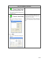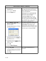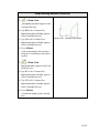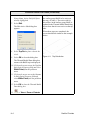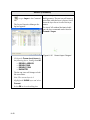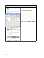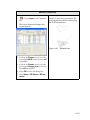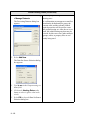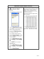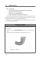
10 Tutorials
This chapter presents information and sample problems to explore some of Thermal
Desktop’s features. Before beginning the tutorials, AutoCAD 2000/2000i/2002/2004, Thermal Desktop, and SINDA must be installed. Refer to the AutoCAD and Thermal Desktop
installation instructions to complete these installations if the software is not already installed.
Tutorial files may be found in the \Tutorials subdirectory which is located in the Thermal
Desktop installation directory (usually C:\Program Files\Cullimore And Ring\Thermal Desktop). The Tutorials subdirectory includes additional subdirectories, one for each of the tutorials covered in the subsequent sections of this chapter. As tutorials are successfully completed, a \completed directory is created with the results of that tutorial.
It is recommended that the Tutorials directory be copied to the user’s own working area
before beginning the tutorials. This ensures a copy of the original tutorial files will be
available for use by other users at a later time.
The tutorials attempt to introduce a variety of concepts. Most often there is more than
one way to accomplish the “task” of a tutorial. Different techniques are shown in an attempt
to expose the user to the variety of features present in Thermal Desktop. In particular, there
are many ways of selecting objects, and both noun-verb and verb-noun order is supported
for most commands. Identical tasks may be performed differently to illustrate a particular
feature.
It is also strongly suggested that each new user take the time to work through each of
the tutorials (in this chapter as well as the other tutorial chapters (see “RadCad Tutorials”
on page 11-1 and see “FloCad Tutorials” on page 12-1). Although completing the tutorials
requires time, doing so will provide the user with enough knowledge and skills to allow the
user to quickly become effective and efficient while working in Thermal Desktop.
There are seven tutorials in this chapter, as follows:
• Section 10.1: Getting Started on page 10-5
• Section 10.2: Setting Up a Template Drawing on page 10-33
• Section 10.3: Circuit Board Conduction Example on page 10-37
• Section 10.4: Beer Can Example on page 10-55
• Section 10.5: Combined Radiation/Conduction Using Finite Elements on page
10-94
• Section 10.6: Mapping Temperatures From a Course Thermal Model to a
Detailed NASTRAN Model on page 10-120
• Section 10.7: Model Browser Example on page 10-139
• Section 10.8: Simple Meshing Methods on page 10-151
• Section 10.9: Dynamic SINDA Example on page 10-161
• Section 10.10: Parameterizing for a Common Input on page 10-185
Tutorials
10-1
Functionality in the tutorials reflects the most recent version of Thermal Desktop. Every
effort has been made to present the user with the exact system prompts, messages and
commands, and dialog boxes the user will see when using Thermal Desktop. Please note
that occasionally minor changes may be made between application releases and, as such,
small changes to wording in such items may be experienced. The “how to” functionality
will not change.
Typographical conventions used in the examples are as follows:
Typographical Conventions
•
Prompts, instructions and other lines of text directed to the user that appear in the
Command Line area, dialog boxes and such are shown in Arial type font. For example:
Specify base point or displacement:
•
Actions requiring input by the user will be numbered and shown in italic font:
1. Pick a point or enter coordinates.
•
User response, meaning text which is to be typed by the user exactly as shown, is
written in bold Arial type font. The user many be prompted to input, or type,
information into the Command Line area, into a dialog box or some other text box.
For example:
Command: 3dface
or combined with a numbered action requiring user input:
2. Type 9x in the Command line.
10-2
Tutorials
Typographical Conventions (Continued)
•
Menu functions are shown in bold Arial type font. Selecting commands from a
cascading pulldown menu is shown using Arial type font, starting with the top
level choice, and with a right facing angle bracket ( > ) used to show selections on
the cascading menus:
Thermal > Surfaces/Solids > Disk
Thermal > Surfaces/Solids > Disk represents the user clicking on, or selecting,
the pulldown menu selections, beginning with Thermal, located on the menu bar:
Figure 10-1
Tutorials
Pulldown Menu Example
10-3
Typographical Conventions (Continued)
•
Pressing the Enter key is implied after entering text in response to a command
prompt.
The symbol <Enter> represents pressing the Enter key when no text is to be
entered but an Enter key entry is required.
Anytime the user is required to press a function or other keyboard key, the key will
be shown in bold Arial type font and enclosed in angle brackets. For example, if
the user is to press function key F2, the key is shown as follows:
<F2>
Many menu functions have the option of using shortcut keyboard commands comprised of holding down a key such as the Control (Ctrl) key and then holding down
an additional key. If a menu has such an option, the shortcut keyboard command
may be included in the exercise options. The keys to be pressed will be shown in
bold Arial type font and enclosed in angle brackets. For example, if the user wants
to copy text the Copy function can be performed by highlighting the text and clicking on Edit on the menu bar followed by clicking on Copy. The Copy function has a
shortcut keyboard command Control key and the C key, or:
<Ctrl><C>
•
When an icon exists to perform the same function as a pulldown menu command, it
will be displayed as:
or Thermal > Surfaces/Solids > Disk.
The user can either double click on the icon on the tool bar or select the displayed
sequence of menu picks from the pulldown menu.
In many instances, the user has the option of selecting an icon, making a pulldown
menu selection or typing in a command in the Command Line area. In these
instances, the user may use any of the options.
If the user is required to click on an icon and there is no corresponding pulldown
menu choice (for example launching Thermal Desktop/AutoCAD), the icon and the
name of the icon will be displayed:
Thermal AutoCAD icon.
•
10-4
If a command is mistyped, press the Escape key, or <Esc>, to cancel the command
in progress. Edit > Undo may also be used to undo an action.
Tutorials
10.1
Getting Started
The Getting Started section of the tutorial is broken into several different sections. These
sections are:
•
User Interface
•
Graphical Objects
•
Grip Points
•
Selection
•
Pan/Zoom/Rotate
•
Shading/Wireframe
•
Layers
•
Colors
The section offers information and, in some cases, instructs the user to perform an action
as a means to familiarize the user with Thermal Desktop functions.
Tutorials
10-5
10.1.1
User Interface
This section provides an overview of the User Interface detailing icons, Thermal pulldown menu commands, and various components of the main AutoCad window.
User Interface
At this point, you should start up AutoCAD. The way to start AutoCAD is a function of the flavor of AutoCAD that you have installed.
The first thing to check is if you have a Thermal Desktop Icon on your Desktop. If
you have that, go ahead and double click on that icon. That will startup our OEM
version of AutoCAD, either based on AutoCAD 2002 or AutoCAD 2005.
If you don’t see a Thermal Desktop icon on your Desktop, go to Start>Programs>
and look for AutoDesk or AutoCAD 2000/2000i/2002. If you see AutoCAD 2002/
2000i/2002, then follow that to the AutoCAD executable (i.e.Start>Programs>AutoCAD 2002>AutoCAD 2002). If you see AutoDesk, follow that to the
version of AutoCAD installed, and then follow that to the executable (i.e. Start>Programs>AutoDesk>Mechanical Desktop 2005>AutoCAD 2005.
If you still haven’t seen how to start the program, try Start>Programs>Cullimore
And Ring>Thermal Desktop>Thermal Desktop.
Important: Please note that if you have Mechanical Desktop
installed, the Thermal Desktop will run fine, but the AutoCAD
interface for Mechanical Desktop is very different than regular
AutoCAD, and tutorials are written for regular AutoCAD. In
this case, you should run regular AutoCAD to do the tutorials
and not Mechanical Desktop.
Important: If it is not possible to complete the Getting Started
drawing (drawing1.dwg) in the same setting, exit Thermal
Desktop (File > Exit) and respond No when prompted to save
the drawing. To save the drawing, perform a Save As and
change to a directory other than the initial system installation
directory.
10-6
Tutorials
User Interface (Continued)
The Thermal Desktop/AutoCAD window appears with the Startup dialog
box displayed. If you do not see this
window, that is not a problem, just go
ahead and go to the next step.
The English/Metric choice in the Startup
dialog box does not set units for Thermal
Desktop. This setting is used for setting
up a drawing grid and for setting up plotting to a printer. Either choice may safely
be used.
The Units of the Thermal Desktop model
are set with the Thermal > Preferences, Units Tab command. The
default units are metric with the length
being meters.
3. Select Start From Scratch in the
Startup dialog box (second icon from
the left) if not already selected.
Note: If a startup menu does not appear, then you are in the default of
start from scratch. Just go to the
next step in the tutorials.
4. Select OK to close the dialog box.
Tutorials
10-7
User Interface (Continued)
A Thermal Desktop/AutoCAD dialog
box appears (may appear) stating the
default directory for the new drawing,
named Drawing1.dwg, is the
AutoCAD installation directory.
5. Select OK to close the dialog box.
10-8
It is recommended that drawing files are
not saved to the default directory but to
another directory created by the user
where the drawings can be easily
accessed.
The starting directory is where all the
files Thermal Desktop generates will
reside. When this is the installation directory, sometimes users can’t find their
files, or don’t even have write permissions to the directory. Double-clicking on
the .dwg file to start a model is much preferred than Starting AutoCad and performing a Save As command.
Later in the tutorial, a drawing template
will be created. The template will then be
copied for each new model, keeping the
template in its original form. It is recommended this process be followed, copying
the template to a directory or folder that is
associated with the work being performed, renaming the template to a logical name, and then double clicking on the
newly renamed .dwg file to open Thermal
Desktop.
Tutorials
User Interface (Continued)
The Thermal Desktop window may
display with the Property window displayed to the side of the screen.
Figure 10-2
Properties Window
6. Close the Properties window.
The Properties window will be discussed later in the tutorials.
Figure 10-3
Tutorials
Screen without Properties Window
10-9
User Interface (Continued)
1. Select Thermal > About Thermal
Desktop...
Note: A dialog box may appear instructing the user to set a profile.
The profile controls how the user interface looks.
This dialog box will not appear for
users that have Thermal Desktop with
CAD built-in.
• Click Yes, if the Profile dialog
box appears.
The About Thermal Desktop/
RadCAD/FloCAD dialog box appears
displaying version, license, author and
C&R Technologies information.
If the Thermal pulldown does not exist,
then the menus have not been installed
properly. This can be fixed by executing
Start > Programs > Thermal Desktop >
User Menu Setup.
For those users the Thermal Desktop version without CAD, a Profile dialog box
may appear. A profile controls how the
menus come up on the screen. Advanced
users may want to set up different profiles
for different AutoCAD applications. This
dialog box will not come up if Thermal
Desktop is already the current profile.
Finally, the About Thermal Desktop
screen displays which version of the software is installed, and what the user has a
license for.
2. Select OK on the About Thermal
Desktop/RadCAD/FloCAD dialog
box.
10-10
Tutorials
User Interface (Continued)
Figure 10-4 shows the opening default screen with the exception that the drawing
background is white instead of black. The change in color is to facilitate the reproduction of this manual.
Much of the screen utilizes standard Windows elements such as title bars, a main menu
bar and various toolbars.
The Thermal menu contains all of the commands specific to Thermal Desktop. The
other menu options located on the menu bar contain commands created by AutoCAD,
many of which are standard Windows commands. The AutoCAD commands (MOVE,
COPY, ARRAY, etc.) work on the Thermal Desktop objects.
As with other Windows based applications, most of the commonly used menu commands have associated toolbars displaying icons corresponding to menu commands.
Toolbars provide quick access for the user to perform a command. There is no difference between using a pulldown menu versus using a toolbar icon to perform a command.
The toolbars are arranged in three primary groups.
•
Toolbars located on the left of the screen are used for creating entities such as surfaces, nodes, lumps, and conductors.
•
The toolbars located on the right of the screen are used to edit the entities, as well as
change what is viewed such as active sides and post processing.
•
The toolbars located at the top of the screen are used to open and save files, manipulate layers, and also to rotate/pan/zoom a view.
To learn what each icon on the toolbar represents, position the cursor over an icon and
then stop moving the mouse. When the cursor pauses over an icon a short text description called a tool tip is displayed. The tool tip shown in Figure 10-4 at the top left,
shows the command to create a Thermal Desktop rectangle.
At the lower left of the graphics area, the UCS (User Coordinate System) icon is displayed. All points input and displayed are in this coordinate system. In this display, a
“W” is displayed on the axis. This “W” stands for world, meaning the view uses the
world coordinate system. The UCS icon shown in Figure 10-4, is the 2D format. A 3D
UCS icon is available under View > Display > UCS Icon > Properties.
Also located at the lower left of the screen, the current location (X, Y or X, Y, Z) of the
cursor in the drawing area is displayed. As the cursor is moved in the drawing area, the
coordinates change as the cursor moves. This update can be very handy when selecting
points on the screen.
Tutorials
10-11
User Interface (Continued)
At the bottom of Figure 10-4 resides the Command Line area. The Command Line
area is where the user will be prompted to type in a command or value(s) and will see
various messages. While the user can only see a few lines of text in that area, the entire
text area can be displayed by selecting the <F2> function key.
1. Press <F2> to open the Thermal Desktop Text Window.
Use this window to view commands and actions performed in the current session.
2. Press <F2> again to close the window.
Menu Bar
Layer Pulldown Menu Color Pulldown Menu
Thermal Pulldown Menu
Icons to Open, Save, Layers, and pan/rotate/zoom
Tool tip
Drawing/Graphics Area
Icons to edit
and manipulate
what is displayed
Icons to create
UCS Icon
Command Line area
Current Point
(Cursor Coordinates)
Precision Drawing/
Lineweight/Model Buttons
Status Bar
Figure 10-4 Default Thermal Desktop Window
10-12
Tutorials
10.1.2
Graphical Objects
This section introduces the user to some general Thermal Desktop functionality.
Graphical Objects
1. If Thermal Desktop/AutoCAD is not
currently running, launch Thermal
Desktop.
2.
or Thermal > Surfaces/Solids > Rectangle.
Command: _RcRectangle
Origin point <0.0.0> appears in the
Create an arbitrary rectangle by following
the steps noted to the left. The actual
coordinates are not important.
The picture should look similar to Figure
10-5. The boundaries of the rectangle are
shown by the solid lines, and the circle in
the middle represents the node associated
with the rectangle.
Command Line area.
3. Click on a point in the lower left of
the graphics area with the cursor.
Point for +X axis and X-size <@1,0,0>
appears in the Command Line area.
4. Click on a second point in the
graphics area that is to the right of the
first point.
Point to set XY plane and Y-size
<@0,1,0> appears in the Command
Line area.
5. Click on a third point in the graphics
area that is above the second point.
Tutorials
10-13
Graphical Objects (Continued)
The Thermal Model Data dialog box
appears.
When viewing the rectangle, solid lines
are visible around the outside of the rectangle. In the center of the rectangle is a
node. Dashed lines from the sides of the
rectangles to the nodes may or may not be
visible. These dashed lines represent the
node locations.
6. Select OK to close the dialog box
without making any changes.
The rectangle is created.
10-14
Tutorials
Graphical Objects (Continued)
Dashed Lines
Solid Lines
Node
Rectangle
Figure 10-5 Getting Started - Building a Rectangle
The rectangle in Figure 10-5 has arrows pointing to dashed lines and solid lines. The
solid lines represent the node boundaries, and the dashed lines represent the lines that
the node resides on. The user can control how many dots are used to represent the
dashed lines with the LTSCALE command.
When the geometry gets very complicated, sometimes it is easier to select a surface by
clicking on the dots instead of a boundary that might be shared with another object.
7. Type LTSCALE in the Command
Line.
Enter new linetype scale factor
<1.0000> appears.
8. Type .1
The number displayed in < > after issuing
the command LTSCALE is the current setting for LTSCALE. Entering a smaller
number will display more dots in the
dashed lines, while a larger number will
display less dots.
Additional dashed lines appear.
Tutorials
10-15
10.1.3
Grip Points
This section demonstrates the use of grip points to edit a surface. Grip points provide
for an immediate, interactive editing of objects without entering any specific commands on
the command line. Grip editing is a quick and easy way to modify an object.
Grip Points
When an object is selected with the mouse, the object’s solid lines change into dashed
lines and grip points (small squares) become visible. The grip points’ color is often preset
to blue, but the user can control grip point color and size by selecting Tools > Options...
and then clicking on the Selections tab in the Options window, as shown below.
Figure 10-6
Options Selection Tab
Grip points provide an easy form of editing an object.
10-16
Tutorials
Grip Points (Continued)
1. If not already opened, launch Thermal Desktop and create a rectangle as
shown in the previous tutorial (See Section 10.1.3.
2. Select the rectangle by positioning the cursor on one of the solid lines making up
the rectangle and clicking the mouse.
The solid lines change to dashed lines and grip points appear at various points on
the rectangle.
3. Position the cursor over one of the grip points.
A tool tip associated with the grip point appears.
As shown in Figure 10-5, the tool tip at the end of the X axis of the rectangle
(Stretch X Length) instructs the user that the grip point associated with that tool tip
can be used to modify the X length the rectangle.
4. Click on the grip point referenced above.
The grip point changes color and the tool tip Endpoint is displayed.
5. Move the cursor to a new point and click the mouse button.
6. View the change to the rectangle.
7. Select <Ctrl><Z> key to cancel the operation.
The rectangle returns to its previous dimensions and is deselected (no longer highlighted).
Note: The <Esc> key can also be used to deselect an object.
8. Position the cursor on the other grip points on the rectangle to view the tool tip
messages.
Tutorials
10-17
10.1.4
Selecting Objects
The selection of objects is probably the most difficult new things to learn when working
with a CAD program and this section introduces the user to some basic selection concepts.
Selecting Objects
There are two types of selection, pre-selection and post selection.
•
Pre-selection means one or more objects are selected and then a command such as
Thermal > Edit or Modify > Copy is issued.
•
Post selection means a command is issued and then one or more objects are
selected. The cursor changes shape (box) and waits for the user to select the
object(s) to be affected and click the right mouse button. Post selection only works
if nothing is selected when the command is issued.
The easiest way to make sure nothing is selected before you issue a command is to
press the <Esc> key. Pressing <Esc> resets the selection set to empty. In AutoCAD
2000, the <Esc> must be selected twice.
The cursor appears as crosshairs with a square box, called a pick box, in the middle
of the cursor (Figure 10-7). When selecting an object, position the cursor over the object
to be selected. The item positioned within the pick box is the object that will be selected
when the mouse is clicked.
In the left-most graphic in Figure 10-7, the pick box includes the solid line of a
rectangle. When the cursor is paused over an object, the tool tip associated with the object
displays what is being selected. The tool tip shows the type of object, followed by an
object identifier (format ::OBJECTID), which is unique for each object.
Note: If the tool tip doesn’t display, select Tools > Options,
User Preferences and make sure Display hyperlink tool tip
is selected (check mark in the box).
10-18
Tutorials
Selecting Objects (Continued)
Still working with Figure 10-7, the cursor is positioned over the node which is located
in the center of the rectangle. If the cursor is positioned over the node as shown in the
center graphic, the tool tip still shows the rectangle as the object. This is because there
are two items in the pick box—the dashed lines of the rectangle, and the solid circles
from the node. The user has limited control over what will be selected in this instance;
however, there are two methods to assist in choosing the node:
•
Method 1: The easiest method is to move the cursor so that only the node is in the
pick box, as shown in the example on the farthest right of Figure 10-7.
•
Method 2: The second method is to select the rectangle, then select Tools >Display Order > Send to Back. This will make the node be the first item selected
when the rectangle and the node are both in the pick box.
A third option is to hold down the <Ctrl> key, which will cycle through the items
available in the pick box. This last option can be tedious and difficult to learn, but may
be worth investigating as an additional option.
Pick Box
Figure 10-7
Getting Started - Selection
The size of the pick box can be changed by typing PICKBOX in the Command line
and changing the input value. The default value of 3 is often too small to be useful; many
users prefer a value of 5.
Tutorials
10-19
Selecting Objects (Continued)
Selecting objects one at a time is a common occurrence but there many times when
a user may want to select multiple objects without having to go through the process of
selecting and performing an operation on each object individually. Multiple objects can
be selected by first drawing a box around a group of objects to select them and then
performing an operation. As simple as this seems, there are different methods to encircle
some objects for selection, and these different methods will result in different selection
sets.
Using Figure 10-8 as an example, consider the situation of an Ellipse, Disk, and a
Line. Drawing a box around all three of the items will result in all three being selected.
The selection set will be different when the drawing box crosses the lines of some of the
items as shown with the solid black line. If the user draws the box by picking in the upper
left corner (#1) and then dragging the cursor to the lower right (#2), only the items completely enclosed in the box will be selected. In this case, only the disk is selected.
If the user reverses the order of drawing the box by picking in the lower right corner
(#2) first and then dragging the cursor to #1, the items enclosed and crossing the box will
be selected. In the case shown in Figure 10-8, all three of the of the items will be selected.
The drawing box method of selecting multiple objects will be used in a future tutorial,
the “Beer Can Example” on page 10-55.
1
2
Figure 10-8
10.1.5
Getting Started - Selection Boxes
Pan, Zoom, Rotate, and Views
This tutorial demonstrates several methods of changing the view on the screen. The view
can be zoomed in for a closer view of an object or zoomed out for a higher-level view of
an object or a drawing. The view can be panned—moved to the right, left, up or down—
which will change the view on the screen without zooming in or out. Changing the view of
a drawing or a specific object can assist the user when creating detail
Graphical Objects
1. If not already opened, launch Thermal Desktop and create one or more rectangles
as shown in the previous tutorial (See Section 10.1.3.
10-20
Tutorials
Graphical Objects (Continued)
or View > Zoom > Realtime.
2.
The cursor changes into a small magnifying glass with plus and minus
signs.
3. Move the mouse up and down on the
screen.
The view zooms in (closer, more
detail) as the mouse is moved upward;
the view zooms out (higher level, less
detail) as the mouse is moved downward.
Use this function to enlarge the view of
the objects on the screen (zoom in, more
magnification) or decrease the view of the
objects (zoom out, less magnification) as
the mouse is moved.
Note that when Zoom Realtime is initiated, the message Press ESC or ENTER
to exit, or right-click to display shortcut
menu appears in the Command Line area.
Remember to look to the Command Line
for additional information.
4. When finished, right mouse click
and select Exit from the drop down
menu
or View > Pan > Realtime.
1.
The cursor changes into a small hand.
2. Move the mouse up and down on the
screen.
The view zooms in (closer, more
detail, more magnification) as the
mouse is moved upward; the view
zooms out (higher level, less detail,
less magnification) as the mouse is
moved downward.
Use this function to change view on the
screen by shifting the view up, down, left
or right as the mouse is moved. The magnification level does not change (no zoom
in or zoom out occurs).
Note that when Pan Realtime is initiated,
the message Press ESC or ENTER to
exit, or right-click to display shortcut
menu appears in the Command Line area.
Remember to look to the Command Line
for additional information.
3. Leave the view on the screen so that
some of the object(s) are off to the side
or not visible.
4. When finished, right mouse click
and select Exit from the drop down
menu
Tutorials
10-21
Graphical Objects (Continued)
or View > Zoom > Extents.
1.
2. All of the objects in the drawing are
moved back into view.
or View > Zoom > Window.
1.
Specify corner of window: appears in
the Command line.
2. Pick on a point that represents the first
corner of a rectangle that will enclose
the object/area to be viewed.
Specify corner of window: Specify
opposite corner: appears in the Com-
mand line.
3. Pick at point diagonally opposite the
first point. A box is drawn around the
area between the two points as the
cursor moves.
The view zooms in around the area
enclosed by the rectangular area
defined by the two points.
4. Click the right mouse button and
select Zoom > Extents to return the
drawing area to its full extents.
Adjusts the view on the screen by
zooming out until all objects in the drawing
are visible. Use this function if a desired
object or area is no longer within the drawing area because of panning or zooming.
This function will quickly return to the
complete drawing area view.
Use this function to quickly zoom into a
specific object or area in the drawing
area. This command has the user define a
rectangle that encloses the portion of the
drawing area to be viewed by clicking on
two points. The first point sets a first
“corner” of the rectangle; the second
point determines the opposite, diagonal
corner of the area to be viewed.
Note that when zooming and panning, the
right mouse menu can be used to switch
between the various zooming and panning options.
When Zoom > Window is initiated
from the right mouse menu, the cursor
changes into a pointer with a filled-in box
attached to it. Move the cursor to a point
that represents the first corner of the area
and then hold down the left mouse button
and drag the mouse to a point opposite the
first point. Release the mouse button.
5. When finished, right mouse click
and select Exit from the drop down
menu
or View > Zoom > Previous.
1.
Use this function to quickly return to the
last zoom/panned view.
The view in the drawing area returns
to the last view in the zoom/pan
sequence.
2. When finished, right mouse click
and select Exit from the drop down
menu.
10-22
Tutorials
Graphical Objects (Continued)
2. Position the cursor within the arcball.
Use this function to 3D view a drawing.
When activated, a circle, called an arcball,
appears around the selected object. As the
user selects points and drags the mouse, the
view of the selected object changes so the
user sees the object from whatever angles
the user desires (vertically and horizontally).
The cursor changes shape (two arrows
circling a sphere).
A special right mouse menu offers additional 3D view options.
1.
or View > 3D Orbit.
An arcball appears on the screen. The
arcball is a large circle, or sphere.
There are four smaller circles at the
quandrant points on the arcball.
3. Hold down the left mouse button and
drag the cursor within the arcball.
The rectangle (or all objects if more
than one object is in the drawing area)
rotates in all directions. Watch the
USC icon as the cursor moves.
4. Release the mouse button. Position the
cursor outside of the arcball.
The cursor changes shape (an arrow
circling a sphere).
5. Hold down the left mouse button and
drag the cursor outside of the arcball.
The object rotates around an axis a the
center of the arcball.
6. Release the mouse button. Position the
cursor on one of the quadrant circles.
The cursor changes shape (an arrow
elliptically circling a sphere). This
function changes the vertical and/or
horizontal rotations of the object(s).
7. Hold down the left mouse button and
drag the cursor away from the quadrant circle.
Tutorials
10-23
Graphical Objects (Continued)
The object(s) rotate around a horizontal axis (if the 3:00 or 9:00 quadrant
circles were selected) or around a vertical axis (if the 12:00 or 6:00 quadrant
circles were selected).
8. Release the mouse button and right
click to display the right mouse menu.
The 3D Orbit right mouse menu offers
zoom and pan commands as well as
various shading and projection commands. Clicking on More displays the
pulldown menu shown above
9. Press <Esc> three times to close right
mouse menus and end the 3d Orbit
command.
10-24
Tutorials
Graphical Objects (Continued)
1. Click on View > 3D Views.
The 3D Views pulldown menu appears.
Many predefined orientations are shown
under View > 3D views.
The user can also create and store views
of particular areas of a drawing with the
View > Named Views function. View
> Named Views allows a user to
quickly return to a previously designated
area of a drawing.
2. Select View > 3D Views > SW Isometric.
The view of the rectangle (or other
objects in the drawing area) changes to
that of the SW Isometric view.
3. Select View > 3D Views > Top.
The view of the rectangle (or other
objects in the drawing area) changes to
a top-down view of the rectangle.
4. Repeat additional view options as
desired.
10.1.6
Shading/Wireframe Views
The Shade and Wireframe View commands offer the user different ways to view models.
Tutorials
10-25
Shading & Wireframe Views
The Shade and Wireframe commands are found under the View > Shade pulldown
menu.
The first three items in the pull down are 2D Wireframe, 3D Wireframe, and Hidden.
The differences between the three can be subtle, but each has it’s uses. Figure 10-9
illustrates the differences in the three views.
•
2D Wireframe: Shows dashed lines to locate the nodes.
•
3D Wireframe: Does not show the dashed lines; surface boundaries are more
defined.
•
Hidden: This view is similar to 3D Wireframe but the lines behind surfaces are
removed, making the image on the right easier to see.
Figure 10-9
10-26
Getting Started - 2D - 3D wireframe and Hidden views
Tutorials
Shading & Wireframe Views (Continued)
There are four options for shaded modes—Flat Shaded, Gourand Shaded (Smooth
Shaded), Flat Shaded, Edges On and Gourand Shaded, Edges On. Of the four modes,
the Gouraud Shaded option is the best looking and the most often used.
Toolbar icons exist for the 2D/3D Wireframe, Hidden, and Gouraud shaded commands.
These icons are in the top toolbar as shown in Figure 10-4.
Below is an example of an object viewed using the seven View > Shade commands.
Figure 10-10
10.1.7
Shade Examples
Layers
Everything in a drawing is associated with a layer. Layers are separate drawing areas,
one on top of the other, and are used to organize and to manipulate what is currently being
viewed in a model including the color, linetype and lineweight of an object. Layers are a
good way to group and display related objects in a drawing or model.
When a new object is created, it is placed on the current layer. Layer properties such as
name and color are managed in the Layer Properties Manager dialog box and by using
additional Layer controls. Figure 10-11, shown below, shows the Layer Properties Manager. The Layer pulldown menu is included on Figure 10-4 and discussed later in this
section.
Note: Changing object layers will be discussed later in the tutorial.
Tutorials
10-27
Every model has a layer numbered 0. The 0 layer is system generated and cannot be
deleted or renamed. Another layer, the ASHADE, is internally used by AutoCad to control
the lighting settings of the objects. The ASHADE layer is locked. Locking a layer means
the entities cannot be changed.
Important: C&R Technologies highly recommends that the
user does NOT lock layers, as odd results can occur. Please also
note that AutoCAD 2000 version models will not have an
ASHADE layer unless the user invokes Render commands.
The next section creates a new layer and familiarizes the user with the Layer Properties
Manager.
Layers
1. If not already opened, launch Thermal Desktop and create one or more rectangles
as shown in the previous tutorial (See Section 10.1.3 if no objects are displayed.
Create a new layer to be called layer1.
2.
or Format > Layer.
or type layer in the Command Line.
Current Layer
Figure 10-11
10-28
Getting Started - Layer Manager
Tutorials
Layers (Continued)
The Layer Properties Manager
appears. The two default system-generated layers are listed.
Note: A layer (other than layers 0
and ASHADE) may be renamed by
clicking the layer name twice to select it and typing in the new name.
3. Select New.
A new line is added for Layer1.
4. Select the light bulb icon in the On
column of the new Layer1.
The icon changes and “turns off”
(darkens).
5. Select the color icon for layer 0 (currently White).
The Select Color dialog box appears.
6. Select Red from the standard colors
selections to change 0’s value to red
(top left).
7. Select OK to close the Select Color
dialog box.
The Color value for 0 should display
the color red in the Layer Properties
Manager.
Next to the layer names are two columns
with icons underneath the column headings.
•
On
•
Freeze in all VP
Note: VP is an abbreviation for
viewport.
These icons control whether or not
objects residing on a layer are displayed
or not. If either the On or Freeze in all VP
icons are off (blue), then the objects will
not be seen graphically. If the Freeze in
all VP icon is blue, then the object won’t
be included when ALL is entered at the
select prompt. While this is very subtle, it
can explain why the ZOOM ALL command may not fit the model properly in
the window.
When the Layer Properties Manager is
closed, note the objects within the graphical screen have changed to red.
8. Select OK to close the Layer Properties Manager.
Tutorials
10-29
Layers (Continued)
9.
or Tools > Properties or type
properties in the Command area or
press <Ctrl><1>.
Every graphical object has properties
associated with them, some of which can
be changed by the user as needed. Double-clicking on an object will bring up the
Properties window. This form is modeless and can stay up while working in
AutoCAD.
The Properties dialog box appears.
Note that layer 0 is the current layer.
10. Select a of rectangle on the screen.
The Properties dialog box changes to
show a list of property values.
10-30
Tutorials
Layers (Continued)
The Layer pulldown menu, shown to the
left and in Figure 10-4, can be used to
manipulate some layer properties without
having to open the Layer Properties Manager. These properties are:
11. Click on the Layer pulldown menu
arrow and select Layer1.
A Thermal Desktop/AutoCAD dialog
box appears stating 1 object changed
to a frozen or off layer and removed
from the selection set.
Remember that Layer1 was turned off
in the Layer Properties Manager.
12. Click OK to close the Thermal Desktop/AutoCAD dialog box.
The rectangle is no longer visible on
the screen.
13. Click on the Layer pulldown menu
arrow and select the On icon (light
bulb that is currently blue—off) for
Layer1.
The rectangle previously selected
reappears on the screen, in white,
Layer1’s default color.
14. Click on the X in the upper right corner of the Properties dialog box to
close it.
Tutorials
•
Turn a layer On of Off
•
Freeze or thaw in ALL viewports
•
Freeze of thaw in current viewports
•
Lock or Unlock a layer
•
Color of layer
Once a rectangle is selected, the Color
box says “ByLayer”. Color of an entity
can be changed from the By Layer setting.
When changing to a different layer, if no
objects are selected and the layer is
changed, then the selected layer becomes
the new “current” layer and all new
objects will be created on that layer.
If one or more objects are selected when
the layer is changed using the Layer pulldown menu then the selected objects will
be moved to the newly selected layer.
When an object’s layer is changed to one
that is not visible, a warning dialog box
appears. Also note that when the layer of
an object is changed, the node associated
with the object is also changed to the
same layer.
10-31
10.1.8
Colors
Colors
Just as each object has a layer associated with it, an object has a color associated with
it. The default color for objects is set to Color By Layer, which means the color of an
object is the same as the color defined for the layer, which is set in the Layer Properties
Manager, from the Layer pulldown menu or by clicking on Color in the Properties dialog
box and selecting a color from the pulldown menu as noted above in Section 10.1.7.
If changing an object’s color using the Color pulldown menu, shown above and in
Figure 10-4, while no objects are selected, then the color selected will become the default
color for newly created objects.
If an object’s color is changed using the Color pulldown menu when one or more
objects are selected, the selected items will be assigned the newly selected color.
All colors that are assigned to objects will be overridden by Thermal Desktop when
post processing of data or Display Active Sides is performed.
15. Select File > Exit.
A Thermal Desktop/AutoCAD dialog
box appears asking to save the drawing changes.
Exit Thermal Desktop and respond no
when prompted to save the drawing.
16. Select No.
10-32
Tutorials
10.2
Setting Up a Template Drawing
A template is something that can be used as a pattern for future projects. In Thermal
Desktop, a template drawing file can be created and used as a foundation for creating new
Thermal Desktop drawings. When creating a template it is important to consider how the
template will be used, if the template will be used by only one user or by more than one,
what preferences should be associated with the template and other such considerations.
In this tutorial, a template drawing file (file extension .dwg) will be created. The template
will be used in some of the upcoming tutorials and may be used as a permanent template
for use in future thermal analysis tasks. Creating and then using a template drawing starts
a new analysis with an environment set to pre-determined preferences, helping to keep
drawings consistent and easy to use.
Before beginning a new thermal analysis task, copy the template to a directory chosen
to store the work for that particular task or project. Once a copy is made, rename the copied
template drawing to a meaningful name related to the thermal task or project. Then start
Thermal Desktop by double-clicking on the renamed drawing file. Thermal Desktop will
start with the preferences saved in the template, and the current working directory will be
set to the directory which contains the drawing file. All database files created by Thermal
Desktop for view factors, radiation conductors, and orbital heating rates will be placed in
this working directory.
Important: If Thermal Desktop is not launched using the drawing
file for the task and instead is started from the AutoCAD Icon,
the current working directory will be the Thermal Desktop installation directory. This is not recommended, since multiple
thermal analysis tasks may overwrite each other’s database files.
Data stored in the AutoCAD installation directory may also be
lost when installing future upgrades.
The following exercise creates a template file with preferences set to be convenient for
working with Thermal Desktop. The user is encouraged to experiment with the available
options as a means to discover which settings are compatible to each individual’s work style.
Setting Up a Template Thermal Desktop Drawing File
1.
or Thermal Desktop/AutoCAD icon or, for getting started the first
time, select Start > Programs > Thermal Desktop > Thermal Desktop.
Tutorials
10-33
Setting Up a Template Thermal Desktop Drawing File
The Thermal Desktop/AutoCAD window appears with the Startup dialog
box displayed.
2. Select Start From Scratch in the
Startup dialog box (second icon from
the left) if not already selected.
3. Select OK to close the dialog box.
The drawing area title bar changes to
the default drawing name
Drawing1.dwg.
4. Select View > 3D Views > SW Isometric.
Note the UCS icon changes to reflect
the view.
10-34
This section of the tutorial creates a new
drawing to be used as a template that will
be copied and renamed as future drawings
are created.
English (Feet and Inches) and Metric are
default settings, English pre-selected. The
English/Metric settings in this dialog box
do not set the units for Thermal Desktop.
This setting is used for setting up a drawing grid and for setting up plotting to a
printer. Either choice may be safely used.
Note: Units of the Thermal Desktop
are set by selecting Thermal > Preferences, and then selecting the
Units Tab. The default units are
metric with the length being meters.
3D Views will be discussed in further
detail later in the tutorial. Selecting View
> 3D Views > SW Isometric here sets
an isometric view parameter for the new
template.
Tutorials
Setting Up a Template Thermal Desktop Drawing File
5. Select View > Display > UCS
Icon> Origin.
This step locates the User Coordinate
System (UCS) display icon at the origin
of the model, rather than in the lower left
corner of the screen.
If the UCS origin is not in the display
area, then the UCS will be displayed in
the lower left corner.
6. Confirm a check mark is displayed next to Origin. If a check
mark is not visible, click the left mouse
on Origin to select the option.
Note: Depending upon the experience and preferences of the user, before saving
the template the toolbars on the main window may be rearranged. The default
arrangement of toolbars reduces the horizontal size of the viewport. The toolbars
can be moved to the sides of the viewport to produce a viewport with a more
square aspect ratio. Put the cursor in the border of a toolbar (not on an icon) and
drag by holding the left mouse button down to the new desired location. As a
toolbar is moved close to the sides of the screen, the toolbar will automatically
dock to that side.
The View >Toolbars menu choice may also be used to turn specific toolbars on
and off and to customize the icons in each toolbar. See the AutoCAD help for more
details on customizing toolbars. It is helpful to remove infrequently used icons from
some toolbars so that more toolbars may be displayed without taking up excessive
screen space.
Tutorials
10-35
Setting Up a Template Thermal Desktop Drawing File
7. Select File > Save As.
The Save As dialog box appears.
Be sure to save the files in your copy of
the tutorials directory.
8. Change the name of Drawing1.dwg to
thermal in the \Tutorials\template
directory.
9. Select Save.
The drawing area title bar is updated
with the new name of the drawing,
thermal.
10. Select File > Exit.
Thermal Desktop is closed.
As experience is gained with Thermal Desktop and some of the advanced options, create
a new template file with different parameters such as Units and other property settings as
desired.
Important: Remember to create a copy and rename the template
before beginning design work to insure the template remains
in its original state. If copying the template at the directory/file
level by dragging the template file icon to the working directory,
be sure to hold the <Ctrl> key down when dragging the template
drawing file so that the template is copied, rather than moved.
10-36
Tutorials
10.3
Circuit Board Conduction Example
What you should learn:
• Overview of how Thermal Desktop works
• How to create material properties
• How to apply edge contact resistance
• How to apply area contact resistance
In this exercise, a circuit board will be mounted to an aluminum face. The circuit board
will have a chip placed on it.
Circuit Board Example
1. Copy the template thermal.dwg file created in the first tutorial to the \Tutorials\board directory.
Note: Be sure to hold the <Ctrl> key down if dragging the template file icon to
the new directory so that the file is copied, rather than moved.
2. Rename the copied template file to board.
3. Start Thermal Desktop by double clicking on the board drawing file icon in
the board directory.
Tutorials
10-37
Circuit Board Example (Continued)
1. Select Thermal > Thermophysical
Properties > Edit Property Data.
The Edit Thermophysical Properties
dialog box appears.
This part of the exercise defines the thermophysical properties for aluminum, fr4,
and the chip.
The default units for Thermal Desktop are
SI. These properties have the units of:
•
W/m/K for conductance
•
J/Kg/K for specific heat
•
kg/m^3 for density.
2. Type Aluminum in the New property
to add field.
3. Select the Add button.
The Thermophysical Properties dialog box appears.
4. Highlight the current value in the
Conductivity k field and type 237.
5. Highlight the current value in the Specific Heat cp field and type 900.
10-38
Tutorials
Circuit Board Example (Continued)
6. Highlight the current value in the
Density rho field and type 2702.
7. Select OK.
The Edit Thermophysical Properties
dialog box reappears with Aluminum
and the above values displayed in the
main property/description field.
8. Type fr4 2 oz copper in the New
property to add field.
Zero values (0) for specific heat will
make the nodes arithmetic.
9. Select the Add button.
The Thermophysical Properties dialog box appears.
10. Highlight the current value in the
Conductivity field and type 17.7.
11. Highlight the current value in the Specific Heat field and type 0.
12. Highlight the current value in the
Density field and type 0.
13. Select OK.
The Edit Thermophysical Properties
dialog box reappears with fr4 2 oz
copper and the above values displayed
in the main property/description field.
14. Type chip in the New property to add
field.
15. Select the Add button.
The Thermophysical Properties dialog box appears.
The chip will be a single node. Therefore
the chip’s internal conductivity is not
used for these calculations. These values
are approximations that are not really
indicative of any particular chip.
16. Highlight the current value in the
Conductivity field and type 0.
17. Highlight the current value in the Specific Heat field and type 837.32.
18. Highlight the current value in the
Density field and type 2000.
Tutorials
10-39
Circuit Board Example (Continued)
19. Select OK to close the Thermophysical Properties dialog box.
The Edit Thermophysical Properties
dialog box reappears with chip and the
above values displayed in the main
property/description field.
20. Select OK to close the Edit Thermophysical Properties dialog box.
The model is to be built in inches.
or Thermal > Preferences.
1.
The User Preferences dialog box
appears.
Notice that the energy units are in Joules,
time in seconds, thus the energy rate units
are Watts.
The properties set earlier have been converted to inch (In) units.
2. Select the Units tab if not already displayed.
3. Click on the arrow next to the Model
Length field and select in (inches)
from the pulldown menu.
4. Select OK to close the User Preferences dialog box.
10-40
Tutorials
Circuit Board Example (Continued)
1.
or Thermal > Surfaces/Solids > Rectangle.
Command: _RcRectangle
Origin point <0,0,0> appears in the
Input the appropriate data to make the
aluminum plate with the proper nodalization. A rectangle will be created for the
aluminum plate.
Command Line area.
2. Type 0,0 in the Command line.
Note: Remember to press <Enter>
after typing in a command.
Point for +X axis and X-size <@1,0,0>
appears in the Command Line area.
3. Type 6,0 in the Command line.
Point to set XY plane and Y-size
<@0,1,0> appears in the Command
Line area.
4. Type 0,3 in the Command line.
The Thermal Model Data dialog box
appears.
5. Click on the Subdivision tab if not
already displayed.
6. Leave Centered Nodes selected.
7. Highlight the current value in the Xdirection Equal field and type 6.
8. Highlight the current value in the ydirection Equal field and type 3.
Tutorials
10-41
Circuit Board Example (Continued)
9. Click on the Cond/Cap tab.
New information is displayed.
Generate Nodes And Conductors must be
selected to change the material and the
thickness.
At the end of these steps, the screen
should look similar to the view below:
10. Click on the arrow next to the Material field and select Aluminum from
the pulldown menu.
Figure 10-12
Aluminum Plate
11. Highlight the current value in the
Thickness field and type .05.
12. Select OK to close the Thermal Model
Data dialog box.
13.
10-42
or View > Zoom > Extents.
Tutorials
Circuit Board Example (Continued)
or Thermal > Preferences.
1.
The Thermal Preferences dialog box
appears.
2. Select the Graphics Visibility tab.
The rectangle displayed in the drawing
area is divided into six units long the X
axis and three along the Y axis. There are
small circles in the center of each unit.
The small circles are the nodes. The node
display is to be turned off.
This step in the exercise turns off the
node display starting from the Thermal
menu.
Note that a much faster way to toggle the display of nodes is to use the Toggle TD/RC Node Visibility icon located
at the lower the right side of the screen.
3. Click on TD/RC Nodes to deselect it
(remove the check mark from the box).
4. Select OK to close the User Preferences dialog box.
Note: Some tool bar icons may not
be visible within the Thermal Desktop window borders. As with basic
Windows functionality, tool bars
can be moved and docked as desired
by the user.
The nodes are no longer displayed.
1.
or Thermal > Surfaces/Solids > Rectangle.
Command: _RcRectangle
Origin point <0,0,0> appears in the
Command Line area.
2. Type .5,1.5 in the Command line.
Point for +X axis and X-size <@1,0,0>
This part of the exercise creates the circuit board.
Notice that the nodes don’t line up with
the aluminum plate.
The @ sign input tells the program to
input a point relative to the last point
input. In this example, the @5,0 is the
same as typing 5.5,1.5.
appears in the Command Line area.
3. Type @5,0 in the Command line.
Point to set XY plane and Y-size
<@0,1,0> appears in the Command
Line area.
4. Type @0,0,3 in the Command line.
The Thermal Model Data dialog box
appears.
Tutorials
10-43
Circuit Board Example (Continued)
5. Click on the Cond/Cap tab if not
already displayed.
Additional information for the circuit
board is to be added.
When inputting board for the Cond submodel, the word board must be typed in.
In the next step, on in the Numbering tab,
board will have been added to the pulldown list.
6. Click on the arrow next to the Material field and select fr4 2 oz copper
from the pulldown menu.
7. Highlight the current value in the
Thickness field and type .03.
8. Highlight the current value in the
Cond Submodel field and type board.
10-44
Tutorials
Circuit Board Example (Continued)
9. Click on the Subdivision tab.
Before displaying the Subdivision tab,
a Thermal Desktop/AutoCAD dialog
box appears asking the user if
BOARD is to be added to the Submodel list.
10. Select Yes.
The Subdivision tab information is
displayed.
11. Highlight the current value in the Xdirection Equal field and type 5.
12. Highlight the current value in the ydirection Equal field and type 3.
13. Click on the Numbering tab.
The Numbering information appears.
14. Click on the arrow next to the Submodel field and select Board from the
pulldown menu.
Tutorials
10-45
Circuit Board Example (Continued)
15. Click on the Contact tab.
The Contact information appears.
When finished, the model should look
similar to the drawing below. Notice the
half cylinder along the x axis shows that
contact resistance has been applied along
that surface.
16. In the Edges field, click in the box next
to Along X at Y=0 to display a check
mark.
Figure 10-13 Board on aluminum plate
17. Highlight the current value in the W/
in/K field and type 5.
18. Select OK to close the Thermal Model
Data dialog box.
10-46
Tutorials
Circuit Board Example (Continued)
1. Click on the newly created circuit
board to select it.
2.
or type Properties in the Command line.
Change the color of the circuit board.
The default color (current color) of the
circuit board is the color of the current
layer. The color is being overridden to
change the circuit board to green.
The Properties window for the circuit
board (a rectangle) is displayed.
3. Click in the Color field to display the
Color pulldown menu arrow. Click on
the arrow and select Green to change
the color from the current value of
ByLayer.
4. Close the window by clicking on the X
in the top corner of the window.
Tutorials
10-47
Circuit Board Example (Continued)
Create a chip on the circuit board.
1.
or Thermal > Surfaces/Solids > Rectangle.
The chip is purposely being placed so that
it overlaps the nodes on the board.
Command: _RcRectangle
Origin point <0.0.0> appears in the
Instead of inputting the points, the points
could be snapped to the drawing if
desired.
Command Line area.
2. Type 2,1.5,1.5 in the Command line.
Point for +X axis and X-size <@1,0,0>
appears in the Command Line area.
Hint: <Shift> and click the right
mouse button and the node will snap to
the center of a surface.
3. Type @1,0 in the Command line.
Point to set XY plane and Y-size
<@0,1,0> appears in the Command
Line area.
4. Type @0,0,1 in the Command line.
The Thermal Model Data dialog box
appears.
5. Click on the Numbering tab.
6. Highlight the current value in the Submodel field and type chip.
7. Click on the Cond/Cap tab.
Before displaying the Cond/Cap tab, a
Thermal Desktop/AutoCAD dialog
box appears asking the user if CHIP is
to be added to the Submodel list.
8. Select Yes.
The Cond/Cap tab information is displayed.
9. Click on the arrow next to the Cond
Submodel field and select CHIP from
the pulldown menu.
10. Click on the arrow next to the Material field and select CHIP from the
pulldown menu.
11. Highlight the current value in the
Thickness field and type .1.
12. Select OK to close the dialog box.
10-48
Tutorials
Circuit Board Example (Continued)
1. Select the newly created chip.
2.
or type Properties in the Command line.
Change the color of the chip to red.
It may be necessary to ZOOM in to select
the chip. When finished, the model
should look similar to the drawing below.
The Properties window for the chip (a
rectangle) is displayed to the right of
the icons located on the right side of
the screen.
3. Click in the Color field to display the
Color pulldown menu arrow. Click on
the arrow and select Red to change
the color from the current value of
ByLayer.
4. Close the window by clicking on the X Figure 10-14 Chip on Circuit Board
in the top corner of the window.
1. Select the newly created chip.
2. Select Modify > Move.
Specify base point or displacement:
appears in the Command line area.
3. Click on any point on the chip.
Specify second point of displacement
or <use first point as displacement>:
appears in the Command line area.
It is good modeling practice to move the
chip off of the board.
The distance of the offset shall be set to
half of the sums of the thickness of the
board (.03) and the chip (.1), which
equals .065. The direction is in the negative Y direction because that is the direction in the current World Coordinate
System (WCS).
4. Type @0,-.065,0 in the Command
line.
The chip is moved away from the circuit board.
Tutorials
10-49
Circuit Board Example (Continued)
1.
or Thermal > FD/FEM Network > Contactor.
The chip needs to conduct to the board.
This can be accomplished by using a contactor.
Select from objects: appears in the
Command line area.
2. Select the red chip in the drawing
area.
Select from objects: appears in the
Command line area.
3. Press <Enter>.
Select to surfaces: appears in the
Command line area.
4. Select green circuit board in the
drawing area.
Select to surfaces: appears in the
Command line area.
5. Press <Enter>.
10-50
Tutorials
Circuit Board Example (Continued)
The Contactor dialog box appears.
The Contactor dialog box is displayed.
Once the changes have been made and
OK is selected, the graphical image for a
contactor is displayed.
•
The from surface will be shown as a
green arrow showing the side
selected for contact.
•
The to surfaces will be shown in gold
and will have arrows pointing to both
sides of the surfaces.
6. Click on the arrow next to the Conduc- Figure 10-15 Contactor
tor Submodel field and select CHIP
from the pulldown menu.
Notice the green arrow points away from
7. Highlight the current value in the
the circuit board. Since the default conConduction Coefficient field and type
tactor has infinite tolerance and uses a
5.
point distance method, this will work fine
8. Select OK to close the Contactor dia- for this case, but technically the contactor
log box.
should be edited, and then the user should
double click on the from surface to
change the side of contact. If the surface
had different nodes on each side, or if the
ray trace algorithm was being used for the
contactor, then this change would be
mandatory in order to get the correct
results.
Tutorials
10-51
Circuit Board Example (Continued)
1. Select Thermal > Model Checks >
Show Contactor Markers.
Select contactors to display markers:
appears in the command line area.
2. Click on one of the contactors.
This part of the exercise utilizes the Show
Contactor Markers command which
shows the actual calculations for the contact. When items “hook up”, yellow lines
are drawn from the contact point(s) to the
node that is hooked up to.
3. Press <Enter>.
Yellow lines representing the contacts
are displayed.
Figure 10-16
Contactor Markers
Note: The number of test points is
controlled in the Contactor dialog
box, displayed earlier when the
contactor was being created, as the
Integration Intervals. A value of 10
integration intervals means the
10*10, or 100, points will be tested.
In this model, notice that the chip
hooks up to 4 nodes.
If something doesn’t hook up to a
node, then it is displayed as a red
point. For something not to hook up,
the tolerance on the Contactor dialog
box must be changed from the default
of infinity to a smaller value.
4.
or Thermal > Model Checks
> Clear Contact/or Markers.
10-52
This command deletes the contactor
marker lines. It actually deletes all the
items on the “Radcad_rays” layer.
Tutorials
Circuit Board Example (Continued)
1. Select Thermal > Cond/Cap Calculations > Output SINDA/FLUINT Cond/Cap.
This part of the exercise demonstrates the
Output SINDA/FLUINT Cond/Cap command. This command outputs the conductors and capacitance for the model to the
file sinda.cc located in the same directory
as the drawing, in this case in the board
directory.
If the sinda.cc file is opened in a text editor three different node blocks—main
(aluminum base), circuit board, and
chip—are detailed.
In the conductor data for the chip the chip
is tied evenly to four different nodes on
the circuit board representing the planar
contact area. Likewise, the circuit board
is tied to several nodes on the base representing the linear contact conductance.
1. Select File > Exit.
A Thermal Desktop/AutoCAD dialog
box appears asking if the user wants to
save changes to the board.dwg.
2. Select Yes.
Note: It is good practice whenever
working on a computer to periodically perform File > Save commands during the course of a session to help ensure work is not lost.
The drawing is saved and Thermal
Desktop is closed.
Tutorials
10-53
10-54
Tutorials
10
10.4
Beer Can Example
What you should learn:
• overview of how Thermal Desktop works
• use of solid elements
• use of arbitrary conductors
• use of the Case Set Manager
In this example, a beer can full of beer will be constructed. The initial temperatures will
be set to something similar to a refrigerator temperature of 5C. Free convection heat transfer
coefficients will be applied to the sides of the can and the top of the can.
Beer Can Example
1. Copy the template thermal.dwg file created in the first tutorial to the \Tutorials\beercan directory.
Note: Be sure to hold the <Ctrl> key down if dragging the template file icon to
the new directory so that the file is copied, rather than moved.
2. Rename the copied template file to beercan.
3. Start Thermal Desktop by double clicking on the beercan drawing file icon
in the beercan directory.
10-55
Beer Can Example (Continued)
1. Select Thermal > Thermophysical
Properties > Edit Property Data.
The Edit Thermophysical Properties
dialog box appears.
This part of the exercise defines the thermophysical properties for aluminum and
water.
Depending upon the Thermal Desktop
platform being used, and if the tutorials
are being performed from the beginning
of the tutorial chapter or randomly, the
Edit Thermophysical Properties dialog
box may already list Aluminum as follows:
•
Note: In the future, if a Material is
already listed in the Edit Property
Data dialog box but one or more of
the properties is different than what
is needed, double click on the material of interest. The Thermophysical
Properties dialog box will appear
allowing changes to be made.
2. Type Aluminum in the New property
to add field.
Note: See comments in the righthand column.
3. Select the Add button.
The Thermophysical Properties dialog box appears.
4. Highlight the current value in the
Conductivity k field and type 237.
10-56
If using the Thermal Desktop standalone product, Aluminum is already in
the list. Skip to Step 6 to add Water to
the list and continue from that point.
•
If using Thermal Desktop inside of
AutoCAD, instead of redefining these
properties, it is possible to use the
Thermal > Thermophysical Properties > Open/Create Property
DB... command to open the database
created in the board example. If this
approach is used, the Aluminum
defined there could be used. Add the
Water definitions to that database.
Beer Can Example (Continued)
5. Highlight the current value in the Specific Heat cp field and type 900.
6. Highlight the current value in the
Density rho field and type 2702.
7. Select OK to close the Thermophysical Properties dialog box.
The Edit Thermophysical Properties
dialog box reappears with Aluminum
and the above values displayed in the
main property/description field.
8. Type Water in the New property to
add field.
9. Select the Add button.
The Thermophysical Properties dialog box appears.
10. Highlight the current value in the
Conductivity k field and type .6.
11. Highlight the current value in the Specific Heat cp field and type 4200.
12. Highlight the current value in the
Density rho field and type 1000.
13. Select OK to close the Thermophysical Properties dialog box.
The Edit Thermophysical Properties
dialog box reappears with chip and the
above values displayed in the main
property/description field.
14. Select OK to close the Edit Thermophysical Properties dialog box.
10-57
Beer Can Example (Continued)
or Thermal > Preferences.
1.
The User Preferences dialog box
appears.
2. Select the Units tab if not already displayed.
3. Click on the arrow next to the Model
Length field and select in (inches)
from the pulldown menu.
4. Select the Graphics Visibility tab.
5. Click on TD/RC Nodes to deselect
it (remove the check mark from the
box).
6. Select OK to close the User Preferences dialog box.
10-58
These steps change the units for the
model to inches and turns off TD/RC
node visibility for all the nodes that are
attached to the surface.
Beer Can Example (Continued)
Create the bottom of the aluminum can.
or Thermal > Surfaces >
1.
Disk.
Pick or enter point for center of disk
<0,0,0>: appears in the Command line
area.
2. Type 0,0 in the Command line.
Pick or enter point for +Z axis of disk
<@0,0,1>: appears in the Command
line area.
3. Type 0,0,1 in the Command line.
Enter maximum radius or pick/enter
point <1.0>: appears in the Command
line area.
4. Type 1.3125 in the Command line.
Enter minimum radius or pick/enter
point <0.0>: appears in the Command
line area.
5. Press <Enter>.
Enter start angle or pick/enter point
<0.0>: appears in the Command line
area.
6. Press <Enter>.
Enter end angle or pick/enter point
<360.0>: appears in the Command line
area.
7. Press <Enter>.
10-59
Beer Can Example (Continued)
The Thermal Model Data dialog box
appears displaying default values.
8. Click on the Subdivision tab if not
already displayed.
When completed, this disk will represent
the bottom of the beer can. This part of
the exercise sets the disk properties.
9. Click on the radio button next to
Edge Nodes to select it (display a
dot in the circle).
10. Highlight the current value in the
Angular Equal field (subdivisions) and
type 9.
11. Highlight the current value in the
Radial Equal field (divisions) and type
Figure 10-17
3.
12. Click on the Cond/Cap tab.
13. Click on the arrow next to the Material field and select Aluminum from
the pulldown menu.
14. Highlight the current value in the
Thickness field and type .05.
15. Select OK to close the Thermal Model
Data dialog box.
16.
10-60
or View > Zoom > Extents.
Bottom of Beer Can
Beer Can Example (Continued)
1. Select the newly created disk.
2. Select Thermal > FD/Fem Network
> Extrude Normal To Planar Elements into Solids.
The disk will be extruded into solid elements.
The Extrude/Revolve Planar Elements to Solids dialog box appears.
Figure 10-18
3. Leave Even Breakdowns selected (dot
in the circle).
4. Highlight the current value in the
Total Distance field and type 4.75.
5. Highlight the current value in the Solids created along path field and type
4.
6. Highlight the current value in the ID
Increment for new nodes field and type
100.
Extruded Disk
Note: After the extrusion is completed, if the geometry looks like
there is a hole in the middle of the
extruded solids then Edge Nodes
(Subdivision tab in the Thermal
Model Data dialog box) was not selected when the disk was created.
Perform the following steps to make
the correction:
• Press <Ctrl>< Z> to undo the
extrusion.
• Edit the disk to make the nodes
edge nodes as follows:
• Select the disk in the drawing
area.
• Select Thermal > Edit.
• In the Thermal Model Data dialog box, select the Subdivision tab
and make the corrections. Click on
OK.
• Redo the extrusion.
7. Select OK to close the dialog box.
10-61
Beer Can Example (Continued)
or Thermal > Edit.
1.
Select Objects or [Indiv]: appears in
the Command line area.
2. Type all in the Command line.
The model in the drawing area is
selected and Select Objects or [Indiv]:
appears in the Command line area.
3. Press <Enter>.
The Object Selection Filter dialog box
appears.
4. Click on Solid Elements(64) to
select it.
5. Select OK to close the dialog box.
10-62
The newly created solids must be edited
to change their material to water. The
properties of water are being used as an
assumption of the properties of beer.
Only one type of object can be edited at a
time. The Object Selection Filter makes it
easy to select the desired object from the
list.
Beer Can Example (Continued)
The Solid Elements Attributes dialog
box appears.
6. Click on the arrow next to the Material
field and select Water from the pulldown menu.
7. Select OK to close the dialog box.
A Thermal Desktop/AutoCAD dialog
box appears confirming the change.
8. Read the content of the dialog box
and select Yes.
10-63
Beer Can Example (Continued)
1. Select Thermal > FD/Fem Network
> Surface Coat Free Solid Faces.
Select the solids for free face calculations: appears in the Command line
area.
2. Type all in the Command line.
Select the solids for free face calculations: appears in the Command line
area.
3. Press <Enter>.
8 free tri faces found
40 free quad faces found appears in
the Command line area.
The Thermal Model Data - Multiple
Surface/Element Edit Mode dialog
box appears.
4. Click on the Cond/Cap tab.
5. Click on the arrow next to the Material field and select Aluminum from
the pulldown menu.
6. Highlight the current value in the
Thickness field and type .03.
7. Select OK to close the dialog box.
10-64
Place the aluminum shell around the rest
of the can. The solids will be surface
coated to place the shell around the outer
cylinder and the top.
Surface coating will place a planar element using the same nodes used by the
solid elements. The command is smart
enough to figure out that the outside faces
are not hooked up to other solids (and creates the planar element there), while the
inside faces are hooked to more than one
solid, so those faces are not free.
Beer Can Example (Continued)
A Thermal Desktop/AutoCAD dialog
box appears confirming the change.
8. Read the content of the dialog box
and select Yes.
9.
or View > Zoom > Extents.
Figure 10-19
Aluminum Shell
10-65
Beer Can Example (Continued)
or Thermal > Edit.
1.
Select Objects or [Indiv]: appears in
the Command line area.
2. Type all in the Command line.
The objects in the drawing area are
selected and Select Objects or [Indiv]:
appears in the Command line area.
3. Press <Enter>.
The Object Selection Filter dialog box
appears.
4. Click on Nodes(85) in the Select
Type to Filter field to select it.
5. Select OK to close the dialog box.
The Node - Multi Edit Mode dialog
box appears.
6. Highlight the current value in the Initial temp field and type 278.15.
7. Select OK to close the dialog box.
A Thermal Desktop/AutoCAD dialog
box appears confirming the change.
8. Read the content of the dialog box
and select Yes.
10-66
This part of the exercise edits all of the
nodes to set their initial temperatures.
Beer Can Example (Continued)
1.
or Thermal > FD/Fem Network > Node.
Create a node to connect to a convective
conductor. This node will represent the
ambient air temperature.
Enter location of node: appears in the
Command line area.
2. Type 3,0,0 in the Command line.
The node appears to the right of the
model.
Figure 10-20
Node Created
10-67
Beer Can Example (Continued)
1. Select the newly created node.
or Thermal > Edit.
2.
The Node dialog box appears.
The node will be edited to make it a
boundary node and placed in submodel
air.
The temperature of the node will be displayed as a symbol, making it easy to set
up a second case that has different air
temperature.
Note: The Expression Editor is displayed when the mouse is double
clicked in a field.
3. Highlight the current value in the Submodel field and type Air.
4. Click on the radio button next to
Boundary in the Type field to select
it (display a dot in the circle).
5. Double click in the Initial temp
field.
The Expression Editor dialog box
appears.
10-68
Beer Can Example (Continued)
6. Select the Symbol Manager button.
The Symbol Manager dialog box
appears.
7. Type Airtemp in the New Symbol
Name field.
8. Select Add.
An Expression Editor dialog box for
Airtemp appears.
9. Type 20 in the main entry field.
10. Select OK to close the Airtemp
Expression Editor dialog box.
10-69
Beer Can Example (Continued)
The Symbol Manager dialog box is
updated with the Airtemp information
displayed.
11. Select Done.
The Expression Editor dialog box
reappears.
12. Click on the arrow underneath Select
units for: Temperature and select C
from the pulldown menu.
The symbol for the air temperature must
be defined. Once that is done, the expression used for the temperature of the
boundary node can be created.
Note: When this portion of the exercise is completed, the shape of the
node changes to designate that it is
now a boundary node.
13. Type Airtemp in the Expression field.
Figure 10-21
14. Select OK to close the Expression Editor dialog box.
15. Select OK to close the Node dialog
box.
A Thermal Desktop/AutoCAD dialog
box appears asking for confirmation to
add Air to the submodel list.
16. Select Yes.
The node’s shape is changed to reflect
its designation as a boundary node.
10-70
Boundary Node
Beer Can Example (Continued)
1. Select View > 3D Views > Front.
The view changes. Note the UCS icon
also moves to the lower left of the
drawing area.
Change the view from the current SW
Isometric to a Front view.
The view should look as follows.
2. Type Zoom in the Command line.
All/Center/Dynamic/Extents/Previous/
Scale/Window/ <real time>: appears in
the Command line area.
3. Type .9x in the Command line.
Figure 10-22 Beer Can Front View
10-71
Beer Can Example (Continued)
or type layer in the Command
1.
line.
Note: The menu selection Format
> Layer may also be used.
The Layer Properties Manager dialog
box appears.
2. Select New.
A new layer named Layer1 is added.
3. Highlight the name Layer1 (if not
already highlighted) and type Conductors to change the name of this
newly created layer.
4. Select the On icon (light bulb) for
the Conductors layer to turn if off
(darken the light bulb).
5. Select OK to close the Layer Properties Manager dialog box.
10-72
A new layer is to be created for the conductors to reside on. Visibility will be
turned off, so that when the conductors
are placed on this new layer, they will
disappear from the current view.
If using AutoCAD without Mechanical
add-ons, the layer command can be found
with Format > Layer.
Beer Can Example (Continued)
1.
or Thermal > FD/Fem Network > Node to Surface Conductor.
Select node: appears in the Command
line area.
2. Click on the boundary node (lower
right on the screen).
Select surfaces: appears in the Com-
The next steps create the conductors and
connect them to the surface.
When prompted to select the surface
areas on the beer can, it is important to
drag-select from the top left to bottom
right since selecting in the reverse direction has a different meaning in AutoCAD
(see example below).
1
2
mand line area.
3. Select surfaces: Select from 1 to 2
as shown in Figure 10-23 and as
noted below:
• Using the example to the right as a
guide, click the left mouse outside and
above the upper left corner of the sur- Figure 10-23
face area (1).
Specify opposite corner: appears in the
Command line area.
• Position the mouse outside and
below the opposite, lower right corner
of the surface area as shown in the
example and click the left mouse button (2). Note that as the mouse is
moved, a box is drawn around the
area.
Beer Can Selection Points
A set of eight lines (representing the
conductor) from the boundary node to
the surface area are displayed.
Select surfaces: appears in the Com-
mand line area.
4. Press <Enter>.
Figure 10-24
Conductor Created
10-73
Beer Can Example (Continued)
1. Select the new conductor.
Note: The new conductor set can be
selected by picking any line of the
set.
or Thermal > Edit.
2.
The Conductor dialog box appears.
3. Type Top Convection in the Comment field.
4. Click on the Type arrow and select
Natural Convection Horizontal
Flat Plate Upside from the pulldown menu.
5. Highlight the current value in the
Area/Perimeter field and type .65625.
6. Select OK to close the dialog box.
10-74
Edit the new conductor.
For the disk:
•
area = pi*r^2
•
perimeter = pi*r*2
•
Area/Perimeter = radius/2
•
radius = 1.3125.
Beer Can Example (Continued)
1. Select the new conductor.
2.
or type Properties in the Command line.
This part of the exercise moves the conductor to the Conductor layer that was
turned off in the previous step. Doing this
will make the display less cluttered.
Note: The menu selection Tools >
Properties or <Ctrl><1> may
also be used.
The Properties window for the conductor appears.
3. Click in the Layer field and then click
on the Layer arrow and select Conductors from the pulldown menu.
10-75
Beer Can Example (Continued)
The Properties window goes blank and
a Thermal Desktop/AutoCAD dialog
box appears asking for confirmation of
the change.
4. Select OK to confirm the change and
close the dialog box.
The conductor moves to the Conductor layer, which is turned off, and disappears from the screen. The
Properties window display changes to
No selection.
5. Close the Properties window.
10-76
Beer Can Example (Continued)
1.
or Thermal > FD/Fem Network > Node To Surface Conductor.
Note: the menu selection Tools >
Properties or the shortcut keys
<Ctrl><1> may also be used.
Select node: appears in the Command
line area.
2. Select the boundary node (lower
right).
Select surfaces: appears in the Com-
mand line area.
3. Draw a selection box from points
1 to 2 as shown in Figure 10-25 and
as noted below:
The drawing below shows the correct
point selection order to be used for the
next steps. It is important to begin in
the lower right area of the beer can
(first point, 1), as shown, and move the
mouse to the upper left area (second
point, 2).
When selecting from the bottom right to
the top left, any entity that is fully or partially enclosed will be included in the
selection set. If the selection order is
changed (point 2 and then point 1) only
the items that are fully included in the box
will be included in the selection set.
2
• Using the example to the right as a
guide, click the left mouse at the lower
right area of the surface area (1).
Specify opposite corner: appears in the
Command line area.
• Position the mouse on the opposite,
upper left of the surface area as shown
in Figure 10-25 and click the left
mouse button (2). Note that as the
mouse is moved, a box is drawn
around the area.
1
Figure 10-25
Beer Can Selection Points
When these steps are completed, the
screen should appear similar to the example below.
Select surfaces: appears in the Com-
mand line area.
4. Press <Enter>.
A set of sixteen lines (representing the
conductor) from the boundary node to
the surface area are displayed.
Figure 10-26
Conductor Created
10-77
Beer Can Example (Continued)
1. Select the new conductor.
or Thermal > Edit.
2.
The Conductor dialog box appears.
3. Type Side Convection in the Comment field.
4. Click on the Type arrow and select
Natural Convection Vertical Cylinder - Isothermal from the pulldown menu.
The content of the Conductor dialog
box changes to reflect the selection.
5. Highlight the current value in the
Height field and type 4.75.
6. Highlight the current value in the
Diameter field and type 2.625.
7. Select OK to close the Conductor dialog box.
10-78
Beer Can Example (Continued)
1. Select the new conductor.
2.
or type Properties in the Command line.
As with the first conductor, this new conductor will be moved from layer 0 to the
layer Conductor so that it doesn’t clutter
up the display.
The Properties window for the conductor appears.
3. Click in the Layer field and then click
on the Layer arrow and select Conductors from the pulldown menu.
The Properties window goes blank and
a Thermal Desktop/AutoCAD dialog
box appears asking for confirmation of
the change.
4. Select OK to confirm the change and
close the dialog box.
The conductor moves to the Conductor layer, which is turned off, and disappears from the screen.
5. Close the Properties window.
1. Select Thermal > Model Checks >
List Duplicate Nodes.
Listing of duplicate nodes
No duplicate nodes were found
appears in the Command line area.
Note: If the above statement does
not appear in the command line,
press <F2> to view the complete
Command line comments.
Before any geometry building is complete, it is important to look for duplicate
nodes. If any duplicate nodes are found, it
may be necessary to use the Resequence
IDs command to renumber them.
Note: See “Resequence IDs” on
page 2-81.
Look at the output and see if any are
found.
10-79
Beer Can Example (Continued)
Turn off the display of the air node.
or Thermal > Preferences.
1.
The User Preferences dialog box
appears.
2. Select the Graphics Visibility tab if
not already displayed.
3. Click on User Defined Nodes to
deselect it (remove the check mark
from the box).
4. Select OK to close the dialog box.
The air node disappears from the
drawing area.
10-80
Beer Can Example (Continued)
or type layer in the Command
1.
line.
Create a new layer called RightSide,
which is where the right side of the beer
can will be placed.
The Layer Properties Manager dialog
box appears.
2. Select New.
A new layer named Layer1 is added
underneath the three existing layers (0,
ASHADE and Conductors).
3. Highlight the name Layer1 if not
already highlighted. Type RightSide
to change the name of this newly created layer.
4. Select the On icon (light bulb) for
the RightSide layer to turn if off
(darken the light bulb).
5. Select OK to close the Layer Properties Manager dialog box.
10-81
Beer Can Example (Continued)
1. Select the right side of the beer
can by drawing a selection box
from points 1 to 2 as shown in Figure 10-27 on the right and as noted
below:
• Using the example to the right as a
guide, click the left mouse at the lower
right area of the surface area (1).
Split the beer can into two sides so that
the temperatures in the middle of the
beercan can be determined later in the
exercise. \
2
Specify opposite corner: appears in the
Command line area.
1
• Position the mouse as shown in Figure 10-27 (above and to the right of
Figure 10-27 Beer Can Select Right Side
the middle line) and click the left
mouse button (2). Note that as the
mouse is moved, a box is drawn
around the area.
The right side of the can is selected in
the drawing area.
2.
or type Properties in the Command line.
The Properties window for the conductor appears.
10-82
Beer Can Example (Continued)
3. Click in the Layer field and then click
on the Layer arrow and select RightSide from the pulldown menu.
Once the selected right side is moved to
the RightSide layer, the drawing area
should look similar to the example below:
Figure 10-28
After Right Side Moved
The Properties window goes blank and
a Thermal Desktop/AutoCAD dialog
box appears asking for confirmation of
the change.
4. Select OK to confirm the change and
close the dialog box.
5. Close the Properties window.
10-83
Beer Can Example (Continued)
6. Select View > 3D Views > SE Isometric.
The new view should now look as follows.
The new view appears in the drawing
area.
Figure 10-29 Beer Can SE Isometric View
7.
or Thermal > Model Checks
> Color by Property Value > Conductivity.
Note: If the blue is a little dark, feel
free to rotate a little bit to see if better. This is also a good time to review graphics settings (see
“Graphics Settings” on page 13-2).
This command verifies that the materials
are set correctly. The picture should look
similar to the view below with the aluminum being about 6 and the water being
about .01. If the values are not right, edit
the material property of the incorrect entities.
Figure 10-30 Beer Can Property Checks
10-84
Beer Can Example (Continued)
8.
or Thermal > Model Checks
> Color by Property Value > Off.
The model reverts back to the previous
wireframe view.
or Thermal > Case Set Man-
9.
ager.
The Case Set Manager dialog box
appears.
The Case Set Manager changes the view
from the geometric model to temperatures
with the click of a button.
The default process is to run a steady state
case, but a transient run is what is needed
here.
10. Select Edit.
The Case Set Information dialog box
appears.
10-85
Beer Can Example (Continued)
11. Select the S/F Calculations tab.
12. Click on Steady State in the Solution Type field to deselect it (remove
check mark from the box).
13. Select Transient in the Solution Type
field to select it (place a check mark
in the box).
14. Highlight the current value in the End
Time field and type 3600.
15. Select the S/F Output tab.
16. Highlight the current value in the Output Increment field and type 100.
17. Select OK.
The Case Set Manager dialog box is
on the screen.
10-86
Beer Can Example (Continued)
18. Select Run Case.
A SINDA/Fluint Run Status dialog
box appears stating the successful
completion of the processor.
When the run is complete the temperature
view should look similar to the following.
19. Select OK to close the dialog box.
The model changes from the geometric
view.
Figure 10-31
20.
or Thermal > Post Processing > Edit Current Dataset.
The Set SINDA Dataset Properties
dialog box appears.
Solution
After the solve is completed, the initial
temperatures are displayed on the model
in the post processing state.
Note: If the colors don’t look right,
please see “Graphics Settings” on
page 13-2.
21. Scroll down the list in the Select a
Time/Record [set] field and select
3600 (3.60e+003).
22. Select OK.
Figure 10-32 Beer Can Post Processed
View
10-87
Beer Can Example (Continued)
23.
or Thermal > Post Processing > PostProcessing Off.
The model returns to the geometric
view in the drawing area.
10-88
Beer Can Example (Continued)
or Thermal > Case Set Man-
24.
ager.
The Case Set Manager dialog box
appears.
25. Select Copy.
The Add New Case Set dialog box
appears.
Let’s create a hot case where the air temperature is 25 C.
By overriding the global definition of 20
C with 25 C, the new case can be run
quickly and it will be able to go back to it
at a later time.
When this case is run, all the SINDA files
will go to case1.*
Once the run is finished, edit the post processing dataset to change to the end time.
26. Highlight the current value in the in
the New Case Set Name field and type
Hot Case.
27. Select OK to close the dialog box.
Figure 10-33
Hot Case
The Case Set Manager dialog box
updates to reflect Hot Case in the Case
Sets field.
28. Select Hot Case.
29. Select Edit.
The Case Set Information - Hot Case
dialog box appears.
30. Select the Symbols tab.
10-89
Beer Can Example (Continued)
31. Select airtemp in the Global List field
to highlight it.
When the run is complete, the view
should look similar to the following:
32. Click on the right arrow located in
the center of the dialog box.
Figure 10-34
The Expression Editor (Airtemp) dialog box appears.
33. Highlight the current value in the
main entry field (20) and type 25.
34. Select OK to close the dialog box.
The Case Set Information - Hot Case
dialog box displays the change.
35. Select OK to close the Case Set Information - Hot Case dialog box and redisplay the Case Set Manager dialog
box.
36. Select Run Case.
A SINDA/Fluint Run Status dialog
box appears stating the successful
completion of the processor.
37. Select OK to close the dialog box.
10-90
New Solution
Beer Can Example (Continued)
The model changes from the geometric
view.
38.
or Thermal > Post Processing > Edit Current Dataset.
The Set SINDA Dataset Properties
dialog box appears.
39. Scroll down the list in the Select a
Time/Record [set] field and select
3600 (3.60e+003).
40. Select OK.
41.
or Thermal > Utilities >
Capture Graphics Area.
The Thermal > Utilities > Capture
Graphics Background will save the
current graphics window to
ScreenCapture1.bmp. The program determines the lowest ScreenCapture# that it
can use so as to not overwrite an existing
file. For example, a second command
would save to ScreenCapture2.bmp.
To verify the graphic is saved, open the
beercan directory folder and
ScreenCapture1 will be included.
42.
or Thermal > PostProcessing> Animate Through Time.
The Continuous Cycle Dialog dialog
box appears.
This command will animate through all
the times on the post processing file.
The command can be used in conjunction
with HyperCam to make a movie file (see
“Animate Through Time” on page 7-10).
43. Select OK.
44. View the screen.
10-91
Beer Can Example (Continued)
45.
or Thermal > Post Processing > PostProcessing Off.
The model returns to the geometric
view in the drawing area.
46. Select an element in the drawing
47. Select Thermal > Post Processing > X-Y Plot Data vs. Time.
48. View the results.
This command will bring up the external
XY Plotting program. This program will
plot the transient for nodes of the element
that have been selected.
Figure 10-35
XY Plotting
Note: The results will be different
depending upon what was selected
in the drawing area.
The user can change the nodes displayed
by selecting the Data Sets > Open command.
The nodes being displayed and any plot
customization can be saved to a file that
can then be brought up external to Thermal Desktop.
49. Select File > Exit.
A Thermal Desktop/AutoCAD dialog
box appears asking to save the drawing changes.
50. Select Yes.
10-92
Exit Thermal Desktop and save as
prompted.
Try the following for practice:
•
Use the Model Browser (Thermal > Model Browser) to edit the convection conductor values and rerun the model. (Set up a symbol to do so.)
•
Add a conductor to account for the surface radiation to the environment.
•
Analyze with the can being half full by changing the top half of the solid elements to
air (cp=0., k=.025 W/m/k).
•
Try and plot the temperature versus time for a both cases that were solved for node
MAIN.101. Start with a new XY Plot and use Data Sets > Open to access each save
file.
•
Start over from scratch and rebuild the model using a solid finite difference cylinder
object. Note that 2 disc and a cylinder will need to be used to model the aluminum
shell.
10-93
10.5
Combined Radiation/Conduction Using Finite Elements
What you should learn:
• How to create a finite element model
• How to verify proper connections of elements
• How to apply radiation to solids
In this example, a finite element model will be created. The process begins by creating
a single quad element. The AutoCAD array command will be used to create a grid of
elements. The planar quad elements will be extruded and revolved into 3D solid elements.
Radiation will be placed on the solid elements. Temperature boundary conditions will be
applied and the model will be solved by SINDA.
Finite Element Example
1. Copy the template thermal.dwg file created in the first tutorial to the \Tutorials\finiteElement directory.
Note: Be sure to hold the <Ctrl> key down if dragging the template file icon to
the new directory so that the file is copied, rather than moved.
2. Rename the copied template file to fe1.
3. Start Thermal Desktop by double clicking on the fe1 drawing file icon in the
finiteElement directory.
10-94
Finite Element Example (Continued)
1. Select Thermal > Thermophysical
Properties > Edit Property Data.
The Edit Thermophysical Properties
dialog box appears.
2. Type Aluminum in the New property
to add field.
3. Select the Add button.
The Thermophysical Properties dialog box appears.
Create the property aluminum with a conductivity of 240. Only the conductivity
will be entered/updated. This will be a
steady state example.
Depending upon where the user started
the tutorials, Aluminum may already
exist. If so, perform Step 1, double click
on Aluminum in the Edit Thermophysical
Properties dialog box and move to Step 4.
4. Highlight the current value in the
Conductivity k field and type 240.
5. Select OK to close the Thermophysical Properties dialog box.
The Edit Thermophysical Properties
dialog box reappears with the updated
Aluminum value displayed in the main
property/description field.
6. Select OK to close the Edit Thermophysical Properties dialog box.
10-95
Finite Element Example (Continued)
1.
or Thermal > FD/Network >
Node.
This part of the exercise creates 4 nodes.
When finished, the model should look
similar to the example below.
Enter location of node: appears in the
Command line area.
2. Type 0,0 in the Command line.
The first node is created at the origin.
3.
or Thermal > FD/Network >
Node.
Enter location of node: appears in the
Command line area.
4. Type 1,0 in the Command line.
The second node is created.
5.
or Thermal > FD/Network >
Node.
Enter location of node: appears in the
Command line area.
6. Type 1,1 in the Command line.
The third node is created.
7.
or Thermal > FD/Network >
Node.
Enter location of node: appears in the
Command line area.
8. Type 0,1 in the Command line.
The fourth node is created.
9.
10-96
or View > Zoom > Extents.
Figure 10-36 Newly Created Nodes
Finite Element Example (Continued)
1.
or Thermal > FD/Fem Network > Element.
Select Objects: appears in the Com-
mand line area.
2. Select node 1, the node at the axis of
the UCS icon.
Select Objects: appears in the Com-
mand line area.
A quad element is being created from the
four new nodes.
The order in which the nodes are
picked is extremely important. Refer to
the drawing below to select the nodes.
The order follows the right hand rule to
determine which side is up. For example,
picking the nodes in the order 1,2,4,3
would produce a quad where the diagonals would cross.
3. Select node 2, the node to the left of
the first node.
Select Objects: appears in the Com-
mand line area.
4. Select node 3, the node above the
first node.
Select Objects: appears in the Com-
mand line area.
5. Select node 4, the node to the right of
the first node.
Select Objects: appears in the Com-
Figure 10-37 Node Selection Order
When the element is created, the view
should be similar to that below:
mand line area.
6. Press <Enter> to end the selection
process.
Lines appear on the screen connecting
the four nodes.
Figure 10-38
Quad Element
10-97
Finite Element Example (Continued)
1. Select the new quad element to
highlight it.
or Thermal > Edit.
2.
The Thermal Model Data dialog box
appears.
3. Select the Cond/Cap tab.
4. Click on the arrow next to the Material field and select Aluminum from
the pulldown menu.
5. Select OK to close the dialog box.
10-98
Finite Element Example (Continued)
1. Select the new quad element.
2. Select Modify > Array.
The Array dialog box appears.
This part of the exercise uses the Array
command to create a 4x3 grid of quad elements. When completed, the model
should look similar to the view below.
Figure 10-39 Array of Quad Elements
3. Select Rectangular Array if not
already selected (display a dot in the
circle).
4. Highlight the current value in the
Rows field and type 4 if a different
value is displayed.
5. Highlight the current value in the Columns field and type 3.
6. Highlight the current value in the Row
Offset field and type 1 if a different
value is displayed.
7. Highlight the current value in the Column Offset field and type 1 if a different value is displayed.
Note: The Row Offset and Column
Offset fields display as 1.0000.
8. Select OK to close the dialog box.
9.
or View > Zoom > Extents.
10-99
Finite Element Example (Continued)
1. Select Thermal > Model Checks >
Show Free Edges.
Select the elements for free edge calculations: appears in the Command
line area.
2. Type all in the Command line.
Select the elements for free edge calculations: appears in the Command
line area.
3. Press <Enter>.
The grid lines turn red and
48 individual edges found
48 free edges found
appears in the Command line area.
10-100
The next steps use the Show Free Edges
command to determine if these nodes are
properly connected.
Once the Show Free Edges command is
executed, notice that red lines cover the
whole grid of the model. What has happened is that the Array command has copied the nodes as well as the elements and,
therefore, the nodes are lying on top of
each other. If the user output the model at
this point (after resequencing the nodes),
there would be no conduction between
the elements.
Finite Element Example (Continued)
1.
or Thermal > FD/Fem Network > Merge Coincident Nodes.
This group of steps merge the coincident
nodes.
Select Objects: appears in the Com-
mand line area.
2. Type all in the Command line.
Select Objects: appears in the Com-
mand line area.
3. Press <Enter>.
The Merge Coincident Nodes dialog
box appears.
4. Highlight the current value in the
Coincidence Tolerance field and type
.01.
5. Select OK to close the dialog box.
A Thermal Desktop/AutoCAD dialog
box appears asking for confirmation of
the merge.
6. Select Yes.
10-101
Finite Element Example (Continued)
1. Type regen in the Command line.
The array turns white.
2. Select Thermal > Model Checks >
Show Free Edges.
Select the elements for free edge calculations: appears in the Command
line area.
3. Type all in the Command line.
41 found
29 were filtered out
Select the elements for free edge calculations: appears in the Command
line area.
4. Press <Enter>.
The outside edge of the array turns
red.
10-102
The regen command is performed here to
clear the screen from the previous Show
Free Edges and Merge Coincident Nodes
commands.
The free edges are checked again and
now only the outlying edges are drawn in
red.
Finite Element Example (Continued)
1. Select Thermal > FD/Fem Network
> Extrude Planar Elements into
Solids.
The planar elements are extruded to make
bricks.
Select Planar Elements/Edge Conics
for Revolve/Extrude: appears in the
Command line area.
2. Type all in the Command line.
41 found
29 were filtered out
Select Planar Elements/Edge Conics
for Revolve/Extrude: appears in the
Command line area.
3. Press <Enter>.
Figure 10-40
Extruded Elements
Select point to extrude from: appears
in the Command line area.
4. Type 0,0 in the Command line.
Select point to define extrude vector/
distance: appears in the Command
line area.
5. Type 0,0,5 in the Command line.
The Extrude/Revolve Planar Elements into Solids dialog box appears.
6. Leave Even Breakdowns selected
(dot in the circle).
7. Highlight the current value in the Solids Created along path field and type
5.
10-103
Finite Element Example (Continued)
8. Select OK to close the dialog box.
1. Type zoom in the Command line.
[All/Center/Dynamic/Extents/Previous/
Scale/Window] <real time>: appears in
the Command line area.
2. Type extents in the Command line.
The view of the model is zoomed to the
extents of the drawing area and then
rotated a little bit to move the model off
of the isometric view. The model should
look similar to the view below.
The view shifts to show the full array.
3. Type vpoint in the Command line.
Current view direction: VIEWDIR=
-1.0000,-1.0000,1.0000
Specify a viewpoint or [Rotate] <display compass and tripod>: appears in
the Command line area.
4. Type -1,-1,0.9 in the Command line.
The view of the extruded model is
rotated.
10-104
Figure 10-41 Extruded Elements
Finite Element Example (Continued)
1.
or Thermal > FD/Fem Network > Hide Solid Interior Faces.
The view in the drawing area shifts.
Since the model was rotated off the normal, notice that there are many double
lines that can be seen. These are the edges
of the interior of the model. These lines
can clutter up the model, especially if the
model is the meshed.
The next step turns off these lines. By
turning off these lines redisplays, rotations, and post processing of the model
will process faster.
The calculation to hide the interior lines is
only made when the user selects the command. Thus, if more geometry is added,
or deleted, the user may need to re-execute the command to get the proper view.
Figure 10-42
Interior Lines Hidden
10-105
Finite Element Example (Continued)
1. Select Thermal > FD/Fem Network
> Revolve Planar Elements into
Solids.
Select Planar Elements/Edge Conics
for Revolve/Extrude: appears in the
Command line area.
2. Type all in the Command line.
201 found
189 were filtered out
Select Planar Elements/Edge Conics
for Revolve/Extrude: appear in the
Command line area.
3. Press <Enter>.
Select base point to revolve from:
appears in the Command line area.
4. Type -3,0 in the Command line.
Select point to define revolve axis:
appears in the Command line area.
5. Type -3,3 in the Command line.
The Extrude/Revolve Planar Elements into Solids dialog box appears.
6. Leave Even Breakdowns
selected.
7. Highlight the current value in the
Total Distance field and type 90.
10-106
These steps revolve the planar elements.
“All” can be used in the Command line
for selection purposes since the nodes and
the solids will be filtered out.
Finite Element Example (Continued)
8. Highlight the current value in the Solids created along path field and type
9.
9. Select OK to close the dialog box.
10.
or View > Zoom > Extents.
Use the Hide Interior Faces command to
clean up the display as needed. The
model should look similar to the drawing
below.
Figure 10-43 After Revolved Elements
10-107
Finite Element Example (Continued)
1. Select Thermal > Modeling Tools
> Make AutoCAD group > From
Thermal Objects.
Select entities to make into a group:
appears in the Command line area.
2. Type all in the Command line.
Select entities to make into a group:
appears in the Command line area.
3. Press <Enter>.
The Object Selection Filter dialog box
appears.
Leave the current selections as they
appear.
4. Select OK to close the dialog box.
The Group Name Input Form dialog
box appears.
5. Type plane in the Input Group Name
field.
6. Select OK to close the dialog box.
10-108
The model now consists of planar element and solids. The planar elements
must be deleted because their function is
complete.
The objects will be put into a group and
then the AutoCAD Delete function to
delete that group will be used.
Once all the object are selected, the filter
appears and allows the planar objects to
be filtered from the solids and nodes.
Finite Element Example (Continued)
1. Select Modify > Erase.
Select objects: appears in the Com-
mand line area.
These steps will delete the planar elements. Note that the letter ‘g’ could be
used instead of the word “group”.
2. Type group in the Command line.
Enter group name: appears in the
Command line area.
3. Type plane in the Command line.
Select objects: appears in the Com-
mand line area.
4. Press <Enter>.
10-109
Finite Element Example (Continued)
1. Select Thermal > FD/Fem Network
> Surface Coat Free Solid Faces.
Select the solids for free calculations:
appears in the Command line area.
2. Type all in the Command line.
Select the solids for free calculations:
appears in the Command line area.
3. Press <Enter>.
0 free tri faces found
220 free quad faces found
appears in the Command line area and
the Thermal Model Data - Multiple
Surface/Element Edit Mode dialog
box also appears.
Radiation must be removed from the solids.
The Surface Coat Free Solid Faces command will calculate all of the solid free
faces and place a planar element on that
face so that the active side is top. The
thickness of the planar element is set to
zero so that it doesn’t effect capacitance
and conductance calculations.
This same planar element can be used for
area contact conductance, or as mli insulation nodes.
Display active sides to make sure the
radiation has been placed correctly if
desired.
Note: See Section 5.1.1: Displaying
Active Sides on page 5-1.
4. Select the Cond/Cap tab.
5. Click on the arrow next to the Material field and select Aluminum from
the pulldown menu.
6. Select OK to close the dialog box.
10-110
Finite Element Example (Continued)
A Thermal Desktop/AutoCAD dialog
box appears asking to confirm the
change.
7. Select Yes to close the dialog box.
1. Select View > 3D Views > Front.
2. Type zoom in the Command line.
[All/Center/Dynamic/Extents/Previous/
Scale/Window] <real time>: appears in
Change the view to make it easier to
select the nodes on the ends. The nodes
will be selected and changed to boundary
nodes.
1
the Command line area.
2
3. Type .8x in the Command line.
3
4
Figure 10-44 Front View
10-111
Finite Element Example (Continued)
1. Select from points 1 to 2 as shown
in Figure 10-45 and as noted below:
• Using the example to the right as a
guide, click the left mouse above the
upper left corner of the surface area
(1).
The nodes on the top of the object must
be edited.
Refer to the example shown below (Figure 10-45) when selecting the nodes,
starting the selection box at point 1. After
the first point is selected, select point 2.
Specify opposite corner: appears in the
1
Command line area.
• Position the mouse on the opposite,
lower right corner of the selection
area as shown in the example and
click the left mouse button (point 2).
Note that as the mouse is moved, a box
is drawn around the area.
2
3
or Thermal > Edit.
2.
The Object Selection Filter dialog box
appears.
3. Select Nodes[20] in the Select Type
to filter field.
4. Select OK to close the dialog box.
10-112
4
Figure 10-45 Node Selection Order
When points 1 and 2 are selected in the
correct order, not only are the nodes
selected but the surface coated planar elements that were created earlier are also
selected. When the Edit function is
selected, the function determines that
more than one type of entity has been
selected. The Object Selection Filter dialog box is displayed.
Note: The Object Selection Filter
dialog box can also be displayed by
selecting Thermal > Modeling
Tools > Toggle Filter On.
Finite Element Example (Continued)
The Node - Mulit Edit Mode dialog
box appears.
5. Click on Override calculation by
elements/surfaces to place a check
mark in the box.
The Type field activates.
6. Click on Boundary to place a dot in
the circle.
7. Highlight the current value in the Initial temp field and type 373.15.
10-113
Finite Element Example (Continued)
8. Select OK to close the dialog box.
A Thermal Desktop/AutoCAD dialog
box appears asking for confirmation of
the changes.
9. Select Yes to close the dialog box.
10-114
Finite Element Example (Continued)
10. Select from points 3 to 4 as shown
earlier in Figure 10-45 and as noted
below:
• Click the left mouse at point 3 as
shown in Figure 10-45.
Specify opposite corner: appears in the
Command line area.
• Click the left mouse at point 4 as
shown in Figure 10-45.
11.
or Thermal > Edit.
The Object Selection Filter dialog box
appears.
12. Select Nodes[20] in the Select Type
to filter field.
13. Select OK to close the dialog box.
The Node - Multi Edit Mode dialog
box appears.
14. Click on Override calculation by
elements/surfaces to place a check
mark in the box.
The Type field activates.
15. Click on Boundary to place a dot in
the circle.
10-115
Finite Element Example (Continued)
16. Highlight the current value in the Initial temp field and type 273.15.
17. Select OK to close the dialog box.
18. Select Yes to close the dialog box.
1. Select Thermal > Modeling Tools
> Resequence IDs.
Select entity(s) for Node ID Resequencing: appears in the Command
line area.
2. Type all in the Command line.
Select entity(s) for Node ID Resequencing: appears in the Command
line area.
3. Press <Enter>.
10-116
This part of the exercise resequences the
node IDs.
Finite Element Example (Continued)
The Resequencing Node IDs dialog
box appears.
4. Select OK to close the dialog box.
300 nodes were changed appears in
the Command line area.
or Thermal > Case Set Man-
1.
ager.
The Case Set Manager dialog box
appears.
2. Click on Edit.
The primary purpose of the Case Set Manager is to allow the user to set up different
thermal analyses cases and to have the calculations made from doing radiation calculations to creating and running the
SINDA model to postprocessing temperatures with the click of a single button.
Once parameters are set and the Run Case
button is clicked, Thermal Desktop will
calculate the radiation conductors and
heating rates for all of the tasks set up for
the current case set. Nodes and conductors
are then computed and output. A SINDA/
FLUINT model is then built and run. And
finally, the temperature results are displayed mapped onto the thermal model in
color. Add the radiation to the case set
properties.
Selecting solve will allow the Case Set
Manager to solve the radiation, output the
conductors and capacitance, build the
SINDA model, solve the SINDA model,
and display the steady state temperatures
back on the model.
10-117
Finite Element Example (Continued)
The Case Set Information - Case Set 0
dialog box appears.
3. Click on Add.
The main entry field is updated.
4. Select OK to close the dialog box.
The Case Set Manager dialog box
reappears.
5. Click on Run Case.
The Case Set program is run.
When complete, the graphic output
appears in the drawing area. the
SINDA/Fluint Run Status dialog box
appears on top of the graphic output
confirming successful completion of
the process.
6. Select OK to close the dialog box.
10-118
Finite Element Example (Continued)
Figure 10-46
Solution
1. Select File > Exit.
Exit Thermal Desktop.
A Thermal Desktop/AutoCAD dialog
box appears asking if the user wants to
save the changes made to the drawing.
2. Select Yes.
The drawing is saved and Thermal
Desktop closes.
Notice the temperatures may actually be less than 273.15K. This is because the default
SPACE node temperature is Absolute Zero, or 0 K. To change the space node temperature,
create a node, edit it to be in submodel SPACE, make it a boundary node, and set the desired
temperature.
10-119
10.6
Mapping Temperatures From a Course Thermal Model to
a Detailed NASTRAN Model
What you should learn:
• How to map temperatures from one type of model to another type of model.
This tutorial maps temperatures from a coarse model of a plate with two holes in it to a
different mesh of the same model that has much finer detail. This situation is very common
when the stress analyst has a very detailed model for a part, but the thermal model must be
made coarse so as to get the part integrated into the entire thermal model.
C&R would like to give a special thanks to Jim Braley for providing the sample NASTRAN models for this tutorial.
Mapping Example
1. Copy the template thermal.dwg file created in the first tutorial to the \Tutorials\mappingExample directory.
Note: Be sure to hold the <Ctrl> key down if dragging the template file icon to
the new directory so that the file is copied, rather than moved.
2. Rename the copied template file to coarse.
3. Start Thermal Desktop by double clicking on the coarse drawing file icon in
the mappingExample directory.
In addition to the copied template drawing, there are two existing files in the mappingExample folder:
• coarse_quad.nas
• fine_quad.nas.
The two files will be imported into the model during the exercise.
1. Select View > 3D Views > Top.
The UCS icon reflects the new orientation.
10-120
Change the view in the drawing area to
the top view.
Mapping Example (Continued)
1. Select Thermal > Import > NASTRAN.
The FE Model Units dialog box
appears.
The next step imports the
coarse_quad.NAS file into the drawing.
When the import process is complete, a
model of a plate with two holes in it will
be displayed.
2. Read the contents and select OK to
close the dialog box.
The FE Model Options dialog box
appears.
3. Leave the default settings as they
appear and select OK to close the dialog box.
The Open dialog box appears.
10-121
Mapping Example (Continued)
4. Type coarse_quad.NAS into the file name field or type the first letter (c) and
select coarse_quad.NAS from the pulldown menu as shown below:
Note: Another option is the click on the File type arrow and change the drawing
type to display additional file types. Once selected, files of the selected type will
be listed.
5. Select Open to import the file and
close the Open dialog box.
The model should look similar to the
example below.
Figure 10-47
10-122
Imported Drawing
Mapping Example (Continued)
1. Select the nodes on the left edge
of the model by drawing a selection
box from points 1 to 2, as shown in
the example to the right.
Note: In this case, selection order
is not important in that only the
nodes are to be selected rather than
the nodes and any other objects that
may be partially enclosed by the selection box. Remember that selecting objects from top to bottom will
only select those items fully enclosed by the selection box whereas
selecting objects from bottom to top
will include items not fully enclosed
by the selection box into the selection set.
2.
Some boundary conditions must be created so the model can be run and some
gradients obtained. The nodes on the left
edge of the model are to be designated as
boundary nodes.
1
2
Figure 10-48
Selection Points
or Thermal > Edit.
The Node - Mulit Edit Mode dialog
box appears.
10-123
Mapping Example (Continued)
3. Select Override calculations by
elements/surfaces to place a check
mark in the box.
The Type fields activate.
4. Select Boundary (place a dot in the
circle).
5. Select OK to close the dialog box.
A Thermal Desktop/AutoCAD dialog
box appears asking for confirmation of
the node changes.
6. Select Yes to confirm the changes and
close the dialog box.
10-124
Mapping Example (Continued)
1. Select the nodes on the right edge
of the model by drawing a selection
box from points 3 to 4, as shown in the
example to the right.
A heat load of 10 watts is to be applied to
the nodes on the right edge of the model.
3
Note: As in the selection of the
nodes on the left edge, selection order (top to bottom versus bottom to
top) is not important in this case as
only the nodes on the right edge are
being selected in this step.
2. Select Thermal > FD/Fem Network
Figure 10-49
> Heat Load on Nodes.
The Heat Load Edit Form dialog box
appears.
4
Selection Points
Note: Because of the top view of the
model, once the heat load has been
applied it appears the nodes change
color from white to red. If the model
is rotated to look at from another
angle, small red arrows are displayed which give the illusion of the
red nodes from the top view.
If the model is rotated back to a top
view, the nodes appear white in color
again, with small spots of red.
3. Highlight the current value in the Heat
Load [W] Value field and type 10 .
4. Select OK to close the dialog box.
10-125
Mapping Example (Continued)
or Thermal > Case Set Man-
1.
ager.
The Case Set Manager dialog box
appears.
2. Click on Edit.
The Case Set Information dialog box
appears.
10-126
Use the Case Set Manger to process a
steady state solution on the problem.
The primary purpose of the Case Set
Manager is to allow the user to set up different thermal analyses cases and to have
the calculations made from doing radiation calculations to creating and running
the SINDA model to postprocessing temperatures with the click of a single button.
When the Run Case button is clicked,
Thermal Desktop will first calculate the
radiation conductors and heating rates for
all of the tasks set up for the current case
set. Nodes and conductors are then computed and output. A SINDA model is then
built and run. And finally, the temperature results are displayed mapped onto the
thermal model in color.
The user may set up different case sets to
be steady state or transient analyses. Each
case set may have different start and stop
times for transient runs. The user can also
have different SINDA Logic, property
databases or aliases, or even different
symbol values
Mapping Example (Continued)
3. Click on the S/F Calculations tab.
Steady State in the Solution Type field
is already selected.
4. Select OK to close the dialog box and
return to the Case Set Manager dialog
box.
5. Click on Run Case.
10-127
Mapping Example (Continued)
The solution is processed. When complete, the data displays on the screen along
with a SINDA/FLUINT Run Status dialog box confirming successful completion of
the run.
6. Click on OK to close the dialog box.
Figure 10-50
10-128
Solution
Mapping Example (Continued)
1. Select Thermal > Export > Map
Data to NASTRAN Model.
The Map Data to External Model dialog box appears.
The stress analyst has added a more
detailed model titled fine_quad.nas. and
needs the temperatures for the nodes in
this model in order to perform thermal
stress calculations.
The input file name is fine_quad.NAS
which is located in the mappingExample folder.
2. Click on the NASTRAN input file
Browse button.
The Open dialog box appears.
3. Click on the arrow next to the Files of
type field and select .nas files[*.nas]
from the pulldown menu.
The two .nas files located in the mapping Example folder are displayed.
4. Double click on fine_quad.nas.
Map Data to External Model dialog
box reappears.
The nastran input file name field is
updated to fine_quad.nas.
The output file name is to be
temps.out.
10-129
Mapping Example (Continued)
5. Highlight the current value in the Output file field and type temps.out.
6. Highlight the current value in the
Mapping Tolerance Constant field and
type 1.e-5.
7. Select OK to close the dialog box.
The file temps.out contains mapped temperatures in the format necessary for them to
be included into the Stress model. The engineer must cut and paste these into the
proper place in the NASTRAN model in order to perform the thermal stress calculations.
1. Select Thermal > Utilities > Capture Graphics Area.
Graphics area is now in the current
buffer and can be pasted to another
program.
ScreenCapture1.bmp has been saved
This part of the exercise creates a bitmap
of the captured screen and exits Thermal
Desktop.
appears in the Command line area.
2. Select File > Exit.
Note: Thermal Desktop can also be
exited using the Windows Close
button (X) in the upper right corner
of the screen.
A Thermal Desktop/AutoCAD dialog
box appears asking to save the drawing changes.
3. Select Yes.
Technically the mapping example is complete; however, in reality, it is best to check to
make sure the temperatures were mapped correctly.
10-130
Mapping Example (Continued)
To check the mapping, use the template to create a new drawing named fine by completing the following steps.
1. Copy the template thermal.dwg file created in the first tutorial to the \Tutorials\mappingExample directory.
Note: Be sure to hold the <Ctrl> key down if dragging the template file icon to
the new directory so that the file is copied, rather than moved.
2. Rename the copied template file to fine (the .dwg file extension will be automatically attached).
3. Start Thermal Desktop by double clicking on the fine file drawing icon in the
mappingExample directory.
10-131
Mapping Example (Continued)
1. Select Thermal > Import > NASTRAN.
The FE Model Units dialog box
appears.
The next step imports the fine_quad.NAS
file into the fine drawing. When the
import process is complete, the model of
should be similar to the drawing below.
2. Read the contents and select OK to
close the dialog box.
The FE Model Options dialog box
appears.
3. Highlight the current value in the Submodel field and type NASTRAN.
Figure 10-51
4. Select OK to close the dialog box.
A Thermal Desktop/AutoCAD dialog
box appears asking for confirmation to
add NASTRAN to the submodel list.
5. Select Yes.
The Open dialog box appears.
6. Browse and select fine_quad.NAS
to display the file the File name field.
Note: Hint: Type the letter f into the
File name field and then click on the
associated arrow.
7. Select Open to import the file and
close the Open dialog box.
10-132
Imported Drawing
Mapping Example (Continued)
1. Select Thermal > Post Processing
> Manage Datasets.
The Postprocessing Datasets dialog
box appears.
This part of the exercise creates a text file
dataset and uses Thermal Desktop’s Post
Processing functionality.
When the data was previously mapped, a
file containing the Node Numbers and
mapped values was written to the mappingExample folder and named nastranTemps.dat.
When complete, if the picture is grey,
then Step 3, changing the Submodel field
to NASTRAN, was not performed. Edit
the nodes, make the Submodel NASTRAN, and then redisplay the current
post processed dataset.
2. Select Add New.
The Data Set Source Selection dialog
box appears.
3. Type nastranTemps.dat into the
Postprocessing set name field.
4. Click on the Text File radio button to
select it (place a dot in the circle).
5. Select OK.
10-133
Mapping Example (Continued)
The Text Data File Selection dialog
box appears.
6. Select Browse.
The Open dialog box appears.
7. Double click on nastranTemps.dat.
The Text Data File Selection dialog
box reappears with nastranTemps.dat
displayed in the Text Data File Name
field.
8. Select OK.
The Set Text Dataset Properties dialog
box appears.
9. Select OK.
10-134
Mapping Example (Continued)
The Postprocessing Datasets dialog
box updates to display nastranTemps.dat in the Current Data Set
field.
10. Select Close.
The model displays in the drawing area.
Figure 10-52
Model View
10-135
Mapping Example (Continued)
1. Open the Tutorials\mappingExample
folder and select the ScreenCapture
1 image file (of coarse.dwg),
2. Compare the two models.
3. For a comparable format, change the
view on the screen to a top view:
Compare the coarse and fine models.
Before exiting Thermal Desktop a Bitmap
image file of coarse.dwg was created and
stored in the mappingExample folder
(ScreenCapture1). Use that image as a
comparison to the current fine.dwg displayed on the screen.
• Select Views > 3D Views > Top.
4. If desired, repeat the process to create
a Bitmap image of fine.dwg.
• Select Thermal > Utilities >
Capture Graphics Area.
Note: This graphic will be named
ScreenCapture2.
Coarse Model
Finer Resolution
Model
Figure 10-53
10-136
Compare Drawings
Mapping Example (Continued)
5. Select File > Exit.
A Thermal Desktop/AutoCAD dialog
box appears asking to save the drawing changes.
Exit Thermal Desktop and save as
prompted.
6. Select Yes.
10-137
10-138
10
10.7
Model Browser Example
This tutorial demonstrates some of the capabilities of Thermal Desktop’s Model Browser
(MB). The example model for this tutorial is very simple but the capabilities extend very
well to larger models.
Model Browser Example
1. Double click on the file ModelBrowser.dwg located in the Tutorials/ModelBrowser folder.
Thermal Desktop opens with the ModelBrowser drawing on the screen.
Figure 10-54
Initial View
10-139
Model Browser Example (Continued)
Thermal Desktop’s Model Browser can be used to view information about a model. A
modeless window (can be resized and minimized) will list model data based on the
type of data to be selected. The default is to list by Submodel and ID.
The user may select the List menu (within the Model Browser window) to see what
types of objects are available for listing. The choices are:
•
•
•
•
•
•
•
•
•
•
•
•
•
•
•
•
•
•
•
Submodel-Id
Analysis Group,
Optical Props
Thermo Props
Surfaces/Solids
Contact
Assemblies/Trackers
Conductors
Heaters
Heatloads
Orienters
Pressures
Fluid Submodel.Id
Paths
Ties
Pipes
Symbols
Groups
Map Sets
The user can manipulate the AutoCad graphics by simply making that screen active
and then performing operations in that window.
The user can determine what has been selected by looking in the output list. The output
list will detail how many items have been selected and their type, the visibility state,
the layers that the objects reside on, and additional data for the selected items.
As items in the top portion of the Model Browser are selected, additional information
about the selected item is displayed in the lower portion of the window. Single clicking
on an item results in high-level information about the selected item being displayed
below. Double clicking on an time in the upper portion of the Model Browser results in
the expansion of the data tree and more detailed information being displayed.
10-140
Model Browser Example (Continued)
Display the Model Browser.
1.
or Thermal > Model
Browser.
The Model Browser window appears
on the left side of the screen.
2. Click on Submodel Node Tree
located in the main view area of the
Model Browser.
When Submodel Node Tree is selected,
all of the submodels that make up the
model are selected, and displayed in the
lower area.
•
•
•
•
•
•
20 objects selected
11 TD/RC Nodes
1 User Node
• 1 boundary
4 surfaces
3 conductors
1 heat load
Note: Use the scroll bar on the right
of the lower area to view additional
data.
10-141
Model Browser Example (Continued)
3. Select submodel AAAA.
The display at the bottom of the Model
Browser changes to show only the
objects associated with AAAA.
As individual items, in this case submodel AAAA, are selected, the display
area changes to reflect the components of
the selected item.
AAAA includes:
•
•
•
•
2 TD/RC Nodes
1 User node (boundary)
1 surface
1 conductor.
4. Double click on submodel AAAA.
The tree expands to show nodes, 1, 2, and
3 are associated with submodel AAAA.
5. Select node 1.
Node 1 consists of a User node and a surface.
Note: Select by single clicking on
the object with the left mouse button, or click on the plus sign (+) to
the left of the object
6. Double click on node 1.
The tree underneath node 1 is expanded
and AAAA.1::47 is displayed.
Items with the symbol :: (double colon)
means the item is a graphical entity. The
numbers after the :: are unique for each
entity.
7. Select submodel AAAA.1::47.
Only the node is selected. The surface,
that is below the node is not selected.
When an item with a :: is selected the
objects below it in the tree are not
selected
When an entity without a :: is selected all
the objects below it are selected.
8. Double click on submodel
AAAA.1::47.
The submodel AAAA tree expands again
and Rect::45 is displayed underneath
AAAA.1::45.
9. Select Rect::45.
The lower portion of the Model Browser
shows that Rect::45 is a surface and is the
only object selected.
10-142
Model Browser Example (Continued)
Being a separate window, the Model Browser has its own title bar, menu bar, tool bar
icons and Windows control buttons.
Figure 10-55
10.
Model Browser Menu
or Edit > Edit. on the Model
Browser menu bar.
The Thermal Model Data dialog box
appears.
Note: The Thermal Model Data dialog box for Rect::45 can also be
displayed by double clicking on it.
11. Select the Surface tab.
Once the comment is added and OK
selected, the tree “flashes” and rebuilds
itself. The rectangle is renamed RectFred::45, incorporating the comment that
was entered.
This rebuilding capability is controlled
with the Model Browser Options > Auto
Update command. The Auto Update feature is useful with small models, but as
models become larger, this can be time
consuming.
12. Type Fred in the Comment field.
Deselect Rect-Fred::45 and rebuild the
tree.
13. Select OK.
14.
to rebuild the data tree and
deselect the Rect-Fred::45.
10-143
Model Browser Example (Continued)
15. Select submodel AAAA.
16. Select Display > Only on the Model
Browser menu bar.
Notice the graphics in the main Thermal
Desktop drawing area change to show
only the selected items. Submodel AAAA
is in the lower left of the drawing area.
Figure 10-56
Model Browser AAAA
Note: It may be necessary to move
the Model Browser out of the way
to view the drawing area.
17. Select Submodel Node Tree.
The message Mixed Visibility for selected
items appears in the lower portion of the
Model Browser. This message means that
although there are many objects in the
submodel node tree (and they are listed in
the lower portion) some of the selected
items in the drawing area cannot be seen
by the user (not visible).
18. Select Display > Undo Turn Visibility Off.
All the entities in the drawing are now
visible.
19. Select submodel BBBB.
The lower portion of the Model Browser
changes to display the objects associated
with BBBB.
10-144
Model Browser Example (Continued)
20.
or Display > Turn Ids On on
the Model Browser menu bar.
The node IDs are displayed for submodel
BBBB.
Figure 10-57
Model Browser IDs On
21. Select Options > Copy Selection
Set to ACAD to activate the option if
it is not already selected (check mark
next to it).
22. Select submodel CCCC.
The CCCC submodel is highlighted in the
drawing area and grip points are displayed.
Figure 10-58
Model Browser CCCC
Also, these entities are now a AutoCAD
selection set, so any command issued,
such as Modify >Move, will function on
these selected objects.
This capability is very powerful, but can
be slow as models get larger. Because of
this, the default setting is Off.
10-145
Model Browser Example (Continued)
23. Hold down <Ctrl> and select submodel DDDD.
Both CCCC and DDDD are selected.
Figure 10-59
CCCC/DDDD Selected
Note: Standard Windows <Ctrl>
and <Shift> selection functions
work in this tree.
24.
or Thermal > Case Set
Manager on the main Thermal
Desktop menu/toolbar.
This command rebuilds the Model
Browser so that objects are listed by the
materials that use them.
The Case Set Manager dialog box
appears.
25. Select Run Case.
A Thermal Desktop/AutoCAD dialog
box appears with a message stating
Thermophysical Property DEFAULT
has not been found.
Figure 10-60
26. Select OK to close the dialog box.
27. Select List > Thermo Props on the
Model Browser menu bar.
10-146
New Display
Model Browser Example (Continued)
28. Click on the + next to DEFAULT ->
to expand the list.
Change the DEFAULT material to Stainless Steel.
29. Double click on Rect::62 (the surface).
The Thermal Model Data dialog box
appears.
30. Click on the Cond/Cap tab.
31. Click on the arrow next to the Material field and select Stainless Steel
from the pulldown menu.
32. Select OK to close the dialog box.
33.
or Thermal >Case Set Manager on the main Thermal Desktop
menu/toolbar.
Note: Rect::62 is still selected in the
Model Browser.
The Case Set Manager dialog box
appears.
34. Select Run Case.
A Sinda/Fluint Run Status dialog box
appears confirming the successful
completion of the process.
Figure 10-61
Solution
35. Select OK to close the dialog box.
10-147
Model Browser Example (Continued)
1. Select List > Submodel.Id from the
Model Browser menu bar.
The submodel tree rebuilds and the window is back to its original form.
2. Scroll down the list in the lower portion of the Model Browser look at the
additional available information.
In addition to the summary of the contents of the model, the lower portion of
the Model Browser includes the temperatures of the selected nodes, along with the
Max and Min of the current selection set.
These values are the current post processed data. If the current post processed
data was heat rates, then these values
would be heat rates.
3. Select Options > Temperatures
from the Model Browser menu bar.
4. View the Output area.
Scrolling in the text window, you’ll see
the output looks more like a SINDA
TPRINT.
Figure 10-62
5. Select Options > Output Window
on Bottom from the Model Browser
menu bar to deselect it (remove the
check mark).
10-148
Model Browser Output
This moves the output area to the right of
the tree. The Model Browser window
may be resized as desired. The example
below shows the window resized horizontally and shortened.
Model Browser Example (Continued)
Figure 10-63
Model Browser Output
6. Select Submodel BBBB.
7. View the Output area.
8. Select Options > CSG from the
Model Browser menu bar.
9. Select Submodel Node Tree.
10. View the Output area.
Selecting on a single submodel, such as
BBBB will show the data only for that
submodel.
Selecting Options > CSG shows the
CSG of the selected nodes, sorted in lowest to highest order. The CSG directly
effects the timestep of the model for transient runs.
In order for the CSG to work, the SINDA
save file must have capacitance and conductors saved on it.
11. Select Options > Node Map from
the Model Browser menu bar.
12. View the Output area.
Options > Node Map shows a SINDAlike NODMAP capability in order for the
user to determine how energy is transferred into a node.
10-149
Model Browser Example (Continued)
13. Select Options > Heat Map in the
Model Browser.
14. Select submodel CCCC.
15. View the Output area.
The heat map shows the energy summary
for energy into and out of the selected
nodes. Energy between the selected nodes
is not in the tabulation.
If submodel CCCC is selected, the heat
map implies a load of 3W and has 3W
leaving into submodel BBBB.
If submodels BBBB and CCCC are
selected the heat map output will show
the energy going from submodel BBBB
into submodel AAAA, along with the 3W
heat source on submodel CCCC.
16. Select Options > Heat Flow
Between Submodels in the Model
Browser window.
The Heat Transfer Between Submodels dialog box appears.
The results of the heat flow analysis 3W
going from submodel AAAA to submodel BBBB. The program cycles
through all the nodes in submodel AAAA
and sums the heat flows of all the conductors that connect to submodel BBBB.
17. Click on the arrow next to the From
Submodel field and select AAAA from
the pulldown menu.
18. Click on the arrow next to the To Submodel field and select BBBB from the
pulldown menu.
19. Select OK.
20. Close the Model Browser.
21. Select File > Exit.
A Thermal Desktop/AutoCAD dialog
box appears asking to save the drawing changes.
22. Select Yes.
10-150
Exit Thermal Desktop and save as
prompted.
10.8
Simple Meshing Methods
In this example, some simple methods on how to create a mesh and convert it to either
Thermal Desktop polygons or finite elements are introduced.
Simple Meshing Methods
Create a new folder named mesh and start with a new thermal.dwg template file.
1. Copy the template thermal.dwg file created in the first tutorial to the \Tutorials\mesh directory just created.
Note: Be sure to hold the <Ctrl> key down if dragging the template file icon to
the new directory so that the file is copied, rather than moved.
2. Rename the copied template file to mesh.
3. Start Thermal Desktop by double clicking on the mesh drawing file icon in
the mesh directory.
1. Select View > 3D Views > Top.
The UCS icon reflects the new orientation.
10-151
Simple Meshing Methods (Continued)
or Draw > Line.
2.
Specify first point: appears in the Com-
mand line area.
3. Type 0,0 in the Command line.
_line Specify next point or [Undo]:
appears in the Command line area.
4. Type 0,1 in the Command line.
Specify next point or [Undo]: appears
in the Command line area.
5. Press <Enter>.
The first line displays in the drawing
area.
or Draw > Line.
6.
_line Specify first point: appears in the
Command line area.
7. Type 1,0 in the Command line.
Specify next point or [Undo]: appears
in the Command line area.
8. Type 1,2 in the Command line.
Specify next point or [Undo]: appears
in the Command line area.
9. Press <Enter>.
A second line displays in the drawing
area.
10-152
The exercise begins by drawing two lines
and drawing a ruled surface between the
two.
These lines could also be arcs or polylines
if desired.
The RULESURF command draws 3D
surfaces between two objects: point and
line; line and line; or, arc and line.
There are three related commands, one of
which will be used later in this exercise:
EDGESURF: Draws a 3D polygon mesh
bordered by 4 edges.
REVSURF: Draws a 3D surface of revolution.
TABSURF: Draws a 3D tabulated surface.
Simple Meshing Methods (Continued)
10. Type RULESURF in the Command
line.
Note: The menu selection Draw >
Surfaces > Ruled Surface may
also be used.
A mesh has been created between the 2
lines. This mesh could then be converted
to Thermal Desktop polygons or finite
elements.
Select first defining curve: appears in
the Command line area.
11. Select the first line.
Note: Select the line at either the top
or the bottom of the line.
Specify second defining curve:
appears in the Command line area.
12. Select the second line.
Note: Select the second line at same
end of the line that the first line was
selected at.
Figure 10-64
Mesh Created
Note: If the lines looked crossed,
then different ends of the lines were
selected. Undo <Ctrl><Z>) and
redo the command selecting near
the X axis for both of the lines.
Connecting lines, a mesh, appear
between the two lines.
Figure 10-65
Incorrect Mesh
10-153
Simple Meshing Methods (Continued)
13. Select Thermal > Surfaces/Solids
> From AutoCAD Surface.
Select entity for adding thermal model
data: appears in the Command line
area.
Make a set of polygons from the new
entity.
After completing these steps, notice that
while there are 6 polygons, only a single
node represents all of them.
14. Select a point on the mesh.
Select entity for adding thermal model
data: appears in the Command line
area.
15. Press <Enter>.
The Thermal Model Data dialog box
appears.
16. Select OK to close the dialog box
without making any changes.
A node appears on the mesh.
10-154
Figure 10-66
Polygon Created
By default, these surfaces are represented
by a single node. Each facet of the converted surface may be a separate node by
using the Toggle Mesh Nodalization
functionality, the next functionality to be
covered.
Simple Meshing Methods (Continued)
17. Select Thermal > Modeling Tools
> Toggle RD Mesh Nodalization.
At the completion of these steps, there are
now 6 nodes representing the polygons.
Select FD Meshes to toggle nodalization: appears in the Command line
area.
18. Draw a box around the entity to select
the polygons.
Select FD Meshes to toggle nodalization: appears in the Command line
area.
19. Press <Enter>.
Additional nodes display.
Figure 10-67
Additional Polygons
Thermal Desktop’s Modeling Tools >
Toggle Mesh Nodalization command
allows the user to change the nodalization
scheme used by surfaces that were converted to the Thermal Desktop from
AutoCAD geometry. A Thermal Desktop
surface created from an AutoCAD surface initially contains one nodal region
with the same or separate node IDs on
each side. Mesh surfaces may be converted to one nodal region per mesh facet
by using the Modeling Tools > Toggle
Mesh Nodalization command (performing the command a second time will
change the mesh back to one node per
side).
10-155
Simple Meshing Methods (Continued)
20. Select the mesh to highlight it in the
drawing area.
21. Press <Delete>.
The mesh is deleted and original two
lines are displayed.
22. Type SURFTAB1 in the Command
line.
Delete the mesh and use the SURFTAB1
command to change the polygons from 6
to 3.
SURFTAB1 controls how many polygons
that will be displayed when the mesh is
converted.
Enter new value for SURFTAB1 <6>:
appears in the Command line area.
23. Type 3 in the Command line.
Note: The new value for
SURFTAB1 is 3. To verify this,
press <F2> and view the command
line remarks.
24. Type RULESURF in the Command
line.
Use RULESURF to remesh and create 3
polygons.
Select first defining curve: appears in
the Command line area.
25. Select the first line.
Specify second defining curve:
appears in the Command line area.
26. Select the second line.
Three polygons are created.
27. Select the mesh to highlight it in the
drawing area.
28. Press <Delete>.
The mesh is deleted and original two
lines are displayed.
10-156
Figure 10-68
After Rulesurf
Delete the mesh again.
Simple Meshing Methods (Continued)
Draw another set of lines.
29.
or Draw >Line.
_line Specify first point: appears in the
Command line area.
30. Type 0,0 in the Command line.
Specify next point or [Undo]: appears
in the Command line area.
31. Type 1,0 in the Command line.
Figure 10-69
Another Set of Lines
Specify next point or [Undo]: appears
in the Command line area.
32. Press <Enter>.
A line connecting the first two lines
along the X axis displays in the drawing area.
33.
or Draw >Line.
Specify first point: appears in the Com-
mand line area.
34. Type 0,1 in the Command line.
Specify next point or [Undo]: appears
in the Command line area.
35. Type 1,2 in the Command line.
Specify next point or [Undo]: appears
in the Command line area.
36. Press <Enter>.
A fourth line displays in the drawing
area.
10-157
Simple Meshing Methods (Continued)
37. Type EDGESURF in the Command
line.
Select object 1 for surface edge:
appears in the Command line area.
These steps create a 3x6 mesh. The
SURFTAB2 parameter could be changed
to change the 6 breakdown to something
else.
38. Select the first line.
Note: Lines may be selected in either clockwise or counterclockwise
direction.
Select object 2 for surface edge:
appears in the Command line area.
39. Select the second line.
Select object 3 for surface edge:
appears in the Command line area.
40. Select the third line.
Select object 4 for surface edge:
appears in the Command line area.
41. Select the fourth line.
The 3x6 mesh is created.
10-158
Figure 10-70
3x6 Mesh
Simple Meshing Methods (Continued)
42. Select Thermal > FD/FEM Network
> Convert AutoCAD Surface to
Nodes/Elements.
Select entity for adding thermal model
data: appears in the Command line
With finite elements, the geometry is
bounded by the nodes, which generally
gives a much better conduction model
than converting to polygons.
area.
43. Select the mesh to highlight it.
Select entity for adding thermal model
data: appears in the Command line
area.
44. Press <Enter>.
The Thermal Model Data - Multiple
Surface/Element Edit Mode dialog
box appears.
Figure 10-71
Convert to Finite Elements
45. Select OK to close the dialog box
without making any changes.
A Thermal Desktop/AutoCAD dialog
box appears confirming nothing was
changed in the Thermal Model Data Multiple Surface/Element Edit Mode
dialog box.
46. Select OK.
Additional nodes are added to the
mesh.
10-159
Simple Meshing Methods (Continued)
47. Select Thermal > Modeling Tools
> Resequencing ID’s.
Resequence the node IDs so they are
unique.
Select entity(s) for Node ID Resequencing: appears in the Command
line area.
48. Draw a selection box around the
mesh.
Note: Or type all in the Command
line.
Select entity(s) for Node ID Resequencing: appears in the Command
line area.
49. Press <Enter>.
The Resequencing Node ID’s dialog
box appears.
50. Select OK.
51. Select File > Exit.
A Thermal Desktop/AutoCAD dialog
box appears asking to save the drawing changes.
52. Select Yes.
10-160
Exit Thermal Desktop and save as
prompted.
10.9
Dynamic SINDA Example
This example uses Thermal Desktop’s Dynamic Solver interface to optimize the component (cylinder and box) locations and the thickness of the double plate such that the mass
of the doubler plate is minimized. Constraints will also be placed on the components such
that their individual temperatures limits are not violated. The components are connected to
the plate via contact conductance.
Please reference Section 5 of the SINDA/FLUINT manual for a detailed documentation
of the Advanced Design Modules such as the SINDA Solver.
The exercise consists of three parts, or steps:
•
Step 1: Parameterizes the locations of the box and the cylinder, so that their best location can be found by the SOLVER interface.
•
Step 2: Sets up the problem in the Case Set Manager.
•
Step 3: Solves the problem.
This problem took approximately 10 minutes to solve on a 1.5 GHz P4.
Dynamic SINDA Example
1. Double click on the file dynamic.dwg located in the Tutorials/Dynamic folder.
Thermal Desktop opens with the dynamic drawing on the screen.
Figure 10-72 Dynamic SINDA Initial View
Take a few moments to examine the model.
There are several layers. Notice that the cylinder and the box are currently on top of
each other at the origin. Also notice the heat loads on the top of the cylinder and on a
node on the box. Finally, notice that a space node has been created for radiation to the
environment.
10-161
Dynamic SINDA Example (Continued)
1. Select Thermal > Symbol Manager.
The Symbol Manager dialog box
appears.
2. Type xbox in the New Symbol Name
field and select Add.
The Expression Editor dialog box
appears.
3. Type 0.1 in the main input field and
select OK to close the dialog box.
The New Symbol Manager dialog box
updates to display xbox in the main
general list area.
10-162
Create symbols for the box and the cylinder to set up to parameterize the location
of the box and cylinder.
Notice that much of the model is already
parameterized.
Dynamic SINDA Example (Continued)
4. Repeat the process to create symbols
for the following:
• YBOX= 0.1
• XCYL = 0.45
• YCYL = 0.15
5. Select Done to close the dialog box.
10-163
Dynamic SINDA Example (Continued)
or type layer in the Command
1.
line.
Use Thermal Desktop’s Layer functionality by making the box layer the current
layer and turn off all other layers.
Note: The menu selection Format
> Layer may also be used.
The Layer Properties Manager dialog
box appears.
Figure 10-73
2. Click the On (light bulb-visibility)
icons for all of the layers except
the box layer to turn them off
(darken the light bulb).
3. Select the box layer.
Select Current.
The Current layer changes from layer
0 to layer box.
4. Select OK.
10-164
Box Layer Current
Dynamic SINDA Example (Continued)
5. Select Thermal > Articulators >
Create Assembly.
Enter origin of articulator: appears in
the Command line area.
6. Type 0,0,0 in the Command line.
The Edit Assembly dialog box
appears.
7. Highlight the current value in the
Name field and type BOX.
This part of the exercise creates an assembly—a collection of surfaces associated
with a single coordinate system—for the
box. The assembly coordinate system is
displayed in the graphics area on the
screen.
The translations will be edited after the
geometry is attached to the assembly.
The order of this is very important.
8. Highlight the current value in the Size
field and type 0.1.
9. Select OK.
A red line along the X axis appears on
the screen representing the box assembly.
10-165
Dynamic SINDA Example (Continued)
10. Select Thermal > Articulators >
Attach Geometry.
Select an articulator: appears in the
Command line area.
11. Click on the red assembly articulator.
Select objects to attach to articulator:
appears in the Command line area.
12. Create a selection box around the
box.
Select objects to attach to articulator:
appears in the Command line area.
13. Press <Enter>.
The geometry is attached.
Note: The Command line reflects
the change. Another way to verify
the objects were attached is to press
<F2> to view the command line text
window.
10-166
Geometry is attached to the assembly.
When the assembly is modified, via a
rotate or a move, the location of the surfaces attached to that assembly will also
be modified. An assembly can be
attached to another assembly, and the
nesting can be infinitely deep.
Once this occurs, when the assembly is
moved, the geometry will move with it.
Dynamic SINDA Example (Continued)
14. Draw a selection box around the
box to highlight it.
15.
or Thermal > Edit.
The Object Selection Filter dialog box
appears.
16. Select Articulators[1] and click on
OK.
Edit the box assembly.
Z translation is entered so that the contact
conductance works properly.
When the editing is complete, the graphic
is updated in the drawing area to show 2
axis connected by a blue line. The original assembly is at 0,0 while the evaluated
assembly is at .1,.1.
The Edit Assembly dialog box for
BOX appears.
17. Select the Trans/Rot tab.
Figure 10-74
Geometry Attached
18. Double click in the Translation X
field to display the Expression Editor
dialog box.
19. Type xbox in the Expression field and
select OK to close the dialog box.
10-167
Dynamic SINDA Example (Continued)
Note: Upper or lower case letters
may be entered.
The Edit Assembly dialog box updates
to show 0.1, the value defined earlier
for xbox, in the Translation X field.
20. Double click in the Translation Y
field to display the Expression Editor
dialog box.
21. Type ybox in the Expression field and
select OK to close the dialog box.
The Edit Assembly dialog box updates
to show 0.1, the value defined earlier
for xbox, in the Translation Y field.
22. Double click in the Translation Z
field to display the Expression Editor
dialog box.
23. Type .5*(tbox+tplate) in the Expression field and select OK to close the
dialog box.
10-168
Dynamic SINDA Example (Continued)
24. Click OK to close the Expression Editor dialog box.
The Edit Assembly dialog box updates
to show 0.005 in the Translation Z
field.
25. Click OK to close the dialog box.
or type layer in the Command
1.
line.
The Layer Properties Manager dialog
box appears.
Turn visibility for the cylinder layer on
and visibility for the box layer off. Display only the cylinder by making that
layer the current layer.
2. Click on the On (light bulb) icon for
the box layer to turn visibility off
(darken the bulb).
Note: A Thermal Desktop/AutoCAD dialog box appears stating
the current layer (meaning box) is
turned off. Click OK to close the dialog box.
3. Click on the On (light bulb) icon for
the cylinder layer to turn visibility
on.
Figure 10-75
Cylinder Layer Current
4. Select Current with the cylinder
layer highlighted.
5. Select OK to close the dialog box.
10-169
Dynamic SINDA Example (Continued)
6. Select Thermal > Articulators >
Create Assembly.
Enter origin of articulator: appears in
the Command line area.
7. Type 0,0,0 in the Command line.
The Edit Assembly dialog box appears
with the last selected tab (Trans/Rot)
displayed.
8. Select the Assembly tab.
9. Highlight the current value in the
Name field and type CYLINDER.
10. Highlight the current value in the Size
field and type 0.1.
11. Select OK.
A green line along the Y axis appears
on the screen representing the cylinder
assembly.
10-170
Create an assembly at the origin for the
cylinder. The order of attaching the
items before putting in the translations
is very important.
Dynamic SINDA Example (Continued)
12. Select Thermal > Articulators >
Attach Geometry.
Attach the cylinder to the assembly.
Select an articulator: appears in the
Command line area.
13. Click on the green assembly articulator.
Select objects to attach to articulator:
appears in the Command line area.
14. Create a selection box around the
cylinder.
Select objects to attach to articulator:
appears in the Command line area.
15. Press <Enter>.
The geometry is attached.
10-171
Dynamic SINDA Example (Continued)
16. Draw a selection box around the
cylinder to highlight it.
or Thermal > Edit.
17.
The Object Selection Filter dialog box
appears.
18. Select Articulators[1] and click on
OK.
The Edit Assembly dialog box for
CYLINDER appears.
19. Select the Trans/Rot tab.
20. Double click in the Translation X
field to display the Expression Editor
dialog box.
21. Type xcyl in the Expression field and
select OK to close the dialog box.
Note: Upper or lower case letters
may be entered.
The Edit Assembly dialog box updates
to show 0.45, the value defined earlier
for xcyl, in the Translation X field.
22. Double click in the Translation Y
field to display the Expression Editor
dialog box.
23. Type ycyl in the Expression field and
select OK to close the dialog box.
The Edit Assembly dialog box updates
to show 0.15, the value defined earlier
for xbox, in the Translation Y field.
24. Double click in the Translation Z
field to display the Expression Editor
dialog box.
25. Type .5*(tcyl+tplate) in the Expression field and select OK to close the
dialog box.
10-172
Edit the cylinder assembly.
As with the box, the Z translation is
entered so that the contact conductance
works properly.
Dynamic SINDA Example (Continued)
The Edit Assembly dialog box updates
to show 0.005 in the Translation Z
field.
When the editing is complete, the graphic
is updated in the drawing area to show 2
axis connected by a blue line. The original assembly is at 0,0 while the evaluated
assembly is at 0.45,0.15. When complete,
the view should look similar to the example below.
26. Click OK to close the Edit Assembly
dialog box.
The drawing area is updated and the
cylinder moved out of the current
viewing area.
Figure 10-76
Cylinder Assembly
or Zoom > Extents.
27.
or type layer in the Command
1.
Reactivate visibility for the box and plate
layers so all three models are visible.
line.
The Layer Properties Manager dialog
box appears.
2. Click on the On (light bulb) icons
for the box and plate layers to turn
visibility on.
3. Select OK to close the dialog box.
Figure 10-77
Layer Visibility Changes
10-173
Dynamic SINDA Example (Continued)
or Thermal > Case Set Man-
1.
ager.
The Case Set Information dialog box
appears.
2. Select Edit.
3. Select the Radiation Tasks tab if
not already visible.
4. Select Add.
A radk job displays in the Analysis
Group, Orbit, Type of Calc, Method
field.
5. Select Properties.
The Radiation Analysis Data dialog
box appears.
10-174
Edit the default case set. Add a radk job
and edit the properties to use the same
random number seed. This will help the
program give consistent results from radk
run to radk run.
Dynamic SINDA Example (Continued)
6. Select the Advanced Control tab.
7. Select Use same random number
seed sequence at start of every
node in the Random Number Seed
Control field (put a dot in the circle).
8. Click OK to close the Radiation Analysis Data dialog box.
9. Select the S/F Output tab in the
Case Set Information dialog box.
These runs can quickly generate a lot of
data if these are left on. The temperatures
will still be able to be seen while it calculates.
10. Click on Temperatures in the Text
Output field to deselect it (remove
the check mark).
11. Click on Temperatures in the Output for Color Postprocessing and XY
Plots field to deselect it (remove the
check mark).
10-175
Dynamic SINDA Example (Continued)
12. Select the SINDA tab in the Case Set
Information dialog box.
Replace the current OPERATIONS input
text with CALL SOLVER.
Note: CALL SOLVER is a FORTRAN program and must start in
the 7th column.
13. Double click on OPERATIONS in
the Global S/F Input field.
The Operations Data dialog box
appears.
14. Highlight the existing the text in the
first line from TDHTR and the other
lines of text and type SOLVER.
Note: By leaving the word CALL on
the first line (it wasn’t highlighted),
the resulting text is CALL SOLVER.
10-176
Dynamic SINDA Example (Continued)
CALL SOLVER is all that remains as
input text.
15. Select OK to close the Operations
Data dialog box.
16. Select the Dynamic tab in the Case
Set Information dialog box.
When Use Dynamic SINDA is
selected, the program opens a connection
between SINDA and Thermal Desktop so
that they can communicate to change the
design variable.
17. Click on Use Dynamic SINDA and
Show Temps While Calculating
to select them (place check marks in
the boxes).
Note: Leave Reset Symbols
Upon Completion selected.
10-177
Dynamic SINDA Example (Continued)
18. Double click on Design in the Solver
Data column.
The Solver Design Variables dialog
box appears.
To achieve the goal of minimizing the
doubler plate mass, specify which parameters must be manipulated.
Additional design variables and parameters will be defined, by editing several of
the subroutines listed in the Solver Data
field.
19. Double click on xbox in the Global
Symbols field.
The Define Variables dialog box
appears.
Figure 10-78
Solver Data Field
In this problem, the components will be
allowed to move in their XY locations in
addition to varying the thickness of the
plate. Note the minimum and maximum
XY values are defined to prevent the
components from moving off the plate.
The plate thickness must be at least 1 mil.
20. Select Min Value to place a check
mark in the box and activate the input
field.
21. Type .05 in the Min Value field.
22. Select Max Value to place a check
mark in the box and activate the input
field.
23. Type .55 in the Min Value field.
24. Select OK.
10-178
SOLVER design variables for the box,
the cylinder and the plate must be
defined.
Dynamic SINDA Example (Continued)
The Solver Design Variables dialog
box reappears with the variables for
xbox displayed in the Solver Design
Variables field.
Use the table shown below for variable
input values.
OBJECT
MIN VALUE MAX VALUE
XBOX
.05
.55
YBOX
.0375
.2625
XCYL
.03
.57
YCYL
.03
.27
TPLATE
.001
---
25. Repeat the process for the ybox,
xcyl, ycyl and tplate. Use the
SOLVER Design Variables table
shown to the right as a reference.
Note: Note that the tplate does not
have a maximum value.
When complete, the Solver Design
Variables dialog box should look similar to the graphic below:
26. Select OK to close the Solver Design
Variables dialog box.
The Case Set Information dialog box
is visible. An asterisk (*) is displayed
next to Design in the Solver Data field
to show the variables have been
changed.
10-179
Dynamic SINDA Example (Continued)
27. Double click on Constraint in the
Solver Data column.
The Solver Constraint Variables dialog box appears.
What distinguishes a viable design from a
bad design must be defined for SOLVER.
For this problem, if the box or cylinder
exceed their maximum allowable temperature, the design is invalid. This type of
information must be defined as constraint
data.
SOLVER constraint variables must be
defined as follows.
OBJECT
The Global Symbols field is grayed
out and cannot be accessed.
28. Type box.t8 in the text input field at
the bottom of the dialog box and select
Add--->.
The Define Variables dialog box
appears with box.t8 displayed in the
Name field.
29. Select Max Value to place a check
mark in the box and activate the input
field.
30. Type 310 in the Max Value field.
31. Select OK to close the dialog box and
return to the Solver Constraint Variables dialog box.
10-180
MIN VALUE MAX VALUE
BOX.T8
---
310
CYL.T112
---
340
Use the above table for variable values
input.
Dynamic SINDA Example (Continued)
32. Repeat the process for the cyl.t112.
Use the Constraint Variables table as
a reference (for the max value).
Note: If box.t8 is displayed in the
Solver Design Variables dialog box
input field, simply highlight the text
and type cyl.t112.
When complete, the Solver Constraint
Variables dialog box should look similar to the graphic below:
33. Select OK to close the Solver Constraint Variables dialog box.
The Case Set Information dialog box
is visible. An asterisk (*) is displayed
next to Constraint in the Solver Data
field to show the variables have been
changed.
10-181
Dynamic SINDA Example (Continued)
34. Double click on Control in the Solver
Data column.
The Solver Control Information dialog
box appears.
35. Highlight the current value in the
Maximum iterations field and type
200.
36. Select OK to close the dialog box.
The Case Set Information dialog box
is visible. An asterisk (*) is displayed
next to Control in the Solver Data field
to show the variables have been
changed.
10-182
For Solver Control, change the Maximum
iterations from 100 to 200.
Dynamic SINDA Example (Continued)
37. Double click on Procedure in the
Solver Data column.
The Solver Procedure dialog box
appears.
This is FORTRAN code, so all the output
must go to (begin at) Column 7.
For information on these Subroutine
calls, please see “Subroutine Calls from
SINDA to Thermal Desktop” on page 618.
For SOLVER Procedure, input use the
following data:
CALL TDSETDES
CALL TDCASE
CALL STEADY
OBJECT = TPLATE
CALL TDOBJ
CALL REGTAB
38. Highlight the current code and
comments in the dialog box and
type the text shown in the chart
in the right hand column.
Note: Remember that the text must
begin at column 7. (Enter 6 spaces
before beginning the first line and
type CALL beginning on the 7th
space.)
39. Select OK to close the dialog box.
10-183
Dynamic SINDA Example (Continued)
The Case Set Information dialog box
is visible. An asterisk (*) is displayed
next to Procedure in the Solver Data
field to show the variables have been
changed.
40. Select OK to close the Case Set Information dialog box and return to the
Case Set Manager dialog box.
Save the drawing and the run the case.
As the model runs, notice the box and
cylinder move around the drawing area.
Once postprocessed, the commands will
quickly follow to move the box and cylinder, thus making a hot spot on the board
when the object is no longer in that location.
41. Select Save drawing before running to place a check mark in the box.
42. Select Run Case.
Look at the output. The best solution is found at the end of the file. The temperature
may be slightly greater than the maximum constraint input, but it is within the constraint violation control parameter.(Solver Control > Advanced tab).
Figure 10-79
Solution
43. Select File > Exit.
A Thermal Desktop/AutoCAD dialog
box appears asking to save the drawing changes.
44. Select Yes.
10-184
Exit Thermal Desktop and save as
prompted.
10.10
Parameterizing for a Common Input
Sometimes it is common that the same geometry is used over and over in the same
model. This geometry can be as simple as a five or six-sided box or can be much more
complicated. In this example, a simple five sided-box with centered nodes that has conductors between each of the faces has been created. The geometry has been parameterized so
that the user can simply change the x, y, and z sizes so that the box will automatically update
when the user changes the symbols.
Parameterized Box Example
1. Double click on the file box.dwg located in the Tutorials/Parameterized Box For
Insert folder.
Thermal Desktop opens with the drawing on the screen.
Figure 10-80
Box Drawing Initial View
10-185
Parameterized Box Example (Continued)
1. Select Thermal > Symbol Manager.
The Symbol Manager dialog box
appears.
Take a few moments to examine the
model.
Bring up the Symbol Manager. Notice the
parameters for x, y, and z sizes. There is
also a parameter for the thickness of the
faces on the box.
2. Select Done to close the dialog box.
1. Click on the top of the box to select
it.
or Thermal > Edit.
2.
The Thermal Model Data dialog box
appears.
3. Select the Surface tab.
Look at some of the data that make up the
top of the box. After selecting the top, utilize Thermal Desktop’s Edit function to
display the Thermal Model Data dialog
box.
Notice the lengths of the X and Y axis are
parameterized (Surface tab) and that the Z
translation is also programmed (Trans/
Rot tab).
Take a moment to select some of the
other surfaces and conductors to get an
idea of how they are programmed.
4. Look at the X Max and Y Max fields.
10-186
Parameterized Box Example (Continued)
5. Select the Trans/Rot tab.
6. Look at the Translation Z field.
7. Select OK to close the dialog box.
8. Repeat the process for some of the
other surfaces and conductors as
desired.
9. Select File > Exit.
A Thermal Desktop/AutoCAD dialog
box appears asking to save the drawing changes.
Close box.dwg without saving it and exit
Thermal Desktop.
10. Select No.
1. Copy the template thermal.dwg file created in the first tutorial to the \Tutorials\Parameterized Box For Insert directory.
Note: Be sure to hold the <Ctrl> key down if dragging the template file icon to
the new directory so that the file is copied, rather than moved.
2. Rename the copied template file to parameter.
3. Start Thermal Desktop by double clicking on the parameter drawing file
icon in the Parameterized Box For Insert directory.
10-187
Parameterized Box Example (Continued)
4. Select Insert > Block.
The Insert dialog box appears.
Bring the box drawing into the template
copy.
Each user will have a somewhat different
image appear in the drawing area because
of the insertion point selections but, in
general, the drawing should appear similar to the drawing below once zoomed
extents is performed.
5. Select Browse.
The Select Drawing File dialog box
appears with two drawings displayed
in the drawing field.
6. Select box.dwg to highlight it.
7. Select Open.
The Insert dialog box reappears with
box displayed in the Name field.
8. Select Specify On-Screen in the
Insertion field (place a check mark
in the box) if not already selected.
9. Select OK to close the dialog box.
Specify insertion point or [Scale/X/Y/
Z/Rotate/PScale/PX/PY/PZ/PRotate]:
appears in the Command line area.
10. Click at any point on the screen to
place the box.
A close view of a box corner appears
in the drawing area.
11.
10-188
or Zoom > Extents.
Figure 10-81
Box Drawing
Parameterized Box Example (Continued)
12. Select Modify > Explode.
Select objects: appears in the Com-
mand line area.
13. Click on the box.
The whole box is selected and Select
objects: appears in the Command line
area.
Explode the box so that it is no longer an
AutoCAD Block, but are individual Thermal Desktop entities.
Once Explode is performed, individual
components of the box can be selected
rather than only the whole box.
14. Press <Enter>.
15. Click on the top of the box.
Notice that only the top is now
selected.
16. Select other surfaces as desired and
press <Esc> to deselect when finished.
10-189
Parameterized Box Example (Continued)
17. Select Thermal > Symbol Manager.
The Symbol Manager dialog box
appears and the dialog box’s fields are
empty.
18. Select Import.
The Open dialog box appears with the
file boxsymbol displayed in the
main field.
19. Select boxsymbol to highlight it and
then select Open.
The Symbol Manager dialog box reappears with the symbols displayed.
10-190
Use the Symbol Manager Import command to import the file boxSymbols.sym.
Xbox, ybox, zbox and thickness symbols
are imported.
Parameterized Box Example (Continued)
20. Select the 4 symbols:
• Click on thickbox to highlight it and
then, hold down the <Shift> key and
click on zbox, or
The box is to be imported multiple times,
so the imported symbols must be
renamed. Append _1 (underscore 1) to
each of the symbol current names.
• Highlight thickbox and while holding down the left mouse button, drag
the cursor down the list to zbox;
release the mouse button.
21. Select Rename.
The Multiple Rename dialog box
appears.
22. Type _1 in the text input field.
23. Select OK.
The Symbol Manager dialog box reappears displaying the new symbol names.
10-191
Parameterized Box Example (Continued)
24. Select xbox_1.
25. Select Edit.
The Expression Editor dialog box
appears with the current xbox_1 information.
Edit the symbols for xbox, ybox, and
zbox to be one tenth of their original values.
The box changes in the drawing area to
reflect the changes in size.
Note: Double clicking on a symbol
also displays the Expression Editor.
26. Highlight the current value in the
Expression field if not already highlighted and type 10.
27. Select OK.
The changed parameters for xbox_1
are reflected.
28. Repeat the process for ybox and
zbox, changing the values to 1/10 of
the current value.
The Symbol Manager dialog box displays the new values.
29. Select Done to close the Symbols
Manager dialog box.
10-192
Figure 10-82
Edited Box
Parameterized Box Example (Continued)
30. Select Insert > Block.
The Insert dialog box appears with
box in the Name field highlighted.
Insert another box. Use the Insert >
Block command, but this time it is not
necessary to reselect the box.dwg file,
simply change the Name: pull down to
box and select OK.
Select any point on the screen to place the
box, and then explode the box.
Specify On-Screen in the Insertion
field is already selected from the previous insertion.
31. Select OK to close the dialog box.
A box is attached to the cursor waiting
Figure 10-83
for insertion.
Specify insertion point or [Scale/X/Y/
Z/Rotate/PScale/PX/PY/PZ/PRotate]:
appears in the Command line area.
Second Box Inserted
Once the second box is inserted, explode
it so the individual entities.
32. Click at any point on the screen to
place the new box.
The new box appears on the screen.
Notice the difference in the sizes of
the two boxes—the first box’s size
was changed to 1/10 of its original size
(xbox_1).
33. Select Modify > Explode.
Select objects: appears in the Com-
mand line area.
34. Select the newly placed box.
Select objects: appears in the Com-
mand line area.
35. Press <Enter>.
The second box is exploded.
36. Click on various parts of the box as
desired to confirm “explosion” and
press <Esc> when finished.
10-193
Parameterized Box Example (Continued)
37. Select Thermal > Symbol Manager.
The Symbol Manager dialog box reappears with the symbols renamed earlier displayed.
38. At the bottom of the Symbol Manager
dialog box, select Add to create a new
Symbol Group.
A new tab named group1 is displayed.
39. Click on the general tab.
40. Select all 4 symbols.
41. Select Edit.
10-194
The symbols listed in the Symbol Manager belong to a group named general.
Add a second symbol group named
group1.
Parameterized Box Example (Continued)
The Symbol Edit - Multi Edit Mode
dialog box appears.
42. Click on the arrow next to the Group
field and select group1 from the pulldown menu.
43. Select OK to close the Symbol Edit Multi Edit Mode dialog box.
The Symbol Manager dialog box
shows the symbols are removed from
the general symbol group and moved
to group1. The general tab is empty.
Note: Click on the group1 tab to
verify the move
10-195
Parameterized Box Example (Continued)
44. Select the general tab if not already
selected.
Add another set of symbols and append
the names of the entities with _2.
45. Select Import.
Also change the values of xbox, ybox and
zbox to 1/2 of the current values.
The Open dialog box appears with the
file boxsymbol displayed in the
main field.
46. Select boxsymbol to highlight it and
then select Open.
Another set of the original symbols are
imported and display in the general
tab.
47. Select the 4 newly imported symbols.
48. Select Rename.
The Multiple Rename dialog box
appears.
49. Type _2 in the text input field.
50. Select OK.
The Symbol Manager dialog box reappears displaying the new symbol
names.
51. Select xbox_2.
52. Select Edit.
The Expression Editor dialog box
appears with the current xbox_2 information.
10-196
Parameterized Box Example (Continued)
53. Highlight the current value in the
Expression field if not already highlighted and type 50 (1/2 of the current
value of 100).
The second box reflects the change in
size.
54. Select OK to close the Expression Editor dialog box.
The edited value displays in the Symbol Manager.
55. Repeat this process for ybox and
zbox, changing the current values by
1/2.
Figure 10-84
Second Box Edited
The Symbol Manager dialog box
reflects the changes.
56. Select Done to close the Symbol Manager.
These steps may be repeated for as many boxes that are in the model.
57. Select File > Exit.
A Thermal Desktop/AutoCAD dialog
box appears asking to save the drawing changes.
Exit Thermal Desktop and save as
prompted.
58. Select Yes.
10-197
10-198
11 RadCad Tutorials
RadCad Tutorials is a continuation of the tutorials presented in Chapter 10: Tutorials.
It is assumed the user has completed the tutorials in that chapter before beginning the new
tutorials presented in this chapter. Chapter 10: Tutorials introduce the user to how things
work inside of Thermal Desktop, as well as the nomenclature used in the tutorials.
The tutorials in this chapter all focus on setting up and analyzing models for radiation
and heating rate purposes. There are seven tutorials, as follows:
• Section 11.1: Radks for Parallel Plates on page 11-1
• Section 11.2: Space Station Oct Tree Example on page 11-20
• Section 11.3: Importing a TRASYS model and using Articulators on page 11-32
• Section 11.4: Satellite on page 11-49
• Section 11.5: Orbital Heating Rates on page 11-104
• Section 11.6: Simple Satellite on page 11-122
• Section 11.7: Orbital Maneuvers on page 11-136
11.1
Radks for Parallel Plates
What you should learn:
• Overview of how Thermal Desktop works
• Overview of Radiation Calculation functionality
In this example, a set of parallel plates will be constructed, and the radks between them
and to space will be computed. This example is intended to give an overview of Thermal
Desktop; later examples will delve into Thermal Desktop concepts in more detail.
The parallel plates will be identical and directly opposed to each other. Length and width
will be 10 X 5 inches. The plates will be separated by 12 inches. Surface 1 will be defined
as the lower pate, leaving the upper plate designated as surface 2.
RadCad Tutorials
11-1
Overview Parallel Flat Plates
1. Copy the template thermal.dwg file created in the first tutorial to the \Tutorials\parallel directory.
Note: Be sure to hold the <Ctrl> key down if dragging the template file icon to
the new directory so that the file is copied, rather than moved.
2. Rename the copied template file to parallel.
3. Start Thermal Desktop by double clicking on the parallel drawing file icon
in the board directory.
11-2
RadCad Tutorials
Overview Parallel Flat Plates (Continued)
1.
or Thermal > Optical Properties > Edit Property Data.
Define the optical property “White Paint”.
Spaces are allowed in optical property
names.
The Edit Optical Properties dialog box
appears.
2. Type White Paint in the New Property to add field.
3. Select Add.
The Edit Optical Properties-White
Paint dialog box appears.
RadCad Tutorials
11-3
Overview Parallel Flat Plates (Continued)
4. Type 0.23 in the Solar Absorptivity
field.
5. Type 0.8 in the Infrared Emissivity
field.
6. Select OK to close the Edit Optical
Properties-White Paint dialog box.
The Edit Optical Properties dialog
box reappears and reflects the
changes.
7. Select OK to close the Edit Optical
Properties dialog box.
1.
or Thermal > Preferences.
The model will be built in inches. Notice
that the energy units are in Joules, time in
seconds, thus the energy rate units are
Watts.
The User Preferences dialog box
appears with the Units tab displayed.
2. Click on the arrow next to the Model
Length field and select In from the
pulldown menu.
3. Select OK to close the dialog box.
11-4
RadCad Tutorials
Overview Parallel Flat Plates (Continued)
1.
or Thermal > Surfaces/Solids > Rectangle.
Create a 10 x 5 square in the x-y plane at
Z=0 for the bottom surface.
Command: _RcRectangle
Origin point <0.0.0>: appears in the
Command Line area.
2. Type 0,0 in the Command line.
Point for +X axis and X-size
<@1,0,0>: appears in the Command
Line area.
3. Type 10,0 in the Command line.
Point to set XY plane and Y-size
<@0,1,0>: appears in the Command
Line area.
4. Type 0,5 in the Command line.
The Thermal Model Data dialog box
appears.
5. Select the Radiation tab.
RadCad Tutorials
11-5
Overview Parallel Flat Plates (Continued)
6. Select BASE both in the Analysis
Group Name, Active Side field if not
already highlighted.
7. Select Edit.
The Edit Active Side dialog box
appears.
Change the active side of the surface in
the surface group BASE to be active on
the top (+Z) side (). The active side for
this surface in the surface group BASE is
updated in the Thermal Model Data dialog
box to show that it is now active on the top
side.
When these steps are completed, the
screen should look similar to the example
below.
8. Select Top/Out to place a dot in the
circle.
9. Select OK to close the dialog box.
Figure 11-1 Top Side Active
The Thermal Model Data dialog box
returns with BASE top/out displayed.
10. Click on the arrow next to the Top/Out
Side Optical Property field and select
White Paint from the pulldown
menu.
11. Click on the arrow next to the Bottom/
In Side Optical Property field and
select White Paint from the pulldown
menu.
12. Select OK to close the Thermal Model
Data dialog box.
13.
11-6
or View > Zoom > Extents.
RadCad Tutorials
Overview Parallel Flat Plates (Continued)
1.
or Thermal > Preferences.
The User Preferences dialog box
appears.
Notice the small ring in the center of the
plate. That is the node. Turn off the display of all nodes.
2. Select the Graphics Visibility tab.
3. Click on TD/RC Nodes to deselect
it (remove the check mark from the
box).
4. Select OK to close the User Preferences dialog box.
RadCad Tutorials
11-7
Overview Parallel Flat Plates (Continued)
1.
or Modify > Copy.
Select objects: appears in the Com-
mand Line area.
2. Click on any part of the rectangle.
The rectangle is selected and Select
objects: appears in the Command Line
area.
3. Press <Enter>.
Specify base point or displacement, or
[Multiple]: appears in the Command
These steps copy the bottom plate to make
the upper plate, which is located 12 inches
above the bottom. See the AutoCAD help
for more options for the copy command.
The copy command is also available from
a toolbar icon.
A second plate is created. The thermal
model information entered for the first
plate is also copied to the second. The second plate is therefore also a Thermal
Desktop surface.
Line area.
4. Type 0,0,12 in the Command line.
Specify second point of displacement,
or <use first point as displacement>]:
appears in the Command Line area.
5. Press <Enter>.
6.
11-8
or View > Zoom > Extents.
Figure 11-2 Second Plate Created
RadCad Tutorials
Overview Parallel Flat Plates (Continued)
1.
or Thermal > Edit.
Select Objects or [Indiv]: appears in
the Command line area.
2. Click on the newly created surface
(top plate).
These steps change the active side of the
surface in the surface group BASE to be
active on the bottom (-Z) side. The active
side for this surface in the surface group
BASE is updated in the Thermal Model
Data dialog box to show that it is now
active on the bottom side.
Select Objects or [Indiv]: appears in
the Command line area.
3. Press <Enter>.
The Thermal Model Data dialog box
appears with the Radiation tab displayed and the thermal model information that is assigned to the upper
surface.
4. Select BASE top/out if not already
selected.
5. Select Edit.
The Edit Active Side dialog box
appears.
Note: Double clicking on BASE top/
out also displays the Edit Active
Side dialog box.
6. Select Bottom/In to place a dot in the
circle.
7. Select OK to close the dialog box.
The Thermal Model Data dialog box
returns with BASE bottom/in displayed.
RadCad Tutorials
11-9
Overview Parallel Flat Plates (Continued)
8. Click on the Numbering tab.
Change the node IDs for the upper surface.
9. Highlight the current value in the Use
Start ID field and type 2.
10. Select OK to close the dialog box.
1.
or Thermal > Model Checks
> Active Display Preferences.
The Display Preferences dialog box
appears.
Set the display preferences for active side
verification. Colors indicating active sides
are always available with the shade command. If only colors are being displayed,
the shade command will automatically
be executed. The Display Active Sides
command must be executed each time to
update the display.
2. Select Arrows in the Display field to
place a dot in the button.
3. Select OK to close the Display Preferences dialog box.
11-10
RadCad Tutorials
Overview Parallel Flat Plates (Continued)
1.
or Thermal > Model Checks
> Display Active Sides.
Verify that correct active sides have been
input.
Arrows appear in the drawing area to
designate the active plate sides.
The drawing should look similar to Figure 11-3. If it does not, retrace the above steps
to determine what went wrong. Once the drawing is at this stage, it’s ready to calculate
radks.
Figure 11-3
RadCad Tutorials
Active Sides for Parallel Plate
11-11
Overview Parallel Flat Plates (Continued)
1. Select Thermal > Radiation Calculations > Set Radiation Analysis
Data....
The Radiation Analysis Data dialog
box appears.
Sets the control parameters for calculations. Shoot lots of rays just for fun. Octtree acceleration is not necessary for this
small of a problem. After calculations are
completed, press the <F2> key to bring up
the text window. See the Thermal Desktop
Users Manual Section 5.2.1.1 for a discussion of error vs. rays.
2. Select the Control tab if not already
displayed.
3. Highlight the current value in the Rays
per node field and type 100000 (one
hundred thousand, no comma).
4. Select the Advance Control tab.
5. Click on Use oct-tree to accelerate calculations to deselect it
(remove the check mark from the box).
11-12
RadCad Tutorials
Overview Parallel Flat Plates (Continued)
6. Select the Radk Output tab.
The default for List if % kept is off by more
than: is set to 10%. This is so that only the
surfaces with errors are printed and it
makes it easy to find the errors in large
models. This output will be viewed later.
7. Highlight the current value in the List
summary if % kept is off by more than:
field and type 0.
8. Select OK to close the Radiation Analysis Data dialog box.
1. Select Thermal > Radiation Calculations > Calc Radks Ray Trace.
A Thermal Desktop/AutoCAD dialog
box asking for confirmation to continue appears.
This step calculates radks for the Analysis
Group Base using the Monte Carlo raytracing method. The radks will be output
to the file “SINDA.K” in the working
directory.
Output options can be controlled with
Thermal > Radiation Calculations >
Set Radiation Analysis Data, Radk
Output page.
2. Select OK to close the dialog box.
RadCad Tutorials
11-13
Overview Parallel Flat Plates (Continued)
1. Select Thermal > Radiation Calculations > Calc Radks Ray Trace.
A Thermal Desktop/AutoCAD dialog
box asking for confirmation to continue appears.
2. Select OK.
The Append/Replace Database dialog
box appears.
Run the problem again. A dialog box verifying the analysis group and property file
appears. Since radks have already been
calculated, a dialog box will appear giving
the option of adding data to this database,
or continuing with a brand new one.
Rays shot will be cumulative for all runs if
Append is selected.
3. Leave Append results to existing database selected.
4. Select OK.
11-14
RadCad Tutorials
Overview Parallel Flat Plates (Continued)
Radk data is output in the file “SINDA.K” located in the current working directory, in
this case the \Tutorials\parallel directory. Use an editor such as the Windows Notepad
to look at this file or look at the output shown below.
Table 11-1 SINDA.K File for Parallel Plates
HEADER CONDUCTOR DATA, MAIN
C
SINDA/FLUINT data created with Thermal Desktop 3.2 Beta Build 30
C
Generated on Fri Jul 21 10:58:07 2000
C
Generated from database BASE-RcOptics.rck
C
Cutoff factor
0.0010000
C
Conductor units are: in^2
C
(more information at end of file)
C
C
radk format:
C
cond_id
node_1
node_2
Area*e*Bij $ Bij
Bji
C
-1,
MAIN.1,
SPACE.1,
37.163 $
0.92909
-2,
MAIN.2,
SPACE.1,
37.146 $
0.92866
-3,
MAIN.1,
MAIN.2,
2.7972 $
0.069929, 0.069929
C
C Summary data for nodes with Bij sums < 1.0000 or > 1.0000
C Summary data for position 1
C
node
area
rays
emiss
Bij
Bij
Bij
Weighted
C
sum
self
inact
% Error
C
MAIN.1
50.000
200000
0.80000
1.0002
0.001
0.2
C
MAIN.2
50.000
200000
0.80000
0.99980
0.001
0.2
The file lists the analysis group and optical property file used to create the data, followed by radks to space, then node-to-node radks. At the end of the file will be radks to
inactive nodes (if any), radks to self, and statistics for the calculation process. The statistical summary data lists the node, area, number of rays shot, the sum of all the radks
for this node, the effective emissivity, and the percentage of possible radks kept.
The rays shot is 200,000 since the model was run twice. The effective emissivity should
be equal to the emissivity input on the optical property form. If the emissivity were
input as angular dependent, this quantity will be the integrated hemispherical emissivity. The output is shown above in Table 11-1: SINDA.K File for Parallel Plates.
The BijSum is a useful quantity for error checking. It should be within a few percent of
100. Excessively low percentages indicate views to inactive sides or overly aggressive
filtering of the smaller radk values. Rays shot from both node i and node j are used to
compute the radk between i and j.
RadCad Tutorials
11-15
Overview Parallel Flat Plates (Continued)
1. Select Thermal > Radiation Calculations > Set Radiation Analysis
Data....
The Radiation Analysis Data dialog
box appears with the Radk Output tab
displayed.
2. Select the Control tab.
3. Highlight the current value in the Rays
per node field and type 20.
To get an idea of how calculations are
made, plot the calculated rays on the
model.
Set the number of rays to be a smaller
value, since many rays will just clutter the
screen.
Also, only shoot rays from Node MAIN.1
so the results can be seen.
4. Select List in the Nodes field (place a
dot in the circle).
5. Type MAIN.1 in the List input field.
11-16
RadCad Tutorials
Overview Parallel Flat Plates (Continued)
6. Select the Ray Plot tab.
7. Click on Plot rays to space to
select it (place a check mark in the
box).
8. Click on Plot rays for surface-tosurface reflection to select it
(place a check mark in the box).
9. Highlight the current value in the
Length of “to space” and “from
source” rays field and type 12.
10. Select OK to close the dialog box.
RadCad Tutorials
11-17
Overview Parallel Flat Plates (Continued)
1. Type LTSCALE in the Command
line.
Enter new linetype scale factor
<39.3701>: appears in the Command
line area.
2. Type 0.5 in the Command line.
The rays to space are drawn according to
the ltscale value. These lines are drawn by
a series of dots. The ltscale value determines how close to put the dots together.
A smaller value means more dots are
printed for each line.
Lines appear inside the plates.
Figure 11-4 After LTSCALE Assigned
1. Select Thermal > Radiation Calculations > Calc Radks Ray Trace.
A Thermal Desktop/AutoCAD dialog
box asking for confirmation to continue appears.
2. Select OK to close the dialog box.
The Append/Replace Database dialog
box appears.
Several orange lines will appear representing rays. These rays are random, so they
will be different every time the calculations are made.
The color of the rays is a function of the
energy of the ray. Energy values of 1 are
red and scale down to dark blue for zero
values. The color will change as energy is
absorbed and the ray is reflected.
3. Leave Append selected.
4. Select OK to close the dialog box
without making any changes.
Figure 11-5 Ray Calculation Example
11-18
RadCad Tutorials
Overview Parallel Flat Plates (Continued)
1.
or Thermal > Radiation Calculations > Clear Ray Plot.
If additional rays are shot, they will be
added to the rays already on the screen.
Use the Clear Ray Plot command to delete
the rays.
Figure 11-6 Clear Ray Display
1. Select File > Exit.
A Thermal Desktop/AutoCAD dialog
box appears asking to save the drawing changes.
Exit Thermal Desktop and save as
prompted.
2. Select Yes.
Some additional things the user might try:
• Move the rectangles closer together so that multiple reflections may easily be
seen.
• Make the optical property of the upper surface to be transmissive and then plot
the rays. Examine the difference between specular and diffuse transmissivity.
RadCad Tutorials
11-19
11.2
Space Station Oct Tree Example
What you should learn:
• How to use oct-trees to accelerate execution time
• How to postprocess radk results
In this example, the use of Oct-trees in accelerating RadCAD radiation calculations will
be explored. The space station model will show how changing a single oct-tree parameter
can significantly decrease the amount of time required to perform radiation analyses. It is
recommended that all users work through this example, even if not employed in the aerospace industry. Decreasing the computational time can be applied to any type of radiation
problem.
Space Station Oct Tree Example
1. Double click on the file spaceStation.dwg located in the Tutorials/OctCells
folder.
Thermal Desktop opens with the spaceStation drawing on the screen.
Figure 11-7
11-20
Space Station Oct Tree Initial View
RadCad Tutorials
Space Station Oct Tree Example
1.
or Thermal > Model Checks
> Display Active Sides.
Verify active sides. Everything should be
green and yellow.
Figure 11-8 Display Active Sides
RadCad Tutorials
•
Green indicates that one side is active
and the opposite side is inactive.
•
Light blue indicates that the side being
looked at is inactive, and the opposite
side is active.
•
Yellow indicates that both sides are
active, dark blue indicates that both
sides are inactive.
•
Red means that the surface is not in
the analysis group currently being
working with and won’t be used for
calculations.
11-21
Space Station Oct Tree Example
1. Select Thermal > Radiation Calculations > Set Radiation Analysis
Data.
The Radiation Analysis Data dialog
box appears.
2. Select the Control tab if not already
displayed.
3. Highlight the value in the Rays per
node field and type 500 if the current
value is different.
4. Select the Advance Control tab.
Notice the Max oct-tree subdivisions:
field is set to 6.
11-22
RadCad Tutorials
Space Station Oct Tree Example
5. Select the Radk Output tab.
6. Click on Generate SINDA input
after calculations to deselect it
(remove the check mark from the box).
7. Select OK to close the Radiation Analysis Data dialog box.
RadCad Tutorials
11-23
Space Station Oct Tree Example
1. Select Thermal > Radiation Calculations > Calc Radks Ray Trace.
A Thermal Desktop/AutoCAD dialog
box asking for confirmation to continue appears.
Calculate radiation conductors. Confirms
the default analysis group and the currently loaded optical properties will be
used to calculate radks.
Record the amount of time required to
perform the radk calculations. This is
most easily done by hitting the <F2>
function key. The text window will
appear.
There are time values in the window.
2. Select OK to close the dialog box.
3. Press <F2> to find the time to calculate the radks.
4. Close the text window when finished
reviewing.
•
The first value is the amount of time
it takes to calculate the radks
•
The second value is the amount of
time it takes to calculate the radks
plus the amount of time it takes to
output the radks in SINDA format.
The amount of time to calculate the
radks, or the first value, is needed. That
value is about 180 seconds on a 1.5 GHz
machine.
1. Select Thermal > Radiation Calculations > Set Radiation Analysis
Data.
The Radiation Analysis Data dialog
box appears with the Radk Output tab
displayed.
2. Select the Advanced Control tab.
3. Highlight the current value in the Max
oct-tree subdivisions and type 7.
4. Select OK to close the dialog box.
11-24
RadCad Tutorials
Space Station Oct Tree Example
1. Select Thermal > Radiation Calculations > Calc Radks Ray Trace.
A Thermal Desktop/AutoCAD dialog
box asking for confirmation to continue appears.
2. Select OK to close the dialog box.
The Append/Replace Database dialog
box appears.
Since the database from the previous run
already exists, the program asks if the user
wants to “append” or “replace” the existing database.
Appending will add 500 more rays to the
existing database, making it 1000 total
rays. Replacing will replace the database.
For this example, either selection is sufficient.
Record the amount of time required to
perform the radk calculations. On a 1.5
GHz machine, this run took about 137 seconds or about 30% faster.
3. Select the desired option (place a
dot in the circle).
4. Select OK.
5. Press <F2> to find the time to calculate the radks.
6. Close the text window when finished
reviewing.
Each run shot 500 radk rays, and only one parameter was different, the Max oct-tree
subdivisions. Please keep in mind that the oct-tree does not effect the answers, but only
how they are arrived at. The oct-tree breaks the model into smaller regions, and limits
the amount of intersection tests performed.
Every model has an optimal number of Max oct-tree subdivisions and Max surfaces per
cell that will calculate the radiation job the fastest. C&R has found that the subdivisions
parameter affects the results much more drastically than the surfaces per cell. Some
models will run 10 times faster by changing the subdivision setting. In other models, the
subdivision setting does not effect the cpu times. Some models may run fastest with
subdivisions equal to five, while others may require subdivisions equal to 9. In conclusion, the user should run test cases to find the optimal parameters.
RadCad Tutorials
11-25
Space Station Oct Tree Example
1. Select Thermal > Radiation Calculations > Optimize Cells.
The Optimize Cells dialog box
appears.
The Optimize Cells command allows the
user to enter a range of values, and then a
timing test will be performed to find optimum subdivisions and surfaces per cell.
It is important that the amount of time
required for each test is substantial enough
to see true run time changes, and not just
CPU or operating system effects. Ideally,
each setting should run for at least 30 seconds of CPU time. This can be controlled
by the number of rays shot per run.
Note: Press <F2> to view calculations progress.
2. Highlight the current value in the Vary
subdivisions From field and type 6.
3. Highlight the current value in the Vary
subdivisions To field and type 9 if the
value is different.
4. Highlight the current value in the Vary
Surfaces Per Cell From field and type
8 if the value is different.
5. Highlight the current value in the Vary
Surfaces Per Cell To field and type 8.
6. Highlight the current value in the
Number of rays field and type 500.
7. Select OK to close the dialog box.
11-26
RadCad Tutorials
Space Station Oct Tree Example
A Thermal Desktop/AutoCAD dialog
box asking for confirmation to continue appears.
8. Select OK.
9. Press <F2> to view test progress and
results.
10. Close the text window when finished
reviewing.
RadCad Tutorials
11-27
Space Station Oct Tree Example
1. Select Thermal > PostProcessing
> Manage Datasets.
The Postprocessing Datasets dialog
box appears.
2. Select Add New.
The Data Set Source Selection dialog
box appears.
3. Type radks in the Postprocessing set
name field.
4. Select the Radks radio button
(place a dot in the circle).
5. Select OK to close the dialog box.
11-28
RadCad Tutorials
Space Station Oct Tree Example
The Directory Select dialog box
appears.
6. Select OK.
The Set FF/Radk Dataset Properties
dialog box appears.
7. Select OK.
RadCad Tutorials
11-29
Space Station Oct Tree Example
The Postprocessing Datasets dialog
box appears with radk displayed in the
Current Data Set field.
View the calculated data using a color
map. Enter a descriptive comment for the
postprocessing dataset if preferred. Click
directly in the edit field to enter the comment.
A lower value for the radk to space for the
interior or shuttle payload bay should be
seen.
8. Select Close.
Figure 11-9 View Data Using Color Map
Return to the normal display mode.
1.
or Thermal > Postprocessing > PostProcessing off.
Note: The drawing may be left in postprocessing mode when exiting if desired. It
will be reloaded in postprocessing mode
when the session is resumed.
Figure 11-10 View Normal Display Mode
11-30
RadCad Tutorials
Space Station Oct Tree Example
1. Select File > Exit.
A Thermal Desktop/AutoCAD dialog
box appears asking to save the drawing changes.
Exit Thermal Desktop and save as
prompted.
2. Select Yes.
Additional practice:
Use the Model Checks > Check Overlapping Surfaces command to find the
surfaces that might be overlapping in the same plane. Surfaces that overlap in the same
plane will most likely cause problems with radiation calculations. Once the overlapping
surfaces are found, use the Model Browser to isolate the overlapping nodes and try to
determine what is wrong with the geometric model.
RadCad Tutorials
11-31
11.3
Importing a TRASYS model and using Articulators
What you should learn:
• How to import a TRASYS input file
• How to work with layers
• Using articulators
In this example, a TRASYS model will be imported. Following that we will articulate
the solar arrays.
Thermal Desktop will automatically run the TRASYS input file through the Thermal
Desktop supplied TRASYS preprocessor. If the TRASYS model has errors, a window will
be displayed describing the errors and the import will be aborted. When the preprocessor is
finished, an input dialog box will appear prompting for a desired display resolution. This
dialog box controls the degree of fidelity to which non-Thermal Desktop curved surfaces
are modeled (such as an ogive). Higher resolutions use more facets per degree of curvature.
TRASYS surfaces will be seen being drawn on the viewport as they are read from the
preprocessor output. After the TRASYS model is read in, the preprocessor intermediate
files are automatically deleted. The status of the preprocessor run is retained in the file
“TRASYS.OUT”.
All imported TRASYS nodes are placed into the current analysis group. Use this analysis
group to perform radk or view factor computations. The imported model has all the data
necessary to begin calculations.
Active side and submodel/node number data may be verified using the Thermal >
Model Checks operations. Each BCS is placed on its own layer.
Importing TRASYS Files and Using Articulation
1. Double click on the file trasys.dwg located in the Tutorials/trasys folder.
Thermal Desktop opens with the trasys drawing on the screen.
11-32
RadCad Tutorials
Importing TRASYS Files and Using Articulation
1. Select Thermal > Import > Trasys.
The TRASYS Import Options dialog
box appears.
Import the example TRASYS model,
TMG3.INP.
Figure 11-11 Imported TRASYS Model
2. Click on the arrow to the right of the
Input File field and select TMG3.INP
from the pulldown menu.
3. Leave Regular selected in the Resolution for ogive, torus, spheroids field.
4. Select OK to close the dialog box.
Invoke the Layer Property Manager.
or type Layer in the Command
1.
line.
The Layers Properties Manager dialog box appears.
Note: Format > Layer will also display the Layer Properties Manager
dialog box.
RadCad Tutorials
11-33
Importing TRASYS Files and Using Articulation
The Layer Properties Manager dialog box is shown below in Figure 11-12. All newly
created entities are placed on the current active layer.
Click the lightbulb icon in the On column to toggle layer visibility on and off. A layer
that is turned Off is not visible on the screen. Click on the sun/snowflake icon in the
Freeze column to freeze or thaw a layer. It is best to freeze a layer along with turning it off, and thaw it when turning it back on.
The display list is not regenerated for frozen layers. The lock icon can be used to prevent modification to any object that is on the locked layer.
Current Layer
New Layer
Lightbulb
Freeze
Color
Names
Figure 11-12
11-34
Layer Properties Manager dialog box
RadCad Tutorials
Importing TRASYS Files and Using Articulation
2. Click on the On (lightbulb) and
Freeze (sun) icons for all of the
BCS_ files except for
BCS_SAPX to turn them off.
The lightbulb icons will darken and
the sun icons will change to look like
snowflakes.
The goal of this command is to turn off the
display of the model except for the solar
panel on layer BCS_SAPX.
When completed, the view on the screen
should be similar to Figure 11-13.
Note: There are 19 rows of BCS_
files and 18 will be affected, leaving
BCS_SAPX untouched.
Figure 11-13
Solar Panel Visible
Note: The <Ctr>l<Shift> shortcut
keyboard command works in this
dialog box to select and change
more than one layer.
3. Make sure the current layer, 0, is
not turned off (remains untouched)
or any new items created will not be
visible.
4. Select OK to close the dialog box.
or View > Zoom > Extents
5.
or
• type zoom (or just the letter z)
in the Command line and press
<Enter>.
• type extents (or just the letter
e) in the Command line and press
<Enter>.
RadCad Tutorials
11-35
Importing TRASYS Files and Using Articulation
1. Type pan in the Command line.
The cursor changes into a small
hand—this is the Pan Realtime command.
Use the pan and zoom command to position the model to look like Figure 11-14.
Use the right mouse button to switch
between pan and zoom.
2. Hold down the left mouse button to
move the model across the drawing
area.
3. Click the right mouse button to
display the popup menu.
4. Select Zoom.
The cursor changes to a small magnifying glass with a plus and a minus
sign—this is the Zoom Realtime command.
5. Alternate between pan and zoom
until the model is positioned similarly
to Figure 11-14.
Figure 11-14
Geometry positioning
6. Press <Esc> to end the pan/zoom
command mode.
11-36
RadCad Tutorials
Importing TRASYS Files and Using Articulation
1.
or Thermal > Articulators >
Create Tracker.
The tracker must be placed at the point
that the solar array will rotate.
Enter origin of tracker: appears in the
Command line area.
2. Hold down the <Shift> key and click
the right mouse button to display
the right mouse popup menu.
3. Select Center.
Enter origin of tracker: _cen of appears
in the Command line area.
4. Click in/on the left-most positioned
circle as shown by the arrow in Figure
11-15. Notice as the cursor moves over
Figure 11-15
the circles, a yellow circle appears.
The Single Axis Tracker dialog box
appears.
Geometry positioning
Note: See “Create Tracker” on
page 2-79 for more information on
trackers.
5. Select OK to close the dialog box.
RadCad Tutorials
11-37
Importing TRASYS Files and Using Articulation
or View > Zoom > Extents.
6.
Figure 11-16
1.
or Thermal > Articulators >
Attach Geometry.
Select an articulator: appears in the
Command line area.
Tracker Created
The surfaces that will rotate with the
tracker must be attached to that tracker.
The attach command will not attach a
tracker to itself, so it is OK to select it
when attaching the surfaces.
2. Select the articulator you just created
Select objects to attach to articulator...: appears in the Command line
area.
3. Draw a box around all of the objects
in the display.
Select objects to attach to articulator...: appears in the Command line
area.
4. Press <Enter>.
Note: If <F2> is selected the text
window will show that 13 objects
were attached to the articulator.
11-38
RadCad Tutorials
Importing TRASYS Files and Using Articulation
1. Select Thermal > Orbit > Manage
Orbits.
The Heating Rate Case Manager dialog box appears.
Create an orbit with a beta angle of zero.
New orbits are created using the Orbit
Manager. Multiple orbit definitions can be
created and saved under a user defined
name. Orbit definitions are stored in the
drawing file along with the model geometry.
Rotate the entire model by 90 degrees
about the Z axis. This will put the solar
panels in a position so that they can track
the sun.
2. Select Add.
The Create New External Heating
Environ dialog box appears.
Figure 11-17
New Orbit Rotated 90o
Note: More information about creating orbits may be found in Chapter 8: Working with External Heating Environments.
3. Type Test in the New Heating Case
Name field.
4. Select OK to close the Create New
External Heating Environ dialog box.
RadCad Tutorials
11-39
Importing TRASYS Files and Using Articulation
The Orbit: Test dialog box appears.
5. Select the Orientation tab.
6. Highlight the current value in the Z
Additional Rotations field and type 90.
7. Select OK.
The Heating Rate Case Manager dialog box reappears with Test displayed
in the Current Heating Rate Case
field.
8. Select Display Orbit.
The drawing area displays the orbit.
11-40
RadCad Tutorials
Importing TRASYS Files and Using Articulation
1.
or Thermal > Orbit > View
Vehicle > Set Orbit Position/
Prefs.
The vehicle can now be viewed in orbit.
The size parameter allows the user to
manipulate the size of the vehicle with
respect to the size of the planet.
The View Vehicle In Orbit dialog box
appears.
2. Select OK to close the dialog box
without making any changes.
View the orbit and model from the sun.
1.
or Thermal > Orbit > View
From > Sun.
Figure 11-18
RadCad Tutorials
View from the Sun
11-41
Importing TRASYS Files and Using Articulation
1.
or Thermal > Orbit > Display Preferences.
Turn the planet off to see if the articulation is working properly in the shade.
The Orbit Display Preferences dialog
box appears.
Figure 11-19
View of Model Only
2. Click on Planet to deselect it (remove
the check mark from the box).
3. Select OK.
11-42
RadCad Tutorials
Importing TRASYS Files and Using Articulation
1.
or Thermal > Orbit > View
Vehicle > Next Position.
2. Press <Enter>.
The geometry will move to the next position in the orbit. Notice that the bottom
solar array stays perpendicular to the sun,
while the top array does not (because it is
not attached to the articulator).
Figure 11-20
View Orbit Next Position
Use the right mouse button or <Enter> to
step all the way around the orbit.
Figure 11-21
View Orbit Next Position
This example lines up the solar arrays for maximum solar flux only if the beta angle is
set to zero.
Now go back and add a second axis of rotation so that the solar arrays will line up independent of beta angle. The orientation of the current tracker will be changed so that it
will account for the beta angle. A second tracker will then be added that will account for
the movement around the planet. The original tracker will be attached to the second
tracker. The order of attachment is extremely important. Thermal Desktop determines the nesting of the trackers and performs the rotation of the highest level tracker
first.
RadCad Tutorials
11-43
Importing TRASYS Files and Using Articulation
Turn off the orbit display.
1.
or Thermal > Orbit > Orbit
Display Off.
Figure 11-22
2. Type shademode in the Command
line.
Orbit Display Off
Work in wireframe mode.
Enter option [2D wireframe/3D wireframe/Hidden/Flat/Gouraud/fLat
+edges/gOurand +edges] <Gouraud>:
appears in the Command line area.
3. Type 2d in the Command line.
Figure 11-23
4.
or Thermal > Articulators >
Reset Trackers.
The articulators must be reset to the starting value. The model should look similar
to the view below.
Figure 11-24
11-44
Wireframe View
Tracker Reset
RadCad Tutorials
Importing TRASYS Files and Using Articulation
5. Select File > Save.
Save the geometry often.
1. Type zoom in the Command line.
Use Pan and Zoom to position the model
back to the view shown in Figure 11-14.
Specify corner of window, enter a
scale factor (nX or nXP), or[All/Center/
Dynamic/Extents/Previous/Scale/Window]<real time>: appears in the Com-
mand line area.
2. Type all in the Command line.
Note: Use the pan and zoom icons
as desired.
1. Select Thermal > Articulators >
Toggle Global Activation.
Articulators are now globally turned
off—see confirmation of this in the
Command line area.
Change the orientation of the current
tracker. To do this, first turn off all trackers so that when the tracker is manipulated, the geometry will not move with it.
1. Select the articulator.
The articulator is highlighted—the
lines become dashed lines and blue
grip boxes appear along the X, Y and
Z axis.
2nd pt
1st Point
2. Click on the grip point at the end of
the X axis (Red).
Specify stretch point or [Base point/
Copy/Undo/eXit]: appears in the Com-
mand line area.
Note: A yellow box appears in the
middle of the cursor when placed
over the grip box. The yellow box
becomes thicker when the cursor is
positioned over the grip point and
the grip box becomes red once it’s
selected. A “rubberband line” attaches the cursor to the first selected grip point and moves as the cursor moves.
Figure 11-25
Articulator Grip Editing
3. Move the cursor to the grip point on
the end of the Y axis (Green) and
click the left mouse button to select it.
RadCad Tutorials
11-45
Importing TRASYS Files and Using Articulation
1. Select Thermal > Articulators >
Toggle Global Activation.
The articulators are now globally
turned back on
1.
or Thermal > Articulators >
Create Tracker.
Enter origin of tracker: appears in the
Manual manipulation of the articulators is
now complete and they must be turned
back on.
Create the articulator to account for movement around the planet.
When these steps are complete the model
should look similar to the view below.
Command line area.
2. Hold down the <Shift> key and click
the right mouse button to display
the right mouse popup menu.
3. Select Center.
Enter origin of tracker: _cen of appears
in the Command line area.
4. Click in/on the left-most positioned circle as directed by the
arrow shown earlier in Figure 11-15.
Notice as the cursor moves over the
circles, a yellow circle appears.
Figure 11-26
Second Tracker Created
The Single Axis Tracker dialog box
appears.
5. Highlight the current value in the Display Size field and type 1.5.
6. Select OK to close the dialog box.
11-46
RadCad Tutorials
Importing TRASYS Files and Using Articulation
or View > Zoom > Extents
7.
or
• type zoom in the Command
line and press <Enter>.
• type extents in the Command
line and press <Enter>.
Figure 11-27
1.
or Thermal > Articulators >
Attach Geometry.
Model After Second Tracker
Attach the smaller articulator to the larger
one.
Select an articulator: appears in the
Command line area.
2. Click on the new larger articulator
to select it.
Select objects to attach to articulator...: appears in the Command line
area.
3. Click on the smaller articulator to
select it.
Select objects to attach to articulator...: appears in the Command line
area.
4. Press <Enter>.
RadCad Tutorials
11-47
Importing TRASYS Files and Using Articulation
1.
or Thermal > Orbit > Edit
Current Orbit.
The Orbit: Test dialog box appears
with 90 displayed in the Additional
Rotations Z field.
2. Select the Basic Orbit tab.
Figure 11-28
New Orbit Angle
3. Highlight the current value in the Beta
Angle field and type 30.
4. Select OK.
5. Display the model on the orbit and step through each position.
6. For practice, add 2 more articulators and get the second solar panel to track the
sun.
1. Select File > Exit.
A Thermal Desktop/AutoCAD dialog
box appears asking to save the drawing changes.
Exit Thermal Desktop and save as
prompted.
2. Select Yes.
11-48
RadCad Tutorials
11
11.4
Satellite
In this exercise, a spacecraft radiation model will be built. The model will be used in
the following exercise to compute orbital heating rates. The use of design geometry to aid
in the construction of the thermal model is illustrated. Custom conic surfaces and surfaces
created with CAD operations will be used for the model geometry.
At this time, review the toolbar features in AutoCAD as a refresher. Most all of the
commands are available via toolbar icons, and the toolbars may be customized to individual
preferences (View > Toolbars). New toolbars may also be created to make the most used
commands conveniently available. Toolbars may be floating or docked to the top, left and
right sides of the screen.
The AutoCAD on-line help manual lists the toolbar icons associated with each command. Placing the cursor over a toolbar icon without movement for a short duration will
also bring up a tool tip text label to indicate the icon’s function. The commands in the tutorial
are typed in at the Command line or selected from pulldown menu choices, but the toolbar
icons may also be used.
Be sure to do intermediate saves as a means to recover if a command is mistyped or a
wrong point is selected. It may also be able to recover from a mistake by using the undo
command.
Satellite
1. Double click on the file satellite.dwg located in the Tutorials/satellite folder.
Thermal Desktop opens with the satellite drawing on the screen.
Figure 11-29
Satellite Drawing Initial View
This file contains CAD geometry that might represent design geometry created in
AutoCAD, or imported via IGES from another CAD system.
11-49
Satellite (Continued)
or type Layer in the Command
1.
line.
The Layers Properties Manager dialog box appears.
Turn some layers off to make it easier to
build geometry. The sun icon will turn to a
snowflake when the layer is frozen. Scroll
down the layer list to see all of the layer
names.
For AutoCAD without Mechanical addons, the layer command can be found at
Format > Layer.
Figure 11-30
2. Click on the Freeze (sun) icons for
the following layers, turning them off:
•
•
•
•
DESIGN_ARRAYS
DESIGN_BUS
DESIGN_COM
RADIATOR
The the sun icons will change to look
like snowflakes.
Note: The current layer is 0.
3. Highlight the XLINK layer and select
Current.
4. Select OK to close the dialog box.
11-50
Current Layer Changed
Satellite (Continued)
1.
or Thermal > Preferences.
Set the default units and turn off the display of nodes.
The User Preferences dialog box
appears with the Units tab displayed.
2. Highlight the current value in the
Model Length field and select in from
the pulldown menu.
3. Select the Graphics Visibility tab.
4. Click on TD/RC Nodes to deselect it
(remove the check mark from the box).
5. Select OK.
1.
or type 3dorbit in the Command line.
Figure 11-31
Node Visibility Off
Rotate the model around and to see that
the 3 circles are in different planes. Surfaces will be created from these 3 circles.
Remember this function can be used to 3D
view a drawing. When activated, a circle,
called an arcball, appears around the
selected object and the cursor changes
shape as it is positioned outside and inside
the arcball. As the user selects points and
drags the mouse, the view of the selected
object changes so the user sees the object
from whatever angles the user desires
(vertically and horizontally).
A special right mouse menu offers additional 3D view options.
Figure 11-32
3D View the Model
11-51
Satellite (Continued)
2. Move the cursor to view the model
from various angles.
Note: Each user’s view will differ
from the view shown in Figure 1133 due to the positions selected by
each user.
Figure 11-33
3. Select View > Named Views.
The View dialog box appears.
Model Rotated
Restore a previously defined view.
Be sure to hit the “Set Current” button.
The model should look similar to Figure
11-34.
4. Select XLINK to highlight it.
5. Select Set Current.
6. Select OK.
11-52
Figure 11-34
XLINK View
Satellite (Continued)
1.
or Thermal > Surfaces >
Cone.
Pick or enter point for base of cone
<0,0,0>: appears in the Command line
area.
2. Move the cursor to the center of the
circle with the label “1” until the
center point snap icon becomes visible
(a small yellow circle at the center of
the green circle) and click the left
mouse button.
Pick or enter point for top of cone
<@0,0,1>: appears in the Command
line area.
3. Move the cursor to the center of the
circle with the label “2” until the
center point snap icon becomes visible
and click the left mouse button.
Enter base radius or pick/enter point
<0,0>: appears in the Command line
area.
Create a cone. Snap to the center points of
the two circles to define the axis of the
cone. Snap to a quadrant to define the base
and top radii.
Important: If it is difficult to select
the correct point, it may be necessary to force AutoCAD to select a
center or a quadrant. This is done
by holding down the <Shift> key
and clicking the right mouse button. A popup menu will then appear, and the user can select the
type of point to force AutoCAD to
snap to (i.e. center, quadrant, etc.).
If the snap icon is visible, clicking the left
mouse will accept the point. The cursor
does not have to be over the icon. Moving
the mouse over the snap icon will display
the geometry as it will look if this point is
selected.
The Thermal Model Data dialog box will
appear after the geometry has been
defined.
4. Move the mouse to label “1” until the
quadrant snap icon becomes visible (a
small yellow diamond) and click the
left mouse button.
Note: For information about finding a quadrant, see important note
to the right.
Enter top radius or pick/enter point
<1,0>: appears in the Command line
area.
5. Move the mouse to label “2” until the
quadrant snap icon becomes visible
and click the left mouse button.
Enter start angle or pick/enter point
<0,0>: appears in the Command line
area.
6. Select <Enter>.
11-53
Satellite (Continued)
Enter end angle or pick/enter point
<360,0>: appears in the Command line
The cone will appear.
area.
7. Select <Enter>.
The Thermal Model Data dialog box
appears with the Subdivision tab displayed.
8. Highlight the current value in the
Angular Equal field and type 3.
9. Select OK.
10. Type Ltscale in the Command line.
Enter new linetype scale factor
<39.3701>: appears in the Command
line area.
11. Type 5 in the Command line.
11-54
Ltscale determines how many dots are
drawn to the center of each node. Smaller
values mean more dots.
Satellite (Continued)
1.
or Thermal > Surfaces >
Cylinder.
Create a cylinder. All of the node numbers
will be specified later using the resequencing operations.
Pick or enter point for base of cylinder:
appears in the Command line area.
2. Move the cursor to the center of the
circle labeled “2” until the center
point snap icon becomes visible (a
small yellow circle at the center of the
green circle) and click the left
mouse button.
Pick or enter point for top of cylinder:
appears in the Command line area.
Figure 11-35
Satellite After Cylinder
3. Move the cursor to the center of the
circle near the label “3” until the
center point snap icon becomes visible
and click the left mouse button.
Enter radius or pick/enter point <0.0>:
appears in the Command line area.
4. Move the mouse along circle “2”
until any of the snap points become
visible and click the left mouse button.
Enter start angle or pick/enter point
<0.0>: appears in the Command line
area.
5. Press <Enter>.
Enter end angle or pick/enter point
<360.0>: appears in the Command line
area.
6. Press <Enter>.
The Thermal Model Data dialog box
appears with the Subdivision tab displayed.
7. Highlight the current value in the
Angular Equal field and type 3.
8. Select OK.
11-55
Satellite (Continued)
or Thermal > Surfaces >
1.
Disk.
Pick or enter point for center of disk:
appears in the Command line area.
Create a disk. Define the top side of the
disk to point in the -Z direction. The @sign is used to indicate that the point input
is relative to the last picked or entered
point. The model should look similar to
Figure 11-36.
2. Move the cursor to the center of the
circle labeled “1” until the center
point snap icon becomes visible and
click the left mouse button.
Pick or enter point for +Z axis of disk:
appears in the Command line area.
3. Type @0,0,-1 in the Command line.
Enter maximum radius or pick/enter
point <1.0>: appears in the Command
line area.
4. Move the mouse along circle “1”
until any of the snap points become
visible and click the left mouse button.
Enter minimum radius or pick/enter
point <0.0>: appears in the Command
line area.
5. Press <Enter>.
Enter start angle or pick/enter point
<0.0>: appears in the Command line
area.
6. Press <Enter>.
Enter end angle or pick/enter point
<360.0>: appears in the Command line
area.
7. Press <Enter>.
The Thermal Model Data dialog box
appears with the Subdivision tab displayed.
8. Highlight the current value in the
Angular Equal field and type 3.
9. Select OK.
11-56
Figure 11-36
Satellite After Disk
Satellite (Continued)
1. Select Thermal > Radiation Analysis Groups.
Rename the BASE group External. It will
be the default group. The default analysis
group will be used for calculation/post
processing operations.
The Radiation Analysis Group Manager dialog box appears.
2. Click on Base [default] to highlight
it.
3. Select Rename.
The Rename Analysis Group dialog
box appears.
4. Type External in the To be in analysis group field.
5. Select OK to close the Rename Analysis Group dialog box.
The Radiation Analysis Group Manager dialog box reappears with External displayed in the analysis group list
field.
6. Select OK to close the dialog box.
11-57
Satellite (Continued)
1. Select the cone, disk, and the cylinder by drawing a box from right to
left that intersects all the surfaces or by holding down the
<Shift> key and clicking on each surface separately.
or Thermal > Edit.
2.
The Thermal Model Data - Multiple
Surface Edit Mode dialog box appears.
3. Select the Radiation tab.
External both is highlighted in the
Analysis Group, Active Side field.
4. Select Edit.
11-58
Analysis groups can be defined ahead of
time and set as the default, or surfaces
may be added to an analysis group after
they have been created.
Update the optical properties for the outer
sides of all three surfaces.
Satellite (Continued)
The Edit Active Side dialog box
appears.
5. Select the Top/Out radio button.
6. Select OK to close the Edit Active Side
dialog box dialog box.
The Radiation tab information is displayed with External top/out highlighted in the Analysis Group, Active
Side field.
7. Click on the arrow next to the Top/Out
Side Optical Property field and select
Kapton Film, .5 mil Alum from the
pulldown menu.
8. Select OK to close the dialog box.
A Thermal Desktop/AutoCAD dialog
box appears asking for confirmation of
the changes.
9. Select Yes.
10. Select File > Save.
Always a good idea to save often.
11-59
Satellite (Continued)
1. Select the cone, disk, and the cylinder.
2. Select Modify > Array.
The Array dialog box appears.
3. Select Polar Array.
4. Highlight the current value in the Center Point X field and type 0.
5. Highlight the current value in the Center Point Y field and type 0.
6. Highlight the current value in the
Total number of items field and type 3.
7. Select OK to close the Array dialog
box.
11-60
Copy the geometry just created to two
other locations on the base plate. When
finished, the model should look similar to
Figure 11-37.
Figure 11-37 Satellite After Copying
Geometry
Note: If the OK button is ghosted,
then the objects were not selected
before issuing the command. Use
the Select Objects button in the upper right corner of the Array dialog
box to select them.
Satellite (Continued)
or type Layer in the Command
1.
Make the Com layer current, and turn off
and freeze the Xlink layer.
line.
The Layers Properties Manager dialog box appears.
Figure 11-38
Satellite After Com
Layer Current
Notice the current layer is still XLINK
(upper left area of dialog box).
2. Click on the layer named Com to
highlight it.
3. Select Current.
Com is now the current layer. Notice
that both Com’s On (lightbulb) and
Freeze (sun) icons are turned on.
4. Click on the Freeze (sun) icon of
the XLINK layer to turn the layer off
(change sun to a snowflake).
5. Select OK to close the dialog box.
11-61
Satellite (Continued)
6. Select View > 3D Views > Top.
Switch to plane view.
Figure 11-39
11-62
Plane View of Model
Satellite (Continued)
1. Select Thermal > Radiation Analysis Groups.
Create an analysis group for the inside of
the spacecraft.
The Radiation Analysis Group Manager dialog box appears.
2. Select Add.
The Add Analysis Group dialog box
appears.
3. Type Internal in the New radiation
group name field.
4. Select OK to close the Add Analysis
Group dialog box.
The Radiation Analysis Group Manager dialog box reappears with Internal displayed in the analysis group list
field.
5. Select OK to the close the Radiation
Analysis Group Manager dialog box.
11-63
Satellite (Continued)
1. Select Thermal > Surface
Defaults.
The Thermal Model Data Defaults
dialog box appears.
Make the default analysis groups to be top
side external and inside internal. All
newly created surfaces will have these
defaults.
A little bit of pre thinking can save lots of
work down the road.
2. Select the Radiation tab to if not
already highlighted.
3. Select external both in the Analysis
Group Name, Active Side field to highlight it if not already highlighted.
4. Select Edit.
The Edit Active Side dialog box
appears.
5. Select the Top/Out radio button.
6. Select OK to close the Edit Active Side
dialog box dialog box.
The Radiation tab information is displayed with External top/out highlighted in the Analysis Group, Active
Side field.
7. Select Internal [n/a] to highlight it.
11-64
Satellite (Continued)
8. Select Edit.
The Edit Active Side dialog box
appears.
9. Select the Bottom/In radio button.
10. Select OK to close the Edit Active Side
dialog box dialog box.
The Radiation tab information is displayed with Internal bottom/in highlighted in the Analysis Group, Active
Side field.
11. Click on the arrow next to the Top/Out
Side Optical Property field and select
Kapton Film, .5 mil Alum from the
pulldown menu.
12. Click on the arrow next to the Bottom/
In Side Optical Property field and
select Graphite Epoxy, Bare from
the pulldown menu.
13. Select OK to close the dialog box.
11-65
Satellite (Continued)
1.
or Thermal > Surfaces/Solids > Polygon.
Enter first point or return to end:
appears in the Command line area.
2. Select snap point near label “5”.
Enter point number 2 or return to end:
appears in the Command line area.
3. Select snap point near label “6”.
Enter point number 3 or return to end:
Make a polygon surface. The “Top” side
is defined as the normal generated using
the right hand rule when traversing the
vertices. In this case, the top side will be
in the -Z direction.
Create surfaces for the bottom base plate.
When finished, the model should look
similar to Figure 11-40.
Don’t worry if there are extra circles.
They may have been selected when the
array command was performed.
appears in the Command line area.
4. Select snap point near label “8”.
Enter point number 4 or return to end:
appears in the Command line area.
5. Select snap point near label “7”.
Enter point number 5 or return to end:
appears in the Command line area.
6. Press <Enter>.
The Thermal Model Data dialog box
appears.
7. Select OK to close the dialog box.
11-66
Figure 11-40
New Polygon Surface
Satellite (Continued)
Make another nodal surface.
1.
or Thermal > Surfaces/Solids > Polygon.
Enter first point or return to end:
appears in the Command line area.
2. Select snap point near label “7”.
Enter point number 2 or return to end:
appears in the Command line area.
3. Select snap point near label “8”.
Enter point number 3 or return to end:
Figure 11-41
Second Polygon Surface
appears in the Command line area.
4. Select snap point near label “10”.
Enter point number 4 or return to end:
appears in the Command line area.
5. Select snap point near label “9”.
Enter point number 5 or return to end:
appears in the Command line area.
6. Press <Enter>.
The Thermal Model Data dialog box
appears.
7. Select OK to close the dialog box.
11-67
Satellite (Continued)
Create a triangle.
1.
or Thermal > Surfaces/Solids > Polygon.
Enter first point or return to end:
appears in the Command line area.
2. Select snap point near label “9”.
Enter point number 2 or return to end:
appears in the Command line area.
3. Select snap point near label “10”.
Enter point number 3 or return to end:
appears in the Command line area.
4. Select snap point near label “11”.
Enter point number 4 or return to end:
appears in the Command line area.
5. Press <Enter>.
The Thermal Model Data dialog box
appears.
6. Select OK to close the dialog box.
11-68
Figure 11-42
Another Polygon Surface
Satellite (Continued)
1. Select the two trapezoids in the
upper right hand corner of the screen
by picking on the dotted line within the
trapezoids.
Fill in the rest of the base plate.
Note: It is not necessary to use the
<Shift> key to select the multiple
items.
2. Select Modify > Array.
The Array dialog box appears.
3. Select Polar Array if not already
selected.
Figure 11-43
Completed Base Plate
4. Highlight the current value in the Center Point X field and type 0 if needed.
5. Highlight the current in the Center
Point Y field and type 0 if needed.
6. Highlight the current value in the
Total number of items field and type 3
if needed.
7. Select OK to close the Array dialog
box.
8. Select File > Save.
11-69
Satellite (Continued)
or type Layer in the Command
1.
line.
Turn on Design_bus and Design_com layers.
Turn off the Design_xlink layer.
The Layers Properties Manager dialog box appears.
Figure 11-44
2. Click on the Freeze (snowflake)
icon of the layer named
DESIGN_BUS to turn the layer on
(sun).
3. Click on the Freeze (snowflake)
icon of the layer named
Design_COM to turn the layer on
(sun).
4. Click on the Freeze (sun) icon of
the layer named DESIGN_XLINK to
turn the layer off (snowflake).
5. Select OK to close the dialog box.
11-70
Layer Visibility Changed
Satellite (Continued)
6. Select View > Named Views.
The View dialog box appears.
The model should look similar to Figure
11-45 shown below.
7. Select BODY to highlight it.
8. Select Set Current.
9. Select OK.
Figure 11-45
BODY View
11-71
Satellite (Continued)
1. Select Modify > Copy.
Select objects: appears in the Com-
mand line area.
2. Select the 7 polygons from the base
plate (easiest to pick dotted lines or
use “Fence” option).
Copy the base plate surfaces to the top of
the spacecraft.
When complete, the drawing area should
look similar to the view below:
Select objects: appears in the Com-
mand line area.
3. Press <Enter>.
Specify base point or displacement, or
[Multiple]: appears in the Command
line area.
4. Click on the snap point near label
“1”.
Specify second point of displacement,
or <use first point as displacement>:
appears in the Command line area.
5. Click on the snap point near label
“8”.
Note: Notice that as the cursor
moves, a rubberband line is anchored to label 1 along with a
“copy> of the selected polygons.
11-72
Figure 11-46
Base Plate Surface Copied
Satellite (Continued)
1. Select Modify > 3D Operation >
Rotate 3D.
Select objects: appears in the Com-
mand line area.
2. Select the 7 polygons at the top of
the model (the copy—the top side).
Select objects: appears in the Com-
mand line area.
3. Press <Enter>.
Object/Last/View/Xaxis/Yaxis/Zaxis/2
points: appears in the Command line
area.
Flip the surfaces so that the analysis
groups and properties are correct regarding the inside and outside of the spacecraft.
Note: The fence (f) option to select
the surfaces might come in handy.
If something gets messed up, use
<Ctrl><Z> to undo the action. Only a line
to rotate about needs to be defined, so the
exact points are not critical.
Show active sides to see if the rotation is
correct.
4. Type 2 in the Command line.
Specify first point on axis: appears in
the Command line area.
5. Click on the midpoint snap near
label “9”.
Specify second point on axis: appears
in the Command line area.
6. Click on the center of the top side.
<Rotation angle> or [Reference]:
appears in the Command line area.
7. Type 180 in the Command line.
1. Select the surfaces just moved to the
top of the spacecraft (the top side 7
polygons).
2.
or type Properties in the Command line.
Change the top surfaces from the COM
layer to the BUS layer.
Use the ltscale command to adjust the line
spacing to show the dotted nodal centerlines if desired.
11-73
Satellite (Continued)
The Properties window appears on the
right side of the screen.
3. Select the Layer pulldown menu (currently displays COM) and select BUS
from the pulldown menu.
BUS is now the current layer.
4. Close the window.
5. Select File > Save.
11-74
Satellite (Continued)
or type Layer in the Command
1.
line.
The Layers Properties Manager dialog box appears.
Zoom and pan for a better view if desired.
Labels 8, 9, and 10 are not needed. The
model should look similar to that in Figure 11-47 shown below.
Figure 11-47
Updated View
2. Click on the Freeze (sun) icon of the
layer named BUS to turn the layer off
(snowflake).
3. Click on the Freeze (sun) icon of the
layer named Design_bus to turn the
layer off (snowflake).
4. Select OK to close the dialog box.
5. Select View > 3D Views > SE Isometric.
11-75
Satellite (Continued)
Create the sides of the spacecraft.
1.
or Thermal > Surfaces/Solids > Rectangle.
Origin point <0,0,0>: appears in the
Command line area.
Note that the point used to define the Yaxis and the Y size of the rectangle does
not have to lie directly on the Y axis of the
rectangle.
2. Click on the endpoint near label
“1”.
Note: Remember if the cursor is positioned on top of an object, a tool
tip will appear. In this case, the
word “Endpoint” will appear if the
cursor is positioned correctly.
Point for +X axis and X-size
<@1,0,0>: appears in the Command
line area.
3. Click on the endpoint near label
“4”.
Point to set XY plane and Y-size
<@0,1,0>: appears in the Command
line area.
4. Click on the endpoint near label
“2”.
The Thermal Model Data dialog box
appears.
5. Select the Subdivision tab.
6. Highlight the current value in the
Equals X-direction field and type 4.
7. Highlight the current value in the
Equals Y-direction field and type 8.
8. Select OK to close the dialog box.
11-76
Figure 11-48
First Side Created
Satellite (Continued)
1.
or Thermal > Surfaces/Solids > Rectangle.
Origin point <0,0,0>: appears in the
Command line area.
2. Click on the endpoint near label
“4”.
Point for +X axis and X-size
<@1,0,0>: appears in the Command
line area.
Figure 11-49
Second Side Created
3. Click on the endpoint near label
“5”.
Point to set XY plane and Y-size
<@0,1,0>: appears in the Command
line area.
4. Click on the endpoint near label
“3”.
The Thermal Model Data dialog box
appears with the Subdivision tab displayed.
5. Highlight the current value in the
Equals X-direction field and type 1 if
the value is different.
6. Highlight the current value in the
Equals Y-direction field and type 8.
7. Select OK to close the dialog box.
11-77
Satellite (Continued)
Don’t forget about last command recall.
1.
or Thermal > Surfaces/Solids > Rectangle.
Origin point <0,0,0>: appears in the
When this step is completed, the view
should look similar to Figure 11-50
shown below.
Command line area.
2. Click on the endpoint near label
“5”.
Point for +X axis and X-size
<@1,0,0>: appears in the Command
line area.
3. Click on the endpoint near label
“6”.
Point to set XY plane and Y-size
<@0,1,0>: appears in the Command
line area.
4. Click on the endpoint near label
“7”.
The Thermal Model Data dialog box
appears.
5. Select the Subdivision tab.
6. Highlight the current value in the
Equals X-direction field and type 4.
7. Highlight the current value in the
Equals Y-direction field and type 8.
8. Select the Radiation tab.
External top/out is highlighted.
9. Select Edit.
The Edit Active Side dialog box
appears.
10. Select Both.
11. Select OK to close the Edit Active Side
dialog box.
12. Select Internal bottom/in to highlight it.
11-78
Figure 11-50
Third Side Created
Notice that since both sides of this surface
are external, it should only be in the analysis group “External” with both sides
active.
Satellite (Continued)
13. Select Edit.
The Edit Active Side dialog box
appears.
14. Select Not in analysis group.
15. Select OK to close the Edit Active Side
dialog box.
The Radiation tab is redisplayed.
16. Click on the arrow next to the Top/Out
Side Optical Property field and select
Tedlar White from the pulldown
menu.
17. Click on the arrow next to the Bottom/
In Side Optical Property field and
select Tedlar Black from the pulldown menu.
18. Select OK to close the dialog box.
1. Select the first 2 rectangles just created to highlight them.
2.
or Thermal > Edit.
The Thermal Model Data - Multiple
Surface Edit Mode dialog box appears.
3. Select the Radiation tab.
4. Click on the arrow next to the Top/Out
Side Optical Property field and select
Teflon, Silver 5 mil from the pulldown menu.
5. Select OK to close the dialog box.
A Thermal Desktop/AutoCAD dialog
box appears asking for confirmation of
the changes.
6. Select Yes.
11-79
Satellite (Continued)
1. Select the 3 rectangles just created
to highlight them.
When these steps are completed, the view
should look similar to the lower graphic.
2. Select Modify > Array.
The Array dialog box appears.
3. Select Polar Array if not already
selected.
4. Highlight the current value in the Center Point X field and type 0 if the value
is different.
5. Highlight the current value in the Center Point Y field and type 0 if the value
is different.
6. Highlight the current value in the
Total number of items field and type 3
if the value is different.
7. Select OK to close the Array dialog
box.
Figure 11-51
8. Select File > Save.
11-80
View After Polar Array
Verify the active sides at this point if
desired.
Satellite (Continued)
or type Layer in the Command
1.
line.
Turn on the Radiator and Design_bus layers, and turn off the Com and Design_com
layers.
The Layers Properties Manager dialog box appears.
2. Click on the Freeze (snowflake) icon
of the layer named Radiator to turn
the layer on (sun).
3. Select Current.
Radiator is now the current layer.
4. Click on the Freeze (snowflake) icon
of the layer named DESIGN_BUS to
turn the layer on (sun).
5. Click on the Freeze (sun) icon of the
layer named Com to turn the layer
off (snowflake).
6. Click on the Freeze (sun) icon of the
layer named DESIGN_COM to turn
the layer off (snowflake).
Figure 11-52
After Layer Visibility Change
Note: If a message saying Cannot
freeze current layer is received,
then the layer named Radiator was
not made the current layer. To do
so, highlight Radiator in the layer
list and click on the Current button.
7. Select OK to close the dialog box.
1. Select View > Named Views.
The View dialog box appears.
The model should look similar to Figure
11-53.
2. Select BATTERY to highlight it.
3. Select Set Current.
4. Select OK to close the dialog box.
Figure 11-53
Battery View
11-81
Satellite (Continued)
1. Select Thermal > Defaults > Surfaces.
Change the default optics for the new surface about to created.
The Thermal Model Data Defaults
dialog box appears.
2. Select the Radiation tab to highlight
it if not already highlighted.
3. Click on the arrow next to the Top/Out
Side Optical Property field and select
Battery Radiator from the pulldown menu.
4. Click on the arrow next to the Bottom/
In Side Optical Property field and
select Kapton Film, .5 mil Alum
from the pulldown menu.
5. Select OK to close the dialog box.
1. Type surftab1 in the Command line.
New value for SURFTAB1 <6>:
appears in the Command line area.
The surftab1 variable controls how
meshes are faceted for ruled and revolved
surfaces. (The default is 6).
2. Type 6 in the Command line.
1. Zoom in close enough to easily see the
arcs/lines inside the small circles if
desired. Press <Esc> to end the zoom
function.
2. Select Draw > Surfaces > Ruled
Surface.
Select first defining curve: appears in
the Command line area.
3. Click on the arc (line) inside the
small circle near the label “1”.
Do not select the small circle itself
but the small piece of the arc inside
the circle.
Select second defining curve: appears
in the Command line area.
11-82
It may be necessary to zoom in closer
for proper selection near 1 and 2.
Ruled surfaces are constructed from two
curves. The ruling lines are drawn from
the closest endpoints selected (clicked on)
on the curves.
For example, if the user picked near the
left endpoint of the straight line segment
for the second curve, the ruled surface
would appear to be twisted. Sometimes
curves have an intrinsic orientation. If the
ruled surface comes out twisted even
though the apparently correct endpoints
were selected, try picking at the other end,
or reverse the end point selections.
Be sure to pick the arc and the line segment and not the two small circles!
Satellite (Continued)
4. Click on the line inside the small
circle near the label “2”. Do not
select the small circle itself but the
small piece of line inside the circle.
The ruled lines appear in the drawing
area.
Figure 11-54
5. Repeat the sequence of clicking
on small pieces of arcs and lines (as
with the previous steps for labels 1
and 2) for the following 6 labels.
Pressing the <Enter> key recalls the
rulesurf command so perform this
before selecting the next group of
objects.
First Ruled Surface
Use the right mouse button or <Enter> to
recall the rulesurf command and construct
the remaining three ruled surfaces for the
left side of the battery radiator.
The right side has already been completed.
Pick the points in the order listed to
make sure the active sides are pointing
the right way.
• Press <Enter>.
Select the arc inside the
small circle near label
“11”; select the line inside
the small circle near label
“12”.
• Press <Enter>.
Select the arc inside the
small circle near label
“13”; select the line inside
the small circle near label
“14”.
Figure 11-55
Remaining Ruled Surfaces
• Press <Enter>.
Select the arc inside the
small circle near label
“15”; select the line inside
the small circle near label
“16”.
11-83
Satellite (Continued)
1.
or Thermal > Surfaces/Solids > From AutoCAD Surface.
Select entity for adding thermal model
data: appears in the Command line
area.
2. Type all in the Command line.
Select entity for adding thermal model
data: appears in the Command line
area.
3. Press <Enter>.
The Thermal Model Data - Multiple
Surface Edit Mode dialog box appears.
4. Select OK to close the dialog box.
A Thermal Desktop/AutoCAD dialog
box appears asking for confirmation of
the change and may indicate no
changes were made.
5. Select OK.
Everything should appear green.
1.
or Thermal > Model Checks
> Display Active Sides.
Figure 11-56
Active Sides Displayed
If not, select Modeling Tools >
Reverse Connectivity to correct the
wrong surface(s).
2. Select File > Save.
11-84
Satellite (Continued)
1.
or Thermal > Model Checks
> Active Sides Off.
Use the ShadeMode command to go back
to wireframe.
2. Type shademode in the Command
line.
3. Type 2d in the Command line.
11-85
Satellite (Continued)
1.
or Thermal > Surfaces/Solids > Rectangle.
Create five more rectangles to finish the
battery radiator.
Origin point <0,0,0>: appears in the
Command line area.
2. Click on the endpoint near label
“17”.
Note: The yellow snap points that
appear when the cursor is positioned near the point makes it easy
to select the correct point.
Point for +X axis and X-size
<@1,0,0>: appears in the Command
line area.
3. Click on the endpoint near label
“18”.
Point to set XY plane and Y-size
<@0,1,0>: appears in the Command
line area.
4. Click on the endpoint near label
“2”.
The Thermal Model Data dialog box
appears.
5. Select the Subdivision tab.
6. Highlight the current value in the
Equals X-direction field and type 1 if
different.
7. Highlight the current value in the
Equals Y-direction field and type 2.
8. Select OK to close the Thermal Model
Data dialog box.
The first rectangle is created.
11-86
Figure 11-57
View After First Rectangle
Satellite (Continued)
9. Press <Enter>.
Create the second of five rectangles.
Note: Pressing <Enter> recalls the
create rectangle command.
Origin point <0,0,0>: appears in the
Command line area.
10. Click on the endpoint near label
“18”.
Point for +X axis and X-size
<@1,0,0>: appears in the Command
line area.
Figure 11-58
View After Second Rectan-
11. Click on the endpoint near label
“19”.
Point to set XY plane and Y-size
<@0,1,0>: appears in the Command
line area.
12. Click on the endpoint near label
“21”.
The Thermal Model Data dialog box
appears.
13. Select the Subdivision tab.
14. Highlight the current value in the
Equals X-direction field and type 2.
15. Highlight the current value in the
Equals Y-direction field and type 2.
16. Select OK to close the Thermal Model
Data dialog box.
11-87
Satellite (Continued)
17. Press <Enter>.
Create the third of five rectangles.
Note: Pressing <Enter> recalls the
create rectangle command.
Origin point <0,0,0>: appears in the
Command line area.
18. Click on the endpoint near label
“19”.
Point for +X axis and X-size
<@1,0,0>: appears in the Command
line area.
19. Click on the endpoint near label
“20”.
Point to set XY plane and Y-size
<@0,1,0>: appears in the Command
line area.
20. Click on the endpoint near label
“21”.
The Thermal Model Data dialog box
appears.
21. Select the Subdivision tab.
22. Highlight the current value in the
Equals X-direction field and type 1 if
different.
23. Highlight the current value in the
Equals Y-direction field and type 2.
24. Select OK to close the Thermal Model
Data dialog box.
11-88
Figure 11-59
View After Third Rectangle
Satellite (Continued)
25. Press <Enter>.
Create the fourth of five rectangles.
Note: Pressing <Enter> recalls the
create rectangle command.
Origin point <0,0,0>: appears in the
Command line area.
26. Click on the endpoint near label
“2”.
Point for +X axis and X-size
<@1,0,0>: appears in the Command
line area.
Figure 11-60
Fourth Rectangle
27. Click on the endpoint near label
“21”.
Point to set XY plane and Y-size
<@0,1,0>: appears in the Command
line area.
28. Click on the endpoint near label
“6”.
Note: The snap point next to 6 is
displayed as an X with the description of Intersection rather than the
yellow boxes with Endpoint displayed for the other points.
The Thermal Model Data dialog box
appears.
29. Select the Subdivision tab.
30. Highlight the current value in the
Equals X-direction field and type 2.
31. Highlight the current value in the
Equals Y-direction field and type 1 if
different.
32. Select OK to close the Thermal Model
Data dialog box.
11-89
Satellite (Continued)
33. Press <Enter>.
Create the fifth of the five rectangles.
Note: Pressing <Enter> recalls the
create rectangle command.
Origin point <0,0,0>: appears in the
Command line area.
34. Click on the endpoint near label
“10”.
Point for +X axis and X-size
<@1,0,0>: appears in the Command
line area.
35. Click on the endpoint near label
“5”.
Point to set XY plane and Y-size
<@0,1,0>: appears in the Command
line area.
36. Click on the endpoint near label
“15”.
The Thermal Model Data dialog box
appears.
37. Select the Subdivision tab.
38. Highlight the current value in the
Equals X-direction field and type 2.
39. Highlight the current value in the
Equals Y-direction field and type 1 if
different.
40. Select OK to close the Thermal Model
Data dialog box.
41. Select File > Save.
11-90
Figure 11-61
View After Fifth Rectangle
Satellite (Continued)
1. Select View > Named Views.
The View dialog box appears.
The model should look similar to Figure
11-62 shown below.
2. Select BATTERY2 to highlight it.
3. Select Set Current.
4. Select OK.
Figure 11-62
Battery2 View
11-91
Satellite (Continued)
1.
or Thermal > Surfaces/Solids > Sphere.
Pick or enter point for center of sphere
<0,0,0>: appears in the Command line
area.
2. Click on the snap point near label
“4”.
Pick or enter point to define +Z axis
<@0,0,1>: appears in the Command
line area.
3. Click on the snap point near label
“7”.
Enter radius or pick/enter point <1.0>:
appears in the Command line area.
4. Click on the snap point near label
“7”.
Enter start angle or pick/enter point
<0.0>: appears in the Command line
area.
5. Click on the snap point near label
“5”.
Enter end angle or pick/enter point
<360.0>: appears in the Command line
area.
6. Click on the snap point near label
“6”.
The Thermal Model Data dialog box
appears with the Subdivision tab displayed.
7. Highlight the current value in the
Angular [about Z] Equal field and
type 4.
8. Highlight the current value in the
Height Equal field and type 2.
11-92
Create a sphere for the end dome of the
battery.
To reduce the amount of picking, the min
and max height are not prompted for during the initial creation. They are initially
set to the radius.
The surface parameters may be modified
using the grips after they have been created, or by using the Surface page on the
model data editing dialog box.
Satellite (Continued)
9. Select the Surface tab.
10. Highlight the current value in the Min
Height field and type 0.
11. Select OK to close the dialog box.
Figure 11-63
End Dome
11-93
Satellite (Continued)
1.
or Thermal > Surfaces/Solids > Cylinder.
Create a cylinder for the length of the battery.
Pick or enter point for base of cylinder
<0,0,0>: appears in the Command line
area.
2. Click on the snap point near label
“3”.
Pick or enter point for top of cylinder
<@0,0,1>: appears in the Command
line area.
3. Click on the snap point near label
“4”.
Enter radius or pick/enter point <1.0>:
appears in the Command line area.
4. Click on the snap point near label
“5”.
Enter start angle or pick/enter point
<0.0>: appears in the Command line
area.
5. Click on the snap point near label
“5”.
Enter end angle or pick/enter point
<360.0>: appears in the Command line
area.
6. Click on the snap point near label
“6”.
The Thermal Model Data dialog box
appears with the Surface tab displayed.
7. Select the Subdivision tab.
8. Highlight the current value in the
Angular Equal field and type 4.
9. Highlight the current value in the
Height Equal field and type 2.
10. Select OK to close the dialog box.
11-94
Figure 11-64
Cylinder Created
Satellite (Continued)
1.
or Thermal > Surfaces/Solids > Sphere.
Pick or enter point for center of sphere
<0,0,0>: appears in the Command line
area.
2. Click on the snap point near label
“3”.
Pick or enter point to define +Z axis
<@0,0,1>: appears in the Command
line area.
3. Click on the snap point near label
“4”.
Enter radius or pick/enter point <1.0>:
appears in the Command line area.
4. Click on the snap point near label
“10”.
Enter start angle or pick/enter point
<0.0>: appears in the Command line
area.
5. Click on the snap point near label
“10”.
Enter end angle or pick/enter point
<360.0>: appears in the Command line
area.
6. Click on the snap point near label
“9”.
The Thermal Model Data dialog box
appears with the Subdivision tab displayed.
7. Highlight the current value in the
Angular [about Z] Equal field and
type 4.
8. Highlight the current value in the
Height Equal field and type 2.
11-95
Satellite (Continued)
9. Select the Surface tab.
10. Highlight the current value in the Max
Height field and type 0.
At this point in the exercise, the model
should look similar to Figure 11-65
shown below.
11. Select OK to close the dialog box.
Figure 11-65
Satellite Bus
12. Select File > Save.
1. Select View > Named Views.
The View dialog box appears.
2. Select BUS to highlight it.
3. Select Set Current.
4. Select OK.
Figure 11-66
11-96
BUS View
Satellite (Continued)
1. Create the remaining five sides.
It may be easier to rotate the model
(Modify > 3D Operation > 3D Rotate)
when creating the back sides and corner surfaces.
Create five total rectangles to close out the
bus using the skills learned earlier.
The larger rectangles should use a breakdown of 4x4 and the smaller rectangles,
1x4.
Create the surfaces so that the top side is
out and the bottom side is in.
Set the optics data. Use Kapton on the outside and Graphite Epoxy on the inside.
Note: Hints—Subdivision tab, Radiation tab, Contact tab.
Figure 11-67
1. Select the five rectangles just created for the sides of the bus.
2. Change the Layer of these objects to
BUS.
After Remaining Five Sides
The current layer was set to Radiator
when these new surfaces were created.
Move them to the Bus layer. They will
disappear, since the Bus layer is currently
turned off.
Figure 11-68
View After Sides Moved to
BUS Layer
11-97
Satellite (Continued)
3. Select File > Save.
1. Select View > Named Views.
The View dialog box appears.
2. Select GIMBALS to highlight it.
3. Select Set Current.
4. Select OK.
or type Layer in the Command
1.
When finished, the model should look
similar to Figure 11-69.
line.
The Layers Properties Manager dialog box appears.
2. Click on the layer Arrays to highlight
it.
3. Select Current.
Array is now the current layer.
4. Click on the Freeze (snowflake) icon
of the layer named
DESIGN_ARRAYS to turn the layer
on (sun).
5. Click on the Freeze (sun) icon of the
layer named DESIGN_BUS to turn
the layer off (snowflake).
6. Click on the Freeze (sun) icon of the
layer named RADIATOR to turn the
layer off (snowflake).
7. Select OK to close the dialog box.
1. Type surftab1 in the Command line.
New value for SURFTAB1 <6>:
appears in the Command line area.
2. Type 12 in the Command line.
11-98
Figure 11-69
Arrays Layer Current
Satellite (Continued)
1. Select Draw > Surfaces > Ruled
Surface.
Make sure to select the surfaces. It may be
necessary to zoom in to select them.
2. Select circle 2 and then circle 1.
3. Press <Enter>.
4. Select circle 3 and then circle 4.
Figure 11-70
1. Select the two ruled surfaces just
created.
2.
or Thermal > Surfaces/Solids > From AutoCAD Surface.
Two New Ruled Surfaces
The insides of these surfaces are not in
any analysis group.
Display active sides just to confirm that
they have been created properly.
3. Make the Internal Group [n/a].
4. Set top side optics to Tedlar White.
5. Select OK.
6. Select Yes.
1. Select the two ruled surfaces just
created.
2. Select Thermal > Modeling Tools
> Toggle FD Mesh Nodalization.
By default, when a Thermal Desktop surface is created from an AutoCAD mesh, it
has just one node on each side of the surface.
If the mesh nodalization is toggled for the
surface, each facet of the mesh becomes
an independent thermal node. The nodal
density can be controlled using the
surftab1 and surftab2 variables when creating the AutoCAD surface. Toggling
mesh nodalization again will convert the
surface back to a one node per side mesh.
11-99
Satellite (Continued)
Zoom out to create the solar arrays.
or View > Zoom > Extents.
3.
Figure 11-71
1. Create two rectangles, one for each
solar array panel.
2. Set the External group to Both.
3. Set the Internal group to [n/a].
View After Zoom
Create two rectangles, one for each solar
array panel. Use a breakdown of 5 in the
long direction and a breakdown of 2 in the
short direction.
4. Set the optics to Solar Cells for the
+Y side and to Tedlar White for the
side facing in the -Y direction.
or type Layer in the Command
1.
line.
The Layers Properties Manager dialog box appears.
2. Click on layer 0 to highlight it.
3. Select Current.
4. “Thaw” the layers Bus, Com, Radiator, and Xlink to turn them on.
5. “Freeze” the remaining Design_xxx
layer to turn it off.
6. Select OK to close the dialog box.
7.
or View > Zoom > Extents.
8. Type shade in the Command line.
9. Select View > Display > UCS Icon
> Origin.
11-100
Uncheck the UCS Icon origin option to
move the UCS display back to the lower
left hand corner of the screen.
Satellite (Continued)
1. Select Thermal > Modeling Tools
> Resequence IDs.
Resequence all of the node IDs in the
model.
2. Type all in the Command line.
3. Press <Enter>.
The Resequence Node IDs dialog box
appears.
4. Select OK.
Verify correct optical properties.
1.
2.
or Thermal > Model Checks
> Color By Property Value >
Optical Properties > Solar
Absorpitivity.
or View > Zoom > Extents.
11-101
Satellite (Continued)
1.
or Thermal > Post Processing > Color Bar Preferences.
The Color Bar Setting dialog box
appears.
2. Uncheck Use Autoscaling.
3. Set Min Data Value to 0
4. Set Max Data Value to 1.
5. Select OK.
11-102
Modify the color bar to have fixed limits,
and to display in the label area of the color
bar what is being displayed.
Try plotting some of the other properties.
Satellite (Continued)
1. Examine some of the other optical
properties.
2.
or Thermal > Model Checks
> Color By Optical Prop Off.
Postprocessing is done in floating viewport mode. Multiple viewports may be
setup, and objects can be placed in
“paper” space, such as text titles. Please
see the AutoCAD documentation for more
information.
Figure 11-72
1. Select File > Exit.
A Thermal Desktop/AutoCAD dialog
box appears asking to save the drawing changes.
Final View
Exit Thermal Desktop and save as
prompted.
2. Select Yes.
This exercise has explored various ways in which to create geometry for thermal models.
The next exercise computes orbital heating rates for the model just created.
11-103
11.5
Orbital Heating Rates
What you should learn:
• Calculating orbital heating rates.
• Viewing a model in orbit.
• Post processing heating rates.
• Adjusting the color bar while in paper space.
• Using the Case Set Manager to set up multiple heating rate jobs.
In this exercise, orbital heating rates using Monte Carlo ray tracing will be computed.
This exercise builds on the competed satellite drawing from the previous exercise (“Satellite” on page -49). The previous exercise should be completed before performing this
tutorial. If the previous tutorial has not been completed, copy the .dwg file in the
satellite completed directory to a new location and use that drawing as the beginning
drawing for this exercise.
Orbital Heating Rates
1. Double click on the file satellite.dwg located in the Tutorials/satellite folder.
Important: Remember, only use the satellite.dwg file if the
previous exercise was completed.
Thermal Desktop opens with the satellite drawing on the screen.
Figure 11-73
11-104
Initial View
Orbital Heating Rates (Continued)
1. Select Thermal > Orbit > Manager
Orbits.
The Heating Rate Case Manager dialog box appears.
2. Select Add.
The Create New External Heating
Environ... dialog box appears.
3. Type beta90 in the New Heating Case
Name field.
4. Select OK to close the dialog box.
11-105
Orbital Heating Rates (Continued)
The Orbit: beta 90 dialog box appears.
The beta angle is the angle between the
vector to the sun and the orbital plane.
List fields, like the one on the Positions
tab, are edited directly. Click the cursor in
the list field and use the <Backspace>
or <Delete> keys to remove text. Text in
list fields may also be selected (highlighted), cut, <CTRL><C>, and pasted,
<CTRL><V>.
5. Highlight the current value in the Beta
Angle field and type 90.
6. Select the Orientation tab.
7. Highlight the current value in the
first Additional Rotations field and
type 180.
8. Select the Positions tab.
9. Check the Use Positions radio button to select it (place a dot in the circle).
The list field below the button activates.
10. Delete all of the entries in the list
box below the radio button.
• Highlight all of the entries.
• Press <Delete>.
11. Type 90 on a single line.
12. Select OK to close the dialog box.
The Heating Rate Case Manager dialog box reappears.
13. Select Display Orbit.
11-106
Figure 11-74
Display New Orbit
Orbital Heating Rates (Continued)
1.
or Thermal > Orbit > Orbit
Display Preferences.
The Orbit Display Preferences dialog box
appears.
The single position for which calculations
will be performed is shown crossing over
the north pole of the planet. The coordinate system for the vehicle is shown with
red used for the X-axis, green used for the
Y-axis, and blue used for the Z-axis
(xyz=>rgb).
The small green triangle near the origin
shows the start position.
2. Select the Size/Colors tab.
3. Highlight the value in the Solar
Shadow field and type 1 if the current
value is different.
Figure 11-75
Orbit View
4. Highlight the value in the Orbit Position Scale field and type 3 if the current value is different.
5. Select OK.
6.
or Zoom > Extents.
11-107
Orbital Heating Rates (Continued)
1.
or Thermal > Orbit > Orbit
Display Off.
Verify the orientation of the model by
viewing it as it appears from the sun.
The solar arrays should be hiding the battery.
Be sure to turn the orbit display off
before viewing the model, otherwise the
orbit display will be repositioned, not the
model.
1.
Figure 11-76
Orbit Display Off
Figure 11-77
View From the Sun
or Thermal > Model Checks
> View Model From Sun/Planet >
Set Orbit Position/Location.
The New Vehicle Setup dialog box
appears.
2. Select OK.
11-108
Orbital Heating Rates (Continued)
1. Select Thermal > Radiation Calculations > Calc Heating Rates Ray
Trace.
A Thermal Desktop/AutoCAD dialog
box appears.
Compute orbital heating rates for solar,
albedo, and planetshine using full monte
carlo.
A verification screen will appear showing
the name of the analysis group, orbit, and
optical property file to use for this calculation.
2. Select OK.
11-109
Orbital Heating Rates (Continued)
1. Select Thermal > Post Processing
> Manage Datasets.
Create a postprocessing set for the orbital
heating rates.
The Processing Datasets dialog box
appears.
A confirmation screen appears as notification that the default analysis group, the
current orbit, and the currently loaded
optical properties will be used to create
the postprocessing set. After the set is created, the orbital heating rate data may be
viewed for this case even if other analysis
groups, orbits, or property files are currently being used.
2. Select Add New.
The Data Set Source Selection dialog
box appears.
3. Type hr mc in the Postprocessing set
name field.
4. Click on the Heating Rates radio
button to select it (place a dot in the
circle).
5. Select OK to close the Data Set Source
Selection dialog box.
11-110
Orbital Heating Rates (Continued)
The Processing Datasets dialog box
appears with the dataset already
selected.
6. Select OK.
The Set HR Dataset Properties dialog
box appears.
7. Select OK.
11-111
Orbital Heating Rates (Continued)
The Postprocessing Datasets dialog
box reappears.
8. Select Close.
1.
or Thermal > Post Processing > Color Bar Preferences.
The color bar was set to use fixed limits
from the last exercise. Change to use
autoscaling.
The Color Bar Settings dialog box
appears.
2. Click in the check box next to the Data
Range Use Autoscaling field to
select it (put a check mark in the box).
Figure 11-78
3. Select OK.
11-112
Color Bar Autoscaling
Orbital Heating Rates (Continued)
1. Select View > 3D Views > Back.
2. Select View > 3D Views > Right.
3.
or Thermal > Model Checks
> View Model From Sun/Planet >
Set Orbit Position/Location.
The View Vehicle Setup dialog box
appears.
The view is currently looking at total
absorbed flux using the sum of all heating
rate sources (solar, albedo, and planetshine).
Look for some reflections onto the backside of the right-hand panel.
The model checking feature may also be
used to orient the model as seen from the
sun or planet.
4. Select OK.
Named views may also be used, and layers
can be toggled on and off to aid in examining data.
1. On the bottom status bar of the screen,
click on the MODEL button. It will
change to read PAPER.
Switch to paper space and adjust the position of the viewport.
2. Type zoom in the Command line.
3. Type .8x in the Command line.
4. Pick anywhere on the black box outlining the viewport to select the box.
Note: If the black box outlining the
viewport is not visible, issue the RcTouchALL command to force a regeneration of the data.
5. Click on the lower left grip of the
viewport and drag the corner towards
the center of the screen so that the
view port does not overlap the colorbar or the color bar label.
6. Click the left mouse button to accept
the position.
7.
or Zoom > Previous.
11-113
Orbital Heating Rates (Continued)
8. Click on the color bar associated with
the model in the drawing area to highlight it.
9. Position the cursor on the lower left
grip, hold down the left mouse button
and drag the color bar a little bit to
the left and down.
10. Click the left mouse button when satisfied with the position of the color bar.
11. Position the cursor on the upper
right grip, hold down the left mouse
button and drag the cursor to the right
to increase the width and text size.
12. Continue dragging the cursor up to
increase the size.
13. Drag the cursor all the way over to the
lower right hand corner until the
width becomes greater than the height.
Notice that the colorbar automatically switches to a horizontal format
as the width grows greater than the
height.
14. Click the left mouse button when satisfied with the size.
15. On the bottom status bar of the screen,
click on the PAPER button. It will
change back to read MODEL.
16.
11-114
or Zoom > Extents.
Experiment with moving the color bar
around and changing its size. After
switching back to model space, zoom the
viewport to reposition the model in the
new viewport location.
Orbital Heating Rates (Continued)
1. Select View > 3D Views > SE Isometric.
1.
or Thermal > Post Processing> Edit Current Dataset.
The Set HR Dataset Properties dialog
box appears.
Look at some of the other heating rate
data.
Pressing the <Enter> key will recall the
last command, which will bring up the
postprocessing set editing dialog box
again.
2. Click in the check box next to Solar
to deselect it (remove check mark
from the box).
3. Click in the check box next to Albedo
to deselect it (remove check mark
from the box).
4. Make sure Planetshine is selected
(check mark in the box).
5. Click on the Type Total Absorbed
radio button to select it (place check
mark in the box) if not already
selected.
6. Select OK.
11-115
Orbital Heating Rates (Continued)
1. Select Thermal > Radiation Calculations > Set Radiation Analysis
Data....
The Radiation Analysis Data dialog
box appears.
2. Select the Control tab if not already
displayed.
3. Highlight the current value in the Set
Rays per node field and type 4000.
4. Deselect Solar and Albedo in the
Heating Rate Sources field (remove
check marks from the boxes).
5. Select OK.
6. Select Thermal > Radiation Calculations > Calc Heating Rates Ray
Trace.
A Thermal Desktop/AutoCAD dialog
box appears asking for confirmation to
continue.
7. Select OK.
The Append/Replace Database dialog
box appears with Append selected.
8. Select OK.
The process runs.
11-116
Shoot some more rays for just planetshine
calculations.
A dialog will appear to confirm the analysis group, orbit, and optical property file.
Another dialog will appear allowing the
existing database to be appended, or to
start with a brand new database. Append
the existing database to increase the accuracy.
Orbital Heating Rates (Continued)
1.
or Thermal > Post Processing> Edit Current Dataset.
The Set HR Dataset Properties dialog
box appears.
2. Select OK.
Bring up the dataset editing dialog box
and select OK to reload the data. The postprocessing set always “points” to the data,
it does not contain the data values. Updating the display will show the most currently computed values.
Verify that the heating on the solar arrays
appears more uniform, and that heating
rates in general look more symmetrical.
3. Select File > Save.
1. Select Thermal > Orbit > Manager
Orbits.
Use the Orbit Manager to create a new
basic orbit with a beta angle of 30 degrees.
The Heating Rate Case Manager dialog box appears.
2. Select Add.
The Create New External Heating
Environ... dialog box appears.
3. Type beta30 in the New Heating Case
Name field.
4. Select OK to close the dialog box.
The Orbit: beta30 dialog box appears.
5. Select the Basic Orbit tab.
6. Highlight the current value in the Beta
Angle field and type 30.
7. Select OK to close the dialog box.
11-117
Orbital Heating Rates (Continued)
The Heating Rate Case Manager dialog box reappears.
8. Select Display Orbit.
Figure 11-79
or Thermal > Case Set Man-
1.
ager.
The Case Set Manager dialog box
appears.
2. Select Edit.
The Case Set Information Case Set 0
dialog box appears with the Radiation
tab displayed.
11-118
Orbit Displayed
Use the Case Set Manager to set up two
radiation jobs.
Orbital Heating Rates (Continued)
3. Click on the Heating Rates radio
button to select it (place dot in the circle).
This adds a job into the list. This job contains all the control parameters associated
with this job.
The Orbit field activates.
4. Select Add.
beta30 displays in the Analysis Group,
Orbit, Type of Calc, Method field.
5. Double click on the beta30 job in the
list.
11-119
Orbital Heating Rates (Continued)
The same Radiation Analysis Data dialog box displayed earlier with the Thermal >
Radiation > Set Radiation Analysis data is now shown.
This dialog box allows the user to set the number of rays and other control parameters
for this job. Change some parameters if desired. Please note that the output file names
are programmed to be unique so that one job doesn’t overwrite another.
6. Select OK to close the dialog box.
The Case Set Information Case Set 0
dialog box reappears.
Select the other orbit that has been defined
so now there are 2 jobs in the list.
7. Click on the arrow next to the Orbit
field and select beta90, the other
defined orbit, from the pulldown
menu.
8. Select Add.
The beta90 job is added to the list.
9. Double click on the beta90 job in the
list.
The Radiation Analysis Data dialog
box appears with the Control tab displayed.
10. Select OK to close the dialog box.
11-120
Double click on the second job in the list.
This is how the parameters for the second
job can be controlled. Notice the output
file names are different than the first.
Orbital Heating Rates (Continued)
11. Select the S/F Calculations tab.
12. Deselect the following options
(remove check marks from the boxes):
Since a conduction model was not built,
all of the items to set up and run SINDA
can be disabled.
• Generate Cond/Cap
• Build SINDA input file
• Run SINDA Model
• Post Process SINDA Save
File
13. Select OK to close the Case Set Information Case Set 0 dialog box.
The Case Set Manager dialog box
reappears.
14. Select Run Case.
The jobs are processed.
This will run both of the heating rate jobs
that are defined.
Bring the Case Set Manager up again and select Run Case again. Notice that the program doesn’t actually do any of the calculations. This is because the previous calculations are still valid. If a surface is moved, or an optical property changed, and then try
the same Run Case to see the program will recalculate the required data.
1. Select File > Exit.
A Thermal Desktop/AutoCAD dialog
box appears asking to save the drawing changes.
Exit Thermal Desktop and save as
prompted.
2. Select Yes.
11-121
11.6
Simple Satellite
In this example the simple satellite shown below will be built. This satellite will have
two radiation analysis groups, one for internal of the box and one for the external. The five
lower surfaces of the box will be coated with MLI. Conduction within the box is going to
be ignored.
Double sided solar panel
Tracker
Chip
15 W
Radiator, broken up 5x5
MLI on these 5 sides
Figure 11-80
11-122
Simple Satellite
Simple Satellite Demo Example
Start by creating a new folder titled demoSatellite. The copy template .dwg file into the
new demoSatellite folder.
1. Create a new folder named demoSatellite.
2. Copy the template thermal.dwg file created in the first tutorial to the new \Tutorials\demoSatellite directory.
Note: Be sure to hold the <Ctrl> key down if dragging the template file icon to
the new directory so that the file is copied, rather than moved.
3. Rename the copied template file to demoSatellite.
4. Start Thermal Desktop by double clicking on the demoSatellite drawing file
icon in the demoSatellite directory.
11-123
Simple Satellite Demo Example
1.
or Thermal > Thermophysical Properties > Edit Property
Data.
The Edit Thermophysical Properties
dialog box appears.
2. Type Default in the New property to
add field.
3. Select Add.
The Thermophysical Properties dialog box appears.
4. Select OK to close the dialog box
without making any changes to the
default settings.
The Edit Thermophysical Properties
dialog box reappears with Default displayed in the list field. Notice that
Default’s conductivity, density and
specific heat values are all 1.
11-124
Add two new materials, default and MLI,
paying no real attention to the material
and optical properties.
Simple Satellite Demo Example
5. Type MLI in the New property to add
field.
6. Select Add.
The Thermophysical Properties dialog box appears.
7. Highlight the current value in the Specific Heat cp field and type 0.
8. Highlight the current value in the
Effective Emmissivity e-star field and
type 0.05.
9. Select OK.
The Edit Thermophysical Properties
dialog box reappears displaying MLI.
10. Select OK.
1. Select View > 3D Views > SE Isometric.
The UCS icon reflects the change.
11-125
Simple Satellite Demo Example
1. Select Thermal > Radiation Analysis Groups.
The Radiation Analysis Group Manager dialog box appears.
2. Select Add.
The Add Analysis Group dialog box
appears.
3. Type Internal in the New radiation
group name field.
4. Select OK to close the Add Analysis
Group dialog box.
The Radiation Analysis Group Manager dialog box reappears with Internal displayed in the analysis group list
field.
11-126
Simple Satellite Demo Example
5. Select Add.
The Add Analysis Group dialog box
appears.
6. Type External in the New radiation
group name field.
7. Select OK to close the Add Analysis
Group dialog box.
The Radiation Analysis Group Manager dialog box reappears with the 2
new groups displayed in the analysis
group list field.
8. Select OK to the close the dialog box.
11-127
Simple Satellite Demo Example
1.
or Thermal > Surfaces/Solids > Rectangle.
Command: _RcRectangle
Origin point <0,0,0> appears in the
Command Line area.
2. Press <Enter>.
Point for +X axis and X-size <@1,0,0>
appears in the Command Line area.
3. Type 2,0,0 in the Command line.
Point to set XY plane and Y-size
<@0,1,0> appears in the Command
Line area.
4. Type 0,0,1 in the Command line.
The Thermal Model Data dialog box
appears.
5. Click on the Radiation tab.
6. Double click on External in the Analysis Group Name, Active Side field.
11-128
Create the box shown in Figure 11-80 by
creating a series of six rectangles.
Set the top side to be in the External Analysis Group and the bottom side to be in the
internal group. Make sure to generate
nodes and conductors and put MLI on the
top side.
Simple Satellite Demo Example
The Edit Active Side dialog box
appears.
7. Select Top/Out (place a dot in the
circle).
8. Select OK.
The Thermal Model Data dialog box
reappears with top/out displayed next
to External.
9. Double click on Internal in the
Analysis Group Name, Active Side
field.
The Edit Active Side dialog box
appears.
10. Select Bottom/In (place a dot in the
circle).
11. Select OK.
The Thermal Model Data dialog box
reappears with top/out displayed next
to External.
12. Click on the Cond/Cap tab.
Generate Nodes and Conductors is
already set by default.
11-129
Simple Satellite Demo Example
13. Select the Insulation tab.
Figure 11-81
First Rectangle
14. Click in the check box next to Put on
top/out side to select it.
The Top/Out field activates.
15. Click on the arrow next to the Material field and select MLI from the pulldown menu.
16. Select OK to close the dialog box.
Create the top and the other sides of the box by copying the first rectangle. Do this so
that the top side is always out.
It’s easiest to begin by copying the first rectangle and rotating it 90 degrees to create a
side. A snap point to make a 90 degree angle must be input, or use Modify > 3d Operation > Rotate3d.
Using grip points to select points will be the easiest way to get everything in place.
Stretch the top and bottom of the box to make the lengths correct.
11-130
Simple Satellite Demo Example
1. Select the newly created rectangle.
2.
The steps to create the first of the 5
remaining sides is shown to the left.
(Copy).
Specify base point or displacement, or
[Multiple]: appears in the Command
line area.
3. Click at the origin to set the first point.
Specify second point of displacement,
or <use first point as displacement>:
appears in the Command line area.
4. Click on bottom right corner of the
existing rectangle (as currently oriented in the drawing area), on the x
axis.
Figure 11-82
Second Side
A second rectangle appears adjacent to
the first.
5. Click on the second rectangle to
select it.
11-131
Simple Satellite Demo Example
6.
(Rotate).
Specify first point on axis or define
axis by [Object/Last/View/Xaxis/Yaxis/
Zaxis/2points]: appears in the Com-
mand line area.
7. Click on the point at the base of
the line separating the two rectangles.
[Specify second point on axis]:
appears in the Command line area.
Figure 11-83
Rotated Side
8. Click on the point at the top of the
line separating the two rectangles.
Specify rotation angle or [Reference]:
appears in the Command line area.
9. Type 90 in the Command line.
The second rectangle now displays as
a side of the box.
10. Repeat the process to create the other 2 sides of the box and the top and the bottom
or the box.
The top and bottom of the box use the same concepts of copying and rotating. Pay
attention to the angles and the axes for the top and bottom. The sides of the box are
smaller than the top and the bottom so they will need to be stretched to fit—use the
grip points. It is also possible to use the copy and move commands, but remember to
keep the top sides out.
It is also fine to zoom in for a closer view.
11-132
Simple Satellite Demo Example
1. Click on the new top side of the box
to select it.
2.
or Thermal > Edit.
The top side of the box is the radiator.
Change the top side of the box to have a
5x5 breakdown and also to take the MLI
off of it.
The Thermal Model Data dialog box
appears with the Insulation tab displayed.
3. Click on Put on top/out side to
deselect it (remove the check mark
from the box).
4. Select the Subdivision tab.
5. Highlight the current value in the Xdirection Equal field and type 5.
Figure 11-84
Radiator
6. Highlight the current value in the Ydirection Equal field and type 5.
7. Leave Centered Nodes selected.
8. Select OK to close the dialog box.
1. Create a rectangle to represent the
chip using the snap points on the radiator to place the chip as shown in Figure 11-80.
The Thermal Model Data dialog box
appears as a part of the creation process.
2. Place the Node ID in the submodel
CHIP.
Create the CHIP. Use the snap points to
put it directly in the same plane as the
radiator.
Note: Hint—remember how to create a submodel—see see “Circuit
Board Conduction Example” on
page 10-37.
Also create a contactor between the chip
and the radiator with a value of 5.
3. Set the radiation for the top or the
bottom side in the Internal Analysis
group.
4. Create a conductor between the chip
and the radiator with a value of 5.
11-133
Simple Satellite Demo Example
1. Select the chip.
2. Select Modify > Move.
3. Follow the prompts and move the
chip down in the Z direction 0.001.
Offset the chip from the radiator for radiation calculations. Move the chip into the
box.
Note: Hint—Select a corner of the
chip as a base and use @0,0,-.001
as the “to” point.
4. Create the heat load.
Create a heat load of 15 watts on the submodel chip.
1. Create a double sided solar
panel.
Note: Refer to Figure 11-80 for a
visual reference. Pan and zoom as
needed.
2. Create the tracker.
Create a solar panel and a tracker.
For the solar panel:
•
Make it a double sided surface and set
the separation distance to be 0.01
Note: Hint—See see “Area Conductance Calculations” on page 63 and see “Conductance/Capacitance Tab” on page 2-48.
•
Set the radiation analysis External
group to “Both”.
•
Breakdown 3 in the y and 1 in the x.
Create the tracker and modify it to be oriented as shown in the below graphic.
Note: Hint, “Create Tracker” on
page 2-79.
Figure 11-85
3. Attach the solar panel to the
tracker.
11-134
New Tracker
Simple Satellite Demo Example
4. Create a basic orbit.
Figure 11-86
Display Orbit
5. Resequence the nodes.
6. Use the display active sides and
the model browser to make sure the
model is correct.
1. Display the Case Set Manager.
•
Edit the radiation jobs to calculate
radks for internal and external, along
with heating rates for external.
•
Set for a transient run of 15000 seconds.
•
Set the output internal to 100.
•
Solve
2. Set up and run the case.
1. Select File > Exit.
A Thermal Desktop/AutoCAD dialog
box appears asking to save the drawing changes.
Exit Thermal Desktop and save as
prompted.
2. Select Yes.
11-135
11.7
Orbital Maneuvers
Imagine analyzing a telescope, and at certain positions in the orbit, it is preferable to
have a lens cover of the telescope open, and at other times, the lens cover closed. The
following example will demonstrate how this can be done by programming an assembly to
accomplish this task.
Orbital Maneuvers Example
1. Copy the template thermal.dwg file created in the first tutorial to the \Tutorials\OrbitalManeuvers directory.
Note: Be sure to hold the <Ctrl> key down if dragging the template file icon to
the new directory so that the file is copied, rather than moved.
2. Rename the copied template file to maneuvers.
3. Start Thermal Desktop by double clicking on the maneuvers drawing file
icon in the Orbital maneuvers directory.
11-136
Orbital Maneuvers Example (Continued)
1.
or Thermal > Surfaces >
Cylinder.
Create a cylinder using the default values
shown in the Command line.
Pick or enter point for base of cylinder<0,0,0>: appears in the Command
line area.
2. Press <Enter>.
Pick or enter point for top of cylinder:
appears in the Command line area.
3. Press <Enter>.
Figure 11-87
New Cylinder
Enter radius or pick/enter point <1.0>:
appears in the Command line area.
4. Press <Enter>.
Enter start angle or pick/enter point
<0.0>: appears in the Command line
area.
At the current view, the cylinder appears
small but notice the top and bottom of the
cylinder are displayed with solid lines and
a dotted line is shown around the middle.
There is also a small symbol in the lower
left area of the cylinder.
5. Press <Enter>.
Enter end angle or pick/enter point
<360,0>: appears in the Command line
area.
6. Press <Enter>.
The Thermal Model Data dialog box
appears.
7. Select OK to close the dialog box
without making any changes.
11-137
Orbital Maneuvers Example (Continued)
or Thermal > Surfaces >
1.
Create a disk using the default values
shown in the Command line.
Disk.
Pick or enter point for center of disk
<0,0,0>: appears in the Command line
area.
2. Press <Enter>.
Pick or enter point for +Z axis of disk
<@0,0,1>: appears in the Command
line area.
3. Press <Enter>.
Enter maximum radius or pick/enter
point <1.0>: appears in the Command
line area.
4. Press <Enter>.
Figure 11-88
New Disk
It is hard to see the disk but if the view
was zoomed in it would be easier to see a
small symbol to the right of the cylinder
symbol, as well as a new dotted line.
Enter minimum radius or pick/enter
point <0.0>: appears in the Command
line area.
5. Press <Enter>.
Enter start angle or pick/enter point
<0.0>: appears in the Command line
area.
6. Press <Enter>.
Enter end angle or pick/enter point
<360.0>: appears in the Command line
area.
7. Press <Enter>.
The Thermal Model Data dialog box
appears.
8. Select OK to close the dialog box
without making any changes.
11-138
Figure 11-89
Selection Points
Position the cursor on the symbols, lines
and dots and tool tips will display identifying the cylinder and the disc.
Orbital Maneuvers Example (Continued)
1. Click on the newly created disk to
select it.
Copy the new disk to the top of the cylinder.
Note: It may be hard to see the disk.
Remember it was created at the
0,0,0, origin. Position the cursor on
the origin, the disc symbol and/or
the dotted line outlining the disc and
use the tool tip feature to find the
disk.
The disk is selected and blue grip
points are displayed.
2. Click on one of the grip points—this
makes the grip point “hot”.
3. Press and hold down the right
mouse button and select Move
from the popup menu.
A “copy” of the disk appears and is
attached to the original disk by a line
that moves and changes as the cursor
is moved.
Specify move point or [Base point/
Copy/Undo/eXit]: appears in the Com-
mand line area.
4. Press and hold down the right
mouse button again and select
Copy from the popup menu.
5. Move the cursor until the new disk
image is at the top of the cylinder.
The disk will “snap” to the top of the
cylinder.
6. Click the left mouse button to
place the copy.
7. Press <Esc> to end the copy command.
8. Press <Esc> to deselect all objects.
A dotted line and a solid line is displayed representing the new disk at the
top of the cylinder.
11-139
Orbital Maneuvers Example (Continued)
1.
or Thermal > Orbit > Manage Orbits.
The Heating Rate Case Manager dialog box appears.
2. Select Add.
The Create New External Heating
Environ... dialog box appears.
3. Type Basic in the New Heating Case
Name field.
4. Select OK to close the dialog box.
11-140
Orbital Maneuvers Example (Continued)
The Orbit: Basic dialog box appears.
The Beta angle is already set at 0 so no
change needs to be made.
5. Highlight the current value in the Altitude field and type 4000.
6. Select the Positions tab.
7. Highlight the current value in Increments field and type 100.
8. Select OK.
11-141
Orbital Maneuvers Example (Continued)
The Heating Rate Case Manager dialog box reappears with Basic displayed in the Current Heating Rate
Case field.
Figure 11-90
9. Select Display Orbit.
The drawing area displays the orbit.
Display Orbit
Note: Exit the orbit view and return
to a wireframe view.
The orbit engineer has specified that the telescope will be closed when the Mean Anomaly is 120 and then should reopen when the Mean Anomaly is greater than 240.
1. Create an assembly at the location
1,0,1. (Select Thermal > Articulators > Create Assembly.)
Create an assembly at the location 1, 0, 1.
2. Attach the top disk to the assembly.
The top disk has an origin at 0, 0, 1.
3. Draw a selection box around the
assembly.
Edit the assembly.
or Thermal > Edit.
4.
The Object Selection Filter dialog box.
5. Select Articulators[1] and click on
OK.
The Edit Assembly dialog box
appears.
6. Select the Trans/Rot tab.
7. Double click in the Rotation 2 field.
The Expression Editor dialog box
appears.
8. Type the following into the Expression field:
11-142
Note: See Section 2.12.1: Create
Assembly on page 2-77.
Type the following c-style conditional
input:
( hrMeanAnom < 120.1 || hrMeanAnom >
239.1 ) ? 180 : 0
Orbital Maneuvers Example (Continued)
( hrMeanAnom < 120.1 || hrMeanAnom > 239.1 ) ? 180 : 0
9. Click OK.
10. Click OK.
11. Select Thermal > Orbit > View
Vehicle > Set Orbit Pos/Prefs.
Rotate the model a little bit to get some
perspective.
The New Vehicle in Orbit Dialog dialog box appears.
12. Select Animate.
13. Select OK.
The Continuous Cycle Dialog dialog
box appears.
14. Select OK.
The orbit engineer has come back and said that a step change in the cover position is no
longer acceptable. They want the cover to start to close when the mean anom is 60, and
then be completely closed at mean anom = 120. On the other side, they want the cover
to start opening at mean anom = 240, and then be completely open when the mean
anom = 300.
1. Bring up the Symbol Manager and
create a new symbol called
angle_array.
2. Select the ARRAY check box located
at the bottom of the Expression Editor
dialog box.
In this step, create an array of various
Orbital Angles.
Note: See Section 4.1.1: Defining
Symbols on page 4-1 for information on symbols and the Symbol
Manager.
3. Type the following data into the
Expression Editor angle_array field,
one entry per line:
0
60
120
240
300
360
11-143
Orbital Maneuvers Example (Continued)
4. Create a second symbol called
cover_array.
In the next step, create an array for the
angle of the cover.
5. Select the ARRAY check box located
at the bottom of the Expression Editor
dialog box.
6. Type the following data into the
Expression Editor angle_array field,
one entry per line:
180
180
0
0
180
180
7. Edit the assembly, and double click
in Edit Assembly dialog box Rotation
2 field.
After the arrays are created, program the
assembly to rotate based on the interpolation of the arrays for the current position
being analyzed.
8. Edit the expression to be:
interp is an internal function that simply
does linear interpolation.
interp( angle_array, cover_array, hrMeanAnom)
9. View the model in orbit.
The orbital engineer has come back and wants to run a case where the entire spacecraft
is spinning about the velocity vector. The orbital engineer has details that the spacecraft
will make 5 full rotation per orbit.
1. Edit the orbit.
2. Select the Orbit dialog box Orientation tab.
Edit the orbit to the orbital engineer’s
specifications.
3. Double click in the first Additional
Rotations field.
4. Make 5*hrMeanAnom expression.
5. View the orbit and then the model
animating in orbit.
11-144
The first thing of notice is that the coordinate systems look a little funny—that’s
because they are rotating about the X axis.
When the model is viewed in orbit, notice
that the entire spacecraft is spinning as the
cover is opening and closing.
Orbital Maneuvers Example (Continued)
1. Select File > Exit.
A Thermal Desktop/AutoCAD dialog
box appears asking to save the drawing changes.
Exit Thermal Desktop and save as
prompted.
2. Select Yes.
11-145
11-146
12 FloCad Tutorials
This set of tutorials is focused on the FloCad application. Five example tutorials follow
which show how to model air flow, heat pipes, and flow through a manifold.
• Section 12.1: Air Flow Through an Enclosure on page 12-1
• Section 12.2: Heat Pipe Model on page 12-20
• Section 12.3: Manifolded Coldplate on page 12-35
• Section 12.4: Drawn Shape Heatpipe on page 12-83
• Section 12.5: FEM Walled Pipe on page 12-96
At this point, the first three tutorials from chapter 10 Tutorials should have been completed. These tutorials give an overview of Thermal Desktop and how to create geometry,
as well as define properties. The typographical conventions are defined there as well.
12.1
Air Flow Through an Enclosure
What you should learn:
• How to create a fluid model
• How to create all types of fluid elements
In this example, the components necessary to model airflow through an enclosure with
electronic components will be added. The exercise will start using a model of an enclosure
for which the geometry has already been created. The enclosure has a flat base 30x30 cm.
Three boards extend up from the base, with each containing a chip producing 25 watts of
heat. There is a set of conductors connected to the base plate to simulate convection to an
ambient temperature. Two flow paths through the enclosure are created. The temperature
distribution in the enclosure will be computed for a given flow rate.
FloCad Tutorials
12-1
Air Flow Example
1. Double click on the file fluid.dwg located in the Tutorials/airflow folder.
Thermal Desktop opens with the fluid drawing on the screen.
Figure 12-1
1.
Fluid Drawing Initial View
or Thermal > Fluid Modeling > Lump.
Enter location of lump: appears in the
Command line area.
2. Type -20,15,5 in the Command line.
Create the plenum upstream of where the
fan will be located. Select a location outside the enclosure without worrying about
it’s exact location.
Note: Using <Enter> to repeat the
last command, create a second
lump for the outlet of the fan.
Command: appears in the Command
line area.
3. Press <Enter>.
Enter location of lump: appears in the
Command line area.
4. Type -10,15,5 in the Command line.
Command: appears in the Command
line area.
Figure 12-2
12-2
Plenum
FloCad Tutorials
Air Flow Example (Continued)
Create a fan.
1.
or Thermal > Fluid Modeling > Pump/Fan.
Select from lump: appears in the Com-
The default direction of positive flow in
all paths will be in the direction in which
the lumps are selected.
mand line.
2. Click on the 1st lump.
Select to lump: appears in the Com-
mand line.
3. Click on the 2nd lump.
Figure 12-3
FloCad Tutorials
New Fan
12-3
Air Flow Example (Continued)
1.
or type Layer in the Command
line or select Format > Layer.
The Layers Properties Manager dialog box appears.
2. Click on the On (lightbulb) icon of
the Construction layer to turn the
layer on (lighten the lightbulb).
Turn on and off some layers to make it
easier to select the points to generate the
lumps and paths within the enclosure.
Notice that Fluid is already the current
layer, which is where all of the fluid submodel components will be placed.
Figure 12-4
After Visibility Changes
3. Click on the Freeze (snowflake)
icon of the Construction layer to
turn the layer on (sun).
4. Click on the On (lightbulb) icon of
the Flow Areas layer to turn the
layer on (lighten the lightbulb).
5. Click on the Freeze (snowflake)
icon of the Flow Areas layer to turn
the layer on (sun).
6. Click on the On (lightbulb) icon of
the Board layer to turn the layer off
(darken the lightbulb).
7. Click on the Freeze (sun) icon of
the Board layer to turn the layer off
(snowflake).
8. Select OK to close the dialog box.
12-4
FloCad Tutorials
Air Flow Example (Continued)
1.
or Thermal > Fluid Modeling > Lumps and Paths.
The Create Lumps and Paths dialog
box appears.
Create all of the lumps and paths within
each side of the enclosure with one command.
Notice that the shape of line 5 follows
along the edge of the boards for this flow
channel. This provides the wetted perimeter for the flow area. The shape is closed
to get the area by assuming there is a line
from the two endpoints. The code then
computes the hydraulic diameter and flow
area for all four paths from this shape.
2. Click on the Pick Point to Pick
Point radio button if not already
selected (place dot in the circle).
3. Highlight the current value in the
Number of Lumps to Create field and
type 5.
Figure 12-5
New Lumps and Paths
4. Select OK.
Select start point: appears in the Com-
mand line area.
5. Click at the midpoint of line 1.
Note: A midpoint snap point should
appear as the cursor moves midway
on line 1.
Select end point: appears in the Com-
mand line area.
6. Click at the midpoint of line 2.
Select Upstream Entity for Area Calculation (Enter for User Specified
Area): appears in the Command line
area.
7. Click on a point on line 5.
FloCad Tutorials
12-5
Air Flow Example (Continued)
Select Downstream Entity for Area
Calculation (Enter for Same Entity):
appears in the Command line area.
8. Press <Enter>.
9. Repeat the command picking the
midpoints of lines 3 and 4, and line 6
for the shape.
• Press <Enter> to recall the
command.
The Create Lumps and Paths dialog box appears.
• Leave Pick Point to Pick Point
selected and 5 as the number of
lumps to create.
• Select OK to close the dialog
box.
Select start point: appears in the
Command line area.
• Click at the midpoint of line
3.
Select end point: appears in the
Command line area.
• Click at the midpoint of line
4.
Select Upstream Entity for Area
Calculation (Enter for User Specified Area): appears in the Com-
mand line area.
• Click on a point of line 6.
Select Downstream Entity for Area
Calculation (Enter for Same
Entity): appears in the Command
line area.
• Press <Enter>.
12-6
FloCad Tutorials
Air Flow Example (Continued)
or type Layer in the Command
1.
line.
Note: For AutoCAD without Mechanical add ons, activate the layer
command by selecting Format >
Layer.
The Layers Properties Manager dialog box appears.
2. Click on the On (lightbulb) and the
Freeze (sun) icons of the Construction layer to turn the layers off
(darken the lightbulb and display a
snowflake).
Figure 12-6
After Visibility Changes
3. Click on the On (lightbulb) and the
Freeze (sun) icons of the Flow
Area layer to turn the layers off
(darken the lightbulb and display a
snowflake).
4. Select OK to close the dialog box.
Create the lump for the outlet plenum.
1.
or Thermal > Fluid Modeling > Lump.
Enter location of lump: appears in the
Command line area.
2. Type 50,15,5 in the Command line.
Figure 12-7
FloCad Tutorials
Outlet Plenum Lump
12-7
Air Flow Example (Continued)
1.
or Thermal > Modeling
Tools > Toggle Selection Filter.
_RcFilter Thermal Desktop filter
turned on: appears in the Command
line area.
2. Select Thermal > Modeling Tools
> Turn Numbers On.
To view the lump numbers for selecting them in the following steps, set
the selection filter “on”. Make sure
that the Command line shows “on”
after selecting the toggle command.
Then use the selection filter to turn on
the IDs for the lumps.
Select entity(s) to display ids or [LEft/
Right]: appears in the Command line
area.
3. Type all in the Command line.
Select entity(s) to display ids or [LEft/
Right]: appears in the Command line
area.
Figure 12-8
Lumps with IDs
4. Press <Enter>.
The Object Selection Filter dialog box
appears.
5. Highlight Lumps[13] in the Select
type to filter field if not already
selected.
6. Select OK.
12-8
FloCad Tutorials
Air Flow Example (Continued)
1.
or Thermal > Fluid Modeling > Loss.
Select from lump: appears in the Com-
mand line area.
2. Click on lump 2.
Note: Click on the lump numbers
rather than on the lump symbols for
easier selection.
Select to lump: appears in the Com-
mand line area.
3. Click on lump 3.
Select Entity for Area Calculation
(Enter for User Specified Area):
Now generate all of the entrance and
exit paths. Use the loss coefficient so
as to model the entrance and exit
effects.
In a later command edit the loss
where a loss factor of 1.0 is automatically generated for all loss components.
As with the Pump/Fan command, the
order the lumps are selected determines the direction for positive
flow.
Note that picking on the lump numbers with the mouse is probably the
easiest way to select each lump.
appears in the Command line area.
4. Press <Enter>.
5. Use the same command to create
losses from each of: Lump 2 to Lump
8; Lump 7 to Lump 13; and, Lump 12
to Lump 13.
• Press <Enter>.
Select from lump: appears in the
Command line area.
Figure 12-9
Entrance and Exit Paths
• Click on lump 2.
Select to lump: appears in the
Command line area.
• Click on lump 8.
Select Entity for Area Calculation
(Enter for User Specified Area):
appears in the Command line area.
• Press <Enter>.
Lumps 2 and 8 are connected.
FloCad Tutorials
12-9
Air Flow Example (Continued)
• Press <Enter>.
Select from lump: appears in the
Command line area.
• Click on lump 7.
Select to lump: appears in the
Command line area.
• Click on lump 13.
Select Entity for Area Calculation
(Enter for User Specified Area):
appears in the Command line area.
• Press <Enter>.
Lumps 7 and 13 are connected.
• Press <Enter>.
Select from lump: appears in the
Command line area.
• Click on lump 12.
Select to lump: appears in the
Command line area.
• Click on lump 13.
Select Entity for Area Calculation
(Enter for User Specified Area):
appears in the Command line area.
• Press <Enter>.
Lumps 12 and 13 are connected.
6. Select View > 3D Views> Top.
Simplify the view for selecting.
Figure 12-10
12-10
Top View
FloCad Tutorials
Air Flow Example (Continued)
1. Select the pump/fan with the mouse.
2.
or Thermal > Edit.
Assume the flow rate for this fan is
known and select a mass flow rate
device.
The Pump/Fan Edit form dialog box
appears.
3. Highlight the current value in the
Mass Flow Rate field and type 0.1.
4. Select OK.
FloCad Tutorials
12-11
Air Flow Example (Continued)
or Thermal > Edit.
1.
Select objects or [Indiv/LEft/Right]:
appears in the Command line area.
2. Type all in the Command line.
Use 100 cm2 for all of the inlet and
outlet flow areas. Because they are all
the same type of path, they can be
selected using the Object Selection
Filter. Also leave the FK value at 1.0
for an entrance and exit loss.
Select objects or [Indiv/LEft/Right]:
appears in the Command line area.
3. Press <Enter>.
The Object Selection Filter dialog box
appears.
4. Select Losses[4] in the Select type to
filter field.
5. Select OK.
The Path Loss Edit Form dialog box
appears.
6. In the Flow Area (AF) field, type
100.0 in the box next to User Specified field.
12-12
FloCad Tutorials
Air Flow Example (Continued)
7. Select OK.
A Thermal Desktop/AutoCAD dialog
box appears confirming the change.
8. Select Yes.
Turn off the selection filter.
1.
or Thermal > Modeling
Tools > Toggle Selection Filter.
Make sure the Command line output
states the filter is ‘turned off’.
Command: _RcFilter Thermal Desktop filter turned off appears in the
Command line.
1. Select lumps 1 and 13.
Note: Click on the lump numbers to
insure only the lumps are selected.
2.
or Thermal > Edit.
The Lump Edit Form dialog box
appears.
The lumps created by default are
junctions. For the model to run, the
source and sink lumps must be plenums. Lumps 1 and 13 can be
changed together by selecting them
together and changing their type in
the Lump Edit Form dialog box.
Notice that the shape of the lumps
changes from a circle to a triangle.
Thermal components share a shape
with the fluid submodel components,
but the fluid shapes also have interior
lines and a vertical line normal to the
plane.
3. Click the Plenum [Boundary - Infinite Volume] radio button to select it
(place a dot in the circle).
4. Select OK to close the dialog box.
A Thermal Desktop/AutoCAD dialog
box appears confirming the change.
5. Select Yes.
FloCad Tutorials
12-13
Air Flow Example (Continued)
or type Layer in the Command
1.
line.
The Layers Properties Manager dialog box appears.
2. Click on the On (lightbulb) and the
Freeze (sun) icons of the Board
layer to turn the layers on (lighten the
lightbulb and display a sun).
3. Select OK to close the dialog box.
12-14
Figure 12-11
Board Visibility On
FloCad Tutorials
Air Flow Example (Continued)
1.
or Thermal > Fluid Modeling > Tie to Surface.
Select the lumps to be tied to: appears
in the Command line area.
2. Select lumps 3 to 7 by using a leftto-right selection box as shown to the
right with the heavy line.
Create the thermal connection
between the fluid submodel and the
thermal submodel using a “tie”. The
lumps and path sets are both selected
using a left to right box (thick line)
shown below.
Note that the heat transfer coefficient
will be computed by SINDA/FLUINT
since there is a selected a path set.
Select the lumps to be tied to: appears
in the Command line area.
3. Press <Enter>.
Select the surfaces for the tie or [LEft/
right]: appears in the Command line
area.
4. Type g in the Command line.
Enter group name: appears in the
Command line area.
5. Type right in the Command line.
Figure 12-12
Selecting lumps
Figure 12-13
After tie, right group
Select the surfaces for the tie or [LEft/
right]: appears in the Command line
area.
6. Press <Enter>.
Select the paths to be tied to (None for
user specified HTC): appears in the
Command line area.
7. Select paths between lumps 3
and 7 by using a left-to-right selection box as shown to the right with the
heavy line.
Select the paths to be tied to (None for
user specified HTC): appears in the
Command line area.
8. Press <Enter>.
FloCad Tutorials
12-15
Air Flow Example (Continued)
1.
or Thermal > Fluid Modeling > Tie to Surface.
Select the lumps to be tied to: appears
in the Command line area.
2. Select lumps 8 to 12 by using a leftto-right selection box as in the previous step.
Select the lumps to be tied to: appears
in the Command line area.
3. Press <Enter>.
Figure 12-14
After tie, left group
Select the surfaces for the tie or [LEft/
right]: appears in the Command line
area.
4. Type g in the Command line.
Enter group name: appears in the
Command line area.
5. Type left in the Command line.
Select the surfaces for the tie or [LEft/
right]: appears in the Command line
area.
6. Press <Enter>.
Select the paths to be tied to (None for
user specified HTC): appears in the
Command line area.
7. Select paths between lumps 8
and 12 by using a left-to-right selection box as shown to the right with the
heavy line.
Select the paths to be tied to (None for
user specified HTC): appears in the
Command line area.
8. Press <Enter>.
12-16
FloCad Tutorials
Air Flow Example (Continued)
1. Select View > 3D Views> SW Isometric.
Figure 12-15
FloCad Tutorials
After ties, new View
12-17
Air Flow Example (Continued)
2. Select Thermal > Fluid Modeling >
Submodel Manager.
The FLUINT Submodel Manager
Form dialog box appears.
This is where the fluid is set. The
default is Air, so there is nothing to do
for this model.
In addition to the library fluids, the
user could define their own fluid.
3. Select the Properties button.
The Fluid Submodel Properties dialog
box appears.
4. Select the Edit button.
The Fluid Edit dialog box appears.
12-18
FloCad Tutorials
Air Flow Example (Continued)
5. Select OK to close the Fluid Edit dialog box.
6. Select OK to close the Fluid Submodel
Properties dialog box.
7. Select OK to close the FLUINT Submodel Manager Form dialog box.
8. Select File > Save.
or Thermal > Case Set Man-
1.
ager.
The Case Set Manager dialog box
appears.
2. Select Run Case.
Sinda/Fluint Run Status dialog box
appears confirming the successful
completion of the process and the
drawing area graphics update.
The Case Set Manager runs a steady
state case by default, which is what is
needed for this case. Therefore, no
changes are required to get a solution.
After the solve is completed, the initial temperatures are displayed on the
model in the post processing state.
3. Click OK to close the dialog box.
Figure 12-16
1.
or Thermal > Post Processing > Cycle Color Bars.
Solution
This command can be used to cycle
between the four types of color bars
(Node, Lump, Path, and Tie). The
color scale for each as well as the current variable being displayed can be
found on the each of the individual
color bars.
The various views can be used to see
all or a portion of the Board. It may
also be necessary to use the command
“rcrender”, to make the shading of the
model match the color bar exactly.
FloCad Tutorials
12-19
Air Flow Example (Continued)
1. Select File > Exit.
A Thermal Desktop/AutoCAD dialog
box appears asking to save the drawing changes.
Exit Thermal Desktop and save as
prompted.
2. Select Yes.
12.2
Heat Pipe Model
What you should learn:
• How to create native lines and polylines
• How to create FloCAD pipes from those lines
• How to model a fixed conductance heat pipe (CCHP/FCHP)
• How to use contactors
In this example, a heated aluminum ring will be connected to an air-cooled (20°C ambient at 10 BTU/hr-ft2-°F) aluminum plate using an aluminum/ammonia fixed conductance
heat pipe (FCHP). Radiation has been neglected, and the heated ring therefore has no other
route for heat to leave other than through the heat pipe.
The ring outer diameter is 8 cm, and the inner diameter is 2 cm, and it is 0.1cm thick, a
value which has been parameterized as the Thermal Desktop symbol HotThk in case it must
be changed. The cooling plate is 10cm wide by 15cm long by 0.5cm thick (similarly parameterized as PlateThk). The power on the disk is currently 25, as determined by current
value of the symbol Power.
12-20
FloCad Tutorials
Heat Pipe Example
1. Double click on the file heatpipe.dwg located in the Tutorials/heatpipe folder.
Thermal Desktop opens with the heatpipe drawing on the screen.
Figure 12-17
Initial View
The disk and plate have already been generated, along with the heat load on the disk
and the convection environment on the plate. The units for this model are Watts, seconds, cm, and °C.
1.
or type Layer in the Command
line or select Format > Layer.
The Layers Properties Manager dialog box appears.
Note: Plates is the current layer.
2. Click on the On (lightbulb) and
Freeze (sun) icons of the Boundary layer to turn the layer off.
The current drawing shows the disk and
plate, along with the heat load on the disk
and the convection conductor on the
plate.
To prepare to add the heat pipe, turn off
the visibility of some distracting elements. First, turn off the layer containing
the convection boundary.
3. Select OK to close the dialog box.
Figure 12-18
FloCad Tutorials
Boundary Visibility Off
12-21
Heat Pipe Example (Continued)
or Thermal > Preferences.
1.
The User Preferences dialog box
appears.
Next, turn off visibility of the heat loads.
When complete, the model should look
similar to the view below:
2. Select the Graphics Visibility tab.
Figure 12-19
Heat Load Visibility Off
3. Select Heat Loads/Heaters/Pressures to deselect it (remove the
check mark from the box).
4. Select OK to close the dialog box.
12-22
FloCad Tutorials
Heat Pipe Example (Continued)
1. Select Tools > Named UCS.
The UCS dialog box appears.
Use a polyline to create the heat pipe in
the next several steps. Polylines can only
be created in the xy plane of the current
UCS. For this example a pre-prepared
UCS has been created. Switch to this
UCS.
Change to the pre-prepared UCS in the
plane of the heat pipe. Then change to a
better view. The model should now look
similar to the view below.
Note: World is the current UCS setting.
2. Select HeatPipe in the Current UCS
field, the select the Set Current button.
3. Press OK to close the UCS dialog box.
Note: Notice the UCS icon moves to
a new position on the drawing.
4. Select View > 3D Views > SE Isometric.
FloCad Tutorials
Figure 12-20
New Views
12-23
Heat Pipe Example (Continued)
or Draw > Polyline.
1.
Specify start point: appears in the
Command line area.
2. Position the cursor at the top of
the disk, which should be highlighted
by a yellow square with the tool tip
Endpoint displayed.
3. Click the left mouse button at this
point (0,14,0) to start the polyline.
Specify the next point or [Arc/Halfwidth/Length/Undo/Width]: appears in
the Command line area.
4. Click on the origin of the UCS
(highlighted by a yellow “X” at 0,0,0).
Draw a line object representing the centerline of the heat pipe.
Note: Practice drawing lines and
polylines, under the Draw menu,
off to the side of the drawing. Delete
the lines when finished.
In this case, use a polyline which must be
in a single plane: the XY plane of the current UCS.
Note: Other lines can be connected
to this one as needed to create various 3D objects.
With the new polyline selected (highlighted) the drawing should look similar
to the view below.
Specify the next point or [Arc/Halfwidth/Length/Undo/Width]: appears in
the Command line area.
5. Click on the midpoint at the far end of
the plate with the tool tip Midpoint,
(15,0,0) on the indicator, displayed.
6. Press <Enter> to terminate the
polyline.
Figure 12-21
12-24
Heat Pipe Centerline
FloCad Tutorials
Heat Pipe Example (Continued)
1. Click on the polyline between the disk
and the plate to select it (highlight it).
2.
or Thermal > Fluid Modeling > Pipe.
Select Line Entity for Pipe Cross Section Shape Definition: appears in the
Command line area.
3. Press <Enter>.
The RcPipe Edit Form dialog box
appears with the Pipe Selection tab
displayed.
Now turn the polyline into a FloCAD
pipe. Specifically, a heat pipe.
A line for the Pipe Shape Definitions will
not be selected because a circular cross
section is desired. If another shape was
desired, the line should have been drawn
before selecting the pipe icon.
Set the axial resolution to 50 and leave it
as uniform for convenience.
Important: Make sure that the vapor node ID is unique—it must not
be the same as any other node, including other vapor nodes used by
other heat pipes. Similarly, each
heat pipe should have nodes that
are not duplicated in any other
heat pipes or submodels.
When the heat pipe set-up is complete,
nodes will appear, evenly spaced on the
centerline of the pipe.
4. Select HeatPipe on the current Pipe
Selection tab to place a dot in the
radio button (circle).
Note: Notice when HeatPipe is selected two of the tabs—Pipe Attributes and Ties—are replaced by
a HeatPipe Data tab.
5. Select the Subdivision tab.
FloCad Tutorials
12-25
Heat Pipe Example (Continued)
6. Highlight the current default value of
4 in the Pipe Length Equal field and
type 50.
7. Select the Node Numbering tab.
8. In the Both Sides field, click on the
arrow next to the Submodel field and
select HEATPIPE from the pulldown
menu.
The Vapor Node Submodel field
updates to HEATPIPE to reflect the
change made in the Both Sides Submodel field.
9. Highlight the current value in the
Vapor Node ID field and type 1001.
10. Select the HeatPipe Data tab.
12-26
FloCad Tutorials
Heat Pipe Example (Continued)
11. Click on the arrow next to the Wall
Material field and select Aluminum
from the pulldown menu.
12. Highlight the current value in the
Vapor Core Diameter field and type
0.8.
13. Click on the arrow next to the Wall
input field and select Area Input
from the pulldown menu.
14. Highlight the current value in the
XWall Area field and type 0.3.
Figure 12-22
New Heat Pipe
15. Select OK to close the RcPipe Edit
Form dialog box.
FloCad Tutorials
12-27
Heat Pipe Example (Continued)
1.
or Thermal > FD/Fem Network > Contactor.
Select From objects: appears in the
Command line area.
2. Select the heat pipe in the drawing
area.
Select From objects: appears in the
Command line area.
3. Press <Enter>.
Select To Surfaces: appears in the
Command line area.
4. Select the disk and then the plate
(either order) in the drawing area.
5. Press <Enter>.
The Contactor dialog box appears.
Now connect the heat pipe to both the
disk and the plate using a contactor.
The choice of “from” and “to” sets for
the contactor is critical. All nodes on the
“from” objects will be contacted to the
nearest nodes on the “to” objects, subject
to the input tolerance. Therefore, choose
the pipe as the “from” object, and both of
the surfaces as the “to” objects for the
contactor.
This will still create connections in the
“adiabatic” portion of the heat pipe
between the disk and plate, so a tolerance must be used to prevent nodes that
are too far away from each other from
being linked. In other words, the lowered
tolerance eliminates the undesirable contacts to the middle of the heat pipe.
The edge or surface that contact is created
from can be edited in the Contactor dialog
box From field. Double clicking on an
object in the list will bring up an edit dialog box (in this case the Select Edges dialog box) with the choices for that object
listed.
The contactor appears as two lines connecting the heat pipe to each object (the
disk at its center, the plate at its origin).
12-28
FloCad Tutorials
Heat Pipe Example (Continued)
6. Click on the arrow next to the Conductor Submodel field and select HEATPIPE from the pulldown menu.
7. Click on the arrow next to the Contact
From field and select Edges from the
pulldown menu.
8. Highlight the current value in the
Conductor Coefficient field and type
1.
9. Highlight the current value in the Tolerance field and type 0.5.
10. Double-click pipe object in the
From list.
The Select Edges dialog box appears.
11. Click on Not Used to deselect it
(remove the check mark from the
checkbox) and click on Along Pipe
Length to select it (display a check
mark in the check box).
12. Select OK to close the Select Edges
dialog box.
13. Select OK to close the Conductor dialog box.
FloCad Tutorials
12-29
Heat Pipe Example (Continued)
or Thermal > Preferences.
1.
The User Preferences dialog box
appears.
In preparation for running and postprocessing, “clean up” the drawing a
little by turning off visibility of nodes
and contactors, and turning off the
UCS origin marker.
2. Select the Graphics Visibility tab.
3. Select TD/RC Nodes to deselect it
(remove the check mark from the box).
4. Select Contactors to deselect it
(remove the check mark from the box).
5. Select OK to close the dialog box.
12-30
FloCad Tutorials
Heat Pipe Example (Continued)
6. Select Tools > Named UCS.
This will turn the UCS icon off.
The UCS dialog box appears.
7. Select the Settings tab.
8. Click On in the UCS Icon settings
field to deselect it (remove the check
mark from the checkbox).
9. Press OK to close the UCS dialog box.
FloCad Tutorials
12-31
Heat Pipe Example (Continued)
or Thermal > Case Set Man-
1.
ager.
A steady state run has been set up in the
Case Set Manager. The results should
look similar to the graphic below.
The Case Set Manager dialog box
appears.
2. Select Run Case.
Sinda/Fluint Run Status dialog box
appears confirming the successful
completion of the process and the
drawing area graphics update.
3. Click OK to close the dialog box.
Figure 12-23
Steady State Solution
The hottest spot on the thin disk is about
88 degrees, and the coldest spot on the
plate is about 45 degrees.
1. Select File > Exit.
A Thermal Desktop/AutoCAD dialog
box appears asking to save the drawing changes.
Exit Thermal Desktop and save as
prompted.
2. Select Yes.
This tutorial demonstrated how to draw a line, turn it into a heat pipe, and connect it to
the rest of the thermal model.
To try some slightly more difficult problems, try these:
• Instead of polyline consisting of two straight segments at right angles to each
other, try repeating the above problem using a slightly more complicated but more
realistic polyline: a line, a 90 degree bend (“arc”), then another line. It may be necessary to create construction points for the arc, corresponding to the desired radius.
• Try adding a little gas to the heat pipe and see what the effect is. To do so, edit
the pipe and change it to be a “Fixed Conductance Heatpipe with NC-gas” (Noncondensible gas). Both the working fluid (ammonia) and the gas (use “air” for
demonstration purposes) must also be specified. For a rather high value of 1.0e-4
kg (0.1 gm), the disk now reaches 107 degrees. Blockage of the pipe can be seen
by the gradients in the plate (as shown below).
12-32
FloCad Tutorials
Figure 12-24
FloCad Tutorials
Larger View of Solution
12-33
12-34
FloCad Tutorials
12
12.3
Manifolded Coldplate
What you should learn:
• creating a polyline-based FloCAD pipe with smooth bends
• connecting pipes
• adding fluid network components
• accessing a user-defined fluid
• defining a fan or pump curve
• postprocessing a transient run
In this example, a manifolded copper “coldplate” bonded to a thick (1/2 inch)
10.5”x11.36” aluminum plate will be constructed. The working fluid is 50-50 water and
ethylene glycol. This is not a library (built-in fluid), but a FLUINT FPROP file has been
supplied.
The plate is initially at 80°F and convects to an 80°F air temperature with a convection
coefficient of 30 BTU/hr-ft2-F (stored as parametric symbol EnviroU). At time zero, 100W
(symbol Power) is dissipated into the loop. However, the plate is not able to reject all of
this power and still stay below the temperature limit 110°F (symbol Tlimit). At steady state,
the peak temperature is about 126°F.
Instead, the device is intended to provide temporary rejection capability for a surge in
power by relying in part on its thermal mass. The point of the analysis it to determine how
long before the device reaches its capacity: how long can it withstand the power surge?
12-35
Manifolded Coldplate Example
1. Double click on the file manifold.dwg located in the Tutorials/manifold folder.
Thermal Desktop opens with the manifold drawing on the screen.
Figure 12-25
Manifold Drawing Initial View
A FEM model of the plate and its convection environment have already been generated (but are not currently visible), along with some symbols that can be used to
generate a parametric model. The units of the initial drawing are BTU, inches, seconds, °F.
12-36
Manifolded Coldplate Example (Continued)
1.
or Draw > Polyline.
Specify start point: appears in the
Command line area.
2. Select the point in the center of the
red circle labeled 1 located in the
top left corner of the drawing area.
This is the starting point for the
polyline, and also for the first straight
segment.
Specify next point or [Arc/Halfwidth/
Length/Undo/Width]: appears in the
First, draw an AutoCAD polyline representing the outer (manifold) pipe. This
involves generating lines, switching to
arcs, switching back to lines, etc. all without leaving the polyline generation mode.
Note: The user should practice such
drawing methods on the side of the
drawing area, deleting trial lines.
Ignore the green marks during this step.
The final drawing should look similar to
the view below.
Command line area.
3. Select the point in the center of the
red circle labeled 2 located to the
right of circle 1.
Note: A straight line should appear
between points 1 and 2.
Specify next point or [Arc/Halfwidth/
Length/Undo/Width]: appears in the
Command line area.
4. Type a to start the arc drawing mode.
Note: Remember to press the <Enter> key after entering a command.
Specify endpoint of arc or [Angle/CEnter/CLose/Direction/Halfwidth/Line/
Radius/Second pt/Undo/Width]:
Figure 12-26
New Polyline
If the final line is not correct, delete it and
try again.
appears in the Command line area.
5. Select the point in the center of the
red circle labeled 3.
Note: A curved line should appear
connecting points 2 and 3.
Specify endpoint of arc or [Angle/
CEnter/CLose/Direction/Halfwidth/
Line/Radius/Second pt/Undo/Width]:
appears in the Command line area.
12-37
Manifolded Coldplate Example (Continued)
6. Type L (lower case is fine) to start the
line drawing mode.
Specify next point or [Arc/Halfwidth/
Length/Undo/Width]: appears in the
Command line area.
7. Select the point in the red circle
labeled 4 located below the red circle 3.
Specify next point or [Arc/Halfwidth/
Length/Undo/Width]: appears in the
Command line area.
8. Type a to start the arc drawing mode.
Specify endpoint of arc or [Angle/
CEnter/CLose/Direction/Halfwidth/
Line/Radius/Second pt/Undo/Width]:
appears in the Command line area.
9. Select the point in the red circle
labeled 5.
Specify endpoint of arc or [Angle/
CEnter/CLose/Direction/Halfwidth/
Line/Radius/Second pt/Undo/Width]:
appears in the Command line area.
10. Type L (lower case is fine) to start the
line drawing mode.
Specify next point or [Arc/Halfwidth/
Length/Undo/Width]: appears in the
Command line area.
11. Select the point in the red circle
labeled 6.
12. Press <Enter> to terminate the
polyline.
12-38
Manifolded Coldplate Example (Continued)
1. Select the new line to highlight it.
2.
or Thermal > Fluid Modeling > Pipe.
Select Line Entity for Pipe Cross Section Shape Definition: appears in the
Convert the line into a pipe segment,
name its components, specify its materials, dimensions, resolution, etc.
Afterwards, the drawing should appear
similar to the view below.
Command line area.
3. Press <Enter>.
The RcPipe Edit Form dialog box
appears with the Pipe Selection tab
displayed.
Figure 12-27
New Pipe
4. Confirm that Fluid Pipe with wall is
selected (the default) on the Pipe
Selection tab.
5. Select the Subdivision tab.
12-39
Manifolded Coldplate Example (Continued)
6. Highlight the current default value of
4 in the Pipe Length Equal field and
type 50.
7. Select the Node Numbering tab.
8. In the Both Sides field, click on the
arrow next to the Submodel field and
select WALL from the pulldown
menu.
9. In the End Nodes field, click on the
arrow next to the Submodel field and
select WALL from the pulldown
menu.
10. Select the Pipe Attributes tab.
11. Click on the arrow next to the Submodel field and select Water from the
pulldown menu.
12. Click on the arrow next to the Material Properties field and select Copper from the pulldown menu.
12-40
Manifolded Coldplate Example (Continued)
13. Click on the arrow next to the Wall
Node field and select Diffusion from
the pulldown menu.
14. Click on the arrow next to the Pipe
Type field and select Seamless
Copper Pipe ASTM B42-66 from
the pulldown menu.
15. Confirm that STD is displayed in the
Schedule field.
16. Confirm that 0.125 is displayed in the
Nominal Size field.
17. Select OK to close the RcPipe Edit
Form dialog box.
1.
or Thermal > Preferences.
The User Preferences dialog box
appears.
In preparation for the selection operations
that will follow, turn off visibility of
unnecessary items, in this case the TD/
RC nodes, paths and ties.
2. Select the Graphics Visibility tab.
3. Select TD/RC Nodes to deselect it
(remove the check mark from the box).
4. Select Paths to deselect it (remove
the check mark from the box).
5. Select Ties to deselect it (remove
the check mark from the box).
Figure 12-28
After Visibility Changes
6. Select OK to close the dialog box.
12-41
Manifolded Coldplate Example (Continued)
or Draw > Polyline.
1.
Specify start point: appears in the
Command line area.
2. Select the lump in the green circle
labeled 1A.
Specify next point or [Arc/Halfwidth/
Length/Undo/Width]: appears in the
Command line area.
3. Select the lump in the green circle
labeled 2A.
Specify next point or [Arc/Halfwidth/
Length/Undo/Width]: appears in the
Command line area.
4. Press <Enter> to terminate the
polyline.
Three lateral lines between the U-shaped
pipe that was just built are to be created.
The lines will start and end on the lumps
that have just been generated—the lumps
inside the green circles.
Simple lines to generate these laterals
could be used, but lines have no graphical
thickness, whereas the thickness of
polylines can be specified and changed as
needed. While this thickness has no
meaning to the FloCAD model, it is preferred by some users as a visualization
tool: perhaps choosing a width equal to
the pipe OD. In this case, the polylines
are thinner than the OD, but thicker than a
plain AutoCAD line would be, and hence
easier to select with the mouse.
The first line will be created in the next
steps. The second and third lines will be
copied from the first line.
Figure 12-29
12-42
First Lateral Line
Manifolded Coldplate Example (Continued)
5. Select the new line to highlight it.
6.
or Thermal > Fluid Modeling > Pipe.
Select Line Entity for Pipe Cross Section Shape Definition: appears in the
Command line area.
7. Press <Enter>.
Convert the first lateral line into a
FloCAD Pipe using the same dimensions
etc. as the previous line EXCEPT that a
thicker wall pipe (different schedule) is
used. That way, the laterals being created
will have the same outer diameter as the
manifold lines, but less flow area (smaller
inner diameter) for more even flow distribution.
The RcPipe Edit Form dialog box
appears with the Pipe Attributes tab
displayed.
8. Select the Pipe Selection tab.
9. Confirm that Fluid Pipe with wall is
selected (the default) on the Pipe
Selection tab.
10. Select the Subdivision tab.
11. Highlight the current default value of
4 in the Pipe Length Equal field and
type 15.
12. Select the Node Numbering tab.
13. In the Both Sides and End Nodes
fields, click on the arrows next to the
Submodel fields and select WALL
from the pulldown menus.
14. Select the Pipe Attributes tab.
15. Click on the arrow next to the Submodel field and select Water from the
pulldown menu.
16. Click on the arrow next to the Material Properties field and select Copper from the pulldown menu.
17. Click on the arrow next to the Wall
Node field and select Diffusion from
the pulldown menu.
12-43
Manifolded Coldplate Example (Continued)
18. Click on the arrow next to the Pipe
Type field and select Seamless
Copper Pipe ASTM B42-66 from
the pulldown menu.
19. Click on the arrow next to the Schedule field and select XS from the pulldown menu.
20. Confirm that 0.125 is displayed in the
Nominal Size field.
21. Select OK to close the RcPipe Edit
Form dialog box.
12-44
Manifolded Coldplate Example (Continued)
22. Select the vertical pipe just created
to highlight it.
Note: Make sure the entire pipe is
selected, and not just a single lump
etc., For best results, pick the pipe
ID (“2”) near the top of the pipe.
The “2” may be hard to see.
23.
or Modify > Copy.
Specify base point or displacement, or
[Multiple]: appears in the Command
Copy the first pipe to create the other two
identical laterals (vertical pipes). The
result should look like similar to the view
below.
Pick on
the 2 to
select
the pipe
line area.
24. Type m into the Command line.
Note: Remember to press <Enter>
after entering a command in the
Command line.
Specify base point: appears in the
Figure 12-30
Additional Lateral Lines
Command line area.
25. Select the lump in the 1A green
circle.
Specify second point of displacement,
or <use first point as displacement>:
appears in the Command line area.
26. Select the lump in the 1B green
circle.
Specify second point of displacement,
or <use first point as displacement>:
appears in the Command line area.
27. Select the lump in the 1C green
circle.
28. Press <Enter>.
12-45
Manifolded Coldplate Example (Continued)
1. Draw a box around all the items
in the view to highlight them.
2.
or Thermal > Modeling
Tools > Connect Pipe.
The Node Merge Options dialog box
appears.
The pipes that have been created just
overlap—they do not share lumps and
nodes where they overlap. The pipes need
to be connected so fluid can flow between
them and heat can flow, too.
The enlarged lumps at the six common
points are evidence of successful connection:
3. Select OK to close the dialog box
without making any changes.
The Pipe Merge Tolerance dialog box
appears.
Figure 12-31
4. Select OK to close the dialog box
without making any changes.
or Format > Layer.
1.
The Layer Properties Manager dialog
box appears.
2. Select the On and Freeze symbols on
the Construction layer, turning
them off.
3. Press OK to close the Layer Properties Manager dialog box.
12-46
Connected Pipes
Manifolded Coldplate Example (Continued)
1.
or Thermal > Preferences.
The User Preferences dialog box
appears.
Turn node visibility back on. After the
nodes are turned back on, both the nodes
and the lumps will be resequenced to
make sure they are all unique.
2. Select the Graphics Visibility tab if
not already displayed.
3. Click on TD/RC Nodes to select it
(display a check mark).
4. Press OK.
5. Draw a box around all the items in
the view.
6.
or Thermal > Modeling
Tools > Resequence ID’s.
The Resequence Node IDs dialog box
appears.
7. Highlight the current value in the
Starting node number field and type 1,
if a different value is displayed.
8. Select OK.
12-47
Manifolded Coldplate Example (Continued)
9. Draw a box around all the items in the
view.
10.
or Thermal > Modeling
Tools > Resequence Fluid ID’s.
The Resequence Fluid Network IDs
dialog box appears.
11. Keep 1 in the Starting lump number
field.
12. Select OK.
12-48
Manifolded Coldplate Example (Continued)
1. Draw a box around all the items in the
view.
2.
Now make sure the nodes’ temperatures
are all 80°F, then turn their visibility back
off.
or Thermal > Edit.
The Object Selection Filter dialog box
appears.
3. Select Nodes[97] in the Select Type
to filter field if not already selected.
4. Select OK.
The Node - Multi Edit Mode dialog
box appears.
5. Highlight the current value in the Initial temp field and type 80.
6. Select OK.
A Thermal Desktop/AutoCAD dialog
box appears confirming the change.
7. Select Yes.
12-49
Manifolded Coldplate Example (Continued)
1. Draw a box around all the items in the
view
or Thermal > Edit.
2.
The Object Selection Filter dialog box
appears.
3. Select Lumps[97] in the Select Type
to filter field if not already selected.
4. Select OK.
The Lump Edit Form dialog box
appears.
5. Highlight the current value in the
Temperature field and type 80.
6. Highlight the current value in the
Pressure field and type 30.
7. Select OK.
A Thermal Desktop/AutoCAD dialog
box appears confirming the change.
8. Select Yes.
12-50
Similarly, change the lumps’ initial temperatures to 80°F, and their initial pressure to 30 psia.
Manifolded Coldplate Example (Continued)
Turn off node visibility once more.
1.
or Thermal > Preferences.
The User Preferences dialog box
appears.
2. Select the Graphics Visibility tab if
not already displayed.
3. Click on TD/RC Nodes to deselect
it (remove the check mark).
4. Press OK.
12-51
Manifolded Coldplate Example (Continued)
1. Select the inlet lump (upper left corner).
Note: Position the cursor until the
tool tip shows the lump and not the
pipe.
or Thermal > Edit.
2.
The Lump Edit Form dialog box
appears.
Change the inlet lump to be a tank representing the volume of the entire loop.
Note: That’s the lump that was in
the red circle marked “1” in the upper left corner of the drawing area.
The lumps in the pipes themselves have
been left as the default volumeless
(instantaneous) junctions. This efficient
modeling decision is based on the speed
with which fluid will be moved through
the pipe network: the event time is much
longer than the time for a particle to move
through the loop, so tracking fluid itself
(using tanks instead of junctions) is not
warranted.
Note: Once this tutorial is completed, go back and switch the junctions
to tanks in all pipes and see if it
makes any difference in the results.
Such modeling choices (tanks vs. junctions, tubes vs. STubes, arithmetic nodes
vs. diffusion nodes, etc.) must be revisited in each case.
3. Highlight the current value in the Id
field and type 999.
4. Double click in the Heatload field.
The Expression Editor dialog box
appears.
12-52
The dissipation power will also be
applied to this inlet tank, and its temperature will be monitored to determine when
the limit has been hit. The logic to terminate the run has already been added to
FLOGIC 2 of the fluid submodel
WATER, but this tank must be named
999 to match that preexisting logic. As
long as the tank ID and the logic match,
any ID could have been used.
Manifolded Coldplate Example (Continued)
5. Click on the arrow next to the Energy
field and select J (joules) from the
pulldown menu.
6. Click on the arrow for the field located
to the right of the Insert button and
select Power from the pulldown
menu.
Note: Power is a predefined symbol.
7. Click on the Insert button.
Power is displayed in the Expression
field.
8. Select OK to close the Expression Editor dialog box and return to the Lump
Edit Form dialog box.
The Heatload field now displays
0.0947817 in bold type. The use of
bold type signifies an underlying
expression.
12-53
Manifolded Coldplate Example (Continued)
9. Select Override calculations by
pipe near the bottom of the Lump Edit
Form dialog box (display a check
mark in the checkbox).
The Type field is activated.
10. Click on Tank in the now activated
Type field to select it (display a dot in
the circle).
The volume field activates.
11. Highlight the current value in the Volume field and type 20.
12. Press OK.
The inlet lump (ID 999) has been
defined as a tank.
12-54
Manifolded Coldplate Example (Continued)
13. Draw a box around all the items in
the view.
Turn the numbers on for the lumps so that
they will be easier to pick in a later step.
14. Select Thermal > Modeling Tools
> Turn Numbers On.
Figure 12-32
15.
or Thermal > Preferences.
The User Preferences dialog box
appears.
Numbers Turned On
Paths will be added to complete the fluid
circuit. Make sure they can be seen before
proceeding!
16. Select the Graphics Visibility tab if
not already displayed.
17. Click on Paths to select it (display a
check mark).
18. Press OK.
Figure 12-33
Paths Visible
12-55
Manifolded Coldplate Example (Continued)
1.
or Thermal > Fluid Modeling > Lump.
Enter location of lump: appears in the
Command line area.
2. Create a new lump at the left of the
drawing area, ideally between the
endpoints of the U-shaped pipe
(shown as 1st Lump in the graphic to
the right).
3. Press <Enter> (to repeat the last
command).
Enter location of lump: appears in the
Command line area.
4. Place the second lump to the left of
the first lump (shown as 2nd Lump in
the graphic to the right).
A loss element representing the rest of the
fluid loop that will not be explicitly modeled must be added. A pump is also
needed. Both such paths cannot be placed
until there are lumps to which to connect
them.
A reference pressure for the closed loop,
which will be a plenum connected to the
loop by a short tube (STube), is also
needed.
The commands at the left add these two
lumps and make one of them a plenum.
The diagram should look similar to the
view below, but the exact location of the
new lumps is not important.
1st Lump
2nd
Lump
Figure 12-34
12-56
New Lumps
Manifolded Coldplate Example (Continued)
5. Select the newest lump on the far
left.
6.
Make the lump on the far left a plenum.
or Thermal > Edit.
The Lump Edit Form dialog box
appears.
Figure 12-35
New Plenum
7. Enter 80 in the Temperature field.
8. Enter 30 in the Pressure field.
9. Click on the Plenum radio button in
the Type field to select it (display a dot
in the circle).
10. Select OK.
The lump’s symbol changes.
12-57
Manifolded Coldplate Example (Continued)
11.
or Thermal > Fluid Modeling > Loss.
Select from lump: appears in the Com-
mand line area.
12. Click on the outlet of the U-shaped
pipe (shown as 1st Lump on the
graphic to the right).
Add a K-factor loss representing the rest
of the system that is not explicitly modeled. The K-factor and corresponding
flow area have been pre-defined as symbols.
2nd
Lump
Note: It may be easier to click on
the number of the lump to select it.
Select to lump: appears in the Com-
mand line area.
13. Click on the new junction (shown as
2nd Lump).
Select Entity for Area Calculation
(Enter for User Specified Area):
appears in the Command line area.
14. Press <Enter>.
1st Lump
Figure 12-36
After the loss has been created, the screen
should appear similar to the view below.
Figure 12-37
12-58
Selection Points
After Loss Created
Manifolded Coldplate Example (Continued)
15. Select the new path to highlight it.
16.
or Thermal > Edit.
The Path Loss Edit Form dialog box
appears.
17. Double click in the Loss Coefficient[FK] field.
The Expression Editor dialog box
appears.
12-59
Manifolded Coldplate Example (Continued)
18. Click on the arrow for the field located
to the right of the Insert button and
select Ksystem (a predefined symbol) from the pulldown menu.
19. Click on the Insert button.
Ksystem is displayed in the Expression field.
20. Select OK to close the Expression Editor dialog box.
The Path Loss Edit Form dialog box
Loss Coefficient field now displays
500 in bold type. The use of bold type
signifies an underlying expression.
21. Double click in the input field located
to the right of the User Specified
check box in the Flow Area (AF) field.
The Expression Editor dialog box
appears.
22. Click on the arrow for the field located
to the right of the Insert button and
select Farea (a predefined symbol)
from the pulldown menu.
23. Click on the Insert button.
Farea is displayed in the Expression
field.
24. Select OK to close the Expression Editor dialog box.
12-60
Manifolded Coldplate Example (Continued)
The Path Loss Edit Form dialog box
User Specified field now displays
0.056 in bold type.
25. Select OK to close the Path Loss Edit
Form dialog box.
12-61
Manifolded Coldplate Example (Continued)
1.
or Thermal > Fluid Modeling > Tube/STube.
Select from lump: appears in the Com-
mand line area.
2. Select the junction in the middle left:
the one at the outlet of the new Loss
element. (See the point labeled 1st in
the graphic to the right.)
Select to lump: appears in the Com-
mand line area.
3. Select the plenum (triangular or tetrahedral icon) near it. (See the point
labeled 2nd in the graphic to the
right.)
Select Upsteam Entity for Area Calculation (Enter for User Specified Area):
The junction at the outlet of the new Loss
element will become the inlet of the
pump, which has yet to be defined. Model
an ideal accumulator at this point: specify
a pressure without specifying a temperature. To do this, create a connection
between the plenum and the loop using an
STube.
The steady flowrate through this STube is
zero, and transiently it will be a bit above
zero only because of thermal expansions
of the fluid in the loop. So the size of this
STube is largely irrelevant: it only serves
to make sure the plenum and the loop
share a common pressure.
The diagram should now look something
like this.
appears in the Command line area.
4. Press <Enter>.
1st
5. Select the new path to highlight it.
6.
or Thermal > Edit.
2nd
Figure 12-38
12-62
STube
Manifolded Coldplate Example (Continued)
The Tube Edit Form dialog box
appears.
7. Highlight the current value in the User
Specified Hydraulic Diameter field
and type 0.2.
8. Click on User Specified Flow Area
to deselect it (remove the check
mark from the check box and deactivate the input field).
Note: This results in the STube being circular.
9. Click on User Input in the Length
field to select it (place a dot in the
radio button).
10. Highlight the current value in the
newly activated User Input input field
and type 12.
12-63
Manifolded Coldplate Example (Continued)
Note: When User Input is selected,
Distance between lumps is deselected.
11. Select OK in the Tube Edit Form dialog box.
Close the loop with a pump.
1.
or Thermal > Fluid Modeling > Pump/Fan.
Select from lump: appears in the Com-
mand line area.
2. Click on the junction at the outlet
of the loss element (labeled 1st on
the graphic at the right).
2nd
#999
1st
Select to lump: appears in the Com-
mand line area.
3. Click on the tank at the inlet to the Figure 12-39
U-shaped pipe (ID 999, labeled 2nd
on the graphic at the right).
12-64
View After New Pump
Manifolded Coldplate Example (Continued)
4. Select the new path to highlight it.
5.
or Thermal > Edit.
The Fan/Pump Edit Form dialog box
appears.
6. In the Options (Head Vs Flow
Options) field, select Simple Fan/
Pump curve (place a dot in the radio
button).
The Tabular input dialog box is used to
specify the pump flowrate-head curve, in
units of volumetric flow versus length.
The finished table should look like this
(saving and reopening reformats the input
values):
Note: If familiar with PC cutting
and pasting functionality, it is possible to cut and paste the entry information from the pdf version of
the User’s Manual.
The Heat Vs Flow Options fields activate.
7. Click on the arrow next to Head Units
and select inches from the pulldown
menu (change from the default value
of meter).
8. Click on the arrow next to Flow Units
and select in^3/sec (inches^3/sec)
from the pulldown menu (change from
the default value of meter^3/sec).
9. Click on the Set button.
The Tabular Input dialog box appears.
12-65
Manifolded Coldplate Example (Continued)
10. Type the following in the Enter flow
input field:
0, 216
0.048, 192
0.096, 168
0.13, 144
0.144, 126
0.163, 102
0.192, 48
0.221, 0
11. Select OK to close the Tabular Input
dialog box.
12. Select OK in the Fan/Pump edit dialog box.
13.
or Thermal > Modeling
Tools > Toggle Selection Filter.
_RCFilter Thermal Desktop filter
turned on appears in the Command
line area (confirms the filter is on).
12-66
Turn the filter on to make it easier to pick
specific entities.
Note: Make sure the filter has been
turned on.
Manifolded Coldplate Example (Continued)
14. Draw a box around all the items in
the view.
Turn off the numbers of all the lumps.
15. Select Thermal > Modeling Tools
> Turn Numbers Off.
The Object Selection Filter dialog box
appears.
16. Select Lumps[99] in the Select Type
to filter field if not already selected.
17. Select OK
Note: In addition to the view on the
screen, press <F2> to view the text
window as another way to confirm
the numbers have been turned off
Figure 12-40
Numbers Turned Off
Let’s turn off path visibility once more.
18.
or Thermal > Preferences.
The User Preferences dialog box
appears.
19. Select the Graphics Visibility tab if
not already displayed.
20. Click on Paths to deselect it
(remove the check mark from the box).
21. Select OK.
Figure 12-41
Path Visibility Turned Off
12-67
Manifolded Coldplate Example (Continued)
or Format > Layer.
1.
The Layer Properties Manager dialog
box appears.
2. Select the On and Freeze symbols on
the Board layer, turning them on.
The fluid loop is complete, but now the
coolant pipes need to be attached to the
plate: to model the saddle, bond, or milled
seat as a Contactor.
First, make the board visible. Only the
surface next to the pipes is needed for
now.
3. Press OK to close the Layer Properties Manager dialog box.
Figure 12-42
12-68
Board Visibility On
Manifolded Coldplate Example (Continued)
1. Click on each of the 4 pipes to select
them.
Note: It is not necessary to use the
<Shift> key for the multiple seletion.
2.
or Thermal > FD/FEM Network > Contactor.
Select to surfaces: appears in the
Command line area.
These steps use a symbol to describe the
linear conductance along the length of
each pipe. It’s units are not those of the
default model, however, so they must be
specified so Thermal Desktop can convert
it automatically.
A tolerance is used to keep the parts of
the U-shaped pipe that overhang the plate
from connecting to it.
The final drawing should look similar to
the view below:
Note: The plate is now the “to” object.
3. Click on the plate to select it.
Select to surfaces: appears in the
Command line area.
4. Press <Enter>.
The Contactor dialog box appears.
Figure 12-43
After New Conductor
5. Highlight the current value in the
Contactor Submodel field and select
WALL from the pulldown menu.
6. Highlight the current value in the
Contact From field and select
EDGES from the pulldown menu.
12-69
Manifolded Coldplate Example (Continued)
7. Double click in the Conduction
Coefficient field.
The Expression Editor dialog box
appears.
8. Click on the arrow next to the Length
field and select ft from the pulldown
menu (change from default value of
inches).
9. Click on the arrow next to the Time
field and select hr from the pulldown
menu (change from default of seconds).
10. Click on the arrow for the field located
to the right of the Insert button and
select Pipe2Plt from the pulldown
menu.
Note: Pipe2Plt is a predefined symbol.
11. Click on the Insert button.
Pipe2Plt is displayed in the Expression
field.
12. Select OK to close the Expression Editor dialog box.
The Contactor dialog box Conduction
Coefficient field now displays
0.00138889 in bold type.
13. Highlight the current value in the Tolerance field and type 0.25.
12-70
Manifolded Coldplate Example (Continued)
14. Highlight the 4 pipes in the From
field (bottom left) and then press the
Edit button.
The Select Edges - Multi Edit Mode
dialog box appears.
15. Click on Along Pipe Length to
select it.
16. Click on Not Used to deselect it.
17. Select OK to close the Select Edges Multi Edit Mode dialog box.
The pipes in the From field reflect the
change.
18. Select OK to close the Contactor dialog box.
Small green icons at the beginning of
each of the 4 pipes, and a small red
cross in the center of the plate appear
representing the contactor.
12-71
Manifolded Coldplate Example (Continued)
Prepare for postprocessing by:
or Thermal > Preferences.
1.
The User Preferences dialog box
appears.
2. Select the Graphics Visibility tab if
not already selected.
3. Click on Lumps to deselect it
(remove the check mark).
4. Click on Contactors to deselect it
(remove the check mark).
5. Select OK.
12-72
•
turning off visibility of the lumps and
contactors
•
turning off visibility of the surfaces on
the both sides of the plate
•
then turning back on the FEM model
of the plate itself.
The piping model has been built on the
back side of the aluminum plate.
Manifolded Coldplate Example (Continued)
1.
or Thermal > Model
Browser.
The Model Browser window appears.
The Model Browser is a key tool for navigating through a Thermal Desktop model:
finding, editing, changing visibility,
deleting, etc. It is a good idea to practice
with the Model Browser.
The drawing should now appear similar
to the view below:
2. Using the Model Browser menu,
click on List to confirm that Surfaces/ Figure 12-44
Solids is selected (check mark).
Model Browser Visibility
3. Expand the CC Not Generated tree
by clicking on the + sign.
Two rectangles appear in the list.
4. Highlight both rectangles, holding
down the <Shift> key to select the
second rectangle.
5. Using the Model Browser menu,
click on Display > Turn Visibility
Off.
6. Select PLATE in the list; do not
expand this tree.
7. Using the Model Browser menu,
click on Display > Turn Visibility
On.
8. Close the Model Browser.
12-73
Manifolded Coldplate Example (Continued)
or Thermal > Preferences.
1.
The User Preferences dialog box
appears.
2. Select the Units tab.
3. Select ENG in the Output Units for
SINDA/FLUINT Models field (display
a dot in the radio button).
4. Select OK.
12-74
Set SINDA/FLUINT to use its standard
US Customary (English) units.
Note: Units need only be defined
when a fluid submodel is used.
Manifolded Coldplate Example (Continued)
1. Select Thermal > Fluid Modeling >
Submodel Manager.
The FLUINT Submodel Manager dialog box appears.
Specify the user-defined water-glycol file
as the working fluid. This file already
exists in the drawing directory, but the
fluid must be named consistently (fluid
ID “9050”) and point to this file.
2. Select Properties.
The Fluid Submodel Properties dialog
box appears.
3. Select Edit.
12-75
Manifolded Coldplate Example (Continued)
The Fluid Edit dialog box appears.
4. Click on the User Defined Fluid
radio button to select it (display a dot
in the circle).
5. Highlight the current value of 718 in
the User Defined Fluid input field and
type 9050.
6. Select Browse.
The Open dialog box appears.
7. Select waterglycol.inc and press the
Open button.
Note: Waterglycol.inc should now
appear in the File Name field.
8. Select Open.
A Thermal Desktop/AutoCAD dialog
box appears confirming the new value.
9. Select Yes to close the Thermal Desktop/AutoCAD dialog box.
10. Select OK to close the Fluid Edit dialog box.
11. Select OK to close the Fluid Submodel
Properties dialog box.
12. Select OK to close the FLUINT Submodel Manager Form dialog box.
12-76
Manifolded Coldplate Example (Continued)
or Thermal > Case Set Man-
1.
ager.
The Case Set Manager dialog box
appears.
2. Select Run Case.
The Duplicate Nodes Found dialog
box appears.
It’s time to launch the transient analysis,
which has been set up already in the Case
Set Manager.
Note: If not familiar with this other
key part of Thermal Desktop, take
the time to browse. For example, review the user logic that has been
added to the FLOGIC2 Water submodel.
3. Select Allow The Duplicate Ids To
Remain In The Model.
Note: Verify that only
PLATE.9999 is duplicated.
node
Sinda/Fluint Run Status dialog box
appears confirming the successful
completion of the process and the
drawing area graphics update.
4. Click OK to close the dialog box.
Note: If problems are encountered
during the run and the problem(s)
cannot be diagnosed, consult with
the instructor if completing this exercise in class, or contact C&R for
help.
12-77
Manifolded Coldplate Example (Continued)
1.
or Thermal > Post Processing> Edit Current Dataset.
The Set Sinda Dataset Properties dialog box appears.
The answer to the design question is 323
seconds—that’s how long before the dissipation point reaches 110°F.
The resulting colored plot, however,
shows graphically how well the sensible
heat in the plate was utilized.
2. Scroll to the bottom of the Select Time/
Figure 12-45
Record [sec] field to move to the end
of the SAVE file and highlight the
last point—the end of the run at 323
seconds.
3. Select OK to close the dialog box.
4. If the nodes do not color perform this
operation until the path color bar is
visible:
•
or Thermal > Post
Processing > Cycle Color
Bars.
12-78
Solution
Manifolded Coldplate Example (Continued)
1.
or Thermal > Preferences.
The User Preferences dialog box
appears.
2. Select the Graphics Visibility tab.
3. Click on Lumps to select it (display
a check mark).
4. Click on Pipes to deselect it
(remove the check mark).
Turn on lumps to visually see the gradients between the fluid and the plate.
Note: To move or resize a color bar,
switch from Model to Paper space
by pressing the button in the lowest
edge of the AutoCAD frame in the
middle. Then select the color bar,
move or stretch it via its grip points,
then return to Model space when
done.
5. Select OK.
Note: Caution, the lump color bar
is different from the node color
bar: the inlet lump is 110 degrees,
not 94.
1. Select the tank at the pipe inlet and
the junction at the pipe outlet
(loss inlet) to highlight them.
Note: It is not necessary to hold
down the <Shift> key to select the
two objects. Also, remember to use
the tool tips to insure the correct objects are being selected.
2.
The actual temperatures themselves can
be shown on the screen as text, too.
Instead of element IDs displayed in the
drawing mode, in the postprocessing
mode the requested values (temperature,
in this case) are printed.
Turn Numbers On icon.
Note: The Turn Numbers On icon is
located on a tool bar in the lower
right area of Thermal Desktop (unless moved by the user).
If the Object Selection Filter dialog
Figure 12-46
box appears, highlight Lumps(2) if not
already highlighted and click OK.
Temperature View
12-79
Manifolded Coldplate Example (Continued)
1. Select the tank at the pipe inlet and
the junction at the pipe outlet
(loss inlet) to highlight them once
more.
Note: It is easier to select the two
lumps now by picking their labels
(their temperatures).
2. Select Thermal > PostProcessing
> X-Y Plot Data vs. Time.
3. Return to the Thermal Desktop window when finished with the plot.
12-80
Call for a EZ-XY® plot versus time.
Adjusting the frame, replacing the title,
and enlarging the fonts (see EZ-XY help
files) yields:
Manifolded Coldplate Example (Continued)
1.
or Thermal > Preferences.
The User Preferences dialog box
appears.
2. Select the Graphics Visibility tab if
not already selected.
Look at the flowrate distributions. Turn
off the lumps and the plate, and turn on
the paths first.
Growing the color bar (see Model/Paper
manipulations above), and turning off the
lump temperature numbers and turning on
the path flowrate numbers yields:
3. Click on Lumps to deselect it
(remove the check mark).
4. Click on Paths to select it (display a
check mark).
5. Select OK.
6.
or Format > Layer.
The Layer Properties Manager dialog
box appears.
7. Select the On and Freeze symbols on
the Board layer, turning them off.
8. Press OK to close the Layer Properties Manager dialog box.
9. If needed, perform this operation until
the path color bar is visible:
or Thermal > Post Processing> Cycle Color Bars.
1. Select File > Exit.
A Thermal Desktop/AutoCAD dialog
box appears asking to save the drawing changes.
Figure 12-47
New Visibility & Color Bar
The first and last paths carry the most
flow, despite the fact that the far end of
the plate is under utilized (due to the low
temperature gradients: the heat in that leg
was already mostly rejected in the manifold).
Caution: this model did not include wye
and tee (merging and splitting) flow
losses, which can be calculated by
SINDA/FLUINT but require more set up.
Exit Thermal Desktop and save as
prompted.
2. Select Yes.
12-81
12.3.1
For the advanced user:
Assume that the pipe-to-plate conductance cannot be increased (i.e., the saddle design,
the braze, or the press-fit into the ball end milled channel). Due to the low pressure
drops in the coldplate, perhaps a one-pass serpentined pipe would have been a better
choice.
Try replacing the manifold with a single serpentined pipe—use the AutoCAD polyline
again with arcs and lines, or build separate arcs and lines with common endpoints.
Also try different pipe sizes and lay-outs of the serpentine.
Note: Once a pipe and contactor are defined, just move around
the pipe using the AutoCAD grip points and rerun the analysis.
12-82
Chapter 12
12.4
Drawn Shape Heatpipe
What you should learn.
• creating a FloCAD heatpipe with a User defined outer shape
• connecting pipes
• adding fluid network components
• accessing a user-defined fluid
• defining a fan or pump curve
• postprocessing a transient run
In this example, a simple heatpipe utilizing a user drawn outer shape will be constructed.
The heatpipe will be 1 inch x 1/2 inch x 0.05 inches. There will be a heated plate below and
a cooled plate above the heatpipe. The plates and the heatpipe will be connected via contactors.
The ambient is 68°F air with a convection coefficient of 30 BTU/hr-ft2-F (stored as
parametric symbol EnviroU). 100W (symbol Power) is dissipated into the base plate.
Drawn Shape Heatpipe Example
1. Double click on the file drawnShape.dwg located in the Tutorials/drawnSHape
folder.
Thermal Desktop opens with the drawnShape drawing on the screen.
A model of the plate and its convection environment have already been generated
(but are not currently visible), along with some symbols that can be used to generate
a parametric model.
The units of the initial drawing are BTU, inches, seconds, °F.
12-83
Drawn Shape Heatpipe Example (Continued)
or Draw > Polyline.
1.
Specify start point: appears in the
Command line area.
2. Type 0.25,-0.25 into the Command
line.
Specify next point or [Arc/Halfwidth/
Length/Undo/Width]: appears in the
Draw an AutoCAD polyline representing
the centerline of the pipe.
A simple line will be used for the centerline. Use the coordinate to create the lines
of the correct size.
The drawing should look similar to the
view below:
Command line area.
3. Type 0.25,0.75 into the Command
line.
Specify next point or [Arc/Halfwidth/
Length/Undo/Width]: appears in the
Command line area.
4. Press <Enter> to terminate the
polyline.
Figure 12-48
New Polyline
If the final line is not correct, delete it and
try again.
12-84
Drawn Shape Heatpipe Example (Continued)
or Draw > Polyline.
1.
button polyline
Specify start point: appears in the
Command line area.
2. Type 0.75,0.25 into the Command
line.
Specify next point or [Arc/Halfwidth/
Length/Undo/Width]: appears in the
Command line area.
3. Type a to start the arc drawing mode.
Specify endpoint of arc or [Angle/CEnter/CLose/Direction/Halfwidth/Line/
Radius/Second pt/Undo/Width]:
Next, draw an AutoCAD polyline representing the inner surface of the pipe. The
shape can be drawn anywhere. One
important feature of the shape is that the
line must be closed. The last command
when generating a line to be used for the
drawn shape should be CLOSE (or the
shorthand command, CL). Even if a point
is created at the same location as the start
of the line, the line should be closed. The
object properties window can be used to
edit a line that was not closed during the
initial creation.
The drawing should appear similar to the
view below:
appears in the Command line area.
4. Type a to start the angle mode.
Specify included angle appears in the
Command line area.
5. Type 90 into the Command line to
specify the included angle.
Specify endpoint of arc or [CEnter/
Radius]: appears in the Command line
area.
6. Type 0.775,0.225 into the Command
line to specify the end point.
Specify endpoint of arc or [Angle/CEnter/CLose/Direction/Halfwidth/Line/
Radius/Second pt/Undo/Width]:
Figure 12-49
Second Polyline
If the shape line is not correct, delete it
and try again.
appears in the Command line area.
7. Type line (or just the letter l) into
the Command line to start the line
drawing mode.
Specify next point or [Arc/Close/Halfwidth/Length/Undo/Width]: appears in
the Command line area.
8. Type 1.225,0.225 into the Command
line to specify the end of the straight
section.
12-85
Drawn Shape Heatpipe Example (Continued)
Specify next point or [Arc/Halfwidth/
Length/Undo/Width]: appears in the
Command line area.
9. Type a to start the arc drawing mode.
Specify endpoint of arc or [Angle/CEnter/CLose/Direction/Halfwidth/Line/
Radius/Second pt/Undo/Width]:
appears in the Command line area.
10. Type a to start the angle mode.
Specify included angle appears in the
Command line area.
11. Type 180 into the Command line to
specify the included angle.
Specify endpoint of arc or [CEnter/
Radius]: appears in the Command line
area.
12. Type 1.225,0.275 into the Command
line to specify the end point.
Specify endpoint of arc or [Angle/CEnter/CLose/Direction/Halfwidth/Line/
Radius/Second pt/Undo/Width]:
appears in the Command line area.
13. Type line (or just the letter l) into
the Command line to start the line
drawing mode.
Specify next point or [Arc/Close/Halfwidth/Length/Undo/Width]: appears in
the Command line area.
14. Type 0.775,0.275 into the Command
line to specify the end of the straight
section.
Specify next point or [Arc/Close/Halfwidth/Length/Undo/Width]: appears in
the Command line area.
15. Type a to start the arc drawing mode.
Specify endpoint of arc or [Angle/CEnter/CLose/Direction/Halfwidth/Line/
Radius/Second pt/Undo/Width]:
appears in the Command line area.
12-86
Drawn Shape Heatpipe Example (Continued)
16. Type CL to close the line and complete the input.
1. Select the straight line to highlight
it.
2.
or Thermal > Fluid Modeling > Pipe.
Convert the lines into a pipe segment,
name its components, specify its materials, dimensions, resolution, etc.
Afterwards, the drawing should appear
as:
Select Line Entity for Pipe Cross Section Shape Definition: appears in the
Command line area.
3. Select the closed loop to highlight it.
Select Line Entity for Pipe Cross Section Shape Definition: appears in the
Command line area.
4. Press <Enter>.
The RcPipe Edit Form dialog box
appears.
5. Select the Pipe Selection tab if not
already displayed.
6. Click on HeatPipe to select it (place
a dot in the radio button).
Note: notice when Heatpipe is selected, the Pipe Attributes and Ties
tabs disappear and a HeatPipe
Data tab is displayed.
Figure 12-50
Pipe Segment
If the drawing is examined it will be
found that a copy of the closed line has
been placed at the start of the pipe. The
original shape is not associated with the
pipe and can be deleted if desired. Notice
that the plane of the shape has been
changed to be perpendicular to the start of
the pipe.
7. Select the Subdivision tab.
8. Highlight the current default value of
1 in the Pipe Circumf Equal field and
type 16.
9. Highlight the current default value of
4 in the Pipe Length Equal field and
type 16.
10. Select the Node Numbering tab.
12-87
Drawn Shape Heatpipe Example (Continued)
11. Highlight the current value in the Both
Sides Submodel field and type CHAMBER.
The Vapor Nodes Submodel field
automatically updates to CHAMBER.
12. Highlight the current value in the
Vapor Node ID input field and type
1000.
13. Select the HeatPipe Data tab.
A Thermal Desktop/AutoCAD dialog
box appears asking confirmation to
add CHAMBER as a Submodel.
14. Select Yes.
The dialog box displays the HeatPipe
Data tab.
15. Click on the arrow next to the Wall
Material field and select Copper
from the pulldown menu.
16. Select Diffusion in the Wall Node
Type field (display a dot in the radio
button).
17. Click on the arrow next to the Wall
Input field and select Thickness
Input from the pulldown menu.
18. Highlight the current value in the Wall
Thickness input field and type .01.
19. Select OK to close the RcPipe Edit
Form dialog box.
20. Click on the original polyline.
Delete the original polyline.
21. Press the <Delete> key.
Thermal Desktop won’t allow a line to be
deleted if it is associated with a pipe until
the pipe is deleted.
12-88
Drawn Shape Heatpipe Example (Continued)
22. Select View > 3D Views > Front.
The initial orientation of the pipe will be a
function of the where the shape was
drawn. Switch the view to look at the
heatpipe from the front. The view should
then look similar to the view below:
Figure 12-51
Front View
12-89
Drawn Shape Heatpipe Example (Continued)
1. Select the heatpipe.
A grip point should appear on the left
edge of the heatpipe. Moving the cursor into the grip point should bring up
a tool tip that says “Start Angle”.
Note: If the shape line is selected, 7
grip points will be visible.
2. Click on the grip point to enter the
rotation mode.
Specify stretch point or [Base point/
Copy/Undo/eXit]: appears in the Com-
mand line.
Since this drawing doesn’t have any
points to select, to insure a perfect 45
degree rotation, use a point in space to
create the 45 degree angle.
3. Type 0.125,0,0.125 in the Command
line.
The heatpipe rotates.
4. Select Modify > 3D Operation >
Rotate 3D.
Select objects: appears in the Com-
mand line.
5. Select the polyline drawn as the
inner surface of the heatpipe.
Note: When selected, only that inner line should become dashed to
show it is selected.
6. Press <Enter> to complete the selection of the polyline.
Specify first point on axis or define
axis by [Object/Last/View/Yaxis/Zaxis/
2 points]: appears in the Command
line.
7. Type Yaxis in the Command line to
begin that mode.
12-90
When working with pipes it is important
to understand that they are made up of
several semi-independent pieces.
•
The lines defining the centerline are a
group.
•
The line defining the shape is another
object
•
The pipe representation is a third
object.
When selected, the pipe will have a single
grip point at the start angle location.
Manipulation of the shape or layout of the
centerline is performed on the lines.
To modify the orientation a number of
methods can be utilized. The heatpipe
will be oriented with the Z-axis using two
steps. This will highlight two of the methods that can be used to change the orientation of the heatpipe. Grip editing
provides the quickest method. Notice that
a 3D coordinate is used to define the rotation point since a front view with the
world coordinate system is currently
being utilized. This point is 45 degrees up
from the center point of the heatpipe
shape, which is at 0.25,0,0
Next complete the move using object
modify methods specifying the angle of
rotation desired. Perform a 3D rotation of
45 degrees about the centerline of the
heatpipe. The vapor node in the center
can be used as the point on the Y axis
about which to rotate. The object to rotate
is the polyline that makes up pipe shape.
Drawn Shape Heatpipe Example (Continued)
Specify a point on the Y axis <0,0,0>:
appears in the Command line.
Now the drawing should look similar to
the view below:
8. Select the node in the center of
the heatpipe (should be 0.25, 0.25,
0.0 coordinates).
Specify rotation angle or [Reference]:
appears in the Command line.
9. Type 45 in the Command line as the
rotation angle.
Figure 12-52
1. Select the heatpipe.
Note: It’s easiest to pick on the
Pipe.1 label.
Heat Pipe Orientation
Changed
The previous commands work in the 3D
world coordinate system. It is also possible to work in a 2D UCS.
2. Select Thermal > Modeling Tools
> Align UCS to Surface.
First set the view to the object UCS.
3. Select the heatpipe and click on the
Start Angle grip point (located at the
top of the heatpipe).
Now rotate the heatpipe back to the horizontal position.
Specify stretch point or [Base point/
Copy/Undo/eXit]: appears in the Com-
mand line.
4. Type 0,0 in the Command line.
12-91
Drawn Shape Heatpipe Example (Continued)
Generate some contact to the heatpipe.
or Format > Layer.
5.
The Layer Properties Manager dialog
box appears.
Turn on the layer with the surfaces
already generated. The model should now
look similar to the following:
6. Select the On and Freeze icons on
the Boundary layer, turning them
on.
7. Press OK to close the Layer Properties Manager dialog box.
Figure 12-53
8.
or:
• Type Zoom (or the letter Z) in
the Command line.
• Type Extents (or the letter E)
in the Command line
This centers the model.
12-92
Boundary Layer On
Drawn Shape Heatpipe Example (Continued)
Now connect the base to the heatpipe.
1.
or Thermal > FD/FEM Network > Contactor.
Select from objects: appears in the
Command line area.
2. Select the bottom plate as “from”
surface.
The tolerance used will insure that the
base only contacts the lower surface of
the heatpipe since the distance will only
go from the surface of the base to the centerline of the heatpipe.
Select from objects: appears in the
Command line area.
Press <Enter>.
Select to surfaces: appears in the
Command line area.
3. Select the heatpipe as “to” surface.
Select to surfaces: appears in the
Command line area.
4. Press <Enter>.
The Contactor dialog box appears.
5. Click on the arrow next to the Conductor Submodel field and select Base
from the pulldown menu.
6. Insure Faces is selected in the Contract From field.
7. Highlight the current value in the
Conduction Coefficient field and type
0.01.
8. Click on Use Material to select it
(place a check mark in the box).
The Use Material input field activates.
9. Select ThermalGrease from the Use
Material pulldown menu.
10. Highlight the current value in the Tolerance field and type 0.04.
11. Press OK to close the Contactor dialog box.
12-93
Drawn Shape Heatpipe Example (Continued)
1.
or Thermal > FD/FEM Network > Contactor.
Select from objects: appears in the
Command line area.
2. Select the top plate as “from” surface.
Select from objects: appears in the
Command line area.
Press <Enter>.
Select to surfaces: appears in the
Command line area.
3. Select the heatpipe as “to” surface.
Select to surfaces: appears in the
Command line area.
4. Press <Enter>.
The Contactor dialog box appears.
5. Click on the arrow next to the Conductor Submodel field and select Top
from the pulldown menu.
6. Insure Faces is selected in the Contract From field.
7. Highlight the current value in the
Conduction Coefficient field and type
0.01.
8. Click on Use Material to select it
(place a check mark in the box).
The Use Material input field activates.
9. Select ThermalGrease from the Use
Material pulldown menu.
10. Highlight the current value in the Tolerance field and type 0.04.
11. Double click on the Rectangle in the
From field.
12-94
Repeat the same process for the top plate.
This time changing the surface of the
plate to be the bottom.
Drawn Shape Heatpipe Example (Continued)
The Select Faces dialog box appears.
12. Click on Top to deselect it (remove
the check mark).
13. Click on Bottom to select it (display
a check mark).
14. Select OK to close the Select Faces
dialog box.
15. Press OK to close the Contactor dialog box.
16. Select Thermal > Model Checks >
Show Contactor Markers.
Select contactors to display markers
for: appears in the Command line area.
17. Select the upper contactor which is
displayed as a green line (downward
arrow) from the center of the upper
plate to the center of the pipe.
Select contactors to display markers
for: appears in the Command line area.
18. Press <Enter>.
To see where the contactor will connect
the top plate to the pipe use contactor
markers.
The drawing should now look similar to
the view below:
Figure 12-54
Contactor Markers On
Multiple yellow lines representing the
contactor appear.
19. Select Thermal > Model Checks >
Clear Contactor Markers.
This command clears the points from the
screen.
Leaving the contact or contactor markers
on the screen can slow down the graphics
update and obscure post-processing.
1. Select File > Exit.
A Thermal Desktop/AutoCAD dialog
box appears asking to save the drawing changes.
Exit Thermal Desktop and save as
prompted.
2. Select Yes.
12-95
12.5
FEM Walled Pipe
What you should learn.
• creating an FloCAD pipe with a wall made up of existing surfaces
• Using natural convection correlations
• Visualize flow areas computed by pipes
• postprocessing fluid models using the model browser
In this example, a pipe utilizing a set of finite element surfaces will be constructed. There
is hot air flowing through the duct. The duct contains a hole in the side that will be connected
to another portion of the system (not performed in this model).
The ambient is 20°C air with natural convection computed using built-in correlations.
200°C air is flowing through the duct.
FEM Walled Pipe Example
A model of the pipe wall has already been generated, along with some symbols that can
be used to generate a parametric model. The units of the initial drawing are Joules,
meter, seconds, °C.
1. Double click on the file pipeDuctWall.dwg located in the Tutorials/WalledPipe
folder.
Thermal Desktop opens with the pipeDuctWall drawing on the screen.
Figure 12-55
12-96
Initial View
FEM Walled Pipe Example (Continued)
1.
or Thermal > Preferences.
Turn off the nodes and surfaces to make it
easier to find the centerline.
The User Preferences dialog box
appears.
2. Select the Graphics Visibility tab.
3. Select TD/RC Nodes to deselect it
(remove the check mark from the box).
4. Select Surfaces to deselect it
(remove the check mark from the box).
5. Select OK to close the dialog box.
Figure 12-56
Nodes and Surfaces Off
12-97
FEM Walled Pipe Example (Continued)
1. Select the LWPolyline that is now
visible.
2.
or Thermal > Fluid Modeling > Pipe.
Select Line Entity for Pipe Cross Section Shape Definition: appears in the
Command line area.
3. Press <Enter> without selecting anything in order to use the surfaces for
the wall.
An AutoCAD LWPolyline representing
the centerline of the pipe has already been
created on the Construction layer. The
line was formed simply by selecting the
points in the center of the wall section
that were found at the intersection of construction lines from opposite corners of
the wall, and extending the line vertically
after the bend.
The drawing should look similar to the
view below:
The RcPipe Edit Form dialog box
appears with the Pipe Selection tab
displayed.
4. Select Fluid Pipe with Surfaces
for Wall (display a dot in the radio
button).
The Wall Surfaces Ids field activates.
5. Click on the Add button to the right of
the Wall Surfaces Ids field.
Select the surfaces for the pipe wall of
[Horidown/HOriup/Vert]: appears in the
Command line area.
Figure 12-57
Pipe Wall
6. Type all in the Command line.
Select the surfaces for the pipe wall of
[Horidown/HOriup/Vert]: appears in the
Command line area.
7. Press <Enter>.
12-98
There will be messages in the command
line area stating that the area calc failed
three times at about distance of 10.22.
This indicates a problem with the closure
of the pipe wall at that distance from the
beginning of the pipe. The next steps will
demonstrate how to find and fix this problem.
FEM Walled Pipe Example (Continued)
The RcPipe Edit dialog box reappears.
8. Select OK to close the dialog box.
1.
or Thermal > Preferences.
The User Preferences dialog box
appears.
Turn off the display of the ties to prevent the screen from being too cluttered. The surfaces must be turned on
to see the problem area.
2. Select the Graphics Visibility tab if
not already displayed.
3. Select Ties to deselect it (remove
the check mark from the box).
4. Select TD/RC Nodes to select it
(display the check mark).
5. Select Surfaces to select it (display
the check mark).
6. Select OK to close the dialog box.
Figure 12-58
After Visibility Changes
12-99
FEM Walled Pipe Example (Continued)
1. Select Thermal > Modeling Tools
> Show Path Area.
Select pipe(s) to show area: appears
in the Command line area.
2. Type all in the Command line.
The command RcShowPathArea will display the areas that have been calculated
by FloCAD.
The drawing should look similar to the
view below:
Select pipe(s) to show area: appears
in the Command line area.
3. Press <Enter>.
Figure 12-59
Show Path Area
Note in the vertical section the red area
three down from the top is not a complete
rectangle. This is because the wall of the
pipe has a hole in the side of the pipe. We
need to add a dummy surface here to
close off the pipe.
4.
or View > Shade > Gouraud
Shaded.
Change the shading to see the hole better.
Use Gouraud Shading to see it.
Figure 12-60
12-100
Shading Changed
FEM Walled Pipe Example (Continued)
5. Select Thermal > Modeling Tools
> Clear Path Area.
This will erase all rays shown for the path
area calculations, and for radiation calculations.
Figure 12-61
Rays Cleared
Keep this surface with the rest of the wall.
6.
or Format > Layer.
The Layer Properties Manager dialog
box appears.
7. Select the Wall layer to highlight it.
Note: The current layer is the Pipe
layer.
8. Select Current to make this layer
where the next objects will be created.
9. Press OK to close the Layer Properties Manager dialog box.
10.
or Thermal > Modeling
Tools > Toggle Selection Filter.
Turning on the selection filter will make
it easier to only display the nodes in the
next step.
Note: Confirmation that the filter is
on appears in the Command line area.
11. View > Shade > 2D WireFrame.
Change back to 2D wireframe.
12-101
FEM Walled Pipe Example (Continued)
1.
or Thermal > Model
Browser.
The Model Browser window appears.
2. Using the Model Browser menu,
select List > Submodel.Id.
The list in the Model Browser updates.
3. Hold down the <Ctrl> key and select
nodes 112,126, 437 and 448 in the
tree.
The hole is defined by 4 nodes in this
model. The easiest way to close this particular hole is to create a surface using the
four nodes at the corners of the hole. This
sequence shows what the nodes are, but
in reality, it is necessary to turn the node
ids on, and then discern which nodes are
needed to fill in the hole.
After performing the command, the 4
nodes should be seen on the screen.
4. Using the Model Browser menu,
select Display > Only.
The Object Selection Filter dialog box
appears.
5. Select Nodes(4).
6. Select OK.
7. Close the Model Browser.
Figure 12-62
Display Nodes
Note: The Model Browser window
may be minimized instead of closed
for use later in the tutorial.
8.
or Thermal > Modeling
Tools > Toggle Selection Filter.
12-102
Turn the filter off so that it doesn’t keep
coming up when as commands are performed.
FEM Walled Pipe Example (Continued)
1. Select Thermal > FD/Fem Network
> Element.
Select Objects or [Horidown/HOriup/
Vert: appears in the Command line
area.
2. Select Node 1.
Select Objects or [Horidown/HOriup/
Vert: appears in the Command line
Be sure to pick the nodes by following the
edge of the hole, either in a clockwise or a
counter-clockwise order. Otherwise a
quad element with diagonals that will
cross be the result. It may be necessary to
zoom in slightly to make picking the
nodes easier and it also might be good to
switch to wireframe mode.
area.
3. Select Node 2.
Select Objects or [Horidown/HOriup/
Vert: appears in the Command line
area.
4. Select Node 3.
Select Objects or [Horidown/HOriup/
Vert: appears in the Command line
Figure 12-63
Create Element
area.
5. Select Node 4.
Select Objects or [Horidown/HOriup/
Vert: appears in the Command line
area.
6. Press <Enter>.
The Object Selection Filter dialog box
appears.
7. Select OK.
12-103
FEM Walled Pipe Example (Continued)
1. Select the quad element.
or Thermal > Edit.
2.
The Thermal Model Data dialog box
appears.
3. Select the Cond/Cap tab.
4. Click on Generate Nodes and Conductors to deselect it (remove the
check mark from the box).
5. Select the Comment tab.
6. Type Dummy in the Comment field.
7. Select OK.
or Format > Layer.
8.
The Layer Properties Manager dialog
box appears.
9. Select the Pipe layer to highlight it.
Note: The current layer is the Wall
layer.
10. Select Current to make this layer
where the next objects will be created.
11. Press OK to close the Layer Properties Manager dialog box.
12-104
In order for the area to not be associated
with this surface used to create ties—or
anywhere else in the model— turn off any
nodes or conductors that may be created.
FEM Walled Pipe Example (Continued)
1.
or Thermal > Model
Browser.
Note: Or maximize the Model
Browser if minimized earlier.
2. Using the Model Browser menu,
select List > Pipes.
3. Expand pipe.1 (click on the + sign).
4. Select pipe:: name to highlight it.
5.
or Edit > Edit using the Model
Browser tool bar or menu.
Add this new element to the surfaces of
the pipe. Using the model browser is the
easiest way to be able to edit the pipe and
add this one new surface.
Leave the display as it is. Although it’s
fine to return visibility to many of the
objects if desired, it isn’t necessary.
After adding the Dummy surface to the
list, edit the surface in the list so that no
sides are active. The surface will then
only be used for the area calculation, but
will not have any heat transfer associated
with it.
The RcPipe Edit Form dialog box
appears.
6. Select the Pipe Selection tab if not
already displayed.
7. Click on the Add button located to the
right of the Wall Surfaces Ids field.
Select the surfaces for the pipe wall or
[Horidown/HOriup/Vert]: appears in the
Command line area.
Note: It may be necessary to move
the Model Browser window to view
the commands and to make a selection.
8. Select the quad element just created.
9. Press <Enter> to complete the selection of the surface.
The RcPipe Edit Form dialog box
reappears.
10. Scroll down to the bottom of the Wall
Surface Ids field.
11. Double click on the Quad ElemDummy entry.
The Select Faces dialog box appears.
12-105
FEM Walled Pipe Example (Continued)
12. Click on Top to deselect it (remove
the check mark from the box).
13. Select OK to close the Select Faces
dialog box.
14. Select OK to close the RcPipe Edit
Form dialog box.
15. Close or minimize the Model
Browser.
1. Select Thermal > Modeling Tools
> Show Path Area.
Select pipe(s) to show area: appears
in the Command line area.
Check to see that the error messages are
no longer being received. It may be necessary to zoom out slightly to see all of
the flow areas.
2. Type all in the Command line.
Select pipe(s) to show area: appears
in the Command line area.
3. Press <Enter>.
Figure 12-64
4. Select Thermal > Modeling Tools
> Clear Path Area.
12-106
Show Path Area
Clear the screen.
FEM Walled Pipe Example (Continued)
1.
or Thermal > Model
Browser.
Turn on the visibility of the pipe and all
of its components (except the ties).
Note: Or maximize the Model
Browser if minimized earlier.
2. Expand pipe.1.
3. Expand pipe.1::
4. Select all of the objects in the list
except for Ties.
Note: Use the <Ctrl> key to select
non-contiguous items.
5.
Figure 12-65
After Visibility Changes
or Display > Turn Visibility
On using the Model Browser tool
bar or menu.
6. Select OK to close the dialog box.
7. Close or minimize the Model
Browser.
12-107
FEM Walled Pipe Example (Continued)
1. Select lump 1 at the lower left
Note: If having trouble selecting
just the lump, zoom into the area, or
draw a large box from left to right
around only the first lump.
or Thermal > Edit.
2.
The Lump Edit Form dialog box
appears.
3. Select Override calculations by
pipe.
The Type field activates.
4. Click on the plenum radio button to
select it (display a dot in the circle).
5. Highlight the current value in the
Pressure field and type 101400.
6. Double click in the Temperature
field.
The Expression Editor dialog box
appears.
7. Click on the arrow to the right of the
Insert button and select flowtemp
from the pulldown menu.
8. Click on Insert.
Flowtemp is displayed in the large
Expression field.
9. Select OK to close the Expression Editor dialog box.
10. Select OK to close the Lump Edit
Form dialog box.
The lump changes shape to reflect the
change.
12-108
Set up the model to run by creating a
pressure drop across the duct to
induce some flow.
FEM Walled Pipe Example (Continued)
11. Select lump 6 located in the upper
right of the model.
12.
or Thermal > Edit.
The Lump Edit Form dialog box
appears.
13. Select Override calculations by
pipe.
The Type field activates.
14. Click on the plenum radio button to
select it (display a dot in the circle).
15. Select OK to close the Lump Edit
Form dialog box.
The lump changes shape to reflect the
change.
1.
or Format > Layer.
Next set up some heat transfer to the
ambient.
The Layer Properties Manager dialog
box appears.
2. Select the Boundary layer to highlight it.
Note: The current layer is the Pipe
layer.
3. Select Current to make this layer
where the next objects will be created.
4. Press OK to close the Layer Properties Manager dialog box.
12-109
FEM Walled Pipe Example (Continued)
1.
or Thermal > FD/Fem Network > Node.
A node to connect a convective conductor
to is needed. This node will represent the
ambient air temperature.
Enter location of node: appears in the
Command line area.
2. Type 0,5,0 in the Command line.
The node displays in the upper left of
the drawing area.
Figure 12-66
1. Select the newly created node.
or Thermal > Edit.
2.
The Node dialog box appears.
3. Highlight the current value in the Submodel field and type AIR.
4. Click on the Boundary radio button
in the Type field to select it (display a
dot in the circle).
5. Double click in the Initial Temp
field.
The Expression Editor dialog box
appears.
12-110
After New Node
Edit the node to make it a boundary node
and place it in submodel air.
Also make the temperature of the node a
symbol.
Note that when double clicking in a field,
the Expression Editor displays.
FEM Walled Pipe Example (Continued)
6. Click on the arrow to the right of the
Insert button and select airtemp from
the pulldown menu if not already displayed.
The symbol for the air temperature must
be defined. Once that is done, the expression used for the temperature of the
boundary node can be set.
7. Click on Insert.
Note that the shape of the node changes to
designate a boundary node.
Airtemp is displayed in the large
Expression field.
8. Select OK to close the Expression Editor dialog box.
9. Select OK to close the Node dialog
box.
A Thermal Desktop/AutoCAD dialog
box appears asking confirmation to
add AIR to the submodel list.
10. Select Yes.
12-111
FEM Walled Pipe Example (Continued)
1.
or Thermal > FD/Fem Network > Node To Surface Conductor.
A number of groups of surfaces were predefined to simplify the tutorial.
Select node: appears in the Command
line area.
2. Select the boundary node.
Select surfaces: appears in the Com-
mand line area.
3. Type g in the Command line.
Enter group name: appears in the
Command line area.
4. Type VERT in the Command line.
Select surfaces: appears in the Com-
mand line area.
5. Press <Enter>.
The Object Selection Filter dialog box
appears.
6. Select OK.
Lines representing the conductor
appear.
12-112
Figure 12-67
Node to Surface Conductor
FEM Walled Pipe Example (Continued)
1. Select the new conductor.
2.
or Thermal > Edit.
The Conductor dialog box appears.
The new conductor set can be selected by
picking any line of the set.
The number of surfaces in this selection
set is large, and is only chosen to simplify
this tutorial. A more limited selection can
result in better estimates from the correlation by being able to better specify the
correct angle of inclination, height of
plate and a more uniform final surface
temperature. The user is encouraged to
experiment with additional subdivisions.
3. Type Vertical surfaces in the Comment field.
4. Click on the arrow to the right of the
Type field and select Natural Convection Vertical Flat Plate - Isothermal from the pulldown menu
(change from default value of
Generic).
The dialog box changes to reflect the
selection
12-113
FEM Walled Pipe Example (Continued)
5. Highlight the current value in the
Height field and type 4.
6. Select OK to close the dialog box.
1. Select the new conductor.
2.
Turn off the conductor visibility so it
doesn’t interfere with the next step.
or Thermal > Modeling
Tools > Turn Visibility Off.
Figure 12-68
12-114
Conductor Visibility Off
FEM Walled Pipe Example (Continued)
For the second group of surfaces.
1.
or Thermal > FD/Fem Network > Node To Surface Conductor.
Select node: appears in the Command
line area.
2. Select the boundary node.
3. Select surfaces or [Horidown/HOriup/
Vert]: appears in the Command line
area.
Figure 12-69
Second Conductor
4. Type HORIUP in the Command
line.Select surfaces: appears in the
Command line area.
5. Press <Enter>.
The Object Selection Filter dialog box
appears.
6. Select OK.
Lines representing the conductor
appear.
12-115
FEM Walled Pipe Example (Continued)
1. Select the new conductor.
Area/perimeter is approximate.
or Thermal > Edit.
2.
The Conductor dialog box appears.
3. Type Horizontal top side in the
Comment field.
4. Click on the arrow to the right of the
Type field and select Natural Convection Horizontal Flat Plate
Upside from the pulldown menu
(change from default value of
Generic).
The dialog box changes to reflect the
selection
5. Highlight the current value in the
Area/Perimeter field and type 0.7.
6. Select OK to close the dialog box.
1. Select the new conductor.
2.
or Thermal > Modeling
Tools > Turn Visibility Off.
12-116
Turn off the conductor visibility so it
doesn’t interfere with the next step.
FEM Walled Pipe Example (Continued)
The third group.
1.
or Thermal > FD/Fem Network > Node To Surface Conductor.
Select node: appears in the Command
line area.
2. Select the boundary node.
Select surfaces or [Horidown/HOriup/
Vert]: appears in the Command line
Figure 12-70
Third Conductor
area.
3. Type HoriDown in the Command
line.
Select surfaces: appears in the Com-
mand line area.
4. Press <Enter>.
The Object Selection Filter dialog box
appears.
5. Select OK.
Lines representing the conductor
appear.
12-117
FEM Walled Pipe Example (Continued)
1. Select the new conductor.
or Thermal > Edit.
2.
The Conductor dialog box appears.
3. Type Bottom side in the Comment
field.
4. Click on the arrow to the right of the
Type field and select Natural Convection Horizontal Flat Plate
Downside from the pulldown menu
(change from default value of
Generic).
The dialog box changes to reflect the
selection
5. Highlight the current value in the
Area/Perimeter field and type 0.7.
6. Select OK to close the dialog box.
1. Select the new conductor.
2.
Turn off the conductor visibility so it
doesn’t interfere with the next step.
or Thermal > Modeling
Tools > Turn Visibility Off.
or Format > Layer.
1.
The Layer Properties Manager dialog
box appears.
2. Select the On icon for the Boundary
and Construction layers to turn
them off.
3. Press OK to close the Layer Properties Manager dialog box.
12-118
Lets get ready to run by displaying the
model.
FEM Walled Pipe Example (Continued)
1.
or Thermal > Model
Browser.
Turn the visibility back on for all the surfaces.
Note: Or maximize the Model
Browser if minimized earlier.
2. Select Display > All using the
Model Browser menu.
Figure 12-71
1.
or Thermal > Case Set Manager.
The Case Set Manager dialog box
appears.
Surface Visibility On
It’s time to launch the steady state analysis which is set up by default in the Case
Set Manager. The node color bar should
span from 142°C to about 193°C.
2. Select Run Case.
A Sinda/Fluint Run Status dialog box
appears confirming successful completion of the processor.
3. Select OK to close the dialog box.
Note: If problems are encountered
during the run and it’s not possible
to diagnose the problem, consult
with your instructor or contact
C&R for help.
Figure 12-72
Steady State Solution
12-119
FEM Walled Pipe Example (Continued)
1.
or Thermal > Model
Browser.
Note: Or maximize the Model
Browser if minimized earlier.
2. Select List > Fluid Submodel.Id
using the Model Browser menu.
3. Select the Flow submodel name.
4. Review the information displayed in
the right field of the Model Browser.
5. Select Options > Lump Tabulation
using the Model Browser menu.
6. Review the information displayed in
the right field of the Model Browser.
7. Select Options > Node Map
Options using the Model Browser
menu.
The Output Format Options dialog
box appears.
8. Try the various sorting options
available for the lump tabulation. Also
try doing a path tabulation, and use
the sorting options available for paths.
9. Close the Model Browser.
12-120
The Model Browser can be used to find
what the model solution looks like.
Expand the Model Browser window to
make as much of the right field visible as
possible. The last column for mass error
show the flow out of the first plenum and
into the last plenum
FEM Walled Pipe Example (Continued)
1. Select File > Exit.
A Thermal Desktop/AutoCAD dialog
box appears asking to save the drawing changes.
Exit Thermal Desktop and save as
prompted.
2. Select Yes.
12-121
12-122
13 Interfacing with AutoCAD
13.1
Running Thermal Desktop with AutoCAD Mechanical or
AutoCAD Mechanical Desktop
Thermal Desktop runs fine under the Mechanical extensions of AutoCAD. Users usually
purchase the Mechanical extensions in order to have access to the IGES and/or STEP importers. The IGES importer is shipped with both AutoCAD Mechanical and also AutoCAD
Mechanical Desktop. The STEP importer is only shipped with AutoCAD Mechanical Desktop.
There are two drawbacks to using Mechanical Desktop. The first major drawback to
using the Mechanical extensions is that they take quite a bit of time to load the dwg file.
The second drawback to using the Mechanical extensions is that the pulldown menu’s are
significantly different than just using regular AutoCAD.
Because of the menu change and the load time, C&R recommends that users who have
purchased the Mechanical extensions of AutoCAD just run under regular AutoCAD, which
is fully installed at the same time as the Mechanical add-ons. Follow these steps to run in
regular AutoCAD:
1. Use Start > Programs > AutoDesk > AutoCAD 2004/5 > AutoCAD Mechanical
2004/5* > AutoCAD 2004/5
2. At this point, AutoCAD should come up. Check to see if the Thermal pull down is
in the menus. If you don’t see the Thermal pull down, then exit AutoCAD, and
then issue the command Start > Programs > Thermal Desktop > User Menu Setup.
Select the button “Setup User’s Menus”, and then select “Done”.
3. If you go and double click on a dwg file, it should now come up in regular
AutoCAD and you should see the Thermal menu. You should notice that
AutoCAD loaded much faster than before, and the menu’s will also be different,
and will match the Thermal Desktop tutorials.
4. Note that even though you are using regular AutoCAD, you can import IGES and
STEP by typing in the command (it may not be in the pulldown). “IGESIN” is the
command for IGES, and “STEPIN” is the command for STEP.
Interfacing with AutoCAD
13-1
13.1.1
AutoCAD Mechanical 2D Meshing Capability
AutoCAD Mechanical has a built in 2D Mesher. Please note that you must be using
AutoCAD Mechanical to use the mesher, and cannot be using just regular AutoCAD as
described in “Running Thermal Desktop with AutoCAD Mechanical or AutoCAD Mechanical Desktop” on page 13-1. The user can use the AMFEA2D command to make the mesh,
and then can convert it to Thermal Desktop Finite Elements with the Thermal > FD/FEM
Network > Convert AutoCAD Surface to Nodes/Elements.
The following steps can be followed to use this mesher:
1. Create a simple AutoCAD rectangle (NOT A Thermal Desktop Rectangle)
2. Create a simple AutoCAD circle somewhere inside the rectangle
3. Type in the command AMFEA2D, the program will prompt you for an “Interior”
point, so select somewhere inside the rectangle and outside the circle. Follow that
with an “Enter” and the dialog box will come up.
4. In the bottom left of the dialog box is a Mesh box. It has a single input, which is
the only meshing parameter that you can use. A larger value makes a coarser mesh,
while a smaller number makes a more refined mesh. Use the default number for
the first look at the mesh.
5. Select the Mesh Button, and the mesh will be drawn on the model. Hitting Enter
will bring the dialog box back up. Close the dialog box.
6. Input the Explode command to break the mesh into individual components.
7. Use the Thermal > FD/FEM Network > Convert AutoCAD Surface to Nodes/Elements.
8. You will need to merge the nodes to complete the process.
13.2
Graphics Settings
Most of the graphics settings are set automatically by Thermal Desktop. The user may
turn off the automatic initialization of Thermal Desktop from the Thermal > Preferences,
Advanced Page.
The command, “RcSetGraphics”, accessible from Thermal > Utilities > Set Graphics
pulldown will bring up the dialog box shown Figure 13-1. Thermal Desktop will set all the
values on this page, except the Dynamic Tesselation slider controls, and the Hardware/
Software Settings. If the user wishes to override the items that Thermal Desktop automat-
13-2
Interfacing with AutoCAD
ically sets, the “Automatic System Graphics Configuration” checkbox from Thermal >
Preferences, Advanced Page must be deselected (see “Advanced Preferences” on page 224).
Figure 13-1 3D Graphics System Configuration Dialog
13.2.1
Dynamic Tessellation
The second option is ‘Dynamic Tessellation’. If you have this option on, it is highly
recommended that the ‘Number of tessellations to cache’ be set to 1. Setting this value to a
number higher than one will increase the memory used, but may also cause Thermal Desktop
entities to not be the correct color when the view changes.
The two slider bars control a couple of items in the display of surfaces. As the slider
bars are farther to the right, a curved surface will use more facets to draw the curve, making
a more realistic image at the expense of memory and maybe wall clock speed. A lower value
might cause a circle to look more like an octagon because of the smaller number of facets
used. This is detailed in Figure 13-2.
In order for Thermal Desktop to show different colors on different sides of the surfaces
for double sided post processing and showing active radiation sides, the surfaces are actually
drawn twice and separated by a small distance. As you move the slider bars to the right, this
distance will become smaller, and hopefully your graphics card can handle these small
deviations. If the graphics show bleeding, as in Figure 13-3, you may need to move the
slider bars to the left to make this distance a little bigger (issue an ‘rctouchall’ command to
force the graphics to regenerate after each change). If dynamic tessellation is not on, the
only way to fix the bleeding is to render the model.
Interfacing with AutoCAD
13-3
Higher facetization
Figure 13-2
8 facets
Facetization Example
C&R recommends Dynamic Tessellation to be on, with the number of tessellations to
cache be set to 1. We also recommend that the slider bars be as far to the right as possible,
as long as your graphics card can handle it.
Figure 13-3
Graphics bleeding problem
These sliders will also effect how many polygons will be used to draw the conic surfaces
of Thermal Desktop. If your model has many offset paraboloids, ellipsoids, or elliptic cones,
lowering the slider values might speed up the graphics, but also might make the surfaces
appear not as smooth.
13.2.2
Acceleration
While this section is last on the page, it may be the most important. The selection here
can speed up your graphics significantly, if you have a good graphics card in your system.
Please note that it may also be in your best speed interests to download the latest driver for
you graphics card and install it on your system.
13-4
Interfacing with AutoCAD
The default for this is software, but it is recommended to test the hardware mode to see
if things operate better and faster. Once hardware is selected, the user will need to select
the driver. The proper one to select is for OPENGL, or ‘wopengl#.hdi’. The # is 7 for
AutoCad 2002, and may be 6 for older versions of AutoCad.
We also recommend that ‘Enable Anti-Aliasing’ be turn on. Some users have experienced some model crashing when ‘Use geometry acceleration’ is turned on, so if you are
really craving more graphics speed, turn it on, but if you get some crashes, please go back
and turn it off.
13.3
Copying Objects From One DWG File to Another
There are a couple of different ways to copy graphical objects from one drawing file to
another. The first method, preferred by C&R, involves using the WBLOCK (Write Block)
command to write the desired objects a new file, and using the Insert > Block command to
read that file into the new model. The proper steps for this method are:
1. Select all of the objects you want to copy. You may have to turn on the visibility of
more layers, and also the global visibility of the nodes, contactors, heatloads, etc...
2. Use the WBLOCK command to write the selected graphical objects to a new file
name.
3. Open up the new drawing file that you would like to copy the selected objects into.
4. Issue the Insert > Block command and a dialog box for that block will come up.
On that dialog box, first browse to the file location that you wrote out in Step 2
above. Also on the dialog box is a check box for specifying the insertion point by
either selecting a point or by inputting the point on that dialog box. In the bottom
left of the dialog box is a button to Explode. If you do not select the Explode button, then once the objects have been read in, they will not be selectable. If this happens, you will need to use the Modify > Explode command to break the object
from being a block to being individual elements. At this point, you can now edit
these Thermal Desktop objects.
The second method involves a direct cut and paste from one dwg session to another.
Simply select the objects you would like to copy, and then do the Edit > Copy command.
Next, open the target dwg file, and then issue the Edit > Paste command.
Whichever method is used to copy the objects, the most important thing is that the user
select all of the objects that they wish to be copied. If the user selects a heat load to be
copied, but does not select ALL of the items associated with the heat load, then the heat
load will not be copied. Note that if a surface is selected, and the nodes are not, then the
nodes will automatically be copied by the program.
Interfacing with AutoCAD
13-5
Please note that only graphical objects can be moved from one dwg file to another with
these methods. To copy the Case Set, Orbits, or Correspondence data, the user would need
to use the Export function from each of these forms, and then use the Import function from
the proper form to read them into the new dwg file.
The names in the Submodel Name Manager and the Analysis Group Manager are not
directly copied, but the proper names are always copied with the objects. Each Manager has
a Scan DB button that will check all of the items used and then add them to the global list.
13.4
Lighting
There are several variables inside AutoCAD that can effect how the model is effecting
by lighting. Please note that the lighting has gotten progressively better going from AutoCAD 2000 to AutoCAD 2000i to AutoCAD 2002.
The lighting settings are set automatically by Thermal Desktop for users of AutoCAD
2002, once the first command is issued in the dwg session. The user can disable this capability
from the Advanced Page of the Thermal > Preferences dialog box.
The automatic settings involve:
1. Setting the Ambient Light from the View > Render > Light from to 0.7
2. Setting the default materials values from View > Render > Materials to have a
color value of 0.7, and an ambient value of 0.7
Please note that these values are set once Thermal Desktop is initialized in the model.
When they are set, AutoCAD will create the ASHADE layer in the model. If the ASHADE
layer already exist in the model, then Thermal Desktop will not try to reset the values. If
the user desires to have Thermal Desktop set the values to same as described above, they
can enter the command “RcLight”.
If you are using AutoCAD 2000, about the best you can do is set “Enable Materials” to
on form from the “RcSetGraphics” command. Other than that, rendering the model to make
a picture is the best option (Try “RcRender”).
13.5
Speed Issues (Wall Clock and CPU)
There are many different things that can effect the speed of the program. Issues might
arise just working with a model inside of AutoCAD. Other issues might be in the generation
of Cond/Cap data, while another might be radiation calculations. Finally, you might want
to speed up your SINDA run. Details of each section can be found below.
1. The number one problem with speed that people find is usually due to running
models across a network. Usually, the situation is that the files on the server are
13-6
Interfacing with AutoCAD
backed up, but the local machine is not. The best way around this problem is to
leave the dwg file on the server, but to run your radiation and SINDA jobs on the
local machine. This can easily be done from the Case Set Manager (see “Case Set
Information - Advanced Tab” on page 6-15). Some users have reported models
running 10 times faster when run locally versus running on the server (of course
this is a function of your network).
2. If the graphics seem to be slow, make sure you have hardware acceleration turned
on (see “Acceleration” on page 13-4). Also, just turning off the display of nodes
can significantly speed up the graphics (see “Graphics Visibility” on page 2-23).
Finally, the user may wish to disable “Automatic Regens” (see “Advanced Preferences” on page 2-24), which should be a last resort and may cause other abnormalities, such as nodes and text sizing not updating properly.
3. Large models can slow down the Model Browser, and this can be speed up by turning off the Auto Update options (see “Model Browser Options” on page 2-5).
4. Another common slow down is when the user runs of memory (RAM) or disk
space on either the dwg file disk or their own local temporary disk. The AutoCAD
command, Tools > Inquiry > Status, can be used to determine if you are low on
disk space or memory. There isn’t much you can do if you are low on memory,
except to purchase more or try to reduce the size of your model. The temporary
disk is used to keep track of undo buffer, and in a big model, it can get rather large
fairly quick. You can control this using the “Undo Control None” command. This
will turn off undo recording. It must be entered each time you load the model, as it
is not saved from session to session.
5. To speed up radiation calculations, for both radks and heating rates, make sure you
have optimized the Oct Cells, especially the Subdivisions parameter. (see “OctTree Parameters” on page 5-18 and also see “Space Station Oct Tree Example” on
page 11-20)
6. Also for radiation calculations, the user should consider using the %error options
for speed improvement (see “Automatic Error Control” on page 5-13).
7. If you are using Contactors (see “Contactors” on page 2-61), you can speed up the
Cond/Cap output by lowering the Contact Integration Intervals. For an area contact, the default value of 10 can generate 100 test points. If the surfaces being contacted line up to have the same nodal breakdown, the exact same results may be
obtained by changing the Integration Intervals to 1, and the calculations would be
preformed 100 times faster.
8. If you have applied Contact to surfaces in your model, you may speed this up by
changing both the Contact Integration Levels and the Contact Oct Tree Subdivisions from the Conductance Capacitance Parameters form. Lowering the Contact
Integration Levels will reduce the amount of points sampled, but it may effect the
Interfacing with AutoCAD
13-7
results. Changing the Oct Tree Subdivisions won’t change the results, but it may
significantly speed up the calculations.
9. Speeding up SINDA runs is much more complicated. The first issue to look at is
the solution method. Using the matrix solution(MATMET=1 or 2) on large models
can slow things significantly, and changing to an iterative solution may be much
faster.
10. Speeding up a SINDA transient solution can also been effected by the solution
method described above, but also the time step used can directly effect the solution
time. When using the standard TRANSIENT routine, FWDBCK, C&R always
recommends that the user let the program set the time step (DTIMEI=0). This
method tracks the temperature changes for nodes and adjust the time steps accordingly. What can slow it down is that it will only take a time step of 1000 times the
CSGMIN (capacitance/sum of conductors). Thus, models with small capacitance
and/or large conductors will slow down transient runs. The easiest thing to do for
nodes with small capacitance is to edit the node, select “Override calculations by
surfaces/elements”, and then make the node arithmetic. If you have large conductors in your model, the best thing to do would be to merge the nodes between the
conductors and then do away with the conductor if this is possible.
13.6
Forcing the graphics to update - rctouchall
In wireframe mode, the user can always force the graphics to update by issuing a ‘regen’
command. This command does not cause the model to regenerate if the program is currently
displaying in solid shaded mode. The command to force a regen in solid shaded mode is
‘rctouchall’.
13.7
Working with large models
There are some basic AutoCAD options that can be used to speed up the interaction of
large models. In addition to this section, please see “Speed Issues (Wall Clock and CPU)”
on page 13-6.
13.7.1
Groups
If you have created groups in your model, or if they were created when they were
imported, you need to make sure the Tools > Options > Selection, Object Grouping has
been disabled. When this is on, selecting in AutoCAD can be significantly slowed.
13-8
Interfacing with AutoCAD
13.7.2
Undo control
By default, AutoCAD keeps an undo list for everything that has changed in your model.
This is done by writing to a file in your temporary directory. With large models, this file
can fill up a small disk and cause problems. The user can issue the Undo Control One
command to limit the number of undo’s that are stored.
13.7.3
Layers
Of course large models should be set up with layers. It is important that the ‘FREEZE’
icon is used to turn a layer off instead of solely selecting the ‘LIGHTBULB’ icon. If the
‘FREEZE’ icon is not turned off, then when ‘ALL’ is used as the selection set, either by the
user or internally by AutoCAD, then items that are not visible are still considered part of
the selection set. This can significantly slow down the zoom all, zoom extends, and 3dorbit
commands.
13.7.4
Model Browser Usage for Large Models
Several options in the model browser can speed up its’ usage for large models. They are
‘Auto Update’, ‘Auto Select’, ‘Do Not Expand Nodes’. For the speed up, turn off ‘Auto
Update’, ‘Auto Select’ and turn on ‘Do Not Expand Nodes’. ‘Auto Select’ is the algorithm
that determines what is selected. When it is on, the program will determine the selection set
every time the user makes a selection in the tree. When it is off, the program will only
determine the selection set when a command is issued.
The ‘Do Not Expand Nodes’ options only effects the generation of the ‘Submodel.Id’
tree. Only the node names are in the tree, the objects are not, thus making the tree build
significantly faster. The user can still edit objects in the model, but cannot specifically pick
on them in the tree.
13.8
Working with External References
AutoCAD has an External Reference Manager, command XREF, that allows a model
to load data from a second dwg file. The externally referenced drawing file is then part of
the current drawing, but cannot be changed in the current drawing. This capability allows
the user to build their models in pieces and then have them assembled in a master model.
Note that this capability is defaulted to off. The user must turn on Loading of External
References from the Thermal > User Preferences, Advanced Page in order for Thermal
Desktop to load this modeling information.
When a drawing is externally referenced, only items that have graphical entities are
loaded into the master model. This means that the following information is meaningless to
the master model: Optical/Thermophysical property names and aliases, Correspondence
Data, Orbits, Case Set Manager, and Symbols.
Interfacing with AutoCAD
13-9
The Optical/Thermophysical properties names of the externally referenced surfaces
must be defined in the master model, as also correspondence data.
The use of symbols between the two models is very interesting. If a symbol is defined
in both the externally referenced model and in the master model, then the master model will
update the externally referenced model to use that symbol value for calculations in the master
model. If a symbol in the externally referenced model does not exist in the master model,
then the value in the externally referenced model will be used.
With the current implementation, trackers in the externally referenced model are not
updated during run time. However, it is allowable to attach the externally referenced model
to a tracker that is in the master model.
Note that both the master model and the externally referenced models should have the
same Model Length units and that the user should not change the Model Length units of the
master model once the external references have been loaded.
13-10
Interfacing with AutoCAD