Download QNET Experiment #06: HVAC Proportional

Quanser NI-ELVIS Trainer (QNET) Series:
QNET Experiment #06:
HVAC ProportionalIntegral (PI)
Temperature Control
Heating, Ventilation, and Air
Conditioning Trainer (HVACT)
Student Manual
PI Temperature Control Laboratory Manual
Table of Contents
1. Laboratory Objectives.........................................................................................................1
2. References............................................................................................................................1
3. Pre-Lab Assignments...........................................................................................................1
3.1. Pre-Lab Assignment #1: Open-Loop Transfer Function.............................................1
3.2. Pre-Lab Assignment #2: Closed-Loop Transfer Function...........................................3
3.3. Pre-Lab Assignment #3: Controller Design.................................................................6
3.4. Pre-Lab Assignment #4: Final Controller Design.......................................................8
3.4.1. Heating Control Loop...........................................................................................8
3.4.2. Blowing Control Loop.......................................................................................11
3.4.3. Final Temperature Control Laws.......................................................................12
4. In-Lab Session...................................................................................................................12
4.1. System Hardware Configuration................................................................................12
4.2. Experimental Procedure.............................................................................................13
Document Number: 578 Š Revision: 01 Š Page: i
PI Temperature Control Laboratory Manual
1. Laboratory Objectives
The objective of this experiment is to design a temperature closed-loop controller that
meets required specifications. The system should track and/or regulate the desired chamber
temperature with minimum peak time and overshoot.
A pre-requisite to this laboratory is to have successfully completed the system identification
experiment described in Reference [3]. This laboratory is consistent with the system
nomenclature used in Reference [3].
Regarding Gray Boxes:
Gray boxes present in the instructor manual are not intended for the students as they
provide solutions to the pre-lab assignments and contain typical experimental results
from the laboratory procedure.
2. References
[1] NI-ELVIS User Manual.
[2] QNET-HVACT User Manual.
[3] QNET Experiment #05: HVAC System Identification.
3. Pre-Lab Assignments
This section must be performed before you go to the laboratory session.
3.1. Pre-Lab Assignment #1: Open-Loop Transfer
Function
In a first approach and in the present laboratory, the HVACT system is assumed to be a
Single-Input-Single-Output (SISO) plant. This is motivated by the fact that both heating
and blowing processes have first-order transfer functions, Gh and Gb respectively, with
similar system parameters.
While the controlled output is always the chamber temperature Tc, the controlled input is
either the heater or the blower voltage (but not both simultaneously) depending on whether
the chamber needs to heated up or cooled down. Such a switching mechanism results in a
"decoupling" between the the two inputs. The remaining HVAC input voltage is "disabled"
Document Number: 578 Š Revision: 01 Š Page: 1
PI Temperature Control Laboratory Manual
and set to zero.
Therefore, the HVAC open-loop chamber transfer function, Gc(s), from input voltage to
chamber temperature difference can be defined such as:
Kss_c ⎞
⎛ ∆ T c( s )
⎟
=
G c( s ) = ⎜⎜
[1]
τ c s + 1 ⎟⎟
⎜ V c( s )
⎝
⎠
where the model variables are defined in Table 1, below.
Symbol
Description
Vc
Kss_c
Chamber Command Voltage
Chamber Open-Loop Steady-State Gain
τc
Chamber Open-Loop Time Constant
s
Laplace Operator
Unit
V
ºC/V
s
rad/s
Table 1 HVAC SISO Model Nomenclature
As described in Reference [3], it is reminded that the temperature difference, ∆Tc, is the
difference between the actual chamber temperature, Tc, and the assumed-constant ambient
temperature, Ta.
The first-order transfer function parameters of Equation [1] can be calculated as the average
values of the model identified in Reference [3]. This is shown below:
1
1
1
1
Kss_c = Kss_h + Kss_b
τc = τh + τb
and
[2]
2
2
2
2
1. From the system estimates obtained in Reference [3], obtain a numerical expression for
the chamber open-loop steady-state gain Kss_c and time constant τc, as defined in
Equation [2].
Document Number: 578 Š Revision: 01 Š Page: 2
PI Temperature Control Laboratory Manual
Solution:
Evaluating Kss_c, as defined in Equation [2], leads to:
[s1]
.
Evaluating τc, as defined in Equation [2], results to:
[s2]
.
2. What is the type of the system? What can you infer about the resulting steady-state
error?
Solution:
As defined in Equation [1], the system does not have any pole at the origin of the splane. Therefore, it is of type zero. It results that the open-loop system has a steadystate error to a step input and cannot follow a ramp.
3.2. Pre-Lab Assignment #2: Closed-Loop Transfer
Function
The purpose of the laboratory is to design a controller that allows us to command the
chamber temperature to a desired level with no steady-state error. Therefore, a
Proportional-plus-Integral (PI) control scheme is first chosen. This results in a temperature
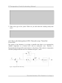
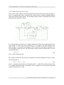
closed-loop diagram similar to the one illustrated in Figure 1, below.
Figure 1 Temperature PI Control Loop
Document Number: 578 Š Revision: 01 Š Page: 3
PI Temperature Control Laboratory Manual
The PI control law implemented in the block diagram of Figure 1 can be formulated as
follows:
V c( t ) = Kp T c_e ( t ) + Ki ⌠
⎮
[3]
⎮ T c_e ( t ) d t
⌡
where the temperature error, Tc_e, can be expressed as shown underneath:
T c_e ( t ) = ( ∆ T c_r ( t ) − ∆ T c( t ) = T c_r ( t ) − T c( t ) )
[4]
The corresponding control loop gains and variables are enumerated in Table 2, below.
Symbol
Description
Unit
Kp
Proportional Gain
V/ºC
Ki
Integral Gain
Tc_r
Reference Chamber Temperature (i.e. Setpoint)
ºC
Tc_e
Chamber Temperature Error
ºC
V/s/ºC
Table 2 PI Control Loop Nomenclature
The sign of the command voltage Vc, as calculated in Equation [3], can then be used to
implement the switching strategy between the plant two possible inputs, that is to say Vh
and Vb. Specifically, the sign of Vc determines whether the chamber needs to heated up (i.e.
Vh is controlled by the PI loop and Vb is set to zero) or cooled down (i.e. Vh is set to zero
and Vb is controlled by the PI loop). Such a switching strategy is formulated by Equation
[5] below:
V c( t )
0 ≤ V c( t )
0
0 ≤ V c( t )
Vh( t ) = {
V
(
t
)
=
{
and
[5]
b
0
V c( t ) < 0
V c( t )
V c( t ) < 0
1. The resulting closed-loop transfer function, TCL(s), of the PI control system is defined in
the Laplace domain as follows:
T c( s )
T CL ( s ) =
[6]
T c_r ( s )
Using the control block diagram [1] and/or Equation [3], derive the expression of TCL(s)
as a function of the system parameters (Kss_c and τc) and the PI controller gains (Kp and
Ki).
Document Number: 578 Š Revision: 01 Š Page: 4
PI Temperature Control Laboratory Manual
Solution:
The resulting closed-loop transfer function can be expressed as:
[s3]
2. TCL(s) should be a second-order system whose denominator can be expressed under the
following standard form:
s 2 + 2 ζ ωn s + ωn
2
[7]
where s is the Laplace operator, ζ the damping ratio, and ωn the undamped natural
frequency.
Derive expressions for the proportional and integral gains, Kp and Ki, as functions of the
system parameters, the damping ratio ζ, and natural frequency ωn.
Solution:
Identifying the coefficients of the two quadratic polynomials of Equations [s3] and [7]
and solving for Kp and Ki results for the proportional gain to:
[s4]
and for the integral gain to:
[s5]
3. For such quadratic systems, it is reminded from classic control theory that the response
peak time, tp, can be expressed as:
π
tp =
[8]
ωn 1 − ζ 2
Likewise the response Percent Overshoot (PO) can be formulated as:
Document Number: 578 Š Revision: 01 Š Page: 5
PI Temperature Control Laboratory Manual
PO = 100 e
⎛−
⎜
⎜⎜
⎝
πζ
⎞
⎟
2 ⎟⎟
1−ζ ⎠
[9]
Derive expressions for the proportional and integral gains, Kp and Ki, as functions of the
system parameters, the damping ratio ζ, and the time to first peak, tp.
Solution:
Solving Equation [8] for ωn, substituting the obtained expression into Equations [s4]
and [s5], and rearranging result for the proportional gain to be such as:
[s6]
and for the integral gain to be expressed by:
[s7]
3.3. Pre-Lab Assignment #3: Controller Design
1. Additionally to exhibiting no steady-state error to a step input, the temperature closedloop response is desired to achieve the following design specifications in terms of peak
time, tp, and damping ratio, ζ:
tp = 20.0 [ s ]
ζ = 0.56
and
[10]
Calculate the proportional and integral gains, Kp and Ki, required to satisfy the design
requirements stated in Equation [10].
Document Number: 578 Š Revision: 01 Š Page: 6
PI Temperature Control Laboratory Manual
Solution:
Evaluating Equation [s6] for the design requirements expressed in Equation [10] and
with the system parameters found in Equations [s1] and [s2] leads to the following
value for Kp:
[s8]
.
Likewise evaluating Equation [s7] for the design requirements expressed in Equation
[10] and with the system parameters found in Equations [s1] and [s2] leads to the
following value for Ki:
[s9]
.
2. What is the desired Percent Overshoot (PO)?
Solution:
The desired ζ, as defined in Equation [10], results in the following Percent Overshoot
(PO):
.
[s10]
3. Finally the designed PI control loop will operate around the following operating
temperature level, Tc_op:
Tc_op = 32.0 [ degC ]
[11]
If the chamber temperature setpoint variation, ∆Tc_r, is a square wave of 2-degreeCelsius amplitude around Tc_op, to what values do you expect the temperature to
overshoot to?
Document Number: 578 Š Revision: 01 Š Page: 7
PI Temperature Control Laboratory Manual
Solution:
With a square wave setpoint variation, ∆Tc_r, of 2 degrees Celsius, the peak-to-peak
signal is 4 degrees. It is reminded that the overshoot is applied to the peak-to-peak
value and added to the reference signal.
Therefore, the temperature response overshoot, Tc_peak, can be expressed for a positive
(i.e. rising) step input as follows:
[s11]
where | | represents the absolute value function.
Evaluating the expression above, the positive overshoot value |Tc_peak| is expected to be
such as:
[s12]
3.4. Pre-Lab Assignment #4: Final Controller Design
The temperature Proportional-plus-Integral (PI) control scheme previously developed and
illustrated in Figure 1, above, is improved in this section to better suit the characteristics of
each of the heating and cooling processes, both composing the HVAC system. Therefore although based on the same standard PI loop, two slightly different control schemes are designed hereafter in order to better accommodate the physical particularities of each process.
As previously defined in Equation [5], it is reminded that the switching logic between the
heating and cooling control loops is still determined by the sign of Vc.
3.4.1. Heating Control Loop
For a more effective heating control loop, the basic PI scheme shown in Figure 1, above, is
complemented with a feed-forward action, an offset voltage, and an integrator anti-windup
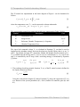
element, as illustrated by the block diagram shown in Figure 2, below.
Document Number: 578 Š Revision: 01 Š Page: 8
PI Temperature Control Laboratory Manual
Figure 2 Heating Control Loop: Active Iff Vc ≥ 0
It is reminded that the heating control loop effectively commands the heater input voltage,
Vh, and is only active if and only if Vc is positive. The basic chamber command voltage Vc
is calculated accordingly to the PI control law formulated in Equation [3]. Also during the
heating process, the blower input voltage remains constant and set to zero, as expressed below:
Vb ( t ) = 0
[12]
where t is the continuous time.
The complete control law for heating, as depicted by the block diagram of Figure 2 above,
can be expressed as:
V h ( t ) = V c( t ) + V h_ff ( t ) + V h_off
[13]
where Vh_off is the heater offset voltage and Vh_ff is the heater feed-forward voltage as
defined by:
V h_ff ( t ) = Kff_h ( T c_r ( t ) − T a )
[14]
with Ta the ambient temperature outside of the chamber, Tc_r the desired chamber
temperature, and Kff_h the heater feed-forward gain.
Feed-forward action is necessary to bring and maintain the chamber temperature to the desired level. It compensates for the standard air cooling in the chamber due to natural heat
Document Number: 578 Š Revision: 01 Š Page: 9
PI Temperature Control Laboratory Manual
dissipation. The PI control system compensates for small variations (e.g. disturbances) from
that operating point.
1. Using the definition of the heater steady-state gain Kss_h, characterize the heater voltage
feed-forward gain Kff_h, as defined in Equation [14].
Hint:
It is reminded that in the steady-state Vh_ff is the voltage required to maintain Tc at the
desired level Tc_r.
Solution:
The heater feed-forward gain can be expressed by:
[s13]
2. From the parameters of the heating transfer function Gh(s) estimated in Reference [3],
calculate the numerical value of Kff_h?
Solution:
Evaluating Equation [s13] with the heater steady-state gain, Kss_h, estimated in
Reference [3] and shown in Equation [s18] of Reference [3] leads to:
[s14]
The heater constant offset voltage, Vh_off, is included in Equation [13] in order to compensate for the halogen lamp deadband. The actuator behaviour, resulting from such a deadband compensation will be more linear around small input voltages. Vh_off has been estimated in Reference [3] as the upper limit of the heating actuator deadzone.
The anti-windup element in the feedback loop stops the integral action when the actuator
saturates to prevent large overshoots in the response. The HVAC heater saturates at Vh_max.
When this limit is reached, the surplus voltage is multiplied by the gain Ka and the result is
removed from the integrator input. The anti-windup element is implemented using a deadzone nonlinearity with a slope of Ka, as shown in Figure 2.
Document Number: 578 Š Revision: 01 Š Page: 10
PI Temperature Control Laboratory Manual
3.4.2. Blowing Control Loop
Likewise for a more effective blowing control loop, the basic PI scheme shown in Figure 1,
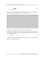
above, is complemented with a constant offset voltage used for actuator deadband compensation and an anti-windup scheme. The resulting control scheme is illustrated by the block
diagram shown in Figure 3, below.
Figure 3 Blowing Control Loop: Active Iff Vc < 0
It is reminded that the blowing (or cooling) control loop effectively commands the blower
input voltage, Vb, and is only active if and only if Vc is negative. The basic chamber command voltage Vc is calculated accordingly to the PI control law formulated in Equation [3].
Also during the cooling process, the heater input voltage remains constant and set to zero,
as expressed below:
Vh ( t ) = 0
[15]
where t is the continuous time.
The complete control law for blowing, as depicted by the block diagram of Figure 3 above,
can be expressed as:
V b ( t ) = V c( t ) + V b_off
[16]
where | | represents the absolute value function and Vb_off is the blower offset voltage. Since
Vc is negative during blowing, the absolute value is required to send a positive command
voltage to the blower (i.e. fan).
Document Number: 578 Š Revision: 01 Š Page: 11
PI Temperature Control Laboratory Manual
The blower constant offset voltage, Vb_off, is included in Equation [16] in order to compensate for the fan deadband. Vb_off has been estimated in Reference [3] as the upper limit of the
fan deadzone.
The blower saturates at Vb_max. Similarly to the heating control loop, the integrator is "turned
off" when Vb_max is reached to prevent large overshoots that can result from the integrator
charging up too much. The same deadzone nonlinearity slope Ka is used.
3.4.3. Final Temperature Control Laws
To summarize and reformulate the previous design considerations, the two actuator input
voltages are completely defined below by Equations [17] and [18].
Using Equations [13] and [15], the heater input voltage is calculated as defined below:
V c( t ) + V h_ff ( t ) + V h_off
0 ≤ V c( t )
Vh( t ) = {
[17]
0
V c( t ) < 0
Likewise using Equations [14] and [16], the blower input voltage is determined as follows:
0
0 ≤ V c( t )
Vb( t ) = {
[18]
V c( t ) + V b_off
V c( t ) < 0
4. In-Lab Session
4.1. System Hardware Configuration
This in-lab session is performed using the NI-ELVIS system equipped with a QNETHVACT board and the Quanser Virtual Instrument (VI) controller file
QNET_HVAC_Lab_06_PI_Control.vi. Please refer to Reference [2] for the setup and
wiring information required to carry out the present control laboratory. Reference [2] also
provides the specifications and a description of the main components composing your
system.
Before beginning the lab session, ensure the system is configured as follows:
 QNET HVACT module is connected to the ELVIS.
 ELVIS Communication Switch is set to BYPASS.
 DC power supply is connected to the QNET HVAC Trainer module.
Document Number: 578 Š Revision: 01 Š Page: 12
PI Temperature Control Laboratory Manual

The 4 LEDs +B, +15V, -15V, +5V on the QNET module should be ON.
4.2. Experimental Procedure
Please follow the steps described below:
Step 1. Read through Section 4.1 and go through the setup guide in Reference [2].
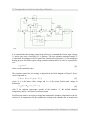
Step 2. Open the VI controller file QNET_HVAC_Lab_06_PI_Control.vi. You should
obtain a front panel similar to the one shown in Figure 4, below. The default sampling
rate for the implemented digital controller is 250 Hz. However, you can adjust it to
your system's computing power. Please refer to Reference [2] for a complete system's
description. The chamber temperature, directly sensed by the thermistor, is plotted on
a chart (in red) as well as displayed in a Numeric Indicator located in the Chamber
Temperature front panel box. The values are in degrees Celsius.
Figure 4 Front Panel Used for the QNET-HVACT Temperature Control Laboratory
Step 3. The vertical toggle switch in the Setpoint Type box allows you to choose
Document Number: 578 Š Revision: 01 Š Page: 13
PI Temperature Control Laboratory Manual
between a Square Wave or a Constant type of reference temperature, Tc_r. Ensure that
it is set to the Square Wave position. The temperature setpoint is also plotted on the
front panel chart (in blue). Use the Numeric Controls of the Setpoint Properties box
to set the chamber operating temperature, Tc_op, to 32 °C (as expressed in Equation
[11]), the square wave Amplitude to -2 °C, and Period to 150 seconds. Specifically
the setpoint properties parameters are expressed in Table 3, below.
Signal Type
Tc_op [°C]
Amplitude [°C]
Period [s]
Square Wave
32.0
-2.0
150.0
Table 3 Temperature Setpoint Parameters
Step 4. When you first open the QNET_HVAC_Lab_06_PI_Control.vi controller file, the
default controller gains are not yet tuned. An example of "untuned" controller
parameters is provided in Table 4, below.
Kp
Ki
Kff_h
Ka
Vh_off
Vb_off
[V/°C]
Ta
[°C]
[V/°C]
[V/s/°C]
[°C/V]
[V]
[V]
3.50
1.50
0.00
22.5
0.0
0.0
0.0
Table 4 "Untuned" Controller Parameters
Run the LabVIEW VI (Ctrl+R) to start the controller. Ensure the initially green
START push button is pressed and shown as a red STOP button to activate the
controller. This button can be used to pause the controller execution. With the control
action active, the chamber temperature should now go up and down to roughly track
the desired square wave setpoint. You should obtain an "untuned" temperature
response similar to the one depicted in Figure 4, above. After a few periods, you can
stop the VI by pressing the red EXIT button on the front panel.
Step 5. Using the Numeric Controls of the Controller Gains box, you should enter the
system controller gains, namely Kp, Ki and Kff_h, that you have calculated in the prelab section. Also enter the ambient temperature (Ta, in °C) present outside of the
HVAC chamber. Set the value of Ka to 0.0 °C/V, which effectively turns off the
integral anti-windup element in the feedback system. Finally the deadband
compensation parameters, Vh_off and Vb_off, should also be properly set to the values
that you estimated in Reference [3]. Do so by using the Numeric Controls of the
Deadband Compensation box on the front panel. Summarize your final tuned
controller parameters by filling up Table 5 as shown below.
Document Number: 578 Š Revision: 01 Š Page: 14
PI Temperature Control Laboratory Manual
Kp
[V/°C]
Ki
[V/s/°C]
Kff_h
[V/°C]
Ta
[°C]
0.57
0.37
0.07
22.5
Ka
[°C/V]
Vh_off
[V]
Vb_off
[V]
0.5
0.8
12.6
Table 5 Tuned Controller Parameters
Step 6. Start the controller by running the LabVIEW VI (Ctrl+R) in order to try your
calculated gains on the actual system. The software applies square wave temperature
setpoints to the closed-loop control system and plots both setpoint and actual chamber
temperature over a 350-second time range. Observe the way the system switches
between the two actuators (i.e. lamp and fan) in order for the chamber temperature to
track the desired square wave setpoint around the operating level Tc_op.
Step 7. Let the system run until you have plotted on the chart the temperature response
to 2 heating steps and to 2 cooling steps (at least the overshoot and peak time part of
it).
Step 8. Make a screen capture of the obtained step response plot and join a printout to
your report.
Document Number: 578 Š Revision: 01 Š Page: 15
PI Temperature Control Laboratory Manual
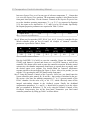
Solution:
Figure 5, below, illustrates typical experimental results from the designed closedloop system by showing the actual temperature response tracking a desired square
wave setpoint. The anti-windup element is not being used in this closed-loop
response.
Figure 5 Desired And Actual Temperature Signals not using Integrator Anti-windup
Step 9. Does the closed-loop system track the desired square wave setpoint accurately?
Is there any steady-state error? Comment on the symmetry (or lack of) of the
temperature response between heating and blowing steps. Explain.
Solution:
The system tracks the desired temperature square wave with considerable steadystate error, which is chiefly due to the integrator charging up too much and causing
overshoot and the various nonlinearities of the system not accounted for in the
model.
As expected, the system has an asymmetrical response: heating behaves differently
than cooling (i.e. blowing). Although assumed otherwise in the controller gain
calculations, a different process/plant is at play in each case.
Document Number: 578 Š Revision: 01 Š Page: 16
PI Temperature Control Laboratory Manual
Step 10. Set the value of Ka to 0.2 °C/V, which corresponds to slope of the integral antiwindup deadzone to 0.2 °C/V, and keep the same values for the other control
parameters entered in Table 5. Start the controller by running the LabVIEW VI
(Ctrl+R) in order to try your calculated gains on the actual system using the antiwindup element. Observe the effects on the response of having an anti-windup
element. Then, adjust Ka to improve the response and enter the tuned parameter in
Table 5, above.
Step 11. Let the system run until you have plotted on the chart the temperature response
to 2 heating steps and to 2 cooling steps (at least the overshoot and peak time part of
it).
Step 12. Make a screen capture of the obtained step response plot and join a printout to
your report.
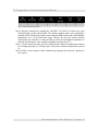
Solution:
Figure 6, below, illustrates typical experimental results from the designed closedloop system using the anti-windup element by showing the actual temperature
response tracking a desired square wave setpoint.
Figure 6 Desired And Actual Temperature Signals using Integrator Anti-windup
Step 13. You should now measure and determine your system performance from the
Document Number: 578 Š Revision: 01 Š Page: 17
PI Temperature Control Laboratory Manual
actual response plot, as displayed on the VI Front Panel. Do so by using the Graph
Palette located on top of the Chart top left corner. Fill up Table 6 as shown below.
You should have plotted two iterations of both step types, i.e. heating and blowing.
First measure the corresponding Percent Overshoot, PO, and peak time, tp, for all 4
step responses as specified in Table 6. Tc_peak is the overshoot value. Then take the
average of PO and tp over the 2 iterations of each step type. Finally, combine and
average the results of both step types. What are your final values for PO and tp?
Step Type
Iteration #
Tc_peak [ºC]
PO [%]
tp [s]
Heating
1
34.05
1.25
12.5
2
34.05
1.25
12.5
Average:
X
1.25
0.0
1
30.15
3.75
18.5
2
30.15
3.75
20.0
Average:
X
3.75
0.0
X
2.50
0.0
Blowing
Average Values:
Table 6 Step Response Actual Performance
Step 14. Do the measured Percent Overshoot and peak time meet the required
specifications? Explain your observations.
Solution:
As measured and calculated in Table 6 above, the measured peak time is globally
about 15.9 seconds on average and the Percent Overshoot is approximately to
2.5%. Therefore the tp of the actual system is close to the desired value in [10] and
the resulting PO of the device is considerably less than the required value specified
in [s10], primarily due to the integrator anti-windup mechanism. Consequently, the
required design specifications are met.
Step 15. If the design requirements defined by Equation [10] are still not satisfied, you
should manually fine tune the controller parameters of Table 5 until the response
performance improves to the desired level. Include in your laboratory report your
final tuning parameters, experimental plots and results, as well as the measured
system performance criteria satisfying the specifications.
Step 16. Once all your experimental results are obtained, shut off the PROTOTYPING
POWER BOARD switch and the SYSTEM POWER switch at the back of the ELVIS
unit. Unplug the module AC cord. Then, stop the VI by pressing the red EXIT button.
Document Number: 578 Š Revision: 01 Š Page: 18