1
Quanser NI-ELVIS Trainer (QNET) Series:
QNET Experiment #03:
Gantry Control
Rotary Pendulum (ROTPEN) Gantry
Trainer
Student Manual
QNET Gantry Laboratory Manual
Table of Contents
1. Laboratory Objectives.........................................................................................................1
2. References............................................................................................................................1
3. ROTPEN Plant Presentation................................................................................................1
3.1. Component Nomenclature...........................................................................................1
3.2. ROTPEN Plant Description.........................................................................................2
4. Pre-Lab Assignments...........................................................................................................3
4.1. Pre-Lab Assignment #1: Open-Loop Modeling..........................................................3
4.1.1. Exercise: Kinematics............................................................................................5
4.1.2. Exercise: Potential Energy...................................................................................6
4.1.3. Exercise: Kinetic Energy......................................................................................7
4.1.4. Exercise: Lagrangian of System...........................................................................7
4.1.5. Exercise: Euler-Lagrange EOM...........................................................................9
4.1.6. Exercise: Euler-Lagrange Matrix Form.............................................................10
4.2. Pre-Lab Assignment #2: Finding the Linear State-Space Model..............................11
4.2.1. Exercise: Linearizing EOM................................................................................12
4.2.2. Exercise: Solving for EOM Acceleration Terms...............................................13
4.2.3. Exercise: Finding State-Space Model................................................................14
4.2.4. Exercise: Adding Actuator Dynamics................................................................16
4.3. Pre-Lab Assignment #3: Calculating the Inertia and Center of Mass of the Pendulum
...........................................................................................................................................17
4.3.1. Exercise: Calculating Center of Mass................................................................19
4.3.2. Exercise: Calculating Moment of Inertia...........................................................22
4.4. Control Design...........................................................................................................23
4.4.1. Controllability....................................................................................................23
4.4.2. Linear Quadratic Regulator................................................................................25
4.4.3. Gantry Control Specifications............................................................................26
5. In-Lab Session...................................................................................................................27
5.1. System Hardware Configuration................................................................................27
5.2. Experimental Procedure.............................................................................................28
Document Number: 576 Revision: 01 Page: i
QNET Gantry Laboratory Manual
1. Laboratory Objectives
In industry, the crane is often used to transport items from one place to another. The gantry
experiment involves developing a control system for a crane travelling on a moving
platform. In this case, the crane is represented by the suspended pendulum and the rotary
arm behaves as the moving platform that transports the crane at different locations. The
problem is to develop a controller that enables the platform, or in this case the arm of the
rotary pendulum system, to track a commanded position while minimizing the motions of
the crane, or pendulum, as it is being transported.
In this laboratory, the equations representing the motions of the rotary pendulum will be
derived using a technique known as Lagrange. The resulting nonlinear dynamics are then
then linearized and converted to a state-space model. The linear state-space representation
of a system is different than Laplace and is used more prominently in the control research
field. The obtained model is then used to design a closed-loop controller using the LinearQuadratic Regulator technique. It is used to minimize or dampen the movements of the
suspended pendulum while the rotary arm tracks the reference angle given. Practically
speaking, the algorithm developed regulates the movements of the gantry and keeps the
crane steady in the vertical down position such that items can be transported in a safely.
Regarding Gray Boxes:
Gray boxes present in the instructor manual are not intended for the students as they
provide solutions to the pre-lab assignments and contain typical experimental results
from the laboratory procedure.
2. References
[1] NI-ELVIS User Manual.
[2] QNET-ROTPEN User Manual.
3. ROTPEN Plant Presentation
3.1. Component Nomenclature
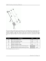
As a quick nomenclature, Table 1, below, provides a list of the principal elements
composing the Rotary Pendulum (ROTPEN) Trainer system. Every element is located and
identified, through a unique identification (ID) number, on the ROTPEN plant represented
Revision: 01 Page: 1
QNET Gantry Laboratory Manual
in Figure 1, below.
ID #
Description
Description
ID #
1
DC Motor
3
Arm
2
Motor/Arm Encoder
4
Pendulum
Table 1 ROTPEN Component Nomenclature
Figure 1 ROTPEN System
3.2. ROTPEN Plant Description
The QNET-ROTPEN Trainer system consists of a 24-Volt DC motor that is coupled with
an encoder and is mounted vertically in the metal chamber. The L-shaped arm, or hub, is
connected to the motor shaft and pivots between ±180 degrees. At the end of the arm there
is a suspended pendulum attached. The pendulum angle is measured by an encoder.
Revision: 01 Page: 2
QNET Gantry Laboratory Manual
4. Pre-Lab Assignments
This section must be read, understood, and performed before you go to the laboratory
session.
4.1. Pre-Lab Assignment #1: Open-Loop Modeling
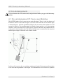
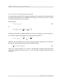
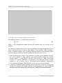
The ROTPEN plant is free to move in two rotary directions. That is, it has two degrees of
freedom or 2 DOF. As described in Figure 2, the arm rotates about the Y0 axis and its angle
is denoted by the θ while the pendulum attached to the arm rotates about another axis and
its angle is called α. The pendulum angle is defined as being positive, α>0, when rotating
clockwise. Thus as the arm moves in the positive clockwise direction, the pendulum moves
in the positive clockwise direction. The shaft of the DC motor is connected to the arm pivot
and the input voltage of the motor is the control variable.
Figure 2 Rotary Pendulum System
In this pre-lab exercise, the raw nonlinear mathematical model that represents the motions
of the arm and the pendulum is developed. Given nonetheless are the nonlinear dynamics
Revision: 01 Page: 3
QNET Gantry Laboratory Manual
between the angle of the arm, θ, the angle of the pendulum, α, and the torque applied at the
arm pivot, τoutput.
2
2
Mp g lp r cos( θ( t ) ) α( t )
d2
θ
(
t
)
=
−
2
dt2
( Mp r 2 cos( θ( t ) )2 + Jeq ) Jp + Mp lp Jeq
2
d
2
Jp Mp r cos( θ( t ) ) sin( θ( t ) ) ⎛⎜⎜ θ( t ) ⎞⎟⎟
Jp τoutput + Mp lp τoutput
d
t
⎝
⎠ +
+
2
2
2
2
( Mp r cos( θ( t ) ) + Jeq ) Jp + Mp lp Jeq ( Mp r2 cos( θ( t ) )2 + Jeq ) Jp + Mp lp Jeq
2
[1]
lp Mp ( Jeq g + Mp r g cos( θ( t ) ) ) α( t )
d2
α
(
t
)
=
−
2
dt 2
( Mp r 2 cos( θ( t ) )2 + Jeq ) Jp + Mp lp Jeq
2
2
2
d
lp Mp r sin( θ( t ) ) Jeq ⎛⎜⎜ θ( t ) ⎞⎟⎟
lp Mp r τoutput cos( θ( t ) )
⎝ dt
⎠
−
+
2
2
( Mp r2 cos( θ( t ) )2 + Jeq ) Jp + Mp lp Jeq ( Mp r2 cos( θ( t ) )2 + Jeq ) Jp + Mp lp Jeq
where the torque generated at the arm pivot from the motor voltage, Vm, is
d
Kt ⎛⎜⎜ Vm − Km ⎛⎜⎜ θ( t ) ⎞⎟⎟ ⎞⎟⎟
⎝ dt
⎠⎠
τoutput = ⎝
Rm
.
[2]
The ROTPEN model parameters used in [1] and [2] are defined in Table 2.
Symbol
Mp
Description
Mass of the pendulum assembly (weight and link
combined).
lp
Length of pendulum center of mass from pivot.
Lp
Total length of pendulum.
r
Length of arm pivot to pendulum pivot.
Jm
Motor shaft moment of inertia.
Marm
g
Value
Unit
kg
0.027
m
0.191
m
0.06668
m
3.00E-005
kg⋅m2
Mass of arm.
0.028
kg
Gravitational acceleration constant.
9.810
m/s2
Revision: 01 Page: 4
QNET Gantry Laboratory Manual
Symbol
Jeq
Description
Equivalent moment of inertia about motor shaft
pivot axis.
Value
Unit
kg⋅m2
1.23E-004
Jp
Pendulum moment of inertia about its pivot axis.
Beq
Arm viscous damping.
0.000
N⋅m/(rad/s)
Bp
Pendulum viscous damping.
0.000
N⋅m/(rad/s)
Rm
Motor armature resistance.
3.30
Ω
Kt
Motor torque constant.
0.02797
N⋅m/A
Km
Motor back-electromotive force constant.
0.02797
V/(rad/s)
kg⋅m2
Table 2 ROTPEN Model Nomenclature
Note that the pendulum center of mass, lp, and the moment of inertia parameter, Jp, are not
given because they will be calculated later in pre-lab exercise. Also viscous damping,
which is a friction that opposes the velocity at which the structure is moving, is regarded as
being negligible.
The following exercises build the rotary pendulum model incrementally. The first step is
finding the kinematics of the center-of-gravity of the pendulum. In the second and third
step, these are used to compute the potential and kinetic energy of the system. The fourth
step introduces the principle of Lagrange and uses Euler-Lagrange equations to calculate
the nonlinear equations of motion, or EOMs, that are given in [1].
4.1.1. Exercise: Kinematics
Consider the pendulum a point mass solid object. Find the forward kinematics of the
pendulum center of gravity, COG, with respect to the base frame o0x0y0. That is, express the
position, xp and yp, and the velocity, xdp and ydp, of the pendulum COG in terms of the
angles θ and α. The height between the pendulum pivot and the base of the arm is h = 0.127
m.
Revision: 01 Page: 5
QNET Gantry Laboratory Manual
Solution:
The kinematics of the pendulum COG relative to the base coordinate system o0x0y0 is
[s1]
and the velocity components are found by taking the derivative of [s1] with respect to
time
.
4.1.2. Exercise: Potential Energy
Express the total potential energy, VT(α), of the rotary pendulum system. There is no elastic
component in the system, therefore the energy that can be stored for movement is from
gravity. The gravitational potential energy depends on the vertical position of the pendulum
COG.
Solution:
The gravitational potential energy is dependent on the vertical position of the
pendulum COG. Thus using expression yp from the above exercise, the total potential
energy of the system is
resulting in
.
Revision: 01 Page: 6
QNET Gantry Laboratory Manual
4.1.3. Exercise: Kinetic Energy
Find the total kinetic energy, Tt, of the ROTPEN system. This includes the rotational kinetic
energy of the arm and the pendulum as well as the translational kinetic energy of the
pendulum COG. It is reminded that the arm's equivalent moment of inertia at the pivot is Jeq
and the inertia of the pendulum at its rotating pivot is Jp.
Solution:
The total kinetic energy of the system can be described is
.
The rotational kinetic energy of the arm is
,
where Jeq is the equivalent inertia of the arm at the pivot. Likewise, the rotational
kinetic energy of the pendulum is
,
where Jp is the moment of inertia of the pendulum about the pendulum's pivot axis.
Lastly, the translational kinetic energy of the pendulum center of mass is
.
Note that the parameters used in the above expressions are given and described in
Table 2.
4.1.4. Exercise: Lagrangian of System
The Lagrangian of a system is
L = Tt − Vt
[3]
where Tt is the total kinetic energy of the system, calculated in Exercise 4.1.3, and Vt is the
total potential energy of the system, calculated in Exercise 4.1.2. The Lagrangian of a
system is the difference between the total kinetic energy of the system and its total potential
energy. The Euler-Lagrange equations of motions is a set of differential equations that
describe the motions of a system and it is generated from the Lagrangian. The equations of
Revision: 01 Page: 7
QNET Gantry Laboratory Manual
motion is a mathematical model that represents an actual real-world system.
Q1. Substitute the generalized coordinates qi
q1 = θ
q =α
and 2
in the kinetic energy, Tt, and potential energy, Vt, expressions found in Exercise 4.1.3
and 4.1.2.
Q2. Compute the Lagrangian
L( q ) = Tt( q ) − Vt( q )
where
q = [ q1, q2 ]
T
.
That is, calculate the Lagrangian of the rotary pendulum system in terms of the qi
coordinates.
Q3. Format the solution of L(q) into the following quadratic structure
d
d
⎛ d2
⎞
⎛ d2
⎞
⎛
⎞
⎛
⎞
⎜
⎟
d11( q1 ) ⎜ 2 q1( t ) ⎟ + 2 d12( q1, q2 ) ⎜⎜ q2( t ) ⎟⎟ ⎜⎜ q1( t ) ⎟⎟ + d22( q2 ) ⎜⎜ 2 q2( t ) ⎟⎟ − Vt( q) =
⎜⎝ dt
⎟⎠
⎜
⎟⎠
d
t
d
t
⎠
⎝
⎠⎝
⎝ dt
τoutput
[4]
and enter the inertia terms d11(q1), d12(q), and d22(q2), and the potential energy term, Vt(q),
into Table 3 below. Note that τouput is the DC motor torque defined above in [2].
Inertia Term
Expression
d11(q1) =
d12(q) =
d22(q2) =
Vt(q2) =
Table 3 Lagrangian Inertia Terms
Revision: 01 Page: 8
QNET Gantry Laboratory Manual
4.1.5. Exercise: Euler-Lagrange EOM
The Euler-Lagrange equations of motion are calculated from the Lagrangian of a system
using
⎛⎜ ∂ 2
⎞⎟ ⎛ ∂ ⎞
[5]
⎜⎜ ∂t ∂qdot L ⎟⎟ − ⎜⎜ ∂q L ⎟⎟ = Qi
i ⎠
⎝
⎝ i ⎠
where for an n degree-of-freedom structure i = {1,..,n} and Qi is called generalized force.
In the rotary pendulum system, the generalized forces are
d
Q1 = τoutput − Beq ⎛⎜⎜ θ( t ) ⎞⎟⎟
⎝ dt
⎠
d
Q2 = −Bp ⎛⎜⎜ α( t ) ⎞⎟⎟
⎝ dt
⎠.
However, since the viscous damping of the arm, Beq, and the pendulum, Bp, are regarded as
being negligible, the generalized forces become simply Q1 = τoutput and Q2 = 0. With that
information, applying [5] to the Lagrangian expression in [4] and performing some
manipulation gives
2
d
d
d
⎛ d2
⎞
⎛ d2
⎞
d11 ⎜⎜ 2 q1( t ) ⎟⎟ + d12 ⎜⎜ 2 q2( t ) ⎟⎟ + c111⎛⎜⎜ q1( t ) ⎞⎟⎟ + ( c121 + c112) ⎛⎜⎜ q1( t ) ⎞⎟⎟ ⎛⎜⎜ q2( t ) ⎞⎟⎟
⎜⎝ dt
⎟⎠
⎜⎝ dt
⎟⎠
⎠
⎝ dt
⎠
⎝ dt
⎠ ⎝ dt
2
d
+ c122⎛⎜⎜ q2( t ) ⎞⎟⎟ + φ1 = τoutput
⎝ dt
⎠
2
d
d
d
⎛ d2
⎞
⎛ d2
⎞
d12 ⎜⎜ 2 q1( t ) ⎟⎟ + d22 ⎜⎜ 2 q2( t ) ⎟⎟ + c211⎛⎜⎜ q1( t ) ⎞⎟⎟ + ( c221 + c212) ⎛⎜⎜ q1( t ) ⎞⎟⎟ ⎛⎜⎜ q2( t ) ⎞⎟⎟
⎜⎝ dt
⎟⎠
⎜⎝ dt
⎟⎠
⎠
⎝ dt
⎠
⎝ dt
⎠ ⎝ dt
[6]
2
d
+ c222⎛⎜⎜ q2( t ) ⎞⎟⎟ + φ2 = 0
⎝ dt
⎠
where for i = {1,2}, j = {1,2}, and k = {1,2}, dij is the inertia terms previously calculated,
cijk are called Christoffel symbols, and φk is a function of the potential energy. The
Christoffel symbols are
1 ∂
1 ∂
1 ∂
cijk = ⎛⎜
d kj ⎞⎟ + ⎛⎜
d ki ⎞⎟ − ⎛⎜
d ⎞⎟
[7]
2 ⎜ ∂qi ⎟ 2 ⎜ ∂qj ⎟ 2 ⎜ ∂qk ij ⎟
⎝
⎠
⎝
⎠
⎝
⎠
and
φk( q ) =
∂
V (q)
∂qk t
[8]
.
Revision: 01 Page: 9
QNET Gantry Laboratory Manual
Complete the Table 4 below by finding the Christoffel symbols using [7] and φk using [8].
Parameter
Value
Parameter
Value
c111 =
c112 =
c121 = 0
c212 = 0
c211 = 0
c212 = 0
c221 =
c222 = 0
φ1 = 0
φ2 =
Table 4 Lagrangian Christoffel symbols and φk
4.1.6. Exercise: Euler-Lagrange Matrix Form
The equations of motion of the rotary pendulum have now been found. The matrix form of
the Euler-Lagrangian equations of motion in [6] is commonly seen as
d
d
⎛⎜ d 2
⎞
D( q ) ⎜ 2 q( t ) ⎟⎟ + C⎛⎜⎜ q, q( t ) ⎞⎟⎟ ⎛⎜⎜ q( t ) ⎞⎟⎟ + g( q( t ) ) = τ
[9]
⎜⎝ d t
⎟⎠
⎝ dt
⎠ ⎝ dt
⎠
where for a 2 DOF system
⎡d 11( q1 ) d 21( q ) ⎤⎥
D( q ) = ⎢⎢
⎥
⎢⎣ d 21( q ) d 22( q2 )⎥⎦
,
g( q( t ) ) = [ φ1( q( t ) ), φ2( q( t ) ) ]
τ = [ τoutput , 0 ]
T
,
T
,
and C(q,q_dot) is the matrix that includes the Christoffel symbols in Table 4. Substitute the
expression calculated from dij in Table 3 along with cijk and φk in Table 4 into the EulerLagrange expression in [6] and map it to the matrix form shown in [9]. Fill out the matrices
below in Table 5.
Revision: 01 Page: 10
QNET Gantry Laboratory Manual
Matrix
Value
D( q( t ) )
d
C⎛⎜⎜ q( t ), q( t ) ⎞⎟⎟
dt
⎝
⎠
g( q( t ) )
Table 5 Euler-Lagrangian Matrices
4.2. Pre-Lab Assignment #2: Finding the Linear StateSpace Model
The general state model of a time-invariant linear continuous-time dynamical system is
d
x( t ) = A x( t ) + B u( x )
dt
[10]
y( t ) = C x( t ) + D u( x )
where x(t) is the n-dimensional state, and for an r-input and m-output system A∈ℜn×n,
B∈ℜn×r, C∈ℜm×n, and D∈ℜm×r are constant matrices. The goal of this section is to find the
linear state-space model of the rotary pendulum system. In particular, the goal is to
calculate the A and B matrices. Before going through the actual exercise, an overview of the
process of attaining the model will be given.
The mathematical model of the rotary pendulum found in [9] is nonlinear. Therefore [9]
must be linearized about a operating point in order to fit the system into the state-space
from shown in [10].
Revision: 01 Page: 11
QNET Gantry Laboratory Manual
4.2.1. Exercise: Linearizing EOM
Consider a continuous, nonlinear two-variable function f(x,y) that is to be linearized about
the operating point (xo,yo). The linearization is calculated as follows
∂
∂
fl( x, y ) = f( xo, yo ) + ⎛⎜
f( xo, yo ) ⎞⎟ ( x − xo ) + ⎛⎜
f( x , y ) ⎞⎟ ( y − yo )
⎜ ∂xo
⎟
⎜ ∂yo o o ⎟
⎝
⎠
⎝
⎠
.
The linearized function fl(x,y) is an approximation of the nonlinear function f(x,y) and this
approximation only holds in a region about the operating point. That is, fl(x,y) ≈ f(x,y) when
(x-xo,y-yo)∈C, where C is a two-dimensional region about the origin.
The linearized Euler-Lagrange equation can be given by
d
d
⎛ d2
⎞
Dl( q ) ⎜⎜ 2 q( t ) ⎟⎟ + Cl⎛⎜⎜ q, q( t ) ⎞⎟⎟ ⎛⎜⎜ q( t ) ⎞⎟⎟ + gl( q ) = τ
⎜⎝ d t
⎟⎠
⎝ dt
⎠ ⎝ dt
⎠
[11]
where Dl(q) and Cl(q,q_dot) are the linearized inertia and Christoffel matrices and gl(q) is
the linearized g(q). In the case of the ROTPEN system, the linearized mathematical model
represents the motions of the real physical system only about the point where the angles
were linearized.
Linearize each element of the D(q) and C(q,q_dot) matrices as well as the vector g(q)
about the operating point
xo = [ 0, 0, 0, 0 ]T
and record the results in Table 6.
Matrix
Value
Dl( q( t ) )
d
Cl⎛⎜⎜ q( t ), q( t ) ⎞⎟⎟
dt
⎝
⎠
gl( q( t ) )
Table 6 Linearized Lagrangian Matrices
Revision: 01 Page: 12
QNET Gantry Laboratory Manual
4.2.2. Exercise: Solving for EOM Acceleration Terms
The system has now been linearized and is more easily manageable. The linearized EulerLagrange equations of motions in [11] must be solved for q_ddot, such that
[ -1 ]
[ -1 ]
[ -1 ]
d
d
d2
q( t ) = −Dl( q ) Cl⎛⎜⎜ q, q( t ) ⎞⎟⎟ ⎛⎜⎜ q( t ) ⎞⎟⎟ − Dl( q ) gl( q ) + Dl( q ) τ
[12]
2
dt
⎝ dt
⎠ ⎝ dt
⎠
.
Calculate the solution of [12] from the answer found in Exercise 4.2.1 and structure the
resulting vector in the following two-equation form
∂2
q = a1 q2 + b1 τoutput
∂t 2 1
[13]
∂2
q = a2 q2 + b2 τoutput
∂t 2 2
,
where a1, a2, b1, and b2 are all real number constants. Record the parameters in Table 7.
Solution Parameter Expression
a1
a2
b1
b2
Table 7 Linearized Lagrange Solution Parameters
Revision: 01 Page: 13
QNET Gantry Laboratory Manual
4.2.3. Exercise: Finding State-Space Model
At this point the nonlinear Euler-Lagrange equations of motions have been linearized about
the origin and solved for the acceleration of the angles q1_ddot and q2_ddot. It is now
ready to be placed in the state-space form.
Define the state
x = [ x1, x2, x3, x4 ]
T
[14]
as
T
d
d
x( t ) := ⎡⎢⎢ q1( t ), q2( t ), q1( t ), q2( t ) ⎤⎥⎥
dt
dt
⎣
⎦ .
Recall the generalized coordinates definitions used for the Lagrange: q1(t)=θ(t) and q2(t) =
α(t). The state defined with respect to the rotary pendulum angles are
∂
∂
x4 = α
x1 = θ x2 = α x3 = ∂t θ
∂t .
,
,
, and
Substitute the state defined in [14] into the Lagrange solution computed in [13] and place
the answer in the single-input linear state-space representation
d
x( t ) = A x( t ) + B u( x )
[15]
dt
where A is a real 4×4 matrix, B is a real 4×1 constant matrix, and the control input is the
torque being applied by the motor, u(x) = τoutput(x). Enter the resulting state-space matrices
in Table 8.
Revision: 01 Page: 14
QNET Gantry Laboratory Manual
State-Space Matrix
Expression
A
B
C
⎡⎢ 1
⎢⎢ 0
⎢⎢
⎢⎢ 0
⎣0
D
⎡⎢
⎢⎢
⎢⎢
⎢⎢
⎣
0
1
0
0
0
0
1
0
0⎤
⎥
0⎥⎥
⎥
0⎥⎥
1⎥⎦
0⎤
⎥
0⎥⎥
⎥
0⎥⎥
0⎥⎦
Table 8 Linear State-Space Matrices
The 4×4 matrix C and the 4×1 matrix D in the state model equation
y( t ) = C x( t ) + D u( x )
are given in Table 8. It is assumed from the rank of C that all states are being measured by
sensors. Although in actuality the position angles θ and α are measured by encoders and the
speed of these angles is calculated using an observer. The observer differentiates the angle
and removes any high-frequency components using a low-pass filter. Thus from a controls
Revision: 01 Page: 15
QNET Gantry Laboratory Manual
point of view, the output equation should be y = [x1,x2]T and there should be an observer
that estimates the states x3 and x4. The controller designed later would then be in the form u
= -Kxest and not u = -Kx.
4.2.4. Exercise: Adding Actuator Dynamics
The state equations developed in the last exercise are relative to the torque being applied at
the motor shaft. The torque, however, is not controlled by the computer directly and is,
instead, a result of the voltage being given to the DC motor. The torque generated at the
arm pivot from the motor voltage, Vm, is
d
Kt ⎛⎜⎜ Vm − Km ⎛⎜⎜ θ( t ) ⎞⎟⎟ ⎞⎟⎟
⎝ dt
⎠⎠
τoutput = ⎝
Rm
.
Re-define the state-space equation [15] in terms of u(x) = Vm and write the new matrices in
Table 9.
Revision: 01 Page: 16
QNET Gantry Laboratory Manual
State-Space Matrix
Expression
A
B
Table 9 State-Space Matrices in terms of Vm
4.3. Pre-Lab Assignment #3: Calculating the Inertia and
Center of Mass of the Pendulum
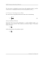
The free-body diagram of the pendulum used in the QNET rotary pendulum system is
shown in Figure 3.
Revision: 01 Page: 17
QNET Gantry Laboratory Manual
Figure 3 Pendulum Free-Body Diagram
The circle in the top-right corner represents the axis of rotation that goes into the page. The
pendulum assembly is a rigid body that is composed of two bodies: the pendulum link, Mp1,
and the pendulum weight, Mp2, located at the end of the link. The mass and length
parameters depicted in Figure 3 that are needed for this exercise are given below in Table
10.
Symbol
Description
Value
Unit
Mp1
Mass of the pendulum link.
0.008
kg
Mp2
Mass of the pendulum weight.
0.019
kg
Lp1
Length of pendulum link.
0.171
m
Lp2
Length of pendulum weight.
0.019
m
lp
Length of pendulum center of mass from pivot.
0.153
m
Jp
Pendulum moment of inertia about its pivot axis.
6.98E-004
kg⋅m2
Table 10 Pendulum Parameters for Exercise 4.3
Revision: 01 Page: 18
QNET Gantry Laboratory Manual
The first exercise is calculating the center of mass of the pendulum assembly, lp, and the
second exercise is computing the moment of inertia of the pendulum system, Jp.
4.3.1. Exercise: Calculating Center of Mass
The center of mass of a rigid body in the form of a beam can be calculated using
⌠
⎮p x d x
xcm = ⌡
⌠
⎮p d x
⌡
where p is the density of the body.
[16]
Express the center of mass of the pendulum link, xcm1, and the pendulum weight, xcm2, in
terms of Lp1, Lp2, Mp1, and Mp2. These variables are all shown in Figure 3. The uniform
density of the link is
Mp1
p1 =
Lp1
and the uniform density of the pendulum weight is
Mp2
p2 =
Lp2
.
Revision: 01 Page: 19
QNET Gantry Laboratory Manual
Solution:
The center of mass of the pendulum link using [16] begins with
.
Since the density of the pendulum link, p1, is uniform the denominator and numerator
constants cancel each other out. As expected, the integration results in half the length
of the rod,
.
Similarly the CM of the pendulum mass from the axis of rotation is
and results in
which simplifies into the more intuitive expression
.
The pendulum is composed of two different bodies each with their own CM. The center of
mass of the body as a whole can be calculated and is useful when the pendulum is to be
considered as a single rigid object. The center of mass of a composite object that contains n
Revision: 01 Page: 20
QNET Gantry Laboratory Manual
bodies can be calculated using
∑ xi mi
xcm =
i
[17]
∑ mi
i
where xi is the known center of mass of body i and mi is the mass of body i.
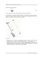
If the ROTPEN is considered a single rigid body, its CM would be as shown in Figure 4
and not as two separate bodies in Figure 3. The total mass of the pendulum assembly is Mp
and the total length is Lp, both are quantified in Table 2.
Figure 4 Free body diagram of pendulum considered a
single rigid body.
1. Express the center of mass of the pendulum assembly in terms of the CM of the
pendulum link, xcm1, and the CM of the pendulum mass, xcm2, using expression [17].
2. Calculate the numerical answer using the mass and length parameters given in Table 10
and enter the resulting center of mass, lp, in Table 10. Record the answer for later use
in QNET Laboratory #4 – ROTPEN Inverted Pendulum.
Revision: 01 Page: 21
QNET Gantry Laboratory Manual
Solution:
The center of mass of the pendulum composite from its axis of rotation is expressed as
where xcm1 is the CM of the pendulum link and xcm2 is the CM of the pendulum mass.
Expanding the summation and substituting the parameters given in Table 10 gives the
numerical answer of
.
4.3.2. Exercise: Calculating Moment of Inertia
The moment of inertia J of a rigid body is expressed as
J=⌠
r2 dm
⎮
[18]
⎮
⌡
where r is the perpendicular distance between the element mass, dm, and the axis of
rotation.
The moment of inertia at the pivot axis of the pendulum is an important parameter for the
gantry experiment because it indicates the tendency of the pendulum, which represents a
crane, to continue swinging. Thus a pendulum with more inertia is more difficult to control
then one with less tendency to continue rotating when the arm ceases to move.
1. Express the moment of inertia of the pendulum Jp in terms of the pendulum link mass,
Mp1, and its length, Lp1, along with the mass of the pendulum weight, Mp2, and the
weight's length, Lp2, using general expression [18] and Figure 3. Hint: Recall from
Exercise 4.3.1 that the pendulum is a composite of two thin rods with the uniform
densities p1 = Mp1/Lp1 and p2 = Mp2/Lp2. The integral can be evaluated by changing the
mass element to the distance differential dm = p*dr, where p is the linear density.
2. Compute the pendulum moment of inertia and enter the result in Table 10. The mass and
length of the pendulum link and the pendulum weight are specified in Table 10. Record
the answer for later use in QNET Laboratory #4 – ROTPEN Inverted Pendulum.
Revision: 01 Page: 22
QNET Gantry Laboratory Manual
Solution:
Applying [18] to the pendulum assembly gives
.
Evaluating the above integral and substituting the above p1 and p2 expressions results
in the pendulum moment of inertia expression
that simplifies to
.
The moment of inertia of the pendulum is given in Table 10 after substituting Mp1,
Mp2, Lp1, and Lp2 listed in Table 10.
4.4. Control Design
The goal of this section is to introduce the notion of controllability of a system and the idea
behind the Linear-Quadratic Regular, or LQR, control technique. This is an introduction to
designing a linear controller in the state-space.
4.4.1. Controllability
Consider this arbitrary system
d
x ( t ) = x2
dt 1
d
x (t) = u
dt 2
.
[19]
Revision: 01 Page: 23
QNET Gantry Laboratory Manual
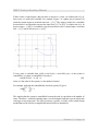
If there exists a control input u that can drive a state x to a vector v in a finite time of t1>0,
then vector v is said to be reachable. For example, Figure 5 is a phase plot of system [19]
when the system begins at an initial state x(0) = [1,1]T. The origin is said to be a reachable
because there is an input that can steer the state from [1,1]T to [0,0]T in a finite time of t1. In
precise terms, v = [0,0] is a reachable vector because there exists a control input u such that
x(0) = [1,1]T can be driven to x(t1) = [0,0]T.
Figure 5 Phase Plot of a System
If every state is reachable then (A,B) is said to be a controllable pair, or the system is
controllable. A system is controllable if an only if
rank[B AB A2B... A(n-1)B] = n
[20]
where n is the order of the system (i.e. the number of states).
For example, applying the controllability check on system [19] gives
0 1⎤ ⎞
rank⎛⎜⎜ ⎡⎢⎢
⎥⎟ = 2
⎝ ⎣ 1 0⎥⎦ ⎟⎠
.
This implies that the system is controllable because the rank is equivalent to the number of
states. Therefore a controller entering input u can be designed such that a given initial state
converges to any target state. The linear quadratic regulator, or LQR, is one control design
method that can be used to accomplish this and will now be introduced.
Revision: 01 Page: 24
QNET Gantry Laboratory Manual
4.4.2. Linear Quadratic Regulator
The linear quadratic regulator problem is: given a plant model
d
x( t ) = A x( t ) + B u( t )
dt
[21]
find a control input u that minimizes the cost function
∞
T
T
J=⌠
⎮
⎮ x( t ) Q x( t ) + u( t ) R u( t ) d t
⌡0
[22]
where Q is an n×n positive semidefinite weighing matrix and R is an r×r positive definite
symmetric matrix. That is, find a control gain K in the state feedback control law
u=Kx
[23]
such that the quadratic cost function J is minimized. The control law in [23] is known as the
optimal control law because it finds a unique solution to the LQR problem. Note that LQR
control assumes the state is fully known (i.e. no observers can be used), implying that there
would be a sensor for each state.
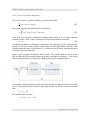
Figure 6 gives a typical closed-loop control system. The Q and R matrices are set by the
user and that effects the optimal control gain that is generated to minimize J. The closedloop control performance is effected by changing the Q and R weighing matrices.
Figure 6 Closed-Loop Control System
For example, assume the plant model in [19] represents the movement of a linear cart where
state x1 is the position of the cart and x2 is the speed of the cart. For the reference command
state
xd = [ xd, 1, 0 ]
T
the controller takes the form
u = −kp ( x1 − xd, 1 ) − kv x2
Revision: 01 Page: 25
QNET Gantry Laboratory Manual
where the optimal control gain is
K = [ kp, kv ]
.
This is a PV controller with a proportional gain, kp, and a velocity gain, kv that makes the
cart track a commanded position xd,1(t). Table 11 lists the resulting PV gains generated
using the linear quadratic regular method from different weighing matrices.
Case
1
2
3
1
Q = ⎡⎢⎢
⎣0
5
Q = ⎡⎢⎢
⎣0
1
Q = ⎡⎢⎢
⎣0
Q
0⎤
⎥
1⎥⎦
R
K
R=1
K = [ 1.0000, 1.7321 ]
0⎤
⎥
1⎥⎦
R=1
K = [ 2.2361, 2.3393 ]
0⎤
⎥
5⎥⎦
R=1
K = [ 1.0000, 2.6458 ]
Table 11 Resulting LQR gain from different Q and R matrices
The first case may not have resulted in overall suitable tracking, therefore some weight is
placed on the top-left Q matrix element to place emphasis on the proportional control. This
translates to the LQR algorithm working harder on the x12 term to minimize the J cost
function and it generates a larger kp. However, as shown in Table 11, it was necessary to
increase both kp and kv gains to minimize J due to the inherent system dynamics. Perhaps
the kp gain generated in case 1 provided suitable tracking performance except that the
closed-loop response tends to overshoot too much. The overshoot can be dampened by
augmenting the velocity gain. The bottom-right element of Q is increased in case 3 and
results in a larger kv while maintaining the proportional gain steady.
The R weighing matrix is kept at 1 in all cases for comparison purposes. If R is decreased
this forces the control input u to work harder to minimize J, resulting in an overall higher
gain K.
4.4.3. Gantry Control Specifications
The whole point of developing a linear model of the gantry and calculating its various
parameters are so a gain can be generated that will control the gantry. In the end, it all
comes down to tuning the Q weighing matrix, as in the Section 4.4.2, such that a closed-
Revision: 01 Page: 26
QNET Gantry Laboratory Manual
loop response meets certain requirements. The LQR control design specifications are:
(1) Tracking: θ(t) track commanded angle θd(t) with tp<1.2 s and ts < 2.3 s.
(2) Dampening: |α(t)| < 7.5 and ts < 6 s
(3) Control input limit: Vm < 5 V
where tp is the peak time, ts is time for the 1% settling time, and Vm is the motor
input voltage.
These are similar specifications to a crane moving boxes within a factory floor. The
pendulum link may be thought of as the actual crane and the weight at the end represents
the box to be moved. The arm is the device moving the crane. Thus the arm must track a
given commanded position and do that with reasonable speed (for productivity purposes),
thus low peak time. This task must be performed accurately as well to place the box in the
correct location, thus low steady-state error with a reasonable settling time is a requirement.
However, the arm control alone does not guarantee that the box will be delivered to the
target location accurately, or safely, because the crane holding the box (i.e. the pendulum
and the pendulum weight at the end) is prone to large swings. The swings are minimized by
having a control that takes into account the position and speed of the crane's angle. Lastly,
the controller must meet the performance specifications within the voltage capability of the
DC motor.
5. In-Lab Session
5.1. System Hardware Configuration
This in-lab session is performed using the NI-ELVIS system equipped with a QNETROTPEN board and the Quanser Virtual Instrument (VI) controller file
QNET_ROTPEN_Lab_03_Gantry_Control.vi. Please refer to Reference [2] for the setup
and wiring information required to carry out the present control laboratory. Reference [2]
also provides the specifications and a description of the main components composing your
system.
Before beginning the lab session, ensure the system is configured as follows:
QNET Rotary Pendulum Control Trainer module is connected to the ELVIS.
ELVIS Communication Switch is set to BYPASS.
DC power supply is connected to the QNET Rotary Pendulum Control Trainer
module.
The 4 LEDs +B, +15V, -15V, +5V on the QNET module should be ON.
Revision: 01 Page: 27
QNET Gantry Laboratory Manual
5.2. Experimental Procedure
Please follow the steps described below:
Step 1. Read through Section 5.1 and go through the setup guide in Reference [2].
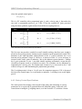
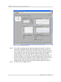
Step 2. Run the VI controller QNET_ROTPEN_Lab_03_Gantry_Control.vi shown in
Figure 7.
Figure 7 QNET-ROTPEN VI
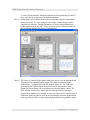
Step 3. Select the the Control Design tab shown in Figure 8.
Revision: 01 Page: 28
QNET Gantry Laboratory Manual
Figure 8 Open-Loop Stability Analysis
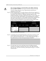
Step 4. Update the model parameter values in the top-right corner with the pendulum
center of mass, lp, and the pendulum's inertia, Jp, that both calculated in Exercise
4.3 and entered in Table 10. The linear-state space model matrices A and B, on
the top-right corner of the front panel, as well as the open-loop poles, situated
directly below the state matrices, are automatically updated as the parameters
are changed. Vary the inertia of the pendulum, Jp, as indicated and observe the
changes in the locations of the poles.
Jp (kg.m2)
Poles
1
2
3
4
1.00E-004
-0.18+9.47i -0.18-9.47i
-0.57+0.00i 0.00+0.00i
2.00E-004
-0.15+8.57i -0.15-8.57i
-0.57+0.00i 0.00+0.00i
Revision: 01 Page: 29
QNET Gantry Laboratory Manual
Jp (kg.m2)
Poles
1
2
3
4
4.00E-004
-0.11+7.34i -0.11-7.34i
-0.57+0.00i 0.00+0.00i
8.00E-004
-0.07+5.93i -0.07-5.93i
-0.57+0.00i 0.00+0.00i
Step 5. How does increasing the inertia effect the open-loop poles and the stability of
the gantry? Shortly explain how a pendulum with more inertia results in this
trend.
Solution:
As the inertia of the pendulum is increased the imaginary part of the poles
and the real part of the poles decrease. The poles are therefore drifting
towards the real axis but also becoming less stable as they slide closer to the
imaginary axis.
The imaginary component decreases because a pendulum with more inertia
tends to keep moving and have oscillations at a lower frequency. The
oscillations of a pendulum with higher inertia is at a lower frequency but
those oscillations tend to have a larger amplitude because they attain higher
pivot accelerations. These larger amplitudes are a sign of being less bound.
Step 6. Under the open-loop poles in this VI it indicates the stability of the gantry
system as being marginally stable, as shown in Figure 8. According to the
poles, why is the open-loop gantry considered to be marginally stable and not
stable?
Solution:
The open-loop poles are not all located in the left-hand plane, there is always
one pole sitting at the origin. The open-loop gantry is therefore not
considered to be stable.
Step 7. As depicted in Figure 8, the controllability matrix is shown in the bottom-right
area of the front panel along with an LED indicating whether the system is
controllable or not. The rank test of the controllability matrix verifies that the
gantry is a controllable system, that is
rank[B AB A2B A3B] = 4
is equal to the number of states in the system. Since the system is controllable, a
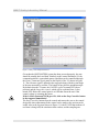
controller can be developed. Click on the Closed-Loop System tab shown in
Figure 9 to begin the LQR control design.
Revision: 01 Page: 30
QNET Gantry Laboratory Manual
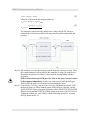
Figure 9 LQR Control Design Front Panel
Step 8. The Q and R weighing matrices and the resulting control gain K is in the topleft corner of the panel. Directly below the LQR Control Design section is a
pole-zero plot that shows the locations of the closed-loop poles. The numerical
value of the poles are given below the plot along with the resulting stability of
the closed-loop system. The step response of the arm angle, θ(t), and the
pendulum angle, α(t), are plotted in the two graphs on the right side of the VI,
as shown in Figure 9. The rise time, peak time, settling time, and overshoot of
the arm response and the settling time of the pendulum angle response is given.
Further, the start time, duration, and final time of these responses can be
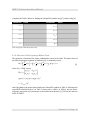
changed in the Time Info section located at the bottom-right corner of the VI.
Step 9. For the Q and R weighing matrices
Revision: 01 Page: 31
QNET Gantry Laboratory Manual
⎡⎢ q1
⎢0
⎢⎢
Q = ⎢⎢
⎢⎢ 0
⎢0
⎢
⎣
R=1
0
0
q2
0
0
q3
0
0
0⎤
⎥
0 ⎥⎥
⎥⎥
0 ⎥⎥
⎥
q4⎥⎥
⎦
vary the q1, q2, q3, and q4 elements as specified in Table 12 and enter the
obtained time-domain characteristics in the same table. Referring to the
feedback loop in Figure 6, for the LQR gain
K = [ kp, θ, kp, α , kv, θ, kv, α ]
T
[25]
the control input u(t) that enters the DC motor input voltage is
Vm = kp, θ ( x1 − x1, d ) + kp, α x2 + kv, θ x3 + kv, α x4
[26]
where kp,θ is the proportional gain acting on the arm, kp,α is the proportional gain
of the pendulum angle, kv,θ is the velocity gain of the arm, and kv,α is the
velocity gain of the pendulum. Observe the effects that changing the weighing
matrix Q has on the gain K generated and, hence, how that effects the properties
of the closed-loop step response. See Section 4.4.2 for some guidance on tuning
an LQR controller.
θ
Q
tp (s)
α
q1
q2
q3
q4
ts (s)
OS%
ts (s)
5
0
0
0
1.12
7.29
8.86
23.76
5
0
0
5
1.15
2.93
14.02
5.5
5
0
0.5
5
1.23
2.12
3.38
5.54
11
0
0.8
12
1.2
2.16
5.83
5.36
Table 12 LQR Control Design
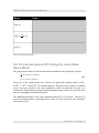
Step 10. Re-stating the LQR specifications given in Section 4.4.3:
(1) Tracking: θ(t) track commanded angle θd(t) with tp<1.2 s and ts < 2.3 s.
(2) Dampening: |α(t)| < 7.5 and ts < 6 s
(3) Control input limit: Vm < 5 V
where tp is the peak time, ts is time for the 1% settling time, and Vm is the motor
input voltage. Find the q1, q2, q3, and q4 elements that results in specifications
Revision: 01 Page: 32
QNET Gantry Laboratory Manual
(1) and (2) being satisfied. When the response meets requiremetns (1) and (2)
move on to the next step to test the third specification.
Step 11. Although the specifications are met, there is guarantee that the control input,
the motor voltage Vm, is not going out of its range. Control design is often
limited by the actuator. Through simulation, it can be checked whether the
control signal is going beyond 5 Volts. Select the Control Simulation tab and
the front panel illustrated in Figure 10 should load.
Figure 10 Closed-Loop Gantry Simulation VI
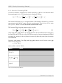
Step 12. The Gantry Command Signal panel enables the user to vary the amplitude and
frequency of the smoothed square signal. The position command signal,
denoted θd(t), is plotted on the top-left graph in Figure 10. The LQR gain
generated by the LQR design in the previous step is shown below in the
bottom-left corner along with a switch that activates the gantry control. The
OFF or down position only enables the arm tracking but does nothing to
dampen the pendulum. For example, as shown in Figure 10 the closed-loop θ(t)
simulation on the top-right is more-or-less tracking the reference signal shown
in the top-left plot. However, the bottom-right plot shows the pendulum angle
Revision: 01 Page: 33
QNET Gantry Laboratory Manual
α(t) and it is swinging back and forth over ±10°. When the switch is activated
the gantry control implemented previously is simulated and that dampens the
swinging of the pendulum. Lastly, the DC motor input voltage is simulated on
the bottom-left scope. Experiment by switching the GANTRY Control switch
ON and OFF and changing the reference signal.
Step 13. For an angle command of 120 degrees at 0.1 Hertz, verify that the gantry
control signal Vm does not exceed ±5V specification. Make sure the GANTRY
control switch is ON when observing control signal. If Vm satisfies requirement
(3) click on the Acquire Data button to return to the Control Design VI and go
to the next step. If Vm does not meet specification (3) and went over the limit,
click on the Acquire Data button, which bring you back to the control design
VI, and tune your controller such that gain K is decreased. Return to the
simulation, by clicking on the Control Simulation tab, with the re-tuned
controller and confirm that the control input does not exceed ±5V.
Step 14. At this point a control has been found that satisfies specifications (1), (2), and
(3). Enter Q matrix elements q1, q2, q3, and q4 in the last row of Table 12 along
with the resulting peak time, settling time, and overshoot for θ as well as the
settling time for α. The control is now ready to be implemented on the actual
gantry device. Click on the Control Implementation tab and the VI shown in
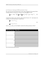
Figure 11 should open.
Revision: 01 Page: 34
QNET Gantry Laboratory Manual
Figure 11 Gantry Control Implementation VI
Given that the QNET-ROTPEN system has been powered properly, the arm
should be rotating back and forth. Similarly to the control simulation VI, the
command position is a smoothed square signal that can be controlled through
the Gantry Command Signal panel on the top-left of the VI, shown in Figure
11. The reference signal is plotted in the top graph along with the actual angle
of the arm measured by encoder. The bottom scope plots the pendulum angle.
By default when the VI opens, the GANTRY control is turned OFF (down
position) and the Integrator control, which will be explained later, is also
turned OFF. Below the control gains is an LED that warns the user if the
control voltage is saturating the motor.
If the Is Motor Saturated? LED goes ON, click on the Stop Controller button
in the top panel immediately!
The Stop Controller button stops the control and returns the user to the control
design tab where adjustments to the control can be made or the session can be
ended. Also in the top panel shown in Figure 11 is the RT LED that indicates if
real-time is being held, the simulation time readout, and the sampling rate.
Revision: 01 Page: 35
QNET Gantry Laboratory Manual
Slow down the sampling rate if the RT LED is either RED or flickering
between GREEN and RED. Also, stop the control by clicking on the Stop
Controller button return to the Control Implementation tab for the new
sampling rate to take effect.
Step 15. Set the command angle to 120° and the frequency of the reference signal to 0.1
Hz. The pendulum should be swinging in excess of ±10° as seen on the α(t) plot
and visually on the actual device. Keeping in mind the behaviour of the
pendulum when there is no gantry control, set the Gantry Control switch to ON
to activate the full LQR control designed. This should dampen the pendulum
angle and meet specification (2). The pendulum should remain suspended in the
downward vertical position as the arm swivels to track the commanded
position. Thus the arm should more-or-less track the reference signal and the
pendulum should remain about its suspended 0 degree position.
Activated
Pendulum
Arm Tracking
Controller
Gantry
Ki
Control (V/rad/s)
Dampening
tp (s)
ts (s)
ess (deg)
max |α |
(deg)
ts (s)
OFF
0
1.7
1.8
25
N/A
19.5
ON
0
1.3
2.2
25
3.3
10
ON
1.4
1.3
2.7
0
N/A
12
Table 13 Closed-loop time response characteristics
Step 16. As probably noticed, the implemented gantry control does not perform as well
as the simulated control. Namely, there is a large steady-state error when θ
track θd and small oscillations about α = 0° are not being dampened. Why are
these phenomenon seen only when implementing the controller?
Solution:
The model developed does not take the friction acting on the θ and α pivots.
More specifically, the Coulomb friction or stiction at the arm pivot prevents
small voltages from the controller to move the arm and compensate for the
slight movements of the pendulum.
Step 17. The steady-state error can be significantly reduced by adding an integral
component. Thus adding an integrator with gain Ki to the LQR control loop
shown in Figure 6 gives the closed-loop system depicted in Figure 12. Thus the
control becomes
Revision: 01 Page: 36
QNET Gantry Laboratory Manual
Vm( t ) = ulqr( t ) + uint( t )
[27]
where the LQR control and integral control are
ulqr( t ) = −K ( x( t ) − xd( t ) )
and
uint( t ) = −
Ki ( x1( t ) − x1, d( t ) )
[27]
s
.
The integrator control basically pumps more voltage into the DC motor to
eliminate the offset between the actual arm position and the commanded arm
position.
Figure 12 LQR+I Closed-Loop System
Step 18. The task now is to tune the integrator gain Ki until θ(t) converges to θd(t). Thus
the control parameter will be tuned as the controller is being ran on the device.
Record the Ki gain used in Table 13 along with the corresponding response
properties.
If the Is Motor Saturated? LED goes ON, click on the Stop Controller button
in the top panel immediately! In this case, reduce the Ki until the LED goes
OFF because the gain is set too high and is saturating the motor.
Step 19. Click on Stop Controller and the Control Design tab should be selected. If all
the data necessary to fill the shaded regions of the tables is collected, end the
QNET-ROTPEN Gantry laboratory by turning off the PROTOTYPING POWER
BOARD switch and the SYSTEM POWER switch at the back of the ELVIS unit.
Unplug the module AC cord. Finally, end the laboratory session by selecting
the Stop button on the VI.
Revision: 01 Page: 37