Download SharkPlotter Manual - Sirius Cybernetics LLC

SharkPlotter Manual
Introduction
"SharkPlotter" is a companion program for JDSPorsche's "SharkTuner" for the Porsche
928. The purpose of SharkPlotter is to assist with the review of data that was logged from
SharkTuner and to provide some tools for further optimization of fuel and ignition tuning.
It provides plots of AFR vs. MAF load and RPM for the LH processor, plots of knock
events vs. load and RPM for the EZK, and the ability to manually or automatically adjust
the LH and EZK maps for the best "fit" with the data and review the results.
The simplest use of Sharkplotter is to go for a drive and log data with the SharkTuner,
then take the data home and review it. And then, if needed, make adjustments to the maps
over the conditions that were encountered. Changes can either be made manually (in the
same fashion as adjusting a SharkTuner map) with the effects shown on the plot, or
automatically optimized against a table of desired AFR values. Knock events can also be
displayed and related to fuel status, and ignition timing can be retarded as necessary
either manually or automatically.
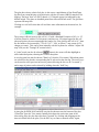
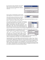
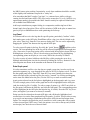
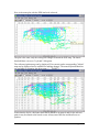
The basic SharkPlotter window is shown below. The main window area is a color-coded
AFR plot on a grid that matches the LH correction map, engine load (SharkTuner's "MAF
signal/absolute") vs. RPM. Air/fuel ratio is shown as color, from yellow as too rich
through green and blue (stoich) to purple and red as too lean. The plot is scaled to actual
MAF and RPM values, with each grid-square represents a LH adjustment "cell" (hence
the irregular grid).
SharkPlotter ver 0.9
Copyright © 2009 Jim Corenman
revised 2009-09-07
The plot above shows a basic fuel plot, in this case a consolidation of four SharkTuner
log files from casual driving on local twisties with the O2 sensor (NBO2) turned off for
logging. The large "dots" are WOT throttle (>2/3 throttle approx) as indicated by the
throttle switch. Grey dots are disabled points from idle-switch fuel cutoff. The grid lines
represent LH map cells.
Clicking on a cell will select that cell and show more information in the status-bar, for
example:
The average A/R fuel ratio for this cell is 14.2 with a Standard Deviation of 0.5 (i.e. 2/3
of all the points lie within 0.5 of the mean), and there are 162 points logged in this cell
(the more points, the more meaningful the results). So if the goal for this cell is 14.7 then
the fuel needs to be increased by 3.5% (0.5/14.7 * 100), or about 17 map counts (0.2%
change per count). This can be done manually with the keyboard or with the "Adjust LH
map" tool (see the "Tuning LH" section below).
A "point" mode can also be selected (
button), the cursor will then highlight or
select individual points, showing the AFR for that point.
A text-log panel can also be shown ("Data Log" from the View menu). When data points
are selected on the plot the corresponding line is selected on the data log. The arrow keys
can be used to select previous/successive points (allowing the drive to be "recreated"),
and a range of points can be selected by holding down the "shift" key.
A time-plot for RPM, MAF and AFR can also be shown across the bottom of the plot
("Data Plot" from the View menu). Initially this shows the entire time-span of the
selected log files, the plot above has been "zoomed" by clicking and dragging on the
time-axis labels below the plot. (Use the ESC key to return to normal zoom). Again,
pg. 2/25
points selected on the fuel plot are highlighted on the data time-plot (and log panel if
visible), and vice-versa. The stats are shown at the bottom of the window. See "Data
Graphs" for more details.
If Knock-retard values are logged then the plot will also show knock-events, there are a
few high-load/low-RPM knocks in the plot above, some around 1900 RPM and one at
2800. (This is a stock S4. Most knocks happen in the 3300-4000 RPM max-torque area
but the S4 ignition is pretty retarded there—this is a horsepower opportunity with careful
tuning).
"Mousing-over" a knock event will display information about that knock:
SharkPlotter also provides separate windows for managing LH and EZK maps (similar to
SharkTuner's map windows), and a Project window for managing project files.
SharkPlotter assumes that all SharkTuner log files are stored in one place, with a separate
folder for each "Project" (i.e. for each car), and separate folders under that for each
"Session" (a set of log "run" files recorded with the same maps). This organization does
not have to be used—SharkPlotter can utilize log files stored anywhere—but using the
Project window makes it easier to keep track of things.
The next section will do a quick walk-through for a car in a reasonable state of tune (a
relatively stock S4). Subsequent sections will describe each program window and
function in detail, followed by some more detailed technical information which may be of
interest.
A caveat: Remember that SharkPlotter, and SharkTuner, are tools. Like
many tools they can, if misused, cause damage. The hazards of some
tools, like hammers, are obvious. That is not the case with software
programs, so please take the time to read this manual and the SharkTuner
manual carefully before taking on a tuning project. If you are not sure how
to proceed then ask, see the support information at the end of this manual.
The knowledgeable folks on Rennlist may also be able to offer help and
advice, but exercise a bit of caution with an public forum.
Happy tuning!!
pg. 3/25
Quickstart Guide
In order to use the SharkPlotter software, data must first be logged from the SharkTuner.
This can be done on the road or with a series of dyno runs. Basic fuel tuning can easily be
done on the road, while ignition tuning for max horsepower is done most easily with a
series of carefully-planned dyno runs.
For cars originally fitted with catalysts and an O2 sensor, the LH operates in a "closedloop" mode for lighter engine loads, automatically adjusting AFR as needed. Tuning
should be done in open-loop mode, without these automatic adjustments. The simplest
way to force open-loop operation for cars equipped with O2-sensors is to disconnect the
O2 signal lead from the LH. This can be done by inserting a "test" switch into the black
wire from the NBO2 sensor (i.e. on the sensor side of the NBO2 disconnect under the CE
panel). A "pigtail" cable is available from JDSPorsche to accomplish this (along with
providing convenient connections to a WBO2 sensor). Open the switch to log data for
tuning, close it for normal operation. Also be sure to disable and reset "O2-adaptation" on
the Fuel-parameters page.
To start logging, start the SharkTuner software and download from PEM's (File menu).
To log open-loop (without using the NBO2 sensor) either open the "test switch" (above)
or select the "Fuel parameters" tab and select "Force non-cat mode" (center of window),
and verify that "CO Pot in non-cat mode" is disabled (lower-left).
Next, save a copy of the base fuel map. Do this by selecting SharkTuner's "Fuel maps"
page, select the appropriate base-map ("no-cat" if the car does not have an O2 sensor or
the "Force no-cat" option was selected, "cat" otherwise). Select all map cells, this can be
most easily done by clicking the upper-left gray border cell (not the upper-left table cell),
the entire map is then selected. Then press the Ctrl-C keys to copy these cells to the
Windows clipboard. Now start SharkPlotter and click the "Open project" button. For
first-time use click "Browse" and select the SharkTuner logs folder (create a new one if
needed), then click "New Project" to create a new project-folder if needed, then click the
"New Session" button. The default folder-name is the date (in year-month-day format to
assist with sorting), add any desired description. Then click the "Paste" button to the right
of the "Fuel map" box, this will create a file and save the copied fuel map.
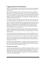
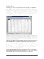
Then select the "Data Logging" tab and select the desired parameters. Select "RPM",
"MAF signal (absolute)" "A/F ratio" and "O2 sensor adj" from the "Fuel Variables" box,
and "Knock retard" and "Load" signals from the "Ignition variables" box.
pg. 4/25
A logging rate of 10 samples/sec is generally adequate. Remember that Sharktuner log
runs are limited to 5000 samples per run (about 8 minutes at 10/sec), and a faster sample
rate will require restarting the log more frequently.
The figure above shows the suggested parameters for logging if PEM's are fitted to both
LH and EZK. Note that "Throttle position" was selected from the LH side, this is because
the WOT switch is often disconnected from the EZK in order to disable the separate
WOT ignition map.
Then go for a drive. The goal is simply to collect data over a wide range of driving
conditions, and a co-pilot is handy to start and restart the SharkTuner's data logger as
needed. When a logging run gets near 5000 lines (i.e. close to 500 seconds in the first
column), click the "stop/start" button twice to stop the log and start the next. (If it reaches
5000 lines and stops, then just click the button once to restart). When finished with
logging then save each run by clicking the "save run" button, saving the files into the
session folder that you created above. Use the normal "Run 1" file names, an additional
notation can be added to the file-name if desired but retain the original "Run 1" so that
SharkPlotter will recognize the log files and show them chronologically.
When you are done, open SharkPlotter and click the Open-project button (or "Open
Project" on the File menu) and most recent project/session files will open. Click "OK".
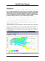
SharkPlotter should be showing the logged data as an air/fuel plot versus RPM and MAF
signal. Ideally the light-load areas (upper half of the plot) are stoichiometric or nearly so,
and the high-load areas (lower half) are a bit richer (e.g. 13.2) for optimum power.
The color is the first indication of fuel status, a stoichiometric mixture is indicated by a
blue-green color. Green or green-yellow is slightly rich, desirable for max power in openloop mode (higher loads or WOT), and yellow is overly rich, 12:1 or richer. Purple and
red indicate overly-lean mixtures and are a cause for concern especially in the higher-
pg. 5/25
load cells. (This plot shows a typical S4, pre-SharkTuning: some lean spots, and overly
rich in the lower-right high-load/higher RPM area of the plot).
Now open the Fuel-Maps from the Window menu. The first "Reference" tab is the base
fuel map that you copied and saved. The next tab is for adjustments (more in a moment),
and the third tab is the resulting "Updated" map. Click on the last tab—this is the "Target
AFR" map, which SharkPlotter will use to adjust the fuel map. Verify that this represents
the desired AFR for the various map areas, select cells and use the "+" and "-" keys to
adjust. The light-load areas should be stoichiometric (14.7) or slightly rich, moderate load
should trend towards richer, and high-load areas should be 13.2 for best horsepower, or
richer as desired for protection with boosted engines.
Now go back to the main window. To have SharkPlotter automatically adjust the fuel
map to the target AFR's, select "Adjust Fuel Map" from the Tools menu. SharkPlotter
will scan the fuel map and adjust each cell as close to the Target AFR as possible,
iterating a few times in order to do the interpolation between cells in the same way that
the LH does. When it finishes (a few seconds), open the Fuel Maps window again, select
the "Updated" tab, check for any goofy points and click the "Copy" button. This places a
copy of the updated map in the clipboard, where it can be transferred back to
SharkTuner's base fuel map (click the upper-left cell and type Ctrl-V to paste).
If there are excessive knock events (large "X" symbols) then the ignition map can be
similarly adjusted with the "Adjust Ignition map" selection from the Tools menu. Once
complete select "Ignition maps" from the Window menu, check the results on the
"Updated" tab, and copy this to the SharkTuner's EZP maps page as above.
The following sections will cover these topics in more detail, starting with project
management.
pg. 6/25
Project Management
Effective use of the SharkPlotter depends on keeping log files and maps organized. There
are many ways to do this, but arguably the simplest— and the and the and the method
supported by SharkPlotter— is to create a folder for log (and map) files, under that create
folders for each project (i.e. different cars, or different developments for one car), and
under that create folders for each tuning session for a series of logs created with the same
maps, and a copy of those maps. After each session the logs can be reviewed with
SharkPlotter, adjustments made as needed and then copied back to the SharkTuner, and a
new session begin.
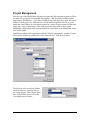
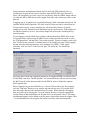
SharkPlotter supports this organization with the "Project Management" window. To start
a new project or open an existing one, select "Open Project" from the File menu.
The first box is the overall log folders,
and below that is a selection box for
the current project. This is a pull-down
box, click the little arrow to see a list
of available project folders.
pg. 7/25
To create a new project click the "New Project"
button and enter a name for the new project.
(The name must be a legal filename, avoid the
characters / \ : * ? " < > | ).
Once a project is selected then a session can be
selected from the "Current Session" box. This is
also a pull-down box, click the arrow and select
an existing session folder from the list. And a
new session can be created with the "New Session" button in the same fashion as a new
project, creating a new, empty session folder.
If an existing session folder is opened then all text files in
that folder will be listed in the "Log Files" box. Files that
appear to be log files (i.e. have "Run" as part of the
filename, and contain the minimum required data—Time,
RPM, MAF, AFR—will be checked and displayed in the
main AFR plot. Other files can be selected (checked), but
if they are not the correct format then error messages will appear.
If fuel and ignition maps are found then these are also listed, and loaded for the current
plot. Initial map files are recognized if they contain
"initial", "base" or "starting" as part of the file name, and
either "fuel" or "LH" for fuel maps and "Ign" or "EZK"
for ignition maps. Alternately a fuel or ignition map can
be copied from the SharkTuner's Fuel-maps or Ignitionmaps tab and pasted into SharkPlotter by clicking the appropriate "Paste" button. This
creates an appropriately-named file, saves the map and opens the file.
Organizing project and session folders in this hierarchy under a common "logs" folder is
convenient and is supported by SharkPlotter's Project-Manager window, but is certainly
not required. Log files and maps can be saved anywhere in any desired arrangement, and
opened with the "Open Log File" and "Load map file" selections under the File menu.
These menu selections display the standard Windows file-open dialog allowing selection
of any folder. Multiple log files can be opened together by holding down the Shift or Ctrl
keys while selecting files, in the usual Windows fashion.
pg. 8/25
Logging data from the SharkTuner
In order to use the SharkPlotter software, data must first be logged from the SharkTuner.
This has been discussed above in the "Quick Start" section, this section will add some
additional detail.
One issue for fuel tuning is that the LH, when fitted with an O2 sensor, automatically
adjusts AFR with a closed-loop control loop in "cruise" mode (i.e. for lighter engine
loads). This is necessary for the use of catalytic converters which require an average AFR
very close to stoichiometric to operate properly. The LH achieves this with closed-loop
correction based on O2-sensor readings—both a short-term "O2-adjust" correction in
addition to a longer-term "O2-adaptation" correction which is stored the LH memory. See
"LH Basics" for more information.
The O2-adjust correction can be logged by the SharkTuner and can be used as the basis
for adjusting the LH map in the lighter-load areas. (This won't work for the higher-load
map areas and WOT, because the LH will be in open-loop mode).. It is more accurate,
however, to disable the LH's closed-loop mode and operate it open-loop (with fuel based
strictly on map values), and then use the logged WBO2 values as the basis for map
adjustments. The SharkTuner's "Autotune" function does this by forcing open-loop
operation using the normal "cat" maps. This mode cannot be selected for the logging
function, but there are two other alternatives.
As discussed, open-loop operation can easily be selected by fitting a "tune" switch to
disconnect the NBO2 sensor signal lead (the black wire on the sensor side of the NBO2
disconnect under the CE panel). Open the switch to log data for tuning and close it for
normal operation.
The other method of selecting open-loop operation is to select the SharkTuner's "Force
no-cat operation" option on the Fuel-parameter page. This will switch the LH to openloop operation, but will also select the "no-cat" maps. So it is also necessary to copy the
contents of the "cat" base map to the "no-cat" map, so that the same base fueling will be
used as for normal operation. Also be sure to disable the CO-pot unless one is fitted,
otherwise the LH will read the open-circuit CO-Pot connection as a maximum pot value
resulting in excessive fuel.
And always be sure to disable and reset "O2-adaptation" on the Fuel-parameters page, to
prevent the LH from adjusting fuel values from previously-stored adaptation values.
These values are reset when the power is interrupted to the LH (i.e. battery disconnected
for a period of time) but do the disable/reset to be sure.
Selection of log variables
For tuning fuel, the required parameters are "RPM", "MAF signal (absolute)", and "A/F
ratio" (from the WBO2 sensor). To check closed-loop fueling (or to verify that open-loop
operation was correctly selected) "O2-adjust" should be added to this list, as well as
"Throttle position" to log the idle and WOT switches. For the EZK, the variables "Knock
retard" and "Load" signals should also be logged in order to monitor knocks and make
any needed timing-map adjustments,.
pg. 9/25
Some parameters are duplicated on both the LH (fuel) and EZK (ignition) side, e.g.
coolant temp. In general it is better to log these from the EZK side as the data-rate is
faster. The exception is A/F ratio, since it is read directly from the WBO2 sensor and not
via either the KH or EZK then it can be logged from either side without any effect on the
data rate.
A logging rate of 10 samples/sec is generally adequate. With a minimum selection of LH
variables (RPM, MAF-signal/abs, A/F ratio) a rate of 20/second can be selected but the
LH can't quite keep up, so the actual data rate will somewhere between 10 and 20
samples per second. Remember that Sharktuner log runs are limited to 5000 samples per
run (about 8 minutes at 10/sec), and a faster sample rate will require restarting the log
more frequently.
To start logging, start the SharkTuner software and download from PEM's (File menu).
To log open-loop (without using the NBO2 sensor) either open the test-switch or select
the "Fuel parameters" tab and select "Force non-cat mode" (center of window), and verify
that "CO Pot in non-cat mode" is disabled (lower-left). Finally select the "Data Logging"
tab and select the desired parameters. As a minimum, log "RPM", "MAF signal
(absolute)" and "A/F ratio" on the LH side, plus "O2 sensor adj" for closed-loop
operation.
The figure above shows the suggested parameters for logging if PEM's are fitted to both
LH and EZK. Note that "Throttle position" was selected from the LH side, this is because
the WOT switch is often disconnected from the EZK in order to disable the separate
WOT ignition map.
When a logging run gets near 5000 lines (i.e. close to 500 seconds in the first column),
click the "stop/start" button twice to stop the log and start the next. (If it reaches 5000
lines and stops, then just click the button once to restart). When finished with logging
then save each run by clicking the "save run" button. Be sure to select the appropriate
session-folder so that SharkPlotter can find the files. Use the normal "Run 1" file names,
an additional notation can be added to the file-name if desired but retain the original "Run
1" so that SharkPlotter will recognize the log files and show them chronologically.
pg. 10/25
Description of SharkPlotter Windows
Main Fuel-plot window
The main SharkPlotter window is an AFR (Air/Fuel Ratio) plot, showing individual
logged data points as colored dots plotted against RPM on the horizontal axis and engine
load (MAF signal/absolute) on the vertical axis. This corresponds to the LH's base
correction map and allows easy visualization of which cells need adjustment.
The color-coding is shown as an AFR scale, a colored bar which shows which colors
correspond to what AFR. Red indicates too lean, blue/green is stoich, slightly rich is
green and excessively rich is yellow. This scale can be moved as desired (click and drag)
and disabled with the View menu.
There are two buttons to select the mouse mode: Cells( ), or Points ( ). In "Cells"
mode (the initial selection) moving the mouse over the plot will "highlight" the cell under
the cursor with an outline box, and the average AFR for the points in that cell will be
shown in a "hint" that follows the cursor, along with the deviation and number of points.
If the plot is clicked then the highlighted cell becomes "selected", shown by outlining the
cell and fading the non-selected cells. More than one cell can be selected by holding
down the "Ctrl" key while clicking on additional cells. The status-bar then shows the
statistics for the selected cell (or cells): the average (mean) AFR, the standard deviation,
and the number of points.
Point mode works similarly except individual data points are highlighted by being
brought to the top with a border, and the AFR for that point is shown. If the plot is
clicked then that point becomes selected and the AFR is shown in the status-bar, along
with any knock information.
Copying maps to/from SharkTuner:
To update the LH base fuel map in the SharkTuner, the map must first be copied from
SharkTuner to SharkPlotter. Select SharkTuner's fuel-maps page, make sure the
appropriate base-fuel map is selected and then select all of the map cells. This can be
most easily done by clicking the upper-left gray border cell (not the upper-left table cell),
the entire map is then selected. Then press the Ctrl-C keys to copy these cells to the
Windows clipboard. Then either open SharkPlotter's Project window and use the fuelmap "Paste" button, or open the Fuel-maps page, Reference Map, and click "Paste Map"
(or press the Ctrl-P keys).
Some things to note
First, for cars with NBO2 sensors running in closed-loop ("Cat") mode, remember that
under most conditions the LH processor uses the NBO2 sensor to drive the AFR back to
stoich, AFR=14.7 (See "LH Basics" below). So changes to the LH base fuel map really
make no difference as long as the LH is running closed-loop, other than keeping the AFR
correction "centered". However there are plenty of times that the LH will run open loop:
higher RPM's and load (even without the WOT switch), during warmup, and of course if
pg. 11/25
the NBO2 sensor quits working. In particular, overly-lean conditions should be avoided,
while slightly-rich conditions can provide a "safety net".
Also remember that MAF's tend to "age lean", i.e. estimate lower airflow with age,
causing less fuel and leaner AFR's. The effect can be as much as 3%, or 0.4 AFR (a very
approximate number), beyond this the MAF should certainly be replaced. Rebuilt units
are available from JDSPorsche.
And keep in mind that any engine fueling is a compromise, and having lots of data
doesn't imply lots of precision. There will be variation of AFR in the plot, no matter how
good a job you or SharkPlotter does with optimizing the fuel map.
Log Panel
It is often useful to review the log data for specific points, particularly "outliers" which
don't make sense on the AFR plot. SharkPlotter offers a log view which is linked to the
plot, select "Data Log" from the View menu to display this. The size can be adjusted by
dragging the "splitter" bar between the log and the AFR plot.
To select a specific point in the log, first click the "point" button (
) and then select
a point. The corresponding line in the log will be selected (highlighted) and brought into
view. Successive (or previous) points can be selected with the up/right or down/left keys.
Holding down an arrow key "drives" the selection up and down the log, highlighting
corresponding points on the plot (or vice-versa). While fun, the utility is limited.
To select a series of points, hold down the Shift key while pressing the arrow keys.
Multiple individual points can also be selected by holding the Ctrl key. Statistics for the
selected points are shown in the statusbar at the bottom of the window.
Data Graph panel
It is also sometimes useful to view the data as a graph versus time, in order to pick out
particular segments (e.g. a run through all the gears at WOT) for further review. To show
the data graph panel select "Data Plot" from the View menu. Initially this shows the
entire time-span of the selected log files, but can be "zoomed" by clicking and dragging
on the time-axis labels below the plot. (Use the ESC key to return to normal zoom).
Again, points selected on the fuel plot are highlighted on the data graph, and vice-versa.
To select a single point, click it on the graph and it will be highlighted on the AFR plot
(and also in the log file, if visible). To select a range of points (e.g. a WOT run) click on
the first point, hold down the Shift key and click the final point. The corresponding points
will be highlighted in the AFR plot (and also the log, if visible). Press the ESC key to unselect, and again if you want to un-zoom (if zoomed).
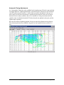
Points can also be selected on the main AFR plot, and will then be highlighted and
scrolled into view on the Data graph and Log file panels, if visible. This provides an easy
way to pick out interesting or anomalous points on the AFR plot and investigate them
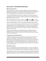
further. For example, the plot below was a casual drive in the countryside with a couple
of short (second-gear) WOT runs. Clearly the mixture is too rich at the top end (S4 with
stock maps), how does the rest of that run look?
pg. 12/25
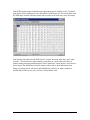
First selecting one of the points near max RPM, that will highlight it both on the graph
and in the log data. Then zoom the graph around that selected point until the beginning
and end of the short WOT run is seen. Then click the beginning on the graph to change
the selection point, then hold down the Shift key and click the end of the run, to select all
of the points. The result is shown below.
This segment started with light throttle at around 1200 RPM (indicated by low MAF load
numbers). Then throttle was slowly rolled on until around 3600 when WOT switch was
tripped (84.60 in the log). The AFR was pretty reasonable up to that point, then became
excessively rich.
The stats for this selection of points are not very meaningful because of the number of
different cells that were traversed, but selecting a smaller range of similar points would
provide good data for adjusting the fueling.
It is also easy to extract this short segment into a separate file—with the interesting points
selected this way, just select Edit menu, Copy (or Ctrl-C from the keyboard). This selects
the lines from the original log for this selection into the Windows clipboard. Open
Notepad document (or some other editor) and paste the selected log except. This allows
pulling individual "strands" out of the plate of spaghetti that results from most over-theroad driving.
pg. 13/25
Fuel Maps Window
Fuel maps can be viewed in a separate window, select "Fuel Maps" from the Window
menu. The Fuel maps window has four tabs, representing four different maps. From the
left the "Reference" map is the base fuel map that was in use when the data was recorded;
the "Adjustments" map represent changes that have been made to this map, either using
SharkPlotter's auto-adjust functions or manually; the "Updated" map is the resulting map
to be copied back to SharkTuner if desired (i.e. Reference map ± Adjustments map); and
the "TargetAFR" map is the desired AFR for each cell, to be used by SharkPlotter's autoadjust function.
Cell values can be copied from or pasted into each page. To copy part of a map, select the
desired cells or click one of the header buttons to select a column or row, then press the
Ctrl-C keys. To copy the entire map either select all of the cells (with the mouse or click
the upper-left border button) and then Ctrl-C keys, or click the "Copy Map" button- this
will copy the entire 16 x 16 map.
Cell values can be pasted into a map from another source (e.g. from a SharkTuner map or
from a saved map opened in Notepad or some other editor). Select and copy the cell
values from the source, and then select the upper-left corner of the destination area and
press the Ctrl-V keys, or click "Paste Map" to paste an entire 16 x 16 map. It is also
possible to paste a row or column (or part of one) into a larger area repeating as needed,
provided that one dimension matches. Or a single value can be pasted into any array of
selected cells. If the shape of the selected destination area is not consistent with the
source area then an error message is displayed.
Changes can be made to individual cells or a selected area of cells on any of the pages.
Select the appropriate cell(s) with the mouse and then use the '+' and '-' keys to increment
or decrement the values by one count, and hold down the Ctrl of Shift keys to
pg. 14/25
increment/decrement by 10 counts. Alternately the "QAWS" keys can be used in the
same manner as for making map adjustments SharkTuner (+1, -1, +10, -10 respectively).
Changing one map updates the others. Changing "Reference" or "Adjustments" maps
(either pasting new values or making changes with the keyboard) also updates the values
shown in the "Updated" map, and changing the "Updated" map updates the values shown
in the "Adjustments" map. This latter function can be used to compare two maps: Paste
the Reference map first, then the Updated map, and the resulting differences will be
shown in the "Adjustments" map.
The "Stay on top" check-box at the bottom of the window will keep the Fuel map
window on top of other windows even if focus is switched away.
Ignition Maps Window
The Ignitions maps window (selected from the Window menu) is similar to the Fuel maps
window, and has three tabs for Reference, Adjustments, and Updated maps for ignition
advance.
Changes can be made by copy/paste or via the keyboard in the same manner as for the
Fuel map, above. The increment/decrement values for the '+' and '-' and "QAWS" keys
are ± 0.4 and ± 3.
pg. 15/25
Fuel tuning
Manual AFR Adjustments
Adjustments can be made to individual cells, either directly on the AFR plot or on the
separate "Fuel maps" window (above). To show map adjustments on the main window,
select "Adjustment map" from the View menu. With the "cell" selection button depressed
(
) select a cell with the mouse, or multiple cells by clicking while holding down the
Ctrl key. Then increment or decrement that cell with the + or – keys (no shift-key
needed) to change by one count, or hold down the Ctrl or Alt keys to change by 10
counts. Alternately use the "QAWS" keys for increments of +1, -1, +10, and -10 counts
respectively (the same key assignments as for SharkTuner map adjustments).
Each increment to the adjustment map here is the same as an increment to the LH
correction map, where ±127 represents a 20% change in fueling— an increment of 5
represents a 0.1 AFR change. The effect of the adjustment for the selected cells will be
shown graphically, and numerically in the status bar.
To make fuel map adjustments on a separate map window, open SharkPlotter's Window
menu and select Fuel Maps. There are four tabs: the "Reference" (starting-point) map, the
"Adjustment" map (for changes entered here), and the "Updated" map—i.e. the reference
map +/- the changes from the "Adjustment" map (and a page for the target AFR for
automatic adjustments).
Automatic LH Map Adjustments
In addition to the manual adjustment described above, SharkPlotter can also make map
adjustments automatically for the best overall fit. This is done by scanning each cell,
computing the difference between the average AFR and the "target" AFR for that cell
(Fuel maps window), and computing an adjustment value. These adjustments are
interpolated to match the LH processor, and smoothed according to a weighting
algorithm so that cells with few points and large errors don't unduly influence the result.
This scan is then repeated up to four times (or until the differences stop getting smaller)
to accommodate interaction between cells as a result of interpolation.
To use the automatic adjustment function, first make sure the appropriate reference map
is loaded. Do this with SharkPlotter's Project manager window, or load a specific map
with the File menu. Then select "Adjust Fuel Map" from the Tools menu.
pg. 16/25
Ignition Tuning
SharkPlotter also offers some tools to help with ignition tuning. If knock-retard is
included with the log files then knock events (an increase in knock-retard for any
cylinder) are displayed on the AFR plot as an "X" through a data point. A light "X"
indicates that the number of cylinders retarded, and the maximum retard, did not exceed
the threshold (3 cyl's and 2 degrees by default). A bold X" indicates that the knock limits
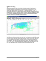
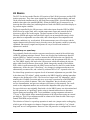
were exceeded, and attention is needed. Here is a plot of mid-range testing (zoomed)
showing a few knocks in the 4000-5000 mid-load area:
The EZK uses a different scale for engine load, the "Load" parameter on the EZK section
of the data log tab (rather than "MAF signal (absolute)" which is used by the LH). If the
EZK Load signal is logged then the AFR plot can also be displayed against the EZK
Load parameter, click the "EZK Plot" button on the toolbar. This changes the vertical
scale to EZK Load, 0-100, and the RPM grid is changed to the RPM limits used by the
EZK. The indicated cells then correspond to the EZK ignition-advance map.
pg. 17/25
Here is the same plot with the EZK-load scale selected:
The plot is the same, only the scaling has changed to match the EZK map. The knock
threshold here was set to 3 cyls and 2.0 deg max.
The reference ignition map can by displayed (View menu), and a corresponding "Adjust"
map can be displayed and is available for making changes. The same keyboard shortcuts
are available for changing the adjust map (+/-, "QAWS").
Notice that the fuel is a bit leaner here than it should be in general, and for the selected
point it may be related to the knock events. Always tune fuel first and then focus on
ignition.
pg. 18/25
Automatic Timing Adjustments
An "Auto update" function is also available for the ignition map. If knock-count and load
are logged then the "Update Ignition Map" selection from the Tools menu will retard the
each cell with excessive knocks, i.e. those which exceed the thresholds. In the case of
max retard over the limit, the advance is retarded by that amount. In the case of knock
detected from too many cylinders, that cell is retarded in 0.4 deg increments until the
cylinder count is within the threshold. The knock marks are updated on the plot, and the
Update map is updated.
Here are the results of updating ignition for the previous plot (adjustment map shown).
The selected point has been retarded 1 deg and now has a predicted max-retard of 1.6
deg.
pg. 19/25
If the EZK ignition map is loaded then the adjustment map is added to a new "Updated"
map which can be copied back to the SharkTuner's EZK maps tab. This can be done with
the EZK-maps window (Window menu) which works in the same way as the fuel maps.
Note that the auto-adjust for the EZK is in the "retard" direction only, there is no "autoadvance". This needs to be done manually, preferably on a dyno where the effect of
ignition timing on torque and horsepower can be measured—more advance is not always
more torque. The SharkTuner's knock-counter will provide a quick indication when
things are getting too far advanced, and SharkPlotter will tell you where attention is
needed and provide an easy way to focus on the problem areas.
pg. 20/25
LH Basics
The ECU for the later-model Porsche 928 consists of the LH fuel processor and the EZK
ignition processor. They share some signals but each functions independently, and both
can be interfaced simultaneously by the SharkTuner using PEM's, special flash-memory
modules that replace the standard pROM's. When the SharkTuner is connected it can
intercept data from either box (assuming both are fitted with PEM's) and either display or
log various engine variables.
Fueling is controlled by the LH processor, which takes inputs from the EZK for RPM,
MAF sensor for engine load, and a coolant temperature sensor and controls the fuel
injectors to deliver fuel to the engine. The basic amount of fuel is determined as a
function of RPM and engine load (the MAF signal) via an internal table (map), which
gets added to an adjustable correction table, and is then adjusted for temperature and
transient conditions (e.g. acceleration). If the measurements were all accurate, and the
engine characteristics precisely known, then the correct fuel quantity could be accurately
calculated. But sensors, engines and injectors all vary a bit and some method of
adjustment is needed.
Closed-loop vs. open-loop
Cars originally fitted with catalytic converters need precise control of the air/fuel ratio
(AFR) for optimum emissions control. These cars are also fitted with narrow-band O2
sensors (NBO2 or "lambda" sensors) to measure the AFR before the cats. Ideally the
AFR will be 14.7 which is the stoichiometric mixture, and the optimum AFR for a 3-way
cat. This NBO2 signal is fed back to the LH processor which then adjusts the injector
pulse-width for any difference from stoich, which changes the amount of fuel and the
AFR, which is again measured by the NBO2 sensor and used by the LH to make further
adjustments—hence the term "closed loop". Any changes in component tolerances are
automatically accounted for, and a relatively constant AFR of 14.7 is passed to the cats.
For closed-loop operation two separate levels of automatic adjustment are provided: First
is the short-term "O2-Adjust", which responds to the NBO2 signal by making immediate
changes to the fueling up to ±20%. The second is a longer-term "O2 Adaptation", which
monitors the O2-adjust correction and saves an average correction for each RPM/MAF
map-cell over a period of minutes. This is the "adaptation" that is referred to in the
service documentation, and gets reset whenever the battery is disconnected. For a welltuned car the adaptation numbers are small and the adaptation table plays little part.
For cars which were not originally fitted with cat's the NBO2 sensor was also omitted and
the LH operates in an "open-loop" mode, using its internal tables alone to determine
injector timing and resulting AFR. To accommodate varying component tolerances a
"CO pot" is fitted which allows manual adjustment of the idle-mixture using an external
gas analyzer. This CO-pot adjustment adds or subtracts fuel from the table values up to
around 2500 RPM (not just at idle).
The selection of closed vs. open-loop operation is made via a jumper on the coding plug,
which is part of the engine wire-harness. Separate tables are provided for "cat" (closedloop) and "no-cat" configurations. However if the LH processor is configured for closed-
pg. 21/25
loop ("cat") operation and the NBO2 signal is missing then it reverts to open-loop. It will
also revert to open-loop operation before the engine is warmed up, or for 20-30 seconds
following a re-start of a warn engine, or for high-load or WOT running.
Note that cars which have had their cats removed are still typically fitted with NBO2
sensors, and operate in a closed-loop "cat" mode. It is the presence of a NBO2 sensor that
allows closed-loop operation, not the cat itself.
WBO2 Sensor Considerations
Something often overlooked is the importance of properly fitting a wideband-O2
(WBO2) sensor. The normal "O2 sensor" (Lambda-sensor) which is fitted standard on
cat-equipped cars is a very narrow-range sensor, with the output going from zero (too
lean) to about 1 volt (too rich) over span of only a few hundredths of air/fuel ratio. This is
perfectly adequate for the LH processor to maintain the average AFR at stoich and keep
the cat's happy, but is not suitable for any serious tuning.
A WBO2 sensor requires a special controller which has a linear output, typically 0 to 5
volts over an AFR range of 9 to 19. The sensor only functions properly at high
temperatures, and WBO2 sensors include a heater and temperature regulator. The WBO2
output provides an accurate measurement of AFR over a wide range, and is required for
using the SharkTuner for anything other than the most basic diagnostics (checking
sensors, etc).
The WBO2 sensor can either be fitted temporarily for testing, or permanently to allow
testing at any time. The optimum arrangement is a bung (threaded adaptor) welded into
the exhaust pipe, downstream of the exhaust manifold or headers and upstream of a
catalytic converter. Tailpipe adaptors are not recommended as the pressure waves from
any decent exhaust system will be pulling in outside air and diluting the exhaust gases.
Ideally the WBO2 sensor should be located at a point where gases from all with cylinders
are mixed, but assuming that the injectors are all functioning properly and reasonably
well matched then sampling one side is fine. A typical "X-pipe" will have one bung in
each side upstream from the "X", one can be used for a NBO2 sensor (if fitted) and the
other for the WBO2 sensor.
Note that the WBO2 output is typically not valid for 20-30 seconds after power-up. If the
WBO2 controller is powered from the NBO2 heater power—e.g. via a NBO2 pigtail
cable—then this is 20-30 seconds after the car starts. If diagnosing start-up issues is a
concern, then power the WBO2 sensor from the ignition circuit—"bus 15"—and turn the
ignition on for 30 seconds before cranking. The SharkTuner's Fuel monitor page will
show when the WBO2 sensor "goes live".
A narrow-band O2 (NBO2) sensor is still needed for the LH processor. As an alternative
most WBO2 sensors provide a "simulated NBO2" output that can be used instead. This
allows fitting a WBO2 sensor in place of the original NBO2 sensor, either temporarily or
permanently. Note, however, that the simulated-NBO2 output behaves differently from a
NBO2 sensor during sensor warm-up (zero volts vs. open-circuit) and can potentially
cause poor running or stalling on startup.
pg. 22/25
Setting Options
An Options window is provided under the Tools menu for program settings. The first tab
(below) is display settings. The "Plot limits" parameters determine the default scales for
the AFR plot, max-min RPM and MAF values. (The EZK load scale is always 0-100).
The "Plot Display" settings determine
whether AFR or O2-Adjust, or both, are
plotted. Normally both are selected and
AFR is plotted for open-loop operation. If
the LH is operating in closed-loop mode
then AFR is plotted, modified for O2-adjust
(i.e. what the AFR would have been without
O2-adjust, in open-loop mode). For log data
from a closed-loop run, if "Plot AFR" is unchecked then AFR is taken as stoich (14.7)
and O2-adjust alone is plotted. Similarly, if
"Plot O2Adj" is un-checked then the AFR
alone is plotted—for closed-loop runs this
will be 14.7, on average.
The second tab is "Filters", which controls
which data points are displayed and used
for the auto-adjust calculations. The
"Enable filters" box at the top can be used
to disable all filtering. The three basic
filters are idle-AFR (e.g. overly-lean
because of fuel cutoff), rapid RPM
changes (throttle blips, etc), and rapid
MAF changes. Each of these can be
enabled or disabled, and limits entered—
by default an AFR limit of 17, RPM
change of 10000 (i.e. a 1000 RPM change
in 0.1 second logging interval), and a
MAF change of 500/second (50 in a 0.1
second logging interval).
An "ignore" period can also be specified
before and after each large change.
Enable-boxes are also provided for the
throttle switch, to exclude data from Idle, cruise or WOT operation.
The "Data smoothing" boxes work differently and do not exclude or include data, rather
they provide a filtering or smoothing function for displayed data. The AFR smoothing is
pg. 23/25
applied to AFR for both the plot and graph displays, the number defines the span (± data
samples) that are averaged together with a weighted average. The "Adjust" filter controls
the weighting for the automatic AFR adjustments, how many adjacent points are
considered.
The "Ignition" tab contains the knock
display parameters. A "knock event" is an
increase in knock-retard on any cylinder,
and is shown on the plot with an "X"
symbol. If the number of retarded cylinders
is less than the limit specified by "Knock
Threshold 1", and the maximum ignition
retard is below the limit, then the event is
shown with a small "x".
If the event exceeds threshold 1 but is less
than threshold 2 then the event is shown
with a light, large "X". And if the event
exceeds both thresholds then the event is
shown with a large bold "X".
Parameter changes are shown as they are
entered, to save them click OK.
pg. 24/25
Program Installation
Program installation is simply a matter of copying the SharkPlotter program file
(sharkplotter.exe) to the SharkTuner folder, normally C:\Program Files\SharkTuner\. This
is the default for SharkPlotter's installer (a simple Winzip self-extractor) but can be
changed if desired. SharkPlotter must be installed into the same folder as SharkTuner,
and is licensed only for use with SharkTuner.
To un-install SharkPlotter, delete the sharkplotter.exe program file and sharkplotter.ini
settings file from the SharkTuner folder.
Support
Support for the SharkPlotter software is provided by Jim Corenman and Sirius
Cybernetics LLC in Friday Harbor, Washington, via email to: [email protected]
Support for the SharkTuner is provided by JDSPorsche, on the web at
www.jdsporsche.com and via email to: [email protected]
pg. 25/25