Download Fluent Tips & Tricks

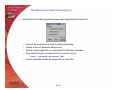
Fluent Tips & Tricks
UGM 2004
Sutikno Wirogo
Samir Rida
1 / 75
Outline
List of Tips and Tricks collected from:
ƒ Solution database available through the Online Technical Support (OTS)
portal
http://www.fluentusers.com
ƒ Frequently Asked Questions
ƒ Know-how of Fluent’s technical staff
This presentation provides Tips and Tricks:
ƒ For IO and Batch
ƒ For Case Set-up and Mesh
ƒ For Solving
ƒ For Post-Processing
ƒ For Reporting
2 / 75
This presentation provides Tips and Tricks:
ƒ For IO and Batch
ƒ For Case Set-up and Mesh
ƒ For Solving
ƒ For Post-Processing
ƒ For Reporting
3 / 75
Miscellaneous on Parallel IO
ƒ In parallel, the mesh is first read into the host and then distributed to the compute nodes
ƒ If reading case into parallel solver takes unusually long time, do the following:
• Merge as many zones as possible
• Put the host and compute-node-0 on the same machine
• Put the case and data files on a disk on the machine running the host and compute-node-0
processes
ƒ Parallel Fluent will allocate buffers for exchanging messages while reading and building the grid
• Default buffer size depends of the case that is being read
For 4 million cell case on 4 CPUs, the buffer size will be 4M/4 = 1M
• To query buffer size, use the following scheme command:
(%query-parallel-io-buffers)
• If the host machine does not have enough memory, using a large buffer will slow down the
read case stage and thus can limit the maximum buffer size using:
(%limit-parallel-io-buffer-size 0)
Needs to be executed before reading the case file
¾ Will increase the total number of messages exchanged but may still give better
performance
• Once the case file has been read, can use the following to reset/free the buffers:
(%allocate-parallel-io-buffers 10000000)
(%query-parallel-io-buffers)
¾
4 / 75
Miscellaneous on Parallel IO
ƒ If the machine running the host process has enough memory, can speed up reading the case
file by using the following Scheme command:
(rpsetvar 'parallel parallel/fast-io? #t)
Fluent will first read the whole mesh into the host machine before distributing to the compute
nodes
ƒ When loading a large mesh into parallel Fluent and the process hangs, execute the
following Scheme command:
(rpsetvar 'parallel/case-read-use-pack? #f)
The above will disable buffer packing and will change the way entities are packed into
messages during the build process
ƒ To check the time taken to read a case, can use:
(print-case-timer)
ƒ Fluent 6.2 has significant improvement for parallel case read
• Two available settings:
(rpsetvar ‘parallel/fast-read-case? #t)
(rpsetvar ‘parallel/fast-read-section? #t)
Gives the similar performance as the fast-io option in Fluent 6.1 but with much less
memory usage
• Turned on by default
• If turned off, will revert to the previous 6.1 methods
5 / 75
Miscellaneous on Batch Processing (1)
ƒ Commands to run in batch mode:
fluent 3d -g < batch.jou >& out.trn &
for C-shell
fluent 3d -g < batch.jou > out.trn 2>&1 &
for Bourne/Korne-shell
fluent 3d -g -i batch.jou –hidden
for windows
For Windows, without –hidden, the GUI will still be started but iconified
ƒ For Windows, there is no option for getting an output file
A transcript file should be started and then stopped before exiting the FLUENT session
ƒ To receive mail notification upon the completion of a batch job, add the following line at the
end of the batch journal:
!mail email-address < message.txt
where message.txt is a text file located inside the working directory and contains the message
to be sent
ƒ To enter a comment inside a journal file:
; This line is commented
ƒ To execute a shell command inside a journal file:
! Shell-command-to-be-executed
ƒ To generate animation files during a batch processing, add the following option to the start up
command of the batch job:
-driver null
6 / 75
Miscellaneous on Batch Processing (2)
ƒ Is it possible to read a journal file from another journal file ?
No. Nested journal files are not allowed in Fluent
ƒ How to execute several batch processes sequentially ?
• In Unix/Linux environments, if a shell command is not ended by an ampersand (&)
then the OS will wait until the completion of the execution of that line before going to
the next line. This is not the case with Windows
• Suppose there are two directories corresponding to two cases where each has its
own corresponding journal file. Then see the following shell scripts:
Unix/Linux
cd ./dir1
fluent 3d -psmpi -t2 -g < batch1.jou
cd ../dir2
fluent 3d -psmpi -t2 -g < batch2.jou
Windows
call cd .\dir1
call fluent 3d -wait -g -i batch1.jou
call cd ..\dir2
call fluent 3d -wait -g -i batch2.jou
7 / 75
Miscellaneous on Batch Processing (3)
ƒ Useful options for batch processing have been implemented in Fluent 6.1
•
•
•
•
Confirm file overwrite is a must for batch processing
Option to turn off question dialog boxes
Must be set through GUI, no equivalent TUI/Scheme command
Equivalent Scheme command to turn on exit on error is:
(set! *cx-exit-on-error* #t)
• Can be appended inside the journal file or .fluent file
8 / 75
Check Pointing (1)
ƒ It is possible to tell the Fluent process to stop the iteration and write the case/data files
without interacting with the GUI
ƒ This procedure is useful to stop a batch process or when the GUI process has crashed, and
can be used as long as Fluent is still in the iteration loop
ƒ In Unix/Linux environment, the owner of the process can create a kill file inside the /tmp
directory:
unix> cd /tmp
unix> touch exit-fluent
exit Fluent after writing files
or
unix> touch check-fluent
continue iteration after writing files
If either exit-fluent or check-fluent found in /tmp, Fluent will finish the current iteration, write
the files, and then delete the exit-fluent or check-fluent file
ƒ The files will be written to the same directory where the original input files were read and
will have the same names but with appended current iteration number
By default, the case file will be written
ƒ To write the data file only, execute the following Scheme command before iterating:
(rpsetvar 'checkpoint/write-case? #f)
9 / 75
Check Pointing (2)
ƒ Make sure that sufficient disk space is available.
• Check-pointing code calls the same file I/O routines used by the GUI or TUI and will
produce the same error messages if disk space is insufficient
• In such case, Fluent will not return to the iteration loop
ƒ The touch command will produce file of zero length and is also available in Windows
ƒ For Windows, the check point files need to be created at:
C:\temp\check-fluent.txt
C:\temp\exit-fluent.txt
ƒ If the machine has several Fluent sessions running, named check pointing can be used
to selectively stop a specific Fluent process
ƒ A specific check point name can be added to the first line of the batch journal file, as
shown below:
(set! checkpoint/exit-filename "/tmp/exit-fluent-job-1")
file/read-case-data sample.cas
solve/iterate 1000
file/write-case-data final.cas
ƒ To stop this particular job, use the following command inside the /tmp directory:
unix> touch exit-fluent-job-1
10 / 75
This presentation provides Tips and Tricks:
ƒ For IO and Batch
ƒ For Case Set-up and Mesh
ƒ For Solving
ƒ For Post-Processing
ƒ For Reporting
11 / 75
The .fluent File (1)
ƒ When FLUENT opens, it auto executes the .fluent file in the:
• home directory of unix users
• C:\ directory of Windows machines
ƒ A .fluent file can contain any number of scheme file names to load
• Note: unless full path is specified for each scheme file in .fluent file, FLUENT tries to
locate the scheme files from the working directory
12 / 75
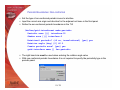
The .fluent File (2)
ƒ Scheme commands can also be appended inside the .fluent file itself
;; ------------------------------------------------------------------------------------------;;
;; Code to create USC panel
(let ((menu (cx-add-menu "USC" #\U)))
(cx-add-item menu "User Services Center" #\O #f and (lambda ()
(system "netscape http://www.fluentusers.com/ &"))))
;; Various useful stuff
(set! *cx-exit-on-error* #f)
;; ------------------------------------------------------------------------------------------;;
USC panel created by
13 / 75
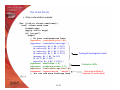
The .fluent File (3)
ƒ Other customization example:
(let ((old-rc client-read-case))
(set! client-read-case
(lambda args
(apply old-rc args)
(if (cx-gui?)
(begin
;; Do your customization here
(rpsetvar 'residuals/plot? #t)
(rpsetvar 'residuals/settings '(
(continuity #t 0 #f 0.001)
(x-velocity #t 0 #f 0.001)
(y-velocity #t 0 #f 0.001)
(z-velocity #t 0 #f 0.001)
(energy #t 0 #f 1e-06)
(k #t 0 #f 0.001)
(epsilon #t 0 #f 0.001)))
(rpsetvar 'mom/relax 0.4)
(rpsetvar 'pressure/relax 0.5)
(rpsetvar 'realizable-epsilon? #t)
(cxsetvar 'vector/style "arrow")
;; You can add more settings here
)))))
}
}
14 / 75
Turning off convergence check
Customize URFs
Use arrow instead of
harpoon for vector head
Creation of Non-conformal Interface (Solution 796)
ƒ Intersected mesh is created using the two interface meshes and then used to
‘replace’ the original interface meshes.
+
„
ƒ Creation of intersected mesh is delicate, if fails, try the alternative schemes by using
either of the following Scheme commands:
(rpsetvar 'nonconformal/cell-faces 0)
(rpsetvar 'nonconformal/cell-faces 2)
The default is (rpsetvar 'nonconformal/cell-faces 1)
ƒ If the interface zones are of different sizes, selecting the smaller interface as Zone 1
is usually more robust
ƒ To create non-conformal interface which crosses periodic boundary, need to set the
following Scheme command first:
(rpsetvar 'nonconformal/allow-interface-at-periodic-boundary 0)
ƒ To improve accuracy and robustness:
• Maintain similar face element sizes at both interfaces
• Maintain good face mesh skewness at both interfaces
15 / 75
Creation of Non-conformal Interface (Solution 928)
ƒ
If the previous workaround for non-conformal interface
creation still fails (e.g. due to too large of gap, etc), can try
to project one interface to the other
ƒ
Write BC file from the current Fluent session.
ƒ
Read the case file into Tgrid
ƒ
Use the TUI command to project one interface to the
other
gap
boundary/project-face-zone interface-1 interface-2
gap eliminated
ƒ
Write a new mesh
ƒ
Use the BC file to resetup the case
ƒ
Recreate the non-conformal interface
elongated cells
16 / 75
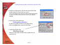
Non-conformal Interface – Periodic Type (Overview and Example)
ƒ The periodic option for the non-conformal interface is used if the non-overlapping
portions of the interface is periodic
Example: Rotor-Stator interaction
{
Stator
}
Rotor
periodic
ƒ This option is not for non-conformal periodic
• Non-conformal periodic setup is done using the TUI commands
17 / 75
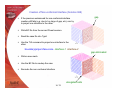
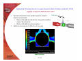
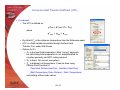
Non-conformal Interface – Coupled Type (Overview and Example)
ƒ The coupled option for the non-conformal interface can
be used to:
• Couple non-matching fluid and solid interface
meshes
• Couple non-matching fluid and fluid interface
meshes and insert a thin wall in between
Example: Canard Rotor Wing (CRW)
External freesteam
Inside interface (fluid)
Induced internal
ƒ Induced internal flow due to wing rotation
ƒ Cooling heat transfer from the external flow
ƒ Internal flow meshes must be fine along the span to
resolve recirculations inside
ƒ External flow meshes can be coarser along the span
Outside interface (solid)
18 / 75
Periodic Boundaries
ƒ Two types:
• Pressure drop occurs across translationally periodic boundaries (e.g. tube bank)
• No Pressure drop occurs across rotationally or translationally periodic boundaries
19 / 75
Periodic Boundaries: Conformal
ƒ To create the periodicity in Fluent, use the TUI command:
grid/modify-zones/make-periodic
• Can make the periodicity either translational or rotational
• The periodicity type of the pair inside the boundary conditional panel
will be updated accordingly
ƒ For rotationally periodic cases, the periodicity axis is specified inside the
fluid zone that contains the periodic pair
ƒ Some Tips:
• If creation fails because of slightly non-matching mesh nodes,
increase the matching tolerance up to 0.5 (default is 0.05) using:
grid/modify-zones/match-tolerance
•
•
To repair corrupted periodic zones:
modify-zone/repair-periodic
• For translationally periodic boundaries, the command computes
an average translation distance and adjusts the node
coordinates on the shadow face zone to match this distance
• For rotationally periodic boundaries, the command prompts for
an angle and adjusts the node coordinates on the shadow face
zone using this angle and the defined rotational axis for the cell
zone
To slit the periodic boundary into two symmetry boundaries use:
grid/modify-zones/slit-periodic
20 / 75
Periodic Boundaries: Non-conformal
ƒ Set the type of non-conformal periodic zones to interface
ƒ Input the correct axis origin and direction for the adjacent cell zone in the fluid panel
ƒ Define the non-conformal periodic boundaries in the TUI
/define/grid-interfaces> make-periodic
Periodic zone [()] interface-15
Shadow zone [()] interface-2
Rotational periodic? (if no, translational) [yes] yes
Rotation angle (deg) [0] 40.0
Create periodic zone? [yes] yes
grid-interface name [] fan-periodic
ƒ The right hand rule must be used when entering the rotation angle value
ƒ With non-conformal periodic boundaries it is not required to specify the periodicity type in the
periodic panel
21 / 75
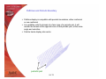
Face Extrusion
ƒ Ability to extrude a boundary face zone and extend the solution domain without having to exit
the solver
• A typical application of the extrusion capability is to extend the solution domain when
recirculating flow is impinging on a flow outlet
ƒ Current extrusion capability creates prismatic or hexahedral layers based on the shape of the
face and normal vectors to the face zone’s nodes.
ƒ New fluid zone is created
ƒ Implemented only in 3D
ƒ Two options available in the TUI:
• Extrude a face thread by specifying a list of displacements (in SI units).
define/boundary-conditions/modify-zone/extrude-face-zone-delta
• Extrude a face thread by specifying a total distance (in SI units) and a list of parametric
locations between 0 and 1 (e.g. 0., 0.1, 0.3, 0.75, 1.0).
define/boundary-conditions/modify-zone/extrude-face-zone-para
22 / 75
Face Extrusion: Example
ƒ A cube (10x10x10) is extruded twice at the outlet by a distance of 1 m
/define/boundary-conditions/modify-zones> extrude-face-zone-delta
Distance delta(1) [()] 1
Distance delta(2) [()] 1
Distance delta(3) [()]
Extrude face zone? [yes]
Moved original zone (outlet) to interior-7
Created new prism cell zone fluid-10
Created new prism cap zone pressure-outlet-11
Created new prism side zone wall-12
Created new prism interior zone interior-13
23 / 75
Miscellaneous on Mesh Modifications (1)
ƒ How to repair left-handed faces in Fluent ?
/grid/modify-zones/repair-face-handedness
Left-handed cells usually occur with highly skewed cells and/or negative volumes.
ƒ What is tfilter ?
A set of utilities used by Fluent/Gambit/Tgrid to perform mesh related modifications, such as:
• Convert mesh to Fluent format
• Convert mesh
• Merge meshes
In recent releases, tfilter has been renamed to utility
Utility can be invoked manually. To find all the options:
shell> utility - h
How to convert 2D mesh into 3D surface mesh ?
utility tconv –d2 sample2d.msh 3d-surface.msh
The z-coordinate is assigned as zero in the 3d surface mesh
ƒ How to convert 3D surface mesh into 2d mesh ?
utility tconv –d3 3d-surface.msh sample2d.msh
The z-coordinate is ignored in the 3d surface mesh
ƒ How to merge two meshes ?
utility tmerge3d -cl -p mesh1.msh mesh2.msh combined.msh
ƒ How to convert CFX mesh to Fluent mesh format ?
utility fe2ram -cl -tCFX -dN -cl -group cfx.geo fl.cas
24 / 75
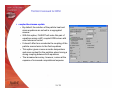
Miscellaneous on Mesh Modifications (2)
ƒ How to delete, deactivate, and activate cell zone(s) from within Fluent ?
Grid „ Zone
ƒ
ƒ
ƒ
ƒ
„ Delete …
„ Deactivate
„ Activate
The face boundaries of a deactivated cell zone will be changed to wall
Works only in serial (not parallelized yet in Fluent 6.1)
Useful to isolate highly skewed cells and remove them from computations
Fluent 6.2 will have the functionality to Add new cell zones
25 / 75
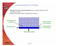
Temperature Definitions for Thin Wall Model
ƒ Thin wall model applies normal conduction only (no in-plane conduction) and no
actual cells are created
ƒ Wall thermal boundary condition is applied at the outer layer
static-temperature
(cell value)
wall-temperature
(outer-surface)
wall-temperature
(inner-surface)
thin wall (no cell)
Wall thermal condition
26 / 75
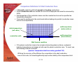
Temperature Definitions for Shell Conduction Zone
ƒ A thin wall conduction with both normal and in-plane conductions
ƒ Actual conduction cells are created but can not be displayed and cannot be accessed by
UDFs
ƒ Solid properties of the conduction zones must be constant and can not be specified as
temperature dependent
ƒ Case must be partitioned in the serial mode before loading into parallel (conduction zones
need to be encapsulated)
wall-temperature
(outer-surface)
static-temperature
(cell value)
wall-temperature
(inner-surface)
conduction cells
Wall thermal condition
ƒ If the planar conduction zone(s) has complex intersecting planar surfaces, unphysical
high/low temperatures can happen at cells near the planar conduction zone. To avoid, use
the following scheme command:
(rpsetvar 'temperature/shell-secondary-gradient? #f)
Will drop the accuracy of the diffusive flux computation in the shell conduction
zone to first order, but should significantly improve the stability of the temperature field.
27 / 75
Alternate Formulation for Wall Temperature
ƒ solve/set/expert/use alternate formulation for wall temperature? [no]
• FLUENT models the flux at the wall as follows:
r
q = k∇T ⋅ n
q=k
(Tw − Tc )
+ f (∆T )
∆h
• The term f(∆T) includes second order terms that need to be determined, which involves
approximations
ƒ solve/set/expert/use alternate formulation for wall temperature? [yes]
• Assume face center is defined such as the vector between cell center and face
center is perpendicular to the wall
r
q = k∇T ⋅ n
q=k
(Tw − Tc )
∆h
• The term f(∆T) vanishes and ∆h changes
• This option doesn’t impact the results if the wall cells are not skewed
28 / 75
define/models/energy?
ƒ include diffusion at inlets?
• The net transport of energy at inlets consists of both the convection and diffusion
components
• The convection component is fixed by the user specified inlet temperature
• The diffusion component, however, depends on the gradient of the computed
temperature field, and thus is not specified a priori
• The default is to include the diffusion of energy at inlets
• To turn off inlet energy diffusion, answer [no] to include diffusion at inlets?
• Available only for the segregated solver
29 / 75
define/models/species/inlet-diffusion?
ƒ inlet-diffusion?
• The net transport of species at inlets consists of both the convection and diffusion
components
• The convection component is fixed by the user specified inlet species concentration
• The diffusion component, however, depends on the gradient of the computed species
concentration field, and thus is not specified a priori
• The default is to include the diffusion flux of species at inlets
• To turn off inlet energy diffusion, answer [no] to include diffusion at inlets?
• Available only with the segregated solver
30 / 75
TUI/GUI Command for DPM
ƒ coupled-heat-mass-update
• By default, the solution of the particle heat and
mass equations are solved in a segregated
manner
• With this option, FLUENT will solve this pair of
equations using a stiff, coupled ODE solver with
error tolerance control
• It doesn’t affect nor accelerate the coupling of the
particle source terms to the fluid equations
• This option gives a more accurate temperature
and mass content for the particles when having a
strong coupling between both equations
• The increased accuracy, however, comes at the
expense of increased computational expense
31 / 75
Modify Rosin-Rammler parameters for atomizers (Solutions 666 & 908)
ƒ By default, the spread parameter for the Rosin Rammler distribution is 3.5 for all the
atomizer models. Is it possible to change this parameter ?
ƒ Can alter this spread parameter through the Text User Interface by executing:
(rpsetvar 'dpm/atomizer-spread-param 3.9)
ƒ For effervescent atomizer, the spread parameter
is hardwired, and can not be changed
ƒ This rp-variable command will work for all
atomizers in FLUENT 6.2
ƒ What about the dispersion angle in the
Flat-Fan atomizer model ?
ƒ The dispersion angle cannot be altered
ƒ It is hardwired to a value of 6 degrees
In FLUENT 6.2, there will be an rp-variable to change it
Gas Flow
Initial
Angle
Inner Diameter
Liquid Flow
Outer
Diameter
Air-Blast Atomizer
32 / 75
This presentation provides Tips and Tricks:
ƒ For IO and Batch
ƒ For Case Set-up and Mesh
ƒ For Solving
ƒ For Post-Processing
ƒ For Reporting
33 / 75
Calculate Radial, Axial and Tangential velocities (Solution 562)
ƒ Only velocities in Cartesian coordinates (Ux,Uy,Uz) are accessible through the UDF
macros
ƒ The radial, tangential, and axial velocities (Ur, Ut, Ua) within a fluid zone can be
computed using a UDF
ƒ An example: implement an energy source term that is a function of the radial velocity
ƒ Each fluid zone will have a user specified axis origin and axis direction vectors
ƒ These two vectors can be queried in UDF by using special macros
ƒ Knowing these two vectors, the radial, tangential, and axial vector (Er,Et,Ea) can be
computed and the cartesian velocities can be dotted with this vector to obtain the radial,
tangential, and axial velocities within that fluid zone
ƒ The selected fluid in the reference panel has no bearing on the macros
34 / 75
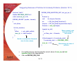
Calculate Radial, Axial and Tangential velocities (Solution 562)
#include "udf.h"
#define FACTOR -950.0
if (rmag != 0.)
{
NV_VS (er,=,r,/,rmag);
NV_CROSS(et, axis, er);
ur = NV_DOT(V,er);
ut = NV_DOT(V,et);
ua = NV_DOT(V,axis);
}
else
{
ur = 0.0;
ut = 0.0;
ua = NV_DOT(V,axis);
}
DEFINE_SOURCE(cell_cold, cell, thread, dS, eqn)
{
real NV_VEC(origin), NV_VEC(axis);
real NV_VEC(V), NV_VEC(r), NV_VEC(R), NV_VEC(B);
real NV_VEC(er), NV_VEC(et);
real xc[ND_ND];
real Bmag, rmag, source;
real ua, ur, ut;
/* Get origin vector of fluid region */
NV_V (origin, =, THREAD_VAR(thread).cell.origin);
/* Get axis of fluid region */
NV_V (axis, =, THREAD_VAR(thread).cell.axis);
/* Store the 3 Cartesian velocity components in vector V */
N3V_D(V, =, C_U(cell,thread),C_V(cell,thread),C_W(cell,thread));
/*source term */
source = FACTOR*ur;
/* Get current cell coordinate */
C_CENTROID(xc,cell,thread);
/* derivative of source term w.r.t. enthalpy */
dS[eqn] = 0.0;
/* Calculate (R) = (Xc)-(Origin) */
NV_VV(R, =, xc, -, origin);
/* Calculate |B| = (R) dot (axis)*/
Bmag = NV_DOT(R,axis);
/* Calculate (B) = |B|*axis */
NV_VS(B,=,axis,*,Bmag);
/* Calculate (r) = (R)-(B) This is the local radial vector*/
NV_VV(r, =, R, -, B);
/* Calculate |r|*/
rmag = NV_MAG(r);
return source;
}
Xc
Ez
R
Origin
r
B
Ey
Ex
Axis
35 / 75
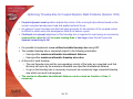
Staggering Releases of Particles for Unsteady Problems (Solution 1017)
ƒ Unsteady DPM injection releases the particle packets at the beginning of every
timestep
ƒ For problem with large elapsed time and small timestep size, many particles will
need to be tracked inside the computational domain
ƒ Tracking large number of particles is computationally expensive (RAM and CPU
time)
ƒ A process can be developed to inject particles at a certain user specified time interval
so as to reduce the number of particles that need to be tracked inside the domain
ƒ The process will inject the particles at the beginning of a timestep and then
store/accumulate the particles’ mass during the next timesteps when injections are
turned off
ƒ At the time of the next injection, the accumulated particles’ mass will be injected
ƒ There will be fewer particles but the particles’s mass will be preserved
36 / 75
Staggering Releases of Particles for Unsteady Problems (Solution 1017)
Example: unsteady silo launch with solid particles injected at nozzle exhaust
Staggered Unsteady Injection
Default Unsteady Injection
37 / 75
Staggering Releases of Particles for Unsteady Problems (Solution 1017)
#include "udf.h"
#define RELEASE_STEP 5e-3
static real sum_inj = 0.0;
DEFINE_ADJUST (update, domain)
{
real pflow;
DEFINE_DPM_INJECTION_INIT (init_prt_tm, I)
{
Particle *p;
real
tm, tmspsz, flowrate;
tm
= RP_Get_Real("flow-time");
tmspsz = RP_Get_Real("physical-time-step");
flowrate = sum_inj/tmspsz;
if ( first_iteration )
{
pflow
= get_mdot_prt(tm);
sum_inj += mdot*tmspsz;
}
loop(p,I->p_init)
{
p->flow_rate = flowrate;
}
}
if ((tm+tmspsz) >= I->unsteady_start)
I->unsteady_start += RELEASE_STEP;
Get the current particle flowrate &
store for later release
sum_inj = 0.0;
}
ƒ
ƒ
Move unsteady_start
forward in time for
next release
Reset storage for mass of
particles
For restart purpose, need to write the current values of sum_inj and last
injection time to the case/data file
Can use DEFINE_RW_FILE
38 / 75
Optimizing Timestep Size for Coupled Dynamic Mesh Problems (Solution 1018)
ƒ Coupled dynamic mesh problem adjusts the motion of the moving body/surfaces based on the
current computed aerodynamic load and applied external forces
ƒ An optimum ‘mean’ timestep size that will apply generally for the duration of the coupled motion
is difficult to obtain since the aerodynamic load is not known a priori
ƒ Continual and manual adjustment of the timestep size is required to avoid using an excessively
conservative value that will increase running time or too large value that will cause the
dynamic remeshing to fail
ƒ It is possible to implement a user defined variable timestep size using UDF
ƒ The variable timestep size is computed subject to the following constraints:
• User specifies maximum allowable translational distance
• User specifies maximum allowable timestep size value
ƒ At the end of each timestep:
• The next timestep size and the corresponding velocity of the body are computed such that
the body will move by the maximum allowable user specified translational distance
• A cap on the timestep size is necessary to prevent an excessively large computed timestep
size which can result in divergence
ƒ The maximum allowable translational distance can be varied as function of time, if
necessary
39 / 75
Optimizing Timestep Size for Coupled Dynamic Mesh Problems (Solution 1018)
ƒ A relation is needed to solve for both the timestep size and velocity of the body which
satisfy the constraint of the specified translational distance of the body
ƒ This relation is obtained by solving a quadratic equation derived from the following two
equations:
hmax = V n +1 × dt
F V n +1 − V n
=
m
dt
hmax
= maximum allowable distance traveled
F
m
= force_acting_on_body/mass_of_body
Vn
= body velocity at previous timestep
V n +1
= body velocity at next timestep
dt
= next timestep size
ƒ The above represents two equations which can be solved for the two unknowns,
V n +1
and
dt
.
40 / 75
Optimizing Timestep Size for Coupled Dynamic Mesh Problems (Solution 1018)
Applied to Dynamic Ball Diverter Valve
ƒ
ƒ
Side inlets
Dynamic ball diverter valve problem requires coupled
dynamic mesh model
ƒ Motion of the ball is controlled by varying the massflow
rates of the side inlets
ƒ Motion of the ball is not known apriori
Optimum timestep size is difficult even to guess
Mach contour
41 / 75
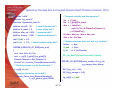
Optimizing Timestep Size for Coupled Dynamic Mesh Problems (Solution 1018)
/* Compute velocity and timestep size */
#include "udf.h"
#include "sg_mem.h"
#include "dynamesh_tools.h“
#define
#define
#define
#define
zoneID
b_mass
dtm_mx
hmove
28
1.0
0.005
0.001
Vn = V_ball;
Fm = f_glob[0]/b_mass;
dtm = ( -fabs(Vn) +
sqrt( Vn*Vn + 4.0*fabs(Fm)*hmove ) )/
( 2.0*fabs(Fm) );
if ( dtm > dtm_mx ) dtm = dtm_mx;
Velx = Vn + Fm*dtm;
/* zone ID for the ball */
/* mass of the ball */
/* maximum delt */
/* maximum distance */
real V_ball = 0.0;
real b_ctr = 0.0; /* center location of the ball */
DEFINE_EXECUTE_AT_END(exec_end)
{
real dtm, Velx, Vn, Fm;
real x_cg[3], f_glob[3], m_glob[3];
Domain *domain = Get_Domain(1);
Thread *tf = Lookup_Thread(domain,zoneID);
/* Get the previous c.g. for the ball zone */
x_cg[0] = b_ctr;
/* Compute the forces on the ball */
Compute_Force_And_Moment(domain,tf,
x_cg,f_glob,m_glob,TRUE);
/* Update velocities, delt, and ball c.g. location */
tmsize = dtm;
V_ball = Velx;
b_ctr += V_ball*tmsize;
RP_Set_Real("physical-time-step",tmsize);
}
DEFINE_CG_MOTION(valve_motion, dt, cg_vel,
cg_omega, time, dtime)
{
NV_S(cg_vel, =, 0.0);
NV_S(cg_omega, =, 0.0);
cg_vel[0] = V_ball;
}
42 / 75
Optimizing Timestep Size for Coupled Dynamic Mesh Problems (Solution 1018)
X_CG comparison
Same approach as applied to the 6 DOF MDM UDF
6
old-x_cg[0]
5
srl-var-x_cg[0]
old-x_cg[1]
srl-var-x_cg[1]
4
old-x_cg[2]
ser-var-x_cg[2]
x_cg (m)
3
2
1
0
0
0.1
0.2
0.3
0.4
0.5
0.6
0.7
-1
-2
time (s)
VEL_CG comparison
12
fix v_cg[0]
var v_cg[0]
10
fix v_cg[1]
var v_cg[1]
8
fix v_cg[2]
var v_cg[2]
• Time to solution with fixed timestep size
on a single CPU is 3 days
• With variable timestep size is about 2 days
vel_cg (m/s)
6
4
2
0
0
0.1
0.2
0.3
0.4
-2
-4
time (s)
43 / 75
0.5
0.6
0.7
Achieving a Target Thrust at Nozzle Exit (Solution 718)
ƒ External aero configuration of a full aircraft with wing-body-pylon-nacelle requires the
specifications of target massflow rate at the nacelle inlet and target thrust at the nozzle
exit
ƒ Target massflow rate is specified using massflow-outlet boundary type (UDF, Fluent 6.1).
ƒ Target thrust can be achieved by manually adjusting the inlet total-temperature
Specify target thrust
Adjust total temperature
Specify target massflow rate
UDF, Scheme, Fluent 6.1
ƒ The user manual adjustment can be automated by a UDF
ƒ Total temperature adjustment at each iteration is computed based on the equation
relating the total temperature to the thrust
44 / 75
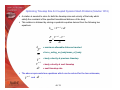
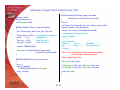
Achieving a Target Thrust at Nozzle Exit (718)
ƒ A calculated update of the total temperature to achieve the target thrust is needed to
ensure fast and robust procedure (as opposed to using a shooting method)
2
Th = m& Ve Ve =
Tt
γ − 1 Ve
=1 +
T
2 a2
2
Th
ρA
}
d Tt
γ −1 1
Tt
γ −1 1
=
+
d Th
1
=1 +
Th Ä
Ä
2
2
T
2 ρ Aa
2 ρ Aa
T
ƒ An example showing the convergence of the process starting with thrust of 880N to achieve a
target thrust of 1200N (30 iterations)
45 / 75
Achieving a Target Thrust at Nozzle Exit (718)
real dTCompute(real Thrust_target, real alpha,
real Ttot_min, real Ttot_max, int zoneID)
{
face_t f;
real Temp, Ttot, VsoundSq, rho, area, Thrust_present, dTot;
Domain *domain = Get_Domain(1);
Thread *tf = Lookup_Thread(domain,zoneID);
#include “udf.h”
#define Gamma 1.4
real Ttot_new = 200.0;
DEFINE_ADJUST (Thrust_compute, domain)
{
real Thrust_target, alpha, Ttot_min, Ttot_max;
Thrust_target = 1200.0;
alpha
= 0.5;
Ttot_min = 20.0;
Ttot_max = 1000.0;
/* Compute zone average values */
begin_f_loop(f,tf)
{ …. }
end_f_loop(f,tf)
Temp = … ;
Ttot = … ;
VsoundSq
=…;
rho = … ;
area = … ;
Thrust_present = … ;
/* Finish */
/* Target thrust in Newton */
/* Relaxation */
/* Min Ttot in K */
/* Max Ttot in K */
zoneID = THREAD_ID(tf);
Ttot_new = dTCompute(Thrust_target,alpha,
Ttot_min,Ttot_max,zoneID);
dTot = 1.0 + 0.5*(Gamma-1.0)/ ( rho*area*VsoundSq )*
(Thrust_target - Thrust_present )/
dTtot = alpha*Temp*dTot;
}
DEFINE_PROFILE (Thrust_fix, tf, position)
{
face_t f;
begin_f_loop(f,tf)
F_PROFILE(f,tf,position) = Ttot_new;
end_f_loop(f,tf)
Ttot_new = Ttot + dTtot;
if ( Ttot_new >= Ttot_max ) Ttot_new = Ttot_max;
if ( Ttot_new <= Ttot_min ) Ttot_new = Ttot_min;
return Ttot_new;
}
}
46 / 75
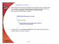
Miscellaneous on UDF (1)
ƒ Define Adjust UDF is called at the beginning of every iteration even for unsteady solver.
ƒ For unsteady runs, there are instances where it is desirable for the Adjust UDF to be
called only at the beginning of the first iteration of every time-step.
ƒ Can use the macro first-iteration, example:
DEFINE_ADJUST(myadjust, domain)
{
if (first_iteration)
{
/* Do procedures to be executed only at the first
iteration of every timestep */
}
}
ƒ An alternative is to use the Execute At End UDF which is called at the end of every
iteration (steady) or timestep (unsteady).
47 / 75
Miscellaneous on UDF (2)
ƒ Certain fields inside the FLUENT model panel do not have built-in UDF hookups, thus
it is difficult to specify user specified time/iteration varying values
ƒ Examples are the wall and fluid speeds
ƒ Is there any workaround ?
No UDF hookup
48 / 75
Miscellaneous on UDF (3)
ƒ Can write a DEFINE_ADJUST UDF and directly access the macro of the variable of
interest (contact support engineer for variable names)
THREAD_VAR(tf).wall.origin[0]
THREAD_VAR(tf).wall.origin[1]
THREAD_VAR(tf).wall.origin[2]
THREAD_VAR(tc).fluid.origin[0]
THREAD_VAR(tc).fluid.origin[1]
THREAD_VAR(tc).fluid.origin[2]
THREAD_VAR(tf).wall.axis[0]
THREAD_VAR(tf).wall.axis[1]
THREAD_VAR(tf).wall.axis[2]
THREAD_VAR(tc).fluid.axis[0]
THREAD_VAR(tc).fluid.axis[1]
THREAD_VAR(tc).fluid.axis[2]
THREAD_VAR(t1).fluid.velocity[0]
THREAD_VAR(t1).fluid.velocity[1]
THREAD_VAR(t1).fluid.velocity[2]
THREAD_VAR(tf).wall.translate_mag
THREAD_VAR(tf).wall.translate_dir[0]
THREAD_VAR(tf).wall.translate_dir[1]
THREAD_VAR(tf).wall.translate_dir[2]
THREAD_VAR(tc).fluid.omega
THREAD_VAR(tf).wall.omega
THREAD_VAR(tf).wall.u
THREAD_VAR(tf).wall.v
THREAD_VAR(tf).wall.w
49 / 75
This presentation provides Tips and Tricks:
ƒ For IO and Batch
ƒ For Case Set-up and Mesh
ƒ For Solving
ƒ For Post-Processing
ƒ For Reporting
50 / 75
Saving Adaption Register for subsequent use (Solution 617)
ƒ The adaption register information is not stored either in case or data files. The information is
lost upon saving and reopening the case/data files
ƒ There is no direct way to preserve the register for subsequent use
ƒ To preserve the information in the register, create a User Defined Scalar (UDS) storage,
initialize/patch the UDF value for all the cells in the domain with 0, and then patch the value of
1 in all the cells of the register. The overall procedure is:
1.
2.
3.
4.
Generate the register by any means (Boundary, Gradient, Iso-Value, Region...)
Define a UDS
Patch the UDS with 0 for all cells in the domain
Patch the UDS with 1 for all the registers that you want to keep (use the number 2, 3, 4… if
you have a second, third, fourth… register, respectively)
5. When the case is saved, the UDS will remain in the database
6. Open the case again and regenerate the register by using Iso-Value Adaption with UDS
values between 0.9 and 1.1
51 / 75
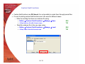
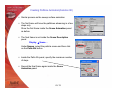
Custom Field Functions
ƒ Custom field functions are GUI based, it is not possible to create them through journal files
ƒ If a set of existing custom field functions are to be used for different cases:
• Write the existing functions as a scheme file using:
¾ Define „ Custom Field Functions „ Manage „ Save
GUI
¾ file/write-field-functions
TUI
•
Read the scheme file to the new case using:
¾ Define „ Custom Field Functions „ Manage „ Load
¾ file/read-field-functions
52 / 75
GUI
TUI
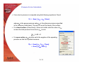
Customizing the Color Map ? (1)
ƒ It is possible to read a custom color map
or write an existing one
ƒ The procedure consists of:
• Loading the Scheme file:
(load “rw-colormap.scm”)
• Reading a new color map:
/file/read-colormap
• Writing an existing color map:
/file/write-colormap
ƒ Example: Static pressure variation for a simple
duct.
Default FLUENT color map
53 / 75
R
("thermacam"
(0.0
(0.083
(0.167
(0.250
(0.333
(0.417
(0.500
(0.583
(0.667
(0.750
(0.833
(0.917
(1.000
)
0.000
0.055
0.306
0.545
0.725
0.824
0.898
0.945
0.973
0.996
0.996
1.000
1.000
G
0.000
0.000
0.000
0.000
0.016
0.114
0.267
0.404
0.545
0.702
0.847
0.945
1.000
Thermacam color map
B
0.000)
0.467)
0.592)
0.616)
0.584)
0.455)
0.098)
0.012)
0.000)
0.000)
0.047)
0.455)
0.976)
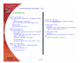
Customizing the Color Map ? (2)
rw-colormap.scm
(define (write-cmap fn)
(let ((port (open-output-file (cx-expand-filename
fn)))
(cmap (cxgetvar 'def-cmap)))
(write (cons cmap (cx-get-cmap cmap)) port)
(newline port)
(close-output-port port)))
(define (read-cmap fn)
(if (file-exists? fn)
(let ((cmap (read (open-input-file (cx-expandfilename fn)))))
(cx-add-cmap (car cmap) (cons (length (cdr
cmap)) (cdr cmap)))
(cxsetvar 'def-cmap (car cmap)))
(cx-error-dialog
(format #f "Macro file ~s not found." fn))))
(define (ti-write-cmap)
(let ((fn (read-filename "colormap filename"
"cmap.scm")))
(if (ok-to-overwrite? fn)
(write-cmap fn))))
54 / 75
(define (ti-read-cmap)
(read-cmap (read-filename "colormap filename"
"cmap.scm")))
(ti-menu-insert-item!
file-menu
(make-menu-item "read-colormap" #t ti-read-cmap
"Read a colormap from a file."))
(ti-menu-insert-item!
file-menu
(make-menu-item "write-colormap" #t ti-writecmap
"Write a colormap to a file."))
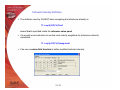
How to save graphics/GUI layout ?
ƒ To save custom window layout, can use the GUI command:
File „ Save Layout
ƒ Sizes and locations of currently defined windows (0,1,2,...) as well as other
windows for iteration panel, display panel, etc that have been opened will be
saved in .cxlayout located at the same location as the .fluent file
55 / 75
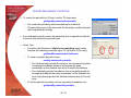
How to create an iso-surface that passes through a selected cell zone?
ƒ The domain has several fluid zones and the objective is to create an iso-surface that
passes through one specific fluid zone
fluid-in
fluid-out
fluid-core
ƒ Create an iso-surface that passes through the entire domain
Surface „ Iso-Surface…
Iso-surface
passing through
the whole domain
56 / 75
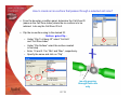
How to create an iso-surface that passes through a selected cell zone?
ƒ From the boundary condition panel, determine the Cell Zone ID
(same as the Cell Zone Index) where the iso-surface is to be
retained. Lets say the Cell Zone ID is 2.
ƒ Clip the iso-surface using to the desired ID:
Surface „ Iso-Clip…
• Under “Clip To Values Of” select “Cell Info”
and “Cell Zone Index”
• Under “Clip Surface” select the surface created
in first step
• Enter 1.9 and 2.1 for “Min” and “Max”, respectively.
• Specify the name and click on “Clip”
iso-clip passing
through fluid-core
only
57 / 75
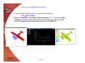
Creating Sweep Surface Animation (Solution 870)
ƒ
ƒ
Display „ Sweep Surface… allows a sweep surface to be defined along an axis and
the resulting sweep animation displayed in the graphics window
No functionality within this panel to save the animation as hardcopy files
Total pressure at tip wake for the M6 wing
ƒ
It is possible to create animation files for the sweep surface using Scene Animation
58 / 75
Creating Sweep Surface Animation (Solution 870)
ƒ Create the surface where the animation sweep will start.
Can use iso-surface/iso-clip-surface but not bounded-planesurface. Surface must be normal to any of the coordinate axis
(e.g. x-axis or yz-plane).
ƒ Display the contour/vector variable on this surface
Display „ Contours…
Set the appropriate contour range and grid display
ƒ Set this contour/vector display as the first key frame
Display „ Scene Animation…
Click on the Add button to enter the frame
ƒ Setup the final frame of the animation sweep
Display „ Scene…
Under Names, select the contour and then click on the
IsoValue button
59 / 75
Creating Sweep Surface Animation (Solution 870)
ƒ Inside the IsoValue panel, enter the final value of the frame
location along the chosen axis (e.g. x-axis)
Click on the Apply button and the surface will be automatically
moved to the final location and the contour/vector display
updated
ƒ Set this frame as the final frame
Display „ Scene Animation…
Increase the number of frames to the desired value
Click on the Add button to enter the final frame
ƒ Create the animation files
Write/Record Format
Option to create either animation files or graphic files (tif,
postscript, etc)
60 / 75
Creating Sweep Surface Animation (Solution 870)
In plane velocity at tip wake for the M6 wing
61 / 75
Creating Pathline Animation (Solution 90)
ƒ Display „ Pathlines… allows pathlines to be released and the resulting
animation displayed in the graphics window
ƒ No functionality within this panel to save the animation as hardcopy files
ƒ It is possible to create animation files for pathlines using Scene Animation
62 / 75
Creating Pathline Animation(Solution 90)
ƒ Similar process as the sweep surface animation
ƒ The first frame will have the pathlines advancing in a few
steps only
Store the first frame inside the Scene Animation panel
as before
ƒ The final frame is set inside the Scene Description
panel
Display „ Scene…
Under Names, select the particle scene and then click
on the Path Attr button
ƒ Inside the Path Attr panel, specify the maximum number
of steps
ƒ Record the final frame again inside the Scene
Animation panel
63 / 75
Pathlines and Periodic Boundary
ƒ Pathline display is compatible with periodic boundaries, either conformal
or non-conformal
ƒ As a pathline exits the domain at a face zone of a periodic pair, it will
reenter the domain at the opposite zone of that periodic pair, at the same
angle and velocities
ƒ Particle tracks display also works
periodic pair
64 / 75
This presentation provides Tips and Tricks:
ƒ For IO and Batch
ƒ For Case Set-up and Mesh
ƒ For Solving
ƒ For Post-Processing
ƒ For Reporting
65 / 75
Mass and Energy flux imbalance in DPM problems (Solution 547)
ƒ In DPM problems, the Report „ Fluxes... panel will usually give a non-zero mass and energy
balances
ƒ The energy imbalance happens with cases involving combustion or heat transfer from the
particles/droplets to the gas phase
ƒ In these cases the user should go to:
Report „ Volume Integrals „ Sum „ Discrete Phase Model… and calculate the sum for:
• DPM Mass Source
• DPM Enthalpy Source
ƒ At convergence, the Sum of DPM Mass Source and DPM Enthalpy Source should be
algebraically equal to the Mass and Total Heat Transfer Rate imbalances in the
Report „ Fluxes… panel
ƒ For large combustion problems, this energy balance can take longer to achieve and is a
better indication of convergence than low residuals
66 / 75
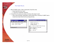
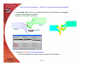
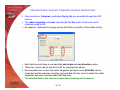
TUI reports surface integrals in SI units only (Solution 845)
ƒ The values of Surface Integrals and Flux Reports are always reported in SI units when
accessed through the Text User Interface (TUI) while they are reported in the userspecified units in the Graphic User Interface (GUI)
ƒ Workaround: Use a function which will convert the value from SI units to the user specified
units for the desired variable
kg/s
lbm/s
ƒ In the example above, the mass-flow rate value is 1.3142 kg/s but the user is interested in
lbm/s, which is the user specified unit in the GUI. The following function can be used:
(to-user-units 1.3142 'mass-flow)
ƒ In order to use this function for other variables, “mass-flow” should be replaced by
the desired variable (e.g. temperature, velocity, length, etc)
67 / 75
Convective Heat Transfer Coefficient (HTC)
ƒ Flux-based
• The HTC is defined as
q”total = h”total ( Tw - Tref )
where
q”total = qrad + qconv
• By default Tref is the reference temperature from the Reference panel
• HTC is a field variable accessible through Surface Heat
Transfer Coe. under Wall Fluxes
• Options for Tref
¾ Tref is the local bulk temperature: Most “correct” approach,
but calculating bulk temperature is not straightforward for
complex geometry and UDF coding required
¾ Tref is fixed: Not correct everywhere
¾ Tref is adjacent cell temperature. It can be done using
Custom Field Function of:
(Total Heat Surface Heat Flux - Radiation Heat Flux)/
(Wall Temperature (Outer Surface) - Static Temperature)
and plotting without node values
68 / 75
Convective Heat Transfer Coefficient (HTC)
ƒ Based on wall functions
(Tw − TP )ρ c p C µ 4 k P 2
1
∗
T ≡
1
q& ′′
1
h = q" /(Tw − TP ) =
Pr y ∗

=  1

∗
Prt  κ ln Ey + P 

 
( )
(y
(y
∗
∗
< yT∗
> yT∗
)
)
1
ρ c pCµ 4 k P 2
T*
• This requires only to run turbulence equations
• The heat flux is q” is the convective flux only
• It would be equivalent to using the adjacent cell as reference temperature in the fluxbased HTC
• Generally, for accurate h, we want TP to be close to the bulk temperature
• This can be achieved only if y+ is large
Tbulk
Tbulk
TP
Tw
Tw
69 / 75
TP
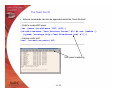
Reporting – Heat Flux and HTC
ƒ Heat flux report:
ƒ It is recommended that you perform
a heat balance check to ensure that
your solution is truly converged
ƒ Exporting Heat Flux Data:
• It is possible to export heat flux data on wall zones
(including radiation) to a generic file
• Use the text interface:
file/export/custom-heat-flux
• File format for each selected face zone:
zone-name nfaces
x_f y_f z_f A
…
Q
T_w
T_c
70 / 75
HTC
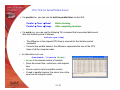
Species and UDS reports
ƒ report/species-mass-flow
• Print list of species mass flow rate at inlets and outlets
• Available after performing 1 iteration
ƒ report/uds-flow
• Print list of user-defined scalar flow rate at boundaries
ƒ These options are more accurate than surface integrals
at boundary zones since no interpolation is used and
corresponds to:
Report „ Fluxes…
in the GUI for mass and heat transfer rates
71 / 75
Pressure Force Calculation
ƒ Force due to pressure is computed using the following equation in Fluent:
Fp = Sum [ ( pg – pref )*Area]
where pg is the gauge pressure and pref is the reference pressure specified
in the reference value panel. The sum is over all the faces of the surface.
ƒ For closed surface (closed body), it does not matter what the value of pref
is since the total pressure force due to pref is zero:
r r
∫ pref n ⋅ dA = 0
ƒ For open surface, pref must be set to the negative of the operating
pressure so that the equation becomes:
Fp = Sum [( pg + pop )*Area]
= Sum [( pabs*Area )]
72 / 75
Turbulent Intensity Definition
ƒ The definition used by FLUENT when computing the turbulence intensity is:
TI = sqrt( (2/3)*k )/Vref
where Vref is specified inside the reference value panel
ƒ It is usually more instructive to use the local velocity magnitude for turbulence intensity
calculation:
TI = sqrt( (2/3)*k )/Vmag-local
ƒ Can use a custom field function to define modified turbulent intensity
73 / 75
CPU Time for Serial/Parallel Solver
ƒ For parallel run, one can use the built-in parallel timer via the GUI:
Parallel „ Timer „ Reset
Parallel „ Timer „ Usage
Before iterating
After completing iterations
ƒ For serial run, you can use the following TUI command that is executed before and
after the iteration period of interest:
(solver-cpu-time)
• The difference is the elapsed CPU time in seconds for the iteration period
completed
• If used in the parallel session, the difference represents the sum of the CPU
times of all the compute nodes
ƒ An alternative is to use:
(benchmark ‘(iterate Niter))
• Niter is the desired number of iteration
• Gives the solver time, cortex time, and elapsed
time
• Can be used in serial or parallel session
• If used in parallel session, the solver time is the
sum from all compute nodes
74 / 75
Thank you !
Thinking CFD ... Think Fluent !
Care to use the very best in CFD
75 / 75