1
VWF
User’s Manual
Silvaco, Inc.
4701 Patrick Henry Drive, Bldg. 2
Santa Clara, CA 95054
Phone
(408) 567-1000
Web:
www.silvaco.com
June 13, 2014
Notice
The information contained in this document is subject to change without notice.
Silvaco, Inc. MAKES NO WARRANTY OF ANY KIND WITH REGARD TO THIS
MATERIAL, INCLUDING, BUT NOT LIMITED TO, THE IMPLIED WARRANTY
OF FITNESS FOR A PARTICULAR PURPOSE.
Silvaco, Inc. shall not be held liable for errors contained herein or for incidental or
consequential damages in connection with the furnishing, performance, or use of this
material.
This document contains proprietary information, which is protected by copyright laws of the
United States. All rights are reserved. No part of this document may be photocopied,
reproduced, or translated into another language without the prior written consent of Silvaco
Inc.
AccuCell, AccuCore, Athena, Athena 1D, Atlas, Blaze, C-Interpreter, Catalyst AD, Catalyst
DA, Clarity RLC, Clever, Clever Interconnect, Custom IC CAD, DeckBuild, DevEdit,
DevEdit 3D, Device 3D, DRC Assist, Elite, Exact, Expert, Expert C++, Expert 200,
ExpertViews, Ferro, Gateway, Gateway 200, Giga, Giga 3D, Guardian, Guardian DRC,
Guardian LVS, Guardian NET, Harmony, Hipex, Hipex C, Hipex NET, Hipex RC,
HyperFault, Interconnect Modeling, IWorkBench, Laser, LED, LED 3D, Lisa, Luminous,
Luminous 3D, Magnetic, Magnetic 3D, MaskViews, MC Etch & Depo, MC Device, MC
Implant, Mercury, MixedMode, MixedMode XL, MultiCore, Noise, OLED, Optolith,
Organic Display, Organic Solar, OTFT, Quantum, Quantum 3D, Quest, RealTime DRC, REM
2D, REM 3D, SEdit, SMovie, S-Pisces, SSuprem 3, SSuprem 4, SDDL, SFLM, SIPC, SiC,
Silvaco, Silvaco Management Console, SMAN, Silvaco Relational Database, Silos,
Simulation Standard, SmartSpice, SmartSpice 200, SmartSpice API, SmartSpice Debugger,
SmartSpice Embedded, SmartSpice Interpreter, SmartSpice Optimizer, SmartSpice RadHard,
SmartSpice Reliability, SmartSpice Rubberband, SmartSpice RF, SmartView, SolverLib,
Spayn, SpiceServer, Spider, Stellar, TCAD Driven CAD, TCAD Omni, TCAD Omni Utility,
TCAD & EDA Omni Utility, TFT, TFT 3D, Thermal 3D, TonyPlot, TonyPlot 3D, TurboLint,
Universal Token, Universal Utility Token, Utmost III, Utmost III Bipolar, Utmost III Diode,
Utmost III GaAs, Utmost III HBT, Utmost III JFET, Utmost III MOS, Utmost III MultiCore,
Utmost III SOI, Utmost III TFT, Utmost III VBIC, Utmost IV, Utmost IV Acquisition
Module, Utmost IV Model Check Module, Utmost IV Optimization Module, Utmost IV
Script Module, VCSEL, Verilog-A, Victory, Victory Cell, Victory Device, Victory Device
Single Event Effects, Victory Process, Victory Process Advanced Diffusion & Oxidation,
Victory Process Monte Carlo Implant, Victory Process Physical Etch & Deposit, Victory
Stress, Virtual Wafer Fab, VWF, VWF Automation Tools, VWF Interactive Tools, and Vyper
are trademarks of Silvaco, Inc.
All other trademarks mentioned in this manual are the property of their respective owners.
Copyright © 1984 - 2014, Silvaco, Inc.
2
VWF User’s Manual
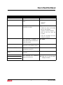
How to Read this Manual
Style Conventions
Font Style/Convention
Description
Example
•
This represents a list of items or
terms.
•
•
•
1.
This represents a set of directions
to perform an action.
To open a door:
1. Unlock the door by inserting
the key into keyhole.
2. Turn key counter-clockwise.
3. Pull out the key from the
keyhole.
4. Grab the doorknob and turn
clockwise and pull.
This represents a sequence of
menu options and GUI buttons to
perform an action.
FileOpen
Courier
This represents the commands,
parameters, and variables syntax.
HAPPY BIRTHDAY
Times Roman Bold
This represents the menu options
and buttons in the GUI.
File
New Century
Italics
This represents the variables of
equations.
x+y=1
2.
3.
Note:
Schoolbook
This represents the additional
important information.
3
Bullet A
Bullet B
Bullet C
Note: Make sure you save often when
working on a manual.
VWF User’s Manual
Table of Contents
Chapter 1
Introduction . . . . . . . . . . . . . . . . . . . . . . . . . . . . . . . . . . . . . . . . . . . . . . . . . . . . . . . . . . . . . .8
1.1 What is Virtual Wafer Fab (VWF) . . . . . . . . . . . . . . . . . . . . . . . . . . . . . . . . . . . . . . . . . . . . . . . . . . . . . . . . . . 9
1.1.1 Advantages . . . . . . . . . . . . . . . . . . . . . . . . . . . . . . . . . . . . . . . . . . . . . . . . . . . . . . . . . . . . . . . . . . . . . . . . 9
1.1.2 Applications . . . . . . . . . . . . . . . . . . . . . . . . . . . . . . . . . . . . . . . . . . . . . . . . . . . . . . . . . . . . . . . . . . . . . . . . 9
1.2 Features . . . . . . . . . . . . . . . . . . . . . . . . . . . . . . . . . . . . . . . . . . . . . . . . . . . . . . . . . . . . . . . . . . . . . . . . . . . . . 10
1.2.1 Database . . . . . . . . . . . . . . . . . . . . . . . . . . . . . . . . . . . . . . . . . . . . . . . . . . . . . . . . . . . . . . . . . . . . . . . . . 10
1.2.2 User-Friendly . . . . . . . . . . . . . . . . . . . . . . . . . . . . . . . . . . . . . . . . . . . . . . . . . . . . . . . . . . . . . . . . . . . . . . 10
1.2.3 Experimental Design . . . . . . . . . . . . . . . . . . . . . . . . . . . . . . . . . . . . . . . . . . . . . . . . . . . . . . . . . . . . . . . . 10
1.2.4 Optimization . . . . . . . . . . . . . . . . . . . . . . . . . . . . . . . . . . . . . . . . . . . . . . . . . . . . . . . . . . . . . . . . . . . . . . 10
1.2.5 Network Execution . . . . . . . . . . . . . . . . . . . . . . . . . . . . . . . . . . . . . . . . . . . . . . . . . . . . . . . . . . . . . . . . . 10
1.2.6 Security Features . . . . . . . . . . . . . . . . . . . . . . . . . . . . . . . . . . . . . . . . . . . . . . . . . . . . . . . . . . . . . . . . . . 11
1.2.7 Scripting Interface . . . . . . . . . . . . . . . . . . . . . . . . . . . . . . . . . . . . . . . . . . . . . . . . . . . . . . . . . . . . . . . . . . 11
1.3 Simulators . . . . . . . . . . . . . . . . . . . . . . . . . . . . . . . . . . . . . . . . . . . . . . . . . . . . . . . . . . . . . . . . . . . . . . . . . . . 12
Chapter 2
Installation . . . . . . . . . . . . . . . . . . . . . . . . . . . . . . . . . . . . . . . . . . . . . . . . . . . . . . . . . . . . . .13
2.1 VWF Variants. . . . . . . . . . . . . . . . . . . . . . . . . . . . . . . . . . . . . . . . . . . . . . . . . . . . . . . . . . . . . . . . . . . . . . . . . 14
2.2 Installing the VWF TAR file . . . . . . . . . . . . . . . . . . . . . . . . . . . . . . . . . . . . . . . . . . . . . . . . . . . . . . . . . . . . . 15
2.3 VWF Modes . . . . . . . . . . . . . . . . . . . . . . . . . . . . . . . . . . . . . . . . . . . . . . . . . . . . . . . . . . . . . . . . . . . . . . . . . . 17
2.3.1 File Mode . . . . . . . . . . . . . . . . . . . . . . . . . . . . . . . . . . . . . . . . . . . . . . . . . . . . . . . . . . . . . . . . . . . . . . . . 17
2.3.2 Database Mode . . . . . . . . . . . . . . . . . . . . . . . . . . . . . . . . . . . . . . . . . . . . . . . . . . . . . . . . . . . . . . . . . . . . 17
2.3.3 Single Machine Queue Mode . . . . . . . . . . . . . . . . . . . . . . . . . . . . . . . . . . . . . . . . . . . . . . . . . . . . . . . . . 28
2.3.4 DRMAA mode . . . . . . . . . . . . . . . . . . . . . . . . . . . . . . . . . . . . . . . . . . . . . . . . . . . . . . . . . . . . . . . . . . . . . 29
Chapter 3
Using the VWF GUI . . . . . . . . . . . . . . . . . . . . . . . . . . . . . . . . . . . . . . . . . . . . . . . . . . . . . . .30
3.1 Overview . . . . . . . . . . . . . . . . . . . . . . . . . . . . . . . . . . . . . . . . . . . . . . . . . . . . . . . . . . . . . . . . . . . . . . . . . . . . 31
3.2 Examples Shipped with VWF. . . . . . . . . . . . . . . . . . . . . . . . . . . . . . . . . . . . . . . . . . . . . . . . . . . . . . . . . . . . 32
3.2.1 Creating the vwf_examples Database . . . . . . . . . . . . . . . . . . . . . . . . . . . . . . . . . . . . . . . . . . . . . . . . . . 32
3.2.2 Loading Examples into an Existing Database . . . . . . . . . . . . . . . . . . . . . . . . . . . . . . . . . . . . . . . . . . . . . 32
3.2.3 Opening Examples in filemode . . . . . . . . . . . . . . . . . . . . . . . . . . . . . . . . . . . . . . . . . . . . . . . . . . . . . . . . 32
3.3 Main GUI components . . . . . . . . . . . . . . . . . . . . . . . . . . . . . . . . . . . . . . . . . . . . . . . . . . . . . . . . . . . . . . . . . 33
3.3.1 Main Window . . . . . . . . . . . . . . . . . . . . . . . . . . . . . . . . . . . . . . . . . . . . . . . . . . . . . . . . . . . . . . . . . . . . . . 33
3.3.2 Creating a New Experiment . . . . . . . . . . . . . . . . . . . . . . . . . . . . . . . . . . . . . . . . . . . . . . . . . . . . . . . . . . 53
3.3.3 Experiment Editor . . . . . . . . . . . . . . . . . . . . . . . . . . . . . . . . . . . . . . . . . . . . . . . . . . . . . . . . . . . . . . . . . . 56
3.3.4 Formatting Cells in the Worksheet . . . . . . . . . . . . . . . . . . . . . . . . . . . . . . . . . . . . . . . . . . . . . . . . . . . . . 72
3.3.5 Defining Splits . . . . . . . . . . . . . . . . . . . . . . . . . . . . . . . . . . . . . . . . . . . . . . . . . . . . . . . . . . . . . . . . . . . . . 76
Chapter 4
Customizing VWF – Preferences Panel . . . . . . . . . . . . . . . . . . . . . . . . . . . . . . . . . . . . .101
4
VWF User’s Manual
Table of Contents
Chapter 5
Tutorial. . . . . . . . . . . . . . . . . . . . . . . . . . . . . . . . . . . . . . . . . . . . . . . . . . . . . . . . . . . . . . . .119
5.1 Prerequisites . . . . . . . . . . . . . . . . . . . . . . . . . . . . . . . . . . . . . . . . . . . . . . . . . . . . . . . . . . . . . . . . . . . . . . . . 120
5.2 Typical VWF Toolchain. . . . . . . . . . . . . . . . . . . . . . . . . . . . . . . . . . . . . . . . . . . . . . . . . . . . . . . . . . . . . . . . 121
5.3 Starting the VWF Software. . . . . . . . . . . . . . . . . . . . . . . . . . . . . . . . . . . . . . . . . . . . . . . . . . . . . . . . . . . . . 122
5.4 Defining a New Experiment . . . . . . . . . . . . . . . . . . . . . . . . . . . . . . . . . . . . . . . . . . . . . . . . . . . . . . . . . . . . 123
5.5 Running an Experiment . . . . . . . . . . . . . . . . . . . . . . . . . . . . . . . . . . . . . . . . . . . . . . . . . . . . . . . . . . . . . . . 141
5.6 Exporting Data From VWF . . . . . . . . . . . . . . . . . . . . . . . . . . . . . . . . . . . . . . . . . . . . . . . . . . . . . . . . . . . . . 148
5.7 Exporting Worksheet . . . . . . . . . . . . . . . . . . . . . . . . . . . . . . . . . . . . . . . . . . . . . . . . . . . . . . . . . . . . . . . . . 149
5.8 Exporting Optimization Results . . . . . . . . . . . . . . . . . . . . . . . . . . . . . . . . . . . . . . . . . . . . . . . . . . . . . . . . 150
5.9 Importing Data into VWF . . . . . . . . . . . . . . . . . . . . . . . . . . . . . . . . . . . . . . . . . . . . . . . . . . . . . . . . . . . . . . 151
5.10 Importing Worksheet Data to Define a DOE . . . . . . . . . . . . . . . . . . . . . . . . . . . . . . . . . . . . . . . . . . . . . . 154
5.11 Sending Worksheet to SPAYN. . . . . . . . . . . . . . . . . . . . . . . . . . . . . . . . . . . . . . . . . . . . . . . . . . . . . . . . . 158
5.12 VWF File Mode . . . . . . . . . . . . . . . . . . . . . . . . . . . . . . . . . . . . . . . . . . . . . . . . . . . . . . . . . . . . . . . . . . . . . 161
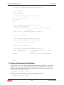
5.13 Using VWF to Run SmartSpice Simulations . . . . . . . . . . . . . . . . . . . . . . . . . . . . . . . . . . . . . . . . . . . . . 166
5.13.1 Preparing the Circuit . . . . . . . . . . . . . . . . . . . . . . . . . . . . . . . . . . . . . . . . . . . . . . . . . . . . . . . . . . . . . . 166
5.14 Running SPICE Simulations for 27 Conditions and Review
the Results Using VWF . . . . . . . . . . . . . . . . . . . . . . . . . . . . . . . . . . . . . . . . . . . . . . . . . . . . . . . . . . . . . . 169
Chapter 6
Optimization in VWF . . . . . . . . . . . . . . . . . . . . . . . . . . . . . . . . . . . . . . . . . . . . . . . . . . . . .178
6.1 Supported Optimization Algorithms . . . . . . . . . . . . . . . . . . . . . . . . . . . . . . . . . . . . . . . . . . . . . . . . . . . . . 180
6.2 Optimization Loop . . . . . . . . . . . . . . . . . . . . . . . . . . . . . . . . . . . . . . . . . . . . . . . . . . . . . . . . . . . . . . . . . . . 181
6.3 Defining an Optimization Experiment . . . . . . . . . . . . . . . . . . . . . . . . . . . . . . . . . . . . . . . . . . . . . . . . . . . . 182
6.4 Defining Optimization Parameters . . . . . . . . . . . . . . . . . . . . . . . . . . . . . . . . . . . . . . . . . . . . . . . . . . . . . . 185
6.5 Defining Parameter Boundaries . . . . . . . . . . . . . . . . . . . . . . . . . . . . . . . . . . . . . . . . . . . . . . . . . . . . . . . . 186
6.6 Defining Optimizer Target and Settings . . . . . . . . . . . . . . . . . . . . . . . . . . . . . . . . . . . . . . . . . . . . . . . . . . 187
6.6.1 Target Script Editor . . . . . . . . . . . . . . . . . . . . . . . . . . . . . . . . . . . . . . . . . . . . . . . . . . . . . . . . . . . . . . . . 189
6.6.2 Optimizer Convergence . . . . . . . . . . . . . . . . . . . . . . . . . . . . . . . . . . . . . . . . . . . . . . . . . . . . . . . . . . . . 197
6.6.3 Defining Optimizer Settings . . . . . . . . . . . . . . . . . . . . . . . . . . . . . . . . . . . . . . . . . . . . . . . . . . . . . . . . . . 198
6.6.4 Defining Scalar Targets . . . . . . . . . . . . . . . . . . . . . . . . . . . . . . . . . . . . . . . . . . . . . . . . . . . . . . . . . . . . . 199
6.6.5 Defining Vector Targets . . . . . . . . . . . . . . . . . . . . . . . . . . . . . . . . . . . . . . . . . . . . . . . . . . . . . . . . . . . . 207
6.6.6 Target Definition Language . . . . . . . . . . . . . . . . . . . . . . . . . . . . . . . . . . . . . . . . . . . . . . . . . . . . . . . . . . 212
6.6.7 Optimizer Return Codes . . . . . . . . . . . . . . . . . . . . . . . . . . . . . . . . . . . . . . . . . . . . . . . . . . . . . . . . . . . . 213
6.7 Optimization Example: Advanced Calibration Task . . . . . . . . . . . . . . . . . . . . . . . . . . . . . . . . . . . . . . . . 215
6.8 References. . . . . . . . . . . . . . . . . . . . . . . . . . . . . . . . . . . . . . . . . . . . . . . . . . . . . . . . . . . . . . . . . . . . . . . . . . 222
Chapter 7
Scripting in VWF . . . . . . . . . . . . . . . . . . . . . . . . . . . . . . . . . . . . . . . . . . . . . . . . . . . . . . . .223
7.1 Run Experiments Outside the GUI . . . . . . . . . . . . . . . . . . . . . . . . . . . . . . . . . . . . . . . . . . . . . . . . . . . . . . 225
7.1.1 Running a Filemode Experiment in Batch Mode . . . . . . . . . . . . . . . . . . . . . . . . . . . . . . . . . . . . . . . . . . 225
7.1.2 Running a Database Experiment in Batch Mode . . . . . . . . . . . . . . . . . . . . . . . . . . . . . . . . . . . . . . . . . 227
7.1.3 Running Several Experiments Sequentially in Batch Mode . . . . . . . . . . . . . . . . . . . . . . . . . . . . . . . . . 228
7.1.4 Using a Grid Environment in Batch Mode . . . . . . . . . . . . . . . . . . . . . . . . . . . . . . . . . . . . . . . . . . . . . . . 229
7.1.5 Passing Options to the Queuing System . . . . . . . . . . . . . . . . . . . . . . . . . . . . . . . . . . . . . . . . . . . . . . . 230
7.1.6 Example JavaScript Files . . . . . . . . . . . . . . . . . . . . . . . . . . . . . . . . . . . . . . . . . . . . . . . . . . . . . . . . . . . 230
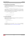
7.2 Defining Custom DOE Strategies . . . . . . . . . . . . . . . . . . . . . . . . . . . . . . . . . . . . . . . . . . . . . . . . . . . . . . . 231
7.2.1 Running the Script . . . . . . . . . . . . . . . . . . . . . . . . . . . . . . . . . . . . . . . . . . . . . . . . . . . . . . . . . . . . . . . . . 232
7.2.2 Compiling the Script . . . . . . . . . . . . . . . . . . . . . . . . . . . . . . . . . . . . . . . . . . . . . . . . . . . . . . . . . . . . . . . 232
5
VWF User’s Manual
Table of Contents
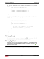
7.2.3 Stopping a Running Script . . . . . . . . . . . . . . . . . . . . . . . . . . . . . . . . . . . . . . . . . . . . . . . . . . . . . . . . . . 233
7.2.4 Loading a Shared Library . . . . . . . . . . . . . . . . . . . . . . . . . . . . . . . . . . . . . . . . . . . . . . . . . . . . . . . . . . . 233
7.2.5 Writing Messages to the Console . . . . . . . . . . . . . . . . . . . . . . . . . . . . . . . . . . . . . . . . . . . . . . . . . . . . . 234
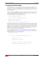
7.3 Defining Target Scripts for Optimization . . . . . . . . . . . . . . . . . . . . . . . . . . . . . . . . . . . . . . . . . . . . . . . . . 235
Chapter 8
Security Concepts in VWF . . . . . . . . . . . . . . . . . . . . . . . . . . . . . . . . . . . . . . . . . . . . . . . .236
8.1 Introduction . . . . . . . . . . . . . . . . . . . . . . . . . . . . . . . . . . . . . . . . . . . . . . . . . . . . . . . . . . . . . . . . . . . . . . . . . 238
8.2 Security Related Dialogs . . . . . . . . . . . . . . . . . . . . . . . . . . . . . . . . . . . . . . . . . . . . . . . . . . . . . . . . . . . . . . 240
Appendix A
Database Maintenance . . . . . . . . . . . . . . . . . . . . . . . . . . . . . . . . . . . . . . . . . . . . . . . . . . 244
A.1 Backing up VWF Data . . . . . . . . . . . . . . . . . . . . . . . . . . . . . . . . . . . . . . . . . . . . . . . . . . . . . . . . . . . . . . . . 245
A.2 vwf_backup. . . . . . . . . . . . . . . . . . . . . . . . . . . . . . . . . . . . . . . . . . . . . . . . . . . . . . . . . . . . . . . . . . . . . . . . . 246
A.2.1 Examples . . . . . . . . . . . . . . . . . . . . . . . . . . . . . . . . . . . . . . . . . . . . . . . . . . . . . . . . . . . . . . . . . . . . . . . 249
A.3 vwf_restore . . . . . . . . . . . . . . . . . . . . . . . . . . . . . . . . . . . . . . . . . . . . . . . . . . . . . . . . . . . . . . . . . . . . . . . . . 252
A.4 SRDB Utility . . . . . . . . . . . . . . . . . . . . . . . . . . . . . . . . . . . . . . . . . . . . . . . . . . . . . . . . . . . . . . . . . . . . . . . . 255
A.4.1 Making a Backup . . . . . . . . . . . . . . . . . . . . . . . . . . . . . . . . . . . . . . . . . . . . . . . . . . . . . . . . . . . . . . . . . 255
A.4.2 Restoring a Database from a Backup . . . . . . . . . . . . . . . . . . . . . . . . . . . . . . . . . . . . . . . . . . . . . . . . . . 256
Appendix B
Queuing VWF On The Oracle/SUN Grid Engine/Open Grid Scheduler . . . . . . . . . . . 257
B.1 Installing the Open Grid Scheduler . . . . . . . . . . . . . . . . . . . . . . . . . . . . . . . . . . . . . . . . . . . . . . . . . . . . . 258
B.2 Open Grid Scheduler – Installation with the GUI Installer . . . . . . . . . . . . . . . . . . . . . . . . . . . . . . . . . . . 259
B.2.1 Prerequisites . . . . . . . . . . . . . . . . . . . . . . . . . . . . . . . . . . . . . . . . . . . . . . . . . . . . . . . . . . . . . . . . . . . . . 259
B.2.2 Running the GUI Installer . . . . . . . . . . . . . . . . . . . . . . . . . . . . . . . . . . . . . . . . . . . . . . . . . . . . . . . . . . . 260
B.3 Manuals . . . . . . . . . . . . . . . . . . . . . . . . . . . . . . . . . . . . . . . . . . . . . . . . . . . . . . . . . . . . . . . . . . . . . . . . . . . . 270
B.4 Installation using the Traditional Method . . . . . . . . . . . . . . . . . . . . . . . . . . . . . . . . . . . . . . . . . . . . . . . . 271
B.4.1 Product Manuals . . . . . . . . . . . . . . . . . . . . . . . . . . . . . . . . . . . . . . . . . . . . . . . . . . . . . . . . . . . . . . . . . . 271
B.4.2 Initial Set Up . . . . . . . . . . . . . . . . . . . . . . . . . . . . . . . . . . . . . . . . . . . . . . . . . . . . . . . . . . . . . . . . . . . . . 271
B.4.3 Install the Master Host (qmaster) . . . . . . . . . . . . . . . . . . . . . . . . . . . . . . . . . . . . . . . . . . . . . . . . . . . . . 272
B.4.4 Install the Execution Host (execd) . . . . . . . . . . . . . . . . . . . . . . . . . . . . . . . . . . . . . . . . . . . . . . . . . . . . 281
B.4.5 Install execd on another host . . . . . . . . . . . . . . . . . . . . . . . . . . . . . . . . . . . . . . . . . . . . . . . . . . . . . . . . 285
B.5 Submitting Jobs . . . . . . . . . . . . . . . . . . . . . . . . . . . . . . . . . . . . . . . . . . . . . . . . . . . . . . . . . . . . . . . . . . . . . 287
B.6 Uninstall Open Grid Scheduler . . . . . . . . . . . . . . . . . . . . . . . . . . . . . . . . . . . . . . . . . . . . . . . . . . . . . . . . . 292
B.7 References . . . . . . . . . . . . . . . . . . . . . . . . . . . . . . . . . . . . . . . . . . . . . . . . . . . . . . . . . . . . . . . . . . . . . . . . . 293
Appendix C
Queuing VWF On An LSF Cluster . . . . . . . . . . . . . . . . . . . . . . . . . . . . . . . . . . . . . . . . . 294
C.1 Obtaining and Installing LSF. . . . . . . . . . . . . . . . . . . . . . . . . . . . . . . . . . . . . . . . . . . . . . . . . . . . . . . . . . . 295
C.2 Selecting LSF to be Used . . . . . . . . . . . . . . . . . . . . . . . . . . . . . . . . . . . . . . . . . . . . . . . . . . . . . . . . . . . . . 295
Appendix D
Recommended Practice . . . . . . . . . . . . . . . . . . . . . . . . . . . . . . . . . . . . . . . . . . . . . . . . . 297
D.1 Multi-Threading . . . . . . . . . . . . . . . . . . . . . . . . . . . . . . . . . . . . . . . . . . . . . . . . . . . . . . . . . . . . . . . . . . . . . 298
D.2 Extract Statements. . . . . . . . . . . . . . . . . . . . . . . . . . . . . . . . . . . . . . . . . . . . . . . . . . . . . . . . . . . . . . . . . . . 298
D.2.1 Bad Case (for VWF) . . . . . . . . . . . . . . . . . . . . . . . . . . . . . . . . . . . . . . . . . . . . . . . . . . . . . . . . . . . . . . . 298
D.2.2 Good Case (for VWF) . . . . . . . . . . . . . . . . . . . . . . . . . . . . . . . . . . . . . . . . . . . . . . . . . . . . . . . . . . . . . . 299
D.3 Splitting on line statements in Athena . . . . . . . . . . . . . . . . . . . . . . . . . . . . . . . . . . . . . . . . . . . . . . . . . . . 299
6
VWF User’s Manual
Table of Contents
D.4 Dealing with Error Scenarios . . . . . . . . . . . . . . . . . . . . . . . . . . . . . . . . . . . . . . . . . . . . . . . . . . . . . . . . . . 300
D.4.1 Dealing with Failing Simulations . . . . . . . . . . . . . . . . . . . . . . . . . . . . . . . . . . . . . . . . . . . . . . . . . . . . . . 300
D.4.2 Standard Output and Standard Error . . . . . . . . . . . . . . . . . . . . . . . . . . . . . . . . . . . . . . . . . . . . . . . . . . 300
D.4.3 Extended Job Status Information . . . . . . . . . . . . . . . . . . . . . . . . . . . . . . . . . . . . . . . . . . . . . . . . . . . . . 300
D.4.4 Grid-engine/LSF Jobs Failing . . . . . . . . . . . . . . . . . . . . . . . . . . . . . . . . . . . . . . . . . . . . . . . . . . . . . . . . 300
D.4.5 VWF Background Process not Starting . . . . . . . . . . . . . . . . . . . . . . . . . . . . . . . . . . . . . . . . . . . . . . . . 301
D.4.6 Error Message when Logging into the Database System . . . . . . . . . . . . . . . . . . . . . . . . . . . . . . . . . . 302
D.5 Selecting a Different than the Default Version of a Simulator . . . . . . . . . . . . . . . . . . . . . . . . . . . . . . . . 303
D.6 Splitting on the Simulator Version . . . . . . . . . . . . . . . . . . . . . . . . . . . . . . . . . . . . . . . . . . . . . . . . . . . . . . 304
D.7 Splitting on the Init line of Athena . . . . . . . . . . . . . . . . . . . . . . . . . . . . . . . . . . . . . . . . . . . . . . . . . . . . . . 305
7
VWF User’s Manual
Chapter 1
Introduction
What is Virtual Wafer Fab (VWF)
Introduction
1.1 What is Virtual Wafer Fab (VWF)
VWF is designed to be used interactively to mirror procedures performed in real wafer fabs
and to automate the user-intensive tasks of preparing experiments, running simulations, and
analyzing results. This results in a convenient use of process and device simulation tools both
in two and three dimensions and the ability to perform large, simulation-based design studies.
1.1.1 Advantages
VWF provides major advantages:
•
•
Greatly reduces the cost of experimentation because you only need this software to
perform them.
Greatly reduces the design cycle time because simulations will complete hours or days,
while actual fabrication typically takes weeks or months.
1.1.2 Applications
Here are some of the operations that VWF can perform:
•
•
•
•
•
•
•
•
Studying the effects of process variation on circuit performance
Experimenting layout variation such misalignment and over/under etch on Device
performance
Synthesis and optimization of inductor design
Optimization of circuit performance
Automated calibration
Optimization of Parasitic interconnect versus circuit performance
Inductor PDK generation
SPICE parameter extraction versus process variation
9
VWF User’s Manual
Features
Introduction
1.2 Features
VWF helps you perform design experimentation efficiently without resorting to third party
software. Some of the advanced features provided are described below.
1.2.1 Database
The heart of the VWF system is a structured multi-user database that contains all of the data
associated with the design process. The software uses a modern, scalable, SQL-92 based
database engine to ensure integrity of your data.
In addition to the SQL-92 database engine, large binary files as generated by simulators are
stored in the file system in a central location. All files pertaining to a particular experiment
can be browsed, manipulated, and retrieved for visualization by the VWF software.
1.2.2 User-Friendly
Access to or control of the data is provided through comprehensive Graphical User Interface
(GUI) technology. It is not required for you to learn any computer specific command syntax
or require the use of any other software beyond that provided by VWF.
The results are automatically presented in the form of spreadsheets and graphical charts that
require little or no user interaction to extract the desired information.
VWF offers a mechanism to extend the built-in experimental design models. A modern
scripting language is offered to implement your own design model.
1.2.3 Experimental Design
The amount of simulations required to cover all possible variations in input values is
immense. Modern experimental designs are used to generate combinations of Input
Parameters that help maximize the amount of information obtained from a given number of
simulations.
VWF generates Split Lot Parameter Values for many of the commonly used experimental
design models, including Full and Partial Factorial, Box-Behnken, Composite, and Latin
Hypercube.
1.2.4 Optimization
VWF allows you to carry out experiments, where a chosen optimization algorithm is used to
vary split parameters so that a defined target is minimized. This allows you to use VWF for
automated calibration tasks and to optimize process parameters in a process simulation.
Supported optimization algorithms are Levenberg-Marquardt, Genetic Algorithm, and
Simulated Annealing to name a few.
1.2.5 Network Execution
A queuing and scheduling system automatically submits simulations for execution on remote
machines if they are available. This permits the computing load to be spread across any
number of machines on a network. The software supports standardized modern grid
computing facilities like Open Grid Scheduler (OGS) or Load Sharing Facility (LSF).
10
VWF User’s Manual
Features
Introduction
1.2.6 Security Features
VWF supports advanced security features. For security sensitive applications, all data can be
held on a central VWF server. It is possible to define privileges such as read, write, or execute
on a per user level. Groups can be defined to implement department security profiles. User
authentication on the network follows the SASL (Simple Authentication and Security Layer)
standard.
1.2.7 Scripting Interface
VWF supports a powerful scripting interface to run JavaScript scripts. In addition to creating
your own experimental designs, this can be used to run VWF experiments without the need of
the GUI (batch mode).
11
VWF User’s Manual
Simulators
Introduction
1.3 Simulators
VWF supports 2D and 3D process and device simulators, SPICE parameter extraction and
circuit simulators as well as interconnect parasitic extraction tools.
12
VWF User’s Manual
Chapter 2
Installation
VWF Variants
Installation
2.1 VWF Variants
The VWF software can be utilized in several ways. Depending on how you use VWF,
different installation steps are required. The following shows a brief outline of the different
ways of using VWF. This is followed by detailed installation instructions.
Depending on what features of VWF you would like to use, there are four ways you can use
VWF:
•
File mode - This does not utilize a database at all. Instead, the necessary information to
run experiments is kept in files.
•
Database mode - A database is utilized to store experiments and results. Execution of
experiments takes place either on your local workstation or on a central VWF server.
Advanced security strategies are enforced.
Open Grid Scheduler (OGS) queue - Allows you to utilize an Open Grid Scheduler
cluster to run simulations.
Load Sharing Facility (LSF) queue - Allows you to utilize an LSF cluster to run
simulations.
•
•
All four variants require you to at least install the VWF TAR file. This step is explained in
the next section.
14
VWF User’s Manual
Installing the VWF TAR file
Installation
2.2 Installing the VWF TAR file
The VWF software is shipped as a single TAR file, which contains all components of VWF.
This TAR file must be untarred in a directory, which is accessible from all machines you
would like to run the VWF software from. A suitable location for this is an NFS drive on a
dedicated file server. This drive must be mounted on every workstation, which will be able to
run the software.
Note: If you plan to also install the database system, then the database must be running on the very same
machine where you untar this VWF TAR package. If you want to install the database on a separate machine,
you will have to download and install an extra TAR package. Please contact a Silvaco representative for
further details.
Note: You can safely untar this package over a previously created Silvaco installation. All packages are versioned
so that you can later continue to use the previously installed software even after the untar operation has
finished. In case you want to revert to the state before installation of this package, you need to copy the
whole install tree into a separate location before you start the untar.
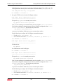
In the following example, the contents of the VWF TAR file are untarred into the /build/
silvaco directory:
[root@lannach root]# cd /build/
[root@lannach build]# mkdir silvaco
[root@lannach build]# cd silvaco
[root@lannach silvaco]# tar xvzf 12113-vwf-2010-00-rh64.tar.gz
bin/acroread
bin/dbinternal
bin/deckbuild
bin/ghostprint
bin/vwf
bin/maskviews
bin/sedit
bin/sflm
bin/sflm_access
bin/sflm_monitord
bin/showid
bin/sipc
bin/gbak
bin/gsec
bin/isql
bin/fbguard
bin/fbmgr
15
VWF User’s Manual
Installing the VWF TAR file
Installation
bin/firebird
bin/smd5sum
bin/srdb
bin/vwf_server
bin/vwf_upgrade
bin/vwf_backup
bin/vwf_restore
bin/spayn
bin/sencrypt
.
.
.
The output of the tar command was truncated. Many more files as shown here will be
displayed on the screen.
16
VWF User’s Manual
VWF Modes
Installation
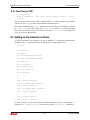
2.3 VWF Modes
2.3.1 File Mode
This is the simplest way of running VWF. A big advantage of this mode is that no extra
installation steps are necessary. A disadvantage of this mode, however, is that sharing data
with other users of your department or company may become slightly more difficult as you
need to put the files in a shared location.
You can invoke vwf in file mode using:
vwf -filemode
Note: You have to run every experiment in its own directory. This is because the VWF file mode creates (and
removes) uniquely named sub-directories whenever the experiment is started or restarted.
2.3.2 Database Mode
This is the standard mode. It is invoked if you start vwf without the -filemode option. VWF
keeps all experiment related data in a database system and all simulation files in a central
directory. VWF is directly built upon a 64-bit relational database system called Firebird to
store experiment data. This data includes all the statically entered data as described in Chapter
3 “Using the VWF GUI”, plus the information that is computed during runtime of an
experiment. These are the results extracted from simulations. Firebird, originally developed
by Borland, is freely available from The Firebird Project.
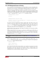
To utilize this mode, you need to first install the Firebird relational database system. Next,
you need to create a specific VWF database in Firebird. This setup will then allow you
running simulation jobs directly on your local workstation or on a grid computing
environment. One notable difference to filemode is also that experiments are executing in the
background. This allows you to close the GUI after the experiment was started. In the
simplest case, the background execution takes place on the very same machine where you
also run the GUI from.
The default configuration in this mode is to store all simulation result files relative to your
UNIX home directory. The full directory of an experiment is as follows:
$HOME/vvwf_basedir/<username>/<database_name>/<experiment_name>_10001/
where
•
•
•
•
$HOME is your home directory,
username is the name of your UNIX account,
database_name is the name of the database, which was given when it was created using
the SRDB utility, and
experiment_name is the name of the experiment in VWF.
The trailing number (_10001) is an automatically chosen sequence number to avoid name
clashes.
The first part of the directory ($HOME/vwf_basedir) can be configured to point into a
different location using the VWF_BASEDIR environment variable.
17
VWF User’s Manual
VWF Modes
Installation
Note: You do not need to change the location of the simulation files unless you want to use either LSF or the
Open-Grid-Scheduler (OGS) queuing system.
OGS and LSF will require a location, which is accessible from all machines that are part of
the grid.
The VWF background process (vwf_server) will log information to a log file. While not
normally concerned with log files, they can be helpful in case there is an error condition. The
location of the log file defaults to $HOME/vwf_logs. It can be changed by using the
VWF_LOGDIR environment variable.
When any of the VWF_BASEDIR or VWF_LOGDIR variables are changed, please make sure the
change is propagated to all components of VWF. To do so, please set these variables directly
in your .cshrc or .bash_profile startup files, terminate all components of VWF including
the vwf_daemon, and completely log out of your account. After logging back in and restarting the VWF, it will indicate that the vwf_daemon is being started again as soon you
connect to a database.
As an advanced configuration option, you can decide to run the VWF background processes
completely isolated on a separate server machine. This makes sense for instance if your
workstation is no LSF or OGS submit host. It also helps you to share data between several
users as all data are kept on a central server location. Finally, it also allows you to implement
a more tight security policy, as simulation files are no longer directly accessible from regular
UNIX accounts. No NFS access is needed from the VWF GUI to the server machine. Please
proceed directly to “Database Mode – Installing the vwf_daemon on a central VWF server”
on page 28 below.
Upgrading from a Previous VWF Install
If you are upgrading from a previous release, it may be necessary to manually stop the
vwf_daemon after the upgrade. This is because the vwf_daemon runs in the background and
is not normally stopped when you terminate VWF. Stopping of the vwf_daemon is only
necessary, however, in case a new vwf_daemon version was installed by the upgrade.
If you are upgrading from a 2.10.xx, 2.8.xx, 2.6.xx , 2.4.xx, or 2.2.xx version of VWF, then
you need to upgrade the database to version 7 (v7). Upgrading a database is done by using the
SRDB utility.
Note: Version numbers for databases evolve in a different numbering scheme as do version numbers for the VWF
software. Versions 2.10.0 to 2.10.3 of VWF were based on the version 5 (v5) database schema. 2.10.xx
versions of VWF above 2.10.3 use the database schema version 6 (v6). The 2.12.xx series of VWF uses
database schema version 7 (v7).
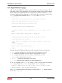
Note: It is advisable to fully backup your existing database before you do the actual upgrade.
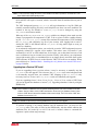
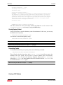
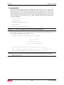
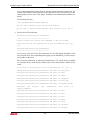
To perform a backup of an existing database and all simulation files, you must use the
vwf_backup utility. This utility is based on the SRDB utility with the notable addition that
simulation files are backed up as well. If the tool is invoked without a command-line
argument, it prints a short usage message:
18
VWF User’s Manual
VWF Modes
Installation
V W F _ B A C K U P
Copyright (C) 1984 - 2013
Silvaco Inc. All rights reserved
ERROR 2013-03-14 09:38:43,749 option -host missing
ERROR 2013-03-14 09:38:43,749 option -passwd missing
ERROR 2013-03-14 09:38:43,749 option -db missing
ERROR 2013-03-14 09:38:43,749 option -file missing
usage: vwf_backup -host hostname -db database-name -passwd password
-file output file [-srdb path_to_srdb] [-flags flags_to_srdb]
[-properties properties-file][-bd base_directory]
-srdb
... select which srdb version to use (default uses srdb from $SILVACO/
bin)
-flags ... pass flags to srdb command (e.g. to select a particular version)
-properties ... take all options from a properties file (all other options are
ignored)
e.g. : vwf_backup -host lannach -db vwf_test -passwd simucad
-file backup_test_20081210.tgz
This will attempt to make a backup of database vwf_test
on server lannach and store the dump together with all
result files in a file called backup_test_20081210.tgz.
The password used for the connection is simucad.
or
: vwf_backup -srdb /build/silvaco/bin/srdb -flags "-V 10.0.11.R"
-host lannach -db vwf_test -passwd simucad
-file backup_test_20081210.tgz
Same as above except that srdb is taken from /build/silvaco/bin
rather than from $SILVACO/bin, and that version 10.0.11.R is executed
instead of the default version.
or
: vwf_backup -properties properties.config
This will take all options from the properties file
instead of the commandline
19
VWF User’s Manual
VWF Modes
Installation
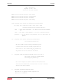
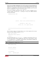
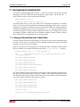
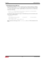
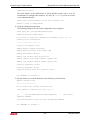
Below an example of how a database called vwf_demo2 can be backed up into a file called
vwf_demo2.tgz.
[root@lannachn ~]# vwf_backup -host lannachn -passwd simucad -db vwf_demo2
-file vwf_demo2.tgz
V W F _ B A C K U P
Copyright (C) 1984 - 2013
Silvaco Inc. All rights reserved
INFO
version info:vwf_backup 2.12.0.R (Thu Mar 14 15:32:53 CET 2013)
INFO Backing up simulation files from directory "/build/silvaco/var/
vwf_base_local/vwf_demo2" to file:vwf_demo2.tgz
The runtime output indicates that the backup succeeded.
Both the simulation result files and the database dump are put into the file named
vwf_demo2.tgz.
The created file (vwf_demo2.tgz) can later be used to restore the database and all created
simulation files. This will be important in case something goes wrong during the upgrade
process.
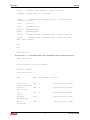
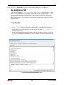
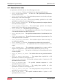
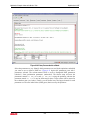
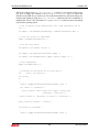
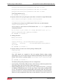
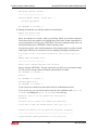
After creating a backup, invoke the SRDB utility and run the upgrade script as shown in the
example below.
thomasb@lannachn$ srdb
S R D B
Version:
srdb 2.4.22.R (2013-03-15T15:29:08)
Copyright (c) 1984 - 2013
Silvaco, Inc.
All rights reserved
======================================================
SRDB >login lannachn
Password for server lannachn :
SRDB lannachn >upgrade vwf_demo2 VWF 6 7
LIBRARIES /build/silvaco/lib/firebird/1.5.2.R/x86_64-linux/lib:/build/silvaco/lib/
firebird/1.5.2.R/x86_64-linux:/build/grid/lsf/7.0/linux2.6-glibc2.3-x86_64/lib:/
usr/lib:/lib:/usr/openwin/lib:/build/silvaco/lib/support/x86_64-linux:/build/silvaco/lib/support/i386-linux
Use CONNECT or CREATE DATABASE to specify a database
Database vwf_demo2 type VWF upgraded from version 6 to 7 on server lannachn.
SRDB lannachn >
20
VWF User’s Manual
VWF Modes
Installation
The last line of the runtime output of this example indicates that the upgrade was successful.
The database can now be accessed by VWF version 2.12.0 or greater only. It is no longer
possible to open the database using an older version of VWF. There is also no way of
downgrading a previously upgraded database. If you want to access the data using an older
version of VWF, you must use the VWF version, which actually corresponds to the database
schema. If there is an error during an upgrade and you want to go back, use the vwf_restore
utility to restore the state of the database to when you first ran the upgrade. Please note that–
as a safety measure–the restore utility does not overwrite any existing data in your system.
Therefore, you must manually remove both the database (using SRDB) and the simulation
files before a restore will succeed.
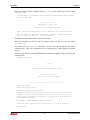
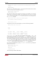
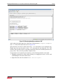
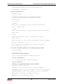
Below, the output of the SRDB utility is shown for the case where you need to upgrade your
system over several schema versions. As an example, a database called vwf_v2 is upgraded
from version 2 to version 7:
SRDB lannachn >upgrade vwf_v2 VWF 2 7
LIBRARIES /build/silvaco/lib/firebird/1.5.2.R/x86_64-linux/lib:/build/silvaco/lib/
firebird/1.5.2.R/x86_64-linux:/build/grid/lsf/7.0/linux2.6-glibc2.3-x86_64/lib:/
usr/lib:/lib:/usr/openwin/lib:/build/silvaco/lib/support/x86_64-linux:/build/silvaco/lib/support/i386-linux
Use CONNECT or CREATE DATABASE to specify a database
KEY_OUT ERR_OUT
===================== ================
6071 <null>
USERKEY ERROR
===================== ======
-1 USEDN
LIBRARIES /build/silvaco/lib/firebird/1.5.2.R/x86_64-linux/lib:/build/silvaco/lib/
firebird/1.5.2.R/x86_64-linux:/build/grid/lsf/7.0/linux2.6-glibc2.3-x86_64/lib:/
usr/lib:/lib:/usr/openwin/lib:/build/silvaco/lib/support/x86_64-linux:/build/silvaco/lib/support/i386-linux
Use CONNECT or CREATE DATABASE to specify a database
21
VWF User’s Manual
VWF Modes
Installation
LIBRARIES /build/silvaco/lib/firebird/1.5.2.R/x86_64-linux/lib:/build/silvaco/lib/
firebird/1.5.2.R/x86_64-linux:/build/grid/lsf/7.0/linux2.6-glibc2.3-x86_64/lib:/
usr/lib:/lib:/usr/openwin/lib:/build/silvaco/lib/support/x86_64-linux:/build/silvaco/lib/support/i386-linux
Use CONNECT or CREATE DATABASE to specify a database
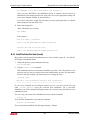
Database vwf_v2 type VWF upgraded from version 2 to 7 on server lannachn.
SRDB lannachn >
Please note the last line, which indicates that the database was properly upgraded from
version 2 to version 7.
Installing the Firebird Database System
This is the default mode of operation where all your simulation jobs are run on your local
workstation. You will need to install firebird when you want to run VWF in database mode.
Note: If you already have installed firebird with a different Silvaco software package (e.g., Utmost IV), then you do
not need to redo this step. Please proceed directly to “Creating a VWF Database” on page 23.
Note: All firebird (not SRDB) commands described in this manual need to be run as root or they will fail.
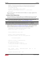
Firebird has been copied onto your hard disk when you untarred the VWF software from the
VWF tar package (see Section 2.2 “Installing the VWF TAR file”). After the files have been
untarred, you must install firebird. To do this, invoke the firebird script as follows:
[root@lannach ~]# /build/silvaco/bin/firebird -install
Running s_install version: 2.0.3.R
please wait...
Currently 921944 KB free in /tmp (>= 8000)
Preparing to install the Firebird Database Server.
This procedure will modify or create the following system files:
/etc/rc.d/init.d/firebird
Backups will be created in /var/tmp/s_install.bak
before any files are modified.
Run '/build/silvaco/etc/s_install -rm-bak' or
'/var/tmp/s_install.bak/remove' to remove backup files.
Do you wish to proceed? [y|n] y
Using
database
location
lannach.Silvaco.com (10.72.5.1)
/build/silvaco/var/srdb
owned
by
host
Configuring /build/silvaco/var/srdb ... done.
22
VWF User’s Manual
VWF Modes
Installation
Verifying permissions ... done.
Installing servers in init.d ...
Installation done.
Starting and verifying servers ...
LIBRARIES
/build/silvaco/lib/firebird/1.5.2.R/x86_64-linux/lib:/build/silvaco/
lib/firebird/1.5.2.R/x86_64-linux:/build/silvaco/lib/firebird/1.5.2.R/x86_64linux/lib:/build/silvaco/lib/firebird/1.5.2.R/x86_64-linux:/usr/lib:/lib:/usr/
openwin/lib:/build/silvaco/lib/support/x86_64-linux:/build/silvaco/lib/support/
i386-linux:/usr/lib:/lib:/usr/openwin/lib:/build/silvaco/lib/support/x86_64linux:/build/silvaco/lib/support/i386-linux
Verification done.
FIREBIRD installation completed successfully.
After that, firebird has been successfully installed and databases can be created in the
/build/silvaco/var/srdb directory by using the SRDB utility.
Starting/Stopping Firebird
It may be necessary to stop the database system for maintenance. In this case, you can stop
the firebird server by using:
/build/silvaco/bin/firebird -stop
You can later re-start firebird again by using:
/build/silvaco/bin/firebird -start
Note: Firebird is stopped and started automatically whenever you reboot your system.
Note: Starting and stopping the firebird server requires root privileges.
De-Installing Firebird
To de-install firebird from your system, please use the following command:
/build/silvaco/bin/firebird -deinstall
This will undo what has been done with firebird -install but will not remove the
databases from your system. You will have to remove database files from directory
$SILVACO/var/srdb or remove the directory altogether. When you do a -deinstall
followed by a -install, the same databases that were available before the -deinstall will
be available after the -install again.
Note: Uninstalling the firebird server requires root privileges.
Creating a VWF Database
23
VWF User’s Manual
VWF Modes
Installation
Some system and database administration work will be required to setup and maintain the
database system for VWF. VWF databases can coexist with Utmost IV databases on the same
firebird server. You do need to create at least one separate VWF database. To create a VWF
database, use the SRDB utility. The following gives a short description of how to use this
utility. See the SRDB User’s Manual for more information.
First, invoke the SRDB command-line utility. Make sure you have an SRDB version of
2.4.22.R or higher. You don't need root privileges to run any of the SRDB commands
described in this manual.
thomasb@lannachn$ srdb
S R D B
Version:
srdb 2.4.22.R (2013-03-15T15:33:57)
Copyright (c) 1984 - 2013
Silvaco, Inc.
All rights reserved
======================================================
SRDB >
Next, you need to connect to a running database server. In this example, this is the same
machine from where SRDB is invoked (lannachn):
SRDB >login lannachn
Password for server lannachn :
lannachn >
The prompt changes from SRDB > to lannachn > to indicate a successful login. There is an
interactive help available within the SRDB utility, which can be invoked anytime by typing
help. The output of the help command is context sensitive. It also depends on whether you
are logged into a server or connected to a database.
Note: The default password for a database server is simucad.
SRDB lannachn >help
Available Commands
==================
list databases
connect
<database_name>
24
VWF User’s Manual
VWF Modes
backup
Installation
<database_name> <backup_file_name> [overwrite]
backup_all <target_directory> [overwrite]
create
<database_name> <database_type> [<target_directory>
[<database_version>] ]
create
accutools
delete
<database_name>
disable
<database_name>
enable
<database_name>
restore
<backup_file_name> <database_name> [<target_directory>]
upgrade
<database_name> <database_type> <old_version_number>
<new_version_number>
exit
quit
SRDB lannachn >
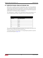
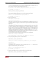
You can use the list command to obtain a list of all databases already existing on the server:
SRDB lannachn >list
You are logged in to server lannachn.
Available Databases
===================
Name
Type
baseline_2012
baseline_2012.fdb
VWF
4
/build/silvaco/var/srdb/
tutorial
tutorial.fdb
VWF
4
/build/silvaco/var/srdb/
vwf
vwf.fdb
VWF
6
/build/silvaco/var/srdb/
vwf_demo2
vwf_demo2.fdb
VWF
7
/build/silvaco/var/srdb/
vwf_v2
vwf_v2.fdb
VWF
Version Number
7
Location
/build/silvaco/var/srdb/
25
VWF User’s Manual
VWF Modes
Installation
vwf_v5
vwf_v5.fdb
VWF
5
/build/silvaco/var/srdb/
vwf_v5_up
vwf_v5_up.fdb
VWF
6
/build/silvaco/var/srdb/
vwf_v5_upgraded
VWF
vwf_v5_upgraded.fdb
6
/build/silvaco/var/srdb/
vwf_v6
vwf_v6.fdb
VWF
6
/build/silvaco/var/srdb/
vwf_v6_test
vwf_v6_test.fdb
VWF
6
/build/silvaco/var/srdb/
vwf_v6_tpb
vwf_v6_tpb.fdb
VWF
6
/build/silvaco/var/srdb/
vwf_v6_upgraded
VWF
vwf_v6_upgraded.fdb
7
/build/silvaco/var/srdb/
SRDB lannachn >
To delete a database, use the following command:
SRDB lannachn >delete vwf
LIBRARIES
/build/silvaco/lib/firebird/1.5.2.R/x86_64-linux/lib:/
build/silvaco/lib/firebird/1.5.2.R/x86_64-linux:/build/grid/lsf/
7.0/linux2.6-glibc2.3-x86_64/lib:/usr/lib:/lib:/usr/openwin/lib:/
build/silvaco/lib/support/x86_64-linux:/build/silvaco/lib/support/
i386-linux
Use CONNECT or CREATE DATABASE to specify a database
Database vwf deleted from server lannachn.
SRDB lannachn >
To create a new VWF database, use:
SRDB lannachn >create vwf VWF /build/silvaco/var/srdb
Database creation. Database version not specified. Defaulting to 7.
LIBRARIES
/build/silvaco/lib/firebird/1.5.2.R/x86_64-linux/lib:/
build/silvaco/lib/firebird/1.5.2.R/x86_64-linux:/build/grid/lsf/
7.0/linux2.6-glibc2.3-x86_64/lib:/usr/lib:/lib:/usr/openwin/lib:/
build/silvaco/lib/support/x86_64-linux:/build/silvaco/lib/support/
i386-linux
Use CONNECT or CREATE DATABASE to specify a database
KEY_OUT ERR_OUT
===================== ================
6071 <null>
26
VWF User’s Manual
VWF Modes
Installation
Database vwf created as /build/silvaco/var/srdb/vwf.fdb on server
lannachn.
SRDB lannachn >
This will create a VWF database named vwf. The output should be similar to the one shown
above. Now, connect to the new database as follows:
SRDB lannachn >connect vwf
SRDB lannachn [vwf] >
The prompt will change again to indicate the connection to the database was successful.
Finally, create a user in the new database. The command below will create a user called
thomasb with a password called thomasb. Note that the password is the second argument to
the create user command.
SRDB lannachn [vwf] >create user thomasb thomasb
User thomasb created successfully.
SRDB lannachn [vwf] >
To print the list of active users on this database, you can use the following command:
SRDB lannachn [vwf] >list users
Users
=====
User Name : admin
Status : NORMAL
Groups :
User Name : superuser Status : SUPERUSER Groups :
User Name : thomasb
Status : NORMAL
Groups :
SRDB lannachn [vwf] >Here, three users are displayed. The first entry – admin – was
created when the VWF database was created using the create command above. This user is
the VWF administrator and can be used to modify the security settings for all objects in the
VWF database independent from their ownership. The second user is the SRDB internal
superuser. This is not a VWF specific user. It does not have any function in the VWF
system. Please consult the SRDB manual for more details on that user. Finally, the third user
– thomasb – is the one that was created using the create user command above.
Now, terminate the SRDB utility by typing quit or use exit several times to go through the
different connection levels.
SRDB lannachn [vwf] >exit
SRDB lannachn >exit
SRDB >quit
thomasb@lannachn$
You are now ready to start the VWF software.
27
VWF User’s Manual
VWF Modes
Installation
In database mode, you can actually close the VWF while experiments are running. When you
start an experiment, VWF starts a background job for you, which will take care of executing
the experiment.
Database Mode – Installing the vwf_daemon on a central VWF server
You can opt to run all experiments on a central VWF server. This allows you to completely
separate the VWF GUI from the VWF job execution module. This enables you to utilize an
Open Grid Scheduler or LSF cluster when your workstation does not have direct access to the
grid (is no submit host). This mode also does not store the simulation result files on your
workstation but keeps all files on the central server instead. No access to server directories
(e.g., using NFS) is necessary from your workstation in this mode.
The server side is completely separated from the GUI, which will normally run on a different
workstation and which can be closed after an experiment was started. As soon an experiment
is started, processes are created on the server and on the available grid computing
environment. These processes run under a configured user id. A regular VWF user does not
need UNIX rights to access data owned by that user. Instead, control over all data both
database as well as files (simulation results) is controlled solely by the VWF security system.
Server processes are created (and killed) by the vwf_daemon process, which must be installed
prior to running VWF.
To install the vwf_daemon, you need to run "vwf -install". This will prompt for the user
ID to use as well as for a directory to store the simulation result files. It is suggested to create
a separate user (e.g., vwf_user) for that purpose. The user must be available on all machines,
which are part of the cluster environment, but not necessarily on the user's workstation that is
used to run the GUI.
The command "vwf -install" will also install the firebird database system. Therefore, a
separate "firebird -install" is not necessary if the vwf_daemon is being installed.
Note: In your VWF preferences, you have to change the execution host from the default ("localhost") to
match the central server.
Note: If the firebird system has already been installed previously, then it is not installed again by this step.
2.3.3 Single Machine Queue Mode
This mode allows you to run simulation jobs on the machine, which also runs the VWF
software (i.e., the machine where you started vwf) and is the default queuing mode. It can be
28
VWF User’s Manual
VWF Modes
Installation
used both in file mode and in database mode. The queue mode is defined in the preferences
panel of the VWF software. The single machine queue offers three options to configure. The
first option is the maximum number of jobs, which can execute at the same time. The second
option is a load limit, which defines a maximum load, which should not be exceeded (Figure
4-14). The load limit is useful when the machine is also used to run jobs outside VWF. In this
case, externally run jobs will increase the load limit of the system, which results in less jobs
being started from VWF. Finally, the third option is the nice increment level. All processes
started by the local queue will have their nice level incremented by the value given in this
setting.
Note: When you start jobs outside VWF, it will take a while until the configured load limit will be noticeable. This
is because VWF does not actively terminate running jobs if a limit is exceeded but avoids starting new jobs
instead. The same is true if you change the load limit during runtime.
2.3.4 DRMAA mode
This mode allows you to run simulation jobs on a cluster of workstations. DRMAA stands for
Distributed Resource Management Application API and defines a standard to interface a grid
computing facility. The DRMAA queuing system can be used both in file mode and in
database mode. You must select this mode if you want to utilize a grid computing
environment.
This version of VWF supports two flavors of cluster systems. One is the open source product
Open Grid Scheduler (OGS), and the other is the commercially available Load Sharing
Facility (LSF).
Note: There is a history of open source grid software supported from VWF. The formerly open source package
called Sun Grid Engine is no longer in the open source. Instead, a commercial product called Oracle Grid
Engine (OGE), which is based on the Sun Grid Engine is available from Oracle. Additionally, there is the
Open Grid Scheduler, which is also based on Sun Grid Engine but is available in the open source.
Note: VWF supports all three flavors: the original 6.2u5 version of Sun Grid Engine, the newer Oracle Grid Engine,
and the Open Grid Scheduler.
The VWF tar package contains a version of the Open Grid Scheduler. This is available from
the common sub directory of VWF. Please consult the installation instructions given in the
Appendix B “Queuing VWF On The Oracle/SUN Grid Engine/ Open Grid Scheduler” on
how to install an Open Grid Scheduler cluster system.
29
VWF User’s Manual
Chapter 3
Using the VWF GUI
Overview
Using the VWF GUI
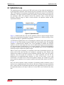
3.1 Overview
This chapter gives an overview of the Graphical User Interface (GUI) components of the
VWF software. All components are explained by means of screen-shots and descriptions. The
screen-shots were prepared on the Linux operating system and the KDE window manager.
31
VWF User’s Manual
Examples Shipped with VWF
Using the VWF GUI
3.2 Examples Shipped with VWF
VWF comes with a set of examples for you to browse. Depending on the mode of operation,
there are three ways you can access these examples. The first method uses the vwf_restore
command to create a whole database containing (only) the examples and a user called demo.
The second method allows you to load the examples into an existing database. The third
method allows you to open examples individually in filemode. Please note that in order to
keep the examples small and loading times short, they do not contain any result files.
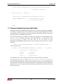
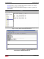
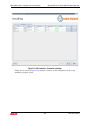
3.2.1 Creating the vwf_examples Database
To create the database, please issue the following command:
vwf_restore -host lannach -passwd simucad vwf_examples.tgz
This command will create a database called vwf_examples, which contains a single user
called demo (password demo). When connected to this database (see below for a description
of how to do this), you will find a single directory called examples, which contains the
shipped examples.
The command may issue a warning as follows about the base directory having changed:
Changing experiment base directories of imported DB from:/build/
silvaco/var/vwf_base/vwf_examples to:/site/alpha/var/vwf_base
vwf_examples
The warning indicates that the base directory at the time the file was created is different from
the base directory on your site. You can safely ignore this warning here.
The file vwf_examples.tgz can be found in the examples section of your vwf install tree.
Depending on where you installed vwf, this is typically found at
/build/silvaco/examples/vwf/<version>/vwf_examples.tgz
Please note that this method of loading examples will only succeed on the machine where the
vwf_daemon was installed. If you’re not using the vwf_daemon, use the following method.
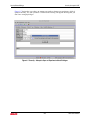
3.2.2 Loading Examples into an Existing Database
You must use the Load Examples menu entry of the Help menu found in the VWF Explorer
window. Please note that this will create a directory called examples in your database. In case
this directory already exists, you must first remove or rename it or you will get an error
message.
3.2.3 Opening Examples in filemode
When you're using filemode, you can choose to directly open an example from the main
dialog that opens after you started VWF using the -filemode option. See Figure 5-53.
32
VWF User’s Manual
Main GUI components
Using the VWF GUI
3.3 Main GUI components
VWF is comprised of the following three main components:
•
•
•
Main Window – This is the first component you are confronted with. You can manage
several databases and open project project from a given database.
The Experiment Editor – This component opens when you edit an existing or create a
new experiment.
The Deck Editor – This is a part of the experiment editor but realized as a separate
application.
The three components will be presented in detail in the following sections.
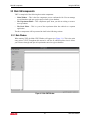
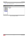
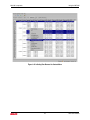
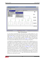
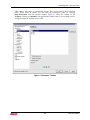
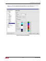
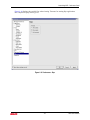
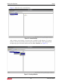
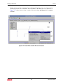
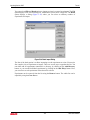
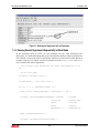
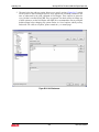
3.3.1 Main Window
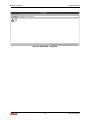
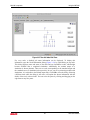
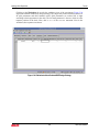
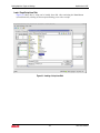
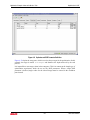
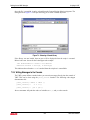
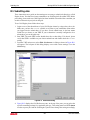
When starting VWF, the Main VWF Window will appear (see Figure 3-1). This is the main
entry point to VWF. Throughout this manual, it will also be called Explorer since it allows
you to browse through and open all experiments stored on a given database.
Figure 3-1 Main VWF Window
33
VWF User’s Manual
Main GUI components
Using the VWF GUI
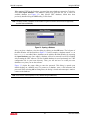
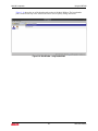
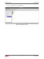
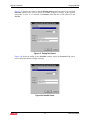
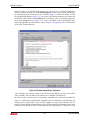
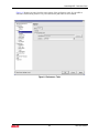
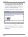
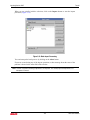
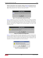
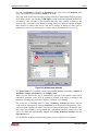
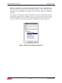
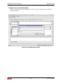
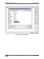
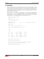
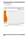
When starting VWF for the first time, you must first open a database connection. To do this,
select FileOpen Database. The Database dialog will open and ask you to select an
available database (see Figure 3-2). Only Silvaco VWF databases, which have been
previously installed using the SRDB utility, will be listed.
Note: An arbitrary number of databases can be installed on a given host and that several hosts are supported by
both VWF and the SRDB utility.
Figure 3-2 Opening a Database
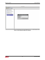
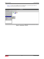
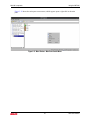
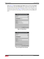
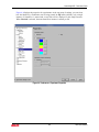
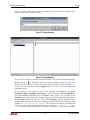
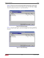
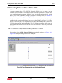
Once you select a database, close the dialog by clicking on the OK button. The left pane of
the Main Window will look similar to Figure 3-3. In this example, a database named vwf on
host localhost was added. More databases can be added to the Main Window by repeating
the Open Database step. Once added, a database will not be removed but will be available
after restarting the VWF software. The list of added databases is stored persistently in a VWF
configuration file in your home directory. Thus, you will not have to re-add your own
databases every time you use the software.
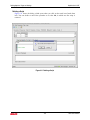
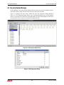
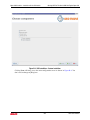
Figure 3-3 depicts the popup dialog to enter the password. This dialog is opened upon
double-clicking on a database entry. To connect to a database, enter a valid username and
password. When selecting OK or hitting Enter, the dialog is closed and an attempt is made to
connect to the database.
Note: Users must be created separately for every database using the SRDB utility.
34
VWF User’s Manual
Main GUI components
Using the VWF GUI
Figure 3-3 Main Window with added VWF Databases
35
VWF User’s Manual
Main GUI components
Using the VWF GUI
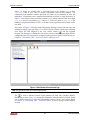
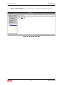
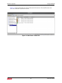
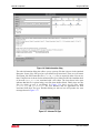
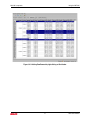
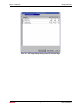
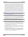
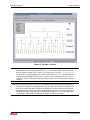
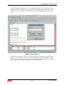
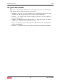
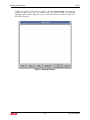
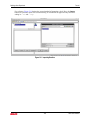
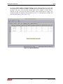
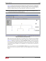
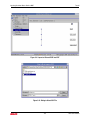
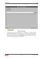
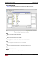
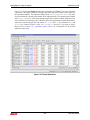
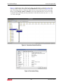
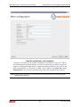
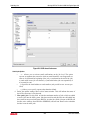
Figure 3-4 shows the scenario after a successful login to the database vwf on host
localhost. VWF is now ready to explore experiments stored in this database. The
connection to the database remains open until you either log out manually or close the
application. Experiments can be organized hierarchically by means of using directories. In
Figure 3-4, the left pane shows a directory named MOSFET, which contains a base deck called
base_deck and two experiments Exp01 and Exp02, which are based on base_deck. The
handling of experiments follows VWF 1.xx in that several experiments can be based on one
base deck.
The bottom of Figure 3-4 displays status information. Starting from the left most entry the
information shown is the user name (demo) followed by the amount of disk space remaining
(Free Space 407.7GB) followed by the “tool version” button ( ) and the copyright
message. The disk space is displayed in red color in case the remaining space drops below a
configurable limit. The limit can be configured in the preferences panel of VWF. Please see
Chapter 4 “Customizing VWF – Preferences Panel” and Figure 4-13.
Figure 3-4 Main Window after successful login
Note: Any given directory may only contain a single base deck.
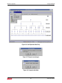
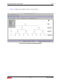
The
is used to indicate selected version numbers for tools like, TonyPlot, SPAYN,
DeckBuild, or others. Figure 3-5 displays the information when the button is clicked. In this
case, a SPAYN version of 2.12.0.R and a DeckBuild version of 4.0.0.C was selected. Please
see Chapter 4 “Customizing VWF – Preferences Panel” on how to change version numbers
for tools.
36
VWF User’s Manual
Main GUI components
Using the VWF GUI
Figure 3-5 Tool Version Information
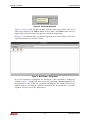
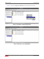
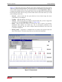
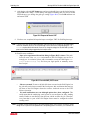
Figures 3-6 and 3-9 show the Main Window with the folders pane hidden. This can be
achieved by clicking on the Folders button of the window. The Folders button acts as a
toggle switch. Thus, the folders will reappear by clicking the button again.
In Figure 3-9, an additional filter was applied to adjust the view of the main pane. Here, only
experiments (but not base decks) are shown.
Figure 3-6 Main Window – hiding folders
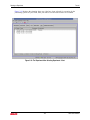
In case an experiment is highlighted, the description of that experiment is displayed if
available. Figure 3-7 displays the main screen with experiment vwfex02 highlighted. The
description pane is only visible if an experiment is highlighted. The contents of the pane are
updated whenever you highlight a different experiment. The description pane is available
regardless of the tree view or any defined filters.
37
VWF User’s Manual
Main GUI components
Using the VWF GUI
Figure 3-7 Main Window – description pane
Figure 3-8 displays the description pane for the case where the folders are hidden (similar to
Figure 3-6 but with an experiment being highlighted).
Figure 3-8 Main Window – description pane (disabled tree view)
38
VWF User’s Manual
Main GUI components
Using the VWF GUI
Figure 3-9 Main Window – using filters
39
VWF User’s Manual
Main GUI components
Using the VWF GUI
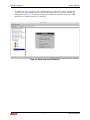
Figure 3-10 shows the use of the breadcrumbs portion of the Main Window. The breadcrumbs
part is located at the top of the window and can be used to quickly change directories.
Figure 3-10 Main Window – using breadcrumbs
40
VWF User’s Manual
Main GUI components
Using the VWF GUI
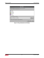
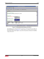
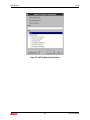
Figure 3-11 shows how the File menu has changed after a successful login. Entries to
manipulate experiments and directories have been added.
Figure 3-11 Main Window – File menu
41
VWF User’s Manual
Main GUI components
Using the VWF GUI
Figure 3-12 shows the Edit menu. This allows you to cut/copy/paste experiments and also to
enter the Preferences dialog.
Figure 3-12 Main Window – Edit menu
42
VWF User’s Manual
Main GUI components
Using the VWF GUI
Figure 3-13 shows the View menu. This allows you to apply filters and switch between the
different available views of the Main Window.
Figure 3-13 Main Window – View menu
43
VWF User’s Manual
Main GUI components
Using the VWF GUI
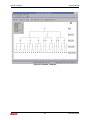
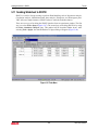
Figure 3-14 shows the List View of the main pane.
Figure 3-14 Main Window – List View
44
VWF User’s Manual
Main GUI components
Using the VWF GUI
Figure 3-15 shows the main pane context menu, which appears upon a right-click in the main
pane.
Figure 3-15 Main Window – Main Pane Context Menu
45
VWF User’s Manual
Main GUI components
Using the VWF GUI
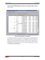
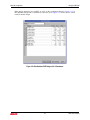
Figure 3-16 shows the Details View. Extra information like the date of last modification or the
user who created the experiment is shown.
Figure 3-16 Main Window – Details View
46
VWF User’s Manual
Main GUI components
Using the VWF GUI
Figure 3-17 shows the Arrange IconsBy Name entry of the main pane context menu.
Figure 3-17 Main Window – Arrange Icons By Name entry
Figure 3-18 Main Window – Icons Arranged By Name
47
VWF User’s Manual
Main GUI components
Using the VWF GUI
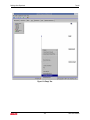
Figure 3-19 shows the menu entry to create a new experiment. To create new experiments,
right click into main pane and select New Experiment.
Figure 3-19 Main Window – New Experiment Menu Entry
48
VWF User’s Manual
Main GUI components
Using the VWF GUI
Figure 3-20 shows the help menu entry. Selecting this menu entry will open the VWF manual.
Figure 3-20 Main Window – VWF Help Menu Entry
49
VWF User’s Manual
Main GUI components
Using the VWF GUI
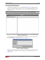
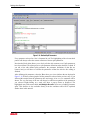
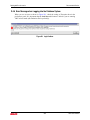
The explorer allows you to move directories from one location to another. To do so, you have
to select the directories to move. This is shown in Figure 3-21. You can select several
directories for movement by holding down the Ctrl key and left-clicking the directories to
move. If you select multiple directories, then the selected directories are rendered in red.
Figure 3-21 Selected Directories for Move
50
VWF User’s Manual
Main GUI components
Using the VWF GUI
To initiate the move operation, press and hold down the left mouse button and drag the
selection to the new location. Once you release the mouse button over the new location, the
dialog shown in Figure 3-22 will open asking you to confirm the operation. If you select OK,
then the move is started otherwise it is canceled.
Figure 3-22 Dialog to Confirm Move Operation
51
VWF User’s Manual
Main GUI components
Using the VWF GUI
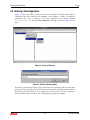
Figure 3-23 shows how the directory tree has changed after the move operation was finished.
In this example, directories named nmos_test1 and nmos_test2 were moved from the root
directory to the directory called MOSFET.
Figure 3-23 Resulting Directory Tree after Move Operation
52
VWF User’s Manual
Main GUI components
Using the VWF GUI
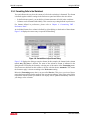
3.3.2 Creating a New Experiment
In order to create a new experiment, you will first need a directory to hold the experiment.
Experiments cannot be stored in the root directory. Once a directory is created, you will then
need to create a baseline. Finally, based on this baseline, you can then create an arbitrary
number of experiments. When experiments are created, the baseline deck is taken as a starting
point. Both the baseline deck as well as the deck in the experiment can be edited
independently from each other. Editing the base deck does not influence the deck of an
experiment and vice versa. Editing the base deck has the effect that all newly created
experiments will be created with the changed baseline.
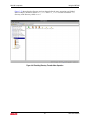
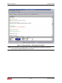
Figure 3-24 shows the dialog to create a new baseline deck. You can choose to either import a
deck from the filesystem, from CVS, or from DeckBuild. Please refer to Chapter 5 “Tutorial”
for a more detailed description of how to import a deck using DeckBuild.
Figure 3-24 Dialog to Create A Baseline Deck
53
VWF User’s Manual
Main GUI components
Using the VWF GUI
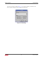
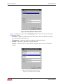
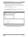
Figure 3-25 depicts how a CVS repository can be accessed. You need to enter host, repository
location, and valid user credentials.
Figure 3-25 CVS Repository Information
54
VWF User’s Manual
Main GUI components
Using the VWF GUI
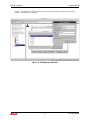
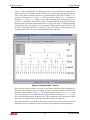
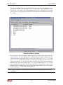
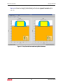
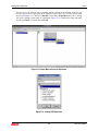
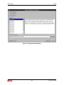
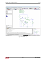
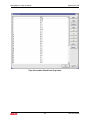
Figure 3-26 shows a populated tree after a successful browse operation. The available content
of the CVS repository is shown. Here, some Athena and Victory examples are shown. In the
right-hand side of Figure 3-26 two files, which have been checked out are shown. The left
pane shows the file anstex01.in from the directory decks/athena/athena_stress.in.
The right pane shows the file vpex01.in from the directory decks/victoryp/vpex01.in.
One of the checked out files can be chosen to become the baseline.
Figure 3-26 Browse View of CVS Repository. Two files have been checked out.
55
VWF User’s Manual
Main GUI components
Using the VWF GUI
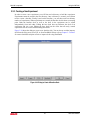
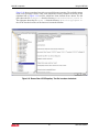
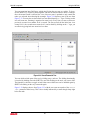
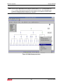
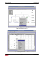
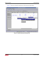
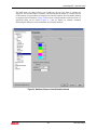
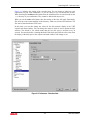
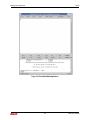
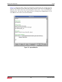
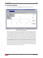
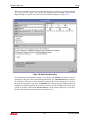
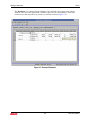
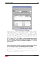
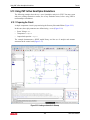
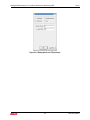
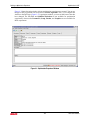
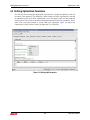
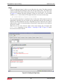
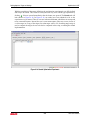
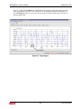
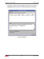
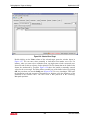
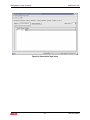
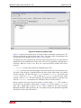
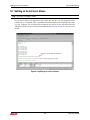
3.3.3 Experiment Editor
Figure 3-27 shows the Experiment Editor. Please refer to Figure 6-3 for the optimization
experiment type. This window appears whenever you create a new experiment or open an
existing one. The editor is used to collect all data necessary to execute an experiment. The
window is composed of several tabs. These are Description, Resources, Deck, Tree,
Worksheet, Jobs, and SplitPlot Worksheet. To open a particular tab, click on the according
label. Figure 3-27 shows the Description tab open. It displays the name of the opened
experiment (vwfex02). The shown example is one of the prepared simulation examples that
are shipped with VWF, which is also available from the Silvaco website.
Figure 3-27 Experiment Editor – Description tab
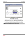
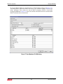
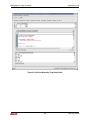
The base directory of an experiment is the top-level directory, which is used for carrying out
simulations with any of the Silvaco simulation tools. A template for this base directory has
been selected during the installation procedure of VWF. When experiments are created, this
template is taken as the prefix for the base directory for the experiment.
Note: In filemode, simulations are run in a sub-directory of the directory where the experiment file is stored.
56
VWF User’s Manual
Main GUI components
Using the VWF GUI
Figure 3-28 depicts how you can manipulate the resources of the VWF experiment. A
resource is a file that is needed when you execute an experiment (run the simulations of the
experiment). Essentially, all files that are mentioned in an input deck are resources. Typical
usage scenarios for resources are mask files, or initialization files for simulators. There are
two possible ways of dealing with resources. They can either be linked from the file system or
they can be stored in the database. Figure 3-28 depicts both variants. The file a.lib is stored
in the database. During the runtime of an experiment, database stored files are copied into the
base directory of the experiment (into a sub-directory called resources) and links to those
files are created from every (sub)directory where a simulation is carried out. In contrast, the
resource called ref.dat is a linked resource, which resides in the directory /tmp/VWF/
Resources. No copy of that file is created, it will directly be linked to from the simulation
sub-directories of the experiment. It is therefore essential for a successful completion of the
simulation that linked resource files are available at the time of experiment execution. The
experiment depends on these external files.
The advantage of database stored resources is that the files are copied (rather than referenced)
on import and do not need to be kept in the original location beyond the import operation.
One of the trade offs between linking and copying is the amount of used disk space. This can
be important if mask files will be reused among various experiments or users. Another aspect
to take into account is that a change in a linked mask is reflected in every experiment, which
uses (links to) that particular mask. It should thus be decided from case to case whether to use
external resources.
Figure 3-28 Experiment Editor – Resources tab
57
VWF User’s Manual
Main GUI components
Using the VWF GUI
Figure 3-29 shows the VWF Deck Editor. This editor allows you to nominate parameters as
split variables. To nominate a parameter right-click on any deck line (as shown in
Figure 3-30) to pop up a list of available parameters of that deck line. Select one of the shown
parameters. By selecting a parameter twice, it is denominated again. A syntax highlighting
scheme is used in the deck, so that a selected parameter can easily be identified in the deck. A
selected parameter is drawn in red. As additional information, the bottom part of this tab
shows a list of all nominated parameters. The syntax highlighting scheme will also draw all
commented deck lines in green.
In this example, the screen shot shows two parameters in the bottom part (time and temp)
and four (different) parameters in the deck pane (called time, temp, dose, and energy). The
bottom pane of the Deck tab also shows block, type, and initial value of the parameter. The
notion of a block is used to group parameters of a single deck line. The block is also visible in
the tree tab and will be shown in another screen-shot.
Figure 3-29 Experiment Editor – Deck tab
58
VWF User’s Manual
Main GUI components
Using the VWF GUI
Figure 3-20 shows the menu that opens when you right-click on a deck line. Here, two
entries, time and temp, of the clicked diffus line are shown as the active parameter. Three
parameters, dryo2, press, and hcl are available as further parameters on this line. Thereby,
the menu entries correspond to the list of active parameters of that line as shown in
Figure 3-29).
Figure 3-30 Experiment Editor – Split Parameter Definition
Right-clicking on any of the parameters in the lower pane of the deck editor reveals a context
menu with two entries (Figure 3-31). Locate will position the cursor in the main deck pane
and within the parameter. Remove will remove the parameter from the list of split
parameters and the coloring will return to that of regular deck text. You can also select Locate
by simply double-clicking on any of the parameter's Value, Block, or Type fields.
59
VWF User’s Manual
Main GUI components
Using the VWF GUI
Figure 3-31 Experiment Editor – Split Parameter Context Menu
Note: Extract statements are recognized whenever a new deck is imported into the experiment or when a new
extract statement is added by editing the deck in the deck tab .
60
VWF User’s Manual
Main GUI components
Using the VWF GUI
You can use the Find Text dialog (Figure 3-32) to search for arbitrary text elements in the
deck. To open the dialog, press Ctrl-F within the deck editor pane.
Figure 3-32 Find Text Dialog
61
VWF User’s Manual
Main GUI components
Using the VWF GUI
Figure 3-33 shows the Tree tab. The Tree tab presents a view at the split tree. Parameters are
grouped in blocks. The split tree results from the set of split parameters and the assigned split
values. In the depicted example, there are two parameter blocks. One block is called diffus.
It consists of parameters time and temp. The other block is called implant. It consists of
parameters dose and energy. Adding or removing a parameter in the deck pane (Figures 329 and 3-30) will directly influence the split tree. The right-hand side of the depicted tree tab
shows a legend with block and parameter names. At the top left, there is a legend explaining
simulation job status and displays a brief job statistic. This legend also shows how the color
of nodes corresponds to the state of a given job. Here, no job has been queued into the job
farming system so far. You can move this legend anywhere in the pane.
Figure 3-33 Experiment Editor – Tree tab
Apart from the coloring scheme, the nodes are also drawn in different shapes depending on
whether several parameters occur at a single deck line. For such parameters, all but the last
parameter a drawn thinner. In Figure 3-33, the split parameter named implant dose is the
first of two parameters on a single deck line. The split parameter named implant energy is
the second and last parameter on this deck line. This is indicated by drawing the node a little
fatter. Only the fat nodes have results and result files available for inspection.
The pane also shows an icon with an arrow and a question mark. You can click on this icon
and then click on any component in the tree pane to get useful help information displayed.
62
VWF User’s Manual
Main GUI components
Using the VWF GUI
You can zoom into large DOE trees, which don't fit into the tree pane as a whole. To do so,
use the SHIFT key of your keyboard together with the left mouse button to draw a rectangle.
Once the mouse button is released, the view of the tree pane is updated to only contain the
nodes you selected when drawing the rectangle. Figure 3-34 depicts a part of the tree from
Figure 3-33. You can also see that a little icon was added showing a “-” sign. Clicking on this
icon will zoom out. Zooming is organized in zoom levels. Every time you start a zoom on a
previously zoomed view another level is created. The first zoom from the initial tree view
creates level 1, the second zoom creates level 2, and so forth. By clicking on the “-” sign, you
are effectively going back one zoom level at a time.
Figure 3-34 View at Zoomed in Tree
You can decide to hide parts of the tree by folding away a sub-tree. The folding functionality
is invoked by holding down the SHIFT key and left-clicking on the node you want to fold.
The function is realized as a toggle switch so that a once folded tree can be unfolded again by
SHIFT left-clicking on the very same node again.
Figure 3-35 displays the tree from Figure 3-33 with the two outer most nodes of the diffus
time parameter folded away. This is also visually indicated by a small triangle shape right
below the node.
63
VWF User’s Manual
Main GUI components
Using the VWF GUI
Figure 3-35 Tree with folded Sub-Trees
For every node, a detailed job status information can be displayed. To display this
information, open the Node Information dialog (Figure 3-36) by right-clicking at any node.
This dialog displays name and status of the node and any simulation results, which might
become available after a completed simulation. Additionally, the runtime output of a
simulation is shown (bottom). There are two tabs corresponding to the standard output and
the standard error of a simulation job respectively. In case you are experiencing troubles with
simulations, it is advisable to check both output tabs. Click OK to close the dialog. Selecting
a different node while the dialog is still active will update the shown information with the
details of the newly selected node. You can resize the panes by clicking and dragging on the
edge between any two panes.
64
VWF User’s Manual
Main GUI components
Using the VWF GUI
Figure 3-36 Node Information dialog
The node information dialog also allows you to open any file that is shown in the Attached
Data pane. Some of the file types have pre-defined tools associated. These are well known
file formats, like 2D/3D structure files (.str) or .log files, as created by Atlas. You can see
that a TonyPlot icon is shown for the mentioned file types. Other files like the simulation deck
of the node (deck-ml.in) are associated with a text editor. The icon shown in the pane
indicates that this file is opened using a text file when double-clicked. Finally, there are also
files for which no tool is pre-defined. In Figure 3-36, there are two files called
picture1.png and picture2.png. The icon indicates that no application has been
associated with these file types. Double-clicking on such an icon will produce the error
message shown in Figure 3-37.
Figure 3-37 Unknown File Type
65
VWF User’s Manual
Main GUI components
Using the VWF GUI
You can associate a command with a file type by right-clicking on the file and selecting Open
With from the menu. A dialog as shown in Figure 3-38 will open. The dialog allows to select
among one of several know types as well as to define a custom type. Here, the utility display
is assigned with files ending in .jpg. If you check the Always use this program to open these
files, then the association is permanently kept in the preferences under the point Registered
Filetypes. If you do not check this box, then the association is lost when you restart VWF. By
clicking Ok, the file picture2.jpg is opened by running the command:
display /tmp/vwf/vwf_basedir/vwf_v7_tpb/exp_10001/jobs/10008 picture2.jpg
Please note the used path as indicated in Figure 3-38.
Figure 3-38 Associating an application with a particular file type
If the file name needs to be in the middle of the command, you can use a placeholder as
shown in Figure 3-39. This will then result in the following command being executed upon
clicking OK.
display /tmp/vwf/vwf_basedir/vwf_v7_tpb/exp_10001/jobs/10008/picture2.jpg
-antialias
66
VWF User’s Manual
Main GUI components
Using the VWF GUI
Figure 3-39 Using a Placeholder for the File Name
67
VWF User’s Manual
Main GUI components
Using the VWF GUI
Figure 3-40 shows the Worksheet tab. The worksheet serves two purposes. First, it is used to
assign split point values to split parameters. Second, it contains all parameters extracted
during simulation.
Figure 3-40 Experiment Editor – Worksheet tab
The worksheet can also be used to remove rows. Figure 3-41 shows a worksheet with several
rows selected for removal. The selected rows are highlighted and the column number is
drawn in brackets ([ ]). In this example, rows 1, 8, 9, 10, and 15 are selected. To select a row,
click on the row header with the left mouse button. To select several rows, hold the Ctrl key
and click on the row header of the row you want to add. Selected rows can be removed by
right-clicking into the worksheet (Figure 3-42) or on the row heading (Figure 3-43) and
selecting Remove selected Branche(s).
68
VWF User’s Manual
Main GUI components
Using the VWF GUI
Figure 3-41 Several Rows Highlighted for Removal
69
VWF User’s Manual
Main GUI components
Using the VWF GUI
Figure 3-42 Initiating Row Removal via Context Menu
70
VWF User’s Manual
Main GUI components
Using the VWF GUI
Figure 3-43 Initiating Row Removal by right-clicking on Row Header
71
VWF User’s Manual
Main GUI components
Using the VWF GUI
3.3.4 Formatting Cells in the Worksheet
You can influence the way how the content of cells in the worksheet is formatted. The format
is defined together with the settings in the Preferences panel and follows the rules below.
•
•
In the Preferences panel, you can define a format common to all cells in the worksheet.
Columns can be formatted individually. This overrules any setting defined in preferences.
For formats defined in preferences, please refer to Chapter 4 “Customizing VWF –
Preferences Panel”.
An individual format for a column is defined by right-clicking on the header of that column.
Figure 3-44 displays the menu entry to open the format dialog.
Figure 3-44 Context Menu to Open Format Dialog
Figure 3-45 displays the dialog to enter the format. In this example, the format for the column
named max_XX_Stress is defined. The name of the column to format is indicated in the
dialog header. You define the format by selecting one of the entries of the Formatting menu.
If no format was defined for this column so far, the selection shows Automatic. This means
the format to apply is chosen according to the Preferences setting.
Below the Formatting menu, there’s an area called Preview. This gives a preview of how a
particular format will look when applied. You can enter an arbitrary value in the value field to
experiment with the format you defined. The display field is updated immediately whenever
you change value or format.
72
VWF User’s Manual
Main GUI components
Using the VWF GUI
Figure 3-45 Define Worksheet Column Format
Figure 3-46 depicts the content of the Formatting pull-down menu. You are presented with
the following choices:
•
•
•
•
Automatic – Applies an automatic format to that column. This is the default if no format
for a column has been selected so far.
Floating point – Formats the number according to the defined precision.
Scientific – Numbers are displayed in scientific notation.
Custom – Allows to define a custom format using the syntax as used in the printf Cfunction.
Figure 3-46 Available Column Formats
73
VWF User’s Manual
Main GUI components
Using the VWF GUI
Figure 3-47 displays the setting in case the Floating point format was chosen. An extra field
Precision appears where you can define the number of digits to display. In the depicted
screen-shot, a value of 6 is selected for Precision. Note that this is also reflected in the
Preview.
Figure 3-47 Floating Point Format
Figure 3-48 shows the dialog for the Scientific notation. Again, the Precision field can be
used to define the number of digits to display.
Figure 3-48 Scientific Format
74
VWF User’s Manual
Main GUI components
Using the VWF GUI
Finally, Figure 3-49 displays the dialog for the Custom format type. Instead of the Precision
field, there is now a field called format string. It allows you to enter a C-type format string.
Please note that the usage of the custom format type is considered an advanced feature. Care
was taken to restrict the format string to floating point formats. An error is displayed in case
an illegal format string is entered. Figure 3-50 displays the situation where an illegal format
string (%s) was entered. The entered format is not accepted in this case and the OK button is
grayed.
Figure 3-49 Custom Format
Figure 3-50 Illegal Format was Entered
75
VWF User’s Manual
Main GUI components
Using the VWF GUI
3.3.5 Defining Splits
There are several ways of entering split points. The most convenient way is to select one of
the predefined DOE designs as shown in Figure 3-51.
The DOE design dialog (Figure 3-51) can be opened by right-clicking on any of the lines in
the worksheet and selecting Design from the context menu. The dialog allows you to select
one of several designs by using the drop down menu. Figure 3-51 shows a 2 Level Full
Factorial with no parameters selected yet. To complete the definition of the DOE design, you
have to select which parameters to use and you have to define the lower and upper bounds for
each selected parameter. After clicking OK, the shown design strategy will insert one node
for the upper and one node for the lower boundary of the selected parameter values. For a
total of n parameters 2n branches are entered into the worksheet. The depicted initial value is
the one that is existing in the deck. By confirming the data with OK, the worksheet is updated
with the new branches.
Adding splits by using a design can be repeated several times in order to add more branches
to the worksheet. The buttons labeled Replace Existing and Add to existing allow you to
decide whether a worksheet will be overwritten with the new design or whether the values
will be appended to the splits that are already in the worksheet. Note, however, that you
cannot use this technique to duplicate splits by applying the same design several times. No
new values will be added in this case even when you select Add to existing. This is because
VWF compares the newly created splits with the splits already in the worksheet and will only
add unique splits.
Note: Only Double valued parameter types can be used in the Design dialog. All other parameter types are grayed
out.
76
VWF User’s Manual
Main GUI components
Using the VWF GUI
Figure 3-51 DOE Design Dialog showing 2 Level Full Factorial Design
77
VWF User’s Manual
Main GUI components
Using the VWF GUI
Other design strategies are available as well. In the experiment shown in Figure 3-52, a
Box-Behnken design with 12 parameters selected is given. Figure 3-53 shows the tree, which
results from this design.
Figure 3-52 Box-Behnken DOE Design with 12 Parameters
78
VWF User’s Manual
Main GUI components
Using the VWF GUI
Figure 3-53 Tree Resulting from Applied Box-Behnken Design
Figure 3-54 Custom Design Dialog
79
VWF User’s Manual
Main GUI components
Using the VWF GUI
Instead of using a pre-defined DOE strategy, you can opt to use a JavaScript program to
define an arbitrary strategy. Use the Custom Design entry of the context menu, which opens
by right-clicking on any of the lines in the worksheet. Figure 3-54 shows this dialog. As with
the regular Design Dialog (Figure 3-51), you need to select which parameters you want to use
in the DOE. This is done in the Variables pane of the dialog. After selecting the parameters,
click on the Script pane (see Figure 3-55). Here, an example script of an advanced latinhypercube algorithm was loaded. Please refer to Chapter 7 “Scripting in VWF” for full details
of the VWF scripting interface.
Figure 3-55 Custom Design Dialog – Script pane
After defining a tree with the regular or the Custom Design Dialog, you must select which
jobs to simulate. This can either be the whole lot or a manually selected subset.
In order to reduce execution time of experiments, simulations are carried out in parallel. To
achieve a maximum of parallelization, simulation jobs are delegated to an underlying job
farming system (a grid). This version of VWF supports two types of job farming. One is a
built-in system called the Silvaco Simple Queue. It limits execution of simulations to the local
machine but can utilize all CPUs on this machine (for SMP machines). This queue is best
80
VWF User’s Manual
Main GUI components
Using the VWF GUI
used if VWF is to be run on a single workstation. No extra grid software needs to be installed.
The second type of systems are networked grid computing facilities. They allow you to run
simulation jobs on a cluster of workstations and are supported through the Distributed
Resource Management Application API (DRMAA) sub-system. DRMAA is supported by
several vendors of grid computing systems. In VWF, two systems are available: one is the
Open Grid Scheduler (OGS), the other is the Load Sharing Facility (LSF). Both systems
allow you to define an arbitrary number of nodes of workstations. OGS is open domain and
presents sophisticated scheduling algorithms. It allows you to define fine-grained rules of
how jobs are selected for execution (e.g., based on the CPU load on a given node), or at what
time a machine is available (e.g., locked during working hours but available for simulation
jobs during the night or at weekends). LSF is a commercial software package. Neither OGS
nor LSF are not deployed together with the VWF software. These packages must be obtained
and installed separately. See the quickstart guide in Appendix B “Queuing VWF On The
Oracle/SUN Grid Engine/ Open Grid Scheduler” on how to obtain and install the OGS
software.
Note: A detailed description of the OGS concepts and installation procedures and scenarios is beyond the scope
of this manual. An overview of the installation process is given in Appendix B “Queuing VWF On The
Oracle/SUN Grid Engine/ Open Grid Scheduler”.
The queue, which will be used for executing simulation jobs, must be selected in the
Preferences dialog of VWF prior to starting the experiment and cannot be changed for
running experiments. Select one of the two available options local (Silvaco Simple Queue)
or DRMAA (OGS or LSF). The selection of the queuing system is stored persistently
together with other settings in a preferences file in the user's home directory.
Note: Parallel should be distinguished from multi-threaded. Multi-threading refers to utilizing several CPUs in a
single simulation job, whereas parallel refers to running several simulation jobs each on a different CPU at a
time.
Figure 3-56 shows the Experiment menu. By selecting ExperimentStart, the experiment
as defined in the steps above will be started. If the experiment has unsaved changes, you will
first be prompted to save the experiment (Figure 3-57). If no jobs have been selected for
simulation, you will also be prompted to add all jobs to the queue of simulation jobs (Figure
3-58). Upon clicking OK, all jobs will be added to the queue.
Selecting ExperimentStop will terminate a running experiment. It is not available (grayed)
if the experiment is not running. All jobs, which are currently queued are removed from the
queue, and their state is set to aborted. Additionally, all jobs that are currently running are
terminated with a state of aborted.
Selecting ExperimentClear All Results will remove all results of this experiment. Results
consist of data in the worksheet and result files, which were created during a simulation run.
If you only want to remove the simulation result files (e.g., to save on disk space) but want to
keep the worksheet data, you can select ExperimentClear Result Files. Both entries are
only available if the experiment is not currently running.
81
VWF User’s Manual
Main GUI components
Using the VWF GUI
Figure 3-56 Start Experiment Menu Entry
Figure 3-57 Prompt to save changes
Figure 3-58 Prompt to add all jobs
82
VWF User’s Manual
Main GUI components
Using the VWF GUI
Figure 3-59 shows the menu entry to add only some of the available jobs to the queue. Jobs to
add must be selected using the mouse. The selected jobs are surrounded by red rectangles. If
jobs are added using this menu entry, the experiment must be started (ExperimentStart) in
a separate step and after jobs have been added. Jobs can also be added after an experiment has
been started and while jobs are being executed. Other entries in this menu allow you to add
jobs according to their state:
•
•
•
•
•
Selected – Adds all jobs into the queue that have been selected using the mouse
(surrounded by red rectangles).
Not Run – Adds jobs that have not run yet.
Aborted – Adds all jobs that were aborted. Aborted means that you have stopped the
experiment by selecting ExperimentStop (see Figure 3-60).
Failed – Adds all jobs that crashed in a previous run. This is useful if, for instance,
simulations don't produce any results (e.g., due to convergence problems in the
underlying simulator) and you want to change numerical parameters in the deck and
re-run those simulations.
Missing results – Sometimes, a simulation does not produce all requested results but
only a subset thereof. This menu entry allows you to rerun such simulations.
Figure 3-59 Queue selected
83
VWF User’s Manual
Main GUI components
Using the VWF GUI
Figure 3-60 Queue aborted
It is not until the experiment has been started that jobs are actually handed over to the
underlying queuing system. At this stage, the queuing system decides when jobs are executed
and how many jobs are executed at the same time. You cannot control this directly from
VWF. Figure 3-61 shows an example of a running experiment with 7 finished (green), 2
running (white), and 17 queued (orange) fragments. As jobs are finished, new jobs will be
taken from the list of queued jobs and will be started. Figure 3-62 depicts another example
where some jobs have failed (red) and some jobs have missing results (yellow).
A simulation job is a single simulation that is executed on a CPU. A fragment, however, is a
more logical term and identifies a branch in the split tree. By selectively simulating only
sub-branches of the tree and reusing outputs of one branch as input for another, the total
execution time of an experiment can be drastically reduced. You can think of such an
evaluation as a multi-leveled evaluation with levels spanning vertically between split
parameters in the split tree. In the example shown in Figures 3-60 and 3-61, the first level
only includes the top of the tree. The simulated deck fragment is the deck code from the
beginning up to (but excluding) the first split parameter called diffus time. The second
level would reach from diffus time up to (and including) diffus temp. Please note the
rendering of thick and thin nodes on this level indicating that both parameters are on a single
line (or on a non-splittable portion of deck). The third and last level reaches from one line
below diffus time to implant energy. Again, thick and thin nodes indicate that the two
parameters are on the same line of deck.
84
VWF User’s Manual
Main GUI components
Using the VWF GUI
Figure 3-61 Job status – tree view
Note: There can be unwanted side effects regarding performance when splitting on set variables. VWF creates
fragments based on where a split variable is defined. For set statements, the split location can differ from
where the variable is actually used. For instance, if you define a split on a set (e.g., set depth=0.5)
variable, which occurs at the beginning of the deck but is used further down ($depth), then the deck is still
fragmented at the split definition (where the set occurs) and not at the location where it is used ($depth).
In this case, you may not achieve the desired speed up that normally occurs from a hierarchical (multi-level)
simulation.
Note: Once an experiment has been run and results are available, the deck will be locked automatically. This is
indicated by the background of the slider bar shown in red. No changes can be made in a locked deck. The
deck can be manually unlocked by clicking on the little padlock icon shown right above the deck pane.
Unlocking and editing a deck has the effect of results being removed. This is to avoid situations where a
changed deck no longer corresponds to the results obtained from a previous run. If you want to keep results,
it is suggested to copy and paste the experiment and edit the copy instead of the original.
85
VWF User’s Manual
Main GUI components
Using the VWF GUI
Figure 3-62 Job status – failed jobs
86
VWF User’s Manual
Main GUI components
Using the VWF GUI
Job status information is not only displayed in the tree pane but also in the Jobs pane. Figure
3-63 depicts the Jobs pane. It shows a total of 10 jobs where 1 has been finished, 2 are
running, and 7 are queued. The column Id depicts the job ids as assigned by the queuing
system. In case you are using the grid-engine systems, these job ids will also show up in the
qmon utility.
Figure 3-63 Job status – Jobs pane
You can open the Describe dialog by right-clicking on any of the bottom nodes in the tree
view (see Figure 3-64). This dialog presents information around a single simulation job. The
bottom most pane of the dialog allows you to select between the Standard Output and
Standard Error streams of the simulator. The top left pane displays the name of the node
and its split variables. The top right pane shows all files, which were generated during the
simulation run. These can be structure files (.STR), log-files containing curves (.LOG), or any
other generated file. In this part, you can also view (but not edit) the deck as given to the
simulator. Double-clicking on any of the files will open the associated viewer. For example,
double-clicking on a .STR file will open TonyPlot 3D.
Note: Files are only available once the simulation has been finished. This pane will be empty for any job that has
not run yet.
87
VWF User’s Manual
Main GUI components
Using the VWF GUI
Note: Every process in UNIX/Windows has assigned a standard output (stdout) and a standard error
(stderr) stream. These streams are used to print low-level system information, such as debugging output
or status information about simulator internals. You are not normally concerned with this information unless
errors occur or unexpected results are obtained from a simulation.
Figure 3-64 Node Summary menu entry
88
VWF User’s Manual
Main GUI components
Using the VWF GUI
Figure 3-65 depicts an alternative way of getting the data associated with a node. Instead of
using the tree tab of an opened experiment, you can use the experiment browser to directly
navigate to any given node of the experiment. To use this feature, select an experiment in the
left pane of the browser. The icon of the experiment will change and a “+” sign will be added.
Upon clicking on the +, a sub-tree will open and present the view as shown in Figure 3-65.
Note that the breadcrumbs view also changes to contain the path to the selected node.
Figure 3-65 Locate in VWF Browser
89
VWF User’s Manual
Main GUI components
Using the VWF GUI
Figure 3-66 depicts the context sensitive menu, which opens at right-clicking an experiment
in the left pane of the browser window. You can choose to expand all nodes in the view or to
collapse all nodes. This can be useful for large experiments with many nodes.
Figure 3-66 Expand and Collapse Experiment
90
VWF User’s Manual
Main GUI components
Using the VWF GUI
VWF allows you to set so-called pins, which show up in the tree pane, the worksheet pane
and the SplitPlot worksheet pane. This allows you to easily identify a particular node
(worksheet cell) among the different views. Figure 3-67 shows the tree view with 3 pins set.
Figure 3-67 Tree with three pins, red, yellow, and blue
Figure 3-68 shows how a pin is set in the tree pane. You right-click on a node for which you
would like to set a pin and navigate to the Pin entry of the menu. To remove a previously
added pin, right-click on the node again and select Unpin from the menu. Figure 3-69 shows
how the pin can be activated (Pin) or deactivated (Unpin) from the worksheet. Clear all pins
will remove all previously defined pins (Figure 3-70).
91
VWF User’s Manual
Main GUI components
Using the VWF GUI
Figure 3-68 Setting a Pin in the Tree
Figure 3-69 Setting a Pin from the Worksheet
92
VWF User’s Manual
Main GUI components
Using the VWF GUI
Figure 3-70 Clearing All Previously Set Pins
After all jobs of an experiment have been finished, you can view the extracted results in the
worksheet or with an external tool like SPAYN (see Figure 3-71). It is possible that not all
simulation jobs finished properly and give results. It is also possible that only a subset of
results are available from some (or even all) of the jobs. If this is the case, you will have to
inspect the runtime output of the simulation to further examine the cause of the problem. You
will also have to tune deck parameters and rerun the failed simulations if you want the results.
Note: The worksheet is actually updated with extracted results whenever a job has finished.
93
VWF User’s Manual
Main GUI components
Using the VWF GUI
Figure 3-71 Send to Spayn Menu Entry
Figure 3-72 depicts the tab called SplitPlot Worksheet. This tab presents another view at the
data with the main difference to the regular worksheet being that split variables are listed
vertically rather than horizontally. This aids in selecting files for plotting with TonyPlot. The
parameter combinations (splits) are displayed top to bottom with the root node at the top. No
extracted parameters are displayed. When the experiment has finished, all files as generated
during the simulation runs are displayed in the cells of this worksheet and are numbered
uniquely by adding the row and column numbers of a given cell to the file name. You can
select multiple files by holding down the Ctrl key and using your left mouse button. When
satisfied with the selection, right-click in the SplitPlot Worksheet and select to either
PlotPlot in Single TonyPlot window or PlotPlot in separate TonyPlot windows.
Depending on your choice, either a single TonyPlot window will open and all files will be
loaded into it or one TonyPlot window will open for every file you selected.
The name of the file will be used as the title in the TonyPlot display, so that you can easily
relate a given plot to the cell in the SplitPlot Worksheet and the parameter combination,
which has lead to the creation of that file.
94
VWF User’s Manual
Main GUI components
Using the VWF GUI
Figure 3-72 Populated SplitPlot Worksheet
For large sets of result files, you can use the filter at the left bottom of the SplitPlot
Worksheet to reduce the number of displayed files before starting with your selection. For
instance, you can decide to hide all .str files but show all .dat files. Figure 3-73 shows the
dialog, which opens upon clicking on the Define Filter button.
Figure 3-73 SplitPlot Filter
95
VWF User’s Manual
Main GUI components
Using the VWF GUI
Figure 3-74 shows the remaining entries after .str and .log files have been selected and the
filter dialog has been closed using OK.
Figure 3-74 Filtered Entries of SplitPlot Worksheet
96
VWF User’s Manual
Main GUI components
Using the VWF GUI
Figure 3-75 shows two selected files and the menu, which opens upon right-clicking.
Figure 3-75 SplitPlot Worksheet with Selected Files
97
VWF User’s Manual
Main GUI components
Using the VWF GUI
Figure 3-76 shows the started TonyPlot Window with the two selected files loaded. Please
note the titles of the two displays, which identify the cells of the SplitPlot Worksheet (4.23
and 4.21).
Figure 3-76 TonyPlot with files loaded from SplitPlot Worksheet
98
VWF User’s Manual
Main GUI components
Using the VWF GUI
By selecting ToolsSpayn, the Send Worksheet To SPAYN dialog will appear (Figure 3-77).
This dialog allows you to start SPAYN and create a new SPAYN worksheet. You can enter
which parameters will be taken over into the SPAYN worksheet. SPAYN is started after
clicking the OK button. Figure 3-78 shows the situation after SPAYN has been started and the
SPAYN worksheet has been initialized.
Figure 3-77 Send Worksheet To SPAYN dialog
99
VWF User’s Manual
Main GUI components
Using the VWF GUI
Figure 3-78 Worksheet Data Viewed in SPAYN
100
VWF User’s Manual
Chapter 4
Customizing VWF –
Preferences Panel
Customizing VWF – Preferences Panel
VWF offers a wide range of customizable options. They are all found in the Preferences
panel. When VWF is started you can open the preferences panel by selecting
EditPreferences from the explorer window. Figure 4-1 shows the settings for the
Toolbars. Clicking on Customize will open another window where you can change various
settings related to the toolbars used in VWF.
Figure 4-1 Preferences – Toolbars
102
VWF User’s Manual
Customizing VWF – Preferences Panel
Figure 4-2 displays the preferences settings for the shortcuts. Shortcuts can be selected for
every menu operation in VWF.
Figure 4-2 Preferences – Shortcuts
103
VWF User’s Manual
Customizing VWF – Preferences Panel
Figure 4-3 displays an entry from the tools section of the preferences panel. It is possible to
select the versions being used for every tool and also the path where it was installed.
Figure 4-3 Preferences – Tools
104
VWF User’s Manual
Customizing VWF – Preferences Panel
Figure 4-4 displays the properties for experiments. At the top group of settings, you can select
how the SmartView visualization tool is being started. In Sipc mode (default), only a single
instance of SmartView is started and several files will be displayed in this single instance.
When Classical is selected, then one SmartView instance is started per file.
Figure 4-4 Preferences – Experiment Properties
105
VWF User’s Manual
Customizing VWF – Preferences Panel
The second group of settings allows you to enable and configure a coloring scheme. When
enabled, all windows belonging to an experiment are grouped by adding a small frame around
the window. Figure 4-5 depicts an example how an open experiment is framed using a green
color.
Figure 4-5 Coloring Scheme
Note that the format as defined in the preferences panel will generally be applied to all
columns of the worksheet. If you do want to individually format the worksheet columns,
however, you can do so directly in the worksheet. Any individual format defined on a column
in the worksheet will override the settings as defined in preferences.
106
VWF User’s Manual
Customizing VWF – Preferences Panel
The third group of settings allows you to influence the way how data in columns are
displayed. The default setting is automatic, which means that the format of a column depends
on the contents. Larger numbers are displayed in scientific notation, whereas smaller numbers
are displayed in fixed notation. Figure 4-6 shows how scientific notation with a precision of 5
significant digits can be chosen. Figures 4-7 and 4-8 display an example worksheet
illustrating the difference between automatic and scientific notation.
Figure 4-6 Worksheet Columns– Scientific Notation Selected
107
VWF User’s Manual
Customizing VWF – Preferences Panel
Figure 4-7 Worksheet Columns– Automatic Setting
108
VWF User’s Manual
Customizing VWF – Preferences Panel
Figure 4-8 Worksheet Columns– Scientific Setting
109
VWF User’s Manual
Customizing VWF – Preferences Panel
Figure 4-9 displays the settings for the DOE tree. Colors for various components can be
changed as well as the style for the connectors (line between the tree nodes) and the nodes.
Figure 4-9 Preferences – DOE Tree
110
VWF User’s Manual
Customizing VWF – Preferences Panel
Figure 4-10 shows all customizable settings for the deck editor of VWF.
Figure 4-10 Preferences – Deck Editor
111
VWF User’s Manual
Customizing VWF – Preferences Panel
Figure 4-11 depicts all settings for the graph widget, which is used for optimization
experiments.
Figure 4-11 Preferences – Graph
112
VWF User’s Manual
Customizing VWF – Preferences Panel
Figure 4-12 shows the settings for the Script Editor. You can define the colors used for
highlighting as well as settings like tab width and whether to show line numbers.
Figure 4-12 Preferences – Script Editor
113
VWF User’s Manual
Customizing VWF – Preferences Panel
Figure 4-13 displays the setting of the execution host. You can choose to either run your
experiments on your local workstation, or you can choose to use a different host for this.
When choosing the local host radio button, then the simulation files are stored locally on the
/tmp directory of your workstation. They cannot be shared with anyone else.
When you use the other radio button, then the settings of the host will apply. Particularly,
files are kept on the remote machine in the directory, which was selected at install time. The
files can be shared with other VWF users.
In this panel, you can also change the values for the disk statistics display of the VWF
explorer and main windows. You can change the interval, which is used to update the disk
statistics. The default is 30s, which means that the free disk space is checked every 30
seconds. You can also define a warning threshold. If the disk space fall below this value, then
the display of the disk space in the explorer and main windows will change to red.
Figure 4-13 Preferences – Execution Host
114
VWF User’s Manual
Customizing VWF – Preferences Panel
Figure 4-14 shows all possible settings for the grid environment. Please refer to Section B.5
“Submitting Jobs”, Figure B-13 for further details.
Figure 4-14 Preferences - Grid
115
VWF User’s Manual
Customizing VWF – Preferences Panel
Figure 4-15 displays all registered file types. In this pane, file types, which have been
assigned a viewer using the Open With dialog, are listed and can be modified. The screen shot
shows three entries for file types .final, .jpg, and .png. You can see that the VWF internal
text viewer is assigned to open files of type .final (e.g., results.final) as they are
created by DeckBuild during simulation runs. The screen shot further shows that files of type
.png and .jpg are opened using a command called display but with a slightly different
command line. In the column named Command, you can enter any command line to be
executed to open a file. The file name is either appended at the end (as it's done for .jpg files
in this example) or you can use the string <filename> as a placeholder as shown in the
association for .png files.
Figure 4-15 Preferences – File Types
116
VWF User’s Manual
Customizing VWF – Preferences Panel
Figure 4-16 displays the possible Sipc related setting. Timeouts for starting Sipc applications
like TonyPlot or Spayn can be given.
Figure 4-16 Preferences – Sipc
117
VWF User’s Manual
Customizing VWF – Preferences Panel
Figure 4-17 depicts preferences for the supported Silvaco optimizers. The values defined here
can be assigned in an experiment by using the Use settings from preferences functionality
when defining optimizer settings. Please refer to Section 6.6.3 “Defining Optimizer Settings”,
Figure 6-16 for full details.
Figure 4-17 Preferences – Optimizer
118
VWF User’s Manual
Chapter 5
Tutorial
Prerequisites
Tutorial
5.1 Prerequisites
Before starting the software, you must have a database installation. The VWF database can be
located on the same database server as Utmost, however, a separate VWF database must be
created. Please see Section 2.3.2 “Database Mode” on how to install firebird and create the
VWF database.
In this tutorial, you will prepare a small DOE example. All steps will be outlined in detail and
hints are given as necessary. However, the tutorial does not cover Optimization with VWF.
Please refer to Chapter 6 “Optimization in VWF” for more details.
120
VWF User’s Manual
Typical VWF Toolchain
Tutorial
5.2 Typical VWF Toolchain
When you run experiments in VWF, there are several tools that are involved. Apart from the
VWF software itself, the following tools are used by VWF:
•
DeckBuild – takes care to run the simulation deck. Simulations are always run using
DeckBuild. It is therefore good practice to try a new deck in DeckBuild first.
•
Simulators – any simulator (Atlas, Athena, SmartSpice) that can be used in DeckBuild is
also available from VWF.
TonyPlot – visualization tool for 2D structure files (.str) and curve viewer (.dat files).
TonyPlot 3D – visualization tool for 3D structure files (.str).
Spayn – post-processing tool to further analyze the VWF worksheet data. The tool is also
used to create RSM plots.
SmartView – visualization tool to view .raw files as generated by SmartSpice simulations.
•
•
•
•
121
VWF User’s Manual
Starting the VWF Software
Tutorial
5.3 Starting the VWF Software
To start the software simply type vwf on the command line. Figure 5-1 depicts the screen,
which is shown upon startup. The contents of the window may differ depending on what
databases are available. Double-clicking on one of the available databases opens the
following dialog.
Note: If the left part of the window does not show any databases, you will have to use FileOpen Database.
Figure 5-1 Initial VWF Screen
After double-clicking on an existing database entry, or after a new one has been added using
File Open Database, a dialog as shown Figure 5-2 will open.
Figure 5-2 Database Opening Dialog
Enter the user name and password. Note that the selected user must already exist in the
database. Make sure a database and an account has been created as described in Section A.4
“SRDB Utility”.
122
VWF User’s Manual
Defining a New Experiment
Tutorial
5.4 Defining a New Experiment
Figure 5-3 shows the VWF software after a successful login. This figure shows that no
experiments have been defined in the database so the database is empty. To define an
experiment, first create a directory. To do this, right-click on the shown database
(localhost:tutorial) and select NewDirectory. A dialog as shown in Figure 5-4 will
open.
Figure 5-3 Creating a Directory
Figure 5-4 Entering a Directory Name
The name of the directory must be given. Note that no two directories with the same name
may exist on any given directory level. The directories created in this dialog are not related to
directories in the file-system of your computer or on the network. The sole meaning of
directory in this context is to allow you to hierarchically organize experiments.
123
VWF User’s Manual
Defining a New Experiment
Tutorial
Figure 5-5 shows the newly created directory.
Figure 5-5 Created Directory
After creating a new directory, you must create a baseline in this directory. To create a
baseline, first select the directory in the left part of the main window. Then, right-click into
the right empty part of the main window and select NewBaseline (see Figure 5-6).
Figure 5-6 Creating a Baseline
124
VWF User’s Manual
Defining a New Experiment
Tutorial
Figures 5-7 and 5-8 show how a name for a baseline is entered and how the window looks
after an empty baseline has been created.
Figure 5-7 Entering Baseline
Figure 5-8 Created Baseline
The next step is to import a deck into the defined baseline. This is done by double-clicking on
the baseline icon (
). The dialog will open a prompt for selecting a deck (see Figure 5-9).
There are two ways of how a baseline deck can be imported. One is to import a text file (.in)
directly from the filesystem using the Import button, the other is to use the DeckBuild
application for this.
In our tutorial, a deck based on one of the examples of DeckBuild was chosen
(ExamplesMOS1example1mos1ex01.in). Click the button labeled DeckBuild to
open the DeckBuild application. Once DeckBuild starts (Figure 5-10), navigate to the
Examples section and select the first example from the list. To do so, right-click on the button
labeled Main Control and select the entry called Examples from the displayed menu.
Another window showing an index of all examples will open. Double-click on the first entry
named MOS1: MOS Application examples. The content of the window will change and
display a list of examples. Double-click the first entry named 1.1 mos1ex01.in : NMOS
.... The window will change again and display a description of the selected example.
125
VWF User’s Manual
Defining a New Experiment
Tutorial
Confirm the selection of the deck to import by pressing Load example, then close the
examples window. When you are satisfied with your selection close the DeckBuild
application again. Another dialog will open to confirm and the deck will then be taken over
into VWF as baseline.
Figure 5-9 Importing a Baseline
126
VWF User’s Manual
Defining a New Experiment
Tutorial
Figure 5-10 Started DeckBuild Application
127
VWF User’s Manual
Defining a New Experiment
Tutorial
For reference, Figure 5-11 depicts the second method of importing a deck. Here, the Import
button was pressed to open a file selection dialog. A default filter is applied to only show files
ending in '.in' and '.inp'.
Figure 5-11 Importing Baseline
128
VWF User’s Manual
Defining a New Experiment
Tutorial
Figure 5-12 shows the dialog, which opens right after a baseline deck was selected. You can
see the deck displayed in the editor pane. Some portions of the deck are highlighted in
different colors and in bold font. Scroll through the deck to take a view of the differently
formatted areas. You can cancel the import process by clicking on the Cancel button. If you
select OK, the deck will be stored in the database.
Figure 5-12 Imported Baseline
129
VWF User’s Manual
Defining a New Experiment
Tutorial
The next step is to define a new experiment, which is based on the baseline created in the
previous step. To do so, right-click on the right part of the window to reveal the context menu
as shown in Figure 5-13. Instead of Baseline, select NewExperiment this time. A dialog
will open a prompt for the name of experiment (Figure 5-14). Confirm the name and make
sure the type DOE is selected, then click OK .
Figure 5-13 Context Menu to Create an Experiment
Figure 5-14 Creating DOE Experiment
130
VWF User’s Manual
Defining a New Experiment
Tutorial
A new empty experiment will be created. To open the experiment, double-click on it and a
window will open (Figure 5-15).
Figure 5-15 New Experiment
The dialog shows some information related to the opened experiment. Among other things,
you can see the name and type of experiment (DOE), the status, and the owner (Author). You
can double click in the empty space next to the Description label and enter a text of your
choice.
The next step is to define split parameters. A split parameter is a parameter in the deck for
which several values are assigned when the experiment is run. The following sections will
explain how to define these parameters and how to influence the selection process for the
values.
131
VWF User’s Manual
Defining a New Experiment
Tutorial
Figure 5-16 depicts the contents of the experiment window when the Deck tab is selected. A
similar view at the deck as the one when a baseline is imported is shown. A notable difference
is that no split points can be defined at baseline import or that the baseline cannot be edited.
To define a split parameter, right-click on any deck line. In this tutorial, you will create 2 split
parameters. To define the first parameter, scroll down to the line reading "vt adjust
implant". This line is a comment and has no function in the underlining simulator (here
Athena). Right-click the IMPLANT statement, which directly follows the line of comment. A
context menu will open, which offers several parameters named boron, dose, energy, and
pearson. Select the parameter called dose. The experiment window should now look similar
to Figure 5-17. The part of the line identifying the selected parameter ("dose=9.5e11") is
now drawn in red color to indicate this parameter has been defined as a split parameter.
Figure 5-16 Defining Splits
When the context menu is invoked on a line, which already contains split parameter
definitions (parameters shown in red color), then a check box is drawn in front of that
parameter. This is the situation shown in Figure 5-17. Other variables can now be chosen by
selecting one of the unchecked parameters (boron, energy, or pearson). When a checked
parameter is chosen again, this has the effect of undefining that very split parameter. In Figure
5-17 if the parameter called dose is chosen, then the view of the deck editor is reverted to
what is shown in Figure 5-16.
132
VWF User’s Manual
Defining a New Experiment
Tutorial
Figure 5-17 Defining Another Split Variable on the Same Line
Select energy as the second split parameter from the list of shown parameters. After this, the
Deck editor should look as in Figure 5-18. In this example, we will vary dose and energy of
the threshold voltage adjust implant to study how these parameters influence the threshold
voltage of the device.
133
VWF User’s Manual
Defining a New Experiment
Tutorial
Figure 5-18 Defined Split Parameters
Every parameter selected in a line is formatted in red. The highlighting of the relevant deck
portion will always reflect the current collection of chosen split parameters.
Note that the Deck editor allows you to freely edit the deck contents even if split parameters
have been defined. The editor preserves split parameter definitions when the deck is edited. If
you edit a line with defined split parameters, the parameter definitions of that line are
removed and you will have to re-define the parameters of that line after the line editing is
finished.
After defining split parameters, select the Tree tab to get a view similar to the one depicted in
Figure 5-19. It shows a linear graph of all the parameters selected in the previous step. If you
followed this tutorial, then the parameters dose and energy of an IMPLANT statement will be
shown. The very first entry of the tree will always be called root regardless of the parameters
you selected. Right-clicking on a node will show a pop-up menu as displayed. The
highlighted entry of the menu called Add Multiple Branches is one way of adding parameter
splits. This function is also available directly from the worksheet and will be explained
further down in this tutorial.
134
VWF User’s Manual
Defining a New Experiment
Tutorial
Figure 5-19 Empty Tree
135
VWF User’s Manual
Defining a New Experiment
Tutorial
Clicking on the Worksheet tab reveals the worksheet view of the experiment. Figure 5-20
depicts the situation without any design strategy. The single entry in the worksheet consists of
all split parameters and their nominal values. Split parameters are ordered left to right
according to their appearance in the deck. The left most parameter is the one, which is at the
topmost position in the deck. Here, this is dose of the IMPLANT statement. Next in the
worksheet, the responses are shown.
Figure 5-20 Worksheet without Selected DOE Design Strategy
136
VWF User’s Manual
Defining a New Experiment
Tutorial
There are now two ways to defining parameter values (splits) to simulate. You can either
select a predefined DOE design strategy or manually enter the values. You can also combine
these methods. For example, first selecting a design strategy and then removing or adding
additional values. Figure 5-21 shows the context menu, which is displayed by right-clicking
on the first line in the worksheet. You can use the entries Add single branch and Add
multiple branch to add one or several lines to the worksheet. This is similar to the
functionality in VWF 1.xx. The Remove Branch entry will delete the selected line. The
Change Value entry allows you to change the parameter values of the selected line. In this
example, select Design to open the dialog in Figure 5-22.
Figure 5-21 Select DOE Design Strategy
137
VWF User’s Manual
Defining a New Experiment
Tutorial
Figure 5-22 allows you to select one of the predefined DOE design strategies, to define which
parameters to split and between which bounds they will be split. On the top left, there is a pull
down menu, which can be used to select a different strategy. The default Low and High
values for a parameter are chosen to be +- 50% of the initial value.
Figure 5-22 DOE Design Strategies
Figure 5-23 shows the situation where a Full-Factorial design has been chosen, all parameters
have been selected (check marks at the left), and bounds have been entered for the
parameters.
Figure 5-23 Chosen DOE strategy
138
VWF User’s Manual
Defining a New Experiment
Tutorial
By clicking Add to existing or Replace existing, the split parameter entries are created and
the Worksheet view changes accordingly. The difference between adding and replacing is that
the latter will remove any previously defined splits. In this example, it doesn't make a
difference as this is the first time splits are defined. After selecting add (or replace), the
worksheet should look similar to the one shown in Figure 5-24. Navigating to the Tree tab
shows the changed tree view (Figure 5-25).
Figure 5-24 Populated Worksheet
139
VWF User’s Manual
Defining a New Experiment
Tutorial
Figure 5-25 Populated Tree
The experiment has now been fully defined and can be saved by using Ctrl-S or selecting
FileSave. After the experiment has been saved the blue disk shaped icon will turn gray to
indicate there are no more outstanding changes to save. The color of the icon will change to
blue again as soon you perform more edit operations.
You can terminate and restart the VWF between any of the above mentioned steps without
losing any of the entered data. All the experiment definition is stored in the database and will
be retrieved whenever an experiment is opened.
140
VWF User’s Manual
Running an Experiment
Tutorial
5.5 Running an Experiment
Figure 5-26 shows the entries of the Experiment menu of the Experiment window.
Figure 5-26 Starting an Experiment
Starting an experiment has the effect of queuing simulation jobs in the underlying job farming
system. VWF supports three job-farming systems. These are the Open Grid Scheduler(OGS),
the Load Sharing Facility (LSF), and a local (embedded) queuing system, which allows you
to run jobs on the local machine only. In the latter case, the system detects the number of
available CPUs. By default, it executes no more than one job per CPU at a time. It is possible
to tune this behavior in the preferences section, where you can enter the maximum number of
jobs, which should be running at any given time. Additionally to the jobs limit, you can also
define a load limit. VWF tries not to exceed either of the two limits. The load limit is
particularly useful if the machine is also used for running jobs outside VWF. There is also a
setting called nice. This can be used to define a nice increment level. All processes started by
the local queue will have their nice level incremented by the value given in this setting. The
nice level is relative to the nice level VWF runs at. For instance, if VWF runs at nice level 5
and you set the increment for the local queue to 10, this means that the processes started by
the local queue will run at a level of 15. The default value for nice is 10, meaning that all
started processes will be incremented by a value of 10.
141
VWF User’s Manual
Running an Experiment
Tutorial
Before jobs are actually queued into the underlying job-farming system, you need to select
which parts of the tree to simulate. This can either be the whole tree or a subset of it.
Figure 5-27 shows how to select a subset of the tree using Add branch of the Queue
submenu.
Figure 5-27 Context Menu to Add a Branch to the Queue
142
VWF User’s Manual
Running an Experiment
Tutorial
Figure 5-28 depicts the situation after the branch has been added to the queue. To distinguish
queued from dequeued jobs, queued jobs are drawn in orange. You can see that, although not
explicitly selected, the top level node is also drawn in orange. This is necessary since no
results are available for the top level node at this time. The node was auto selected.
Note: When you later rerun a sub tree of an experiment, the results of any upper level node will always be re-used
and simulations will always start at the lowest possible level.
Figure 5-28 Experiment with Queued Branch
When you select the start menu entry, all selected jobs are entered into the job-farming
system. This system then decides when and how many jobs are started at any given time.
Figure 5-29 displays the situation by selecting ExperimentStart. A total of 3 job entries
are shown. One job has already been finished, two jobs are just running. The IDs displayed
were assigned by the underlying job-farming system and don't necessarily start at 1. When the
experiment has unsaved changes, you are prompted to save them before the experiment is
actually started.
If you did not add jobs by selecting ExperimentQueue, then you are prompted to add all
jobs of the tree before the experiment is started. If you click Cancel in this case, then nothing
happens.
143
VWF User’s Manual
Running an Experiment
Tutorial
Figure 5-29 displays the situation where two jobs have been selected for execution by the
job-farming system. As jobs finish, other jobs will be executed until no more are available.
Figure 5-29 The Experiment After Selecting ExperimentStart
144
VWF User’s Manual
Running an Experiment
Tutorial
When the experiment has been successfully started, you can observe the status information
for every job in the system. You can get this information by navigating to the tree tab.
Right-clicking on any node will open the Node Information dialog (see Figure 5-30).
Figure 5-30 Node Information Dialog
The displayed node information consists of several parts. The Details pane depicts values of
parameters as they are used in the underlying simulation. The Attached Data pane contains a
list of all files, which were created during the simulation. By double-clicking one of the files,
the associated application will open. The Runtime pane displays runtime standard output and
standard error of the simulation. This will only contain text if the simulation has already been
started (or finished). When the Scroll to bottom box at the bottom right corner is activated,
the pane will scroll down to the bottom as new data arrives.
145
VWF User’s Manual
Running an Experiment
Tutorial
The Worksheet view changes during simulation. The extracted values appear when jobs are
finished. Once the whole experiment is finished, entries for all but simulations, which have
not been run or did not produce any results, are available as shown (Figure 5-31).
Figure 5-31 Generated Responses
146
VWF User’s Manual
Running an Experiment
Tutorial
Right-clicking on a finished node in the tree and selecting PlotAll will start TonyPlot on
your computer and display the structure and data files (curves) that were generated during the
simulation (Figure 5-32).
Figure 5-32 Viewing Result Files
147
VWF User’s Manual
Exporting Data From VWF
Tutorial
5.6 Exporting Data From VWF
An experiment can be exported into a file and imported into another database. This is useful if
experiments are shared among different users or databases. For instance, when a customer
requests help on a particular problem and sends in the experiment, an AE can then import it
into one of Silvaco’s databases, examine the problem, and provide the required assistance. To
export an experiment into a file, select FileExport in the Experiment Window. A dialog
box will prompt you to select a file (Figure 5-33) and what kind of information you want to
export. The minimum to export is the experiment definition (Experiment). This includes the
deck and the split information but not the worksheet data. On top of the experiment, you can
decide to also include Resources, Results, and Result Files. If you want to later rerun the
example, you need to include Resources. To add worksheet data to the exported file you have
to click Results. Finally, click Result Files if you also want to export generated structures
and runtime output.
Note: Adding Result Files may considerably increase both the size of the resulting export file and the time for the
export to complete..
Figure 5-33 Export Experiment
148
VWF User’s Manual
Exporting Worksheet
Tutorial
5.7 Exporting Worksheet
Apart from the export options displayed above, it can also be chosen to export just the
worksheet data into a comma separated values (CSV) file. This is useful if an external tool
(e.g., Excel) is used for further investigations on the computed results. To export the
worksheet, select FileExport Worksheet in the Experiment Window (Figure 5-34). This
will open a dialog box, which will prompt you to select a file.
Figure 5-34 Export Worksheet into CSV
149
VWF User’s Manual
Exporting Optimization Results
Tutorial
5.8 Exporting Optimization Results
The dialog to export results from an optimization run looks different to a DOE run. Figure 535 shows how the data can be exported. Figure 5-36 shows the dialog to select a filename.
Figure 5-35 Exporting Results of an Optimization Experiment
Figure 5-36 Selecting Files for Results Export
150
VWF User’s Manual
Importing Data into VWF
Tutorial
5.9 Importing Data into VWF
Data from previously exported files can be imported into the database again. Only full exports
(created through the FileExport command) can be imported. Worksheet data as created by
FileExport Worksheet cannot be imported into VWF as an experiment. To import data,
select FileImportFile or FileImportBatch (see Figure 5-37).
Figure 5-37 File Import Menu Entries
151
VWF User’s Manual
Importing Data into VWF
Tutorial
You can use both File and Batch options to import previously exported experiments. The File
option displays a file selector dialog box, which allows you to select a single file. The Batch
option displays a dialog (Figure 5-38) where you can select an arbitrary number of
experiments for import.
Figure 5-38 Batch Import Dialog
The idea of the batch option is to allow importing several experiments at a time. You need to
first compile a list of experiments to import. There are several ways to populate the list. You
can either add all experiments contained in a directory by clicking on the Add Directory
button, or you can add individual experiments by clicking on the Add File(s) button. Here,
you can select several experiments in the shown file selector.
Experiments can be removed from the list using the Remove button. The whole list can be
emptied by using the Clear Button.
152
VWF User’s Manual
Importing Data into VWF
Tutorial
When you are satisfied with the selection, click on the Import button to start the import
procedure (Figure 5-39).
Figure 5-39 Batch Import Processing
You can interrupt the batch process by clicking on the Abort button.
If an error occurs during any of the import operations, a short message about the cause of the
problem is shown in the status field of the window.
Note: This will only prevent remaining experiments to be imported. The currently imported experiment is not
interrupted or removed.
153
VWF User’s Manual
Importing Worksheet Data to Define a DOE
Tutorial
5.10 Importing Worksheet Data to Define a DOE
VWF offers a mechanism that allows you to define an experiment based on data available in
a comma separated values (CSV) file. This feature is useful in case you want to use an
externally created DOE on an experiment and want to run that experiment from within VWF
(e.g., to utilize the grid computing facilities). Please see also the scripting facility, which
allows you to define custom DOE designs by means of a JavaScript script (see Section 7.2
“Defining Custom DOE Strategies” and Figure 3-55).
In order to use this mechanism, you must first create an empty experiment and define split
variables in this experiment. You should have a tree as the one shown in Figure 5-40. Make
sure to not use one of the VWF designs and do not create splits manually. Then, you create a
CSV file using your DOE tool (or manually). The CSV file must contain the same amount of
split variables and variables need to have the exact same names as the ones that you defined
in VWF.
Note: You can first export the empty worksheet from VWF to get the structure of the CSV file.
You can then select the EditImport Worksheet functionality as shown in Figure 5-41.
Figure 5-42 displays the dialog to select a file for import.
Figure 5-40 Tree of Experiment with only Split Variables Defined
154
VWF User’s Manual
Importing Worksheet Data to Define a DOE
Tutorial
Figure 5-41 Import an External DOE into VWF
Figure 5-42 Dialog to Select CSV File
155
VWF User’s Manual
Importing Worksheet Data to Define a DOE
Tutorial
Before the import function can be completed, a number of checks are performed and you are
informed of possible errors, such as a parameter mismatch. Figure 5-43 depicts the error case
where no split variables have been defined in your VWF experiment. If this happens, please
OK the dialog and go back to the editor pane to define split variables.
Figure 5-43 No splits Have Been Defined for DOE Import
Figure 5-44 shows the case where the split variable names in the experiment are different
from those in the experiment as they are in the CSV file. VWF allows you to ignore this error
and continue, but it is advisable to check where the cause of the problem is. If you decide to
ignore the error, then VWF assigns split parameters as they occur in the file. The first found
parameter in the CSV file is assigned to the first found parameter in the deck of the
experiment in VWF.
Figure 5-44 Inconsistency with Variable Names
Figure 5-45 depicts the case where the number of split variables in your CSV file differs from
the number of split variables in the experiment. VWF offers to ignore this error and take over
only the amount of variables for which corresponding parameters are existing in VWF. This
only works if there are more parameters in the CSV file as there are parameters in the
experiment. It is advisable to check the cause of this inconsistency.
Figure 5-45 Inconsistent Number of Splits
156
VWF User’s Manual
Importing Worksheet Data to Define a DOE
Tutorial
Figure 5-46 displays the populated tree after a successful import.
Figure 5-46 Tree Resulting from CSV Imported DOE
157
VWF User’s Manual
Sending Worksheet to SPAYN
Tutorial
5.11 Sending Worksheet to SPAYN
SPAYN is used for Post-processing to perform Data Modeling such as Regression analysis,
Correlation analysis, Multi-dimensional data analysis, Histogram, and Scattergram plots.
VWF will start a single instance of SPAYN where it sends the worksheet data to.
There are two ways of invoking the SPAYN interface from an experiment window. The first
way is to select ToolsSpayn (Figure 5-47). The second way of invoking SPAYN is by using
the ToolsSensitivity Analysis entry. This method will be described further down. After
selecting ToolsSpayn, the Send Worksheet To Spayn dialog will appear (Figure 5-48).
Figure 5-47 Tools Menu
158
VWF User’s Manual
Sending Worksheet to SPAYN
Tutorial
Figure 5-48 Send Worksheet To Spayn dialog
To send the worksheet to SPAYN, you must specify in VWF whether the data will create a
blank worksheet or append to the current worksheet in SPAYN. In the latter case, some
conditions may apply (see below). You must specify which value to use when a worksheet
cell is empty. Specify which Split variable to send and their Spayn Type (Attribute or
Parameter) and which Reponse to send. SPAYN will not be running if this is the first time
data will be sent to it. The Spayn Status box provides information whether SPAYN has
already been started and about the current status.
Specify which mode to use: New Worksheet or Append to Worksheet. New Worksheet
will delete a previously created SPAYN worksheet. To successfully append data to a
previously created worksheet, the number of Attributes and Parameters of the new data set
must exactly match.
If a worksheet doesn't contain a value, the value specified in the field next to Parameter no
value is used.
In the case when appending from different experiments, experiment name can be prepend to
each sample as attribute. To do this, check Send Experiment Name as Attribute.
You can send Split variables to Spayn as Attributes (by default) or Parameters
individually. You can prevent Split Variable from being sent to SPAYN by unchecking
Enable in the table.
The popup menu on the Split Variable table provides shortcuts to enable/disable all items to
send and to switch from Attributes or Parameters.
159
VWF User’s Manual
Sending Worksheet to SPAYN
Tutorial
You can send Response to SPAYN as Parameters only. You can prevent Response from
being sent to SPAYN by unchecking Enable in the table.
The popup menu on the Response table provides shortcuts to enable/disable all items to send.
Once options are set, you can click on OK/Apply to send worksheet to SPAYN. If SPAYN is
not running, VWF will start it. This operation may take some seconds, according to the
network load. A message at the bottom of dialog notify you about the current operation.
When SPAYN is started, data will be sent and a message at bottom of dialog will be
updated.If an error occur, a message box is shown with an explanation like Figure 5-49.
Figure 5-49 Attributes count mismatch
The Spayn Status box is updated with the latest SPAYN database information: Number of
Attributes, Number of Parameters, and Samples count.
When you start SPAYN this way, it automatically performs a full attribute search and a
constrained parameter search with all parameters selected. Full details on attributes and
parameter searching are presented in Chapter 4 of SPAYN User's Manual.
The second way of invoking SPAYN is from a Sensitivity Analysis experiment. You can
create such an experiment by choosing Sensitivity in the Experiment Design dialog. Then,
you select all the variables you want to vary and you choose the percentage of variation. Once
this is done and validated, your experiment has a specialized Sensitivity Analysis Tree and
can be run. When the experiment has finished, select ToolsSensitivity Analysis from the
Experiment menu.
For full SPAYN capability and feature description, please see SPAYN User's Manual.
160
VWF User’s Manual
VWF File Mode
Tutorial
5.12 VWF File Mode
In addition to allowing access to a database, VWF also allows to store experiments in single
files. This mode was introduced to relieve you from installing a database and to be able to
quickly view exported experiments. It can be invoked by adding the -filemode option on the
command line. For example:
vwf -filemode
This will open the following window (see Figure 5-50).
Figure 5-50 VWF File Mode Window
At the bottom of the dialog, you can get access to the Preferences pane using the preferences
button. Next to the Preferences button, there is the “tool version” ( ) button. This button
will display version numbers of tools as selected in preferences. If all tools are set to use the
default version, then this button is inactive (grayed).
Figure 5-51 shows that version 2.12.0.R of Spayn and version 4.0.0.C of DeckBuild are used
respectively. For all other tools, default versions are being used.
Please refer to Chapter 4 “Customizing VWF – Preferences Panel” for details on how to
change the tool versions.
161
VWF User’s Manual
VWF File Mode
Tutorial
Figure 5-51 Tool Versions
The dialog allows you to chose among three ways of opening a file. To open an existing
experiment, use the Browse button to display a file selector box and to select the experiment
file to open. When you select a file, the OK button will become enabled and allows to
confirm and load the selected file. Create experiment (Figure 5-52) allows you to create a
new experiment. You need to define a name and a type.
162
VWF User’s Manual
VWF File Mode
Tutorial
Figure 5-52 VWF File Mode Create Experiment
163
VWF User’s Manual
VWF File Mode
Tutorial
Open examples (Figure 5-53) allows to open files from the example section. As experiment
files also contain runtime output (results) and example files are normally stored in a read-only
location, the selected example needs to be copied to a writable location first. The lower part
of the dialog allows you to select a location to copy the file to. The default is a directory
called vwf_examples in your home directory.
Figure 5-53 VWF File Mode Open Examples
As soon an example is highlighted, the description of the example is shown (Figure 5-54).
164
VWF User’s Manual
VWF File Mode
Tutorial
Figure 5-54 Examples with Descriptions
165
VWF User’s Manual
Using VWF to Run SmartSpice Simulations
Tutorial
5.13 Using VWF to Run SmartSpice Simulations
The following example shows how to run a SmartSpice analysis in VWF. You must create
and test a working schematic or netlist, free of any simulation errors, before using VWF to
run SmartSpice simulations.
5.13.1 Preparing the Circuit
A simple comparator circuit is prepared using the Gateway Schematic Editor (Figure 5-55)
In this case, three split parameters are defined using .PARAM (Figure 5-56).
•
•
•
Power Voltage: VDD
Temperature: tempval
Output load capacitor : capval
The example demonstrates a SPICE model library and the use of analysis and measure
statements in the control card (Figure 5-57).
Figure 5-55 Creating a schematic in Gateway
166
VWF User’s Manual
Using VWF to Run SmartSpice Simulations
Tutorial
Figure 5-56 PARAM setup
167
VWF User’s Manual
Using VWF to Run SmartSpice Simulations
Tutorial
Figure 5-57 Measure Statements
The following measure calculations are performed to monitor the rise/fall delay times for an
output signal "OUT" when two input signals "INP" and "INM" are crossed. They are specified
within 25n seconds for convenience.
•
•
•
•
•
rise_dly: Delay time when output signal rise.
fall_dly: Delay time when output signal fall.
rise_pass: If rise_dly is within 25ns, then it’s “1”. Otherwise, it is “0”.
fall_pass: If fall_dly is within 25ns, then it’s “1”. Otherwise, it is “0”.
pass: If rise_pass, fall_pass are both within 25ns, then it’s “1”. Otherwise, it is, “0”.
A section with comment delimiters from line number 24 onwards is used by VWF for
displaying a list of measurement results.
A simulation with center condition is run in advance using SmartSpice.
A simulation result can be displayed as a transition of output "OUT" when an input sine wave
"INP" crosses an input dc voltage "INM". (Figure 5-57).
168
VWF User’s Manual
Running SPICE Simulations for 27 Conditions and Review the Results Using VWF
Tutorial
5.14 Running SPICE Simulations for 27 Conditions and Review
the Results Using VWF
A total of three parameters, "VDD", "tempval", and "capval" are split each with three
different values, which creates 27 branches. Quite often, circuit designers use the ".alter"
statement to split simulations. But sometimes, it can be tedious to setup the combinations.
VWF helps in setting up split conditions, in monitoring simulation status, and in reviewing all
simulation results.
In this example, use the VWF in filemode. Launch VWF by entering the following command
in a terminal window:
vwf –filemode
After creating a new experiment, import the SmartSpice simulation input deck (i.e.,
comparator_sim.in) that was generated by Gateway. Then, make the following changes:
1. Remove the section with comments from the header and insert "go smartspice" as
shown in Figure 5-58.
2. Remove comment delimiters at the bottom of the file, as shown in Figure 5-59, so that
VWF will execute the extract statements. These statements will enable VWF to display a
list of simulation results.
Figure 5-58 SmartSpice Deck loaded in VWF
169
VWF User’s Manual
Running SPICE Simulations for 27 Conditions and Review the Results Using VWF
Tutorial
Figure 5-59 Extracting SmartSpice variables in VWF
After loading the edited input deck, define three split parameters, "capval", "tempval",
and "VDD" in the VWF deck editor tab. See Figure 5-61.
Split parameters can easily be added when using .PARAM statements in your simulation deck.
Simply place the cursor anywhere in the .PARAM statement line and right-click. The VWF
interface will search the line for recognizable parameters and list the available parameters in a
pop-up form. Then, select the parameter using this form.
For parameters not recognized by the interface, use the following method to enter splits:
1. Highlight a parameter by either double-clicking it or dragging the cursor over the word
while holding the left mouse button down.
2. Right-click and select the command "Make selection split".
170
VWF User’s Manual
Running SPICE Simulations for 27 Conditions and Review the Results Using VWF
Tutorial
Figure 5-60 Defining Split Parameters in VWF
After selecting the split parameters, you can set all 27 conditions in only three steps in the
VWF tree tab.
1. Define splits for the "VDD" parameter as 5V±10%. To do so, change into either the tree or
the worksheet tab. Then, open the dialog to add branches by right-clicking on the VDD
parameter and selecting Add multiple branches. The dialog is shown in Figure 5-61.
There are several ways to enter splits. In this example, a percentage is defined (10%).
After pressing Enter, the branches are added and the tree will look as shown in Figure 562.
2. Repeat step 1 for the "tempval" parameter. This time a list of values (-40,25,120) is
used. (Figure 5-63). Note the changed tree view after you press Enter (Figure 5-64).
3. Repeat step 1 once more to define "capval" as shown in Figures 5-65 and 5-66.
171
VWF User’s Manual
Running SPICE Simulations for 27 Conditions and Review the Results Using VWF
Tutorial
Figure 5-61 Adding splits for the VDD parameter
172
VWF User’s Manual
Running SPICE Simulations for 27 Conditions and Review the Results Using VWF
Tutorial
Figure 5-62 Split tree after VDD split definition
Figure 5-63 Adding splits for the tempval parameter
173
VWF User’s Manual
Running SPICE Simulations for 27 Conditions and Review the Results Using VWF
Tutorial
Figure 5-64 Split tree after the tempval split definition
Figure 5-65 Adding splits for the capval parameter
174
VWF User’s Manual
Running SPICE Simulations for 27 Conditions and Review the Results Using VWF
Tutorial
Figure 5-66 Split tree after the capval definition
Now you are ready to run the simulations. You can decide to queue all branches or just a
subset thereof. Depending on your setup, simulations are either run locally on your
workstation or on a queuing system, like Oracle Grid Engine or LSF. The quickest way of
running all branches is to hit the run button.
While the experiment is executing, you can view the progress in the tree and worksheet tabs.
Running simulations will be flashing green. A successfully finished simulation will be
indicated as a solid green node. Finally, errors are indicated by red nodes (Figure 5-67).
The content of the worksheet is updated as simulation results become available (Figure 5-68).
175
VWF User’s Manual
Running SPICE Simulations for 27 Conditions and Review the Results Using VWF
Tutorial
Figure 5-67 Progress of running experiment
176
VWF User’s Manual
Running SPICE Simulations for 27 Conditions and Review the Results Using VWF
Tutorial
Figure 5-68 Live update of extracted parameters in the worksheet
Note: A more elaborate version of this example is shipped with the VWF software.
177
VWF User’s Manual
Chapter 6
Optimization in VWF
Optimization in VWF
VWF comes with a set of powerful optimization algorithms. If you are already familiar with
optimization in UTMOST-IV, then you will find the supported optimization algorithms and
their parameters straight-forward and simple to use.
The idea of optimization in VWF is to directly optimize a target variable by tuning split
parameters automatically rather than using a predefined split tree. The optimization algorithm
will choose a set of values for your split variables so that a chosen target (function) will be
minimized. One notable difference between optimization and DOE is that in an optimization
experiment the number of jobs (simulations) that are executed cannot generally be told in
advance. Whereas in a DOE, the exact number of jobs is already known in advance and solely
depends on the split tree. It is therefore evident that the concept of a split tree does not make
sense for optimization. Instead, a table of simulation results is kept and filled with data as
simulation jobs are finished.
The optimization capability in VWF – while often applied in that manner – is not limited to
sole curve fitting problems. Instead, it can be applied in a more generic way to solve various
optimization tasks ranging from model calibration over inverse modeling to process
optimization and others. Optimization is supported to be used together with any of the Silvaco
simulators that are available from within VWF.
179
VWF User’s Manual
Supported Optimization Algorithms
Optimization in VWF
6.1 Supported Optimization Algorithms
The following Silvaco standard optimization algorithms are supported from VWF:
•
•
•
•
•
•
Levenberg-Marquardt (LM) – Gradient-based local optimization strategy. This is a
standard nonlinear least-squares problem solver and works very well in practice if a
reasonably good initial vector of parameter values is available. This is used most
efficiently for curve fitting problems. Due to the nature of this algorithm, the optimizer
can be caught in a local minima.
Hooke-Jeeves Method (HJ) – Local optimization strategy. While the LM optimizer
described above is also a local optimizer, there are some important differences between
the two. LM calculates numerical derivatives, but HJ belongs to the class of direct search
algorithms and these do not use derivatives. In this respect, HJ is similar to the global
optimizers.
Simulated Annealing (SA) – Global optimization strategy. The SA method mimics the
formation of an actual physical solid from a liquid as the liquid cools. At high
temperature, the liquid is highly disordered, its components are free to move and its
energy is high. As the temperature is lowered, so the energy of the system falls. If the
cooling process is slow enough, an ordered solid (such as a crystal) of the lowest possible
energy will form.
Parallel Tempering (PT) – Global optimization strategy. PT is related to SA, but instead
of mimicking the gradual cooling process of a single physical system, it consists of an
ensemble of systems at different and fixed temperatures. The elements of this ensemble
are called replicas. Each replica carries its own copy of the optimization parameters. The
values in different replicas will diverge as the optimization proceeds.
Genetic Algorithm (GA) – Global optimization strategy. GA is an evolutionary
algorithm, that is, it uses techniques inspired by evolutionary biology. GA works with a
population of candidate solutions to the optimization problem. At each step, it generates a
new population from the old. The idea is that the cost function plays the role of the
evolutionary pressures found in nature and causes the evolution of a population that gives
better values of the cost function.
Differential Evolution (DE) – Global optimization strategy. DE is an evolutionary
algorithm, that is, it uses techniques inspired by evolutionary biology. The main
difference between the GA and DE optimizers is in the way new generations are created.
DE uses differences between population members for creating trial solutions, while GA
operates directly on the population members. DE operates by constructing a linear
combination of two or more randomly selected members of the existing population.
180
VWF User’s Manual
Optimization Loop
Optimization in VWF
6.2 Optimization Loop
The optimization process carried out in VWF can be seen as a loop, where the optimizer acts
as an independent component, which requests targets for parameter values to be computed by
VWF. VWF simulates each parameter combination and collects the targets for all carried out
simulations. The targets are then fed back to the optimizer, which in turn requests targets for
new parameter values. The optimizer chooses the parameter values so that the target
decreases. When the target is within a certain tolerance, the optimizer finishes and the
experiment terminates.
Figure 6-1 Optimization Loop
Figure 6-1 illustrates that loop. The way how parameter values are chosen strongly depends
on the selected optimization algorithm. A genetic algorithm uses a different strategy as does
simulated annealing or a gradient-based optimizer.
A VWF built-in algorithm takes care of computing the optimizer target values (return targets
in Figure 6-1) out of the simulator responses and the user entered target values. The algorithm
computes a component-wise absolute error vector. Depending on whether the optimizer
requires a vector or scalar target, the error vector is either directly passed on to the optimizer
or a root mean square is computed (e.g., for a genetic optimizer). If this default algorithm is
not suitable for the problem at hand, then you can optionally chose to run a user-definable
JavaScript script to compute the optimizer target.
When it comes to grid computing, it is important to note that an optimization process is not
strictly serial in the sense that only one evaluation is requested at a time. Instead, most
optimizers are capable of requesting several evaluations in parallel. This is true for a genetic
optimizer, who will request the evaluation of a whole population, but also for the
gradient-based Levenberg-Marquardt optimizer. In order to best utilize a given grid
environment, it can make sense to tune certain optimizer settings. For example, it's a good
idea to make the population size of a genetic optimizer not much smaller as there are CPUs on
the grid.
Note, also, that an optimizer, which is incapable of performing parallel evaluations is not of
much use on a computational grid. This is because the time to compute the target (simulation
time) is rather large and will normally dominate the whole optimization process. Speed-up of
the optimization process will only be achieved if several CPUs can be utilized at the same
time.
181
VWF User’s Manual
Defining an Optimization Experiment
Optimization in VWF
6.3 Defining an Optimization Experiment
Here are the tasks that you need to perform to run an optimization experiment:
1. A baseline deck needs to be imported into VWF (same step as for DOE)
2. An optimization experiment needs to be created. The type of the experiment will be
different than DOE.
3. Split variables need to be identified (same step as for DOE).
4. [ optional ] A tree for some of the split variables can be defined. VWF runs all simulations
defined by that tree for every optimizer iteration. You have to define a template tree if you
want to use several sets of measurements as targets in your optimization problem.
5. An optimization algorithm needs to be selected.
6. An optimization target must be defined. Depending on the selected optimization
algorithm this can either be a scalar or a vector target.
7. [ optional ] Optimizer settings can be defined. For example, for the genetic algorithm the
population size, crossover probabilities and mutation probabilities can be set. If not
changed, default values will be used. Among other things the truncation criterion(s) can
be defined.
8. Optimization is started by using the VWF Run button (
).
9. Progress of optimization can be monitored by looking at the progress of the target as the
optimization proceeds.
10. The optimization is finished when the truncation criterion is reached for the target. This
means the computed target is now within the defined accuracy (or another criterion like
the maximum number of simulations was hit).
11. You can stop the optimization anytime using the Stop button ( ).
182
VWF User’s Manual
Defining an Optimization Experiment
Optimization in VWF
When a new experiment is created, it must be decided whether this is an optimization or a
DOE type experiment. This type cannot be changed later. Figure 6-2 depicts the dialog, which
opens when a new experiment is to be created. You can decide to either create a DOE type
experiment or an optimization experiment using one of the supported optimization
algorithms.
The basic type of the experiment (DOE or optimization) cannot be changed afterwords, but
the optimization algorithm can be changed. If you want to run an experiment with different
optimization algorithms, you can first fully define the experiment using one optimizer, then
save it, use copy/paste, and change the optimization algorithm in the copied experiment.
Figure 6-2 Definition of New Optimization Experiment
183
VWF User’s Manual
Defining an Optimization Experiment
Optimization in VWF
Figure 6-3 shows the main window after an optimization experiment was created. You can see
the type of this experiment was selected to be Genetic Algorithm. Also, if you compare this
window to the DOE type (Figure 3-27) experiment window, you can see that some of the tabs
have changed. The tabs Tree and SplitPlot Worksheet are not available for optimization
experiments, whereas tabs Parameters, Setup, Results, and Graphics are not available for
DOE experiments.
Figure 6-3 Optimization Experiment Window
184
VWF User’s Manual
Defining Optimization Parameters
Optimization in VWF
6.4 Defining Optimization Parameters
The first step after creating the optimization experiment is to define the parameters that will
be tuned by the optimizer. The definition is done similar to a DOE experiment by selecting
the parameter in the deck editor. Additionally, lower and upper bounds for that parameter
must be given. This avoids the optimizer choosing nonsensical values for a parameter. This is
done in the exact same manner as for the DOE type experiment. Figure 6-4 depicts the
context menu, which is shown when you right-click over a deck line.
Figure 6-4 Defining Split Parameters
185
VWF User’s Manual
Defining Parameter Boundaries
Optimization in VWF
6.5 Defining Parameter Boundaries
Figure 6-5 shows the parameters tab. You can see that you can change the minimum and
maximum values, you can decide this parameter to be a DOE parameter, and you can select
the scaling type for each parameter. Selecting a parameter to be of type DOE will exclude it
from being used by the optimizer. Instead, you can define a tree of parameter combinations
for all DOE type parameters. All combinations are then run for each optimizer iteration. This
is useful if you have several sets of measurements for parameters which you don't want to
optimize. For example, you may have measurements for several mask widths but the mask
width itself is not an optimization parameter. Please refer to Section 6.7 “Optimization
Example: Advanced Calibration Task” for an example to demonstrate this functionality.
This version of the software supports linear and logarithmic parameter scaling. Setting a
parameter to logarithmic has the effect that the natural logarithm of the value is given to the
optimizer rather than the value itself. For the shown example, the boundaries for the
parameter dose as exposed to the optimizer will be
ln(4.75e11) = 26.89 and ln(1.43e12) = 27.99.
Whereas, the boundaries for the parameter energy will be between 5 and 15.
The values that are used for the actual simulation, however, will always be the unscaled ones.
In this example, this would mean that for the parameter dose a value between 4.75e11 and
1.43e12 and for the parameter energy a value between 5 and 15 would be used in the
simulation.
As with DOE type experiments, the default values chosen for parameter boundaries are
+-50% of the nominal value.
Figure 6-5 Defining Parameter Boundaries
186
VWF User’s Manual
Defining Optimizer Target and Settings
Optimization in VWF
6.6 Defining Optimizer Target and Settings
Defining the target of the optimization problem is probably the most crucial part of the
optimization experiment. Various approaches depending on the nature of the optimization
problem at hand are possible. VWF attempts to make this process as simple as possible while
maintaining a high degree of flexibility, so that a wide range of optimization problems can be
formulated and solved.
Depending on the chosen optimization algorithm, a target is either a vector of real-valued
numbers or a single (scalar) real-valued number. VWF supports both kinds of targets. As an
example for scalar targets, process variables, like thicknesses or junction depths, or variables
like voltages, currents, capacitances can be mentioned. Examples for vector targets can be I/V
curves or (1D) doping profiles or also a set of several scalar targets merged into a vector.
Figure 6-15 shows the setup tab of the experiment window, which is used to select the target.
When the baseline is imported, all EXTRACT statements are setup as potential targets. The
main pane of the setup tab shows all these targets. Before an optimization can be started,
exactly one target must be selected for optimization. In the setup pane, you can also define an
optional repeat count for simulations. If a simulation fails, it is repeated until it succeeds or
the repeat count is exceeded. A value of 0 for the repeat count means that simulations are not
repeated. A failing simulation will stop the optimizer and no further iterations are performed.
Before the optimization experiment is restarted, it is advisable to investigate the reason for the
failure by looking into the runtime output of the simulation, which has failed.
For a selected target, you can choose to define a value to achieve (for instance a certain
voltage). In this case, the optimizer minimizes the difference between the selected target and
the entered target value. Or, you can decide not to enter a value and let the optimizer find the
minimum of the selected target. This can be useful if your target already is a measure of
difference (e.g., least squares error between two curves). A separate target language is
available in the DBInternal tool for more advanced target definitions. Please refer to Section
6.6.6 “Target Definition Language” for details.
An alternative way of computing the target is to use a JavaScript script. Figure 6-6 shows the
Worksheet tab with a target script to compute a vector target.
187
VWF User’s Manual
Defining Optimizer Target and Settings
Optimization in VWF
Figure 6-6 Using a Target Script
The Worksheet pane consists of three parts. In the top-most part, target values can be entered
for DOE type parameters. The middle part allows to select, edit, and debug a target script. The
bottom most part shows debug output from the target script. The functionality and advantage
of scripted optimization is best illustrated by an example. Please refer to Section 6.7
“Optimization Example: Advanced Calibration Task” for an example of how a target script
can be used to calibrate an ion enhanced chemical etching (IECE) model of the 3D process
simulator Victory Process.
188
VWF User’s Manual
Defining Optimizer Target and Settings
Optimization in VWF
6.6.1 Target Script Editor
The script part of Figure 6-6 allows you to edit the script text. Additionally, there are several
icons. Starting from the left hand side, the icons have the following meaning.
Define a New Target Script
Figure 6-7 depicts the dialog shown when the left-most icon is clicked. A name for the new
script must be entered. After the dialog is closed using the OK button, the scroll down menu
can be used to select among all available scripts (Figure 6-8).
Figure 6-7 Defining a New Target Script
189
VWF User’s Manual
Defining Optimizer Target and Settings
Optimization in VWF
Figure 6-8 Select Among Several Target Scripts
You can store several target scripts with an experiment but only one of them can be active at a
time. The active script is the one that is visible in the editor. All operations, like editing,
saving, or deleting always impact the active script.
190
VWF User’s Manual
Defining Optimizer Target and Settings
Optimization in VWF
Load a Target Script from Disk
Figure 6-9 shows how a script can be loaded from disk. After activating the Load button
(second from left), a dialog as shown opens allowing you to select a script.
Figure 6-9 Loading a Script from Disk
191
VWF User’s Manual
Defining Optimizer Target and Settings
Optimization in VWF
Change the name of a script (description)
Figure 6-10 shows how the one line description of the script can be changed by using the third
button from the left.
Figure 6-10 Change Description of Script
192
VWF User’s Manual
Defining Optimizer Target and Settings
Optimization in VWF
Deleting a Script
Figure 6-11 shows the dialog, which opens when you click on the trash icon (fourth from
left). You can decide to cancel the operation or to select Ok, in which case the script is
removed.
Figure 6-11 Deleting a Script
193
VWF User’s Manual
Defining Optimizer Target and Settings
Optimization in VWF
Saving a Script to Hard Disk
Figure 6-12 shows how a script can be saved on the hard disk (fifth button from left).
Figure 6-12 Saving a Target Script to Hard Disk
Undo
Allows you to undo a previous edit operation.
Redo
Allows you to repeat a previous edit operation.
Cut
Cuts highlighted text from the editor and copies it into the internal buffer.
Copy
Copies highlighted text from the editor into the internal buffer.
Paste
Pastes text from the internal buffer into the editor at the position of the cursor.
Find
Allows you to search for text.
Replace
Allows you to replace occurrences of text in the editor with another text.
194
VWF User’s Manual
Defining Optimizer Target and Settings
Optimization in VWF
Check
This is the right-most button. It allows you to debug the active script. The debug operation
consists of compiling and running the script with some pre-defined values. The output of the
check operation is then shown in the bottom most part of the worksheet pane. The screen-shot
in Figure 6-13 illustrates the check operation. It shows an error in line 4. A non-existant
variable (target1) was referenced. The output shows there was an error in the script:
(4): ReferenceError: target1 is not defined
The error indicates that there is a problem in line 4 of the script. If this script was run in an
optimization experiment, the error would stop the optimization after the first iteration was
finished. Given that simulations can take a comparably long time to finish, the error could be
undetected for a while. It is thus advisable to always check a script when it is first loaded or
whenever it is edited.
When there are no errors, then the output of the script consists only of outputs from
print_console statements (see also Chapter 7 “Scripting in VWF”). Figure 6-14 shows
how an error free check will look.
Figure 6-13 Checking the Target Script
195
VWF User’s Manual
Defining Optimizer Target and Settings
Optimization in VWF
Figure 6-14 No Errors Detected by Target Script Check
196
VWF User’s Manual
Defining Optimizer Target and Settings
Optimization in VWF
6.6.2 Optimizer Convergence
It cannot generally be told in advance whether an optimization problem will have a solution.
For instance, it is possible that the target value cannot be achieved by varying the parameters
within the given bounds. This can happen if the parameters have no (or little) impact on the
extracted value or if the parameter boundaries were chosen too narrow.
Figure 6-15 Optimizer Setup
The different ways of defining the target will be shown below.
197
VWF User’s Manual
Defining Optimizer Target and Settings
Optimization in VWF
6.6.3 Defining Optimizer Settings
When you select the Optimizer Settings button of Figure 6-15, the window shown in Figure
6-16 will open. Here, the various settings of the chosen optimization algorithm can be
changed. Every optimizer will have different settings to tune. For instance, the shown genetic
algorithm type optimizer offers settings Population Size or Mutation Probability.
The optimizer settings are not to be confused with the parameter definition (above). In the
parameter definition you decide, which parameters are varied whereas the settings influence,
how the parameters are varied and how the optimization proceeds. For instance, the
mentioned population size parameter has an impact on how many simulations can be run at
the same time (in parallel). The value of 50 as shown here will result in 50 simulations being
queued and simulated. When the simulations are finished, the optimizer retrieves the results
and chooses 50 more simulations until a truncation criterion is finally reached. Therefore, it
can be noted that the population size should not be set to a too small value. For instance, if the
population size were reduced to a value of 2, then only two simulations would be carried out
at a time, even if you have a computing cluster with 50 or more CPUs available.
The optimal values for the settings strongly depend on the situation at hand and need to be
tailored to your specific needs. Sensible default values are given, which allow you to start an
experiment right away with the possibility to tune this at a later time.
The button Use Settings from Preferences allows you to revert to the default values as stored
in your preferences file. This can be useful if you accidentally modified a setting or can't
remember the default value.
Figure 6-16 Optimizer Settings
198
VWF User’s Manual
Defining Optimizer Target and Settings
Optimization in VWF
6.6.4 Defining Scalar Targets
In the following, it will be shown how a scalar target can be defined. Figure 6-17 shows the
selection of a scalar value (the threshold voltage of a MOS transistor – nvt) is selected as
target. Additionally, a target value to achieve was entered (a value of 0.65).
The effect of this setup is now that VWF internally subtracts 0.65 from the extracted nvt
value and passes the absolute value of that difference as target to the optimizer. The optimizer
is now setup to find a parameter combination for the defined parameters dose and energy
within the given bounds to reach a value of exactly 0.65V for nvt.
Figure 6-17 Entering a Scalar Target Value
199
VWF User’s Manual
Defining Optimizer Target and Settings
Optimization in VWF
With the completion of the target definition, the optimization experiment is now fully defined
and ready to be started. This is done in exactly the same way as for a DOE type experiment by
clicking . Jobs are queued immediately after the button was pressed. The Results tab will
look similar to Figure 6-18. In Figure 6-18, no results have been obtained so far as the
experiment was just started. There is one extra column called cost, which does not correspond
to any extracted response. Instead, the cost is a root mean square of the error vector (in case of
a vector target) or a copy of the target (for scalar target values). If a JavaScript target script is
used to compute the target, the cost can also be computed in the script, overriding the default
implementation.
Figure 6-18 Started Optimization Experiment
200
VWF User’s Manual
Defining Optimizer Target and Settings
Optimization in VWF
Figure 6-19 depicts the situation where one simulation job is finished and others have been
queued and are waiting to become activated by the queuing system. The best target/cost so far
is drawn in green color. Here, the best achieved target value so far was found for a dose and
energy of 9.5e11 and 10 respectively and is 0.53V. The displayed cost value is ~0.12,
which is the deviation of the computed (0.53V) from the entered target (0.65V) voltage. Here,
no JavaScript target script is used.
Figure 6-19 Optimization Running
201
VWF User’s Manual
Defining Optimizer Target and Settings
Optimization in VWF
When the View all results box at the bottom left corner is not checked, only the selected
target is shown in the Results pane. Once the box is checked, all remaining extracted values
(responses) are shown. This is shown in Figure 6-20. For the response named “sheet cond
v bias”, a small icon is shown instead of a value. This is because this response is a vector
and not a scalar. Double-clicking on the icon will open another window displaying the vector
(see Figure 6-21).
Figure 6-20 All Extracts Shown
202
VWF User’s Manual
Defining Optimizer Target and Settings
Optimization in VWF
Figure 6-21 Viewing a Vector Response
203
VWF User’s Manual
Defining Optimizer Target and Settings
Optimization in VWF
Figure 6-22 depicts the Results tab after the experiment was finished. You can see that the
experiment is no longer running by looking at the status light (LED shaped) at the bottom of
the experiment window. The status has changed from “Running” to “Finished”. The status
of the optimization is shown at the bottom on the right-hand side. The optimizer has returned
with OPT_RC_CONVERGED. This means that the target value could be reached within the given
error criterion. The best target value is shown in green and the parameter combinations can be
found next to the best target. Here, the values of 1.32e12 and 8.66 for parameters dose and
energy were found to lead to a value of 0.652V for nvt and give a cost value of 0.001.
Please refer to Section 6.6.7 “Optimizer Return Codes” for a description of all possible
optimizer return codes.
Figure 6-22 Finished Optimization
204
VWF User’s Manual
Defining Optimizer Target and Settings
Optimization in VWF
Figure 6-23 shows the Graphics tab, which displays the progress of the target and cost values
as the optimization proceeds. A dot is shown for every simulated parameter combination. As
with the Results tab, the best cost so far is shown in green. In this example, this is the value at
iteration number 18.
Figure 6-23 Target Progress
205
VWF User’s Manual
Defining Optimizer Target and Settings
Optimization in VWF
As with DOE type, experiments details can be shown for every simulation. To display the
details of a given simulation, navigate to the Results tab and right-click on an entry. Select
results details from the context menu. Figure 6-24 depicts the details for iteration number 7.
Figure 6-24 Result Details
206
VWF User’s Manual
Defining Optimizer Target and Settings
Optimization in VWF
6.6.5 Defining Vector Targets
Currently, only the Levenberg-Marquardt optimization algorithm supports vector targets. One
of the main applications of this optimization type is fitting parameters by comparing two
curves to each other. The comparison of the two curves takes place in the optimization
algorithm, which uses a least-squares minimization scheme.
The simplest way of defining a vector target is to use a curve extract as shown in Figure 6-25.
Figure 6-26 shows the selected curve target (IV) in the optimizer Setup tab.
Figure 6-25 Curve Extract
207
VWF User’s Manual
Defining Optimizer Target and Settings
Optimization in VWF
Figure 6-26 Selected Curve Target
Double-clicking on the Value column of the selected target opens the window shown in
Figure 6-27. You can enter values manually or load them from another curve file. For
instance, when you want to do a calibration, then you might want to load a measured curve
from a file and use this as reference for the optimizer. The file-format that can be loaded is the
format also understood by TonyPlot. Figure 6-28 shows the loaded (or manually entered)
values for the vector target. The dialog allows to modify any of the loaded values. By clicking
OK, they are taken over into the Setup pane (Figure 6-29). For every simulation, VWF takes
the simulation result and computes a component-wise absolute error (the difference) of the
simulated to the reference curve. The error vector is then passed on to the LevenbergMarquardt optimizer.
208
VWF User’s Manual
Defining Optimizer Target and Settings
Optimization in VWF
Figure 6-27 Vector Target Value Definition
209
VWF User’s Manual
Defining Optimizer Target and Settings
Optimization in VWF
Figure 6-28 Loaded or Entered Vector Target Values
210
VWF User’s Manual
Defining Optimizer Target and Settings
Optimization in VWF
Figure 6-29 Defined Vector Target Values
211
VWF User’s Manual
Defining Optimizer Target and Settings
Optimization in VWF
6.6.6 Target Definition Language
VWF can use the DBInternal simulator to define both vector and scalar targets. This is
particularly useful if some computations will be performed, which deviate from the standard
default VWF internal implementation. The computations are performed using the evalmath
language of DBInternal. In the following, a short example is given. It creates a variable called
rel_err from two curves read from files ref_curve.dat and extract.dat:
go internal
# read curves into variables for use in evalmath statements
read vector name=id_vd_ref file=ref_curve.dat
read vector name=id_vd_sim file=extract.dat
evalmath result=rel_err file=target.dat
# compute a relative error, assume there are no '0' values in ref
curve
help := ( $id_vd_sim - $id_vd_ref ) / $id_vd_ref
# compute dot product (square), divide by length of vector
# and take square-root thereof
# The result is assigned to the result variable (rel_err) and
stored
# in file target.dat
Sqrt( * help . help / Length( help ) )
endeval
The target language of DBInternal supports the following built in functions and operators:
•
•
•
•
•
•
Sqrt - computes the square root of a scalar value or of all elements of a vector
Ln - computes the logarithm of a scalar value or of all elements of a vector
Abs - computes the absolute value of a scalar or of all elements of a vector
Length - returns the dimension of a vector
Dot (.) - computes the dot product of two vectors
+,-,*,/ - operators for two scalars or two vectors (element-wise)
To use the computed result rel_err as a target in VWF, you must enter an additional
extract statement after the evalmath section (after the endeval statement).
# define a dummy extract in order to make rel_err available in VWF.
extract name="rel_err" outfile="target.dat"
This extract statement will tell VWF that there is a target called rel_err, which is found in
the file name target.dat.
212
VWF User’s Manual
Defining Optimizer Target and Settings
Optimization in VWF
6.6.7 Optimizer Return Codes
An optimization will finish with one of the following return codes:
•
•
OPT_RC_CONVERGED - The best cost obtained is less than the specified tolerance.
OPT_RC_INCONSISTENT_BOUNDS
- At least one of the optimization parameterslies
outside the defined limits.
•
•
•
•
•
•
•
•
•
•
•
•
•
•
•
•
•
•
•
•
OPT_RC_INCONSISTENT_INPUT - The optimization parameters lower bounds, and upper
bounds arrays are not of the same length.
OPT_RC_INVALID_CROSS_PROB - The crossover probability specified for a GA or DE
optimization is outside of its valid range of 0 to 1.
OPT_RC_INVALID_STOPPER_DROP - The first stopper parameter (the analogous function
for PT, GA or DE) is negative.
OPT_RC_INVALID_STOPPER_STEPS - The second stopper parameter (the analogous
function for PT, GA, or DE) is zero. It must be at least 1.
OPT_RC_INVALID_TOL - The tolerance specified is negative.
OPT_RC_LOW_POPULATION - The population size specified for a GA or DE optimization
is less than the minimum value allowed, which is 6.
OPT_RC_MAX_FUNC_EVALS - The specified maximum number of simulations has been
reached.
OPT_RC_MAX_GENERATIONS - The specified maximum number of generations for a GA
or DE optimization has been reached.
OPT_RC_NOT_ENOUGH_IMPROVEMENT - The cost did not improve between two steps of
the optimization algorithm.
OPT_RC_NOTHING_TO_OPTIMIZE - No parameters to optimizer have been specified
OPT_RC_USER_TERMINATED - The optimization has been terminated on the user's
request.
OPT_RC_UNKNOWN_ERROR - The optimization terminated but no cause could be
diagnosed. Any appearance of this value probably indicates the presence of a bug.
OPT_RC_LM_WRONG_INPUT - The input to the underlying Levenberg-Marquardt routine
was not acceptable.
OPT_RC_LM_INVALID_JAC_FACTOR - The Jacobian factor was not greater than machine
epsilon.
OPT_RC_HJ_INVALID_STEP_FACTOR
- The stepsize factor specified for a HJ
optimization is outside of its valid range of 0 to 1.
OPT_RC_HJ_MAX_ITERATIONS - The specified maximum number of iterations in a HJ
optimization has been reached
OPT_RC_SA_BELOW_MIN_TEMP
- The specified minimum temperature in a SA
optimization has been reached.
OPT_RC_SA_INVALID_COOL_FACTOR
- The cooling factor specified for a SA
optimization is outside of its valid range of 0 to 1.
OPT_RC_SA_INVALID_START_TEMP - The starting temperature value specified for a SA
optimization is not strictly positive.
OPT_RC_PT_MAX_CYCLES - The specified maximum number of cycles in a PT
optimization has been reached.
213
VWF User’s Manual
Defining Optimizer Target and Settings
•
•
•
•
Optimization in VWF
OPT_RC_PT_BAD_TEMP_RANGE - The temperature range specified for a PT optimization
is invalid. The maximum temperature must be strictly greater than the minimum
temperature and the minimum temperature must be strictly greater than zero.
OPT_RC_GA_INVALID_MUTE_PROB - The mutation probability specified for a GA
optimization is outside of its valid range of 0 to 1.
OPT_RC_GA_ODD_POPSIZE - The population size specified for a GA optimization is not
even.
OPT_RC_DE_INVALID_AMP_FACT - The amplification factor specified for a DE
optimization is outside of its valid range of 0 to 1.
214
VWF User’s Manual
Optimization Example: Advanced Calibration Task
Optimization in VWF
6.7 Optimization Example: Advanced Calibration Task
In this section, an example is presented to demonstrate the setup of an advanced calibration
task carried out with the Victory Process simulator. This example is also available from the
examples shipped with VWF. The optimization task consists of the calibration of a 3D ion
enhanced chemical etching (IECE) model of Victory Process. The model will be calibrated to
measured data for various mask openings as published in [1].
The measurements are available as the experimentally achieved trench depths after 60
seconds of applied chemical etching. The depths are given for 5 different mask widths.
Table 6-1 Trench depths for 5 mask widths
Width [um]
Trench depth [angstrom]
2
51000
5
70000
10
80000
17
86000
20
87000
The parameters to calibrate are the neutral rate and ratio. The parameters will be tuned by the
optimizer to achieve minimal deviation from measurement.
To setup this experiment, start by defining a Levenberg-Marquardt optimization experiment
based on the deck depicted in Figure 6-30.
215
VWF User’s Manual
Optimization Example: Advanced Calibration Task
Optimization in VWF
Figure 6-30 Victory Process deck to calibrate
Select the parameters to vary. Identify which parameters are used by the optimizers and which
you want to use to define a DOE tree. Figure 6-31 depicts the parameters pane with 3
parameters selected. The column named DOE is used to distinguish DOE parameters
(checked ) from optimization parameters (unchecked). The shown setup will tune the
parameters named set NEU_RATE and set NEU_RATIO using the optimizer, whereas the
parameter named set size is used to define target values. Target values will be entered in
the worksheet pane (see below). Finally, you can define lower and upper bounds for each
parameter as well as the initial value (initial guess) that is used by the optimizer.
216
VWF User’s Manual
Optimization Example: Advanced Calibration Task
Optimization in VWF
Figure 6-31 Optimizer and DOE Parameter Definition
Figure 6-32 depicts the setup pane, which is used to select a target for the optimization. In this
example, the target is named trenchdepth and identifies the depth achieved by the etch
process.
It is impossible to enter target values in the setup pane. This is in contrast to the simple type of
optimization experiments, which do not use any DOE parameters. When a single DOE
parameter is defined, target values for the selected target must be entered in the worksheet
pane instead.
217
VWF User’s Manual
Optimization Example: Advanced Calibration Task
Optimization in VWF
Figure 6-32 Definition of Optimizer Target
Figure 6-33 depicts the worksheet pane. It consists of three horizontally separated areas. The
top most area shows the entered target values. Here, five target values corresponding to the
five measured trench depths as given in Table 6-1 were entered.
The middle part of the worksheet pane shows the target script. This script is executed after all
simulations for all combinations of target values were run. The supported script language is
JavaScript. When the script is run, there are several pre-defined variables that can be
accessed.
•
•
response is an array that contains the simulated target values.
target is an array that contains the target values entered at the top of the worksheet pane.
The order of how the array is populated follows the order of how target values were entered
into the worksheet. The first value (here 51000) is stored in target[0], the second value
(70000) is stored in target[1], and so forth up to target[4] as the last entry, which
contains a value of 87000. The same ordering is also applied for responses, so that the value
stored in response[0] corresponds to the simulation result for a mask width of 2.
During execution, the target script must define a variable called result. This variable is
given back to the optimizer (“return targets” in Figure 6-1). In this example result is an
array with a length equal to that of target. This is suitable for the used LevenbergMarquardt optimizer. Other optimizers, like, for example, the genetic optimization algorithm
will require a scalar result value instead.
218
VWF User’s Manual
Optimization Example: Advanced Calibration Task
Optimization in VWF
You can decide to optionally define a scalar variable called cost. This variable will
characterize the quality of one iteration step in terms of deviation of measurement from
simulation. If the cost variable is not defined in the script a default implementation is used,
which computes a root mean square over all deviations for all entered target values.
Figure 6-33 Target Values and Target Script
219
VWF User’s Manual
Optimization Example: Advanced Calibration Task
Optimization in VWF
Figure 6-34 shows the results pane. You can see that the best parameter combination found by
the optimizer was 12,87 for NEU_RATE and 1.85 for NEU_RATIO. The obtained cost value for
this combination is 0.0235 (2.35%). The obtained simulated trench depths are shown in
Table 6-2.
Figure 6-34 Calibration Results
Table 6-2 Simulated Trench Depths
Width [um]
Trench depth [angstrom]
2
50707.6
5
71302.1
10
82736.5
17
84801.6
20
84233
220
VWF User’s Manual
Optimization Example: Advanced Calibration Task
Optimization in VWF
Figure 6-35 depicts how the optimizer progresses over time. You can see that the deviation
measured as cost decreases with increasing iteration numbers. This shows the optimization
problem achieves good convergence.
Figure 6-35 Progress of Optimization
221
VWF User’s Manual
References
Optimization in VWF
6.8 References
1. Hauguth, M. “Integrated plasma processing simulation framework, linking tool scale
plasma models with 2D feature scale etch simulator”, Journal Microelectronic
Engineering archive, Volume 86 Issue 4-6, Elsevier Science Ltd. Oxford, UK, April,
2009
222
VWF User’s Manual
Chapter 7
Scripting in VWF
Scripting in VWF
VWF offers a facility to carry out tasks in customer definable scripts. The scripting facility
can be used to achieve the following tasks:
•
•
•
Run experiments outside the GUI
Define custom DOE strategies
Define target scripts for the optimizer
Various examples for JavaScript scripts are given below. The JavaScript engine used in VWF
is SpiderMonkey 1.7. A comprehensive documentation of the JavaScript engine and the
JavaScript language can be found at
https://developer.mozilla.org/en-US/docs/SpiderMonkey
224
VWF User’s Manual
Run Experiments Outside the GUI
Scripting in VWF
7.1 Run Experiments Outside the GUI
This mode is started by supplying the option -js when vwf is started. This option will avoid
starting the GUI but will directly start executing the script, which is given after the -js
option. When no script is given a short help is displayed:
thomasb@lannach$ vwf -js
a script to execute must be given with -js
As with the VWF GUI, you can opt to either run an experiment in filemode or in database
mode. You will need to provide different information depending on what mode you run an
example in. For instance in filemode, you need to provide the XML file, which contains the
experiment. In database mode, you need to provide the hostname, where the database runs as
well as the full login credentials and the experiment id. Below, two examples are given one
for running a filemode example and one for running a database example. Finally, a script is
shown, which allows to sequentially run several experiments.
7.1.1 Running a Filemode Experiment in Batch Mode
To run a filemode experiment in batch mode, you will first need to create an experiment using
the GUI. You can do so by running the GUI in filemode and then start with a pre-defined
example or create a new one from scratch.
After the experiment was created please exit the GUI and open a command window (shell).
Below, the output of an example JavaScript script called run_exp_filemode.js is shown:
thomasb@lannach$ vwf -js ./run_exp_filemode.js
exec
/site/alpha/lib/vwf_js/2.10.5.R/x86_64-linux/vwf_js.exe
./run_exp_filemode.js
ID:1,type:jobQueued,message:
ID:2,type:jobQueued,message:
ID:3,type:jobQueued,message:
ID:1,type:experimentStarted,message:
ID:1,type:jobRunning,message:
ID:2,type:jobRunning,message:
The output indicates that the experiment was successfully opened and started, that some jobs
have been queued, and that others are already running. As the experiment progresses, jobs
will finish and others will be started until all jobs of the experiment have finally completed.
The console output will indicate the progress as follows:
ID:2,type:jobFinished,message:
ID:3,type:jobRunning,message:
ID:1,type:jobFinished,message:
ID:3,type:jobFinished,message:
status:finished
finished, ID:1,type:experimentFinished,message:
225
VWF User’s Manual
Run Experiments Outside the GUI
Scripting in VWF
Below, the example script run_exp_filemode.js is shown. If you want to run this script,
you have to change the filename in the XmlExperimentManager object to contain the
filename of the XML file you want to run. The script demonstrates how job status changes are
obtained and displayed using the print_console() method and how the termination is
handled when Ctrl-C is hit. The method “stopExperiment” is called to remove all pending
jobs from the queuing system.
/* The following script demonstrates how a VWF experiment can be
run. */
var myMgr = new XmlExperimentManager( "vwfex01/experiment.xml" );
// clean all results in experiment
myMgr.cleanExperimentResults( );
// use the local queue
var myGrid = new Drmaa( "local" );
var myApp = new ApplicationCallback( myMgr );
var myExp = new RunExperiment( myMgr, myGrid, myApp, "" );
// start experiment
myExp.startExperiment( );
// callbacks are delivered via an event object
var
event = new Object( );
var status;
do
{
status = myApp.waitForEventCheckFinished( event );
if( status != 'terminate' )
print_console( "ID:" +event.id +",type:" +event.type
+',message:' +event.msg );
} while( status != 'finished' && status != 'terminate' );
print_console( 'status:' + status );
if( status == 'finished' )
{
status = myApp.waitForEventCheckFinished( event );
226
VWF User’s Manual
Run Experiments Outside the GUI
Scripting in VWF
print_console( "finished, ID:" +event.id +",type:" +event.type
+',message:' +event.msg );
}
else if( status == 'terminate' )
{
print_console( 'experiment was terminated by Ctrl-C' );
myExp.stopExperiment( ); // stop experiment to remove
// all jobs from the queue
}
// END
7.1.2 Running a Database Experiment in Batch Mode
Running an experiment in database mode requires you to create an experiment in a database.
You must do so using the GUI. You can either use an existing example shipped with VWF or
you can define a new experiment . Once the experiment is created, do not run it but exit from
the GUI and open a command window (shell).
The JavaScript script to run a database experiment in batch mode is not much different from
the one to run a filemode experiment. The only difference is that instead of the
XmlExperimentManager object you now need to use an object of type
DatabaseExperimentManager. Below the line of code, which you need to replace is shown.
Instead of:
var myMgr = new XmlExperimentManager( "vwfex01/experiment.xml" );
you now need to write:
var myMgr = new DatabaseExperimentManager( "lannach"
, "vwf_v5_up"
// database name
, "demo"
// user name
, "demo"
// password
, 10012 );
// experiment id
// hostname
The remainder of the script is identical to the script to run the filemode experiment.
The information you have to supply to the DatabaseExperimentManager object is as
indicated in the comment above. To get the experiment id, you have to use the GUI and open
the experiment. The id is part of the base directory of an experiment and can be obtained as
shown in Figure 7-1. The last part of the base directory contains the id. In the shown screen
shot, the id is 10012.
227
VWF User’s Manual
Run Experiments Outside the GUI
Scripting in VWF
Figure 7-1 Obtaining the Experiment id for an Experiment
7.1.3 Running Several Experiments Sequentially in Batch Mode
In the JavaScript mode of VWF, you can essentially run any valid JavaScript code.
Particularly, it is worth mentioning that you are not limited to running a single experiment at a
time. Instead, you can setup a list of experiments, which are executed one at a time. Below, an
example script is given, which executes experiments with ids 10001, 10002, and 10004
one at a time in the order of appearance:
/* The following script demonstrates how several VWF experiments can be
run. */
// use the local queue
var myGrid = new Drmaa( "local" );
var experiments = [ 10001, 10002, 10004 ];
for( var i = 0; i < experiments.length; ++i )
{
print_console( 'Running experiment:' +experiments[ i ].exp );
var myMgr = new DatabaseExperimentManager( "lannach"
// hostname
, "vwf_v5_up"
// database name
, "demo"
// user name
, "demo"
// password
, experiments[ i ] ); // experiment id
myMgr.cleanExperimentResults( );
var myApp = new ApplicationCallback( myMgr );
228
VWF User’s Manual
Run Experiments Outside the GUI
Scripting in VWF
var myExp = new RunExperiment( myMgr, myGrid, myApp, "" );
// start experiment
myExp.startExperiment( );
// callbacks are delivered via an event object
var
event = new Object( );
var status;
do
{
status = myApp.waitForEventCheckFinished( event );
if( status != 'terminate' )
print_console( "ID:" +event.id +",type:" +event.type +',message:'
+event.msg );
} while( status != 'finished' && status != 'terminate' );
if( status == 'finished' )
{
status = myApp.waitForEventCheckFinished( event );
print_console( "finished, ID:" +event.id +",type:"
+event.type +',message:' +event.msg );
}
else if( status == 'terminate' )
{
print_console( 'experiment was terminated by Ctrl-C' );
myExp.stopExperiment( );
// stop experiment to remove all jobs from
the queue
break;
// Ctrl-C -> do not run other experiments
}
}
// END
7.1.4 Using a Grid Environment in Batch Mode
You can also opt to use a grid computing environment like grid-engine or LSF when
experiments are run in batch mode. This is independent from whether this is a filemode or
database mode experiment. The example JavaScript scripts shown above contain a line of
code to use the local queueing system:
var myGrid = new Drmaa( "local" );
In order to use a grid environment, you need to change that line to read:
var myGrid = new Drmaa( "sge" );
229
VWF User’s Manual
Run Experiments Outside the GUI
Scripting in VWF
The jobs will then be queued into the queuing system when the script is executed.
7.1.5 Passing Options to the Queuing System
You may need to pass options down to the underlying queuing system. For instance, with
grid-engine you need to add the options "-shell yes". The way options are passed on to the
queuing system is by means of an argument to the RunExperiment object. Below, the line of
code to achieve this:
var myExp = new RunExperiment( myMgr, myGrid, myApp, "-shell yes"
);
To pass options down to the local queue, you have to use the setSessionArgs method..
Currently, options maxJobs and maxLoad are supported for the local queuing system.
Essentially, the supported options are the same as what you can also change in the grid
preferences pane of the VWF GUI. Below is an example on how to set options maxJobs and
maxLoad of the local queuing system to 3 and 4 respectively:
var opts =
[ [ "maxJobs", "4" ]
, [ "maxLoad", "3" ]
];
var myGrid = new Drmaa( "local" );
myGrid.setSessionArgs( opts );
7.1.6 Example JavaScript Files
Example scripts have been shipped with this version of VWF. You will find them in the
installation directory of VWF. They are installed in vwf/<version>/x86_64-linux/js/.
The following scripts are shipped:
run_experiment.js
run_several_experiments.js
FF2L.js
lhd.js
The scripts called run_experiment.js and run_several_experiments.js are copies of
the examples described above. The scripts FF2L.js and lhd.js are examples for defining
custom DOEs as described in Section 7.2 “Defining Custom DOE Strategies”.
230
VWF User’s Manual
Defining Custom DOE Strategies
Scripting in VWF
7.2 Defining Custom DOE Strategies
This feature allows you to extend the built-in DOE design strategies by allowing to run a
custom script to compute the sampling strategy. A new design dialog is available to select
which parameters are to be used in the DOE as well as the script to run. Figures 3-54 and 3-55
depict the new dialogs.
To run the script, press
after the script was loaded. VWF provides an example DOE
strategy implementing an Orthogonal Maximin Latin-Hypercube Design. The script is a
JavaScript implementation of the algorithm described in:
Orthogonal-Maximin Latin Hypercube Designs
V. Roshan Joseph and Ying Hung
School of Industrial and Systems Engineering
Georgia Institute of Technology
Atlanta, GA 30332-0205, USA
[email protected] and [email protected]
In the following, methods that are of specific interest for running a DOE script from within
VWF are described in more detail. When the script starts, it needs to determine which
parameters have been selected in the Custom Design dialog and what the parameter
boundaries are for those parameters. The following code snippet retrieves the number of
parameters and sets the number of points that will be computed. The object "DesignDialog"
is an object, which is defined solely in the VWF GUI.
It is worth mentioning that this object is neither available when scripts are run using the -js
option (as described in Section 7.1 “Run Experiments Outside the GUI”), nor when run from
a JavaScript debugger or any other JavaScript engine.
function run( intervals )
{
var axes_count = DesignDialog.getSelectedVarsCount( );
// Compute points count
var points_count = intervals;
// Important : Set DOE points count in the dialog
DesignDialog.setDOEPointsCount( points_count );
.
.
.
231
VWF User’s Manual
Defining Custom DOE Strategies
Scripting in VWF
The part below demonstrates how the boundaries can be obtained for every selected
parameter.
for( var i = 0; i < axes_count; ++i )
{
var d_min = DesignDialog.getMinValue( i );
var d_max = DesignDialog.getMaxValue( i );
.
.
.
After the computation is finished, the computed parameter values need to be transferred into
the GUI.
for( var i = 0; i < axes_count; ++i )
{
for( var j = 0; j < intervals; ++j )
{
var doeVal = val + ( xbest[ i ][ j ] -1 ) * incr;
DesignDialog.setDOEValue( j, i, doeVal );
}
}
.
.
.
7.2.1 Running the Script
You can run a previously loaded script directly by clicking
in the Script pane. This will
automatically compile the script for you and run it immediately thereafter.
7.2.2 Compiling the Script
If you want to compile the script independently from running it (e.g., when you are debugging
in
a syntax error), you can use the Check Code functionality. To invoke this, either press
the Script pane or press Ctrl-K.
Note: Some of the errors are undetectable this way and will only appear once the script is run.
232
VWF User’s Manual
Defining Custom DOE Strategies
Scripting in VWF
7.2.3 Stopping a Running Script
Sometimes your script can be caught in an endless loop or can take unexpectedly long to
in the Custom
complete. If this occurs, you can interrupt a running script. To do this, press
Design dialog.
7.2.4 Loading a Shared Library
Depending on what kind of script is being executed, it may be necessary to use some
functions from the C-library and math-library of the system. This will be the case if you're
writing any kind of numerical algorithm to compute your DOE strategy. In the LatinHypercube example provided, there are three functions used from the math-library. These are
srand, rand, and abs.
Since these functions are not available in the JavaScript Math object, they must be provided
in other ways. One way of achieving this is to implement these methods directly in
JavaScript. A more convenient (and more performant) method of achieving this is to use the
underlying math-library. In order to allow defining arbitrary C-functions usable from
JavaScript, a shared library can be loaded prior to executing a script. The library must define
a function vwf_js_setup with C-linkage and the following signature, which is defined in the
provided header file called vwf_js_setup.h.
#ifndef VWF_JS_SETUP_H_INCLUDED
#define VWF_JS_SETUP_H_INCLUDED
#include <jsapi.h>
#ifdef __cplusplus
extern "C" {
#endif
typedef int (*vwf_js_setup_t)( JSContext* ctx, JSObject*
global );
#ifdef __cplusplus
}
#endif
#endif
// VWF_JS_SETUP_H_INCLUDED
The implementation used for the Latin-Hypercube example is provided as C file
vwf_js_setup.c. An example Makefile is also provided for you to compile the .c into a
shared library .so file.
233
VWF User’s Manual
Defining Custom DOE Strategies
Scripting in VWF
Once the file is compiled, it can be selected from the Custom Design dialog's script pane. The
dialog shown in Figure 7-2 will open allowing you to select a shared object file.
Figure 7-2 Choosing a Shared Library
If the library was not loaded, then an error will be displayed when the script is executed.
Below is the error shown for the Latin-Hypercube example:
330: ReferenceError: srand is not defined
Execution failed: 1 error(s), 0 warning(s)
This indicates that a function srand is needed from the script but is unavailable.
7.2.5 Writing Messages to the Console
The VWF system defines a method where you can write messages directly into the console of
VWF. This can be done using the print_console function. The following code snippet
demonstrates this:
print_console( " dbar: " +dbar );
print_console( "
c: " +c );
print_console( "
p0: " +p0 );
Above statements will print the values of variables dbar, c, and p0 to the console.
234
VWF User’s Manual
Defining Target Scripts for Optimization
Scripting in VWF
7.3 Defining Target Scripts for Optimization
This allows you to override the default way of how VWF computes the optimization target
out of simulation results. Please refer to Section 6.7 “Optimization Example: Advanced
Calibration Task”.
235
VWF User’s Manual
Chapter 8
Security Concepts in VWF
Security Concepts in VWF
This version of VWF implements a tight security module. This module is optional and is only
active in database mode. Please refer to Section 2.3.2 “Database Mode” for a description of
how to install the system.
237
VWF User’s Manual
Introduction
Security Concepts in VWF
8.1 Introduction
The basic concept of the security module follows the scheme of users and groups. For both
users and groups, access rights can be defined on every entity within the VWF system. An
entity is either a directory, an experiment or a file in the VWF system. Methods exist to
propagate permissions from a parenting directory to all its children recursively to allow for
quickly adding new users/groups.
When you create a new database, a superuser called admin is created. The initial password
for this user is set to admin. You can change the password of the superuser (and that of any
other database user), using the SRDB utility. Below, an example is given to change the
password of the admin user from the initial admin to the string mypasswd.
SRDB >login lannach simucad
SRDB lannach >list
Logged onto server lannach
<Available databases>
baseline_2012
baseline_2012.fdb
VWF
V6
/build/silvaco/var/srdb/
SRDB lannach >
SRDB lannach >connect baseline_2012
SRDB lannach [baseline_2012] >list users
USERS
----User : admin
Status : NORMAL
Groups :
User : demo
Status : NORMAL
Groups :
User : demo2
Status : NORMAL
Groups :
User : superuser
Status : SUPERUSER
Groups :
SRDB lannach [baseline_2012] >
SRDB lannach [baseline_2012] >
SRDB lannach [baseline_2012] >password admin mypassword
User admin password modified successfully.
SRDB lannach [baseline_2012] >
238
VWF User’s Manual
Introduction
Security Concepts in VWF
Compared to the local execution mode (no vwf_daemon used) or the filemode (no database
used), this mode of operation poses some restrictions as to how and where experiments are
executing. Here, a separate server process will be used to execute your experiments. For
every experiment that you open in the GUI, a separate server process will be started. Once
you press the Run button in the experiment window, you can close the GUI. The server
process will take care to farm out your jobs to the underlying grid and will collect all job
status information and experiment results. Later, when you restart the VWF GUI, you can
obtain the results by re-opening the previously started experiment. You will instantly notice
whether the experiment is still be running at this time by looking at the status. If the
experiment is running, live job status updates will be shown in the same way as you know
from local database mode and filemode.
To tightly secure the system, the server processes are run under a certain UNIX user-id (called
vwf_user). The vwf_user will normally be different from your UNIX account and
pemissions of the vwf_user will not normally allow you to directly access any data on the
harddisk. Instead, the VWF GUI decides which VWF user can access what data.
239
VWF User’s Manual
Security Related Dialogs
Security Concepts in VWF
8.2 Security Related Dialogs
In the following, all security related dialogs and menu entries are shown. Examples of how a
particular security setting will look in the browser window will be shown.
Figure 8-1 displays the menu entry, which will open the Superusers dialog shown in
Figure 8-2. The Superusers dialog allows you to nominate/denominate any of the database
users as a superuser. The check box at the right-hand side of the dialog displays, which users
are superusers. Only a superuser is allowed to change this flag.
Figure 8-1 Edit Superusers Menu Entry
Figure 8-2 Edit Superusers Dialog
240
VWF User’s Manual
Security Related Dialogs
Security Concepts in VWF
Figure 8-3 displays the menu, which opens when you right-click on a directory entry in the
browser window. When you select the entry Permissions, the dialog shown in Figure 8-4 will
open. This dialog allows to define the rights for every user in the system. The screen-shot
shows 3 groups Design, Analyze, Taskforce, and several individual users. You can see that
everybody in the system has got read permissions for that directory but only users tjet and
admin have full rights.
Figure 8-3 Permissions Context Menu Entry
Figure 8-4 Permissions Dialog
241
VWF User’s Manual
Security Related Dialogs
Security Concepts in VWF
Figure 8-5 presents the browser view with a couple of entries for the various users. The righthand side depicts the ownership of the shown entities.
Figure 8-6 displays how the experiment window title changes to show that an experiment was
opened read only.
Figure 8-5 Security – Browser View with Several Users Shown
Figure 8-6 Security – Experiment Opened Read Only
242
VWF User’s Manual
Security Related Dialogs
Security Concepts in VWF
Figure 8-7 depicts the case where an attempt was made to change an experiment, which is
opened read only. The edit operation is canceled and a dialog will appear showing that you
don’t have enough privileges.
Figure 8-7 Security – Attempt to Open an Experiment without Privileges
243
VWF User’s Manual
Appendix A
Database Maintenance
Backing up VWF Data
Database Maintenance
A.1 Backing up VWF Data
It is advisable to periodically backup all data stored in VWF. This ensures you can safely
restore your work after a computer or hard disk crash without having to re-enter all the data or
re-run lengthy simulations.
Let us distinguish the types of data that are being dealt with in VWF. When you are using the
database, then there are two basic modes of operation:
•
•
One mode is the database local mode, where all the simulation files are kept locally in the
/tmp folder of your workstation. This is the default mode of operation, which did not
require you to run the vwf -install command when you installed VWF. Please proceed
directly to Section A.4 “SRDB Utility”.
The second mode of operation will store all simulation files on a central server. This mode
required you to run the vwf -install command when you installed vwf. In this mode,
two separate utilities (vwf_backup and vwf_restore) are provided to perform the task
of backing up and restoring a VWF system. Backups can either be created manually or by
using a UNIX system utility like cron.
Note: The utilities do not need to be run as root user.
Note: The utilities need to be run on the server, which also holds your simulation files.
Please refer to Chapter 2 “Installation” for a more detailed description of the VWF modes of
operation.
245
VWF User’s Manual
vwf_backup
Database Maintenance
A.2 vwf_backup
You can use this utility to create a single zipped TAR file of the contents of the VWF database
and the VWF fileserver location. (The latter contains all the runtime output as it was
generated during simulations.) The tool uses the underlying SRDB utility to create a database
dump. It does not come with its own GUI. Instead, it is a command line utility. If invoked
without an argument, it gives a brief usage message.
thomasb@lannach$ vwf_backup
V W F _ B A C K U P
Copyright (C) 1984 - 2013
Silvaco Inc. All rights reserved
INFO
version info:vwf_backup 2.12.0.R (Thu Mar 14 15:32:53 CET 2013)
ERROR option -host missing
ERROR option -passwd missing
ERROR option -db missing
ERROR option -file missing
usage: vwf_backup -host hostname -db database-name -passwd password
-file output file [-srdb path_to_srdb] [-flags flags_to_srdb]
[-properties properties-file]
[-bd base_directory]
-srdb
... select which srdb version to use (default uses srdb from
$SILVACO/bin)
-flags
... pass flags to srdb command (e.g. to select a particular
version)
-properties ... take all options from a properties file (all other
options are ignored)
e.g. : vwf_backup -host lannach -db vwf_test -passwd simucad
-file backup_test_20081210.tgz
This will attempt to make a backup of database vwf_test
on server lannach and store the dump together with all
result files in a file called backup_test_20081210.tgz.
The password used for the connection is simucad.
or
: vwf_backup -srdb /build/silvaco/bin/srdb -flags "-V 10.0.11.R"
246
VWF User’s Manual
vwf_backup
Database Maintenance
-host lannach -db vwf_test -passwd simucad
-file backup_test_20081210.tgz
Same as above except that srdb is taken from /build/silvaco/bin
rather than from $SILVACO/bin, and that version 10.0.11.R is executed
instead of the default version.
or
: vwf_backup -properties properties.config
This will take all options from the properties file
instead of the commandline
The first line of the output displays the version number of the utility. After that a list of
missing mandatory arguments is given. The tool allows two ways of specifying the necessary
arguments. One is to use the command line, the other is to store the info in a separate
properties file. The following vwf_backup arguments are mandatory:
•
•
•
•
-host identifies the host of where the database server is running.
-passwd identifies the system password of the database to backup.
-db identifies the database. This is necessary since there can be several databases hosted
on a database server.
-file is the output file, which contains the zipped and tared contents of database and
fileserver.
vwf_backup supports the following optional arguments:
•
•
-srdb to use a different utility than the default srdb utility found in $SILVACO/bin.
-flags to pass command line options down to the srdb utility (e.g., to select a particular
srdb version).
•
•
-properties to specify a properties file, which contains all of the mandatory and any of
the optional arguments.
-bd to specify a base directory other than the one, which was configured at installation
time.
Note: If you are running VWF in default mode (when you did not use vwf -install), then vwf_backup
takes the simulation files from the default location ($HOME/vwf/vwf_basedir). This is also indicated
by the output of vwf_backup.
247
VWF User’s Manual
vwf_backup
Database Maintenance
The last line of the output of vwf_backup shown below indicates that you are running VWF
in default mode.
thomasb@lannachn$ vwf_backup
V W F _ B A C K U P
Copyright (C) 1984 - 2013
Silvaco Inc. All rights reserved
INFO version info:vwf_backup 2.12.1.R (Wed Apr
2013)
3 13:08:23 CEST
INFO config file /build/silvaco/var/vwf_ii.cfg not existing, using
default locations for simulation files
248
VWF User’s Manual
vwf_backup
Database Maintenance
A.2.1 Examples
The following shows a short list of examples on how to use the vwf_backup utility.
Manually create a backup
This example creates a backup of a database called vwf_demo2 on server lannachn and
stores it in a TAR file called vwf_demo2_20130318.tgz. The runtime output below details
the progress of the utility. You can see that the backed up base directory is /build/silvaco/
var/vwf_base_local/vwf_demo2.
thomasb@lannachn$ vwf_backup
-file vwf_demo2_20130318.tgz
-host lannachn -passwd simucad -db vwf_demo2
V W F _ B A C K U P
Copyright (C) 1984 - 2013
Silvaco Inc. All rights reserved
INFO
version info:vwf_backup 2.12.0.R (Thu Mar 14 15:32:53 CET 2013)
INFO Backing up simulation files from directory "/build/silvaco/var/
vwf_base_local/vwf_demo2" to file:vwf_demo2_20130318.tgz
Note the usage of the passwd option.
Create a backup in default mode
This example shows the slightly changed output of the vwf_backup utility when the VWF
default mode is used. You can see that the simulation files are now taken from the default
location.
Note: The vwf_backup utility honors the VWF_BASEDIR environment variable.
thomasb@lannachn$ vwf_backup -host lannachn -passwd simucad -db
vwf_v7_tpb -file tpb.tgz
V W F _ B A C K U P
Copyright (C) 1984 - 2013
Silvaco Inc. All rights reserved
INFO version info:vwf_backup 2.12.1.R (Wed Apr
2013)
3 13:08:23 CEST
INFO config file /build/silvaco/var/vwf_ii.cfg not existing, using
default locations for simulation files
INFO
Backing up database vwf_v7_tpb to file tpb.tgz
INFO
Backing up simulation files from directory "/export/data1/
thomasb/vwf/vwf_basedir/vwf_v7_tpb" to file:tpb.tgz
249
VWF User’s Manual
vwf_backup
Database Maintenance
Use a properties file
Instead of passing arguments through a command line, they can be stored in a separate file.
This can be useful to quickly backup several databases without having to worry about all the
details each time, or to ease usage of automated backups (see example below). It also avoids
the specified password being exposed to other users (command line arguments can be seen by
every user in the system by means of the ps UNIX command). Each line in the file specifies
exactly one argument.
host=lannachn
passwd=simucad
#srdb=/site/alpha/bin/srdb
db=vwf_demo2
file=vwf_demo2_20130318.tgz
Note: The '#' character at the beginning of a line introduces a commented (unused) line.
Below, shows the output of the backup utility for the contents of a properties file above. In
this example, the properties file is called bak.props.
thomasb@lannachn$ vwf_backup -properties ./bak.props
V W F _ B A C K U P
Copyright (C) 1984 - 2013
Silvaco Inc. All rights reserved
INFO
INFO
version info:vwf_backup 2.12.0.R (Thu Mar 14 15:32:53 CET 2013)
Backing
up
simulation
files
from
directory
"/build/silvaco/var/
vwf_base_local/vwf_demo2" to file:vwf_demo2_20130318.tgz
Note: Other options can still be given together with -properties. Options specified explicitly will override any
settings in the properties file.
250
VWF User’s Manual
vwf_backup
Database Maintenance
Automated backup through UNIX cron
In a production environment, it is easy to automate the task of regularly backing up a database
system. To do this, use the vwf_backup utility together with a properties file and the UNIX
cron facility. For instance to make a regular backup every day at 3am, use a crontab entry
similar to the following.
00 03 * * * /site/alpha/bin/vwf_backup -properties /build/thomasb/
vwf_training.config -file backup.tgz
The following example illustrates the usage of a small shell script to have date and time in the
name of the created backup file.
#!/bin/sh
/site/alpha/bin/vwf_backup
-properties
vwf_training.config
-file backup_`date +%Y%m%d_%H%M`.tgz
/build/thomasb/
Please consult the manual pages of the cron, bash, csh, and date UNIX commands for full
details.
251
VWF User’s Manual
vwf_restore
Database Maintenance
A.3 vwf_restore
This tool performs the task of restoring a backup previously created with vwf_backup to a
database server. It restores both the database dump and the simulation results. If invoked
without any arguments, it prints a brief usage message.
thomasb@lannachn$ vwf_restore
V W F _ R E S T O R E
Copyright (C) 1984 - 2013
Silvaco Inc. All rights reserved
file to restore from must be given
usage: vwf_restore -host hostname -passwd password filename
[-dbdir directory ][-srdb srdb][-flags flags][-properties properties-file]
-dbdir
... select to which directory the database is restored to
-basedir
... select a different than the default base directory
-dbname
... select a different than the default name for the
database.
The name is relative to the base directory
-srdb
... select which srdb version to use (default uses srdb from
$SILVACO/bin)
-flags
... pass flags to srdb command (e.g. to select a particular
version)
-properties ... take all options from a properties file (all other
options are ignored)
e.g. : vwf_restore -host lannach -passwd simucad backup_test_20081210.tgz
This will attempt to restore a previously created backup
from file backup_test_20081210.tgz on server lannach.
All files are restored together with the database
The password used for the connection is simucad.
or
: vwf_restore -host lannach -passwd simucad backup_test_20081210.tgz
-dbdir /build/silvaco/var/srdb
252
VWF User’s Manual
vwf_restore
Database Maintenance
Same as above except that the database is restored
to directory /build/silvaco/var/srdb rather than the default.
or
: vwf_restore -properties properties.config
This will take all options from the properties file
instead of the commandline
Options have the same meaning as in vwf_backup with the following exception:
•
•
•
-dbdir allows you to specify the directory where the database dump is to be restored.
This corresponds directly to the target directory of the SRDB utility (see below).
-basedir allows you to select a different than the base directory as stored in the backup
file.
-dbname allows you to specify an alternative name for the database. This is useful if a
database with the name stored in the backup file is already existing.
To restore a backup file, the base directory location of that database must be empty and the
database must not be existing in firebird. Otherwise, an error message will be printed and no
action will be taken.
thomasb@lannachn$
vwf_restore
vwf_demo2_20130318.tgz
-host
lannachn
-passwd
simucad
./
V W F _ R E S T O R E
Copyright (C) 1984 - 2013
Silvaco Inc. All rights reserved
vwf_restore::RestoreError,
MSG:base
directory
/build/silvaco/var/
vwf_base_local/vwf_demo2 already existing, consider using the -dbname
option
Here's the output when everything was restored properly:
[root@lannachn thomasb]# vwf_restore -host lannachn -passwd simucad
./vwf_demo2_20130318.tgz
V W F _ R E S T O R E
Copyright (C) 1984 - 2013
Silvaco Inc. All rights reserved
LIBRARIES
/build/silvaco/lib/firebird/1.5.2.R/x86_64-linux/lib:/
build/silvaco/lib/firebird/1.5.2.R/x86_64-linux:/usr/lib:/lib:/
usr/openwin/lib:/build/silvaco/lib/support/x86_64-linux:/build/
silvaco/lib/support/i386-linux
Use CONNECT or CREATE DATABASE to specify a database
253
VWF User’s Manual
vwf_restore
Database Maintenance
Below, shows the output when you are running VWF in default mode. You can see that the
simulation files are restored to the default location.
thomasb@lannachn$ vwf_restore -host lannachn -passwd simucad dbname tpb1 tpb.tgz
V W F _ R E S T O R E
Copyright (C) 1984 - 2013
Silvaco Inc. All rights reserved
INFO version info:vwf_restore 2.12.1.R (Wed Apr
2013)
3 13:08:25 CEST
INFO config file /build/silvaco/var/vwf_ii.cfg not existing, using
default locations for simulation files
INFO
VWF DB version:7
INFO Restoring simulation files to directory /export/data1/thomasb/vwf/vwf_basedir/tpb1
LIBRARIES
/build/silvaco/lib/firebird/1.5.2.R/x86_64-linux/lib:/
build/silvaco/lib/firebird/1.5.2.R/x86_64-linux:/build/grid/lsf/
7.0/linux2.6-glibc2.3-x86_64/lib:/usr/lib:/lib:/usr/openwin/lib:/
build/silvaco/lib/support/x86_64-linux:/build/silvaco/lib/support/
i386-linux
Use CONNECT or CREATE DATABASE to specify a database
254
VWF User’s Manual
SRDB Utility
Database Maintenance
A.4 SRDB Utility
The SRDB utility, which was used to create a VWF database, must also be used to carry out
the administrative tasks explained below.
A.4.1 Making a Backup
While it is preferable to use the vwf_backup utility to backup your data, you can also do so
by using the SRDB utility directly.
Note: When you are using the database remote mode, it is preferable to use the vwf_backup utility to backup
your simulation files and database in one go.
Note: Only the database dump will be created. The simulation result files must be backed up separately as
detailed below.
To create a backup start SRDB, connect to a database and use the following SRDB command:
lannach >list
Logged onto server lannach
<Available databases>
vwf
VWF
lannach >backup vwf vwf.bak.20080901
LIBRARIES
/build/silvaco/lib/firebird/1.5.2.R/x86_64-linux/lib:/
build/silvaco/lib
/firebird/1.5.2.R/x86_64-linux:/usr/lib:/lib:/
usr/openwin/lib:/build/silvaco/lib
/support/x86_64-linux:/build/
silvaco/lib/support/i386-linux
Database vwf backed up to /root/vwf.bak.20080901 on server lannach.Silvaco.COM.
lannach >
The command above will create a backup file called vwf.bak.20080901, which contains the
contents of the database vwf. Note the usage of the date in the filename vwf.bak.20080901.
Please note that the simulation result files must be backed up separately in this case. To do so,
use the UNIX TAR command as follows:
tar
cvzf
vwf_base
/root/vwf_files.bak.20080901.tgz
/build/silvaco/var/
The above command will create a GNU-zipped TAR file containing all files and directories of
the directory /build/silvaco/var/vwf_base. The given directory must be the base
directory for your experiments.
Note: The TAR command must be run as root.
255
VWF User’s Manual
SRDB Utility
Database Maintenance
A.4.2 Restoring a Database from a Backup
To restore a previously backed up database, you need to have the backup file available. For
the examples outlined above this is the file called vwf.bak.20080901. The database (vwf)
must not be existing in the system where you want to restore or an error will be shown.
To restore the file, start SRDB, connect to a database, and use the following SRDB command:
lannach >list
Logged onto server lannach
<Available databases>
lannach >
lannach >restore /root/vwf.bak.20080901 VWF
Database restoration. Target directory not specified. Defaulting to /
build/silvaco/var/srdb/.
/build/silvaco/lib/firebird/1.5.2.R/x86_64-linux/lib:/build/
LIBRARIES
silvaco/lib/firebird/1.5.2.R/x86_64-linux:/usr/lib:/lib:/usr/openwin/lib:/
build/silvaco/lib/support/x86_64-linux:/build/silvaco/lib/support/
i386-linux
Database
lannach.
VWF
restored
as
/build/silvaco/var/srdb/VWF.fdb
on
server
lannach >list
Logged onto server lannach
<Available databases>
VWF
VWF
To restore the simulation result files, please change to your base directory and untar the TAR
file created in the backup step (vwf_files.bak.20080901.tgz).
Note: You also need to restore the simulation result files in the very same location where you took them from when
the TAR file was created. In the above example, this directory was called /build/silvaco/var/
vwf_base. Use a command as follows to untar the result files:
cd /
tar xvzf /root/vwf_files.bak.20080901.tgz
Note: It is advisable to use dates in names for backup files. This ensures you can match a database export file with
the corresponding TAR file containing the result files. Both the database file and the TAR file should be
created at a time where the system is mostly idle (e.g., at night time) and at the same time. On UNIX
systems, a cron job is best suited for that task.
Note: The TAR command must be run as root.
256
VWF User’s Manual
Appendix B
Queuing VWF On The
Oracle/SUN Grid Engine/
Open Grid Scheduler
Installing the Open Grid Scheduler
Queuing VWF On The Oracle/SUN Grid Engine/ Open Grid
B.1 Installing the Open Grid Scheduler
Please note that the grid computing software Sun Grid Engine is no longer maintained as an
open source package as of 12-31-10. Future updates as well as commercial support for the
fully compatible Oracle Grid Engine package is available from Oracle. Please refer to Section
B.7 “References” for links to the Oracle grid-engine web-site. A direct successor of Sun Grid
Engine 6.2u5 is the Open Grid Scheduler. This package is available for free and is included in
your VWF tar package. The instructions below are referring to the Open Grid Scheduler.
Note: If you already have an installation of either Sun Grid Engine 6.2u5 or Oracle Grid Engine, you can continue
to use these packages with VWF. No further installation is necessary.
Grid Engine consists of several daemons, which must be running on the hosts of the cluster.
These daemons are the qmaster, the scheduler, and the exec daemons. You must nominate
one host as the Grid Engine master host. This host runs the qmaster and the scheduler
daemon. Additionally, on every host, which shall be used to execute jobs, the exec daemon
must be running. You can also install the exec daemon on the master host if you want to run
jobs on this host too. Note that you can install the Grid Engine system on a single host only.
In this case, however, it is recommended you use the Silvaco Simple Queue instead.
These instructions are a cut and modified version of the install procedure explained in the N1
Grid Engine 6 Installation Guide found in Section B.7 “References”. If you require additional
information, it will be in that guide. These instructions will occasionally refer to the N1 Grid
Engine 6 Installation Guide. These instructions will also be a quick-start reference for setting
up the Open Grid Scheduler on the single machine.
258
VWF User’s Manual
Open Grid Scheduler – Installation with the GUI Installer
Queuing VWF On The Oracle/SUN Grid Engine/ Open Grid
B.2 Open Grid Scheduler – Installation with the GUI Installer
The Open Grid Scheduler (OGS) package shipped with this version of VWF comes with a
graphical installer (GUI installer), which simplifies the installation process. An example of
how OGS can be installed on a single host is given below.
B.2.1 Prerequisites
Before you can run the installer, please make sure you login as root user. Next, you need to
select a location where the OGS tar files need to be untarred. Here, the directory /build/
grid/ogs was chosen. There are two files that need to be untarred. After changing to the
directory /build/grid/ogs, please enter:
tar
xvzf
/site/alpha/lib/vwf/2.10.4.R/common/ogs-2011.11p1-binlinux-x64.tar.gz
tar
xvzf
common.tar.gz
/site/alpha/lib/vwf/2.10.4.R/common/ogs-2011.11p1-
Instead of /site/alpha as shown above, you must supply the path where you actually
installed VWF on your system. Before you can proceed to starting the GUI installer, make
sure you have got java installed and in your path:
[root@lannach ogs]# which java
/usr/bin/java
[root@lannach ogs]# java -version
java version "1.4.2"
gcj (GCC) 3.4.6 20060404 (Red Hat 3.4.6-11)
Copyright (C) 2006 Free Software Foundation, Inc.
This is free software; see the source for copying conditions.
There is NO warranty; not even for MERCHANTABILITY or FITNESS FOR A
PARTICULAR PURPOSE.
No particular version of java is required by the GUI installer.
259
VWF User’s Manual
Open Grid Scheduler – Installation with the GUI Installer
Queuing VWF On The Oracle/SUN Grid Engine/ Open Grid
B.2.2 Running the GUI Installer
You can start the installer as follows:
./start_gui_installer
This will open the window as shown in Figure B-1.
Figure B-1 OGS Installation – GUI Installer Main Screen
Clicking Next will show a dialog where you have to accept the licensing agreements as
shown in Figure B-2.
260
VWF User’s Manual
Open Grid Scheduler – Installation with the GUI Installer
Queuing VWF On The Oracle/SUN Grid Engine/ Open Grid
Figure B-2 OGS Installation – License Agreement
Accepting the license by selecting I accept the terms of this license agreement and clicking
next will bring you to the screen shown in Figure B-3. Here, you can select the type of
installation (custom or express) and whether you want to install a qmaster host, an exec host,
or both. We recommend to use the custom installation process as shown in Figure B-3. The
default express installation will try to install security certificates, which will require
additional software.
Note: The installation or use of security certificates for grid-engine is not covered by this manual.
261
VWF User’s Manual
Open Grid Scheduler – Installation with the GUI Installer
Queuing VWF On The Oracle/SUN Grid Engine/ Open Grid
Figure B-3 OGS Installation – Custom Installation
Clicking Next will bring you to the main configuration screen as shown in Figure B-4. You
don’t need to change anything here.
262
VWF User’s Manual
Open Grid Scheduler – Installation with the GUI Installer
Queuing VWF On The Oracle/SUN Grid Engine/ Open Grid
Figure B-4 OGS Installation – Main Configuration
Clicking next will bring you to the JMX configuration screen shown in Figure B-5. JMX is
the Java management extension and allows you to use tools like the java console (jconsole) to
connect to a running grid-engine master to display and change parameters. Please refer to the
JMX documentation for full details on JMX. Please deselect the enable SSL server
authentication to avoid security certificates being created and encryption being enforced.
Note: Encryption options shown here are only related to JMX not VWF in general and do not harm the basic gridengine functionality in any way.
263
VWF User’s Manual
Open Grid Scheduler – Installation with the GUI Installer
Queuing VWF On The Oracle/SUN Grid Engine/ Open Grid
Figure B-5 OGS Installation – JMX Configuration
Clicking Next will bring you to the spooling configuration screen as shown in Figure B-6.
You don’t to change anything on this screen.
264
VWF User’s Manual
Open Grid Scheduler – Installation with the GUI Installer
Queuing VWF On The Oracle/SUN Grid Engine/ Open Grid
Figure B-6 OGS Installation – Spooling Configuration
Clicking Next will bring you to the SSL configuration screen as shown in Figure B-7. Again,
you don't need to change anything on this screen.
265
VWF User’s Manual
Open Grid Scheduler – Installation with the GUI Installer
Queuing VWF On The Oracle/SUN Grid Engine/ Open Grid
Figure B-7 OGS Installation – SSL Certificate
Clicking next will bring you to the host selection screen shown in Figure B-8. This screen
allows you to add more hosts to be installed. Here, we are going to install OGS on a single
host only. We want to install both qmaster and execution host. Please make sure that the
option reading Exec is checked as shown in the screen shot.
266
VWF User’s Manual
Open Grid Scheduler – Installation with the GUI Installer
Queuing VWF On The Oracle/SUN Grid Engine/ Open Grid
Figure B-8 OGS Installation – Select Hosts Screen
Clicking on Install will then start the actual installation process. Figure B-9 shows the output
of the installation process in case of a successful installation.
267
VWF User’s Manual
Open Grid Scheduler – Installation with the GUI Installer
Queuing VWF On The Oracle/SUN Grid Engine/ Open Grid
Figure B-9 OGS Installation – Successful Installation
Finally, the last screen (Figure B-10) displays a summary of the configuration of the newly
installed grid-engine system.
268
VWF User’s Manual
Open Grid Scheduler – Installation with the GUI Installer
Queuing VWF On The Oracle/SUN Grid Engine/ Open Grid
Figure B-10 OGS Installation – Summary
The system is now ready to be used.
Note: In case you experience any troubles during the installation, you may need to manually remove configuration
files or directories left behind by the installer. Please consult the grid-engine manuals for more details.
269
VWF User’s Manual
Manuals
Queuing VWF On The Oracle/SUN Grid Engine/ Open Grid
B.3 Manuals
This version of OGS contains a full set of manual pages for the grid-engine components.
When you untarred the OGS files, the manual were put into the following location:
/build/grid/ogs/man
A man page can be opened by using the man command and supplying the man page on the
command-line, for example, to open the qsub man page you can type:
man /build/grid/ogs/man/man1/qsub.1
which will open the man page as follows:
SUBMIT(1)
SUBMIT(1)
Grid Engine User Commands
NAME
qsub
-
submit a batch job to Grid Engine.
qsh
-
submit an interactive X-windows session to Grid Engine.
qlogin -
submit an interactive login session to Grid Engine.
qrsh
submit an interactive rsh session to Grid Engine.
-
qalter -
modify a pending or running batch job of Grid Engine.
qresub -
submit a copy of an existing Grid Engine job.
SYNTAX
qsub [ options ] [ command | -- [ command_args ]]
qsh [ options ] [ -- xterm_args ]
qlogin [ options ]
qrsh [ options ] [ command [ command_args ]]
qalter [ options ] wc_job_range_list [ -- [ command_args ]]
qalter [ options ] -u user_list | -uall [ -- [ command_args ]]
qresub [ options ] job_id_list
DESCRIPTION
Qsub submits batch jobs to the Grid Engine queuing system. Grid Engine
supports single- and multiple-node jobs. Command can be a....
Alternatively, you can configure the MANPATH accordingly. Please refer to the documentation
of the man command for further details.
270
VWF User’s Manual
Installation using the Traditional Method
Queuing VWF On The Oracle/SUN Grid Engine/ Open Grid
B.4 Installation using the Traditional Method
Below, a description is given of how the grid-engine system can be installed without the GUI
installer. The instructions below are valid for both, the original Sun Grid-Engine SGE-6.2u5
as well as the newer Open Grid Scheduler (all versions).
B.4.1 Product Manuals
These manuals are found in Section B.7 “References” in the docs directory to accompany the
software. It is recommended that you make yourself familiar with these manuals. See the
table below for the names of these manuals.
Manual
Description
install_guide817-6118.pdf
Install guide. This contains more information and
explains the installation options in greater depth than
this document.
install_guide817-6118.pdf
Install guide. This contains more information and
explains the installation options in greater depth than
this document.
users_guide817-6117.pdf
Users Guide. This explains how to run a job on the Grid
Engine.
admin_guide817-5677.pdf
Administrators guide. This explains how to administer
and maintain the system.
release_notes817-5678.pdf
Additional release notes.
B.4.2 Initial Set Up
1. Log in to the machine as root.
2. Create the directory:
mkdir /var/opt/GRID
3. Locate the software (see Section B.7 “References”).
4. Copy over the required tar files to /var/opt/GRID and extract files.
unzip sge62u1_linux24-i586_targz.zip
tar xzvpf sge-6_2u1-bin-linux24-i586.tar.gz
5. Set up the TCP/IP services for the grid engine software.
Add the correct ports to the /etc/services file or your NIS services map. The
following example shows how you can append your /etc/services file.
#Sun Grid Engine
sge_qmaster 536/tcp
sge_execd 537/tcp
6. Set the $SGE_ROOT environment variable as follows:
SGE_ROOT=/var/opt/GRID; export SGE_ROOT
271
VWF User’s Manual
Installation using the Traditional Method
Queuing VWF On The Oracle/SUN Grid Engine/ Open Grid
B.4.3 Install the Master Host (qmaster)
More details on the Master Host installation process can be found on pages 28 - 40 of the N1
Grid Engine 6 Installation Guide.
1. Change directory to the installation directory:
cd /var/opt/GRID
2. Type the install_qmaster command.
This command starts the master host installation procedure. You will be asked several
questions, and you may be required to run some administrative actions. The instructions
will show the typical output you should expect to see during the setup.
./install_qmaster
Welcome to the Grid Engine installation
--------------------------------------Grid Engine qmaster host installation
-------------------------------------
Before you continue with the installation, please read these hints.
•
•
Your terminal window should have a size of at least 8024 characters.
The INTR character is often bound to the key Ctrl-C. The term >Ctrl-C< is used during
the installation if you have the possibility to abort the installation. The qmaster
installation procedure will take approximately 5-10 minutes.
Hit <RETURN> to continue >>
3. Choose an administrative account owner.
Choosing Grid Engine admin user account
---------------------------------------
You may install Grid Engine that all files are created with the user id of an unprivileged
user.
This will make it possible to install and run Grid Engine in directories where user >root<
has no permissions to create and write files and directories.
•
•
Grid Engine still has to be started by the user >root<.
This directory should be owned by the Grid Engine administrator.
Do you want to install Grid Engine under a user id other than
>root< (y/n)
[y] >> n Installing Grid Engine as user >root<?
Hit <RETURN> to continue >>
4. Verify the sge-root directory setting.
Checking $SGE_ROOT directory
---------------------------The Grid Engine root directory is:
$SGE_ROOT = /var/opt/GRID
272
VWF User’s Manual
Installation using the Traditional Method
Queuing VWF On The Oracle/SUN Grid Engine/ Open Grid
If this directory is not correct (e.g., it may contain an automounter prefix), enter the
correct path to this directory or hit <RETURN> to use the default [/var/opt/GRID] >>.
Your $SGE_ROOT directory: /var/opt/GRID
Hit <RETURN> to continue >>
5. Set up the TCP/IP services for the Grid Engine software.
Grid Engine TCP/IP communication service
----------------------------------------
The port for sge_qmaster is currently set as service.
sge_qmaster service set to port 536
Now you can set/change the communication ports by using the >shell environment<.
You can also configure it through a network service, which is configured in local >/etc/
service<, >NIS< or >NIS+<, and add an entry in the form:
sge_qmaster <port_number>/tcp
to your services database. Make sure you use an unused port number.
Do the following to configure the Grid Engine communication ports.
•
•
Use the >shell environment<: [1].
Use a network service like >/etc/service<, >NIS/NIS+<: [2] (default: 2) >>.
Hit <RETURN> to continue >>
Grid Engine TCP/IP service >sge_qmaster<
----------------------------------------
Use the service:
sge_qmaster
for communication with Grid Engine.
Hit <RETURN> to continue >>
Grid Engine TCP/IP communication service
----------------------------------------
The port for sge_execd is currently set as service.
sge_execd service set to port 537
Now you can set/change the communication ports by using the >shell environment<.
You can also configure it through a network service, which is configured in local >/etc/
service<, >NIS< or >NIS+<, and add an entry in the form:
sge_execd <port_number>/tcp
to your services database. Make sure you use an unused port number.
Do the following to configure the Grid Engine communication ports.
•
•
Use the >shell environment<: [1].
Use a network service like >/etc/service<, >NIS/NIS+<: [2] (default: 2) >>.
Hit <RETURN> to continue >>
273
VWF User’s Manual
Installation using the Traditional Method
Queuing VWF On The Oracle/SUN Grid Engine/ Open Grid
Grid Engine TCP/IP communication service
-----------------------------------------
Use the service:
sge_execd
for communication with Grid Engine.
Hit <RETURN> to continue >>
6. Enter the name of your cell:
Grid Engine cells
-----------------
Grid Engine supports multiple cells. If you are not planning to run multiple Grid Engine
clusters or if you don’t know yet what is a Grid Engine cell, it is safe to keep the default
cell name default.
If you want to install multiple cells, you can enter a cell name now.
The environment variable:
$SGE_CELL=<your_cell_name>
will be set for all further Grid Engine commands.
Enter cell name [default] >>
Using cell >default<.
Hit <RETURN> to continue >>
7. Enter unique cluster name.
The cluster name uniquely identifies a specific Open Grid Scheduler cluster. The cluster
name must be unique throughout your organization. The name is not related to the OGS
cell. The cluster name must start with a letter ([A-Za-z]), followed by letters, digits ([09]), dashes (-) or underscores (_).
Enter new cluster name or hit <RETURN>
to use default [p536] >> VWF2009
Your $SGE_CLUSTER_NAME: VWF2009
Hit <RETURN> to continue >>
8. Specify a spool directory:
Grid Engine qmaster spool directory
-----------------------------------
The qmaster spool directory is the place where the qmaster daemon stores the
configuration and the state of the queuing system. User >root< on this host must have
read/write access to the qmaster spool directory.
274
VWF User’s Manual
Installation using the Traditional Method
Queuing VWF On The Oracle/SUN Grid Engine/ Open Grid
If you want install shadow master hosts or start the qmaster daemon on other hosts, the
account on the shadow master hosts also needs read/write access to this directory. See the
corresponding section in the Grid Engine Installation and Administration Manual for
details.
The following directory:
[/var/opt/GRID/default/spool/qmaster]
will be used as qmaster spool directory by default!
Do you want to select another qmaster spool directory (y/n) [n] >>
n
9. Set the correct file permissions.
Verifying and setting file permissions
-------------------------------------Did you install this version with >pkgadd< or did you already
verify and set the file permissions of your distribution (y/n) [y]
>> n
Verifying and setting file permissions
--------------------------------------
You can now verify and set the file permissions of your Grid Engine distribution. This
may be useful since, due to unpacking and copying of your distribution, your files may be
inaccessible to other users.
We will set the permissions of directories and binaries to 755, which means executable
are accessible for the world and for ordinary files to 644, which means readable for the
world.
Do you want to verify and set your file permissions (y/n) [y] >> y
Verifying and setting file permissions and owner in >3rd_party<
Verifying and setting file permissions and owner in >bin<
Verifying and setting file permissions and owner in >ckpt<
Verifying and setting file permissions and owner in >examples<
Verifying and setting file permissions and owner in >inst_sge<
Verifying and setting file permissions and owner in >install_execd<
Verifying
and
setting
>install_qmaster<
file
permissions
and
owner
in
Verifying and setting file permissions and owner in >lib<
Verifying and setting file permissions and owner in >mpi<
Verifying and setting file permissions and owner in >pvm<
Verifying and setting file permissions and owner in >qmon<
Verifying and setting file permissions and owner in >util<
Verifying and setting file permissions and owner in >utilbin<
Verifying and setting file permissions and owner in >catman<
275
VWF User’s Manual
Installation using the Traditional Method
Queuing VWF On The Oracle/SUN Grid Engine/ Open Grid
Verifying and setting file permissions and owner in >doc<
Verifying and setting file permissions and owner in >include<
Verifying and setting file permissions and owner in >man<
Your file permissions are set.
Hit <RETURN> to continue >>
10. Specify whether all of your grid engine system hosts are located in a single DNS domain.
Select default Grid Engine hostname resolving method
----------------------------------------------------
Are all hosts of your cluster in one DNS domain? If this is the case the hostnames:
>hostA< and >hostA.foo.com<
will be treated as equal because the DNS domain name >foo.com< is ignored when
comparing hostnames.
Are all hosts of your cluster in a single DNS domain (y/n) [y] >> y
Ignoring domainname when comparing hostnames.
Hit <RETURN> to continue >>
11. Making directories
Making directories
-----------------creating directory: /var/opt/GRID/default/spool/qmaster
creating
job_scripts
directory:
/var/opt/GRID/default/spool/qmaster/
Hit <RETURN> to continue >>
12. Specify whether you want to use classic spooling or Berkeley DB
Setup spooling
--------------
Your OGS binaries are compiled to link the spooling libraries during runtime
(dynamically). So you can choose between Berkeley DB spooling and Classic spooling
method. Please choose a spooling method: (berkeleydb|classic) or [berkeleydb]
>>.
Hit <RETURN> to continue >>
The Berkeley DB spooling method provides two configurations.
•
•
Local spooling: The Berkeley DB spools into a local directory on this host (qmaster host).
This setup is faster, but you can't setup a shadow master host.
Berkeley DB Spooling Server: If you want to setup a shadow master host, you need to
use Berkeley DB Spooling Server. In this case, choose a host with a configured RPC
service. The qmaster host connects through RPC to the Berkeley DB. This setup is more
fail safe but results in a potential security hole. RPC communication (as used by Berkeley
DB) can be easily compromised. Please only use this alternative if your site is secure or if
276
VWF User’s Manual
Installation using the Traditional Method
Queuing VWF On The Oracle/SUN Grid Engine/ Open Grid
you are not concerned about security. Check the installation guide for further advice on
how to achieve fail-safety without compromising security.
Do you want to use a Berkeley DB Spooling Server? (y/n) [n] >> n
Hit <RETURN> to continue >>
Berkeley Database spooling parameters
-------------------------------------
Please enter the Database Directory now, even if you want to spool locally.
Default: [/var/opt/GRID/default/spool/spooldb] >>
Hit <RETURN> to continue >>
13. Enter a group ID range
Grid Engine group id range
--------------------------
When jobs are started under the control of the Grid Engine, an additional group id is set
on platforms that do not support jobs. This is done to provide maximum control for Grid
Engine jobs.
This additional UNIX group id range must be an unused group id’s in your system. Each
job will be assigned a unique id during the time it is running. Therefore, you need to
provide a range of id’s that will be assigned dynamically for jobs. The range must be big
enough to provide enough numbers for the maximum number of Grid Engine jobs
running at a single moment on a single host. For example, a range like >20000-20100<
means that Grid Engine will use the group ids from 20000-20100 and provides a range for
100 Grid Engine jobs at the same time on a single host.
You can change at any time the group id range in your cluster configuration.
Please enter a range >> 20000-20100
Using >20000-20100< as gid range. Hit <RETURN> to continue >>
14. Verify the spooling directory for the execution daemon
Grid Engine cluster configuration
--------------------------------Please give the basic configuration parameters of your Grid Engine
installation:
<execd_spool_dir>
The pathname of the spool directory of the execution hosts. User >root< must have the
right to create this directory and to write into it.
Default: [/var/opt/GRID/default/spool] >>
Hit <RETURN> to continue >>
15. Enter the email address of the user who should receive problem reports.
Grid Engine cluster configuration (continued)
---------------------------------------------
277
VWF User’s Manual
Installation using the Traditional Method
Queuing VWF On The Oracle/SUN Grid Engine/ Open Grid
<administrator_mail>
The email address of the administrator to whom problem reports will be sent. It’s
recommended to configure this parameter. You may use >none< if you do not wish to
receive administrator mail.
Please enter an email address in the form >[email protected]<.
Default: [none] >> [email protected]
16. Verify the configuration parameters.
The following parameters for the cluster configuration were configured:
execd_spool_dir /var/opt/GRID/default/spool
administrator_mail [email protected]
Do you want to change the configuration parameters (y/n) [n] >> n
Creating local configuration
---------------------------Creating >act_qmaster< file
Adding default complex attributes
Adding default parallel environments (PE)
Adding SGE default usersets
Adding >sge_aliases< path aliases file
Adding >qtask< qtcsh sample default request file
Adding >sge_request< default submit options file
Creating >sgemaster< script
Creating >sgeexecd< script
Creating settings files for >.profile/.cshrc<
Hit <RETURN> to continue >>
17. Specify whether you want the daemons to start when the system is booted.
qmaster startup script
---------------------We can install the startup script that will
start qmaster at machine boot (y/n) [y] >> y
cp
/var/opt/GRID/default/common/sgemaster
sgemaster.VWF2009
/etc/init.d/
/usr/lib/lsb/install_initd /etc/init.d/sgemaster.VWF2009
Hit <RETURN> to continue >>
278
VWF User’s Manual
Installation using the Traditional Method
Queuing VWF On The Oracle/SUN Grid Engine/ Open Grid
Grid Engine qmaster startup
--------------------------Starting qmaster daemon. Please wait ...
starting sge_qmaster
Hit <RETURN> to continue >>
18. Identify the hosts that you will later install as execution hosts.
Adding Grid Engine hosts
------------------------
Please now add the list of hosts, where you will later install your execution daemons.
These hosts will be also added as valid submit hosts. Please enter a blank separated list of
your execution hosts. You may press <RETURN> if the line is getting too long. Once you
are finished simply press <RETURN> without entering a name.
You also may prepare a file with the hostnames of the machines where you plan to install
Grid Engine. This may be convenient if you are installing Grid Engine on many hosts.
Do you want to use a file which contains the list of hosts (y/n) [n]
>> n
Adding admin and submit hosts
----------------------------Please enter a blank seperated list of hosts.
Stop by entering <RETURN>. You may repeat this step until you are entering an empty
list. You will see messages from Grid Engine when the hosts are added.
Hit <RETURN> to continue >>
Host(s):
Hit <RETURN> to continue >>
Finished Adding Hosts
Hit <RETURN> to continue >>
If you want to use a shadow host, then add it to the list of administrative hosts.
If you are not sure, you can add or remove hosts after the installation with <qconf -ah
hostname> for adding and <qconf -dh hostname> for removing.
Attention: This is not the shadow host installation
procedure.
You still have to install the shadow host separately
Do you want to add your shadow host(s) now? (y/n) [y] >> n
Creating the default <all.q> queue and <allhosts> hostgroup
----------------------------------------------------------root@{hostname} added "@allhosts" to host group list
279
VWF User’s Manual
Installation using the Traditional Method
Queuing VWF On The Oracle/SUN Grid Engine/ Open Grid
root@{hostname} added "all.q" to cluster queue list
Hit <RETURN> to continue >>
19. Select a scheduler profile.
Scheduler Tuning
----------------
The details on the different options are described in the manual.
Configurations
-------------1) Normal
Fixed interval scheduling, report scheduling information,
actual + assumed load
2) High
Fixed interval scheduling, report limited scheduling information,
actual load
3) Max
Immediate Scheduling, report no scheduling information,
actual load
Enter the number of your prefered configuration and hit <RETURN>!
Default configuration is [1] >>
We’re configuring the scheduler with >Normal< settings!
Do you agree? (y/n) [y] >> y
20. Create the environment variables for use with the grid engine software.
Using Grid Engine
-----------------
You should now enter the command:
source /var/opt/GRID/default/common/settings.csh
if you are a csh/tcsh user or
# . /var/opt/GRID/default/common/settings.sh
if you are a sh/ksh user.
This will set or expand the following environment variables:
$SGE_ROOT (always necessary)
$SGE_CELL (if you are using a cell other than >default<)
$SGE_QMASTER_PORT (if you haven’t added the service >sge_qmaster<)
$SGE_EXECD_PORT (if you haven’t added the service >sge_execd<)
$PATH/$path (to find the Grid Engine binaries)
$MANPATH (to access the manual pages)
280
VWF User’s Manual
Installation using the Traditional Method
Queuing VWF On The Oracle/SUN Grid Engine/ Open Grid
Hit <RETURN> to see where Grid Engine logs messages >>
Once you press <RETURN>, the installation process is complete. Several screens of
information will be displayed before the script exits. Now source appropriate settings file
to set up environment variables as described above.
If you don’t want source setting file each time you log on grid engine host, you should
insert settings file into the shell rc files.
21. Source the settings files.
Check which shell you are using:
echo $SHELL
If the output is:
bash then add in /etc/bashrc
source /var/opt/GRID/default/common/settings.sh
csh/tcsh then add in etc/csh.cshrc
source /var/opt/GRID/default/common/settings.csh
B.4.4 Install the Execution Host (execd)
More details on Execution Host installation process can be found on pages 41 - 49 of the N1
Grid Engine 6 Installation Guide.
1. Change the directory to the installation directory:
cd /var/opt/GRID
2. Type the install_execd command.
This command starts the execution host installation procedure. You will be asked several
questions, and you may be required to run some administrative actions. The instructions
will show the typical output you should expect to see during the setup.
./install_execd
Welcome to the Grid Engine execution host installation
------------------------------------------------------
If you haven’t installed the Grid Engine qmaster host yet, you must execute this step
(with >install_qmaster<) prior the execution host installation. For a successful
installation, you need a running Grid Engine qmaster. It is also necessary that this host is an
administrative host.
You can verify your current list of administrative hosts with the command:
# qconf -sh
You can add an administrative host with the command:
# qconf -ah <hostname>
The execution host installation will take approximately 5 minutes.
281
VWF User’s Manual
Installation using the Traditional Method
Queuing VWF On The Oracle/SUN Grid Engine/ Open Grid
Hit <RETURN> to continue >>
3. Verify the sge-root directory setting.
Checking $SGE_ROOT directory
----------------------------
The Grid Engine root directory is:
$SGE_ROOT = /var/opt/GRID
If this directory is not correct (e.g., it may contain an automounter prefix), enter the correct
path to this directory or hit <RETURN> to use default [/var/opt/GRID] >>.
Your $SGE_ROOT directory: /var/opt/GRID
Hit <RETURN> to continue >>
4. Enter the name of your cell(s)
Grid Engine cells
-----------------
Please enter cell name that you used for the qmaster installation or press <RETURN> to
use default cell >default< >>.
Using cell: >default<
Hit <RETURN> to continue >>
Grid Engine TCP/IP communication service
---------------------------------------The port for sge_execd is currently set as service.
sge_execd service set to port 537
Hit <RETURN> to continue >>
5. Check execution host has been declared as an administration Host.
Checking hostname resolving
---------------------------
This hostname is known at qmaster as an administrative host.
Hit <RETURN> to continue >>
6. Specify whether you want to use a local spool directory.
Execd spool directory configuration
-----------------------------------
You defined a global spool directory when you installed the master host. You can use that
directory for spooling jobs from this execution host. You can also define a different spool
directory for this execution host.
282
VWF User’s Manual
Installation using the Traditional Method
Queuing VWF On The Oracle/SUN Grid Engine/ Open Grid
ATTENTION: For most operating systems, the spool directory does not
have to
be located on a local disk. The spool directory can be located on a
network-accessible drive. However, using a local spool directory
provides
better performance.
FOR WINDOWS USERS: On Windows systems, the spool directory MUST be
located
on a local disk. If you install an execution daemon on a Windows
system
without a local spool directory, the execution host is unusable.
The spool directory is currently set to:
<</var/opt/GRID/default/spool/grid0>>
Do you want to configure a different spool directory
for this host (y/n) [n] >> n
Creating local configuration
[email protected]
configuration list
modified
"grid0.Silvaco.COM"
in
Local configuration for host >grid0.Silvaco.COM< created.
Hit <RETURN> to continue >>
7. Specify whether you want execd to start automatically at boot time.
execd startup script
-------------------We can install the startup script that will
start execd at machine boot (y/n) [y] >> y
cp/var/opt/GRID/default/common/sgeexecd/etc/init.d/
sgeexecd.VWF2009
/usr/lib/lsb/install_initd /etc/init.d/sgeexecd.VWF2009
Hit <RETURN> to continue >>
Grid Engine execution daemon startup
283
VWF User’s Manual
Installation using the Traditional Method
Queuing VWF On The Oracle/SUN Grid Engine/ Open Grid
-----------------------------------Starting execution daemon. Please wait ...
starting sge_execd
Hit <RETURN> to continue >>
8. Specify a queue for this host
Adding a queue for this host
----------------------------
We can now add a queue instance for this host:
it is added to the >allhosts< hostgroup
the queue provides 2 slot(s) for jobs in all queues
referencing the >allhosts< hostgroup
You do not need to add this host now. But before running jobs on this host, add it to at
least one queue.
Do you want to add a default queue instance for this host (y/n) [y]
>> y
root@{hostname} modified "@allhosts" in host group list
root@{hostname} modified "all.q" in cluster queue list
Hit <RETURN> to continue >>
Once you answer this question, the installation process is complete. Several screens of
information will be displayed before the script exits. There is no need to source
appropriate settings file to set up environment variables because we did it earlier. Grid
Engine is ready to recieve jobs.
9. Do a quick test.
qsub -b yes /bin/ls
Your job 10209 ("ls") has been submitted
ls ls.*
ls.e10209
ls.o10209
The .o file should contain the output of ls.
If you get the following message:
Unable to run job: denied: host “grid0.silvaco” is not submit host.
then use qconf -sh <hostname> or use qmon GUI to add a submit host.
284
VWF User’s Manual
Installation using the Traditional Method
Queuing VWF On The Oracle/SUN Grid Engine/ Open Grid
B.4.5 Install execd on another host
1. Share the Grid Engine root directory /var/opt/GRID on the master host.
When logging onto the master host, do the following:
cd /etc
vi exports
Add the following line to the file:
/var/opt/GRID
*(rw,no_root_squash,sync)
/etc/init.d/nfs start
chkconfig --level 345 nfs on
2. Mount the Grid Engine root directory /var/opt/GRID on all execution hosts.
On all execution hosts, do the following:
cd /
mkdir node0
cd /etc
vi auto.node0
Add the following line to the file:
GRID grid0:/var/opt/GRID
vi auto.master
Append the following line to the file:
/node0 auto.node0
/etc/init.d/autofs start
/sbin/chkconfig --level 345 autofs on
cd /var/opt
ln -s /node0/GRID
GRID
3. Set up the TCP/IP services for the grid engine software.
Add the correct ports to the /etc/services file or your NIS services map. The
following example shows how you might append your /etc/services file:
#Sun Grid Engine
sge_qmaster 536/tcp
sge_execd 537/tcp
4. Set the $SGE_ROOT environment variable
SGE_ROOT=/var/opt/GRID; export SGE_ROOT
5. Source the settings files.
Check which shell you are using:
echo $SHELL
If the output is:
285
VWF User’s Manual
Installation using the Traditional Method
Queuing VWF On The Oracle/SUN Grid Engine/ Open Grid
bash then add in /etc/bashrc
source /var/opt/GRID/default/common/settings.sh
csh/tcsh then add in etc/csh.cshrc
source /var/opt/GRID/default/common/settings.csh
6. Add administrative host with the following command:
qconf -ah <hostname>
or use qmon GUI to add an admin host.
7. Type the install_execd command
This command starts the execution host installation procedure. You are asked several
questions, and you might be required to run some administrative actions. The instructions
will show the typical output you should expect to see during the setup.
./install_execd
Welcome to the Grid Engine execution host installation
------------------------------------------------------
If you haven’t installed the Grid Engine qmaster host yet, you must execute this step (with
>install_qmaster<) prior the execution host installation. For a sucessfull installation,
you need a running Grid Engine qmaster. It is also necessary that this host is an
administrative host.
You can verify your current list of administrative hosts with the command:
# qconf -sh
You can add an administrative host with the command:
# qconf -ah <hostname>
The execution host installation will take approximately 5 minutes.
Hit <RETURN> to continue >>
8. Add submit host with the command:
qconf -sh <hostname>
or use qmon GUI to add a submit host.
286
VWF User’s Manual
Submitting Jobs
Queuing VWF On The Oracle/SUN Grid Engine/ Open Grid
B.5 Submitting Jobs
These instructions are a guide on what settings are necessary to submit jobs directly to a Grid
Engine cluster. You don't need extra commands to use Grid Engine from within VWF. Before
proceeding, please make sure Grid Engine has been installed as described above and that you
are able to interactively run jobs on the grid.
To use Grid Engine please follow these steps:
1. Login to one of the submit hosts of your Grid Engine cluster by using telnet, ssh or rsh.
Make sure you have the DISPLAY variable set to point to your workstation (from where
you logged into the submit host). If you have several submit hosts, it does not matter
which host you choose to run VWF. If your workstation is actually configured to be a
submit host, you can skip this step.
2. Start VWF. The main VWF screen should show after a short delay. If it doesn't, please
verify that VWF is available on your chosen submit host and double check the DISPLAY
setting.
3. From the VWF main screen, select EditPreferences. A dialog as shown in Figure B-11
will appear. The left pane of this dialog displays a tree with various settings. Go to the
Grid setting.
Figure B-11 Preferences Dialog
4. Figure B-12 displays the Grid Preferences pane. At the top of the pane, you can select the
a profile containing settings for a particular grid type. This setting must read SGE drmaa
in order to queue jobs into the Grid Engine system. Please change the setting accordingly.
287
VWF User’s Manual
Submitting Jobs
Queuing VWF On The Oracle/SUN Grid Engine/ Open Grid
5. The pane below the grid type setting allows you to specify options (Figure B-13), which
will be passed to the Grid Engine system. These options are essentially identical to the
ones as understood by the qsub command of Grid Engine. These options are passed to
every job that is executed from VWF. They are optional. You don't need to set/change any
of these options to use the Grid Engine with VWF. It is recommended to first try using the
default settings before changing any options. Below is a list of options, which you may
find useful. For a full set of options, please consult the qsub manual page.
Figure B-12 Grid Preferences
288
VWF User’s Manual
Submitting Jobs
Queuing VWF On The Oracle/SUN Grid Engine/ Open Grid
Figure B-13 SGE drmaa Preferences
Useful qsub Options
•
-m: Allows you to activate email notifications on the job level. The option
expects as argument the reason for which an email should be sent. Supported reasons are b (send email at beginning of the job), e (send email at the end of the job),
a (send email in case job was aborted), s (send email when job was suspended), or
n (no email is sent).
• -M: Specifies the email address to send emails to (only useful in case -m was specified).
• -q: Allows you to specify a queue other than the default.
6. Below the options settings, there's a brief status window. This will indicate the status of
the OGS system once it was detected.
7. Max queue jobs: Use this field to limit the maximum number of jobs, which are added
as active jobs into the OGS system. Jobs that would exceed this limit are still added into
the system but are put on hold (state HOLD). As other jobs finish, jobs put on HOLD will
become active (change from HOLD to PENDING) and will run whenever the scheduler
decides it can run more jobs.
289
VWF User’s Manual
Submitting Jobs
Queuing VWF On The Oracle/SUN Grid Engine/ Open Grid
8. After having selected SGE drmaa type and you (optionally) have set the desired options,
select OK on the dialog. A final dialog will appear indicating that you need to restart
VWF whenever you change the grid type setting (Figure B-14). Press OK and then exit
and restart VWF.
Figure B-14 Request to Restart VWF
9. You have now completed all required steps to configure VWF for Grid Engine usage.
Note: To allow an error free operation with Grid Engine, make sure that every host within the used Grid Engine
cluster has read/write access to the central storage location, which was configured during the vwf install step described in this manual. Please do not change the settings from the VWF GUI. If possible,
please use the default settings suggested by the install procedure.
10. Possible error conditions:
• Open of an experiment fails and the dialog in Figure B-15 is shown. This problem will occur if the SGE_ROOT environment of the Grid Engine was not set or
wrongly set. As a solution, please add a command to source the Grid Engine settings.sh (or settings.csh) file from your login profile or manually source
these scripts.
Figure B-15 Error with SGE_ROOT not set
•
•
Jobs not executed. If some or all jobs fail when executed on the Grid Engine, but
the jobs still work when executed in the Local queue, this could mean that some (or
all) hosts of the Grid Engine cluster do not have read/write access to the VWF
fileserver location.
No email notifications are sent although options have been configured. This
could mean that the underlying email system is not configured to allow sending
emails. Emails are sent directly from the host, which executes the job. Therefore,
every host that is a part of the Grid Engine cluster must be configured to allow
sending email.
Note: It is possible to have several profiles for the same queuing system. This is useful if you want to quickly
change the set of options that are passed down to the queuing system. For instance, you could have one
290
VWF User’s Manual
Submitting Jobs
Queuing VWF On The Oracle/SUN Grid Engine/ Open Grid
profile defining email notifications and another one without email notifications defined. When running
experiments with a large number of simulation jobs, you can then select to disable email notifications;
whereas for an experiment with a small number of (long running) simulation jobs, you might want to receive
notification as soon a simulation job has finished.
291
VWF User’s Manual
Uninstall Open Grid Scheduler
Queuing VWF On The Oracle/SUN Grid Engine/ Open Grid
B.6 Uninstall Open Grid Scheduler
On the master host, run the following to uninstall all the execution hosts:
$SGE_ROOT/inst_sge -ux -host "grid0 grid1"
On the master host, run the following to uninstall the master host:
$SGE_ROOT/inst_sge -um
1. Remove the file:
rm -rf $SGE_ROOT/*
2. Remove the following lines from /etc/services on all hosts:
sge_qmaster 536/tcp
sge_execd 537/tcp
3. Remove the following line from /etc/csh.cshrc on all hosts:
"source /var/opt/GRID/default/common/settings.csh"
4. Remove the following line from /etc/bashrc on all hosts:
"source /var/opt/GRID/default/common/settings.sh"
292
VWF User’s Manual
References
Queuing VWF On The Oracle/SUN Grid Engine/ Open Grid
B.7 References
For information about the Open Grid Scheduler, please go to:
http://gridscheduler.sourceforge.net/
For information about Oracle Grid-Engine, please go to:
http://www.oracle.com/technetwork/oem/grid-engine-166852.html?ssSourceSiteId=ocomen
Full documentation of (the old) Sun Grid Engine 6.2u5 can be found at:
http://arc.liv.ac.uk/SGE/howto/howto.html
293
VWF User’s Manual
Appendix C
Queuing VWF On An LSF Cluster
Obtaining and Installing LSF
Queuing VWF On An LSF Cluster
C.1 Obtaining and Installing LSF
VWF uses the Distributed Resource Management Application API (DRMAA) to run
simulation jobs. This allows you to choose among one of several supported queuing systems.
Apart from the Open Grid Scheduler, this version of VWF supports the Load Sharing Facility
(LSF).
LSF can be obtained from IBM Platform Computing. Please refer to the installation
instructions on how to install LSF on your cluster.
C.2 Selecting LSF to be Used
VWF allows to select, which queuing system to be used. The selection is done by setting an
environment variable in the shell, which is used to run VWF. The variable that must be set is
called S_GRID.
S_GRID has the following meaning:
•
•
If unset or set to "sge" (without quotes), then either the VWF internal (local) queuing
system is used or the Open Grid Scheduler (OGS) is used. Please note, however, that
OGS can only be used if a version of OGS was found on your system. If OGS is not
found, then the VWF internal (local) queuing system must be used. This system is limited
to running simulation jobs on the same workstation that is also executing the VWF GUI.
To select the local system, please start vwf, open the Preferences panel, and navigate to
the Grid section. Change the profile from drmaa to local.
The variable is set to a value of "lsf" (without quotes). VWF tries to use the Load
Sharing Facility for executing jobs. If LSF is not found on your system an error message
is printed and VWF exits.
Note: If you have been using LSF with VWF before and want to keep on using LSF, then no action is required.
Note: You can have several LSF grid profiles defining various options that are passed down to the LSF queuing
system. Figure C-1 displays an LSF profile with options -L and -q in use. Options -R and -U are also
defined but are not active (not checked).
295
VWF User’s Manual
Selecting LSF to be Used
Queuing VWF On An LSF Cluster
Figure C-1 Options in LSF Profile
Max queue jobs: Use this field to limit the maximum number of jobs, which are added as
active jobs into the LSF system. Jobs that would exceed this limit are still added into the
system but are put on hold (state PSUSP). As other jobs finish, jobs put on hold will become
active and will run whenever the LSF scheduler decides it can run more jobs.
296
VWF User’s Manual
Appendix D
Recommended Practice
Multi-Threading
Recommended Practice
D.1 Multi-Threading
Under certain circumstances, an overqueuing/overloading of your system can occur. This can
happen if you are using the multi-threaded option of Silvaco simulators. If enabled, a multithreaded simulator will use as many CPUs installed in a computer system (or as many as
specified on the command line). Consider the following scenario of a 4 CPU SMP machine,
which will be used with grid engine. The default configuration of grid engine is to allow
running 4 jobs concurrently on this host. If each job in turn uses all 4 CPUs, then the load will
increase by a total of 16. This indicates that there are now 16 CPU intensive threads running
on this host, which most likely was not intended.
Please note that this problem is not limited to running jobs on a cluster like grid-engine but
will also occur if VWF is used to run jobs only on a single machine (local mode). Again,
overloading can occur if simulators use more than one CPU.
To avoid such scenarios, you should always run simulators in single threaded mode (option
-P 1) when used from within VWF. If you still want to use the multi-threading option, please
make sure that there are no more tasks as there are CPUs in your system that run at any given
time.
D.2 Extract Statements
Please make sure that no variables (i.e., $variable_name) are used in names for extract
statements. The name of an extract is directly used as name for a column in the worksheet.
You can only have one such column per extract. VWF creates one row for each value that gets
extracted. This is in contrast to DeckBuild, where values in names do make sense and are
used to avoid overwriting data between different simulation runs and to tell apart different
input parameter settings.
The following example demonstrates a good and a bad case for VWF. The example deck
fraction contains an input parameter called length–which is used as a split variable–as well as
an extract statement to illustrate the usage.
D.2.1 Bad Case (for VWF)
set length = 0.1
extract name="Ion_$'length'" y.val from curve(v."gate",i."drain")
where x.val=3.0 outfile="Ion_length_$'length'.dat"
If this deck is run from DeckBuild with length parameters of 0.1 and 0.2, respectively, then
extracts named Ion_0.1 and Ion_0.2, and curve files Ion_length_0.1.dat and
Ion_length_0.2.dat will be generated.
If this deck is run in VWF, this would mean two columns in the worksheet, one named
Ion_0.1 and another named Ion_0.2. This is undesirable. Instead, there should just be a
single column called Ion and two rows one with extracted values for a length of 0.1and
another one with an extracted value for a length of 0.2.
298
VWF User’s Manual
Splitting on line statements in Athena
Recommended Practice
D.2.2 Good Case (for VWF)
set length = 0.1
extract name="Ion"
x.val=3.0
y.val
from
curve(v."gate",i."drain")
where
Above deck can safely be run in VWF. A column called Ion will be created in the worksheet
and one row per length will be created when the experiment is run.
The outfile parameter of the extract command is not necessary here. If omitted, it defaults
to results.final for scalar values and extract.dat for curves. It is worth mentioning
that while you can have several scalar values in one file (results.final), you still need to
put every curve in a different file.
D.3 Splitting on line statements in Athena
To split on an Athena line statement, you need to introduce set statements and then define
the splits on the set statements. Below an example deck, which illustrates that
go athena
set midpoint=5
set edge=2.5
set left_edge=$midpoint-$edge
set right_edge=$midpoint+$edge
set offset=0.1
set mo_thick=0.05
set igzo_thick=0.03
set al2o3_thick=0.05
set al_thick=0.1
#
line x loc=0.00 spac=0.5
line x loc=$left_edge
line x loc=5.0
spac=0.01
spac=0.1
line x loc=$right_edge
spac=0.01
line x loc=10.0 spac=0.5
#
line y loc=0.00 spac=0.1
line y loc=0.5
spac=0.1
In above example, you can define splits on variables (introduced by the corresponding set
statement) left_edge or right_edge but not on any of the line x or line y statements.
299
VWF User’s Manual
Dealing with Error Scenarios
Recommended Practice
D.4 Dealing with Error Scenarios
VWF offers powerful ways of running massive parallel simulation jobs on a network of
computers. An important point of the software is therefore to properly diagnose error
scenarios so you can take action and avoid or solve the problem at hand.
D.4.1 Dealing with Failing Simulations
It can happen that simulations may fail from time to time. This can be due to the very nature
of the simulation task in which case it can only be fixed by changing the underlying
simulation deck. The case where all simulations fail, however, is usually a systematic
problem rather than a simulation related one. The only visual feedback for failing simulations
is a red node in the tree pane.
A few hints are given below to help in finding the true cause of a problem.
D.4.2 Standard Output and Standard Error
Every process executing in a UNIX environment has an associated standard output and a
standard error stream. These streams are used by a program to print status and debugging
information and to report unexpected situations like the disk becoming full or a file, which
was not found. This is also true for simulations carried out within VWF. While you are not
normally concerned with these streams, you may want to look into both the standard output
(contains the runtime output of the simulator) and the standard error, which may indicate
additional error conditions.
D.4.3 Extended Job Status Information
The Node Information dialog does not only show simulation result files, runtime output and
error information, but will also allow you to look at details like the environment variables that
were set during the simulation run or what job limits were applied to the job. You will find
this information in the sub-directory called vwf shown in the Node Information dialog. You
can change into this directory by a simple double-click and then access the shown files from
there.
D.4.4 Grid-engine/LSF Jobs Failing
For the case where an experiment runs fine when the built-in queue (Simple Queue) is used,
but fails as soon you are using LSF or grid-engine, so please check the environment variables
of your jobs. You must supply options to your cluster system to source the shell startup files
(.cshrc or .bash_profile) since these files may contain important changes to your $PATH
variable. For the grid-engine system, this option is called "-shell" and the argument must
be set to "yes". For LSF, the respective option is called "-L" and its value must be set to
either "/bin/csh" or "/bin/bash" depending on what shell you want to use.
300
VWF User’s Manual
Dealing with Error Scenarios
Recommended Practice
D.4.5 VWF Background Process not Starting
In rare situations, the VWF background process, which handles execution of simulation jobs,
may not start. This is shown by a dialog saying “Starting of general server failed”, which is
displayed when you try logging into the database. The problem may have several causes.
It can be an installation issue where the right version of the vwf_server program was not
installed on your system. The version of the vwf_server program must be the same as the
version of the vwf GUI application. You can check the version, which is used by using the
-WV and -WVS arguments to the vwf and vwf_server commands as follows:
thomasb@lannach$ vwf -WV
2.8.10.R
thomasb@lannach$ vwf_server -WVS
Available versions for this platform are : 2.8.10.R 2.8.9.R 2.8.1.R
2.6.11.R 2.4.15.R 2.2.28.R
The output of the first command shows that the default VWF version that is used in your
system is 2.8.10.R. The output of the second command shows a list of what versions of
vwf_server are installed. We can see that 2.8.10.R is one of them. This works fine as vwf
and vwf_server versions are matched automatically. In this example, if you enter vwf
without any options, then version 2.8.10.R and vwf_server will be used.
Another source of errors may be the shell startup file defining your environment variables
(e.g., .cshrc or .bash_profile).
While the output of the vwf_server process is not directly available from the VWF GUI, you
can look into the log-files, which are kept in the /tmp/vwf_logs directory. Log-files have
dates and process IDs in their names so that you can easily identify the log-file containing the
information for your vwf_server process.
Note: The location of where the log files are stored can be configured. See Section 2.3.2 “Database Mode” for
details.
There are also log-files for the vwf_daemon process, which can be found in the /tmp/
vwf_logs directory. In case there was an error sourcing your startup files, the beginning of
the vwf_server log file will look as follows.
Sourcing .cshrc
setenv: Syntax Error.
ERROR sourcing .cshrc
Above citation from the log file indicates that there was a problem in sourcing the script. Note
that failing to source the script need not necessarily result in a failing startup of the
background process. Other symptoms can be that as soon jobs are being executed, they
immediately fail as certain environment variables are missing.
301
VWF User’s Manual
Dealing with Error Scenarios
Recommended Practice
D.4.6 Error Message when Logging into the Database System
When you see an error as shown in Figure D-1, check the setting of Execution host in the
preferences panel. It is important that the local host radio button is ticked if you are running
VWF in local mode (all simulation files kept locally).
Figure D-1 Login Problem
302
VWF User’s Manual
Selecting a Different than the Default Version of a Simulator
Recommended Practice
D.5 Selecting a Different than the Default Version of a Simulator
Sometimes, you may want to use a different version of a simulator as would be run as default.
To select a different version, please use the simflags argument to the go line in the
simulation deck. The following example demonstrates how version number 5.18.1.R of
simulator Athena is used to run the deck.
In your deck, change the go line to select a version number:
go athena simflags="-V 5.18.1.R"
Run the experiment. When you look at the runtime output of the node information dialog
(opened by right-clicking on a node), you can see the version of the simulator that is being
used. This is illustrated by the screen-shot in Figure D-2.
Figure D-2 Node Information Dialog Displaying Simulator Version Information
303
VWF User’s Manual
Splitting on the Simulator Version
Recommended Practice
D.6 Splitting on the Simulator Version
If you want to split on the version of a simulator, you need to use the assign statement
together with the DBInternal simulator. The following code snippet demonstrates how to split
on the version of the SmartSpice simulator.
go internal
assign name=myVersion c.value=3.16.12.R
go smartspice simflags="-V $myVersion -P 4"
You can then define a split on the assign statement and create cells in the worksheet just as
with any other parameter. Use the runtime output as indicated above to verify that the desired
simulator version is being used.
304
VWF User’s Manual
Splitting on the Init line of Athena
Recommended Practice
D.7 Splitting on the Init line of Athena
Note: The following only applies to Athena.
If you want to split on the Athena init line, make sure that the very first fragment always
contains an INIT statement. This is important so that line statements are handled proper in the
very top fragment. You will then need to duplicate the init line in the deck editor and only
add split parameters to the second init line rather than the first one. Figure D-3 shows how to
do this.
Figure D-3 Splitting on an init line in Athena
305
VWF User’s Manual
Index
Advanced Calibration Task .......................................... 215–221
Athena ...................................................................... 55, 299
Automatic Notation ..................................................... 107, 108
DOE ...........................................................................76–80
Custom Strategies ..................................................231–234
Defining .......................................................................154
DOE tree ....................................................................63, 110
DRMAA ...............................................................29, 81, 295
B
E
Backing Up Data
Automatically through UNIX cron ....................................... 251
In Default Mode ............................................................. 249
Manuallly ...................................................................... 249
Using Properties File ....................................................... 250
Using SRDB .................................................................. 255
vwf_backup ........................................................... 246–251
Backing up Data ................................................................ 245
Baseline Deck
Creating ......................................................................... 53
Batch Mode
Running a Database Experiment ............................... 227–228
Running Filemode Experiments ................................. 225–227
Running Several Experiments Sequentially .................. 228–229
Using a Grid Environment ........................................ 229–230
Breadcrumbs ...................................................................... 40
Browser ............................................................................. 89
Error Scenarios .........................................................300–301
execd
Installing ...............................................................281–284
Installing on another host .........................................285–286
Preferences ..................................................................114
Experiment Editor
Deck ..............................................................................58
Description .....................................................................56
Resources ......................................................................57
Split Parameter Context Menu .............................................60
Split Parameter Definition ...................................................59
Tree ........................................................................62–64
Worksheet ......................................................................68
Experiments
Clearing All Results ..........................................................81
Clearing Result Files .........................................................81
Creating .............................................48, 53–55, 123–140
Editor .....................................................................56–100
Properties .............................................................105–109
Running ...............................................................141–147
Running on a Centrral VWF Server ......................................28
Running Outside the GUI(in Batch Mode) ......................225–??
Starting ..........................................................................81
Stopping .........................................................................81
Using VWF File Mode ..............................................161–164
Viewing Nodes .................................................................90
Explorer (Main Window) ........................................................33
Exporting
Data ............................................................................148
Optimization Results .......................................................150
Worksheets ...................................................................149
Extract ...............................................................60, 298–299
A
C
Central VWF Server
Running Experiments ........................................................ 28
Compiling Scripts ............................................................... 232
Console
Writing Messages to it ..................................................... 234
CSV ................................................................................ 154
Custom Design .............................................................. 79–80
CVS Repository ............................................................. 54–55
D
Database ..................................................................... 34–35
Backup ................................................................ 246–251
Creating ........................................................... 23–28, 255
Examples ....................................................................... 32
Firebird .................................................................... 22–23
Installing vwf_daemon on a Central VWF Server ..................... 28
Mode ....................................................................... 17–28
Restoring Backup ................................................... 252–254
Saving ......................................................................... 245
DBInternal ................................................................ 212, 304
Deck Editor ................................................................ 58, 111
DeckBuild .................................................. 53, 121, 125, 298
Differential Evolution (DE) .................................................... 180
F
File Mode .....................................................17, 32, 161–164
File Types ........................................................................116
Find Text ............................................................................61
Firebird
De-Installing ....................................................................23
Installing .............................................................22–23, 28
Starting/Stopping ..............................................................23
306
VWF User’s Manual
Index
Gateway ..........................................................................166
Genetic Algorithm (GA) .......................................................180
go smartspice ....................................................................169
Graph ..............................................................................112
Grid Engine ......................................................115, 287–290
GUI ...........................................................................33–100
GUI Installer
Prerequisites .................................................................259
Running ...............................................................260–269
Moving Directories ......................................................50–52
New Experiment ...............................................................48
Using Filters ....................................................................37
View Menu ......................................................................43
With Hidden Folders ..........................................................37
Modes
Database ........................................................................17
DRMAA ..........................................................................29
File ..........................................................17, 32, 161–164
Single Machine Queue .......................................................28
Multi-Threading ..................................................................298
H
N
Help ..................................................................................49
Hooke-Jeeves Method (HJ) ..................................................180
Node Information ...........................................................64–65
Node Summary ..............................................................87–88
I
O
IECE .......................................................................188, 215
Importing
Data ....................................................................151–153
Worksheet Data to Define DOEs ................................154–157
Initial Set Up .....................................................................271
Installation
TAR file ....................................................................15–16
installer ............................................................................269
Open Grid Scheduler ................................28, 29, 81, 141, 259
Installing .......................................................................258
Uninstalling ...................................................................292
Optimization
Advanced Calibration Task .......................................215–221
Convergence .................................................................197
Defining Parameter Boundaries .........................................186
Defining Parameters ........................................................185
Defining Target and Settings .....................................187–214
Defining Target Scripts ....................................................235
Loop ............................................................................181
Preferences ...................................................................118
Running Experiment ................................................182–184
Supported Algorithms ......................................................180
G
J
JavaScript ........................................................................230
Jobs
Farming ...........................................................80–81, 141
Queuing ...........................................................83–87, 141
Running .........................................................................81
Running on a Single Machine ..............................................28
Running on Cluster of Workstations ......................................29
Submitting ............................................................287–291
L
Levenberg-Marquardt (LM) ...........................................180, 207
Loading Shared Libraries .............................................233–234
LSF ......................................................28, 29, 81, 141, 295
M
Main Window ................................................................33–52
Arranging Icons ................................................................47
Breadcrumbs ...................................................................40
Database ..................................................................34–35
Details View ....................................................................46
Edit Menu .......................................................................42
File Menu .......................................................................41
Help Menu ......................................................................49
List View ........................................................................44
Login to Database ............................................................36
Main Pane Context Menu ...................................................45
P
Parallel Tempering (PT) .......................................................180
Pins ............................................................................91–93
Preferences
Deck Editor ...................................................................111
DOE Tree .....................................................................110
Execution Host ...............................................................114
Experiment Properties .....................................................105
File Types .....................................................................116
Graph ..........................................................................112
Grid .............................................................................115
Optimizer ......................................................................118
Script Editor ..................................................................113
Shortcuts ......................................................................103
Sipc .............................................................................117
Toolbars .......................................................................102
Tools ...........................................................................104
print_console ....................................................................234
Properties file ....................................................................250
307
VWF User’s Manual
Index
Q
TonyPlot ....................................................98, 117, 121, 147
TonyPlot 3D ................................................................87, 121
Tool Version Button ......................................................36, 161
Toolchain .........................................................................121
qmaster
Installing .............................................................. 272–281
qsub ............................................................................... 289
Queuing Jobs ............................................................... 83–87
Queuing VWF
On An LSF Cluster ................................................. 295–296
On the Open Grid Scheduler ..................................... 258–292
Passing Options To ........................................................ 230
U
R
V
Restoring Backup Data
Using SRDB .................................................................. 256
vwf_restore ........................................................... 252–253
Return Codes ........................................................... 213–214
RSM plots ........................................................................ 121
Running Scripts ................................................................. 232
Running SmartSpice ................................................... 166–168
Variations of Using VWF ........................................................14
vwf_backup ..............................................................246–251
vwf_daemon .......................................................................28
vwf_examples .....................................................................32
vwf_restore .........................................................32, 252–254
S
Worksheet
Formatting Cells .........................................................72–75
Worksheets
Importing Data to Define DOEs ..................................154–157
Sending to SPAYN .................................................158–160
SASL ................................................................................ 11
Scientific Notation ...................................................... 107, 109
Script Editor ...................................................................... 113
Defining Custom Strategies ...................................... 231–234
Running Experiments in Batch Mode .......................... 225–230
Target Scripts for Optimization .......................................... 235
Security ................................................................... 238–243
Simulated Annealing (SA) .................................................... 180
Sipc
SPAYN ........................................................................ 117
TonyPlot ...................................................................... 117
SmartSpice .............................................................. 121, 166
SmartView ....................................................................... 121
SPAYN
Sending Worksheets to .............................. 99–100, 158–160
Spayn ............................................................................. 121
SpiderMonkey ................................................................... 224
Splits .... 58–62, 68, 76–87, 94–98, 132–139, 166, 169–175
Splitting Init lines in Athena .................................................. 305
Splitting Line Statements ..................................................... 299
SRDB ......................................................... 23, 27, 255–256
Starting VWF .............................................................. 33, 122
Stopping Scripts ................................................................ 233
Submitting jobs .......................................................... 287–291
UNIX cron ........................................................................251
Upgrading
Versions .........................................................................18
W
T
TAR file ..................................................... 15, 246, 255, 256
Target Script Editor .................................................... 189–196
Targets for Optimizer
Defining Language ......................................................... 212
Scalar .................................................................. 199–206
Script Editor .......................................................... 189–196
Vector .................................................................. 207–211
308
VWF User’s Manual