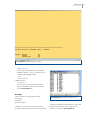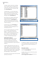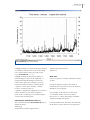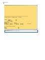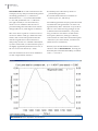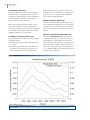
1
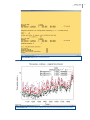
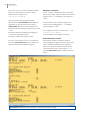
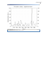
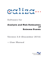
Software for Analysis and Risk Estimation of Extreme Events Version 3.0 (December 2014) — User Manual © 2011, 2014 Climate Risk Analysis ‒ Manfred Mudelsee e. K. All rights reserved. Climate Risk Analysis Caliza™ User Manual for Windows® This manual may be obtained freely from www.climate-risk-analysis.com, printed, copied, distributed or stored as a whole on your computer system. It may not be altered or parts of it extracted. This manual is furnished for distributional use only, its content may change without prior notice. Disclaimer of warranty: This manual may not be free of technical inaccuracies or typographical errors. Climate Risk Analysis ‒ Manfred Mudelsee e. K. shall not be liable to any party for any damages from any use of this manual. All information is provided “as is.” The described so�ware Caliza™ may be obtained as a demo version (limited capabilities) freely from the internet site www.climate-risk-analysis.com, stored and used on your computer system. Caliza™ may be obtained as a lite version (more, but still limited capabilities) via participating in a training course given by Climate Risk Analysis ‒ Manfred Mudelsee e. K. Caliza™ may be purchased as a fully licensed version (full capabilities) from Climate Risk Analysis ‒ Manfred Mudelsee e. K. The full license holder is allowed to use the Caliza™ executable on any computer on its premises at the address of the license holder, but not on computers on other premises. For the demo, the lite and the fully licensed version: It is not allowed to transfer the so�ware to other computers.; it is not allowed to change or sell the so�ware; it is not allowed to try to obtain the source code from the Caliza™ executable. Disclaimer of warranty: Caliza™ may not be free of technical errors. Climate Risk Analysis ‒ Manfred Mudelsee e. K. shall not be liable to any party for any damages from any use of the Caliza™ software. Caliza™ is provided “as is.” Caliza is a trademark of Climate Risk Analysis ‒ Manfred Mudelsee e. K. in Germany. The Caliza™ manual, the Caliza™ software, the Caliza™ signet and the Climate Risk Analysis ‒ Manfred Mudelsee e. K. signet are protected by copyright. Gnuplot is copyrighted 1986‒1993, 1998, 2004 by Thomas Williams and Colin Kelley. “Permission to use, copy, and distribute this software [Gnuplot] and its documentation for any purpose with or without fee is hereby granted, provided that the above [Gnuplot] copyright notice appear in all copies and that both that copyright notice and this permission notice appear in supporting documentation. Permission to modify the [Gnuplot] software is granted, but not the right to distribute the complete modified source code. Modifications are to be distributed as patches to the released version. Permission to distribute [Gnuplot] binaries produced by compiling modified sources is granted, provided you (1) distribute the corresponding source modifications from the released version in the form of a patch file along with the binaries, (2) add special version identification to distinguish your version in addition to the base release version number, (3) provide your name and address as the primary contact for the support of your modified version, and (4) retain our contact information in regard to use of the base software. Permission to distribute the released version of the [Gnuplot] source code along with corresponding source modifications in the form of a patch file is granted with same provisions 2 through 4 for binary distributions. This software [Gnuplot] is provided ‘as is’ without express or implied warranty to the extent permitted by applicable law.” Adobe InDesign is a trademark of Adobe Systems Incorporated in the United States of America and/or other countries. Windows and Windows XP are trademarks of Microsoft Corporation in the United States of America and/or other countries. Caliza™ Version 3.0 December 2014 Climate Risk Analysis ‒ Manfred Mudelsee e. K. Kreuzstraße 27, Heckenbeck, 37581 Bad Gandersheim, Germany HRA 20 13 94 (Amtsgericht Hannover) www.climate-risk-analysis.com Caliza 3.0 User Manual What is Caliza? 1 Getting Started 2 Part 1: Time Interval Extraction 7 Part 2: Extreme Events Detection 8 Part 3: Magnitude Classification 14 Part 4: Risk Estimation 17 Part 5: Bootstrap Simulations 21 Exiting Caliza 23 References 24 Internet Links 25 iii iv Caliza 3.0 User Manual Caliza 3.0 User Manual What is Caliza? Caliza is a computational tool to perform nonstationary risk analysis. Climate risk is the probability of an extremely large or small value of a climate/weather variable, such as rainfall amount or temperature. The extremes, such as floods, droughts or heatwaves, can be costly events. Full licenses of Caliza can be purchased from CRA. The CRA website has a demo version that employs an example from the book (M�������, 2014). That example (hurricanes throughout the past millennium) serves in this manual to illustrate Caliza’s functions. Nonstationarity refers to the fact that with climate changes also risk changes may be associated. Lite versions of Caliza may be obtained via participating in a training course given by Climate Risk Analysis. This version serves to fully participe in the course. It also allows to analyse any sample of size not larger than 100. Evidently, risk changes may occur in other sectors, for example, the financial system. Caliza serves also those sectors by allowing to quantify the risk, to put numbers behind a potential danger. CRA can custom-tailor Caliza to reflect your specific requirements for sensitivity analysis. Consider, for example, how sensitive flood risk estimates are to the existence or nonexistence of reservoirs on a river. Caliza allows you to analyse a time series by ● extracting time intervals of interest ● robustly detecting extreme events ● separating events into magnitude classes for detailed analyses ● testing for nonstationarity and estimating the time-dependent risk and ● performing bootstrap simulations for confidence band construction Contact CRA for your personal Caliza version, pricing, or any other information. These five parts are described in detail in this User Manual to guide your risk analysis with Caliza. Some background: Manfred Mudelsee is the founder of Climate Risk Analysis, or short: CRA. He introduced the bootstrap method to flood risk analysis in his 2003 Nature paper (M������� �� ��., 2003), working with Caliza’s predecessor, xtrend. The role of Caliza and its predecessor in the study of climate risk, has been frequently noted in professional journals which have a high impact on the climate change industry. A full treatment of the encountered statistical science is provided at book-length by M������� (2014). References are given at the end of this manual. Technical issues ● All Windows platforms (32 bit, 64 bit) ● Fortran 95 code (double-precision equivalent) ● Data size: virtually unlimited ● Interactive working environment (graphics, calculations) 1 2 Caliza 3.0 User Manual Getting Started Notation We use the symbol to denote a stroke of the “Enter” key. Required files caliza.exe caliza-demo.exe caliza-lite.exe caliza.cfg 1-8.txt cmd.exe cmd2.lnk gnuplot.exe Source CRA (licensed) CRA (demo) CRA (lite) CRA (licensed, demo, lite) CRA (licensed, demo, lite) Windows CRA (licensed, demo, lite); CRA (licensed, demo, lite) Installation (Caliza) (1) Make a Caliza folder of your choice, let us say C:\Caliza. (2) Copy the Caliza files (caliza.exe, caliza.cfg) into that folder. (3) Copy the example data file 1-8.txt into the Caliza folder. In case you have the Caliza demo version, the so�ware requires this data file; in case you have the lite or the licensed version, you do not need the file but may want to use it for exercising. Installation (cmd.exe) This is the command-line or console software. It is a part of the Windows system package, residing typically at C:\Windows\system32\ You may also download cmd.exe at the Microsoft internet site, www.microsoft.com. Installation (Gnuplot) (1) Copy the Gnuplot file (gnuplot.exe) into the Caliza folder. Adaption (cmd.exe) This step is optional but recommended to achieve a convenient work flow. (1) Make a shortcut on the desktop: > right-click on an open area on the desktop > New > Shortcut > (browse to locate cmd.exe) > Next > Finish (2) Adapt the fonts: > right-click on the shortcut symbol for cmd.exe > Properties > Font > (make your choice; for example, on my 1280 x 1024 screen, I am using for Caliza the font “Lucida Console bold 20 pt”) (3) Adapt the console window layout: > right-click on the shortcut symbol for cmd.exe > Properties > Layout > Window Size (width x height) 96 x 35 and Windows Buffer Size 96 x 6000 (4) Adapt the colours: > right-click on the shortcut symbol for cmd.exe > Properties > Colours > (make your choice; for example, I am using for Caliza a black screen text and a white/slightly yellow background) The shortcut to cmd.exe provided by CRA (cmd2.lnk), to be copied to your Caliza folder and then double-clicked, includes an adaption. Configuration file (caliza.cfg) This file prescribes the se�ing for the following parameters to be used by Caliza: ● krel ● rule ● hrelmax ● nhsrch ● ngrid ● alpha Those parameters are described in this manual. They are preset before program start and cannot be changed while the program runs (exception: parameter rule). Run Caliza It is possible to run Caliza by double-clicking (e.g., in Windows Explorer) on “caliza.exe”, but it is more convenient to use the commandline window together with the keyboard from the beginning. (1) Double-click the cmd.exe shortcut on your computer desktop: the command-line window (“Caliza window”) opens. (2) Change into the Caliza directory by typing on the keyboard: > cd C:\Caliza (followed by pressing the Caliza 3.0 User Manual Screenshot 1 Caliza welcome screen. “Enter” key: ) In case the Caliza directory is on another harddrive than C:, say F:, you may have to switch to the harddrive first: > F: > cd F:\Caliza (3) Run Caliza: > caliza.exe You see first a screen with license information and then ( ) the Caliza welcome screen (Screenshot 1). Datatype Caliza can process three types of data: ● ordinary ● extreme ● extreme times “Ordinary” means a time series (time and measured value) where the value of the climate Screenshot 2 Datatype “ordinary” file. variable is affected by both extreme events and background influence. The example series 1-8.txt is of that type (Screenshot 2). 3 4 Caliza 3.0 User Manual “Extreme” means a time series consisting only of extremes. Take as example a hurricane series, where the time is the date of an event and the value is maximum wind speed (Screenshot 3). “Extreme times” is a series with just the date of an extreme known (e.g., hurricane date). Even that scarce amount of information can yield meaningful results with the help of Caliza (Screenshot 4). Data format is text (ASCII), with decimal point and time/measured values separated by spaces (e.g., Screenshot 2) or commas. The time values increase in size, they may be unevenly spaced. No missing values are allowed. Screenshot 3 Datatype “extreme” file. On the welcome screen (Screenshot 1), select your dataype (e.g., “o” ). In the Caliza demo version, the datatype (“o”) is automatically selected. Next, give path and file name of your data (e.g., “C:\data\storms\hurricanes\ hu2.dat” ). If the file is in the Caliza directory, then you need give just its name (e.g., “1-8.txt” for the example data file). In the demo version, the file name (“1-8.txt”) is automatically selected. Observation interval This option is for datatypes “extreme” and “extreme times” only. For both selections, we need this extra information about the observation interval, from which the extreme data have previously been obtained. Consider a hurricane time series of type “extreme”, where the last recorded event is from August 2005 (i.e., hurricane Katrina). It is obvious that the risk analysis depends on whether the observation interval ends in, say, December 2005 (i.e., three months without extremes) or December 2006 (i.e., fi�een months.) Note that the observation interval must bracket the time series interval. Screenshot 4 Datatype “extreme times” file. For datatype “ordinary”, the observation interval is set automatically as the interval covered by the time series (as in the Caliza demo version). Plot (time series) A second screen appears, which shows the time series (Screenshot 5). It makes sense to learn here about the options offered by Gnuplot: (1) Hovering with the mouse over the plot allows to display the co-ordinates. Caliza 3.0 User Manual Screenshot 5 Plot of time series. (2) Right-clicking on a point, and again clicking on another point allows to zoom in. Zooming out is more tedious: return ( ) and re-plot (e.g., Screenshot 6: “o” ). (3) Right-clicking on the title bar allows to print the figure, copy it to the clipboard, or change manually the background colours, fonts or line styles. (For example, you may wish to have heavier lines for the border by > Options > Line styles > Border > Width (Color) = 2 and save this via > Options > Update file wgnuplot.ini, so that in future sessions you need not re-adapt it.) (4) A stroke ( ) brings you from the Gnuplot screen to the command line. Information field (before Part 1) The command window (Screenshot 6) shows: ● data file name ● datatype ● time interval of the original series ● observation time interval ● data size Data size Caliza can process virtually unlimited volumes of data. Owing to dynamic memory allocation in Fortran 95, the only limit is set by the memory (RAM) of your computer. For example, in the analysis of data from a coral taken off the coast of east Africa (F�������� ��., 2007), the sample contained 132554 measured data points. Caliza determines the data sizes automatically. In the demo version, the data size equals 877. 5 6 Caliza 3.0 User Manual Screenshot 6 Information field (before Part 1). Caliza 3.0 User Manual Part 1: Time Interval Extraction Extraction of a time interval allows to study data aspects in greater visual detail. Typing “n” (as usual followed by ) and supplying the interval (separated by comma or by space, see Screenshot 7, and followed by ) brings the time series plot for the extracted time interval. The example (Screenshot 8) looks into [1200; 1500]. One major event at around �� 1375 shows up. Doing brings up the information field (Screenshot 6), on which you can select the original interval (“o” ) and then (a�er ) continue (“c” ). Screenshot 7 Time interval extraction. Screenshot 8 Plot of time series (extracted interval). 7 8 Caliza 3.0 User Manual Part 2: Extreme Events Detection This part is accessible only to datatype “ordinary”. Here, the extreme events have to be detected against a background trend. Caliza estimates time-dependent background and variability robustly by means of runningmedian and running-MAD smoothing, respectively. This has the advantage that the extreme values do not bias the estimation result. (MAD is the median of absolute distances to the median.) The strength of the smoothing is described by a parameter. As an extreme event is considered what is above background plus a factor (threshold factor) times the variability. Formulas are given in the Climate Time Series Analysis book (M�������, 2014: Section 4.3.3 therein). Smoothing parameter, k The smoothing-strength parameter k determines the width of the running window (2k + 1 points), in which the median and MAD are calculated. The statistical technique of cross-validation can help adjusting parameter k. Caliza offers the support of two cross-validation functions: L1-norm and median criterion (M�������, 2014: Equations 4.58 and 4.59 therein). Caliza first gives the relative minima of both functions (Screenshot 9) and then (a�er ) plots them (Screenshot 10). The minima indicate a smoothing selection, for which relevant features in the data may be seen. Screenshot 9 Information field (before cross-validation for background estimation). Caliza 3.0 User Manual It is essential not to ignore the knowledge about the climatology or physics of the process that generated the data. Consider the example time series 1-8.txt, which has a time resolution of 1 year and contains indicators of hurricane events over the past millennium (Screenshot 5). Here we set k = 8, which means a window width of 17 years, because we consider, or have prior knowledge, that background and variability changes happen on that timescale. The cross-validation functions are calculated for a range of k values, 3 ≤ k ≤ n × krel, where n is the data size and krel is set in the configuration file. Since cross-validation calculations are computing-intensive, it may be an option to give krel a relatively small value (say, 0.05) if n is very large. Technically, do to leave the cross-validation plot (Screenshot 10), and a screen similar to Screenshot 9 appears, where you are asked for your k selection (“8” ). Screenshot 10 Cross-validation functions for background estimation. C_1(k) and C_m(k) is the L1-norm and median-criterion cross-validation function, respectively. 9 10 Caliza 3.0 User Manual Next, the time series (datatype “ordinary”) is plo�ed together with estimated timedependent background and two threshold selections (Screenshot 11). Caliza supports threshold-factor selection also graphically: zooming, logarithmic transformation (if all data values are above zero), testing three threshold factors simultaneously, etc. Threshold factor, z The choices z = 2.0 and z = 4.0 (Screenshot 11) show: (1) Smaller (larger) z values lead to more (fewer) extreme events and therefore to smaller (larger) statistical errors in the subsequent risk estimation. (2) Smaller (larger) z values may, however, also let more (fewer) non-extreme events (from the background) appear as extreme events and bias the estimation. Decision tree (Part 2) You can at this stage (a�er , Screenshot 12) choose from the following options how to continue: ● change plot se�ing (“p” ) ● set/test threshold factor z (“t” ) ● change smoothing parameter k (“b” ) ● return to Part 1 (“1” ) It is therefore wise to “play”: try a first threshold value z, perform risk estimation (Parts 4 and 5), then return to Part 2 and select another z, until the results appear suitable. Here for 1-8.txt, let us test thresholds z = 2.0, 5.2 and 8.5, make a logarithmic transformation, zoom vertically and increase the font size: > “t” > “t” > “2.0, 5.2, 8.5” , then ( ) > “p” > “g” , then ( ) > “p” > “v” > “0.4, 18.0” and (via gnuplot title bar) > Options > Choose font > Size 20. This brings us to Screenshot 13. Screenshot 11 Time series data, background and two threshold selections. Caliza 3.0 User Manual Screenshot 12 Extreme events detection. Screenshot 13 Time series data, background and three threshold selections (log, zoom). 11 12 Caliza 3.0 User Manual Here for 1-8.txt, let us follow M������� (2014: Figure 4.17 therein) and set (a�er ) the threshold factor equal to 5.2: > “t” > “s” > “5.2” A�er the plot of data, background and threshold (as in Screenshots 11 or 13) have appeared ( ), the decision tree for Part 2 (Screenshot 14) shows the information on: ● data (file name, datatype, time intervals, data size) ● extremes detection se�ing (smoothing parameter k, threshold factor z) ● number of detected extreme events In case of our analysis of 1-8.txt, a number of 47 events (Screenshot 15) results, which are analysed further in the following parts. Negative extremes So far, we have considered positive extremes, above a threshold, which are detected as above background + z × variability, with a positive z value. Caliza permits also to analyse negative extremes, below background + z × variability, with a negative z value. For example, the data of 1-8.txt with z = ‒3.0, > “t” > “s” > “‒3.0” , yield a number of 10 negative extremes. Scaled extreme values The extreme values are further scaled by subtracting the background value from a data value and then dividing by the variability (M�������, 2014: Section 6.1.4 therein). The scaled extremes series is then (a�er “c” ) plo�ed (Screenshot 15). Continue with to Part 3. Screenshot 14 Extreme events detection, after threshold factor setting. Caliza 3.0 User Manual Screenshot 15 Scaled extreme value time series. 13 14 Caliza 3.0 User Manual Part 3: Magnitude Classification This part (Screenshot 16) is accessible (with “m” ) to datatypes “ordinary” and “extreme” only. Here, the detected and scaled extremes can be classified according to their magnitude. Number of magnitude classes, l Caliza allows up to l = 3 magnitude classes. The standard choice is simply l = 1. It may in cases be meaningful to study more classes. For example, M������� �� ��. (2003) analysed flood risk in European rivers and distinguished between minor and heavy floods (i.e., l = 2). The empirical distribution function of the scaled extreme values (Screenshot 17) helps to select the number of classes and their bounds ( returns). Input l and do . Screenshot 16 Magnitude classification. Class-bound selection (for l ≥ 2) can be done in two ways. First, you can divide the range of scaled extreme values evenly (“e” ). Second, select bound(s) per hand (“h” ). If you have l = 2 magnitude classes, then give the one class bound that separates both classes (e.g., Screenshot 18: “7.0” ). If you have l = 3 magnitude classes, then give the two class bounds (separated by comma or space) that separate the three classes. In case of our analysis of 1-8.txt, we select l = 1 (“1” ). The extreme event dates are shown as bar chart (Screenshot 19). Return ( ). The information field (Screenshot 20) shows the selected magnitude classes. Continue with “c” to Part 4. Caliza 3.0 User Manual Screenshot 17 Empirical distribution function of the scaled extreme values. Screenshot 18 Magnitude classification, selection of class bound(s). 15 16 Caliza 3.0 User Manual Screenshot 19 Bar chart plot of dates of extreme events. Screenshot 20 Magnitude classification, selected classes. Caliza 3.0 User Manual Part 4: Risk Estimation This part (Screenshot 21) is accessible to all datatypes. If we have “ordinary” data, we first detect the extremes (Part 2) and then classify them according to their magnitude (Part 3); if we have “extreme” data, we first put them into magnitude classes (Part 3). If we have “extreme times” data, that is, just the dates the extreme events occurred, we do not need to visit Parts 2 or 3. Cox�Lewis test for constant risk This is a simple yet powerful test (M�������, 2014: Section 6.3.2 therein) of the null hypothesis “time-constant risk of an extreme event per time unit.” The result (a�er “t” , Screenshot 22), consisting of the test statistic, u, and the P-value, is the basis for analysing possibly time-dependent risk curves. Screenshot 21 Risk estimation. Cross-validation Cross-validation is a first step for risk estimation that assists in bandwidth selection (M�������, 2014: Section 6.3.2 therein). The minimum of the cross-validation function (a�er “k” , Screenshot 23), C(h), given on the screen in the subsequent window (a�er , Screenshot 24), may indicate a smoothing bandwidth, h, suitable for seeing the ups and downs of the risk curves for your data. Remember that cross-validation is just a guideline. Background knowledge about the data may also be used. Technical detail: C(h) is calculated for h up to hrelmax × span of time series, in nhsrch steps. Both parameters are set in the configuration file. 17 18 Caliza 3.0 User Manual Screenshot 22 Cox–Lewis test for constant risk. Screenshot 23 Risk estimation, cross-validation function. The minimum is at h = 185 a. Caliza 3.0 User Manual Screenshot 24 Bandwidth selection. Type in the bandwidth to be selected for risk estimation. For the example data (1-8.txt), we select h = 50 a (Screenshot 24: “50” ).Risk estimation The risk per time unit (also called occurrence rate) is determined with kernel estimation (M�������, 2014: Section 6.3.2 therein). The kernel bandwidth, h, has to be set for all magnitude classes. 19 20 Caliza 3.0 User Manual Screenshot 25 shows risk estimation for the example (1-8.txt), analysed with a backgroundsmoothing parameter k = 8, a detectionthreshold factor z = 5.2, a kernel bandwidth h = 50 a and pseudodata rule = ”reflection” (see right column). h was selected not by means of cross-validation but on basis of prior knowledge about decadal-scale climate changes (M�������, 2014: Figure 6.9 therein). The curve shows a peak in occurrence rate at around �� 1200 to 1300, up- and downwards trends, and so forth. The question after the statistical significance of those features is analysed by means of a confidence band (Part 5). The overall trend, over the full time span, is not highly significantly different from zero, as the Cox‒Lewis test informs (P = 0.08). Our risk estimation involves more mathematics and computational statistics: Screenshot 25 Time-dependent risk estimation. ● boundary bias reduction by means of pseudodata generation ● Gaussian kernel function evaluation in Fourier space (i.e., efficiency) Pseudodata generation may be performed with two different rules (parameter rule in the configuration file). Rule “reflection” may be advisable for cases without strong changes in risk at the time-interval boundaries, “two-point” may provide for such data a second estimation option. (However, datatype “ordinary” with extremes at either interval bound requires “reflection”.) For more details, see M������� (2014: Section 6.3.2 therein). Return ( ) to the information field, which is similar to that in Screenshot 21, showing additionally the selected bandwidth(s). Continue with “c” to Part 5. Caliza 3.0 User Manual Part 5: Bootstrap Simulations This part (Screenshot 26) is the final step in climate risk analysis with Caliza. We determine a confidence band for the estimated timedependent occurrence rate. This is accessible to all datatypes, subsequent to a risk estimation (Part 4) performed for all magnitude classes. Information field (before Part 5) This field provides you with information about the sample: file name, datatype, time intervals, data size, magnitude classification, number of extremes per class and selected bandwidth per class (Screenshot 26). From here you can either go back to previous parts (Parts 4 and, possibly, 3, 2 or 1) or enter the bootstrap simulations (“b” ). Screenshot 26 Bootstrap simulations. Bootstrap simulations Caliza generates an artificial extreme events series (with same statistical properties as the original) and repeats the risk curve estimation. The number of such bootstrap simulations is between 200 and 10000, a typical value is 2000 (M�������, 2014). From the 2000 copies of the simulated risk curves, Caliza calculates a confidence band (M�������, 2014: Algorithm 6.1 therein). Statistical details: The band is of percentile-t type (Screenshot 27): Its constructions requires, again, considerable amounts of mathematics and computational statistics: ● Studentization ● whole-array operations (efficiency) 21 22 Caliza 3.0 User Manual Computing efficiency Bootstrap simulations (and cross-validation calculations) are computationally expensive. An efficient implementation of the mathematics and statistics is therefore mandatory to keep computing costs reduced. This is one of the reasons (the other is accuracy) why Caliza has been programmed in Fortran 95, which has been the major language for scientific computing for the past decades (together with C/C++)―and still is. Confidence interval parameters Two parameters are used for constructing the confidence band: ● parameter alpha gives the confidence level (1 ‒ alpha) ● parameter ngrid determines the number of time points for which the occurrence rate (with confidence interval) is calculated. Both parameters alpha (a typical value is 0.1, that means, a 90% confidence level) and ngrid (a power of two, a typical value is 2048) are preset in the configuration file. Random number generator Caliza uses state-of-the-art generation of random variables and numbers. For each session, you need once seed the random number generator by supplying some arbritrary negative integer. Results: significant highs and lows The result (Screenshot 27) of the analysis of the hurricane proxy series (1-8.txt) shows: Although the overall trend may not be different from zero (Part 4), there is a significant high at around �� 1200 to 1300, with a occurrence rate of 0.09 events per year. See B������ �� ��. (2008) and M������� (2014: Section 6.3.2 therein) for more details. Screenshot 27 Time-dependent risk estimation with bootstrap confidence band (90% level). Caliza 3.0 User Manual Exiting Caliza A�er the bootstrap simulations and the results plot, you are brought back ( ) to the information field (Screenshot 26). Here you have several choices. Going back to Part 4 (“4” ), you can select another kernel bandwidth, h, and then repeat the bootstrap simulations (all datatypes). Back in Part 3 (“3” ), you can make a different magnitude classification (datatypes “ordinary” and “extreme”). Back in Part 2 (“2” ), the extremes detection (background-smoothing parameter, k, and detection-threshold factor, z) can be changed (datatype “ordinary”) and the analyses repeated. Screenshot 28 Caliza exit screen. Part 1 can be visited (“1” ) to inspect other time intervals (all datatypes). If you are satisfied with the se�ing at this stage (Screenshot 26), you can leave Caliza and output your results (“x” ). The Caliza exit screen (Screenshot 28) displays the names and contents of the three output files: ● caliza-1.dat: background, variability, threshold ● caliza-2.dat: extreme event times ● caliza-3.dat: hypothesis test, estimated risk curves Each file contains also a header with information on the configuration-file se�ing, data, extremes detection, magnitude classification, risk estimation and bootstrap simulations. 23 24 Caliza 3.0 User Manual References B������ MR, B������ RS, M������� M, A����� MB, F������ P (2008) A 1,000-year, annually-resolved record of hurricane activity from Boston, Massachuse�s. Geophysical Research Le�ers 35: L14705. [doi:10.1029/ 2008GL033950] F�������� D, D����� RB, M�C������ M, M������� M, V����� M, M�C������� T, C��� JE, E����� S (2007) East African soil erosion recorded in a 300 year old coral colony from Kenya. Geophysical Research Le�ers 34: L04401. [doi: 10.1029/2006GL028525] M������� M (2014) Climate Time Series Analysis: Classical Statistical and Bootstrap Methods. Second edition. Springer, Cham, xxxii + 454 pp. [ISBN: 978-3-319-04449-1, Vol. 51 of Atmospheric and Oceanographic Sciences Library] M������� M, B������ M, T������� G, G�������� U (2003) No upward trends in the occurrence of extreme floods in central Europe. Nature 425: 166–169. Caliza 3.0 User Manual Internet Links Book (M�������, 2014): sample PDF, links to data and further so�ware h�p://www.manfredmudelsee.com/book Caliza: manual and demo version h�p://www.climate-risk-analysis.com/so� /caliza Climate Risk Analysis company website h�p://www.climate-risk-analysis.com Microso� website h�p://www.microso�.com 25