Download Smart Motherboard

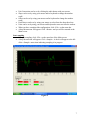
Smart
Motherboard
Data Acquisition and Display Software User Manual
Version 2.1.3
Rev 1.1
December 2003
1
Table of Contents
I.
Quick Start
II.
Screens
a. About
b. CommPort
c. Configuration
d. Main
e. Set Data Interval
f. Swap Color
III.
Appendix
a. Sample Data Files
b. Sample Linear Calibration Sheet
c. Sample Polynomial Calibration Sheet
d. Sample Peak File
2
I. Quick Start
Hardware ready
Insure that the Smart Motherboard is powered and connected to your PC as described in
the Hardware User Manual.
Launch software
• Double click the Smart Motherboard (SMB) icon on your desktop.
• The Main screen of the MicroStrain Data Acquisition and Display software will
appear.
• The default configuration will be automatically loaded and the screen will appear
like the example shown in figure 1.
Figure 1.
3
Set serial port
• On the menu bar of the Main screen, click <Tools>.
• A drop-down menu will appear. Click <Comm Port>.
• The Comm Port screen will appear as shown in figure 2.
Figure 2.
•
•
•
•
•
Using your mouse and/or keyboard, enter the number of the serial port that you
have used to connect your PC to the Smart Motherboard into the Select Comm
Port number scroll.
N.B. This number scroll accepts values between 1 and 16.
Click <Detect>. The software will attempt to poll the Smart Motherboard, and if
successful, will return a message indicating ‘Smart Motherboard found on serial
port X’. Click <OK> to close the message.
If the detect is unsuccessful, a message will be returned indicating ‘Smart
Motherboard not found on serial port X’. Click <OK> to close the message and
proceed with troubleshooting the communication failure before proceeding further
with Quick Start.
To return to the Main screen, click <OK>.
4
Set configuration
• On the menu bar of the Main screen, click <Tools>.
• A drop-down menu will appear. Click <Configuration>.
• The Configuration screen will appear.
• As stated above, the default configuration will be automatically loaded and the
screen will appear like the example shown in figure 3.
Figure 3.
5
•
Click the tab entitled ‘Channels 4-7’ and that tabs’ contents will become visible as
shown in figure 4.
Figure 4.
•
•
•
Smart Motherboards come with from 1 to 8 channels populated. The channel
names are designated 0 through 7. Determine which channels are populated on
your particular hardware configuration.
On each of the tabs (Channels 0-3 and Channels 4-7), click the appropriate
checkbox (a check appears) to indicate which channels are populated in your
configuration. Insure that unpopulated channels have no checks in their
checkboxes. These checkboxes are found on the top line of each tab; the line is
entitled ‘Channel’.
For purposes of this Quick Start, insure that the default channel parameters are set
for each active channel, i.e., those channels that you have checked. The values
are as follows:
o Unit Conversion = Linear
o Slope = 1
o Offset = 0
o Peak Detect = None
o Units = Volts
6
•
•
•
•
•
•
•
Unit Conversion can be set by clicking the radio button with your mouse.
Slope can be set by using your mouse and/or keyboard to change the number
scroll.
Offset can be set by using your mouse and/or keyboard to change the number
scroll.
Peak Detect can be set by using your mouse to select from the drop-down box.
Units can be set by using your mouse and keyboard to enter text into the textbox.
When you have completed the configuration, click <File> on the menu bar.
A drop-down menu will appear. Click <Return> and you will be returned to the
Main screen.
Start sampling
• To begin sampling, click <File> on the menu bar of the Main screen.
• A drop-down menu will appear. Click <Sample>. A check will appear to the left
of the <Sample> menu item indicating sampling is in progress.
Figure 5.
7
•
•
•
Continuous sampling will begin and the voltage values returned from each
channel will be displayed in the Volts textbox contained in the Channel frames. In
the example (figure 5), we see channels 0 and 1 as active, with channel 0
currently reporting -0.145 volts and channel 1 currently reporting -1.731 volts.
Recalling that we set our Gain at 1 and our Offset at 0 for each of these channels
on the Configuration screen, we see Scaled Values of -0.145 volts and -1.731
volts, meaning that the scaling coefficient is operating correctly. Refer to the
configuration screen for details of the scaling coefficient operation.
We also see that our graph is visualizing the continuous sampling by showing us
the individual channels voltage values over time.
Stop sampling
• To stop sampling, click <File> on the menu bar.
• A drop-down menu will appear. Click <Sample>. The check to the left of the
<Sample> menu item will disappear and sampling will end.
Congratulations!
You’re off and running! Refer to the individual screen sections and the appendix
contained elsewhere in this manual to discover all the functions that Smart Motherboard
software provides. You are also welcome to contact our technical support staff on any
matter at [email protected].
8
IIa. About
Main screen: click <Help>, click <About>.
The About screen is for information purposes only and relates 1) the software name and
version, 2) the copyright, and 3) the company name, address, website and telephone.
To return to Main screen:
• Click <OK> to return to Main screen.
9
IIb. CommPort
Main screen: click <Tools>, click <Comm Port>.
The Comm Port screen allows the user to detect the Smart Motherboard and to set the
serial port for communication with the Smart Motherboard.
To detect the Smart Motherboard:
• Using your mouse and/or keyboard, enter the number of the serial port that you
have used to connect your PC to the Smart Motherboard into the Select Comm
Port number scroll.
• N.B. This number scroll accepts values between 1 and 16.
• Click <Detect>. The software will attempt to poll the Smart Motherboard, and if
successful, will return a message indicating ‘Smart Motherboard found on serial
port X’. Click <OK> to close the message.
• If the detect is unsuccessful, a message will be returned indicating ‘Smart
Motherboard not found on serial port X’. Click <OK> to close the message and
proceed with troubleshooting the communication failure before proceeding
further.
To set the serial port:
• Using your mouse and/or keyboard, enter the number of the serial port that you
have used to connect your PC to the Smart Motherboard into the Select Comm
Port number scroll.
• N.B. This number scroll accepts values between 1 and 16.
To return to Main screen:
• Click <Ok> to return to Main screen.
Notes:
• Each time you start the application, the application reads the MS-Windows
system registry and retrieves the previously used serial port number from the
registry. That number is automatically used by the application for communication
with the Smart Motherboard unless otherwise changed in the Comm Port screen.
There is no need to enter the Comm Port screen each time you start the
application.
• Whenever you do enter the Comm Port screen, the current serial port number
(whether retrieved from the registry or previously changed in the application) will
be entered automatically in the Select Comm Port number scroll.
• Whenever you exit the Comm Port screen, the application automatically writes
the current serial port number to the MS-Windows system registry.
• Finally, the first time you start the application after installation, you will receive a
‘0’ (zero) in the Select Comm Port number scroll, indicating that you need to
select a valid serial port.
10
IIc. Configuration
Main screen: click <Tools>, click <Configuration>.
The Configuration screen allows the user to 1) activate/de-activate channels, 2) set scale
values to either linear or polynomial scaling, 3) set peak detection, 4) open, save or save
default configurations, and 5) configure other aspects of the Smart Motherboard
environment including a) saving either volts or scale values to file, b) graphing either
continuously or by auto-scaling during sampling, c) changing the upper and lower bounds
of the graph Y-axis to suit particular scaling configurations, and d) setting the Smart
Motherboard’s internal sample averaging.
To activate/de-activate a channel:
• Smart Motherboards come with from 1 to 8 channels populated. The channel
names are designated 0 through 7. Determine which channels are populated on
your particular hardware configuration.
• On each of the tabs (Channels 0-3 and Channels 4-7), click the appropriate
checkbox (a check appears) to indicate which channels are populated in your
configuration. Insure that unpopulated channels have no checks in their
checkboxes. These checkboxes are found on the top line of each tab; the line is
entitled ‘Channel’.
• N.B. If you activate channels which are not populated, i.e., no DEMOD card
and/or sensor exists, you will receive spurious data on that particular channel and
even though displayed, it should be disregarded.
To scale data linearly:
• These procedures apply to the Channels 0-3 and Channels 4-7 tabs.
• N.B. Each sensor’s raw voltage output can be scaled (converted) to actual units of
measurement using the ‘Linear’ Unit Conversion. Please refer to the Sample
Linear Calibration Sheet section in the Appendix of this manual to calculate the
Slope and Offset values needed for each active channel. When you have
calculated those values from your actual calibration documentation, continue with
this procedure.
• Using your mouse, select the Linear radio button in the Unit Conversion line.
• Using your mouse and/or keyboard, enter the Slope for each active channel in the
Slope number scroll.
• Enter the Offset for each channel in the Offset number scroll.
• Enter the Units name in the Units textbox (5 characters maximum).
• You may now proceed with sampling. The application will automatically apply
the formula {Scaled Value = (Volts * Slope) + Offset} to produce the Scaled
Value readout for each active channel.
To scale data with polynomials:
• These procedures apply to the Channels 0-3 and Channels 4-7 tabs.
• N.B. Each sensor’s raw voltage output can be scaled (converted) to actual units of
measurement using the ‘Polynomial’ Unit Conversion. Please refer to the Sample
11
•
•
•
•
•
Polynomial Calibration Sheet section in the Appendix of this manual to retrieve
the polynomial order and the individual polynomial coefficients needed for each
active channel. When you have discerned those values from your actual
calibration documentation, continue with this procedure.
Using your mouse, select the Polynomial radio button in the Unit Conversion line.
Using your mouse and/or keyboard, enter the Polynomial Order for each active
channel in the Polynomial Order number scroll.
Enter the individual polynomial coefficients in the appropriate a0-a10 number
scroll.
N.B. Previous polynomial coefficients above the current order may be visible.
These do not have to be ‘zero-ed’; only those contained within the current order
are factored.
You may now proceed with sampling. The application will automatically apply
the polynomial multiplication formula to produce the Scaled Value readout for
each active channel.
To set peak detection:
• N.B. Peak detect allows you to capture either the maximum or the minimum
scaled value for each channel during a sampling session. The peak (whether
maximum or minimum) is reported in the Peak textbox during sampling.
• Using your mouse, click the arrow on the Peak Detect drop-down box for each
active channel and select the peak type so that it appears as the choice in the dropdown box.
To open a configuration:
• N.B. Smart Motherboard software allows you to save one or more configurations
for reuse. A configuration includes each channels’ specific parameters including
Unit Conversion, Slope, Offset, Peak, Units, Polynomial Order and Polynomial
Coefficients as well as general settings including Save Method, Graph Method,
Y-Axis Range, Samples Averaged and Swap Colors. These configurations have
an extension of ‘.cfg’ and are saved in the Logs folder of your Smart Motherboard
software installation.
• Click <File>. A drop-down menu will appear.
• Click <Open>. A “common dialog” box named Open will appear.
• A list of the available configurations (.cfg) should be visible including
‘Default.cfg’.
• Click on a configuration (so it becomes highlighted) and click <Open>.
• The common dialog box will disappear and the configuration will automatically
load, populate the configuration screen and become the current configuration.
To save a configuration:
• N.B. Smart Motherboard software allows you to save one or more configurations
for reuse. A configuration includes each channels’ specific parameters including
Unit Conversion, Slope, Offset, Peak, Units, Polynomial Order and Polynomial
Coefficients as well as general settings including Save Method, Graph Method,
Y-Axis Range, Samples Averaged and Swap Colors. These configurations have
12
•
•
•
•
•
an extension of ‘.cfg’ and are saved in the Logs folder of your Smart Motherboard
software installation.
Set your particular configuration to suit your application.
Click <File>. A drop-down menu will appear.
Click <Save>. A “common dialog” box named Save As will appear.
You may create a new name for the configuration file in the File Name textbox or
you may select an existing file to overwrite as the configuration file. Click the
Save button. The common dialog box will disappear.
Your configuration is saved for reuse.
To save default configuration:
• N.B. When the Smart Motherboard software is first launched, it looks in the Logs
folder of your Smart Motherboard software installation for a configuration file
named ‘default.cfg’. It always uses this configuration to populate the application
on launch. If you would like your custom configuration to be the default
configuration, follow these steps.
• Set your particular configuration to suit your application.
• Click <File>. A drop-down menu will appear.
• Click <Save As Default>. The existing default.cfg will be overwritten with your
current configuration.
• In subsequent launches your custom configuration will be loaded as the default.
To set save method:
• On the Other Settings tab, locate the Save Method frame.
• Using your mouse, select the radio button for either the Volts or Scale method.
• The Volts method will cause raw volts to be saved to the data file.
• The Scale method will cause scaled values to be saved to the data file.
To set graph method:
• On the Other Settings tab, locate the Graph Method frame.
• Using your mouse, select the radio button for either the Auto-Scale or Continuous
method.
• The Auto-Scale method will scroll the graph’s X-axis to the right as time passes,
dropping leading previous data points and adding current data points.
• The Continuous method will scroll the graph’s X-axis to the right without
dropping any data points.
To graph volts or scale:
• On the Other Settings tab, locate the Graph Method frame.
• Using your mouse, check or un-check the ‘Graph Scale?’ checkbox.
• If checked, scale will be graphed during sampling.
• If un-checked, volts will be graphed during sampling.
To set Y-axis range:
• On the Other Settings tab, locate the Y-Axis Range frame.
13
•
•
•
Using your mouse and/or keyboard, enter values in the Upper Bound and Lower
Bound number scrolls which reflect the upper and lower values of the graph’s YAxis.
Normally, the Upper Bound is +5 volts and the Lower Bound is -5 volts.
When you return to the Main screen, the graph will be reset to reflect these YAxis changes and sampling will be graphed with these new bounds in place.
To set samples averaged:
• On the Other Settings tab, locate the Samples Averaged frame.
• Using your mouse, select the radio button for either1, 10, 100 or 200 samples to
be averaged.
• Normally, 100 samples are appropriate.
• This setting instructs the Smart Motherboard to internally sample the sensors 1,
10, 100 or 200 times to produce an average reading for output.
14
IId. Main
The Main screen allows the user to 1) navigate to the Comm Port, Configuration, Set
Data Interval and About screens and 2) sample, graph, tare, capture peak and save data
from the Smart Motherboard.
To navigate to the Comm Port, Configuration and Set Data Interval screens:
• Click <Tools>. A drop-down menu will appear.
• Click the name of the particular screen and the screen will appear.
• Each screen’s use is described elsewhere in this manual.
To navigate to the About screen:
• Click <Help>. A drop-down menu will appear.
• Click <About> and the About screen will appear.
• The About screen’s use is described elsewhere in this manual.
To start sampling:
• Click <File>.
• Click <Sample>. A check will appear to the left of the <Sample> menu item
indicating sampling is in progress.
• All active channels, i.e., those channels which are visible in the Channels 0-3
frame and/or Channels 4-7 frame AND have their checkbox checked, will begin
sampling.
• Raw voltage values will appear in the Volts textboxes; if applied, scaled values
will appear in the Scaled Value textboxes along with the corresponding unit
nomenclature in the Units column; if applied, peak values will appear in the Peak
textboxes.
• Coincidentally, each active channel’s voltage (or scaled value if selected on the
Configuration screen) will be graphed over time.
To stop sampling:
• Click <File>.
• Click <Sample>. The check to the left of the <Sample> menu item will disappear
indicating sampling has ended.
• The application will cease polling the Smart Motherboard and the data on the
screen will clear.
To start saving data to file:
• Click <File>.
• Click <Save>.
• A “common dialog” box named Save As will appear.
• You may create a new name for the data file in the File Name textbox or you may
select an existing file as the data file. Click the <Save> button. The common
dialog will disappear.
15
•
•
•
•
•
By default, these data files are saved in the Data Files folder of your Smart
Motherboard software installation.
A check will now appear to the left of the <Save> menu item indicating that a file
is in place to receive data anytime sampling is active.
N.B. You must have a file designated prior to the start of sampling in order to
save data to file. A file can not be selected during sampling.
N.B. This application creates a so-called ‘CSV’ file. CSV means comma
separated values and this is a simple flat file with commas used to delineate the
data. Many applications including MS-Windows Excel automatically load CSV
files into their working interfaces.
N.B. You will receive an error if you attempt to save data to an open file. Close
the file first and then re-start sampling.
To stop saving data to file:
• Click <File>.
• Click <Save>. The check to the left of the menu item will disappear indicating
saving has stopped.
• You may now open the file in any other application for viewing and further
processing.
To tare a channel:
• N.B. Tare is used to ‘zero’ a particular channel’s scaled value at any given point
in a sampling session. When Tare is applied, the current scaled value is captured
and is from then on, subtracted automatically from all subsequent scaled values.
The result of the taring is the value now reported in the Scaled Value textbox.
• To apply tare, click <Tare> and the tare will occur.
• Coincidentally the caption on the Tare button will change to Untare.
To untare a channel:
• Click <Untare>. Any tare in place will be removed and the scaled value will, from
then on, report its actual value.
• Coincidentally the caption on the Untare button will change to Tare.
To capture peak data:
• N.B. Peak is used to capture either the maximum or minimum scaled value
achieved during each active channel’s sampling session. When applied, Peak On
will automatically report the maximum or minimum scaled value achieved during
a sampling session in the Peak textbox. The capture of either maximum or
minimum peak is determined by setting on the Configuration screen.
• Prior to starting a sampling session, click <Tools>. A drop-down menu will
appear.
• Click <Peak On> and a check will appear to the left of the <Peak On> menu item
indicating that peak capture will occur during sampling.
• When sampling is stopped, the check to the left of the <Peak On> menu item will
disappear indicating that peak capture has ceased.
16
•
Coincidentally, a file named ‘Peak.csv’ will be saved in the Logs folder of your
Smart Motherboard software installation. This file records each channel’s peak
during the sampling session. This file is overwritten each time sampling is
stopped and represents only the current sampling session’s peaks.
17
IIe. Set Data Interval
Main screen: click <Tools>, click <Set Data Interval>.
The Set Data Interval screen allows the user to set the interval at which data is saved to
file. The user may save from 1-10 samples per second, 1-10 samples per minute, 1-10
samples per hour or save data as fast as it is generated (no restriction). Please refer to
figure 6 for a view of this screen. N.B. The sampling rate of the Smart Motherboard is
unaffected by these settings; the application is only throttling the number of samples
written to file over time.
To set data points per second:
• Using your mouse, click the radio button to the left of the Points per Second
number scroll.
• Using your mouse and/or keyboard, enter a value between 1 and 10.
• Click <OK> and proceed with sampling.
To set data points per minute:
• Using your mouse, click the radio button to the left of the Points per Minute
number scroll.
• Using your mouse and/or keyboard, enter a value between 1 and 10.
• Click <OK> and proceed with sampling.
To set data points per hour:
• Using your mouse, click the radio button to the left of the Points per Hour number
scroll.
• Using your mouse and/or keyboard, enter a value between 1 and 10.
• Click <OK> and proceed with sampling.
To write all data points collected to file (no restriction):
• Using your mouse, click the No Restriction radio button.
• Click <OK> and proceed with sampling.
18
Figure 6.
19
IIf. Swap Color
Main screen: click <Tools>, click <Swap Color>.
The Swap Color screen allows the user to change the colors of the graph plot lines to
match the channel color scheme of their particular Smart Motherboard configuration.
Please refer to figure 7 for a view of this screen.
Notes:
• Each Smart Motherboard comes with 1 or more channels populated. You will
notice a colored grommet on each channel’s sensor input connector (on the front
panel of the Smart Motherboard). As explained in the Hardware User Manual,
each DEMOD card is calibrated to its own sensor. The color-coding insures that
the user marries the proper sensor to the proper sensor cable through to the proper
DEMOD card. Because the color-coding varies from installation to installation,
the Swap Color function allows the user to change the plot colors in the
application to mirror the color-coding used for his particular sensors. This will
alleviate confusion as to which channel is reporting what sensor.
• Occasionally the choice of plot colors will be the same as the default graph
background color (black). In this case the user can change the graph color so that
no channels’ plot color gets lost in the background.
To set a channel plot line color:
• Using your mouse, click the radio button of the channel plot that you want to
change.
• Click <Swap>. A Color Dialog box will appear.
• Using your mouse, click the new color to be applied to the plot line.
• Click <OK>. The Color Dialog box will disappear.
• The new color will automatically be applied to the plot.
To set the graph background color:
• Using your mouse, click the radio button named ‘Graph Background’.
• Click <Swap>. A Color Dialog box will appear.
• Using your mouse, click the new color to be applied to the graph background.
• Click <OK>. The Color Dialog box will disappear.
• The new color will automatically be applied to the graph background.
To restore default plot line and graph background colors:
• Click <Default All>.
• All plot lines and the graph background will be returned to their default color
scheme.
To return to Main screen:
• Click <OK> to return to Main screen.
20
Figure 7.
21
III. Appendix
•
•
•
•
Sample Data Files
Sample Linear Calibration Sheet
Sample Polynomial Calibration Sheet
Sample Peak File
22
Sample Data Files
Format of CSV file with Volts being saved
MicroStrain Smart Motherboard
Data Acquisition and Display Software File Version 2.1.3
Date file created: 11/14/2003
Time file created: 12:30:20 PM
System Time
11/14/2003 12:30
11/14/2003 12:30
11/14/2003 12:30
11/14/2003 12:30
11/14/2003 12:30
11/14/2003 12:30
Time(Seconds)
0.05
0.46
0.86
1.27
1.68
2.09
CH0
-0.224
-0.225
-0.225
-0.225
-0.224
-0.225
CH1
0.153
0.153
0.153
0.153
0.153
0.153
CH0
-2.24
-2.25
-2.25
-2.25
-2.24
-2.25
CH1
1.53
1.53
1.53
1.53
1.53
1.53
Format of CSV file with Scaled Values being saved
(Volts of CSV above are scaled with Slope =10 and Offset = 0)
MicroStrain Smart Motherboard
Data Acquisition and Display Software File Version 2.1.3
Date file created: 11/14/2003
Time file created: 12:30:20 PM
System Time
11/14/2003 12:30
11/14/2003 12:30
11/14/2003 12:30
11/14/2003 12:30
11/14/2003 12:30
11/14/2003 12:30
Time(Seconds)
0.05
0.46
0.86
1.27
1.68
2.09
23
Sample Linear Calibration Sheet
Calculate Slope and Offset for entry into the Smart Motherboard Configuration screen
• As explained in the Hardware User Manual, each populated channel in the Smart
Motherboard is comprised of a DEMOD card and a sensor. These two
components are calibrated at the factory as a unit (hence the color coding) and a
calibration document is shipped representing their specific interoperability.
• N.B. The color coding scheme must be maintained in order to properly configure
the system.
• Please note the Slope and Offset value legend given on each calibration
document; this legend is generally found in the middle of the right hand edge of
the document.
• N.B. The Slope and Offset values given on the document may not be input
directly into the Smart Motherboard software; they must be run through the
following calculations to ready them for entry.
• The formula for Slope is: 1/Volts per Unit = Units per Volt.
• Using the sample above: 1/0.541 Volts per MM = 1.848 MM per Volt.
• Enter ‘1.848’ in the Slope number scroll; enter ’MM’ in the Units textbox.
• The formula for Offset is: Volts * 1/Volts per Unit.
• Using the sample above: -0.050 Volts * 1/0.541 Volts per MM = -0.092 MM.
• Enter ‘-0.092’ in the Offset number scroll.
• Repeat this exercise for each populated channel in your Smart Motherboard.
24
Sample Polynomial Calibration Sheet
NC-DVRT #1314-0001
6
5
4
3
2
y = 0.00135609x - 0.01218297x + 0.03265647x - 0.02439274x + 0.04763765x - 0.37357972x + 0.85449746
3
2.5
Displacement (mm)
2
1.5
Series1
Poly. (Series1)
1
0.5
0
-3
-2
-1
0
1
2
3
4
5
-0.5
Output (Volts)
Retrieve Polynomial Order and Coefficients for entry into the Smart Motherboard
Configuration screen
• As explained in the Hardware User Manual, each populated channel in the Smart
Motherboard is comprised of a DEMOD card and a sensor. These two
components are calibrated at the factory as a unit (hence the color coding) and a
calibration document is shipped representing their specific interoperability.
• N.B. The color coding scheme must be maintained in order to properly configure
the system.
• Please note the Polynomial Order and Coefficients value legend given on each
calibration document; this legend is generally found in the title at the top of the
document.
• Using the sample above, we find the following value legend: y = 0.00135609x6 0.01218297x5 + 0.03265647x4 - 0.02439274x3 + 0.04763765x2 - 0.37357972x +
0.85449746
• From this we extract:
o a Polynomial Order of 6 which we input into the Polynomial Order
number scroll,
o Polynomial Coefficient 0.85449746 which we input into the a0 number
scroll,
o Coefficient - 0.37357972 which we input into the a1 number scroll,
o Coefficient 0.04763765 which we input into the a2 number scroll,
o Coefficient - 0.02439274 which we input into the a3 number scroll,
25
•
o Coefficient 0.03265647 which we input into the a4 number scroll,
o Coefficient -0.01218297 which we input into the a5 number scroll,
o Coefficient 0.00135609 which we input into the a6 number scroll.
Repeat this exercise for each populated channel in your Smart Motherboard.
26
Sample Peak File
MicroStrain Smart Motherboard
D A and D S File Version 2.1.3
PEAK FILE
Channel
Time
CH0
CH1
CH2
CH3
CH4
CH5
CH6
CH7
11/17/2003 11:22
11/17/2003 11:22
Scaled Value
-0.206
0.157
0
0
0
0
0
0
Peak Type
(0=None 1=Min 2=Max)
1
2
0
0
0
0
0
0
27