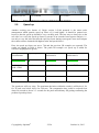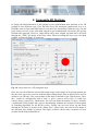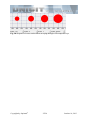
Download UNIGIT RIGOROUS GRATING SOLVER VERSION 2.01.03

UNIGIT RIGOROUS GRATING SOLVER
VERSION 2.01.03
TUTORIAL
Developed by:
Optimod
Ricarda-Huch-Weg 12
D - 07745 JENA
GERMANY
phone: +49 03641 825944
cell phone: +49 162 9067015
email: [email protected]
Copyright by Optimod
1/26
October 16, 2013
Table of Content
Table of Content ......................................................................................................................... 2
List of Tables .............................................................................................................................. 2
Introduction ................................................................................................................................ 3
1. Basic Examples .................................................................................................................. 4
1.1. Plane interface and thin film ........................................................................................ 4
1.1.1. Plane Interface ...................................................................................................... 4
1.1.2. Anti-Reflective Coating ....................................................................................... 5
1.2. Basic grating example ................................................................................................. 6
1.2.1. Preparing the computation ................................................................................... 6
1.2.2. Running a convergence test .................................................................................. 9
1.2.3. Running an AOI loop ........................................................................................... 9
1.2.4. Need to know more ? ......................................................................................... 11
2. One-dimensional gratings ................................................................................................ 13
2.1. Single Layer Gratings ................................................................................................ 13
2.2. Simple Multilayer gratings ........................................................................................ 14
2.3. Sloped gratings .......................................................................................................... 16
2.4. Complex Multilayer Stacks ....................................................................................... 18
2.5. Gradient gratings ....................................................................................................... 20
3. Two-dimensional gratings ................................................................................................ 22
3.1. Grating types.............................................................................................................. 22
3.2. Speed up .................................................................................................................... 23
4. Composite 2D Gratings .................................................................................................... 24
5. Acronyms ......................................................................................................................... 26
List of Tables
Table 1:
Zero order transmission of a dielectric grating ....................................................... 9
Table 2: Diffraction efficiencies (0. order transmission) for different 1D gratings ............. 18
Table 3: Zero order efficiencies in TE- and TM-polarisation in reflection (RE, RM) and
transmission for the parallel multilayer grating ....................................................................... 20
Table 4: Zero order efficiencies in TE- and TM-polarisation in reflection (RE, RM) and
transmission for the non-parallel multilayer grating ................................................................ 20
Table 5:
Reflection efficiencies (0. Order) for 3 different 2D grating realizations ............ 23
Table 6:
Reflection efficiencies (0. Order) for the example in table 3 with 2D speed up .. 23
Copyright by Optimod
2/26
October 16, 2013
Introduction
Unigit Version 2.01.01 provides some example stacks which come with the regular
installation. After installation, there are the following stack files available in the subfolder
“Stacks”:

interface_1d.ust:
plain interface between air (n = 1) and dielectric (n = 1.5),

arc_1d.ust:
a plain interface with an anti-reflective coating,

dielgrat_1d.ust:
a dielectric grating (n = 1.5),

algrat_1d.ust:
a metallic grating (Aluminum),

PR_BARC_1d.ust:
a photo-resist grating on a Silicon substrate with a bottom anti-
reflective coating (BARC),

two_layer_1d.ust:
a double layer Chromium grating on a dielectric interface,

slope_diel_1d.ust:
a symmetric triangular grating in a dielectric material,

slope_diel_1c.ust:
same as previous one but for C-method solver,

gradient_1d.ust:
a gradient index grating,

rcwa_dsin_1d.ust:
a coated sinusoidal grating with parallel interfaces,

ccm_dsin_1d.ust:
same as previous one but for C-method solver,

rcwa_double_1d.ust:
a triangular grating with an overcoat that exhibits a sinus profile,

ccm_double_1d.ust:
same as previous one but for C-method solver,

stack2d_elli.ust:
a 2D grating assembled by a patterned dielectric on Si-substrate,

stack2d_arbi.ust:
same as previous but with arbitrary instead of ellipse filling ,

stack2d_rect.ust:
same as previous but with patch filling ,

composite_2d.ust:
a 2D composite grating.
In the following, it will be briefly explained how to run these examples in order to give some
idea about the prospects of Unigit. Additional assistance can be obtained if necessary by
means of the context sensitive help by pressing F1 or clicking the “?” button.
Before plunging into the various more advanced examples, the basic functionality of how to
run an application will be shown in more detail with some basic example.
Copyright by Optimod
3/26
October 16, 2013
1. Basic Examples
1.1.
Plane interface and thin film
1.1.1. Plane Interface
After starting UNIGIT select the input file interface_1d.txt by means of the SELECT button
of the STACK group. (The name of the stack file is then shown under ACTIVE STACK
FILE.) Check the radio button Theta_i in the LOOP group to run a loop over the angle of
incidence (AOI) and insert a start and a stop value as well as a step width (0; 89; 1 – meaning
run from 0 through 89 degrees in step of one). Insert a wavelength value in the corresponding
field (don’t care much – the refraction index is fixed) and insert the truncation order from ..
to.. (0; 0). Then verify the output conditions by clicking the EDIT button in the OUTPUT
group (Select: Single Files; New File; Efficiency; Output Orders from 0 to 0, Check
Reflection). Define the location where to write the result file under SAVE RESULTS IN and
start the computation. After the computation is finished, you can view the results by clicking
the ADD button in the RESULT FILE(S) group and selecting the corresponding reflection
files with the extension *.re and *.rm for TE (s) and TM (p) polarization, correspondingly.
The result should look similar to that shown in figure 1. You can easily see the 4% reflection
for both polarizations at normal incidence and the Brewster angle at about 56 degrees. Of
course you can choose a finer angular grid to find the zero in TM at 56.31 degrees.
Copyright by Optimod
4/26
October 16, 2013
Fig. 1: Reflection vs. AOI from a plain interface (n = 1.5) for TE- and TM-polarized light
1.1.2. Anti-Reflective Coating
Select the input file arc_1d.txt and check the radio button Lambda in the LOOP group to run
a loop over the wavelength and insert a start and a stop value as well as a step width (0.4; 0.7;
0.02 – meaning run the wavelength from 400 nm through 700 nm in step of 20 nm). Insert a 0
for the AOI and insert the truncation order from .. to.. (0; 0). Then verify the output conditions
by clicking the EDIT button in the OUTPUT group (Select: Single Files; New File;
Efficiency; Output Orders from 0 to 0, Check Transmission). Define the location where to
write the result file under SAVE RESULTS IN and start the computation. After the
computation is finished, you can view the results by clicking the ADD button in the RESULT
FILE(S) group and selecting the corresponding transmission files with the extension .te and
.tm for TE (s) and TM (p) polarization, correspondingly. The result should look similar to that
shown in figure 2. Obviously, the transmission is 100 % at 500 nm. (The AR layer was
optimized for  = 500 nm and normal incidence according to n = sqrt(n1*n2) and h = /(4*n).)
Copyright by Optimod
5/26
October 16, 2013
Diffraction Efficiency
99.900
99.800
99.700
99.600
99.500
99.400
99.300
0.400
...esults\mist000.tm
0.475
...esults\mist000.te
0.550
0.625
0.700
Fig. 2: Transmission vs. wavelength through a plain, AR coated interface
1.2.
Basic grating example
The first grating example “dielgrat_1d.ust” is a binary grating made of dielectric material. It is
made from non-dispersive material with n = 1.5. It has a period of 1 micron, and equal lines/
spaces 400 nm in height. For a grating, the convergence strongly depends on the truncation
number, i.e., where the modal expansion of the electro-magnetic fields is truncated for the
sake of numerical calculation. Therefore, it is recommended to run firstly a convergence test.
In the following, the basic work flow is explained.
1.2.1. Preparing the computation
After starting Unigit, the Central Control Board (CCB) occurs. First, it is recommended to
load the stack file to work with. This is done by clicking the SELECT button in the Stack
group (upper right). In doing so, a Windows file requester occurs as it is shown in figure 3
and one has to select the file type “*.txt” or “*.ust” for searching Unigit stack files. In this
example, the dielgrat_1d.ust was selected. As indicated in figure 4, the active stack file
appears in the CCB. The solver is detected and activated automatically due to the type of the
stack file. Usually, it has only to be changed in case one wants to run a 1D conical rather than
1D classical mount. The selected solver is shown in radio button group “Computation”
(middle left of the CCB).
Copyright by Optimod
6/26
October 16, 2013
Fig. 3: Selecting the Unigit stack file
As a next step, it is recommended to choose the loop mode and to enter the so-called input
data (it is saved to the Unigit input file, usually “UNIGIT_directory\input\input.txt”) such as
wavelength, AOI, azimuth (applies for 1D conical or 2D simulations), truncation order and
polarization (applies for 1D classical). For this basic example, the following values and
settings have to be entered:




Enter 0.5 microns for the wavelength,
Enter 0 for the AOI (Theta_i),
Select the truncation loop by clicking the “Truncation” radio button,
Enter truncation orders 1, 20 and 1 for start, end and step.
Moreover, one has to choose a location where to save the results file to by means of the edit
control field and the selection button “…” at the bottom of the CCB. After having set all these
things correctly, the CCB should look like shown below.
Copyright by Optimod
7/26
October 16, 2013
Fig. 4: Unigit Central Control Board with selected stack file
Eventually, one has to specify the flavor of output by means of the output editor tab. It is
activated just by clicking the EDIT button in the “Output” group (middle right of the CCB).
Regarding the detailed functionality of the output editor it is referred to the corresponding
section of the user manual. Related to this example, the following actions have to be done:
 Choose single files in radio button group “Output files” (upper right),
 Check the “Transmission” box in the same group (below),
 Check the radio button “New” in the same group,
 Check the output formats – “Fix” and “8 digits”,
 Choose the option “Efficiency” in the “Output value” group (upper right),
 Choose the output orders 0 through 0 (lower right),
 Check the box “Efficiency in %”.
After having done this steps correctly, the output editor should look like depicted in figure 5.
Copyright by Optimod
8/26
October 16, 2013
Fig. 5: Unigit Output Control Editor
1.2.2. Running a convergence test
Then, run the computation just by clicking the start button (or Ctr-S hotkey). The results can
be retrieved by means of the NOTEPAD button in the “Result files” group (bottom right). It
should be similar to those presented in table 1 below.
Truncation
1
2
3
4
5
6
7
8
9
10
Table 1:
TE
15.798
20.421
20.257
20.015
20.031
20.018
20.024
20.022
20.025
20.024
TM
24.333
20.129
21.623
21.246
21.428
21.361
21.411
21.39
21.41
21.401
Truncation
11
12
13
14
15
16
17
18
19
20
TE
20.025
20.025
20.026
20.026
20.026
20.026
20.026
20.026
20.027
20.027
TM
21.411
21.407
21.412
21.41
21.413
21.411
21.414
21.413
21.414
21.413
Zero order transmission of a dielectric grating
Depending on the required accuracy, a truncation between 4 and 9 seems to be appropriate.
1.2.3. Running an AOI loop
Now, you are probably interested in the diffractive behavior of this grating. To this end check
the radio button Theta_i in the LOOP group and insert (0; 60; 1) and change the grating
period to 0.3 microns (use the stack editor). Due to the changed pitch, the convergence is
supposed to be better. So, a truncation order of 5 should be sufficient in what follows.
Copyright by Optimod
9/26
October 16, 2013
However, you are free to rerun it. Next, check both Transmission and Reflection for the
output file and choose output orders minimum = -1 and maximum = 0. In addition, it is
recommended to check the “Project file” box and enter a project file name in the output
editor. Then run Unigit again.
The reflection and transmission efficiencies are depicted in figures 6 and 7 below. These plots
can be simply generated by selecting the corresponding result files and hitting the diagram
button as described in the manual (see section 1).
Diffraction Efficiency
0.120
0.100
0.080
0.060
0.040
0.020
0.000
0.000
...esults\test000.re
15.000
30.000
45.000
...esults\test000.rm
...esults\testm01.re
60.000
...esults\testm01.rm
Fig. 6: Reflection efficiencies vs. AOI for the dielgrat_1d example
Diffraction Efficiency
0.800
0.600
0.400
0.200
0.000
0.000
...esults\test000.te
15.000
30.000
45.000
...esults\test000.tm
...esults\testm01.te
60.000
...esults\testm01.tm
Fig. 7: Transmission efficiencies vs. AOI for the dielgrat_1d example
Copyright by Optimod
10/26
October 16, 2013
From the results one can see that:
 the minus first order in reflection occurs at AOI > 41.8 degrees,

the minus first order in transmission appears at AOI > 9.6 degrees,

the total energy in all propagation orders (reflection and transmission) is 100 % (energy
criterion).
1.2.4. Need to know more ?
Now assume that you are also interested to have a look at the phases, you want to see the
ellipsometry parameters or you need to know the diffraction angles. In the further two cases
you could rerun Unigit with changed settings of the output editor, in the latter case you even
cannot do this. Rerunning this simple example is not a big deal and takes only seconds.
However, when it comes to complex 2D gratings, a run can easily last several hours. In order
to avoid time consuming reruns, a smarter way was introduced in Unigit in order to retrieve
results from an example which has already been run, i.e., the information has already been
generated. The only thing what you have to do before the original (first) run of the example,
or let it better call project is to specify that and where the project information shall be saved.
This is easily in the output editor by means of checking the box “Project File” (bottom) and
entering a file name (edit control next to it).
Then, the project file can be load just by selecting a project file (extension *.upr) instead of a
stack file (see also section 6 of the Unigit manual). After having selected the before generated
project file “dielgrat_1d.upr”, the way how to generate modified results is quite similar to the
regular computation mode. One has first to specify the output conditions by means of the
output editor and then run the extraction by means of the same button which is used for
starting a regular run. A successful extraction is indicated between the CANCEL and EXIT
button. The phases for the minus first and zeroth order for reflection and transmission are
shown in figures 8 and 9, respectively.
Copyright by Optimod
11/26
October 16, 2013
Fig. 8:
Notepad output of the phases for 0. and -1. order in reflection
Fig. 9:
Notepad output of the phases for 0. and -1. order in transmission
Analogously, tan(psi) and cos(delta) or the diffraction angles can be retrieved.
Copyright by Optimod
12/26
October 16, 2013
2. One-dimensional gratings
2.1.
Single Layer Gratings
One single layer binary grating (dielgrat_1D.ust) was already treated in the previous section.
Now, we shall consider a metallic grating. Select the input file al_grat_1d.txt. It is made
from Aluminum, has a period of 0.5 microns and equal lines/ spaces being 200 nm in height.
Diffraction Efficiency
78.000
70.000
62.000
54.000
46.000
38.000
1.000
...esults\mist000.rm
10.750
20.500
...esults\mist000.re
30.250
40.000
Fig. 10: Diffraction efficiencies vs. truncation order of a metallic grating (0. order reflection)
Again, you should first run a convergence test. Check the TRUNCATION button, enter
(1;40;1) to specify the truncation loop and 0.7 for the wavelength. Your convergence curves
(reflection) should look like those of figure 10. In spite of the improved models implemented
in UNIGIT, the TM-convergence (pink curve) for metallic gratings is sometimes worse
compared to TE.
The next recommendation is again a loop over the AOI (0;50,1) with a truncation setting of
25. The resulting reflection curves for the 0. and –1. order are shown in figure 11. Clearly, a
sharp change in the zeroth orders can be observed when the first orders start to propagate at
AOI = 23.57 degrees.
Copyright by Optimod
13/26
October 16, 2013
Diffraction Efficiency
80.000
60.000
40.000
20.000
0.000
0.000
...esults\mist000.re
12.500
25.000
37.500
...esults\mist000.rm
...esults\mistm01.rm
50.000
...esults\mistm01.re
Fig. 11: Reflection efficiencies (0. & 1. order) vs. AOI for a metallic grating
2.2.
Simple Multilayer gratings
There are two multi-layer stack files available which come with the installation of version
2.01.01 of Unigit:
 PR_BARC_1D.ust: A patterned photo-resist above a BARC layer on a Silicon
substrate. The grating period is 0.5 microns. The PR-lines are 300 nm high and have a
line width of 250 nm. The 100 nm thick BARC layer is not patterned.
After selecting this stack file and opening the stack editor, the window should look like shown
in figure 12.
Copyright by Optimod
14/26
October 16, 2013
Fig. 12: Unigit stack editor showing the PR_BARC_1D.ust grating stack
Obviously, the stack is assembled by two layers, a RCWA (hard transition) on top of a thin
film exactly as been described above.
 Two_layer_1D.ust:
A patterned Chromium double layer on a dielectric substrate.
The grating pitch is 0.5 microns. The geometry is depicted in figure 13. This example
gives a hint how to assemble non-binary gratings from rectangular slices. An
automated slicing tool is available in the full version of UNIGIT.
Fig. 13: Schematic cross section of the grating implemented in the file Two_layer_1D.ust.
The associated stack editor is shown in figure 14 below.
Copyright by Optimod
15/26
October 16, 2013
Fig. 14: Unigit stack editor showing the PR_BARC_1D.ust grating stack
2.3.
Sloped gratings
Unigit version 2.01.01 offers a few different ways for the simulation of sloped gratings. The
term sloped is understood as anything different from binary, e.g., sinusoidal, triangular or
trapezoid. Unigit offers two basic methods to input sloped gratings – the composite Fourier
and the composite polygon layer. The details of how this layers can be implemented are given
in the Unigit manual (see the corresponding sections in the layer editor). During the input of
this type of gratings, a slicing routine is run and a stack of RCWA-slices is generated
automatically. There is of course also another cumbersome way of building up any interface
or layer from scratch which shall be only mentioned for reason of completeness, namely
piling up RCWA slices by means of the stack editor.
However, there are alternatives for describing and simulating sloped gratings. The first
alternative are the Rayleigh-Fourier polygon and sinusoidal layer. This type of layer can be
mixed with RCWA-slices or composite layers to form a multilayer stack. When specifying
these types of layers, a special solver routine based on the Rayleigh-Fourier method will be
applied during simulation. The drawback of this method is that it is not rigorous and provides
only accurate results for shallow profiles.
Another alternative is the C-method solver. This method is based on a rigorous modal
algorithm derived from Maxwell’s equations. Not only is this algorithm usually much faster
than the RCWA, but it also provides much faster convergence and accuracy in many cases.
Copyright by Optimod
16/26
October 16, 2013
Both alternatives do not require the profile decomposition in slices resulting in the great speed
enhancement.
In the following, one example of a triangular grating shall be considered as a case study. The
grating consists of patterned dielectric material with index = 1.5. The profile is shaped as a
symmetric triangle as shown in figure 15.
Fig. 15: Unigit layer for implementing a C-method polygon “layer”
The height of the profile is 200 nm and the grating period is 1 micron. The grating is
illuminated with green light (550 nm) under oblique incidence (30 degrees). A truncation of
±20 seems to be more than sufficient for this example.
The grating has been implemented in two different ways:
 As Composite Polygon layer to be run by the RCWA solver (1D Classic)
 As C-method (CM) layer polygon to be run by the C-method solver (1C).
Two files are provided which contain these gratings – slope_diel_1d.ust and
slope_diel_1c.ust. The zeroth order transmission efficiencies are shown in the table 2 below.
File
Solver
# of Slices
Transmission TE 0
Transmission TM 0
slope_diel_1c.ust
C-method
N/A
74.97823857
87.31595748
Copyright by Optimod
17/26
October 16, 2013
slope_diel_1d.ust
RCWA
Slicing
+ 10
75.00495505
87.52453837
slope_diel_1d.ust
RCWA
Slicing
+ 25
74.98385363
87.43482951
slope_diel_1d.ust
RCWA
Slicing
+ 50
74.98059365
87.42389105
Table 2:
Diffraction efficiencies (0. order transmission) for different 1D gratings
Apparently, the results are very similar. Moreover, the RCWA results seem to converge to the
C-method results with increasing number of slices giving evidence for the correct
implementation of both methods. A similar example could also be run comparing all three
methods, i.e., the Rayleigh-Fourier approach beside the C-method and the RCWA solver.
However, here one should reduce the profile height to make sure that the RF method still
converges. It is left to the user as an exercise.
2.4.
Complex Multilayer Stacks
In section 2.2, examples for simple (binary) multilayer stacks have been already presented. In
this section, more sophisticated gratings shall be discussed assembled from several layers of
different material that are separated by arbitrary rather than straight boundaries such as for
example triangle, trapezoidal or sinusoidal interfaces. Basically, these types of gratings can be
run either with the RCWA-solver (1D classic) or, in many cases preferably, with the Cmethod solver (1D C-method). An exception are overhanging and very steep profiles
(meaning profiles with slopes close to vertical), although there are workarounds for the
former. Here, we provide two examples – a trapezoidal grating that is coated by a layer of
uniform thickness everywhere and a triangular grating over coated by a layer with an inverse
sinusoidal profile. Grating files are given for RCWA as well as for C-method simulation for
both examples.
The first example is shown schematically in figure 16. The thickness of the intermediate layer
is constant everywhere rendering the two interfaces parallel. The associated stack files coming
with the installation are rcwa_dsin_1d.ust and ccm_dsin_1d.ust.
The second example covers the more general case of non-parallel interfaces. It is shown in
figure 17. The grating is triangular and the coating exhibits a trapezoidal profile resulting in
non-parallel interfaces. In this way, so-called snowing effects occurring after the coating can
be modeled. Of course, a lateral offset can also be invoked (see Unigit v2.01.02 manual). The
associated stack files are rcwa_double_1d.ust and ccm_double_1d.ust.
Copyright by Optimod
18/26
October 16, 2013
Fig. 16:
Parallel Multilayer Grating
Fig. 17:
Nonparallel Multilayer grating
Simulations have been run for both grating types with both solvers. The results for the parallel
grating are summarized in
RCWA
RE0
RM0
TE0
CM
TM0
RE0
RM0
TE0
TM0
0.5
1.9797E-01
2.8229E-03
6.6188E-01
8.7378E-01
1.9960E-01
2.3919E-03
6.6256E-01
8.7601E-01
0.52
1.9888E-01
1.7398E-03
6.8024E-01
8.8555E-01
2.0047E-01
1.3970E-03
6.8054E-01
8.8743E-01
0.54
1.9419E-01
7.9289E-04
6.9591E-01
9.0026E-01
1.9575E-01
5.6994E-04
6.9605E-01
9.0176E-01
0.56
1.8686E-01
2.3387E-04
7.1300E-01
9.1524E-01
1.8837E-01
1.2258E-04
7.1310E-01
9.1640E-01
0.58
1.8007E-01
1.2138E-05
7.3067E-01
9.2791E-01
1.8152E-01
9.5985E-07
7.3073E-01
9.2882E-01
0.6 1.7573E-01 1.2041E-04 7.3903E-01 9.3333E-01 1.7703E-01
Table 3 and those for the non-parallel grating in Table 4. An
2.0905E-04
7.3916E-01
9.3402E-01
order truncation of ±20 and a
wavelength loop (0.5 … 0.6 µm) was selected for the two examples. Moreover, AOI’s of 60
Copyright by Optimod
19/26
October 16, 2013
degrees for the parallel and normal incidence for the non-parallel multilayer grating have been
chosen. The results are similar although there are visible differences, particularly in TMpolarization. This may mainly be debited to approximation issues in the RCWA. Comparisons
with a very accurate integral method implementation always showed very good agreement for
the C-method simulations. Furthermore, the C-method clearly outperformed the RCWA for
the given examples in terms of computation speed. Due to the large number of slices, the
RCWA was about 100 times slower compared to the C-method solver. In addition, there are
cases were the RCWA slicing becomes quite complicated when the interfaces between the
layers overlap in lateral direction. This may be the case when the distance between the
interfaces is smaller than the profile height. In spite of these clear advantages, there are many
cases were one has to rely on the RCWA. In conclusion, a careful decision whether to use
RCWA- or CM- solver is stronglrecommended.
RCWA
RE0
RM0
CM
TE0
TM0
RE0
RM0
TE0
TM0
0.5
1.9797E-01
2.8229E-03
6.6188E-01
8.7378E-01
1.9960E-01
2.3919E-03
6.6256E-01
8.7601E-01
0.52
1.9888E-01
1.7398E-03
6.8024E-01
8.8555E-01
2.0047E-01
1.3970E-03
6.8054E-01
8.8743E-01
0.54
1.9419E-01
7.9289E-04
6.9591E-01
9.0026E-01
1.9575E-01
5.6994E-04
6.9605E-01
9.0176E-01
0.56
1.8686E-01
2.3387E-04
7.1300E-01
9.1524E-01
1.8837E-01
1.2258E-04
7.1310E-01
9.1640E-01
0.58
1.8007E-01
1.2138E-05
7.3067E-01
9.2791E-01
1.8152E-01
9.5985E-07
7.3073E-01
9.2882E-01
0.6 1.7573E-01 1.2041E-04 7.3903E-01 9.3333E-01 1.7703E-01 2.0905E-04 7.3916E-01 9.3402E-01
Table 3: Zero order efficiencies in TE- and TM-polarisation in reflection (RE, RM) and transmission for the
parallel multilayer grating
RCWA
lambda
RE0
RM0
TE0
C-Method
TM0
RE0
RM0
TE0
TM0
0.5 3.6121E-02 2.3741E-02 9.1920E-01 9.5615E-01 3.7467E-02 2.5761E-02 9.2322E-01 9.5483E-01
0.52 3.8851E-02 2.4833E-02 8.8200E-01 9.5919E-01 3.9918E-02 2.6852E-02 8.8921E-01 9.5718E-01
0.54 4.6098E-02 2.5940E-02 8.4468E-01 9.6393E-01 4.6867E-02 2.7911E-02 8.5291E-01 9.6181E-01
0.56 5.5352E-02 2.5999E-02 8.0639E-01 9.6991E-01 5.5904E-02 2.7872E-02 8.1445E-01 9.6784E-01
0.58 6.4025E-02 2.5425E-02 7.7808E-01 9.7395E-01 6.4453E-02 2.7188E-02 7.8502E-01 9.7207E-01
0.6 6.9775E-02 2.4813E-02 7.6528E-01 9.7496E-01 7.0114E-02 2.6471E-02 7.7077E-01 9.7335E-01
Table 4:Zero order efficiencies in TE- and TM-polarization in reflection (RE, RM) and transmission for the nonparallel multilayer grating
2.5.
Gradient gratings
Gradient gratings are gratings that rely on a gradual change of the refraction index rather than
a stepwise index profile (as given across a common RCWA slice). One can also conceive a
gradient grating as a thin film layer with a periodically but gradually changing refraction
index. In Unigit, gradient gratings are created and described by means of the soft transition
RCWA slice (for details see Unigit manual, section layer editor). It might be of interest to
know that a gradient layer may converge to a standard RCWA slice when increasing the
number of entrances to infinity but using only a limited number of refraction index values.
A simple example will be discussed in the following. Remember the dielectric grating
“dielgrat_1d.ust” of section 1.2. Suppose that you run an AOI loop for a range of theta_i = 30
through 60 degrees. Next, setup a gradient grating with the same geometry and refraction
Copyright by Optimod
20/26
October 16, 2013
index as dielgrat_1d. This grating can be found under the name “gradient_1d.ust” in the
Unigit stack folder. It consists of 32 equidistant index values, namely 16 in a row with index
= 1.5 and 16 with index = 1. So, it resembles closely dielgrat_1d. Therefore, one would
expect a similar diffraction behavior. The zeroth order transmission versus AOI is plotted for
both cases and both polarizations in figure 18. Apparently, the results are almost the same.
The differences arise from the different internal processing of the different layer types. It is
left to the user to increase the sampling density of the gradient grating to check whether the
diffraction spectrum is converging to that of the binary grating.
Diffraction Efficiency
40.000
34.000
28.000
22.000
16.000
30.000
37.500
45.000
52.500
...radient_32_000.te
...radient_32_000.tm
...ts\dielgrat000.te
60.000
...ts\dielgrat000.tm
Fig. 18: Comparison of zeroth order transmission for a binary RCWA grating vs. a gradient
grating
Copyright by Optimod
21/26
October 16, 2013
3. Two-dimensional gratings
3.1.
Grating types
Again, there are basically three different types of 2D gratings in Unigit (see manual, layer
editor 2D), namely the patch fill, the ellipse fill and the arbitrary fill. The two latter options
are more general but in a sense less accurate. Here, a sort of equidistant discretization is done
which is quite similar to the so-called 1D gradient grating. On the other hand, the patch filling
can be considered as a sort of RCWA (hard transition) for 2D. However, it is limited to
rectangles only while the other two option enable a variety of 2D cross sections such as
ellipses, diamonds and corner rounded rectangles.
In this example of the tutorial, a simple 2D grating shall be considered which enables to
compare all three grating types directly for the same geometry. The grating consists of a 100
nm thick dielectric layer on top of a Silicon substrate. Rectangular holes with CDx = 250 nm
and CDy = 375 nm are etched into the dielectric.
This geometry has been implemented differently in three Unigit layer stacks:
 Stack2d_elli.ust
with ellipse fill option,
 Stack2d_rect.ust
with patch fill option,
 Stack2d_arbi.ust
with arbitrary (gradient) filling.
The grating was illuminated normally with a plane wave having 800 nm wavelength. The
truncation order was set to 6 meaning that 2*6+1 orders in both directions resulting in a still
quite moderate total number of 169 have been maintained during computation. This is
justified because of the low contrast material and the pitch over wavelength ratio > 1. The
Table 5 below shows the resulting zeroth order reflection for TE- and TM-polarization.
Apparently, all values are quite close to each other. The maximum deviation is about 0.2%.
This can be further reduced by increasing the sampling density of the ellipse and arbitrary
filling layers. One example is also included in the table. Here, the discretization of the ellipse
fill was increased from 512 x 512 to 2048 x 2048 (highlighted in green color). Evidently, the
results are now much closer than before.
Grating file/
Discretization
Zero Order TE Reflection/%
Zero Order TM Reflection/%
Stack2d_elli.ust
512 x 512
24.19229348
24.68655616
Stack2d_elli.ust
2048 x 2048
24.15039565
24.64946358
Stack2d_arbi.ust
24.13369369
24.63391415
Copyright by Optimod
22/26
October 16, 2013
Stack2d_rect.ust
Table 5:
3.2.
24.13640498
24.63724637
Reflection efficiencies (0. Order) for 3 different 2D grating realizations
Speed up
Another exciting new feature of Unigit version 1.02.04 upwards is the smart order
management which permits speed up factor of 10 and higher. It should be pointed out,
however, that the speed up should be very carefully used. The best way to always be on the
safe side is to verify the speed up factor by means of an extended convergence analysis, i.e.,
not only to vary the order but also the speed up factor during convergence runs and compare
the results to those obtained with highest order and speed factor 1.
Here, the speed up factor was set to 7.84 and the previous 2D example was repeated. The
results are shown in Table 6 below. The patch fill example w/o speed up is added for
reference (highlighted in green).
Grating file/
Discretization
Speed up
Zero Order TE
Reflection/%
Zero Order TM
Reflection/%
Stack2d_rect.ust
1
24.13640498
24.63724637
Stack2d_elli.ust
2048 x 2048
7.84
24.13003663
24.64187327
Stack2d_arbi.ust
7.84
24.11269207
24.62607999
Stack2d_rect.ust
7.84
24.11603230
24.62961443
Table 6:
Reflection efficiencies (0. Order) for the example in table 3 with 2D speed up
The results are still very close. The maximum deviation within the results is still below 0.1%
for TE and even below 0.05% for TM-case. The computation time could be reduced from
about 20 seconds to about 2..3 seconds for the patch and arbitrary fill grating confirming the
predicted speed up factor.
Copyright by Optimod
23/26
October 16, 2013
4. Composite 2D Gratings
In Unigit, the third dimension of 2D gratings can be implemented quite similarly as for 1D
gratings in two different ways. First, the brute force but sometimes cumbersome way is to
build the stack up from individual layers by means of the stack editor. Both the copy, cut and
paste features as well as the work with sequences (pre-manufactured sub stacks) may greatly
facilitate this approach. However, Unigit offers also a more elegant way that can be accessed
through the CONE_3D option in the layer editor. When activating this layer type, the input
window as shown in figure 19 comes up.
Fig. 19: Layer editor for a 2D-composite layer
Here, the user can define the top and the bottom cross section shape of his grating pattern just
like the same way as he is used to with the ellipse filling feature. But as opposed to it, now he
defines a real 3D body. The vertical shape of this body is defined by the vertical power. Here,
the 1 results in a straight line while a value >1 gives a convex and a value <1 results in a
concave shape, respectively. Furthermore, the user can define the number of slices. Actually,
a equidistant slicing routine takes care to automatically translate the compact 3D description
in something digestible for the RCWA solver. Finally, the user can sweep up and down
through the 3D body by means of the “Show Slice” option. Here, the cross section shape of
the activated slice number is plotted. The figure 20 below shows such a sequence of cross
sections for the body defined above.
Copyright by Optimod
24/26
October 16, 2013
Fig. 20: Sequence of cross section when sweeping through a 2D composite layer
Copyright by Optimod
25/26
October 16, 2013
5. Acronyms
AOI
AR
BARC
CCB
CD
CM
PR
RCWA
RF
TE
TM
1D
2D
3D
-
Angle of Incidence
Anti Reflective
Bottom Anti Reflective Coating
Central Control Board
Critical Dimension
Coordinate Transformation Method (a.k.a. C-method)
Photo resist
Rigorous Coupled Wave Approach
Rayleigh-Fourier (Method)
Transverse Electric
Transverse Magnetic
one-dimensional
two-dimensional
three-dimensional
Copyright by Optimod
26/26
October 16, 2013