1
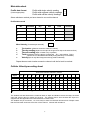
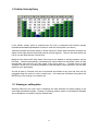
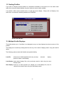
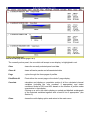
User Manual for River Form & Channel Analysis Geopacks 2005 RIVER FORM & CHANNEL ANALYSIS An application for investigating river channels By Rick Cope, Backwell School, Bristol Published by Geopacks - 2005 Contents Topic Pages Introduction ......................................................................................................................... 1 Gathering Data in the field.................................................................................................... 1 Data Formats.......................................................................................................... 2 - 3 Field recording (Profile)............................................................................................... 4 Velocity recording........................................................................................................ 5 Recording sheets ................................................................................................... 5 - 6 Initial Data Entry .................................................................................................................... 7 Main Data Entry (Spreadsheet) ............................................................................................ 8 Velocity data entry.................................................................................................. 8 - 9 Viewing or Editing data......................................................................................................... 9 Displaying Profiles .......................................................................................................... 10 Scaling Profiles.................................................................................................................... 11 Multiple Profile Displays.............................................................................................. 11 - 12 Correlating Variables ................................................................................................... 13 - 14 CardFiles .............................................................................................................................. 15 The Notebook....................................................................................................................... 16 Help ....................................................................................................................................... 16 Saving, Loading and Printing ............................................................................................ 16 System Requirements for CHANNEL • • • • • IBM compatible PC Windows 95 (or higher) 10 megabytes of free hard disk space (for program files) 4 megabytes of memory SVGA monitor (800 * 600 display recommended) GeoSoft CHANNEL This application allows the user to process field data on river channels and display or interrogates that data in a number of ways. Data is entered at the keyboard via a number of pre-formatted data-entry screens, each tailored to suit the users requirements. To enable the application to do this certain basic initial information is required (see Initial Data section) and then the user is led through a sequence of events, which record all necessary information. The notes, which follow, outline the procedures available for creation, display, storage and retrieval of this information together with advice on other facilities, which may be of use such as "help" files and the "notebook". To allow easy access the notes are divided into a number of sections; Section Topic 1 2-4 5-9 10 - 11 11 - 12 13 - 14 15 16 16 16 Gathering data in the field Data formats Data entry Displaying and scaling single profiles Multiple Profile Displays Correlating Calculated Variables Cardfile displays The Notebook facility Help Saving, Loading and Printing Information on saving, loading from disk and printing data and screen displays is also included in the relevant topic sections. These notes are also available via the on-screen help file. Simply click on Help using the menu options provided with each display. 1 Gathering data in the field Firstly a word of caution. Channel will handle draw scaled cross sections of stream and river channels up to 20 metres wide but it must be understood that working in deep or moving water can be dangerous and extreme care must be taken. The following precautions should be taken; a. b. c. d. e. f. g. Check out the location before embarking on the measuring. Look for hidden obstacles, submerged weeds or soft mud, which could pose a threat. Avoid working alone on larger or faster channels Always leave a note with someone as to where you intend to be working. Check the weather forecast. Rivers rise rapidly; don't get caught out by being on the wrong side after heavy rain has swollen a previously amiable stream. If working in fast water deeper than knee-deep face upstream. The water will not then cause your knees to buckle and you to lose your balance If in doubt, miss it out! Don't push the boat out! 1 2 Data formats There are THREE formats in which data can be recorded. Each has its merits depending on how much detail your project requires. 1. Profile and single velocity reading which gives a simple cross-section with calculated channel variables. The easiest from a data collection point of view. This, the simplest of the data formats, makes use of cross-section data and a single velocity reading to draw an accurate cross-section and calculate the relevant variables. 2. Profile and segment velocity readings in which velocity data for each unit of channel is entered. More accurate from both a calculation and display point of view with position of maximum flow being marked clearly on all cross-sections. Data format 2 3. Profile and cellular velocity readings where an MJP flowmeter is used to record velocity data at regular depths for each channel unit to give "velocity cells". These can then be used to produce both a "choropleth" display of velocities at varying depths across the profile (using up to six shading classes) and highly accurate calculations of discharge Data format At each location across the channel a number of velocity readings are taken at increasing depths. In the case of the example below each location was .5 metres apart and velocity readings taken at 10cms, 20cms, 30cms and so on. The combination of these two data sets allows a sophisticated display of the channel flow characteristics and a highly accurate calculation of discharge to be achieved. Missing data in cells bordering the channel margins which may be too shallow to measure is automatically calculated using known information from surrounding cells to extrapolate. Resulting cellular display 3 3 Field Recording Methods - Profile data There are several stages in the creation of accurate cross-sections using channel. 1 Decide on a suitable (and safe) location for your cross-section 2 Stretch a tape across the river and anchor it at each end firmly ensuring that the tape is as near horizontal as possible. To make the most of channel's section drawing try to go from the top of the bank on one side to the top of the bank on the other. Sometimes, if one bank is higher than the other it is possible to raise one end of the tape by placing it over a stone, stick or other object. 3 Decide on how far apart each channel segment will be. If you have only a small channel, say 2 metres, then to go for a distance apart of 50 cms will give you a very chunky section with little detail. To go for 25 cms or even 10 cms will take a little longer but give a far more accurate result. Obviously, you would be foolish to measure every 10 cms on a 20 metre wide channel. The increased accuracy over a more realistic segment of 50 cms is very little and a longer distance apart would be more appropriate. Channel can handle up to 200 readings on each section. 4 As you work your way across the channel a segment at a time note; a. b. c. The location (distance across the channel in metres) The dry reading (depth from the tape to the ground or tape to the water surface) The wet reading (depth of water if any is present) Repeat these at each location across the channel until the far bank is reached. 4 4 Field recording methods - Velocity recording For a standard profile with a single velocity reading...... Use the MJP Flowmeter to record the velocity of the water at around 0.6 of the channel depth. Make a note of the result in metres per second. For a profile using segment velocity readings....... Measure the velocity (in metres per second) as above but take recordings, wherever possible, for each channel segment in which water is present. In the example on the previous page you would probably end up with 3 readings, at 1.0 m's, 1.5 m's and 2.0 m's. Although water is present at 2.5 metres it is unlikely that it is deep enough to be measured. This is allowed for in any calculations and compensations are made automatically. For profiles using cellular velocity readings...... Decide upon an appropriate vertical interval for each cell reading. Don't be too ambitious! It can be quite time consuming. Assess the maximum depth you are dealing with and decide on a nice round number for your vertical interval. In the example on page 3, six cells at 10 cm intervals have been used on a channel with a maximum depth of 70+ cms. The first was made at 10 cms, the second at 20 and so on. This appears to be quite effective. Too few and the display is "chunky" and lacks detail, too many and it can be too "fussy", time consuming and confusing when displayed. 5 Entering the data on recording sheets The record sheet has two sections. The first for locational data and "set-up" information, the second for the main profile data. Initial information Location (The name of the stream or river) Site (this can be just a reference number or, as this entry is used as a variable in any correlation work, it could be more accurate information such as distance downstream or height above sea level .) Grid Reference ________________ (a four or six figure reference - optional) Number of readings ______ (the number of segments making up the profile) Distance apart _____ metres (horizontal interval of segments) Vertical interval of cell velocity readings _____ cms (as it says, optional) 5 Main data sheet Profile with single velocity reading Profile with segment velocity readings Profile with cellular velocity readings Profile data format (Tick as appropriate) Select whichever method you have elected to use on this channel Profile data record No. Location Dry Wet Total Velocity 1 2 3 4 Mean Velocity (in metres per second) a. The location (distance across the channel in metres) b. c. d. The dry reading (depth from the tape to the ground or tape to the water surface) The wet reading (depth of water if any is present) Total (the distance from the tape to channel bed - dry + wet readings. This is e. optional as it is calculated automatically during data entry in CHANNEL) Velocity (this is only filled if segment velocity profile is selected) Repeat these at each location across the channel until the far bank is reached. Cellular Velocity recording sheet Distance across the channel in metres 0.5 1.0 1.5 2.0 2.5 3.0 3.5 4.0 4.5 5.0 5.5 .1 .8 1.2 1.4 1.3 1.1 .85 .63 .30 .1 .1 20 .7 1.1 1.3 1.2 .9 .7 .2 .2 30 .5 .9 1.2 1.2 .8 .2 .87 1.1 1.0 .5 50 1.0 .7 60 .7 Depth 10 40 ? The shaded cells are filled with the locational data on depth and distance across the tape, the blank cells with velocity data (in metres per second). The sample data is from the data file "Plym.chn" supplied with the application and used elsewhere in these notes. The shaded cell (40 cms down, 1.5 m's across) is water but left blank because lack of depth meant that the Flowmeter would touch the floor of the channel. Channel will calculate it. 6 Entering data into the CHANNEL application 6 Initial Data Entry From the main menu select File, which will present you with the following options; Type in new data Open disk file Exit select Type in new data The following Initial data entry screen will appear Type in the responses, select the appropriate recording method, and select Confirm. If cellular velocities are not required then that panel is not displayed. Initial Data formats accepts up to 20 characters (letters or/and numbers) Location Grid Reference accepts four, six or full National GR's (up to 10 characters) this can be used as either a numeric variable or simply an identification Site Number number. If required, it can be used as a variable in correlation test (see section 7.1 - Correlation) whole number is required here. Number of readings whole or decimal numbers (e.g. .25 metres) Distance apart whole numbers only Vertical Interval Channel checks to see if all boxes are filled and will prompt the user to enter any essential data (e.g. Number of readings) and offer the option for other, non-essential variables. According to the recording method selected Channel will then display a pre-formatted and headed spreadsheet data entry screen. 7 7 Main Profile Data Entry - Spreadsheet The main data entry spreadsheet allows data to be entered via a "data cell" above the main spreadsheet. It is then automatically entered into the main sheet. "Cells" on the sheet can be selected by clicking on the desired location and the sheet can be navigated using the mouse, cursor control keys or by pressing the ENTER key after typing in a reading. If the ENTER key is pressed an auto check is performed on the data to check its validity and then the next logical cell is selected for data to be inserted. The "Total" column is automatically calculated and filled. Certain "safety-checks" are performed, such as assessing whether you are trying to enter text when a number is necessary. However, garbage in, garbage out, so care is necessary to ensure that the data you enter is that which you wish to process! It is possible to re-call the data to edit using the sheet; so don't panic if you hit a problem. See also Data Formats - Section 1.2 on page 2 for examples of spreadsheet layouts. 8 Entering Velocity information If using a profile and single velocity reading then this window will appear on closing the spreadsheet. Enter the mean velocity and select OK or press ENTER. It is not necessary to do this if segment velocities are being used and the window will not appear. 8 9 Cellular Velocity Entry If the cellular velocity option is selected then the user is presented with another already formatted and headed spreadsheet in which to enter the velocity data. (See above) Channel calculates the layout based on known values for where water has been recorded, the depth of that water and the horizontal interval of each segment. Cells on the sheet which are not for use are filled with the Channel icon. Marginal cells, those which have water in but may be too shallow to actually measure, can be left blank. Channel automatically calculates these values based on the known values of cells around them and will leave no cells empty if they have water in. It should come up with "sensible" values but it is perfectly possible to enter alternative values yourself if you feel they would be more appropriate. As with all data in Channel, this can be accessed and edited at any time and cells can be navigated using the mouse or cursor control keys. Cell values are confirmed using either the ENTER key or by moving on to another cell. 10 Viewing or editing data Selecting Data from the main menu re-displays the data windows and allows editing of the main data spreadsheet entries. Closing or selecting another option re-calculates all variables and re-displays a new profile using the revised data. 9 11 Displaying Single Profiles Select Profile from the main menu to displays the scaled profiles. Profile with segment velocity display Profile with Cellular Display 10 12 Scaling Profiles If you wish to compare several profiles it is sometimes desirable to show them all on the same scale rather than using the default display using the maximum screen width available. It is possible, within certain sensible limits, to scale the screen display. Simply click on Display in the main menu to access the following window and CONFIRM Screen Scale Window 13 Multiple Profile Displays This facility allows up to 12 profiles to be displayed at any one time displayed as three screens of four profiles. The displays are created by loading disk files into any of the twelve "display panels" using the load file option. The following options control this flexible and powerful facility; Load file allows input of disk-based data into any currently panel to create a multi-display selected display Load display loads whole display files (.mlt) previously saved to disk using the save display option Save display saves up to twelve panels as a display as a multi-display file (.mlt) for retrieval and analysis later using the load display option 11 Multi-Profile Display Screen (page 2 of 3) The currently active panel, the one which will accept a new display, is highlighted in red. Clear clears the currently selected panel and data. Clear all clears all twelve panels and all associated data. Page cycles through the three pages of profiles Print/Print All Prints either the current page or the whole 3 page display. Correlate calculates and displays a correlation matrix of all the calculated channel variables (including the "site numbers" if appropriate) and states confidence limits for 95% and 99% based on the number of profiles under examination in that display. Clicking on a cell in the matrix displays a scaled and labelled scattergraph of the selected variables together with a best-fit line if appropriate. (see Section 6) Close closes the multi-display option and return to the main menu. 12 14 Displaying Calculated Variables It is possible to display the results of multi-profile calculations in two forms; • as a summary table of all results • as a series of graphs Access to the graphs is via the results table. To view the results table simply select Variables from the menu bar and the results window will be displayed. To access the graphs simply click on the title panel of the column which you wish to graph. The chosen graph will be displayed in its default format as a bar graph. Alternatively the graphs can be selected from the graphs list using the menu. If you wish to display all seven graphs at once then the menu is the easiest option. These graphs are aligned to suit the data such as depth as inverted bars and width as horizontal bars. It is perfectly possible to change the style or colour by selecting from the options in the menu bar of the graph window. The graphs can be saved as bitmaps or copied to the clipboard to transfer to other applications when constructing field reports. File in the graph’s menu bar accesses these options. 13 15 Correlating Calculated Variables Selecting CORRELATE displays a matrix of correlation coefficients using the calculated channel variables for the currently active multi-channel display. The Pearson Product Moment test is used to cross-correlate all channel variables for each site in the data set. This allows relationships within the data set to be investigated such as Velocity against Wetted Area or, if Site Number has been used as a variable, Distance Downstream against any of the other variables. Levels of confidence are clearly stated based on the number of readings in the data set and scattergraphs of any two variables can be displayed by clicking on the appropriate cell in the correlation matrix. Scattergraph of selected channel variables 14 16 CardFile displays It is possible to arrange the displays of profiles and associated information in the form of a set of cards. Each card holds the profile, calculated variables and, if required, a bitmap graphic. Up to twelve cards can be displayed at any one time in cascading format. Creating a card 1. 2. 3. 4. 5. Simply click on New Card from the menu. This creates a new, blank card into which a display can be loaded. Click on File and select which file you wish to use as the basis for your card. The file will load and the profile together with calculated variables will be displayed. To load a picture into the card click on Load Photo and select the graphic bitmap which you wish to associate with that file. The bitmap will appear in the picture box. To save this information use the Save option from the File menu and whenever the file is used as a CardFile display the associated picture bitmap will be located and displayed automatically. Close removes the currently active card from the screen. Exit clears all cards and returns control to the main menu. Print sends an image of the active card to the currently selected printer. Note: The picture files used by CardFile must be in the bitmap format. The main data file holds a record of the filename and path of the bitmap, which then becomes associated with that file, not part of it. When the data file is loaded Channel searches for the bitmap file on the expected path and drive. If it finds it then it will display successfully, if not an error is generated and an error message displayed. 15 17 The Notebook The notebook can be accessed at any time by clicking on Notebook from the menu. Any notes created using the notebook are saved as standard TEXT files with the identifier .nts These can be imported into any text editor capable of using txt files using import or retrieve (or similar) depending on which text editor you use. Once imported the text can be reformatted as you wish using your editor and then processed as you would any other document. 18 Help A fully illustrated HELP file exists which can be accessed at any time during the running of Channel. Simply click on Help from the menu. Remember to close the Help window when you have finished using it or it can be hidden behind other full screen displays and give unpredictable results if you try to open it again if already in use. 19 Saving Data To save the currently active data simply select File and go for the Save As (or Save) option. This accesses the standard Windows file menu and allows you to select the drive and path onto which you wish to save your data. See Windows documentation for further details. The .chn identifier should be included after the main filename to enable Channel to locate compatible files for you. It is not compulsory but is recommended. The sample data files such as Plym.chn make use of this facility. 20 Loading Data The same applies here. Click on Load from the File menu and select the drive, path and filename which you wish to access. Channel searches for files with the .chn identifier and displays them unless told otherwise. 21 Printing displays or data Clicking on Print will send either an image of the currently active window or a pre-formatted printout of your data to the currently selected printer. To ensure that the printer is the one you wish to use select it using the Windows Print Manager before running Channel. 16 Channel - Index .chn ...................................... 15, 16 .mlt ............................................ 11 .nts ............................................ 15 Accuracy .............................................. 4 Bank .......................................... 4, 6 Bitmap ............................................ 14 Calculated Variables........................... 1, 13, 14 Cells .............................. 3, 5, 6, 8, 9 Cellular velocity .................................. 3, 5, 6, 9 Channel flow .............................................. 3 Channel segment ....................................... 4, 5 Choropleth .............................................. 3 Clear ............................................ 12 Clear all ............................................ 12 Close ................................ 12, 14, 15 Confirm ........................................ 7, 11 Correlate ...................................... 12, 13 Correlation .............................. 5, 7, 12, 13 Correlation coefficients ................................. 13 Correlation matrix ................................... 12, 13 Cursor control .......................................... 8, 9 Data cell .............................................. 8 Data format .......................................... 2, 6 Default ............................................ 11 Discharge .............................................. 3 Display panels ............................................ 11 Distance apart ...................................... 4, 5, 7 Distance Downstream .............................. 5, 13 Dry reading .......................................... 4, 6 Edit .............................................. 8 Editing .............................................. 9 Enter key .......................................... 8, 9 Entering ...................................... 5, 7, 8 Exit ........................................ 7, 14 Fast water .............................................. 1 Flowmeter ...................................... 3, 5, 6 Formats ...................................... 2, 7, 8 Garbage .............................................. 8 Gathering data .............................................. 1 Grid Reference .......................................... 5, 7 Horizontal interval....................................... 5, 9 Import ............................................ 15 Initial Data .......................................... 1, 7 Initial information ........................................ 1, 5 Levels of confidence..................................... 13 Load ................................ 11, 14, 16 Load file ............................................ 11 Loading Data ............................................ 16 Location .......................................1, 3-8 Marginal cells .............................................. 9 Maximum flow .............................................. 2 Maximum screen width................................. 11 Mean Velocity .......................................... 6, 8 Mouse .......................................... 8, 9 Multiple Profile Displays ........................... 1, 11 New Card ............................................ 14 Notebook ........................................ 1, 15 Number of readings .............................. 5, 7,13 Open ........................................ 7, 15 Page ................................ 5, 6, 8, 12 Pearson Product Moment test ......................13 Photo ............................................14 Picture box ............................................14 Picture files ............................................14 Plym.chn ........................................6, 15 Precautions ..............................................1 Print ................................12, 14, 16 Print All ............................................12 Printing ..................................1, 15, 16 Profile ........................... 1-6, 8-11, 14 Profile and single velocity ...........................2, 8 Reading’s .....................................2-7, 13 Recording Methods.....................................4, 5 Recording sheets............................................6 Recording sheets............................................5 Relationships ............................................13 Retrieve ............................................15 Sample data ........................................6, 15 Save ................................11, 14, 15 Saving Data ............................................15 Scaled profiles ............................................10 Scaling Profiles ............................................11 scattergraphs ............................................13 Segment ...............................2, 4-6, 8, 9 Segment velocity.....................................2, 5, 6 Shading classes..............................................3 Simple cross-section.......................................2 Single velocity ..................................2, 5, 6, 8 Site ..............................5, 7, 12, 13 Spreadsheet ...........................................7-9 Tape ..........................................4, 6 Text editor ............................................15 TEXT files ............................................15 Time ....................4, 5, 9, 11, 14, 15 Total ..........................................6, 8 Type in new data.............................................7 Validity ..............................................8 Variables ...................... 1, 2, 7, 9, 12-14 Velocity ....................2, 3, 5, 6, 8, 9, 13 Velocity cells ..............................................3 Velocity data ..................................2, 3, 6, 9 Vertical interval ..........................................5, 7 Viewing ..............................................9 Weather ..............................................1 Wet reading ..........................................4, 6 Windows Print Manager................................16 Site Number _____ Distance Apart ____ m's Use the shaded cells to enter the vertical and horizontal coordinates of your velocity readings (see "distance apart" and "vertical interval" above) Location ______________________ for use with Geopacks Geosoft "Channel" for Windows Cell Velocity Recording Sheet Vertical Interval ____ cms River Channel Profile Recording Sheet for use with Geopacks Geosoft "Channel" for Windows Site Information Recorded by __________________________ Location _____________________ Grid. Ref. ________________ Site Number Sheet ____ of ____ __________ No.of Readings Data Format _______ Distance apart _______ Profile with Single Velocity reading ( tick ) Profile with Segment Velocity readings in metres Profile with Cellular Velocity readings Vertical interval (cell velocities) _______cms No Location Dry m's Wet cms Total cms Velocity cms m's/sec Appendix 1 Installing Geopacks Software on a Network Geopacks Software is written in Visual Basic and in order for it to run it is necessary to install files into specific locations on any computer that is running the software. • • There are the program (or application) files, which are installed into the folder chosen to hold the programs themselves. This is selected by the user when setting up the install sequence and prompts to this effect will be displayed. Other files (the ‘system’ files which actually run the code) are installed automatically into the Windows System folder on the host machine. On a standalone machine the files are installed into their correct locations automatically and after installing the programs should run with no extra ‘tweaking’ However, installing on to a network is different to installing onto a standalone PC. Due to the way in which Windows locates the required files it is necessary to undertake a few extra steps during the installation process. If you have bought a network version of the software and do not have a network, but wish to install it on to more than one computer, please contact Geopacks. To install on a network… 1) 2) 3) Install the software onto the server in the usual way. If you use install software like Install Wizard or Winstall you will need to replicate the files installed in the \Windows\System folder into the equivalent folder of the client machines. If you need to manually install the \Windows\System folder files, you need to copy the files listed in Table 1 on the next page from your \Windows\System folder on the server to the windows system directory on the client machine. Table 1 on the next page identifies the ‘System’ files for each application in the current Geopacks Suite of software which need to reside in the \Windows\System folder of client machines which will run the software. 4) 5) You will need to map a network drive from the client machine to the server. Make sure that applications are installed in a folder on the mapped drive but that the application folder is NOT the root folder of the mapped drive. Create a shortcut from the client machine to the ‘start-up’ program for each application in the mapped drive and folder on the server where you installed the application software. The start-up programs for the Geopacks Software are as follows… Slope Analysis Channel Analysis Sediment Analysis Roundness Analysis Bedload Analysis Orientation Analysis Sediment Analysis Full Fieldwork Suite Channel Analysis Slope Analysis Mastering Mapwork Down on the Farm (Main Program) Down on the Farm (File Manager) Slide Show Maker Slide Show Viewer Coastal Manager The software should now work from a client machine. Slopes.exe Chan32.exe Cailleux.exe Bedload.exe Orient.exe Fines.exe channel.exe slopes.exe startup.exe farm32.exe FileEdit.exe Make32.exe View32.exe Coasts.exe Table 1 – Files to reside in \Windows\System folder (or Microsoft Shared\DAO folder in the case of two files used by “Down on the Farm – shown at bottom of the list) SLIDE SHOW COASTAL MANAGER DOWN ON THE FARM MASTERING MAPWORK FIELDWORK FULL SET SEDIMENT ANALYSIS CHANNEL AALYSIS SLOPE ANALYSIS INSTALLED FILES ‘RUN-TIME’ FILES COMMON TO ALL APPLICATIONS 3 3 3 3 3 3 3 3 Msvcrt40.dll 3 3 3 3 3 3 3 3 Msvbvm60.dll 3 3 3 3 3 3 3 3 Stdole2.tlb 3 3 3 3 3 3 3 3 Oleaut32.dll 3 3 3 3 3 3 3 3 Olepro32.dll 3 3 3 3 3 3 3 3 Comcat.dll 3 3 3 3 3 3 3 3 Asyncfilt.dll 3 3 3 3 3 3 3 Ctl3d32.dll EXTENSION FILES USED BY INDIVIDUAL APPLICATIONS 3 COMCTL32.OCX 3 3 3 3 3 3 3 3 COMDLG32.OCX 3 EXPSRV.DLL 3 3 3 3 3 3 GAUGE32.OCX 3 3 3 3 3 3 3 GRAPH32.OCX 3 3 3 3 3 GRID32.OCX 3 3 3 3 3 3 3 GSW32.EXE 3 3 3 3 3 3 3 GSWDLL32.DLL 3 3 3 3 3 3 3 3 MFC40.DLL 3 MSCOMCTL.OCX 3 3 3 3 3 MSFLXGRD.OCX 3 MSJET35.DLL 3 MSJINT35.DLL 3 MSJTER35.DLL 3 3 3 3 3 MSMASK32.OCX 3 MSRD2X35.DLL 3 MSREPL35.DLL 3 MSSTDFMT.DLL 3 3 3 3 3 3 3 3 PICCLP32.OCX 3 3 RICHED32.DLL 3 3 RICHTX32.OCX 3 3 3 3 3 SPIN32.OCX 3 3 TABCTL32.OCX 3 3 3 3 3 3 3 3 THREED32.OCX 3 VB5DB.DLL 3 VBAJET32.DLL FILES TO GO INTO ‘PROGRAM FILES \ MICROSOFT SHARED \ DAO’ FOLDER 3 DAO350.DLL 3 DAO2535.TLB This information can also be found on the CD in a Word file called “Network Installation.doc” Batch copying of system files There are two supplementary folders on the CD which are not used during the setup process. The files in these folders are extra copies of the System Files which are installed into the Windows System folder or, in two cases, the Program Files/Common Files/Microsoft Shared/DAO. As covered above, they need to reside on the hard drive of each workstation that will be used to run these Geopacks applications. They are installed automatically onto the hard drive of the computer which is used for installing the applications. However, several network managers have suggested that it would be easier to have them all in one folder on the CD as well. This enables ‘batch’ copying onto the C:\ drive of workstations which will run the Geopacks applications. So, there are two folders on this CD which contain these files. They can be found in the ‘Files’ folder. The SysFiles folder contains all files which reside in the System Folder. The ShareDOA folder holds the two files which go into the Program Files/Common Files/Microsoft Shared/DAO folder. WARNING: Normal installation automatically checks to see if a file you are trying to install is already present or not. If the file to be installed is more up to date than the existing version it will update it with the later version. If it is older it will either leave it or gives you a warning and recommends that you retain the existing, newer, version. BE CAREFUL if block copying not to overwrite newer versions of these system files as it may cause problems with other software on the machine. Geopacks software deliberately uses slightly older versions of some system files to ensure compatibility with as wide a range of Windows versions as possible. This does not affect the functionality of the software.