1
FDR3 — A Modern Refinement Checker for CSP
Thomas Gibson-Robinson, Philip Armstrong,
Alexandre Boulgakov, and A.W. Roscoe
Department of Computer Science, University of Oxford
Wolfson Building, Parks Road, Oxford, OX1 3QD, UK
{thomas.gibson-robinson, philip.armstrong,
alexandre.boulgakov, bill.roscoe}@cs.ox.ac.uk
Abstract. FDR3 is a complete rewrite of the CSP refinement checker
FDR2, incorporating a significant number of enhancements. In this paper
we describe the operation of FDR3 at a high level and then give a detailed
description of several of its more important innovations. This includes
the new multi-core refinement-checking algorithm that is able to achieve
a near linear speed up as the number of cores increase. Further, we
describe the new algorithm that FDR3 uses to construct its internal
representation of CSP processes—this algorithm is more efficient than
FDR2’s, and is able to compile a large class of CSP processes to more
efficient internal representations. We also present experimental results
that compare FDR3 to related tools, which show it is unique (as far as
we know) in being able to scale beyond the bounds of main memory.
1
Introduction
FDR (Failures Divergence Refinement) is the most widespread refinement
checker for the process algebra CSP [1,2,3]. FDR takes a list of CSP processes,
written in machine-readable CSP (henceforth CSPM ) which is a lazy functional
language, and is able to check if the processes refine each other according to
the CSP denotational models (e.g. the traces, failures and failures-divergences
models). It is also able to check for more properties, including deadlock-freedom,
livelock-freedom and determinism, by constructing equivalent refinement checks.
FDR2 was released in 1996, and has been widely used both within industry
and in academia for verifying systems [4,5,6]. It is also used as a verification
backend for several other tools including: Casper [7] which verifies security protocols; SVA [8] which can verify simple shared-variable programs; in addition to
several industrial tools (e.g. ModelWorks and ASD).
FDR3 has been under development for the last few years as a complete rewrite
of FDR2. It represents a major advance over FDR2, not only in the size of system
that can be checked (we have verified systems with over ten billion states in a
few hours), but also in terms of its ease of use. FDR3 has also been designed
and engineered to be a stable platform for future development of CSP modelchecking tools, in addition to tools for CSP-like languages [2]. In this paper we
give an outline of FDR3, highlighting a selection of the advances made.
In Section 4 we describe the new multi-core refinement-checking algorithm
that achieves a near linear increase in performance as the number of cores increases. Section 6 gives some experimental results that compare the performance
of the new algorithm to FDR2, Spin [9], DiVinE [10], and LTSmin [11].
In Section 5 we detail the new compilation algorithm, which constructs FDR’s
internal representation of CSP processes (i.e. labelled-transition systems) from
CSPM processes. This algorithm is an entirely new development and is able to
compile many CSP processes into more efficient labelled-transition systems. It
is also related to the operational semantics of CSP, unlike the FDR2 algorithm
which was based on heuristics.
In addition to the advances that we present in this paper, FDR3 incorporates
a number of other new features. Most notably, the graphical user interface has
been entirely rethought, and includes: a new CSPM type checker; a built-in version of ProBE, the CSP process animator; and a new debugger that emphasises
interactions between processes. See the FDR3 manual [12] for further details.
Before describing the new advances, in Section 2 we briefly review CSP. In
Section 3 we then outline the high-level design and structure of FDR3.
2
CSP
CSP [1,2,3] is a process algebra in which programs or processes that communicate
events from a set Σ with an environment may be described. We sometimes
structure events by sending them along a channel. For example, c.3 denotes
the value 3 being sent along the channel c. Further, given a channel c the set
{|c|} ⊆ Σ contains those events of the form c.x .
The simplest CSP process is the process STOP that can perform no events.
The process a → P offers the environment the event a ∈ Σ and then behaves
like P . The process P 2 Q offers the environment the choice of the events
offered by P and by Q and is not resolved by the internal action τ . P u Q
non-deterministically chooses which of P or Q to behave like. P . Q initially
behaves like P , but can timeout (via τ ) and then behaves as Q.
P A kB Q allows P and Q to perform only events from A and B respectively
and forces P and Q to synchronise on events in A ∩ B . P k Q allows P and Q to
A
run in parallel, forcing synchronisation on events in A and arbitrary interleaving
of events not in A. The interleaving of two processes, denoted P ||| Q, runs P
and Q in parallel but enforces no synchronisation. P \ A behaves as P but hides
any events from A by transforming them into the internal event τ . This event
does not synchronise with the environment and thus can always occur. P [[R]],
behaves as P but renames the events according to the relation R. Hence, if P can
perform a, then P [[R]] can perform each b such that (a, b) ∈ R, where the choice
(if more than one such b) is left to the environment (like 2). P 4 Q initially
behaves like P but allows Q to interrupt at any point and perform a visible
event, at which point P is discarded and the process behaves like Q. P ΘA Q
initially behaves like P , but if P ever performs an event from A, P is discarded
and P ΘA Q behaves like Q. Skip is the process that immediately terminates.
The sequential composition of P and Q, denoted P ; Q, runs P until it
terminates at which point Q is run. Termination is indicated using a X: Skip is
defined as X → STOP and, if the left argument of P ; Q performs a X, P ; Q
performs a τ to the state Q (i.e. P is discarded and Q is started).
Recursive processes can be defined either equationally or using the notation
µ X · P . In the latter, every occurrence of X within P represents a recursive call.
An argument P of a CSP operator Op is on iff it can perform an event. P
is off iff no such rule exists. For example, the left argument of the exception
operator is on, whilst the right argument is off .
The simplest approach to giving meaning to a CSP expression is by defining
an operational semantics. The operational semantics of a CSP process naturally
creates a labelled transition system (LTS) where the edges are labelled by events
from Σ ∪ {τ } and the nodes are process states. Formally, an LTS is a 3-tuple
a
consisting of a set of nodes, an initial node, and a relation −→ on the nodes: i.e.
it is a directed graph where each edge is labelled by an event. The usual way of
defining the operational semantics of CSP processes is by presenting Structured
a
Operational Semantics (SOS) style rules in order to define −→. For instance,
the operational semantics of the exception operator are defined by:
b
τ
a
P −→ P 0
P −→ P 0
P −→ P 0
b∈
/A
a∈A
a
b
τ
P ΘA Q −→ Q
P ΘA Q −→ P 0 ΘA Q
P ΘA Q −→ P 0 ΘA Q
The interesting rule is the first, which specifies that if P performs an event a ∈ A,
then P ΘA Q can perform the event a and behave like Q.
The SOS style of operational semantics is far more expressive than is required
to give an operational semantics to CSP, and indeed can define operators which,
for a variety of reasons, make no sense in CSP models. As pointed out in [3], it is
possible to re-formulate CSP’s semantics in the highly restricted combinator style
of operational semantics, which largely concentrates on the relationships between
events of argument processes and those of the constructed system. This style
says, inter alia, that only on arguments can influence events, that any τ action
of an on argument must be allowed to proceed freely, and that an argument
process has changed state in the result state if and only if it has participated
in the action. Cloning of on arguments is not permitted. Any language with a
combinator operational semantics can be translated to CSP with a high degree
of faithfulness [3] and is compositional over every CSP model. FDR3 is designed
so that it can readily be extended to such CSP-like languages.
CSP also has a number of denotational models, such as the traces, failures
and failures-divergences models. In these models, each process is represented by
a set of behaviours: the traces model represents a process by the set of sequences
of events it can perform; the failures model represents a process by the set of
events it can refuse after each trace; the failures-divergences model augments the
failures model with information about when a process can perform an unbounded
number of τ events. Two processes are equal in a denotational model iff they have
the same set of behaviours. If every behaviour of Impl is a behaviour of Spec in
the denotational model X , then Spec is refined by Impl , denoted Spec vX Impl .
3
The Overall Structure of FDR3
As FDR3 is a refinement checker (deadlock freedom, determinism, etc. are converted into refinement checks), we consider how FDR3 decides if P v Q.
Since P and Q will actually be CSPM expressions, FDR3 needs to evaluate
them to produce a tree of CSP operator applications. For example, if P was the
CSPM expression if true then c?x -> STOP else STOP, this would evaluate
to c.0 -> STOP [] c.1 -> STOP. Notice that the functional language has been
removed: all that remains is a tree of trivial operator applications, as follows.
Definition 1. A syntactic process P is generated according to the grammar:
P ::= Operator (P1 , . . . , PM ) | N where the Pi are also syntactic processes,
Operator is any CSP operator (e.g. external choice, prefix etc) and N is a process
name. A syntactic process environment Γ is a function from process name to
syntactic process such that Γ (N ) is never a process name.
The evaluator converts CSPM expressions to syntactic processes. Since
CSPM is a lazy functional language, the complexity of evaluating CSPM depends on how the CSPM code has been written. This is written in Haskell and
is available as part of the open-source Haskell library libcspm [13], which implements a parser, type-checker and evaluator for CSPM .
Given a syntactic process, FDR3 then converts this to an LTS which is used
to represent CSP processes during refinement checks. In order to support various
features (most importantly, the compressions such as normalisation), FDR internally represents processes as generalised labelled transition systems (GLTSs),
rather than LTSs. These differ from LTSs in that the individual states can be
labelled with properties according to the semantic model in use. For example,
if the failures model is being used, a GLTS would allow states to be labelled
with refusals. The compiler is responsible for converting syntactic processes into
GLTSs. The primary challenge for the compiler is to decide which of FDR3’s internal representations of GLTSs (which have various trade-offs) should be used
to represent each syntactic process. This algorithm is detailed in Section 5.
After FDR3 has constructed GLTSs for the specification and implementation
processes, FDR3 checks for refinement. Firstly, as with FDR2, the specification
GLTS is normalised [3] to yield a deterministic GLTS with no τ ’s. Normalising
large specifications is expensive, however, generally specifications are relatively
small. FDR3 then checks if the implementation GLTS refines the normalised
specification GLTS according to the algorithm presented in Section 4.
Like FDR2, FDR3 supports a variety of compressions which can be used to
cut the state space of a system. FDR3 essentially supports the compressions
of [3], in some cases with significantly improved algorithms, which we will report
on separately. It also supports the chase operator of FDR2 which forces τ actions
and is a useful pruner of state spaces where it is semantically valid.
Like recent versions of FDR2, FDR3 supports the Timed CSP language
[14,15]. It uses the strategy outlined in [16,3] of translating the continuous Timed
CSP language to a variant of untimed CSP with prioritisation and relying on the-
function Refines(S , I , M)
done ← {}
. The set of states that have been visited
current ← {(root(S ), root(I ))}
. States to visit on the current ply
next ← {}
. States to visit on the next ply
while current 6= {} do
for (s, i) ← current \ done do
Check if i refines s according to M
done ← done ∪ {(s, i)}
for (e, i 0 ) ∈ transitions(I , i) do
if e = τ then next ← next ∪ {(s, i 0 )}
else t ← transitions(S , s, e)
if t = {} then Report trace error . S cannot perform the event
else {s 0 } ← t
next ← next ∪ {(s 0 , i 0 )}
current ← next
next ← {}
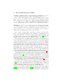
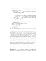
Fig. 1: The single-threaded refinement-checking algorithm where: S is the normalised specification GLTS; I is the implementation GLTS; M is the denotational model to perform the check in; root(X ) returns the root of the GLTS X ;
transitions(X , s) returns the set of all (e, s 0 ) such that there is a transition from
s to s 0 in the GLTS X labelled by the event e; transitions(X , s, e) returns only
successors under event e.
orems of digitisation [17]. In order to support this, FDR3 also supports the prioritise operator [3,18], which has other interesting applications as shown there.
4
Parallel Refinement Checking
We now describe the new multi-core refinement-checking algorithm that FDR3
uses to decide if a normalised GLTS P (recall that normalisation produces a
GLTS with no τ ’s and such that for each state and each event, there is a unique
successor state) is refined by another GLTS Q. We begin by outlining the refinement checking algorithm of [2] and describing the FDR2 implementation [19].
We then define the parallel refinement-checking algorithm, before contrasting our
approach with the approaches taken by others to parallelise similar problems.
In this paper we concentrate on parallelising refinement checking on sharedmemory systems. We also concentrate on refinement checking in models that do
not consider divergence: we will report separately on parallelising this.
The Single-Threaded Algorithm Refinement checking proceeds by performing a
search over the implementation, checking that every reachable state is compatible
with every state of the specification after the same trace. A breadth-first search
is performed since this produces a minimal counterexample when the check fails.
The single threaded algorithm [2,19] is given in Figure 1.
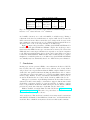
function Worker(S , I , M, w )
donew , currentw , nextw ← {}, {}, {}
finishedw ← true
if hash(root(S ), root(I )) = w then
currentw ← {(root(S ), root(I ))}
finishedw ← false
while ∨w ∈Workers ¬finishedw do
Wait for other workers to ensure the plys start together
finishedw ← true
for (s, i) ← currentw \ donew do
finishedw ← false
Check if i refines s according to M
donew ← donew ∪ {(s, i)}
for (i 0 , e) ∈ transitions(I , i) do
if e = τ then w 0 ← hash(s, i 0 ) mod #Workers
nextw 0 ← nextw 0 ∪ {(s, i 0 )}
else t ← transitions(S , s, e)
if t = {} then Report Trace Error
else {s 0 } ← t
w 0 ← hash(s 0 , i 0 ) mod #Workers
nextw 0 ← nextw 0 ∪ {(s 0 , i 0 )}
Wait for other workers to finish their ply
currentw ← nextw
nextw ← {}
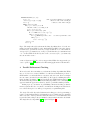
Fig. 2: Each worker in a parallel refinement check executes the above function.
The set of all workers is given by Workers. Hash(s, i ) is an efficient hash function
on the state pair (s, i ). All other functions are as per Figure 1.
The interesting aspect of an implementation of the above algorithm is how
it stores the sets of states (i.e. current, next and done). FDR2 uses B-Trees for
all of the above sets [19], primarily because this allowed checks to efficiently use
disk-based storage when RAM was exhausted (in contrast to, e.g. hash tables,
where performance often decays to the point of being unusable once RAM has
been exhausted). This brings the additional benefit that inserts into done (from
current) can be performed in sorted order. Since B-Trees perform almost optimally under such workloads, this makes insertions into the done tree highly
efficient. To improve efficiency, inserts into the next tree are buffered, with the
buffer being sorted before insertion. The storage that the B-Tree uses is also
compressed, typically resulting in memory requirements being halved.
Parallelisation Parallelising FDR3’s refinement checking essentially reduces to
parallelising the breadth-first search of Figure 1. Our algorithm partitions the
state space based on a hash function on the node pairs. Each worker is assigned
a partition and has local current, next and done sets. When a worker visits
a transition, it computes the worker who is responsible for the destination by
hashing the new state pair. This algorithm is presented in Figure 2.
Whilst the abstract algorithm is straightforward, the implementation has to
be carefully designed in order to obtain good performance. As before, our primary consideration is minimising memory usage. In fact, this becomes even more
critical in the parallel setting since memory will be consumed at a far greater
rate: with 16 cores, FDR3 can visit up to 7 billion states per hour consuming
70GB of storage. Thus, we need to allow checks to exceed the size of the available
RAM. Given the above, B-Trees are a natural choice for storing the sets.
All access to the done and current B-Trees is restricted to the worker who
owns those B-Trees, meaning that there are no threading issues to consider. The
next B-Trees are more problematic: workers can generate node pairs for other
workers. Thus, we need to provide some way of accessing the next B-Trees of
other workers in a thread-safe manner. Given the volume of data that needs to
be put into next (which can be an order of magnitude greater than the volume
put into done), locking the tree is undesirable. One option would be to use finegrained locking on the B-Tree, however this is difficult to implement efficiently.
Instead of using complex locks, we have generalised the buffering that is used
to insert into next under the single-threaded algorithm. Each worker w has a set
of buffers, one for each other worker, and a list of buffers it has received from
other workers that require insertion into this worker’s next. When a buffer of
worker w for worker w 0 6= w fills up, it immediately passes it to the target worker.
Workers periodically check the stack of pending buffers to be flushed, and when
a certain size is exceeded, they perform a bulk insert into next by performing a
n-way merge of all of the pending buffers to produce a single sorted buffer.
One potential issue this algorithm could suffer from is uneven distribution
amongst the workers. We have not observed this problem: the workers have
terminated at roughly the same time. If necessary this could be addressed by
increasing the number of partitions, with workers picking a partition to work on.
We give experimental results that show the algorithm is able to achieve a
near linear speed up in Section 6.
Related Work There have been many algorithms proposed for parallelising BFS,
e.g. [20,21,22,23]. In general, these solutions do not attempt to optimise memory
usage of performance once RAM has been exhausted to the same degree.
The authors of [20] parallelised the FDR2 refinement checker for cluster systems that used MPI. The algorithm they used was similar to our algorithm in
that nodes were partitioned amongst the workers and that B-Trees were used
for storage. The main difference comes from the communication of next: in their
approach this was deferred until the end of each round where a bulk exchange
was done, whereas in our model we use a complex buffer system.
The authors of [21] propose a solution that is optimised for performing a
BFS on sparse graphs. This uses a novel tree structure to efficiently (in terms
of time) store the bag of nodes that are to be visited on the next ply. This was
not suitable for FDR since it does not provide a general solution for eliminating
duplicates in next, which would cause FDR3 to use vastly more memory.
The author of [23] enhances the Spin Model Checker [9] to support parallel
BFS. In this solution, which is based on [24], done is a lock-free hash-table and is
shared between all of the workers, whilst new states are randomly assigned to a
number of subsets which are lock-free linked lists. This approach is not suitable
for FDR since hash-tables are known not to perform well once RAM has been
exhausted (due to their essentially random access pattern). Storing next in a
series of linked-lists is suitable for Spin since it can efficiently check if a node is
in done using the lock-free hash-table. This is not the case for FDR, since there
is no way of efficiently checking if a node is in the done B-Tree of a worker.
5
Compiler
As outlined in Section 3, the compiler is responsible for converting syntactic
processes into GLTSs. This is a difficult problem due to the generality of CSP
since operators can be combined in almost arbitrary ways. In order to allow the
processes to be represented efficiently, FDR3 has a number of different GLTS
types as described in Section 5.1, and a number of different way of constructing each GLTS, as described in Section 5.2. In Section 5.3 we detail the new
algorithm that the compiler uses to decide which of FDR3’s representations of
GLTSs to use. This is of critical importance: if FDR3 were to choose the wrong
representation this could cause the time to check a property and the memory
requirements to greatly increase.
5.1
GLTSs
FDR3 has two main representations of GLTSs: Explicit and Super-Combinator machines. Explicit machines require memory proportional to the number of states
and transitions during a refinement check. In contrast, Super-Combinator machines only require storage proportional to the number of states, since the transitions can be computed on-the-fly. Equally, it takes longer to calculate the transitions of a Super-Combinator machine than the corresponding Explicit machine.
An Explicit GLTS is simply a standard graph data structure. Nodes in an
Explicit GLTS are process states whilst the transitions are stored in a sorted list.
A Super-Combinator machine represents the LTS by a series of component LTSs
along with a list of rules to combine the transitions of the components. Nodes
for a Super-Combinator machine are tuples, with one entry for each component
machine. For example, a Super-Combinator for P ||| Q consists of the components
hP , Qi and the rules:
{(h1 7→ ai, a) | a ∈ αP ∪ {τ }} ∪ {(h2 7→ ai, a) | a ∈ αQ ∪ {τ }}
where αX is the alphabet of the process X (i.e. the set of events it can perform).
These rules describe how to combine the actions of P and Q into actions of the
whole machine. A single rule is of the form (f , e) where f is a partial function
from the index of a component machine (e.g. in the above example, 1 represents
P ) to the event that component must perform. e is the event the overall machine
performs if all components perform their required events.
Rules can also be split into formats, which are sets of rules. For example, a
Super-Combinator for P ; Q would start in format 1 , which has the rules:
{(h1 7→ ai, a, 1) | a ∈ αP ∪ {τ }, a 6= X} ∪ {(h1 7→ Xi, τ, 2) | a ∈ αQ ∪ {τ }}.
The second format has the rules: {(h2 7→ ai, a, 2 ) | a ∈ αQ ∪ {τ }}. Thus, the
first format allows P to perform visible events and stay in format 1 (as indicated
by the third element of the tuple), but if P performs a X and terminates, the
second format is started which allows Q to perform visible events.
Rules can also specify that component machines should be restarted. For
example, to represent P = X ; P as a Super-Combinator, there needs to be a
way of restarting the process X after a X. Thus, we add to the rules a list of
components whose states should be discarded and replaced by their root states:
{({1 7→ a}, a, 1, hi) | a ∈ αX ∪ {τ }, a 6= X)} ∪ {({1 7→ X}, τ, 1, h1i)}.
The first rule set allows X to perform non-X events as usual. However, if X ever
performs a X this is converted into a τ and component 1 (i.e. X ) is restarted.
FDR also recursively combines the rules for Super-Combinator machines. For
example, (P ||| Q) ||| R is not represented as two different Super-Combinator
machines, but instead the rules for P ||| Q and · ||| R are combined. This
process is known as supercompilation. As you might expect from the name, supercombinators are closely related to combinator operational semantics: the “super”
essentially co-incides with the joining together using supercompilation.
5.2
Strategies
There are several different strategies that FDR3 can use to construct Explicit or
Super-Combinator machines from syntactic processes. These strategies differ in
the type of processes that they can support (e.g. some cannot support recursive
processes), the time they take to execute and the type of the resulting GLTS.
The low-level is the simplest strategy and supports any process. An Explicit
LTS is constructed simply by directly applying CSP’s operational semantics.
The high-level compiles a process to a Super-Combinator. This is not able to
compile recursive processes, such as P =
b a → P . The supercombinator rules are
directly constructed using the operational semantics of CSP.
The mixed-level is a hybrid of the low and high-level strategies where, intuitively, non-recursive parts of processes are compiled as per the high-level
strategy whilst recursive parts are compiled as per the low-level strategy. For
example, consider P =
b a → P 2 b → (X ||| Y ): compiling X ||| Y at the
high-level is preferable since it does not require the cartesian product of X
and Y to be formed. If P is compiled at the mixed-level, X ||| Y is compiled
at the high-level, and a → P 2 b → · is compiled into an Explicit machine.
These are wrapped in a Super-Combinator machine that starts X ||| Y when
the Explicit machine performs the b. The supercombinator has two formats,
the first with the rules: {({1 7→ a}, a, 1 ), ({1 7→ b}, b, 2 )} and the second with:
{({2 7→ a}, a, 2 ) | a ∈ α(X ||| Y ) ∪ {τ }}. Thus, when the first process performs
b, the Super-Combinator moves to the second format in which X ||| Y is run.
The next section formalises the set of process that can be compiled in this way.
The recursive high-level strategy is new in FDR3. This compiles to a SuperCombinator machine and allows some recursive processes (which we formalise
in the next section) to be compiled. This is used to compile processes such as
P =
b (X ||| Y ) ; P which are recursive, but are desirable to compile to SuperCombinator machines for efficiency reasons (as above, constructing X ||| Y is
expensive). In this particular case, X ||| Y is compiled to a Super-Combinator
machine, and then a recursive supercombinator is constructed with the rules:
{({1 7→ a}, a, 1, hi) | a ∈ α(X ||| Y ) ∪ {τ }, a 6= X)} ∪ {({1 7→ X}, τ, 1, h1i)}.
Recall that the last component in the above rules indicates that component 1
should be reset. Thus, the above rules indicate that X ||| Y can perform non-X
events normally, but a X will cause X ||| Y to be reset to its initial state.
The majority of processes can be compiled at the recursive high-level, with
the exception of those that recurse through an on argument of an operator (e.g.
P = a → P 2 b → P ). For example, consider the process P = X ; (P 2 . . .):
since 2 is not discarded by a τ , it follows that this recursion is safe only when
X always performs a visible event before a X (otherwise there would be an
infinite series of 2’s applied). This cannot be determined statically (i.e. without
accessing the transitions of X ), and thus it is not possible to determine if the
process can be compiled at the recursive high-level. Thankfully, such processes
are sufficiently rare in the context where recursive high-level is of use.
5.3
Picking a Strategy
We now describe the new algorithm that FDR3 uses to decide how to compile a
syntactic process. The input to the compilation algorithm is a syntactic process
environment (Definition 1) and the output is a list of strategies that specify
how each syntactic processes should be compiled. The algorithm guarantees to
produce a strategy such that executing the strategy yields a valid GLTS that
corresponds to the input process. The algorithm also uses heuristics to attempt
to reduce the time and memory usage during the subsequent refinement check.
All operators have a preferred level of compilation, either low (indicating
Explicit is preferred) or high (indicating Super-Combinator is preferred). For example, prefix prefers the low whilst interleave prefers high. In general, FDR3
aims to compile an operator at its preferred level. If this is high, this may require
using the mixed and recursive high-level strategies on surrounding processes (a
preference for high is more important). When this is not possible (because, e.g.,
the processes do not permit the mixed level), the low-level strategy is used.
The first step is to calculate the strongly connected components (SCCs) of recursive processes. This is done by performing a DFS on the recursion graph that
is naturally formed from the syntactic process environment. Then, we compute
which SCCs can be compiled at the recursive high-level, and which SCCs would
prefer to be compiled at the recursive high-level (by incorporating preferences,
function Strategy(P , r )
. P is a syntactic process, r is an event type
as ← hi
. The strategy for each argument of P
for each argument Q of P do
forceLow ← false
. Set to true if this must be compiled at low
if Q is an on argument of P then
r 0 ← r u discards(P , Q)
forceLow ← r = None
else
. Q is off
if r u turnedOnBy(P , Q) = None then . This might get turned on by
forceLow ← true
. an event that does not discard the context
else r 0 ← Any
. The context is discarded when Q is turned on
if forceLow then as ← as _hLow i
else as ← as _hStrategy(Q, r 0 )i
V
allLow ← a∈as a = Low
if (P is recursive ∨ r 6= Any) ∧ recursionType(P ) 6= High then
if allLow then return Low
else return Mixed
else if P is recursive then return RecursiveHigh
else if P prefers Low then
if allLow then return Low
else return Mixed
else return High
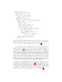
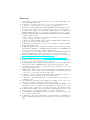
Fig. 3: The algorithm FDR3 uses to decide how to compile syntactic processes.
e.g. prefix prefers to recurse at low, but ; prefers high). The graph is also used to
check for invalid processes, such as P = P 2 P : formally, for each process name
P we check that on each path back to P , at least one off argument is traversed.
Using the recursion graph, FDR3 computes which strategy to use to compile
a syntactic process P . This cannot be done in ignorance of the context of P ,
since this may dictate how a process is compiled. For example, P = a → P 2 Q
requires Q to be compiled at the low-level, since P is a low-level recursion and Q
appears as an on argument of an operator that is on the recursion path. Thus,
when compiling a syntactic process, we need to be aware of the surrounding
context C [·], (e.g. C1 [X ] =
b X ||| STOP ). When deciding on the strategy for P ,
the relevant fact about the context is what events P can perform to cause the
context to be discarded. For example, nothing can discard the context C1 , whilst
any visible event discards the context C2 [X ] =
b X 2 STOP . As we are interested
in statically analysing processes, we approximate these sets as follows.
Definition 2. An event type is either None, Invisible, Visible or Any. The
relation < is defined as None < Invisible, None < Visible, Invisible < Any,
Visible < Any. Note < is a partial order on event types. The meet of e1 and e2
is denoted by e1 u e2 .
Definition 3. Let Q be an argument of a syntactic process P . If Q is on,
then discards(P , Q) returns the event type that Q performs to cause P to be
discarded and Q to be left running (e.g. discards(X 2 Y , X ) = Visible, whilst
discards(X ||| Y , X ) = None). If Q is off , then turnedOnBy(P , Q) returns the
event type that P performs in order to turn on Q. For example, turnedOnBy(X ;
Y , Y ) = Invisible whilst turnedOnBy(X Θ· Y , Y ) = Visible.
Thus it is possible to use discards along with the meet on event types to
compute when a context will be discarded.
Figure 3 defines a function Strategy(P , r ) that returns the strategy that
should be used to compile the syntactic process P in a context that is discarded
by events of event type r . Informally, given a process P and an event type r
this firstly recursively visits each of its arguments, passing down an appropriate event restriction (which is computed using discards for on arguments and
turnedOnBy for off arguments). It may also force some arguments to be low-level
if the restriction becomes None. Then, a compilation strategy for P is computed
by considering the preferences of the operator, whether the operator is recursive and the deduced strategies for the arguments. The overriding observation
behind this choice is that compilation at high is only allowed when the process
is non-recursive, and when there is no surrounding context (i.e. r = Anything).
5.4
Related Work
FDR2 has support for Explicit and Super-Combinator GLTSs, along with a GLTS
definition for each CSP operator (e.g. external choice etc). We believe that the
FDR3 representation is superior, since it requires fewer GLTS types to be maintained and because it makes the GLTSs independent of CSP, making other process algebras easier to support. As mentioned in Section 5.2, FDR2 did not make
use of the recursive high-level, and was unable to automatically compile processes
such as P = (X ||| Y ) ; P at the high-level. We have found that the recursive
high-level has dramatically decreased compilation time on many examples.
The biggest difference is in the algorithm that each uses to compile syntactic processes. FDR2 essentially used a series of heuristics to accomplish this and
would always start trying to compile the process at its preferred level, backtracking where necessary. This produced undesirable behaviour on certain processes.
We believe that since the new algorithm is based on the operational semantics of
CSP, it is simpler and can be easily applied to other CSP-like process algebras.
6
Experiments
We compare the performance of a pre-release version of FDR 3.1.0 to FDR 2.94,
Spin 6.25, DiVinE 3.1 beta 1, and LTSmin 2.0, on a complete traversal of a
graph. The experiments were performed on a Linux server with two 8 core 2GHz
Xeons with hyperthreading (i.e. 32 virtual cores), 128GB RAM, and five 100GB
SSDs. All input files are available from the first author’s webpage. — denotes a
check that took over 6 hours, * denotes a check that was not attempted, and †
denotes a check that could not be completed due to insufficient memory. Times
Input
bully.7
cuberoll.0
ddb.0
knightex.5.5
knightex.3.11
phils.10
solitare.0
solitare.1
solitaire.2
tnonblock.7
States Transitions
Time
(10 6 )
(10 6 )
FDR2
129
1354
2205 (4.8)
7524
20065
—
65
377
722 (1.4)
67
259
550 (1.4)
19835
67321
*
60
533
789 (1.3)
187
1487
2059 (4.4)
1564
13971
19318 (35.1)
11622 113767
*
322
635
2773 (6.7)
(s) & Storage (GB)
FDR3-32
FDR3-1
FDR3-32 Speedup
1023 (2.2)
85 (5.5)
12.0
—
3546 (74.5)
—
405 (0.5)
31 (2.36)
13.1
282 (0.6)
23 (2.4)
12.3
*
26235 (298.5)
—
431 (0.5)
32 (2.0)
13.5
1249 (1.6)
84 (3.8)
14.9
11357 (11.7) 944 (17.5)
12.0
*
9422 (113.3)
—
937 (2.6)
109 (6.8)
8.6
15
Speedup
10
5
bully.7
solitaire.0
tnonblock.7
0
0
10
20
Workers
30
(b) FDR3’s scaling performance.
Millions of States per Second
(a) Times comparing FDR2, FDR3 with 1 worker, and FDR3 with 32 workers.
Memory exceeded
2
1
0
0
1
Time (s)
2
·10 4
(c) Disk storage performance on knightex.3.11.
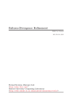
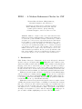
Fig. 4: Experimental results demonstrating FDR3’s performance.
refer to the total time required to run each program whilst memory figures refer
to the maximum Resident Set Size plus any on-disk storage used.
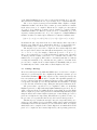
Figure 4a compares the performance of FDR2 and FDR3. FDR3 with 1
worker substantially outperforms FDR2. This is because FDR3’s B-Tree has been
heavily optimised and because FDR3 makes fewer allocations during refinement
checks. FDR3 with 1 worker also uses less memory than FDR2: this is due to a
new compaction algorithm used to compress B-Tree blocks that only stores the
difference between keys. The extra memory used for the parallel version is for
extra buffers and the fact that the B-Tree blocks do not compress as well.
The speed-ups that Figures 4a and 4b exhibit between 1 and 32 workers vary
according to the problem. solitaire is sped up by a factor of 15 which is almost
optimal given the 16 cores. Conversely, tnonblock.7 is only sped up by a factor
of 9 because it has many small plys, meaning that the time spent waiting for
other workers at the end of a ply is larger.
Figure 4c shows how the speed that FDR3 visits states at changes during
the course of verifying knightex.3.11, which required 300GB of storage (FDR3
Input
knightex.5.5
knightex.3.10
knightex.3.11
solitaire.0
Time (s) & Storage (GB)
Spin-32
FDR3-32 DiVinE-32 LTSmin-32
12 (5.8)
23 (2.4)
13 (4.6) 28 (33.1)
396 (115.0) 943 (22.7)
†
395 (35.5)
†
26235 (298.5)
†
†
89 (15.5)
85 (3.9)
85 (14.3) 73 (36.4)
Fig. 5: A comparison between FDR3, Spin, DiVinE and LTSmin. knightex.3.10
has 2035 × 10 6 states and 6786 × 10 6 transitions.
used 110GB of memory as a cache and 190GB of on-disk storage). During a
refinement check, the rate at which states are explored will decrease because the
B-Trees increase in size. Observe that there is no change in the decrease of the
state visiting rate after memory is exceeded. This demonstrates that B-Trees are
effectively able to scale to use large amounts of on-disk storage.
Figure 5 compares the performance of FDR3, Spin, DiVinE and LTSmin. For
in-memory checks Spin, DiVinE and LTSmin complete the checks up to three
times faster than FDR3 but use up to four times more memory. We believe that
FDR3 is slower because supercombinators are expensive to execute in comparison
to the LTS representations that other tools use, and because B-Trees are slower
to insert into than hashtables. FDR3 was the only tool that was able to complete
knightex.3.11 which requires use of on-disk storage; Spin, DiVinE and LTSmin
were initially fast, but dramatically slowed once main memory was exhausted.
7
Conclusions
In this paper we have presented FDR3, a new refinement checker for CSP. We
have described the new compiler that is more efficient, more clearly defined
and produces better representations than the FDR2 compiler. Further, we have
detailed the new parallel refinement-checking algorithm that is able to achieve
a near-linear speed-up as the number of cores increases whilst ensuring efficient
memory usage. Further, we have demonstrated that FDR3 is able to scale to
enormous checks that far exceed the bounds of memory, unlike related tools.
This paper concentrates on parallelising refinement checks on shared-memory
systems. It would be interesting to extend this to support clusters instead: this
would allow even larger checks to be run. It would also be useful to consider
how to best parallelise checks in the failures-divergence model. This is a difficult
problem, in general, since this uses a depth-first search to find cycles.
FDR3 is available for 64-bit Linux and Mac OS X from https://www.cs.
ox.ac.uk/projects/fdr/. FDR3 is free for personal use or academic research,
whilst commercial use requires a licence.
Acknowledgements This work has benefitted from many useful conversations
with Michael Goldsmith, Colin O’Halloran, Gavin Lowe, and Nick Moffat. We
would also like to thank the anonymous reviewers for their useful comments.
References
1. C. A. R. Hoare, Communicating Sequential Processes. Upper Saddle River, NJ,
USA: Prentice-Hall, Inc., 1985.
2. A. W. Roscoe, The Theory and Practice of Concurrency. Prentice Hall, 1997.
3. A. W. Roscoe, Understanding Concurrent Systems. Springer, 2010.
4. J. Lawrence, “Practical Application of CSP and FDR to Software Design,” in Communicating Sequential Processes. The First 25 Years, vol. 3525 of LNCS, 2005.
5. A. Mota and A. Sampaio, “Model-checking CSP-Z: strategy, tool support and
industrial application,” Science of Computer Programming, vol. 40, no. 1, 2001.
6. C. Fischer and H. Wehrheim, “Model-Checking CSP-OZ Specifications with FDR,”
in IFM’99, Springer, 1999.
7. G. Lowe, “Casper: A Compiler for the Analysis of Security Protocols,” Journal of
Computer Security, vol. 6, no. 1-2, 1998.
8. A. W. Roscoe and D. Hopkins, “SVA, a Tool for Analysing Shared-Variable Programs,” in Proceedings of AVoCS 2007, 2007.
9. G. Holzmann, Spin Model Checker: The Primer and Reference Manual. AddisonWesley Professional, 2003.
10. J. Barnat, L. Brim, V. Havel, J. Havlíček, J. Kriho, M. Lenčo, P. Ročkai, V. Štill,
and J. Weiser, “DiVinE 3.0 – An Explicit-State Model Checker for Multithreaded
C & C++ Programs,” in CAV, vol. 8044 of LNCS, 2013.
11. A. Laarman, J. v. d. Pol, and M. Weber, “Multi-Core LTSmin: Marrying Modularity and Scalability,” in NASA Formal Methods, vol. 6617 of LNCS, 2011.
12. University of Oxford, Failures-Divergence Refinement—FDR 3 User Manual, 2013.
https://www.cs.ox.ac.uk/projects/fdr/manual/.
13. University of Oxford, libcspm, 2013. https://github.com/tomgr/libcspm.
14. G. M. Reed and A. W. Roscoe, “A Timed Model for Communicating Sequential
Processes,” Theoretical Computer Science, vol. 58, 1988.
15. P. Armstrong, G. Lowe, J. Ouaknine, and A. W. Roscoe, “Model checking Timed
CSP,” In Proceedings of HOWARD (Festschrift for Howard Barringer), 2012.
16. J. Ouaknine, Discrete Analysis of Continuous Behaviour in Real-Time Concurrent
Systems. DPhil Thesis, 2001.
17. H. Barringer, R. Kuiper, and A. Pnueli, “A really abstract concurrent model and its
temporal logic,” in Proceedings of the 13th ACM SIGACT-SIGPLAN symposium
on Principles of programming languages, ACM, 1986.
18. A. W. Roscoe and P. J. Hopcroft, “Slow abstraction via priority,” in Theories of
Programming and Formal Methods, vol. 8051 of LNCS, 2013.
19. A. W. Roscoe, “Model-Checking CSP,” A Classical Mind: Essays in Honour of
CAR Hoare, 1994.
20. M. Goldsmith and J. Martin, “The parallelisation of FDR,” in Proceedings of the
Workshop on Parallel and Distributed Model Checking, 2002.
21. C. E. Leiserson and T. B. Schardl, “A work-efficient parallel breadth-first search
algorithm (or how to cope with the nondeterminism of reducers),” in Proc. 22nd
ACM symposium on Parallelism in algorithms and architectures, SPAA ’10, 2010.
22. R. E. Korf and P. Schultze, “Large-scale parallel breadth-first search,” in Proc. 20th
national conference on Artificial intelligence - Volume 3, AAAI, 2005.
23. G. J. Holzmann, “Parallelizing the Spin Model Checker,” in Model Checking Software, vol. 7385 of LNCS, 2012.
24. A. Laarman, J. van de Pol, and M. Weber, “Boosting multi-core reachability performance with shared hash tables,” in Formal Methods in Computer-Aided Design,
2010.