1
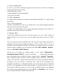
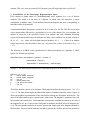
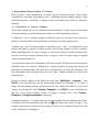
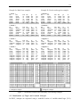
DIAV 2.0 User Manual Specification and Guide through the Diagrammatic Visualization System Janusz Wnek Machine Learning and Inference Laboratory George Mason Univesity 4400 University Dr., Fairfax, VA 22030 [email protected] Tue, N ov 21, 1995 2 Table of Contents 1. INTRODUCTION . . . . . . . . . . . . . . . . . . . . . . . . . . . . . . . . . . . . . . . . . . . . . . . . . . . . . . . . . . . . . . . . . . . . . . . . . . . . . . . . . . . . . . . . . 3 2. GETTING STARTED. . . . . . . . . . . . . . . . . . . . . . . . . . . . . . . . . . . . . . . . . . . . . . . . . . . . . . . . . . . . . . . . . . . . . . . . . . . . . . . . . . . . . 4 2.1 SYSTEM REQUIREMENTS ..................................................................................................................5 2.2 DIAV DISTRIBUTION .......................................................................................................................5 2.3 RUNNING DIAV...............................................................................................................................5 2.4 TEXT EDITING .................................................................................................................................6 2.5 TAKING A SNAPSHOT OF THE DIAV SCREEN ........................................................................................6 2.6 EXITING DIAV ................................................................................................................................6 3. VISUALIZATION OF THE KNOWLEDGE REPRESENTATION SPACE . . . . . . . . . . . . . . . . . . . . . . 7 4. DIAGRAMMATIC REPRESENTATION OF CONCEPTS . . . . . . . . . . . . . . . . . . . . . . . . . . . . . . . . . . . . . . . . . 9 4.1 VISUALIZATION OF TRAINING EXAMPLES............................................................................................9 4.2 VISUALIZATION OF TARGET AND LEARNED CONCEPTS ........................................................................ 10 4.3 CONCEPT CONSTRUCTION .............................................................................................................. 13 5. CHANGING THE REPRESENTATION SPACE. . . . . . . . . . . . . . . . . . . . . . . . . . . . . . . . . . . . . . . . . . . . . . . . . . . . 2 0 5.1 CONTRACTION .............................................................................................................................. 20 5.2 EXPANSION .................................................................................................................................. 23 6. DEMO: STAR GENERATION. . . . . . . . . . . . . . . . . . . . . . . . . . . . . . . . . . . . . . . . . . . . . . . . . . . . . . . . . . . . . . . . . . . . . . . . . 2 6 7. SIMPLE SESSION WITH DIAV 2.0 . . . . . . . . . . . . . . . . . . . . . . . . . . . . . . . . . . . . . . . . . . . . . . . . . . . . . . . . . . . . . . . . . 3 3 8. DIAV SYSTEM MENUS . . . . . . . . . . . . . . . . . . . . . . . . . . . . . . . . . . . . . . . . . . . . . . . . . . . . . . . . . . . . . . . . . . . . . . . . . . . . . . . 3 5 9. DIAV SYNTAX . . . . . . . . . . . . . . . . . . . . . . . . . . . . . . . . . . . . . . . . . . . . . . . . . . . . . . . . . . . . . . . . . . . . . . . . . . . . . . . . . . . . . . . . . . 3 8 10. DIAV DATA STRUCTURES. . . . . . . . . . . . . . . . . . . . . . . . . . . . . . . . . . . . . . . . . . . . . . . . . . . . . . . . . . . . . . . . . . . . . . . . . 4 1 REFERENCES. . . . . . . . . . . . . . . . . . . . . . . . . . . . . . . . . . . . . . . . . . . . . . . . . . . . . . . . . . . . . . . . . . . . . . . . . . . . . . . . . . . . . . . . . . . . . . . 4 2 3 Abstract The goal of the diagrammatic visualization system DIAV is to provide a tool for a visual interpretation of various aspects of concept learning. These include: visualization of knowledge representation spaces and relationships between training examples and target and learned concepts, and visual comparison of knowledge transmutations performed by various learning systems, e.g. visualization of changes in the representation space done by constructive induction. The system employs a planar model of a multidimensional space spanned over a set of discrete attributes. The model is in the form of a diagram, in which each cell represents a unique combination of attribute values. The diagram can represent examples, rules, and rulesets (DNF) in the form of concept images. The system is very useful for analyzing behavior of existing learning algorithms and in every stage of development of a new learning system. 1. Introduction The diagrammatic visualization system DIAV employs a planar model of a multidimensional space spanned over a set of discrete attributes. The model is called General Logic Diagram (GLD) and was introduced by Michalski in 1978. The model is in the form of a diagram, in which each cell represents a unique combination of attribute values. Each attribute partitions the diagram into areas corresponding to individual values of the attribute. Conjunctive rules correspond to certain regular arrangements of cells that can be easily recognized visually. The diagram can represent examples, rules, and rulesets (DNF) in the form of concept images. The main goal of the diagrammatic visualization system DIAV is to provide a tool for a visual interpretation of various aspects of concept learning. These include: visualization of knowledge representation spaces and relationships between training examples and target and learned concepts (Wnek et. al. 1990); visual comparison of generalization performed by various learning systems (Wnek et al. 1990, Wnek and Michalski, 1994a); visualization of changes in the representation space done by constructive induction (Wnek, 1993; Wnek & Michalski, 1994b). An important feature of the diagrammatic visualization is that it permits one to display steps in learning processes as well as the errors in concept learning. The set of cells representing the target concept (the concept to be learned) is called target concept image (T). The set of cells representing the learned concept is called learned concept image (L). The areas of the target concept not covered by the learned concept represent errors of omission (T \ L), while the areas of the learned concept not covered by the target concept represent errors of commission (L \ T). The union of both types of errors represents the error image. The system can also display results of any operation on the concept, such as generalization, specification, or any change of the description space, such as adding or deleting attributes, or their values. Another interesting feature is that it can also visualize concepts acquired by non-symbolic systems, such as neural nets or genetic algorithms. Using the diagram one can express the learned concepts in the form of decision rules. Thus, the diagram allows one to evaluate both the quality and the rule-complexity of the results of symbolic and non-symbolic learning. The implemented 4 system, DIAV, can display description spaces up to 4M events, i.e., spaces spanned over up to 22 binary variables (or correspondingly smaller number of multiple-valued variables). The system is very useful for analyzing behavior of existing learning algorithms and in every stage of development of a new learning system. Following are the features implemented in the current version of the system DIAV 2.0: 1. The maximum event space (ES) size for a direct display is 4 M events (22 binary attributes), and for a virtual display is 32 M events (25 binary attributes) on a workstation with 8 MB memory. 2. System is window and menu driven. An input to the system comes from a graphical terminal and from data files generated within the system or generated by a learning system (e.g. AQ15). Output is directed to a graphical terminal with regards to visual effects, and to data files for communication with a learning system or for a further use by DIAV. The graphical terminal is able to display and control multiple windows. Windows are furnished with standard control boxes for zooming in and out the window. Scroll bars on sides of the panes enable to display larger then screen size images and to have an convenient character input/output. DIAV inherits all standard Smalltalk/V features. A user can take advantage of, for instance, built-in text editor, cut/copy/paste feature, or font chooser (see Appendix A - DIAV system menus). 3. The DIAV 2.0 system enables: • Visualization of target and learned concepts • Visualization of arbitrary rules either by specifying their description or by direct drawing • Visualization of errors of commission, omission and the complete error image • Construction of complex concepts by using AND, OR, DIFF, NOT, and XOR operators • Projection of a given representation space into another one by removing and/or adding attributes 4. Future features of the DIAV system will include the following AQ-specific operators: • operator refunion • extension against (EA) • square-root (the set of all maximal complexes inside the set • star-of-event ( SR ( EA( e, NegEvents ))) 2. Getting Started 5 2.1 System Requirements In order to use the DIAV visualization program (hereafter referred to as DIAV), the following system requirements must be satisfied: • Macintosh System 7 or later. • Installed Smalltalk/V Mac from Digitalk Inc. • At least 2M of free RAM. 2.2 DIAV Distribution The complete DIAV distribution is provided on a single diskette entitled DIAV 2.0, which contains the following: • DIAV - the DIAV application. • ReadMe - the ReadMe text file. Be sure to read this file as it may contain important information and instructions not provided in this manual. • Example - the Example folder with an example knowledge representation space (Robots.rs), target and learned concepts (Robots.tc1, Robots.lc1) 2.3 Running DIAV To start DIAV, double-click on its icon to open the program. You can use DIAV without any additional setting. If you wish, however, you can change default font style from the Window menu. DIAV is run under the control of Smalltalk/V Mac. This way, DIAV inherits whole functionality of Smalltalk/V, allowing for file and string manipulation, as well as window control. It is easy to distinguish between Smalltalk/V and DIAV environments by checking which set of menus is currently available. Smalltalk/V uses the following menus: File Edit Smalltalk Window. DIAV uses: File DIAV.1 DIAV.2 Window. After the start, two windows are displayed (Figure 1). One window, Diagrammatic Visualization System DIAV 2.0 , is used for visualization of knowledge representation spaces. This window comes with the DIAV menus. Another window is System Transcript. This is Smalltalk's window, and when selected, Smalltalk's menus will become available. This window is used by DIAV to display textual information about various transformations performed on diagrams, such as, the number of commission errors, which file the representation space description was read from, etc. Through this window, you can also specify rules to be displayed by DIAV. At the beginning of the System Transcript there is a command: (DIAV new open:" on nil) to open more DIAV-type windows. In order to create an additional window select (highlight) the text of the command, including brackets, and select Do it from Smalltalk menu. This way you can visualize many DIAV windows at the same time. 6 2.4 Text Editing Text editing in DIAV is one of the features inherited from Smalltalk/V. It conforms to text editing conventions of the Macintosh such as, moving the insertion point, deleting/inserting characters, selecting words/lines/text, deselecting text, deleting selected text, cutting/coping/pasting selected text. The File menu contains all commands needed for text exditing and printing. They include, New, Open ..., Save, Save As ..., Revert to Saved, Page Setup, and Print ... . 2.5 Taking a Snapshot of the DIAV Screen In order to make a snapshot of the current screen press the following keys Shift- -3. A "Picture" file will be created in the main folder. You can "cut and paste" a desired segment into your publication. 2.6 Exiting DIAV To exit DIAV and return to the Macintosh OS, select Quit from the File menu. You will be prompted with a dialog box which asks whether or not to save your current environment — a kind of snapshot of all existing objects on your DIAV desktop, including window placement and 7 contents. This way, when you restart DIAV program, you will begin right where you left off. 3. Visualization of the Knowledge Representation Space DIAV employs a planar model of a multidimensional space spanned over a set of discrete attributes. The model is in the form of a diagram, in which each cell represents a unique combination of attribute values. Each attribute partitions the diagram into areas corresponding to individual values of the attribute. A representation space description is assumed to be in a form of a text file. This file has to begin with a domain name followed by a specification of a size of the domain (for every attribute, the number of values has to be specified). If there is no attribute and value definition following, system will assume default names for attributes and their values (attributes can be then referred as x0, x1, x2, ..., xn; values will be default numerical numbers: 0,1,2, ... ). Values of an attribute can be expressed as a list of nominal values (e.g., red, green, blue, yellow) or an interval (e.g., 10 .. 17). The following is an EBNF syntax specification for domain description (see Appendix A. DIAV Syntax, for detailed specification). domainDescription = domainName "(" number { "," number } ")" { attributeName "=" interval | attributeName "=" attributeValue { "," attributeValue } Example 1: The following description of the representation space is in the Robots.rs file. Robots (3, 3, 2, 3, 4, 2) hs = round, square, octagonal bs = round, square, octagonal sm = yes, no ho = sword, balloon, flag jc = red, green, blue, yellow ti = yes, no The Robots domain consists of six attributes. The header line defines the domain space: 3 x 3 x 2 x 3 x 4 x 2. The lines following the headline define names of attributes and their values. Figure 2a shows the graphical representation of this domain after reading the description from the file. The name of the representation space is placed as the window title. The diagram is partitioned into cells by horizontal and vertical lines. Horizontal lines correspond to attributes described on the side of the diagram (hs, bs, sm). Vertical lines correspond to attributes described below the diagram (ho, jc, ti). The most outside attributes (hs and bs) generate the largest grid in the diagram (marked by thickest lines). The most inside attributes (sm and ti) generate the smallest grid and are marked by 8 thinnest lines. The attributes can be rearranged in the diagram by changing their sequence in the file describing the representation space. Each example in the representation space has its unique representation in the diagram. Example 2: Robots (3, 3, 2, 3, 4, 2) Given this domain description, the system will generate the diagram shown in Figure 2b. Please note default attribute names and values. A. Attribute names and values defined by a user. B. Default attribute names and values. Figure 2. Diagrammatic representations of the ROBOTS domain. 9 4. Diagrammatic Representation of Concepts DIAV provides a visual interpretation of various aspects of concept learning. These include: visualization of knowledge representation spaces, relationship between training examples, target and learned concepts, visualization of changes in the representation space done by constructive induction. 4.1 Visualization of Training Examples There can be a number of ways to visualize preclassified examples of many classes. In the context of concept learning, we use the following two modes for visualizing training examples. 1) Multi-class - mode. Training examples of different classes are visualized using consecutive numbers. This mode allows seeing distribution of examples in the representation space. 2) Binary-class - mode. Training examples are visualized using "+" and "-" to distinguish between positive and negative examples. Examples of some classes can be marked as positive examples, and the remaining classes as negative examples. A special case of this type includes situation when one class is selected as positive and other classes as negative. This is a typical strategy in multiple concept learning (Example 3b). A set of training examples for visualization is read from a text file. The file can be created using the Smalltalk's editor (see Section 2.4 Editing Text). Training examples are grouped into classes and represented as relational tables. Each class has to be identified by its name, and followed by the line with attribute names defining their order in the table. Training examples are listed in the following lines. In order to display examples in the multi-class mode select Multiclass examples from DIAV.2 menu, and than select the file with training examples as in Example 3a. In order to dispaly the same training examples in the binary-class mode, change class labels to Positive and Negative as in Example 3b, select Training Examples from DIAV.1 menu, and identify the data file. If you want to display Positive or Negative examples only, select Positive Examples, or Negative Examples, respectively. Ambiguous examples, i.e. examples that have the same attribute values but different class labels, are marked with # in the multi-class mode, and with in the binary-class mode. In Figure 3, the example [hs=square] & [bs=round] & [sm=no] & [ho=flag] & [jc=yellow] & [ti=yes] belongs to both Class1 and Class2, and therefore is ambiguous. 10 Example 3a. Multi-class examples Example 3b. Positive and negative examples ! Class1 ! hs bs round round round square round square square round square round square round sm no no no yes yes no ho sword sword sword sword sword flag jc red red red red red yellow ti yes yes no yes no yes ! Negative ! hs bs round round round square round square square round square round square round sm no no no yes yes no ho sword sword sword sword sword flag jc red red red red red yellow ti yes yes no yes no yes ! Class2 ! hs bs square square square octagonal square square square octagonal square round square round sm yes yes no no yes no ho sword sword sword sword flag flag jc yellow yellow yellow yellow yellow yellow ti no no no no yes yes ! Positive hs square square square square square square ! bs square octagonal square octagonal round round sm yes yes no no yes no ho sword sword sword sword flag flag jc yellow yellow yellow yellow yellow yellow ti no no no no yes yes ! Class3 hs round octagonal round ! bs octagonal octagonal octagonal sm yes yes no ho sword sword sword jc yellow yellow yellow ti yes no yes ! Negative ! hs bs round octagonal octagonal octagonal round octagonal sm yes yes no ho sword sword sword jc yellow yellow yellow ti yes no yes ! Class4 hs round round square square octagonal octagonal octagonal octagonal ! bs octagonal octagonal octagonal octagonal octagonal octagonal octagonal octagonal sm yes yes yes yes yes yes no no ho flag flag flag flag flag flag flag flag jc yellow yellow yellow yellow green green green green ti yes no yes no yes no yes no ! Negative ! hs bs round octagonal round octagonal square octagonal square octagonal octagonal octagonal octagonal octagonal octagonal octagonal octagonal octagonal sm yes yes yes yes yes yes no no ho flag flag flag flag flag flag flag flag jc yellow yellow yellow yellow green green green green ti yes no yes no yes no yes no # - ambiguous example - ambiguous example Figure 3. Visualization of multi-class and binary-class training examples 4.2 Visualization of Target and Learned Concepts In DIAV, concepts are expressed using a modified version of variable-valued logic (VL1) 11 language. A concept can be described using either rules or examples (Figures 4 & 5). The rules consist of conjunctive conditions enclosed in brackets. The rules are separated by semicolons. The conditions relate attribute with their possible values. If the concept is specified using examples, a list of attribute names should appear before the examples to define order of attribute values in the table. The concept representation in the form of rules is useful for symbolic learning systems that produce output of this kind, e.g. AQ15 (Michalski et al, 1986), C4.5 (Quinlan, 1993). For nonsymbolic learning systems, such as, neural networks, genetic algorithms, the concept representation in the form of examples facilitates visualization of results from those systems (Wnek et al., 1989). concept = rule { ";" rule } | listOfAttributeNames example { example } rule = condition { condition } condition = "[" expression "]" expression = attributeName REL attributeValue { "," attributeValue} | attributeName "=" interval REL = "<" | "<=" | interval = attributeValue ".." attributeValue listOfAttributeNames = attributeName { attributeName } example = attributeValue { attributeValue } "=" | "=>" | ">" Figure 4. Concept representation using rules or examples An important feature of DIAV is that it permits displaying steps in concept learning. The set of cells representing the target concept (the concept to be learned) is called target concept image (T). The set of cells representing the learned concept is called learned concept image (L). Concept images are represented in the diagrams by shaded areas. Target concept image is represented by light gray shade, learned concept image is represented by dark gray shade. If the target and learned concepts are both visualized in the same diagram, then their overlap becomes black. One of the three cases may occur. If the learned concept totally matches the target concept then the whole image is black. If there are some areas of the target concept not covered by the learned concept description then these areas reflect errors of omission (light gray area). If the learned area is larger than the target (overgeneralization of the concept), then the dark gray area represents errors of commission (Figure 6). 12 Example 5a. The concept represented as a set of examples hs round round round round round round round round round round round round round round bs square square square square square square square square square square square square square square sm no no no no no no no no no no no no no no ho sword sword sword sword sword sword sword sword flag flag flag flag flag flag jc red green blue yellow red green blue yellow red green blue yellow red green ti yes yes yes yes no no no no yes yes yes yes no no round round octagonal octagonal octagonal octagonal octagonal octagonal octagonal octagonal square square square square square square square square square square no no no no yes yes no no yes yes flag flag balloon balloon balloon balloon balloon balloon balloon balloon blue yellow red green red green red green red green no no yes yes yes yes no no no no Example 5b. The concept represented as a set of rules [hs=round] [bs=square] [sm=no] [ho=sword, flag] ; [hs=octagonal] [bs=square] [ho=balloon] [jc=red, green] Figure 5. Concept visualization from descriptions in the form of examples or rules. 13 A. Target concept image B. Learned concept image C. Target and learned concept image D. Error area image Figure 6. Target and learned concept images and their relationship. 4.3 Concept Construction DIAV enables construction of arbitrary concept images. A concept image is constructed either by direct selection of examples on the screen or by combining current concept image with other concept descriptions using predefined operators such as, AND, OR, DIFF, NOT, and XOR. The direct selection of examples is done by clicking on selected cells in the diagram. Clicking on an empty cell adds the cell into the concept image. Clicking on an cell belonging to the concept image removes the cell from the concept image. The concept image can be combined with another concept by selecting one of the predefined operators and the concept description stored in a file. The concept description can be in the form of rules or examples. 14 The constructed concept image can at any time be transformed into the concept description in the form of positive and negative examples and stored in a file. It can later be used as an input for a learning system. In order to construct a concept image, display a new Representation Space or select Clear Diagram to clear the current one. Next, select Construct a Concept to initialize the concept image by either direct input or visualization of the concept description stored in a file. Next, combine the image with other concept descriptions using the AND, OR, DIFF, NOT, and XOR operators from the DIAV menu. At any time, the concept image can be changed by directly switching on/off concept examples. Figure 7 illustrates application of various operators used in constructing concept images in the Robots representation space. The descriptions of the initial concept A and other concepts (B, D, F , and H) used as operands were stored in separate files. Below are the concept descriptions in the form of rules. A [ho=sword,flag]; [ho=balloon] [hs=square] B [hs=square]; [ho=balloon] [hs=octagonal] [bs=square] D [bs=square] F [ho=balloon] [hs=square]; [ho=flag] [hs=round,octagonal] [bs=round] H [jc=red,blue] The following sequence of commands constructs the images shown in Figure 7. It starts with displaying the initial concept A. This concept image is combined using operator AND with the concept B. The resulting image (concept C) is combined with concept D using operator OR, etc. Construct a Concept AND OR DIFF Input: A Input: A, B Input: C, D Input: E, F Output: A Output: C Output: E Output: G 15 XOR NOT Input: G, H Input: I The following transcript is created in the System Transcript window: Domain description read from file: ...:Constructing concepts:Robots.rs A concept read from file: ...:Constructing concepts:ConstructConcept.a AND concept from file: ...:Constructing concepts:ConstructConcept.b AND OR concept from file: ...:Constructing concepts:ConstructConcept.c OR DIFF concept from file: ...:Constructing concepts:ConstructConcept.d DIFF XOR concept from file: ...:Constructing concepts:ConstructConcept.e XOR NOT Output: I Output: J 16 A B C := A AND B D E := C OR D F Figure 7. Constructing concept images. 17 G := E \ F H I := G XOR H J := NOT I Figure 7 (cont.). Constructing concept images. The following example (Figure 8) shows construction of symmetrical concepts using the XOR operator (Wnek and Michalski, 1994). In the 4-dimensional representation space represented by 4 binary attributes, x0, x1, x2, x3, the initial concept is [x0=0]. Consecutive concepts are created by executing the XOR operation with [x1=0], [x2=0], [x3=0] rules, respectively. The resulting concept D is symmetrical with respect to all four attributes. (It represents the parity concept "odd number of attributes have value 1"). 18 A := [x0=0] B := A xor [x1=0] C := B xor [x2=0] D := C xor [x3=0] Figure 8. Constructing concept images: symmetrical concepts. A concept can be saved in the form of training examples in two formats: one is AQ-type format and second is C4.5 (ID3)-type format. The following commands allow saving the constructed concept: Save Concept AQ and Save Concept C4.5. The examples below show descriptions created for the concept D. Example 5. Examples defining the constructed concept as saved in AQ and C4.5 formats 5a. AQ format 5b. C4.5 format p-events x0 x1 x2 x3 0 0 0 1 0 0 1 0 0 1 0 0 0 1 1 1 1 0 0 0 1 0 1 1 1 1 0 1 1 1 1 0 n-events x0 x1 x2 x3 0 0 0 0 0 0 1 1 0 1 0 1 0 1 1 0 1 0 0 1 1 0 1 0 1 1 0 0 1 1 1 1 x0 x1 x2 x3 0,0,0,1,p 0,0,1,0,p 0,1,0,0,p 0,1,1,1,p 1,0,0,0,p 1,0,1,1,p 1,1,0,1,p 1,1,1,0,p 0,0,0,0,n 0,0,1,1,n 0,1,0,1,n 0,1,1,0,n 1,0,0,1,n 1,0,1,0,n 1,1,0,0,n 1,1,1,1,n The next example (Figure 9) shows symmetry of the Monk2 concept. Diagram A shows a symmetrical concept constructed by performing XOR operation on all first attribute values. Therefore, the diagram shows concept odd(FirstValue(Attribute)). Diagram B shows the Monk2 concept. Diagram C shows the odd(FirstValue(Attribute)) concept in light gray shading and the Monk2 concept in gray shading. There is no intersection between the two. Diagram D shows the negated concept odd(FirstValue(Attribute)) and the Monk2 concept. The black area (intersection of 19 the two concepts) is exactly the Monk2 concept. The negation of odd(FirstValue(Attribute)) is even(FirstValue(Attribute)). Monk2 is a subconcept of even(FirstValue(Attribute)). A. odd(FirstValue(Attribute)) B. Monk2 C. odd(FirstValue(Attribute)) or Monk2 D. even(FirstValue(Attribute)) or Monk2 Figure 9. Constructing concept images: the symmetry of the Monk2 concept. 20 5. Changing the Representation Space The representation space transformations may involve contraction, expansion, or exchange operations. In the context of the attribute-value concept representation, contraction is done by removing attributes, or combining attribute values into larger units. Expansion is done by adding new attributes or by adding new attribute values to the value sets of existing attributes. Exchange is done by replacing original attributes with new ones. All transformations of the representation space are performed using the Project to ... command. DIAV prompts for a new description file, and creates an internal mapping between the representations. A new window with a diagram is created for the new representation space. The diagram is labeled with its predecessor's name followed by semicolon and new domain name read from the description file (e.g. Original_RS:New_RS). Next, by selecting commands, such as Training Examples, Target Concept, etc., DIAV will project examples or concepts from the previous representation space to the new one (instead of reading them form a file). The new representation space description file has similar syntax to the description file of the original representation space. Additional components consist of definitions of new attribute values. Those definitions use original attributes and are in the DNF form (see the DIAV Syntax section). 5.1 Contraction In some situations, there is an interest in displaying an image of a reduced (abstracted) representation space. For example, some constructive induction learning systems reduce knowledge representation spaces to remove redundancy or insignificant attributes (Wnek, 1993; Wnek & Michalski, 1994). The representation space can be reduced either by removing some attributes, or by replacing some attribute values by more general values. Representation space contraction can lead to interesting observations, like finding strong relationships between attributes, or on the other hand, finding irrelevant attributes. The example below, illustrates the two ways of contracting the representation space. We begin with the Robots representation space and four positive and one negative example (Figure 10a). 21 ! Positive ! hs bs octagonal round octagonal round square round round square sm ho jc ti no balloon red yes no balloon green yes no sword red yes yes flag red no ! Negative ! hs bs sm square square yes ho flag jc ti yellow no Figure 10a. Original representation space with 5 training examples. Figure 10b illustrates the representation space contraction by removing the attribute "jc". The new domain description file was created by simply changing the domain name and by removing "jc" attribute description. In the abstracted representation space, some examples from one class may end up having the same description and therefore be placed in the same diagram cell. This operation combined two different examples of the positive class into two equivalent examples. ! Positive ! hs bs octagonal round octagonal round Robots_jc_removed sm no no ho balloon balloon jc red green ti yes yes (3,3,2,3,2) hs = round, square, octagonal bs = round, square, octagonal sm = yes,no ho = sword,balloon,flag ti = yes,no Figure 10b. Contracted representation space by removing an attribute. 22 Figures 10c, 10d illustrate the contraction operation by both removing the attribute "jc" and the attribute value "hs=square". In order to remove attribute values they have to be combined into larger units with other attribute values. Figure 10c shows how the representation space changes when the "hs=square" is combined with "hs=round" into a larger unit "Hs=x". Figure 10d shows "hs=square" combined with "hs=octagonal" into "Hs=x". Note, that the attribute with combined values has different name and attribute values. The modified attribute is defined by specifying its attribute values in relation to the original values. For example, "Hs=x" in Figure 10c is defined as "hs=round" or "hs=square". "Hs=octagonal" is just a copy of "hs=octagonal". Contraction operation may cause ambiguity of some of the training examples. Figure 10c shows how two different examples of two different classes were combined into two ambiguous examples. ! Positive ! Hs bs x square sm yes ho flag jc red ti no ! Negative ! Hs bs x square sm yes ho flag jc yellow ti no Robots_jc_hs_s_removed1 (2,3,2,3,2) Robots_jc_hs_s_removed2 (2,3,2,3,2) Hs = x, octagonal bs = round, square, octagonal sm = yes,no ho = sword,balloon,flag ti = yes,no Hs = round, x bs = round, square, octagonal sm = yes,no ho = sword,balloon,flag ti = yes,no !Hs=x! [hs=round]; [hs=square] !Hs=round! [hs=round] !Hs=octagonal! [hs=octagonal] !Hs=x! [hs=square]; [hs=octagonal] Figure 10c. Ambiguity caused by contraction Figure 10d. Alternative combination of attribute values 23 5.2 Expansion The representation space expansion operation is done by adding new attribute definitions or by adding new attribute vales to the value sets of existing attributes. The changes have to be specified in the file defining the new representation space. The new attribute values are defined using original attributes in DNF expressions. Expansion may remove ambiguity of examples in the representation space. There may be, however, different side effect of this operation. In the process, some impossible areas may be created (Wnek, 1993). The impossible areas consist of impossible instances, i.e. instances that do not have equivalent descriptions in the original representation space. Figure 11a shows a five-dimensional binary representation space. In order to show how examples of a given concept are projected, the complete set of examples is used. Figure 11b shows the expanded representation space. One binary attribute was added that separates most of the positive examples from negative examples. This operation caused, however, creation of impossible instances. (For an analysis of impossible areas and ways of informing learning systems about their existence, see Wnek, 1993). Concept <:: [x1=1] [x2=1]; [x3=1] [x4=0] [x5=1] 11a. The Concept in 5D representation space. !c1=1! [x1=1] [x2=1] 11b. The Concept in the expanded representation space. Blank cells indicate impossible instances (no instances from the original representation space were projected onto). Figure 11. Expansion of the representation space. 24 5.3 Exchange The representation space exchange operation occurs when some attributes are replaced by new attributes. In order to maintain projection capability between the two representation spaces, there have to be a relationship between the original and the new attributes. Similarly to the expansion operation the new attribute values are expressed using original attributes in DNF expressions. Attributes that are being replaced have to be removed from the domain description. Figure 12 presents two consecutive exchanges of the representation space. The first exchange occurs between the bin4—four dimensional binary representation space and the xor—two dimensional three-valued representation space. The second exchange occurs between the xor representation space and the ca—one dimensional representation space. 12a. bin4: the original representation space 12b. bin4 representation space projected onto xor 12c. xor representation space projected onto ca bin4 (2, 2, 2, 2) xor(3,3) ca(5) x0 x1 x2 x3 s0 = 0,1,2 s1 = 0,1,2 ca = 0..4 = = = = 0,1 0,1 0,1 0,1 !s0=0! [x0=0] [x1=0] !s0=1! [x0=0] [x1=1]; [x0=1] [x1=0] !s1=0! [x2=0] [x3=0] !s1=1! [x2=0] [x3=1]; [x2=1] [x3=0] !ca=0! [s0=0] [s1=0] !ca=1! [s0=0] [s1=1]; [s0=1] [s1=0] !ca=2! [s0=0] [s1=2]; [s0=1] [s1=1]; [s0=2] [s1=0] !ca=3! [s0=1] [s1=2]; [s0=2] [s1=1] Figure 12. Two exchanges of the representation spaces. 27 In the first mapping from bin4 to xor, attributes x0 and x1 are replaced by the s0 attribute. Symmetrically, x2 and x3 are replaced by the s1 attribute. Value s0=0 representing the top row in the bin4:xor diagram replaces the conjunction [x0=0] & [x1=0], i.e. the top row in the bin4 diagram. Value s0=1 representing the middle row in the bin4:xor diagram replaces the disjunction [x0=1] & [x1=0] or [x0=0] & [x1=1], i.e. two middle rows in the bin4 diagram. The two rows can be merged without causing ambiguity because they are symmetrical. Value s0=2 representing the bottom row in the bin4:xor diagram replaces the conjunction [x0=1] & [x1=1], i.e. the bottom row in the bin4 diagram. Since this value complements other values it is not necessary to specify it in the attribute definition. In the second mapping from xor to ca, attributes s0 and s1 are replaced by the ca attribute. As a result of the two transformations, a 16-element representation space was compressed into 5element representation space. The presented operations do not cause ambiguity or impossible areas in the new representation spaces. This is due to the symmetry in the original representation space and proper operators used in changing the representation space. The changes in the representation space presented here are related to the problem of detecting symmetries in the representation spaces and constructing counting attributes (Wnek and Michalski, 1994). 28 6. Demo: STAR generation A. Generating the 1st STAR. STAR [ ] Selected examples for the next specialization step: 1+ [x1=0] [x2=0] [x3=1] [x4=1] [x5=3] [x6=1] 1[x1=1] [x2=0] [x3=1] [x4=1] [x5=3] [x6=1] AQ starts with the most general cover, i.e. the whole representation space is covered (light gray area). The first positive example (seed) (1+) is selected for STAR generation. Since the current STAR also covers negative examples, AQ selects its first negative example (1-) for uncovering. The selected negative example is as close as possible, in terms of different attribute values, to the seed positive example. In this case, the two examples differ only in the x1 attribute (boldfaced descriptions). Positive example Negative example Seed positive example Selected negative example STAR B. Generating the 1st STAR: after the 1st specialization. STAR [x1=0,2] Selected examples for the next specialization step: 1+ [x1=0] [x2=0] [x3=1] [x4=1] [x5=3] [x6=1] 2[x1=0] [x2=2] [x3=1] [x4=1] [x5=3] [x6=1] As a result of the first "extend against" operation the negative example (1-) is no longer covered because [x1=1] was removed from the coverage. The current cover i s equivalent to a simple rule [x1=0, 2]. AQ continues building the STAR around the same seed positive example (1+). The next negative example (2-) i s selected. The examples have different x2 attribute values. Positive example Negative example Uncovered Seed positive example Selected negative example STAR C. Generating the 1st STAR: after the 2nd specialization. STAR [x1=0,2] [x2=0,1] Selected examples for the next specialization step: 1+ [x1=0] [x2=0] [x3=1] [x4=1] [x5=3] [x6=1] 3[x1=0] [x2=0] [x3=1] [x4=1] [x5=3] [x6=0] The STAR was further specialized by adding condition [x2=0,1]. There are still uncovered negative examples, e.g. 3-. 29 D. Generating the 1st STAR: after the 3rd specialization. STAR [x1=0,2] [x2=0,1] [x6=1] Selected examples for the next specialization step: 1+ [x1=0] [x2=0] [x3=1] [x4=1] [x5=3] [x6=1] 4[x1=2] [x2=0] [x3=1] [x4=2] [x5=3] [x6=1] The STAR was further specialized by adding condition [x6=1]. The next uncovered negative example (4-) differs with the seed on two attributes, x1 and x4. E. Generating the 1st STAR: after the 4th specialization. STAR [ x 1 = 0 ] [x2=0,1] [x6=1] (t:8) [ x 1 = 0 , 2 ] [x2=0,1] [ x 4 = 0 , 1 ] [x6=1] (t:12) Selected examples for the next specialization step: 1+ [x1=0] [x2=0] [x3=1] [x4=1] [x5=3] [x6=1] 5[x1=0] [x2=1] [x3=1] [x4=2] [x5=3] [x6=1] The cover under consideration consists now of two rules. This is a result of two-way specialization based on the two different values of attributes x1 and x4. In the next steps, AQ will maintain at most 2 rules in the partial star because the maximum number of rules in the partial cover parameter MAXSTAR is set to 2. The rules maintained in the partial cover compete with each other according to the preference (selection) criteria. For the current run, the rule with the higher coverage of positive examples is assumed to be better. The first rule covers 8 positive examples (t:8), the second rule covers 12 positive examples (t:12). The two rules overlap over the area that covers the seed. The area of overlap is described by: [x1=0] [x2=0,1] [x4=0,1] [x6=1] F. Generating the 1st STAR: after the 5th specialization. STAR [x1=0,2] [x2=0,1] [x4=0,1] [x6=1] [x1=0] [x2=0] [x6=1] Selected examples for the next specialization step: 1+ [x1=0] [x2=0] [x3=1] [x4=1] [x5=3] [x6=1] 6[x1=0] [x2=0] [x3=1] [x4=2] [x5=0] [x6=1] As a result of the specialization of the STAR from step E, three rules are generated: 1 [x1=0,2] [x2=0,1] [x4=0,1] [x6=1] (t:12) 2 [x1=0] [x2=0] [x6=1] (t:2) 3 [x1=0] [x2=0,1] [x4=0,1] [x6=1] (t:3) Since rule #3 is subsumed by rule #1, rule #3 is removed from the cover. This way, there are only two rules in the partial cover, and therefore, there is no need to trim the cover as required by the MAXSTAR parameter. 30 G. Generating the 1st STAR: before the last specialization. STAR #1 [x1=0,2] [x2=0] [x4=0,1] [x5=1,2,3] [x6=1] #2 [x1=0,2] [x2=0,1] [x4=0,1] [x5=3] [x6=1] Selected examples for the next specialization step: 1+ [x1=0] [x2=0] [x3=1] [x4=1] [x5=3] [x6=1] n[x1=0] [x2=0] [x3=0] [x4=0] [x5=1] [x6=1] Some steps uncovering consecutive negative examples were skipped. When we resume this demonstration, there is one negative example left to uncover. This negative example differs from the seed positive example on three attributes, x3, x4, and x5. H. Selecting the best rule from the first STAR. STAR #1 [x1=0,2] [x2=0] [x4=0,1] [x5=2,3] [x6=1] (t:5) #2 [x1=0,2] [x2=0] [x4=1] [x5=1,2,3] [x6=1] (t:4) The rules in the star do not cover any negative examples. The best rule (#1) is selected (light gray area and the overlapping with rule #2 area; also as black area in the next Figure). The rule covers 5 positive examples versus 4 examples covered by the second rule. The best rule is saved in the current cover. Rule #1 Rule #2 Rules #1 and #2 I. Before generating the 2nd STAR. Cover 1 [x1=0,2] [x2=0] [x4=0,1] [x5=2,3] [x6=1] STAR [] (t:5) Selected examples for the next specialization step: 2+ [x1=0] [x2=0] [x3=1] [x4=2] [x5=1] [x6=1] 1[x1=1] [x2=0] [x3=1] [x4=2] [x5=1] [x6=1] The best rule (black area) covers 5 positive examples. The rule is saved in the current cover. There are still positive examples not covered by the Cover. AQ selects a seed example for the second STAR, and the first negative example for STAR specialization based on its proximity to the new seed. Partial STAR Training examples Current cover 31 J. Generating the 2nd STAR: after the 1st specialization. Cover 1 [x1=0,2] [x2=0] [x4=0,1] [x5=2,3] [x6=1] STAR [x1=0,2] (t:5) Selected examples for the next specialization step: 2+ [x1=0] [x2=0] [x3=1] [x4=2] [x5=1] [x6=1] 2[x1=2] [x2=0] [x3=1] [x4=2] [x5=1] [x6=1] K. Generating the 2nd STAR: after the last specialization. Cover 1 STAR [x1=0,2] [x2=0] [x4=0,1] [x5=2,3] [x6=1] (t:5) 1 [x1=0] [x4=1,2] [x5=1] [x6=1] (t:5) 2 [x1=0] [x2=0,2] [x4=2] [x5=1,3] [x6=1] (t:3) The rule with the higher (t:5) coverage of positive examples is selected for the Cover (see Figure L). Rule #1 Rule #2 Rules #1 & #2 Current cover L. Before generating the 3rd STAR. Cover 1 [x1=0,2] [x2=0] [x4=0,1] [x5=2,3] [x6=1] 2 [x1=0] [x4=1,2] [x5=1] [x6=1] STAR (t:5) (t:5) [] Selected examples for the next specialization step: 3+ [x1=0] [x2=1] [x3=0] [x4=1] [x5=2] [x6=1] 1[x1=0] [x2=1] [x3=0] [x4=1] [x5=2] [x6=0] The Cover was expanded by the second rule. The total number of positive examples covered is now 10. 32 M. Before generating the 4th STAR. Cover 1 [x1=0,2] [x2=0] [x4=0,1] [x5=2,3] [x6=1] 2 [x1=0] [x4=1,2] [x5=1] [x6=1] 3 [x2=1] [x3=0] [x4=0,1] [x5=1,2,3] [x6=1] (t:5) (t:5) (t:4) Selected examples for the next specialization step: 4+ [x1=0] [x2=1] [x3=0] [x4=2] [x5=2] [x6=1] 1[x1=0] [x2=1] [x3=1] [x4=2] [x5=2] [x6=1] N. Before generating the last STAR. Cover 1 2 3 4 5 6 7 8 9 10 11 12 13 14 15 [x1=0,2] [x2=0] [x4=0,1] [x5=2,3] [x6=1] [x1=0] [x4=1,2] [x5=1] [x6=1] [x2=1] [x3=0] [x4=0,1] [x5=1,2,3] [x6=1] [x1=0] [x3=0] [x4=1,2] [x5=1,2,3] [x6=1] [x1=0,2] [x2=1] [x3=1] [x4=1,2] [x5=2,3] [x6=0] [x2=1,2] [x3=1] [x5=0] [x6=1] [x2=0,2] [x3=1] [x4=0] [x5=1,2] [x6=1] [x1=0,1] [x2=2] [x4=2] [x5=0,1] [x2=0] [x3=0] [x4=1,2] [x5=1,2,3] [x6=1] [x2=0] [x3=1] [x5=1] [x6=0] [x1=1,2] [x3=1] [x5=0] [x6=1] [x1=1,2] [x2=1,2] [x3=0] [x4=1,2] [x5=1,2,3] [x6=0] [x1=1,2] [x2=1,2] [x3=1] [x4=0] [x5=1,2,3] [x6=0] [x1=1,2] [x2=1,2] [x3=1] [x4=1,2] [x5=0] [x1=1,2] [x2=2] [x4=0] [x5=1,2] [x6=1] (t:5) (t:5) (t:4) (t:9) (t:4) (t:3) (t:4) (t:4) (t:8) (t:3) (t:3) (t:9) (t:4) (t:7) (t:2) Selected examples for the next specialization step: n+ [x1=2] [x2=1] [x3=0] [x4=1] [x5=0] [x6=1]; 1[x1=2] [x2=0] [x3=0] [x4=1] [x5=0] [x6=1] O. After generating the last STAR. Cover 1 2 3 4 5 6 7 8 9 10 11 12 13 14 15 16 [x1=0,2] [x2=0] [x4=0,1] [x5=2,3] [x6=1] [x1=0] [x4=1,2] [x5=1] [x6=1] [x2=1] [x3=0] [x4=0,1] [x5=1,2,3] [x6=1] [x1=0] [x3=0] [x4=1,2] [x5=1,2,3] [x6=1] [x1=0,2] [x2=1] [x3=1] [x4=1,2] [x5=2,3] [x6=0] [x2=1,2] [x3=1] [x5=0] [x6=1] [x2=0,2] [x3=1] [x4=0] [x5=1,2] [x6=1] [x1=0,1] [x2=2] [x4=2] [x5=0,1] [x2=0] [x3=0] [x4=1,2] [x5=1,2,3] [x6=1] [x2=0] [x3=1] [x5=1] [x6=0] [x1=1,2] [x3=1] [x5=0] [x6=1] [x1=1,2] [x2=1,2] [x3=0] [x4=1,2] [x5=1,2,3] [x6=0] [x1=1,2] [x2=1,2] [x3=1] [x4=0] [x5=1,2,3] [x6=0] [x1=1,2] [x2=1,2] [x3=1] [x4=1,2] [x5=0] [x1=1,2] [x2=2] [x4=0] [x5=1,2] [x6=1] [x1=2] [x2=1,2] [x4=1] [x5=0,3] (t:5) (t:5) (t:4) (t:9) (t:4) (t:3) (t:4) (t:4) (t:8) (t:3) (t:3) (t:9) (t:4) (t:7) (t:2) (t:3) 33 Description (cover) optimization After all positive examples are covered, AQ optimizes the cover according to the "trim" parameter. For general (discriminant) descriptions (with the trim parameter set to "gen") the cover remains unchanged. The following figures illustrate the differences between the general description and two additional description types: specific (characteristic) and minimal complexity. All description types are consistent and complete with regard to the training set of examples, i.e. none of the negative examples is covered and all of the positive examples are covered. Since each condition applies a further constraint on the examples that satisfy the rule, the removal of conditions will generalize the rule. Since each value in a condition loosens the constraint given by that condition the removal of values in a condition will specialize the rule. Hence the covers can be described as follows: General (discriminant) description (GD) consists of rules as general as possible, i.e. involving the minimum number of conditions, each condition with a maximum number of values. Minimal description (MD) consists of rules as simple as possible, i.e. involving the minimum number of conditions, each condition with a minimum number of values. Specific (characteristic) description (SD) consists of rules as specific as possible, i.e. involving the maximum number of conditions, each condition with a minimum of values. General cover 1 2 3 4 5 6 7 8 9 10 11 12 13 14 15 16 [x1=1,2] [x2=1,2] [x3=0] [x4=1,2] [x5=1,2,3] [x6=0] [x1=0] [x3=0] [x4=1,2] [x5=1,2,3] [x6=1] [x2=0] [x3=0] [x4=1,2] [x5=1,2,3] [x6=1] [x1=1,2] [x2=1,2] [x3=1] [x4=1,2] [x5=0] [x2=1] [x3=0] [x4=0,1] [x5=1,2,3] [x6=1] [x1=0,2] [x2=0] [x4=0,1] [x5=2,3] [x6=1] [x1=0] [x4=1,2] [x5=1] [x6=1] [x1=0,2] [x2=1] [x3=1] [x4=1,2] [x5=2,3] [x6=0] [x1=1,2] [x2=1,2] [x3=1] [x4=0] [x5=1,2,3] [x6=0] [x2=0,2] [x3=1] [x4=0] [x5=1,2] [x6=1] [x1=0,1] [x2=2] [x4=2] [x5=0,1] [x2=0] [x3=1] [x5=1] [x6=0] [x2=1,2] [x3=1] [x5=0] [x6=1] [x1=1,2] [x3=1] [x5=0] [x6=1] [x1=2] [x2=1,2] [x4=1] [x5=0,3] [x1=1,2] [x2=2] [x4=0] [x5=1,2] [x6=1] Minimal cover (t:9, u:8) (t:9, u:4) (t:8, u:6) (t:7, u:5) (t:5, u:3) (t:5, u:2) (t:5, u:1) (t:4, u:4) (t:4, u:4) (t:4, u:3) (t:4, u:2) (t:3, u:3) (t:3, u:2) (t:3, u:2) (t:3, u:1) (t:2, u:2) 1 2 3 4 5 6 7 8 9 10 11 12 13 14 15 16 [x1=1,2] [x2=1,2] [x3=0] [x4=1,2] [x5=1,2,3] [x6=0] [x1=0] [x3=0] [x4=1,2] [x5=1,2,3] [x6=1] [x2=0] [x3=0] [x4=1,2] [x5=1,2,3] [x6=1] [x1=1,2] [x2=1,2] [x3=1] [x4=1,2] [x5=0] [x1=0,2] [x2=0] [x4=0,1] [x5=2,3] [x6=1] [x1=0] [x2=1] [x3=1] [x4=1,2] [x5=2,3] [x6=0] [x1=1,2] [x2=1,2] [x3=1] [x4=0] [x5=1,2,3] [x6=0] [x2=0,2] [x3=1] [x4=0] [x5=1,2] [x6=1] [x1=0,1] [x2=2] [x4=2] [x5=0,1] [x2=0] [x3=1] [x5=1] [x6=0] [x2=1] [x3=0] [x4=0] [x5=1,2,3] [x6=1] [x2=1,2] [x3=1] [x5=0] [x6=1] [x1=1,2] [x3=1] [x5=0] [x6=1] [x1=0] [x4=2] [x5=1] [x6=1] [x1=1,2] [x2=2] [x4=0] [x5=2] [x6=1] [x1=2] [x2=1] [x4=1] [x5=0] (t:9, u:8) (t:9, u:7) (t:8, u:6) (t:7, u:6) (t:5, u:2) (t:4, u:4) (t:4, u:4) (t:4, u:3) (t:4, u:2) (t:3, u:3) (t:3, u:3) (t:3, u:2) (t:3, u:2) (t:3, u:1) (t:2, u:2) (t:2, u:1) Specific cover GD 7 MD 14 SD 16 [x1=0] [x4=1,2] [x5=1] [x6=1] [x1=0] [x4=2] [x5=1] [x6=1] [x1=0] [x2=0] [x3=1] [x4=2] [x5=1] [x6=1] (t:5, u:1) (t:3, u:1) (t:1, u:1) The above comparison of the three descriptions details differences between the cover types in terms of numbers of conditions and condition values. The GD7 rule has more x 4 attribute values than the corresponding rules, SD16 and MD14, from the other covers. SD16 meanwhile, has more conditions than GD7 and MD14, namely conditions that specify the values of x2 and x3. 1 2 3 4 5 6 7 8 9 10 11 12 13 14 15 16 [x1=0] [x2=1,2] [x3=0] [x4=1,2] [x5=1,2,3] [x6=1] [x1=1,2] [x2=1,2] [x3=0] [x4=1,2] [x5=1,2,3] [x6=0] [x1=1,2] [x2=0] [x3=0] [x4=1,2] [x5=1,2,3] [x6=1] [x1=1,2] [x2=1,2] [x3=1] [x4=1,2] [x5=0] [x6=0] [x1=0] [x2=1] [x3=1] [x4=1,2] [x5=2,3] [x6=0] [x1=1,2] [x2=1,2] [x3=1] [x4=0] [x5=1,2,3] [x6=0] [x2=0,2] [x3=1] [x4=0] [x5=1,2] [x6=1](t:4, u:3) [x1=0,1] [x2=2] [x4=2] [x5=0,1] (t:4, u:2) [x1=1,2] [x2=0,2] [x3=1] [x4=0,2] [x5=0] [x6=1] [x1=1,2] [x2=0] [x3=1] [x4=1,2] [x5=1] [x6=0] [x1=1,2] [x2=1] [x3=0] [x4=0] [x5=1,2,3] [x6=1] [x1=0,2] [x2=0] [x3=1] [x4=0,1] [x5=2,3] [x6=1] [x1=1,2] [x2=2] [x3=0] [x4=0] [x5=2] [x6=1] [x1=0] [x2=1,2] [x3=1] [x4=1,2] [x5=0] [x6=1] [x1=2] [x2=1] [x3=0] [x4=1] [x5=0] [x6=1] [x1=0] [x2=0] [x3=1] [x4=2] [x5=1] [x6=1] (t:9, u:8) (t:9, u:8) (t:8, u:8) (t:7, u:7) (t:4, u:4) (t:4, u:4) (t:3, u:3) (t:3, u:3) (t:3, u:3) (t:3, u:2) (t:2, u:2) (t:2, u:2) (t:1, u:1) (t:1, u:1) The rules are presented in the AQ15c format. Each rule is accompanied with two numbers: "t" is the total number of positive examples covered by the rule, "u" is the number of positive examples uniquely covered by the rule. Unique coverage means that none of the other rules in the description, covers those examples. The rules in each of the descriptions are ordered according to the t and u weights. Since the trimming process may change a rule's coverage, the rule may be placed in different positions of the cover lists. For example, rule #7 in the general cover becomes #14 in the minimal cover, and #16 in the specific cover. Note also changes in the total and unique coverage values of this rule. 34 A. General vs. minimal description. The general cover is equivalent to the cover obtained after the last STAR generation (Figure O). The minimal cover (black area) covers a smaller area of the representation space than the general cover (gray and black). The two covers differ in 21 locations. B. General vs. specific (characteristic) description. The specific cover (black area) covers a smaller area of the representation space than the general cover. In this case, the specific cover differs from the general cover in 53 locations. C. Minimal vs. specific description. The specific cover (black area) covers a smaller area of the representation space than the minimal cover. In this case, the specific cover differs from the minimal cover in 3 2 locations. Note. The term minimal description refers to the number of conditions and condition values used in the description. Minimal description has usually larger coverage (in terms of the number of instances covered) than the specific description. 35 7. Simple session with DIAV 2. 1. Start the DIAV system by clicking twice on the icon. 2. Create a new file with the domain description. 2.1 Select New command from File menu. 2.2 Type in the domain description, e.g. Robots ( 3, 3, 2, 3, 4, 2 ) hs = round, square, octagonal bs = round, square, octagonal sm = yes, no ho = sword, balloon, flag jc = red, green, blue, yellow ti = yes, no 2.3 Save the domain description by chosing Save as ... from the File menu. Type in the file name, e.g., robotsDomain, and click on Save button. 3. Create a file with a target concept description. 3.1 Select New command from File menu. 3.2 Type in the target concept description, e.g. [ hs = round ] [ jc = red ] ; [ hs = square] [ ho = balloon ] 3.3 Save the target concept description by chosing Save as ... from the File menu. Type in the file name, e.g., targetConcept, and click on Save button. 4. Create a file with a learned concept description. 4.1 Select New command from File menu. 4.2 Type in the learned concept description, e.g. [hs = round,square ] [ho = sword,balloon ] [jc = red,green] 4.3 Save the learned concept description by chosing Save as ... from the File menu. Type in the file name, e.g., learnedConcept, and click on Save button. 5. Create a file with training examples. 5.1 Select New command from File menu. 5.2 Type in the positive and negative examples descriptions, e.g. ! Positive ! hs round round round square square bs round square octagonal square square sm yes yes yes yes no ho sword sword balloon balloon balloon jc red red red red green ti no yes yes yes yes 36 ! Negative ! hs round square octagonal octagonal octagonal octagonal octagonal octagonal round round square bs octagonal octagonal square round octagonal round square round octagonal octagonal round sm yes yes no yes no no yes no no no yes ho sword sword sword sword balloon balloon flag flag flag flag flag jc yellow yellow green blue green blue red green blue green yellow ti no no no yes no no no no yes yes yes 5.3 Save the exmaples description by chosing Save as ... from the File menu. Type in the file name, e.g., trainingExamples, and click on Save button. 6. Display a diagram representing the domain. 6.1 Select Representation Space from DIAV.1 menu. 6.2 Open robotsDomain file. 7. Display the target concept. 7.1 Select Target Concept from DIAV.1 menu. 7.2 Open the targetConcept file. 8. Display the learned concept. 8.1 Select Learned Concept from DIAV.1 menu. 8.2 Open learnedConcept file. 9. Display the positive examples. 9.1 Select Positive Examples from DIAV.1 menu. 9.2 Open trainingExamples file. 10. Display the negative examples. 10.1 Select Negative examples from DIAV.1 menu. 10.2 Open trainingExamples file. 11. Display errors of commission. 11.1 Select Errors of commission from DIAV.1 menu. 12. Display errors of omission. 12.1 Select Errors of omission from DIAV.1 menu. 13. Display total error area. 13.1 Select Total error area from DIAV.1 menu. 37 8. DIAV System Menus DIAV.1 Representation Space Training Examples Positive Examples Negative Examples Target Concept Learned Concept Project to ... Display Rule from Transcript Read domain and display its representation Display positive and negative examples Display positive examples Display negative examples Display a target concept (in light gray shade) Display a learned concept (in dark gray shade) Project current representation space on another domain Convert highlighted text to a graphical rule Errors of commission Errors of omission Total error area Show commission error image Showomission error image Show error image Hide Grid Clear Diagram Define examples representing a concept Clear screen DIAV.2 Multiclass Examples Multiclass Rules Disp. ex. using consecutive numbers for each concept Display rules using different shades for each concept Construct a Concept AND OR DIFF XOR NOT Save Concept in AQ Format Save Concept in C4.5 Format Construct a concept in a given representation space AND, OR, DIFF, XOR operators combine currently displayed concept with a concept description read from a file STAR Method - step by step STAR Method - animated Step by step demo of the STAR learning method Animated demo of the STAR learning method Negate currently displayed concept Save examples defining currently displayed concept Use C4.5 format 38 File New Open ... File In ... Browse Classes Create new text file using text editor Open file window for editing Read and execute Smalltalk source code Open multi-paned browser on available Smalltalk code Close Save Save as ... Revert to Saved Close file window Save the text contents of the currently active window Save the text contents in the specified file Replace with the last version saved on disk Page Setup Print Setup for page printing Print the contents of the active text window Save Image Quit Save the state of environment to disk Quit the system Edit Undo Undo a last operation Cut Copy Paste Clear Select All Cut a portion of text and copy it to clipboard Copy text to clipboard Paste from clipboard Delete highlighted text Select a contents of current pane/window Find ... Replace ... Search Again Find string in a text of current pane/window Find and replace text Repeat searching/replacing text Smalltalk Show it Do it File it in Inspect It In Evaluate Smalltalk expression Execute Smalltalk code File in (execute) Smalltalk code Inspect a Smalltalk object Stop . Interrupt process 39 Window Send To Back Collapse/Expand Zoom In/Out Change Text Font Change List Font Put this window below other opened ones Collapse/expand current window Zoom in/out current window Change font in text pane Change font in list pane Redraw Screen Stack Windows Redraw screen in case anything is wrong Order opened windows so all headers are visible 40 9. DIAV Syntax The following is an EBNF syntax specification for DIAV syntax. domainDescription domainName "(" attributeSize { "," attributeSize } ")" { attributeName "=" attributeRange | attributeName "=" attributeValue { "," attributeValue } { constructedAttribute } constructedAttribute { "!" attributeName "=" attributeValue "!" concept } concept ruleSet | exampleSet conceptSet { "!" conceptName "!" concept } targetConcept concept learnedConcept concept example attributeValue { attributeValue } exampleSet attributeOrder example { example } trainingExamples { conceptExamples } | { positiveExamples } { negativeExamples } conceptExamples { "!" conceptName "!" exampleSet } positiveExamples { "! Positive !" | "! Pos !" exampleSet } negativeExamples { "! Negative !" | "! Neg !" exampleSet } ruleSet rule { ";" rule } rule condition { condition } domainName identifier conceptName identifier attributeName identifier attributeSize number 41 attributeValue identifier | number attributeRange interval attributeOrder attrbiuteName { attributeName } condition "[" expression "]" expression attributeName REL attributeValue { "," attributeValue} | attributeName "=" interval REL "<" "<=" "=" "=>" ">" interval attributeValue ".." attributeValue identifier letter { letter | digit } number digit { digit } letter capitalLetter | "a" | "b" | "c" | "d" | "e" | "f" | "g" | "h" | "i" | "j" | "k" | "l" | "m" | "n" | "o" | "p" | "q" | "r" | "s" | "t" | "u" | "v" | "w" | "x" | "y" | "z" capitalLetter "A" | "B" | "C" | "D" | "E" | "F" | "G" | "H" | "I" | "J" | "K" | "L" | "M"| "N" | "O" | "P" | "Q" | "R" | "S" | "T" | "U" | "V" | "W" | "X" | "Y" | "Z" digit "0" | "1" | "2" | "3" | "4" | "5" | "6" | "7" | "8" | "9" Below is the syntax of files requested when executing respective commands from DIAV menus. representationSpaceFile domainDescription trainingExamplesFile trainingExamples positiveExamplesFile { positiveExamples } { negativeExamples } negativeExamplesFile { positiveExamples } { negativeExamples } targetConceptFile targetConcept learnedConceptFile learnedConcept projectToFile domainDescription ruleFromTranscript ruleSet multiConceptExamplesFile { conceptExamples } multiConceptRulesFile conceptSet constructConceptFile concept andFile, orFile, diffFile, xorFile concept (highlight the ruleSet in System Transcript window) 42 starMethodDemoFile domainDescription positiveExamples negativeExamples "!" { { partialStar "!" seedPositiveExample ";" selectedNegativeExample "!" } star "! *" } partialStar ruleSet star rule seedPositiveExample condition { condition } selectedNegativeExample condition { condition } (conditions for all attributes) 43 10. DIAV Data Structures This section describes the data structures used in DIAV system. It also gives an example of a domain in DIAV’s internal representation. aA array describing attributes of a domain. size(aA)=nr of attributes. Each attribute is described by four numbers: # of values (levels), serial number (defines the serial number of a column in the data table), offset in the diagram (filled out by crArr), name. xA yA aV array describing attributes placed on x axes of a diagram. array describing attributes placed on y axes of a diagram. array describing possible values for each attribute. size(aA)=size(aV). Serial number of an attribute indexes appropriate values. number of columns of a diagram. number of rows of a diagram. xx yy thisDomainName - domain name of the current window. parentWindow - reference to the parent window from 'projected' window. Concepts, sets of examples, and other graphical images are represented as Forms. A Form is characterized by its width, height, and content (Bitmap). The width of a Form is related to the number of columns in a diagram, the height of a Form is related to the number of rows. Each bit of the Form is related to the concept stored in the Form. Bit “1” in the Form indicates that related event is present in the concept , bit “0” indicates that the event is not present in the concept represented by the Form. In order to visualize a concept represented by a Form, the Form is magnified and displayed on the screen. The Form is very useful data structure for storing concepts as diagrams. It allows for direct mapping between a diagram as a Form. This way, many operations performed with concepts, such as, union, product, etc., are easy to implement. The example below refers to the ROBOTS domain description: Robots ( 3, 3, 2, 3, 4, 2 ) hs = round, square, octagonal bs = round, square, octagonal sm = yes,no ho = sword,balloon,flag jc = 1..4 ti = yes,no DIAV represents this domain description in the form of following arrays and variables. aA ((3 1 48 'hs') (3 2 144 'bs') (2 3 24 'sm') (3 4 2 'ho') (4 5 6 'jc') (2 6 1 'ti')) xA ((4 (3 (2 5 4 6 6 2 1 'jc') 'ho') 'ti')) yA ((3 (3 (2 2 1 3 144 48 24 'bs') 'hs') 'sm')) 44 aV (('round' ('round' ('yes' ('sword' (1 ('yes' 'square' 'square' 'no') 'balloon' 2 'no')) 'octagonal') 'octagonal') 'flag') 3 4) xx = 24 yy = 18 thisDomainName = ‘Robots’ parentWindow = nil. Each cell in a planar diagram representing the domain has two coordinates: a column coordinate x, and a row coordinate y, represented as a pair (x, y). The range of the coordinate x is from 0 to xx1. The range of y is from 0 to yy-1. The coordinates of a cell (x, y) of an event vector (Av1, Av2, ..., Avn) are calculated according to the formulas: n ofs = ∑ [indexOf( Avi ) - 1] * offset( Ai ) i=1 x = ofs \\ xx y = ofs // xx where, n Ai Avi indexOf offset \\ // number of attributes. i-th attribute in the event vector. value of i-th attribute. gives index (serial number) of an attribute value in array aV. gives an attribute offset in the diagram gives the integer reminder after dividing ofs by xx. gives the integer quotient after dividing ofs by xx. For example, the event [ hs = square ] [ bs = round ] [ sm = yes ] [ ho = flag ] [ jc = 1 ] [ ti = n ] has the following coordinates: ofs = 1*48 + 0*144 + 0*24 + 2*2 + 0*6 + 1*1 = 53 x = 53 \\ 24 = 5 y = 53 // 24 = 2 References * Arciszewski, T., Bloedorn, E., Michalski, R.S., Mustafa, M. and Wnek, J., "Machine Learning of Design Rules: Methodology and Case Study," ASCE Journal of Computing in Civil Engineering, Vol. 8, No. 3, pp. 286-308, July 1994. * Arciszewski, T., Michalski, R.S. and Wnek, J., "Constructive Induction: the Key to Design Creativity," Proceedings of the Third International Round-Table Conference on Computational Models of Creative Design, Heron Island, Queensland, Australia, December 3-7, 1995. Digitalk Inc., "Smalltalk/V Object-Oriented Programming System (OOPS)," Tutorial and Programming Handbook, Digitalk Inc., Los Angeles, CA, 1986. * Guillen, L.E. Jr. and Wnek, J., "Investigation of Hypothesis-driven Constructive Induction in AQ17," Reports of Machine Learning and Inference Laboratory, MLI 93-13, George Mason University, Fairfax, VA, December 1993. 45 * Michalski, R.S. and Wnek, J., "Constructive Induction: An Automated Improvement of Knowledge Representation Spaces for Machine Learning," Proceedings of the 2nd Conference on Practical Aspects of Artificial Intelligence, pp. 188-236, Augustow, IPI PAN, Warszawa, Poland, 1993. * Michalski, R.S. and Wnek, J., “Learning Hybrid Descriptions," Proceedings of the 4th International Symposium on Intelligent Information Systems, Augustow, Poland, June 5-9, 1995. * Szczepanik, W., Arciszewski, T. and Wnek, J., “Empirical Performance Comparison of Two Symbolic Learning Systems Based On Selective And Constructive Induction,” Proceedings of the IJCAI-95 Workshop on Machine Learning in Engineering, Montreal, Canada, August, 1995. * Thrun, S.B., Bala, J., Bloedorn, E., Bratko, I., Cestnik, B., Cheng, J., De Jong, K.A., Dzeroski, S., Fahlman, S.E., Hamann, R., Kaufman, K., Keller, S., Kononenko, I., Kreuziger, J., Michalski, R.S., Mitchell, T., Pachowicz, P., Vafaie, H., Van de Velde, W., Wenzel, W., Wnek, J. and Zhang, J., "The MONK's problems: A Performance Comparison of Different Learning Algorithms," Computer Science Reports, CMU-CS-91-197, Carnegie Mellon University (Revised version), Pittsburgh, PA, December 1991. * Wnek, J., Sarma, J., Wahab, A. and Michalski, R.S., "Comparing Learning Paradigms via Diagrammatic Visualization: A Case Study in Concept Learning Using Symbolic, Neural Net and Genetic Algorithm Methods," Proceedings of the 5th International Symposium on Methodologies for Intelligent Systems - ISMIS’90, Knoxville, TN, pp. 428-437, October 1990. * Wnek, J., "Hypothesis-driven Constructive Induction," Ph.D. dissertation, School of Information Technology and Engineering, Reports of Machine Learning and Inference Laboratory, MLI 93-2, George Mason University, (also published by University Microfilms Int., Ann Arbor, MI), March 1993. * Wnek, J. and Michalski, R.S., "Comparing Symbolic and Subsymbolic Learning: Three Studies," in Machine Learning: A Multistrategy Approach, Vol. 4., R.S. Michalski and G. Tecuci (Eds.), Morgan Kaufmann, San Mateo, CA, 1994. * Wnek, J. and Michalski, R.S., "Hypothesis-driven Constructive Induction in AQ17-HCI: A Method and Experiments," Machine Learning, Vol. 14, No. 2, pp. 139-168, 1994. * Wnek, J. and Michalski, R.S., "Symbolic Learning of M-of-N Concepts," Reports of Machine Learning and Inference Laboratory, MLI 94-1, George Mason University, Fairfax, VA, April 1994. * Wnek, J. and Michalski, R.S., "Discovering Representation Space Transformations for Learning Concept Descriptions Combining DNF and M-of-N Rules," Working Notes of the ML-COLT'94 Workshop on Constructive Induction and Change of Representation, New Brunswick, NJ, July 1994. * Wnek, J. and Michalski, R.S., "Conceptual Transition from Logic to Arithmetic," Reports of Machine Learning and Inference Laboratory, MLI 94-7, George Mason University, Fairfax, VA, December 1994. * Wnek, J., Kaufman, K., Bloedorn, E. and Michalski, R.S., "Selective Induction Learning System AQ15c: The Method and User’s Guide," Reports of Machine Learning and Inference Laboratory, MLI 95-4, George Mason University, Fairfax, VA, March 1995. References marked with "*" include examples of General Logic Diagrams.