Download RapidMiner in Academic Use

Sebastian Land, Simon Fischer
RapidMiner 5
RapidMiner in academic use
Sebastian Land, Simon Fischer
RapidMiner 5
RapidMiner in academic use
27th August 2012
Rapid-I
www.rapid-i.com
©
2012 by Rapid-I GmbH. All rights reserved.
No part of this publication may be reproduced, stored in a retrieval system, or
transmitted, in any form or by means electronic, mechanical, photocopying, or
otherwise, without prior written permission of Rapid-I GmbH.
Preface
RapidMiner is one of the world’s most widespread and most used open source
data mining solutions. The project was born at the University of Dortmund in
2001 and has been developed further by Rapid-I GmbH since 2007. With this
academic background, RapidMiner continues to not only address business clients,
but also universities and researchers from the most diverse disciplines.
This includes computer scientists, statisticians and mathematicians on the one
hand, who are interested in the techniques of data mining, machine learning and
statistical methods. RapidMiner makes it possible and easy to implement new
analysis methods and approaches and compare them with others.
On the other hand, RapidMiner is used in many application disciplines such
as physics, mechanical engineering, medicine, chemistry, linguistics and social
sciences. Many branches of science are data-driven today and require flexible
analysis tools. RapidMiner can be used as such a tool, since it provides a wide
range of methods from simple statistical evaluations such as correlation analysis to regression, classification and clustering procedures as well as dimension
reduction and parameter optimisation. These methods can be used for various
application domains such as text, image, audio and time series analysis. All these
analyses can be fully automated and their results visualised in various ways.
In this paper we will show how RapidMiner can be optimally used for these tasks.
In doing so, we will not assume the reader has any knowledge of RapidMiner or
data mining. But nor is this a text book that teaches you how to use RapidMiner.
Instead, you will learn which fundamental uses are possible for RapidMiner in
V
research. We recommend the RapidMiner user manual [3, 5] as further reading,
which is also suitable for getting started with data mining as well as the white
paper “How to Extend RapidMiner” [6] if you would like to implement your own
procedures in RapidMiner.
Moreover, the Rapid-I team welcomes any contact and will gladly help with the
implementation of projects in the academic environment. Rapid-I takes part
in research projects and hosts the annual RapidMiner user conference RCOMM
(RapidMiner Community Meeting and Conference). So if you obtain results with
RapidMiner or RapidAnalytics which you would like to present to an interested
audience, why not consider submitting a paper?
VI
Contents
1 Preface
1
1.1
The program . . . . . . . . . . . . . . . . . . . . . . . . . . . . . .
1
1.2
The environment . . . . . . . . . . . . . . . . . . . . . . . . . . . .
5
1.3
Terminology . . . . . . . . . . . . . . . . . . . . . . . . . . . . . . .
6
2 The use cases
2.1
2.2
2.3
9
Evaluation of learning procedures . . . . . . . . . . . . . . . . . . . 10
2.1.1
Performance evaluation and cross-validation . . . . . . . . . 10
2.1.2
Preprocessing . . . . . . . . . . . . . . . . . . . . . . . . . . 11
2.1.3
Parameter optimisation . . . . . . . . . . . . . . . . . . . . 12
Implementation of new algorithms . . . . . . . . . . . . . . . . . . 16
2.2.1
The operator . . . . . . . . . . . . . . . . . . . . . . . . . . 16
2.2.2
The model . . . . . . . . . . . . . . . . . . . . . . . . . . . 18
2.2.3
The integration into RapidMiner . . . . . . . . . . . . . . . 19
RapidMiner for descriptive analysis . . . . . . . . . . . . . . . . . . 20
2.3.1
Data transformations . . . . . . . . . . . . . . . . . . . . . 22
2.3.2
Reporting . . . . . . . . . . . . . . . . . . . . . . . . . . . . 25
3 Transparency of publications
33
3.1
Rapid-I Marketplace: App Store for RapidMiner-extensions . . . . 34
3.2
Publishing processes on myExperiment . . . . . . . . . . . . . . . . 36
3.3
Making data available . . . . . . . . . . . . . . . . . . . . . . . . . 37
4 RapidMiner in teaching
39
VII
Contents
5 Research projects
VIII
41
1 Preface
We are not assuming at this stage that the reader is already familiar with RapidMiner or has already used it. This first part will therefore take a detailed look
at the program, its functions and the way these can be used. We also describe
briefly which possibilities there are of getting in contact with the Community in
order to get assistance or make your own contribution. Finally, we will mention
some of the most important terms from the area of data mining, which will be
assumed as understood in later chapters.
1.1 The program
RapidMiner is licensed under the GNU Affero General Public License version 3
and is currently available in version 5.2. It was originally developed starting in
2001 at the chair for artificial intelligence of the University of Dortmund under
the name of Yale“. Since 2007, the program has been kept going by Rapid-I
”
GmbH, which was founded by former chair members, and it has improved by
leaps and bounds since then. The introduction of RapidAnalytics in 2010 means
there is now a corresponding server version available, which makes collaboration
and the efficient use of computer resources possible.
RapidMiner has a comfortable user interface, where analyses are configured in a
process view. RapidMiner uses a modular concept for this, where each step of an
analysis (e.g. a preprocessing step or a learning procedure) is illustrated by an
operator in the analysis process. These operators have input and output ports
1
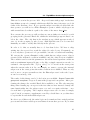
1. Preface
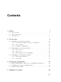
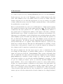
Figure 1.1: A simple process with examples of operators for loading, preprocessing and model production
via which they can communicate with the other operators in order to receive
input data or pass the changed data and generated models over to the operators
that follow. Thus a data flow is created through the entire analysis process, as
can be seen by way of example in fig. 1.1. Alongside data tables and models,
there are numerous application-specific objects which can flow through the process. In the text analysis, whole documents are passed on, time series can be
led through special transformation operators or preprocessing models are simply
passed on to a storage operator (like a normalisation) in order to reproduce the
same transformation on other data later on.
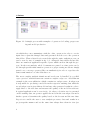
The most complex analysis situations and needs can be handled by so-called
super-operators, which in turn can contain a complete subprocess. A well-known
example is the cross-validation, which contains two subprocesses. A subprocess
is responsible for producing a model from the respective training data while the
second subprocess is given this model and any other generated results in order to
apply these to the test data and measure the quality of the model in each case.
A typical application can be seen in fig. 1.2, where a decision tree is generated
on the training data, an operator applies the model in the test subprocess and a
further operator determines the quality based on the forecast and the true class.
Repositories enable the user to save analysis processes, data and results in a
project-specific manner and at the same time always have them in view (see
2
1.1. The program
Figure 1.2: The internal subprocesses of a cross-validation
fig. 1.3). Thus a process that has already been created can be quickly reused
for a similar problem, a model generated once can be loaded and applied or
the obtained analysis results can simply be glanced at so as to find the method
that promises the most success. The results can be dragged and dropped onto
processes, where they are loaded again by special operators and provided to the
process.
In addition to the local repositories, which are stored in the file system of the
computer, RapidAnalytics instances can also be used as a repository. Since the
RapidAnalytics server has an extensive user rights management, processes and
results can be shared or access for persons or groups of persons limited.
The repositories provided by RapidAnalytics make a further function available,
which makes executing analyses much easier. The user can not only save the
processes there, but also have them executed by the RapidAnalytics instance
with the usual comfort. This means the analysis is completely implemented in
the background and the user can find out about the analysis process via a status display. The user can continue working at the same time in the foreground,
without his computer being slowed down by CPU and memory-intensive computations. All computations now take place on the server in the background, which
is possibly much more efficient, as can be seen in fig. 1.4. This also means the
hardware resources can be used more efficiently, since only a potent server used
jointly by all analysts is needed to perform memory-intensive computations.
3
1. Preface
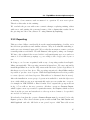
Figure 1.3: A well-filled repository
Figure 1.4: A process which was started several times on a RapidAnalytics instance. Some cycles are already complete and have produced results.
4
1.2. The environment
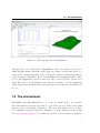
Figure 1.5: The R perspective in RapidMiner
Alongside the core components of RapidMiner, there are numerous extensions
which upgrade further functions, such as the processing of texts, time series or a
connection to statistics package R [1] or Weka [2]. All these extensions make use
of the extensive possibilities offered by RapidMiner and supplement these: They
do not just supplement operators and new data objects, but also provide new
views that can be freely integrated into the user interface, or even supplement
entire perspectives in which they can bundle their views like the R extension in
fig. 1.5.
1.2 The environment
RapidMiner and RapidAnalytics do of course not stand alone. No software
can exist without its developers and no open source project will be successful
without a live and kicking community. The most important point of contact
for community members and those wishing to become members is the forum
at http://forum.rapid-i.com, which is provided and moderated by Rapid-I.
5
1. Preface
Beginners, advanced users and developers wishing to integrate RapidMiner into
their own open source projects or make their own extensions available will all get
answers to their questions here. Everyone is warmly invited to participate in this
international exchange.
For all those wishing to get involved in a particular subject area, make their
own code available, or publish their own extensions, it is worthwhile becoming
a member of one of the Special Interest groups, which each concentrate on a
topic such as text analysis, information extraction or time series analysis. Since
Rapid-I developers also participate in this exchange, topics discussed here have
a direct influence in further development planning. Whoever would like to make
his own extension accessible to a larger public can use the necessary platform for
this - the Marketplace (see section 3.1). Here, users can offer their extensions and
choose from the extensions offered by other users. RapidMiner will, if desired,
automatically install the selected extensions at the time of the next start.
As a supplement to this, Rapid-I naturally offers professional services in the
RapidMiner and RapidAnalytics environment. As well as support for RapidMiner
and RapidAnalytics, training courses, consultation and individual development
relating to the topic of data analysis are offered.
1.3 Terminology
Before we begin with the technical part, it would be helpful to clarify some terms
first. RapidMiner uses terminology from the area of machine learning. A typical
goal of the latter is, based on a series of observations for which a certain target
value is known, to make forecasts for observations where this target value is not
known. We refer to each observation as an example. Each example has several
attributes, usually numerical values or categorical values such as age or sex. One
of these attributes is the target value which our analysis relates to. This attribute
is often called a label. All examples together form an example set. If you write
all examples with their attributes one below the other, you will get nothing other
than a table. We could therefore say table“ instead of example set“, row“
”
”
”
instead of example“ and column“ instead of attribute”“. It is helpful however
”
”
”
6
1.3. Terminology
to know the terms specified above in order to understand the operator names
used in RapidMiner.
7
2 The use cases
Having read the first section, you may already have one or two ideas why using
RapidMiner could be worthwhile for you. The possibilities offered by RapidMiner
in different use cases shall now be gone into in more detail. Two possible applications in the academic environment shall be presented at this stage: The first
relates in particular to researchers wishing to evaluate data mining procedures.
In section 2.1 we will show how this can be done in RapidMiner with existing
algorithms. After that we will show in section 2.2 how self-developed algorithms
can be integrated into RapidMiner and thus be used as part of this analysis.
Of course, data mining does not just serve as a purpose in itself, but can also be
applied. In section 2.3 we will show how data from application disciplines can be
analysed with RapidMiner.
All processes mentioned here are located in an example repository, which is available for download at http://rapid-i.com/downloads/documentation/academia/
repository_en.zip. In order to use it, the ZIP file must be extracted and the
directory created thereby must be added to RapidMiner as a local repository. To
do this, click on the first button in the toolbar of the Repositories view and select
new local repository“. Then indicate the name of the directory. You will now
”
find all example processes in the repository tree, which is shown in this view.
When reading this chapter it is recommended to open the processes contained
in this repository in RapidMiner so as to understand how they work. RapidMiner can be downloaded at http://www.rapidminer.com. The RapidMiner
user manual [3] is also recommended for getting started.
9
2. The use cases
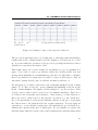
2.1 Evaluation of learning procedures
A typical and recurring task in the area of machine learning is comparing two or
more learning procedures with one another. This can be done to investigate the
improvements that can be obtained by new procedures, and also simply be used
to select a suitable procedure for a use case. In this section we will show how
this can be done with RapidMiner.
2.1.1 Performance evaluation and cross-validation
The numerous operators that apply machine learning procedures to datasets can
be easily used in combination with other operators. Typical examples of operators used in the evaluation of learning procedures are cross-validation, operators
for computing standard quality measures, parameter optimisations and last but
not least logging operators for creating procedure performance profiles. Since
RapidMiner supports loops, processes can also be created that apply the new
procedure to several datasets and compare it with other procedures. A process
that enables such a validation of one’s own procedure can be found in the example
repository.
If you look at the process 00.1 - Loop Datasets, you will see that it primarily
consists of three blocks: In the first block, some operators load a selection of
datasets, which are then combined with the Collect operator to form a Collection.
Of course, any of your own datasets can be loaded here.
In the second block, the datasets are iterated over: For this purpose, the internal
process is executed by the Loop Collection operator for each individual dataset
of the Collection. The dataset is copied directly in the subprocess of the loop
and led to three cross-validations. In each cross-validation there is a different
learning procedure. In this way the performance of all three learning procedures
is compared.
Within the loop, a Log operator records the respective results of the procedures.
In the third block, this log is converted into a dataset where all results are sum-
10
2.1. Evaluation of learning procedures
marized. It can now be saved, exported and viewed like every other dataset.
The second process 00.2 - Loop Files works in a very similar way. Instead of
loading the datasets from the repository individually, they are automatically
loaded from a collection of CSV files here. If there are several datasets available,
they can be easily and automatically used for testing in this way. The rest of the
process can remain unchanged here. Of course, other tasks can also be completed
in this way, such as transferring datasets into the repository.
2.1.2 Preprocessing
In many cases, procedures need preprocessing steps first in order to be able to
deal with the data in the first place. If we want to use the operator k-NN for the
k-nearest-neighbour method, we must note for example that scale differences in
the individual attributes can render one attribute more important than all others
and make the neighbourhood relation dominate in the Euclidean space. We must
therefore normalise the data in this case by adding a Normalize operator first.
However, if we add the Normalize operator before the cross-validation, all data will
be used to determine the average value and the standard deviation. This means
however that knowledge about the test part is already implicitly contained in
the training part of the normalised dataset within the cross-validation. Possible
outliers, which are only present in the test part of the dataset, have already
affected the scaling, which is why the attributes are weighted differently. This is
a frequent error which leads to statistically invalid quality estimations.
In order to prevent this, we must drag all preprocessing steps into the crossvalidation and execute them in the training subprocess. If we do not execute
any further adjustment in the process, the model generated in the training process will of course be confronted with the not yet normalised data in the test
process. This is why all preprocessing operators, the results of which depend
on the processed data, offer so-called preprocessing models. These can be used
to execute an identical transformation again. Thus the same average values and
standard deviations are used to transform at the time of normalisation, instead
of recomputing these on the current data.
11
2. The use cases
In order for these models to be used they just need to be transferred from the
training process to the test subprocess of the cross-validation. They can be
applied there with a usual Apply Model operator (like in the process 00.3 - Include
Preprocessing in Validation) before the actual model is applied.
2.1.3 Parameter optimisation
It is therefore very easy on the whole to perform a real validation of a procedure
in RapidMiner. However, almost every procedure has certain parameters with
which the quality of the models can be influenced. The results will be better or
worse depending on the setting. So if it is to be shown that a new procedure is
superior to an existing one, you cannot just optimise the parameters of your own
procedure or even set the parameters arbitrarily. The performance of procedures
such as the support vector machine or a neural network in particular depends
greatly on the parameter settings.
Therefore RapidMiner offers the possibility of looking for the best parameter
settings automatically. To do this, you use one of the Optimize Parameters operators. The operator Optimize Parameters (Grid) can be controlled most simply.
It iterates over a number (previously defined by the user) of combinations of the
parameters to be optimised. For each parameter combination it executes its internal subprocess. Accordingly, only parameters of operators of this subprocess
can be optimised. The subprocess must return a performance vector here (e.g.
the Accuracy), using which Optimize Parameters can recognise the quality of the
current combination. After it has tested all parameter combinations, the Optimize Parameters operator returns the combinations with maximum performance
measured in their cycle.
If not only the result as to the best combination is of interest, but also the general
progression for example, then it is worth using a Log operator. If the latter is
executed, it writes a new row into its log, which contains all values indicated by
the user. These values can either be the current values of any parameters of any
operators in the process or special values that vary from operator to operator.
All operators indicate for example the frequency with which they have already
12
2.1. Evaluation of learning procedures
been executed, the execution time and the like. Moreover, some operators give
additional information. For example, the cross-validation supplies the quality and
its standard deviation obtained at the time of the last execution. An example
which performs such an optimisation and logs all combinations in doing so can
be found in the process 00.4 - Optimize Parameters.
A further application for the Log operator can be found in the process 00.5 Create Learning Curve. This investigates how a learning procedure behaves in the
case of different training dataset sizes. For this purpose, a random sample of a
certain size of the entire dataset is made with a Sample operator. The quality of
the procedure can now be determined on this sample using the cross-validation.
Since this means that the quality depends greatly on the drawn sample, we have
to perform this several times in order to compensate for coincidental deviations
in a random sample. The smaller the original dataset, the more repetitions are
necessary. The Loop operator can be used to execute part of a process several
times. With the parameter iterations, it offers the possibility of indicating how
frequently its subprocess is to be executed.
This entire procedure must of course be performed for all different sample sizes.
We use the Loop Parameters operator for this, which helps us to configure the
parameter combinations with which its subprocess is to be executed. In this
case, we gradually vary the sample ratio parameter of the Sample operator in the
subprocess between and one hundred percent. We therefore get a very fine curve.
If the investigation takes too long, the number of steps can be reduced meaning
the subprocess does not need to be executed as frequently.
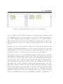
Within the subprocess of the Loop operator, we now just need to measure the
current sample ratio in each case and the accuracy obtained. Since we get several
results for each sample ratio however, we still need to introduce a postprocessing
step in order to determine the average and the standard deviation of the quality
over the different samples. For this purpose, the log is transformed into an example set in this process with the operator Log to Data, meaning we can aggregate
via the sample sizes and determine the average and the standard deviation. Thus
a dataset results from which we can read the quality as a function of the size of
the training dataset. In order to visualise the latter for a publication, we can use
13
2. The use cases
Figure 2.1: A diagram visualising the quality of the results
the Advanced Charts view. A possible result could then be as shown in fig. 2.1.
If we do not only wish to examine the binary decision of a model, but also how
the confidences are distributed, it is worth taking a look at the ROC plot, which
visually represents the so-called Receiver Operator Characteristic. The rule here
is that curves running further up on the left are better than curves further down.
The perfect classifier would produce a curve that runs vertically upwards from
the origin up to the 1 and horizontally to the right from there.
In RapidMiner, such a curve can be produced very simply and can also be compared very easily with other procedures. The test dataset just needs to be loaded
and placed at the input port of a Compare ROCs operator. All learning procedures
to be tested can subsequently be inserted into the subprocess. The results of the
procedures are represented together in a plot, as shown in fig. 2.2. The semitransparent areas indicate the standard deviation that results over the different
14
2.1. Evaluation of learning procedures
Figure 2.2: An ROC chart for comparing three models
cycles of the internally used cross-validation. An example of the comparison of
Naive Bayes, Decision Tree and a Rule Set can be found in the process 00.6 Comparing ROCs.
Last but not least, it should be noted that all plots and results can depend
on coincidental fluctuations. You should therefore not rely on a comparison of
the control criteria alone, but also test whether differences are significant. In
RapidMiner, the results of several cross-validations can be easily placed for this
purpose on a T-Test or Anova operator. You then get a table indicating the
respective test results. The level of significance can be indicated as a parameter
in doing so. A process that performs these tests on several datasets by way of
example can be found in 00.7 - Significance Test.
15
2. The use cases
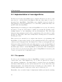
2.2 Implementation of new algorithms
We have now seen how algorithms can be compared. However, in order to evaluate new (i.e. self-developed) algorithms in this way, these must of course be
integrated into RapidMiner. RapidMiner was originally developed exactly for
this application: New algorithms were to be comfortably, quickly and easily comparable with other algorithms.
Implementing new learning procedures in RapidMiner is very easy. It is merely
necessary to create two Java classes, of which one performs the learning on the
training dataset, i.e. the estimating of the model parameters. The other class
must save these parameters and be able to apply the model to new data i.e. make
predictions. This will be introduced briefly in the following based on a fictitious
learning procedure.
This section is not intended as a complete introduction to programming with
RapidMiner. It just touches briefly on some principles and show how easily new
operators can be integrated into the framework, so that you can apply the evaluation procedures described in the preceding section to your own algorithms. A
complete documentation for developers of RapidMiner extensions can be found in
the white paper How to extend RapidMiner“ [6] and in the API documentation
”
[4]. If you are not a developer but want to discover RapidMiner from a user point
of view, you can feel free to skip this section.
2.2.1 The operator
In order to use a learning procedure in RapidMiner, it must be provided by an
operator like every other analysis step. To do this, we just need to create a
new subclass of Operator. For many kinds of operators there are specialised
subclasses which already provide various functions. In our case this is the class
AbstractLearner, from which all monitored learning procedures inherit. An
example implementation of such a procedure can be seen in fig. 2.3.
Essentially, only one method must be implemented which performs the training
16
2.2. Implementation of new algorithms
1
public c l a s s MyLearner extends A b s t r a c t L e a r n e r {
2
public s t a t i c void S t r i n g PARAMETER ALPHA = ” a l p h a ” ;
3
4
/* * Constructor called via reflection . */
public MyLearner ( O p e r a t o r D e s c r i p t i o n d e s c r i p t i o n ) {
super ( d e s c r i p t i o n ) ;
}
5
6
7
8
9
/* * Main method generating the prediction model . */
@Override
public Model l e a r n ( ExampleSet data ) throws O p e r a t o r E x c e p t i o n {
// Obtain user - specified parameter
i n t a l p h a = g e t P a r a m e t e r A s I n t (PARAMETER ALPHA) ;
MyPredictionModel model ;
// use data to create prediction model here
return model ;
}
10
11
12
13
14
15
16
17
18
19
/* * Define user - configurable parameters here . */
@Override
public L i s t <ParameterType> getParameterTypes ( ) {
L i s t <ParameterType> parameterTypes = super . getParameterTypes ( ) ;
parameterTypes . add (new ParameterTypeInt ( ” a l p h a ” ,
”The p a r a m e t e r a l p h a ” , 0 , 1 0 0 , 1 0 ) ) ;
return parameterTypes ;
}
20
21
22
23
24
25
26
27
28
/* * Tell the user what kind of input the algorithm supports . */
@Override
public boolean s u p p o r t s C a p a b i l i t y ( O p e r a t o r C a p a b i l i t y c a p a b i l i t y ) {
switch ( c a p a b i l i t y ) {
case NUMERICAL ATTRIBUTES :
case BINOMINAL LABEL :
return true ;
}
return f a l s e ;
}
29
30
31
32
33
34
35
36
37
38
39
}
Figure 2.3: Example implementation of a learning procedure in RapidMiner
17
2. The use cases
and then returns a model with the estimated model parameters, learn(). As an
input, it receives a data table in the form of an ExampleSet.
A learning procedure will usually offer different options to the user in order to
configure its behaviour. In the case of a k-nearest-neighbour method, the number of neighbours k would be such an option. These are called parameters in
RapidMiner and should not be confused with the model parameters (e.g. the
coefficient matrix of a linear regression). Each operator can specify these parameters by overwriting the method getParameterTypes(). In doing so, the range
of values (number from a certain interval, character string, selection from a set
of possible values, etc.) can be specified. The RapidMiner user interface then
automatically makes suitable input fields available for the configuration of the
operator. The parameter values selected by the user can then be queried and
used in the method learn() for example. In our example, the operator defines
a parameter with the name alpha.
The RapidMiner API offers numerous ways of supporting the user in the process
design, e.g. through early and helpful error messages. You can for example specify, by overwriting the method supportsCapability(),which data the learning
procedure can deal with. If there is unsuitable data, an appropriate error message will be supplied automatically and relevant suggestions made for solving this.
This can take place as early as at the time of process design and does not require
the process to be performed on a trial basis. In our example, the algorithm can
only deal with a two-class problem and numerical influencing variables.
2.2.2 The model
You now just need to implement the model which saves the estimated model
parameters and uses these to enable forecasts to be made with the model. In
the class hierarchy, the new class must be arranged below Model. For a forecast
model, it is worthwhile extending either PredictionModel or SimplePredictionModel
which make a simplified interface available. Such a class is outlined in fig. 2.4.
Essentially, the method learn() must be implemented, by iterating over the
ExampleSet and generating a forecast attribute by means of the estimated model
18
2.2. Implementation of new algorithms
1
public c l a s s MyPredictionModel extends P r e d i c t i o n M o d e l {
2
private i n t a l p h a ;
private double [ ] e s t i m a t e d M o d e l P a r a m e t e r s ;
3
4
5
protected MyFancyPredictionModel ( ExampleSet t r a i n i n g E x a m p l e S e t ,
i n t alpha ,
double [ ] e s t i m a t e d M o d e l P a r a m e t e r s ) {
super ( t r a i n i n g E x a m p l e S e t ) ;
this . alpha = alpha ;
this . estimatedModelParameters = estimatedModelParameters ;
}
6
7
8
9
10
11
12
13
@Override
public ExampleSet p e r f o r m P r e d i c t i o n ( ExampleSet exampleSet ,
A t t r i b u t e p r e d i c t e d L a b e l ) throws O p e r a t o r E x c e p t i o n {
// iterate over examples and perform prediction
return ex ampl eSe t ;
}
14
15
16
17
18
19
}
Figure 2.4: An example implementation of a forecast model
parameters. In our learn() method we could instantiate and return such a
model.
Exceeding the application for the purpose of a forecast, many models offer the
possibility of gaining an insight that can be interpreted by the user. For this
purpose, the model should be visualised in an appropriate way, which can be done
via a renderer. Details on this can be found in the API documentation [4] of
the class RendererService and in the white paper How to extend RapidMiner“
”
[6].
2.2.3 The integration into RapidMiner
In order to make the operator available in RapidMiner, the classes must be incorporated into an extension. For this purpose, the implemented operators are
19
2. The use cases
listed in an XML configuration file, meaning they can be mounted by RapidMiner in the right place within the operator tree. There is a template project
for this purpose, which can be imported into Eclipse for example and contains
an appropriate Ant script for building the extension. It also provides numerous
possibilities for comfortably creating documentation and other elements. You
simply copy the produced Jar file into the plugins directory of RapidMiner, and
then your extension is available. This too is detailed in the white paper How to
”
extend RapidMiner“ [6].
2.3 RapidMiner for descriptive analysis
Although the main application of RapidMiner lies in the area of inferential statistics, the numerous preprocessing possibilities can also be very useful in descriptive
statistics. The approach of the process metaphor offers quite different possibilities
for working on more complex data structures than is the case with conventional
statistics solutions. If regularly collected data is concerned for example, then the
processing can be automated as far as possible without any analysis efforts.
If you are not put off from drawing up scripts, the R extension of RapidMiner
provides access to all statistical functions offered by the world’s most widely used
statistics tool. These can also be integrated directly into the process in order to
fully automate the complete processing.
In the following we will look at a dataset containing information from a questionnaire. The questions were asked at various schools of different types as well
as at a university. We can use information concerning the sex and age of those
asked, otherwise the data remains anonymous. All information was entered into
an Excel table and we have already saved this data as 01 - Questionare Results
in the repository via the File menu and the item Import Data. Each question
of the questionnaire had a different number of possible answers, whereby only
one answer could be marked in each case. In order to save time during manual
inputting, the answers were consecutively numbered and only the number of the
marked answer was indicated in the table. A 0 designates a wrong or missing
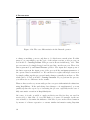
answer. Fig. 2.5 shows an excerpt from the table.
20
2.3. RapidMiner for descriptive analysis
Figure 2.5: An excerpt of the example data
21
2. The use cases
2.3.1 Data transformations
In a first analysis, we just want to obtain a rough overview of the general response
behaviour to start with. We would like to look at all groups together first all,
i.e. without any classification by sex or age. Our goal is to produce a table in
which each row represents a question and each column an answer. The relative
frequencies of the answers to the respective questions are to be indicated in the
cells of the tables.
Since we do not want to group at first, we remove all columns apart from those
containing the answers. To do this, we use the operator Select Attributes, as
demonstrated in the process 01.1.1 - Count Answers.
During importing we defined the columns as a numerical data type. Although
numbers are concerned, these do not represent a numerical value in the sense
that intervals can be determined or general arithmetic operations carried out
with them. We therefore want to transform the data type of the column into
a categorical type first. Attributes that can have different categorical types are
called polynominal in RapidMiner. Therefore the Numerical to Polynominal is
used.
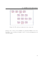
In order to obtain a column specific to each answer, we can now transfer the
polynominal column into a so-called Dummy Encoding. This standard technology,
which is frequently used when wishing to represent nominal values numerically,
introduces, for each nominal value, a new column which can take the value zero
or one. A one indicates that the original column contained the nominal value
represented by the new column. Accordingly, there is always exactly a one in
each row within the columns created in this way, as can be easily seen from the
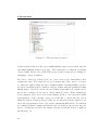
result of the transformation in fig. 2.6.
If we are interested in the average answer frequencies, we must now calculate the
average over all questionnaires submitted, for which it is sufficient to apply the
Aggregate operator with the preset aggregation function average. Since we want
to calculate the average over all rows, we do not select an attribute for grouping.
Thus all rows now fall into one group. We get a table as a result with one row per
group, so in this case with just one row indicating the relative answer frequency.
22
2.3. RapidMiner for descriptive analysis
(a) Before
the
transformation
(b) (B) After the transformation
Figure 2.6: Dummy coding of the response behaviour
The process is interrupted here by breakpoints, so that important intermediate
results such as the original dataset and the dummy-coded data can be looked
at. You can resume the execution of the process by pressing the Execute button
(which is now green) in the main toolbar.
This result cannot yet be used, neither for the human eye, nor for printing in a
paper. You could of course copy all these values into an Excel table now and
arrange them manually in a meaningful way, but since we still want to calculate
these very numbers for subgroups, it would be better at this stage to find an
automated variant directly, since it will save us much work later on.
For this purpose, we want to first remove the redundant average from the column
names. To do this, we use the operator Rename by Replacing, as shown in the
01.1.2 - Count Answers. We simply add the changes to our process here. This
operator uses so-called regular expressions for renaming attributes. These are a
tool that is also frequently used elsewhere. Since many good introductions to
this topic can be easily found on the internet, we will not go into detail here.
For your experiments you can use the assistant, which you can get to by pressing
the button next to the input field for the regular expression. You can apply an
expression to a test character string here and immediately get feedback as to
whether the expression fits and on which part. In our example, we replace the
attribute name with the content of the round brackets in the attribute name using
23
2. The use cases
a so-called Capturing Group. Average (Question1) therefore becomes Question1.
In the next step, we come to the Transpose operator, which transposes the data
table. All columns become rows, whilst each row becomes a column. Since the
dataset only had one row after the aggregation, we now get exactly one regular
column, whilst the newly created id column contains the name of the attributes
from which the row was formed.
Based on the id attribute we can now see which answer to which question spawns
the calculated frequency value in the regular attribute att 1. The values in the id
column have the form question X = Y“, whereby X designates the number of
”
the question and Y designates the number of the answer. We want to structure
this information more clearly by saving it in two additional new attributes. For
this purpose we will simply copy the id attribute twice and then change the values
with a Replace operator in such a way that they clearly identify the question on
the one hand and the answer on the other. The Replace operator in turn uses
regular expressions. We will also use the Capturing Group mechanism here to
specify which value is to be applied. The result after these two operators looks
much more readable already, although it is still unsuitable for printing. A wide
format where each question occupies one row and the answers are arranged in
the columns would be much more practical and compact.
We will now launch into the last major step in order to transform the data
accordingly. For this purpose, we attach a Pivot operator to our current process
chain, as in the process 01.1.3 - Count Answers. This operator will ensure that
all rows which have the same value in the attribute designated by the parameter
group attribute are combined to make a single row. Since we want to describe
each question with a row, we select the attribute Question for grouping. So that
we get one column per answer option, we select the attribute Answer as the
index attribute. Now a new column will be created for each possible answer.
If there is a question/answer combination in the dataset, the appropriate cell
will be indicated in the row of the question and the column of the answer. If
there is no combination, this is indicated by a missing value. This can be easily
observed in the result, since there is only one question (i.e. question 1) with five
answer options - all other values in the relevant column are accordingly indicated
24
2.3. RapidMiner for descriptive analysis
as missing. Some answers, such as answer 1 to question 17, were never given.
Therefore this value is also missing.
We conclude the process with some cosmetic changes, replacing missing values
with a zero and putting the generated names of the columns that resulted from
the pivoting into the form answer X“ using Rename by Replacing.
”
2.3.2 Reporting
This procedure differs considerably from the usual manipulating of tables, as is
known from spreadsheets and similar software. Why is worthwhile switching to
such a process-orientated approach? We see why the moment we want to perform
recurring tasks several times. We will illustrate this again by using our example.
We have only evaluated the created table for all participants up to now and now
want to look at different groupings, e.g. according to school type, school year or
sex.
In doing so, we become acquainted with a way of exporting results from RapidMiner automatically. The reporting extension helps us here. We can comfortably
install RapidMiner now via the Help menu with the item Update RapidMiner if
this has not yet been done (note: The reporting extension for RapidMiner makes
it possible to produce static reports. With the RapidAnalytics server it is possible
to create dynamic web-based reports. This will not be discussed here however.)
After the installation, a new group of operators is available to us in the Operators
view, with which we can now automatically write process results into a report,
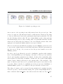
for example in PDF, HTML or Excel format. If we expand the group as shown
in fig. 2.7 we will see six new operators. Of these operators, Generate Report,
which begins a new report under a particular name, and Report, which receives
data from the process and attaches it to the report in a format to be specified,
are needed for each report.
It is already clear that the operator Generate Report must be executed before the
Report operator. The other relevant operators such as Add Text, Add Section and
Add Pagebreak each also fall back on an opened report. Add Text adds a text
25
2. The use cases
Figure 2.7: The reporting operators
at the current position of the report, Add Section begins a new breakdown level
and Add Pagebreak starts a new page. The result may be different depending
on the format. In the case of Excel files, page breaks correspond for example to
changing to a new worksheet.
In order to draw up a first report, we open a new report immediately after
loading the data. Note that the report is written into a file, and so you have
to adapt the path if using the 01.2 - Report Counts. An Add Section operator
produces a new Excel sheet, which we can give a name with the parameter report
section name. We then execute the processing steps until now, which can be
moved into a subprocess in order to divide them up better. If the results have
been computed, all you now need is the Report operator. You can select which
representation of the relevant object you would like to insert into the report
using the button Configure Report. Since we are interested in the data here, we
select the representation Data View under paramvalueData Table. It can then
be configured which columns and which rows one wants to incorporate into the
report – in this case we select all of them. Our process should now be roughly as
shown in fig. 2.8.
26
2.3. RapidMiner for descriptive analysis
Figure 2.8: A simple reporting process
As we can see, the reporting is smoothly inserted into the process logic. But
we are of course not only interested in the overall response behaviour, but want
to discover differences between the participant subgroups in particular. We will
use the following trick for this: We use a Loop Values operator that performs
its internal subprocess for each occurring value of a particular attribute. In this
subprocess we will reduce the dataset to the rows with the current value, then
aggregate as it usual and finally attach it as a report element.
Since we are interested in different groupings, we use a Multiply operator in order
to process the original dataset several times and insert different representations
into the report. In fig. 2.9 you can see how the process branches out at the
Multiply operator.
In order to use loops effectively, we need to familiarise ourselves with a further
facet of the RapidMiner process language: the macros. These process variables
can be used anywhere parameters are defined. A macro has a particular value
and is replaced by this value at runtime. In this case, the operator Loop Values
defines a macro which is allocated to the current value of the attribute. The
macro is therefore used here as a loop variable and is given a new value in each
loop pass. Macros can also be explicitly set in the process via a Set Macro or
Generate Macro operator or be defined for the process in the Context view.
The value of a macro can be accessed in any parameters by putting its name
between %{ and }. In the standard setting, the operator Loop Values will set a
macro with the name loop value. One then accesses its value via %loop value.
27
2. The use cases
Figure 2.9: A reporting process
28
2.3. RapidMiner for descriptive analysis
This can be seen in the process “01.3 - Report Counts with groups” in the first
Loop Values operator for example, which was called Sex, since it iterates over both
forms of the attribute Sex“. If you open the subprocess with a double-click, the
”
first operator you will see is a Filter Examples operator, which only keeps rows
with an attribute Sex that is equal to the value of the macro loop value.
If we execute the process, we will see that an own worksheet is created for each
grouping in the generated Excel file, whilst the individual groups are listed one
below the other. The only flaw is the student group, which appears as school
year 0“ in the grouping by school year. Although this can soon be remedied
”
manually, we want to rectify this directly in the process.
In order to do this, we actually have to do less than before. We have to skip
writing into the report if we reach the value 0 for school year. Fortunately, we
do not only have operators for loops available, but also a conditional branching.
We can use the operator Branch for this, which has two subprocesses. One is
executed if the indicated condition is fulfilled, and the other if it is not fulfilled.
The condition can be set in the parameters. As well as data-dependent conditions
such as a minimum input table size or the like, a simple expression can also be
evaluated. An expression like ”%{loop value}”==”0” is true at the exact point
when the current value is 0. In our example, we want to execute the internal
subprocess at the exact point when this condition is not fulfilled. Thus we only
need to move our process until now into the Else subprocess for the school year,
as can be seen in fig. 2.10.
The result of this change can be looked at in process 01.04 - Report Counts with
groups and exceptions - Report Counts with groups and exceptions. After performing the change, the rectified Excel file is available to us. The only annoying
thing when drawing up our report is the fact that we have inserted exactly the
same functionality into the subprocesses over and over again each time - once
for each kind of grouping. The complete subprocesses can of course be simply
copied, but if you want to supplement or modify a detail later on you then have
to repeat this in each individual subprocess.
In order to avoid this work, the entire logic can be transferred into an independent
process and the latter called up several times from another process. If you want
29
2. The use cases
Figure 2.10: The case differentiation in the Branch operator
to change something, you now only have to do this from a central point. For this
purpose, we can simply copy the logic of the subprocess into a new process, as
seen in 0.1.5 - Counting Process. This process is shown in full in fig. 2.11. This
process can now be simply dragged and dropped into another process. There it is
then represented by an Execute Process operator. The input and output ports of
the latter represent the input ports of the process if the use inputs parameter of
the operator has been switched on. We can therefore replace all subprocesses now
by simply calling up this process and make changes centrally from then on. The
result can be looked at in 01.5 - Reusing Processes. If you perform the process,
you will notice no difference in the results.
Thus we have seen how you can easily produce a report with statistical evaluations
using RapidMiner. If the underlying data changes or is supplemented, you can
quickly update the report by re-executing the process, especially in the case of
fully automatic execution in RapidAnalytics.
Of course, it is also possible to apply prediction models (as they are used in
section 2.1) to this data. So it would make good sense for example, in the use
case at hand, to determine the influence of the school year on the selected answers
by means of a linear regression or extract similar information using Bayesian
30
2.3. RapidMiner for descriptive analysis
Figure 2.11: The entire processing logic as an own process
methods. As you can see, the possibilities are practically unlimited. If you try
RapidMiner out you will most certainly be able to develop and implement your
own ideas quickly.
31
3 Transparency of publications
In section 2.1 we used RapidMiner to perform as complete an evaluation of a new
procedure as possible with little effort. We saw how to establish the evaluation
on a wide data base, how to optimise parameters fairly for all procedures and
how to evaluate the results. If you are pleased with the results, you may now
want to publish your results in a magazine, at a conference or in a book. A
good publication should enable the reader to understand, compare and continue
developing the obtained results and perform further analyses based on these.
In order to ensure this, three components are necessary: The implemented new
algorithms, the performed processes and the used data. These can of course not
(or not sufficiently) be printed as part of a publication, but could be easily made
accessible by linking to internet sources.
Unfortunately, experience shows that this is often not the case. This leads to
a large part of scientific work being used to reproduce work already done for
comparison purposes instead of reusing results.
In this chapter we will show how, using suitable portals on the internet, algorithms, processes and data can be easily published and made accessible for the
academic world as well as possible users.
You will therefore increase the quality of your publication and the visibility and
quotability of your results significantly.
33
3. Transparency of publications
3.1 Rapid-I Marketplace: App Store for
RapidMiner-extensions
In order to make self-implemented procedures accessible to the public, it makes
good sense to offer them on the Marketplace for RapidMiner. You will find this
at http://marketplace.rapid-i.com. On this platform, every developer can
offer his RapidMiner extensions and use extensions provided by other developers.
Using the marketplace is free of charge for RapidMiner users and for extension
providers. Extensions offered on the Marketplace can be installed and updated
directly from the RapidMiner user interface. The function Update RapidMiner is
available in the Help menu for this purpose. This is therefore the simplest kind
of installation for the user.
The Marketplace offers a number of advantages compared to publication on internal institute pages: This includes optimum visibility in the RapidMinerCommunity, simple installation and commenting and rating functions. If a user opens a
process which needs your extension, but the user has not installed it, RapidMiner
will automatically suggest the installation.
Even if you decide to make a publication on the Marketplace, there is no harm in
continuing to run your own page offering documentation, examples, background
information and possibly source code. This is even explicitly recommended, and
a link to this page can be created in the Marketplace.
In order to offer an extension, just register at http://marketplace.rapid-i.com
and then send a hosting query via the contact menu. This will be briefly examined
by Rapid-I for plausibility and conflicts with other extensions and will then be
confirmed within the shortest time.
Please note that it is of course all the more important to adhere to the general
naming conventions, spelling and documentation guidelines if you want to make
the extension accessible to other users. This should definitely be considered
from the beginning, since the changing of parameter names or operator keys for
example renders processes created up to that point unusable. The parameters
for other users should also be given as self-explanatory a name as possible and
34
3.1. Rapid-I Marketplace: App Store for RapidMiner-extensions
Figure 3.1: The descriptions of RapidMiner extensions can be edited in the Marketplace (in this case the Community Extension, which is described
below).
35
3. Transparency of publications
be well-commented. A detailed documentation and example processes then put
the icing on the cake in terms of comfort.
3.2 Publishing processes on myExperiment
Irrespectively of whether you use a self-implemented RapidMiner extension in
your processes or not, it is often desirable to share your own processes easily with
the community of scientists and data analysts. The portal myExperiment.org is
a social network that addresses scientists and offers the possibility of exchanging
and discussing data analysis processes.
By making your RapidMiner processes available on this site, you will achieve a
greater distribution of your results and ensure a clear and lasting quotability at
the same time. You will continue to benefit from the opportunity to exchange
with other scientists and make new research contacts. Last but not least, myExperiment can be an outstanding source if you are looking for inspiration regarding
the solution of a data analysis problem – no doubt others have already dealt with
similar problems.
In order to use myExperiment, you do not have to painstakingly upload or download the processes via a web browser. Instead, you can do this directly from the
RapidMiner user interface using the Community Extension. You can also install
these via the Marketplace (and the RapidMiner update server). As soon as you
have done this, RapidMiner will have a new view named MyExperiment Browser.
You can activate this via the View menu and the item Show View. You can sort
this view into any place within any perspective and of course hide it again.
The browser allows you to log in with an existing user account or register with
MyExperiment in order to create a user account. You will need this account to
upload processes. All processes saved on MyExperiment are shown in the list. If
you select an item in the list, the picture of the appropriate process will appear
in the right-hand window as well as the description and meta data such as author
and date of creation. This process can then be simply downloaded with the Open
button and opened and executed directly in RapidMiner. Alternatively, you can
36
3.3. Making data available
Figure 3.2: The RapidMiner Community Extension for accessing myExperiment
also look at the process in the browser via the myExperiment website. To do
this, just click on the Browse button. A process can also be clearly identified
with the URL opened here, meaning it can be used for quoting.
In order to upload your own process on myExperiment, open the desired process
and arrange it in the desired way. The subprocess currently displayed is uploaded
as a picture on myExperiment and appears when browsing. So an attractive and
clear arrangement pays off here. You can then click on Upload in the Browse
MyExperiment view. The window shown in fig. 3.2 opens and offers you fields for
entering a title and a description. The general language used on myExperiment
is English.
3.3 Making data available
MyExperient cannot undertake the task of saving the data as there are not enough
resources, therefore the publishing of our data has to be done by other means,
37
3. Transparency of publications
provided that it is allowed to publish the data and there are no restriction as a
result of copyright or data confidentiality. Thanks to the capability of RapidMiner
to use data from nearly any source this is not a problem.
What would probably be the simplest way in many cases would be to export
the data first as a CSV file and store the exported file on any web server. In
RapidMiner, we can now open this address with an Open File operator which
can also process data from internet sources. This operator does not interpret the
data first of all, but supplies a File object for this file. We can then place this
object at the file entrance of the Read CSV operator in order to interpret the file
as a CSV and load the dataset. The Read CSV operator can be easily configured
with the wizard, and the wizard can be executed on a local copy of the file for the
sake of convenience. If you now remember to set the same encoding at the time
of export as a CSV and at the time of import, there will be no longer anything
standing in the way of publication.
If experiments are conducted on large datasets or datasets containing a lot of
text, the datasets can also be stored compressed in a Zip file and you can have
these extracted by RapidMiner. This avoids unnecessary waiting times when
downloading and a high server utilisation. Both cases are demonstrated in the
process 00.8 - Load Data from URL.
38
4 RapidMiner in teaching
Using RapidMiner is also worthwhile in teaching. This offers several advantages.
One of the biggest advantages is without doubt the fact that RapidMiner is
available for free download in the Community Edition. Students can therefore
install it on their private computers in just the same way as the university can
make RapidMiner installations available on institute computers. Thus getting
started is fast and free of charge. Thanks to RapidMiner’s wide distribution,
students also have the opportunity during their studies of working with a tool
that they may actually use at work later on.
The numerous learning procedures contained in the core and in the extensions
cover the majority of typical lectures in the areas of data mining, machine learning and inferential statistics. It is therefore possible for the student to use and
compare the learned procedures directly without too much effort, leading to a
longer learning effect than with a purely theoretical observation of the algorithms
and their characteristics.
It is not unusual for students to develop their own algorithms and learning procedures in the context of internships, seminars, assignments or exercises. If this
takes place within the RapidMiner framework, existing infrastructure can be
reused. Evaluating the procedure or connecting to data sources for example is
made substantially easier. In this way the students can concentrate on implementing the actual algorithm. Besides, it is highly motivating for the student if
the result of such work can continue to be used after they have graduated. In the
case of distribution as a RapidMiner extension, this is much more likely than with
39
4. RapidMiner in teaching
a single solution that is not incorporated in any framework. This is heightened
further by the increased visibility when using the Rapid-I Marketplace.
Since many universities already use RapidMiner in teaching, there is already a
wealth of experience as well as teaching materials that can be reused.
Joining the mailing list
https://lists.sourceforge.net/lists/listinfo/rapidminer-sig-teaching
is worthwhile for exchanging experiences, materials and ideas for teaching with
RapidMiner.
40
5 Research projects
Finally, we would now like to outline once more how RapidMiner is actually used
at Rapid-I for research purposes. This chapter gives an overview of the various
ways in which data mining techniques can be used in various disciplines and also
be a stimulus for future projects.
e-LICO. (http://www.e-lico.eu) Within this EU project, in which eight universities and research establishments were involved alongside Rapid-I, a platform
was developed from 2009 to 2012 enabling even expert scientists without a statistical or technical background to use data mining technologies. One of the things
created was an assistant which fully automatically generated data mining processes after the user had specified input data and an analysis goal with a few
clicks. The development of the server solution RapidAnalytics also began in the
context of this project.
ViSTA-TV. (http://vista-tv.eu/) This project, which was also funded by the
EU in the Seventh Framework Programme, is concerned with the analysis of data
streams as they are generated by IPTV and classic television broadcasters. The
goal is to improve the user experience by offering suitable recommendations for
example and an evaluation for market research purposes.
SustainHub. (http://www.sustainhub-research.eu/) Unlike the two projects
first mentioned, the SustainHub project is not rooted in an IT-oriented but in
an application-orientated EU funding programme. It concerns the utilisation of
41
5. Research projects
sustainability information in supply chains and the recognition of abnormalities
for the purpose of risk minimisation. Methods of statistical text analysis are also
used to automatically investigate messages for their relevance to this topic.
ProMondi. The goal of the ProMondi project funded by the Federal Ministry of
Education and Research (BMBF) is to optimise the product development process
in the manufacturing industry. For example, the influences on assembly time are
to be recognised by data mining techniques as early as at design time and suitable
alternatives determined.
Healthy Greenhouse. (http://www.gezondekas.eu) The project Gezonde
”
Kas“ is an Interreg IV A EU programme, within the framework of which ten
research establishments and 22 enterprises from the German-Dutch border area
are developing an innovative integrated plant protection system intended to enable a sustainable management of modern horticultural enterprises. Data mining
techniques are used here for example to recognise possible diseases and pests early
on and get by with fewer pesticides or to analyse the influence of environmental
factors on plant growth and health.
This overview may be a stimulus for your own research ideas. Rapid-I will continue to conduct both application-orientated projects and projects in the field
of data mining on a national and international level. If you are interested in a
research partnership, get in touch at [email protected].
42
Bibliography
[1] The R project for statistical computing. http://www.r-project.org/.
[2] Weka 3: Data mining software in Java. http://www.cs.waikato.ac.nz/ml/
weka/.
[3] Rapid-I GmbH. RapidMiner Benutzerhandbuch, 2010. http://rapid-i.
com/content/view/26/84/.
[4] Rapid-I GmbH. RapidMiner API documentation. http://rapid-i.com/
api/rapidminer-5.1/index.html, July 2012.
[5] Marius Helf and Nils Wöhler. RapidMiner: Advanced Charts, 2011. Rapid-I
GmbH.
[6] Sebastian Land.
How to extend RapidMiner 5.
http://rapid-i.
com/component/page,shop.product_details/flypage,flypage.tpl/
product_id,52/category_id,5/option,com_virtuemart/Itemid,180/,
2012. Rapid-I GmbH.
43