Download User Manual

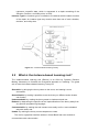
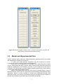
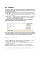
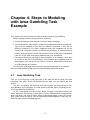
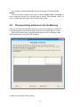
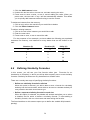
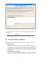
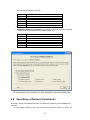
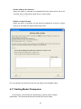
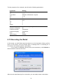
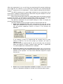
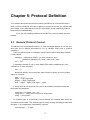
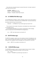
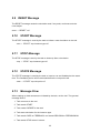
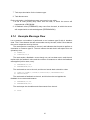
User Manual
for the Instance-based Learning Tool
Dynamic Decision Making Laboratory
Carnegie Mellon University
Version 1.3.40, September 7, 2010
Privileged and confidential: please do not quote or distribute without permission.
Copyright ©2009–2010 Dynamic Decision Making Laboratory. All rights reserved.
Do not distribute without express written permission from Dr. Cleotilde Gonzalez, Director
of the Dynamic Decision Making Laboratory at Carnegie Mellon University, Pittsburgh.
Please send requests for errata to the author.
1
Table of Contents
Chapter 1: Overview....................................................................................3
Chapter 2: Introduction...............................................................................4
2.1 What is the Instance-based Learning Theory? .................................4
2.2 What is the Instance-based Learning tool?.......................................5
Chapter 3: Getting Acquainted with the Tool ...........................................6
3.1 Installing............................................................................................6
3.2 User Interface ...................................................................................6
3.3 Model and Experimental Files...........................................................8
3.4 Formulas ...........................................................................................9
3.4.1
Formula Components ..............................................................9
3.4.2
Function Calls ........................................................................11
3.4.3
Debugging Formula Errors.....................................................14
3.4.4
Formula Limitations................................................................16
Chapter 4: Steps to Modeling with Iowa Gambling Task Example .......17
4.1
Iowa Gambling Task .....................................................................17
4.2
Defining Instance Types................................................................18
4.3
Pre-populating Instances into the Memory....................................19
4.4
Defining Similarity Formulas .........................................................20
4.5
Choosing a Retrieval Method........................................................21
4.6
Specifying a Retrieval Constraints ................................................23
4.7
Setting Judgment Heuristics .........................................................24
4.8
Defining Decision-Calculation Formulas .......................................25
4.9
Defining Feedback Formulas ........................................................27
4.10 Selecting a Utility Update Method .................................................28
4.11 Setting Model Parameters.............................................................29
4.12 Executing the Model......................................................................32
4.13 Previewing and Exporting Experimental Results ..........................33
Chapter 5: Protocol Definition..................................................................37
5.1
General Protocol Format...............................................................37
5.2
ALTERNATIVE Message ..............................................................38
5.3
BATCH Message ..........................................................................38
5.4 CUESIZE Message.........................................................................38
5.5 DECISION Message .......................................................................39
5.6 ERROR Message ...........................................................................39
5.7 FEEDBACK Message .....................................................................39
5.8 FEEDBACKOK Message................................................................39
5.9
RESET Message...........................................................................40
5.10 START Message...........................................................................40
5.11 STOP Message.............................................................................40
5.12 STATE Message...........................................................................40
5.13 Message Flow...............................................................................40
5.14 Example Message Flow................................................................41
Bibliography...............................................................................................42
2
Chapter 1: Overview
This report contains information on how to use the Instance-based Learning tool
(IBLtool). The document is written to explain the IBLtool to beginners in modeling
techniques as well as to advanced users of modeling and instance-based learning.
Chapter 2 serves as a short introduction to the tool, the theory behind it, and the
goals of this tool.
Chapter 3 contains an overview of the tool and its interface.
Chapter 4 takes the Modeler through the steps necessary to create a working
model from the beginning to end.
Chapter 5 describes the protocol necessary to connect a task to the tool.
3
Chapter 2: Introduction
2.1
What is the Instance-based Learning Theory?
The Instance-based Learning Theory (IBLT) was initially proposed to demonstrate
how learning occurs in dynamic decision-making tasks (Gonzalez et al., 2003). An
IBLT model was implemented within the ACT-R architecture (Anderson and
Lebiere, 1998), and we demonstrated how IBLT parameters were needed to
account for human decision making in a dynamic and complex task. IBLT has more
recently been used in other tasks in addition to dynamic decision making. These
include simple binary choice tasks and two-person game-theory learning
(Gonzalez & Lebiere, 2005).
Under the IBLT, modelers determine the representation of declarative knowledge
(chunks or instances) in a task. In IBLT, an instance is a triple containing the cues
that define a situation (S), the actions that define a decision (D), and the expected
or experienced value resulting from an action in such situation (U). Simply put, an
instance is a concrete representation of the experience that a human acquires in
terms of the decision-making situation encountered by the human, the decision the
human makes, and the outcome (feedback) the human obtains.
A modeler following the IBLT approach must define the structure of an SDU
instance. Then, an ACT-R modeler following the IBLT approach should define
productions that represent the generic decision-making and problem-solving
process proposed by IBLT. This process involves the following steps:
• Recognition, the comparison of cues from the environment or task to cues
from memory;
• Judgment, the calculation of the possible utility of a decision in a situation,
either from past memory of from heuristics;
• Choice, the selection of the instance containing the highest utility; and
• Feedback, the modification of the expected utility defined in the judgment
process with the experienced utility after receiving the outcome from a
decision made.
The IBLT mechanisms involve a set of functions and thresholds, including a
similarity function used in the recognition step to determine what instances from
memory are similar to the current situation; the decision threshold used in the
choice step to determine whether more “evidence” or alternative search is needed
before a selection is made; and the feedback threshold used to determine “how
much” of the outcome provided from the environment is accounted for in the utility
of the instances.
Instance An instance is the smallest unit of an experience. It is a set of values that
4
represent a specific state, which is expressed in a triplet consisting of the
Situation, Decision, and Utility slots, or SDU.
Instance Type An instance type is a collection of instances with the same structure
of the triplet. An instance type may contain more than one of each: situation,
decision, and utility slots.
Figure 2.1: Instance-based Learning Theory
2.2
What is the Instance-based Learning tool?
The Instance-based Learning tool (IBLtool) is an effort by Dynamic Decision
Making Laboratory to formalize the theoretical approach to modeling. The goals
are to have the Instance-based Learning Theory be:
Shareable: by bringing the theory closer to the users, and making it more
accessible;
Generalizable: by making it possible to use the theory on different and a diverse
set of tasks;
Understandable: by making the theory easier to implement and use;
Robust: by abstracting the specifics of the implementation of the theory away from
any specific programming language;
Communicable: by making the tool interact more easily and in a more standard
way with tasks; and
Usable: by making the theory more transparent to users.
The tool is a graphical interface written in Visual Basic that uses sockets to
communicate with various tasks.
5
Chapter 3: Getting Acquainted
with the Tool
In this chapter, we will get acquainted with the user interface of the IBLtool, and get
started with the basic concepts that will help you as you move through the
modeling process.
3.1
Installing
To use the IBLtool on your computer, you will need a few things:
1. a Windows XP, Windows Vista, or Windows 7 machine, with the latest
software updates; and
2. the installer package for the tool. There are separate installer packages for
Windows XP and Windows Vista, so ensure you have the correct installer.
The Windows Vista installer also doubles as the Windows 7 installer.
To install the tool, unzip the installer package, and run the setup.exe file.
When upgrading the tool, it is recommended that you uninstall previous
versions of the software before installing the new version. It is also recommended
that you back up your model files before attempting an upgrade or uninstall, in
order to ensure that your work remains preserved.
To ensure that the installation succeeded, start IBLTool by going to the Start
Menu > DDMLAB > IBLTool. The tool comes with two sample model files: a
binary choice task, and the Iowa Gambling Task. We will use the latter in the next
chapter as an example on constructing a model from scratch.
3.2
User Interface
The tool is presented as a graphical user interface. It is arranged into successive
screens. One of the screens can be seen in Figure 3.1.
Each screen is divided into three areas:
Instructions Each screen shows a short set of instructions for actions pertinent to
the screen. Instructions appear at the top of the screen.
Content The bulk of a screen’s functionality, or content, appears in the middle of the
screen. Most screens have a tabbed interface, in which each tab in the tabbed
interface represents an instance type. The tabbed interface aims to separate
6
each instance type and reduce confusion as to which instance type is currently
being worked on.
Buttons At the bottom of every screen is a collection of buttons. The left-most and
right-most buttons are navigation buttons and can be used to move to the
previous and next screens, respectively.
Figure 3.1: An example of a screen in the tool.
In order to ease the process of jumping between non-consecutive screens, the tool
also presents you with a navigation window. The tool exits only when this
navigation window is closed. The navigation window also provides means to open
different models and save your entire model to a different file. (Figure 3.2)
7
Figure 3.2: iBLTool navigation window: when no model is opened (left), and when the
model saved in instances.mdb is opened (right).
3.3
Model and Experimental Files
All your instance types, instances, model parameters, and formulas for your model
are automatically saved into a model file.
To move your model between computers, copy the model file to another
computer. Be sure to install the tool on both computers.
When you run an experiment or simulation, your model file will be copied
into an experimental file with a similar name. Experimental files also include all
instances, parameters, and formulas you have in your model file at the time of
simulation. This allows you to modify models between experiments, without having
to save each model with a different name.
Model and experimental files can and may be opened using a copy of
Microsoft Access, which can be useful when post-processing data collected during
simulation. While it is also possible to modify tool parameters directly from
Microsoft Access, we strongly recommend doing so through the tool instead, to
prevent the possibility of corrupting any configuration parameters.
8
3.4
Formulas
Formulas and formula editors are large parts of the tool, because they allow users
to write their own formulas using simple arithmetical operations. Formula editors
are divided into three sections:
Formula Entry The Formula Entry box is where the user will enter their formula.
Variable List The Variable List box shows a list of variables available for use in
that formula. Clicking a variable in the Variable List will insert that variable in
the Formula Entry box.
Formula Status The Formula Status box shows whether there are any errors in
the formula, if the tool expects the formula to define a certain variable, or if
the formula was accepted without any errors.
One important point to note is that formulas written in the formula editor will be
automatically checked for errors, and automatically saved.
Figure 3.3: Formula Editor, consisting of Formula Entry (top left), Variable List (top right),
and Formula Status (bottom). In this example, the formula has been successfully accepted
by the tool, i.e. the formula has no errors and all the variables are correctly defined.
3.4.1 Formula Components
Formulas and all its contents—including variables—are case insensitive, i.e. abc is
equivalent to ABC. This case-insensitivity will prevent many errors.
Formula A formula consists of one or more Statements. Each Statement must
appear on its own line.
Statement A statement can be: (a) an Assignment, or (b) an IF Conditional.
Assignment An assignment is used to assign a value—or another variable— to a
variable. Variable names must start with a letter, but may be followed by any
alpha-numeric character (A-Z and 0-9) or a period. For example, these are valid
variable names: A, A6, MEMORY, MEMORY.GOAL.
Example formula:
A = 5
9
B = A
The formula above consists of two statements, both of which are
assignments. When the formula is run, as expected, both A and B will
carry the value 5.
Assignments are evaluated in order. Thus, the following formula:
A = 10
A = 12
will set the value of A to 12.
IF Conditional An IF conditional is used to perform different tasks depending
on a set of conditions.
There are two syntaxes for IF conditionals:
IF condition THEN
statement1
ENDIF
and:
IF condition THEN
statement1
ELSE
statement2
ENDIF
The first syntax allows a conditional statement to not do anything if the
condition is not met.
The condition above is an Expression. Both statement1 and
statement2 are regular statements, which would allow the user to have
complex rules and nested conditionals, e.g.:
IF condition THEN
statement1
ELSE
IF other-condition THEN
statement2
ENDIF
ENDIF
Expression An expression may be:
1. a variable or value, e.g. TIME or 5;
2. a function call, e.g. ABS(CUE.GOAL)(see section on Function Calls);
3. a mathematical computation, e.g. TIME + 5, which uses a
mathematical operator (see Table 3.1: Mathematical Operators);
4. a comparison, e.g. TIME + 5 > 10, which uses a comparison
operator (see Table 3.2: Comparison Operators); or
5. a logical expression, e.g. (TIME + 5 > 10) AND (GOAL < 6),
10
which uses a logical operator (see Logical Operators), and connects
other expressions together.
Operator
Description
Example
+
−
∗
/
\
Addition
Subtraction
Multiplication
Division
Division with rounding
down
5 + 2
CUE.GOAL - MEMORY.GOAL
A * B
A / B
A \ B
∗∗
Exponentiation
2 ** B
Table 3.1: Mathematical operators and their examples.
Operator
Description
Example
==
<> or ! =
>
>=
<
<=
Equality
Inequality
Greater than
Greater than or equal to
Less than
Less than or equal to
MEMORY.TIME == CUE.TIME
MEMORY.TIME <> CUE.TIME
A > -5
A >= -5
A + B < 2 * A
A + B <= 2 * A
Table 3.2: Comparison operators and their examples.
Function call A function call is used to invoke one of the predefined functions in
the tool; it uses the function call operator (), and takes arguments. Each
argument is separated by a comma, and an argument is simply any valid
expression. For example:
Q = ABS(NOISE)
calculates the absolute value of the variable NOISE and saves the result
into variable Q. The function name in this case is ABS, and it has one
argument, denoted by (NOISE).
3.4.2
Function Calls
The IBLtool has various function calls available for use. In this section, we will list
them all, and describe how to use them.
ABS(expr1) This function expects one argument and computes the absolute
value of that argument.
AVERAGE(expr1, expr2, ..., exprN)
11
AVG(expr1, expr2, ..., exprN)
MEAN(expr1, expr2, ..., exprN)
This function expects at least one argument and computes the mean value
of all arguments. The functions AVERAGE(), AVG(), and MEAN() are all
equivalent. For example, to take the average of the values 10, 12.5, and
16.25:
VALUE = AVERAGE(10, 12.5, 16.25)
IIF(expr, exprT, exprF)
The “Immediate IF” function, which is the function-call equivalent of the IF
conditional expression, expects three arguments:
expr: the expression to test;
exprT: the expression to use when expr evaluates to TRUE; and
exprF: the expression to use when expr evaluates to FALSE.
Although functionally equivalent to the IF conditional expression, the IIF
function has a limitation that comes from the fact that it can only process
expressions, and not statements.
Compare the IF conditional:
IF MEMORY.GOAL < CUE.GOAL THEN
DECISION = 0
ELSE
DECISION = MEMORY.GOAL - CUE.GOAL
ENDIF
to the IIF function-call (formula broken into two lines due to length):
DECISION = IIF(MEMORY.GOAL < CUE.GOAL, 0,
MEMORY.GOAL - CUE.GOAL)
In this case, the above two examples are equivalent: they will set DECISION to
0 if MEMORY.GOAL is less than CUE.GOAL, and set DECISION to the
difference otherwise.
To illustrate the limitation of IIF, consider the conditional:
IF MEMORY.GOAL < CUE.GOAL THEN
LEFT = 1
RIGHT = 0
ELSE
LEFT = 0
RIGHT = 1
ENDIF
In this case, the IF conditional cannot be expressed as an IIF function
12
call.
LOG(expr, exprBase) This function expects two arguments and computes
the base exprBase logarithm of expr.
LN(expr) This function expects one argument and computes the natural
logarithm of expr.
MAX(expr1, expr2, ..., exprN)
This function expects at least one argument and computes the maximum
of all arguments.
MIN(expr1, expr2, ..., exprN)
This function expects at least one argument and computes the minimum
of all arguments.
POWER(exprBase, exprExponent)
This function expects two arguments: the base number (exprBase) and
the exponent number (exprExponent).
RAND() or RAND(expMax) or RAND(expMin, expMax)
RANDOM() or RANDOM(expMax) or RANDOM(expMin, expMax)
RND() or RND(expMax) or RND(expMin, expMax)
This function expects no, one, or two arguments and returns a randomlygenerated number. The functions RAND(), RANDOM(), and RND() are all
valid names, and perform the same thing..
• When called with no argument, it returns a number between 0 and 1.
• When called with one argument, it returns a number between 0 and
expMax.
• When called with two arguments, it returns a number between
expMin and expMax.
RANDINT(expMax) or RANDINT(expMin, expMax)
RNDINT(expMax) or RNDINT(expMin, expMax)
This function expects either one or two arguments and returns a
randomly-generated
integer.
The
functions
RANDINT()
and
RNDINT() are both valid names.
• When called with one argument, it returns an integer between 0 and
expMax.
• When called with two arguments, it returns an integer between
expMin and expMax.
13
RANDITEM(expr1, expr2, ..., exprN)
This function expects at least one argument and randomly chooses one of
the supplied arguments. Each argument has equal probability of being
selected. For example, the following formula randomly chooses between the
value of MEMORY.GOAL and the value of CUE.GOAL:
DECISION = RANDITEM(MEMORY.GOAL, CUE.GOAL)
ROUND(expr)
This function expects one argument and returns the Gaussian rounding of
the value passed to it; i.e. fractional values are rounded to the nearest even
integer. For example: both 15.5 and 16.5 are both rounded to 16. Gaussian
rounding is the rounding implementation used by Visual Basic.
ROUNDDOWN(expr)
This function expects one argument and rounds the expression value down,
i.e. -3.5 is rounded to -4, and +3.5 is rounded to +3.
ROUNDTRUNCATE(expr)
This function expects one argument, and rounds the expression value by
truncating it, i.e. -3.7 is rounded to -3, and +3.7 is rounded to +3.
ROUNDUP(expr)
This function expects one argument and rounds the expression value up, i.e.
-3.5 is rounded to -3, and +3.5 is rounded to +4.
SQRT(expr) This function expects one argument and computes the square-root of
the argument. It is essentially equivalent to expr ** 0.5.
SUM(expr1, expr2, ..., exprN)
This function expects at least one argument and computes the sum of all
arguments.
3.4.3 Debugging Formula Errors
Occasionally, you will run into errors in your formula. Some of the most common
error messages are:
Syntax error, expected a statement or a variable or a number or a string or a
Boolean value.
This message most likely means that your formula is incomplete. Add a
variable or value to the end of the line indicated by the error message.
Syntax error, expected ) or AND or OR.
This message means you are missing a closing bracket. Check your
formula to ensure that every “(“ also has a matching “)”.
14
Syntax error, expected a statement or EOF or != or * or ** or …
This message means you used an incorrect comparison operator. The
simplest mistake to make is using “=” instead of the correct “==” when
comparing two values.
Consider the fragment:
IF A = B THEN
...
ENDIF
If you meant to compare A to B, then change the first line to read:
IF A == B THEN
Unknown function ‘XXX’. Refer to user manual for available functions.
This message means you tried to use a function that the tool does not
support, where XXX may be a different function name, depending on what
you typed in your formula.
Formula Incomplete: Expected formula to define variable M.
This message means you have defined a valid formula that compiles, but
the tool is warning you that your formula is incomplete because it has not
defined a specific variable. For instance, the following formula
P = -1
V = 10
defines two variables: P and V. All you have to do if you receive the error
message above, is to ensure that you assign a value to the variable M, e.g.:
M = 0
Function RAND() was given 3 argument(s), but expects 2 argument(s).
This message means that you have passed the incorrect number of
arguments to the function being specified in the error message. Either
remove or add arguments to the function call to fix this error.
Refer to the function definition for examples.
Variable ‘XXX’ is used, but was not previously defined.
This message means that your formula uses a variable that was not
previously defined, either by the tool, or in your own formula.
Remember that formulas are evaluated from the first line to the last, and as
such, the following formula might not run as you expect:
M = XXX * ABS(CUE – MEMORY)
XXX = -1
because the PENALTY variable is used in line 1, but it is not defined until
line 2. To fix this error, ensure that your variables are correctly defined, or in
the above example, swapping the order of the lines would be sufficient:
XXX = -1
M = XXX * ABS(CUE – MEMORY)
15
The XXX variable in the error message will depend on the variable names
you use in your formula.
3.4.4 Formula Limitations
Because the IBLtool uses formulas in many locations, it is important that your
formulas are correct.
For the most part, the Formula Status box will warn you whenever the tool
detects that an error has occurred. However, in some cases, the tool cannot detect
some errors until a simulation occurs.
This section aims to provide you with important items to remember when
writing formulas for your models:
1. Formulas are syntax-checked at compile time, meaning that if you
have a syntax error in your formula (e.g. you forgot to use “==” instead
of “=” in a comparison, or if you miss an ENDIF after an IF), the tool will
refuse to accept your formula, and therefore refuse to execute.
2. Variables are not evaluated until execution (a simulation is run),
which means that the tool will not stop you from dividing a number by 0.
For example,
U = Memory.U / 0
will be treated as a valid formula, even though it will fail during
execution.
The reason for this is because the formula cannot know the value of a
variable until the formula is executed.
3. Functions evaluate to a value during execution, which means that
formulas can be combined and nested, e.g.:
U = RAND(10, RAND(50, 100)) + Memory.U
4. Numeric values in formulas are treated as 64-bit (double-precision)
floating point values, and therefore: (a) can only support values
between -1.79769313486232 10308 and +1.79769313486232 10308,
and (b) is only accurate to approximately 16 (15.96) decimal digits.
While this is enough for most purposes, it is always wise to note that
numeric values larger in magnitude may not compute at all.
5. Numeric values are guarded, which means that should values
overflow, simulation will be halted.
16
Chapter 4: Steps to Modeling
with Iowa Gambling Task
Example
This chapter will cover the steps needed to model a task using the IBLtool.
Before starting, there are a few points to remember:
1. You do not need to have the task running to begin modeling.
2. You need both the task program and the tool installed to perform simulations.
They may be installed on the same or different computers. If they are on
different computers, it is highly suggested that both computers be on the
same local computer network to reduce the possibility of network latency
issues. Network latency issues may cause the task or the tool to fall behind
from one or the other, and cause problems with your simulations.
3. The task to which you are using must be modified—if not already— to be able
to connect to the tool. Your developer—or the person who originally wrote the
task program you are using—can refer to Protocol Definition for information
on what changes are needed.
This is both a guide and tutorial, so each step will relate back to an example
task, the Iowa Gambling Task, which will be reviewed in the next section.
4.1
Iowa Gambling Task
First, let us run through a brief overview of the task we will be using; the Iowa
Gambling Task (IGT). If you are familiar with this task, you can skip to the next
section.
The IGT is a simple, but dynamic task that involves four alternatives at one
time. Because IGT is dynamic, it is well-suited for the IBL theory (Lejarraga et al.,
2010) and therefore the IBLTool.
In IGT, participants are shown four decks of cards, each deck having 60
cards, and each card having a value (gain, or loss). Participants are instructed to
draw 120 cards, one card at a time. When a participant draws a card, IGT shows
both a gain and a loss value. Two of the decks are advantageous in the long run,
while the other two are disadvantageous.
17
4.2
Defining Instance Types
The first step is to define the structure of one or more instance types. Most tasks
will have one instance type, but the tool supports having multiple instance types.
From the description of the task above, we can construct the following
instance type:
Situation (S)
Decision (D)
Utility (U)
B
D
Uti
·
·
·
All the situation and decision slots are integer values, while the utility slot is a
real (floating) value. In the above example, all slots are empty (·).
You can construct and modify instance types on the first screen of the tool.
To add a new slot on the instance:
1. Click the Add New Row button.
2. Double-click the slot which you would like to add.
3. Type the slot name, followed by a comma, followed by the type of slot.
4. Press enter to add the slot, or escape to cancel the addition.
18
For example, to add the B situation slot as an integer, we would type B,
Integer.
The tool currently supports three types of values: Integer, Real, and String. To
store categorical values, it is recommended to assign each possible value to a
numerical value and use Integer fields instead of String fields.
4.3
Pre-populating Instances into the Memory
Next, we can start pre-populating the tool’s memory with instances. This step is
completely optional, and could be safely skipped if your model doesn’t need it.
When a simulation starts, pre-populated instances will be treated as if they
were added at the very start of the simulation.
To add a new instance to the memory:
19
1. Click the Add Instance button.
2. Double click the first cell on the new row, and start entering the value.
3. Press enter to save a value, or esc to cancel adding the value. When you
press enter, the next cell—if any—will be automatically editable. This allows
you to quickly add instances without having to use the mouse.
To delete an instance from the memory:
1. Click on any cell on the row which you would like to delete.
2. Click the Delete Instance button.
To edit an existing instance:
1. Click on the cell of the instance you would like to edit.
2. Enter the new value.
3. Press enter to save, or esc to cancel the edit.
For the purposes of our example, we have added the following pre-populated
instances into memory, one instance for every button that can be chosen in the
task:
4.4
Situation (S)
Decision (D)
Utility (U)
B
D
Uti
1
1
30
2
2
30
3
3
30
4
4
30
Defining Similarity Formulas
In this screen, you will see your first formula editor (see Formulas for an
introduction to formulas), in which you will be able to specify one or more similarity
formulas. Similarity formulas can only be defined on situation slots.
There are currently two ways of specifying similarity functions:
• Define one similarity formula for all slots
When this option is selected, you will be able to enter a formula for calculating
similarity into the formula editor, which will then be used to calculate similarity for
every situation slot within that instance type.
• Define a separate similarity formula for each slot
When this option is selected, the sidebar will activate and allow you to select
a situation slot for which to define a similarity formula. To start adding a
similarity formula, click on a slot name and start writing the formula.
The formula editors on this screen expect you to define the variable M (mismatch
penalty).
20
For the purposes of our example, we have defined separate similarity formulas
for each slot:
Slot
Formula
B
M =0
4.5 Choosing a Retrieval Method
In this screen, you can choose the retrieval method you would like to use. There
are currently two options:
• Regular retrieval
In regular retrieval, instances are first marked as candidate for retrieval if they
fulfill the Retrieval Constraints. Of those instances that are candidates, the
instance with the best activation score that satisfy the Request Threshold and
Utility Threshold—if any such instances exist—will be retrieved; otherwise,
retrieval will fail.
• Retrieval with blended instances
In retrieval with blended instances, instances are also first marked as
candidate for retrieval if they fulfill a set of Retrieval Constraints, as we will be
21
able to specify in the following screen. If there is at least one candidate
instance, the retrieval process will create a new chunk of the same instance
type, whose slots are the blended values of all the candidate instances. If
there are no candidate instances, retrieval will fail.
Retrieval with blended instances also supports automatic rounding of all slots
of type Real in the blended instances. The rounding options are:
• No rounding, which is the default. In this case, blended instances are not
modified in any way.
• Round halves toward zero is a symmetric rounding algorithm that will
round 0.5 toward zero, and other values normally, e.g.:
Value
-3.6
-3.5
-3.4
+3.4
+3.5
+3.6
Value rounded halves toward zero
-4
-3
-3
+3
+3
+4
• Round halves away from zero is a symmetric rounding algorithm that will
round 0.5 away from zero, and other values normally, e.g.:
Value
-3.6
-3.5
-3.4
+3.4
+3.5
+3.6
Value rounded halves toward zero
-4
-4
-3
+3
+4
+4
• Round halves down is an asymmetric rounding algorithm that will take
the floor value of 0.5, and round other values normally, e.g.:
Value
-3.6
-3.5
-3.4
+3.4
+3.5
+3.6
Value rounded halves toward zero
-4
-4
-3
+3
+3
+4
• Round halves up is an asymmetric rounding algorithm that will take the
ceiling value of 0.5, and round other values normally, e.g.:
Value
-3.6
-3.5
-3.4
+3.4
+3.5
+3.6
Value rounded halves toward zero
-4
-3
-3
+3
+4
+4
• Truncate to integer is a symmetric rounding algorithm that will truncate all
22
decimal value towards zero, e.g.:
Value
-3.6
-3.5
-3.4
+3.4
+3.5
+3.6
Value rounded halves toward zero
-3
-3
-3
+3
+3
+3
• Gaussian (Bankers’) rounding is a symmetric rounding algorithm that will
round halves to the nearest even integer value, e.g.:
Value
-3.6
-3.5
-3.4
+3.4
+3.5
+3.6
Value rounded halves toward zero
-4
-3
-3
+3
+3
+4
For the purposes of our example, we have selected to use blended instances.
4.6 Specifying a Retrieval Constraints
Currently, during the retrieval process, all instances in memory are candidates for
retrieval.
In some tasks however, this may not be the desirable course of action. As
23
such, in this screen, you have the opportunity to limit retrieval only to instances in
memory that satisfy certain criteria.
Retrieval constraints are defined by assigning a value to variables starting with
the name USES, which is a simple convention the tool uses. Retrieval constraints
are evaluated for every instance in memory, against the incoming cues for every
trial.
As a generic example, let us assume our instance type has a slot called Color
and that we’ve opted to use retrieval with blended instances in our previous
screen. In order to perform blending only on instances in memory whose Color slot
is equal to the Color of the incoming cue, we would need to use the following
constraints:
IF Memory.Color == Cue.Color THEN
USES.1 = TRUE
ELSE
USES.1 = FALSE
ENDIF
Notice that we are comparing whether the Color slots are equal or not. The
value of Cue.Color depends on the Color slot of the current cue, while the value
of Memory.Color depends on the instance in memory that is currently being
evaluated and compared against. All instances in memory will be evaluated.
In the above constraint, we set the USES.1 constraint to true if the Colors are
equal. By setting USES.1 to TRUE, in effect, we allow the tool to use the instance
in blending. Similarly, USES.1 is FALSE if Colors do not match, therefore
excluding instances whose color do not match the color of the cue from being used
in blending.
The above constraint is relatively long, and can be shortened in one of two
ways, both of which are equivalent. First, we can use the IIF function:
USES.1 = IIF(Memory.Color == Cue.Color, TRUE, FALSE)
Remember that Memory.Color == Cue.Color already returns TRUE or
FALSE. Thus, the above constraint can be further shortened by directly using the
value of the equality check:
USES.1 = (Memory.Color == Cue.Color)
For the purposes of our example, we have selected to only take into account
instances of the same “B” slot as the incoming cue, regardless of the utility of said
instance or any other slot value:
USES.1 = (Memory.B == Cue.B)
4.7 Setting Judgment Heuristics
In this screen, you will have the chance to define judgment heuristics. After
retrieval is performed, the tool will either succeeded in retrieval, in which case an
instance was retrieved, or fail, in which case no instance was retrieved.
24
When retrieval fails, the tool allows expects you to define a formula to calculate
the utility value. The formula expects you to define the variable U (expected utility
value).
When retrieval succeeds, there are two choices:
• Copy utility
The utility value can be copied from the instance that was retrieved.
• Utility formula
The utility value can be calculated based on a formula. The formula expects
you to define the variable U (expected utility value). The formula will have
access to all the slot values of the cue that triggered the retrieval, and the
instance that was retrieved.
For our example, we will simply copy the utility value upon successful retrieval. We
will also define the following formula to calculate the utility value upon failed
retrieval, essentially assigning the utility a random value between -4 and 0:
U = -RAND(0, 4)
4.8 Defining Decision-Calculation Formulas
In this screen, you can define how a decision value is calculated, and sent back.
There are two options when defining decision calculation formulas:
• Define one decision formula for all decision slots
25
When this option is selected, you will be able to enter a formula into the
formula editor, which will then be used to calculate similarity for every
decision slot within that instance type.
• Define a separate decision formula for each decision slot
When this option is selected, the sidebar will activate and allow you to select a
decision slot for which to define a formula. To start adding a similarity formula,
click on a slot name and start writing the formula.
Each decision formula expects you to define the variable D (decision value).
Furthermore, the tool allows you to define a separate decision formula depending
on whether retrieval succeeded or failed.
For the purposes of our example, we want to define the following formulas:
Retrieval
Slot
Formula
Succeeded
D
D = Memory.D
Failed
D
IF U >=-4 and U<-3 THEN
D=1
ELSE
26
IF U >=- 3 and U<- 2 THEN
D=2
ELSE
IF U >=-2 and U<-1 THEN
D=3
ELSE
D=4
ENDIF
ENDIF
ENDIF
4.9 Defining Feedback Formulas
In this screen, you can define how the tool will process incoming feedback from
the task. There are two options available to you:
• Single feedback value
When this option is selected, the tool will expect the task to send a single
value as its feedback. This single value will be used as the value of O (the
outcome), which is used in the following screen.
• Multiple feedback values
When this option is selected, the tool will expect the task to send multiple
values in one feedback. You will be able to define a formula to calculate the
value of O (the outcome) based on the fields in the feedback.
27
From the developer of the Iowa Gambling Task, we know, for example, that our
task will return a single feedback value. We will therefore select that option, and
not define a custom formula.
4.10 Selecting a Utility Update Method
In this screen, we will use the O (outcome) calculated in the previous screen, G (or
goal, which is a model parameter to be defined later), and expected utility value to
calculate U (experimental utility value).
There are three options available:
• Increase the utility by the outcome
When this option is selected, the experimental utility value will be
increased based on the outcome value, scaled by the goal value. In other
words:
U = Memory.U + (O / G)
(Keep in mind that the name of the variable Memory.U would change
depending on what your instance structure looks like.)
28
• Set the utility to the outcome
When this option is selected, the experimental utility value will be set to the
outcome value, scaled by the goal value. In other words:
U = O / G
• Define a custom formula
When this option is selected, you will have the opportunity to enter a custom
formula to calculate the experimental utility value.
For our example, we will elect to set the new utility to the feedback value.
4.11 Setting Model Parameters
In this screen, you will have the opportunity to specify various model
parameters. The model parameters are divided into seven areas:
29
IBLT Thresholds
All the stopping rule parameters are grouped to the left-hand side of the
screen. These parameters include:
• RT (Retrieval Threshold);
• UT (Utility Threshold);
• IBLT Cycle Threshold, for which there is the ability to specify a timebased threshold or a number-of-retrieval threshold;
• CT (Choice Threshold), which is the Utility Threshold applied during the
Choice phase; and
• G (Goal).
Activation-Calculation Parameters
All the parameters that are used when calculating instance activation are
grouped to the right-hand side of the screen. These parameters include:
• d, which is the Base-Level Learning Exponent;
• s, which is the Noise Factor;
• LE (Latency Exponent);
• LF (Latency Factor); and
• Alpha, or .
Reinforcement Options
The tool, by default, does not reinforce instances at all. However, as a
modeler, you do have the option to:
• Reinforce the retrieved instances during the Recognition phase;
• Reinforce the executed instances during the Execution phase; and/or
• Reinforce the instances that were given feedback during the Feedback
phase.
Batch Mode Settings
If the task you are interfacing with understands batch mode (i.e. the BATCH
command, see the Protocol Definition section of this manual), you will be
able to define the number of subjects to run during a simulation. Each
subject will be run one after the other, and all subjects will be considered as
one simulation.
If you’d like to perform batch simulation, but the task doesn’t understand the
BATCH command, you will need to ensure that the task and the tool expect
the same number of subjects.
Instance-creation Options
The tool exposes an option to allow new instances to be created when
applying feedback. The default behavior is to update the executed
instances, if there are any.
Instance-merging Options
The tool exposes an option to allow instances created during simulation to
be merged with the pre-populated instances if they are equal. The default
behavior is to never merge instances created during simulation with
instances that were pre-populated.
If two instances are not equal, such instances are never merged regardless
of this option, and regardless of when they were created.
If two instances were created during simulation and they are equal, they will
always be merged, regardless of this option.
Two instances are considered to be equal if each slot of the two instances
30
has equal value. For example, if a slot on one instance is 2.0 is and the
same slot on the other instance is 2, then that slot for those two instances
are equal.
Socket Parameters
The tool interacts with tasks through a network programming—or socket—
interface. To control this interface, the tool also comes with additional
parameters:
• Server IP, which is the IP address to which the task should connect, and
is not a configurable parameter;
• Server Port, which is the port number to which the task should connect;
and
• “HELO” String, which is an optional and configurable string that the tool
sends to the task when the first connection is made.
31
For the purposes of our example, we will use the following parameters:
Parameter
Setting
RT
UT
Cycle Rule
CT
G
>= −1000
>= 4
Number of Retrievals: 4 cycles
>= -4
1
d
s
LE
LF
Alpha
0.5
0.25
1
1
1
Reinforcement
Number of Subjects
Instance-creation
Instance-merging
Port
Reinforce only during Feedback
32
Unchecked
Unchecked
4258
HELO String
(empty)
4.12 Executing the Model
In this screen, you will finally have the chance to run the simulation. When you first
arrive at this screen, the tool should show a message that it is listening for a
connection, and ready to perform a simulation.
If you receive a Windows Security Alert (see screenshot), click Unblock to
allow the task to connect to the tool.
After the tool starts listening for a connection, you are ready to start a simulation.
32
To start a simulation:
1. Start up your task.
2. Ensure the Execute Simulation screen is opened on the tool. It is important
that this happen before the task connects to the tool.
3. Connect your task to the tool, and simulation should commence shortly
thereafter.
4. If your task has a batch mode, and is running in batch mode, then the next
subject will begin to simulate as soon as the current one ends.
To reset a simulation when your task is in batch mode, click the Reset button.
To reset a simulation when your task is in regular mode or if your task does
not have a batch mode:
1. Stop your task in order to stop the simulation in the tool.
2. Click the Reset Simulation button.
3. Start your task back up.
4.13 Previewing and Exporting Experimental Results
33
After each experiment is run, you will have an experimental file named similarly as
your model file. For instance, if your model file is task.mdb, your experimental file
for the 2nd experiment run on September 1, 2010, would be named task-201009012.mdb.
The IBLTool allows you to export data collected on any experiment into a
format that is readable by Microsoft Excel. We will be using the example of our IGT
task, whose model file we named igt.mdb.
While experimental files contain the model parameters and all data required
to perform an export, you still need a corresponding model file, although the model
file doesn’t have to match the exact model being used in the experiment.
The IBLTool remembers all your export settings in order to simplify the
process of exporting your data.
The steps needed to preview and/or export the experimental file are:
1. Select the experimental file. Only experimental file with the correct
name will be shown to you. When you select an experimental file, the
tool will perform additional checks to ensure it can process the
database.
If you attempt to open an experimental file created using an older
version of IBLTool, the tool will prompt you whether you want to
upgrade or not.
After you select an experimental file, the tool will load a list of instance
types and subjects to export. Instance types start with “I” (uppercase
“i"), while subjects are numbered from 1 upwards.
2. Select the instance type and subjects to export. Once you select an
instance type to export, all subjects matching that instance type will be
selected to be exported. You can select individual subjects to export
from the list.
3. Select one or more dependent variable to export. You have several
options of dependent variables to include in the preview and/or export.
34
o
o
o
o
o
o
o
o
Full Activation will include a column containing the value of
Activation for each instance at each trial.
Partial Match will include a column containing the Partial Match
value (also called Similarity value).
BLL will include a column containing the Base-Level Learning value.
Time will include a column containing the real time during which the
instance is created.
Noise will include a column containing the random Noise factor
applied to the instance.
“S” Slots will include one column for each Situation slot you have in
your instance type.
“D” Slots will include one column for each Decision slot you have in
your instance type.
“U” Slots will include one column for each Utility slot you have in
your instance type.
Note: including Situation, Decision, and Utility slots in your export can
slow down the previewing and exporting process, depending on how
many instances you have. You will be warned of this if you select any of
these three options.
4. Optionally, create filter to only include certain results. Sometimes, it
might be desirable to only preview or export a portion of your
experimental data. You can add and remove filters, and even disable or
enable existing filters. If you have no filters, or if none of your filters are
active, your entire data set will be exported.
To add a filter, click the “Add Filter” button. Select the variable you
would like to limit against, and select the criteria you need.
35
For example, to include only instances whose activation is greater than
or equal to -100, you’ll want the following options:
o Select the variable Activation.
o Select Range.
o Check the Enable “greater than” rule.
o Select Greater than or equal to, and enter the value -100.
o Click Save.
To deactivate or activate a filter, uncheck or check the box next to the
filter description.
5. Generate the preview, or optionally, directly export.
To preview before exporting, click “Refresh Preview”. Depending on the
size of your dataset, the preview process may take a few minutes.
Once you are satisfied with the preview, or if you want to skip
previewing, you can click “Export” to export your data (or subset of it, if
you have active filters.
36
Chapter 5: Protocol Definition
This chapter documents the protocol used by the IBLtool to communicate with a
task. If you are modifying your task or game to connect to the tool, you should read
this chapter, which also assumes that you have basic socket networking and linebase protocol understanding.
If you are only creating models with the IBLTool, you may safely skip this
chapter.
5.1 General Protocol Format
The IBLtool uses a line-based protocol, i.e. each message appears on its own line,
and each line is always terminated by \r\n (a carriage return and a new-line
character).
There are eleven types of messages, each of which will be described in detail
in this chapter.
message → alternative | batch | cue-size | decision | error
| feedback | feedback-ok | reset | state | start | stop
crlf → “\r\n”
A message consists of one or more fields. Each field is separated by | (the
vertical bar, or pipe character):
sep → “|”
Numerical values in the protocol are either integers or floats, and can be either
signed or unsigned:
sign → “+” | “-”
digits → digit | digit digits
integer → digits | sign digits
float → digits “.” digits | sign digits “.” digits
A string value for our purpose is the list of all printable characters except the
terminator and separator:
string-char = printable - sep – crlf
string-chars → string-char | string-char string-chars
string → string-chars
An instance type is occasionally used to denote the instance with which the
command is associated. The instance type is simply a string that always starts with
the letter “I” (the uppercase i) followed by numbers:
instance-type → “I” digits
37
Slot values are conveyed using the concept of slot pairs. A slot pair consists of
a slot name and a slot value.
slot-name → string
slot-value → float | integer | string
slot-pair → slot-name sep slot-value
slot-pairs → slot-pair | slot-pair sep slot-pairs
5.2 ALTERNATIVE Message
The ALTERNATIVE message is used by the task to convey a set of cue values to
the tool. An alternative is denoted by the “ALTERNATIVE” command followed by
the instance type and one or more slot pairs.
alternative → “ALTERNATIVE” sep instance-type sep slot-pairs crlf
The tool expects the number of slot pairs to coincide with the number returned
by CUESIZE Message.
For backwards compatibility, the Tool also understands the CUE message,
which is a simple alias of the ALTERNATIVE message above:
cue → “CUE” sep instance-type sep slot-pairs crlf
5.3 BATCH Message
The BATCH message is used by the tool to declare a batch of simulations on the
task, running one subject after another until the number of requested subjects are
performed. The message is the first message sent to the task when it connects.
batch → “BATCH” sep number-of-simulations crlf
5.4
CUESIZE Message
The CUESIZE message is used to convey the length of cues to expect. It allows
the tool to declare a predetermined number of cues to the task.
size → integer
cue-size → “CUESIZE” sep instance-type sep size crlf
38
5.5
DECISION Message
The DECISION message is used by the tool to convey one or more decisions back
to the task. A decision may either be one single un-annotated value in the event
that the task only produces a numerical value, or a list of slot pairs.
single-decision → “DECISION” sep instance-type sep float crlf
multi-decision → “DECISION” sep instance-type sep slot-pairs crlf
decision → single-decision | multi-decision
5.6
ERROR Message
The ERROR message is used to convey arbitrary error messages from the tool to
the task (but not the other way around).
error-message → string
error → “ERROR” sep error-message crlf
5.7
FEEDBACK Message
The FEEDBACK message is used by the task to send a feedback value into the
tool.
feedback-value → integer | float
feedback → “FEEDBACK” sep instance-type sep feedback-value crlf |
“FEEDBACK” sep instance-type sep slot-pairs crlf
Note: Because feedbacks are processed asynchronously, the task either wait for
the FEEDBACKOK message, or ignore FEEDBACKOK altogether if the task doesn’t
need to know when feedbacks are processed.
5.8
FEEDBACKOK Message
The FEEDBACKOK message is used by the tool to signal to the task that a
feedback has been processed. The acknowledgment also includes the goodness
value (goodness-value) applied, and the number of instances to which the
feedback was applied (apply-size).
apply-size → integer
goodness-value → integer | float
feedback-ok → “FEEDBACKOK” sep goodness-value sep apply-size crlf
39
5.9 RESET Message
The RESET message resets the simulation and, if any exist, continues onto the
next subject.
reset → “RESET” crlf
5.10
START Message
The START message is used by the task to initiate a new simulation on the tool.
start → “START” sep instance-type crlf
5.11
STOP Message
The STOP message is sent by the task to clean up after a simulation.
stop → “STOP” sep instance-type crlf
5.12
STATE Message
The STATE message is used by the task to insert a cue and feedback at the same
time. The feedback portion will be executed before the cue portion will.
state → “STATE” sep slot-pairs crlf
5.13
Message Flow
When starting up, data streams are initiated by the task, not the tool. The general
message flow is:
1. Task connects to the tool.
2. Task sends START.
3. Tool sends CUESIZE to the task.
4. Tool starts simulation for the instance type.
5. Task sends CUES or FEEDBACK; tool sends DECISION or FEEDBACKOK.
6. Task sends STOP when it is done.
40
7. Tool stops simulation for the instance type.
8. Task disconnects.
During simulation, the following events may come in any order:
1. A set of cues (CUES) may come from the task, to which the server will
respond with a DECISION.
2. A feedback value (FEEDBACK) may come from the task, to which the server
will respond with an acknowledgment (FEEDBACKOK).
5.14
Example Message Flow
Let us assume a simulation is performed on an instance type I2 with 4 situation
slots. The C lines denote the task commands sent by the task, while S lines denote
the server responses sent by the tool.
The task opens a connection to the tool, and indicates that it wants to perform a
simulation on instance type I2. The tool informs the task that it will expect four cue
(situation) slots.
C: START|I2
S: CUESIZE|I2|4
The task sends a feedback—even though no cue has been sent—and the tool
replies with the feedback value and the number of instances to which the feedback
was applied (in this case, none).
C: FEEDBACK|I2|60
S: FEEDBACKOK|60|0
The task sends a cue to the tool, and the tool sends back a decision value.
C: CUES|I2|TIME|1|COLOR|0|POSITION|1|ORIENTATION|1
S: DECISION|85
The task sends a feedback to the tool, and this time the tool applies the
feedback to one executed instance.
C: FEEDBACK|I2|90
S: FEEDBACKOK|90|1
The task stops the simulation and disconnects from the tool.
C: STOP
41
Bibliography
[1] Gonzalez, Cleotilde, Lerch, Javier F. and Lebiere, Christian (2003)
Instance-based Learning in Dynamic Decision Making, Cognitive Science: A
Multidisciplinary Journal, 27:4, 591–635
42