1
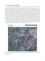
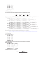
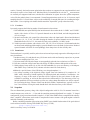
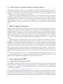
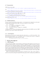
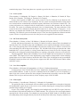
GMRT Observer’s Manual
Dharam Vir LAL
dharam AT ncra DOT tifr DOT res DOT in
November 18, 2013
Contents
1 An Overview of the GMRT
3
2 Specifications of the GMRT
2.1 Antennas . . . . . . . . . . . . . . . . . . . . . . . . . . . . .
2.1.1 Observing Frequency Bands . . . . . . . . . . . . . . .
2.1.2 Bandwidth . . . . . . . . . . . . . . . . . . . . . . . .
2.1.3 Resolution . . . . . . . . . . . . . . . . . . . . . . . .
2.1.4 Field of View . . . . . . . . . . . . . . . . . . . . . . .
2.1.5 Primary Beam . . . . . . . . . . . . . . . . . . . . . .
2.1.6 Sensitivity . . . . . . . . . . . . . . . . . . . . . . . .
2.2 System Parameters . . . . . . . . . . . . . . . . . . . . . . . .
2.3 Data Rates . . . . . . . . . . . . . . . . . . . . . . . . . . . . .
2.4 Subarrays . . . . . . . . . . . . . . . . . . . . . . . . . . . . .
2.5 Pointing Accuracy and Pointing Correction . . . . . . . . . . .
2.6 Polarisation . . . . . . . . . . . . . . . . . . . . . . . . . . . .
2.7 GSB Configurations . . . . . . . . . . . . . . . . . . . . . . . .
2.7.1 Correlator . . . . . . . . . . . . . . . . . . . . . . . . .
2.7.2 Beamformer . . . . . . . . . . . . . . . . . . . . . . .
2.8 Snapshots . . . . . . . . . . . . . . . . . . . . . . . . . . . . .
2.9 GMRT Calibrators: Amplitude, Bandpass and Phase Calibration
.
.
.
.
.
.
.
.
.
.
.
.
.
.
.
.
.
.
.
.
.
.
.
.
.
.
.
.
.
.
.
.
.
.
.
.
.
.
.
.
.
.
.
.
.
.
.
.
.
.
.
.
.
.
.
.
.
.
.
.
.
.
.
.
.
.
.
.
.
.
.
.
.
.
.
.
.
.
.
.
.
.
.
.
.
.
.
.
.
.
.
.
.
.
.
.
.
.
.
.
.
.
.
.
.
.
.
.
.
.
.
.
.
.
.
.
.
.
.
.
.
.
.
.
.
.
.
.
.
.
.
.
.
.
.
.
.
.
.
.
.
.
.
.
.
.
.
.
.
.
.
.
.
.
.
.
.
.
.
.
.
.
.
.
.
.
.
.
.
.
.
.
.
.
.
.
.
.
.
.
.
.
.
.
.
.
.
.
.
.
.
.
.
.
.
.
.
.
.
.
.
.
.
.
.
.
.
.
.
.
.
.
.
.
.
.
.
.
.
.
.
.
.
.
.
.
.
.
.
.
.
.
.
.
.
.
.
.
4
. 4
. 4
. 4
. 4
. 4
. 5
. 5
. 6
. 7
. 7
. 7
. 7
. 7
. 8
. 8
. 8
. 10
3 Radio Frequency Interference
10
4 Observing with the GMRT
4.1 Regular Observing Proposals for TAC . . . . . . . . . . . . . . . . . . .
4.1.0.1 Proposing for GMRT Observations: Checklist . . . . .
4.1.1 TAC Approved Proposals . . . . . . . . . . . . . . . . . . . . . .
4.1.2 Director’s Discretionary Time . . . . . . . . . . . . . . . . . . .
4.2 Planning the Observing Run . . . . . . . . . . . . . . . . . . . . . . . .
4.2.1 Continuum / Spectral-line . . . . . . . . . . . . . . . . . . . . .
4.2.1.1 Interferometric Observations: Pre-observation Checklist
4.2.1.2 Observatory Supported Modes . . . . . . . . . . . . .
4.2.2 Pulsar . . . . . . . . . . . . . . . . . . . . . . . . . . . . . . . .
4.2.2.1 Pulsar Observations: Pre-observation Checklist . . . .
4.2.3 Data Access . . . . . . . . . . . . . . . . . . . . . . . . . . . . .
1
.
.
.
.
.
.
.
.
.
.
.
.
.
.
.
.
.
.
.
.
.
.
.
.
.
.
.
.
.
.
.
.
.
.
.
.
.
.
.
.
.
.
.
.
.
.
.
.
.
.
.
.
.
.
.
.
.
.
.
.
.
.
.
.
.
.
.
.
.
.
.
.
.
.
.
.
.
.
.
.
.
.
.
.
.
.
.
.
.
.
.
.
.
.
.
.
.
.
.
.
.
.
.
.
.
.
.
.
.
.
10
10
11
11
11
12
12
12
12
12
13
14
4.3
4.4
4.2.3.1 GMRT Data Archive . . . . . . . . . . . . . . . . . . . . . . . . . . . . . 14
GMRT User Tool . . . . . . . . . . . . . . . . . . . . . . . . . . . . . . . . . . . . . . . . 14
Converting the Native LTA Format to FITS Format . . . . . . . . . . . . . . . . . . . . . . 14
5 Analysing Data from the GMRT: Straw Man Recipe
5.1 Setting-up NRAO AIPS . . . . . . . . . . . . . .
5.2 Loading Data . . . . . . . . . . . . . . . . . . .
5.3 Indexing . . . . . . . . . . . . . . . . . . . . . .
5.3.1 HEADER Information . . . . . . . . . .
5.4 Data Editing / FLAGging / Viewing . . . . . . .
5.5 Gain Calibration . . . . . . . . . . . . . . . . . .
5.5.1 SETJY . . . . . . . . . . . . . . . . . .
5.5.2 CALIB . . . . . . . . . . . . . . . . . .
5.5.3 GETJY . . . . . . . . . . . . . . . . . .
5.5.4 CLCAL . . . . . . . . . . . . . . . . . .
5.5.5 Bandpass Calibration . . . . . . . . . . .
5.5.6 CLCAL . . . . . . . . . . . . . . . . . .
5.6 Saving your Tables . . . . . . . . . . . . . . . .
5.7 Splitting the Target Source . . . . . . . . . . . .
5.8 Imaging: Continuum . . . . . . . . . . . . . . .
5.9 Imaging: Spectral-line . . . . . . . . . . . . . .
5.9.1 Continuum Image . . . . . . . . . . . .
5.9.2 Subtracting the Continuum . . . . . . . .
5.9.3 Making a Spectral Cube . . . . . . . . .
5.9.4 Extracting the Spectrum . . . . . . . . .
.
.
.
.
.
.
.
.
.
.
.
.
.
.
.
.
.
.
.
.
.
.
.
.
.
.
.
.
.
.
.
.
.
.
.
.
.
.
.
.
.
.
.
.
.
.
.
.
.
.
.
.
.
.
.
.
.
.
.
.
.
.
.
.
.
.
.
.
.
.
.
.
.
.
.
.
.
.
.
.
.
.
.
.
.
.
.
.
.
.
.
.
.
.
.
.
.
.
.
.
.
.
.
.
.
.
.
.
.
.
.
.
.
.
.
.
.
.
.
.
.
.
.
.
.
.
.
.
.
.
.
.
.
.
.
.
.
.
.
.
.
.
.
.
.
.
.
.
.
.
.
.
.
.
.
.
.
.
.
.
.
.
.
.
.
.
.
.
.
.
.
.
.
.
.
.
.
.
.
.
.
.
.
.
.
.
.
.
.
.
.
.
.
.
.
.
.
.
.
.
15
15
15
15
16
16
16
16
16
16
17
17
17
17
17
17
18
18
18
18
18
6 Miscellaneous
6.1 Making the Observations: Logistics . . . . . . . . . . . . . . . . . . . . .
6.1.1 Accommodation, Travel & Help for Visitors to the GMRT / NCRA
6.1.1.1 Absentee Observing . . . . . . . . . . . . . . . . . . . .
6.2 Tools . . . . . . . . . . . . . . . . . . . . . . . . . . . . . . . . . . . . . .
6.2.1 A Flagging and Calibration Pipeline . . . . . . . . . . . . . . . . .
6.3 Publication Guidelines . . . . . . . . . . . . . . . . . . . . . . . . . . . .
6.3.1 Acknowledging the GMRT . . . . . . . . . . . . . . . . . . . . . .
6.3.2 Dissertations . . . . . . . . . . . . . . . . . . . . . . . . . . . . .
6.4 Key Personnel . . . . . . . . . . . . . . . . . . . . . . . . . . . . . . . . .
6.5 Documentation . . . . . . . . . . . . . . . . . . . . . . . . . . . . . . . .
6.6 Modification History . . . . . . . . . . . . . . . . . . . . . . . . . . . . .
6.6.1 Acknowledgments . . . . . . . . . . . . . . . . . . . . . . . . . .
.
.
.
.
.
.
.
.
.
.
.
.
.
.
.
.
.
.
.
.
.
.
.
.
.
.
.
.
.
.
.
.
.
.
.
.
.
.
.
.
.
.
.
.
.
.
.
.
.
.
.
.
.
.
.
.
.
.
.
.
.
.
.
.
.
.
.
.
.
.
.
.
.
.
.
.
.
.
.
.
.
.
.
.
.
.
.
.
.
.
.
.
.
.
.
.
.
.
.
.
.
.
.
.
.
.
.
.
19
19
19
19
19
19
20
20
20
20
21
21
21
7 Ongoing Developments
7.1 GMRT Upgrades . . . . . . .
7.1.1 Servo System . . . . .
7.1.2 RF Front-end Systems
7.1.3 Low Noise Amplifier .
7.1.4 Fiber-Optics . . . . .
7.1.5 Back-end Systems . .
.
.
.
.
.
.
.
.
.
.
.
.
.
.
.
.
.
.
.
.
.
.
.
.
.
.
.
.
.
.
.
.
.
.
.
.
.
.
.
.
.
.
.
.
.
.
.
.
.
.
.
.
.
.
21
21
22
22
22
22
23
.
.
.
.
.
.
.
.
.
.
.
.
.
.
.
.
.
.
.
.
.
.
.
.
.
.
.
.
.
.
.
.
.
.
.
.
.
.
.
.
.
.
2
.
.
.
.
.
.
.
.
.
.
.
.
.
.
.
.
.
.
.
.
.
.
.
.
.
.
.
.
.
.
.
.
.
.
.
.
.
.
.
.
.
.
.
.
.
.
.
.
.
.
.
.
.
.
.
.
.
.
.
.
.
.
.
.
.
.
.
.
.
.
.
.
.
.
.
.
.
.
.
.
.
.
.
.
.
.
.
.
.
.
.
.
.
.
.
.
.
.
.
.
.
.
.
.
.
.
.
.
.
.
.
.
.
.
.
.
.
.
.
.
.
.
.
.
.
.
.
.
.
.
.
.
.
.
.
.
.
.
.
.
.
.
.
.
.
.
.
.
.
.
.
.
.
.
.
.
.
.
.
.
.
.
.
.
.
.
.
.
.
.
.
.
.
.
.
.
.
.
.
.
.
.
.
.
.
.
.
.
.
.
.
.
.
.
.
.
.
.
.
.
.
.
.
.
.
.
.
.
.
.
.
.
.
.
.
.
.
.
.
.
.
.
.
.
.
.
.
.
.
.
.
.
.
.
.
.
.
.
.
.
.
.
.
.
.
.
.
.
.
.
.
.
.
.
.
.
.
.
.
.
.
.
.
.
.
.
.
.
.
.
.
.
.
.
.
.
.
.
.
.
.
.
.
.
.
.
.
.
.
.
.
.
.
.
.
.
.
.
.
.
.
.
.
.
.
.
.
.
.
.
.
.
.
.
.
.
.
.
.
.
.
.
.
.
.
.
.
.
.
.
.
.
.
.
.
.
.
.
.
.
.
.
.
.
.
.
.
.
.
.
.
.
.
.
.
.
.
.
.
.
.
.
1 An Overview of the GMRT
The Giant Metrewave Radio Telescope (GMRT) is located near Khodad village, which is about 80 km north
of Pune. The GMRT consists of an array of 30 antennae, each of 45 m diameter, spread over a region of
25 km diameter. Amongst the multi-element earth rotation aperture synthesis telescopes operating at meter
wavelengths, the GMRT has the largest collecting area. The interferometer has a hybrid configuration with
14 of its 30 antennas located in a central compact array with size ∼1.1 km and the remaining antennas distributed in a roughly ‘Y’ shaped configuration, giving a maximum baseline length of ∼25 km. The baselines
obtained from antennas in the central square are similar in length to the VLA D-array configuration, while
the baselines between the arm antennas are comparable in length to the baseline lengths between VLA Aarray and VLA B-array configurations. Hence, a single observation with the GMRT samples the (u, v) plane
adequately on both short and long baselines with reasonable sensitivities. The GMRT can also be configured in array mode, where it acts as a single dish by adding the signals from individual dishes. This mode of
operation is used for studying compact objects like pulsars, which are effectively point sources even for the
largest interferometric baselines. The maximum instantaneous operating bandwidth at any frequency band
is 33 MHz. Each antenna provides signals in two orthogonal polarisations, which are processed through a
heterodyne receiver chain and brought to the central receiver building, where they are converted to baseband
signals and fed to the digital back-end consisting of correlator and pulsar receiver.
screen, use the "Print" link next to the map.
Imagery ©2013 Cnes/Spot Image, DigitalGlobe, Map data ©2013 Google -
Figure 1: Location of the GMRT array as seen on the Google-maps (latitude and longitude are provided in
Section 2.1 below).
3
2 Specifications of the GMRT
2.1
Antennas
The GMRT antennas are alt-azimuth mounted parabolic prime-focus dishes. While the dishes can go down
to an elevation of 16◦ , at present, the elevation limit has been set at 17◦ , giving a declination coverage from
−53◦ to +90◦ . The slew speed of the antennas is 20◦ min−1 on elevation axis and 30◦ min−1 on azimuth
axis, and they are not operated when winds are higher than 40 km h−1 . The reference antenna, C02 of the
array is located at
latitude = 19.1◦ N ,
longitude = 74.05◦ E,
altitude = 588 m.
2.1.1 Observing Frequency Bands
There is a rotating turret at the focus on which the different feeds are mounted. The feeds presently available
are the 150, 325, 610/235 and the 1000−1450 MHz feeds. The 1000−1450 MHz feed, L-band feed is
subdivided into 1060, 1170, 1280 and 1390 MHz sub-bands. The reflecting surface is formed by wire
mesh and the efficiency of the antennas varies from 60% to 40%, from the lowest to the highest frequency.
Both the orthogonal polarisations are brought to the control room from each antenna. The polarisations are
circular for all feeds except the 1420 MHz feeds, which are linear. The 610 MHz and 235 MHz feeds are
coaxial, allowing simultaneous dual frequency observations to be carried out at these two frequency bands,
albeit for only one polarisation per band.
2.1.2 Bandwidth
The new GMRT Software Backend (GSB) supports a maximum bandwidth of 32 MHz. Users should consult
the observatory regarding usable RF bandwidth at the lower frequencies because of RFI. For 150 MHz and
235 MHz, the recommended IF bandwidth is 6 MHz; however, 16 MHz is also usable, albeit with some
caution.
2.1.3 Resolution
The approximate synthesized beam size (full width at half-maximum) for a full synthesis observation at
each of the observing bands is given below:
150 MHz: ∼20′′
235 MHz: ∼13′′
325 MHz: ∼9′′
610 MHz: ∼5′′
1280 MHz: ∼2′′
2.1.4 Field of View
The field of view, diffraction-limited response of the individual antennas is
θ ≃ 85.2 ×
325 GHz
,
ν
where θ, the half-power beam-width is in arcmin and ν is the frequency. These are
150 MHz: 186′ ±6′
4
235 MHz: 114′ ±5′
325 MHz: 81′ ±4′
610 MHz: 43′ ±3′
1280 MHz: 26.2′ ±2′
2.1.5 Primary Beam
The coefficients of an eighth order polynomial fit to the antenna primary beam
1+(
a
b
c
d
)x2 + ( 7 )x4 + ( 10 )x6 + ( 13 )x8 ,
3
10
10
10
10
where a, b, c and d are PBPARM(3), PBPARM(4), PBPARM(5) and PBPARM(6), respectively. These can
be directly plugged into AIPS task PBCOR are
150 MHz: PBPARM(1) = 0.1; PBPARM(2) = 1; PBPARM(3) = −4.04;
PBPARM(4) = 76.2; PBPARM(5) = −68.8; PBPARM(6) = 22.03; PBPARM(7) = 0
235 MHz: PBPARM(1) = 0.1; PBPARM(2) = 1; PBPARM(3) = −3.366;
PBPARM(4) = 46.159; PBPARM(5) = −29.963; PBPARM(6) = 7.529; PBPARM(7) = 0
325 MHz: PBPARM(1) = 0.1; PBPARM(2) = 1; PBPARM(3) = −3.397;
PBPARM(4) = 47.192; PBPARM(5) = −30.931; PBPARM(6) = 7.803; PBPARM(7) = 0
610 MHz: PBPARM(1) = 0.1; PBPARM(2) = 1; PBPARM(3) = −3.486;
PBPARM(4) = 47.749; PBPARM(5) = −35.203; PBPARM(6) = 10.399; PBPARM(7) = 0
1280 MHz: PBPARM(1) = 0.1; PBPARM(2) = 1; PBPARM(3) = −2.27961;
PBPARM(4) = 21.4611; PBPARM(5) = −9.7929; PBPARM(6) = 1.80153; PBPARM(7) = 0
More details such as the fitted polynomial, methodology, etc. are available at
http://www.ncra.tifr.res.in:8081/˜ngk/primarybeam/beam.html .
2.1.6 Sensitivity
The system temperature is
150 MHz: 615 K†
235 MHz: 237 K†
325 MHz: 106 K
610 MHz: 102 K
1280 MHz: 73 K
† The system temperature measurements are with Solar attenuator switched on,
and the antenna gain is
150 MHz: 0.33 K Jy−1 Antenna−1
235 MHz: 0.33 K Jy−1 Antenna−1
325 MHz: 0.32 K Jy−1 Antenna−1
610 MHz: 0.32 K Jy−1 Antenna−1
1280 MHz: 0.22 K Jy−1 Antenna−1
The RMS noise sensitivity equation is,
√
2 k Tsys
p
∆S =
,
ηa ηc A (nb ) nIF ∆ν τ
5
and the on-source integration time τ is computed via,
√
2 k Tsys 2
1
τ =(
) ×
∆S × ηa ηc A
(nb ) nIF ∆ν
where ∆S is the required RMS noise (Jy), Tsys is the system temperature (K), and [(ηa A)/(2k)] = G is
the antenna gain (K/Jy), where ηa (see Section 2.1.1) and ηc (≃ 1) being aperture and correlator efficiencies
respectively. A is the geometrical area of the antenna, nb is the number of baselines, nIF is the number of IF
channels, and ∆ν (Hz) is the bandwidth of each sideband (or channel width for spectral line observations).
nIF = npol + nSB , where npol is the number of polarisations (2 for the GMRT) and nSB is the number of
sidebands.
2.2
System Parameters
Below in the Table 1, we list the system parameters. It also lists best RMS sensitivities and typical dynamic
ranges achieve in a mapped field, which are known to us.
Primary beam (HPBW, arcmin)
151
186 ±6
235
114 ±5
Frequency (MHz)
325
610
81 ±4
43 ±3
1420
(24 ±2)×(1400/f )
System temperature (Tsystem , K)
Receiver temperature (TR )
Typical Tsky (off Galactic plane)
Typical Tground
Tsystem (= TR + Tsky + Tground )
295†
308
12
615
106†
99
32
237
53
40
13
106
60
10
32
102
45
4
24
73
Antenna gain (K Jy−1 Antenna−1 )
0.33
0.33
0.32
0.32
0.22
Synthesized beam (FWHM)
− Full array (arcsec)
− Central square (arcsec)
20
420
13
270
9
200
5
100
2
40
Largest detectable structure (arcmin)
68
44
32
17
7
Usable frequency range
− observatory default (MHz)
− allowed by electronics (MHz)
150–156
130–190
236–244
230–250
305–345
305–360
580–640
570–650
1000–1450
1000–1450
Fudge factor (actual to estimated time)
− for short observations
− for long observations#
10
5
5
2
2
2
2
1
2
1
Best RMS sensitivities achieved (mJy)‡
0.7
0.25
0.04
0.02
0.03
Typical dynamic range achieved
>1500
>1500
>1500
>2000
>2000
† With default solar attenuator (14 dB).
# For spectral observations fudge factor is close to 1.
‡ So far known to us!
Table 1: Measured system parameters of the GMRT
6
2.3
Data Rates
For the correlator configurations discussed in Section 2.7, integration time ∆t, and recording both self and
cross correlation coefficients, the data rate is
= 1.86 × [
2 sec
Nant × (Nant + 1)
×(
)] MB sec−1 ,
(30 × 31)
∆t
= 3.35 × [
Nant × (Nant + 1)
2 sec
×(
)] GB hr−1 ,
(30 × 31)
∆t
which corresponds to ∼0.1 TB day−1 when using the full 30-element array with 2 sec integrations, 2 (RR
and LL) total intensity polarisations and 512 spectral channels.
2.4
Subarrays
GMRT supports multiple subarrays for users, where the array is divided into smaller groups of antennas. It
can be configured in array mode, where it acts as a single dish by adding the signals from individual dishes.
Note that up to a maximum of five subarrays are possible at any given time and it is not possible to have
different correlator settings for these subarrays. This mode of operation is used for studying compact objects
like pulsars, which are effectively point sources even for the largest interferometric baselines.
2.5
Pointing Accuracy and Pointing Correction
The typical pointing accuracy of a GMRT antenna is 1 arcsec and the typical tracking accuracy is 10 arcmin. A pointing model has been in use since observing cycle-15, which can be applied online during the
observations; it updates the antenna pointing offsets every half an hour or so during an observing run, using
commands included in the user’s observe file. Elevation dependent offsets are seen in a few antennas,
which can again be corrected using a pointing model. If a user does not want to apply the dynamic pointing
model, the control room should be informed before the start of the observing run.
2.6
Polarisation
Polarisation observations are now possible using GMRT and several users have carried out full polar observations at 610 MHz. Interested users could look at the following article
http://arxiv.org/abs/1309.4646 .
Despite the on-axis instrumental polarisation at GMRT being of large amplitude and highly frequencydependent, this article demonstrates the viability of the GMRT for full-polarisation, wide-field spectropolarimetry.
2.7
GSB Configurations
The current GMRT Software Back-end (GSB) offers relatively more options as compared to its earlier
hardware counterpart. Current status and latest news about the GSB can be found at
http://gmrt.ncra.tifr.res.in/gmrt_hpage/sub_system/gmrt_gsb .
Table 2 presents the available modes of the back-end. Briefly, from cycle-20 onwards the GSB is the backend at the observatory, the older hardware back-ends have been decommissioned, and the details of available
modes are as follows:
The new GSB back-end supports a maximum bandwidth of 32 MHz. However, users should consult
the observatory regarding usable RF bandwidth at the lower frequencies because of RFI. For 150 MHz and
235 MHz, the recommended IF bandwidth is 6 MHz; however, 16 MHz is also usable, albeit with some
7
caution. Currently, the interferometre polarisation observations are supported on an experimental basis and
the analysis requires a lot of hard work. Walsh and Noise Cal modulation for real time Tsys measurements
are currently not supported and hence, absolute flux calibration in regions where the system temperature
varies (like the galactic plane) is not automatic. Normal integration times used are 8 or 16 s but more rapid
sampling (down to 2 s) can be done, subject to the availability of enough disk space for recording the larger
data volume. Users requiring such modes should consult the ‘Operations” group at the observatory.
2.7.1 Correlator
It presently supports the following modes of interferometric observations:
i Full bandwidth, non-polar and full polar interferometric observations in the “16 MHz” and “32 MHz”
modes, with a choice of 256 or 512 spectral channels across the full band, and with integration time
of 2 sec or larger.
ii Spectral zoom modes (for spectral line observations) where the input band is filtered and decimated
by factors 4, 8, 16, 32, 64, 128 while keeping the number of spectral channels across the reduced
bandwidth fixed at 256 or 512 – this mode will only work within the “16 MHz” mode.
iii Variable spectral resolution, with a choice of 64, 128, 256, 512 or 1024 (note: 1024 channel mode has
not been tested and debugged thoroughly) spectral channels across the band of observation. Reduced
spectral channels will allow for correspondingly faster dump times for the visibility data.
2.7.2 Beamformer
The beamformer is especially used for pulsar observations and it presently supports the following modes of
array beamformer:
i Incoherent array (IA) and phased array (PA) beam modes with total intensity output; here at present
the fastest sampling time is 60 µsec.
ii PA beam mode with full polar output at correspondingly reduced time resolutions (see Table 2).
iii Full time resolution voltage beam data with facility for offline coherent dedispersion of the same.
iv Multi-subarray beam modes (IA or PA) with full bandwidth, for up to two subarrays, with independent GMRT Array Combiner (GAC) antenna selection control for each subarray.
Additional, a special feature of the GSB being, raw voltage dump data, i.e.,
v raw voltage recording of the digitized voltage signals from each antenna (4 bit samples) for “16
MHz” mode, followed by limited capability for offline playback and correlation / beamformer – the
frequency of usage of this mode of operation will be restricted by the total volume of disk space
available for recording, as well as the time taken for the offline analysis. The observatory offers very
limited capabilities for long-term back-up of the raw voltage dump data and the user will be responsible for clearing the large volumes of data from the disks within a stipulated time, typically a week or
less. Users desirous of using this mode should check with the observatory well in advance.
2.8
Snapshots
The two-dimensional geometry along with a hybrid configuration with 14 of its 30 antennas located in a
central compact array with size ∼1.1 km and the remaining antennas distributed in a roughly ‘Y’ shaped
configuration, giving a maximum baseline length of ∼25 km of the GMRT allows a snapshot mode whereby
short, “snapshot” observations can be made to map detailed source structure with good angular resolution
and with reasonably good sensitivity.
Before considering snapshot observations using GMRT, users should first determine if the goals desired
can be achieved with the existing TIFR GMRT Sky Survey (TGSS),
http://tgss.ncra.tifr.res.in/ ,
which is an all sky survey at 150 MHz.
8
!
!
"#
$ #
%& '
*+,(-,-
*+
.(+,+.-
(-#
(-,-
(-
.(+,+.-
+,/,011
(+0
21.,(,+11
-/,*+
21+.,21.,(11
3
4
*+#
*+,(-,-
*+
.(+5,+.- +,/,011
3
4
(-#
(-,-
(-
.(+,+.-
+,/,011
+ $
#) 3 6
(-
7
#
(-,-
(-!"
"8/,0,(-11(+0
1/,+,(,
21.,21+.921(+.
.(+,+.-
+,/,011
* ) #
*+#
*+,(-,-
*+
.(+,+.-
:);
:
)(,+,/
(-#
(-,-
(-!""8/,0,(-
1/,+,(
.(+,+.-
:);
:
)(,+,/
*+#
*+,(-,-
*+
.(+,+.-
:);
:
)(,+,/
(-#
(-,-
(-!""8/,0,(-
1/,+,(
.(+,+.-
:);
:
)(,+,/
3
4
(-#
(-,-
(-
.(+,+.-
:);
:
)(,+,/
<
#
*+#
*+,(-,-
*+
.(+,+.-
(.=
<
#
(-#
(-,-
(-
.(+,+.-
*2=
'7
$
# (-,-
(-
( $
#) %
#
*+#
:
/ '7>#
+,/,011
*2/
# !
"
##################################################################################
$%&'())*+,*-).*/ -0
$ 1 2)
$3$
##################################################################################
345 .-(.-,(.- 444
333 .-(.-,(.- 444
33 0
-(.-,(0 444
33366 0
-(.-,(0 444
##################################################################################
4444445 .-(.-,(.- 444
4444433 .-(.-,(.- 444
444443 0
-(.-,(0 67"8)*.
444443 0
-(.-,(0 67"8)*.
##################################################################################
9:
;<
0.
7";3;4='>
45;3='>
Table 2: Available modes of the GSB for continuum, spectral, pulsar and raw-dump observations. All
details, including standard-operating-procedure, etc. are available at GSB-SOP.
9
2.9
GMRT Calibrators: Amplitude, Bandpass and Phase Calibration
The flux density calibrators, 3C 48 (0137+331, J2000), 3C 147 (0542+498, J2000) and 3C 286 (or 1331+305,
J2000) are used for both, amplitude and bandpass calibration. Together these three calibrators almost cover
the entire 24 hr observing run. The flux density scale used for for the observing bands at GMRT is based on
the Baars et al. (1977 Astron. Astrophys., 61, 99) scale.
A suitable list of phase calibrators selected from the complete VLA calibrator list that are appropriate
for GMRT is being collated at 610 and 240 MHz. Once it is ready, it would be made available. Till then,
users can consult the VLA calibrator list for appropriate phase calibrator for their observation. Since the
mapped field-of-view (Section 2.1.4) are larger at low frequencies, users should map the calibrator field and
use these solutions, instead of assuming it to be a field with only one dominant point source at the phase
centre.
3 Radio Frequency Interference
Radio-frequency interference (RFI) signals are among the main factors limiting the performance of radio
telescopes. RFI constricts the available frequency space, effectively increases system noise and corrupts
calibration solutions. The effect is particularly strong at frequencies below 1 GHz. Although, the RFI environment at GMRT is fairly decent, especially at frequencies below 235 MHz band it can be quite alarming.
While the strongest source in a field is typically only a few Jy, the RFI can occasionally reach several hundred Jy in some channels in the 150 and 235 MHz bands. However broadband RFI of up to several tens
of Jy causes even more damage: currently available tools, including the AIPS task FLGIT provide some
solution.
As mentioned above, the RFI environment can be bad at 150 MHz and is sometimes a problem at
235 MHz; the situation is usually better at night time and on weekends. (For these two bands, it is recommended to use the solar attenuators in the common box, to minimize the possibilities of saturating the
downstream electronic chain due to RFI.) Observations at 325 MHz can be hampered sometimes due to RFI
from nearby aircraft activity, especially during day time. Due to increasing interference from mobile phone
signals around 950 MHz, the all-pass mode at 1400 MHz band is no longer supported as an official mode,
and consequently observations below 1000 MHz in this band are not supported. Even for the lowest of the
4 sub-bands of the 1400 MHz band (covering 1060 ± 60 MHz), the user is advised to check for effects of
RFI.
Please refer to Sections 2.1.2 and 4.2.1.2 for usable bandwidth and default settings, respectively. Users
are also informed that since cycle-21, night time scintillation has been occasionally seen, even at the 1400
MHz band, and the probability of scintillation is higher close to the equinoxes.
4 Observing with the GMRT
4.1
Regular Observing Proposals for TAC
The GMRT Time Allocation Committee (GTAC) invites proposals for two Cycles (April to September and
October to March). The deadline for receiving these proposals is 17:00 HRS IST (UTC+5.5 hrs), January
15, and July 15. All proposals are to be submitted online via the NCRA Archive and Proposal Management
System (NAPS), available at
http://naps.ncra.tifr.res.in ,
which provides a password authenticated, web browser based interface for proposal submission. Note that
proposal may be submitted only by the PI. All co-I’s also need to be registered users of the system. All proposals are processed by GTAC with external refereeing as needed with inputs from the GMRT Observatory
on technical issues and the proposers are sent intimations of the time allocation. The call for proposals, the
10
status of the GMRT, and a set of guidelines for GMRT users can be found at
http://www.ncra.tifr.res.in/ncra/gmrt/gtac .
Additionally, frequently asked questions on GMRT proposal submission are available at
http://www.ncra.tifr.res.in:8081/˜yogesh/proposalfaq.html ,
and the quick-start guide to GMRT proposal submission is available at
http://www.ncra.tifr.res.in:8081/˜yogesh/quickstartguide.html .
After a proposal has been allotted time and scheduled, further queries regarding travel logistics (see
Section 6.1) can be addressed to the “Secretary - Operations”
(secr-ops AT ncra DOT tifr DOT res DOT in).
Any queries related to the observing schedule should be sent to
gmrtschedule AT ncra DOT tifr DOT res DOT in ,
and regarding other aspects of the observations should be sent to
gmrtoperations AT ncra DOT tifr DOT res DOT in .
In the event of potential overlap of interests of different proposers, GTAC will try and encourage collaboration or sharing of data by bringing the concerned individuals into contact with each other.
Note that starting from 2012, GMRT has entered into an intensive phase of the ongoing upgrade (see
Section 6), and this requires additional day time slots for engineering activity. The observatory tries its
best to maintain the availability of 26 antennas for all the scientific observations. Some of the existing
observation modes and available flexibilities of settings for observations may be partially affected by the
changes implemented as part of the upgrade activities. In the regard, the users are advised to read the
GMRT status document, available at
http://www.ncra.tifr.res.in/ncra/gmrt/gtac ,
which is updated at every proposal deadline.
4.1.0.1 Proposing for GMRT Observations: Checklist
i ’Register’ and ’login’ at the
http://naps.ncra.tifr.res.in ,
ii choose ’Create Proposal’ and follow necessary steps.
iii Remember to attach a self-contained ’Scientific Justification’ not exceeding 3000 words. Preprints
or reprints will be ignored, unless reporting previous GMRT observations. A brief status report (not
exceeding 150 words) on each previous proposal should be appended to the scientific justification.
Note: when your proposal is scheduled, the contents of the cover sheets become public information. Any
supporting pages are for refereeing purpose only.
4.1.1 TAC Approved Proposals
4.1.2 Director’s Discretionary Time
In addition to regular GTAC proposals, users can also avail
i Target of Opportunity: Target of Opportunity (TOO) time is primarily intended for short lived, unexpected/
unpredicted phenomena or time dependent astronomical phenomena.
ii Exploratory Proposals: Here, the time is primarily meant for pilot observations or feasibility studies
which might lead to future GTAC proposals and confirmatory observations.
Both types of time allocation are subject to availability of time and will be evaluated on the basis of scientific merit by the relevant referees, and are cleared by the Centre Director, NCRA. Requests for allocation
of TOO and DDT should also be submitted using the NAPS interface, code “DDT”. Such observations will
be scheduled in the empty “white” slots
(http://www.ncra.tifr.res.in:8081/˜gmrtoperations/gtac/request.html),
11
without affecting the scheduled GTAC observations, as far as possible. the guidelines followed at the observatory for allocating these “white” slots are available at
http://www.ncra.tifr.res.in/ncra/gmrt/gtac .
4.2
Planning the Observing Run
If you are ready to observe, visit the following site for preparing your observations.
http://www.ncra.tifr.res.in/gmrt_hpage/Users/Help/help.html .
Also check that the following tasks (see Section 4.2.1.1 and 4.2.2.1) have been accomplished:
4.2.1 Continuum / Spectral-line
From cycle-20 onwards, the GSB is the only back-end available at the GMRT. The older, hardware backends have been decommissioned. All 30 antennas are in use and feeds for all frequencies are available. At
a given time, the observatory will try to make at least 26 antennas available for any observation. Programs
that critically depend on the short spacing antennas (C05, C06 and C09, with ∼ 100 m separation) must
indicate this in the GTAC proposal. Rotation of the feed system to change the frequency of observation is
now possible fairly routinely, and requires about 2 hours time for rotation and for set-up at the new frequency
of operation, including antenna pointing.
Section 2.1.6 gives the measured system parameters of the GMRT antennas and some useful numbers
for estimating the required observation time. Additional information can be found at
http://www.ncra.tifr.res.in/ncra/gmrt/gtac .
4.2.1.1 Interferometric Observations: Pre-observation Checklist
• contacted the observing assistant (the Operator) who would assist and run your observations.
• identified/selected a suitable bandpass calibrator
• flux density calibrator
• phase calibrator
• checked that all sources are visible during observing time
• prepared a source file in the right format
• prepared a command file using
http://gmrt.ncra.tifr.res.in/gmrt_hpage/Users/Help/sys/setup.html
and that this has been checked by the GMRT operator.
• calculated how much data the observations will generate, and obtained enough disk space to accommodate this. (Operator’s too warn you of this!)
4.2.1.2 Observatory Supported Modes Below in the Table 3, we list the default settings for a continuum observations at a given frequency, and system parameters, including usable frequency recommended/available,
respectively.
4.2.2 Pulsar
The GSB beamformer/pulsar receiver allows incoherent array (IA) and phased array (PA) mode observations using all the 30 antennas, with a maximum bandwidth of 32 MHz.
i For the IA mode observations, the actual number of antennas that can be added depends on the quality of the signals from the antennas, including effects of receiver instabilities and RFI. These effects
vary with time, the radio band being used and depends on the choice of antennas. i.e. from central
square antennas to arm antennas. Due to the current limitations of the data acquisition system, since
observing cycle-20, the fastest sampling achievable in the IA mode is 30 µsec and 61 µsec for the 256
12
RF
(MHz)
150
235
325
610
1060
1170
1280
1390
DUAL
LO 1
(MHz)
218
304
255
540
990
1100
1210
1320
680/304
IF-BW
(MHz)
16
16
32
32
32
32
32
32
32/16
tpa
156
242
306
591
1041
1151
1261
1371
629
156
242
306
591
1041
1151
1261
1371
253
218
304
255
540
990
1100
1210
1320
680
218
304
255
540
990
1100
1210
1320
304
62
62
51
51
51
51
51
51
51
62
62
51
51
51
51
51
51
51
Table 3: Supported defaults for a typical continuum observation.
channels and 512 channels, for both, 16 or 32 MHz modes of the GSB.
ii For the PA mode of observations, there is an algorithm that can phase any selected number of available, working antennas using interferometric observations of a point source calibrator. The phasing
for central (∼ 14) antennas works well for time scales ranging from one hour to a few hours, depending on the operational frequency and the ionospheric conditions. For the arm antennas or for the
longer baselines, de-phasing can be more rapid.
iii Polarimetric pulsar observations are possible with the GSB, but instrumental polarisation effects for
the GMRT are not fully characterised and observers will therefore need to carry out their own calibration.
iv For total intensity, the fastest sampling rate currently supported is 30 µsec and 61 µsec for the 256
channels and the 512 channels, respectively, for both, 16 and 32 MHz modes of the GSB.
v For the polar mode, the fastest sampling times are slower by a factor of 4 than these numbers, i.e.,
122 µsec and 245 µsec for the 256 channels and the 512 channels, respectively for the corresponding
GSB modes. Here, both IA and PA modes are available with a time tagging facility that is accurate to
∼240 × 10−9 sec with respect to the GPS-clock and the timing observations can be carried out.
The format of the beamformer data from the GSB is identical to that provided by the older hardware pulsar
back-end. The final multi-channel data from the IA beamformer output can be recorded either on disk or
on tapes (SDLT or LTO). The PA data from the GSB can also be recorded on disk or tapes (SDLT or LTO).
User can choose either the total intensity signal or the four polarisations signal to record.
Additionally, the PA mode of the GSB also includes capability for recording the full time resolution
voltage beam data with a facility for off-line coherent dedispersion. Finally, the GSB also allows a mode
where the single IA and PA beams can be replaced by two IA beams or two PA beams, with independent
antenna selections for each. This facilitates simultaneous dual-frequency observations of pulsars using
the subarray mode (see Section 2.4) of the GMRT. Note that such observations involve special scheduling
considerations, due to feed rotations and related overheads.
A Pulsar observing manual, for more details, is available at
http://gmrt.ncra.tifr.res.in/gmrt_hpage/Users/Pulsar/PULSAR_MANUAL.pdf .
4.2.2.1 Pulsar Observations: Pre-observation Checklist
• contacted the observing assistant (the Operator) who would assist and run your observations.
• calibrator for gain equalisation @300 count (close to target, ph-cal will work, but > 5 Jy)
• perform phasing on the phase calibrator
• go to target pulsar
• configure IA+PA GAC
13
• start IA and/or PA ACQ (acquisition) + Process chain
• start data recording to the disk
4.2.3 Data Access
The data from the GMRT can be converted to FITS files using locally developed software, and analysed in
standard packages like AIPS (see Section 4.4). These can be backed up on DVDs or external hard disks,
written by Linux machines. Users are requested to bring their own media for backing up the data. Facilities
for analysing GMRT data are available both at the Observatory and at the NCRA, Pune. Users requiring
extensive computing facilities or large amounts of disk space for data storage or analysis should make their
requirements known well in advance.
The online archive contains all GMRT data since 2002 (Cycle-01), and will also serve the user community with GMRT data. The entire archive is now on disk, and is available via the Archive Access Tool at
https://naps.ncra.tifr.res.in/goa/mt/search/basicSearch .
Data from all standard observations with the GMRT will be made public 18 months after the date of observation, and the TOO observations will be made public three months after the date of observation.
4.2.3.1 GMRT Data Archive Since GMRT observing cycle-1 (year 2002) observations, the entire archive
is available via the web. The following url allows to view the data,
https://naps.ncra.tifr.res.in/goa/mt/search/basicSearch .
Presently this archive provide FITS (u, v) format files and native LTA format files. Data-base searches may
be made based on a large number of user-specified criteria and one can download data via ftp protocols.
Similar to all other observatories, GMRT data too are restricted to proprietary use by the proposing team for
a period of 18 months from the date of the last observation in a proposal.
4.3
GMRT User Tool
A GMRT User Tool (GUT) has been released for users. It is a graphical interface to several existing GMRT
software that are regularly used before observations (e.g. command file maker, rise and set time calculator),
during observations (e.g. ondisp for monitoring the antenna status etc) and after observations (e.g. tax,
gvfits) and includes a few other useful utilities. This can be accessed by saying gut at the UNIX prompt
on any computer at the observatory.
4.4
Converting the Native LTA Format to FITS Format
Assuming that telescope operators gave you your data in the the native LTA format, 01TST01 OBJ.lta file
– this file is in the raw telescope format, where lta stands for long term accumulation: programs available
at the observatory, e.g., XTRACT, TAX, etc. used for quick check of the data quality operate on the LTA
format. First run the program listscan to create “01TST01 OBJ.log” file. Edit the “log” file to select
normalisation type, a subset of the data, provide your favourite name (UVDATA.FITS) to the output file,
etc. Finally run gvfits (it provides UV data in J2000 epoch) on the edited log file. For example,
bash> listscan /PATH/DATE/01TST01_OBJ.lta
bash> vi 01TST01_OBJ.log
bash> gvfits 01TST01_OBJ.log
Note that these programs, e.g., listscan, gvfits, etc. are observatory based programmes, which are available
on all GTAC computing machines at GMRT and NCRA.
14
5 Analysing Data from the GMRT: Straw Man Recipe
Although one can use FLAGCAL to flag and calibrate GMRT data (see Section 6.2.1 for more details) and
move straight to Section 5.8 and perform imaging, here, we present a quick recipe for the analysis of GMRT
data from scratch using classic AIPS. The users program source is named PROG-SRC. The interferometer
phase is calibrated by observations of PH-CAL. The flux density scale and the bandpass is calibrated by
observing AMPBP-CAL. The data-file containing this observation is named as UVDATA.FITS containing
256 spectral channels at 610 MHz.
5.1
Setting-up NRAO AIPS
Classic AIPS is installed on all machines at the observatory. Or, alternatively install AIPS on your machine
from
http://www.aips.nrao.edu/index.shtml .
Next, for bourne shell,
bash> export FITS=/data/aips/FITS/
bash> source /data/aips/LOGIN.SH
or alternatively for csh/tsch shell
csh> setenv FITS /data/aips/FITS/
csh> source /data/aips/LOGIN.CSH
and start AIPS via
bash> /data/aips/START_AIPS
Typically at the AIPS prompt
> TASK ’taskname’
> INP to review the input parameters, called ADVERBS of ’taskname’
> GO runs the task ’taskname’
> EXPLAIN ’taskname’ prints helpful information on the terminal or on the line printer
> UCAT lists cataloged UV files
> MCAT lists cataloged map files
> GETNAME n assigns the INNAME, INCLASS, INSEQ and INTYPE values
corresponding to file with catalog no. ’n’
> ZAP delete a catalog entry and its extensions files
> RESTORE 0 initializes AIPS and restores defaults
> KLEENEX exit from AIPS wiping the slate kleen
5.2
Loading Data
TASK ’FITLD’; DATAIN ’FITS:UVDATA.FITS’; GO
Say, this makes the catalog no. 1.
5.3
Indexing
TASK ’INDXR’; GETN 1; CPARM(3) = 1; GO
This creates NX and CL (ver. 1) tables.
15
5.3.1 HEADER Information
.
GETN n; IMHE
It lists header information from the catalog file no. ’n’ selected. It also lists tables that have two letter
names, which are
HI Human readable history of things done to your data. Use AIPS task PRTHI to read it and task PRTAB
to read other tables.
AN Antenna location (and polarisation) tables.
NX Index into visibility file based source name and observation time.
SU Source table contains the list of sources observed and indexes into the frequency table. The flux densities of the calibration sources are entered into this table.
FQ Frequencies of observation and bandwidth with index into visibility data.
CL Calibration (ver. 1) table describing the antenna based gains. The goal of calibration is to create a
good CL ver. 2.
5.4
Data Editing / FLAGging / Viewing
TASK ’QUACK’; OPCODE ’BEG’; APARM 0.5; GO
This FLAGs the bad points at the beginning of each scan and creates a Flag Table (FG).
Again
TASK ’UVFLG’; ANTEN ?,0; TIMER ?; OUTFGVER=1; INP; GO
FLAGs bad UV data!
TASK ’LISTR’; OPTYP ’SCAN’; DOCRT 1; SOURC ’ ’; INP; GO
This LISTR task lists your UV data in a variety of ways and the above inputs show the summary of the
sources in the input data file.
5.5
Gain Calibration
5.5.1 SETJY
Enter the absolute flux density of the primary calibrator in the SU table,
TASK ’SETJY’; SOURCES ’AMPBP-CAL’, ’ ’; OPTYPE ’CALC’; GO
5.5.2 CALIB
Solve for the antenna based amplitudes and phases for AMPBP-CAL and PH-CAL,
TASK ’CALIB’; CALSOUR ’AMPBP-CAL’, ’PH-CAL, ’ ’; BCHAN Y; ECHAN Y;
REFANT X; SOLINT 2; GO
Here channel ’Y’ is a RFI-free channel from the dataset and antenna ’X’ is assumed to be ‘good’. This
will generate the solution SN table with ver. 1. The calibrated data can now be plotted using the AIPS task
UVPLT.
5.5.3 GETJY
Bootstrapping the flux density to the phase calibrator
TASK ’GETJY’; SOURCES ’PH-CAL’, ’ ’; CALSOUR ’AMPBP-CAL’, ’ ’; SNVER 0; GO
These values too are now written in the SU table.
16
5.5.4 CLCAL
Interpolate the gains
TASK ’CLCAL’; SOURCES ’AMPBP-CAL’; CALSOUR ’AMPBP-CAL’, ’ ’;
OPCODE ’CALI’; SNVER 0; INVER 0; GAINVER 1; GAINUSE 2; REFANT X; GO
Now the gains have been interpolated for the time instances of the program source. The solution (SN / CL)
tables can be plotted using the AIPS task SNPLT.
5.5.5 Bandpass Calibration
TASK ’BPASS’; CALSOUR ’AMPBP-CAL’, ’ ’; DOCAL 1; DOBAND −1; SOLINT 0;
REFANT X; BPASSPRM(5) 1; ICHANSEL Y Y 1 0; GO
The bandpass solutions (BP table) can be plotted using the AIPS task POSSM.
TASK ’POSSM’; APARM(8) = 2; NPLOTS = 6; GO .
Again, ICHANSEL ’Y’ is a RFI-free channel, which was used as a reference channel for calibration and
antenna ’X’ is assumed to be ‘good’. Now CL table ver. 2 with the UVDATA file can be deleted using
INP EXTDEST; INEXT ’CL’; INVERS 2; EXTDEST .
5.5.6 CLCAL
Interpolate the gains
TASK ’CLCAL’; SOURCES ’ ’; CALSOUR ’AMPBP-CAL’, ’PH-CAL’, ’ ’;
OPCODE ’CALI’; SNVER 0; INVER 0; GAINVER 1; GAINUSE 2; REFANT X; GO
Now the gains have been interpolated for the time instances of the program source. The solution (SN / CL)
tables can be plotted using the AIPS task SNPLT.
5.6
Saving your Tables
TASK ’TASAV’; OUTNA = INNA; OUTDI = INDI; INP; GO
5.7
Splitting the Target Source
TASK ’SPLAT’ SOURCES ’PROG-SRC’, ’ ’; DOCAL 1; GAINUSE 2; DOBAND 3;
BPVER 1; FLAGVER 1; GO
This would make a new UVDATA file, PROG-SRC.SPLAT.1 containing the calibrated data for the program
source that is free from bad data. Alternative one could also use AIPS task SPLIT.
5.8
Imaging: Continuum
Here I am assuming the imaging is being performed at 610 MHz and we would perform the wide field
imaging.
TASK ’IMAGR’; SOURCES ’PROG-SRC’, ’ ’; BCHAN 10; ECHAN 246; NCHAV 237;
CELLSIZE 0.8 0.8; IMSIZE 1024 1024;
RASHIFT = -750, 0, 750, -750, 0, 750, -750, 0, 750, 0;
DECSHIF = 750, 750, 750, 0, 0, 0, -750, -750, -750, 0;
DO3DIMAG 1; OVERLAP 2;
NITER 1000000; DOTV 1; GO
Here, we are doing (wide field) imaging in the so called manual- / interactive-mode. We would stop the task
once we have performed the complete deconvolution, CLEAN process. Also, this would make nine BEAMs
and nine CLEAN fields as the image catalog files. These are shifted from the phase-centre using RASHIFT
17
and DECSHIF defined above. One can stitch these nine CLEAN fields using
TASK ’FLATN’; GETN m; NFIELD 9; NMAPS 1; IMSIZE 3000 3000; GO
where ’m’ is the first image-file comprising nine CLEAN fields.
Note that, instead one could use a SETFC to make a BOXFILE for input to IMAGR.
In order to present your imaging results, use TASK ’KNTR’, TASK IMEAN, TASK IMSTAT, etc.
5.9
Imaging: Spectral-line
Here I am again assuming the spectral imaging is being performed at 610 MHz and the wide field imaging
is necessary. Also, I am assuming that first 20 channels are free from spectral-line information and rest of
the channels (from 21 to 256) have spectral-line information.
5.9.1 Continuum Image
Making a continuum image of the line-free channels,
TASK ’IMAGR’; SOURCES ’PROG-SRC’, ’ ’; BCHAN 8; ECHAN 17; NCHAV 10;
CELLSIZE 0.8 0.8; IMSIZE 1024 1024;
RASHIFT = -750, 0, 750, -750, 0, 750, -750, 0, 750, 0;
DECSHIF = 750, 750, 750, 0, 0, 0, -750, -750, -750, 0;
DO3DIMAG 1; OVERLAP 2;
UVTAPER 60 60; UVRANGE 0 90;
NITER 1000000; DOTV 1; GO
5.9.2 Subtracting the Continuum
Now subtracting the continuum emission from all channels,
TASK ’UVSUB’ GETN n; GET2N m; NMAPS 9; GO
where ’n’ and ’m’ are catalog no. for PROG-SRC.SPLAT.1 and PROG-SRC.ICL001.1, respectively
to generate PROG-SRC.UVSUB.1. Alternatively, AIPS tasks UVLIN / IMLIN could also be used to
subtract continuum. Note that ’m’ is the first image-file comprising nine CLEAN fields.
5.9.3 Making a Spectral Cube
Imaging the continuum-subtracted data set
TASK ’IMAGR’; BCHAN 21; ECHAN 246; CELLSIZE 0.8 0.8; IMSIZE 1024 1024;
UVTAPER 60 60; UVRANGE 0 90; NITER 0; DOTV 1; GO
This would provide the image cube.
5.9.4 Extracting the Spectrum
Finally extracting the spectrum,
TASK ’ISPEC’; GO
gives the spectrum averaged over a chosen area (perform this with an appropriate choice of ADVERBS) of
the image.
Apart from presenting your imaging results discussed above (Section 5.8), in order to present your
spectral line results, use TASK ’MOMNT’, TASK IMEAN, TASK IMSTAT, etc.
18
6 Miscellaneous
6.1
Making the Observations: Logistics
6.1.1 Accommodation, Travel & Help for Visitors to the GMRT / NCRA
The telescope is located near Khodad village, which is about 80 km north of Pune. The telescope site houses
laboratories, complementing facilities like guest house, canteen, library, etc. The observatory can be reached
using the daily shuttle service starting from NCRA, Pune at 0700 Hrs in the morning, or by direct taxi from
Mumbai or Pune. The closest town, Narayangaon, is about 14 km from the observatory and is connected
to Pune and Mumbai by public bus transport system. If information is given in advance, transportation
arrangements can be made for the observers from the Narayangaon bus stand to the observatory. See
http://www.ncra.tifr.res.in/ncra/gmrt/gtac
for more details on various general aspects about observing at the GMRT, including a road-map for travel
to the observatory. Several general and administrative guidelines for visitors to help them organise are
available at administrative-info general-info including handy information, available at handy-info and road
map information, available at raod-map .
6.1.1.1 Absentee Observing All users are expected to be present for observations. However, in case of
short observations of routine nature users can request remote observing by writing to the
“GMRT - Operations”, at
gmrtoperations AT ncra DOT tifr DOT res DOT in
with a copy to
Y. Gupta ygupta AT ncra DOT tifr DOT res DOT in .
6.2
Tools
Various tools have been developed to visualise the data in quasi real-time. Some of the most used tools
are mon displays real time snapshots of cross-correlations, self-correlations, antenna bandshape, phase and
amplitude etc.; tax gives offline plots of cross-correlations, self-correlations, antenna bandshape, phase and
amplitude etc.; gdp gives information on non-working antennas, bad baselines, phase jumps, delay jumps
etc. These tools are available for all users and can be run with some help from on duty telescope operators.
Additionally, several useful online scripts available are,
GMRT online archive access: A portal to find data from the GMRT archive
https://naps.ncra.tifr.res.in/goa/mt/search/basicSearch
GMRT observing command file creator: Create your observing command files
http://gmrt.ncra.tifr.res.in/gmrt_hpage/Users/Help/sys/setup.html
GMRT frequency calculation: Calculate your ’TPA’ values
http://gmrt.ncra.tifr.res.in/gmrt_hpage/Users/Help/sys/freq.html
GMRT source rise, transit and set times: Rise, transit and set times for the source(s) at GMRT
http://gmrt.ncra.tifr.res.in/gmrt_hpage/Users/Help/sys/time.php ,
which can be used for optimising the observing strategy.
6.2.1 A Flagging and Calibration Pipeline
FLAGCAL is a flagging and calibration program meant for use with GMRT data. The input to FLAGCAL
is a raw GMRT FITS file, and its output is a calibrated and flagged FITS file, which can be directly used
for imaging and further processing. This can be accessed by saying flagcal at the UNIX prompt on any
computer at the observatory. FLAGCAL is flexible and highly configurable; information and help on using
19
it is available in the NCRA library dspace technical report collection, viz,
http://ncralib1.ncra.tifr.res.in:8080/jspui/handle/2301/581 .
6.3
Publication Guidelines
A copy of the final paper/preprint should be mailed to the “Secretary - Operations”, at
secr-ops AT ncra DOT tifr DOT res DOT in
and
library AT ncra DOT tifr DOT res DOT in
or sent to the following address:
Secretary - Operations,
National Centre for radio Astrophysics (NCRA–TIFR),
Post Box 3, Ganeshkhind P.O.,
Pune University Campus,
Pune 411007, INDIA.
6.3.1 Acknowledging the GMRT
All publications resulting from GMRT data should have an acknowledgment of the form: “We thank the
staff of the GMRT that made these observations possible. GMRT is run by the National Centre for Radio
Astrophysics of the Tata Institute of Fundamental Research.”
6.3.2 Dissertations
We request students whose dissertations include observations made with GMRT to provide copies of their
theses to
secr-ops AT ncra DOT tifr DOT res DOT in
or sent to the following address:
Secretary-Operations,
National Centre for radio Astrophysics (NCRA–TIFR),
Post Box 3, Ganeshkhind P.O.,
Pune University Campus,
Pune 411007, INDIA
for inclusion and maintenance at the NCRA-GMRT library.
6.4
Key Personnel
Note: queries should be made directly to the “Secretary - Operations”, at
secr-ops AT ncra DOT tifr DOT res DOT in .
However, you may e-mail any of the following:
C.H. Ishwara Chandra ishwar AT ncra DOT tifr DOT res DOT in
N.G. Kantharia ngk AT ncra DOT tifr DOT res DOT in
Y. Gupta ygupta AT ncra DOT tifr DOT res DOT in
with copies to
“Secretary - Operations” secr-ops AT ncra DOT tifr DOT res DOT in
and
“GMRT - Operations” gmrtoperations AT ncra DOT tifr DOT res DOT in .
20
6.5
Documentation
GMRT primary beam shapes
http://www.ncra.tifr.res.in:8081/˜ngk/primarybeam/beam.html
and
http://www.ncra.tifr.res.in:8081/˜ngk/primarybeam/report_lband_beam.ps .
Technical report on finding the beamshape parameters
http://www.ncra.tifr.res.in:8081/˜ngk/primarybeam/report_lband_beam.ps .
A real-time software backend for the GMRT (Roy et al., 2009)
http://arxiv.org/abs/0910.1517 .
FLAGCAL: A flagging and calibration pipeline for GMRT data
http://ncralib1.ncra.tifr.res.in:8081/jspui/handle/2301/581 .
NCRA annual report (2010−2011)
http://www.ncra.tifr.res.in/library/annual/report-10-11.pdf .
6.6
Modification History
This user’s manual is based on the previous versions, i.e., the document involves inputs from several people,
particularly those associated with the GMRT. We express our thanks to everyone of them.
ver. 3 : This version†
ver. 2.2 : M. S. Jangam, N. G. Kantharia & S. S. Sherkar
ver. 2.1 : M. S. Jangam & D. J. Saikia
ver. 2 : D. V. Lal, A. P. Rao, M. S. Jangam & N. G. Kantharia
ver. 1 : Judith Irwin
† Compared to previous versions, this draft includes updated specification of the GMRT, straw man’s GMRT
data analysis recipe and lists ongoing GMRT upgrades.
6.6.1 Acknowledgments
Format and style are also based on manuals from other observatories, e.g., “ATCA Users Guide”, “VLA
Observational Status Summary”, etc. for uniformity. In case of questions on the material, or suggestions
that would enhance the clarity of this guide, please contact
D. V. Lal dharam AT ncra DOT tifr DOT res DOT in .
7 Ongoing Developments
7.1
GMRT Upgrades
A major upgrade of the GMRT is currently underway. The main goals of this upgrade are to provide (i) as far
as possible, seamless frequency coverage from 50 MHz to 1500 MHz, (ii) improved sensitivity with better
quality receivers, (iii) a maximum instantaneous usable bandwidth of 400 MHz, (iv) a revamped and modern
servo system, (v) a new generation monitor and control system, (vi) improvements in the antenna mechanical
structure, and (vii) matching improvements in infrastructure and computational facilities. The upgrade will
result in significant changes to almost all aspects of the GMRT receiver chain and other systems. However,
full care is being taken in the design of the new systems to ensure that the performance of the existing GMRT
is not affected as the upgrade is implemented.
Below, we present salient features of the upgrades of individual systems. Many of these upgrade activities are now past the prototype development and testing stages, and are entering mass production and
21
commissioning stages. These latter phases are expected to go on for the next 1–2 year or so.
7.1.1 Servo System
[Team members: S. Sabhapathy, S.K. Bagade, A. Kumar, S.M. Burle, A. Bhumkar, S.J. Bachal, B. Thiyagarajan, D.D. Ghorpade, T.S. Haokip, A. Poonattu, D.D. Temgire]
As part of the upgrade of GMRT servo system, extensive tests for validation of new Brush-less DC
motors and drives were carried out on C04 antenna. The new system was integrated with the existing station
servo control and was commissioned in a Radio Frequency Interference free enclosure in March 2011. The
system performance was compared with the brushed motor systems in other antennas and was found to
be similar. The system is performing satisfactorily since its commissioning. The mass production of this
system for three more antennas has begun and procurement for six more antennas is in progress. A new
interface was designed and validated for PC/104 based digital position loop and tests on C02 antennas are
continuing. The interlock system on all antenna except C12 has now been upgraded to solid-state interlock
system. Likewise, feed position system is also in the process to be upgraded on more antennas.
7.1.2 RF Front-end Systems
[Team Members: S. Kumar, A. Raut, V.B. Bhalerao, S. Ramesh, M. Parathe, Ankur]
In feeds and front-end electronics, the existing 325 MHz feed will be replaced with a broadband feed
operating from 250 to 500 MHz, along with a broadband low noise amplifier with improved noise temperature. A new feed operating from 550 to 900 MHz will replace the existing 610/235 MHz co-axial feed, also
with a matching LNA with an improved noise figure. The 150 MHz feed will also get replaced with a wider
bandwidth feed. As far as possible, it is being ensured that the new feeds will cover the frequency range
provided by the existing narrow band feeds that they are replacing, with similar or better level of sensitivity.
The final upgraded L-Band (1000-1500 MHz) receiver for the GMRT has been installed on 22 antennas
of the GMRT. This improved receiver has high dynamic range amplifiers incorporated for better immunity
against higher levels of radio frequency interference (RFI). Rest of the feed design has not been modified.
In addition, band-reject filters have been placed to suppress the RFI from GSM 900 and CDMA cellular
mobile RF carriers
7.1.3 Low Noise Amplifier
[Team Members A.P. Kumar, B. Hanumanthrao, A.N. Raut, G. Sankarasubramanian]
A final prototype of the 550-900 MHz Low Noise Amplifier has been designed and successfully tested
on the GMRT antennas. In order to provide a wideband feed for the GMRT to cover low frequencies, a
dipole feed with a conical reflector has been designed, fabricated and successfully tested on the GMRT
antenna. This feed gives uniform sensitivity for the frequency range of 280-520 MHz.
7.1.4 Fiber-Optics
[Team members: S. Sureshkumar, P. Raybole, S. Lokhande, M. Gopinathan]
The optical fibre link to each antenna will be modified to provide additional wavelengths to bring back
the broadband RF signals directly to the receiver room, without disturbing the existing narrow bandwidth
path that brings back the two IF signals.
As part of the GMRT upgrade, Wavelength Division Multiplexing based RF Fiber-Optic links have
been designed, fabricated and installed on six GMRT antennas. The system uses four wavelength channels
operating at the 1550 nm window. Two channels are used to bring the full RF band (10-1500 MHz) for the
two orthogonally polarised signals directly from the Front-End system without any frequency translation, to
22
the central station for further signal processing. A third channel is used to support the existing GMRT return
link from the antenna, thereby allowing for coexistence of the old and new systems
1 Gigabit Ethernet links from the central station to the GMRT antennas have been installed on 4 antennas
of the GMRT, for control and monitor applications.
As a part of the RFI mitigation and modernisation efforts at the GMRT, a Fiber-Optic LAN has been
implemented at the GMRT Observatory building. This network has 144 user locations, connecting all the
laboratories and offices in the building
7.1.5 Back-end Systems
[Team members: B. Ajit Kumar, S. Gupta, N.D. Shinde, D.K. Nanaware, A. Ganla, S.V. Phakatkar, P.J.
Hande, A. Vishwakarma, S.C. Chaudhari, M.V. Muley, H. Reddy, I. Halagalli, K. Buch, G.J. Shelton, I.S.
Bhonde, S.S. Kudale]
In the receiver room, a separate and parallel signal path will convert the broadband RF signals to baseband signals with a maximum bandwith of 400 MHz, which will be processed with a new digital back-end
system (correlator plus beamformer plus pulsar receiver) that can handle the full 400 MHz bandwidth.
This entire chain will run in parallel with the existing 32 MHz bandwidth receiver chain, without affecting
its performance in any way. The team is using the CASPER (Centre for Astronomy Signal Processing and
Research) based design approach for implementation of the digital back-ends. We also plan to add facilities
for RFI cancellation (in both analog & digital domain) and raw data recording and software based back-ends.
Analog Back-end System: A versatile analog back-end has been developed to process the RF signal
received from antennas using high dynamic range circuits. The circuit has been analysed and optimised for
appropriate gain flatness and one set of final prototype has been wired and tested in the lab. The test results
are as expected and the circuit is now ready for mass production. Synthesiser circuits for Frequency conversion before digitisation is also finalised. These circuits will allow different observing bands in different
antennas. The phase noise of the circuit was tested and found to be −90 dBc/Hz @1 KHz offset, which is
30 dB better than the existing GMRT receiver.
Digital Back-end System: The digital back-end digitizes the data and implements the correlator and
beamformer for the interferometry and array outputs, respectively. A four antenna FPGA based correlator
was completed and the first light signals were obtained with this. It is now in final stages of test and
release. The design has a modular approach, so it can be easily expanded to a 30 antenna design by adding
additional processing boards. The system uses 8 Virtex-5 FPGA boards, 4 ADC boards, one 10 GbE switch
and a control PC. The design incorporates coarse, fine delay and fringe corrections and has been tested
using GMRT antennas. We have also developed a hybrid design using a CPU/GPU based approach. In this
design, a FPGA board is used to send the digitized data to a PC in 10 GB packets. GPU boards hosted by
the PC are used to process these data and provide correlated outputs. A two antenna, 200 MHz bandwidth,
8-bit correlator based on this concept has been implemented and tested.
23