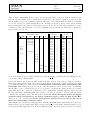
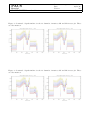
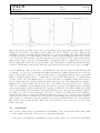
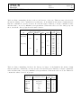
1
PACS
Herschel
FM ILT PhFPU functional tests
Document:
Date:
Version:
SAp-PACS-MS-0652-06
01/12/06
4.0
Page 1
Report on the FM ILT PhFPU functional tests
Marc Sauvage,
with numerous inputs from
Olivier Boulade,
Eric Doumayrou,
Jérôme Martignac,
Thomas Müller,
and Louis Rodriguez
PACS
Herschel
FM ILT PhFPU functional tests
Version
1.0
2.0
2.1
3.0
Date
30/09/06
10/10/06
11/10/06
29/11/06
4.0
01/12/06
Document:
Date:
Version:
SAp-PACS-MS-0652-06
01/12/06
4.0
Page 2
Document Change Record
Changes
Document creation with tests of 24/08/2006
Included the tests of 17/07/2006
Included a discussion on correlated noise in 24/08/2006
Included the tests of 11/10/2006
Corrected various typos
Included the tests of 31/10/2006
Corrected various typos including the mis-numbering of
Section 5’s conclusions as section 6.
PACS
Herschel
FM ILT PhFPU functional tests
Document:
Date:
Version:
SAp-PACS-MS-0652-06
01/12/06
4.0
Page 3
Contents
1 Reference Documents
6
2 Purpose of this document
6
3 The warm functional tests of 17/07/2006
6
3.1
Test description . . . . . . . . . . . . . . . . . . . . . . . . . . . . . . . . . . . . . . . .
6
3.2
Analysis . . . . . . . . . . . . . . . . . . . . . . . . . . . . . . . . . . . . . . . . . . . .
7
3.2.1
Bias commands execution . . . . . . . . . . . . . . . . . . . . . . . . . . . . . .
7
3.2.2
Signal analysis . . . . . . . . . . . . . . . . . . . . . . . . . . . . . . . . . . . .
13
Conclusions . . . . . . . . . . . . . . . . . . . . . . . . . . . . . . . . . . . . . . . . . .
21
3.3
4 The warm functional tests of 24/08/2006
21
4.1
Test description . . . . . . . . . . . . . . . . . . . . . . . . . . . . . . . . . . . . . . . .
21
4.2
Analysis . . . . . . . . . . . . . . . . . . . . . . . . . . . . . . . . . . . . . . . . . . . .
22
4.2.1
Bias commands execution . . . . . . . . . . . . . . . . . . . . . . . . . . . . . .
22
4.2.2
Signal analysis . . . . . . . . . . . . . . . . . . . . . . . . . . . . . . . . . . . .
27
Conclusions . . . . . . . . . . . . . . . . . . . . . . . . . . . . . . . . . . . . . . . . . .
34
4.3
5 The warm functional tests of 11/10/2006
36
5.1
Test Description . . . . . . . . . . . . . . . . . . . . . . . . . . . . . . . . . . . . . . .
36
5.2
Analysis . . . . . . . . . . . . . . . . . . . . . . . . . . . . . . . . . . . . . . . . . . . .
36
5.2.1
Bias commands execution . . . . . . . . . . . . . . . . . . . . . . . . . . . . . .
36
5.2.2
Signal analysis . . . . . . . . . . . . . . . . . . . . . . . . . . . . . . . . . . . .
40
Conclusions . . . . . . . . . . . . . . . . . . . . . . . . . . . . . . . . . . . . . . . . . .
44
5.3
6 The LTU-driven 4 K functional tests of 31/10/2006
48
6.1
Test Description . . . . . . . . . . . . . . . . . . . . . . . . . . . . . . . . . . . . . . .
48
6.2
Analysis . . . . . . . . . . . . . . . . . . . . . . . . . . . . . . . . . . . . . . . . . . . .
48
6.2.1
Bias commands execution . . . . . . . . . . . . . . . . . . . . . . . . . . . . . .
48
6.2.2
Signal Analysis . . . . . . . . . . . . . . . . . . . . . . . . . . . . . . . . . . . .
51
Conclusions . . . . . . . . . . . . . . . . . . . . . . . . . . . . . . . . . . . . . . . . . .
56
6.3
A The test scripts
58
A.1 Test script of 17/07/2006 . . . . . . . . . . . . . . . . . . . . . . . . . . . . . . . . . .
58
A.2 Test script of 24/08/2006 . . . . . . . . . . . . . . . . . . . . . . . . . . . . . . . . . .
60
A.3 Test script of 11/10/2006 . . . . . . . . . . . . . . . . . . . . . . . . . . . . . . . . . .
60
A.4 Test script of 31/10/2006 . . . . . . . . . . . . . . . . . . . . . . . . . . . . . . . . . .
63
PACS
Herschel
FM ILT PhFPU functional tests
Document:
Date:
Version:
SAp-PACS-MS-0652-06
01/12/06
4.0
Page 4
List of Figures
1
17/07/2006 - Time evolution for the most important biases - test #1 . . . . . . . . . .
10
2
17/07/2006 - Time evolution for the second set of biases - test #1 . . . . . . . . . . .
12
3
17/07/2006 - Signal timeline - Matrices 1 and 2 test #1 . . . . . . . . . . . . . . . . .
13
3
17/07/2006 - Signal timeline - Matrices 5 and 6 test #1 . . . . . . . . . . . . . . . . .
14
3
17/07/2006 - Signal timeline - Matrices 1 and 2 test #2 . . . . . . . . . . . . . . . . .
15
3
17/07/2006 - Signal timeline - Matrices 5 and 6 test #2 . . . . . . . . . . . . . . . . .
15
3
17/07/2006 - Signal timeline - Matrix 1 test #3 . . . . . . . . . . . . . . . . . . . . . .
16
3
17/07/2006 - Signal timeline - Matrix 5 test #3 . . . . . . . . . . . . . . . . . . . . . .
16
4
17/07/2006 - VH-VL sequence on matrices M1 and M2 - test #1 . . . . . . . . . . . . .
17
4
17/07/2006 - VH-VL sequence on matrices M5 and M6 - test #1 . . . . . . . . . . . . .
18
4
17/07/2006 - VH-VL sequence on matrices M1 and M2 - test #2 . . . . . . . . . . . . .
19
4
17/07/2006 - VH-VL sequence on matrices M5 and M6 - test #2 . . . . . . . . . . . . .
19
4
17/07/2006 - VH-VL sequence on matrices M1 and M5 - test #3 . . . . . . . . . . . . .
20
5
17/07/2006 - Power spectrum of the signal on M2 during the VH-VL sequence - Test #1 20
6
24/08/2006 - Time evolution for the most important biases - test #1 . . . . . . . . . .
24
7
24/08/2006 - Time evolution for the second set of biases - test #1 . . . . . . . . . . .
25
8
24/08/2006 - Signal timeline - Matrix 1 test #1 . . . . . . . . . . . . . . . . . . . . . .
27
8
24/08/2006 - Signal timeline - Matrix 3 test #1 . . . . . . . . . . . . . . . . . . . . . .
28
8
24/08/2006 - Signal timeline - Matrices 1 and 2 test #2 . . . . . . . . . . . . . . . . .
29
8
24/08/2006 - Signal timeline - Matrices 5 and 6 test #2 . . . . . . . . . . . . . . . . .
29
8
24/08/2006 - Signal timeline - Matrices 1 and 2 test #3 . . . . . . . . . . . . . . . . .
30
8
24/08/2006 - Signal timeline - Matrices 5 and 6 test #3 . . . . . . . . . . . . . . . . .
30
9
24/08/2006 - VH-VL sequence on matrices M1 and M5 - test #1 . . . . . . . . . . . . .
31
9
24/08/2006 - VH-VL sequence on matrices M1 and M2 - test #2 . . . . . . . . . . . . .
32
9
24/08/2006 - VH-VL sequence on matrices M5 and M6 - test #2 . . . . . . . . . . . . .
32
9
24/08/2006 - VH-VL sequence on matrices M1 and M2 - test #3 . . . . . . . . . . . . .
33
9
24/08/2006 - VH-VL sequence on matrices M5 and M6 - test #3 . . . . . . . . . . . . .
33
10
24/08/2006 - Power spectrum of the signal during the VH-VL sequence . . . . . . . . .
34
11
11/10/2006 - Time evolution for the two most important set of biases . . . . . . . . .
38
12
11/10/2006 - Signal timeline - Matrices 1 and 2 . . . . . . . . . . . . . . . . . . . . . .
40
12
11/10/2006 - Signal timeline - matrices 3 and 4 . . . . . . . . . . . . . . . . . . . . . .
41
12
11/10/2006 - Signal timeline - matrices 5 and 6 . . . . . . . . . . . . . . . . . . . . . .
42
12
11/10/2006 - Signal timeline - matrices 7 and 8 . . . . . . . . . . . . . . . . . . . . . .
42
12
11/10/2006 - Signal timeline - matrices 9 and 10 . . . . . . . . . . . . . . . . . . . . .
43
13
11/10/2006 - VH-VL sequence on matrices M1 and M2 . . . . . . . . . . . . . . . . . .
44
13
11/10/2006 - VH-VL sequence on matrices M3 and M4 . . . . . . . . . . . . . . . . . .
45
13
11/10/2006 - VH-VL sequence on matrices M5 and M6 . . . . . . . . . . . . . . . . . .
46
13
11/10/2006 - VH-VL sequence on matrices M7 and M8 . . . . . . . . . . . . . . . . . .
46
PACS
Herschel
FM ILT PhFPU functional tests
Document:
Date:
Version:
SAp-PACS-MS-0652-06
01/12/06
4.0
Page 5
13
11/10/2006 - VH-VL sequence on matrices M9 and M10 . . . . . . . . . . . . . . . . . .
47
14
31/10/2006 - Time evolution for the two most important set of biases . . . . . . . . .
50
15
31/10/2006 - Signal timeline - Matrices 1 and 2 . . . . . . . . . . . . . . . . . . . . . .
53
15
31/10/2006 - Signal timeline - matrices 3 and 4 . . . . . . . . . . . . . . . . . . . . . .
53
15
31/10/2006 - Signal timeline - matrices 5 and 6 . . . . . . . . . . . . . . . . . . . . . .
54
15
31/10/2006 - Signal timeline - matrices 7 and 8 . . . . . . . . . . . . . . . . . . . . . .
54
15
31/10/2006 - Signal timeline - matrices 9 and 10 . . . . . . . . . . . . . . . . . . . . .
55
16
31/10/2006 - Power spectrum of the signal during the VH-VL sequence . . . . . . . . .
57
List of Tables
1
References for the functional tests . . . . . . . . . . . . . . . . . . . . . . . . . . . . .
6
2
17/07/2006 - GND-BU during the tests . . . . . . . . . . . . . . . . . . . . . . . . . . . .
8
3
17/07/2006 - Bias commanding checks for the most important biases - test #1 . . . .
9
4
17/07/2006 - Bias commanding checks for the second bias set - test #1 . . . . . . . .
11
5
17/07/2006 - Bias commanding checks for the last bias set - test #1 . . . . . . . . . .
11
6
24/08/2006 - GND-BU during the tests . . . . . . . . . . . . . . . . . . . . . . . . . . . .
22
7
24/08/2006 - Bias commanding checks for the most important biases - test #1 . . . .
23
8
24/08/2006 - Bias commanding checks for the second bias set - test #1 . . . . . . . .
25
9
24/08/2006 - Bias commanding checks for the last bias set - test #1 . . . . . . . . . .
26
10
11/10/2006 - GND-BU during the tests . . . . . . . . . . . . . . . . . . . . . . . . . . . .
36
11
11/10/2006 - Bias commanding checks for the most important biases . . . . . . . . . .
37
12
11/10/2006 - Bias commanding checks for the second bias set . . . . . . . . . . . . . .
39
13
11/10/2006 - Bias commanding checks for the last bias set . . . . . . . . . . . . . . . .
39
14
31/10/2006 - GND-BU during the tests . . . . . . . . . . . . . . . . . . . . . . . . . . . .
48
15
31/10/2006 - Bias commanding checks for the most important biases . . . . . . . . . .
49
16
31/10/2006 - Bias commanding checks for the second bias set . . . . . . . . . . . . . .
51
17
31/10/2006 - Bias commanding checks for the last bias set . . . . . . . . . . . . . . . .
52
PACS
Herschel
FM ILT PhFPU functional tests
1
SAp-PACS-MS-0652-06
01/12/06
4.0
Page 6
Reference Documents
RD1
RD2
2
Document:
Date:
Version:
SAp-PACS-MS-0616-06
SAp-PACS-MS-0247-04
PACS FM Photometer Focal Plane Unit User’s Manual
PACS CQM Photometer Focal Plane Unit User’s Manual
Purpose of this document
As a series of roughly identical functional tests of the PhFPU will be performed through the course
of the FM ILT, it is probably a good idea to hold in a single document all the results and analyses of
these tests. Part, or the totality of this document will also find its place in the final PACS FM test
report.
Table 1 identifies the different tests analyzed in this report by their date of occurence. For those tests
performed with the PACS warm electronics, the reference of the telemetry filename is also given. The
temperature level at which the tests were performed is indicated. The status column indicates the
processing status for the test data, and “OK” is the label of successful functional tests.
Table 1: References for the functional test. In the status column I give some indication of the
test results. “OK” is for successful tests. “Commanding” implies some inconsistencies between the
commanded biases and the housekeepings, “Signal” means the signal behavior is not what we expect,
and “Noise” means the noise behavior is not what we expect. In all these cases, more details can be
found in the respective sections of this report.
Test Date
17/07/2006
Electronics set-up
LTU+BOLC QM1
Temperature
Warm
filename
private telemetry format
24/08/2006
LTU+BOLC QM1
Warm
private telemetry format
11/10/2006
31/10/2006
LTU+BOLC FM
LTU+BOLC FM
Warm
4K
private telemetry format
private telemetry format
Status
Commanding,
Signal, Noise
Commanding,
Signal, Noise
OK
OK
The rest of this document is a test-by-test report on each functional test. As the purpose of the test
is to first check that the instrument is functional and second to check that it has remained unchanged
since the last occurence of the test, it is impossible to avoid a certain feeling of “déjà vu” (all over
again, as our english-speaking friends would add for some obscure reason) while reading the report.
3
3.1
The warm functional tests of 17/07/2006
Test description
These tests were performed at the end of the integration at Keyser-Threde. The instrument was
warm, and though the PhFPU was in its FM version, a QM version of the warm electronics was used,
namely BOLC QM1. This BOLC version commands only two groups (see RD1 for a description of
the PhFPU warm electronics). Because of this the test script is repeated three times, and each time
the harnesses between BOLC and the PhFPU are moved so that all 6 groups of the PhFPU can be
explored. Because of BOLC QM1, the test script used is different from that described in RD1. The
VH BLIND levels were lower to avoid saturation on BOLC QM1 and no group-per-group VRL scales
PACS
Herschel
FM ILT PhFPU functional tests
Document:
Date:
Version:
SAp-PACS-MS-0652-06
01/12/06
4.0
Page 7
were performed as this made little sense when only two groups could be tested at a time. Finally
one has to remember that because BOLC QM1 can only control two groups, one has to change the
wiring between BOLC and the PhFPU to change the groups that are switched on, but as far as BOLC
is concerned, no change has occured. Therefore in all the tests, we always see the same two groups
switched on (#1 and #3) and we always get data at the same location of the telemetry.
The actual execution of the test that day was the following:
• The first test has BOLC connected to matrices M1, M2, M3 and M4 (i.e. the actual groups 1
and 2). This is test #1 of this section. Telemetry files for this test have a date between 19:33:56
and 19:35:38.
• The harnesses are reconnected so as to now see matrices M5, M6, M7, and M8 (i.e. the actual
groups 3 and 4). Remember that M8 is the matrix with a missing readout channel. This
is test #2 of this section. Telemetry files for this test have a date between 19:48:07 and
19:49:49.
• The harnesses are reconnected so as to now see matrices M9 and M10, the read matrices (i.e.
groups 5 and 6). This is test #3 of this section. Telemetry files for this test have a date between
20:01:48 and 20:03:30.
Before moving on to the analysis, I simply recall that judging from the logbook notes of that test,
everything appeared to proceed correctly.
3.2
Analysis
Because the test was performed with a private equipment, it was also analyzed with a private system,
called PIRE, which is inherited from the CAM interactive analysis and thus is in IDL. An important
aspect is the conversion of the HK information from decimal to analog values. As the test was performed with BOLC QM1, I have used a conversion file called Tm hk QM1.txt. Usinq QM1 conversion
factors actually required some slight modifications of PIRE to make it more flexible in its handling of
the multiple BOLC versions1 .
The analysis performed is rather straightforward: first we inspect the biases time sequence to check
that the bias commands are correctly executed, then we turn to the pixel signal to check that we
observe the expected variations.
3.2.1
Bias commands execution
The first step here is to check the value of GND-BU as this value will be present in all the BU HKs
and thus we need to add it to all the BU commands to check whether the command matches the HK.
Remember that this bias is either on or off, i.e. one does not command its value, it has to be read in
the HK themselves, and there is one value per group. In the current test GND-BU is around 0.46 V (see
table 2 for the actual median value of GND-BU). Note that the rms of GND-BU during a test is typically
around 1-2 mV.
There are a large number of biases that can be set in each group, but for the purpose of this test, we
can restrict our inspection to the biases that see their state change during the test. This give a total
of 18 biases that I have grouped into 3 sets. The first set contains the biases that, at some point in
1
As of 03/10/06, these have now been integrated in the reference version of PIRE.
PACS
Herschel
FM ILT PhFPU functional tests
Document:
Date:
Version:
SAp-PACS-MS-0652-06
01/12/06
4.0
Page 8
Table 2: The value of GND-BU measured during the three tests. The units are Volts
Test #1
Group 1 Group 3
0.463
0.462
17/07/2006
Test #1
Group 1 Group 3
0.463
0.462
Test #1
Group 1 Group 3
0.463
0.463
the test, generate the signal changes, the second set contains the biases that need to be modified so
that the signal changes are visible, and the last set contains similar biases but that are commanded
only once during the test. I do not show here the biases that are never commended (and hence set
at 0 V by the reset all bias command at the start of the test procedure) or commanded to be at
0 V during the script. In fact only two biases are in that category: VCH and VSMS-H. I have however
checked that they are indeed at 0 V during the whole test.
The first set of biases contains VH BLIND, VDD, VRL, VH, and VL. Remember that VDD is a BU bias hence
the comparison between the HK and commanded value has to take into account GND-BU. The time
sequence of commands to these biases, as well as the corresponding HK values, is given in table 3 as
well as displayed graphically on figure 1. There is not significant differences in the housekeeping data
for this set of biases between the three tests, therefore only the data for test #1 are displayed.
As can be seen from table 3 and figure 1, the test appears to proceed quite correctly. Everything
is nominal on group 3, while VDD does not reach the commanded values on group 1, sometimes by
40 mV. We will come back to that later (I have considered that differences between the commanded
and HK value of less than 20 mV are no cause for alarm).
The second set of biases contains VGG, VDECX-H, VDECX-L, CKRLL, CKRLH. Remember that VGG is a BU
bias. Table 4 gives the timeline of the commands to these biases as well as the value read in the HK.
This timeline is graphically displayed on figure 2.
This time the discrepancies are minor and affect only VGG a BU bias, on group 1 again. Interestingly,
VGG is not incorrect when it is set to 0 V, we will come back to that later.
The final set of biases contains those that are set only once, i.e. VGL-BU, VDL-BU, VSS-BU, VGL, VDL,
VSS, VSMS-L, VINJ. For those biases I list in table 5 their commanded values and the measured HK
values. For this set, it is rather straightforward to indentify the BU biases. Note that this is not a
time-ordered table. As with the first two sets of biases, the differences in the HK between the three
tests are not significant.
Here again, there are some discrepant values (mostly for group 1).
In conclusion of this exploration of the bias commanding during the test, we see that almost all of
the biases reach their correct commanded value. However out of the total of 82 commanded
biases, we have 5 major discrepancies (by 40 mV or more) and 7 minor ones (by 20 mV
or more). All these discrepancies occur on group 1.
The first explanation that comes to mind is that this is related to the use of the “all groups” commanding method in the test script. As this uses average conversion factors, this will necessarily lead
to errors at the individual group level. However these errors are too small to explain what we see
here.
Another possibility is that something is wrong either in the analog to digital conversion of the commands or in the digital to analog conversion of the housekeepings. Regarding the digital to analog
conversion of the HK I have tried using the FM conversion coefficients but this did not solve the
PACS
Herschel
FM ILT PhFPU functional tests
Document:
Date:
Version:
SAp-PACS-MS-0652-06
01/12/06
4.0
Page 9
Table 3: Bias commanding checks for the 5 most important biases of the test. This is a time-ordered
table though the timing of the commands is not indicated. The status column is decided upon the
match quality between the commanded and the HK value. A checkmark indicates that the command
is correctly executed, a question mark that some discussion is required, and a double question mark
that an investigation is required. Units in the table are Volts. For the BU biases, I indicate both the
commanded value and that value corrected by GND-BU level in parenthesis. This table contains the
time sequence for test #1.
VH BLIND
0.70
0.72
0.74
0.76
1.30
1.10
17/07/2006
Group 1
Bias setting values
VDD
VRL
VH
VL
Value Status
√
0.69
1.64
?
1.20 (1.66)
1.22 (1.68)
1.66
?
1.24 (1.70)
1.68
?
1.26 (1.72)
1.70
?
√
0.71
√
0.73
√
0.75
2.60 (3.06)
3.02
??
√
1.29
√
0.30
0.31
√
0.40
0.41
√
0.50
0.51
√
0.40
0.41
√
0.30
0.30
√
1.09
√
0.10
0.10
√
−0.1 −0.10
√
0.00
0.00
√
0.00
0.00
Group 3
Value Status
√
0.70
√
1.66
√
1.68
√
1.70
√
1.72
√
0.72
√
0.74
√
0.76
√
3.06
√
1.30
√
0.30
√
0.40
√
0.50
√
0.40
√
0.30
√
1.10
√
0.10
√
−0.10
√
0.00
√
0.00
problem. I cannot however exclude that the file called Tm hk QM1.txt that resides in PIRE is not the
correct file to use for BOLC QM1.
On the other hand, since I have the LTU logfile I can make a check of the analog to digital conversion.
First, I have inspected the logfile and converted again almost all the analog values to their hexadecimal
codes using the FM tables. This reveals that almost all the conversions where indeed done with
FM tables. This is likely the reason for most of the discrepancies observed between the commanding
and the HK, i.e. the conversion tables do not correspond to the hardware. This can indeed be verified
using RD2 where the conversion coefficients for the commanding of BOLC QM1 are listed. For all
the biases showing commanding/HK descrepancies of tables 7 to 9 I have converted back the digital
command into an analog value. This shows indeed that for all the discrepant biases, the digital
command used corresponds to an analog command equal to what we find in the HK.
Therefore we can conclude that all the discrepancies observed here are due to the use of
incorrect commanding conversion tables.
This analysis also revealed two intriguing facts: first the VH BLIND hexadecimal values are offset by 3
units from the expected values using FM conversion tables. Second the VGG command setting it to 0 V
as the hexadecimal argument 0001. Both the QM1 and FM conversion tables would give a negative
PACS
Herschel
FM ILT PhFPU functional tests
Document:
Date:
Version:
SAp-PACS-MS-0652-06
01/12/06
4.0
Page 10
Figure 1: Time evolution for the 5 most important biases. Units on this figure are Volts. Note that
to produce a clean figure, I have median-filtered the HK values. On the figure, I give the actual HK
values, uncorrected for the GND-BU level. This figure shows test #1.
code for a command of 0 V so this is in fact a protective feature of the LTU software. This is why for
that command we indeed get what we want (0001 is virtually indistinguishable from 0000, i.e. 0 V on
VGG), while non-0 V commands on VGG reveal the commanding problem.
Document:
Date:
Version:
PACS
Herschel
FM ILT PhFPU functional tests
SAp-PACS-MS-0652-06
01/12/06
4.0
Page 11
Table 4: Bias commanding checks for the second bias set of the test. This is a time-ordered table
though the timing of the commands is not indicated. A checkmark in the status column indicates
that the command is correctly executed. For the BU biases, I indicate both the commanded value and
that value corrected by GND-BU level in parenthesis. Units in the table are Volts. This table contains
the time sequence test #1.
VGG
0.0 (0.46)
1.9 (2.36)
17/07/2006
Bias setting values
VDECX-H VDECX-L CKRLL CKRLH
0.0
0.0
1.5
1.5
1.8 (2.26)
0.0
0.0
2.0
2.0
0.0
2.0
Group 1
Value Status
√
0.46
2.34
?
√
0.00
√
0.00
√
1.51
√
1.51
2.24
?
√
0.00
√
0.00
√
2.01
√
2.01
√
0.00
√
2.01
Group 3
Value Status
√
0.46
√
2.36
√
0.00
√
0.00
√
1.50
√
1.50
√
2.26
√
0.00
√
0.00
√
2.00
√
2.00
√
0.00
√
2.00
Table 5: Bias commanding checks for the last set for biases. A checkmark in the status column
indicates that the command is correctly executed. For the BU biases, I indicate both the commanded
value and that value corrected by GND-BU level in parenthesis. Units in the table are Volts. This table
contains the values observed during test #1
Bias name
VGL-BU
VDL-BU
VSS-BU
VGL
VDL
VSS
VSMS-L
VINJ
17/07/2006
Commanded values
Group 1
Value Status
3.0 (3.46)
3.42
??
4.2 (4.66)
4.60
??
√
1.0 (1.46)
1.45
3.0
3.02
?
3.04
??
3.0
√
0.7
0.70
√
3.0
3.01
3.0
3.04
??
Group 3
Value Status
√
3.46
√
4.65
√
1.46
√
3.00
√
3.00
√
0.70
√
3.00
√
3.00
PACS
Herschel
FM ILT PhFPU functional tests
Document:
Date:
Version:
SAp-PACS-MS-0652-06
01/12/06
4.0
Page 12
Figure 2: Time evolution for the second set of biases. Units on this figure are Volts. Note that to
produce a clean figure, I have median-filtered the HK values. On the figure, I give the actual HK
values, uncorrected for the GND-BU level. This figure shows test #1.
PACS
Herschel
FM ILT PhFPU functional tests
3.2.2
Document:
Date:
Version:
SAp-PACS-MS-0652-06
01/12/06
4.0
Page 13
Signal analysis
We now turn to the data part of the telemetry. As explained in the test description, we expect to
have in test #1 and #2 data at the telemetry location of M1, M2, M5 and M6, while for test #3 we
expect to have data only at the telemetry location of M1 and M5. This is indeed the case and thus it
is a relief2 .
The complete sequence: The analysis of the signal is straightforward. Since the signal is completely generated by the bias commands (i.e. none is due to the sensitive part of the bolometer),
we only need to check one pixel per readout channel, i.e. 16 pixels per matrix. Because PIRE is
a homemade IDL package, it is not completely straightforward to know which index of the arrays
corresponds to the channel. To circumvent this, I have extracted the signal on pixels (i, i), with i from
0 to 15. I plot the timeline of each of these pixels and compare it to the reference one shown in RD1.
All these timelines (160 in total) are shown in figure 3.
Figure 3: Signal timeline for the 16 channels of matrices M1 and M2 in test #1. These are two blue
matrices. Note that each timeline is artificially offset from the previous one for clarity. The first 4
downward steps correspond to the VDD sequence. The following 3 upward steps correspond to the
VH BLIND scale. They are followed by another upward step corresponding to the setting of VH BLIND
before the VRL scale. This VRL scale is the symetric 5-steps sequence. Then we have a long plateau that
corresponds to the VH-VL sequence, invisible with this dynamical range (but see figure 4), followed
by the sequence of readout modes Sbolo only, Sref only and Sbolo−Sref. For this last sequence
we observe a clear difference with the reference sequence of RD1: the signal in the Sbolo only is
higher that in Sref only here while the opposite is true in RD1. See the text for a discussion of this
discrepancy.
Each of the channels displayed on figure 3 except one3 shows a similar pattern, which is a first good
sign. This pattern is almost identical to that of RD1: the first 4 downward steps correspond to the
VDD sequence. The following 3 upward steps correspond to the VH BLIND scale. They are followed by
another upward step corresponding to the setting of VH BLIND before the VRL scale. This VRL scale is
the symetric 5-steps sequence. Then we have a long plateau that corresponds to the VH-VL sequence,
2
3
Remember also that PIRE is in IDL and thus the index of M1 is 0. . .
This is the absent channel of matrix M8, so this is expected and part of the “success” criteria for the functional test.
PACS
Herschel
FM ILT PhFPU functional tests
Document:
Date:
Version:
SAp-PACS-MS-0652-06
01/12/06
4.0
Page 14
Figure 3: Continued. Signal timeline for the 16 channels of matrices M5 and M6 in test #1. These
are blue matrices.
invisible when the full dynamical range is used (see later), followed by the sequence of readout modes
Sbolo only, Sref only and Sbolo−Sref. It is for this last sequence that we observe a clear
difference with the reference sequence of RD1: the signal in the Sbolo only is higher that in
Sref only here while the opposite is true in RD1.
The reason for this difference is not straightforward: it cannot be the different VH BLIND levels used
for this run, as the VH BLIND differenciation is performed whatever the readout mode (see RD1). It
should therefore not affect the relative positionning of the Sbolo only and Sref only signals. It is
very unlikely that it is a result of the FM/QM1 commanding problem as this affects only group 1
biases yet both group 1 and group 3 signals show the same behavior.
PACS
Herschel
FM ILT PhFPU functional tests
Document:
Date:
Version:
SAp-PACS-MS-0652-06
01/12/06
4.0
Page 15
Figure 3: Continued. Signal timeline for the 16 channels of matrices M1 and M2 in test #2. These
are blue matrices.
Figure 3: Continued. Signal timeline for the 16 channels of matrices M5 and M6 in test #2. These
are blue matrices. In fact, M6 is really M8 of the PhFPU as can be seen from the missing channel.
PACS
Herschel
FM ILT PhFPU functional tests
Document:
Date:
Version:
SAp-PACS-MS-0652-06
01/12/06
4.0
Page 16
Figure 3: Continued. Signal timeline for the 16 channels of matrix M1 in test #3. This is a red
matrix.
Figure 3: Continued. Signal timeline for the 16 channels of matrix M5 in test #3. This is a red
matrix.
PACS
Herschel
FM ILT PhFPU functional tests
Document:
Date:
Version:
SAp-PACS-MS-0652-06
01/12/06
4.0
Page 17
The VH-VL sequence: When the instrument is warm, it is extremely hard to see the effect of the
VH-VL sequence (see appendix A) when the full dynamical range is used. It is in fact also hard to
clearly identify on a pixel level (VH and VL are used to adjust the value of the mid-point voltage, but
when the system is warm this is very inefficient). Thus I have instead build the average signal per
matrix and this is what is displayed on figure 4, with the value of VH and VL superimposed.
Figure 4: The VH-VL sequence as observed on the mean signal for matrices M1 and M2 during test #1.
These are blue matrices. The effect of changing these biases is evident on the mean signal, while it is
much more difficult to indentify at a pixel level. The transitory period that follows any bias change
is most evident at the start of the sequence at this scale. Also evident is the presence of “non-white”
noise on the data, that is clearly correlated between matrices (see text for analysis).
The first important point to stress is that the global behavior of the VH-VL sequence is in accordance
with the expectations. Remember that we are during this part of the test in the mode Sref only,
i.e. that we are reading the bolometer “signal”, or the midpoint bias level and that this signal is
affected by a minus sign4 . Therefore decreasing the midpoint level (by decreasing VH or VL) increases
the signal level. Thus this part of the test sequence is successful. The second point is a little bit
more worrying: during test #1, we observe the presence of a supplementary noise component that
is correlated between matrices of a given group as well as between groups. To try and identify the
origin of this noise component we have computed the power spectrum of the signal during the VH-VL
sequence. This is in fact not a simple task as this sequence is not meant to compute power spectrum,
i.e. the plateaus are rather short (about 200 readouts each), thus the resulting power spectrum is
itself not well sampled. Therefore I had to separate the VH-VL sequence into four parts, corresponding
to the 4 different settings of the (VH,VL) pair. For each sequence I have performed of power spectrum
calculation. Figure 5 shows on of these power spectra, here obtained from the second part of the
VH-VL sequence for (VH,VL) at (0.1, −0.1) on matrix M2 during test #1. This figure nicely shows a
rather typical situation for test #1: the power spectra show a rather strong component at 10 Hz. For
some sequences, the peak is smaller and wider but this is likely due to the small number of samples
(200) used to compute the power spectrum.
This is a situation that has occured before at SAp and corresponds to the pick-up of the general 50 Hz
frequency of the lab’s power supply though various channels that are not (or sometimes cannot be)
completely shielded. This origin can help understand why this noise component is quite correlated
4
Those who are lost now should check back into RD1.
PACS
Herschel
FM ILT PhFPU functional tests
Document:
Date:
Version:
SAp-PACS-MS-0652-06
01/12/06
4.0
Page 18
Figure 4: Continued, this time for matrices M5 and M6 during test #1. As can be seen the “non-white”
noise component is also correlated between groups.
between matrices and groups during a given test. Its physical origin is probably related to the fact
that the test equipment used here does not guarantee a complete shielding of the PhFPU-BOLC
system. The QM harnesses used to connect BOLC QM1 need special adapters to connect to the FM
PhFPU and these break the shielding continuity. When the complete FM instrument is assembled,
the PhFPU and BOLC will be completely shielded.
I have performed the same exercice for test #2, where figure 4 seems to indicate that this noise
component is absent. This reveals that we in fact still pick up the 10 Hz noise component, but at
a much fainter level (the peak’s height is generally a factor 3 to 10 times smaller). If one wants to
be optimistic, this variation in the amplitude of the 10 Hz component can be seen as a confirmation
that it is indeed due to noise pick-up through the BOLC-PhFPU connection harnesses, are these are
disconnected and reconnected between tests.
PACS
Herschel
FM ILT PhFPU functional tests
Document:
Date:
Version:
SAp-PACS-MS-0652-06
01/12/06
4.0
Page 19
Figure 4: Continued, this time for matrices M1 and M2 during test #2. The “non-white” noise
component is not present here so the transitory periods are much more evident.
Figure 4: Continued, this time for matrices M5 and M6 during test #2. The “non-white” noise
component is not present here so the transitory periods are much more evident. The data line shows
quite a lot of spikes that were not present on figure 3. This is because here the signal was not
median-filtered.
PACS
Herschel
FM ILT PhFPU functional tests
Document:
Date:
Version:
SAp-PACS-MS-0652-06
01/12/06
4.0
Page 20
Figure 4: Continued, this time for matrices M1 and M5 during test #3. Contrary to the previous
panels, as these are the two red matrices, the data are obtained from two different groups. The
“non-white” noise component is not present here so the transitory periods are much more evident.
Figure 5: The power spectrum of the mean signal on matrix M2 observed during the second part of
the VH-VL sequence (VH = 0.1, VL = −0.1) V of test #1.
PACS
Herschel
FM ILT PhFPU functional tests
3.3
Document:
Date:
Version:
SAp-PACS-MS-0652-06
01/12/06
4.0
Page 21
Conclusions
The objective of this test is to check that all electrical lines to the bolometers are functionning. This
objective is fully reached here. However it is worth mentioning that:
• One has to check that the commanding conversion tables correspond to the version of the BOLC
hardware used.
• The relative level of the signal between the Sref only and the Sb only mode is different from
that observed in SAp, and the origin of this is unknown.
• We pick up an extra noise component with a characteristic frequency of 10 Hz, which is likely
due to the general lab power supply 50 Hz frequency and the lack of complete shielding between
BOLC QM1 and the FM PhFPU. This shielding will be complete when BOLC FM is used.
• The current procedure is not adequate to quantify the noise on the signal (it was not meant to
be). Since we do observe extra noise sources, it would be good to introduce a “waiting” plateau
after the VH-VL sequence long enough to accumulate more than 200 samples on the signal.
4
The warm functional tests of 24/08/2006
4.1
Test description
These tests were performed at the end of the integration of the PhFPU at MPE. The instrument
was obviously warm and since the FM warm electronics of PACS was not complete, we have used
the SAp Local Test Unit (LTU) to perform the test. Another major difference in the setup is the
use of the QM1 version of BOLC, rather than the FM version. This BOLC model can only control
two groups, therefore a series of tests had to be performed to explore the behavior of all the groups
of the PhFPU (see RD1 for a description of the PhFPU warm electronics). Also, because of BOLC
QM1 peculiarities, some differences exist between the test script as described in RD1, and the actual
test script used here: The VH BLIND levels were lower to avoid saturation on BOLC QM1 and no
group-per-group VRL scales were performed as this made little sense when only two groups could be
tested at a time. Finally one has to remember that because BOLC QM1 can only control two groups,
one has to change the wiring between BOLC and the PhFPU to change the groups that are switched
on, but as far as BOLC is concerned, no change has occured. Therefore in all the tests, we always see
the same two groups switched on (#1 and #3) and we always get data at the same location of the
telemetry.
The actual test execution was as follows:
• A first run was performed with BOLC connected to groups 5 and 6 of the PhFPU, i.e. the two
red matrices (M9 and M10). In this test, stops were placed at crucial points to allow visual
checking of the test progress (mostly the execution of bias commands). This test was performed
mostly to validate the test script in the present electronics configuration and is not analyzed
here.
• This first test was repeated, without the stops. In this section this is going to be test #1.
• The wiring between BOLC and the PhFPU was changed so that BOLC was connected to groups
1 and 2, i.e. matrices M1, M2, M3, and M4, and the test script was repeated. In this section
this is going to be test #2.
PACS
Herschel
FM ILT PhFPU functional tests
Document:
Date:
Version:
SAp-PACS-MS-0652-06
01/12/06
4.0
Page 22
• The wiring between BOLC and the PhFPU was changed again so that BOLC was connected to
groups 3 and 4, i.e. matrices M5, M6, M7, and M8. In this section this is going to be test #3.
Telemetry recording was started each time after the sequencer loading script, but with a variable delay
before the start of the actual test scripts, therefore tests #1, #2 and #3 differ slightly in their initial
sequence.
4.2
Analysis
Similarly to the 17/07/06 tests, these were analyzed with PIRE, with the conversion file called
Tm hk QM1.txt to transform the HK into analog values.
The analysis performed is rather straightforward: first we inspect the biases time sequence to check
that the bias commands are correctly executed, then we turn to the pixel signal to check that we
observe the expected variations.
4.2.1
Bias commands execution
When performing this part of the analysis, remember that for all the BU biases one has to add the
value of GND-BU to all the commanded values before comparing them to the HK values. In the current
test, GND-BU is around 0.46 V (see table 6 for the actual median value of GND-BU). As can be seen from
a comparison with table 2, changes of the order of 1 mV have occured. This is not significant.
Table 6: The median value of GND-BU measured during the three tests. The units are Volts
Test #1
Group 1 Group 3
0.463
0.463
24/08/2006
Test #2
Group 1 Group 3
0.463
0.462
Test #3
Group 1 Group 3
0.462
0.462
For the sake of clarity, I have grouped the biases in three sets.
The first set contains the biases that are extensively used in the test, either because we regularly need
to tune the electronics with them or because we rely on these biases in the test. This group contains
VH BLIND, VDD, VRL, VH, and VL. Table 7 lists the time sequence of the commands to these biases as well
as the status of the command deduced from the HK. Figure 6 shows graphically the time evolution
of these biases. For this part of the test analysis, it turns out that the differences between the three
tests are very small, so I have only displayed the information for test #1.
At this point, It appears that the test is proceeding nominally, apart from differences between the
commanded and housekeeping values for group 1 (on VDD essentially). Interestingly, at the 10 mV
accuracy, we observe no difference in the bias setting between this test and that of 17/07/06. Given
that the test script is exactly the same, this is both expected and welcome.
In the second set of biases, I have placed biases which are set more than once during the script
although they are not directly responsible for the signal variation in the test. They are adjusted so
that we can see the signal variation. These biases are VGG, VDECX-H, VDECX-L, CKRLL and CKRLH. As
for the first set of bias, I have placed in table 8 the time-ordered sequence of bias setting commands
and their execution status. Figure 7 shows the graphical timeline of these biases. Since most of them
have the same values, I have introduced artificial offsets so that the figure becomes clearer. Here again
PACS
Herschel
FM ILT PhFPU functional tests
Document:
Date:
Version:
SAp-PACS-MS-0652-06
01/12/06
4.0
Page 23
Table 7: Bias commanding checks for the 5 most important biases of the test. This is a time-ordered
table though the timing of the commands is not indicated. A checkmark in the status column indicates
that the command is correctly executed, a question mark that some discussion is required, and a double
question mark that an investigation is required. Units in the table are Volts. For the BU biases, I
indicate both the commanded value and that value corrected by GND-BU level in parenthesis. This
table contains the time sequence for test #1.
VH BLIND
0.70
0.72
0.74
0.76
1.30
1.10
24/08/2006
Bias setting values
Group 1
VDD
VRL
VH
VL
Value Status
√
0.69
1.20 (1.66)
1.64
?
1.22 (1.68)
1.66
?
1.24 (1.70)
1.68
?
1.26 (1.72)
1.70
?
√
0.71
√
0.73
√
0.75
3.02
??
2.60 (3.06)
√
1.29
√
0.30
0.31
√
0.40
0.41
√
0.50
0.51
√
0.40
0.41
√
0.30
0.30
√
1.09
√
0.10
0.10
√
−0.1 −0.10
√
0.00
0.00
√
0.00
0.00
Group 3
Value Status
√
0.70
√
1.66
√
1.68
√
1.70
√
1.72
√
0.72
√
0.74
√
0.76
√
3.06
√
1.30
√
0.30
√
0.40
√
0.50
√
0.40
√
0.30
√
1.10
√
0.10
√
−0.10
√
0.00
√
0.00
the differences observed between the three tests are extremely small and for clarity I have only shown
the information related to test #1.
For this second set of bias we observe again that the test appears to proceed quite nominally, except
for some slightly discrepant values on VGG for group 1, Again a situation identical as that observed on
17/07/06.
Thirdly there is a last set of biases that I’ve grouped together because they are only set once (I do
not include biases that are set to 0 V. Those are commanded with the 0000 hexadecimal code which
is always correct). This last set contains VGL-BU, VDL-BU, VSS-BU, VGL, VDL, VSS, VSMS-L, and VINJ.
Table 9 compares the commanded values for these biases to the observed value. This table is not timeordered as those biases are only set once during the test. Again no significant difference is observed
between the three tests so only the information of test #1 is given.
Here again, there are some slightly discrepant values (mostly for group 1), exactly identical to those
we found during the tests of 17/07/2006.
Finally the two remaining biases VCH, and VSMS-H that are supposed to remain at 0 V. I have checked
that this is indeed the case during all three tests.
In conclusion of this exploration of the bias commanding during this test, we see that we are exactly in
PACS
Herschel
FM ILT PhFPU functional tests
Document:
Date:
Version:
SAp-PACS-MS-0652-06
01/12/06
4.0
Page 24
Figure 6: Time evolution for the 5 most important biases. Units on this figure are Volts. Note that
to produce a clean figure, I have median-filtered the HK values. On the figure, I give the actual HK
values, uncorrected for the GND-BU level. This figure shows test #1.
the same situation as on 17/07/2006. Therefore we know that the reason for the bias command/HK
discrepancies is the use of incorrect commanding tables. One should remark that the purpose of
repeating these tests is to make sure nothing changes between each occurence of the test. As far as
the biases are concerned, this is indeed the case and thus the test is successful.
Document:
Date:
Version:
PACS
Herschel
FM ILT PhFPU functional tests
SAp-PACS-MS-0652-06
01/12/06
4.0
Page 25
Table 8: Bias commanding checks for the second bias set of the test. This is a time-ordered table
though the timing of the commands is not indicated. A checkmark in the status column indicates
that the command is correctly executed. For the BU biases, I indicate both the commanded value and
that value corrected by GND-BU level in parenthesis. Units in the table are Volts. This table contains
the time sequence test #1.
VGG
0.0 (0.46)
1.9 (2.36)
24/08/2006
Bias setting values
VDECX-H VDECX-L CKRLL CKRLH
0.0
0.0
1.5
1.5
1.8 (2.26)
0.0
0.0
2.0
2.0
0.0
2.0
Group 1
Value Status
√
0.46
2.34
?
√
0.00
√
0.00
√
1.51
√
1.51
2.24
?
√
0.00
√
0.00
√
2.01
√
2.01
√
0.00
√
2.01
Group 3
Value Status
√
0.46
√
2.36
√
0.00
√
0.00
√
1.50
√
1.50
√
2.26
√
0.00
√
0.00
√
2.00
√
2.00
√
0.00
√
2.00
Figure 7: Time evolution for the second set of biases. Units on this figure are Volts. Note that to
produce a clean figure, I have median-filtered the HK values. On the figure, I give the actual HK
values, uncorrected for the GND-BU level. This figure shows test #1.
PACS
Herschel
FM ILT PhFPU functional tests
Document:
Date:
Version:
SAp-PACS-MS-0652-06
01/12/06
4.0
Page 26
Table 9: Bias commanding checks for the last set for biases. A checkmark in the status column
indicates that the command is correctly executed. For the BU biases, I indicate both the commanded
value and that value corrected by GND-BU level in parenthesis. Units in the table are Volts. This table
contains the values observed during test #1
Bias name
VGL-BU
VDL-BU
VSS-BU
VGL
VDL
VSS
VSMS-L
VINJ
24/08/2006
Commanded values
Group 1
Value Status
3.0 (3.46)
3.42
??
4.2 (4.66)
4.60
??
√
1.0 (1.46)
1.45
3.0
3.02
?
3.0
3.04
??
√
0.7
0.70
√
3.0
3.01
3.0
3.04
??
Group 3
Value Status
√
3.46
√
4.65
√
1.46
√
3.00
√
3.00
√
0.70
√
3.00
√
3.00
PACS
Herschel
FM ILT PhFPU functional tests
4.2.2
Document:
Date:
Version:
SAp-PACS-MS-0652-06
01/12/06
4.0
Page 27
Signal analysis
We now turn to the data part of the telemetry. As explained above, because of the hardware configuration, one expects test #1 to have data at the location of M1 and M5, since we are looking at the
red groups, and tests #2 and #3 to have data at the location of M1, M2, M5, M6. This is indeed the
case, and so this is a relief5 .
The complete sequence: the signal analysis is rather straightforward. Since the signal is completely generated by the bias commands (i.e. none of it is due to the sensitive part of the bolometer),
we only need to check one pixel per readout channel, i.e. 16 pixels per matrix. Because PIRE is
a homemade IDL package, it is not completely straightforward to know which index of the arrays
corresponds to the channel. To circumvent this, I have extracted the signal on pixels (i, i), with i from
0 to 15. I plot the timeline of each of these pixels and compare it to the reference one shown in RD1.
All these timelines (160 in total) are shown in figure 8.
Figure 8: Signal timeline for the 16 channels of matrix M1 in test #1. This is one of the red matrix.
Note that each timeline is artificially offset from the previous one for clarity. The first 4 downward
steps correspond to the VDD sequence. The following 3 upward steps correspond to the VH BLIND scale.
They are followed by another upward step corresponding to the setting of VH BLIND before the VRL
scale. This VRL scale is the symetric 5-steps sequence. Then we have a long plateau that corresponds
to the VH-VL sequence, invisible with this dynamical range (but see figure 9), followed by the sequence
of readout modes Sbolo only, Sref only and Sbolo−Sref. For this last sequence we observe a
clear difference with the reference sequence of RD1: the signal in the Sbolo only is higher that in
Sref only here while the opposite is true in RD1. See the text for a discussion of this discrepancy.
Each of the channels displayed on figure 8 except one6 shows a similar pattern, which is a first good
5
6
Remember also that PIRE is in IDL and thus the index of M1 is 0. . .
This is the absent channel of matrix M8, so this is expected and part of the “success” criteria for the functional test.
PACS
Herschel
FM ILT PhFPU functional tests
Document:
Date:
Version:
SAp-PACS-MS-0652-06
01/12/06
4.0
Page 28
Figure 8: Continued. Signal timeline for the 16 channels of matrix M5 in test #1. This is the other
red matrix.
sign. This pattern is almost identical to that of RD1: the first 4 downward steps correspond to the
VDD sequence. The following 3 upward steps correspond to the VH BLIND scale. They are followed by
another upward step corresponding to the setting of VH BLIND before the VRL scale. This VRL scale is
the symetric 5-steps sequence. Then we have a long plateau that corresponds to the VH-VL sequence,
invisible with the full dynamical range (but see later), followed by the sequence of readout modes
Sbolo only, Sref only and Sbolo−Sref. It is for this last sequence that we observe a clear
difference with the reference sequence of RD1: the signal in the Sbolo only is higher that in
Sref only here while the opposite is true in RD1.
The reason for this difference is not straightforward: it cannot be the different VH BLIND levels used
for this run, as the VH BLIND differenciation is performed whatever the readout mode (see RD1). It
should therefore not affect the relative positionning of the Sbolo only and Sref only signals. It is
very unlikely that it is a result of the FM/QM1 commanding problem as this affects only group 1
biases yet both group 1 and group 3 signals show the same behavior.
PACS
Herschel
FM ILT PhFPU functional tests
Document:
Date:
Version:
SAp-PACS-MS-0652-06
01/12/06
4.0
Page 29
Figure 8: Continued. Signal timeline for the 16 channels of matrices M1 and M2 in test #2. These
are blue matrices.
Figure 8: Continued. Signal timeline for the 16 channels of matrices M5 and M6 in test #2. These
are blue matrices.
PACS
Herschel
FM ILT PhFPU functional tests
Document:
Date:
Version:
SAp-PACS-MS-0652-06
01/12/06
4.0
Page 30
Figure 8: Continued. Signal timeline for the 16 channels of matrices M1 and M2 in test #3. These
are blue matrices.
Figure 8: Continued. Signal timeline for the 16 channels of matrices M5 and M6 in test #3. These
are blue matrices. The constant channel on the M6 panel allows the unambiguous identification of
this matrix with matrix M8 of the PhFPU (see RD1).
PACS
Herschel
FM ILT PhFPU functional tests
Document:
Date:
Version:
SAp-PACS-MS-0652-06
01/12/06
4.0
Page 31
The VH-VL sequence: When the instrument is warm, it is extremely hard to see the effect of the
VH-VL sequence (see appendix A) when the full dynamical range is used. It is in fact also hard to
clearly identify on a pixel level (VH and VL are used to adjust the value of the mid-point voltage, but
when the system is warm this is very inefficient). Thus I have instead build the average signal per
matrix and this is what is displayed on figure 9, with the value of VH and VL superimposed.
Figure 9: The VH-VL sequence as observed on the mean signal for matrices M1 and M5 during test #1.
These are red matrices, and contrary to the following figures, they do not belong to the same BOLC
group. The effect of changing the (VH, VL) biases is evident on the mean signal, while it is much
more difficult to indentify at a pixel level. The transitory period that follows any bias change is most
evident at the start of the sequence at this scale. Also evident is the presence of “non-white” noise on
the data, expecially on M5, that is correlated between groups (this will become clearer on the next
panels – see text for analysis).
As with the test of 17/07/2006, the first important point to stress is that the global behavior of the
signal during the VH-VL sequence is as expected. Remember that VH and VL are used to adjust the
level of the midpoint voltage, which is in fact the bolometer signal when the instrument is cold. As
explained in RD1, in readout mode Sref only, which is the mode where we read only the bolometer,
the signal from the bolometer has a minus sign, therefore decreasing the midpoint level (either through
a VH or a a VL decrease) will increase the signal level7 .
But again, as with the test performed on 17/07/2006, we see that we have an extra “non-white” noise
component that is correlated between matrices of the same group and groups of the same test. I
have again performed computations of the power spectra of these mean signals to characterize this
noise source. Each sequence gives rise to 4 spectra as I have to compute one per value of the (VH, VL)
pair. The exploration of the noise properties indicates again that we are picking up the general 50 Hz
modulation from the lab’s power supply, see figure 10. This is not very surprising as the hardware
set-up is the same, i.e. we still suffer from the lack of complete shielding between BOLC QM1 and
the PhFPU. There are two noticeable differences with the tests of 17/07/2006. First the noise level
associated with the 10 Hz component is significantly higher here. I have compared the peak values
observed for each sequence of each matrix during each test and found that on 24/08/2006, they
were 3 to 8 times larger than on 17/07/2006. As the only identified difference lies in the test
7
If you are lost now, it is either a sign that your training in the ways of Saclay’s Fuzzy LogicTM is not complete, or
that you have not read RD1, each being terrible for your karma.
PACS
Herschel
FM ILT PhFPU functional tests
Document:
Date:
Version:
SAp-PACS-MS-0652-06
01/12/06
4.0
Page 32
Figure 9: Continued. The VH-VL sequence as observed on the mean signal for matrices M1 and
M2 during test #2. These are blue matrices, belonging to the same BOLC group. The presence of
“non-white” noise on the data is clearer now, with a strong correlation between matrices of the same
group.
Figure 9: Continued. The VH-VL sequence as observed on the mean signal for matrices M5 and M6
during test #2. These are blue matrices, belonging to the same BOLC group. The “non-white” noise
is indeed correlated between the two active groups of this test.
PACS
Herschel
FM ILT PhFPU functional tests
Document:
Date:
Version:
SAp-PACS-MS-0652-06
01/12/06
4.0
Page 33
Figure 9: Continued. The VH-VL sequence as observed on the mean signal for matrices M1 and M2
during test #3. These are blue matrices, belonging to the same BOLC group.
Figure 9: Continued. The VH-VL sequence as observed on the mean signal for matrices M5 and M6
during test #3. These are blue matrices, belonging to the same BOLC group.
PACS
Herschel
FM ILT PhFPU functional tests
Document:
Date:
Version:
SAp-PACS-MS-0652-06
01/12/06
4.0
Page 34
Figure 10: On the left panel, I show the power spectrum of the mean signal on matrix M2 observed
during the second part of the VH-VL sequence (VH = 0.1, VL = −0.1) V of test #2. This panel is
equivalent to figure 5 and immediately shows that the power in the 10 Hz component is much higher
now (here the peak is 3.5 times higher). This also reveals a frequent situation where the peak has
a lot of structure and its main component appears at a lower frequency. The origin of this effect is
unknown but could be related to the small number of samples we have to compute the power spectra.
On the right panel I show the power spectrum of the mean signal on matrix M1 during the same
sequence, but this time from test #3. Here the peak is strong as well, and better centered at 10 Hz
location (MPE here, KT for the tests of 17/07/2006) we can only hope that the FM shielding will
be efficient. Second we see sometimes the 10 Hz peak shifted to smaller frequencies (as on the left
panel of figure 10) broadened to 2-3 Hz. It is impossible to tell whether this is an effect of the small
number of samples (200) we have to compute the power spectrum. This leads me to recommend that
we place, at the end of the VH-VL sequence, a longer wait time to accumulate frames that would be
used to characterize and possibly identify any mysterious noise source that might affect the signal.
Finally, I have written earlier that the noise due to the 10 Hz component appears very correlated.
This can be quantified. As an example I have used the second part of the VH-VL sequence. Working
on the mean signal per matrix, I find that the correlation coefficient between M2 and M1 is 0.97, that
between M6 and M5 is 0.99, and that between M6 and M1 is 0.96 . Given the hypothesized origin for
the 10 Hz component, it is not surprising to find some correlation, especially on the mean signal per
matrix. However these correlation levels indicate that most of the noise we observe is due to the 10 Hz
component. I have made a small check on the pixel-level signal, using pixel [8,8] in the same sequence.
The correlation coefficients, for the pixel signals, are 0.93 between M2 and M1, 0.98 between M6 and
M5, and 0.97 between M6 and M1. Thus even on the pixel level, most of the noise is due to that
10 Hz component.
4.3
Conclusions
The objective of this test is to check that all electrical lines to the bolometers are functionning. This
objective is fully reached here. However it is worth mentioning that:
• One has to check that the commanding conversion tables correspond to the version of the BOLC
PACS
Herschel
FM ILT PhFPU functional tests
Document:
Date:
Version:
SAp-PACS-MS-0652-06
01/12/06
4.0
Page 35
hardware used.
• The relative level of the signal between the Sref only and the Sb only mode is different from
that observed in SAp, and the origin of this is unknown. This relative position is the same as
that observed in KT on 17/07/2006.
• We pick up an extra noise component with a characteristic frequency of 10 Hz, which is likely
due to the general lab power supply 50 Hz frequency and the lack of complete shielding between
BOLC QM1 and the FM PhFPU. This shielding will be complete when BOLC FM is used,
nevertheless the levels observed at MPE for this component are much higher than those observed
in KT.
• The current procedure is not adequate to quantify the noise on the signal (it was not meant to
be). Since we do observe extra noise sources, it would be good to introduce a “waiting” plateau
after the VH-VL sequence long enough to accumulate more than 200 samples on the signal.
PACS
Herschel
FM ILT PhFPU functional tests
5
Document:
Date:
Version:
SAp-PACS-MS-0652-06
01/12/06
4.0
Page 36
The warm functional tests of 11/10/2006
5.1
Test Description
These tests were performed right at the start of the actual FM ILT. They used the FM version of BOLC
and the SAp Local Test Unit. As such they form the reference against which the tests performed the
following day with the PACS warm electronics and complete FM ILT setup can be compared. This
time we can control the complete instrument (i.e. the 6 groups and the 10 matrices) at once. Since
we have the FM hardware, we are almost back to using the test script described in RD1. Almost only
as we found out that we need to add wait times after the commanding of the protection biases and
GND-BU. This will in fact become the nominal bias setting procedure starting from Draft 7 of RD1.
The actual test execution is much simpler now, and here the complete test script was simply executed
twice. Since the differences between the two run of the test are extremely small, I will not treat them
separately.
5.2
Analysis
Similarly to the previous LTU-operated tests, these tests were analysed with PIRE, in a version that
has been updated to handle correctly the different version of the commanding and HK conversion
tables. We made sure to specify that FM Main versions had to be used here.
The next sections deal with the two steps of the analysis: the bias time sequence and the signal time
signal. In this second section, we pay special attention to the noise characteristics.
5.2.1
Bias commands execution
As usual here we first need to record the values of GNB-BU as this voltage will be added to all the BU
bias values. These values are listed in table 10. They have changed slightly since the previous test
but this can be attributed to the major change that constitutes the replacement of BOLC-QM1 by
BOLC-FM.
Table 10: The median value of GND-BU measured during the LTU tests. The units are Volts. The
values are exactly the same between the two tests, therefore only the values measured during test #1
are shown.
Group 1
0.457
Group 2
0.458
11/10/2006
Group 3 Group 4
0.455
0.457
Group 5
0.459
Group 6
0.459
As usual, to simplify the inspection of the commanding, I group the HK into three sets: those that
are used to modulate the signal during the test, those that are modified so that the signal can be
observed, and those that are set only once.
The comparison between the commanding and the HK for the first set of bias is displayed in table 11
in the time order in which the commanding is made and graphically on the left panel of figure 11. I
only show the values observed on group 1 as all the other groups show identical sequences, once the
marginal difference due to the “all-group” commanding method are taken into account.
Table 11 shows that contrary to what we have observed so far, all biases reach their commanded value
Document:
Date:
Version:
PACS
Herschel
FM ILT PhFPU functional tests
SAp-PACS-MS-0652-06
01/12/06
4.0
Page 37
Table 11: Bias commanding checks for the 5 most important biases of the test. This is a timeordered table though the timing of the commands is not indicated. A checkmark in the status column
indicates that the command is correctly executed. Units in the table are Volts. For the BU biases,
I indicate both the commanded value and that value corrected by GND-BU level in parenthesis. This
table contains the time sequence for group 1. Identical sequences are observed for the other groups,
with marginal differences due to the “all-group” commanding method.
VH BLIND
1.20
11/10/2006
Bias setting values
VDD
VRL
VH
1.20
1.22
1.24
1.26
VL
(1.66)
(1.68)
(1.70)
(1.72)
1.22
1.24
1.26
2.60 (3.06)
1.80
0.30
0.40
0.50
0.40
0.30
1.15
0.10
−0.1
0.00
0.00
Group 1
Value Status
√
1.20
√
1.66
√
1.68
√
1.70
√
1.72
√
1.22
√
1.24
√
1.26
√
3.06
√
1.80
√
0.30
√
0.40
√
0.50
√
0.40
√
0.30
√
1.15
√
0.10
√
−0.10
√
0.00
√
0.00
on all groups. In other terms the commanding system appears to work as long as the right conversion
tables are used.
This impression is confirmed when we turn to the second set of bias, which is again shown as a time
ordered sequence on table 12 and graphically on the right panel of figure 11. As can be seen from the
table, the commands are all perfectly executed.
Finally we examine the last set of bias. Since those are commanded only once, there is no need to
build a timeline and table 13 simply shows the commanded and observed values. This table contains
one question mark, which could ruin the impression given by the previous tables. However inspecting
the biases on the other groups shows that this is an exception. Therefore the conclusion of this
examination of the commanding is that on 11/10/2006, commanding was perfectly executed.
PACS
Herschel
FM ILT PhFPU functional tests
Document:
Date:
Version:
SAp-PACS-MS-0652-06
01/12/06
4.0
Page 38
Figure 11: Left panel: time evolution for the 5 most important biases generating the test signal.
Right panel: time evolution for the second set of biases. Units on this figure are Volts. Note that
to produce a clean figure, I have median-filtered the HK values. On the figure, I give the actual HK
values, uncorrected for the GND-BU level. This figure shows only group 1 data as all the other figures
are identical.
Document:
Date:
Version:
PACS
Herschel
FM ILT PhFPU functional tests
SAp-PACS-MS-0652-06
01/12/06
4.0
Page 39
Table 12: Bias commanding checks for the second bias set of the test. This is a time-ordered table
though the timing of the commands is not indicated. A checkmark in the status column indicates
that the command is correctly executed. For the BU biases, I indicate both the commanded value
and that value corrected by GND-BU level in parenthesis. Units in the table are Volts. Only group 1 is
show, but all the other groups show the same behavior.
VGG
0.0 (0.46)
1.9 (2.36)
11/10/2006
Bias setting values
VDECX-H VDECX-L CKRLL
CKRLH
0.0
0.0
1.5
1.5
1.8 (2.26)
0.0
0.0
2.0
2.0
0.0
2.0
Group 1
Value Status
√
0.46
√
2.36
√
0.00
√
0.00
√
1.50
√
1.50
√
2.26
√
0.00
√
0.00
√
2.00
√
2.00
√
0.00
√
2.00
Table 13: Bias commanding checks for the last set for biases. A checkmark in the status column
indicates that the command is correctly executed. For the BU biases, I indicate both the commanded
value and that value corrected by GND-BU level in parenthesis. Units in the table are Volts. This table
contains the values observed on group 1.
Bias name
VGL-BU
VDL-BU
VSS-BU
VGL
VDL
VSS
VSMS-L
VINJ
11/10/2006
Commanded values
3.0 (3.46)
4.2 (4.66)
1.0 (1.46)
3.0
3.0
0.7
3.0
3.0
Group 1
Value Status
√
3.47
4.68
?
√
1.46
√
3.00
√
3.00
√
0.70
√
3.00
√
3.00
PACS
Herschel
FM ILT PhFPU functional tests
5.2.2
Document:
Date:
Version:
SAp-PACS-MS-0652-06
01/12/06
4.0
Page 40
Signal analysis
Compared to previous test occurences, it will now be much simpler to identify the signals since now
we have everything in its right place (i.e. M1 is at the location of M1, M2 of M2, and so on up to
M10). Therefore I no longer need to specify that they are blue or red.
The complete sequence: Since the signal is completely generated by the bias commands, I only
check pixels (i, i) on each matrix. Thus for each matrix I have 16 timelines that I plot on figure 12,
each displaced by a small amount from the previous one for clarity’s sake. The data are displayed as
raw values as converting them to volts make little sense at this stage.
Figure 12: Signal timeline for the 16 channels of matrices M1 and M2. Note that each timeline is
artificially offset from the previous one for clarity. The first 4 downward steps correspond to the VDD
sequence. The following 3 upward steps correspond to the VH BLIND scale. They are followed by
another upward step corresponding to the setting of VH BLIND before the VRL scale. This VRL scale is
the symetric 5-steps sequence. Then we have a long plateau that corresponds to the VH-VL sequence,
invisible with this dynamical range (but see figure 13), followed by the sequence of readout modes
Sbolo only, Sref only and Sbolo−Sref. For this last sequence we observe now a behavior similar
to the reference sequence of RD1: the signal in Sbolo only is lower that in Sref only. See the text
for a discussion of this return to the normal situation. The data plotted here come from the first run
of the test.
Each of the channels displayed on figure 12 except one8 shows a similar pattern, which is a first good
sign. This pattern is this time identical to that of RD1: the first 4 downward steps correspond to
the VDD sequence. The following 3 upward steps correspond to the VH BLIND scale. They are followed
by another upward step corresponding to the setting of VH BLIND before the VRL scale. This VRL
scale is the symetric 5-steps sequence. Then we have a long plateau that corresponds to the VH-VL
sequence, invisible with the full dynamical range (but see later), followed by the sequence of readout
modes Sbolo only, Sref only and Sbolo−Sref. We now observe the same behaviour as in
8
This is the absent channel of matrix M8, which is observed for the first time at the correct telemetry location since
we can now operate the complete PhFPU with BOLC. Therefore this is really part of the “success” criteria for the
functional test.
PACS
Herschel
FM ILT PhFPU functional tests
Document:
Date:
Version:
SAp-PACS-MS-0652-06
01/12/06
4.0
Page 41
Figure 12: Continued. Signal timeline for the 16 channels of matrices M3 and M4.
the reference sequence of RD1: the signal in the Sbolo only is lower that in Sref only (you
will need to read the PhFPU user’s manual, RD1, to understand why this is compatible with the fact
the the signal in Sbolo−Sref mode is still positive). This is welcome. However we can only conclude
that the relative position of these two modes in terms of signal level is driven by the warm electronics,
and for this we have no good explanation.
PACS
Herschel
FM ILT PhFPU functional tests
Document:
Date:
Version:
SAp-PACS-MS-0652-06
01/12/06
4.0
Page 42
Figure 12: Continued. Signal timeline for the 16 channels of matrices M5 and M6.
Figure 12: Continued. Signal timeline for the 16 channels of matrices M7 and M8.
PACS
Herschel
FM ILT PhFPU functional tests
Document:
Date:
Version:
SAp-PACS-MS-0652-06
01/12/06
4.0
Page 43
Figure 12: Continued. Signal timeline for the 16 channels of matrices M9 and M10.
PACS
Herschel
FM ILT PhFPU functional tests
Document:
Date:
Version:
SAp-PACS-MS-0652-06
01/12/06
4.0
Page 44
The VH-VL sequence Since the instrument is still warm I again examine here the behavior of the
mean signal per matrix during the VH-VL sequence. Figure 13 shows this sequence for each matrix
with the VH and VL sequences superimposed for clarity.
Figure 13: The VH-VL sequence as observed on the mean signal for matrices M1 and M2. The effect of
changing the (VH, VL) biases is evident on the mean signal, while it is much more difficult to indentify
at a pixel level. The transitory period that follows any bias change is most evident at the start of
the sequence at this scale. The “non-white” noise that was apparent in previous test is gone, but the
strong correlations between matrices of a given group is still clear.
This series of figure reveals that the 10 Hz component observed in previous tests is gone. This was
expected since the shielding is much better when the complete FM setup is used, but it is nevertheless
a relief. The power spectrum plots for the VH-VL sequence do not reveal any interesting feature so
I have not displayed them. Similarly to what I had done previously, I have looked at the correlation
coefficients between the mean signals. I again find that there is a very high level of correlation (> 0.9)
between the mean signals of two matrices belonging to the same group (which is not very surprising
given that the signal is completely command-driven), except for group 3, which is principally due
to the high noise level of matrix 6. Now that the 10 Hz component has disappeared, the correlation
coefficient between signals of matrices belonging to different group is compatible with the absence of
correlation. Therefore at this stage we can probably say that in a sequence where the signal is purely
generated by the electronics, there is a strong correlation between signal observed on circuits that have
a large number of components in common (such as within a group), but this correlation disappears
when one compares signals generated through different circuits.
5.3
Conclusions
For this test, all the red lights recorded previously have now turned to green, though we can provide
little explanations for some of these favorable changes:
• Now that the conversion tables are compatible with the test equipment, we find that the agreement between the commanding and the HK values is nominal.
• The relative level of the signal between the Sref only and the Sb only modes is back to what
PACS
Herschel
FM ILT PhFPU functional tests
Document:
Date:
Version:
SAp-PACS-MS-0652-06
01/12/06
4.0
Page 45
Figure 13: Continued. The VH-VL sequence as observed on the mean signal for matrices M3 and M4.
we observed in SAp. This can only mean that this relative positioning is driven by the BOLC
model though we have no explanation for this.
• The extra noise component is gone. This was expected since the shielding of the complete FM
configuration is much better that the shielding for the QM1-FM configuration used previously.
As a result, the correlation, or absence thereof, between different signals is much easier to
understand.
PACS
Herschel
FM ILT PhFPU functional tests
Document:
Date:
Version:
SAp-PACS-MS-0652-06
01/12/06
4.0
Page 46
Figure 13: Continued. The VH-VL sequence as observed on the mean signal for matrices M5 and
M6. In both tests performed that day, the noise level on matrix 6 was significantly higher than that
observed on the other matrices.
Figure 13: Continued. The VH-VL sequence as observed on the mean signal for matrices M7 and M8.
PACS
Herschel
FM ILT PhFPU functional tests
Document:
Date:
Version:
SAp-PACS-MS-0652-06
01/12/06
4.0
Page 47
Figure 13: Continued. The VH-VL sequence as observed on the mean signal for matrices M9 and M10.
PACS
Herschel
FM ILT PhFPU functional tests
6
Document:
Date:
Version:
SAp-PACS-MS-0652-06
01/12/06
4.0
Page 48
The LTU-driven 4 K functional tests of 31/10/2006
In principle, these tests were not supposed to happen. The LTU’s last use should have occured on
October 11, at which point control, and cable connection, was to be surrendered to PACS. However
the repetition of the warm functional test using the PACS FM set-up on October 12 and later on
October 17 revealed mysterious problems (group 6 was on at the start of the October 12 test and
matrix 10, which is on group 6, showed dramatic signal drifts during both tests) that led us to re-open
the LTU box and perform another series of LTU driven tests.
6.1
Test Description
The aim with this series of test was to perform an LTU test that would be as close as possible to the
CUS-driven test, in order to eliminate all possible sources of difference, in case the results observed
with these two set-ups would not be the same. To that effect we introduced artificial delays in the
LTU-driven test. Eventhough we performed more than one test (with or without the delays), I am
only going to present here the results from the last LTU run where the delays are as close as possible
to those introduced by the CUS (if need be, I will refer to this test as the “CUS-like” test). No
execution or signal difference was observed between the different runs. On October 31, this was the 4
fourth test executed. The actual script can be found in Appendix A.
6.2
Analysis
This analysis is done with PIRE, with the same version as that used to analyse the tests of October
11 (PIRE does not evolve much).
6.2.1
Bias commands execution
The first step is to check the values of GND-BU as it is added to all the BU HKs and needs to be
taken into account when checking the correct execution of bias commands. The measured values are
given in table 14. Note that these values are exactly the same as those observed on 11/10/06. This is
supposed to be the case but it nevertheless reassuring.
Table 14: The median value of GND-BU measured during the LTU test. The units are Volts. Only
those values observed during the CUS-like test are shown.
Group 1
0.457
Group 2
0.458
31/10/2006
Group 3 Group 4
0.455
0.457
Group 5
0.459
Group 6
0.459
Let us now turn to the three sets of housekeepings (these three sets are defined as 1: the set of biases
that are used to generate the signal, 2: the set of biases that need to be commanded so that we see the
signal and that are commmanded more than once, and 3: the set of biases that are only commanded
once).
The comparison between the commanded values and the HK for the first set is shown as a timeordered sequence in table 15. Note that since this is a 4 K level test, some of the commanded biases
are different from what we have seen before. Also worth mentionning are the extra VRL steps. These
Document:
Date:
Version:
PACS
Herschel
FM ILT PhFPU functional tests
SAp-PACS-MS-0652-06
01/12/06
4.0
Page 49
come from the fact that we repeat a part of the VRL scale on a group per group basis (rather than on
the usual “all-groups” basis). The bias sequence of this first set is also shown graphically on figure 14.
Here again I will only show in detail what is observed on group 1. No major difference is observed
between groups apart from that due to the “all-groups” commanding scheme.
Table 15: Bias commanding checks for the 5 most important biases of the test. This is a timeordered table though the timing of the commands is not indicated. A checkmark in the status column
indicates that the command is correctly executed. Units in the table are Volts. For the BU biases,
I indicate both the commanded value and that value corrected by GND-BU level in parenthesis. This
table contains the time sequence for group 1. Identical sequences are observed for the other groups,
with marginal differences due to the “all-groups” commanding method. Note that since this is a
4 K-level test the commanded biases are different from those used at 300 K.
VH BLIND
1.50
31/10/2006
Bias setting values
VDD
VRL
VH
1.40
1.42
1.44
1.46
VL
(1.86)
(1.88)
(1.90)
(1.92)
1.52
1.54
1.56
2.60 (3.06)
1.75
0.20
0.30
0.40
0.50
0.20
0.40
0.20
1.70
0.50
−0.15
0.00
0.00
Group 1
Value Status
√
1.50
√
1.86
√
1.88
√
1.80
√
1.82
√
1.52
√
1.54
√
1.56
√
3.06
√
1.75
√
0.20
√
0.30
√
0.40
√
0.30
√
0.20
√
0.40
√
0.20
√
1.70
√
0.50
√
−0.15
√
0.00
√
0.00
Inspection of table 15 reveals that all commands are nominally executed. This is true for all 6 groups
of BOLC. Figure 14 is familiar but nevertheless shows new features that are worth commenting as
this test is in fact the reference LTU-operated 4 K level test.
First, contrary to the test of October 11, we see the setting of almost all biases. This is quite
noticeable on the BU biases that now start with a 0 V value (see for instance VDD). This is due to
three reasons: (1) the command to start downlinking telemetry has been moved to the start of the
script (see Appendix A), (2) because of this shift, we can see the effect of the delays introduced at the
setting of the protection biases and of GND-BU (and that now form the standard procedure to bias the
detectors), and (3) artificial delays are introduced after each command to simulate the fact that with
the flight commanding equipment we cannot send more than two commands per second. Continuing
on the VDD example, after the telemetry is requested, it takes 4 s to switch on GND-BU and another
PACS
Herschel
FM ILT PhFPU functional tests
Document:
Date:
Version:
SAp-PACS-MS-0652-06
01/12/06
4.0
Page 50
Figure 14: Left panel: time evolution for the 5 most important biases generating the test signal. Right
panel: time evolution for the second set of biases. Units on this figure are Volts. On the figure, I
give the actual HK values, uncorrected for the GND-BU level. This, and the fact that we have now
introduced delays between each commands, explains why, for instance, VDD shows an intermediate
level around 0.46 V, which does not appear in table 15. This only signals the switching on of GND-BU
that occurs some time before the commanding of VDD. This figure shows only group 1 data as all the
other figures are identical.
9 s to set VDD to its first commanded value. Previously, all the action before the setting of GNB-BU
was happening before the downlinking of the telemetry, and all commands from the GND-BU setting
to the biasing of VDD proceeded almost instantaneously. Note that the artificial delays could also be
seen with keen eyes and thinner lines as now all of the bias settings occur at different times.
Second, we see a new step on VRL. This corresponds to a repetition of a part of the VRL scale on a
group per group basis. This is why so much time elapses between that repetition on group 1 and the
VH-VL sequence: we need time to repeat the VRL scale on each of the remaining 5 groups successively.
Finally, the values used for the VH-VL sequence are different here.
The second set of bias is explored now. In table 16 we give the time line of bias commands, while this
timeline is also shown graphically on the right panel of figure 14.
Inspection of the housekeepings for the second set of biases (table 16) reveals again that the commanding is nominal. The right panel of figure 14 is also familiar and as the left panel shows the effect
of the artificial commanding delays (see for instance the evolution of VGG: what used to be a very
Document:
Date:
Version:
PACS
Herschel
FM ILT PhFPU functional tests
SAp-PACS-MS-0652-06
01/12/06
4.0
Page 51
Table 16: Bias commanding checks for the second bias set of the test. This is a time-ordered table
though the timing of the commands is not indicated. A checkmark in the status column indicates
that the command is correctly executed. For the BU biases, I indicate both the commanded value and
that value corrected by the GND-BU level in parenthesis. Units in the table are Volts. Only group 1
is show, but all the other groups show the same behavior. Note again some subtle differences in the
commanded bias levels with respect to the 300 K level tests.
VGG
0.00 (0.46)
1.30 (1.76)
31/10/2006
Bias setting values
VDECX-H VDECX-L CKRLL
CKRLH
0.0
0.0
1.5
1.5
1.15 (1.61)
0.0
0.0
2.0
2.0
0.0
2.0
Group 1
Value Status
√
0.46
√
1.76
√
0.00
√
0.00
√
1.50
√
1.50
√
1.61
√
0.00
√
0.00
√
2.00
√
2.00
√
0.00
√
2.00
short spike on the way to its high level is now a minor plateau. Again the purpose of these artificial
delays is to make the LTU-driven test as similar as possible to the CUS-driven test. This way visual
checking of the functional test success is easier and we rule out commanding as a potential source of
problems in the test execution or behavior.
Finally in table 17 we show the measured values of the last set of biases. We find here exactly the
same results as on October 1: all biases are nominally commanded except VDL-BU which is sligthly
discrepant on group 1. This is due to the “all-groups” commanding scheme.
Therefore we conclude that as far as the commanding is concerned, the LTU-operated 4 K level
test of 31/10/2006 was perfectly executed. Let us now turn to the signal recorded during this
test.
6.2.2
Signal Analysis
Just a reminder for those that jump in this document directly here: matrices M1 to M8 are on the
blue array, and matrices M9 and M10 are on the red array.
The complete sequence: If you have RD1 in mind you remember that the readout circuit is
multiplexed, therefore, as we are only checking the electrical continuity of the system here, I only
plot one pixel per channel, i.e. pixels (i, i) on each meatrix. In the figures each timeline is displaced
from the previous one for clarity. The signals are plotted in raw values. First because it does not
really make sense to convert them here, and second because it allows for a check that the three readout
modes (Sbolo only, Sref only and Sbolo−Sref) are correctly understood (the first two are unsigned
16-bits integers with a 0 V level around 16000, and the last one is in signed 16-bits integers with a 0 V
Document:
Date:
Version:
PACS
Herschel
FM ILT PhFPU functional tests
SAp-PACS-MS-0652-06
01/12/06
4.0
Page 52
Table 17: Bias commanding checks for the last set of biases. A checkmark in the status column
indicates that the command is correctly executed. For the BU biases, I indicate both the commanded
value and that value corrected by the GND-BU level in parenthesis. Units in the table are Volts. This
table contains the values observed on group 1 but all the other groups show the same behavior except
for VDL-BU which is only slightly discrepant for group 1.
Bias name
VGL-BU
VDL-BU
VSS-BU
VGL
VDL
VSS
VSMS-L
VINJ
31/10/2006
Commanded values
2.6 (3.06)
4.2 (4.66)
1.5 (1.96)
3.0
3.0
1.3
3.0
3.0
Group 1
Value Status
√
3.06
4.68
?
√
1.95
√
3.00
√
3.00
√
1.30
√
3.00
√
3.00
level at 0). Figure 15 shows the 16 independant channels for each of the 10 matrices.
Since we are now looking for the first time at a test performed at 4 K and given that we have introduced
some differences with respect to the test described in RD1, it is worth spending some time describing
the signal patterns we observe.
Before the test begins, we have a short period of time with no data followed by a strong peak in
the signal that indicates the switch on and biasing of the detectors. The first 4 downward steps that
follow correspond to the VDD sequence. This is known to show a strong relaxation pattern that is very
visible at 4 K. The following 3 upward steps correspond to the VH BLIND scale. These are always much
cleaner as we observe. In this “CUS-like” test, these two sequences are followed by a complex event
corresponding to the preparation of the VRL scale that ends up with the setting of VH BLIND before the
VRL scale. This complex event is simply due to the introduction of artificial delays between each bias
setting. At this location of the test we have 13 biases to set so it takes some time. In previous test
this event was “condensed” in a single spike. The VRL scale is the symetric 5-steps sequence. Then
we have a long plateau during which the group-per-group VRL scale occurs. This plateau ends with
another complex event that signals the preparation of the VH-VL sequence (6 biases to set). This 4
steps VH-VL sequence follows, now clearly visible since we are at 4 K, and the test ends by the sequence
of readout modes Sbolo only, Sref only and Sbolo−Sref.
Taking into account the differences between the test script used here and that of RD1, we can state
that the signal behaves exactly as expected. Therefore regarding the signal behavior, the functional
test of 31/10/06 is a success. With respect to the CUS-driven test that occured in the meantime,
it is worth mentioning that we do not see here the very strong drifts that affected matrix
10 at 300 K. We have no good explanation for this.
PACS
Herschel
FM ILT PhFPU functional tests
Document:
Date:
Version:
SAp-PACS-MS-0652-06
01/12/06
4.0
Page 53
Figure 15: Signal timeline for the 16 channels of matrices M1 and M2. Note that each timeline is
artificially offset from the previous one for clarity. The first 4 downward steps correspond to the VDD
sequence. The following 3 upward steps correspond to the VH BLIND scale. In this “CUS-like” test,
they are followed by a complex event corresponding to the preparation of the VRL scale that ends up
with the setting of VH BLIND before the VRL scale. This VRL scale is the symetric 5-steps sequence.
Then we have a long plateau during which the group-per-group VRL scale occurs. This plateau ends
with a rather complex event that signals the preparation of the VH-VL sequence. This 4 steps VH-VL
sequence follows, now clearly visible since we are at 4 K, and the test ends by the sequence of readout
modes Sbolo only, Sref only and Sbolo−Sref. We observe a behavior similar to the reference
sequence of RD1: the signal in Sbolo only is lower that in Sref only.
Figure 15: Continued. Signal timeline for the 16 channels of matrices M3 and M4.
PACS
Herschel
FM ILT PhFPU functional tests
Document:
Date:
Version:
SAp-PACS-MS-0652-06
01/12/06
4.0
Page 54
Figure 15: Continued. Signal timeline for the 16 channels of matrices M5 and M6.
Figure 15: Continued. Signal timeline for the 16 channels of matrices M7 and M8.
PACS
Herschel
FM ILT PhFPU functional tests
Document:
Date:
Version:
SAp-PACS-MS-0652-06
01/12/06
4.0
Page 55
Figure 15: Continued. Signal timeline for the 16 channels of matrices M9 and M10.
PACS
Herschel
FM ILT PhFPU functional tests
Document:
Date:
Version:
SAp-PACS-MS-0652-06
01/12/06
4.0
Page 56
The VH-VL sequence: In previous, warm, tests I needed to devote a section to this sequence as it
was invisible on the pixel signal and I had to use the mean signal per matrix. This is no longer needed
here in principle as the sequence is fully visible on figure 15. It is even more so in the mean signal
that is so clean that it looks artificial.
Noise properties:
In previous tests I have used the VH-VL sequence to comment on the noise
properties of each matrix and correlation coefficients between the different matrices. As this still has
some interest, I shall explore this now. Rather than using the mean of the full matrix, which is too
clean a signal, it shall use the mean of the central 4×4 pixels area. Because the changes of VH and
VL create such drastic changes of the signal level, a fourier analysis of the noise has to be restricted
to a constant (VH, VL) set. I have chosen the section where VH is 0 V and VL is −0.15 V, because it
is far away from the start of the sequence while still creating a polarization on the bolometer bridge.
This is important because the start of the sequence creates a strong transient effect that is seen on
all arrays. Finally when doing this analysis, one has to remember that the gain is set to high at the
start of the sequence (while it was low for the rest of the test). This means with BOLC FM a gain of
5 µV/ADU
The noise power spectrum is very clean, as figure 16 shows. We have no spurious spike in the spectrum.
However we see two things. First we still have a rather strong component at low frequency. This is
due to the transient effect on the signal. Second the noise level is different from what we had at 300 K.
It is now around 1-2 10−5 V.Hz−1/2 . This is quite higher than what we observed at 300 K. But this is
not a real problem: at 300 K we were not picking up noise from the bolometer bridge, but rather from
the electronics. At 4 K the bolometer bridge starts to be reactive, as revealed by the fact that we see
dead pixels at that temperature. Hence we are starting to pick up its contribution to the noise. Since
we are far from the operating conditions the fact that it is quite high is no cause for alarm. Finally
on the noise issue, matrix 6 is no longer noisier that the other matrices.
Regarding the correlation between signals observed on different matrices, I first measure that all signals
are strongly correlated (correlation coefficients of 0.65 and greater) whatever the pair of matrices used.
However this is strictly due to the strong transient that affect all matrices. If I subtract from each
signal its median filtered version (using a large median window, e.g. 21 readouts) I see that the
resulting signals are completely uncorrelated, even for two matrices of the same group
6.3
Conclusions
Inspection of this test show that is was performed successfully, be it from the commanding side or
from the signal side. We can therefore consider that it constitutes the reference LTU-driven 4 K level
test, and that the LTU can now be safely put back in its box.
The explanation for the strong drifts observed with the CUS-driven 300 K level test has however not
been found.
PACS
Herschel
FM ILT PhFPU functional tests
Document:
Date:
Version:
SAp-PACS-MS-0652-06
01/12/06
4.0
Page 57
Figure 16: The power spectrum of the mean signal on the central 4×4 pixels area of matrix M6
observed during the third part of the VH-VL sequence (VH = 0.0, VL = −0.15) V of test #4. We
see a strong low-frequency component corresponding to the long-term transient seen in the signal.
Otherwise the noise level is quite homogenous, although higher than observed during the 300 K tests.
PACS
Herschel
FM ILT PhFPU functional tests
A
Document:
Date:
Version:
SAp-PACS-MS-0652-06
01/12/06
4.0
Page 58
The test scripts
Only the test part of the actual executed script is shown, i.e. switch-on and switch-off sequences are
ommitted.
A.1
Test script of 17/07/2006
Note that the conversion tables use to go from analog to digital (both the decimal and the hexadecimal
codes) are the FM tables. This is a mistake for the test in question that used BOLC QM1.
!
!
#
!
#
!
#
!
#
!
#
!
#
!
#
!
#
!
#
!
#
!
#
&
&
&
&
&
!
#
!
#
!
#
!
#
!
#
!
#
!
#
!
#
!
#
!
#
!
#
!
#
!
--------------------------------------------Reset bias all groups
P 00 00 00 00
Set seq mode Sref only
P 09 01 00 01
Set data mode Bolo & HK
P 09 02 00 01
Valider enregistrement TM
S 09
Set all groups bol bias 22 (VDD-PROT-BU) ON (1)
P 00 16 0001
Set all groups bol bias 21 (VDD-PROT-CL) ON (1)
P 00 15 0001
Set all groups bol bias 23 (GND-BU) ON (1)
P 00 17 0001
Set all groups bol bias 05 (VCH) to 0.00000000 Volt (0)
P 00 05 0000
Set all groups bol bias 19 (VGL-BU) to 3.00000000 Volt (2455)
P 00 13 0997
Set all groups bol bias 18 (VDL-BU) to 4.20000000 Volt (3436)
P 00 12 0D6C
Set all groups bol bias 17 (VSS-BU) to 1.00000000 Volt (819)
P 00 11 0333
----------------------------------------------&
debut test du BU
&
----------------------------------------------Set all groups bol bias 15 (VGG) to 0.00000000 Volt (1)
P 00 0F 0001
Set gain low
P 08 00 00 01
Set all groups bol bias 20 (VH_BLIND) to 0.70026000 Volt (575)
P 00 14 023F
Set all groups bol bias 16 (VDD) to 1.20000000 Volt (981)
P 00 10 03D5
Attendre 5000 ms
S 01 001388
Set all groups bol bias 16 (VDD) to 1.22000000 Volt (998)
P 00 10 03E6
Attendre 5000 ms
S 01 001388
Set all groups bol bias 16 (VDD) to 1.24000000 Volt (1014)
P 00 10 03F6
Attendre 5000 ms
S 01 001388
Set all groups bol bias 16 (VDD) to 1.26000000 Volt (1030)
P 00 10 0406
Attendre 5000 ms
S 01 001388
Set all groups bol bias 20 (VH_BLIND) to 0.72000000 Volt (591)
P 00 14 024F
Attendre 5000 ms
PACS
Herschel
FM ILT PhFPU functional tests
#
!
#
!
#
!
#
!
#
&
&
&
&
&
!
#
!
#
!
#
!
#
!
#
&
&
&
&
&
!
#
!
#
!
#
!
#
!
#
!
#
!
#
&
&
&
&
&
!
#
!
#
!
#
!
#
!
#
!
#
!
#
!
#
!
#
!
#
S 01 001388
Set all groups bol bias 20 (VH_BLIND) to 0.74000000 Volt (608)
P 00 14 0260
Attendre 5000 ms
S 01 001388
Set all groups bol bias 20 (VH_BLIND) to 0.76000000 Volt (624)
P 00 14 0270
Attendre 5000 ms
S 01 001388
----------------------------------------------fin de test du BU
blocage PEL commut
&
----------------------------------------------Set all groups bol bias 15 (VGG) to 1.90000000 Volt (1556)
P 00 0F 0614
Set all groups bol bias 16 (VDD) to 2.60000000 Volt (2126)
P 00 10 084E
Set all groups bol bias 08 (VGL) to 3.00000000 Volt (3448)
P 00 08 0D78
Set all groups bol bias 06 (VDL) to 3.00000000 Volt (3447)
P 00 06 0D77
Set all groups bol bias 07 (VSS) to 0.70000000 Volt (804)
P 00 07 0324
----------------------------------------------&
Test du vrl
&
----------------------------------------------Set all groups bol bias 11 (VDECX-H) to 0.00000000 Volt (0)
P 00 0B 0000
Set all groups bol bias 12 (VDECX-L) to 0.00000000 Volt (0)
P 00 0C 0000
Set all groups bol bias 09 (CKRLH) to 1.50000000 Volt (1724)
P 00 09 06BC
Set all groups bol bias 10 (CKRLL) to 1.50000000 Volt (1724)
P 00 0A 06BC
Set all groups bol bias 14 (VSMS-L) to 3.00000000 Volt (3447)
P 00 0E 0D77
Set all groups bol bias 13 (VSMS-H) to 0.00000000 Volt (0)
P 00 0D 0000
Set all groups bol bias 15 (VGG) to 1.80000000 Volt (1474)
P 00 0F 05C2
----------------------------------------------&
Courant de CL entre 0.5 uA et 2 uA
&
----------------------------------------------Set all groups bol bias 20 (VH_BLIND) to 1.30000000 Volt (1067)
P 00 14 042B
Attendre 5000 ms
S 01 001388
Set all groups bol bias 03 (VRL) to 0.30000000 Volt (345)
P 00 03 0159
Attendre 5000 ms
S 01 001388
Set all groups bol bias 03 (VRL) to 0.40000000 Volt (459)
P 00 03 01CB
Attendre 5000 ms
S 01 001388
Set all groups bol bias 03 (VRL) to 0.50000000 Volt (574)
P 00 03 023E
Attendre 5000 ms
S 01 001388
Set all groups bol bias 03 (VRL) to 0.40000000 Volt (459)
P 00 03 01CB
Attendre 5000 ms
S 01 001388
Document:
Date:
Version:
SAp-PACS-MS-0652-06
01/12/06
4.0
Page 59
PACS
Herschel
FM ILT PhFPU functional tests
!
#
!
#
&
!
#
!
#
!
#
!
#
!
#
!
#
!
#
!
#
!
#
!
#
!
#
!
#
!
#
!
#
!
#
!
#
!
#
!
#
!
#
!
#
!
#
!
#
!
#
Set all groups bol bias 03
P 00 03 0159
Attendre 5000 ms
S 01 001388
fin de test de VRL
Set all groups bol bias 09
P 00 09 0000
Set all groups bol bias 10
P 00 0A 0000
Set all groups bol bias 11
P 00 0B 08FA
Set all groups bol bias 12
P 00 0C 08FA
Set all groups bol bias 04
P 00 04 0D77
Set all groups bol bias 20
P 00 14 0387
Set all groups bol bias 01
P 00 01 0073
Attendre 5000 ms
S 01 001388
Set all groups bol bias 02
P 00 02 0115
Attendre 5000 ms
S 01 001388
Set all groups bol bias 01
P 00 01 0000
Attendre 5000 ms
S 01 001388
Set all groups bol bias 02
P 00 02 0000
Attendre 5000 ms
S 01 001388
Set all groups bol bias 12
P 00 0C 0000
Set all groups bol bias 09
P 00 09 08FA
Set seq mode Sb only
P 09 01 00 02
Attendre 5000 ms
S 01 001388
Set seq mode Sref only
P 09 01 00 01
Attendre 5000 ms
S 01 001388
Set seq mode Sb-Sref
P 09 01 00 00
Attendre 5000 ms
S 01 001388
Inhiber enregistrement TM
S 08
A.2
Document:
Date:
Version:
SAp-PACS-MS-0652-06
01/12/06
4.0
Page 60
(VRL) to 0.30000000 Volt (345)
(CKRLH) to 0.00000000 Volt (0)
(CKRLL) to 0.00000000 Volt (0)
(VDECX-H) to 2.00000000 Volt (2298)
(VDECX-L) to 2.00000000 Volt (2298)
(VINJ) to 3.00000000 Volt (3447)
(VH_BLIND) to 1.10000000 Volt (903)
(VH) to 0.10000000 Volt (115)
(VL) to -0.10000000 Volt (277)
(VH) to 0.00000000 Volt (0)
(VL) to 0.00000000 Volt (0)
(VDECX-L) to 0.00000000 Volt (0)
(CKRLH) to 2.00000000 Volt (2298)
Test script of 24/08/2006
The script used was identical to that of 17/07/2006.
A.3
Test script of 11/10/2006
Comparing this script to the previous ones reveals subtle differences: First the VH BLIND values are
now those of RD1 as we have executed this test with the FM hardware. Second, we have introduced
wait times after the switch on of the protection biases and of GND-BU. Draft 7 of RD1 elaborates on
PACS
Herschel
FM ILT PhFPU functional tests
these wait times.
!
#
!
#
!
#
!
#
!
#
!
#
!
#
!
#
!
#
!
#
!
#
&
&
&
!
&
#
!
#
!
#
!
#
!
#
!
#
&
!
#
!
#
!
#
!
#
!
#
!
#
!
#
!
#
!
#
!
#
!
#
!
#
!
#
Reset bias all groups
P 00 00 00 00
Set all groups bol bias 22 (VDD-PROT-BU) ON (1)
P 00 16 0001
Attendre 1000 ms
S 01 0003E8
Set all groups bol bias 21 (VDD-PROT-CL) ON (1)
P 00 15 0001
Attendre 1000 ms
S 01 0003E8
Set all groups bol bias 23 (GND-BU) ON (1)
P 00 17 0001
Attendre 1000 ms (17.00)
S 01 0003E8
Set all groups bol bias 05 (VCH) to 0.00000000 Volt (0)
P 00 05 0000
Set all groups bol bias 19 (VGL-BU) to 3.00000000 Volt (2455)
P 00 13 0997
Set all groups bol bias 18 (VDL-BU) to 4.20000000 Volt (3436)
P 00 12 0D6C
Set all groups bol bias 17 (VSS-BU) to 1.00000000 Volt (819)
P 00 11 0333
--debut test du BU
--Set seq mode Sref only
--P 09 01 00 01
Set data mode Bolo & HK
P 09 02 00 01
Set all groups bol bias 15 (VGG) to 0.00000000 Volt (1)
P 00 0F 0001
Set gain low
P 08 00 00 01
Set all groups bol bias 20 (VH_BLIND) to 1.20000000 Volt (982)
P 00 14 03D6
Set all groups bol bias 16 (VDD) to 1.20000000 Volt (981)
P 00 10 03D5
vout autour de 30000 pas codeur
Valider enregistrement TM
S 09
Attendre 5000 ms
S 01 001388
Set all groups bol bias 16 (VDD) to 1.22000000 Volt (998)
P 00 10 03E6
Attendre 5000 ms
S 01 001388
Set all groups bol bias 16 (VDD) to 1.24000000 Volt (1014)
P 00 10 03F6
Attendre 5000 ms
S 01 001388
Set all groups bol bias 16 (VDD) to 1.26000000 Volt (1030)
P 00 10 0406
Attendre 5000 ms
S 01 001388
Set all groups bol bias 20 (VH_BLIND) to 1.22000000 Volt (998)
P 00 14 03E6
Attendre 5000 ms
S 01 001388
Set all groups bol bias 20 (VH_BLIND) to 1.24000000 Volt (1014)
P 00 14 03F6
Attendre 5000 ms
S 01 001388
Set all groups bol bias 20 (VH_BLIND) to 1.26000000 Volt (1031)
P 00 14 0407
Document:
Date:
Version:
SAp-PACS-MS-0652-06
01/12/06
4.0
Page 61
PACS
Herschel
FM ILT PhFPU functional tests
!
#
&
&
&
&
&
!
#
!
#
!
#
!
#
!
#
&
&
&
!
#
!
#
!
#
!
#
!
#
!
#
!
#
&
&
&
!
#
!
#
!
#
!
#
!
#
!
#
!
#
!
#
!
#
!
#
!
#
!
#
&
!
#
!
#
!
#
Attendre 5000 ms
S 01 001388
---fin de test du BU
---blocage PEL commut
---Set all groups bol bias
P 00 0F 0614
Set all groups bol bias
P 00 10 084E
Set all groups bol bias
P 00 08 0D78
Set all groups bol bias
P 00 06 0D77
Set all groups bol bias
P 00 07 0324
--test du vrl
--Set all groups bol bias
P 00 0B 0000
Set all groups bol bias
P 00 0C 0000
Set all groups bol bias
P 00 09 06BC
Set all groups bol bias
P 00 0A 06BC
Set all groups bol bias
P 00 0E 0D77
Set all groups bol bias
P 00 0D 0000
Set all groups bol bias
P 00 0F 05C2
--Courant de CL entre 0.5
--Set all groups bol bias
P 00 14 05C1
Attendre 5000 ms
S 01 001388
Set all groups bol bias
P 00 03 0159
Attendre 5000 ms
S 01 001388
Set all groups bol bias
P 00 03 01CB
Attendre 5000 ms
S 01 001388
Set all groups bol bias
P 00 03 023E
Attendre 5000 ms
S 01 001388
Set all groups bol bias
P 00 03 01CB
Attendre 5000 ms
S 01 001388
Set all groups bol bias
P 00 03 0159
Attendre 5000 ms
S 01 001388
fin de test de VRL
Set all groups bol bias
P 00 09 0000
Set all groups bol bias
P 00 0A 0000
Set all groups bol bias
P 00 0B 08FA
15 (VGG) to 1.90000000 Volt (1556)
16 (VDD) to 2.60000000 Volt (2126)
08 (VGL) to 3.00000000 Volt (3448)
06 (VDL) to 3.00000000 Volt (3447)
07 (VSS) to 0.70000000 Volt (804)
11 (VDECX-H) to 0.00000000 Volt (0)
12 (VDECX-L) to 0.00000000 Volt (0)
09 (CKRLH) to 1.50000000 Volt (1724)
10 (CKRLL) to 1.50000000 Volt (1724)
14 (VSMS-L) to 3.00000000 Volt (3447)
13 (VSMS-H) to 0.00000000 Volt (0)
15 (VGG) to 1.80000000 Volt (1474)
uA et 2 uA
20 (VH_BLIND) to 1.80000000 Volt
03 (VRL) to 0.30000000 Volt (345)
03 (VRL) to 0.40000000 Volt (459)
03 (VRL) to 0.50000000 Volt (574)
03 (VRL) to 0.40000000 Volt (459)
03 (VRL) to 0.30000000 Volt (345)
09 (CKRLH) to 0.00000000 Volt (0)
10 (CKRLL) to 0.00000000 Volt (0)
11 (VDECX-H) to 2.00000000 Volt (2298)
Document:
Date:
Version:
SAp-PACS-MS-0652-06
01/12/06
4.0
Page 62
PACS
Herschel
FM ILT PhFPU functional tests
! Set all groups bol bias 12
# P 00 0C 08FA
! Set all groups bol bias 04
# P 00 04 0D77
! Set all groups bol bias 20
# P 00 14 03AD
! Set gain high
# P 08 00 00 00
! Set all groups bol bias 01
# P 00 01 0073
! Attendre 5000 ms
# S 01 001388
! Set all groups bol bias 02
# P 00 02 0115
! Attendre 5000 ms
# S 01 001388
! Set all groups bol bias 01
# P 00 01 0000
! Attendre 5000 ms
# S 01 001388
! Set all groups bol bias 02
# P 00 02 0000
! Attendre 5000 ms
# S 01 001388
! Set all groups bol bias 12
# P 00 0C 0000
! Set all groups bol bias 09
# P 00 09 08FA
! Set seq mode Sb only
# P 09 01 00 02
! Attendre 5000 ms
# S 01 001388
! Set seq mode Sref only
# P 09 01 00 01
! Attendre 5000 ms
# S 01 001388
! Set seq mode Sb-Sref
# P 09 01 00 00
! Attendre 5000 ms
# S 01 001388
! Inhiber enregistrement TM
# S 08
Fin Batch
A.4
Document:
Date:
Version:
SAp-PACS-MS-0652-06
01/12/06
4.0
Page 63
(VDECX-L) to 2.00000000 Volt (2298)
(VINJ) to 3.00000000 Volt (3447)
(VH_BLIND) to 1.15000000 Volt (941)
(VH) to 0.10000000 Volt (115)
(VL) to -0.10000000 Volt (277)
(VH) to 0.00000000 Volt (0)
(VL) to 0.00000000 Volt (0)
(VDECX-L) to 0.00000000 Volt (0)
(CKRLH) to 2.00000000 Volt (2298)
Test script of 31/10/2006
This test script corresponds to the 4 K level test. There are some bias differences with the test scripts
corresponding to the 300 K level. Also when comparing it to the previous test script or to the test
script of RD1, you will see that we have introduced artificial wait times to mimic the incompressible
rate of two commands per second introduced by the CUS.
/
/
/
/
/
/
/
/
/
/
Batch de test 4K
Driv du test 300K tel que effectu a garching le 11/10/06
avec ajout de 0.5s avec chaque TC pour simuler SCOS2000
--------------------------------------------Tests fonctionnels
4K
--------------------------------------------Valider enregistrement TM
PACS
Herschel
FM ILT PhFPU functional tests
#
/
#
/
#
/
#
/
#
/
#
/
#
/
#
/
#
/
#
/
#
/
#
/
#
/
#
/
#
/
#
/
#
/
#
/
#
&
&
&
/
#
/
#
/
#
/
#
/
#
/
#
/
#
/
#
/
#
/
#
&
&
&
/
#
/
#
/
S 09
Attendre 1000 ms
S 01 0003E8
Set data mode Bolo & HK
P 09 02 00 01
Attendre 1000 ms
S 01 0003E8
Reset bias all groups
P 00 00 00 00
Set all groups bol bias 22 (VDD-PROT-BU) ON (1)
P 00 16 0001
Attendre 1000 ms
S 01 0003E8
Set all groups bol bias 21 (VDD-PROT-CL) ON (1)
P 00 15 0001
Attendre 1000 ms
S 01 0003E8
Set all groups bol bias 23 (GND-BU) ON (1)
P 00 17 0001
Attendre 1000 ms
S 01 0003E8
Set all groups bol bias 05 (VCH) to 0.00000000 Volt (0)
P 00 05 0000
Attendre 1000 ms
S 01 0003E8
Set all groups bol bias 19 (VGL-BU) to 2.60000000 Volt (2125)
P 00 13 084D
Attendre 1000 ms
S 01 0003E8
Set all groups bol bias 18 (VDL-BU) to 4.20000000 Volt (3435)
P 00 12 0D6B
Attendre 1000 ms
S 01 0003E8
Set all groups bol bias 17 (VSS-BU) to 1.50000000 Volt (1227)
P 00 11 04CB
Attendre 1000 ms
S 01 0003E8
--debut test du BU
--Set seq mode Sref only
P 09 01 00 01
Attendre 1000 ms
S 01 0003E8
Set all groups bol bias 15 (VGG) to 0.00000000 Volt (1)
P 00 0F 0001
Attendre 1000 ms
S 01 0003E8
Set gain low
P 08 00 00 01
Attendre 1000 ms
S 01 0003E8
Set all groups bol bias 20 (VH_BLIND) to 1.50000000 Volt (1227)
P 00 14 04CB
Attendre 1000 ms
S 01 0003E8
Set all groups bol bias 16 (VDD) to 1.40050000 Volt (1146)
P 00 10 047A
Attendre 1000 ms
S 01 0003E8
---vaut autour de 30000 pas codeur
---Attendre 10000 ms
S 01 002710
Set all groups bol bias 16 (VDD) to 1.42000000 Volt (1162)
P 00 10 048A
Attendre 1000 ms
Document:
Date:
Version:
SAp-PACS-MS-0652-06
01/12/06
4.0
Page 64
PACS
Herschel
FM ILT PhFPU functional tests
#
/
#
/
#
/
#
/
#
/
#
/
#
/
#
/
#
/
#
/
#
/
#
/
#
/
#
/
#
/
#
/
#
&
&
&
&
&
/
#
/
#
/
#
/
#
/
#
/
#
/
#
/
#
/
#
/
#
&
&
&
/
#
/
#
/
#
/
S 01 0003E8
Attendre 10000 ms
S 01 002710
Set all groups bol
P 00 10 049A
Attendre 1000 ms
S 01 0003E8
Attendre 10000 ms
S 01 002710
Set all groups bol
P 00 10 04AB
Attendre 1000 ms
S 01 0003E8
Attendre 10000 ms
S 01 002710
Set all groups bol
P 00 14 04DC
Attendre 1000 ms
S 01 0003E8
Attendre 10000 ms
S 01 002710
Set all groups bol
P 00 14 04EC
Attendre 1000 ms
S 01 0003E8
Attendre 10000 ms
S 01 002710
Set all groups bol
P 00 14 04FC
Attendre 1000 ms
S 01 0003E8
Attendre 10000 ms
S 01 002710
---fin de test du BU
---blocage PEL commut
---Set all groups bol
P 00 0F 0428
Attendre 1000 ms
S 01 0003E8
Set all groups bol
P 00 10 0850
Attendre 1000 ms
S 01 0003E8
Set all groups bol
P 00 08 0D77
Attendre 1000 ms
S 01 0003E8
Set all groups bol
P 00 06 0D77
Attendre 1000 ms
S 01 0003E8
Set all groups bol
P 00 07 05D6
Attendre 1000 ms
S 01 0003E8
--test du vrl
--Set all groups bol
P 00 0B 0000
Attendre 1000 ms
S 01 0003E8
Set all groups bol
P 00 0C 0000
Attendre 1000 ms
bias 16 (VDD) to 1.44000000 Volt (1178)
bias 16 (VDD) to 1.46000000 Volt (1195)
bias 20 (VH_BLIND) to 1.52000000 Volt (1244)
bias 20 (VH_BLIND) to 1.54000000 Volt (1260)
bias 20 (VH_BLIND) to 1.56000000 Volt (1276)
bias 15 (VGG) to 1.30000000 Volt (1064)
bias 16 (VDD) to 2.60000000 Volt (2128)
bias 08 (VGL) to 3.00000000 Volt (3447)
bias 06 (VDL) to 3.00000000 Volt (3447)
bias 07 (VSS) to 1.30000000 Volt (1494)
bias 11 (VDECX-H) to 0.00000000 Volt (0)
bias 12 (VDECX-L) to 0.00000000 Volt (0)
Document:
Date:
Version:
SAp-PACS-MS-0652-06
01/12/06
4.0
Page 65
PACS
Herschel
FM ILT PhFPU functional tests
#
/
#
/
#
/
#
/
#
/
#
/
#
/
#
/
#
/
#
/
#
&
&
&
/
#
/
#
/
#
/
#
/
#
/
#
/
#
/
#
/
#
/
#
/
#
/
#
/
#
/
#
/
#
/
#
/
#
/
#
&
&
&
&
&
&
&
&
S 01 0003E8
Set all groups bol bias
P 00 09 06BC
Attendre 1000 ms
S 01 0003E8
Set all groups bol bias
P 00 0A 06BC
Attendre 1000 ms
S 01 0003E8
Set all groups bol bias
P 00 0E 0D77
Attendre 1000 ms
S 01 0003E8
Set all groups bol bias
P 00 0D 0000
Attendre 1000 ms
S 01 0003E8
Set all groups bol bias
P 00 0F 03AD
Attendre 1000 ms
S 01 0003E8
--Courant de CL entre 100
--Set all groups bol bias
P 00 14 0598
Attendre 1000 ms
S 01 0003E8
Attendre 10000 ms
S 01 002710
Set all groups bol bias
P 00 03 00E6
Attendre 1000 ms
S 01 0003E8
Attendre 10000 ms
S 01 002710
Set all groups bol bias
P 00 03 0159
Attendre 1000 ms
S 01 0003E8
Attendre 10000 ms
S 01 002710
Set all groups bol bias
P 00 03 01CC
Attendre 1000 ms
S 01 0003E8
Attendre 10000 ms
S 01 002710
Set all groups bol bias
P 00 03 0159
Attendre 1000 ms
S 01 0003E8
Attendre 10000 ms
S 01 002710
Set all groups bol bias
P 00 03 00E6
Attendre 1000 ms
S 01 0003E8
Attendre 10000 ms
S 01 002710
--fin de test de VRL
----test de VRL pour chaque
----groupe 1
09 (CKRLH) to 1.50000000 Volt (1724)
10 (CKRLL) to 1.50000000 Volt (1724)
14 (VSMS-L) to 3.00000000 Volt (3447)
13 (VSMS-H) to 0.00000000 Volt (0)
15 (VGG) to 1.15000000 Volt (941)
et 300 nA
20 (VH_BLIND) to 1.75000000 Volt (1432)
03 (VRL) to 0.20000000 Volt (230)
03 (VRL) to 0.30000000 Volt (345)
03 (VRL) to 0.40000000 Volt (460)
03 (VRL) to 0.30000000 Volt (345)
03 (VRL) to 0.20000000 Volt (230)
groupe
Document:
Date:
Version:
SAp-PACS-MS-0652-06
01/12/06
4.0
Page 66
PACS
Herschel
FM ILT PhFPU functional tests
&
/
#
/
#
/
#
/
#
/
#
/
#
&
&
&
/
#
/
#
/
#
/
#
/
#
/
#
&
&
&
/
#
/
#
/
#
/
#
/
#
/
#
&
&
&
/
#
/
#
/
#
/
#
/
#
/
#
&
&
&
/
#
/
#
/
#
/
--Set group 1 bol bias
P 01 03 00E6
Attendre 10000 ms
S 01 002710
Set group 1 bol bias
P 01 03 01CC
Attendre 10000 ms
S 01 002710
Set group 1 bol bias
P 01 03 00E6
Attendre 10000 ms
S 01 002710
--groupe 2
--Set group 2 bol bias
P 02 03 00E6
Attendre 10000 ms
S 01 002710
Set group 2 bol bias
P 02 03 01CC
Attendre 10000 ms
S 01 002710
Set group 2 bol bias
P 02 03 00E6
Attendre 10000 ms
S 01 002710
--groupe 3
--Set group 3 bol bias
P 03 03 00E6
Attendre 10000 ms
S 01 002710
Set group 3 bol bias
P 03 03 01CC
Attendre 10000 ms
S 01 002710
Set group 3 bol bias
P 03 03 00E6
Attendre 10000 ms
S 01 002710
--groupe 4
--Set group 4 bol bias
P 04 03 00E6
Attendre 10000 ms
S 01 002710
Set group 4 bol bias
P 04 03 01CC
Attendre 10000 ms
S 01 002710
Set group 4 bol bias
P 04 03 00E6
Attendre 10000 ms
S 01 002710
--groupe 5
--Set group 5 bol bias
P 05 03 00E6
Attendre 10000 ms
S 01 002710
Set group 5 bol bias
P 05 03 01CC
Attendre 10000 ms
03 (VRL) to 0.20000000 Volt (230)
03 (VRL) to 0.40000000 Volt (460)
03 (VRL) to 0.20000000 Volt (230)
03 (VRL) to 0.20000000 Volt (230)
03 (VRL) to 0.40000000 Volt (460)
03 (VRL) to 0.20000000 Volt (230)
03 (VRL) to 0.20000000 Volt (230)
03 (VRL) to 0.40000000 Volt (460)
03 (VRL) to 0.20000000 Volt (230)
03 (VRL) to 0.20000000 Volt (230)
03 (VRL) to 0.40000000 Volt (460)
03 (VRL) to 0.20000000 Volt (230)
03 (VRL) to 0.20000000 Volt (230)
03 (VRL) to 0.40000000 Volt (460)
Document:
Date:
Version:
SAp-PACS-MS-0652-06
01/12/06
4.0
Page 67
PACS
Herschel
FM ILT PhFPU functional tests
#
/
#
/
#
&
&
&
/
#
/
#
/
#
/
#
/
#
/
#
&
&
&
/
#
/
#
/
#
/
#
/
#
/
#
/
#
/
#
/
#
/
#
/
#
/
#
/
#
/
#
/
#
/
#
/
#
/
#
/
#
/
#
/
#
/
#
/
S 01 002710
Set group 5 bol bias 03 (VRL) to 0.20000000 Volt (230)
P 05 03 00E6
Attendre 10000 ms
S 01 002710
--groupe 6
--Set group 6 bol bias 03 (VRL) to 0.20000000 Volt (230)
P 06 03 00E6
Attendre 10000 ms
S 01 002710
Set group 6 bol bias 03 (VRL) to 0.40000000 Volt (460)
P 06 03 01CC
Attendre 10000 ms
S 01 002710
Set group 6 bol bias 03 (VRL) to 0.20000000 Volt (230)
P 06 03 00E6
Attendre 10000 ms
S 01 002710
--fin du test groupe par groupe
--Set all groups bol bias 09 (CKRLH) to 0.00000000 Volt (0)
P 00 09 0000
Attendre 1000 ms
S 01 0003E8
Set all groups bol bias 10 (CKRLL) to 0.00000000 Volt (0)
P 00 0A 0000
Attendre 1000 ms
S 01 0003E8
Set all groups bol bias 11 (VDECX-H) to 2.00000000 Volt (2298)
P 00 0B 08FA
Attendre 1000 ms
S 01 0003E8
Set all groups bol bias 12 (VDECX-L) to 2.00000000 Volt (2298)
P 00 0C 08FA
Attendre 1000 ms
S 01 0003E8
Set all groups bol bias 04 (VINJ) to 3.00000000 Volt (3447)
P 00 04 0D77
Attendre 1000 ms
S 01 0003E8
Set all groups bol bias 20 (VH_BLIND) to 1.70000000 Volt (1391)
P 00 14 056F
Attendre 1000 ms
S 01 0003E8
Set gain high
P 08 00 00 00
Attendre 1000 ms
S 01 0003E8
Set all groups bol bias 01 (VH) to 0.50000000 Volt (575)
P 00 01 023F
Attendre 1000 ms
S 01 0003E8
Attendre 10000 ms
S 01 002710
Set all groups bol bias 02 (VL) to -0.15000000 Volt (416)
P 00 02 01A0
Attendre 1000 ms
S 01 0003E8
Attendre 10000 ms
S 01 002710
Set all groups bol bias 01 (VH) to 0.00000000 Volt (0)
P 00 01 0000
Attendre 1000 ms
S 01 0003E8
Attendre 10000 ms
Document:
Date:
Version:
SAp-PACS-MS-0652-06
01/12/06
4.0
Page 68
PACS
Herschel
FM ILT PhFPU functional tests
#
/
#
/
#
/
#
/
#
/
#
/
#
/
#
/
#
/
#
/
#
/
#
/
#
/
#
/
#
/
#
/
#
/
#
S 01 002710
Set all groups bol bias 02 (VL) to 0.00000000 Volt (0)
P 00 02 0000
Attendre 1000 ms
S 01 0003E8
Attendre 10000 ms
S 01 002710
Set all groups bol bias 12 (VDECX-L) to 0.00000000 Volt (0)
P 00 0C 0000
Attendre 1000 ms
S 01 0003E8
Set all groups bol bias 09 (CKRLH) to 2.00000000 Volt (2298)
P 00 09 08FA
Attendre 1000 ms
S 01 0003E8
Set seq mode Sb only
P 09 01 00 02
Attendre 1000 ms
S 01 0003E8
Attendre 10000 ms
S 01 002710
Set seq mode Sref only
P 09 01 00 01
Attendre 1000 ms
S 01 0003E8
Attendre 10000 ms
S 01 002710
Set seq mode Sb-Sref
P 09 01 00 00
Attendre 1000 ms
S 01 0003E8
Attendre 10000 ms
S 01 002710
Inhiber enregistrement TM
S 08
Document:
Date:
Version:
SAp-PACS-MS-0652-06
01/12/06
4.0
Page 69