1
Radiotechnical device for subsurface scanning (ground-penetrating radar, GPR) «ОКО-2» Technical specification Operation Manual «Logical systems» Option 2.5 2009 b.11, 100th Svirskaya division Str., Moscow region, the town of Ramenskoye, 140104 Tel/Fax (495) 221-75-58, 221-75-59, 221-75-49 www.logsys.ru E-mail: [email protected] Contents Contents .......................................................................................................... 3 Technical specification ................................................................................... 5 1. 2. 3. 4. General safety engineering rules and certification ..................................... 6 Designation ................................................................................................... 7 Principal of operation................................................................................... 8 Composition of Georadar............................................................................. 9 4.1 Basic set of the device ...................................................................................... 10 4.1.1 Universal basic set ............................................................................... 10 4.1.2 Universal two channels basic set .......................................................... 11 4.1.3 Field basic set ...................................................................................... 12 4.2 Antenna units ................................................................................................... 13 4.2.1 Unscreened antenna unit ...................................................................... 13 4.2.2 Screened antenna units ......................................................................... 14 4.2.3 Horn antenna units ............................................................................... 17 4.3 Control Unit ..................................................................................................... 20 4.4 A Processing Unit and а Control & Processing Unit ......................................... 21 4.5 Power supply units ........................................................................................... 22 4.6 Chargers .......................................................................................................... 23 4.7 Optical converter ............................................................................................. 24 4.8 Radio modem RM-2 ........................................................................................ 24 4.9 Bar-code scanner for AB-1700 ......................................................................... 24 4.10 Odometers ..................................................................................................... 25 4.10.1 Odometer DP-32 ................................................................................ 25 4.10.2 Automobile odometer DPA ................................................................ 25 4.10.3 Odometer Spool ................................................................................. 25 4.11 Additional accessories .................................................................................... 26 4.11.1 Hanger rod for Notebook ................................................................... 26 4.11.2 Making Mat with bar-code ................................................................. 26 4.11.3 Vehicle installation system ................................................................. 26 4.11.4 Shoulder-belt system .......................................................................... 27 4.11.5 Telescopic beam-handle ..................................................................... 27 4.11.6 Wheel set ........................................................................................... 27 Operation Manual ........................................................................................ 29 1. Assembling the antenna units. ................................................................... 30 1.1 1.2 1.3 1.4 Demountable antenna units .............................................................................. 31 Single antenna units ......................................................................................... 36 Monoblock antenna units without optical coupling........................................... 37 Antenna unit АBDL «Triton». ......................................................................... 40 1.4.1 Charging ABDL «Тriton» power supply units ...................................... 42 1.4.2 Replacement of vibrators in the antenna unit АBDL «Triton». ............. 44 1.5 Odometer DP-32 .............................................................................................. 46 1.5.1 Installation on the antenna unit ............................................................. 46 1.5.2 Switching on ........................................................................................ 46 1.5.3 Wheel changing ................................................................................... 47 1.5.4 Replacement of the batteries ................................................................ 47 3 1.6 Odometer Spool ............................................................................................... 48 1.6.1 Installation on the antenna unit ............................................................. 48 1.6.2 Switching on ........................................................................................ 48 1.6.3 String installation ................................................................................. 49 1.6.4 Replacement of the batteries ................................................................ 49 1.7 Charging power supply units ............................................................................ 50 2. Operation with GPR................................................................................... 52 2.1 A notebook is used as a recording unit ............................................................. 52 2.1.1 Setting-up of notebook computer ......................................................... 52 2.1.2 GPR switching on ................................................................................ 54 2.1.3 Scanning parameters ............................................................................ 55 2.1.4 Scanning modes ................................................................................... 57 2.1.5 Profile record. ...................................................................................... 58 2.2 GPR operation with radio modem RМ-2 .......................................................... 59 2.3 Control & processing unit as a recording device............................................... 61 2.3.1 Control and Processing unit (CPU) setting -up ..................................... 61 2.3.2 Scanning mode. The «Search» menu. ................................................... 64 2.3.3 Motion detection mode. “Det. Move.” Menu ........................................ 69 2.3.4 Scan and processing of the recorded files. “File” Menu. ....................... 71 2.3.5 Utilities settings. «Settings» menu........................................................ 75 2.3.6 Copying files from CPU to PC ............................................................. 77 2.4 Processing Unit (PU) as a recording device ...................................................... 80 2.4.1 Processing unit setting-up .................................................................... 81 2.5 GPR (georadar) closedown .............................................................................. 82 3. GPR (georadar) self - troubleshooting ...................................................... 83 3.1 There is no data communication between the antenna unit and the notebook. ... 83 3.1.1 ................................................................................................................ 83 3.2 Indication of the antenna unit operation is absent ............................................ 84 3.3 The antenna unit is detected as “Unknown”. .................................................... 84 3.4 Small direct leakage SIGNAL AMPLITUDE .................................................. 84 3.5 Unwanted signal on the screen. ........................................................................ 85 3.6 The displacement transducer registers traversed distance is not correctly ......... 85 3.7 The displacement transducer is not working ..................................................... 86 3.8 The charger does not charge the power supply ................................................. 86 Appendix 1. Self-repair of an optical interface cable ...........................................................................................87 Appendix 2. Scheme of interface cable ................................................................................................................89 Appendix 3. Optical cable length. .......................................................................................................................92 Appendix 4. Dielectric characteristics of the solid and the soil.............................................................................93 Appendix 5. Usage of color palette ......................................................................................................................95 4 Ground penetrating radar (GPR) «OKO-2» Technical specification 5 Technical specification 1. General safety engineering rules and certification In order to avoid accidents, as well as damages of the given device, you should observe the following safety engineering rules: • Do not direct antenna units to the people while you operate the device, during the device operation; • Avoid strong impacts and mechanical damages during the device operation and transportation; • Only the staff who got training and was acquainted with the operating instructions is allowed to work with the device; • Only the qualified staff can perform device service maintenance; • It is forbidden to sink the device or its separate parts into water or other liquids (except ABDL "Triton"); • In order to prevent electrical shock injury, it is forbidden to partially or fully disassemble the device; • Avoid to touch bare wire spots. Do not touch bare wire connections and alive components; • Dо not repair the device yourself in order to prevent its breaking. The device radiation power level is not dangerous for people health and it is proved by Sanitary& Epidemiological Report № 50.99.04.431.П.008785.07.07 dated 03.07.2007 6 Technical specification 2. Designation Ground penetrating radar is designed to detect point and extended metallic and non-metallic objects in various nonmetallic media. The main fields of GRP application are geotechnical, hydrogeological, and exploration: I. Survey of geological framework of natural area: • survey of geological sections with determining the layers thickness and types of rocks; • determining the position of ground water level; • mapping of karst and slump structures; • survey of geological framework in conditions of frozen breeds, mapping of taliks. II. Explaratory search of water areas: • testing of depth and mud line of rivers and lakes; • calculation of ice thickness; • finding drowned objects; • mapping of thickness of near-bottom deposits (silt, gyttja clay). III. Survey of flight landing strips, car roads and railways: • calculation of thickness and type of pavement sub grade blankets; • determining the reinforcement type of hard pavement coat (frequency and depth of reinforcement); • detecting defects in hard pavement coating; • survey of underlying subsoil with highlighting the deconsolidation zones of fracture, increased water content, etc.; • finding out underground pipelines. IV. Scanning of building structures: • determining the thickness of walls and double-floor structures; • determining the type of reinforcement (frequency and depth of reinforcement); • detection of electrical circuit wiring and pipes located along the building structures; • detection of building structures defects. V. Environment protection tasks: • mapping of ground contamination with oil; • mapping of buried areas of industrial and domestic solid garbage dump; VI. Tasks in the area of archeology: • mapping of below ground foundations and walls of dead villages; • detection of archaeological objects. VII. Tasks of security ministries: • explosives and projectiles detection within the walls, floors and other building structures; • landmines detection including those frameless or in non-metallic body frames under highways and railways; • detection of hidings with equipment and weapons; • detection of digging, underpass and communication lines; • detection of criminal ground disposals; • search of alive people under heaps; • search of buried bones and etc. 7 Technical specification 3. Principal of operation The GPR operation is based on ability of radio waves to be reflected from medium boundaries with a different permittivity. In contrast to classical radiolocation, the pulses in the GPR are emitted not into the air, but into the mediums with grand attenuation of radio waves. However, the scanning radiofrequency pulses which are extensively used in the common radiolocation (the pulses with carrier frequency from 5 MHz and higher) and the methods of their processing do not work in case of subsurface scanning, since these methods are not available to provide the required scanning depth (because of significant value of attenuation) and depth resolution. Therefore, the wide band signals caused by high frequency signal pulses are applied in the subsurface scanning radars. And so, the wideband signals formed by several or even one period of the high frequency oscillation (one-period pulses or monopulses) are applied in the subsurface scanning radars. In order to form such pulses the excitation of a wideband transmitting antenna caused by the voltage swing with very short fronts (the so-called impact method of excitation) is used. The choice of pulse duration is the result of a compromise between the required scanning depth and depth resolution requirements of the unit - the shorter the pulse, the less the scanning depth. The existing GPRs designed according to this principle operate in the range of 10÷2000MHz, at that, the scanning pulse duration comes to 0,5÷10ns. These signals have a wide spectrum. And there are required wideband receiving systems with 5÷3000MHz band. The choice of pulse duration depends on given maximal scanning depth and depth resolution requirements. The direct processing of pulses of such small duration is rather complicated. So the stroboscopic transformation is used in order to simplify the technical solutions which provide wideband signal reception and processing. During this transformation the time period of the received signal is divided into a required quantity of points, each of these points fixing the signal value in one period of scanning. In addition, a short wideband signal incoming to the receiver input is converted into a long low-frequency range signal, the processing and mapping of the latter are not technically difficult. The GPR transmitting antenna unit radiates electromagnetic pulses which have very small duration (units or nanoseconds) and rather a wide spectrum of radiation for getting a higher resolution capability. The electromagnetic pulse transmitted by a transmitting antenna unit into the tested environment reflects from any existing in this environment objects (both metallic and non-metallic) and heterogeneities whose dielectric permeability and conductivity differs from those of the environment itself. Such kinds of heterogeneities can be some cavities or interstices, boundary lines of different beds, the areas with different rates of humidity and so on. The reflected signal is received by a receiving antenna unit and is converted to a digital code and than stored for further processing. While moving GPR along the examined environment surface, a set of signals (a radarogram or a profile) is displayed in the monitor screen which helps to define the objects location, burial depth and length. (Figures 3.1). 8 Technical specification The GPR peculiar feature is the occurrence of a signal of electromagnetic interference (feed through signal) – the signal which is coming from the antenna transmitter to the antenna receiver via the shortest distance, i.e. directly, indeed, without penetration into the scanned medium. Figure 3.1. Georadiolocation scanning.. 4. Composition of Georadar. The minimum Georadar set consists of a basic set and one of the antenna units. Georadar components: • Control unit, (chapter 4.3); • Antenna unit (fourteen types), (chapter 4.2); • Optical converter (chapter 4.7); • Recording device: a notebook computer, a processing unit or a control & processing unit (chapter 4.4); • Power supply unit with a chargers (chapter 4.5, 4.6); • Odometers (chapter 4.9); • Cables (Appendix 2). 9 Technical specification 4.1 Basic set of the device A basic set of «ОКО-2» - is a set of the equipment, accessories and software to operate Georadar with the antenna unit. Georadar «ОКО-2» is used with three types of basic sets: • a universal basic set; • basic set with the control and processing unit; • basic set with two channel control unit; 4.1.1 Universal basic set It is designated for operation with a notebook computer and a processing unit (a notebook computer and a processing unit are not included in this universal basic set). • • • • • • • • • The composition of the universal basic set: Control unit; Hanger rod for a notebook computer; Beam –handle (transport handle); Optical converter; Power supply units BP 2/12 and BP 9/12; Chargers ZU-2 and ZU-9; Cable set; Documentation, software; Carry case (bag). The type of the handle, presence of power supply unit BP- 2/12), chargers ZU-2 and the optical converter depend on the type of the antenna unit supplied with Georadar. Functional scheme of the minimum Georadar complete set with the universal basic set is shown in Figure 4.1.1. Figure 4.1.1. Functional scheme of georadar with Control unit Antenna units with optical coupling: ABDL «Тriton», AB-90, AB-150, AB-250, AB-400, AB-700, is connected to the control unit (CU) through optical converter, and antenna units with a monoblock structure: AB-1700, AB-1200, AB-1700R, AB-1000R, AB-400R, AB-400М – directly to CU. 10 Technical specification 4.1.2 Universal two channels basic set It is designated for the synchronous operation with two antenna units. In addition, data recording is executed by a notebook computer (a notebook computer are not included in this basic set). Components of the universal two channels basic set: • • • • • • • • • • Two channel control unit; Hanger rod for a notebook computer; Beam –handle, transport handle; Optical converter (2 pc); Power supply units BP 2/12 & BP 9/12; Chargers ZU-2 & ZU-9; Cable set; Fastening kit; Documentation, software; Carry case (bag). The functional scheme of the minimum Georadar basic set with the universal two channel basic set is shown in Figure 4.1.2. Figure 4.1.2. Functional scheme of Georadar with two channel control unit The operation of the universal two channel basic set is performed with two antenna units of series production included in the «ОКО-2», such units can operate separately. 11 Technical specification 4.1.3 Field basic set It is designated for work in climatic conditions, in addition, BUO (i.e. a control and a processing unit) executes synchronously the functions of the control unit and the recording devices. Components of the field basic set: • • • • • • • • Control & processing unit (CPU); Beam-handle (a handle to move the unit); Optical converter; Power supply units BP 2/12 & BP 4,5/12; Chargers ZU-2 & ZU-9; Cable sets; Documentation, software; Carry case (bag). The type of the handle, presence of power supply unit BP 2/12, chargers ZU-2 and the optical converter depends on the supplied type of the antenna unit with a georadar. The functional scheme of the minimum Georadar field basic set is given in Figure 4.1.3. Figure 4.1.3. Georadar functional scheme with a Control & Processing Unit (CPU). The antenna units (AB) with an optical coupling: ABDL“Тriton”, AB-90, AB-150, AB-250, AB-400, AB-700, are connected to CPU via the optical converter, the antenna units with a monoblock structure, AB-1700, AB-1700R, AB-1200, AB-1000R, AB-400R, AB-400М directly to the CPU. 12 Technical specification 4.2 Antenna units «ОKO-2» Georadar antenna units (АB) are replaceable changeable and consist of receiving and transmitting units. The antenna units are divided into two types - units with optical coupling and those without optical coupling. As for antenna units with optical coupling (АBDL «Triton», АB-90, АB-150, АB-250, АB400, АB-700), their receiving and transmitting units are supplied with power from separate power supply units, but to transfer the signal of the transmitter start pulse (further IZP) from the receiving unit to the transmitting one, the optical cable is used. As for antenna units without optical coupling (АB-1700, АB-1200, АB-1000R, АB-400R and there modification) the power is supplied via interface cable from the control unit. All antenna units are produced in dustproof and moisture proof body. The operation of Georadar “ОКО-2” is performed with one of the antenna units taking into account the required scanning depth and the resolution capability. 4.2.1 Unscreened antenna unit Antenna Unit ABDL- «Тriton» • Unscreened antenna unit, • It is designed according to the scheme with optical coupling; • Main frequency – 50, 100 МHz; • Scanning depth up to 20 m; • Resolution capability from 0,5 m up to 1,0 m; • Linear, folded, encapsulated option • Possibility to work under water and off road; • Diameter of hardware part is 95 mm; • Weight from 6 up to 8 kg; • Total length from 3 up 7 m; • Power consumption 8,0 W. 13 Technical specification 4.2.2 Screened antenna units Wide band areas in the antenna units are covered above with a conducting screen. The purpose of such a structure is suppression of emission in the top semi-space and suppression of reflection from the objects which are in the top semi-space. Antenna units АB-90, АB-150, АB-250, АB-400, АB-700 are installed on the wear resistant foundations, according to the type of set, they can move by wheels or monoski and work with odometer. The LED indicators which show the current status of each unit are located on top covers of the receiving and transmitting units (АB-90, АB-150, АB-250, АB-400, АB-700). While power is being supplied to the receiving and transmitting units, the light of the receiver LED indicator is steady, but the LED indicator of the transmitting unit is on only in a scanning mode. Antenna units АB-1200 & АB-1700 are equipped with three wheels for comfort (one wheel is overlapped with the built-in odometer). The antenna unit body has a LED indicator of a scanning mode and a button to make marks during scanning. Below given are some short characteristics and the external view of the antenna units. AB-1700 Antenna Unit • Screened antenna unit; • Designed according to the scheme without optical coupling; • Main frequency – 1700 MHz; • Built-in odometer; • Depth of scanning is 1 m.; • Resolution capability is 0,03 m; • Dimensions 205x165x135 (mm); • Weight 0,8 kg; • Power consumption 3,5 Watt; • Antenna unit AB-1700 has two additional modifications: AB-1700U (universal) and AB-1700R (horn). AB-1700U Antenna Unit • Screened antenna unit; • Designed according to the scheme without optical coupling; • Main frequency – 1700 MHz; • Removable monoski; • Operation is possible both with built-in and external odometer; • Depth of scanning is 1 m; • Resolution capability is 0,03 m; • Dimensions (without monoski) 205x165x135 (mm); • Dimensions (with monoski) 370х240х130 (mm); • Weight (without monoski ) 0,8 kg; • Weight (with monoski) 2,3 kg; • Power consumption 3,5 Watt. 14 Technical specification AB-1200 Antenna Unit • Screened antenna unit; • Designed according to the scheme without optical coupling; • Main frequency – 1200 MHz; • Built-in odometer; • Depth of scanning 1,5 m; • Resolution capability 0,05 m; • Overall dimensions 205x165x135 (mm); • Weight 0,8 kg; • Power consumption 3,5 Watt; • AB-1200 antenna unit has the AB-1200U modification. AB-1200U Antenna Unit • Screened antenna unit; • Designed according to the scheme without optical coupling; • Main frequency – 1200 MHz.; • Removable monoski; • Operation is possible both with built-in and external odometer; • Depth of scanning 1,5 m; • Resolution capability 0,05 m; • Overall dimensions (without monoski) 205x165x135 (mm); • Overall dimensions (with monoski) 370х240х130 (mm); • Weight (without monoski) 0,8 kg; • Weight (with monoski) 2,3 kg; • Power consumption 3,5 Watt; AB-700 Antenna Unit • Screened antenna unit; • Designed according to the scheme with optical coupling; • Main frequency – 700 MHz.; • Depth of scanning 3,0 m.; • Resolution capability 0,05 m.; • Overall dimensions 470х160х170 (mm); • Weight 2,2 kg; • Power consumption 4,2 Watt; • Movement by wheels or by monoski. 15 Technical specification AB-400 Antenna Unit • Screened antenna unit; • Designed according to the scheme with optical coupling; • Main frequency – 400 MHz; • Depth of scanning 5,0 m; • Resolution capability 0,15 m; • Overall dimensions 680х275х120 (mm); • Weight 4,2 kg; • Power consumption 6,0 Watt; • Movement by wheels or by monoski AB-400M Antenna Unit • Screened antenna unit; • Designed according to the scheme without optical coupling; • Main frequency – 400 MHz.; • Depth of scanning 5,0 m; • Resolution capability 0,15 m; • Overall dimensions 500х290х140 (mm); • Weight 5,5 kg; • Power consumption 6,0 Watt; • Movement by monoski AB-250 Antenna Unit • Screened demountable antenna unit; • Designed according to the scheme with optical coupling; • Main frequency – MHz; • Depth of scanning 8,0 m; • Resolution capability 0,25 m; • Overall dimensions 1100х430х130(mm); • Weight (assembled) 10 kg; • Power consumption 7,0 Watt; • Movement by wheels or by monoski AB-250M Antenna Unit • Screened antenna unit; • Designed according to the scheme with optical coupling; • Main frequency – 250 MHz; • Depth of scanning 8,0 m; • Resolution capability 0,25 m; • Overall dimensions 820х430х130(mm); • Weight 8 kg; • Power consumption 7,0 Watt; • Movement by monoski 16 Technical specification AB-250 Antenna Unit • Screened demountable antenna unit, • Designed according to the scheme with optical coupling; • Main frequency – 150 MHz.; • Depth of scanning 12,0 m.; • Resolution capability 0,35 m; • Overall dimensions (assembled) 1600х620х170(мм); • Weight (assembled) 18 kg; • Power consumption 7,0 Watt; • Movement by wheels or by monoski. AB-90 Antenna Unit • Screened demountable antenna unit; • Designed according to the scheme with optical coupling; • Main frequency – 90 MHz; • Depth of scanning 16,0 m; • Resolution capability 0,5 m; • Overall dimensions (assembled) 2220х1000х270 (mm); • Weight (assembled) 37 kg; • Power consumption 8,0 Watt; • Movement by wheels or by monoski 4.2.3 Horn antenna units AB-400R Antenna Unit • Horn antenna unit; • Designed according to the scheme without optical coupling; • Narrowed direction diagram; • Work with retraction up to 30 cm ; • Main frequency – 400 MHz; • Depth of scanning 3,0 m; • Resolution capability 0,1 m; • Overall dimensions 70х55х32 cm; • Weight 9 kg; • Power consumption 6,0 Watt; 17 Technical specification AB-1000R Antenna Unit • Horn antenna unit; • Designed according to the scheme without optical coupling; • Narrowed direction diagram; • Work with retraction from 30 sm; • Possible detailed survey of the convoluted layers; • Main frequency – 1000 MHz; • Excitation amplitude of the transmitting areal ± 20V (monopulse 1ns); • Maximum depth of scanning up to 1,5 m (with retraction 30-40 cm); • Resolution capability 0,05 m; • Overall dimensions 585 х 210х 435 mm; • Weight 7.3 kg; • The antenna unit is designed for highways, railways, airfield and e.t.c. It presupposes the possibility of being fixed on a special suspension for the automobile. AB- 1700R Antenna Unit • Screened antenna unit; • Designed according to the scheme without optical coupling; • Main frequency – 1700 MHz ; • Narrowed direction diagram; • Work with retraction up to 20cm; • Possible detailed survey of presurface layers; • Operates with the external sensor of motion; • Scanning depth up to 0,8 m; • Resolution capability 0,03 m; • Overall dimensions 205x165x135 (mm); • Weight 0,8 kg; • Power consumption 3,5 Watt. 18 Pleasure, use the Table 4.1 (depth of scanning is indicated for the media with decay 1-2 dB/m). given below and choose the required type of the antenna unit. Table 4.1.Technical date and characteristic of the antenna units Antenna unit Main frequency, Receiving areal Maximal (MHz) pulse amplitude, scanning depth, (V) (m)* ABDL “Triton” 50, 100 700 20 АB–90 АB–150 АB–250 АB–250М АB–400 АB-400R АB-400М АB–700 АB-1000R АB–1200 АB–1700 АB–1700R 90 150 250 250 400 400 400 700 1000 1200 1700 1700 700 600 500 500 250 250 250 70 +/-20 70 70 70 16,0 12,0 8,0 8,0 5,0 5,0 5,0 3,0 1,5 1,5 1,0 0,8 *For operating environment with small attenuation: sand, ice and e.t.c. Receiver sensitivity concerning a receiving antenna terminal is no less than 300 µV. Frequency rate of the transmitter actuating pulse – 35 ÷400 kHz. Supply voltage of georadar accumulator batteries - 12V ±2.4V. Georadar power capacity – no more than 6 W. Georadar continuous run time with fully charged batteries – no less than 4 hours Resolution in depth, (m) Dimensions, (cm) Weight (kg) 0,5 – 2,0 Ø7,5 length 300-700 222х100х27 160х62х 17 110х43х13 82х43х13 68х28х12 70х55х32 50х29х14 47х16х17 58.5х21х43.5 20х17х14 20х17х14 20х17х14 6,0 – 8,0 0,5 0,35 0,25 0,25 0,15 0,15 0,15 0,1 0,05 0,05 0,03 0,03 37,0 18,0 10,0 8,0 4,2 9 5,5 2,2 7,3 0,8 0,8 0,8 Technical specification 4.3 Control Unit The control unit (CU) is designed for control of all Georadar operating modes (Figure 4.3.1). CU receives commands from the notebook computer by Ethernet interface, calculates the current parameters for the antenna unit and transfers them via RS-485 interface to the antenna unit, transfers commands of operating mode to the antenna unit, receives the data from the antenna unit, makes the secondary processing of these data and transfers the processed data to the notebook via Ethernet interface. The voltage converter, designed for notebook power supply unit is built into the control unit An external control keyboard and an automobile odometer are provided as extra options. Figure 4.3.1. Control unit Figure 4.3.2. Two channel control unit Two channel control unit (Figure 4.3.2) allows to perform synchronous scanning by two antenna units and work separately with any series antenna unit included into ОКО-2. There is no mutual impact of the antenna units on each other and scanning velocity is up to 12 km/h in the two channel mode. 20 Technical specification 4.4 A Processing Unit and а Control & Processing Unit A microprocessor control & processing unit, CPU (Figure 4.4.1) is designed to control all Geordar operation modes, to display georadiolocaton profiles in the screen, to record them on a flash-disk, to execute the initial processing of the obtained material and to exchange data with the PC via Ethernet interface. CPU operates with the antenna units directly, a notebook computer and a control unit are not required in this case. CPU was created especially for operation in unfavourable conditions and is produced as all climates option (workability is guaranteed within the temperature range -20 …+50°С). Data is put out onto a colored LCD display indicator with an enhanced contrast ratio, size 6.5’’, with a resolution 640х480 points. The obtained data are recorded on the built-in flash-disk with capacity 1 Gbyte. The control of the CPU is simplified to the utmost and is performed with the help of humidity resistant keys located on the front panel. CPU power is supplied from the external nickel-metal hydride accumulator. The unit is placed in the protection coffer during the field activities. Power consumption is no more than 8W. Figure 4.4.1. Control and processing unit Figrure 4.4.2. Processing Unit A processing unit (PU) (Figure 4.4.2) is a simplified CPU version (without a control unit function), as for the rest, their functional potential and design are identical. PU requires the use of the control unit. The notebook computer is not required in this case. 21 Technical specification 4.5 Power supply units Power supply units (figure 4.5.1 - 4.5.4) consists of the accumulator battery and the control device. The nickel-metal hydride batteries are applied as the accumulator batteries. • • • Power supply units BP 9/12, voltage 12V and capacity 9 А/h is for notebook or processing unit power supply. Power supply units BP 2/12 and BP 3,8/12 is for antenna units power supply. Power supply units BP 4,5/12, voltage 12V and capacity 4,5 А/h is for power supply to Control and processing unit (CPU). Special features: • The batteries are designed to withstand no less than 500 charge/discharge cycles; • The low rate of the self-discharge of the batteries allows to store them up to one year without any deterioration of work parameters; • Light and sonic indication help to assign the control of the charge level of the accumulator batteries. Description of the light emitting diodes signals: • The light indication is switched on for a second with the period up to 3-4 seconds – the power supply unit is switched on; • In 10 minutes period the short sonic signal sounds and reminds that the power supply unit is on- view to decrease the consumable power; • Indication is flashing with the interval up to 3-4 seconds and an audible warning signal sounds, when the power supply units are discharged During the exploitation process of nickel-metal-hydride accumulator batteries the memory effect occurs. For that one should execute the periodical “training” of the accumulators one time within 6 months. Training means full discharge of the accumulator and subsequent full charge. In order to restore the accumulator capacity 3-5 such cycles can be required. Indicator Figure 4.5.1. Power supply unit BP 4.5/12 Toggle switch Figure 4.5.2. Power supply unit BP 9/12 Toggle switch Indicator Figure 4.5.3. Power supply unit BP 3.8/12 Figure 4.5.4. Power supply unit BP 2/12 22 Technical specification 4.6 Chargers Microcontroller automatic chargers (figure 4.6.1, 4.6.2) with discharging function, is for charge power supply unit BP 2/12, BP 3,8/12, BP 4,5/12, BP 9/12. Special properties: • • • • • • The charge process is controlled by «∆U method» and by on time register; The testing phase before the start of the charge process allows to detect defective batteries; Plus overcharge proof ; Discarding function is for hardening accumulators. There is a function of discharge to train the accumulator batteries; The automatic switching to trickle charge mode – charge with the help of low voltage, when the battery is already discharged; The light emitting diodes which show the stages of the charge process. Description of the light emitting diodes signals: • • • Alight: red light emitting diode – the charge process is on; yellow light emitting diode– the discharge process is on; green light emitting diode – battery is charged and the trickle charge mode for charge support is on. • • • • • • Figure 4.6.1. Charger ZU-2 Blinking: test process of accumulator battery within the first 3-4 charging seconds; accumulator battery is defected ; the discharge process is going on; Alight: red light emitting diode – the charge process is on; green light emitting diode – battery is charged and the trickle charge mode for charge support is on . Figure 4.6.2. Charger ZU-9 23 Technical specification 4.7 Optical converter The optical converter (Figure 4.7.1.) is used to convert the optical signal into the electrical one. It is used in operation with optical antenna units: АBDL «Тriton», AB-90, АB-150, АB-250, АB-400, АB700. It is fastened to the magnet located on the beamhandle. Figure 4.7.1. Optical converter 4.8 Radio modem RM-2 Radio modem (Figure 4.8.1) is designated for Georadar remote control. While working with it the operator with a notebook may be in a place protected from external climatic conditions, and at the same time another operator moves the antenna unit by profile. The radio modem can be used only with the universal basic set because it is connected to the control unit. This set consists of a radio modem (RM-2), a carry bag and the radio modem cable. The maximum remoteness in the open area is 100 m. Connection is accomplished through Wi-Fi. Figure 4.8.1. Radio modem (RM-2) 4.9 Bar-code scanner for AB-1700 The bar-code scanner allows to automatize the areal survey on the limited surfaces. Built-in laser making pointer allows to move the antenna unit along a straight line. The device is fixed on the antenna unit AB1700 or AB-1200 (Figure 4.9.1) and is used together with Making Mat (See Chapter 4.11.2). Figure 4.9.1. Bar-code scanner 24 Technical specification 4.10 Odometers 4.10.1 Odometer DP-32 Odometer DP -32 (Figure 4.9.1) is for exact setup of georadiolocation results to the local area. It is used to move the antenna unit on a solid surface. Configuration DP-32 allows to use it in unfavorable weather conditions. Power is supplied with the help of two elements АА, capacity 1,5V. The data is transferred via the optical cable. Figure 4.10.1. Odometer DP-32 4.10.2 Automobile odometer DPA Automobile odometer (Figure 4.9.2) is used during operations upon an automobile, it is connected directly to the vehicle odometer Figure 4.10.2. Automobile odometer 4.10.3 Odometer Spool Spool (Figure 4.9.3) is used during offroad operation or in small water pools. The end of the thread is fastened to the idle object in the beginning of the profile. When the antenna unit is moving, the distance measurement is performed at the expense of the rolling thread. Power is supplied by two AA elements, voltage 1,5 V. Data transfer is performed via the optical cable. Figure 4.10.3. Spool 25 Technical specification 4.11 Additional accessories 4.11.1 Hanger rod for Notebook Hanger rod for the notebook (Figure 4.10.1) is a part of the universal basic set. It helps to fix a foolproof notebook and a control unit and suspend them to the belt pressure relief. Figure 4.11.1. Hanger Rod for Notebook 4.11.2 Making Mat with bar-code It is used in areal survey with AB1700, AB1200. Size 1х1 m, marked every 5 cm both along the horizontal axis and the vertical one (Figure 4.10.2). In addition, the mat is marked along the perimeter by bar-codes, which allow to automatize the process of areal survey. Figure 4.11.2. Making Mat 4.11.3 Vehicle installation system It is used during road works performance. It is designated for fastening the horn antennas to the automobile. Its set consists of 6 fastening belts for different types of vehicles. (Figure 4.10.3) Figure 4.11.3. Vehicle installation system 26 Technical specification 4.11.4 Shoulder-belt system It is used for equal distribution of weight of all units (an accumulator, a notebook and etc.) on the operator (Figure 4.10.4). Figure 4.11.4. Shoulder-belt system 4.11.5 Telescopic beam-handle It is used to operate the antenna unit AB-1700 in hardly accessible places (cellings, walls, and etc.). Length in the unfolded state is 1,4 m (Figure 4.10.5). Figure 4.11.5. Telescopic beam-handle 4.11.6 Wheel set It is used to move the antenna unit along the straight surface. Antenna units AB-90, AB-150 are supplied with a wheel set. It can be installed on AB250, AB-400, AB-700 as an option. The wheel set: wheels (4 pc), axes (5 pc) and a spanner (Figure 4.10.6). Figure 4.11.6. Wheel set 27 28 Ground penetrating radar (GPR) «OKO-2» Operation Manual 29 Operation manual 1. Assembling the antenna units. Georadar «ОКО-2» can be packaged with 14 types of the antenna units, such units are divided into groups different in construction and in the assemblage concept: • Demountable antenna units with optical coupling: АB-90, АB-150, АB-250, their transmitting and receiving units are placed separately and connected with each other by «rocker arms»; • Single antenna units with optical coupling: АB-700, АB-400 , their receiving and transmitting units are fixed on the monoski; • Monoblock antenna units without optical coupling: АB-1700 (U,R), АB-1200(U), АB1000R, АB-400R, АB-400М , their receiving and transmitting units are fixed on one mainframe, and the power is supplied via the electric cable; • АBDL «Тriton». 30 Operation manual 1.1 Demountable antenna units АB-250 is given as the example of the assembly concept. All other antenna units have similar design. Assembly sequence: 1. Place the receiving* and transmitting* units (figure 1.1.3) on the plane surface; 2. Screw the fly-headed screws (Figure 1.1.2) of the rocker arm (2) to the units (Figure 1.1.3). If within the period of the device operation the screws at the heavy-going areas hitch up on the grass and in the bushes, it is possible to use submerged screws (Figure 1.1.1) which are parts of the antenna unit set. Figure 1.1.1. Submerged screws Figure 1.1.2. Fly-headed screws 3. Screw tight the power supply units (1) with smooth movements onto the set bases, located on the receiving and transmitting units (Figure 1.1.1). The units shall be switched off during installation; Figure 1.1.3 Installation of power units and rocker arms *The receiving unit differs from the transmitting one by an installed support bracket for a beamhandle, by existence of optical isolation terminal to connect the antenna unit and by existence of terminals with «IZP» and «DP» marking for optical cables connection. During work performance the receiving unit is always closer to an operator. 31 Operation manual 4. Fasten the handle to the antenna unit to move it. The АB-250 set provides a beam-handle (Figure 1.1.4), аnd the АB-150 & АB-90 sets provide “a transport handle” (Figure 1.1.5 (а)). Figure 1.1.4. Beam-handle A transport handle fastened to the metal rings by means of carabins (Figure 1.1.5(б)) on the foreground part of the receiving unit. а) б) Figure 1.1.5. Transport handle A beam-handle is demountable. To start work, put out two parts of the handle from the case and connect (screw) them with each other (Figure 1.1.4). The arrangement of fastening the beamhandle to AB is in Figure 1.1.6. Pull out the adapter sleeve on the angle bracket of the antenna unit (1). Insert the beam – handle into the support (2) and loosen the sleeve (1). 2 1 Figure 1.1.6. Fastening of the beam-handle to the АB 32 Operation manual 5. In case it is necessary to install the odometer DP-32 with the wheel or the spool onto the angle bracket, which is placed at the back end part of both the receiving unit and the transmitting • Odometer is always installed on the transmitting unit, i.e. on the back part of the antenna unit; • In operation with antenna unit AB-250, DP-32 is installed on the back part (on the transmitter), and in case of the antenna units AB-150 and AB-90* that is in the middle, i.e. on the receiving unit. Universal(multipurpose) bracket Spool DP-32 Bracket Fixating screw of Spool Figure 1.1.7. Mounting DP-32 and Spool *In the assembling process of DP-32 on the AB-90, first fix the odometer, and than fit up the wheel. 6. Connect «Cable IZP» (3) to the receiving and transmitting units (Figure 1.1.8). The cable is passing-through protective tube, that is fixed on the rocker arms (2) and connect to the terminals (1); Figure 1.1.8. Optical cable connection 7. If the odometer is already installed, connect it with the «Cable DP» (5) with the receiving unit (Figure 1.1.8). The cable goes through the protecting tube, that is fixed on the rocker arms (2) and is connected to the terminals(4); 33 Operation manual 8. Connect the optical interface cable (cable AB). The cable is fastened to the corresponding terminal on the receiving unit, on the one hand, and to terminal AB of the optical converter on the other hand. (Figure 1.1.9); Figure 1.1.9. AB Cable connection While connecting the cable, pay attention to the polarity. Due to a small trapezoid angle some incorrect connection may occur which causes Georadar operation failures. (Figure 1.1.10). Incorrect Correct Figure 1.1.10. Optical interface cable connection 9. Connect cable of Processing unit – 485 (PU-485) (Figure 1.1.11). The cable is connected to the terminal Control Unit (CU) on the optical converter and to terminal AB (antenna unit) on the control unit (on the control and processing unit). Connection shall be performed only when power supply unit is turned off; Figure 1.1.11. Cable connection of Processing unit - 485 (PU-485) 10. Fix the optical converter on the magnetic fixture of the beam-handle (Figure 1.1.12) or that of the transport handle or a carry handle (Figure 1.1.13); Figure 1.1.13. Optical converter fastening to the transport handle Figure 1.1.12. Optical converter fastening to the beam-handle 34 Operation manual 11. Install wheels on the antenna units, if needed. Installation of wheels on AB -90: Screw axles into the holes on the receiving and the transmitting units (Figure 1.1.14) and tighten them with a nut key included in the set. Fix the wheels on the axles (the wheel diameter is 260 mm). • • Figure 1.1.14. Installation of axes on AB -90 Installation of wheels on AB-150 and AB-250: Unscrew the fly-headed screws from the «rocker arm» and put the wheel axles in their place (Figure 1.1.15). • Tighten the axles with a nut key from the set. • Fix the wheels on the axles (for AB-250 the wheel diameter is 215 mm, for AB-150 it is 260 mm). • Figure 1.1.15. Installation of axels on AB-150, AB-250 35 Operation manual 1.2 Single antenna units Antenna units AB-700 and AB-400 are of the single type. To move these AB only a beamhandle is used, but an optical cable connecting the receiving and the transmitting units (IZP cable) is installed in manufacturing. These units assembly is performed according to items 3, 4, 5, 7, 8, 9, 10 of Chapter 1.1 of Operation Manual. The example of the assembled antenna AB -400 is given on the Figure 1.2.1 Electrical cable Optical converter Beam –handle Odometer Antenna units Optical cable Power supply unit Figure 1.2.1. AB-400 assembled 36 Operation manual 1.3 Monoblock antenna units without optical coupling Antenna units without optical coupling: AB-1700(U, R), AB-1200(U), AB-1000R, AB-400R, AB-400М have a monoblock structure, power is supplied via cable Processing unit (cable PU-485). In order to start operation with one of the above mentioned antenna units, you should connect the terminal of cable connection to the antenna (Figure 1.3.1, 1.3.7) and terminal «АB» on the control unit (a control and processing unit) via cable Processing unit (PU-485). The order of connection is similar the explanation in item 9, chapter 1.1. Then connect a beam-handle (antenna units AB-1700U, AB-1200U, AB-1700R, AB-400М) and, if needed, install the odometer (see. Chapter 1.1. cl. 4, 5). Button for marking The hole for fixing telescopic handle Plug for cable connection Wheel of odometer Figure 1.3.1. Design of the Antenna units AB -1700 and AB-1200 As an option there is a telescopic beam-handle which allows scanning hardly reachable places. Bracing of the handle to the antenna unit is carried out by the screw (Figure 1.3.2) which is inserted into bore on handle of AB (Figure 1.3.1) Telescopic beam-handle length adjustment Screw Cap screw Figure 1.3.2. Fixating of the telescopic beam-handle to the AB-1700 37 Operation manual AB-1700U and AB-1200U: Universal design of antenna units provides a socket for connection of odometer DP-32 and changeable monoski (Figure 1.3.3) in a set with AB , which allows to scan on full-width places. Bracket for beam-handle Changeable monoski socket for connection DP-32 Bracket for odometer Figure 1.3.3. Antenna Unit AB-1700 Mating DP-32 and beam-handle is made according with point 4 and 5 section 1.1. If odometer fixed, then connect it with «Cable DP» (1) and with the antenna unit (Figure 1.3.4). The cable is connected to the sockets (2) (Figure 1.3.4). Figure 1.3.4. Connection «Cable DP» AB-1700R: Horn design of the antenna unit AB-1700 provides, the presence of monoski, the socket for connection odometer and the basement for making a lift-off from a surface. (Figure 1.3.5). Figure 1.3.5. Antenna unit AB-1700R The antenna unit can be applied in the many-channel set, thus the individual fixture is designed for its assembling. Monoski and the basement is not used in the set. 38 Operation manual In highway works is applied the vehicle installation system (optionally), which allows to fix the antenna unit on most models of the auto and regulate a lift-off from a surface (Figure 1.3.6). Figure 1.3.6. Vehicle installation system AB-400M The antenna unit AB-400M under characteristics is completely similar to antenna unit AB-400. The difference is that it is designed in the form of a monoblock. It has allowed minimizing the overall dimensions. The power is supplied to the antenna unit by a cable, there is no necessity in additional power supply units BP 2/12, BP 3,8/12 . Figure 1.3.7. The design of the antenna unit AB-400M The assembly of AB-400M is similar to assembly AB-1700U, the way of assembly is described above. AB-1000R and AB-400R: Antenna units operate only with a lift-off from a surface. In operation with one AB, it is possible to fix it on the vehicle installation system (Figure 1.3.6). In the duplex channel set is designed the special fixating, with the help of special technical equipment and paying attention on specific features of operation. At operation with these antenna units the odometer DPA can be used only. Assembly of AB-1000R, AB-400R and AB-1700 is similar. 39 Operation manual 1.4 Antenna unit АBDL «Triton». The antenna unit АBDL «Triton» is produced in two types and is designed as semiflexible tube, inside of which are located transmitting and receiving units, changeable vibrators and power supply units. The length of antenna unit ABDL «Triton» is 5 meters (50 MHz) and 3 meters (100 MHz). The antenna unit is placed in protective hosing. Preliminary starting procedure: 1. Take out the antenna unit from a bag and to put it on a horizontal surface; 2. If the antenna unit do not put in the protective hosing, antenna unit «Triton» is placed into it and is fixed with the help of plastic clamp, which are put through eyelet of the protective hosing; 3. Fix the transport handle, one latch hook is engage to the antenna unit (Figure 1.4.1 (б)), and in the other а rope is put through (Figure 1.4.1 (а)); б) а) Figure 1.4.1. Fixating of the transport handle 4. Connect AB cable, one part of which is fixed in the antenna case and the other part to the AB plug of the optical converter (Figure 1.4.2); Figure 1.4.2. AB cable connection 5. Connect the cable PU-485 (БО-485) (Figure 1.4.3). The cable is connected to the plug of CU on the optical converter and to the plug connector of the antenna unit (AB) on the processing unit (control and processing unit). The connection should be done only when the power supply is off ; Figure 1.4.3. PU-485 cable connection 40 Operation manual 6. Fix the optical converter on the magnet on the transport handle (Figure 1.4.4); Figure 1.4.4. Fixing of the optical converter 7. Inset the magnet plug into corresponding holes on the receiving and transmitting units (see. Figure1.4.5); magnetic plug holes for magnetic plug Figure 1.4.5. Fixing a magnetic plug 8. Antenna unit ABDL «Тriton» is assembled and ready for operation; Consummation of operation: 1. 2. 3. 4. Disconnect all the cables; Put out a magnetic plug; Detach the transport handle Put the antenna unit into the bag; It is possible, dry ABDL«Тriton» in indoors in decomposed condition ; 41 Operation manual 1.4.1 Charging ABDL «Тriton» power supply units Power supply units are built in the antenna and for its charging are used ZU 2/12 (Figure 1.4.6). Figure 1.4.6. Charger for ABDL «Тriton» Safety directions: • • • • • Use a charging device only for a charge of accumulators of power supply units BP 2/12, BP 3,8/12, ABDL «Тriton»; Use the device only in the building (indoors); Do not connect the device in an electricity network to prevent the damage of the device case or plug of the device; Disconnect the device from an electricity network when it is not used; After charging power supply units do not leave charging device switched on in the socket it can lead to its breakage In order to prevent breakdown of power supply units and to extend there lifetime it is necessary to observe the order of connection in the process of charging. The charge sequence of power supply units: 1. Place the antenna unit on the plain surface; 2. Turn off the magnetic plug on the receiving and transmitting unit electricity (Figure 1.4.5); 3. Joint the socket into the plug of charging device (Figure1.4.7) Figure 1.4.7. Assembly of the charging device 4. Be convinced, that switches on a charging device in the positions shown in Figure 1.4.8 Otherwise switch them in the specified positions; 42 Operation manual Figure 1.4.8. The position of toggle switch on the charging device 5. Connect a charging device to a network 220V, 50 Hz; 6. Insert a folk of the charging device into socket of the receiving and transmitting units (Figure 1.4.9). 7. Red connector is put into the plug with «+» marked, and the black connector is put into the plug with «–»; Figure 1.4.9. Charging of ABDL«Triton» 8. During a charging process on the charging device the red LED is lightning. To charge the completely discharged power supply units takes no more than 6- 8 hours; 9. After the green LED will light up switch off charging device and power supply units in inverse sequence Warning !!! If connection is done correctly, i.e. according with the «Sequence of charging power supply unit» described above, but the red LED is not lightning (flashing), than measure the tension on the power supply units. If the tension is close to null, than make several connections/disconnections BP to power supply units , until the LED start lighting . Such effect can be caused by the total discharge of power supply unit and at each new connection of ZU recharges the accumulator a little. At the next connection it will have enough tension to start of the next charging. In case if the lamp is not lightning, and there is the tension on power supply unit, contact the maintainer’s service. 43 Operation manual 1.4.2 Replacement of vibrators in the antenna unit АBDL «Triton». The antenna unit ABDL «Triton» is produced in two types, 50 MHz and 100 MHz. Change from one carrier frequency to another is carried out by substitution of vibrators of the antenna unit transmitter and receiver. (see. Fig.1.4.10). Figure 1.4.10. Vibrator of the antenna unit ABDL «Тriton» The vibrators are replaced in the following order: 1. Take off the additional protective housing from the antenna unit; 2. Release the tightening clamps (1) и (2) (Fig.1.4.11) Figure 1.4.11. Disassembling of the antenna unit АBDL «Тriton» in order to change the vibrators 3. Unscrew nut (13) which fixes optical cable (Figure 1.4.12); Fixing nut Figure 1.4.12. Fixing nut location of the optical cable 4. Move protective housing (9) 10-15 cm from receiver (7); 5. Disconnect plug (18) of receiver optical cable from the receiver unit (Figure 1.4.13); Optical plug connection Figure 1.4.13.Plug connection of the optical cable 6. Remove housing (9), which protects the vibrator; 44 Operation manual 7. Unscrew four screws of the vibrator fixture (14) to the receiver unit 7 (Figure 1.4.14); The places where vibrator is to be fixed Figure 1.4.14. Places of fixing the vibrator to the receiving unit 8. Weaken tightening of the clamps (3) and (4) (Figure 1.4.11); 9. Shift protective housing on 10-15 cm from the case of the receiving unit 7; 10. Disconnect the optical cable 19 from the transmitting unit 7 (Figure 1.4.15); Optical cable Figure 1.4.15. The location of the optical connection cable and receiving and transmitting cable 11. Unscrew fixation screws of vibrator 15 from the casing of transmitter 7, remove housing 10, unscrew the screws fixing the vibrator to the casing of the transmitter 8. 12. Release the tightening clamps 5 и 6, с move the protective housing 11, unscrew fixation screws of vibrator 17 from the casing of transmitter 8. 13. Fix the changeable vibrators on the receiver and transmitter of the antenna units and then assemble the antenna unit according to the reverse sequence, mentioned above 45 Operation manual 1.5 1.5.1 Odometer DP-32 Installation on the antenna unit DP-32 odometer can be used in operation with the following antenna units AB-90, AB-150, AB-250, AB-400, AB-700, AB-1700U, AB-1200U, AB-1700R. It is joint to the universal (multipurpose) bracket, which is placed on the transmitting unit, i.e. in the back-end part of the antenna unit АB-250, АB-400, АB-700, АB-1700U, АB-1700R and on the receiving antenna unit, i.e. in the middle of (AB-90, AB-150). Scheme jointing is shown on the Figure 1.5.1. Figure 1.5.1. Scheme jointing DP-32 to the antenna unit 1.5.2 Switching on For switching on DP-32 press the button «ON» in upper part of the odometer (Figure 1.6.2). Then on the device one time in 5 seconds flashes the marked LED «Contr» (Figure 1.5.2). Figure 1.5.2. DP-32. Topside view . The optical cable «Саble DP» is used for connection with the antenna unit – which is connected to a marked socket «DP» on the odometer (Figure 1.5.2). 46 Operation manual 1.5.3 Wheel changing The order of the wheel to the odometer: 1. Arrange an axis of the odometer and a wheel so, that a fixation cramp on a wheel and slots in an axis were parallel (Figure 1.5.3); 2. Put the cramp down (Figure 1.5.4) and an axis on a wheel; 3. Fix a wheel on an axis, having returned a cramp in the initial position. Figure 1.5.3. Scheme of an axis and wheel 1.5.4 Figure 1.5.4. Fixation of a wheel Replacement of the batteries In order to change the batteries of the odometer DP-32 (2xAA 1.5V) one should unscrew the fastening screws of the odometer cover, open the cover and replace the batteries on. The polarity of the batteries is showed on the element holder. Unscrew Figure 1.5.5. Replacement of the batteries in DP-32. 47 Operation manual 1.6 1.6.1 Odometer Spool Installation on the antenna unit Odometer can be used in operation with the following antenna units AB-90, AB-150, AB250, AB-400, AB-700, AB-1700U, AB-1200U, AB-1700R. It is joint to the universal (multipurpose) bracket, which is placed on the transmitting unit, i.e. in the back-end part of the antenna unit. The scheme is shown on the Figure 1.6.1. Fixing screw Figure 1.6.1. The scheme of bracket jointing Spool to the antenna unit After the odometer Spool is inserted in bracket tighten the fixing screw (Figure1.6.1). 1.6.2 Switching on For switching on Spool press the button «ON» (Figure 1.6.2). Then on the device one time in 5 seconds flashes the marked LED «Contr» (Figure 1.6.3). Disk for cutting the string Figure 1.6.2. Spool. Side-view Indicator operation Figure 1.6.3. Spool. Front view The optical “Cable DP” is used for connecting antenna unit, the cable is connected with the marked plug IP on the Spool (Figure 1.6.2). 48 Operation manual 1.6.3 String installation To fix or replace the string, remover the upper cover of the Spool. (Figure 1.6.6). For operation it is necessary to use the spool of strong kapron string. The maximum dimension of the spool is shown on the Figure 1.7.4. Figure 1.6.4. Sewing spool for odometer Spool The scheme of a threading is placed on the internal part of the cover of the Spool (Figure 1.6.5). On the Figure 1.6.6 is shown the device with the fixed spool and string. Batteries Holder Figure 1.6.5. Scheme of threading 1.6.4 Figure 1.6.6. Spool with the fixed sewing spool Replacement of the batteries In order to replace the batteries of the Spool (2xAA 1.5V) one should unscrew the fastening screw of the odometer cover (Figure 1.6.7), open the cover and replace the batteries. The polarity of the batteries is shown on the element holder. Unscrew Figure 1.6.7. Replacement of the batteries in Spool 49 Operation manual 1.7 Charging power supply units Safety directions : • Use a charger only for accumulators charge of power supply units BP2/12, BP3,8/12, BP4,5/12, BP9/12; • Use the charger only in the building (indoors); • Do not connect the device in a electricity network to prevent the damage of the device case or plug of the device; • Disconnect the device from a electricity network when it is not used; • After charging power supply units do not leave charging device switched on in the socket it can lead to its breakage. In order to prevent breakdown of power supply units and to extend there lifetime it is necessary to observe strictly the starting sequence in the process of charging. The charge order power supply of BP2/12 and BP3,8/12: 1. Join 2 parts of charger, as it is shown on a Figure 1.7.1; 2. Make sure, that the switches on a charging device in the positions shown in figure 1.7.2. Otherwise, put them in the stipulated position; 3. Connect the charger ZU-2 to the electricity network 220V, 50 Hz; 4. Power on power supply unit; 5. Connect the charger and the power supply unit; 6. During a charging process on the charger the red LED is lightning. To charge the completely discharged power supply units takes no more than 8 hours; 7. After the green LED will light up switch off charger and power supply units in inverse sequence. Figure 1.7.1. Charger assembly ZU 2 Figure 1.7.2. Position of toggle switch on charger 50 Operation manual The charge order of power supply units BP4,5/12 and BP9/12: • Connect the charger ZU-9 to electricity network 220V, 50 Hz; • Power on power supply unit; • Connect the charger with power supply unit; • A red LED is flashing with in 2-3 seconds before starting the process of charging (a phase of testing) and then lights up continuously. The charge of completely discharged power unit takes no more than 10 hours; • After the green LED will light up disconnect the charging device and power supply unit in inverse sequence. The order of accumulators charging of antenna unit ADBL «Triton» is described in the chapter “1.4. ADBL «Triton». The order of discharge of power supply units: 1. Connect a charger and power on the power supply unit by way of described above. (the order of a charge). 2. For the beginning the category press yellow button "DISCHARGE" (ZU-2) or «PRESS» ZU-9) on the case of power supply unit (figure 1.7.3), keep it 2 seconds. During the discharge process of power supply unit on the ZU-2 is lightning the yellow LED, and on the ZU-9 is flashing the red LED. At the end of discharging phase the charger is automatically starts to charge the accumulator and the red LED is continuously lightning on the case of the device. The discharge process of completely discharged power supply unit is 6-8 hours. а) б) Figure 1.7.3. Discharge button а) ZU-2, б) ZU-9 «Effect of memory» is occur in operation with nickel- metal-hydride accumulator batteries, that leads to reduction of real capacity In case of detection of such effect or after lengthy downtime of power supply units it is necessary to make several cycles of the charge-discharge (it is required up to 3 such cycles to recoverу the capacity). In case of active operation of power supply units we also recommend to make a charge/discharge process in half a year. Warning !!! If connection is done correctly, i.e. according with the «Sequence of charging power supply unit» described above, but the red LED is not lightning (flashing), than measure the tension on the power supply units . If the tension is close to null, than make several connections/disconnections charger to power supply unit, until the LED start lighting. Such effect can be caused by the total discharge of power supply unit and at each new connection of ZU recharges the accumulator a little. At the next connection it will have enough tension to start of the next charging. In case if the lamp is not lightning, and there is the tension on power supply unit, contact the maintainer s service. 51 Operation manual 2. Operation with GPR 2.1 2.1.1 A notebook is used as a recording unit Setting-up of notebook computer 1. Fix the notebook on a hanger rod. (Figure 2.1.1). Unscrew the fixing angels, put the notebook on a carrier, and securely fix it with the angles. The carrier with the fixed notebook and control unit is given on the figure 2.1.2; Angels for fixing notebook Уголки фиксации ноутбука Место крепления Buckles карабинов attaching points Figure 2.1.1. Hanger rod for notebook Figure 2.1.2. Hanger rod with the fixed Notebook 2. Put the charged power supply unit into the bag and и lock the buckles, which are located at the on the shoulder straps (Figure 2.1.3); Shoulder straps Сумка Buckle с блоком attaching питания point Bag with the power supply unit с блоком Figure 2.1.3. Fixing the power supply unit to the hanger rod 52 Operation manual As the option it is possible to use shoulder-belt system (Figure 2.1.4) for fixing notebook and power supply unit and to make them portable. This way the notebook hanger rod is fixed on the bosom by buckle, and the power supply unit is fixed back in the bag (Figure 2.1.5). Shoulder straps of the power supply unit bag are unstrapped. Places for fixing power supply units Places for fixing the hanger rod Figure 2.1.4. Shoulder-belt system Figure 2.1.5.Notebook and power supply unit on the shoulder-belt system 3. Connect notebook and control unit by “Cable Ethernet+Power” . From one side connect PC control unit and the plug connection, from the other side Ethernet connection and power connector (Figure 2.1.6); Ethernet Power Figure 2.1.6. Cable Ethernet connection Connect the plug connection that are marked «+12 V» with power supply cable on the accumulators and control unit; Insert notebook and install the program GeoScan32 from the disk which is a part of a basic set of georadar. Installation procedure and setting up software is described in в «User’s manual GeoScan32»; Connect the assembled antenna unit (see. chapter 1. «Georadar assembly »). 53 Operation manual 2.1.2 GPR switching on 1. Before turning on the Georadar it shall be assembled completely, according with Chapter 1 – Operation manual. 2. Switch on the control unit by using the key on the control unit body. In the normal condition of the accumulator battery, immediately after it’s switching on, a short beep signal sound and the LED starts to flash rarely. 3. Switch on the power supply unit toggle the switch which is on the unit body in the «On» condition. On switching it on, two short signals sound and the green LED is lightning on the unit body. 4. Switch on the antenna unit power supply units by using the keys on the power unit’s body. In the normal condition of the accumulator batteries the short beep sounds right after powering them on and the LED begins to flash. 5. Power on a odometer by using the toggle switch on the odometer’s body. After switching on the odometer the LED begins to flash rarely. 6. Start the GeoScan32 program by clicking twice the start icon, which is on the computer desktop; 7. Start the scanning mode with one of two possible ways: а) Click «Scan» in menu “File”; б) Pressing the keys combination «Ctrl+S»; в) Click the icon on the toolbar; 8. After scanning mode starts, the scanning window is opening on the screen (Figure 2.1.7); Figure 2.1.7. Scanning window of the program Geoscan32 54 Operation manual 2.1.3 Scanning parameters Most of parameters change in the “Scanning parameters” window (Figure 2.1.8), that is opened by a key «Param» (Figure 2.1.7) or by the <P> key. Some of the parameters are duplicated in the window of the scanning mode. In exiting the program all reflected changes are saved. Figure 2.1.8. Scanning parameters «Samples Amount» Maximum - 511 points. Parameter value may be decreased together with the loss of part of information in the lower part of the radarogram. «Interval between traces, mm». This parameter stipulates the space between points of scanning along the profile. The optimum space between points of scanning for each antenna unit is given in Table 2.1.1. 55 Operation manual Table 2.1.1. Recommended values of measurement parameters. ABDL AB90 AB150 AB250 AB400 (AB400R) Samples Amount 511 Traces amount >30000 Stacks 8-16 Epsilon x10 Interval between traces (mm) Gain factor Scan, (nanosecond (ns) AB700 AB1000R AB1200 8-16 AB1700 4-8 Table value of electrical characteristics of the soil and solid is in the Appendix 4 - 150 50-100 30-50 - 10-30 10-40 200-400 200 50-100 24-48 16-32 «Traces amount» Parameter determines the maximum quantity of traces in the profile. When the target traces number achieved, recording is automatically stopped. The optimum value is given in table 2.1.1 «Stacks» In order to increase “a signal-to-noise ratio”, a georadar performs hardware accumulation of measurement results in each point with subsequent smoothing, i.e, a georadar collects several traces in a point of scanning and records one trace, which is the result of smoothing. This parameter value can be fixed within the range 1-100000. The minimum value is defined, when scanning at the maximum speed is required. The parameter increase allows to reveal weaker signals and improves image quality, but thus slows down the scanning rate. Recommendations: 1-4 – Fast scanning 8-32 –Moderate tempo more than 64 – use in “Step-by-step” mode and under conditions of strong absorption of poor signal or strong interference. «Epsilon x10» In recording the profile, the value of this parameter is set approximately (this parameter is calculated more accurately in processing). The Table with the main electric parameters of breeds and soil is given in the Appendix 4. «Time scale (ns)» Parameter which defines a time scale and influences the maximum depth of scanning. The parameter "Scale" in a scanning window (Figure 4.3.4.) and the parameter “Time scale” in a window “Scanning parameters” are identical. Scale selection is carried out in accordance with Table 2.1.1 «File series number» It sets file series number, i.e. the names of all recorded files will include the number identified in this field. «Gain factor» The value of this parameter characterizes the gain factor at the end of the received time interval and affects only information mapping (it has no affect on the information recorded). 56 Operation manual 2.1.4 Scanning modes «On migration» mode. The mode «On migration» is the most frequently used one. «Odometers settings» window is activated by pressing «Select odometer» key (Fig. 2.1.8). Select the used odometer in the window, at the same time the parameters change automatically. (Fig.2.1.9). The most suitable mode if binding to the investigated area is required. DP-32 Wireless odometer Built- in odometer AB-1700 Automobile odometer Odometer with spool of thread Railway odometer Wheel diameter Amount of impulses on a turn Figure 2.1.9. Display window of displacement transducer. «Continuous» Mode Recording of the covered distance is not performed. The mode is used in operating the antenna unit ABDL «Тriton» and in the area where the use of odometer is impossible. Operation in «Continuous» mode is possible with the use of odometer «Step-by-Step» Mode The “Step-by-Step” mode should be selected for scanning a profile with large stacks, when processing of one trace takes a lot of time or it is impossible to work with an odometer. Every new trace is recorded after you press the key «Step» (Figure 4.1.6). 57 Operation manual 2.1.5 Profile record. On choosing the parameters and selecting «Scanning mode», start the profile recording. To start the recording, press the «Record» key (Figure 2.1.10) Start the record Save file Scaning parameters Figure 2.1.10. The scanning mode window In this case the data start to be recorded in the buffer. In order to complete the data passage and to save the file, press the Save key, in addition, chose the folder icon and assign the name of the saved file. If you press the Save key when the Record key is not initiated, i.e. the GPR data is not written into the buffer, the profile extended in “2 screens” is recorded in the file. In scanning the marking operation is executed by the “Ins” key. The marks are displayed as the vertical black lines and numbered sequentially beginning from 1. *The given Operational Manual includes partial information of the measurement parameters, see the detailed information in the User’s Manual for GeoScan32. **When some difficulties appear in GPR operation, see Chapter «3. Self-repair of failures» 58 Operation manual 2.2 GPR operation with radio modem RМ-2 Radio modem RМ-2 application allows the operator to be up to one hundred meters away from a scanning GPR. For instance, it is necessary to protect the notebook from the climatic impact in scanning an automobile. Radio modem can be applied only with a notebook computer equipped with Wi-Fi device. Assembly of GPR with radio modem: Figure 2.2.1. Assembling scheme of GPR with radio modem 1. Assemble the GPR unit system according to the assembling scheme in Part 1, Operation Manual (Figure 2.2.1) 2. Connect the radio modem cable to the PC terminal in the control unit; 3. Turn on power supply unit BP-9/12, a control unit and a notebook computer; 4. Initiate the WiFi network adapter in the notebook. In order to do this, chose in the Start menu the item ”Wireless network connection” (Start Settings→Network connections Wireless network connection); 5. Wait for the moment the adapter is connected which will be confirmed by the caption in the lower part of the screen; 6. Click the right hand button on the icon « », which is in the lower right screen angle and select the “Accessible WiFi Networks Review” item in the displayed menu and then press the Connect button; 7. Run the GeoScan32 program and select the Port Selection in the Options menu; 59 Operation manual 8. Press the« » key in “Select port” window (Figure 2.2.2). Figure 2.2.2. Port selection window 9. In the displayed window “Turning Ethernet connections” (Figure 2.2.3) select the network adapter with the name Wireless, remove the mark against “Adapter autotuning” (if it is available) and press the key “Set radar address by adapters config”. Figure 2.2.3. Ethernet connection setting window 10. The connection was performed successfully, if the fist three values in the lines of “adapter IP address” and “radar IP address” coincide; 11. The further work is done in accordance with the “User’s Manual for GeoScan32”. In order to return application of the control unit without the radio modem, change the adapter and then the adapter address on the panel “Tuning Ethernet connection” by pressing the key “Set radar address by adapters config”. All works on network connection setting shall be performed with the live equipment. Radio modem and the control unit are placed together in a special bag. 60 Operation manual 2.3 Control & processing unit as a recording device The control & processing unit can be used as an alternative to the notebook for operation in complicated climate conditions. GPR small dimensions, little consumption and simple control make it easy-to-handle. The given description is applied to the Processing Unit, the Control & Processing Unit with the software version not lower than 3.35. 2.3.1 Control and Processing unit (CPU) setting -up 1. Put the CPU and BP into the bag. There are two types of bags provided for work with CPU: а) CPU is packaged in a bag with two partitions. CPU is in its top partition, power supply unit BP 4,5/12 is in its lower one. (Figure 2.3.1) The bag is provided with two belts – neck and waist belts (Figure 2.3.2), in addition, the bag is on the operator as it is in Figure 2.3.2. A neck belt A waist belt CPU БУО A two partition bag Power unit Power cable Figure 2.3.1. CPU and BP inside the bag Figure 2.3.2. An operator with CPU б) There is a bag with one partition to use only with the shoulder-belt system. In addition, accommodation of СPU and BP is performed according to Figure 2.3.3 (power supply unit is in a standard bag and is hooked with the bag rings). The shoulder-belt system is flexible and size-adjustable. The operator with the load relief on is shown in Figure 2.3.4. 61 Operation manual Power Блок supply in the питания в bag сумке CPU in the bag CPU Fixture positions Load relief CPU in the bag Figure 2.3.3. CPU with shoulder-belt system Figure 2.3.4. An operator with CPU 2. Connect CPU and power supply via power cable. The cable is connected to the terminals with marking “+12V” (Figure 2.3.1); 3. Connect the antenna unit cable to the terminal “AB” in the CPU (Figure 2.3.5); 4. Connect the power unit and CPU by momentary pressing of the key. On loading the CPU and testing all systems the main menu is displayed in the screen. (Figure 2.3.6); Plug for connecting the Antenna unit Functional keys Ethernet Port Display ON key Powersupply terminal Key «StartStop» Figure 2.3.5. External view of the Control and Processing unit 62 Operation manual Key designation (Figure 2.3.5): 1. Keys «1-6» are functional keys. The assignment of each key is defined against each menu item in the display. 2. The «Esc» key is to call the menu and to exit the menu with keeping all changes. 3. The «Start/Stop» key controls file recording. The short pressing initiates a scanning mode (the same as the «Profile» item), in the GPR data recording mode a short pressing - affixation of tabs- long pressing (2-3 sec) will result in record completion and file storage. 4. The« Enter key». In the scanning mode – files storage acknowledgement, traces recording in the «Step-by-step» mode. In file handling mode–opening of the selected files, acknowledgement of the deleted file. In settings –the applied palette selection, window allocation in setting time and date and keeping changes in it. 5. The « ← », « → », « ↑ », « ↓ » keys. In scanning mode « ← », « → » mean contrast control, « ↑ », « ↓ » mean smooth adjustment of signal delay. These keys mean file selection in file processing mode. In settings they mean palette selection, transfer between windows in setting the date and time, change of values in the date and time windows on pressing «Enter». *Prompts how to use the keys pop up in the lower part of the display in files processing mode and in the «Settings» menu. In order to start operation with GPR the antenna unit shall be assembled and connected according to the Operation Manual. On turning on the CPU the main menu will display in its screen (Figure 2.3.6).Selection of operation modes is accomplished by pressing the respective functional key. Current functions of corresponding functional buttons Current voltage of power supply unit and time Figure 2.3.6. The main menu of control and processing unit The current time and power unit voltage is displayed in the lower right angle. 63 Operation manual 2.3.2 Scanning mode. The «Search» menu. Entrance in mode of scanning is accomplished by pressing the functional key «2» («Search» (Figure 2.3.6)). On entering the mode the picture shown in Figure 2.3.7 will display in the C&PU screen. Signal amplitude of direct transmitting for current written set of the reflected signals Connected type of the antenna unit Signal of the direct transmitting Number of current written set of the reflected signals Depth of scanning in meters Wave picture of current written set of the reflected signals Figure 2.3.7. Scanning mode window The scanning mode window (Figure 2.3.7) reflects the data of the applied antenna unit type, the current contrast value, the wave image of signals and the received radiogram. • The type of the antenna unit is defined automatically, on entering the scanning mode; • The contrast value changes by pressing the « ← », « → » keys and impacts the reflection of data in the screen of CPU; • The wave image of signals is a signal view of the current trace, its number is reflected in the lower screen angle, and the maximum amplitude is in the upper angle. • A radarogram is a collection of all current traces. A colored sketching of the radarogram is possible (See a detailed information about palette application in chapter «2.3.5. Utilitiy settings»). In order to receive the conditional data after profile recording in mode of scanning be sure that the signal of electromagnetic interference* is located 90% from the trace height ** (Figure 2.3.7). Otherwise you ought to update its position by the « ↑ », « ↓ » keys. *the signal coming from the transmitter antenna to the receiver antenna via the shortest distance, i.e. directly, indeed, without penetration into the scanned medium (Figure 2.3.7, the forward signal is marked with a red rectangle). **A vane is a wave image of the reflected signals. The vane is on the left in Figure 2.3.7. 64 Operation manual Press the «Esc» key to invoke the menu allowing to control the GPR operation and to change the scanning settings. The menu view is shown in Figure 2.3.8. Figure 2.3.8. Scanning mode menu. Value setting: In order to change the items of scanning, select the “Parameters” item of the menu by pressing the functional key «4», thereafter the submenu of setting and changing the parameters (Figure 2.3.9). Figure 2.3.9. The Menu «Parameters» «Epsilon *10» - in opening the «Parameters» menu the “Material” table will display in the screen which gives the values of dielectric permittivity of various substances as prompts. During operation in this or that medium the selected value is put into the value entry. In order to change the value, press the functional key «2» and by using the arrows increase or decrease the «ε» value up to the required value. «Time range» - is time scanning by depth, the given value sets the time range of scanning of the scanned profile traces by depth and changes step-by-step (the first step of unrolling is the smallest one). To select unrolling you should try to run a proof running of the profile and preview the recorded radiogram. If there is no noise sphere (a part of useful signals was left out of the recording range of depth) in the lower part of the radarogram, you can go to a bigger step of unrolling. The recommended values are described in Table 2.1.1 (Chapter 2.1.3). 65 Operation manual «Accumulation» - defines the quantity of the repeated reception of each of the traces with their further summing -up. An increase of the given value allows to reveal the weaker signals and improves the image quality, but in this case the recommended velocity of the antenna unit displacement slows down during recording. The recommеnded accumulation values: 1-4 –quick scanning mode; 8-32 – main operation mode in a moderate tempo; More than 64 – a mode of big accumulation for scanning in the “Descrete” mode in conditions of over-absorption of a weak signal or big noise. «Delay» - rough setting feedthrough signal); of the position of an electromagnetic interference signal (a «Mode» - the mode of selecting the mode of scanning and the changes of the displacement transducer values (Figure 2.3.10), opens by pressing the functional key «6» (Figure 2.3.9) Figure 2.3.10. The menu of scanning mode selection. Selection of this or that mode is accomplished by pressing the suitable functional key. Scanning in the “Continuous” mode It is applied in the places where displacement transducer operation is impossible. The distance covered in scanning is not recorded. In order to start scanning in a continuous mode, select the “Continuous” item in the “Mode” menu by pressing the key «2» (Figure 2.3.10). 66 Operation manual Scanning in “Wheel” mode The mode is applied in operation with any of the odometers (DP-32, Spool). In order to start scanning, select the “Wheel” menu item by pressing the key “4” and set up the values of the odometer, for this purpose select the “Wheel opt” item in the “Mode” menu (key “5”) (Figure 2.3.11). Figure 2.3.11. “Wheel options” menu The diameter is set to ”5” and the pulse number is “32” in operating the antenna units АB1700 and АB-1200 with the built-in odometer. In using DP-32 with a standard wheel the diameter should be set to «22», and a Peaks amount is to «32». In running the Spool (DM with a thread coil) is set to «16», and а pulse number is to «10» A step is set depending on the type of the antenna unit. The recommended values are shown in Table 4.1.1 (Chapter 4.1.3 “Technical Specification”). Scanning in “By steps” mode It is selected in scanning the profile with big accumulation when the processing of one trace takes considerable time and displacement transducer operation is impossible. Each new trace is recorded on pressing the “Enter” key. By holding the “Enter” key in this mode the traces are recorded as they are in the continuous mode. 67 Operation manual Profile recording: On setting the scanning values enter the “Search” menu (Figure 2.3.12) by a single or frequent pressing of the functional key «1». Figure 2.3.12. Scanning mode menu In pressing the functional key «2» (Record) (Figure 2.3.12), the profile record starts. In this case the caption “Record” is displayed in the upper left part of the screen (Figure 2.3.13), which means that filing is being executed. Recording Trace meter Marks Figure 2.3.13. Affixation of marks in recording the profile In scanning an operator can put marks by the “Start/Stop” key (in the “continuous“ and “wheel“ modes) or by the functional key «5» (in all modes), the marks are displayed as green vertical lines (Figure 2.3.13), affixation of marks is accompanied by a short sound signal. A numerical value is assigned in accordance with the affixation order. On finishing scanning an operator presses the “Esc” key, the profile is saved which is acknowledged by pressing the “Enter” key (Figure 2.3.14). On saving the file its name is displayed in the top part of the screen (for example, PR001.GPR). File names are assigned in their saving order (PR001, PR002….PR010 and etc.). A file is saved if the number of the recorded traces achieves the value of 32000. 68 Operation manual Name of the saved file Confirmation of saving Figure 2.3.14. Profile saving The “Store” menu item (Figure 2.3.12), which is invoked by pressing the functional key “3”, allows to save the image of a radiogram which is being displayed at the given moment in the screen of the CPU. 2.3.3 Motion detection mode. “Det. Move.” Menu In order to apply the mode, press the functional key ”3” in the CPU main menu (Figure 2.3.6). In order to invoke the submenu of this mode, press the “Esc” key (Figure 2.3.15). The “Det. move” mode is the detection of motion designated for highlighting objects dynamically changing behind the obstacles during static penetration tests (during static probing) and searching the people alive behind the obstacles according to a change of a radiogram in a static mode. Figure 2.3.15. “Det. move” mode menu Most of this mode values are analogous to the “Search” menu values and change according to the same principle. The main detection value changes in the menu «Param det». It is equal to 50 by default. In increasing the value the sensitivity increases but detection delay grows. 69 Operation manual In displaying the dynamically changing objects it is recommended to set up the value equal to 50 and accumulation equal to 8. Accumulation change is executed in the “Parameters” menu (Figure 2.3.15). On entering the mode the changing image is displayed in the screen of the CPU. When the moving objects are absent in the range of the antenna unit, the image looks like a noise path, but when the motion occurs, an outburst appears against the background of noise (Figure 2.3.16). Lack of motion Motion in the AB range Figure 2.3.16. Presence and absence of motion in the area of the antenna unit (AB) operation The main condition for detection of motion is to fix the antenna unit immovable on the wall through which the scanning into the next room or over the floor is executed to detect the moving objects in the lower levels. Figure 2.3.17 gives a scheme and a radiogram of detection of a person moving in a concrete tunnel. Reinforce concrete floor Antenna Unit(AB) Motion direction Tunnel Reflecting signal from the person Antenna unit Reinforce concrete floor Figure 2.3.17. Detecting person moving in the concrete tunnel * Parameters set-up and file record in the motion detection mode are accomplished by the same way as in mode of scanning 70 Operation manual 2.3.4 Scan and processing of the recorded files. “File” Menu. File scan: In order to scan the recorded files, press key “4” when you are in the main menu of the CPU (Figure 2.3.18). The displayed window reflects the list of all files saved in the memory of the CPU (Figure 2.3.19), as well as the information about free and occupied space on a flash-disk. File scan menu Figure 2.3.18. Main menu Figure 2.3.19. List of files 71 Operation manual To start operation with the list of files, open the menu by the «Esc» key (Figure 2.3.20). Figure 2.3.20. Menu of the failure processing list The menu allows to delete all selected files or all recorded files, and also to format the disk. • • • WARNING!!! Deletion of the selected file (key «2») is followed by the Delete enquiry. Deletion of all files (key «3») is also followed by the Delete enquiry. Format (key «4») deletes all information from the disk irrevocably. Use this function only in case if you have an operation error in the operation system. File selection from the list is accomplished by the arrows in the CPU keyboard, and its opening is executed by pressing the “Enter” key. In order to invoke the file operation, press the “Esc” key (Figure 2.3.21). Name of the opened file Contrast value File operation menu Figure 2.3.21. File operation menu 72 Operation manual Description of “File” menu items: • «Contrast »means image contrast control. The change of the value is accomplished by the up and down arrows in the keyboard and is accessible on pressing the functional key “4” (Figure 2.3.21). • «View» means the change of visualization values of the open file. It is initiated by pressing the key «3» (Figure 2.3.21). In order to select one of three accessible scan modes (Figure 2.3.22), press the functional key suitable for the proper menu item , then press the «Esc»key. а) «1:1» means file display in real dimension, i.e. one trace is drawn by one pixel of a screen.(Figure 2.3.23(а)); б) «Whole file» means full-screen compression and extension of a file (Figure 2.3.23(б)); в) «Sight rod» means file image with a vane field (Figure 2.3.23(в)); Figure 2.3.22. «View» menu а) б) в) Figure 2.3.23. Different modes of file scan 73 Operation manual • «Processing» means the menu allowing to fulfill the processing of a file. In order to open it press the functional key «2» (Figure 2.3.21), then select and apply one of the processing types by pressing the suitable functional key (Figure 2.3.24). Figure 2.3.24. File processing menu г) «Amplification» means gain with a linear profile and a gain factor 32; д) «Subtraction» means that the constant constituents of a signal such as a forward signal are subtracted from the radiograms; е) «Filter» means rejector filtering and band filtering of a file. In order to apply the filter, press the functional key «4» and then select a range of transmission or cutting out by means of arrows directed to the left and the right. The «Enter» key fixes the vane in the certain area of a spectrum, The «Esc» key cancels the display of the spectrum area. The displayed spectrum area is marked with black color (Figure 2.3.25). Figure 2.3.25. The band and rejector filter. Well as in other CPU modes of operation the selection of the ”Exit” menu item results in return to the previous menu with saving the changes. 74 Operation manual 2.3.5 Utilities settings. «Settings» menu. Enter the «Settings» menu by pressing the functional key «5» in the C&PU main menu (Figure 2.3.6).Figure 2.3.26 shows a window view on entering the menu. Figure 2.3.26. «Settings» menu Description of the «Settings» menu items: • «Palette» - is the colored palette file selection and a window of their quick scan (Figure 2.3.27). In order to open it, press the«2» key in the «Settings» menu (Figure 2.3.26). Figure 2.3.27. Palette selection In order to apply the palette, select the necessary file by means of the "↑" and "↓" keys, then initiate it by pressing «Enter». On applying the palette the radiogram during scanning all recorded files will display in accordance with the selected palette (examples are given in Appendix 5). The palette with grey color grades is selected by the functional key «1». An exit from the mode is executed by pressing the «Esc» key. Additional palette files can be copied, if needed. File copying is executed according to Chapter 2.3.6. Palette files are copied into the notebook in setting the GeoScan32 Program. They are in the setting file «C:\Program Files\GeoScan32» by default. All files have the «CS» extension. 75 Operation manual • «Time» means setting of date and time . In order to open it, press the «3» key in the «Settings» menu (Figure 2.3.26). Setting of timer and date is executed in the displayed window (Figure 2.3.28). Figure 2.3.28. Setting of time and date This setting is executed in the windows with the respective captions (date, month, hour and etc.).Window selection is executed by means of the "←", "→", "↑", "↓" keys. It is necessary to press "Enter” to change the selected item, then the value can be changed by means of the "↑" or ↓" keys. Saving of changes is executed by the "Enter" key. On setting all values press the functional key «1» in the CPU keyboard or select the caption «Apply F1» and press «Enter». In order to exit, select the «Exit» key in the screen and press the «Enter» key in the CPU keyboard. «Test key» is the CPU keyboard performance evaluation test. On choosing the menu item “Test Key.” by pressing the key «4», the panel for testing the CPU keyboard performance evaluation is displayed (Figure 2.3.29).In pressing keys their images in the screen are displayed in another color. In order to go to the main menu, hold the «Esc» key for four seconds. Figure 2.3.29. Keyboard test 76 Operation manual 2.3.6 Copying files from CPU to PC Copying is executed when the control and processing unit is turned on and the GeoScan32 Program runs on the PC. File copying order: 1. Connect the PC plug in the CPU and the network PC output via the PC cable (Figure 2.3.30); Figure 2.3.30. PC cable connection To transfer profiles which are in BUOI into hard drive of external PC the following steps are to be fulfilled (the device must be in a working position and switched on): 2. Turn on the CPU and run the GeoScan32 Program on the PC; 3. Referring to the GeoScan32 Program adjust the network adapter; 4. Select the “Processing unit“ item in the ‘Special” menu of the GeoScan Program (Figure 2.3.31); Figure 2.3.31. Activation of file copying window from the CPU 77 Operation manual After activating a menu item “Processing Unit” in GeoScan32 Program window, a window “Profile moving from processing block” will display. Flash - memory size of Processing Unit Copy all the profiles from the Processing Unit to the computer The election of computer directory where the files will be copied from the Processing Unit Copy the allocated profiles from the Processing Unit to the computer Copy the allocated profiles from the computer to the Processing Unit Copy all the profiles from the selected folder of the computer to the Processing Unit The list of all files of the Processing Unit To delete files on the Processing Unit To update (restore) the list of files Close panel Figure 2.3.32 Window “Profile moving from processing block” (If there is no file displayed in the window, you should disconnect BUOI from a computer, shut all radarograms in GeoScan32 program window , enter “ Special” menu and click a line “ Logis Settings”). 5. Chose a computer directory where all the files from BUOI will be copied (figure 2.3.33). Create a new folder with name written in the line below in the chosen directory The overall size of a selected logical hard drive Full path to the selected folder A size of accessible space of a selected logical hard drive Figure 2.3.33 Window “Profile moving from processing block” 78 Operation manual Holding a “Ctrl” key, and clicking the left mouse button select files. To select one file it is enough to click the left mouse button on the sign of the required file (figure 2.3.34). Key for coping the selected files The size and quantity of the selected files Figure 2.3.35. Selected files To start copying files press an “OK” key. After pressing “OK” key a window graphic representation of copying process will display on the screen (figure 2.3.36). A window graphic representation of copying process Name of the copying files: Prospective time before and of copying Cancel The quantity which has remained for copying of data The quantity which has remained for copying of files Figure 2.3.36. Copying process 79 Operation manual After finishing a copying process a window with a corresponding message will display in the screen (figure 2.3.37). Figure 2.3.37. Finishing a copying process After recording files on PC you can start processing them in GeoScan32 program. For details about processing and analysis of radarogram see User Manual. 2.4 Processing Unit (PU) as a recording device The Processing Unit (PU) (Figure 2.4.1) is a simplified option of CPU (without a control function), as for the rest their functional capabilities and design are identical. PU operation requires PC application. A notebook computer is not needed in this case. Functional buttons Control unit off port PU Display Switch ON Key «Start/Stop» Power connector Figure 2.4.1. External view of the Processing Unit 80 Operation manual 2.4.1 Processing unit setting-up 1. Place the processing unit into the top partition of the two partition bag, and the control unit into the lower one (Figure 2.4.2). The control unit is usually supplied on the suspension support for the notebook computer, so it is necessary to put it off first by unscrewing the male screws. It is recommended to screw them back into the holes in the CU in order to avoid the loss of them. Two partition bag Processing unit Control unit Figure 2.4.2. The control unit and processing unit in the bag 2. Connect the cables in accordance with the connection scheme in Figure 2.4.3; Figure 2.4.3. PU connection scheme 3. Connect the power supply unit BP 9/12 to the control unit and to the processing unit via two power cables (Figure 2.4.3); 4. Put the bag with the processing unit and the control on the neck and place the bag with the PSU on the waist (Figure 2.4.4); A bag with a processing unit and a control unit Power supply unit BP 9/12 Figure 2.4.4. On operator with a processing unit 81 Operation manual 5. Connect the cable PU-485 from the antenna unit to the plug «AB» on the control unit; 6. Turn on the power supply unit , the control unit , the unit of processing by the switch (by the key) on their bodies; Key assignment, the principle of mode control & file recording which is analogous to the operation with the control and processing unit (CPU) (Chapter 2.3). 2.5 GPR (georadar) closedown To complete the work with the georadar execute three following actions: 1. Quit the measurement module (press the “Esc” key and close the scanning mode window. 2. Switch off the power supply units of the antenna unit (for optical antenna unit) and switch off the power supply of the odometer. 3. Switch off the computer and control unit using the button on the control unit body. The light emitting diodes on the unit body will stop blinking; 4. Switch off the control and processing unit (processing unit); 5. Switch off the power supply BP-9/12 using the button on the accumulator body. The light emitting diode will stop blinking. 6. Disconnect the control unit cable PU -485. 7. Disconnect the power supply cable of the Control and Processing unit (processing unit); 8. Disconnect the PU-485 (БО-485) cable and antenna block from the optical converter ; 9. Disconnect the interblock optical cable (for AB-150, AB-90, AB-250) and the optical cable of the displacement transducer; 10. Put the protective caps on the connectors of the optical; 11. Dismount the beam-handle and disassemble it (for AB-250, AB-400, AB-700). 12. Dismount the odometer; 13. Disassemble the antenna unit (for AB-150, AB-250); 14. Put the assembaled parts of the georadar into the travel bag. 82 Repair 3. GPR (georadar) self - troubleshooting 3.1 There is no data communication between the antenna unit and the notebook. Troubleshooting: In mode of scanning window header is displayed «The device does not responds. Check the optocable or transfer the receiver power supply». The radarogram is not mapped. First check that the georadar is completely assembled, all accumulators are charged, the control unit (CU) is on, the antenna unit and control unit indication works. Turn on/ turn off antenna unit accumulators 1. 2. 3. 1. No communication 2. Turn of the antenna unit accumulators. Close the program. Restart notebook Turn off the antenna unit accumulators Reset the notebook Check connection propriety and reliability of connection of all connection cables No communication Check connection propriety, because of the small trapezium angle of the dual optical connector, its inappropriate connection is 3.1.1 possible. Correct. No communication No communication Thoroughly clean the elements of the antenna unit optical connectors and cables by wad of cotton wool, wet in water or spirit solution. No communication Check the accuracy of the interface optical cable. Incorrect. The most often mistake! The wad of cotton wool on the match is very thick and does not reach the photo element in the antenna unit connector. It is recommended to wrap a little piece of wad on thin pin without effort and clean the diode changing the wad several times Make sure that light fiber completely fills the crimp shell of the optical connector. When one or two light diodes fell in inside the connector shells, the cable is considered as inaccurate and one should address the service center. Гильза. shell nondefective light Исправный световод. guide Optical fiber leads completely fill the optical connector crimp shell optical Оптоволокно. fiber Неисправный, провалившийся defective sink into shell light guide Check if there is beak of the fiber in the cable внутрь гильзы, световод. Direct on end of the cable to a bright source (for example lamp or sun) and make sure that on the opposite the optical fibers are brightly alight with an equal intensity. Cable is out of operation Replace or contact the service center Next page ( ) 83 Repair 3.2 Indication of the antenna unit operation is absent Assemble the georadar, start the program and start the measurement module. Exchange is The antenna unit indication is not correct No exchange. § § § § Check if accumulator is completely screwed on the contacts of the antenna unit accumulator connectors. Check the charge level of the accumulator. Check if the spring-loaded pin stuck in the counterpart of the accumulator connectors on the antenna unit body. Otherwise release the contact. In case of greasing of the accumulator contact and the accumulator connectors of the antenna unit body clean them. No connection The antenna unit is not accurate, address the service center. 3.3 The antenna unit is detected as “Unknown”. Georadar is assembaled, the date exchange is available, the antenna unit is identified as «Unknown». Perhaps, the measurement mode was started in the program at first, and only after that the antenna unit accumulators were started. Address the service center. The antenna unit is detected as correct Resert the computer when antenna unit is on The antenna unit is detected as The antenna unit is detected as Reinstall program.. the Continue operation Restart the program , in menu “Special” select the point of “ Logis setting up menu ”. The antenna unit is detected as «Unknown» “Unknown”. 3.4 Small direct leakage SIGNAL AMPLITUDE The direct leakage signal amplitude presented as hundreds of units (displayed in the left upper part of the oscillogram of the current received trace in the measurement module window Direct the emission of the antenna unit out the ground, (for example upward). If the direct leakage signal amplitudes is not increased, then the inaccuracy is in the transmitter unit. In this case address the service center. Perhaps, the clay layer is under the antenna unit, this layer effects upon the direct leakage signal level, In this case it is normal effect. The direct leakage signal amplitude is increased to several thousands of units, after orientation of the antenna unit emission out of the ground. 84 Repair 3.5 Unwanted signal on the screen. The date exchange is available, on the notebook display only noise signals, the indication of the transmitter operation is not working. § Check if the accumulator is completely screwed on the contact of the antenna unit accumulator from the side of the transmitter. Check the accuracy and the charge level of the accumulator (see Fig. 1.4.5 and 0). Check if the spring loaded contact in the counterpart of the accumulator connector of the antenna unit body from the side of the transmitter. Otherwise, release the contact. In case of greasing of the contacts of the accumulator and accumulator connector of the antenna unit body, clean them. § § § No exchange. Check the interface optical cable connection. The most often mistake! In the antenna units ABD, AB-90, AB-150 и AB-250 it is possible to connect the interface optical cable from the side of the receiving unit with the optical input, designed for the optical cable of the displacement transducer. One should remember that the connector for the interface cable is always on the longitudinal symmetry axis antenna unit (from the top view). Check the accuracy of the interface cable 1. 2. 3. 4. The interface cable is connected correctly No exchange. . Connect the serviceable displacement transducer through the interface cable with the antenna unit. Start the program and start the measurement mode. Switch on the displacement transducer. Rotate the axis of the displacement transducer. In the “Distance window” the values should be varying. If while rotating the axis of the displacement transducer, the values are not varying, then the interface cable is not serviceable. Replace it by serviceable one. No exchange. . 3.6 The antenna unit is not accurate. Address the service center. The displacement transducer registers traversed distance is not correctly Check the accuracy of the selected wheel diameter (or power source roller) in the measurement parameters. The displacement transducer registers traversed distance incorrectly. 85 Calibrate the displacement transducer. (For details see point 3.4 of the GeoScan32 program user manual). Repair 3.7 The displacement transducer is not working Thoroughly clean the light fiber of the optical connectors of the antenna unit and the displacement transducer photocell by the wad of cotton wet in water or in spirit solution. The displacement transducer is not working. Replace the cable of the displacement transducer (the serviceable interblock optical cable may be used for check). Replace the displacement transducer power supply elements The displacement transducer is not working 3.8 The displacement transducer is not working. The displacement transducer is not serviceable. Address the service center. The charger does not charge the power supply Check , whether the connection is performed correctly (page. 36, chapter 3.8) Turn off the charging unit and turn it on again 86 Repeat the action several times Appendixes Appendix 1. Self-repair of an optical interface cable In case the optical interface cable defects are revealed, you can seal-off the optical cable connector by yourself. For this purpose it is necessary to perform a number of operations in the following order: 1. Force out the lever latch which is on the side of the cable header casing with a thin screwdriver or an awl (Figure 1.1); Figure 1.1 2. Open the cover of the cable header casing, unscrew the bolts «1» (Figure 1.2 ) cut the cable light-guides, put the optical cable out of the casing, cut the thread «3», put off the protecting casing of the cable «2»; Figure 1.2 3. Make a clean cut of the cable end, cut carefully the cable housing within 30 mm from the cable end (Figure 1.3), try to avoid damage of the cable light-guides insulation, remove the cable housing. Within 10 mm cut insulation of each of the light-guides and trying to avoid damage remove the cable light-guide insulation. Figure 1.3 holes of the crimp terminal 4. Remove wastes of cable light-guides from the holes of the crimp terminal bushes (connectors) (Figure 1.4) with the help of a sharp awl or a wire. Put on the protecting housing 2 (Figure 1.2) on the cable prepared for sealing–off beforehand, with a small force take up a voltage power Kevlar string (Figure 1.3), seal it off under the protecting housing 2 (Figure 1.2) Figure 1.4 Insert the light-guides in the terminal bushes (make sure that the outlet terminals of the light-guides fully fill the crimp terminal bushes, in addition, it is necessary to observe the rotation order of the light-guides in the connector. For this purpose expose the end of the cable sealed in the connector to the source of light , then closing the pins of this plug one by one define the order of 87 Appendixes connection of the cable light-guides by the glowing light of the pins. The correct order of the cable light-guides connection is shown in Figure 1.5: hold it to the light close from the source of light the contact is glowing Figure 1.5. The correct rotation of the optical cable light-guides in the interface cable connector 5. Cable light-guides are pasted in the clamped chucks of the connector with a transparent glue «Sekunda», «Superkley» and so on. 6. Cut the light-guides within 0,5 mm from the chucks. 7. Grind and smooth the light-guide outlets. 8. Assemble the whole structure in the reverse order as specified in items 1-2. 88 Appendixes Appendix 2. Scheme of interface cable PU-485 (BО-485) Cable X1 Цепь X2 Цепь Конт. Конт. +12B 1 1 +12B GND 3 3 GND +12B 2 2 +12B GND 4 4 GND A 6 6 A B 7 7 B Y 9 9 Y Z 10 10 Z GND 8 8 GND 5 5 Execute wiring with wire KSPEVG 4x2Ex0.12. X1, X2 – socket ONTs-BS-1- 10/14-R12-1-V Cable Ethernet+Power X1 X2 Цепь Конт. Конт. Цепь TXD+ 4 1 TXD+ TXD- 5 2 TXD- RXD+ 2 3 RXD+ RXD- 3 6 RXD- +18B 1 GND 7 X3 Конт. Цепь а 1 +18B а 2 GND Perform the wiring: Circuits - with the own connector cable X3, Twisted pair – cable KSPEVG 2x2Ex0.12. X1 - Socket ONTs-BS-1- 7/10-R12-1-V; X2 - Plug TR5-8R8S-S; X3 - Socket DJK-11B (together with own cable). 89 Appendixes Power supply cable X1 X2 Цепь Конт. Конт. Цепь +12B 1 1 +12B +12B 2 2 +12B GND 3 3 GND GND 4 4 GND Execute the wiring with wire ShVVP 2x0.5. X1, X2 - socket ONTs-BS-1- 4/10-R12-1-V Cable PU (BО) X1 X2 Цепь Конт. Конт. Цепь TXD+ 4 2 RXD+ TXD- 5 3 RXD- RXD+ 2 4 TXD+ RXD- 3 5 TXD- Execute the wiring : with wire Twisted pair – cable KSPEVG 2x2Ex0.12. Х1,Х2 – socket socket ONTs-BS-1- 7/10-P12-1-B 90 Appendixes The radio modem cable Execute wiring : Twisted pairs – with cable KSPEVG 4x2Ex0,2. Х1,Х2 – socket ONTs-BS-1- 7/10-P12-1-B Cable DPA Execute wiring with the cable KSPEVG 2x2Ex0,2. Х1 – socket РС10ТВ; Х2 - socket РС4ТВ. 91 Appendixes Appendix 3. Optical cable length. Antenna units Cables IZP (interblock) optical cable, m. Odometer DP32 optical cable m. Odometer Spool optical cable, m. Cable AB 1700 120 0 1000 700 400 250 150 90 БАПП - - - - - 0,85 1,35 1,9 - 0,45 0,4 5 - 0,55 0,75 1,25 0,55 0,65 - 1,7 2,7 - - - 1 1 1 2 2 - 3 3 3 1 1 1 1 1 3 Optical cable from antenna unit to optical converter Cable PU-485 Electrical cable from control unit to anteena unit (optical coverter) 92 Appendixes Appendix 4. Dielectric characteristics of the solid and the soil The most important values characterizing the application potential of the georadiolocation method in different environments are the specific decay (G, [dB/m]) and propagation velocity of electomagnetic waves in the environment, which are defined by its electrical properties. The first of them determines the scanning depth of the applied Georadar, the knowledge of the second value required for recalculation of temporary delay of the reflected pulse into the depth up to the reflecting boundary. The main electrical characteristics of the soil and the solid given in Table 4.1. The propagation velocity of electomagnetic wave in the environment is equal to: ; V - propagation velocity of electomagnetic wave in the environment; ε – relative electric permittivity of environment. The specific decay coefficient G, [dB/m] defines the signal decay value in passing 1 meter of the environment. To illustrate the loses they are also given in times per 1 meter. Loses in the environments with decay depend sufficient enough on humidity and level of mineralization (salinity) The data by loses given in the table correspond approximately to a low level of mineralization. (less than 1 g/l). With signal frequency increasing, the losses in the environment increase as well. For example, in black soil with 5% humidity and with frequency change from 250 MHz up to 1000 MHz the loses grow from 17 dB/m up to 30 dB/m. Laboratory method of defining the solid or substance humidity: Humidity - the initial solid sample weight ; - dry solid sample weight. It is better to use an electrical drier or oven for drying-up the sample. 93 Appendixes Table 4.1. The main electrical characteristics of the soil and solid Type Granular sand Grey loam soil Chestnut loam soil Glay Humidity % ε Decay G[dB/m] Decay (times/m) Velocity [sm/ns] Dealy of the reflected signal (ns/m) 0 4 8 12 16 0 5 10 20 0 5 10 20 0 4 8 12 16 3,2 5 7 11 15 3,2 4,8 7 14,7 3,2 4,0 6,5 10 2,4 5,4 8 12 18,6 4,5 1,2-2,8 2-6 3,3 0,05 1,8 3,5 5,3 6,5 0,1 9,9 15,5 26 0,1 3,2 4,6 10,8 0,3 23 27 40 53 0,8 0,01 1 1,2 1,5 1,8 2,1 1,01 3,1 6 20 1,01 1,4 1,7 3,5 1,04 14,1 22,4 100 447 1,1 1 0,01-0,5 1-1,07 17 13 11 9 8 17 14 11 8 17 15 12 10 19 13 11 9 7 14 18-27 12-21 17 12 15 18 22 26 12 15 18 26 12 13 17 21 10 16 19 23 29 14 7-11 10-17 18 Salt 8,1 20 10 10 20 Salt 7,7 6,7 20,3 7,8 10 2,5 10 12 20 17 4,4 8 3,7 5,5 7 81 81 16 8 8 6,7 3,7 6,2 10 14 22 4-6 12,2 5,6 4,5 19,3 84 0,18 330 0,9 0,5 14 0,6 7 17 27 36 60 1-5 4,1 14 11 16 13 11 3,3 1,5 8 11 11 12 16 12 9 8 6 15-12 17 18 13 15 18 61 133 27 19 19 17 13 17 22 26 32 13-17 62-69 5 3-10 0,6 4 13 50 15 Congealed sand Dry snow Wet snow Fresh ice (- 10°С) Field ice (- 15°С) content 5 12 Field ice (- 25°С) content 5 12 Humid basalt Concrete (500 MHz) 0 5 10 Fresh water Sea water Congealed loam soil Chalkstone 0 Humid Dolomith Чернозем (Юг Липецкой области) 0 5 10 15 20 1,7 9,2 16000 1,02 3,6*1016 1,1 1,06 5 1,07 2,2 7,1 22,4 63 1000 1,1-1,8 Mineral coal Weat peat Humid crouan 1,4-3,2 94 Appendixes Appendix 5. Usage of color palette It is possible to use color palette instead of black and white one in the processing unit within the program GeoScan32 . When the programare being installed, they are copied into the file: Program Files/GeoScan32, if the processing unit is operated on, the palette files can be found in Settings menu or you can copy them yourself from the computer. Below given are the examples of the color palettes, included in the program set. File Cs2 and Cs10 color palettes can be applied for painting radiograms obtained in scanning the surface of fresh water pools, swamped solid. The «Armature1-Cs» color palette can be applied for radiograms obtained in searching reinforcement in the brickwork and reinforced concrete slabs. Color palette Cs4 can be applied in deciding geological on underlining borders between the layers. Palette – Cs 10 Palette – Cs 2 95 Appendixes Palette – Reinforcement Armature-1Cs Palette – Cs 4 Palette – Cs 3 Palette – Cs 12 Cs3 and Cs12 color palette can be applied for on-line analysis the structure of the road beds or the objects of the railway subgrade formation before layer- by - layer processing of georadar scanning results. The use of palette does not always improve visualization, in some cases the colored radiogram representation, can lead to occurrence of non- existing layers or to the loss of usefull date. You can find the detailed information about the palette application in User’s manual GeoScan32 96


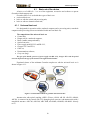
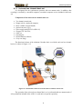
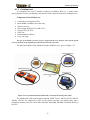
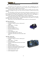
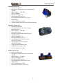
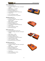
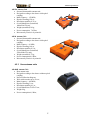
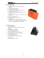
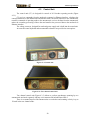
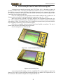
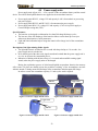
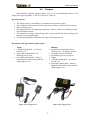
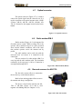
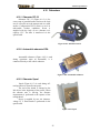
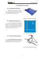
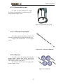

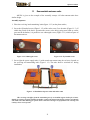
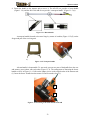
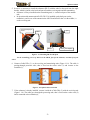
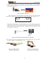
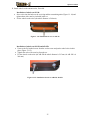
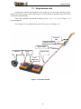
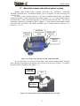
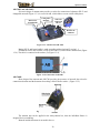
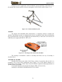
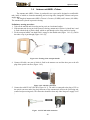
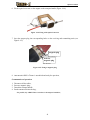
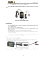
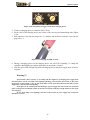
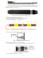
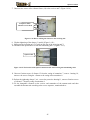
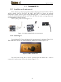
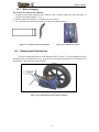
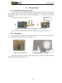
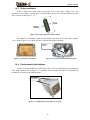
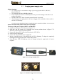
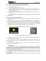
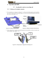
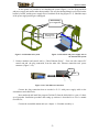
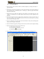
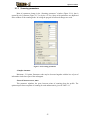
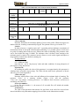
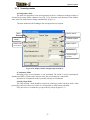
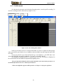
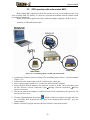
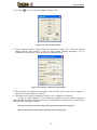
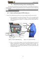
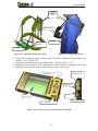
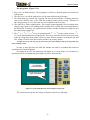
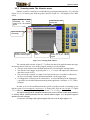
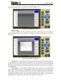

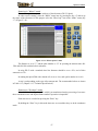
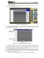
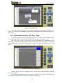
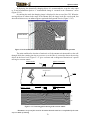
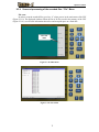
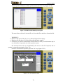
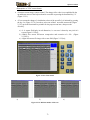
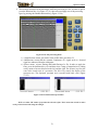
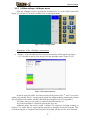
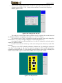
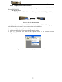
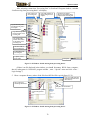
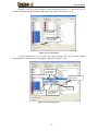
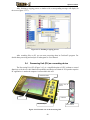
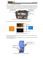
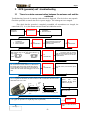
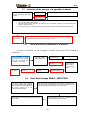
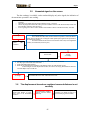
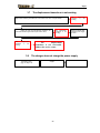
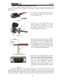
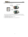
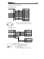
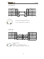
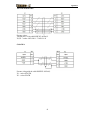
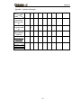
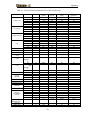
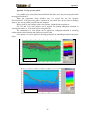
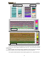


![complete information [English]](http://vs1.manualzilla.com/store/data/005803910_1-e6b0f51b61ee7060f2602055e87ee74e-150x150.png)