1
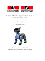
Ordinary Differential Equations Framework for
the Robotic Dog Aibo
Etienne Dysli
14th February 2005
Semester project winter 2004-2005
Supervisors: Jonas Buchli & Prof. Auke Jan Ijspeert
ii
Summary
This document is a semester project report. It presents the work done to
develop a software framework to control an Aibo robot with a set of ordinary
differential equations. The first chapter explores the ideas and the tools
which gave birth to this project. Project goals are also defined. The second
chapter describes the software engineering process that was used throughout
the project. This process follows the guidelines of the Fondue method. This
chapter also serves as developer documentation for future refactoring of the
software. The third chapter presents an example dynamical system which was
used to test and demonstrate the software. Simulation and real world results
are shown and discussed. Chapter four draws a conclusion of this project
and looks at future improvements. Finally, two appendices are provided to
bootstrap the new user into using the resulting work of this project.
Copyright information
About this document
c 2005 Etienne Dysli.
Copyright Permission is granted to copy, distribute and/or modify this document under
the terms of the GNU Free Documentation License, Version 1.2 or any later
version published by the Free Software Foundation; with no Invariant Sections, no Front-Cover Texts, and no Back-Cover Texts. A copy of the license
is included in the section entitled “GNU Free Documentation License”.
The author believes knowledge — especially scientific knowledge — should
be free (as in freedom) that is why this document is released under a license
that guarantees it will remain free.
About the software provided
Aib-O-Matic is free software; you can redistribute it and/or modify it under the terms of the GNU General Public License as published by the Free
Software Foundation; either version 2 of the License, or (at your option) any
later version.
This program is distributed in the hope that it will be useful, but WITHOUT ANY WARRANTY; without even the implied warranty of MERCHANTABILITY or FITNESS FOR A PARTICULAR PURPOSE. See the GNU
General Public License for more details.
You should have received a copy of the GNU General Public License
iii
along with this program; if not, write to the Free Software Foundation, Inc.,
59 Temple Place, Suite 330, Boston, MA 02111-1307 USA.
Trademarks
• Webots is a trademark of Cyberbotics Ltd.
• AIBO and OPEN-R are trademarks or registered trademarks of Sony
Corporation.
• “Memory Stick” is a trademark of Sony Corporation.
• Linux is a registered trademark of Linus Torvalds.
Acknowledgments
The author would like to thank Jonas Buchli and Prof. Auke Jan Ijspeert
for their support, hints and overall great help.
Special thanks to Alessandro Crespi for software installations and backup
restores.
Final thanks go to Lukas Hohl and Olivier Michel for their help with
Webots.
iv
Contents
List of Figures
1 Introduction
1.1 Motivation . .
1.2 Related work
1.3 Goals . . . . .
1.4 Outline . . . .
x
.
.
.
.
.
.
.
.
.
.
.
.
.
.
.
.
.
.
.
.
.
.
.
.
.
.
.
.
.
.
.
.
.
.
.
.
.
.
.
.
.
.
.
.
.
.
.
.
.
.
.
.
.
.
.
.
.
.
.
.
2 Software architecture
2.1 The Fondue method . . . . . . . . . . .
2.1.1 Requirements . . . . . . . . . . .
2.1.2 Analysis . . . . . . . . . . . . . .
2.1.3 Design . . . . . . . . . . . . . . .
2.1.4 Implementation . . . . . . . . . .
2.2 Environment model . . . . . . . . . . . .
2.3 Concept model . . . . . . . . . . . . . .
2.3.1 Description of analysis classes . .
2.4 Behavior model . . . . . . . . . . . . . .
2.4.1 Operation model . . . . . . . . .
2.4.2 Protocol model . . . . . . . . . .
2.5 Interaction model . . . . . . . . . . . . .
2.5.1 System operations . . . . . . . .
2.5.2 Methods . . . . . . . . . . . . . .
2.6 Dependency model . . . . . . . . . . . .
2.7 Inheritance model . . . . . . . . . . . . .
2.8 Design class model . . . . . . . . . . . .
2.9 Implementation class model . . . . . . .
2.9.1 Class TimeKeeper . . . . . . . .
2.9.2 Class DeviceController . . . . . .
2.9.3 Class Device . . . . . . . . . . . .
2.9.4 Class DynamicalSystemController
v
.
.
.
.
.
.
.
.
.
.
.
.
.
.
.
.
.
.
.
.
.
.
.
.
.
.
.
.
.
.
.
.
.
.
.
.
.
.
.
.
.
.
.
.
.
.
.
.
.
.
.
.
.
.
.
.
.
.
.
.
.
.
.
.
.
.
.
.
.
.
.
.
.
.
.
.
.
.
.
.
.
.
.
.
.
.
.
.
.
.
.
.
.
.
.
.
.
.
.
.
.
.
.
.
.
.
.
.
.
.
.
.
.
.
.
.
.
.
.
.
.
.
.
.
.
.
.
.
.
.
.
.
.
.
.
.
.
.
.
.
.
.
.
.
.
.
.
.
.
.
.
.
.
.
.
.
.
.
.
.
.
.
.
.
.
.
.
.
.
.
.
.
.
.
.
.
.
.
.
.
.
.
.
.
.
.
.
.
.
.
.
.
.
.
.
.
.
.
.
.
.
.
.
.
.
.
.
.
.
.
.
.
.
.
.
.
.
.
.
.
.
.
.
.
.
.
.
.
.
.
.
.
.
.
.
.
.
.
.
.
.
.
.
.
.
.
.
.
.
.
.
.
.
.
.
.
.
.
.
.
.
.
.
.
.
.
.
.
.
.
.
.
.
.
.
.
.
.
.
.
.
.
.
.
.
.
.
.
.
.
1
1
2
3
3
.
.
.
.
.
.
.
.
.
.
.
.
.
.
.
.
.
.
.
.
.
.
5
5
6
6
7
7
7
8
8
12
12
12
12
13
13
19
19
21
21
22
22
23
25
vi
CONTENTS
2.9.5 Class DynamicalSystem
2.9.6 Class Logger . . . . . . .
2.9.7 Class NumericalSolver .
2.9.8 Class Servo . . . . . . .
2.9.9 Class RotationServo . .
2.9.10 Class Plunger . . . . . .
2.9.11 Class Sensor . . . . . .
2.9.12 Class TouchSensor . . .
2.9.13 Class DistanceSensor . .
2.9.14 Class Camera . . . . . .
2.9.15 Class LED . . . . . . . .
2.10 Implementation quirks . . . . .
2.10.1 Known bugs . . . . . . .
3 Testing and results
3.1 Experiment setup
3.2 Results . . . . . .
3.2.1 Simulation
3.2.2 Reality . .
3.3 Discussion . . . .
.
.
.
.
.
.
.
.
.
.
.
.
.
.
.
.
.
.
.
.
.
.
.
.
.
.
.
.
.
.
.
.
.
.
.
.
.
.
.
.
.
.
.
.
.
.
.
.
.
.
.
.
.
.
.
.
.
.
.
.
.
.
.
.
.
.
.
.
.
.
.
.
.
.
.
.
.
.
.
.
.
.
.
.
.
.
.
.
.
.
.
.
.
.
.
.
.
.
.
.
.
.
.
.
.
.
.
.
.
.
.
.
.
.
.
.
.
.
.
.
.
.
.
.
.
.
.
.
.
.
.
.
.
.
.
.
.
.
.
.
.
.
.
.
.
.
.
.
.
.
.
.
.
.
.
.
.
.
.
.
.
.
.
.
.
.
.
.
.
.
.
.
.
.
.
.
.
.
.
.
.
.
.
.
.
.
.
.
.
.
.
.
.
.
.
.
.
.
.
.
.
.
.
.
.
.
.
.
.
.
.
.
.
.
.
.
.
.
.
.
.
.
.
.
.
.
.
.
.
.
.
.
.
.
.
.
.
.
.
.
.
.
.
.
.
.
.
.
.
.
.
.
.
.
.
.
.
.
.
.
.
26
29
30
31
33
33
33
33
34
34
34
35
36
.
.
.
.
.
.
.
.
.
.
.
.
.
.
.
.
.
.
.
.
.
.
.
.
.
.
.
.
.
.
.
.
.
.
.
.
.
.
.
.
.
.
.
.
.
.
.
.
.
.
.
.
.
.
.
.
.
.
.
.
.
.
.
.
.
.
.
.
.
.
.
.
.
.
.
.
.
.
.
.
.
.
.
.
.
37
37
39
39
40
41
4 Conclusions
43
4.1 Conclusion . . . . . . . . . . . . . . . . . . . . . . . . . . . . . 43
4.2 Future work . . . . . . . . . . . . . . . . . . . . . . . . . . . . 43
Bibliography
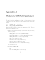
A Webots & OPEN-R Quickstart
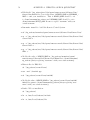
A.1 OPEN-R installation . . . . . . . . . . . .
A.2 Webots installation . . . . . . . . . . . . .
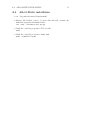
A.3 Remote Control System installation . . . .
A.3.1 Create your own Webots directory
A.3.2 Extract the world file . . . . . . . .
A.3.3 Install the Remote Control System
A.4 Aib-O-Matic installation . . . . . . . . . .
B Aib-O-Matic user manual
B.1 Installation . . . . . . . . . . . . . . . . .
B.2 How to change system parameters . . . . .
B.3 How to build your own DynamicalSystems
B.4 How to add new Devices . . . . . . . . . .
46
.
.
.
.
.
.
.
.
.
.
.
.
.
.
.
.
.
.
.
.
.
.
.
.
.
.
.
.
.
.
.
.
.
.
.
.
.
.
.
.
.
.
.
.
.
.
.
.
.
.
.
.
.
.
.
.
.
.
.
.
.
.
.
.
.
.
.
.
.
.
.
.
.
.
.
.
.
.
.
.
.
.
.
.
.
.
.
.
.
.
.
.
.
.
.
.
.
.
.
.
.
.
.
.
.
.
.
.
.
.
.
.
.
.
.
.
.
47
47
48
48
48
49
49
51
.
.
.
.
53
53
53
53
54
vii
CONTENTS
B.5 How to compile the controller . . . . . . . . . . . . . . . . . . 54
C CD-ROM table of contents
D GNU Free Documentation License
D.1 Applicability and definitions . . . . .
D.2 Verbatim copying . . . . . . . . . . .
D.3 Copying in quantity . . . . . . . . . .
D.4 Modifications . . . . . . . . . . . . .
D.5 Combining documents . . . . . . . .
D.6 Collections of documents . . . . . . .
D.7 Aggregation with independent works
D.8 Translation . . . . . . . . . . . . . .
D.9 Termination . . . . . . . . . . . . . .
D.10 Future revisions of this license . . . .
E GNU General Public License
55
.
.
.
.
.
.
.
.
.
.
.
.
.
.
.
.
.
.
.
.
.
.
.
.
.
.
.
.
.
.
.
.
.
.
.
.
.
.
.
.
.
.
.
.
.
.
.
.
.
.
.
.
.
.
.
.
.
.
.
.
.
.
.
.
.
.
.
.
.
.
.
.
.
.
.
.
.
.
.
.
.
.
.
.
.
.
.
.
.
.
.
.
.
.
.
.
.
.
.
.
.
.
.
.
.
.
.
.
.
.
.
.
.
.
.
.
.
.
.
.
.
.
.
.
.
.
.
.
.
.
.
.
.
.
.
.
.
.
.
.
57
58
59
60
61
63
63
64
64
64
65
67
viii
CONTENTS
List of Figures
2.1
2.2
2.3
2.4
2.5
2.6
2.7
2.8
2.9
2.10
2.11
2.12
2.13
2.14
2.15
2.16
2.17
2.18
2.19
2.20
2.21
2.22
2.23
2.24
2.25
2.26
2.27
Environment diagram . . . . . . . . . . . .
Simplified concept diagram . . . . . . . . .
Concept diagram . . . . . . . . . . . . . .
Protocol diagram . . . . . . . . . . . . . .
Collaboration diagram for tick . . . . . . .
Collaboration diagram for read devices . .
Collaboration diagram for update systems
Collaboration diagram for write devices . .
Dependency diagram . . . . . . . . . . . .
Inheritance diagram for Device . . . . . .
Inheritance diagram for DynamicalSystem
Design class diagram . . . . . . . . . . . .
Class TimeKeeper . . . . . . . . . . . . . .
Class DeviceController . . . . . . . . . . .
Class Device . . . . . . . . . . . . . . . . .
Class DynamicalSystemController . . . . .
Class DynamicalSystem . . . . . . . . . . .
Class Logger . . . . . . . . . . . . . . . . .
Class NumericalSolver . . . . . . . . . . .
Class Servo . . . . . . . . . . . . . . . . .
Class RotationServo . . . . . . . . . . . .
Class Plunger . . . . . . . . . . . . . . . .
Class Sensor . . . . . . . . . . . . . . . .
Class TouchSensor . . . . . . . . . . . . .
Class DistanceSensor . . . . . . . . . . . .
Class Camera . . . . . . . . . . . . . . . .
Class LED . . . . . . . . . . . . . . . . . .
3.1
3.2
3.3
Experiment setup in simulation . . . . . . . . . . . . . . . . . 38
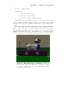
Experiment setup in reality . . . . . . . . . . . . . . . . . . . 39
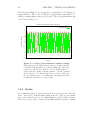
ACPO and perturbation without coupling . . . . . . . . . . . 40
ix
.
.
.
.
.
.
.
.
.
.
.
.
.
.
.
.
.
.
.
.
.
.
.
.
.
.
.
.
.
.
.
.
.
.
.
.
.
.
.
.
.
.
.
.
.
.
.
.
.
.
.
.
.
.
.
.
.
.
.
.
.
.
.
.
.
.
.
.
.
.
.
.
.
.
.
.
.
.
.
.
.
.
.
.
.
.
.
.
.
.
.
.
.
.
.
.
.
.
.
.
.
.
.
.
.
.
.
.
.
.
.
.
.
.
.
.
.
.
.
.
.
.
.
.
.
.
.
.
.
.
.
.
.
.
.
.
.
.
.
.
.
.
.
.
.
.
.
.
.
.
.
.
.
.
.
.
.
.
.
.
.
.
.
.
.
.
.
.
.
.
.
.
.
.
.
.
.
.
.
.
.
.
.
.
.
.
.
.
.
.
.
.
.
.
.
.
.
.
.
.
.
.
.
.
.
.
.
.
.
.
.
.
.
.
.
.
.
.
.
.
.
.
.
.
.
.
.
.
.
.
.
.
.
.
.
.
.
.
.
.
.
.
.
.
.
.
.
.
.
.
.
.
.
.
.
.
.
.
.
.
.
.
.
.
.
.
.
.
.
.
.
.
.
.
.
.
.
.
.
.
.
.
.
.
.
.
.
.
.
.
.
.
.
.
.
.
.
8
10
11
13
15
16
17
18
19
20
20
21
22
23
24
25
27
29
31
32
33
33
34
34
34
35
35
x
LIST OF FIGURES
3.4
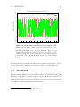
ACPO and perturbation with coupling . . . . . . . . . . . . . 41
Chapter 1
Introduction
In this chapter, we briefly explore the ideas and the tools which gave birth
to this project. Project goals are also defined here.
1.1
Motivation
From equations to life
Non-linear dynamical systems offer new and creative possibilities for the control of locomotion in legged robots. Their interesting properties include resistance to perturbations, attractors and synchronization with other systems
or external input. These properties can be exploited to design a new generation of robot controllers: “online” controllers. These are truly reactive
and can adapt themselves to their environment, as opposed to programmed
controllers. They can react to every situation, even unplanned ones.
However, the search space of dynamical system parameters is huge. So
finding the right system parameters to obtain a given property is far from
being trivial. To explore the immense space of possible configuration, it would
be desirable to have software tools to test one’s ideas both in simulation and
on a real robot.
The structure of non-linear dynamical systems bears some level of similarity with the neural structure of living beings. A dynamical system itself
can be a collection of many dynamical systems. These systems are linked
together and with the robot’s sensors and actuators. They can be thought
of as a collection of neurons, a “brain”, which generates signal patterns in
response to sensory input. This approach might be useful to understand how
the neural system of animals and humans work. Or it can be used to produce
very animal-like robot behavior, featuring adaptive locomotion and learning
capabilities.
1
2
CHAPTER 1. INTRODUCTION
A sympathetic yet powerful dog
The robotic dog Aibo is made by Sony. It is marketed both as an entertainment system and as a research platform. Aibo features plenty of sensors
(color camera, infrared distance sensor, chin, back and paw touch sensors)
and actuators (LEDs and head, leg, ear, and tails joints). Sony provides a
free development kit, the OPEN-R SDK, based on the GNU Compiler Collection (gcc) to write software for the Aibo. OPEN-R allows cross-compiling
programs on a PC to run them on the Aibo.
Simulators are helpful to try new software without taking the risk of
breaking real robots. Simulation is also faster than real world experiments.
Webots, a commercial mobile robot simulation software developed by Cyberbotics Ltd [1] includes support for the Aibo. It features an Aibo model
and a graphical user interface to observe and control the robot’s parameters
(both in simulation and on the real Aibo via a wireless link). One can also
transfer programs from the PC to Aibo’s memory with a single click.
1.2
Related work
Previous work in the field of biologically-inspired robotics contribute to the
initial spark of this project.
Central pattern generators and quadrupedal locomotion In their
article “Hard-wired central pattern generators for quadrupedal locomotion”
[2] Collins and Richmond set the grounds of central pattern generators (CPG)
used to control the locomotion of quadrupeds. Jonas Buchli and Auke Jan
Ijspeert further extend the topic to differential systems in [3]. A system made
of amplitude controlled phase oscillators (ACPO) will be implemented to test
and demonstrate the final program.
Aibo simulation and transfer to real robot First and foremost, the two
semester projects made by Lukas Hohl during the previous year provide the
toolbox needed to develop control software for the Aibo. In [4] he presents
the “Remote Control System” which allows monitoring and controlling an
Aibo robot from a PC over a wireless connection. Then he integrated this
software into Webots allowing the same monitoring to be performed both on
a simulated and a real Aibo. Moreover, in [5], he added the cross-compiling
function of OPEN-R to the graphical interface of Webots. This greatly helps
the development of Aibo control software, as one is now able to write a single
1.3. GOALS
3
program which runs both in Webots and on the real Aibo using the Webots
Controller API.
Quadruped locomotion controllers based on non-linear oscillators
Mathieu Salzmann explored controllers based on non-linear oscillators to generate different gaits in quadruped locomotion. In [6] he shows how to have
transitions between the different gaits by changing only one parameter in the
differential equations of the controllers. He used a simulated Aibo in Webots
in his experiments. His work shows that it is possible to implement natural
movements (e.g. walk, trot and bound) with non-linear oscillators.
Self-organization of locomotion In his study of “Self-Organization of
Locomotion in Modular Robots” [7], Bertrand Mesot uses genetic algorithms
to tune oscillators toward sensible movement patterns. This suggests we
could do the same to find interesting parameters of dynamical systems.
1.3
Goals
Up to now, only simulation and pre-calculated trajectories have been used
to test non-linear systems in quadruped locomotion. We now have the tools
to test the same controller program in both simulated and real environment.
The aim of this project is to develop a software framework allowing to
control the Aibo robot with a set of dynamical systems. The robot running
this system shall be independent of any other external processor, in particular
it shall not get any help from a PC to solve differential equations. The same
code must be used both in simulation and on the real robot.
1.4
Outline
The initial plan for this project was:
• Test Webots & OPEN-R integration and cross-compilation. This amounts
to using and testing Lukas Hohl’s software (see [4, 5]).
• Develop an ordinary differential equations (ODE) framework to allow
control of Aibo via non-linear dynamical systems. The code should be
the same for simulation and real world runs.
• Interactively demonstrate that the Aibo is controlled by a dynamical
system.
4
CHAPTER 1. INTRODUCTION
• Write a user manual of the developed software.
Chapter 2
Software architecture
This chapter describes the software engineering process that I have used
throughout my project. This process follows the guidelines of the Fondue
method I learned in a software engineering course given by Prof. Alfred
Strohmeier. I choose to use this method because writing code without planning first is a bad thing and it is the only method I already know since I
practiced it during the software engineering project. Employing this method
also has the advantage of documenting the software itself while designing it,
which is important for users and future developments.
2.1
The Fondue method
What is Fondue? From [8]:
Fondue is a software development method for reactive systems.
Fondue evolved from the Fusion method, originally defined by
Derek Coleman. It keeps the process and the models of the original Fusion method but uses the UML for the notation.
The Fondue process has four phases: requirements elicitation, analysis,
design and implementation. The first phase defines what the software is
required to do. The analysis phase turns the requirements into a specification.
The design phase turns this specification into an architecture. And finally the
implementation phase maps this architecture to a programming language. I
will briefly explain these phases to give the reader enough background to
understand the following models. The interested reader might want to read
[9] for a detailed description of the method.
5
6
2.1.1
CHAPTER 2. SOFTWARE ARCHITECTURE
Requirements
The requirements phase produces two models: use cases and the domain
model out of a textual or oral description of the software. A use case describes possible situations that can arise when a user has a particular goal
against the system. It is an informal, mainly textual, goal-based description
which captures the behavioral requirements of the software system. The domain model captures the concepts in the domain of the problem, and the
relationships between them. It uses a class diagram notation.
I have skipped this phase in my project because my system is not an
interactive one in the sense that its actions are not triggered by an input
from a human user. Of course the Aibo robot has be able to react to sensory
perception such as the activation of a paw touch sensor (which might be
triggered by human intervention) but there is no real user interface to a
human user. Classifying my system as “non reactive” makes it degenerated
from the point of view of Fondue. Some models loose their raison d’être
because they are intended to describe user-system interaction or depend on
user input.
The only user intervention at run time is switching on the robot or launching a simulation in Webots. Then all inputs happen through the robot’s devices. There would be only a single use case, boiling down to “switch robot
on”. Therefore, use cases are not needed. The domain model closely, if not
exactly, resembles the concept model to be seen in the next phase. I decided
to draw it only once.
2.1.2
Analysis
The analysis phase generates five models:
Environment model The environment is the set of actors with which the
system communicates, via messages. This model uses a collaboration
diagram to model the interactions between the actors and the system.
It is defined by the set of input messages the system can receive, the
set of time-triggered input events, the set of operations the system can
perform and the set of it can output.
Concept model The concept model is a subset of the domain model. It
keeps only what is part of the system. Everything else belonging to the
environment is left out. It contains the set of classes and associations
modeling the system state.
Behavior model The behavior model is the addition of the protocol model
and the operation model.
2.2. ENVIRONMENT MODEL
7
Operation model The operation model uses the Object Constraint
Language (OCL, see [10]) to specify the effects of operations in
terms of system state changes and output messages sent.
Protocol model The protocol model defines the allowable sequence of
operations during the lifetime of the system. It is a state diagram.
2.1.3
Design
The design phase aims to develop an object-oriented system architecture that
satisfies the requirements defined during the analysis phase. It also provides
the foundations of the implementation, testing and maintenance. All information and relationships defined in the concept model must be preserved.
This results in a collection of interacting objects which realizes the operation
model. This phase yields four models:
Interaction model The interaction model shows how objects interact at
run-time to support the functionality specified in the operation model.
Dependency model The dependency model describes dependencies between classes and communication paths between interacting objects.
Inheritance model The inheritance model describes the superclass/subclass
inheritance design structure.
Design class model The design class model is composed of the contents
of all design classes (their attributes and methods), all the navigable
associations between design classes and the inheritance structure.
2.1.4
Implementation
The work to be done in this phase relies on the interaction model and the
design class model. The class interface has to be defined as well as the
visibility of attributes/methods and whether a method or class is abstract or
not. This will yield the implementation class model.
Finally code writing can take place. One has just to follow the implementation class model using an object-oriented programming language.
2.2
Environment model
The environment is very simplified because the system is not interactive.
There is one user actor, only one input message run and one time-triggered
message tick.
8
CHAPTER 2. SOFTWARE ARCHITECTURE
run()
:Aib-O-Matic
<<time-triggered>> tick()
:User
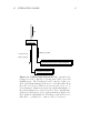
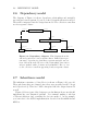
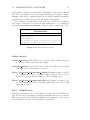
Figure 2.1: Environment diagram The environment diagram is very simple because there are only two messages: run
and tick. The user starts the system and then the system runs on
its own at the beat of tick messages.
run() Launches the system1 .
tick() Updates readings from devices, solves dynamical systems and applies
results to devices. This message is triggered at each simulation step.
2.3
Concept model
As already said, the concept model is similar to the domain model. Note
that there are no actors, nor classes representing actors inside the system.
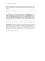
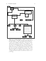
Everything is in the system, it is called a simulation model. Figure 2.3
shows the full concept model and Figure 2.2 shows the same model without
inheritance which makes it (hopefully) easier to read.
2.3.1
Description of analysis classes
Here is the verbal description of the classes depicted on Figures 2.2 and 2.3
(pages 10–11).
Class TimeKeeper Knowing the current time is essential to the operation
of the NumericalSolver from where the existence of the TimeKeeper class. It
maintains a clock reference and takes care of updating the Devices and the
DynamicalSystems regularly, that is at each time step.
Class Device The Device class is a generic representation of all the sensors
and actuators of the robot. It offers basic capabilities like reading, writing,
1
Starting the system is not covered by Fondue. From this point of view, run is not
really a message so it won’t be covered in the analysis phase. Of course objects have to
be created at system startup thus run will appear again in the implementation phase.
2.3. CONCEPT MODEL
9
buffering, normalizing values, and enabling/disabling. It is meant to be extended via subclasses to represent more precise peripherals like servos and
sensors.
Class DynamicalSystem The DynamicalSystem class is burdened with
the representation of ODE systems: equations, state variables, parameters,
initial conditions, names and a selection of variables to export for external
use. There will be one instance of this class per differential system to facilitate the definition of the systems by the user. But, mathematically, the
collection of differential systems can be seen as one single system and will be
treated as such at the time of numerical solving. It has the ability to read
and write to any Device. It can also read other DynamicalSystem’s state
variables. This serves the need of introducing coupling between systems and
also between the robot’s devices and the various dynamical systems. Finally,
DynamicalSystems employ the NumericalSolver class to solve their equations.
Class Logger The Logger class has no associations leading to it because it
has only a single instance and thus enjoys system-wide visibility. In the other
direction, it also doesn’t need any association with other classes because it
won’t use them. The Logger ’s purpose is to provide a facility to log error or
information messages and to output system data (i.e. the DynamicalSystems’
state variables) for external use.
10
CHAPTER 2. SOFTWARE ARCHITECTURE
<<system>>
Aib-O-Matic
theclock
1
TimeKeeper
1
1
theclock
updates systems
rtc: time
1..*
systems
mycontroller
0..*
DynamicalSystem
1..*
systems
0..*
name: string
variables: real[]
parameters: real[]
variable_names: string[]
output_variables: boolean[]
updates buffers
mysystems
0..*
reads
reads & writes
1..*
NumericalSolver
devices
1..*
Device
name: string
tag: DeviceTag
enabled: boolean
buffer: real
1..*
mysolver
1
mydevices
0..*
Logger
1
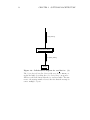
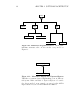
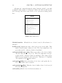
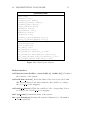
Figure 2.2: Simplified concept diagram Concept diagram
shown without inheritance relationships. This model captures the
initial idea of the system’s classes and their interaction.
Knowing the current time is essential to the NumericalSolver from
where the existence of the TimeKeeper class. It maintains a clock
reference and takes care of updating the Devices and the DynamicalSystems regularly. The Device class represents all the sensors
and actuators of the robot. It offers basic capabilities like reading,
writing, buffering, normalizing values, and enabling/disabling.
The DynamicalSystem class is burdened with the representation
of differential systems. It has the ability to read and write to any
Device, it can also read other DynamicalSystem’s state variables.
Finally, it employs the NumericalSolver class to solve it’s equations. The Logger class has no associations leading to it because it
enjoys system-wide visibility. It’s purpose is to provide a facility
to log error or information messages and to output system data
for external use.
uses
11
2.3. CONCEPT MODEL
<<system>>
Aib-O-Matic
TimeKeeper
1
1
theclock
updates systems
rtc: time
1..*
systems
theclock
1
updates buffers
mycontroller
0..*
1..*
DynamicalSystem
systems
*
name: string
variables: real[]
parameters: real[]
variable_names: string[]
output_variables: boolean[]
reads & writes
devices
1..*
Device
1..*
mysystems
0..*
mydevices
0..*
name: string
tag: DeviceTag
enabled: boolean
buffer: real
reads
Logger
Camera
Sensor
TouchSensor
uses
1..*
1
NumericalSolver
LED
DistanceSensor
mysolver
1
Servo
position_current: real
position_min: const real
position_max: const real
position_init: const real
velocity_current: real
velocity_min: const real
velocity_max: const real
velocity_init: const real
acceleration_current: real
acceleration_min: const real
acceleration_max: const real
acceleration_init: const real
force_current: real
RotationServo
Plunger
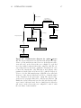
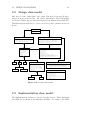
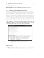
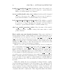
Figure 2.3: Concept diagram Complete concept model including inheritance relationships. The upper half of this figure is
the same as Figure 2.2. The lower half shows the subclass “tree”
of Device as it is planned at this stage of the process. These
classes (Camera, TouchSensor, DistanceSensor, LED, Servo, RotationServo) are all inspired by Webots’ controller API. Servo and
RotationServo are essentially the same save their treatment of
numbers: the former’s base unit is meters and the latter’s is radians. Sensor is a generic representation of a sensor device. It has
little interest in itself except that it forbids writing to sensors. A
Plunger is a limited servo which has only two positions: on and
off. This class
P stems from Aibo’s ears which are restricted to two
positions.
12
2.4
CHAPTER 2. SOFTWARE ARCHITECTURE
Behavior model
Last model of the analysis phase, the behavior model is the addition of the
protocol model and the operation model. It expresses the behavior of the
system regarding input messages. The operation model states what the effect
of messages are. It serves as a base to write program code later. The protocol
model defines the authorized sequence of messages.
2.4.1
Operation model
The OCL is not easy to read if you don’t know it. That’s why pre- and
post-conditions are expressed in plain English rather than in OCL.
Operation schema of “tick”
Operation: Aib-O-Matic::{tick()};
Description: Advance the simulation by one time step.
Scope: TimeKeeper, Device, DynamicalSystem, NumericalSolver;
Pre: true;
Post: Read the input of all devices.
Solve the dynamical system.
Write the output of the dynamical system to the devices.
2.4.2
Protocol model
Due to the low number of messages, the protocol model is very simple (Figure
2.4, page 13). The run operation starts the system and brings it in the
“running” state. Once it is running, it keeps on running with tick and it
is the only thing it can do. There is no provision for stopping the system
because the controller program will simply be unloaded from memory by
Webots (in simulation) or by Aibo’s operating system (on the real robot) at
shutdown.
2.5
Interaction model
Here begins the design phase. The interaction model details what operations
and methods do: how objects interact to realize what has been specified in
the previous phase. Message order is specified via Dewey numbers on the
collaboration diagrams.
13
2.5. INTERACTION MODEL
tick
run
running
system
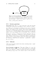
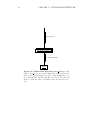
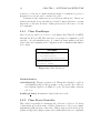
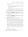
Figure 2.4: Protocol diagram The run operation starts the
system. Once it is running, it keeps on running with tick. There
is no provision for stopping the system because the controller program will simply be unloaded from memory by Webots or by
Aibo’s operating system at shutdown.
2.5.1
System operations
Aib-O-Matic::tick Figure 2.5 on page 15 shows the collaboration diagram
describing the operation tick. It is triggered by the controller loop robot_run of Webots at each simulation step (function robot_run is documented
in [11]). The TimeKeeper is the controller of this operation. It first instructs
all Devices to read their values from the real robot’s devices. This is done via
a special object: a “collection manager” which is represented as a particular
instance of the class it manages, here deviceController: Device. Collection
managers are a new type of class introduced in the design phase. They are
very useful to send messages to all instances of the same class, to insert and
remove instances, and to browse or search them. Likewise, all DynamicalSystems are told to update themselves, that is solve their equations. Finally,
the TimeKeeper tells all Devices to write their — possibly new — values to
the robot’s devices.
2.5.2
Methods
Collaboration diagram for methods show what certain important or complicated methods shall do.
DeviceController::read devices This method (Figure 2.6 on page 16)
triggers the reading of every robot device in the system by the corresponding
Device object. Each Device instance holds the latest value read in a buffer.
The buffer speeds up access to device values because no call to the Webots
14
CHAPTER 2. SOFTWARE ARCHITECTURE
API is needed. It also prevents different values of the same device to be read
in one time step. This ensures consistency of the values during a simulation
step. Hence the robot’s status is made available to the controller program.
DynamicalSystemController::update systems This is one of the most
important methods of the whole program. This method is responsible for
telling every DynamicalSystem to read from it’s input Devices (if any), launching the NumericalSolver to solve the system, and writing the new values of
state variables to the DynamicalSystems and their output Devices (if any).
The collaboration diagram of update systems is depicted on Figure 2.7, page
17.
The dynamicalSystemController first tells all DynamicalSystems to read
from their associated Devices. That is what they immediately do by calling
read() on the Devices they are configured to read. They store the returned
values in their state variables. The dynamicalSystemController then consults
the TimeKeeper in order to know the current time. This time is used (among
other parameters detailed later in section 2.9.7) to ask the NumericalSolver
to solve the differential system. The solver calls back derivate() of the dynamicalSystemController to obtain the values of the derivatives at the given
time. The latter propagates this call to each DynamicalSystem. Note that
solve() is called multiple times during a single simulation step because the
solver advances with smaller steps than the simulation. Finally the dynamicalSystemController tells each DynamicalSystem to write to their associated
Devices. They call write() on the Devices they are configured to write to
with the new values of their variables.
DeviceController::write devices Similarly to read devices seen earlier,
this method (Figure 2.8 on page 18) triggers the writing of every Device’s
buffer into the corresponding robot device, thus making the robot move, act
and generally react to its environment.
15
2.5. INTERACTION MODEL
tick()
: TimeKeeper
2: update_systems()
1: read_devices()
3: write_devices()
dynamicalSystemController: DynamicalSystem
deviceController: Device
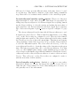
Figure 2.5: Collaboration diagram for tick Operation tick
is triggered by the controller loop robot_run of Webots at each
simulation step. The TimeKeeper is the controller of this operation. (1) It first instructs all Devices to read their values from
the real robot’s devices. This is done via a special object: a “collection manager” which is represented as a particular instance of
the class it manages, here deviceController: Device. (2) Likewise,
all DynamicalSystems are told to update themselves, that is solve
their equations. (3) Finally, the TimeKeeper tells all Devices to
write their — possibly new — values to the robot’s devices.
16
CHAPTER 2. SOFTWARE ARCHITECTURE
read_devices()
deviceController: Device
1*: update_buffer()
: Device
*
Figure 2.6: Collaboration diagram for read devices (1)
The object deviceController: Device tells every Device instance to
update its buffer by reading the robot device they correspond to.
All Devices hold the latest value they’ve read in a buffer. The star
next to the message number denotes the fact that the message is
sent to multiple objects.
17
2.5. INTERACTION MODEL
update_systems()
3.2*: derivate(...)
4*: write_to_devices()
*
: DynamicalSystem
dynamicalSystemController: DynamicalSystem
4.1*: write(...)
2: get_time()
3.1: derivate(...)
1*: read_from_devices()
mydevices: Device
*
theclock: TimeKeeper
3: solve(...)
: DynamicalSystem
*
mysolver: NumericalSolver
1.1*: read()
mydevices: Device
*
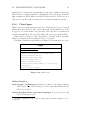
Figure 2.7: Collaboration diagram for update systems
(1) The dynamicalSystemController first tells all DynamicalSystems to read from their associated Devices. (1.1) DynamicalSystems call read() on the Devices they are configured to read and
store the returned values in their state variables. (2) The dynamicalSystemController then consults the TimeKeeper in order
to know the current time. (3) This time is used (among other
parameters detailed later in section 2.9.7) to ask the NumericalSolver to solve the differential system. (3.1) The solver calls back
derivate() of the dynamicalSystemController to obtain the values
of the derivatives at the given time. (3.2) The dynamicalSystemController propagates this call to each DynamicalSystem. (4)
Finally the dynamicalSystemController tells each DynamicalSystem to write to their associated Devices. (4.1) DynamicalSystems
call write() on the Devices they are configured to write to with
the new values of their variables.
18
CHAPTER 2. SOFTWARE ARCHITECTURE
write_devices()
deviceController: Device
1*: writeback_buffer()
: Device
*
Figure 2.8: Collaboration diagram for write devices Similarly to read devices seen earlier, this method makes all Devices
write to the corresponding robot device, thus making the robot
move (among other actions). (1) The deviceController tells each
Device to write the value of its buffer to the associated robot device.
19
2.6. DEPENDENCY MODEL
2.6
Dependency model
The diagram of Figure 2.9 shows dependency relationships and navigable
associations between system objects as deduced from the interaction model.
They will be integrated into the design class model. The collection controllers
are now separate classes.
<<call>>
TimeKeeper
theTK
1
theDSC
1
DeviceController
devices
1..*
mydevices
Device
0..*
DynamicalSystemController
systems
1..*
DynamicalSystem
dsc
1
mysolver
1
NumericalSolver
Figure 2.9: Dependency diagram This diagram shows the
various dependencies between system classes. Dashed lines represent usage dependencies, plain lines represent navigable associations. Arrows show the direction of the relationships. Association
ends are marked with role names and cardinalities. Here we can
see the collection controllers appearing clearly as separate classes.
2.7
Inheritance model
The inheritance structure of class Device is shown on Figure 2.10, page 20.
These subclasses have not changed since they were presented in the concept
model (section 2.3). This “tree” will be integrated into the design class model
as well.
Figure 2.11 is not part of the design process but hints at how a user should
implement his own dynamical systems. I recommend making a subclass
of DynamicalSystem and overriding the derivate method. As an example,
you can refer to the ACPO implementation described in files ACPO.hh and
ACPO.cc.
20
CHAPTER 2. SOFTWARE ARCHITECTURE
Device
Camera
TouchSensor
Sensor
LED
Servo
DistanceSensor
RotationServo
Plunger
Figure 2.10: Inheritance diagram for Device It is the same
inheritance structure as the one shown in the concept model on
Figure 2.3.
DynamicalSystem
ExampleOscillator
Figure 2.11: Inheritance diagram for DynamicalSystem
This is the recommended way of implementing your own differential systems. Make a subclass of DynamicalSystem and override
the derivate method. As an example, you can refer to the ACPO
implementation described in files ACPO.hh and ACPO.cc.
21
2.8. DESIGN CLASS MODEL
2.8
Design class model
Last model of the design phase, the design class model regroups all information from previous models. All classes, inheritances and relationships
are shown. Classes appear with their methods but without their attributes.
Trivial navigation methods (i.e. getters and setters) and constructors are not
shown.
<<call>>
theTK
1
TimeKeeper
tick(in dt:int)
get_time(): double
theDSC
1
DeviceController
update_systems()
derivate(in time:double,in x:double[],out dx:double[])
get_DS_by_index(in index:size_t): DynamicalSystem*
get_DS_by_name(in name:char[]): DynamicalSystem*
set_TimeKeeper(in t:TimeKeeper*)
devices
1..*
Device
dsc
1
DynamicalSystemController
read_devices()
write_devices()
get_device_by_index(in index:size_t): Device*
get_device_by_name(in name:char[]): Device*
systems
1..*
mydevices
0..*
DynamicalSystem
read(): double
write(in value:double)
update_buffer()
writeback_buffer()
enable()
disable()
get_name(): char*
derivate(in t:double,in x:double[],out dx:double[])
read_from_devices()
write_to_devices()
get_name(): char*
get_dimension(): size_t
get_variable(in index:size_t): double
set_variable(in value:double,in index:size_t)
get_output_variable_state(in index:size_t): bool
get_variable_name(in index:size_t): char*
mysolver
1
Camera
TouchSensor
Sensor
LED
DistanceSensor
Servo
NumericalSolver
read_position(): double
read_velocity(): double
read_acceleration(): double
write_position(in value:double)
write_velocity(in value:double)
write_acceleration(in value:double)
enable_motor()
disable_motor()
RotationServo
Plunger
log_line(in dimension:size_t,in time:double,
in data:double[],in mask:bool[])
solve(in x:double[],inout dx:double[],in dimension:size_t,
in t:double,in h:double,out output_x:double[],
in output_interval:int,in output_variables:bool[])
Logger
log(in level:LogLevel,in message:char[])
error(in message:char[])
warning(in message:char[])
info(in message:char[])
debug(in message:char[])
output_data(in data:double[],in size:size_t)
flush_data()
get_instance(): Logger*
Figure 2.12: Design class diagram
2.9
Implementation class model
The implementation classes are described in this section. Their attributes
and methods are shown along with their visibility. According to the UML
22
CHAPTER 2. SOFTWARE ARCHITECTURE
notation, a - in front of a name means the method or attribute is private, a
# means it is protected, and a + means it is public.
Constructors and destructors are not shown in this model. Private attributes and methods are generally not described unless they have a certain
importance to the user. For more details, please refer to the source code and
it’s comments.
2.9.1
Class TimeKeeper
Since it is not possible, as of now, to read Aibo’s Real Time Clock (RTC)
through the Webots API this class has been designed to maintain a clock
reference. At each simulation step, it counts how many milliseconds have
elapsed since the beginning of the computation and accumulates this number
in a counter.
TimeKeeper
-rtc: unsigned long
-dc: DeviceController*
-dsc: DynamicalSystemController*
+tick(in dt:int)
+get_time(): double
Figure 2.13: Class TimeKeeper
Method interface
void tick(int dt) Triggers operation tick. This method should be called at
each simulation step for the program to work correctly. It’s collaboration diagram (depicted on Figure 2.5, page 15) shows what operation
tick does.
double get time() Returns the elapsed time in seconds.
2.9.2
Class DeviceController
This class is responsible for managing the collection of Devices. It allows
looking them up by their name or index. References to Devices are simply
implemented with an array of fixed size. Thus lookup by index is fast (complexity is O(1)) but lookup by name can be inefficient (worst case complexity
2.9. IMPLEMENTATION CLASS MODEL
23
is O(n) where n is the size of the array). A hash table could be more efficient
here. Since the number of devices is rather small (32), the burden of implementing a hash table to manage them is not worth the (small) performance
gain. Therefore, hash tables were left out during development.
The constructor of this class creates all Device objects. If one wants to
add, remove or modify robot devices it is the right place to do it. Numerical
data such as maximum and minimum positions of servos come from [5, 12].
DeviceController
-devices: Device**
+read_devices()
+write_devices()
+get_device_by_index(in index:size_t): Device*
+get_device_by_name(in name:char[]): Device*
Figure 2.14: Class DeviceController
Method interface
void read devices() Tell all Devices to read the value of their associated
robot device and to put it into their buffer.
void write devices() Tell all Devices to write the value stored in their
buffer into the corresponding robot device.
Device* get device by index(size t index) Returns a pointer to the Device designated by index. Returns a null pointer if index is out of
bounds (i.e. greater than the number of Devices minus one).
Device* get device by name(const char* n) Returns a pointer to the
Device designated by name n. Returns a null pointer if no Device with
this name is found.
2.9.3
Class Device
This class represents a device of the Aibo robot inside the Aib-O-Matic system. Devices can be any input or output mechanism from servos to cameras.
This class provides basic I/O functionalities and is meant to be sub-classed
to represent more specific devices with more capabilities.
24
CHAPTER 2. SOFTWARE ARCHITECTURE
All input and output through the method interface should occur with
normalized values in the [−1; 1] interval. Calls to the Webots API use the
float data type and Device uses double, a loss of precision is thus possible
here.
Device
#name: char[]
#tag: DeviceTag
#enabled: bool
#buffer: double
+read(): double
+write(in value:double)
+update_buffer()
+writeback_buffer()
+enable()
+disable()
+get_name(): char*
Figure 2.15: Class Device
Method interface All methods are declared virtual to allow them to be
inherited.
double read() Returns the value of the device stored in its buffer. This
method should return a value in [−1; 1]. The device must have been
previously enabled, otherwise behavior is undefined.
void write(double new value) Write a new value to the device’s buffer.
The new value should be in [−1; 1]. The device must have been previously enabled, otherwise behavior is undefined. The change in the
buffer is not propagated to the real device. This has to be explicitly
done with the writeback buffer method.
void update buffer() Read from the robot’s device and update the device’s buffer if the device is enabled.
void writeback buffer() Write the device’s buffer to the robot’s device (if
the device is enabled).
void enable() Enable device feedback, movement, etc.
2.9. IMPLEMENTATION CLASS MODEL
25
void disable() Disable the device.
char* get name() Returns the human readable name of the device.
2.9.4
Class DynamicalSystemController
This class is responsible for managing the collection of DynamicalSystems.
It allows looking up a DynamicalSystem by its name or index. References to
the DynamicalSystems are simply implemented with an array of fixed size.
Thus lookup by index is fast (complexity is O(1)) but lookup by name can
be inefficient (worst case complexity is O(n) where n is the size of the array).
A hash table could be more efficient here. Again, if the number of dynamical
systems is small, implementing a hash table might not be worth the effort.
If your system does have a lot of differential systems, you might look into it
though
The constructor of this class creates all DynamicalSystem objects. All
dynamical systems have to be specified in this constructor. This is the part
of the program that the user has to edit to run his own systems.
DynamicalSystemController
-total_dimension: size_t
-output_variables: bool[]
-output_names: char[][]
-output_interval: int
-mysolver: NumericalSolver*
-dc: DeviceController*
-tk: TimeKeeper*
-systems: DynamicalSystem**
+update_systems()
+derivate(in time:double,in x:double[],out dx:double[])
+get_DS_by_index(in index:size_t): DynamicalSystem*
+get_DS_by_name(in name:char[]): DynamicalSystem*
+set_TimeKeeper(in t:TimeKeeper*)
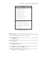
Figure 2.16: Class DynamicalSystemController
Method interface
void update systems() Update all DynamicalSystems. This method is
the workhorse of Aib-O-Matic. You might want to have a look at it’s
26
CHAPTER 2. SOFTWARE ARCHITECTURE
collaboration diagram (Figure 2.7, page 17) for a visual representation
of what it does.
1. Tell all DynamicalSystems to read values from their devices (if
they need to) and gather all state variables into one big array
that will be passed to the solver.
2. Launch the solver.
3. Write back state variables into their respective systems and tell
all DynamicalSystems to write to their devices (if they need to).
void derivate(const double t, const double x[], double dx[]) Derivate
all DynamicalSystems. Should only be called by the NumericalSolver.
DynamicalSystem* get DS by index(size t index) Returns a pointer
to the DynamicalSystem designated by index. Returns a null pointer
if index is out of bounds (i.e. greater than the number of DynamicalSystems minus one).
DynamicalSystem* get DS by name(const char* n) Returns a pointer
to the DynamicalSystem designated by name n. Returns a null pointer
if no system with this name is found.
void set TimeKeeper(TimeKeeper* t) Sets the reference to the TimeKeeper. Should only be called once at system startup.
This is a workaround to the “chicken and egg” problem: the TimeKeeper
needs a reference to the DynamicalSystemController and vice-versa. So
the DynamicalSystemController is created first then the TimeKeeper
(with a reference to the DynamicalSystemController ) and finally a reference to the TimeKeeper is given to the DynamicalSystemController.
This is more of a hack than a satisfactory solution. One should have a
look at design patterns [13] to find a better answer to this problem.
It might seem that this problem is solvable by using the Singleton design pattern. Since this requires private constructors it is incompatible
with constructors that accept parameters. So that rules the Singleton
out. Moreover doing without constructors is not the good way to initialize object references in my opinion. But some hope may reside in
Factories. . .
2.9.5
Class DynamicalSystem
This class represents a non-linear dynamical system. It is not abstract but
is expandable nonetheless — remember Figure 2.11.
2.9. IMPLEMENTATION CLASS MODEL
27
DynamicalSystem
#name: char[]
#dimension: size_t
#variables_init: double[]
#variables_current[]: double[]
#variables_names: char[][]
#output_variables: bool[]
#parameters: double[]
#nb_parameters: size_t
#mydevices: Device**
#nb_devices: size_t
#variable_to_device_mapping: bool[][]
#device_to_variable_mapping: bool[][]
+derivate(in t:double,in x:double[],out dx:double[])
+read_from_devices()
+write_to_devices()
+get_name(): char*
+get_dimension(): size_t
+get_variable(in index:size_t): double
+set_variable(in value:double,in index:size_t)
+get_output_variable_state(in index:size_t): bool
+get_variable_name(in index:size_t): char*
Figure 2.17: Class DynamicalSystem
Method interface
void derivate(const double t, const double x[], double dx[]) Calculates
the derivative of the system.
void read from devices() Reads the values of the devices associated with
this DynamicalSystem and writes them into his variables according to
the device to variable mapping.
void write to devices() Write the variables to the corresponding devices
according to the variable to device mapping.
char* get name() Returns the name of the system.
size t get dimension() Returns the system’s dimension (i.e. the number
of state variables).
28
CHAPTER 2. SOFTWARE ARCHITECTURE
double get variable(size t index) Returns the value of the variable designated by index. If index is out of bounds (i.e. greater than the
number of variables minus one), returns 0.
int set variable(double value, size t index) Sets the variable designated
by index to the given value. Returns 1 if index is out of bounds (i.e.
greater than the number of variables minus one), 0 otherwise.
bool get output variable state(size t index) Tells whether a variable
is selected for data output. Returns true if the variable designated
by index is to be logged. Returns false otherwise or if index is out of
bounds (i.e. greater than the number of variables minus one).
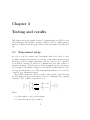
char* get variable name(size t index) Gives the name of the variable
designated by index. Returns a string if the name exists or a null
pointer otherwise.
How to make your own dynamical systems First create a subclass of
DynamicalSystem which overrides method derivate. Inside this method, you
can implement your own equations. You have get DS by index and get DS by name from the DynamicalSystemController at your disposal to find other
systems and get variable to read their variables. Please refrain from doing
anything else than reading to other DynamicalSystems, otherwise they will
certainly start to behave in an unexpected manner.
Likewise, you can connect your systems with I/O devices by setting the
two boolean arrays variable to device mapping and device to variable mapping at instantiation. variable to device mapping is first indexed by variable
number and then by device number. Meaning that if the element variable_to_device_mapping[x][y] is true, variable number x will get written
to device number y after the system has been solved. device to variable mapping is the reverse: it is indexed first by device number and then by variable
number. Meaning that if the element device_to_variable_mapping[x][y]
is true, the value of device number x will get written to variable number y
before the system is solved. You can set those two arrays to null if you don’t
use them.
Right after writing the above paragraphs, I realized that the coupling
between dynamical systems had been badly designed. The coupling is frozen
in the derivate method with no way to specify it elsewhere (for instance at
object creation). Because of that, the user has to create one class for each
DynamicalSystem even if they only differ in their coupling. If one has a lot
of systems, this will be cumbersome. That design flaw makes Aib-O-Matic
2.9. IMPLEMENTATION CLASS MODEL
29
unsuitable for evolutionary experiments because the coupling between systems cannot be changed without recompiling the whole program. Desirable
improvements for Aib-O-Matic now include refactoring it to fit the needs of
GAs and to ease the task of creating lots of identical dynamical systems.
2.9.6
Class Logger
Utility class for logging messages and data. Messages are logged to stdout
when run in Webots and to the console when run on the Aibo robot. Data
is logged to a text file named ode_out.dat. The data file is overwritten at
each new instantiation of Logger (hopefully only once at program launch).
This class is a Singleton: only one instance of it may exist at any time.
Thus it’s constructors and destructor have to be private2 .
Underlined attributes and methods on Figure 2.18 means they are static.
Logger
-the_logger: Logger*
-data_file: ofstream
+log(in level:LogLevel,in message:char[])
+error(in message:char[])
+warning(in message:char[])
+info(in message:char[])
+debug(in message:char[])
+output_data(in data:double[],in size:size_t)
+flush_data()
+get_instance(): Logger*
Figure 2.18: Class Logger
Method interface
static Logger* get instance() Returns a pointer to the unique instance
of the Logger class. If the instance does not exist when this method is
called, it is created.
void log(LogLevel level, const char* message) Logs a message to the
console at the given level.
2
A detailed explanation of the Singleton design pattern is kindly waiting for you to
read in [13].
30
CHAPTER 2. SOFTWARE ARCHITECTURE
void debug(const char* message) Shortcut for logging a message at the
debug level.
void info(const char* message) Shortcut for logging a message at the
info level.
void warning(const char* message) Shortcut for logging a message at
the warning level.
void error(const char* message) Shortcut for logging a message at the
error level.
void output data(double data[], size t size) Outputs one row of raw
data into a text file. The numbers are arranged in whitespace-separated
columns.
Flushing the write buffer is not done after each line for performance
reasons. The decision to flush is either taken by the operating system
or explicitly by the user. A separate method flush data is provided for
this purpose.
void flush data() Flushes the current data file buffer to disk.
2.9.7
Class NumericalSolver
This class is responsible for solving ODE systems. It implements a simple
solver using the fourth order Runge-Kutta method with a fixed step.
Initially, I wanted to use the GNU Scientific Library3 (GSL) to solve the
differential equations. But the inability to correctly cross-compile any library
for Aibo’s processor prevented me to use such precious tools. I had to turn
to other implementations requiring no libraries.
The Runge-Kutta method was first implemented using the code in [14] but
comparison testing with Matlab’s ode45 solver showed that this algorithm
suffered some precision loss. The shape of the function was right but it was
shifted along the time axis and that gap grew with time. So the “Recipes”’
code was dismissed.
Wandering on the World Wide Web revealed many more implementations
of the Runge-Kutta method. I eventually came up with my own which is
somewhat influenced by [15]. I improved this algorithm by reducing the
number of times the derivative function is called. A fixed step method was
preferred over an adaptive step one for simplicity’s sake and because of its
quick implementation.
3
See http://www.gnu.org/software/gsl/
2.9. IMPLEMENTATION CLASS MODEL
31
NumericalSolver
#output_step_counter: int
#dsc: DynamicalSystemController*
#log_line(in dimension:size_t,in time:double,
in data:double[],in mask:bool[])
+solve(in x:double[],inout dx:double[],in dimension:size_t,
in t:double,in h:double,out output_x:double[],
in output_interval:int,in output_variables:bool[])
Figure 2.19: Class NumericalSolver
Method interface
void solve(. . . ) Arguments are:
double *&x Reference to ~x.
double *&dx Reference to ~x˙ .
size t &dimension Dimension of the system.
const double t Value of t (i.e. time).
const double h Runge-Kutta interval.
double *&output x Output of ~x after computation.
int &output interval Log data each output interval calls to solve.
The time between two output lines is h · output interval.
bool *&output variables Selects which variables to log.
Solves an ODE system with the fourth order Runge-Kutta method.
This is a straightforward implementation, quite simple but precise enough.
2.9.8
Class Servo
This class represents the servo motors of the Aibo. Servo instances are
created disabled but their motor is enabled. This prevents the Aibo from
falling right after the program is loaded. Indeed the legs would not be able
to bear the robot’s weight without active servos. Units are supposed to be
meters, m · s−1 and m · s−2 , that is standard SI units.
32
CHAPTER 2. SOFTWARE ARCHITECTURE
Servo
#position_current: float
#position_min: float
#position_max: float
#position_init: float
#velocity_current: float
#velocity_min: float
#velocity_max: float
#velocity_init: float
#acceleration_current: float
#acceleration_min: float
#acceleration_max: float
#acceleration_init: float
+read_position(): double
+read_velocity(): double
+read_acceleration(): double
+write_position(in value:double)
+write_velocity(in value:double)
+write_acceleration(in value:double)
+enable_motor()
+disable_motor()
Figure 2.20: Class Servo
Method interface Servo implements all methods of the Device class.
Generic methods like read and write affect the position of the servo (and
not other parameters such as velocity or acceleration).
double read position() Read the value of the device’s position. Returns
a double in [−1; 1].
double read velocity() Read the value of the device’s velocity. Returns a
double in [−1; 1].
double read acceleration() Read the value of the device’s acceleration.
Returns a double in [−1; 1].
void write position(double new value) Sets the position of the device.
Values out of [−1; 1] are truncated to -1 or 1.
void write velocity(double new value) Sets the velocity of the device.
Values out of [−1; 1] are truncated to -1 or 1.
2.9. IMPLEMENTATION CLASS MODEL
33
void write acceleration(double new value) Sets the acceleration of the
device. Values out of [−1; 1] are truncated to -1 or 1.
void enable motor() Enables the servo’s motor.
void disable motor() Disables the servo’s motor.
2.9.9
Class RotationServo
RotationServo inherits from Servo and has the same method interface. It
assumes all numbers are in radians, rad · s−1 and rad · s−2 .
RotationServo
Figure 2.21: Class RotationServo
2.9.10
Class Plunger
A plunger is a joint which has only two positions: on and off. The Plunger
class inherits from Servo but velocity and acceleration controls have no effect.
Position values above and equal to zero mean the plunger is on, values below
zero mean it is off.
Plunger
Figure 2.22: Class Plunger
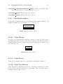
2.9.11
Class Sensor
Class Sensor inherits from Device and has the same method interface.
2.9.12
Class TouchSensor
Class TouchSensor inherits from Sensor. TouchSensor instances are used
to model the four paw touch sensors of the Aibo. These are binary sensors
returning either 0 (off) or 1 (on).
34
CHAPTER 2. SOFTWARE ARCHITECTURE
Sensor
Figure 2.23: Class Sensor
TouchSensor
Figure 2.24: Class TouchSensor
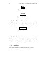
2.9.13
Class DistanceSensor
Class DistanceSensor inherits from Sensor. A DistanceSensor instance is
used to model the Position Sensing Device (PSD) of the Aibo. It returns
only positive values as measured distances cannot be negative.
DistanceSensor
Figure 2.25: Class DistanceSensor
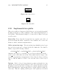
2.9.14
Class Camera
Class Camera inherits from Device. This class has not been implemented
because Aibo’s camera is not controllable via the Remote Control System4 ,
although it is in the Webots model of the Aibo. One could devote some time
to look into this issue and offer camera support in Aib-O-Matic.
2.9.15
Class LED
Class LED inherits from Device and has the same method interface.
4
See [5], section 3.5, page 30.
2.10. IMPLEMENTATION QUIRKS
35
Camera
Figure 2.26: Class Camera
LED
Figure 2.27: Class LED
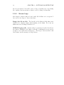
2.10
Implementation quirks
This section, while not being part of the Fondue process, is nonetheless useful.
It makes an inventory of the peculiarities of the current implementation of
Aib-O-Matic. This information might be of some value to future developers
as well as users.
Source files Every class has been put into two separate source files. A
header file Class.hh which contains the class definition and a source file
Class.cc which contains its implementation.
Of the various time steps The various time steps (simulation step, logger
step and solver step) can be adjusted in the file common.hh. Care must be
taken to respect the following condition:
SOLV ER ST EP < LOGGER ST EP < SIM U LAT ION ST EP
Otherwise the triple loop invoking solve in DynamicalSystemController ::
update systems will behave incorrectly. This results from the change of the
way the logging limitation is implemented. Before that, the NumericalSolver
used to count the number of calls to solve and sent a line of data every N
calls.
Derivate I had to choose between function pointers and methods to implement derivate in the DynamicalSystem class. I chose the latter because I
thought it would ease the task of creating lots of similar dynamical systems.
Instead this makes the equations impossible to change without creating another class. Thus the coupling, which is part of the equations, is frozen in
36
CHAPTER 2. SOFTWARE ARCHITECTURE
the derivate method. It would be nice to have a dynamic way of specifying
the coupling between systems so that it could be changed at run time.
2.10.1
Known bugs
Alas bug-free software almost doesn’t exist! Aib-O-Matic is no exception. I
discovered a few bugs too late to fix them. . .
Empty data file on Aibo The data file on the Memory Stick where state
variables are output is empty when running on the Aibo. For some yet
unknown reason, nothing is written to it.
OPEN-R logging calls System calls to log messages described in [16] are
used when compiling for the Aibo. Sadly the documentation is not precise
enough so as to where these messages go. The Logger class uses these calls
but it turns out the messages end up nowhere.
Chapter 3
Testing and results
This chapter shows the results obtained by implementing an ACPO to test
and demonstrate Aib-O-Matic. A single oscillator is used to exhibit synchronization of Aibo’s left front leg movement on the movement of its right front
leg.
3.1
Experiment setup
In order to test the software and demonstrate that it is possible to have
an online dynamical systems-based controller on the Aibo, my supervisors
and I have devised a simple experiment. One leg of the robot is controlled
by an ACPO. Another leg driven by a human user gives this oscillator a
perturbation input. If the frequency of the movement given by the user is
close enough to the intrinsic frequency of the ACPO, synchronization of the
two legs’ movement will occur. Thus demonstrating that the robot is indeed
controlled by a differential system.
The ACPO’s first state variable x will be the position of the left front
leg. The right front leg’s position will be added to ẋ multiplied by a coupling
constant k. The oscillator is specified below.
r
0
g √x2 +y2 − 1 x − yw
ẋ
+k p
=
ẏ
0
g √ r20 2 − 1 y + xw
x +y
Where:
• p is the right fore leg’s position input;
• x drives the left fore leg’s position;
37
38
CHAPTER 3. TESTING AND RESULTS
• k is the coupling constant;
• parameters:
– g = 10 is the oscillator’s gain;
– r0 = 1 is the oscillator’s radius;
– w = 2π is the oscillator’s intrinsic frequency.
Trials will be run with different values of k. According to the “Arnold
tongues” graphs (see [17]) the higher the value of k, the stronger the coupling
between the two legs will be (until a certain value of k above which it gets
chaotic).
Since this experiment consists of moving the robots legs without making it
walk, we cannot allow them to touch the ground. Otherwise their movement
will get hampered. Figures 3.1 and 3.2 show how this was accomplished in
simulation and in the real world. The Aibo lies on a box high enough to
allow its legs to move freely without touching the ground or other objects.
Figure 3.1: Experiment setup in simulation This screen
shot from Webots shows the Aibo laid on a purple rectangular
box. Such a setup allows its legs to move freely without touching
the ground or other objects.
3.2. RESULTS
39
Figure 3.2: Experiment setup in reality This photos shows
the Aibo laid on a white cardboard box. Such a setup allows its
legs to move freely without touching the ground or other objects.
3.2
Results
Here are the results I obtained while running Aib-O-Matic on a simulated
Aibo and on a real one. Movies on the project web page [18] allow you to
visualize these experiments.
3.2.1
Simulation
Webots does not yet allow the user to move parts of a robot (as opposed
to the robot as a whole). Therefore one cannot move Aibo’s right leg “by
hand”. To work around this limitation, I made the leg move with a sinusoidal
oscillation of frequency close to 2π. This movement was implement in the
robot_run controller loop in order to be outside of Aib-O-Matic.
Simulation in Webots worked pretty well apart from the robot sliding
on its supporting box after around thirty seconds causing its legs to rub
against the side of the box and disturbing measurements. Below are two
graphs of the data output by Aib-O-Matic. They show the positions of both
front legs plotted against time during the first twenty seconds of simulation.
40
CHAPTER 3. TESTING AND RESULTS
The first graph (Figure 3.3) corresponds to a run with k = 0 leading to no
synchronization. The second one (Figure 3.4) represents a run with k = 2
leading to synchronization after a few seconds. The best synchronization has
been observed with k = 2.
ACPO output and perturbation input compared, k=0
1.5
ACPO output
perturbation input
Amplitude, normalized
1
0.5
0
-0.5
-1
-1.5
0
5
10
Time [s]
15
20
Figure 3.3: ACPO and perturbation without coupling
This graph plots the ACPO output (left leg’s position) and the
perturbation input (right leg’s position) against time. Albeit the
frequencies of the two movement are close, no synchronization occurs because the coupling constant equals zero. At some points in
time (between 6–7 seconds and also between 14–15 seconds), the
two movements seem to be synchronized. Actually they aren’t
because this coincidence does not persist.
3.2.2
Reality
As in simulation, the robot has been raised on a cardboard box to allow its
legs to move freely. But this time things went bad. The legs’ movement
was erratic and jerky at best. No synchronization could be really observed.
Moreover no data could be salvaged from Aibo’s Memory Stick to explain
41
3.3. DISCUSSION
ACPO output and perturbation input compared, k=2
1.5
ACPO output
perturbation input
Amplitude, normalized
1
0.5
0
-0.5
-1
-1.5
0
5
10
Time [s]
15
20
Figure 3.4: ACPO and perturbation with coupling This
graph plots the ACPO output (left leg’s position) and the perturbation input (right leg’s position) against time. Here one can
observe a short transition period (between 0–3 seconds) before the
oscillator synchronizes on the perturbation. This synchronization
is persistent. The best synchronization has been observed with
k = 2.
this phenomenon because the data file remained mysteriously empty1 . Please
refer to the movies on the project web page [18] to see what happened.
3.3
Discussion
It turns out that simulation and real world results are radically different. This
difference is difficult to explain because no experimental data is available for
the real Aibo. Possible causes might be the differences between the simulated
Aibo model and the real one, or that the robot’s processor isn’t fast enough
to compute all derivatives in the given time step.
1
Yes, this is a bug. It is listed in section 2.10.1.
42
CHAPTER 3. TESTING AND RESULTS
Chapter 4
Conclusions
4.1
Conclusion
This project’s goal have almost been fulfilled: Webots is well integrated with
OPEN-R thanks to [4, 5], the ODE framework has been completely designed,
implemented and demonstrated. The two weaknesses remaining are that this
system really works in simulation only and needs more testing. On the other
hand, its strong points are the completeness of the software with respect to
the specification and the intrinsic documentation. We now have the tool to
test new CPGs on the Aibo.
As a whole, I enjoyed working on this project. Facing last minute hardware troubles with the Aibo and having to cope with C++’s intricacies was
compensated by the excitement of working at the boundary between strict
mathematics and animal locomotion. Using a software development method
was a bit of a masochistic initiative but it helped writing the software documentation which is of immense value to users. Speaking of users, let’s turn
to the future. . .
4.2
Future work
In decreasing order of priority here are the things to improve in Aib-O-Matic:
• Eliminate the two bugs mentioned in 2.10.1 and other yet-to-be-discovered
bugs.
• Test the software. Aib-O-Matic has only had one user yet: its author.
Real users which have no previous knowledge of the software make
much better testers.
43
44
CHAPTER 4. CONCLUSIONS
• Do some serious code refactoring to use more design patterns and to fit
the program to use with optimization methods like genetic algorithms.
• Add the feature of being able to receive data and logs via Aibo’s wireless LAN interface.
• Speed up the numerical solver or use an adaptive step method.
• Look into the library cross-compilation issue. Interesting libraries to
use include the GSL (already mentionned in section 2.9.7) for numerical
solving and GNU Nana1 for assertions checking and logging.
• Improve the Webots world file to prevent the robot from sliding on the
box.
• Add the “ultimate feature” to read differential systems’ specifications
from a file.
1
See http://www.gnu.org/software/nana/
Bibliography
[1] Webots. http://www.cyberbotics.com/. Commercial Mobile Robot
Simulation Software.
[2] J. J. Collins and S. A. Richmond. Hard-wired central pattern generators
for quadrupedal locomotion. Biological Cybernetics, 71:375–385, 1994.
[3] Jonas Buchli and Auke Jan Ijspeert. Distributed central pattern generator model for robotics application based on phase sensitivity analysis.
In A.J. Ijspeert, M. Murata, and N. Wakamiya, editors, Biologically
Inspired Approaches to Advanced Information Technology: First International Workshop, BioADIT 2004, volume 3141 of Lecture Notes in
Computer Science, pages 333–349. Springer Verlag Berlin Heidelberg,
2004.
[4] Lukas Hohl. Wireless remote control and monitoring of an AIBO robot.
Semester project, Ecole Polytechnique Fédérale de Lausanne (EPFL),
2003.
[5] Lukas Hohl. AIBO simulation in webots and controller transfer to AIBO
robot. Semester project, Ecole Polytechnique Fédérale de Lausanne
(EPFL), 2004.
[6] Mathieu Salzmann. Development of quadruped locomotion controllers
based on nonlinear oscillators. Semester project, Ecole Polytechnique
Fédérale de Lausanne (EPFL), 2003.
[7] Bertrand Mesot. Self-organisation of locomotion in modular robots.
Diploma project, Ecole Polytechnique Fédérale de Lausanne (EPFL),
2003.
[8] The Fondue Method website. http://lgl.epfl.ch/research/fondue/
index.html.
[9] Alfred Strohmeier. The Fondue Method, 2003.
45
46
BIBLIOGRAPHY
[10] Alfred Strohmeier and Shane Sendall. Operation schemas and ocl. Technical Report DI/01/358, Ecole Polytechnique Fédérale de Lausanne
(EPFL), 2001.
[11] Cyberbotics Ltd. Webots Reference Manual, 2004.
[12] Sony Corporation.
2004.
OPEN-R SDK Model Information for ERS-210,
[13] Erich Gamma, Richard Helm, Ralph Johnson, and John Vlissides. Design Patterns: Elements of Reusable Object-Oriented Software. AddisonWesley Professional Computing Series. Addison-Wesley, Boston, first
edition, October 1994.
[14] William H. Press, Brian P. Flannery, Saul A. Teukolsky, and William T.
Vetterling. Numerical Recipes in C: The Art of Scientific Computing.
Cambridge University Press, Cambridge, second edition, 1992.
[15] Rubin H. Landau and Manuel J. Pàez. Computational Physics: Problem
Solving with Computers. John Wiley & Sons, first edition, July 1997.
[16] Sony Corporation. OPEN-R SDK Programmer’s Guide, 2004.
[17] A. Pikovsky, R. Rosenblum, and J. Kurths. Synchronization, A universal concept in nonlinear sciences, volume 12 of Cambridge Nonlinear
Science Series. Cambridge University Press, Cambridge, 2001.
[18] This project’s web page. http://birg.epfl.ch/page56278.html.
[19] Sony Corporation. OPEN-R SDK Installation Guide, 2004.
Appendix A
Webots & OPEN-R Quickstart
This guide details the installation procedure on a Linux system to obtain
a running Webots with OPEN-R and RCS integration plus Aib-O-Matic
software.
A.1
OPEN-R installation
Install the OPEN-R SDK according to the instructions in [19]. These instructions are summarized below.
1. Fetch the following files from http://openr.aibo.com/ (free but registration required):
• OPEN_R_SDK-1.1.5-r3.tar.gz (OPEN-R SDK),
• OPEN_R_SDK-sample-1.1.5-r2.tar.gz (sample programs),
• OPEN_R_SDK-docE-1.1.5-r1.tar.gz (manuals),
• gcc-3.3.2.tar.gz (gcc source),
• binutils-2.14.tar.gz (binutils source),
• newlib-1.10.0.tar.gz (newlib source),
• build-devtools-3.3.2-r1.sh (installation script)
in your home directory.
2. Unpack the OPEN-R SDK:
• cd
• tar -xzf OPEN_R_SDK-1.1.5-r3.tar.gz
47
48
APPENDIX A. WEBOTS & OPEN-R QUICKSTART
This will create a new directory OPEN_R_SDK in your home directory.
3. Unpack the sample programs and documentation:
• cd OPEN_R_SDK/
• tar -xzf ../OPEN_R_SDK-sample-1.1.5-r2.tar.gz
• tar -xzf ../OPEN_R_SDK-docE-1.1.5-r1.tar.gz
• cd
4. Edit the script build-devtools-3.3.2-r1.sh to suit the installation
directory to your needs. The default is PREFIX = /usr/local/OPEN_R_
SDK. Since this guide is intended for normal (i.e. non-administrative)
users the following value will be used: PREFIX = /home/username/
OPEN_R_SDK. Replace “username” with your actual username.
5. Execute the build-devtools-3.3.2-r1.sh script. It will unpack and
compile binutils, gcc and newlib for the AIBO platform. This will take
some time. Depending on the speed of your machine, you might want
to have a drink while it is compiling. . .
A.2
Webots installation
It is assumed that Webots is already installed on your system in /usr/local/
webots. If that is not the case, head to http://www.cyberbotics.com/
products/webots/download.html and download the latest version of Webots suitable for your system or kindly ask your system administrator1 to
install it for you. Don’t forget to replace /usr/local/webots with the actual location of your Webots installation in the rest of this guide.
A.3
A.3.1
Remote Control System installation
Create your own Webots directory
• cd
• mkdir ~/my_webots
• mkdir ~/my_webots/worlds
1
Always be kind to system administrators otherwise you might dearly regret it. See
http://www.theregister.co.uk/odds/bofh/ for examples of what happens when one
isn’t.
A.3. REMOTE CONTROL SYSTEM INSTALLATION
49
• mkdir ~/my_webots/controllers
• cp /usr/local/webots/controllers/Makefile.include ~/my_webots/
controllers/
A.3.2
Extract the world file
• cd ~/my_webots/worlds/
• gunzip ~/aibo_ers210.wbt.gz
You’ll get the aibo_ers210.wbt world file in your Webots directory.
A.3.3
Install the Remote Control System
• mkdir ~/my_webots/transfer
• cd ~/my_webots/transfer/
• tar -xzf ~/openr.tgz
• mkdir ~/my_webots/src
• mkdir ~/my_webots/src/lib
• mkdir ~/my_webots/src/lib/openr
• cd ~/my_webots/src/lib/openr
• tar -xzf ~/remotecontrol.tgz
• Clean up CVS files (optional):
find . -depth -name CVS -exec rm -rv {}\;
• Delete the line #include <prototype.h> in the file ~/my_webots/
src/lib/openr/remotecontrol/Controller/Controller/Controller.
cc because prototype.h doesn’t exist anymore.
• Prepare for building:
cd ~/my_webots/src/lib/openr/remotecontrol/RCServer/
• make clean
50
APPENDIX A. WEBOTS & OPEN-R QUICKSTART
• Edit the file ~/my_webots/src/lib/openr/remotecontrol/Controller/
Controller/Makefile. Correct the values of WEBOTS_HOME and OPENRSDK_ROOT to suit your installation. That is WEBOTS_HOME should be set
to /home/username/my_webots and OPENRSDK_ROOT should be set to
/home/username/OPEN_R_SDK. Be sure to replace “username” with your
actual username.
• Run make install to build the Remote Control System.
• cd ~/my_webots/transfer/openr/remotecontrol/Controller/Controller/
• cp -v ~/my_webots/src/lib/openr/remotecontrol/Controller/Controller/
controller.* .
• cp -v ~/my_webots/src/lib/openr/remotecontrol/Controller/Controller/
Controller*.o .
• cp -v ~/my_webots/src/lib/openr/remotecontrol/Controller/Controller/
MTN*.o .
• Modify the value of WEBOTS_HOME in ~/my_webots/transfer/openr/
remotecontrol/Controller/Controller/Makefile to /home/username/
my_webots (always replacing “username” with your actual username).
• Extract files for ERS-210:
cd ~/my_webots/controllers/
• tar -xzf ~/ers210.tgz
• cd ~/my_webots/controllers/ers210/
• Modify the value of WEBOTS_HOME in ~/my_webots/controllers/ers210/
Makefile.openr to /home/username/my_webots (always replacing“username” with your actual username).
• Link to Webots installation:
cd ~/my_webots/
• ln -s /usr/local/webots/include
• ln -s /usr/local/webots/lib
A.4. AIB-O-MATIC INSTALLATION
A.4
51
Aib-O-Matic installation
• cd ~/my_webots/controllers/ers210/
• Extract Aib-O-Matic sources, be aware that this will overwrite the
Makefile.sources and Makefile files.
tar -xvzf ~/aibomatic-src.tar.gz
• Build the controller program for Webots with:
make
• Build the controller program for Aibo with:
make -f Makefile.openr
52
APPENDIX A. WEBOTS & OPEN-R QUICKSTART
Appendix B
Aib-O-Matic user manual
B.1
Installation
Follow this procedure to install Aib-O-Matic into your Webots directory. It
is assumed that this directory is ~/my_webots.
• cd ~/my_webots/controllers/ers210/
• Extract Aib-O-Matic sources, be aware that this will overwrite the
Makefile.sources and Makefile files.
tar -xvzf ~/aibomatic-src.tar.gz
B.2
How to change system parameters
Edit the file common.hh. Interesting parameters to tune include: MAX LOG LEVEL, SIMULATION STEP, LOGGER STEP and SOLVER STEP.
Care must be taken to respect the following condition:
SOLV ER ST EP < LOGGER ST EP < SIM U LAT ION ST EP
Otherwise the program will behave incorrectly.
B.3
How to build your own DynamicalSystems
First create a subclass of DynamicalSystem which overrides method derivate.
Inside this method, you can implement your own equations. You have get DS by index and get DS by name from the DynamicalSystemController at
53
54
APPENDIX B. AIB-O-MATIC USER MANUAL
your disposal to find other systems and get variable to read their variables.
Please refrain from doing anything else than reading to other DynamicalSystems, otherwise they will certainly start to behave in an unexpected manner.
Likewise, you can connect your systems with I/O devices by setting the
two boolean arrays variable to device mapping and device to variable mapping at instantiation. Use get device by index and get device by name from
the DeviceController to obtain references to devices. variable to device mapping is first indexed by variable number and then by device number.
Meaning that if the element variable_to_device_mapping[x][y] is true,
variable number x will get written to device number y after the system has
been solved. device to variable mapping is the reverse: it is indexed first by
device number and then by variable number. Meaning that if the element
device_to_variable_mapping[x][y] is true, the value of device number x
will get written to variable number y before the system is solved. You can
set those two arrays to null if you don’t use them.
Load your new systems in DynamicalSystemController ’s constructor (in
file DynamicalSystemController.cc. Add or modify array elements of array
systems. Remember to adjust the size of the array: NB DYNAMICAL SYSTEMS in common.hh. You’ll have to create all parameters before instantiating a new system. Refer to the ACPO implementation as an example (files
ACPO.hh and ACPO.cc).
B.4
How to add new Devices
You can add new devices by creating a new subclass of Device. To load
your new classes, modify the constructor in DeviceController.cc and add
new array elements to the devices array. Remember to adjust the size of the
array: NB DEVICES in common.hh.
B.5
How to compile the controller
• Build the controller program for Webots with:
make
• Build the controller program for Aibo with:
make -f Makefile.openr
Appendix C
CD-ROM table of contents
This appendix lists the contents of the CD-ROM associated with this project.
aibomatic/ Aib-O-Matic source distribution.
fondue models/ Fondue diagrams made with Dia.
images/ Screen shots and photos.
movies/ Movies of experiments.
ode out/ Sample output data files with processing scripts for GNUplot and
Matlab.
openr sdk install/ Archives files needed to install the OPEN-R SDK on
Linux.
rcs install/ Remote Control System installation files.
report/ Report LATEX source files.
slides/ Presentation slides LATEX source files.
55
56
APPENDIX C. CD-ROM TABLE OF CONTENTS
Appendix D
GNU Free Documentation
License
Version 1.2, November 2002
c
Copyright 2000,2001,2002
Free Software Foundation, Inc.
59 Temple Place, Suite 330, Boston, MA 02111-1307 USA
Everyone is permitted to copy and distribute verbatim copies of this license
document, but changing it is not allowed.
Preamble
The purpose of this License is to make a manual, textbook, or other functional
and useful document “free” in the sense of freedom: to assure everyone the
effective freedom to copy and redistribute it, with or without modifying it,
either commercially or noncommercially. Secondarily, this License preserves
for the author and publisher a way to get credit for their work, while not
being considered responsible for modifications made by others.
This License is a kind of “copyleft”, which means that derivative works
of the document must themselves be free in the same sense. It complements
the GNU General Public License, which is a copyleft license designed for free
software.
We have designed this License in order to use it for manuals for free
software, because free software needs free documentation: a free program
should come with manuals providing the same freedoms that the software
does. But this License is not limited to software manuals; it can be used
for any textual work, regardless of subject matter or whether it is published
57
58
APPENDIX D. GNU FREE DOCUMENTATION LICENSE
as a printed book. We recommend this License principally for works whose
purpose is instruction or reference.
D.1
Applicability and definitions
This License applies to any manual or other work, in any medium, that
contains a notice placed by the copyright holder saying it can be distributed
under the terms of this License. Such a notice grants a world-wide, royaltyfree license, unlimited in duration, to use that work under the conditions
stated herein. The “Document”, below, refers to any such manual or work.
Any member of the public is a licensee, and is addressed as “you”. You
accept the license if you copy, modify or distribute the work in a way requiring
permission under copyright law.
A “Modified Version” of the Document means any work containing the
Document or a portion of it, either copied verbatim, or with modifications
and/or translated into another language.
A “Secondary Section” is a named appendix or a front-matter section
of the Document that deals exclusively with the relationship of the publishers
or authors of the Document to the Document’s overall subject (or to related
matters) and contains nothing that could fall directly within that overall
subject. (Thus, if the Document is in part a textbook of mathematics, a
Secondary Section may not explain any mathematics.) The relationship could
be a matter of historical connection with the subject or with related matters,
or of legal, commercial, philosophical, ethical or political position regarding
them.
The “Invariant Sections” are certain Secondary Sections whose titles
are designated, as being those of Invariant Sections, in the notice that says
that the Document is released under this License. If a section does not fit
the above definition of Secondary then it is not allowed to be designated
as Invariant. The Document may contain zero Invariant Sections. If the
Document does not identify any Invariant Sections then there are none.
The “Cover Texts” are certain short passages of text that are listed,
as Front-Cover Texts or Back-Cover Texts, in the notice that says that the
Document is released under this License. A Front-Cover Text may be at
most 5 words, and a Back-Cover Text may be at most 25 words.
A “Transparent” copy of the Document means a machine-readable copy,
represented in a format whose specification is available to the general public,
that is suitable for revising the document straightforwardly with generic text
editors or (for images composed of pixels) generic paint programs or (for
drawings) some widely available drawing editor, and that is suitable for input
D.2. VERBATIM COPYING
59
to text formatters or for automatic translation to a variety of formats suitable
for input to text formatters. A copy made in an otherwise Transparent file
format whose markup, or absence of markup, has been arranged to thwart or
discourage subsequent modification by readers is not Transparent. An image
format is not Transparent if used for any substantial amount of text. A copy
that is not “Transparent” is called “Opaque”.
Examples of suitable formats for Transparent copies include plain ASCII
without markup, Texinfo input format, LaTeX input format, SGML or XML
using a publicly available DTD, and standard-conforming simple HTML,
PostScript or PDF designed for human modification. Examples of transparent image formats include PNG, XCF and JPG. Opaque formats include
proprietary formats that can be read and edited only by proprietary word
processors, SGML or XML for which the DTD and/or processing tools are
not generally available, and the machine-generated HTML, PostScript or
PDF produced by some word processors for output purposes only.
The “Title Page” means, for a printed book, the title page itself, plus
such following pages as are needed to hold, legibly, the material this License
requires to appear in the title page. For works in formats which do not have
any title page as such, “Title Page” means the text near the most prominent
appearance of the work’s title, preceding the beginning of the body of the
text.
A section “Entitled XYZ” means a named subunit of the Document
whose title either is precisely XYZ or contains XYZ in parentheses following text that translates XYZ in another language. (Here XYZ stands for
a specific section name mentioned below, such as “Acknowledgements”,
“Dedications”, “Endorsements”, or “History”.) To “Preserve the Title” of such a section when you modify the Document means that it remains
a section “Entitled XYZ” according to this definition.
The Document may include Warranty Disclaimers next to the notice
which states that this License applies to the Document. These Warranty
Disclaimers are considered to be included by reference in this License, but
only as regards disclaiming warranties: any other implication that these Warranty Disclaimers may have is void and has no effect on the meaning of this
License.
D.2
Verbatim copying
You may copy and distribute the Document in any medium, either commercially or noncommercially, provided that this License, the copyright notices,
and the license notice saying this License applies to the Document are re-
60
APPENDIX D. GNU FREE DOCUMENTATION LICENSE
produced in all copies, and that you add no other conditions whatsoever to
those of this License. You may not use technical measures to obstruct or
control the reading or further copying of the copies you make or distribute.
However, you may accept compensation in exchange for copies. If you distribute a large enough number of copies you must also follow the conditions
in section 3.
You may also lend copies, under the same conditions stated above, and
you may publicly display copies.
D.3
Copying in quantity
If you publish printed copies (or copies in media that commonly have printed
covers) of the Document, numbering more than 100, and the Document’s
license notice requires Cover Texts, you must enclose the copies in covers
that carry, clearly and legibly, all these Cover Texts: Front-Cover Texts on
the front cover, and Back-Cover Texts on the back cover. Both covers must
also clearly and legibly identify you as the publisher of these copies. The front
cover must present the full title with all words of the title equally prominent
and visible. You may add other material on the covers in addition. Copying
with changes limited to the covers, as long as they preserve the title of the
Document and satisfy these conditions, can be treated as verbatim copying
in other respects.
If the required texts for either cover are too voluminous to fit legibly,
you should put the first ones listed (as many as fit reasonably) on the actual
cover, and continue the rest onto adjacent pages.
If you publish or distribute Opaque copies of the Document numbering more than 100, you must either include a machine-readable Transparent
copy along with each Opaque copy, or state in or with each Opaque copy
a computer-network location from which the general network-using public
has access to download using public-standard network protocols a complete
Transparent copy of the Document, free of added material. If you use the
latter option, you must take reasonably prudent steps, when you begin distribution of Opaque copies in quantity, to ensure that this Transparent copy
will remain thus accessible at the stated location until at least one year after
the last time you distribute an Opaque copy (directly or through your agents
or retailers) of that edition to the public.
It is requested, but not required, that you contact the authors of the
Document well before redistributing any large number of copies, to give them
a chance to provide you with an updated version of the Document.
D.4. MODIFICATIONS
D.4
61
Modifications
You may copy and distribute a Modified Version of the Document under the
conditions of sections 2 and 3 above, provided that you release the Modified
Version under precisely this License, with the Modified Version filling the role
of the Document, thus licensing distribution and modification of the Modified
Version to whoever possesses a copy of it. In addition, you must do these
things in the Modified Version:
A. Use in the Title Page (and on the covers, if any) a title distinct from that
of the Document, and from those of previous versions (which should, if
there were any, be listed in the History section of the Document). You
may use the same title as a previous version if the original publisher of
that version gives permission.
B. List on the Title Page, as authors, one or more persons or entities responsible for authorship of the modifications in the Modified Version, together
with at least five of the principal authors of the Document (all of its principal authors, if it has fewer than five), unless they release you from this
requirement.
C. State on the Title page the name of the publisher of the Modified Version,
as the publisher.
D. Preserve all the copyright notices of the Document.
E. Add an appropriate copyright notice for your modifications adjacent to
the other copyright notices.
F. Include, immediately after the copyright notices, a license notice giving
the public permission to use the Modified Version under the terms of this
License, in the form shown in the Addendum below.
G. Preserve in that license notice the full lists of Invariant Sections and
required Cover Texts given in the Document’s license notice.
H. Include an unaltered copy of this License.
I. Preserve the section Entitled “History”, Preserve its Title, and add to
it an item stating at least the title, year, new authors, and publisher of
the Modified Version as given on the Title Page. If there is no section
Entitled “History” in the Document, create one stating the title, year,
authors, and publisher of the Document as given on its Title Page, then
add an item describing the Modified Version as stated in the previous
sentence.
62
APPENDIX D. GNU FREE DOCUMENTATION LICENSE
J. Preserve the network location, if any, given in the Document for public
access to a Transparent copy of the Document, and likewise the network
locations given in the Document for previous versions it was based on.
These may be placed in the “History” section. You may omit a network
location for a work that was published at least four years before the
Document itself, or if the original publisher of the version it refers to
gives permission.
K. For any section Entitled “Acknowledgements” or “Dedications”, Preserve
the Title of the section, and preserve in the section all the substance
and tone of each of the contributor acknowledgements and/or dedications
given therein.
L. Preserve all the Invariant Sections of the Document, unaltered in their
text and in their titles. Section numbers or the equivalent are not considered part of the section titles.
M. Delete any section Entitled “Endorsements”. Such a section may not be
included in the Modified Version.
N. Do not retitle any existing section to be Entitled “Endorsements” or to
conflict in title with any Invariant Section.
O. Preserve any Warranty Disclaimers.
If the Modified Version includes new front-matter sections or appendices
that qualify as Secondary Sections and contain no material copied from the
Document, you may at your option designate some or all of these sections
as invariant. To do this, add their titles to the list of Invariant Sections in
the Modified Version’s license notice. These titles must be distinct from any
other section titles.
You may add a section Entitled “Endorsements”, provided it contains
nothing but endorsements of your Modified Version by various parties–for
example, statements of peer review or that the text has been approved by an
organization as the authoritative definition of a standard.
You may add a passage of up to five words as a Front-Cover Text, and a
passage of up to 25 words as a Back-Cover Text, to the end of the list of Cover
Texts in the Modified Version. Only one passage of Front-Cover Text and
one of Back-Cover Text may be added by (or through arrangements made
by) any one entity. If the Document already includes a cover text for the
same cover, previously added by you or by arrangement made by the same
entity you are acting on behalf of, you may not add another; but you may
D.5. COMBINING DOCUMENTS
63
replace the old one, on explicit permission from the previous publisher that
added the old one.
The author(s) and publisher(s) of the Document do not by this License
give permission to use their names for publicity for or to assert or imply
endorsement of any Modified Version.
D.5
Combining documents
You may combine the Document with other documents released under this
License, under the terms defined in section 4 above for modified versions,
provided that you include in the combination all of the Invariant Sections
of all of the original documents, unmodified, and list them all as Invariant
Sections of your combined work in its license notice, and that you preserve
all their Warranty Disclaimers.
The combined work need only contain one copy of this License, and multiple identical Invariant Sections may be replaced with a single copy. If there
are multiple Invariant Sections with the same name but different contents,
make the title of each such section unique by adding at the end of it, in
parentheses, the name of the original author or publisher of that section if
known, or else a unique number. Make the same adjustment to the section
titles in the list of Invariant Sections in the license notice of the combined
work.
In the combination, you must combine any sections Entitled “History”
in the various original documents, forming one section Entitled “History”;
likewise combine any sections Entitled “Acknowledgements”, and any sections
Entitled“Dedications”. You must delete all sections Entitled“Endorsements”.
D.6
Collections of documents
You may make a collection consisting of the Document and other documents
released under this License, and replace the individual copies of this License
in the various documents with a single copy that is included in the collection,
provided that you follow the rules of this License for verbatim copying of each
of the documents in all other respects.
You may extract a single document from such a collection, and distribute
it individually under this License, provided you insert a copy of this License
into the extracted document, and follow this License in all other respects
regarding verbatim copying of that document.
64
D.7
APPENDIX D. GNU FREE DOCUMENTATION LICENSE
Aggregation with independent works
A compilation of the Document or its derivatives with other separate and
independent documents or works, in or on a volume of a storage or distribution medium, is called an “aggregate” if the copyright resulting from the
compilation is not used to limit the legal rights of the compilation’s users beyond what the individual works permit. When the Document is included in
an aggregate, this License does not apply to the other works in the aggregate
which are not themselves derivative works of the Document.
If the Cover Text requirement of section 3 is applicable to these copies
of the Document, then if the Document is less than one half of the entire
aggregate, the Document’s Cover Texts may be placed on covers that bracket
the Document within the aggregate, or the electronic equivalent of covers if
the Document is in electronic form. Otherwise they must appear on printed
covers that bracket the whole aggregate.
D.8
Translation
Translation is considered a kind of modification, so you may distribute translations of the Document under the terms of section 4. Replacing Invariant
Sections with translations requires special permission from their copyright
holders, but you may include translations of some or all Invariant Sections in
addition to the original versions of these Invariant Sections. You may include
a translation of this License, and all the license notices in the Document, and
any Warranty Disclaimers, provided that you also include the original English version of this License and the original versions of those notices and
disclaimers. In case of a disagreement between the translation and the original version of this License or a notice or disclaimer, the original version will
prevail.
If a section in the Document is Entitled “Acknowledgements”, “Dedications”, or “History”, the requirement (section 4) to Preserve its Title (section
1) will typically require changing the actual title.
D.9
Termination
You may not copy, modify, sublicense, or distribute the Document except
as expressly provided for under this License. Any other attempt to copy,
modify, sublicense or distribute the Document is void, and will automatically
terminate your rights under this License. However, parties who have received
D.10. FUTURE REVISIONS OF THIS LICENSE
65
copies, or rights, from you under this License will not have their licenses
terminated so long as such parties remain in full compliance.
D.10
Future revisions of this license
The Free Software Foundation may publish new, revised versions of the GNU
Free Documentation License from time to time. Such new versions will be
similar in spirit to the present version, but may differ in detail to address
new problems or concerns. See http://www.gnu.org/copyleft/.
Each version of the License is given a distinguishing version number. If
the Document specifies that a particular numbered version of this License “or
any later version” applies to it, you have the option of following the terms
and conditions either of that specified version or of any later version that
has been published (not as a draft) by the Free Software Foundation. If the
Document does not specify a version number of this License, you may choose
any version ever published (not as a draft) by the Free Software Foundation.
Addendum: How to use this License for your
documents
To use this License in a document you have written, include a copy of the
License in the document and put the following copyright and license notices
just after the title page:
c
Copyright YEAR
YOUR NAME. Permission is granted to copy,
distribute and/or modify this document under the terms of the
GNU Free Documentation License, Version 1.2 or any later version published by the Free Software Foundation; with no Invariant Sections, no Front-Cover Texts, and no Back-Cover Texts. A
copy of the license is included in the section entitled “GNU Free
Documentation License”.
If you have Invariant Sections, Front-Cover Texts and Back-Cover Texts,
replace the “with. . . Texts.” line with this:
with the Invariant Sections being LIST THEIR TITLES, with the
Front-Cover Texts being LIST, and with the Back-Cover Texts
being LIST.
66
APPENDIX D. GNU FREE DOCUMENTATION LICENSE
If you have Invariant Sections without Cover Texts, or some other combination of the three, merge those two alternatives to suit the situation.
If your document contains nontrivial examples of program code, we recommend releasing these examples in parallel under your choice of free software
license, such as the GNU General Public License, to permit their use in free
software.
Appendix E
GNU General Public License
Version 2, June 1991
c 1989, 1991 Free Software Foundation, Inc.
Copyright 59 Temple Place - Suite 330, Boston, MA 02111-1307, USA
Everyone is permitted to copy and distribute verbatim copies of this license
document, but changing it is not allowed.
Preamble
The licenses for most software are designed to take away your freedom to
share and change it. By contrast, the GNU General Public License is intended
to guarantee your freedom to share and change free software—to make sure
the software is free for all its users. This General Public License applies to
most of the Free Software Foundation’s software and to any other program
whose authors commit to using it. (Some other Free Software Foundation
software is covered by the GNU Library General Public License instead.)
You can apply it to your programs, too.
When we speak of free software, we are referring to freedom, not price.
Our General Public Licenses are designed to make sure that you have the
freedom to distribute copies of free software (and charge for this service if
you wish), that you receive source code or can get it if you want it, that you
can change the software or use pieces of it in new free programs; and that
you know you can do these things.
To protect your rights, we need to make restrictions that forbid anyone to
deny you these rights or to ask you to surrender the rights. These restrictions
translate to certain responsibilities for you if you distribute copies of the
software, or if you modify it.
67
68
APPENDIX E. GNU GENERAL PUBLIC LICENSE
For example, if you distribute copies of such a program, whether gratis
or for a fee, you must give the recipients all the rights that you have. You
must make sure that they, too, receive or can get the source code. And you
must show them these terms so they know their rights.
We protect your rights with two steps: (1) copyright the software, and
(2) offer you this license which gives you legal permission to copy, distribute
and/or modify the software.
Also, for each author’s protection and ours, we want to make certain that
everyone understands that there is no warranty for this free software. If the
software is modified by someone else and passed on, we want its recipients to
know that what they have is not the original, so that any problems introduced
by others will not reflect on the original authors’ reputations.
Finally, any free program is threatened constantly by software patents.
We wish to avoid the danger that redistributors of a free program will individually obtain patent licenses, in effect making the program proprietary.
To prevent this, we have made it clear that any patent must be licensed for
everyone’s free use or not licensed at all.
The precise terms and conditions for copying, distribution and modification follow.
Terms and Conditions For Copying, Distribution and Modification
0. This License applies to any program or other work which contains a
notice placed by the copyright holder saying it may be distributed under the terms of this General Public License. The “Program”, below,
refers to any such program or work, and a “work based on the Program”
means either the Program or any derivative work under copyright law:
that is to say, a work containing the Program or a portion of it, either verbatim or with modifications and/or translated into another
language. (Hereinafter, translation is included without limitation in
the term “modification”.) Each licensee is addressed as “you”.
Activities other than copying, distribution and modification are not
covered by this License; they are outside its scope. The act of running
the Program is not restricted, and the output from the Program is
covered only if its contents constitute a work based on the Program
(independent of having been made by running the Program). Whether
that is true depends on what the Program does.
1. You may copy and distribute verbatim copies of the Program’s source
69
code as you receive it, in any medium, provided that you conspicuously
and appropriately publish on each copy an appropriate copyright notice
and disclaimer of warranty; keep intact all the notices that refer to
this License and to the absence of any warranty; and give any other
recipients of the Program a copy of this License along with the Program.
You may charge a fee for the physical act of transferring a copy, and
you may at your option offer warranty protection in exchange for a fee.
2. You may modify your copy or copies of the Program or any portion of
it, thus forming a work based on the Program, and copy and distribute
such modifications or work under the terms of Section 1 above, provided
that you also meet all of these conditions:
(a) You must cause the modified files to carry prominent notices stating that you changed the files and the date of any change.
(b) You must cause any work that you distribute or publish, that in
whole or in part contains or is derived from the Program or any
part thereof, to be licensed as a whole at no charge to all third
parties under the terms of this License.
(c) If the modified program normally reads commands interactively
when run, you must cause it, when started running for such interactive use in the most ordinary way, to print or display an
announcement including an appropriate copyright notice and a
notice that there is no warranty (or else, saying that you provide
a warranty) and that users may redistribute the program under
these conditions, and telling the user how to view a copy of this
License. (Exception: if the Program itself is interactive but does
not normally print such an announcement, your work based on
the Program is not required to print an announcement.)
These requirements apply to the modified work as a whole. If identifiable sections of that work are not derived from the Program, and
can be reasonably considered independent and separate works in themselves, then this License, and its terms, do not apply to those sections
when you distribute them as separate works. But when you distribute
the same sections as part of a whole which is a work based on the
Program, the distribution of the whole must be on the terms of this License, whose permissions for other licensees extend to the entire whole,
and thus to each and every part regardless of who wrote it.
Thus, it is not the intent of this section to claim rights or contest your
rights to work written entirely by you; rather, the intent is to exercise
70
APPENDIX E. GNU GENERAL PUBLIC LICENSE
the right to control the distribution of derivative or collective works
based on the Program.
In addition, mere aggregation of another work not based on the Program with the Program (or with a work based on the Program) on a
volume of a storage or distribution medium does not bring the other
work under the scope of this License.
3. You may copy and distribute the Program (or a work based on it, under
Section 2) in object code or executable form under the terms of Sections
1 and 2 above provided that you also do one of the following:
(a) Accompany it with the complete corresponding machine-readable
source code, which must be distributed under the terms of Sections 1 and 2 above on a medium customarily used for software
interchange; or,
(b) Accompany it with a written offer, valid for at least three years, to
give any third party, for a charge no more than your cost of physically performing source distribution, a complete machine-readable
copy of the corresponding source code, to be distributed under the
terms of Sections 1 and 2 above on a medium customarily used
for software interchange; or,
(c) Accompany it with the information you received as to the offer to
distribute corresponding source code. (This alternative is allowed
only for noncommercial distribution and only if you received the
program in object code or executable form with such an offer, in
accord with Subsection b above.)
The source code for a work means the preferred form of the work for
making modifications to it. For an executable work, complete source
code means all the source code for all modules it contains, plus any associated interface definition files, plus the scripts used to control compilation and installation of the executable. However, as a special exception, the source code distributed need not include anything that is
normally distributed (in either source or binary form) with the major
components (compiler, kernel, and so on) of the operating system on
which the executable runs, unless that component itself accompanies
the executable.
If distribution of executable or object code is made by offering access
to copy from a designated place, then offering equivalent access to copy
the source code from the same place counts as distribution of the source
71
code, even though third parties are not compelled to copy the source
along with the object code.
4. You may not copy, modify, sublicense, or distribute the Program except as expressly provided under this License. Any attempt otherwise
to copy, modify, sublicense or distribute the Program is void, and will
automatically terminate your rights under this License. However, parties who have received copies, or rights, from you under this License
will not have their licenses terminated so long as such parties remain
in full compliance.
5. You are not required to accept this License, since you have not signed it.
However, nothing else grants you permission to modify or distribute the
Program or its derivative works. These actions are prohibited by law if
you do not accept this License. Therefore, by modifying or distributing
the Program (or any work based on the Program), you indicate your
acceptance of this License to do so, and all its terms and conditions for
copying, distributing or modifying the Program or works based on it.
6. Each time you redistribute the Program (or any work based on the
Program), the recipient automatically receives a license from the original licensor to copy, distribute or modify the Program subject to these
terms and conditions. You may not impose any further restrictions
on the recipients’ exercise of the rights granted herein. You are not
responsible for enforcing compliance by third parties to this License.
7. If, as a consequence of a court judgment or allegation of patent infringement or for any other reason (not limited to patent issues), conditions
are imposed on you (whether by court order, agreement or otherwise)
that contradict the conditions of this License, they do not excuse you
from the conditions of this License. If you cannot distribute so as
to satisfy simultaneously your obligations under this License and any
other pertinent obligations, then as a consequence you may not distribute the Program at all. For example, if a patent license would not
permit royalty-free redistribution of the Program by all those who receive copies directly or indirectly through you, then the only way you
could satisfy both it and this License would be to refrain entirely from
distribution of the Program.
If any portion of this section is held invalid or unenforceable under any
particular circumstance, the balance of the section is intended to apply
and the section as a whole is intended to apply in other circumstances.
72
APPENDIX E. GNU GENERAL PUBLIC LICENSE
It is not the purpose of this section to induce you to infringe any patents
or other property right claims or to contest validity of any such claims;
this section has the sole purpose of protecting the integrity of the free
software distribution system, which is implemented by public license
practices. Many people have made generous contributions to the wide
range of software distributed through that system in reliance on consistent application of that system; it is up to the author/donor to decide
if he or she is willing to distribute software through any other system
and a licensee cannot impose that choice.
This section is intended to make thoroughly clear what is believed to
be a consequence of the rest of this License.
8. If the distribution and/or use of the Program is restricted in certain
countries either by patents or by copyrighted interfaces, the original
copyright holder who places the Program under this License may add an
explicit geographical distribution limitation excluding those countries,
so that distribution is permitted only in or among countries not thus
excluded. In such case, this License incorporates the limitation as if
written in the body of this License.
9. The Free Software Foundation may publish revised and/or new versions
of the General Public License from time to time. Such new versions
will be similar in spirit to the present version, but may differ in detail
to address new problems or concerns.
Each version is given a distinguishing version number. If the Program
specifies a version number of this License which applies to it and “any
later version”, you have the option of following the terms and conditions
either of that version or of any later version published by the Free
Software Foundation. If the Program does not specify a version number
of this License, you may choose any version ever published by the Free
Software Foundation.
10. If you wish to incorporate parts of the Program into other free programs
whose distribution conditions are different, write to the author to ask
for permission. For software which is copyrighted by the Free Software
Foundation, write to the Free Software Foundation; we sometimes make
exceptions for this. Our decision will be guided by the two goals of
preserving the free status of all derivatives of our free software and of
promoting the sharing and reuse of software generally.
No Warranty
73
11. Because the program is licensed free of charge, there is
no warranty for the program, to the extent permitted
by applicable law. Except when otherwise stated in writing the copyright holders and/or other parties provide
the program “as is” without warranty of any kind, either
expressed or implied, including, but not limited to, the
implied warranties of merchantability and fitness for a
particular purpose. The entire risk as to the quality and
performance of the program is with you. Should the program prove defective, you assume the cost of all necessary servicing, repair or correction.
12. In no event unless required by applicable law or agreed
to in writing will any copyright holder, or any other
party who may modify and/or redistribute the program as
permitted above, be liable to you for damages, including
any general, special, incidental or consequential damages
arising out of the use or inability to use the program
(including but not limited to loss of data or data being
rendered inaccurate or losses sustained by you or third
parties or a failure of the program to operate with any
other programs), even if such holder or other party has
been advised of the possibility of such damages.
End of Terms and Conditions
Appendix: How to Apply These Terms to Your
New Programs
If you develop a new program, and you want it to be of the greatest possible
use to the public, the best way to achieve this is to make it free software
which everyone can redistribute and change under these terms.
To do so, attach the following notices to the program. It is safest to
attach them to the start of each source file to most effectively convey the
exclusion of warranty; and each file should have at least the “copyright” line
and a pointer to where the full notice is found.
one line to give the program’s name and a brief idea of what it
does.
Copyright (C) yyyy name of author
74
APPENDIX E. GNU GENERAL PUBLIC LICENSE
This program is free software; you can redistribute it and/or modify it under the terms of the GNU General Public License as published by the Free Software Foundation; either version 2 of the
License, or (at your option) any later version.
This program is distributed in the hope that it will be useful,
but WITHOUT ANY WARRANTY; without even the implied
warranty of MERCHANTABILITY or FITNESS FOR A PARTICULAR PURPOSE. See the GNU General Public License for
more details.
You should have received a copy of the GNU General Public License along with this program; if not, write to the Free Software
Foundation, Inc., 59 Temple Place - Suite 330, Boston, MA 021111307, USA.
Also add information on how to contact you by electronic and paper mail.
If the program is interactive, make it output a short notice like this when
it starts in an interactive mode:
Gnomovision version 69, Copyright (C) yyyy name of author
Gnomovision comes with ABSOLUTELY NO WARRANTY; for
details type ‘show w’.
This is free software, and you are welcome to redistribute it under
certain conditions; type ‘show c’ for details.
The hypothetical commands show w and show c should show the appropriate parts of the General Public License. Of course, the commands you use
may be called something other than show w and show c; they could even be
mouse-clicks or menu items—whatever suits your program.
You should also get your employer (if you work as a programmer) or your
school, if any, to sign a “copyright disclaimer” for the program, if necessary.
Here is a sample; alter the names:
Yoyodyne, Inc., hereby disclaims all copyright interest in the program
‘Gnomovision’ (which makes passes at compilers) written by James
Hacker.
signature of Ty Coon, 1 April 1989
Ty Coon, President of Vice
75
This General Public License does not permit incorporating your program
into proprietary programs. If your program is a subroutine library, you may
consider it more useful to permit linking proprietary applications with the
library. If this is what you want to do, use the GNU Library General Public
License instead of this License.
76
APPENDIX E. GNU GENERAL PUBLIC LICENSE