Download Automation of Optical Test Equipment using LabVIEW

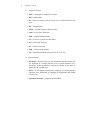
A U T O M AT I O N O F O P T I C A L T E S T E Q U I P M E N T U S I N G
LABVIEW
matteo rampado
– Aprile 2014–
Matteo Rampado: Automation of Optical Test Equipment using LabVIEW,
Corso di Laurea Magistrale in Ingegneria dell’Automazione, Dipartimento di Ingegneria dell’Informazione, Padova, © Aprile 2014
Università degli Studi di Padova
Dipartimento di Ingegneria dell’Informazione
____
University of Glasgow
____
Corso di Laurea Magistrale in Ingegneria dell’Automazione
Tesi di Laurea
Automation of Optical Test Equipment
using LabVIEW
Candidato: Matteo Rampado
Relatore di Glasgow: Dr. Anthony Kelly
Relatore di Padova: Dott. Luca Palmieri
Anno Accademico 2013-2014
ABSTRACT
A blue array of GaN-based µLEDs and a Golden Dragon Plus commercial LED (OSRAM) were analysed under a pulsed current. A
LabVIEW program by National InstrumentsTM is used to automate
the measurements of the envelope at the top of the pulse at different
frequencies. The program allows to save, to plot and to elaborate the
data measured. The results, characterised by noise at high frequencies, show an increase of the bandwidth with the voltage of the pulse
applied. In the array of µLEDs the bandwidth increases using smaller
pixels. However these pixels can carry a limited voltage. On the other
side, the commercial LED carries high voltages but is limited in bandwidth due to its internal properties. Finally, pulse conditions improve
the performance of the µLED. In respect to a pulse, a DC current sent
to the µLED leads to lower bandwidths. The first part of the report
presents the experiments and the results. A manual for the LabVIEW
programs used is given in the second and last part.
v
ACKNOWLEDGMENTS
I would like to acknowledge the assistance that the following individuals gave to me throughout the project.
To my supervisor Dr. Anthony Kelly, who assisted me well during
the work of these months, even in the most busy moments.
To Scott Watson, who spent a lot of time with me in the lab and
who gave me the best help possible with the equipment and the experiments.
vii
to my family and to Valentina
ix
CONTENTS
i indroduction
1 introduction
1.1 Abbreviations
1.2 Definitions
1
3
4
4
ii chapters
5
2 experiments
7
2.1 LED: measure of the envelope using the pulse
7
2.1.1 Setup for the measurement
8
2.1.2 Different configurations: the insertion of attenuators
9
2.1.3 Calibration
11
2.1.4 Error in the measurements and data elaboration
14
2.1.5 µLED, Results
15
2.1.6 Commercial LED, Results
20
2.2 µLED, measure of the envelope with DC current
22
3 remote control
27
3.1 Connections
27
3.2 Front Panel
27
3.2.1 LOG IN
27
3.2.2 RUN
29
3.2.3 CONFIGURE
31
3.2.4 RESULTS
35
4 programming
37
4.1 General advices about the programs
37
4.2 Configuration
38
4.2.1 Pulse Generator
38
4.2.2 Oscilloscope
38
4.2.3 Network Analyzer
41
4.3 Visualisation
41
4.4 Measurements
44
4.5 Data Save
48
4.6 Data elaboration
48
4.7 State-machine concept and MainProgram.vi
53
iii conclusions
55
5 conclusions
57
5.1 Experiments
57
5.2 Programming
57
6 future work
59
xi
xii
contents
iv appendix
61
a labview tools
63
a.1 About LabVIEW
63
a.2 Typical functionalities used
Bibliography
66
64
LIST OF FIGURES
Figure 1
Figure 2
Figure 3
Figure 4
Figure 5
Figure 6
Figure 7
Figure 8
Figure 9
Figure 10
Figure 11
Figure 12
Figure 13
Figure 14
Figure 15
Figure 16
Figure 17
Figure 18
Figure 19
Figure 20
Figure 21
Figure 22
Figure 23
Figure 24
Figure 25
Figure 26
Figure 27
Connections for the measure of the envelope
using the pulse
8
Solution used in case of no-flat waves displayed
by the oscilloscope
9
Envelope in dB versus Frequency in MHz, pixel
40µm, 5 V
10
Connections for Calibration
11
Calibration, 5 V and 1% Duty Cycle.
12
Calibration, 5 V and 1% Duty Cycle.
13
Comparison Voltages and µLEDs
16
Comparison Voltages and µLEDs
17
Comparison Voltages and µLEDs
18
Bandwidth function of the voltage for all the
µLEDs
19
Envelope vs frequency for different Duty Cycles, 5 V, 3rd µLED (50µm) first row.
19
BW versus Voltage for the Commercial LED,
DF = 250 MHz, raw values
21
Comparison Voltages for the Commercial LED,
DF = 50 MHz
21
BW versus Voltage for the Commercial LED,
DF = 50 MHz
22
Connections for the measure of the envelope
with DC current
22
Envelope function of the frequency at different
voltages for pulsed (1% duty cycle) and direct
current conditions
24
Comparison of the bandwidths for pulsed (1%
duty cycle) and direct current conditions
25
MainProgram.vi, front panel
28
LogIn.vi, front panel
28
Run.vi, front panel
29
Run.vi, front panel, tab NA
30
Results.vi, front panel
31
Configuration.vi, front panel
32
Configuration.vi, front panel, tab with the controls for the PG
33
Configuration.vi, front panel, tab with the controls for the oscilloscope
34
Configuration for the Pulse Generator
38
Configuration for the Oscilloscope
39
xiii
xiv
List of Figures
Figure 28
Figure 29
Figure 30
Figure 31
Figure 32
Figure 33
Figure 34
Figure 35
Figure 36
Figure 37
Figure 38
Figure 39
Figure 40
Figure 41
Figure 42
Figure 43
Figure 44
Configuration for the acquisition of the oscilloscope
40
Configuration for the horizontal axis in the display of the oscilloscope
41
Configuration for the Network Analyzer
42
Part of the block diagram of Configuration.vi,
controls and real-time illustration of the configuration used
43
rss_vscaleGraph.vi Block Diagram, generation of
a waveform with maximum and minimum values of the display of the Oscilloscope
44
Measure of the envelope and of the minimum
voltage
45
Low function, envelope in dB and data calibration
45
Calculation of the calibration factors
46
Part of the code of Run.vi
47
Envelope saving
49
Save into Spreadsheet file
50
Code for saving the graphs
50
Block diagram for the elaboration of the data:
normalisation, fit, interpolation and BW calculation
52
State machine for the main program
53
Block diagram of the main program
53
Some structures of LabVIEW
64
Example of the use of the Shift Register
65
Part I
INDRODUCTION
1
INTRODUCTION
Directly from the title, Optical and Automation are the key words of
this project. Optical is related to the equipment used; Automation is
represented by the use of LabVIEW. They include the two main aims,
to find the bandwidth of some devices and to design a program for
the control of the equipment.
Two different LEDs are analysed, a blue array of GaN-based µLEDs
made by the institute of photonics (University of Strathclyde) and a
Golden Dragon Plus commercial LED (OSRAM). The array of µLEDs
is a square of 16 × 16 pixels. In each row there are, from left to right
and in the form number × diameter, 2 × 5µm - 2 × 10µm - 2 × 15µm
- 2 × 20µm - 2 × 30µm - 2 × 40µm - 2 × 50µm - 2 × 60µm pixels. The
commercial LED has a diameter of 1mm2 . Firstly, the LEDs are subjected to pulse conditions. The part of interest is the top of the pulse
sent, the interval of time when the LED is ON. In this interval the
envelope measure is taken at different frequencies, to find the bandwidth of the LED. In this report the electrical bandwidth is considered, such the frequency at which the envelope is reduced by 3 dB
compared with its measure at the initial frequency. The experiments
are repeated changing some parameters of the pulse, as the voltage
and the duty cycle. Finally, only for the µLEDs, the experiment is repeated under continuous current. The second chapter describes the
optical equipment and the experiments done, showing results and
their elaboration.
Automated systems are becoming more and more important in the
technological development. Computer programs facilitate the work
of engineers and designers, allowing to save time especially for repetitive measurements, as in this case. So the best way to do the measurements for the calculation of the bandwidth is to control the instruments automatically. LabVIEW presents two main environments
strictly connected each other. The Front Panel is the user’s interface,
formed by controls and indicators which allow the user to control
the instruments and to have access to the results. It is presented in
the third chapter, together with the connections laptop-instruments.
The Block Diagram is the code of the program, in the form of graphical programming. It contains icons representing either functions or
subprograms. The code is investigated in the fourth chapter. For the
reader new to LabVIEW, Appendix A offers a brief description of
some features used in the program.
The Abbreviations and Definitions present throughout the report
are given below.
3
4
introduction
1.1
abbreviations
• ADC = Analogue to Digital Converter
• BW = Bandwidth
• DC = Direct Current or Duty Cycle (it is evident from the context)
• DF = Digital Filter
• GPIB = General Purpose Interface Bus
• LAN = Local Area Network
• LED = Light Emitting Diode
• LP = Low Pass (referred to the filter)
• NA = Network Analyzer
• PG = Pulse Generator
• USB = Universal Serial Bus
• VI = Virtual Instrument (also present as vi or .vi)
1.2
definitions
• Envelope = distance between the minimum and maximum values detected in a sample interval over a certain number of acquisitions. In this report this concept is referred to the data acquired by the oscilloscope.
• Pulse = in the Signal and Systems language it is a Rectangular
function, here translated or changed in amplitude and width
case by case.
• Virtual Instrument = program of LabVIEW.
Part II
CHAPTERS
2
EXPERIMENTS
All the project revolves around two kinds of Light Emitting Diode
(LED), a blue array of GaN-based µLEDs and a Golden Dragon Plus
commercial LED. As indicated in the Introduction, the array of µLEDs
is provided by the Institute of Photonics of the University of Strathclyde, whereas the Golden Drangon Plus LED is given by OSRAM.
The analysis is divided into two main sections, which differ from the
current at the input of the LEDs. This is respectively pulsed and continuous for the first and the second section.
Both the experiments focus on the calculation of the bandwidth
of the devices under different conditions. This is done through the
measure of the envelope on the output signal of the LEDs at different
frequencies. Furthermore, the envelope is expected to be steady at
low frequencies and to roll off quickly at high frequencies.
The instruments used for the experiments and their functions, by
which they are used for, are listed below.
1. Pulse Generator, HW 8114A - to analyse the LEDs under pulse
conditions.
2. Network Analyzer, HP 8753ES - to analyse the LEDs at different
frequencies.
3. Ultra High Speed Photoreceiver HSA-X-S-1G4-SI, made by the
company FEMTO Messtechnik GmbH (called also Detector in
this report) - to detect the optical signal generated by the LED
and to convert this signal into its electrical form.
4. Oscilloscope, Rohde & Schawarz RTO1022 - to show the data
generated by the Photoreceiver, to make measurements and save
the results.
5. DC current supply, Thurlby-Thandar PL 310QMD - to analyse
the LEDs under continuous current.
6. Digital Multimeter, Keithley 195A - to improve the source of
continuous current to the order of mA.
2.1
led: measure of the envelope using the pulse
For this experiment the instruments 1 − 4 are used, connected as in
Figure 1. A pulse is generated from the PG and goes inside a T-splitter,
where the NA and the LED are connected. In case of the µLED the
signal goes through a probe connected to the pixel analysed. On the
7
8
experiments
Figure 1: Connections for the measure of the envelope using the pulse
other hand the signal goes directly to the commercial LED. The light
of the LED is detected and converted into an electrical signal by the
Photoreceiver. This last signal goes to the oscilloscope where it is
analysed.
2.1.1
Setup for the measurement
Firstly, the PG is set for a pulse with a period of 100 µs and a duty
cycle of 1% (1 µs of pulse width). Furthermore, the NA is set to sweep
frequency from an input list in the interval 1 MHz-1 GHz.
At this point the input signal to the LED is fixed, the controls of
the oscilloscope have to be set for a correct visualisation of the data.
For this reason the next controls are selected to constant values:
• Resolution = 10 ps - the finest resolution that allows to save the
data of the waveforms. It is possible to improve it, see Chapter 6
“Future Work”.
• Arithmetic = Envelope - to detect the minimum and maximum
values in a sample interval over 100 acquisitions. Two curves
are created, one with the maximum and one with the minimum
values.
• Vertical Coupling = DC 50 Ω - it is required from the specifications of the Detector [3, p. 1].
• Trigger Source = External - the trigger output of the PG is connected to the external trigger input of the Oscilloscope.
Other controls, such us the horizontal and vertical scale/offset, the
trigger level and the digital filter, change case by case. These parameters are be selected to look at the top of the pulse, since this experiment focus on the envelope when the LED is ON. An important
advice is to fill the display of the oscilloscope with the curve, in order
to have the maximum resolution of the ADC as explain in [2, p. 15].
2.1 led: measure of the envelope using the pulse
“Run Single” is the function used to acquire the data. 100 acquisitions are done for each single run. This number was chosen to have a
good quality of the data acquired in a small time.
Once the visualisation is correct, automatic measurements are performed to find the envelope. The ‘Peak to Peak’ function, which calculates the difference between the maximum and the minimum values
displayed, is used. In addition, the ‘Low’ function is used to find the
minimum value displayed. When the top of the pulse is not flat the
Figure 2: Solution used in case of no-flat waves displayed by the oscilloscope
‘Peak to Peak’ function does not measure the right envelope, for this
reason it is necessary to use the minimum value. An example is Figure 2, which shows a possible situation displayed by the oscilloscope.
To find the correct measure of the envelope, the calculation at the bottom of the figure is made. The blu quadrilateral represents the curve
displayed, PtP means ‘Peak to Peak’ and y1 is given from the data of
the curve.
2.1.2
Different configurations: the insertion of attenuators
As Figure 3 shows, the first measure does not show any relationship
between the frequency selected and the envelope. For this reason the
use of attenuators is necessary. Different configurations were tried,
the best solution is the one shown in Figure 3c with the attenuator
at the output of the NA. Figures 3a and 3b may be explained by reflections that from the splitter, where PG, NA and LED are connected
together, go into the NA. This kind of reflections are avoided with the
attenuator between the splitter and the cable to the NA. The presence
of jumps, especially for Figure 3a and 3b, is due to the small number
of frequencies analysed and to the sensitivity of the µLED. Improve-
9
10
experiments
(a) No attenuators.
(b) Attenuator at the input of the Oscilloscope.
(c) Attenuator at the output of the NA.
Figure 3: Envelope in dB versus Frequency in MHz, pixel 40µm, 5 V
2.1 led: measure of the envelope using the pulse
ments of these measurements, such as calibration of the instruments
and average of more measures, are presented in the next sections.
Finally, different cables between the instruments do not cause significant differences in the measurements.
Calibration
2.1.3
Figure 4: Connections for Calibration
The last step, before starting any measurement on the LEDs, is
the calibration of the instruments. For this reason I connected the
three instruments together as in Figure 4. In this case the envelope is
expected to be the same for all the frequencies (no LEDs involved), so
calibrations factors are calculated in order to reach this condition.
2.1.3.1
Calibration factors and Normalisation
This paragraph describes the calculation made for the calibration and
normalisation of the results, yi is the envelope measure in V at frequency fi . From
ymax = max(y1 , ..., yN ),
where N is equal to the number of frequencies analysed, the calibration factors ci are:
ymax
ci =
,
yi dB
where i, 1 6 i 6 N, is the index of the frequency analysed. The
envelope yi is then calibrated using this expression:
yi,cal = 20 log yi + ci .
(1)
11
12
experiments
Finally yi,cal is normalised in this way:
yi,norm = yi,cal − max(y1,cal .....yN,cal ).
(2)
2.1.3.2 Calibration Problems and Solutions
(a) Calibrated and not calibrated results, DF 250 MHz, frequencies up to 1.5 GHz; 4th
µLED (50µm), first row.
(b) Calibrated and not calibrated results, DF OFF; 4th µLED, second row.
Figure 5: Calibration, 5 V and 1% Duty Cycle.
The first calibration was done using a digital LP filter in the oscilloscope of 250 MHz. The results show a wrong calibration because
the envelope measures increase at high frequencies. Initially, it was
2.1 led: measure of the envelope using the pulse
(a) Calibrated and not calibrated results, DF = 2×fi until fi = 500 MHz, then DF = 1 GHz;
5th µLED (40µm), second row.
(b) Average of 5 measurements with calibrated data, DF = 2×fi until fi = 500 MHz, then
DF OFF; 5th µLED (40µm), second row.
Figure 6: Calibration, 5 V and 1% Duty Cycle.
13
14
experiments
not suspected an error using the digital LP filter. Further analyses
were done, as a wider range of frequencies up to 1500 MHz. The
calibrated waveform stays steady even after 1000 MHz (Figure 5a).
An analysis was then done without a digital LP filter in the oscilloscope (Figure 5b). The shape is more realistic, decreasing with the
frequencies and reaching the −3 dB point. It is important to point out
that these measures are normalised in respect of the largest envelope
that is not the value at the lowest frequency. However this analysis is
only approximative and relates only the general shape of the data obtained. Furthermore, the measurements were repeated with a digital
LP filter equal to the frequency analysed. The results show envelope
measures independent from the frequencies with flat curves in the
graphs envelope-frequencies. Again, the LP filter was changed to be
two times the frequency analysed until 500 MHz and a filter of 1 GHz
after that threshold. This because the maximum LP filter allowed is
of 1 GHz. A lot of jumps were observed after 500 MHz (Figure 6a),
so the final decision was to put the same filter until 500 MHz and no
filter for the remaining frequencies examined (Figure 6b).
For the commercial LED the situation is different. Previous and different measurements showed a bandwidth around 23 MHz. Anomalies arise using a LP filter of 250 MHz, with the bandwidth that
reaches a peak close to 50 MHz around 11 V, before falling down
around 20 − 30 MHz at higher voltages. For this reason I chose a digital LP filter of 50 MHz, which avoids high frequency noise and which
is far enough from the bandwidth expected. These last considerations
are recalled in the paragraph “Commercial LED”.
2.1.4
Error in the measurements and data elaboration
Especially for the µLED, this kind of measurements are very unstable
and sensitive to vibrations. To avoid errors, two solutions were tried.
The first one is increasing the number of acquisitions per measurement in the oscilloscope, as given in [2, p. 39]. On the other hand, it
is not possible to put the maximum number of acquisitions allowed
by the oscilloscope because this causes too much time per measurement. The number of 100 acquisitions was found to be the best ratio
between the quality of the results and the time used to obtain them.
For “quality” of the results the plots with the envelope function of
the frequency are considered, the best quality is given by curves that
show a steady fall increasing the frequency without the presence of
jumps.
The second solution is to average more data taken for the same
experiment. All the following results refer to the average of 5 measurements. Even an average of more than 5 measures was tried, with
insignificant improvements in the quality of the results.
2.1 led: measure of the envelope using the pulse
Despite the use of these two expedients, the results plots show still
jumps, especially at high frequencies. In addition, the curves stop to
roll off quickly after a certain frequency and level out at high frequencies. These two problems happen at high frequencies, where the noise
is higher. Since different options with the digital filter of the oscilloscope were tried, the noise is present because of limits in the setup,
maybe in the oscilloscope or in the splitter where PG, NA and LED
are connected. The results of the following sections are characterised
by this limitation.
data elaboration The envelope measures in Volt are calibrated
and normalised using equations 1 and 2. The data are fitted using
a cubic spline fit and linearly interpolated increasing the number of
data points. The interpolation is necessary to find the bandwidth with
a certain precision. The details for the fitting and the interpolation
are given in Chapter 4, because all these operations are done using
LabVIEW. In some situations the envelope measured at the lowest
frequency is not the biggest as expected. Thus the first envelope is not
at 0 dB. To compare different data this kind of curves are translated
to have the first point at 0 dB.
2.1.5
µLED, Results
The first and the second row of pixels were investigated. The results
for the 2nd (diameter = 60 µm), 5th (40 µm) and 8th (30µm) pixels
of the second row are presented in this section. Due to the different
amount of voltage that the LEDs can support, the 2nd LED was analysed for 4, 5, 6, 7 V, the 5th LED for 4, 5, 6, 7 V and the 8th LED only
for 4, 5, 6 V. Considering by convention the top of the pulse from 0 to
1 µs in the time scale, the envelope is calculated looking the interval
0.1 − 0.9 µs, to avoid the oscillations at the beginning and at the end
of the top of the pulse. The frequencies analysed are: 1 − 10 MHz with
a sample every 1 MHz, then 25 − 500 MHz sampled every 25 MHz
and 500 − 1000 MHz sampled every 50 MHz.
Figures 7,8,9 show the envelope in function of the frequency for
the µLEDs analysed. The noise is higher at high frequencies and the
curves do not roll off quickly, especially at high voltages. In addition
to this, some curves do not reach the −3 dB point. However some
important indications can be extrapolated from the graphs. Increasing
the voltage the curve stays flat for a wider range of frequencies before
falling down at high frequencies (Figure 7,8a). This suggest larger
bandwidths for higher voltages. A comparison for different µLEDs is
given in Figures 8b, 9a and 9b respectively at 4, 5 and 6 V. In this case,
comparing two µLEDs, the curve associated to the bigger remains
under the other curve. The only exception is Figure 8b, where the
15
16
experiments
(a) Comparison of the Voltages, 2nd µLED.
(b) Comparison of the Voltages, 5th µLED. The 7 V curve does not reach the −3dB point.
Figure 7: Comparison Voltages and µLEDs
2.1 led: measure of the envelope using the pulse
(a) Comparison of the Voltages, 8th µLED. The 6 V curve does not reach the −3dB point.
(b) Comparison of the µLEDs, 4 V.
Figure 8: Comparison Voltages and µLEDs
17
18
experiments
(a) Comparison of the µLEDs, 5 V.
(b) Comparison of the µLEDs, 6 V.
Figure 9: Comparison Voltages and µLEDs
2.1 led: measure of the envelope using the pulse
waveform of the 8th µLED stays under the one of the 5th µLED until
80 MHz, where it exceeds the other curve and stays over it.
2°µLED
500
5°µLED
475
8°µLED
450
425
400
Bandwidth (MHz)
375
350
325
300
275
250
225
200
175
150
125
100
75
50
25
0
4
5
6
7
Voltage (V)
Figure 10: Bandwidth function of the voltage for all the µLEDs
The hypotheses about the bandwidth, made looking at the measures, are confirmed by Figure 10. The bandwidth increases with the
voltage. With the same voltage fixed, the bandwidth increases reducing the size of the pixels.
Figure 11: Envelope vs frequency for different Duty Cycles, 5 V, 3rd µLED
(50µm) first row.
Finally, an analysis of different duty cycles at 5 V, for the 3rd µLED
of the first row (50 µm), is presented. This analysis is difficult, due
to strange shape that the curve assumes for duty cycles between 10
% and 100 %. For this reason only the analysis for 1, 5 and 100 %
DC is given in Figure 11. It is important to highlight that the results
19
20
experiments
shown refer to fewer frequencies in comparison to the other results
of this section. The experiment was firstly done with a different list of
frequencies and with a wrong calibration, so the old results has been
adapted with the list of the last calibration (5 V, 1 % DC). Thus in
this case the frequencies are: 1, 10, 50, 100, 150 and 200 − 1000 sampled
every 100 MHz. Another issue is that the results are calibrated using
the calibration for 1% DC and not for 5 % and 100 % DC. This may
lead to slightly different results. However, since the part analysed
referred always to the top of the pulse in the same 0.8 µs section
(for 5% the width of the pulse is 5 µs, for 100% all the 100 µs), the
instruments have a similar influence on the system in the three cases.
Therefore the error is considered negligible for the purpose of this
section. The bandwidths for each duty cycle are:
• 1 % - 224 MHz;
• 5 % - 188 MHz;
• 100 % - 143 MHz.
Despite the few samples and the calibration, the first bandwidth
is consistent with the other results, since the 3rd µLED is smaller
than the 2nd µLED (BW 120 MHz at 5V) and is bigger than the 5th
µLED (BW 235 MHz at 5V). Furthermore, the bandwidth falls down
with the increase of the duty cycle. This result is recalled with the
experiment under continuous current, equivalent to the case of 100 %
duty cycle.
2.1.6 Commercial LED, Results
The measures were done using the same configuration of the µLED,
except for the list of frequencies and the digital filter of the oscilloscope. Since the bandwidth is expected to be around 23 MHz, from
other experiments previously made, the analysis is done from 1 to 30
MHz at every 1 MHz sample, then is more sparse and it stops at 100
MHz.
Figure 12 shows the bandwidth function of the voltage using a digital LP filter of 250 MHz. Nevertheless these results are not calibrated,
it is evident that the peak of the bandwidth around 11 V is not realistic. However, a LP filter of 50 MHz is not restrictive (it is far enough
from 23 MHz) and such anomalies are avoided.
The analysis is done for voltages in the interval 4 − 14 V, using
the Low function for 12 − 14V due to the situation explained with
Figure 2. The results, given in Figure 13, show a similar behaviour
investigated with the µLED.
Looking at two different curves, the one associated to the bigger
voltage stays steady for a wider range of frequencies and falls down
at higher frequencies. This is evident until 10 − 11 V, then the curves
2.1 led: measure of the envelope using the pulse
Figure 12: BW versus Voltage for the Commercial LED, DF = 250 MHz, raw
values
Figure 13: Comparison Voltages for the Commercial LED, DF = 50 MHz
21
22
experiments
Figure 14: BW versus Voltage for the Commercial LED, DF = 50 MHz
assume a similar shape and position in the graph. The bandwidths
at these voltages are respectively 23 − 24 MHz, then there is a peak
of 26 MHz at 12 V. On the other hand, using the fact that the curves
stop increasing after 10 − 11V, the bandwidth can be fixed at 23 − 24
MHz.
To sum up, the analysis at different voltages shows the same behaviour for the µLED. However the bandwidth is much smaller compared to the ones of the µLEDs. This is the result of the limitation
given by electrical proprieties of the Commercial LED.
2.2
µled, measure of the envelope with dc current
Figure 15: Connections for the measure of the envelope with DC current
The experiment under pulse conditions was repeated for the same
pixels of the µLED under continuous current. Figure 15 shows the
new setup and connections used. The DC current supply generates
a continuous current. It is connected to a Digital Multimeter that in-
2.2 µled, measure of the envelope with dc current
creases the precision of the current. The calibration is done directly
from the Network Analyzer using an apposite function. After the detector, the data goes directly into the Network Analyzer where are
saved. The voltages analysed are now 4, 5, 6 V for the 2nd and the
5th µLEDs, 4, 5 V for the 8th µLED, due to the limit of voltage that
the µLEDs can carry with these new conditions. The frequencies analysed are 0 − 1000 MHz with samples every 5 MHz. The data saving
and the elaboration is done using an apposite program in Matlab®
(from MathWorks® ), capable to read the file of the Network Analyzer.
Since this program was provided already made for other experiments
it is not presented in this report. The main important aim of this experiment is to compare the results for the µLED under pulsed and
continuous current.
Figures 16 and 17 show the comparison between the results obtained by a pulsed and continuous current. At the same voltage, the
pulsed curves stay over the ones obtained with continuous current.
As for pulsed conditions the bandwidth is bigger for pixels with
smaller dimensions. In addition, for the same pixel, the bandwidth
increases with the voltage. Finally, the bandwidths at 5 V for the DC
data are 103 and 195 MHz respectively for the 2nd (60 µm) and the
5th (40 µm) µLED. This is consistent with the bandwidth found for
the 3rd µLED (50 µm), with a duty cycle of 100%, which is 143 MHz,
as given from the analysis with different duty cycles.
23
24
experiments
(a) 2nd µLED.
(b) 5th µLED.
(c) 8th µLED.
Figure 16: Envelope function of the frequency at different voltages for
pulsed (1% duty cycle) and direct current conditions
2.2 µled, measure of the envelope with dc current
500
5°µLED
475
8°µLED
450
2°µLED DC
425
5°µLED DC
400
8°µLED DC
375
Bandwidth (MHz)
2°µLED
350
325
300
275
250
225
200
175
150
125
100
75
50
25
0
4
5
6
Voltage (V)
Figure 17: Comparison of the bandwidths for pulsed (1% duty cycle) and
direct current conditions
25
3
REMOTE CONTROL
This chapter concerns the concept of the Remote Control, which involves both the physical connections instruments-laptop and the interface used by the operator to control the instruments. The section
“Front Panel” presents the windows of LabVIEW that appear to the
user when the program is running. Further information about LabVIEW are given in Appendix A.
3.1
connections
Two types of connection are used, the General Purpose Interface Bus
(GPIB) and the Local Area Network (LAN). A GPIB cable connects
the NA and the PG through their GPIB port. My laptop controls the
two instruments together using a Controller GPIB per Hi-Speed USB,
which allows the connection between the GPIB port of the PG and the
USB port of the laptop. An ethernet cable is used to connect the laptop
to the oscilloscope. LabVIEW recognises and fixes automatically the
address for the instruments connected via GPIB. A different situation
arises for the LAN connection, that has to be established manually
using the TCP-IP protocol as explained in [2, pp. 450-452].
3.2
front panel
Once LabVIEW detects correctly the two instruments, it is possible to
make and run the program for the experiments.
Figure 18 shows the front panel of MainProgram.vi. There are 5 buttons: “LOG IN”, “RUN”, “CONFIGURE”, “RESULTS”, “QUIT”. To
start the program “ctrl+R” (Windows) or “cmd+R” (Mac) have to be
pressed. “QUIT” allows to stop the execution of the program. The
first time that the program is run, the log in window is automatically
opened, which is the front panel of the VI LogIn.vi.
3.2.1
LOG IN
A common log in has to be done to use the functionalities of the program (Figure 19). The buttons “Run” and “Configure” are disabled
until the user has logged in correctly. Each username is associated to
a LED or to a pixel of the µLED array. The configurations parameters
previously defined for the LED associated are loaded automatically
with the log in. If it is the first time for a log in with a LED, a default
file of configuration parameters is loaded. This is very useful consid-
27
28
remote control
Figure 18: MainProgram.vi, front panel
Figure 19: LogIn.vi, front panel
3.2 front panel
ering that e.g. the vertical offset control of the Oscilloscope, which
has to be changed for having the maximum vertical resolution, is different for each LED. Thus, using the log in the instruments have to
be configured only one time per experiment. Further measurements
for the same experiment use the configuration file already defined.
3.2.2
RUN
Figure 20: Run.vi, front panel
Once logged in it is possible to do the measurements. Figure 20
shows the principal interface of the "RUN" part. At the left of the
window there is a tab control that allows to choose different group of
controls and indicators. The first tab includes all indicators associated
with the configuration file loaded. The list of objects, divided by four
fields (Group name, Display, Filter Type and Time), indicates some
characteristics of the configuration chosen. Username, ConfigSpec
and DefaultSpec are three indicators that show respectively the username, the path of the configuration file loaded and the path of the
default configuration file.
The tabs for the PG and the Oscilloscope contain indicators that
show the parameters chosen with the configuration file. The only controls are the VISA address, the ID query and the Reset. If active, i.e.
boolean = true, these two last controls perform the identification of
the instrument and the reset.
The tab of the NA (Figure 21) contains the list of frequencies that
have to be analysed and an indicator which, during the measurements, shows the actual frequency selected. Before any measurement
the VISA addresses for the instruments have to be set from the dropdown list shown as control for each instrument. They are usually
“GPIB::14” for the PG, “TCPIP::192.168.5.120::INST” for the Oscillo-
29
30
remote control
Figure 21: Run.vi, front panel, tab NA
scope and “GPIB::16” for the NA. Then it is necessary to press the
button “VISA SET”, which initialises and, according to the configuration file selected, sets the parameters for the instruments. The list of
frequencies of the NA can be changed before or after pressing “VISA
SET”.
Now the instruments are ready for the measurement. It is possible
to select the number of measures to do through the apposite control under the diagram “Display Oscilloscope”. After this step, pressing the button “Run&Save” the measurements are done automatically
and the calibrated and not calibrated results are saved. These are contained in two distinct .xls files per each measurement in the folder
“Results”, which has to be already present in the Desktop, with the
name in a specified format. For example
ON_4V_1DC_21mar15h27m57s_CAL.xls
is the file associated to a PG with output ON, amplitude 4 V and
duty cycle 1 %. The file was saved in date 21st of March, at the time
15.27 and 57 seconds. The results are calibrated. This format was chosen to distinguish the measurements with different signals at the input. The date is important especially when the same kind of measure is repeated more times. The time is necessary for not replacing
more measures taken consequently under the same conditions. During the measurement, the number of the actual measure is displayed
together with a led-indicator that is ON when the program is taking
measures. The waveforms displayed by the oscilloscope during the
3.2 front panel
measurement are reported in the graph “Display Oscilloscope”. Thus
the user can control the display easily looking at the laptop.
Figure 22: Results.vi, front panel
“Results” allows to look at the graph Envelope - Frequency of the
last measure taken (Figure 22). Two curves are plotted respectively
for the calibrated and not calibrated results. It is possible to save the
image of the graph with the name in the same format of the data files,
with the word “IMG” added at the beginning, e.g.
IMG_ON_5V_1DC_01mar11h18m20s.png.
As indicated in Chapter 6 Future Work, an improvement of this option
may be to calculate and to show the average of more results, already
made by one of the VI built to elaborate the results.
Pressing the button “Initialise&Configure” the instruments are initialised and configured. Finally with “Quit” is possible to close the
actual window and to return to the main program.
3.2.3
CONFIGURE
This section of the program allows to make, save and recall configuration files containing the parameters for the PG and the Oscilloscope. In figure 23, on the left of the window there is a similar tab
control of Run.vi, without the tab associated to the NA. The first tab
includes some indicators relative to the paths of the configuration
files and a list of objects with four fields. For this project only the
field called "Group name" was used. The other fields, whose types
are one boolean (Display) and two numbers respectively unsigned
(Filter) and double (Time), can be useful for future uses of the program. Only when the first tab is selected the buttons SAVE, RECALL,
DEFAULT are enabled.
31
32
remote control
Figure 23: Configuration.vi, front panel
When the button "CONFIGURE" is pressed in the main program,
a dialog box appears asking if the user wants to make a new configuration file. In case of positive answer the "VISA SET" button has
to be pressed after the selection of the VISA addresses for the PG
and the Oscilloscope. Now the parameters for the two instruments
can be changed. These controls are present in the specific tabs associated to the instruments. The buttons “Configure Oscilloscope” and
“Configure PG” apply the new configurations on the instruments. The
graph “Display Oscilloscope” shows the data displayed by the oscilloscope during the configuration. Once the configuration is done,
“Finish Configuration” has to be pressed before saving the file. With
the control “Path In for Recall/Save” is possible to select the destination of the new configuration file. An important advice is that the file
saved does not go automatically in “Configuration File Specification
Out”, from which is then loaded in “Run”. To select this file for the
output, it is necessary to press the button “Recall” after the button
“Save”.
If a configuration file for the experiment already exists, it can be
recalled simply selecting its path and pressing “Recall”. Alternatively,
the Default file can be recalled pressing “Default”.
Finally, to come back to the main program with the last configuration file selected “OK” has to be pressed. Otherwise “Cancel” allows
to close the window without making any change in “Configuration
File Specification Out”.
3.2.3.1 Pulse Generator
The controls of the PG can be divided into two groups, as in Figure 24.
The first group contains the quantities for the pulse: the Delay Value
and Unit, the Period, the Width, the Duty Cycle and the Voltage Am-
3.2 front panel
Figure 24: Configuration.vi, front panel, tab with the controls for the PG
plitude. The second group indicates general parameters, as the Pulse
Mode Single/Double, the Fixed Parameter DC/Pulse Width and the
Polarity Positive/Negative. An external control allows to enable/disable the Output of the PG. With DC as Fixed Parameter the width
cannot be modified but changes with the DC. The vice-versa applies.
The functionalities for the other controls are easily understandable.
3.2.3.2 Oscilloscope
The controls of the oscilloscope are divided into four groups, which
relate the display, the digital filter, the acquisition and the Vertical
Coupling / Trigger level of the oscilloscope (Figure 25). The vertical
and horizontal offset define the start point of the respective axis in the
display. The horizontal axis has ten divisions, each of a size fixed by
horizontal scale. There is not an equivalent function for the vertical
axis, here substituted with the “Vertical Range” which is the range between the maximum and minimum voltage displayed. In addition to
the offset there is a “Vertical Position” slide, which moves the display
up and down by a number of divisions, each of amplitude “Vertical
Range”/10.
The continuous input signal of the oscilloscope is converted into a
digital form by an ADC. A digital LP filter can be applied to reject
high frequencies as explained in [2, p. 51].
The acquisition controls include the arithmetic mode, which is the
way how the waveform is made from more acquisitions of the input
signal, the resolution and the acquisition type, which indicates the
decimation mode selected. This last option is automatically “Peak de-
33
34
remote control
Figure 25: Configuration.vi, front panel, tab with the controls for the oscilloscope
3.2 front panel
tect” if the Envelope mode is active. With “Peak detect” the minimum
and maximum samples between more data in a sample interval are
selected to form the waveforms displayed, one with all the maximum
and one with all the minimum samples [2, p. 36].
3.2.4
RESULTS
This section does the same functionalities of the “Results” button in
“Run”. On the other hand every input data can be selected, not only
the last data measured. The user has to select two file, the first with
calibrated data and the second with the correspondent raw values.
The program can be modified to make a comparison of any group of
data.
35
4
PROGRAMMING
With this chapter, I try to present a part of the code that is under the
interface explained in Chapter 3. Appendix A can be useful for the
reader new to LabVIEW who finds difficult reading the code.
I divided the control into three tasks:
• the configuration, which focuses on the parameters of the instruments that can be changed;
• the visualisation, which relates the waveforms plotted in graphs
and possibly shows the same data displayed by the oscilloscope;
• the measurement, strictly connected with the envelope;
• the data storage to spreadsheet files or to images.
Following this scheme I made many programs. From very simple
VIs, which allow to find the envelope associated only to one frequency, to more complex VIs that process a list of frequencies. From
manual to automatic save and visualisation of the data. Then the division of the configuration part from the measurement, adding the possibility to take and save more than one measurement consecutively.
For the limits of space imposed, only a part of the final programs are
presented.
4.1
general advices about the programs
The program used is LabVIEW™2011 v. 11.0 for Mac OS, but the VIs
made work correctly also on other operative systems with only few
changes. The paths for example are different from the ones on Microsoft Windows. The mark of division in the path on Mac is ":" and
on Windows is "\". In addition all the paths present in the program
have to be verified with the actual paths of the pc used.
Part of the given VIs are instrument drivers available from the websites of the manufacturers. To distinguish my VIs from the drivers
I put an orange triangle with a blue "o" letter in the bottom right
part of the icon relative to each VI. The state machine concept and
the way to make and recall the configuration files .cfg are taken from
[1]. They were completely done from the beginning, adapted for LabVIEW 2011 and changed following the scope of the measurement of
this project, different from the one of the programs presented in [1].
All the other ideas and methods of programming are totally original.
37
38
programming
4.2
4.2.1
configuration
Pulse Generator
(a) PG.vi Block Diagram.
(b) PG.vi icon.
Figure 26: Configuration for the Pulse Generator
The configuration of the Pulse Generator uses simply the drivers
for the instruments, Figure 26 shows the connections between them.
This program is called PG.vi, the controls are the same shown in the
front panel.
4.2.2
Oscilloscope
This is the main part of the configuration, since the oscilloscope has
to be configured to receive the data of the experiment, to visualise
them and to take some measures. Figure 27 illustrates a sequence of
the following instructions.
4.2 configuration
1. Fix the decimation mode to be one of the following options:
Sample, Peak Detect, High Resolution and RMS.
2. Fix the method to build the waveform from more sequential acquisitions: Envelope, Average and OFF, which indicates that the
waveform is recorded following the decimation mode selected.
3. Set the acquisition options: the digital filter, the external source
for the trigger and its horizontal position, a fixed resolution, a
number of 100 acquisitions for each "Run Single" of the oscilloscope and fixed horizontal grid lines of the display.
4. Set the offset and the scale of the horizontal axis in the display.
5. Set the vertical position, range, offset and the resolution.
The acquisition options are included in the subVI OscilloscopeAcquisition.vi, shown in Figure 28. Some of them are set using direct commands listed in [2, pp. 484-884]. In particular the command "*WAI"
is used to stop the execution of the program until all the previous
processes are completed. Also the horizontal options are included in
a subVI, OscilloscopeHorDisplay.vi, shown in Figure 29.
(a) Oscilloscope.vi Block Diagram.
(b) Oscilloscope.vi icon.
Figure 27: Configuration for the Oscilloscope
39
Figure 28: Configuration for the acquisition of the oscilloscope
(b) OscilloscopeAcquisition.vi icon.
(a) OscilloscopeAcquisition.vi Block Diagram.
40
programming
4.3 visualisation
(a) OscilloscopeHorDisplay.vi Block Diagram.
(b) OscilloscopeHorDisplay.vi icon.
Figure 29: Configuration for the horizontal axis in the display of the oscilloscope
4.2.3
Network Analyzer
NA.vi changes the frequency, in the form "number+unit", which need
to be analysed (Figure 30). Firstly, the program converts the frequency
selected in Hz. A case structure is driven by the unit string and for
each case an appropriate calculation is made for the conversion. Finally the number of the frequency is converted into string to form the
GPIB instruction "CWFREQ <freq>" required to change the frequency
of the NA (see [4]). The outputs of the program are a string indicator
with the frequency selected in the form "number+unit" and a number
indicator with the frequency selected in Hz.
4.3
visualisation
Figure 31 shows an example for the data visualisation. This is a part of
Configuration.vi and starts from the while loop on the left. Once "VISA
SET" has been pressed in the front panel, it is possible to configure
the instruments and the results of the configuration are automatically
41
42
programming
(a) NA.vi Block Diagram.
(b) NA.vi icon.
Figure 30: Configuration for the Network Analyzer
plotted in the Waveform Graph "Display Oscilloscope". The configuration files for the PG and the Oscilloscope are inside case structures, so
that the instruments are configured only if either the button "Configure Pulse Generator" or "Configure Oscilloscope" is pressed. With this
feature the program does not configure repeatedly the instruments at
every iteration of the while loop that contains them. The driver "rss
Read Waveform" gives as output an array containing all the data actually displayed by the oscilloscope. The curve is made using the Bundle
function of LabVIEW, which generates the waveform from the initial
time t0 , the interval of time δt and the data. The initial time t0 is the
horizontal offset that has been chosen. On the other hand the increment δt, which is the interval of time between two consecutive data,
is given from the resolution divided by 2. This because for each interval of time between two samples, which is the interval indicate by the
resolution, the envelope mode selects two points, the maximum and
minimum, which are inserted into the waveform array of data.
Figure 31: Part of the block diagram of Configuration.vi, controls and real-time illustration of the configuration used
4.3 visualisation
43
44
programming
(a) rss_vscaleGraph.vi Block Diagram.
(b) rss_vscaleGraph.vi icon.
Figure 32: rss_vscaleGraph.vi Block Diagram, generation of a waveform with
maximum and minimum values of the display of the Oscilloscope
Since the waveform is continuing changing during the configuration and also in the measurements, the autoscale propriety of the
graph in certain situations causes a modification of the axis when
the program is running. This lead to movements up and down of
the curve. rss_vscaleGraph.vi was made to solve this problem (Figure
32). It calculates the maximum and the minimum points that can be
displayed from the Oscilloscope using the parameters for the vertical
and horizontal scale. These points are then inserted into an array of
two elements. The array containing the data and the one with the
maximum and minimum points are concatenated together with the
function "Build Array". The resulting array is the input of the waveform graph, which displays the data and the two additional points.
However, since they are only two, these points do not compromise
the correct visualisation of the data. "Build Array" allows to plot more
curves in the same graph, useful e.g. to make figures that compares
different results as the ones presented in Chapter 2.
4.4
measurements
Measurements.vi calculates the peak to peak interval and the lowest
value of the curve displayed by the oscilloscope (Figure 33). All the
subVIs present are driver provided by Rohde & Schwarz for the oscilloscope. The output is an array of two strings with the envelope in
the first position and the lowest value in the second position.
When the envelope and the lowest value are available, the envelope
can be added to the arrays containing all the measures. ArrayRefresh.vi
contains the Low function explained with Figure 2, the calculation
to convert the envelope in dB and the calibration (Figure 34). The
calibration factors have to be provided as an array control in this VI.
4.4 measurements
(a) Measurements.vi Block Diagram.
(b) Measurements.vi icon.
Figure 33: Measure of the envelope and of the minimum voltage
(a) ArrayRefresh.vi Block Diagram.
(b) ArrayRefresh.vi icon.
Figure 34: Low function, envelope in dB and data calibration
45
46
programming
If a new calibration is done, this array has to be replaced by the new
one.
Figure 35: Calculation of the calibration factors
Figure 35 shows the program that calculates automatically the calibration factors from an .xls file at the input. The indicator "calibration
factors" has to be copied into ArrayRefresh.vi, where it can be changed
to control, for the new calibration.
Figure 36: Part of the code of Run.vi
4.4 measurements
47
48
programming
An overview of how more measurements are made consecutively
is given in Figure 36. The code seems to be complex but the key
features are very simple. There is a flat structure divided into three
frames. In the first one a frequency is selected from a list and the NA
is configured to this frequency. The frame in the middle simply stops
the execution of the program for 1 second, allowing the system to
change under this new frequency. Then the measures are taken, the
actual data are plotted into a graph and the envelope is processed
with the programs explained in the previous sections. All this code
is included into two For Loops. The internal loop processes all the
frequencies. When the iterations are finished, the data in the array
are saved. The external loop is needed to repeat all this task for the
number of measures selected by the user.
4.5
data save
SaveEnvelope.vi saves the arrays containing the measurements of the
envelope in two distinct .xls files, one for the raw values and one for
the calibrated results (Figure 37). The name of the file is automatically made and contains the state of the PG output, the voltage, the
duty cycle, the date in the form day+month and the time in the form
hours+minutes+seconds. It accepts these inputs as controls.
The real process of saving the data is done by the subVI SaveSS.vi
(Figure 38). It accepts as input an array and the path indicating the
position for the new files. The array is converted into a spreadsheet
string with an automatic formatting and then saved into a file using
the function of LabVIEW "Write to text file". The extension .xls in
the name of the file guarantees that it can be opened from Microsoft
Excel.
Slightly different is the code for saving the graphs. As Figure 39
shows the name of the file is done in the same way for the data store.
A propriety node is created from the waveform graph of LabVIEW
and it is connected to the path built for the image file. The properties selected are "Get Image", "Image Depth", "BG Color" and "Image
Data". This last one is connected to the function "Write JPEG File".
Also other formats as .bmp and .png can be used.
4.6
data elaboration
Figure 40 shows the block diagram for the data elaboration. In sequence a normalisation, a cubic spline fit and an interpolation are
applied on the data.
The normalisation is done in the dB domain: each envelope is subtracted by the maximum one. For the interpolation a new set of frequencies is calculated such that the minimum (f1 ) and the maximum
(fM ) frequencies do not change. The difference between them is di-
4.6 data elaboration
(a) SaveEnvelope.vi Block Diagram.
(b) SaveEnvelope.vi icon.
Figure 37: Envelope saving
49
50
programming
(a) SaveSS.vi Block Diagram.
(b) SaveSS.vi icon.
Figure 38: Save into Spreadsheet file
Figure 39: Code for saving the graphs
4.6 data elaboration
vided by a constant number (e.g. 100) to find a new δf. A for loop
builds the new array of frequencies. It starts from f1 and adds this
first frequency to the array. Then it finds f2 = f1 + δf and it repeats
the loop until fN = fM is added to the array. The number of iterations for the loop is then N = (M − 1) × 100, with M the number of
the initial set of frequencies. The interpolation function of LabVIEW
calculates the data corresponding to this new set from the initial results frequency-envelope given as input.
Finally the bandwidth is calculated using the interpolated data. A
loop processes all the envelope measures and stops when the envelope is less than 3 dB with respect to the first value. The frequency
associated to the last envelope processed is the bandwidth searched.
51
Figure 40: Block diagram for the elaboration of the data: normalisation, fit, interpolation and BW calculation
52
programming
4.7 state-machine concept and mainprogram.vi
4.7
state-machine concept and mainprogram.vi
Figure 41: State machine for the main program
Figure 42: Block diagram of the main program
The final part of this chapter gives an idea of how the main program works using the "state-machine" concept (Figure 41). When the
program starts it goes directly into the "Log In". After this step the
program goes into an idle state. It stays in this state until a button is
pressed. Every button, except for Quit, is associated with a VI that is
opened just after the button is pressed. The Front Panel of the program is superimposed on the main interface. When the "Exit" button
from the subVI opened is pressed, the actual Front Panel window is
closed and the main interface is displayed again.
Figure 42 shows the block diagram for MainProgram.vi. The machine is represented by the While Loop and the states/programs
are the cases of a string Case Structure. The "Idle" case is displayed,
where the program waits until a button is pressed. A specific subVI
sends the command with the name of the button pressed to the suc-
53
54
programming
cessive iteration, so that a new case is selected and a new program
opened.
State machines are also present into Run.vi and Configuration.vi.
Part III
CONCLUSIONS
5
CONCLUSIONS
5.1
experiments
The results obtained for the experiment using the pulse are affected
by noise at high frequencies, especially for the µLED that is investigated to higher frequencies than the Commercial LED. In addition,
the measurements with the µLED are very sensitive to vibrations and
have to be taken very carefully. However, the results give some important indications. The two experiments with a pulsed and a continuous
current show an increasing of the bandwidth with the voltage applied.
This happens considering devices with different characteristics, such
are the µLED and the Commercial LED. The µLED has a limit in the
voltage that can be applied. This limit can be extended decreasing
the duty cycle of the pulse applied. On the other hand the Commercial LED supports higher voltages than the µLED, but it is limited by
its internal proprieties as the capacitance and thus its bandwidth is
much smaller compared to the same one of the µLED. Furthermore,
for the µLED the bandwidth is bigger for smaller pixels, with a significant increase even with two consecutive pixels, which differs only
of 5 or 10 µm in diameter. The results obtained in pulsed conditions
with a 100% duty cycle are consistent with the ones under continuous
current, even if the setup for the experiment is different and the first
measurements are influenced by the noise at high frequencies.
5.2
programming
The programs work for different experiments using the Pulse Generator, the Network Analyzer and the Oscilloscope. They allow to measure and to save the envelope at different frequencies in spreadsheet
files, such as .xls files, with the frequencies in the first column and
the envelope measures in the second column. These kind of files can
be used to plot the data in “Envelope-Frequency” graphs, which can
be saved into different imaging formats. The calibration of the instruments is done simultaneously with the measures with the insertion
of appropriate calibration factors inside the program.
More measurements for the same list of frequencies can be taken
consecutively and automatically. Each measurement is saved in a different file. The user can make new configuration files with the controls of the Pulse Generator and of the Oscilloscope. Thus, once the
correct parameters for one experiment are correctly defined, they can
be saved and used more times. Each configuration file is associated
57
58
conclusions
with a log in username-password, which is loaded automatically with
the log in.
6
FUTURE WORK
All the project was characterised by suggestions and ideas for future
work. The following list contains some proposals for further experiments.
• The main issue of these experiments is the presence of the noise
at high frequencies. Additional equipment can be used to solve
this problem, such as isolators and/or a BIAS TEE instead of
the splitter.
• In such sensitive measurements, data resolution is fundamental
for the quality of the results. Here resolution means the interval
of time between two data samples. All the measurements were
done with a resolution of 10 ps, set in one of the first versions
of the program where all the data regarding the waveforms displayed were saved. This version was too slow to save many data
for higher resolutions. The last version of the program saves, for
each file, only a number of envelope measures equal to the frequencies analysed. For this reason it is now possible to increase
the resolution without having too much time per measurement
and data save. Other measurements may be done with a bigger
resolution.
• To improve the quality of the results another solution may be
adopted, such the increase of the number of acquisitions by the
oscilloscope. The time per measurement increases, but the data
saved are more precise.
• Only three pixels where analysed in this project. This work can
be extended for all the pixels of the µLED’s array.
• In addition, the measurements can be repeated for different
duty cycles, with the calibration of the instruments for each
duty cycle.
• A Bit Error Rate Test on the µLEDs can be done, using a Pattern
Generator connected to the NA, a source of BIAS, the detector
and the oscilloscope. It is then possible to analyse the results
displayed by the oscilloscope sending different sequence of bit.
This allows to understand if the device is error free, looking at
the effect of increasing the frequencies. More errors are expected
at high frequencies.
• Furthermore, the VI that makes the average of more measurements can be inserted inside Run.vi, such that the average is
59
60
future work
done immediately after the measurements and the plot of these
results is given.
• Finally, the data elaboration may be added in the main program,
selecting the measurements available from a previous run.
Part IV
APPENDIX
A
LABVIEW TOOLS
This appendix offers a small guide about LabVIEW, looking in more
detail to some functionalities explained in the previous chapter. For
limits of space, it is not possible to explain all the programming features and possibilities. The reader unsatisfied by this section can find
a complete reference about LabVIEW in [5].
a.1
about labview
A program in LabVIEW is called Virtual Instrument (VI), a name that
forms the extension for the files, “.vi”, built using this program. The
source code is made with a language called “G”, a graphical programming made of icons, wires and structures. The icons are functions or
VIs, called subVIs if we are referring to the VI that includes them.
They are connected together by wires. All revolves around the concept of dataflow: each part of the program is executed only if it has
received all the necessary data from the input. For example consider
the case of a program A with an output O connected as input to the
program B. This last program is executed only after A, since it has to
wait for its input O provided by A.
As introduced briefly in the programming there are two main environments strictly related together: the Front Panel and the Block Diagram. The former recalls the buttons and the indicators of the real
instruments, the latter is the source code that made possible the control. As for the real instruments there are controls and indicators, here
in form of variables. These are present in both the front panel and the
block diagram. A control variable provide a certain type of information, e.g. number, string or boolean. In the front panel the user can
modify this kind of variable. Its equivalent in the block diagram can
be wired as input to one program or function. An indicator variable
is the program output, shown in the front panel.
Every VI has an icon associated and can be included in another VI
in the form of this icon. The controls and the indicators in the front
panel of the VI can be made as the external inputs and outputs of
the VI, which appear automatically as inputs and outputs of the icon
and which can be wired to other icons and functions. For example
SaveSS.vi (Figure 38) has two external inputs, “path” and “array”,
which are connected to the respective controls in SaveEnvelope.vi, that
includes SaveSS.vi.
63
64
labview tools
a.2
typical functionalities used
VISA address and error in are control variables present in all the programs involving instruments. The VISA address can be a control or
an indicator and contains the address of the instruments. It indicates
to LabVIEW the way to communicate with a specific instrument. The
error is another variable common in the programs. It is an essential
feature of the programming because it allows to have information
about the kind of error that occurs with the stop of the execution of
the program. All the programs that relate instruments should have
an the error variable as input and output of the VI, in order to give
the possibility to wire the error from an icon to another one of the
same instruments. Following this way the error propagates from one
program to another and from the output it is possible to understand
where is the error.
Figure 43: Some structures of LabVIEW
The structures are the equivalent instructions used in other common programming languages, as the “While loop”, the “For loop”
and the “Case structure” (=if). All these structures and the “Flat sequence structure” are given in Figure 43. The While loop executes
until the control connected to the stop condition becomes true; it is
possible to change the condition in order to keep executing the loop
as long as the control is true. The For loop executes for a number
of times equal to N. A numeric control can be wired to the symbol
N to fix the number of executions. For both the While and the For
loops the symbol i contains the number of the actual iteration. It can
be wired as a control for different proposals. The case structure may
have different types of cases, i.e. boolean, number, string etc. The actual type is the same one of the control wired to the case selector. This
control select the case that the program has to execute. The other notselected cases are ignored by the program. Finally, the flat structure
executed the code for successive frames from left to right. The code
in a frame is executed only once it has received all the data coming
from the previous frame.
The shift register is a functionality that allows to keep the value of
a variable from one iteration to the successive in a loop. For example,
the shift register in Figure 44 does the sum of the first ten numbers.
The iteration number i goes from 0 to 9 and the shift register is ini-
A.2 typical functionalities used
Figure 44: Example of the use of the Shift Register
tialised to 1. The sum of the value contained by the shift register and
the iteration number is saved into the shift register for the successive
iteration. Thus the first iteration gives 1 + 0 = 1, the second 1 + 1 = 2,
the third 2 + 2 = 4, the fourth 4 + 3 = 7 and so on. The shift register
is widely used for the state-machine programs, e.g. it is present in
figure 42, where it is necessary to pass data from a case to another, or
simply when the case is changed: the new command is passed to the
case structure in the next iteration through a shift register. In figure 40
the shift register is instead used to make the new array of frequencies
for the interpolation.
65
BIBLIOGRAPHY
[1]
© 2009 Data Science Automation. Documented Source Code. 2000.
url: http://www.dsautomation.com/doctool/.
[2]
Rohde & Schwarz GmbH & Co. KG. R&S® RTO Digital Oscilloscope User Manual. 2013. url: http://cdn.rohde-schwarz.com/
dl _ downloads / dl _ common _ library / dl _ manuals / gb _ 1 / RTO _
UserManual_en.pdf.
[3]
FEMTO Messtechnik GmbH. Ultra High Speed Photoreceiver with
Si PIN Photodiode. 2011. url: http://www.femto.de/datasheet/
DE-HSA-X-S-1G4-SI_R7.pdf.
[4]
Agilent Technologies. Programmer’s Guide. 2002. url: http://cp.
literature.agilent.com/litweb/pdf/08753-90475.pdf.
[5]
Jeffrey Travis and Jim Kring. LabVIEW for everyone : graphical programming made easy and fun. London: Prentice Hall, 2007.
66