1
Master’s Degree in Engineering of
Automation
Master’s Thesis
Position Control and Overall Efficiency
of Electro-Hydraulic System
Author:
Carlo Bonato
Supervisor:
Advisor:
Instructor:
07/04/2014
Prof. Matti Juhala
Prof. Alessandro Beghi
D.Sc. Tatiana Minav
Abstract
In this thesis a novel approach to electro-hydraulic systems is investigated
from both position control and efficiency point of view. The Direct Driven
Hydraulic (DDH) approach consists in employing a servo motor to directly
control the pump speed, implementing flow control without the usage of
conventional valves. The main advantages of this technique are: compactness
and theoretical higher efficiency; smoothness and precision of the movements;
potential energy regeneration; sensorless approach.
The research process begins with modelling of the electro-hydraulic system. The pumps leakage flow is also modelled and the model parameters
are identified by means of dedicated empirical measurements. For the sensorless approach, a pressure estimation function is implemented. Practical
tests are carried out for analysing control precision and evaluating efficiency
of single components and overall system. Possible potential energy recovery
is discussed.
The thesis work reveals the possibility of a considerable control precision,
in the scope of mobile working machines applications. Moreover the leakage
flow prediction proves to be precise, while the pressure estimation functions
needs to be improved in case of highly variable payload. The efficiency evaluation is strongly affected by pump dimensioning error, nonetheless the results
remain comparable to the ones of a common hydraulic system. This outcome
confirms the chance of improving efficiency with proper sizing.
Based on the results, a rule for the system design is obtained, further
studies on the pressure estimation function are recommended. Efficiency
tests with more accurately dimensioned system are suggested.
Keywords
direct driven hydraulics (DDH), drive, efficiency, hydraulics, leakage model,
non-road mobile machinery (NRMM), position control, servomotor.
Abstract
Nella presente tesi viene studiato un approccio innovativo ai sistemi elettroidraulici, in merito sia al controllo di posizione sia all’efficienza. L’approccio
Direct Driven Hydraulics (DDH) consiste nell’utilizzo di un motore servo per
il controllo diretto della velocità di rotazione delle pompe idrauliche, in modo
da realizzare controllo di flusso senza l’impiego delle classiche valvole. I principali vantaggi di questa strategia sono: dimensione ridotta e maggiore efficienza teorica; fluidità e precisione dei movimenti; rigenerazione dell’energia
potenziale; approccio sensorless.
Il processo di ricerca inizia con la modellizzazione del sistema elettroidraulico. Il flusso delle perdite nelle pompe viene inoltre modellizzato e
i parametri del modello vengono identificati per mezzo di un esperimento
dedicato. Al fine di realizzare la strategia sensorless, una funzione di stima
della pressione è definita. Per valutare la precisione del controllo e l’efficienza
dei singoli componenti e del sistema globale, specifiche misurazioni vengono
svolte. L’eventuale recupero di energia potenziale viene discusso.
Il lavoro di tesi dimostra la possibilità di ottenere considerevole precisione, nell’ambito delle macchine da lavoro mobili. Inoltre la predizione del
flusso delle perdite si dimostra affidabile, mentre la funzione di stima della
pressione necessita di ulteriore raffinamento nel caso di carico rapidamente
variabile. L’efficienza misurata è influenzata da un errore di dimensionamento delle pompe, tuttavia i risultati sono comparabili con quelli ottenibili
in un sistema idraulico convenzionale. Ciò conferma la possibilità di ottenere
elevata efficienza tramite accurato dimensionamento.
Basandosi sui risultati, si ricava una regola di progetto per sistemi DDH.
Si raccomandano ulteriori approfondimenti sulla funzione di stima della pressione. Si suggeriscono test di efficienza impiegando un sitema dimensionato
più accuratamente.
Parole chiave
controllo di posizione, direct driven hydraulics (DDH), drive, efficienza, idraulica,
modello delle perdite, motore servo, non-road mobile machinery (NRMM).
Acknowledgements
The intention of summing up a quarter of a century in a single page is doomed
to fail, especially when the feeling is to have received much more than what
was given. Thus, I beg for pardon to everyone who will be left out.
I would like to thank my team in Aalto University, particularly: my
supervisor Prof. Matti Juhala for his constant willingness; Eng. Panu Sainio
for giving me the chance to use his laboratory and to get plenty of ideas
from our talks; my advisor D.Sc. Tatiana Minav for the priceless help and
assistance which she dedicated me every single day during the thesis process;
Eng. Antti Sinkkonen for, too often, sorting out my problems and giving me
a different point of view about hydraulics issues. From the Italian side, I
truly appreciate the support of my supervisor, Prof. Alessandro Beghi, for
his availability for any issue related to thesis work and deadlines.
Precious thanks go to my office mates Arto, Antti, Juha and Lauri for all
the answers and the ideas, for the nice times we shared together, for letting
me get to know what Finnish culture is and, especially, for the chicken.
I manifest my sincere thankfulness to both my EILC and erasmus groups,
for sharing the exciting and the difficult moments, for becoming my family
and for letting me understand that no-one is ever alone. In particular I
thank my friends Libor, Nico, Nicola and Ruben and my flatmates, Ignacio
and Tammo, because they made the difference between a stay and a life.
A lot of people indelibly marked my university life. All my gratitude goes
to my fellows Marco and Federico for everything we shared, to Cristian for
teaching me the dedication and a many other things, to Giovanni for the
constance with which he endured my company, to Alessandro, Alessandro,
Fabiano and Stefano for their daily commitment to build the amazing ST.
Thanks to my flatmates Simone, Marco, Roberto and Omar for all the unforgettable moments. Thanks to my dear Alice, I am glad to have shared
part of this journey with you; all we had, will always remain.
Intimate thanks to Alessandro, Filippo, Irene, Veronica and Lucio, who
made bearable the way to maturity. The tripod does not fall down.
I am very thankful to my lifetime friends from my Negrisia, together
we grew. Especially Veronica, you were always able to find a shrimp way
out from any life issue; the members of the thriving company Officine C.C.:
Gabriele, Eros and Marco, examples of stable unbiased authentic friendship.
I am extravagantly grateful to my dearest Magdaléna, for unveiling each
day a new step in my staircase to happiness. Let us climb it hand in hand.
At last, I want to express my deep gratitude to my whole family. My
relatives have always been a source of disinterested love, a shining example
of family life and a model to follow. My parents, Marina and Pio, have always
educated, supported and pushed me into the right direction. Try to take this
work as an evidence of all the good you have done to me. My siblings Ariel
and Gioele, have often given me a reason to smile and work every day. My
beloved brother Leo, my model and my best friend. Your life is my life.
CARLO BONATO
Contents
Abstract
i
Acknowledgements
iii
Nomenclature
vii
1 Introduction and Literature
1.1 Scope of the work . . . . .
1.2 Scientific contributions . .
1.2.1 List of publications
1.3 Outline of the work . . . .
Review
. . . . .
. . . . .
. . . . .
. . . . .
.
.
.
.
.
.
.
.
.
.
.
.
.
.
.
.
.
.
.
.
2 Description of the System
2.1 Setup Overview . . . . . . . . . . . . . . . .
2.2 Electric Drive . . . . . . . . . . . . . . . . .
2.2.1 Parameters and Control Connections
2.2.2 Scales I/O . . . . . . . . . . . . . . .
2.2.3 Relays . . . . . . . . . . . . . . . . .
2.2.4 Drive Software . . . . . . . . . . . .
2.3 Electric Motor . . . . . . . . . . . . . . . . .
2.4 Hydraulic Motors . . . . . . . . . . . . . . .
2.5 Cylinder . . . . . . . . . . . . . . . . . . . .
2.6 Sensors . . . . . . . . . . . . . . . . . . . . .
2.6.1 Pressure Transducers . . . . . . . . .
2.6.2 Height sensor . . . . . . . . . . . . .
2.7 Mechanical T-shaped gearbox . . . . . . . .
2.8 NI USB Board . . . . . . . . . . . . . . . . .
2.9 Crane . . . . . . . . . . . . . . . . . . . . .
iv
.
.
.
.
.
.
.
.
.
.
.
.
.
.
.
.
.
.
.
.
.
.
.
.
.
.
.
.
.
.
.
.
.
.
.
.
.
.
.
.
.
.
.
.
.
.
.
.
.
.
.
.
.
.
.
.
.
.
.
.
.
.
.
.
.
.
.
.
.
.
.
.
.
.
.
.
.
.
.
.
.
.
.
.
.
.
.
.
.
.
.
.
.
.
.
.
.
.
.
.
.
.
.
.
.
.
.
.
.
.
.
.
.
.
.
.
.
.
.
.
.
.
.
.
.
.
.
.
.
.
.
.
.
.
.
.
.
.
.
.
.
.
.
.
.
.
.
.
.
.
.
.
.
.
.
.
.
.
.
.
.
.
.
.
.
.
.
.
.
.
.
.
.
.
.
1
5
5
6
6
.
.
.
.
.
.
.
.
.
.
.
.
.
.
.
7
7
11
12
13
13
14
14
16
18
19
19
20
22
23
23
v
3 Theoretical Model
3.1 Electro-hydraulic and Mechanical Model . . . .
3.1.1 Ideal Pump and Cylinder Analysis . . .
3.1.2 Practical Pump and Cylinder Analysis .
3.1.3 Joint Model for the System . . . . . . .
3.2 Leakage Model . . . . . . . . . . . . . . . . . .
3.2.1 Slip Coefficient Derivation . . . . . . . .
3.3 Phisycal Model of the Load . . . . . . . . . . .
3.3.1 Laplace Description of the Load . . . . .
3.3.2 Displacement Ratio and Pressure Peaks .
3.4 Pressure Estimation . . . . . . . . . . . . . . .
3.5 Elasticity of the System . . . . . . . . . . . . .
3.6 Final Control Equation . . . . . . . . . . . . . .
3.7 Efficiency Equations . . . . . . . . . . . . . . .
3.7.1 Lifting Movement . . . . . . . . . . . . .
3.7.2 Lowering Movement . . . . . . . . . . .
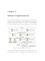
4 Software Implementation
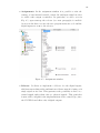
4.1 PowerTools . . . . . . . . . . . . . .
4.1.1 Setup . . . . . . . . . . . . .
4.1.2 User Program . . . . . . . . .
4.1.3 Acceleration profiles . . . . .
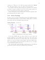
4.2 LabView . . . . . . . . . . . . . . . .
4.2.1 Software Structure . . . . . .
4.2.2 Sensors Readings . . . . . . .
4.2.3 Control Strategy . . . . . . .
4.2.4 Pressure Estimation . . . . .
4.2.5 End-runs Detection . . . . . .
4.3 Matlab . . . . . . . . . . . . . . . . .
4.3.1 Weight Distribution . . . . . .
4.3.2 Data Acquisition . . . . . . .
4.3.3 Leakage Coefficient . . . . . .
4.3.4 Pressure Estimation Function
4.3.5 Efficiency Calculation . . . . .
.
.
.
.
.
.
.
.
.
.
.
.
.
.
.
.
.
.
.
.
.
.
.
.
.
.
.
.
.
.
.
.
.
.
.
.
.
.
.
.
.
.
.
.
.
.
.
.
.
.
.
.
.
.
.
.
.
.
.
.
.
.
.
.
.
.
.
.
.
.
.
.
.
.
.
.
.
.
.
.
.
.
.
.
.
.
.
.
.
.
.
.
.
.
.
.
.
.
.
.
.
.
.
.
.
.
.
.
.
.
.
.
.
.
.
.
.
.
.
.
.
.
.
.
.
.
.
.
.
.
.
.
.
.
.
.
.
.
.
.
.
.
.
.
.
.
.
.
.
.
.
.
.
.
.
.
.
.
.
.
.
.
.
.
.
.
.
.
.
.
.
.
.
.
.
.
.
.
.
.
.
.
.
.
.
.
.
.
.
.
.
.
.
.
.
.
.
.
.
.
.
.
.
.
.
.
.
.
.
.
.
.
.
.
.
.
.
.
.
.
.
.
.
.
.
.
.
.
.
.
.
.
.
.
.
.
.
.
.
.
.
.
.
.
.
.
.
.
.
.
.
.
.
.
.
.
.
.
.
.
.
.
.
.
.
.
.
.
.
.
.
.
.
.
.
.
.
.
.
.
.
.
.
.
.
.
.
.
.
.
.
.
.
.
.
.
.
.
.
.
.
.
.
.
.
.
.
.
.
.
.
.
.
.
.
.
.
.
.
.
.
.
.
.
.
.
.
.
24
25
25
27
31
32
35
36
41
41
44
47
47
49
51
53
.
.
.
.
.
.
.
.
.
.
.
.
.
.
.
.
57
58
58
61
62
63
63
65
66
67
68
68
69
69
69
70
70
vi
5 Results and Discussion
5.1 Control Precision . . . . . .
5.1.1 Sample Cycles . . . .
5.1.2 Results and Analysis
5.2 Efficiency . . . . . . . . . .
5.2.1 Results and Analysis
.
.
.
.
.
.
.
.
.
.
.
.
.
.
.
.
.
.
.
.
.
.
.
.
.
.
.
.
.
.
.
.
.
.
.
.
.
.
.
.
.
.
.
.
.
.
.
.
.
.
.
.
.
.
.
.
.
.
.
.
.
.
.
.
.
.
.
.
.
.
.
.
.
.
.
.
.
.
.
.
.
.
.
.
.
.
.
.
.
.
.
.
.
.
.
71
72
72
73
81
81
6 Conclusions
87
6.1 Future Developments . . . . . . . . . . . . . . . . . . . . . . . 88
Appendices
90
A Electric Drive Details
91
A.1 Parameters . . . . . . . . . . . . . . . . . . . . . . . . . . . . 91
A.2 Control Connections . . . . . . . . . . . . . . . . . . . . . . . 94
A.3 Scales I/O . . . . . . . . . . . . . . . . . . . . . . . . . . . . . 95
B NI USB-6210 Specifications
98
C PowerTools listings
100
D Position Control measurement samples
101
Bibliography
106
Nomenclature
Latin Alphabet
A1
A2
Ac
Ar
Asec
B1
B2
Bc
Bd
Bl
Bv
Cec
Cep
Cf
Cic
Cip
Cs
Cs,i
d1
D1
d2
D2
Dp
dr
Eavg
area of the piston head 1
m2
area of the piston head 2
m2
piston head area
m2
area occupied by the piston rod on the piston head 2
m2
area of a boom section
m2
arm of the application point of the first segment’s mass
m
force
arm of the application point of the second segment’s
m
mass force
arm of the application point of the piston force
m
viscous damping coefficient of the pump
(N · s)/m
arm of the application point of the load’s mass force
m
viscous damping coefficient of the load
(N · s)/m
external leakage coefficient of the cylinder
m3 /s/P a
external leakage coefficient
m3 /s/P a
internal friction coefficient
−
internal or cross-port leakage coefficient of the cylinder m3 /s/P a
internal leakage coefficient
m3 /s/P a
slip coefficient
m3 /s/P a
reduced slip coefficient
−
diameter of the piston head 1
m
3
displacement of pump 1
cm /rev
diameter of the piston head 2
m
3
displacement of pump 2
cm /rev
volumetric displacement of a pump
m3 /rad
diameter of the piston rod
m
average position error during the cycle
cm
vii
viii
%
Eavg
Efin
%
Efin
Eele
Eh,1,f
Eh,1,m
Eh,1
Eh,2
Eload
Fa
Fb1
Fb2
Fc
Fc
Fc,avg
Fg
Fl
g
h
I1 , I2 , I3
Kc
Ke
Kl
Kt
l
m
mb1
mb2
mch
mh
average percent position error, compared to the
%
piston full stroke
final position error at the end of cycle
cm
final percent position error, compared to the pis%
ton full stroke
electric energy at motor terminals
J
hydraulic energy in line 1, in free-fall condition
J
and measurement condition
hydraulic energy in line 1, in measurement condiJ
tion
hydraulic energy in line 1
J
hydraulic energy in line 2
J
mechanical energy imparted to the load in order
J
to overcome the free-fall speed
arbitrary additional force on piston
N
force generated by the second segment’s mass
N
force generated by the first segment’s mass
N
force generated on the load at the piston’s rod
N
force generated or developed by the piston
N
average force acting on the piston during the moN
tion
force generated or developed by the piston
N
force generated by the load’s mass
N
gravitational constant
N (m/kg)2
height of the crane from basement to joint
m
phase currents
A
current scaling factor for the drive
A
voltage constant of the electric motor
V /rpm
load spring gradient
N/m
torque constant of the electric motor
N m/A
length of the crane’s boom
m
mass of a single weight
kg
mass of the first boom segment
kg
mass of the second boom segment
kg
mass of the supporting chain
kg
mass of the weights holder
kg
ix
ml
mt
p1
p2
pL
p1,f
p1,m
pc,avg
Ph,1
Ph,2
Phyd
Pload
pmax
Pmec
Pout
Ppot
Ppot+load
Q1,f
Q1,m
Q1
Q2
Qec
Qep
Qic
Qip
QL
QL
Qs
R1
R2
RA
RD
sp
total mass of the payload
total mass of the load referred to piston
pressure in pump forward chamber
pressure in pump return chamber
pressure difference across the pump lines
pressure in line 1, in free-fall condition
pressure in line 1, in measurement condition
average pressure in chamber 1 during the motion
hydraulic power in line 1
hydraulic power in line 2
hydraulic power delivered by the pump
work performed by the additional force only, on the load.
pressure obtained in maximum torque condition
mechanical power at the pump/motor shaft
power output of the cylinder, i.e. power acting on the
load
work performed by the gravitational force only, on the
load
work performed by the sum of gravitational force and
additional force, on the load
flow in line 1, in free-fall condition
flow in line 1, in measurement condition
forward flow to pump
return flow from pump
cylinder external leakage flow
externbal leakage flow
cylinder internal leakage flow
internal leakage flow
flow through the pump = input flow of the cylinder
load flow of a pump
slip flow (total leakage flow)
resistance of voltage divider resistor 1
resistance of voltage divider resistor 2
ratio between the piston head areas
displacement ratio between the pumps
stroke of the piston
kg
kg
pA
pA
pA
pA
pA
pA
W
W
W
pA
W
W
W
W
m3 /s
m3 /s
m3 /s
m3 /s
m3 /s
m3 /s
m3 /s
m3 /s
m3 /s
m3 /s
m3 /s
Ω
Ω
−
−
m
x
srpm
Td
tf
Tf
Tf s
tm
Tm
TNm
Tp
Tp
Ts
Vboom
Vin,d
Vout,d
Vout,speed
Vout,torque
V01
V02
V0
V1
V1 , V2 , V3
V2
VIH
VIL
VOH,e
VOH
VOL,e
VOL
Vc
Vh
Vl
Vr
x0
xc
ẋc
speed reading of the drive
damping torque of the pump
free-fall time
friction torque of the pump
full-swing of torque scale for the drive
measured time
torque at the motor shaft
torque reading of the drive
torque at the pump shaft
torque at the pump shaft
seal torque
volume of the boom
voltage input of the voltage divider
voltage output of the voltage divider
voltage output of the speed signal of the drive
voltage output of the torque signal of the drive
initial volume of cylinder’s forward chamber
initial volume of cylinder’s return chamber
dead volume of a cylinder’s chamber
volume of cylinder forward chamber
phase voltages
volume of cylinder return chamber
high voltage level of the board’s digital inputs
low voltage level of the board’s digital inputs
high voltage level of the encoder signals
high voltage level of the board’s digital outputs
low voltage level of the encoder signals
low voltage level of the board’s digital outputs
volume of a cylinder’s chamber
high threshold voltage of the relays
low threshold voltage of the relays
rated coil voltage of the relays
initial position of the piston
piston position
velocity of the cylinder’s piston
rpm
Nm
s
Nm
Nm
s
Nm
Nm
Nm
Nm
N
m3
V
V
V
V
m3
m3
m3
m3
V
m3
V
V
V
V
V
V
m3
V
V
V
m
m
m/s
xi
Greek Alphabet
α, β, γ
β
∆Eh,1
∆Epot
∆Qs
ηcyl,down
ηcyl,up
η gain
ηmot,down
ηmot,up
ηpumps,down
ηpumps,up
ηtot,down
ηtot,up
µ
ρ
ρs
θ̇p
angles of boom’s joints
◦
effective bulk modulus of the system
Pa
hydraulic energy differential in line 1
J
variation of load potential energy
J
3 2
slip flow increment rate
m /s
efficiency of the hydraulic cylinder during lowering
%
efficiency of the hydraulic cylinder during lifting
%
product of the efficiencies for the lifting and lowering
%
motion
efficiency of the electric motor
%
efficiency of the electric motor during lifting
%
efficiency of pumps and distribution line during low%
ering
efficiency of pumps and distribution line during lift%
ing
overall efficiency during lowering
%
overall efficiency during lifting
%
absolute viscosity of the fluid
Pa · s
oil density
kg/m3
mass density of common steel
kg/m3
pump shaft speed
rad/s
xii
Abbreviations
NRMM
AC
ADC
DC
DDH
e.g.
EHS
i.e.
I/O
LMS
NRMM
Pr
PWM
RMS
rpm
Non-road mobile machinery
Alternating Current
Analog to Digital Converter
Direct Current
Direct Driven Hydraulics
exempli gratia
Electric Hydraulic System
id est
input/output
Least Mean Squares
Non-Road Mobile Machinery
drive’s parameter
Pulse Width Modulation
Root Mean Square
rounds per minute
Chapter 1
Introduction and Literature
Review
Non-road mobile working machines (NRMM) are fundamental means of production in modern industry. They are employed in various fields and for
different purposes, such as mining, forest harvesting, harbour work, manufacturing and construction. This study concentrates on the investigation of
position control, efficiency and application possibilities of a novel approach
to NRMM.
The common thread, in all these dissimilar NRMM applications, is the
need of high power delivery in a contained space. For this sake, hydraulic
actuation has shown to be, and still remains, the most effective choice. One
of the strongest features of hydraulics is its straightforward capability of
working as a force transformer [1]. The hydraulic power amplification, depending on the cross-sectional areas of the piston, guarantees the possibility
to generate very high power factor in reduced spaces [2]. Moreover hydraulic
actuators work in a simple manner and can be used to transmit, produce and
store fluid power [2]. Actually, they use nearly incompressible fluid which results in a greater, more efficient and consistent work or power output [3]. This
is due to the fact that hydraulic fluid molecules are able to resist compression
under heavy load hence minimal energy loss is experienced and work applied
is directly transferred to the actuating surfaces. Moreover, hydraulic fluid
operates very well in harsh environments, demanding productive cycles and
heavy working applications [2].
Hydraulic systems have disadvantages as well. A higher constructional
weight is required in order to guarantee structural integrity in condition
1
2
of heavy loads, with addition of side components such as hydraulic lines,
reservoirs, filters, valve blocks and so on [4]. Furthermore, hydraulic fluid
is susceptible to contaminations and foreign object damage, because of its
polluting nature [5],[6]; this turns out also in a health risk for users [7],[8].
Other drawbacks are losses, such as friction and leakage [9] and the protection against rust, corrosion and dirt is required [2]. Even considering these
issues, the attempt to produce equal forces by means of magnetic fields has
been unfruitful, so far. That because, with magnetic actuation, it would be
needed 10-100 times as much axial stress in order to compete with a normal hydraulic system [1]. In practice, hydraulic systems remain the most
functional implementation, also for the future [10].
Once the oil hydraulic is chosen for working machines, the power supplying has to be considered. Machinery is often diesel operated, but trends
towards diesel-electric hybrid and fully electric operated machines are arising
[11]. Some of the issues which push technology in this direction are the constantly growing cost of mineral fuels, the air pollution derived from their employment and efficiency of diesel motors, which is usually sensibly lower than
the electric counterpart [12]. For what concerns the environmental awareness, in the latest decades regulations for harmful exhaust gases for diesel
powered equipment became more and more strict [13],[14]. In order to improve the efficiency, moreover, energy consumption and regeneration must be
considered, especially in heavy working machines [15]. For this reason hybrid
technologies are the main trend of industry and research facilities [16].
In this framework, tendency towards clean and compact electro-hydraulic
systems, which deliver powerful, linear movement with valve-controlled or
pump-controlled implementation, is observed in industry. They aim to fulfil the requirements for small size-to-power ratio, low pollution and energy
efficiency, by means of lowering losses and introducing energy recovery [17].
The most widely applied systems are valve - controlled, but they present
few relevant drawbacks, such as throttled pressure loss [18], lower efficiency
[19], cavitation [19], serious heat generation [2], non-linear modelling complexity [20] and difficult size reduction [20]. In recent investigations the pumpcontrolled electro-hydraulic servo systems directly driven by servo motor
(DDH) have appeared. These systems have the chance to overcome some of
the traditional hydraulic systems disadvantages. In the fact, pump-controlled
systems appear more compact, more reliability and highly efficient [17].
3
Various applications of DDH design strategy can be found in recent literature. In [21] the direct drive approach is implemented by means of an
electric motor controlling a variable displacement pump. The flow control
is handled by a variable displacement pump and an accumulator is used to
absorb and buffer the pressure pulses. The actuation system is employed to
control an emulsion pump and the energy regeneration capabilities in various
working conditions are analysed.
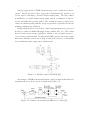
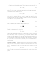
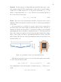
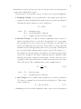
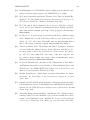
In [22] and [23], direct electric drive control implementations are proposed
in order to control a forklift with single-acting cylinder (Fig. 1.1). The results
show relevant energy saving capabilities, thanks to the potential energy recovery strategy implemented. Trend toward DDH appears also in the pump
innovation analysis carried out in [24], in which the stress is on throttling
losses elimination and compactness enhancement.
Figure 1.1: Forklift control with DDH [23]
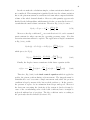
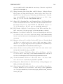
An example of DDH system in which flow control is implemented directly
regulating the servo motor speed is found in [25] (Fig. 1.2).
Figure 1.2: Rudder roll stabilization EHS servo control [25]
4
The article outlines a novel approach to rudder roll stabilization and
employs the DDH strategy - actually called Electric Hydraulic System (EHS)
in the paper - in order to reduce power consumption, size of the system and
piping complexity. It turns out in operative noise lowering as well.
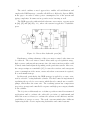
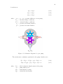
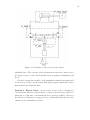
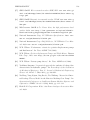
The DDH approach, with switched reluctance servo motor, appears again
in [26], [27] and [28] (Fig. 1.3), where the system is applied to a hydraulic
press.
Figure 1.3: Direct drive hydraulic press [26]
Furthermore, taking advantage of the servo motor control, other aims can
be achieved. The servo motor control allows wide speed regulation range,
high accuracy and smooth movement, since the motor motion profiles could
be finely tuned and adjusted depending on the particular system. Moreover,
the energy savings are remarkable [25], because the rotation, and consequent
power consumption of the motor, starts only when a movement is required,
in a on-demand strategy.
In this work, particularly, the DDH strategy is applied to a crane, actuated by a double - acting hydraulic cylinder. The flow control is implemented
regulating the speed of a servo motor which directly controls two reversible
pumps, which share the same axle. The resulting system has compactness
properties, prompt and controllable response and high power output, thanks
to the cylinder.
The objectives of this study are: to define a position control for automated
applications and to evaluate the achievable precision; to understand and
model the sources of losses; to evaluate the system overall efficiency and the
possibilities of energy recovery. The work concerns mainly three different
engineering fields: electric engineering, hydraulics and control systems.
5
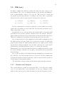
1.1
Scope of the work
The aim of this Master’s thesis is to evaluate the application possibilities of a
novel hydraulic system, analysing both automated position control precision
and system efficiency. The work focuses on employing fixed displacement
hydraulic motors, implementing the control strategy as flow control obtained
with variable speed servo motor, instead of the common and less efficient
valve control or the more complex variable displacement pump control. The
study suggests an implementation of the control strategy oriented to obtain
smooth and efficient movements, taking advantage of the servo drive capabilities. The energy evaluation is based on the analysis of the system efficiency
and on the possibility of recovering a certain amount of potential energy. The
thesis consist on modelling the system, providing and implementing a suitable control strategy, evaluating its performances and the resulting energy
balance.
1.2
Scientific contributions
This thesis contains a system engineering study of an electro-hydraulic crane,
focused on the applicable control strategy and on the efficiency of the components. The main scientific contributions follow:
• Accurate modelling of novel electro-hydraulic system, with consideration for the main sources of losses.
• Analysis and estimation of the leakage flow.
• Study of the applicability in conditions of unpredictable variable load.
• Flow control strategy implementation, based on variable speed servo
motor.
• Definition of a sensorless control strategy, basing on a pressure estimation function, obtainable from motor’s feedback.
• Efficiency evaluation of each system component and of overall system.
• Energy recovery possibilities and theoretical cycle efficiency.
6
1.2.1
List of publications
The publications concerning this work are:
1. Bonato C., Minav T.A, Sainio P., Pietola M., "Position control of direct
driven hydraulic drive”, FPNI proceedings, June 2014 (under review)
2. Minav T.A, Bonato C., Sainio P., Pietola M., "Direct driven hydraulic
drive”, IFK proceedings, March 2014
3. Minav T.A, Bonato C., Sainio P., Pietola M., "Efficiency Direct driven
hydraulic drive for Non-road mobile working machines”, ICEM proceedings, September 2014 (under review)
1.3
Outline of the work
The contents of this thesis are divided into the following 6 chapters.
Chapter 2: Description of the setup employed. The main features, ratings
and parameters of the components are outlined.
Chapter 3: Theoretical electro-hydraulic modelling of the system. The
control equations are derived, the leakage modelling and the pressure estimation curve are described. The load is modelled from a physical point of
view. At last, the efficiency equations are calculated and explained.
Chapter 4: Description of the control strategy implementation. Control
logic and employed software (PowerTools, LabView) are explained. A brief
report of Matlab calculations for efficiency is given.
Chapter 5: Main results concerning both control performance and efficiency. The numerical outcomes of measurements are listed and analysed.
Chapter 6: Conclusions from the work. The main findings are summed
up. Potential applications and advise for future development are discussed.
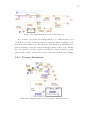
Chapter 2
Description of the System
In the following chapter an accurate description of the test setup is given. The
reader is made aware of the system structure and of its main characteristics.
The final aim is to be able to understand all the following procedures in
which the hardware is involved and, also, to make the system completely
reproducible. When the thesis project started, the main structure of the
setup was already built in the automotive laboratory of Aalto University.
Therefore, the sections of this chapter concerning this topic will be merely
descriptive. The whole control interface, the wirings of sensors, input/output
signals and acquisition systems, instead, were implemented as part of this
thesis work. For this reason the sections concerning control part will be
more exhaustive.
For further information, references to user manuals and datasheets will
be given for each component.
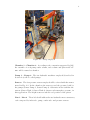
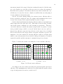
A picture of the mechanical system employed for this research is shown
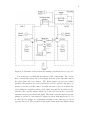
in Fig. 2.1, while its schematic description can be found in Fig. 2.2.
2.1
Setup Overview
First of all, some naming conventions for the various components of the
system will be stated. They will make the descriptions quicker and help an
easier understanding of the topic. These names will be kept for the whole
document. The reader is advised to compare the given names with the system
parts reported in Fig. 2.2.
7
8
Figure 2.1: Setup employed
Chamber 1 - Chamber 2 According to the convention suggested by [29],
the ensemble of each pump outlet volume, tube volume and piston side volume will be named as chamber.
Pump 1 - Pump 2 The two hydraulic machines employed (described in
Section 2.4) will be called pumps.
Sensors The four pressure sensors employed will be referred with the names
stated in Fig. 2.2. In the chambers the sensors reveal the pressure built by
the pumps (Sensor Pump 1, Sensor Pump 2). Otherwise in the tank line the
sensors (Sensor Tank 1, Sensor Tank 2) always read atmosphere pressure, in
this application. The height sensors reads the real position of the piston.
Line 1 - Line 2 These labels will address the two hydraulic macro-structures,
each composed by inlet tube, pump, outlet tube and pressure sensors.
9
Figure 2.2: Schematic of the system (for naming conventions refer to page 2.1)
Let us now proceed with the description of the components. The electric
drive converts three-phase AC power supply from the power line and controls
the three-phase AC servo motor. The shaft angular speed is its control
quantity, that means it is forced to follow the reference given by the drive, by
means of closed-loop PID control. Actually the motor gives as feedback the
real readings for angular position of the shaft, through the in-built encoder,
and the active current output, which can be directly converted to obtain the
amount of torque generated at the shaft. The shaft rotation is delivered to the
pumps by means of a mechanical T-shaped gearbox with fixed ratio (1,5:1)
so that the two pumps are constantly rotating at the same speed, but in
opposite direction. The provided torque splits between the two shafts basing
10
on the amount of resistance to the movement required by each hydraulic line.
Each pump, while rotating delivers to the hydraulic line a certain amount
of oil flow, from tank to cylinder or in the other way round. For example,
during lifting movement, pump 1 rotates clockwise and the oil flows from
the tank through the tube up to the cylinder, while the pump 2 works in
opposite direction, generating oil flow from cylinder to tank.
During the lifting movement, the force generated by the pressure built
in chamber 1, acting on the first piston head, must be higher than the one
induced by the payload, in order to let the piston move. During the lowering
movement, instead, the pressure in chamber 1 slows down the free-fall of the
load, obtaining a controlled lowering motion. During both the movements,
pump 2 is supposed to work together with the first one, accompanying it.
The final aim of pump 2 would be to give to the system the possibility
to deliver power in the way down as well. In fact, the setup is implemented
as a test bench for different future applications. For example, in a non-road
mobile working machine (NRMM), such as a mine loader, during a working
cycle could be required not only the ability of lifting and lowering weights, but
also the capability to generate force from up to down, typically for digging
the soil. In that scope, the stiff reference chamber would be the second one
and pump 1 would operate accompanying the movement.
Concerning the sensors, the system has been equipped with four pressure
sensors to keep the pressure checked both in the chambers and in the discharging pipe to the tank. For the application studied in this thesis work,
only the 2 transducers in the pumps side will be used, while the other 2
remain available for future application. For example, a hydraulic closed-loop
setup in which the whole system is supposed to work under pressure. The
tank line would be kept under pressure as well, actually replacing the tank
with a hydraulic accumulator.
Moreover, a height sensor for the cylinder’s piston movement was installed. The sensor, a wire incremental encoder, gives continually the actual
position of the piston during every movement. The sensors were used for
programming and testing purpose only. Actually, the final aim is not to
use them for the control strategy, taking advantage only of the information
coming from the motor feedback.
As an interface between the hardware system and the control software,
a USB acquisition board was employed (see Section 2.8). The board has
11
the capability to read some analog and digital inputs and to write on digital
outputs. Its purpose is both to convoy the information obtained from the
pressure transducers, from the wire encoder, from the outputs of the drive
and to write on the digital inputs of the drive to actuate particular control
strategies which will be explained in Section 4.2. It’s interesting to notice that
2 particular conditioning system had to be done: a voltage divider to make
the encoder output readable by the board and a relays system to amplify
the digital outputs of the board, to make them sensible for the drive. These
devices will be properly described in Section 2.8.
As can be seen in the schematic (Fig. 2.2), the payload is modelled by
second order system with the presence of mass, damper and spring.
2.2
Electric Drive
The electric drive employed for the test setup is Emerson Control Techniques
Unidrive SP1406. Its complete description can be found in the manuals [30],
[31] and a picture is shown in Fig. 2.3.
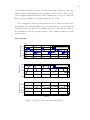
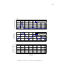
In this section, the main characteristics of the drive will be listed, starting
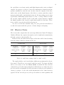
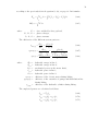
from the ratings, which are shown in Tab. 2.1.
Normal Duty
Heavy Duty
Maximus
continuous
output current,
[A]
Nominal
power
at 400V,
[kW ]
Motor
power
at 460V,
[kW ]
Maximus
continuous
output current,
[A]
Nominal
power
at 400V,
[kW ]
Motor
power
at 460V,
[kW ]
11
5,5
5,5
9,5
4,0
5,5
Table 2.1: 400V drive ratings (380V to 480V ± 10%)
The employed drive can be used in three different operating modes: OpenLoop mode, Closed Loop vector mode and Servo mode. To pursue the final
aim, it is necessary to use the Servo mode, in which the drive directly
controls the speed of the motor using the feedback device to ensure the rotor
speed is exactly as demanded. In effect the motor feedback, speed and direct
current, is going to be the only useful information in the control strategy
applied. For the research process, the speed is taken as control quantity and
12
Figure 2.3: Emerson Control Techniques Unidrive SP1406
the torque (obtained from the direct current) is used to obtain additional
knowledge about the system status.
2.2.1
Parameters and Control Connections
The tuning of the drive’s behaviour is obtained by setting the drive’s parameters. Although some of the parameters are fundamental for the thesis
process, in fact, an accurate description of them could result cumbersome in
this early part of the work. Mainly for this reason it was decided to dedicate the Appendix A.1 to this aim, the reader is advised either to go quickly
through it, or to consult it on need.
Another fundamental feature of the drive is the presence of connections
which make it accessible and allow to get information from it. The previous
reasoning over the parameters remains valid, thus the reader is addressed to
Appendix (A.2) for a brief explanation of the useful connections.
13
2.2.2
Scales I/O
The input/output terminals get and give information from and to the outside
world, in particular these terminals are supposed to communicate with the
NI USB Board (Section 2.8). For practical purposes it is necessary to keep
in consideration type, scale and amplitude of these signals. On the one hand
to avoid physical problems (such as: signals too weak to be read, signals
too strong can damage the system), on the other hand to be able to convert
properly voltage or current outputs to significant physical quantities.
From the physical point of view, the voltage operating mode is chosen
for this setup because the wirings are sufficiently short not to generate a
sensible voltage drop which could influence the accuracy of the readings.
The analog ports of the drive are designed to give as output voltage values
in the range [−10 : 10] V, which means perfect match with the ratings of
the NI USB board. Otherwise the digital input ports of the drive work in
the range [0 : 24] V (where 0 V is the logic 0 and 24 V is the logic 1), while
the NI board writes digital outputs in the range [0 : 5] V. To overcome this
difference a relay for each digital line has to be used, their implementation
is explained in the next paragraph (Par. 2.2.3).
As it comes to the conversions, it is necessary to understand properly
the scales of the analog outputs to obtain precise readings of the quantities. The procedure finalized to obtain the right conversions, the parameters
involved and the interesting results, which will be referred in the software
implementation (Chap. 4), are described in Appendix A.3.
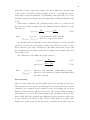
2.2.3
Relays
As previously remarked in this section, the presence of relays employed as
an interface between the output of the NI USB board and the Drive digital
input terminals appears to be necessary. To this aim Omron G6J-2FL-Y
signal relays have been chosen, for an exhaustive description, ratings and
characteristics the reader is addressed to the manufacturer’s datasheet [32].
The main features of these relays are the coil voltage (rated Vr = 5V with
threshold Vl = 0, 1 · Vr and Vh = 0, 75 · Vr ) and the contact rated voltage (up
to 30 A), which make these devices the optimal choice for the system. In
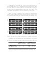
Fig. 2.4, an excerpt from the datasheet is shown.
14
Figure 2.4: Employed relay type (Omron [32])
2.2.4
Drive Software
A basic control software is provided by Emerson: PowerTools. This tool is
needed to communicate with the drive, download user programs in it, access
and modify the system variables, shape the control signals for the movement,
assign input and outputs to internal variables, implement a Selector for the
digital inputs, define simple control strategies and set home position. This
software is not powerful enough (for example it can’t integrate the speed) to
manage the position control of an hydraulic system. Therefore, it is used for
configuration of the device and for low level commands (such as move up,
move down, stop, move home). The high level part of the control strategy is
handled by LabView (Section 4.2).
The main characteristic of the PowerTools configuration employed and
their settings will be outlined in Section 4.1, along with the explanation of
user program for the control logic.
2.3
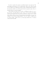
Electric Motor
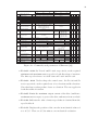
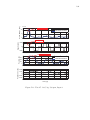
The chosen motor for this setup is Emerson Control Techniques Unimotor
FM115 U2C300 VACAA115190, its exhaustive description can be found in
the datasheet [33] and a picture is shown in Fig. 2.5.
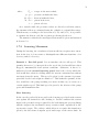
Stall
torque,
[N m]
Peak
torque,
[N m]
Rated
torque,
[N ]
Rated
speed,
[rpm]
Max
speed,
[rpm]
Stall
current,
[A]
Rated
power,
[kW ]
Drive
VPWM,
[V AC]
9,4
37,6
8,1
3000
4800
5,9
2,54
380/480
Table 2.2: Motor ratings
15
Unimotor FM is a high performance brushless permanent magnet AC
servo motor, matched to use for Control Techniques drives. The ratings for
this particular model are shown in Tab. 2.2.
Other relevant parameters of the employed motor are:
Kt = 1, 6 Nm/A
(2.1)
Ke = 9, 8 · 10−2 V/rpm
(2.2)
where: Kt is the torque constant of the motor (i.e., torque in Nm per Ampere
of torque producing current); Ke is the voltage constant, i.e., ratio between
RMS line to line voltage produced by the motor and the speed, in V/rpm.
Figure 2.5: Emerson Control Techniques Umimotor FM115
As can be seen in Fig. 2.5, on the motor side opposite to the mechanical
shaft, there are two electric connectors: one is the power plug which carries
the AC three-phase PWM supply from the drive; the other one is the signal
plug, which carries low-voltage power supply for the encoder and gets its
feedback.
In this particular model of servo motor, the feedback device fitted is
an incremental encoder with 4096 pulses per revolution and 5 V dc supply
voltage. This device uses an optical disc. The position is determined by
counting steps or pulses, 2 sequences of pulses in quadrature are used so
the direction sensing may be determined. A marker pulse occurs once per
revolution and is used to zero the position count. The encoder also provides
commutation signals, which are required to determine the absolute position
during the motor phasing test. Positional information is non absolute - i.e.
position is lost when the drive is powered down.
16
2.4
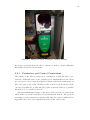
Hydraulic Motors
The employed hydraulic reversible motors are Vivoil XV-2M/14 and XV2M/22 with external drainage, a picture is given in Fig. 2.6. For their complete description the reader is addressed to the manufacturer’s datasheet [34].
Figure 2.6: Vivoil XV series
A reversible motor is a device which can operate both as a motor (generating mechanical energy as shaft rotation from oil flow) and as pump (delivering
hydraulic flow from shaft rotation). It can also rotate in both the counterclockwise and clockwise directions. In this application the motors are used as
pumps during the lifting movement and as controlled motors during the lowering one. Moreover, these hydraulic machines need to be capable of rotating
in both the directions since the T-shaped gearbox imposes opposite rotation
to them. In effect while one delivers oil to the chamber, the other one must
suck oil from the other side, in order to produce a harmonic movement of
the actuator.
From this former description, it is easy to understand how in this particular application the role of the reversible motors employed is a mixture of
motoring and pumping in each cycle. For this reason, in the following, these
hydraulic devices will be referred as pumps (according to the conventions
stated in the beginning of Section 2.1). In the case the motor classification
will be needed, the reason will be carefully explained for each particular case.
Two different pumps are used for the setup, these devices behave in identical way and have the same characteristics, the only difference between them
17
is the displacement. For line 1 the bigger one is installed (22,8 cm3 /rev),
while for line 2 the smaller one (14,4 cm3 /rev). This inequality between the
two lines is due to the different head areas of the piston. Actually, as it
will be explained extensively in the next section (Section 2.5), the employed
cylinder presents asymmetry between head areas. This asymmetrical configuration must be preserved in the sizing of the pumps as well (this assumption
will be explained and demonstrated in Chap. 3).
Anyway, it is worth deducing the ratio between displacements, since it is
going to be a fundamental value in the forthcoming discussions:
RD =
D2
' 0, 63 = 63%
D1
(2.3)
where RD is the ratio between pump displacements, D1 is the displacement
of pump 1, D2 is the displacement of pump 2.
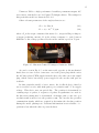
Figure 2.7: Example of an external gear pump
As a last remark, relevant construction characteristics of these hydraulic
machines and their installation will be outlined. They are external gear
pumps, which means the oil is convoyed from the inlet to the outlet by means
of two meshed gears (Fig. 2.7). The flow could go from tank line to piston
chamber or the other way round, depending on the particular movement.
Even though close tolerances are held between the housing and the gear side,
some clearance is needed to allow the movement. Therefore, as any other
hydraulic machine, they are bound to have a certain amount of leakage,
which is convoyed towards the drainage and discharged back into the tank.
18
2.5
Cylinder
The setup is equipped with a Pikapaja MIRO C-10-60/30x400 A-55 hydraulic
cylinder used as actuator for the crane, its extensive description can be found
in the datasheet (in Finnish) [35] and a picture is shown in Fig. 2.8.
Figure 2.8: Hydraulic Cylinder MIRO C-10-60
The device is a common double-acting cylinder, which means it has two
chambers separated by the piston head. Each chamber is fed by its own
orifice and the sealing of the piston head is supposed to be highly reliable in
order to neglect the leakage between chambers.
It is worth noticing, as previously outlined, that the head areas are different in the two sides of the piston. From the datasheet:
d1 = 0, 060 m ,
(2.4)
dr = 0, 030 m ,
(2.5)
sp = 0, 400 m ,
(2.6)
where d1 is the piston head diameter (side 1), dr is the rod diameter and sp
is the stroke.
19
From values (2.4) and (2.5), it is easy to derive the areas. The second
head surface is obtained as a difference between the whole area and the one
occupied by the rod:
A1 = π ·
Ar = π ·
d1
2
2
dr
2
2
= 2, 8274 · 10−3 m2
(2.7)
= 7, 0686 · 10−4 m2
(2.8)
A2 = A1 − Ar = 2, 1205 · 10−3 m2
(2.9)
where A1 is piston head area side 1, Ar is piston rod area, A1 is piston head
area side 2.
Finally, the ratio between head areas RA is calculated as:
RA =
2.6
A2
' 0, 75 = 75%
A1
(2.10)
Sensors
In this section all the sensors employed in the system are described and their
function is outlined.
2.6.1
Pressure Transducers
The chosen pressure transducers are Gems 3100R 0400S (Fig. 2.9), for further
details refer to the datasheet [36].
Figure 2.9: Pressure Transducer Gems 3100R
This kind of sensor takes advantage of a thin film of semiconductor, deposed by sputtering, which, when a certain pressure is applied, modifies its
geometry (strain). The strain in semiconductor thin films causes variation
20
of electrical resistivity, this phenomenon is detected as piezoresistive effect.
All in all, the transducer works as strain gauge, measuring the resistivity
opposed to the supply current, it gives a precise and repeatable measure of
the applied pressure.
Those particular sensors are designed to bear pressures in the range
[0 : 400] bar, giving as an output a voltage value in the range [0 : 5] Volts,
which varies with the gradient of resistance. The output suits perfectly the
range of NI USB board analog inputs (which can be set to ±5 V, while
the maximum amplitude is ±10 V) and does not need to be attenuated nor
amplified. The pressure scale of the sensors is slightly oversized, in this application, peaks of pressure not higher than 105 bar are observed indeed, but
still sufficiently precise for the purpose.
It is worth remarking, these sensors were employed in order to evaluate
the system efficiency, to collect data for improving the quality of control logic
and to keep system behaviour under observation. But then, the final goal
is to define a control which does not take advantage of the pressure values
information, which means they would not be needed in a real application.
2.6.2
Height sensor
A SIKO SGI3500 wire-actuated encoder is installed to serve as a sensor
for the piston displacement. This sensor is composed by the wire SGI
drum (datasheet [37]), coupled with the SIKO IV58M incremental encoder
(datasheet [38]). A picture of the complete sensor is given in Fig. 2.10a.
(a) Height sensor
(b) Digital output signals
Figure 2.10: Wire-actuated encoder SIKO SGI3500
The main housing of the sensor is fastened against the cylinder barrel,
while the terminal of its wire is fixed to the piston rod-end head. A stainless
steel cable is wound up around the drum inside the housing. When the piston
21
moves, the cable unwinds following the movement, that causes the rotation
of the drum. The drum is tied to the encoder flange, an optical disc, whose
holes generates 3 different digital signals: A, B and 0 (Fig. 2.10b). This
particular encoder has a resolution of 2560 pulses/revolution, that means
signals A and B rise 2560 times per revolution, while 0 rises one time per
revolution, it is called marker since it is used as a reference to define the zero
position.
A and B are called quadrature outputs, as they are 90 degrees out of
phase. This feature is fundamental to understand the direction of the movement: either A rises first, so the drum is spinning clockwise and the piston is
moving forth; or B rises first, so the drum is spinning counter-clockwise and
the piston is moving back.
To translate the train of pulses into an angular position measure a counter
is needed, in this application NI USB-6210 board internal counter is used
(Section 2.8). Finally, considering the drum circumference it is easy to transfer the angular measure in a linear one. For this particular encoder the linear
resolution is 10 pulses/mm.
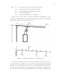
It is worth noticing that the output digital signals of the encoder have
threshold levels VOL,e = O, 5 V and VOH,e = 29, 2 V, that means these signals must be attenuated in order to make them compatible with the board
specifications (VIL = O V and VIH = 5 V (see Section 2.8). Therefore, it is
necessary to implement a voltage divider (Fig. 2.11a) with the same characteristics for each of the three channels. The task is accomplished by means
of three couples of resistors, with R2 = 120 kΩ and R1 = 24 kΩ. In effect,
following the theoretical scheme in Fig. 2.11b, the resulting voltage for the
high level is:
R1
· Vin,d ' 4, 87 V
(2.11)
Vout,d =
R1 + R2
Likewise for the pressure sensors, the height sensor has its role during
control logic set up, efficiency measurements and observation of system behaviour. On the contrary, in the final stages the control technique is supposed
to set the position neglecting encoder’s information.
22
(a) Implementation
(b) Scheme
Figure 2.11: Voltage divider
2.7
Mechanical T-shaped gearbox
For the aim of delivering the motion generated by the electric motor to
the hydraulic pumps shafts, a MS-Graessner P-90-FL fixed-teeth T-shaped
gearbox was employed (Fig. 2.12). An exhaustive description can be found
in the datasheet [39].
Figure 2.12: Mechanical T-shaped gear
Its behaviour is straightforward: the gear delivers the motion reducing
the module of the speed of one third (transmission ratio 1,5:1) and inverting
the direction on each pump shaft.
Regarding the power efficiency, the declared efficiency of the gearbox is
98%. This value is confirmed by an accepted rule of thumbs in engineering: it
23
is assumed a loss of 1% efficiency each 90◦ turn in a mechanical shaft. Hence,
across this work, it will be hypothesized that the sum of the mechanical
energy transferred to the two pump shaft be roughly around 98% of the
power measured at the electric motor shaft.
2.8
NI USB Board
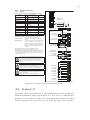
The employed board is Nation Instruments NI USB-6210, its detailed specifications can be found in the datasheet [40] and for further explanation about
the board capabilities and behaviour refer to the user manual [41]. A picture
is given in Fig. 2.13.
Figure 2.13: NI USB-6220 board
The main purpose of the board is to link the real system with the control
part. It actually convoys each output from the setup sensors and from the
drive, samples them and get readings of their values. Furthermore, by means
of its digital outputs delivers control signals to drive inputs, allowing the
control strategy implementation.
The main specifications and a wiring scheme can be found in App. B.
2.9
Crane
The main structure of the setup is a Masters Craneworks Vestas FC 1100
small crane (see Fig. 2.1 at page 8). The height from base to joint is 1, 55 m,
while the boom length is l = 1, 67 m. An accurate analysis and modelling
will be given in Section 3.1.
Chapter 3
Theoretical Model
In the present chapter, the employed system model is precisely described
and analysed. The theory followed in order to model the hydro-mechanical
part is mainly taken from Merritt’s work [29]. Other contributions, regarding
leakage modelling and efficiency, are obtained from Wilsons’ work: [42],[43]
and [44].
The employed system can be modelled as a pump-controlled hydraulic
double-acting linear actuator. Pumps and motors are used to convert mechanical energy into hydraulic energy and vice versa, respectively. These
machines may be divided in hydrodynamic or positive displacement. Hydrodynamic machines are not suited for control purposes.
According to [29], in positive displacement machines, fluid passes through
the inlet into a chamber which expands the volume and fills it with fluid.
The volume expansion causes a shaft rotation in a motor, in contrast to a
pump where volume expansion is caused by shaft rotation. The volume of
trapped fluid is sealed from the inlet by some mechanical means and then
transported to the outlet side where it is discharged. A succession of small
volumes of fluid transported in this manner gives a fairly uniform flow. Thus
a positive or definite amount of fluid is displaced through the machine per
unit of shaft revolution. Positive displacement machines are quite efficient
and find extensive use in control systems.
The pumps employed for the test setup are positive fixed-displacement
machines, therefore, they will be modelled according to this description.
Moreover, these machines are continuous travel devices (in detail external
gear pumps), which means they have a lever mechanism (gear radius) to
which the shaft torque is applied; a mechanical element (gear’s meshed part)
24
25
to convert this force from shaft torque into flow and build pressure; some
method to seal inlet from outlet (gear coupling); some method of porting
fluid to the mechanical elements on which the pressure acts (hoses).
The cylinder used for the test setup, in contrast, is a limited travel device,
since it is linear and there is not any flow between inlet and outlet (besides
the leakage one). In this kind of devices the inlet flow is used to build pressure
which acts on the piston head in order to contrast the force generated by the
load and produce movement. The modelling and basic description of these
machines is usually more straightforward and they are characterized by a
high efficiency.
3.1
Electro-hydraulic and Mechanical Model
In order to obtain a global model for the system, it is necessary to start
modelling each component, first with its ideal description and then adding
the corrections to consider non-idealities. At a later stage these models will be
linked by a relation considering the system construction and taking advantage
of the continuity equations for hydraulics.
For this particular setup, the whole system will be modelled as a pump
controlled cylinder, in which the pumps have constant displacement but the
flow control is achieved varying the input speed at the shaft. This kind of
system, compared to the valve controlled type, has the advantage of a high
theoretical efficiency, but it is often characterized by a slower response (motor
start-up); requirement of a servo motor to control the flow; necessity of close
coupling of pumps and actuator [29]. These requirements and characteristics
will be kept in consideration during the modelling stage and their influence
on the system will be described.
3.1.1
Ideal Pump and Cylinder Analysis
An ideal pump or motor is defined as having no power losses due to friction
and leakages and, consequently, has an efficiency of 100%. Although this
is certainly not true in practice, hydraulic machines are quite efficient, and
system design is often based on ideal machines [29] and non-idealities are
added in a later phase, upon need.
26
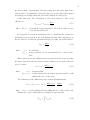
Consider an ideal hydraulic pump. The mechanical power input Pmec is:
Pmec = Tp θ̇p
(3.1)
where: Tp is the torque at the pump shaft and θ̇p is the pump shaft speed.
The hydraulic power output (Phyd ) is:
Phyd = pL QL
(3.2)
where pL is the pressure difference across the pump lines and QL is flow
through the pump. Because the pump is assumed to be ideal, the equations
(3.1) and (3.2) can be equated to yield:
Tp =
QL
pL
θ̇p
(3.3)
Now, by definition, the volumetric displacement (Dp ) is:
Dp =
QL
θ̇p
(3.4)
Finally, by substitution of (3.4) in (3.3):
Tp = Dp pL
(3.5)
which is the fundamental relation for an ideal pump (or motor, swapping
input and output). Only one parameter (Dp ) is required to define the ideal
machine, and this quantity is also the single most important parameter for
practical machines. This analysis also holds for the ideal motor, except that
the power flow is reversed, that is, hydraulic power is transformed in mechanical power.
Hydraulic Cylinder A similar analysis can be made for an ideal cylinder.
The piston area is the parameter analogous to the displacement of a rotary
device. In particular, in order to calculate the power acting on the load
(Pout ):
Pout = Fc ẋc
(3.6)
where Fc is the force generated at the piston rod and ẋc is the velocity of the
piston.
27
Since the cylinder is assumed to be ideal, power input (3.2) can be equated
to power output (3.6) to yield:
Fc =
QL
pL
ẋc
(3.7)
Now, the volume of the cylinder’s chamber (Vc ) is:
Vc = V0 + Ac xc
(3.8)
where: V0 is the dead volume of the cylinder’s chamber, Ac is the piston head
area and xc is the piston position.
Its variation corresponds to the input flow (QL ):
QL =
Vc
= Ac ẋc
dt
(3.9)
Then, by substitution of (3.9) in (3.7):
F c = A c pL
(3.10)
which is the fundamental relation for an ideal cylinder. As previously stated,
the parameter Ac plays the same role as Dp for the ideal pump. Only difference is that the piston, by its nature of linear actuator, is defined also by the
length of the maximum movement (stroke of the piston), while this is absent
in a rotary machine.
3.1.2
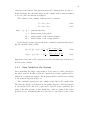
Practical Pump and Cylinder Analysis
Leakage flow and friction are the sources of losses in hydraulic machines.
In this section these losses will be examined and included in the analysis
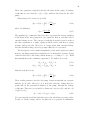
of steady state performance. Consider the schematic of the gear pump in
Fig. 3.1. It is apparent that two type of losses can exist: internal or cross-port
leakage between the lines and external leakage from each pump chamber, past
the gears, to the case drain. Because all mating clearances are intentionally
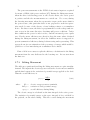
made small to reduce the losses, these leakage flows are laminar [43].
The internal leakage (Qip ) is proportional to motor pressure difference,
while the external leakage (Qep ) in each chamber is proportional to the particular chamber pressure (assuming negligible drain pressure), and they can
28
be written as:
where
pL
Cip
Cep
p1
p2
=
=
=
=
=
Qip = Cip pL
(3.11)
Qep1 = Cep p1
(3.12)
Qep2 = Cep p2
(3.13)
p1 − p2 = pressure difference across pump,
internal leakage coefficient,
external leakage coefficient,
pressure in forward chamber,
pressure in return chamber.
Figure 3.1: Schematic diagram of a gear pump
The steady-state continuity equations for the pump chambers are:
where
Dp
θ̇p
Q1
Q2
=
=
=
=
Q1 − Cep p1 − Cip (p1 − p2 ) − Dp θ̇p = 0
(3.14)
Dp θ̇p + Cip (p1 − p2 ) − Cep p2 − Q2 = 0
(3.15)
ideal volumetric displacement of the pump,
pump shaft speed,
forward flow to pump,
return flow from pump
29
These two equations completely describe the flows in the pump. If leakage
coefficients are zero then Q1 = Q2 = Dp θ̇p , which is the result for the ideal
pump.
Subtracting (3.15) from (3.14) yields
Cep
pL
QL = Dp θ̇p + Cip +
2
(3.16)
where by definition
Q1 + Q2
(3.17)
2
The quantity QL , commonly called load flow, represents the average quantity
of the flows in the two pump lines; QL equals the flow in each line only if
external leakage is zero. The concept of load flow is useful because it reduces
two flow equations to a single equation which relates load flow to pump
pressure and speed only. Moreover, it clearly shows that external leakage
acts like internal leakage as far as pressure difference is concerned.
The description can be further simplified because in the employed control
strategy, the input pump line is assumed to be at atmosphere pressure (being
connected directly to the tank), which means p1 = 0 and pL = −p2 . With
this simplification the continuity equations (3.15) and(3.14) become:
QL =
Q1 + Cip p2 − Dp θ̇p = 0
(3.18)
Dp θ̇p − (Cip + Cep )p2 − Q2 = 0
(3.19)
And the load flow (3.16):
Cep
QL = Dp θ̇p + Cip −
p2
2
(3.20)
These results permit to describe the pump behaviour through one pressure
and the speed only. Moreover, it is noticeable that the leakage flow depends only on the pressurised chamber of the pump, through the leakage
coefficients. Therefore it is possible to define the slip flow (Qs ) and the slip
coefficient (Cs ):
Qs = (Cip + Cep ) p2 = Cs p2
(3.21)
Qs represents the total flow which decreases the ideal flow at pump outlet,
because of all the leakage effects. In this way it is possible to summarize
30
the effect of the leakage with one parameter. A deeper description of this
parameter and its derivation will be given in Section 3.2.
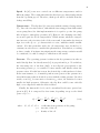
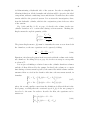
Hydraulic Cylinder As far as the hydraulic cylinder is concerned, a practical analysis of it must include the effects of the leakage flow. For this type
of power element, the leakage is due to the seals. There are external leakage
(Qec ), around the rod, and internal leakage (Qic ), around the piston head,
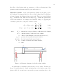
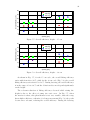
between the chambers. According to the schematic in Fig. 3.2, applying the
continuity equation to each piston chamber yields:
dV1 V1 dp1
+
dt
β dt
dV2 V2 dp2
Cic (p1 − p2 ) − Cec p2 − Q2 =
+
dt
β dt
Q1 − Cic (p1 − p2 ) =
where
Cic =
Cec =
β=
p1 , p 2 =
Q1 , Q2 =
V1 , V 2 =
t=
(3.22)
(3.23)
internal or cross-port leakage coefficient of the cylinder,
external leakage coefficient of the cylinder,
effective bulk modulus of the system (Section 3.5),
pressure in forward and return chamber,
flow in forward and return chamber,
volume of forward and return chamber,
time.
Figure 3.2: Schematic diagram of a double-acting cylinder
At right hand of continuity equation, there are two terms. The first one
keeps in consideration the volume variations due to the displacement of the
piston, while the second term concerns the pressure variations due to the
31
elasticity of the system. This phenomenon will be illustrated in Section 3.5.
In the following, the external leakage for the cylinder will be always assumed
to be zero, since its amount is negligible.
The volumes of the cylinder chambers may be written:
where
A1 , A2
xc
V01
V02
=
=
=
=
V1 = V01 + A1 xc
(3.24)
V2 = V02 − A2 xc
(3.25)
piston heads areas,
displacement of the piston,
initial volume of the forward chamber,
initial volume of the return chamber.
Replacing the volume expressions in the continuity equations and neglecting the external leakage yields:
V01 + A1 xc dp1
xc
Q1 − Cic (p1 − p2 ) = A1 +
dt
β
dt
xc
V02 − A2 xc dp2
Cic (p1 − p2 ) − Q2 = −A2 +
dt
β
dt
(3.26)
(3.27)
Equations (3.26) and (3.27) completely describes the hydraulic behaviour of
double-acting cylinder.
3.1.3
Joint Model for the System
After modelling the single components it is necessary to built a model for
the whole system. In this section the equations previously outlined will be
unified in a common description. The derivation will be carried out according
to the symbols depicted in Fig. 3.3.
The continuity equations for the cylinder (3.26) and (3.27) remain valid.
The flows Q1 and Q2 are delivered by the pumps, therefore, their description
is obtained in (3.14) and (3.15), and can be replaced in the equations. For
pump 1 the inlet pressure is zero (tank line), while for pump 2 the outlet
pressure is zero. Remarking that θ̇p is forced to be the same because of the
32
Figure 3.3: Schematic diagram of the whole system
gear box, yields:
xc
V01 + A1 xc dp1
Dp1 θ̇p − Cs1 p1 − Cic (p1 − p2 ) = A1 +
dt
β
dt
V02 − A2 xc dp2
xc
Cic (p1 − p2 ) − Cs2 p2 − Dp2 θ̇p = −A2 +
dt
β
dt
(3.28)
(3.29)
Equations (3.28) and (3.29) model the hydraulic behaviour of the global
system. It is now necessary to build a proper model of the leakage flow, in
order to completely define the left hand terms of the equation, and of the
load, so that the relation between pressure and force acting on the piston
rod can be found. In the following Section the model of the leakage will be
derived, while in Section 3.3 the payload will be discussed.
3.2
Leakage Model
In this section, the leakage flow is analysed for one of the hydraulic lines
of the system. In particular, from (3.28), it is apparent that two terms are
mostly relevant for the description of leakage flow: slip flow of the pump and
33
cross-chamber flow of the cylinder.
As a first simplification, the internal leakage flow of the cylinder will
be neglected. This assumption is acceptable because, as stated in [2], the
overall efficiency of this linear actuator is mainly influenced by frictional
losses encountered by the piston and rod during its stroke. As a matter of
fact, the common approach to overall efficiency for linear actuators does not
even keep in consideration the leakage, but only the torque efficiency.
Moreover, the leakage coefficient of the pump will be evaluated empirically, which implies the effect of the cylinder leakage will be fairly included
in the total leakage. For these reasons, the continuity equation for side 1
(3.28) can be written as:
xc
Dp1 θ̇p − Cs1 p1 = A1 +
dt
V01 + A1 xc
β
dp1
dt
(3.30)
Let us proceed in the analysis of the pump leakage; for this purpose [29]
gives a first very basic model of it. The slip flow is usually laminar and,
therefore, inversely proportional to the viscosity [29]. Test results also indicate that the slip flow is related to motor displacement. Hence:
Qs = Cs p = Cs,i
where
Dm
p
µ
(3.31)
Cs,i = reduced slip coefficient,
µ = absolute viscosity of the fluid.
Once the constant contributions to the slip coefficient are separated, it
is necessary to understand which are the variables influencing the leakage in
a gear pump. Interesting and detailed analysis of the topic is carried out in
[45]. Where the author analyses the effects of operating conditions, such as
pressures, speeds and oil temperatures, on the leakage flow characteristic for
various type of gear pumps. An even more detailed internal leakage model,
specialized for exterior meshing gear pumps, can be found in [46]. In this
work the different causes of flow losses are divided and particularized for the
sake of obtaining a mathematical model of the global flow. The results of the
previously introduced articles ([45] and [46]) are at the basis of the following
leakage flow modelling.
34
Speed In [45], tests were carried out at different temperatures and for
different pumps. The results show that the flow losses are almost independent
from the operating speed. Therefore, shaft speed will be excluded from the
leakage modelling.
Temperature The slip flow (Qs ) increases with the raising oil temperature
(To ), since the viscosity reduces, and with the increasing pressure differential
across pump lines (for this implementation it is equal to p1 sine the pump
inlet is kept to atmosphere pressure) [45]. However, the changing rates ∆Qs
are nearly equal for all oil temperatures. Which means, when the temperature increases, the viscosity of the oil decreases and, being under the fraction
sign, forces the Qs vs. p1 characteristic to raise, without sensible modifications. For this particular work, the oil temperature was checked to be
constant, in order not to consider this phenomenon. Nonetheless, according
to these results, if in future investigations the temperature variation would
be considered, it could be simple to add them to the model.
Pressure The operating pressure is taken as the key parameter in order to
model the slip flow. As already stated, Qs is proportional to p1 . Nevertheless,
the increasing rate of the flow (∆Qs ) is not directly proportional to the
increasing pressure p1 , it actually becomes smaller and smaller when the
pressure raises. For this last reason, the desired slip coefficient has to behave
in the same manner; i.e., it must depend on some powers of the pressure in a
way which assures that it slowly decreases with the raising pressure. In other
words, even if Qs becomes more relevant as p1 raises, its variation becomes
smaller for high pressures. Otherwise, the slip flow could become critically
high, even comparable with the delivered flow.
Finally, the first model (3.31) can be extendend by the more general one
given in [45]. It is composed by four terms, depending on up to the third
power of p1 , i.e.:
Qs =
where
Cc 1/2 Cd 3/2
Cb
Ca
p1 + p21 + √ p1 + √ p1
µ
µ
ρ
ρ
Ca , Cb , Cc , Cd = coefficients from geometry of the pump,
µ = viscosity of the oil,
ρ = density of the oil.
(3.32)
35
3.2.1
Slip Coefficient Derivation
In order to identify the parameters involved in the leakage description (3.32),
it was decided to follow the empirical way, setting up a dedicated experiment.
The procedure consists in lifting the piston at different heights, locking the
motor shaft and keeping the load in the decided position. In this situation,
the load starts its slow drop due the effect of the losses. An estimation of the
slip coefficient is deducible, by means of pressure readings and observation of
drop speed. In the fact, imposing zero shaft speed and assuming the pressure
almost constant, the continuity equation (3.30), after reordering of the terms,
yields the slip coefficient:
A1
(3.33)
Cs = − ẋc
p1
Once enough data is obtained, the coefficient derivation can be carried
out by curve fitting of the results. An example of the data fitting is depicted
in Fig. 3.4.
2
x 10
-12
Data
Power 1 degree
Polinomial 3 degree
1.9
Cs
1.8
1.7
1.6
1.5
3
4
5
6
7
8
Pressure, [Pa]
9
10
5
x 10
Figure 3.4: Graphics of the two curves fitted
In practice, the model (3.32) results quite cumbersome and hardly applicable, for this reason the first guess is to fit the results with a third order
polynomial curve in p1 (blue curve in Fig. 3.4), which is supposed to fit
the data slightly simplifying the model. The curve equation follows:
Cs = a1 p31 + a2 p21 + a3 p1 + a4
(3.34)
36
Nonetheless, it is possible to further reduce the complexity of the model,
employing a simpler curve which fits the data in a very similar manner, inside
the operative range: first order exponential (green curve). Moreover it
gives the important advantage of having an offset that can be set to a slightly
positive value, keeping the coefficient from becoming negative for high pressures (which would lead to nonsense). This feature also helps the modelling
of the coefficient for very high pressure values, which are not directly measurable with the available load range, but which behaviour is well predicted
with the employed curve.
As a last remark, the exponential curve is not defined for negative pressures and it grows to infinity for zero pressure. This behaviour is acceptable,
because the existence of negative pressures is impossible and the operative
pressure varies in the range 3 · 105 ÷ 105 · 105 Pa, where the critical part of
the curve is not affecting the behaviour.
The equation for this particular curve is therefore given:
Cs = a (p1 )b + c
(3.35)
with specific values:
a = 4, 19 · 10−9 ,
b = −0, 6589,
c = 1, 07 · 10−12
It is worth noticing, the slip coefficient depends on the pressure, which is
supposed to be an unknown value in the proposed control techniques. This
issue must be solved deducing an estimation of the pressure. This topic will
be investigated in Section 3.4.
3.3
Phisycal Model of the Load
The force generated by a standard load on the cylinder’s piston, can be
described according to the Laplace second order model:
Fc = Ac pl = mt s2 xc + Bv sxc + Kl xp + Fa
(3.36)
37
where
Fg
mt
Bv
Kl
Fa
=
=
=
=
=
force generated or developed by the piston,
total mass of the load referred to piston,
viscous damping coefficient of the load,
load spring gradient,
arbitrary additional force on piston.
First of all it is necessary to model the physical configuration of the
system, to evaluate the effect of the load weight on the piston. The physical
description employed is depicted in Fig. 3.5.
Figure 3.5: Physical schematic of sizes and forces
In order to determine the force that the piston has to develop in order to
keep the load at a certain level, the conservation of momentum is applied with
reference pole in O (main joint). The forces’ components which are parallel to
the arm do not contribute to the momentum, while only the orthogonal ones
do. Moreover the crane boom is divided into two segments, which masses
38
are approximated as single dot-shaped and applied in the midpoints. The
equation can be written as:
⊥
⊥
Fl⊥ Bl + Fb1
B1 + Fb2
B2 = Fc⊥ Bc
where
(3.37)
B1 = arm of the application point of the first segment’s mass
force,
B2 = arm of the application point of the second segment’s mass
force,
Bc = arm of the application point of the piston force,
Bl = arm of the application point of the load’s mass force,
Fb1 = force generated by the second segment’s mass,
Fb2 = force generated by the first segment’s mass,
Fc = force generated or developed by the piston,
Fl = force generated by the load’s mass.
According to the angles naming in Fig. 3.5, the forces’ orthogonal components are:
Fl⊥ = Fl sinγ = ml g sinγ
⊥
Fb1
= Fb1 sinγ = mb1 g sinγ
⊥
Fb2
= Fb2 sinγ = mb2 g sinγ
(3.38)
Fc⊥ = Fc sinβ
β = 180◦ − α
where
ml = mass of the payload,
mb1 = mass of the first boom segment,
mb2 = mass of the second boom segment.
It is now easy to derive the equation for the force generated by the piston
in equilibrium conditions:
Fl Bl + Fb1 B1 + Fb2 B2 sinγ
Bc
sinβ
(ml Bl + mb1 B1 + mb2 B2 )g sinγ
=
Bc
sinβ
Fc =
(3.39)
It remains to determine the magnitude of the acting forces and the variation range of the angles.
39
Payload For the purpose of testing different payloads for the setup, a variable weight is employed. The weight stack is composed by a variable number
of discs (1 to 7) with a mass of m = 25 kg each, by the holder, mh = 5, 5 kg
and by a supporting chain, mch = 3 kg. Therefore the payloads applied on
the boom end are in the range:
ml = 33, 5 ÷ 183, 5 kg.
(3.40)
Boom Since there is not any datasheet available, the mass of the boom is
unknown. Thus it is required to model it, in order to obtain an approximation
of the mass.
As it is possible to see in Fig. 2.1 at page 8 the boom is composed by
two metal rods of the same length, one inserted into the other. In order to
simplify the model, the mass will be calculated according to the following
approximations: the boom will be considered closed - i.e. the black rod is as
long as the orange one and it is located along the whole length; the oblique
shape of the orange rod will be approximated with the average along the
whole length. The outcome of the approximations and a section of the boom
is shown in Fig. 3.6.
Figure 3.6: Schematic of the boom (measures in cm)
With the given measures, the area of a boom section and the total volume
of each of the two halves result:
Asec = 4 · 10−3 m2 ,
Vboom = 2, 8 · 10−3 m3
(3.41)
Now, multiplying by the mass density of common steel (ρs = 7820 kg/m3 ),
yields:
mb1 = mb2 = 21, 9 kg
(3.42)
40
Angles During the piston stroke, the joints’ angles vary as follows:
α = 85◦ ÷ 120◦
β = 95◦ ÷ 60◦
γ = 80◦ ÷ 115◦
Finally, the values of acting force and required pressure (i.e., force divided
by piston head area) in static conditions, during the whole movement are
depicted in Fig. 3.7. Their averages are shown in Eq. (3.43) and Eq. (3.44).
Force acting on the piston, [N]
6000
5800
5600
5400
5200
5000
80
Pressure in Chamber 1, [Pa]
2.1
x 10
85
90
85
90
95
100
105
110
115
95
100
105
Angle ot the boom , [deg]
110
115
6
2.05
2
1.95
1.9
1.85
1.8
80
Figure 3.7: Values of acting force and required pressure (ml = 183, 5 kg)
41
Fc,avg = 5, 44 · 103 N
(3.43)
pc,avg = 1, 92 · 106 P a
(3.44)
It is worth noticing that the weight distribution during the whole movement
is almost constant and the values barely deviate from the average.
3.3.1
Laplace Description of the Load
After obtaining the acting force, the second step would be to identify the
parameters for the Laplace description of the load (3.36). Nonetheless, in
the practice, this strategy has shown not to be applicable for this particular
case. Actually, in the case pressure variation in both the lines is due to
the elasticity of the system only, it could be assumed slowly variable (i.e.,
quasi-constant) during each movement. Then, the derivation of a control
strategy, applying the Laplace transform, is straightforward and the second
order model fits well the load. Therefore, it would be possible to relate the
pressure in the system with the load movements according to the model.
Unfortunately, for the test setup, an unexpected phenomenon was noticed
and it caused the necessity to follow a different strategy. The problem will be
outlined in the following section and the alternative solution will be explained
in Section 3.4. Anyhow, the physical model developed so far, will be used
to precisely evaluate the variation of potential energy of the load for the
efficiency calculation in Section 3.7.
3.3.2
Displacement Ratio and Pressure Peaks
The implemented test setup has manifested peculiar behaviours since the
early beginning of the measurements. Especially during the lifting movement,
some pressure peaks were noticed in the hydraulic lines. More precisely, the
pressure appeared to grow quickly up to critical values in the case either a
long movement or a fast one were required. The only possible explanation
of this circumstance is that an opposing force dependent on velocity and
displacement of the piston is generated in the system. Although this phenomenon could appear as a strongly marked damper-spring effect of piston
and payload coupling, the values of the pressure turned out to be remarkably
high and unpredictable to suit this model.
The reason of this unusual behaviour can be found analysing the phys-
42
ical dimensioning of hydraulic side of the system. In order to simplify the
following deduction, all the formulas and relations will be given for the ideal
components, without considering losses and friction. Nonetheless, the results
remain valid for the practical system. Let us start the investigation, then,
from the hydraulic cylinder, which is the conjunction point of the two sides
of the system.
Eq. (3.24) and Eq. (3.25) at page 31 describe the volume in the two
cylinder chambers at a certain time during each movement. Making the
displacement the explicit quantity, yields:
V − V01
xc (t) = 1
A1
V2 − V02
xc (t) = −
A2
(3.45)
The piston displacement xc (t) must be instantly the same as seen from both
the chambers, so the two equations can be equated, yielding:
V2 − V02
A2
=−
' 0, 75
A1
V1 − V01
(3.46)
Equation 3.46 relates the piston head areas ratio with the volume ratio in the
two chambers. Recalling (2.10) at page 19, for the test setup it corresponds
to about 0,75.
Let us proceed finding a relation between the cylinder chambers volumes
and the oil flow delivered by the pumps. In detail, the volume at a certain
time during each movement is given by the sum of the initial volume and the
amount of flow received at the chamber inlet since the movement started, in
formulas:
Rt
Rt
V1 = V01 + Q1 (s)ds = V01 + D1 θ̇p (s)ds
0
0
(3.47)
t
t
R
R
V2 = V02 − Q2 (s)ds = V02 − D2 θ̇p (s)ds
0
0
where the second equality comes from the definition of delivered flow for the
ideal pump, recalling that the rotational speed θ̇p (t) of the two pumps is
forced to be the same. In order to describe the flow, the equations can be
written as:
Rt
D1 θ̇p (s)ds = V1 − V01
0
(3.48)
t
R
D2 θ̇p (s)ds = − (V2 − V02 )
0
43
Now, by substitution of the obtained relations (3.48), in the volume ratio
equation (3.46), yields:
A2
=
A1
D2
D1
Rt
0
Rt
θ̇p (s)ds
(3.49)
θ̇p (s)ds
0
A2
D2
=
A1
D1
(3.50)
The obtained equality (3.50) states that the piston head areas ratio must
match as closely as possible the pump displacements ratio, in order to guarantee a harmonic and functional behaviour of the system.
This condition is not satisfied for the particular implementation described. In the fact, recalling the pump displacements ratio already calculated in Eq. (2.3) at page 17:
0, 75 '
D2
A2
6=
' 0, 63
A1
D1
(3.51)
The displacement sizing error is therefore about 16%.
From this very first test setup, an important piece of information is then
acquired: this error value is definitely too high to satisfy the system requirements. Its direct effect is to generate a flow difference between the two
hydraulic lines, which engenders a breaking force opposed to the piston movement. This breaking force is the fundamental cause of the observed pressure
peaks. In order to study the whole setup, it is hence necessary to rebuild
it, keeping in consideration that the displacements ratio error must be kept
remarkably lower.
Once the the issue has been identified and described, it is essential to
figure out a solution to deal with this problem for the specific test setup. In
this work it is decided to follow a black-box approach.
Black-box Approach The chosen way to deal with the described problem
is to give up on modelling the load behaviour for control purposes. From now
on, the combination of physical load and system side 2 will be assumed, altogether, as an unpredictably variable load. This strategy gives the possibility
to define a control technique which takes advantage of the side 1 information
only. It, moreover, evaluates the possibility to be applied on a one-sided
44
directly driven hydraulic system in common working condition. Actually,
the presence of a variable load is quite usual in various applications, such as
working machines, in which, for example, the weight of the load or the force
required to dig the soil could be not known or predictable before the working
cycle starts. Therefore, the results of this research could be applied in these
fields and they could be even upgraded for a double-sided system, employing
a well sized test setup.
In this scope, the pressure of line 1 remains the fundamental quantity
which gives information about the unpredictable force acting against the
piston movement. In the fact, the acting force is strictly linked to the pressure
outcome generated. Nevertheless, the final aim is to keep the pressure as
unknown quantity, for this aim, it is essential to find a relation between this
value and another known physical measurement. The last available chance is
to obtain an estimation of the chamber pressure from the torque feedback of
the motor. The pursued procedure will be described in the following Section.
3.4
Pressure Estimation
For the sake of a uniformed description of the relation between the torque
measured at the motor shaft and the pressure built in chamber 1, it is necessary to consider the torques which act in a hydraulic pump. The ideal torque
pressure relation is:
Tp = D1 p1
(3.52)
where
Tp = torque at the pump shaft,
D1 = displacement of pump 1,
p1 = pressure in chamber 1.
Remark 1: Torque input Equation (3.52) should employ the torque
input measured at the pump shaft. Let us use, instead, the torque read
at motor shaft. This simplification appears to be essential to model and
control the test setup, because of an unpredictable behaviour of the torque
in distribution shaft (described and commented in Remark 1 in Section 3.7).
For this reason, for the control aim, the distribution shaft will be considered
as a part of the pump itself and its power losses will be included in the final
relation. However, the actual angular speed at the pump shaft could be
obtained. Nonetheless, in order to uniform the quantities and to avoid the
45
introduction of the gear-box ratio, also for the speed, the one measured at
electric motor shaft will be used.
In the practice, at least three sources of losses can be noticed ([29],[43]):
1. Damping Torque: It is proportional to the pump speed and it is
required to shear the fluid in the small clearances between mechanical
elements in relative motion. It can be written as:
Td = Bd θ̇m
where
(3.53)
Td = damping torque,
Bd = viscous damping coefficient,
θ̇m = angular speed at the motor shaft.
2. Friction Torque: It is due to friction originating at the contact of
surfaces moving relative to each other. In particular, for a gear pump,
the opposing forces are located at gear tooth tips, at gear sides, at
seals, in bearings and on gear teeth. These surfaces can be generally
identified as the load-supporting surfaces in a gear pump. This friction
force is nearly independent from the relative speed of the surfaces, i.e.,
the angular speed of the pump. Nonetheless, it is directly proportional
to the force normal to the surface which in turn is a function of the
unbalanced pressure acting across the pump. At last, these forces are
opposing to the motion direction, for this reason they have the same
sign of the speed. The resulting torque can be summarized as:
Tf =
where
θ̇m
C f p1
|θ̇m |
(3.54)
Tf = friction torque,
Cf = internal friction coefficient.
3. Seal Torque: It is a small torque required to overcome seal friction
(Ts ), that is constant but reverses direction with speed. This torque
can be written as:
Ts = θ̇m /|θ̇m | |Ts |
(3.55)
Summing up the previously explained terms, a more precise description
46
of the torque losses results:
Tp = D1 p1 + Bp θ̇m +
θ̇m
C f p1
|θ̇m |
(3.56)
where Tp = is the torque applied to the pump shaft.
Now making pressure the explicit parameter:
Tm − Bp θ̇m − θ̇m /|θ̇m | |Ts |
p1 =
D1 + θ̇m /|θ̇m | Cf
(3.57)
This latter formula can be split into two equations, depending on the
sign of shaft speed, both of them in the first order of torque and speed.
In order to uniform this description, the different behaviour for negative
and positive speed can be matched with a third order curve with different
slope in initial and final part and with flat connection part around the zero
speed. According to this idea, the equation finalized to estimate the pressure
is researched among the two variables equations, in third power of T1 and
linearly in θ̇m . In detail the speed acts as a offset moving the third order
torque curve. Moreover, a constant parameter is kept to describe the seal
torque. Therefore, the curve can be described according to the following
model:
p1 = A00 + A10 T1 + A20 T12 + A30 T13 + A01 θ̇m
(3.58)
Figure 3.8: Determined pressure vs. torque, speed curve
47
Dedicated measurements were carried out with the aim of evaluating pressure vs. torque, speed in various operating conditions of the system. The
results were analysed and used to obtain a valid estimation curve model
which matches the requirements. The resulting curve is depicted in Fig. 3.8
and the numeric values of the parameters are:
A00 = −1, 235 · 105 , A10 = 3, 338 · 105 , A20 = 7, 323 · 103 ,
A30 = 1, 363 · 103 , A01 = −2, 355 · 104
3.5
Elasticity of the System
Interaction of the spring effect of a liquid and the mass of mechanical parts
gives a resonance in nearly all hydraulic components. Resonance is often the
main limitation to dynamic performances. The fluid spring is characterized
by the value of the bulk modulus. The bulk modulus of a liquid can be
substantially lowered by entrained air and/or mechanical compliance [29].
Nonetheless, for the scope of the current investigation, the dynamic performances are mostly not taken into account at all, since the aim is to analyse
mainly the steady-state performances of the system.
Nevertheless the effective bulk modulus of the system was calculated, according to the theory outlined in [29], and employed in early versions of the
control strategy. The result was not showing any relevant difference when
compared to the version which neglects the elasticity phenomenon. The reason is attributed to the high value of this parameter which, appearing only
at the denominator in the continuity equation (3.30), makes the contribution of this term negligible. Nevertheless, further studies in the field and
improvement of the model could take in consideration also this aspect.
3.6
Final Control Equation
As a last step in the control equation deduction it is necessary to make
the piston position the explicit variable from the continuity equation 3.30,
obtained in the first part of this chapter, at page 33. The independent
variables must be the angular speed of the pump shaft, which is computable
as the motor speed feedback times the gear-box ratio, and the pressure in
chamber 1, which can be estimated as explained in Section 3.4.
48
In order to make the calculations simpler, volume variation in chamber 1 is
not considered. This assumption is justified by the fact the volume variation
due to the piston movement is actually not relevant when compared with the
volume of the whole forward chamber. Moreover, this quantity appears only
divided by the bulk modulus, which numerical value, as stated in Section 3.5,
overwhelms the small volume variations. Therefore Eq. (3.30) becomes:
xc
Dp1 θ̇p − Cs1 p1 = A1 +
dt
V01
β
dp1
dt
(3.59)
Moreover, the slip coefficient Cs1 , as seen in Section 3.2.1, can be assumed
quasi-constant for what concerns the operating pressures range. For this
reason its variations will not be explicit. The application of Laplace transform
to Eq. (3.30), yields:
Dp1 θ̇P (s) − Cs1 P1 (s) = A1 Xc (s)s +
V01
β
P1 (s)s
(3.60)
P1 (s)
(3.61)
which gives, for Xc (s):
Dp1 θ̇P (s) Cs1 P1 (s)
−
−
Xc (s) =
A1 s
A1 s
V01
β
Finally, the Laplace inverse transform of this latter equation yields:
Dp1
xc (t) = x0 +
A1
Zt
0
Cs1
θ̇p (τ )dτ −
A1
Zt
p1 (τ )dτ −
V01
β
p1 (t)
(3.62)
0
Therefore, Eq. (3.62) is the final control equation which is applied to
predict the piston position during each movement. The integrals must be
reinitialized to zero every time a single movement ends, while the previous
condition is kept by means of the last reached position x0 . In the practice,
the pressure is replace by its estimation from torque and speed. Moreover
the last term concerning the elasticity of the system is barely relevant because of the overwhelming value of the bulk coefficient, hence it might be
neglected without loss of precision. The slip coefficient varies according to
the previously described model (Section 3.2.1).
49
3.7
Efficiency Equations
In order to evaluate the performance of the system during both the lifting and
the lowering movement, it is necessary to introduce the basic equations over
the energy balance. During the lifting movement, the test setup implements
through the electric drive, the conversion from electric three-phase power,
taken from the power line, to three-phase PWM power input to the motor.
This machine, then, generates mechanical power and delivers it, by means
of the gear box, to the two pumps. The pump rotation delivers oil flow,
generating fluid power in the hydraulic lines, which is delivered to the piston.
This last device converts it back into mechanical power, by way of linear
movement, which final aim is to lift the load, increasing its potential energy.
During the lowering movement, the power flow, following the same steps,
goes in the other way round.
Therefore, it is possible to evaluate the efficiency of each power conversion
dividing the system according to the scheme in Fig. 3.9.
Remark 1: Pumps efficiency Before starting the derivation of the equations, it is worth remarking it is not possible to analyse properly the efficiency
of each pump on its own. This because, although torque and angular speed
at the motor shaft are well known quantities, obtained from motor feedback,
it is not possible to estimate, in this configuration, the amount of torque
delivered to each pump. In other words, the splitting ratio of the generated
torque is unknown. This ratio would depend on the loads on the two hydraulic lines, and could be estimated evaluating their pressure. Nonetheless,
this idea does not fit to this particular system. In effect the pressure peaks
which are generated in the lines because of the previously discussed displacement ratio error, make the system behaviour unpredictable. In particular,
the raising pressure in hydraulic line 2, being the rotational speed imposed by
the electric motor, force pump 2 to work as a motor, braking the natural oil
flow. This situation introduces an assistive torque in the transmission shaft
but, at the same time, the raising pressure in system chamber 1 increases the
torque requirement to pump 1.
The final effect of this anomalous behaviour is to instil a hydraulic power
loop between the pumps: while pump 2 acts as a motor introducing torque,
the torque requirement for pump 1 raises. This situation transfers in a internal power consumption, due to the loop conversion between mechanical
50
Figure 3.9: Schematic of the powers in the system
and fluid power. The outcome of this phenomenon is merely to waste part of
the input energy, because of the internal losses in pumps, transmission and
hoses.
For these reasons the ensemble of the transmission and the two pumps will
be treated as a whole closed system with input/output terminal the motor
shaft and the two hydraulic lines.
Remark 2: Electric Power As far as the electric power calculation is
concerned, the efficiency of the frequency converter (electric drive) will not be
taken into account since a measurement device was not available. Moreover
the efficiency of this device is supposed to be considerably high, therefore the
omission is not remarkably relevant.
51
The power measurements at the PWM electric motor input are acquired
by means of Hioki 3390 power analyzer [47]. During the lifting movement,
when the drive is delivering power to the electric motor, the active power
is positive and the the measurements are carried out. Vice versa, during
the lowering movement, when the regenerative torque at the motor shaft is
the power source, this particular drive is not prepared to work in regenerative mode because of the absence of any braking resistor or accumulator
device. For these reason, the drive is programmed to set the voltage and current vectors in the same direction, obtaining null power coefficient. Under
this conditions the power is only reactive, and the measured power equals
zero. For the motor efficiency were therefore kept the same values obtained
during the lifting movement, in effect the brushless motor is supposed to
present symmetrical efficiency during both motoring and regenerating. This
approach can give an estimation of the percentage of energy which would be
possible to recover introducing an accumulator device fitted.
First of all it is necessary to split the efficiency calculations for the lifting
movement from the ones dedicated to the lowering one. Let us start from
the first case.
3.7.1
Lifting Movement
The efficiency equations describing the lifting movement are quite straightforward. The input is the electrical power read at the electric motor terminals
and the final output is the variation of potential energy applied to the load.
Thus the overall efficiency is:
ηtot,up =
where
∆Epot
Eele
(3.63)
Eele = electric energy at motor terminals,
∆Epot = variation of load potential energy,
ηtot,up = overall efficiency during lifting.
The electric energy is calculated as the time integral of the active power.
The variation of potential energy as the space integral of force wielded by
the payload, on the whole lifting. This force varies during the movement
52
according to the previously derived equation (3.39), at page 38. In formulas:
Z
Z
Eele =
Pele dt =
(V1 I1 + V2 I2 + V3 I3 )dt
(3.64)
Zh
∆Epot =
Fc dx
(3.65)
0
where
Fc = force wielded by they payload,
V1 , V2 , V3 = phase voltages,
I1 , I2 , I3 = phase currents.
The efficiencies of the different system parts are:
ηmot,up
ηpumps,up
ηcyl,up
where
Eh,1
Eh,2
Pmec
Ph,1
Ph,2
ηmot,up
ηpumps,up
ηcyl,up
R
Pmec dt
Emec
= R
=
Eele
Pele dt
R
Ph,1 dt
Eh,1
R
=
=R
Emec + Eh,2
Pmec dt + Ph,2 dt
R
R
Fc dx + Ph,2 dt
∆Epot + Eh,2
R
=
=
Eh,1
Ph,1 dt
(3.66)
(3.67)
(3.68)
=
=
=
=
=
=
=
hydraulic energy in line 1,
hydraulic energy in line 2,
mechanical power at the motor shaft,
hydraulic power in line 1,
hydraulic power in line 2,
efficiency of the electric motor during lifting,
efficiency of the ensemble of pumps and distribution line
during lifting,
= efficiency of the hydraulic cylinder during lifting.
The employed powers are calculated as follows:
Pmec = Tm θ̇m
(3.69)
Ph,1 = p1 Q1 = p1 A1 ẋc
(3.70)
Ph,2 = p2 Q2 = p2 A2 ẋc
(3.71)
53
where
Tm
p1 , p 2
Q1 , Q2
A1 , A 2
ẋc
=
=
=
=
=
torque at the motor shaft,
pressures in hydraulic lines,
flows in hydraulic lines,
piston head areas,
piston velocity.
As a remark, while the pressures values are directly read from sensors,
the amounts of flow are estimated using the cylinder as a virtual flow sensor.
Which means, according to the last term of (3.70) and (3.71), it is possible
to estimate the flow in each line as piston speed times head area.
The numeric results for the investigated system will be given and analysed
in Section 5.2.
3.7.2
Lowering Movement
During the lowering, the calculation of system efficiency requires more attention, in the fact, it is necessary to distinguish two different situations: slow
lowering and fast lowering.
Remark 3: Free-fall speed Let us introduce the free-fall speed. This
quantity has not to be interpreted as the speed the load would have when
dropped, untrammelled from system constrains. Otherwise, it has to be
understood as the neutral lowering speed, that is the velocity which the
load would have when free-falling under the system constrains but without
any input from the motor. This speed is given by the amount of pressure
generated by the load weight in chamber 1. This hydraulic quantity, in the
fact, would force the pump (working as a motor in this case) to rotate at a
certain angular speed. This limit speed is given by the friction of the pump
gears and transmission line.
Slow Lowering
In the case the payload is heavy and/or the lowering speed is slow the system
acts against the natural free-fall, braking it. In this condition the system
input is the potential energy acquired by the load during the previous lifting
and the output is the mechanical energy at motor shaft, engendered by the
regenerative torque. The evidence which allows to recognize this situation is
given by the directions of angular speed and torque at the motor shaft. In
54
particular, to have regenerative torque, the latter must have opposite sign
of the former. In detail, negative angular speed, i.e. lowering movement,
and positive torque measurement. To summarize, this particular case occurs
when the required lowering speed is lower than the previously defined free-fall
speed.
Under these conditions, the calculations have just to be carried out in
the other way round, if compared to the lifting movement. Thus the overall
efficiency is:
Emec
Eele
= ηmot,down
(3.72)
ηtot,down =
∆Epot
∆Epot
where
ηmot,down
ηtot,down = overall efficiency while lowering,
= ηmot,up = efficiency of the electric motor.
As already stated in Remark 2 of the current Chapter, it is not actually
possible to measure the regenerative electric power, therefore, for the electric
motor efficiency, the value calculated for the lifting movement is kept and
the calculations are, in truth, carried out according to the formula in the last
term of Eq. (3.72).
The efficiencies of the different system parts are:
Eh,1
∆Epot + Eh,2
Emec + Eh,2
=
Eh,1
ηcyl,down =
ηpumps,down
where
(3.73)
(3.74)
ηcyl,down = efficiency of the hydraulic cylinder while lowering,
ηpumps,down = efficiency of the ensemble of pumps and distribution
line while lowering.
Fast Lowering
This case arises when the payload is light and/or the lowering speed is fast.
The systems acts as a motor, speeding up the free-fall of the load. In this
condition, the potential energy acquired by the load during the previous
lifting, generates the free-fall speed, therefore, the energy is fully consumed
and cannot be recovered. The system input is the mechanical energy at the
motor shaft, while the output is the additional energy produced on the load
to overcome the free-fall speed. The evidence which allows to recognize this
situation is, again, given by the directions of angular speed and torque at
55
the motor shaft. In particular, the latter must have the same sign, hence
both negative. To summarize, this particular case occurs when the required
lowering speed is higher than the previously defined free-fall speed.
Under this state, the calculations become more involved. The overall
efficiency is:
Eload
(3.75)
ηtot,down = ηmot,down
Emec
where
Eload = mechanical energy imparted to the load in order to overcome the free-fall speed.
It is possible to obtain an estimation of Eload considering the variation of
mechanical power applied to the load during lowering and comparing it to
the free-fall case. If only the gravitational force is acting, the work would be:
Ppot =
where
∆Epot
tf
(3.76)
tf = free-fall time,
Ppot = work performed by the gravitational force only, on the
load.
When, instead, also the additional force produced by the motor is acting,
the time required for the movement is shorter and the global work of the two
forces becomes:
∆Epot+load
(3.77)
Ppot+load =
tm
where
tm = measured time,
Ppot+load = work performed by the sum of gravitational force and
additional force, on the load.
The deduction of the additional power is then straightforward:
Pload = Ppot+load − Ppot =
∆Epot+load ∆Epot
−
tm
tf
(3.78)
where Pload = work performed by the additional force only, on the load.
Finally the energy contribution is obtained by time integral:
Ztm
Eload =
Pload dt
0
(3.79)
56
In order to calculate internal efficiencies, only the active load energy will
be used. Inside the system, this energy is given by the sum of the integrals
of hydraulic power in line 2, which pushes the piston head 2 downwards,
and of the effective hydraulic power in line 1, i.e., the difference between the
power calculated in free-fall conditions and the measured power. This latter
quantity is different from the free-fall one because the pump 1 motion speeds
up the flow in line 1, generating a pressure differential in the line, which
supports the load in a weaker way, allowing the fast lowering. This quantity
can be calculated as:
∆Eh,1 = Eh,1,f − Eh,1,m = p1,f Q1,f − p1,m Q1,m
where
(3.80)
∆Eh,1 = hydraulic energy differential in line 1,
Eh,1,f , Eh,1,m = hydraulic energies in line 1, calculated in free-fall
condition and measurement condition,
p1,f , p1,m = pressures in line 1, calculated in free-fall condition and measurement condition,
Q1,f , Q1,m = flows in line 1, calculated in free-fall condition
and measurement condition.
Specific measurements were carried out for the aim of measuring free-fall
quantities in the system. Once these values are known, the efficiencies of the
different system parts might be calculated as:
∆Eh,1
Eload + Eh,2
∆Eh,1 + Eh,2
=
Emec
ηcyl,down =
ηpumps,down
(3.81)
(3.82)
Finally, as for the lifting movement, the reader is addressed to Section 5.2,
where the results obtained from the setup will be analysed.
Chapter 4
Software Implementation
The current Chapter is finalized to describe and explain the software written
for the practical part of this thesis work; three different tools are required. A
general logic diagram is given in Fig. 4.1, to help the reader in understanding
the relations between the parts of the system and the scope of each software.
Figure 4.1: Logic diagram of the connections
First of all Emerson PowerTools software will be described. This tool is
the basic interface in order to communicate directly with the drive, set up
57
58
basic input/output functions and drive parameters manage low level control
command (such as move, move home, stop motion) and load the desired user
programs.
Then National Instruments LabView is employed in order to manage
higher level control strategy (such as flow control, position request, end-runs
identification and sample cycles) and to read and write input/outputs of the
system.
At last Matlab scripts are written in order to acquire data from LabView
and Hioki Power Analyzer measurements, calculate efficiencies and model
the load.
In the following, a section is devoted to each of these softwares.
4.1
PowerTools
In this Section, after the description of software features and their specific
configuration, the user program designed in order to serve the control logic
will be outlined.
4.1.1
Setup
• Hardware Setup: Simply by selecting the models of drive and motor used, PowerTools updates the related Advanced Parameters in the
drive’s memory. Those values are fundamental to obtain proper control and communication between drive and motor and, of course, to
prevent critical damages. In the same window it is also possible to set
the characteristics of the encoder inbuilt into the motor (Fig. 4.2).
Figure 4.2: Hardware setup window
59
• Analog outputs: By means of this section it is possible to set up the
parameters regarding output mode, scale and source; this is necessary
to read the motor feedback. In Fig. 4.3 the employed configuration for
speed and voltage is given.
Figure 4.3: Analog Outputs
• Setup NVM: NVM values are all the parameter which can be modified
at the start-up in the drive. For this application, for example, it is
required to update the NVM regarding analog output configuration, in
order to have speed and torque readings with the proper scale (Fig. 4.4).
Figure 4.4: NMW values setup
60
• Assignments: In the assignment window it is possible to take advantage of any internal variable, status bit and input signal in order
to enable other output or switches. In particular, as can be seen in
Fig. 4.5, upon start-up the selector (see next paragraph) is enabled.
As soon as the drive is active the user program starts its cycle and the
digital inputs are sent to the selector.
Figure 4.5: Assignments window
• Selector: It allows to implement a Selector for the digital inputs,
which means working with combinations of them, instead of using each
single signal on its own. This guarantees the possibility to have 2nbit
virtual signals rather than only nbit physical signals. This particular
feature will be helpful for the implementation of the control logic, since
the NI USB board offers only 4 digital outputs.
61
4.1.2
User Program
Even though the most demanding part of the control logic is managed through
LabView (described in Section 4.2), the implementation of a small low-level
user program was needed. Its purpose is to deal directly with the drive. It
could be seen as an interpreter which translates high-level commands given
by LabView in low-level action understandable for the drive. In detail, LabView elaborations produce variations on the digital signals read by the drive.
The commutations of those signals, opportunely combined by the selector,
induce different states of the user program, allowing the drive to initiate
various movements.
A flow chart of the user program is depicted in Fig. 4.6 and the listing of
the source code can be found in App. C.
Figure 4.6: Flow chart of PowerTools user program.
62
In particular the user program is built to enable the motor movement
(jog) on start up and then wait, on a while-true loop, until a changing in the
selector status happens. For this software, 6 over the possible 8 combination
of 3 bits are used:
• Selection 0: Wait, it is the first condition of the drive, before the real
start of control logic. The drive waits for a variation on the selector.
The software never cycle back to this status when left for the first time.
• Selection 1, 2: Slow Jog, they are slow positive and negative movements of the motor. They are used for initialization, homing procedures
and reset after hitting the end-runs.
• Selection 3: Ready, the drive waits for the next input in a steady
position. Differently from selection 0, this is the standard state in
which the drive cycles after the first initialization.
• Selection 4, 5: Fast Jog, they are fast positive and negative movements of the motor. They are used for all the movements required by
the user.
Remark: The speed of the fast jog movement is set to 400 rpm. For
different tests the reference speed is changed in the user program, in order
to make trials in various conditions.
4.1.3
Acceleration profiles
In hydraulics, the capability of the system to follow the reference in a smooth
movement is often pursued. It is actually common, when operating with
hydraulic actuators, to experience abrupt jerks especially in the first and in
the last part of the movement. The tool given by Emerson to deal with this
issue is the possibility to set up the acceleration profile according to different
types: 5/8 S-Curve, 1/4 S-Curve, Linear, and S-Curve.
Once a curve is chosen, it works for all the motions. The “S-Curve” ramps
offer the smoothest motion, but lead to higher peak acceleration/deceleration
rates. “Linear” ramps have the lowest peak acceleration/deceleration rates
but they are the least smooth ramp type. “5/8 S-Curve” ramps and “1/4
S-Curve” ramps use smoothing at the beginning and end of the ramp but
have constant (linear) acceleration rates in the middle of their profiles. The
63
“5/8 S-Curve” is less smooth than the “S-Curve” but smoother than the “1/4
S-Curve”.
S-Curve accelerations are very useful on machines where product slip is
a problem. They are also useful when smooth machine operation is critical.
Linear ramps are useful in applications where low peak torque is critical.
Below there is a comparison of the 4 ramp types:
S-Curve: Peak Acceleration = 2 x Average Acceleration
5/8 S-Curve: Peak Acceleration = 1,4545 x Average
1/4 S-Curve: Peak Acceleration = 1,142857 x Average Acceleration
Linear: Peak Acceleration = Average Acceleration
For the particular aim the 5/8 S-Curve was chosen, with an acceleration of
4000 revs/min/s.
4.2
LabView
In this Section, the software written in order to accomplish the control strategy will be explained. Afterwards, particular examples of the code will be
described in the details.
4.2.1
Software Structure
A flow chart of the user program is given in Fig. 4.7; the reader is advised to
follow it during the explanation.
The software is organized in a case structure, containing different states
(rectangular blocks in the flow chart) and it goes through them during the
operations. When the program is launched, it automatically starts cycling
in the Wait state. In this basic condition, LabView sets the Digital outputs
to [0, 0, 0] (Selection 0) and waits for user inputs.
In this state, the sole acceptable input is Start button which, when activated, transfers the system into Initialize state. Digital outputs are set
to [0, 0, 1] (Selection 1), the drive starts slow lifting mode, until the load is
lifted up to 5 cm height.
When the fixed height is reached, ensuring the system is not in a end-run
situation, the software automatically passes to Move Home state. Digital
outputs are set to [0, 1, 0] (Selection 2), the drive starts slow lowering mode,
until low end-run is detected. Now the load is in home position, the estimated
64
Figure 4.7: Flow chart of the software logic.
*Whenever a negative "if" returns to the asking process the branch it is not shown, for
simplicity
position is set to 0 and system switches to Ready state (Digital outputs are
set to [0, 1, 1], Selection 3), where it waits for user inputs.
If a variation of the Move button is detected, the program verifies the
required distance (reading the Distance entry in user panel) and start either
a fast lifting (Move Up state, Dig. out. = [1, 0, 0], Selection 4) or a fast
lowering (Move Down state, Dig. out. = [1, 0, 1], Selection 5). In this case,
the movement continues until either the required distance is covered or one
of the end-run condition arises.
If the movement is carried out properly, the system returns in Ready
mode, waiting for a new input. Otherwise, if a High end-run occurs, the
system is re-homed; else (Low end-run occurs) the system is re-initialized in
order to drive off from the end-run, then, a homing procedure occurs.
If one of the sample cycles is required by pressing the relative button,
the respective timed structure starts. Each timed structure is composed by
various consecutive basic system operations, finalized to complete the more
65
complex cycle. Whenever a cycle ends, the system is pulled back to Ready
state. The characteristics of each cycle will be described in Chap. 5.
If a variation of the Stop button is triggered, a particular case of homing
procedure is required, in which, at the end, all the program variables are
reset to the default state and the software is shut down.
In the following some chosen solutions will be discussed, supplying examples and figures from the software as well.
4.2.2
Sensors Readings
In order to get the real time measurements from the NI USB Board inputs,
various input channels must be opened, and the readings must be converted
from voltage values into meaningful engineering units.
Analog Channels (see Fig. 4.8)
Figure 4.8: Initialization of analog input channels
In the same DaqMX task, the analog channels for speed, torque and
pressure readings are opened. While torque and pressure can be in the same
virtual channel, since they have the same voltage range, the four pressure
sensors are conveyed in another virtual channel, with reduced input range.
The clock for sampling is started and, inside the while true loop, one sample
on each channel is acquired every cycle.
The conversion into engineering units is implemented, for each different
measurement, with the appropriate multiplications and divisions.
66
Digital Channels (see Fig. 4.9)
(a) Digital outputs
(b) Counter for height sensor
Figure 4.9: Initialization of digital input/output channels
One DaqMX task is dedicated to write the digital outputs which control
the status of drive’s user program (Fig. 4.9a). The three physical channels
are convoyed in one virtual channel and, during each iteration of the while
true loop, the current output configuration is written into the channel. No
conversion is needed, since these are logical values which can be either true
(VOH ) or false (VOL ).
In a second DaqMX task, a counter is initialized Fig. 4.9b. It counts
the digital pulses received from the height sensor, summing up them during
lifting and subtracting them during lowering, in order to obtain the real
position of the load. The conversion into engineering units is implemented
inside the task, which receives as an input the distance per pulse covered by
the sensor. The distance is read once each iteration of the while true loop.
4.2.3
Control Strategy
In order to implement the control equation (Fig. 4.10) described in Section 3.6, speed and pressure estimation are integrated. The integral period
must be equal to the sampling period, otherwise the results would not be
synchronous with the physical system. In the lower part of Fig. 4.10, the
leakage coefficient is obtained, according to Eq. (3.31). The position component due to the leakage flow is subtracted from the component due to the
ideal flow, the result gives the estimated covered distance. To get the position
estimation, this value is continually summed up with the initial position, i.e.
the estimated position when the motion begins. The movement ends when
the covered distance equals the requested one.
67
Figure 4.10: Implementation of the control strategy
As a remark, every time the system switches to a different state, it is
essential to save the reached position (to have the initial condition of the
next movement) and to reset the integrals. The integrals re-initialization is
achieved setting to true the dedicated flag (green line in Fig. 4.10). Finally,
the case structure (on the bottom) is needed to remove negative pressure
values which could be generated because of the noise in the torque readings.
4.2.4
Pressure Estimation
Figure 4.11: Implementation of the pressure estimation curve
68
In Fig. 4.11, the pressure estimation from torque and speed is implemented, according to Eq. (3.58). The case structure is needed to consider
the pressure saturation. Actually, when the torque limit of the motor is
reached, the maximum value of pressure is built in the chamber. Therefore,
if the estimation overcomes pmax = 105 bar, it is forced to saturate to this
value.
4.2.5
End-runs Detection
Figure 4.12: Implementation of the end-runs detection
The end-runs detection (Fig. 4.12) is implemented checking the torque
feedback. In truth, whenever one of the end-run is hit, the torque quickly
grows over the expected thresholds, because the system continues pushing
against the hard stop. Stopping the motion, it is possible to avoid potential
damages to the system in the case "out of limits" movement requests.
4.3
Matlab
Various Matlab scripts were written in order to analyse the data, make calculations, derive the slip coefficient and define the pressure estimation functions.
The most interesting features will be briefly outlined in the following.
69
4.3.1
Weight Distribution
The weight distribution function implements Eq. (3.39), obtained by means
of physical modelling of the load at page 38. This function allows to estimate
the force acting on the piston during a lifting movement, which height and
payload are given as input parameters. It is used to obtain an accurate value
for variation of potential energy of the payload, for the efficiency calculations.
4.3.2
Data Acquisition
The first essential procedure in order to analyse the measurements data is
the acquisition. LabView’s data is saved in Excel spreadsheets (.tdms), the
import is easily implementable with the xslsread command. Each variable
is then saved in a dedicated location of a cell array. When all the measurements for an experiment are imported, they are stored in a master cell array,
containing all the data series.
Hioki Power Analyzer’s data is stored in text files (.csv); this data is
imported with text file parsing, directly in table structures. One column in
the table corresponds to a variable.
The data import works in a similar manner for all the experiments, in the
fact, when the measurements are imported, it is possible to conduct different
operations on them.
4.3.3
Leakage Coefficient
The leakage coefficient is obtained following the directions given in Section 3.2.1. Particularly, pressure and payload drop velocity are extracted
from the data and, for each measurement, a data point is obtained through
Eq. (3.33). Once the amount of measurements is sufficient, it is possible to
divide the data set into an identification and a validation set. The former
set is fitted with the curve fitting tool and the obtained model is validated
with the latter set.
The LMS error appears to be very similar employing the two different
curves proposed in Section 3.2.1, but Eq. (3.35) has less parameters and
works better for high pressures, where the curve is supposed to decrease
slowly but remaining always positive.
70
4.3.4
Pressure Estimation Function
For the pressure estimation curve, sample cycles of lifting and lowering at
various speeds, loads and height are measured. From the acquired data,
values for instantaneous pressure, torque and speed are saved for: lifting,
stop motion, lowering and peak conditions. The data is again split into an
identification and a validation set. At last, it is fitted with the curve fitting
tool.
As a remark, trying to fit the data without the inclusion of the peak
values, the LMS error becomes small and the presence of outliers is barely
observable. The obtained pressure estimation curve is very precise and, if
applied to the system, behaves well in the comfort zone (i.e. where the effect
of pressure peaks is not relevant), giving a small position error. Nonetheless,
if this function is employed outside of the comfort zone, whenever a pressure
peak arises, the estimated value is sensibly lower than the pressure readings
and the position error grows quickly.
For this latter reason, it is necessary to include the pressure peaks in
the curve fitting data and to adjust the fitting in order to have either more
precision in the low pressure range or in the high pressure one.
4.3.5
Efficiency Calculation
For this part, sample cycles composed just by lifting and lowering motions
are measured. The data is split between lifting and lowering part, triggering
the digital inputs. The synchronization of power analyzer’s and LabView’s
measurements is obtained setting the same sample period (50 ms) and triggering the power analyzer data series when the phase voltage varies sensibly.
This condition identifies the beginning of the motion.
During both lifting and lowering the energies in the system are calculated
as integrals of the powers (trapz function); the efficiencies, as ratio of these
powers (according to the Equations in Section 3.7) and the resulting values
are stored in a table.
Chapter 5
Results and Discussion
This Chapter is finalized to describe the measurements carried out in order
to analyse the performances of the setup and outline the numerical results
obtained. First of all the control precision, then the efficiency of the system,
will be evaluated. Measurements were taken in various conditions of payload,
speed and position, for the sake of a general analysis.
For position control, the main performance indicators are: position error,
which states the difference between the estimated position and the real one
during each cycle; final position error, which states the difference between the
estimated position and the real one at the end of each cycle. The analysis
of these values will give clues about control precision and repeatability of
the movements, that states how many cycles could be done before a homing
procedure is required.
For efficiency calculations, powers and energies at different system nodes
are read and compared. They give an accountable description of the overall efficiency of the whole setup and, for what is possible, of each component. The calculations are carried out according to the theory deduced in
Section 3.7. The analysis of their results will allow the discussion about
effectiveness and applicability of this novel approach.
Data is collected employing the control software described in Section 4.2;
calculations and analysis are done using the Matlab scripts explained in Section 4.3.
71
72
5.1
Control Precision
In order to evaluate the precision of the implemented control strategy, three
different sample cycles were defined (Fig. 5.1).
5.1.1
Sample Cycles
0.4
Position, [m]
Input 1
0.3
0.2
0.1
0
0
5
10
15
20
25
30
35
40
45
0.4
Position, [m]
Input 2
0.3
0.2
0.1
0
0
10
20
30
40
50
60
70
0.4
Position, [m]
Input 3
0.3
0.2
0.1
0
0
10
20
30
40
time, [s]
50
60
70
Figure 5.1: Employed sample cycles
The aim of the first cycle (Input 1) is to check the repeatability of the
system, by means of requesting three times the same movement. The setup
is controlled to operate inside a range of heights where the effect of pressure
73
peaks is not very relevant. This region will be called comfort zone in the following. The other two, instead, are important to give information about the
capability of the control strategy to deal with the pressure peaks generated
by displacement ratio error. In these two cases, the effect of what is modelled
as a variable load is analysed. Particularly, by requesting the higher lifting
either in the last part (Input 2) or in the first part (Input 3) of the cycle, it is
possible to compare how much the peaks influence the average position error.
In the fact, if the effect of the peak is strongly relevant, the average position
error should drop from Input 2 to Input 3, while the final error should be
approximately the same.
It is worth remarking that the inputs require the setup to cover a certain
distance, not to move up to a defined absolute position. This configuration
will turn out in a visible slope in the resulting movements, given by the leakage flow during stop motion. Nonetheless, being the leakage flow predicted
by the model, the position estimation should follow the real one.
For each of the inputs, measurements were carried out at three different
speeds and with three different payloads. In detail these values are:
θ̇1 = 300 rpm
m1 = 33, 5 kg
5.1.2
θ̇2 = 400 rpm
θ̇3 = 500 rpm
m2 = 108, 5 kg
m3 = 183, 5 kg
Results and Analysis
The resulting errors are listed in Table 5.1, and calculated as:
Eavg = average position error during the cycle,
%
= average percent position error, compared to the piston full stroke,
Eavg
Efin = final position error at the end the cycle,
%
Efin
= final percent position error, compared to the piston full stroke.
From a general observation of Table 5.1, it is possible to point out the
main features of the results obtained.
The average position error fluctuates around 0,60 cm (1,51 %). It is
always enclosed in the range [0, 30; 1, 00] cm, with the only exception of the
last test (Test 27), that is affected by a peculiar issue which will be described
in the last part of the current Section.
Furthermore, the position error slowly grows during each cycle, resulting
in a final gap of about 1,25 cm (3,10 %). The final error is always contained
74
Test
1
2
3
4
5
6
33,5 kg
7
8
9
10
11
12
13
14
15
108,5 kg
16
17
18
19
20
21
22
23
24
25
26
27
Eavg , [cm]
%
Eavg
Efin , [cm]
%
Efin
Input 1
300 rpm Input 2
Input 3
0,31
0,80
0,95
0,77
2,00
2,38
0,73
1,88
1,81
1,82
4,69
4,53
Input 1
400 rpm Input 2
Input 3
0,43
1,12
1,00
1,07
2,79
2,49
1,08
2,55
1,99
2,70
6,39
4,97
Input 1
500 rpm Input 2
Input 3
0,50
0,69
0,69
1,26
1,73
1,73
1,14
1,70
1,65
2,85
4,25
4,13
300 rpm
Input 1
Input 2
Input 3
0,58
0,93
0,96
1,46
2,31
2,39
1,22
2,30
2,00
3,06
5,75
4,99
400 rpm
Input 1
Input 2
Input 3
0,51
0,70
0,61
1,28
1,74
1,53
1,24
1,81
1,55
3,10
4,52
3,87
500 rpm
Input 1
Input 2
Input 3
0,50
0,66
0,61
1,24
1,66
1,51
1,03
1,54
1,35
2,58
3,84
3,37
300 rpm
Input 1
Input 2
Input 3
0,45
0,54
0,71
1,12
1,34
1,77
1,10
1,49
1,69
2,75
3,72
4,22
400 rpm
Input 1
Input 2
Input 3
0,42
0,63
0,55
1,05
1,57
1,39
0,98
1,83
1,43
2,46
4,58
3,57
500 rpm
Input 1
Input 2
Input 3
0,52
0,60
1,31
1,29
1,51
3,29
0,69
1,03
0,57
1,74
2,56
1,42
Configuration
183,5 kg
Table 5.1: Position errors
75
in the range [0, 60; 2, 55] cm.
From these performance indexes, as desired, it is not possible to recognize
a clear dependence either on the speed or on the payload, which means the
performance of the control strategy is load and speed independent. Nonetheless, the tests carried out in comfort zone (Input 1) result usually in decisively
lower error, compared to the other two inputs. This observation confirms the
negative effect of pressure peaks. As a last remark, comparing the results of
Input 2 and Input 3, it is noticeable that the position of the peak does not
influence the performances strongly.
Let us go more deeply in the test results. Test 24 (Fig. 5.2) is a basic
test example. It shows the performances of the control strategy in average
conditions.
Press. Pump1, [Pa]
x 10
Read Pressure
Estimated Pressure
8
ZOOM 2
6
ZOOM 1
4
2
0
0
Position, [m]
6
10
10
20
30
40
50
60
70
Read Position
Estimated Position
0.3
0.2
0.1
SLOPE
0
0
10
20
30
40
50
60
70
10
20
30
40
time, [s]
50
60
70
Position error, [m]
0.04
0.02
0
-0.02
-0.04
0
Figure 5.2: Test 24: 183,5 kg, 400 rpm, Input 3
76
First of all, it is possible to notice that the position (graph 2) is affected
by a constant slope during the whole cycle. This slope is due to the effect
of leakage flow in stop motion, i.e. when the payload is hold at a certain
level. The load slowly drops because of the slip flow, which is not stopped by
any valve in this system. For this research it was decided to keep this effect,
without compensating it. In any case, the position estimation decreases in
the same manner as the real position, which means the leakage estimation
is quite precise. Therefore, being the drop of the load predicted properly, it
would be possible to compensate it, if needed. For example extra-rotations
could be added or absolute position reference, instead of relative movement,
could be used for the control.
x 10
6
x 10
4
3
2
1
0
50
6
10
Read Pressure
Estimated Pressure
Press. Pump1, [Pa]
Press. Pump1, [Pa]
5
Read Pressure
Estimated Pressure
8
6
4
2
51
52
53
54
time, [s]
55
56
(a) Estimation inaccuracy
57
58
0
7
8
9
10
11
time, [s]
12
13
14
15
(b) Estimation of the peak
Figure 5.3: Details of pressure estimation of Fig. 5.2
On the one hand, the position error slowly increases during the cycle
(graph 3 in Fig. 5.2), ending in a final error of 1,43 cm. The most relevant
contribution to the error increase is due to the inaccuracy of the pressure
estimation obtained from torque and speed. This phenomenon is observable
in the pressure comparison graph (graph 1) in Fig. 5.2. Actually, in order
to fit properly the behaviour of the system when exposed to pressure peaks,
the estimation function is less precise for low pressure. This turns out in a
certain gap (as an example, see the detail 1 in Fig. 5.3a) between the real
pressure and the estimated one. This latter gap generates a slightly different
leakage flow estimation and the error, as a consequence.
On the other hand, the pressure peak is predicted well by the function
(see detail 2 in Fig. 5.3b) and its effect on the position estimation is not very
relevant, because the position error does not grow remarkably.
As a last remark, the average position error along the cycle is 0,55 cm,
which can be considered a pretty worth result for mobile working machine
applications.
77
In the following, some particular cases will be analysed and the reasons of
performance differences will be discussed. In order to keep the text flowing,
the reference Figures are located in App. D (referenced by D.x).
Fig. D.1 depicts the results for the same input (Input 3), in condition of
smallest payload and speed. In this situation the peaks are modelled less
well, and they are the bigger source of position error. On the other hand, the
pressure estimation curve has better performances for low pressures. This
is due to the fact that, in this case, the lowering is not regenerative. That
means both the read torque and the read speed are negative and the system
is operating in a different part of the pressure estimation curve, where it fits
well the data. From graph 2 in Fig. D.1, it is observable that after the peaks
the position error remains roughly constant and the load drop is not very
sensible, because of the small load applied. In this case the average error
appears to be slightly higher (0,95 cm) and it grows up to a final error of
1,81 cm.
Let us, now, analyse the results for medium load and high speed. Test
18 is shown in Fig. D.2, and a detail given in Fig 5.4.
14
x 10
6
Read Pressure
Estimated Pressure
12
Press. Pump1, [Pa]
10
8
6
4
2
0
4
6
8
10
time, [s]
12
14
16
Figure 5.4: Test 18: 108,5 kg, 500 rpm, Input 3; detail of Fig. D.2
78
Under these conditions, an oscillation in the pressure read is observable;
it is due to the fast lifting. The pressure estimation follows well the peak,
but returns a less fluctuating signal, if compared to the read pressure. This
behaviour can actually be useful for the control strategy, because the estimation works, somehow, as a filter generating a more continuous signal. This
feature helps the control system to get a better estimation of the leakage
flow, which is not affected by dynamic transients due to the oscillations. The
general performances in the cycle are satisfactory; the pressure estimation is
very similar to the real one. The results can be read from Table 5.1.
A very particular situation is noticed in Test 27 (Fig. D.3), in this case
also the motor speed is shown. A detail for the relevant part of the movement
is depicted in Fig. 5.5.
x 10
6
12
600
10
400
0.35
0.3
6
Position, [m]
Speed, [rpm]
Press. Pump1, [Pa]
0.25
200
8
0
4
-200
2
-400
0.2
0.15
0.1
0.05
0
Read Pressure
Estimated Pressure
0
Read Position
Estimated Position
-600
8
10
12
14
time, [s]
16
8
10
12
14
time, [s]
16
-0.05
8
10
12
14
time, [s]
16
Figure 5.5: Test 27: 183,5 kg, 500 rpm, Input 3; detail of Fig. D.3
When the speed requested to the motor is too high, with long movement
and heavy load, the braking effect of Pump 2 becomes strongly relevant. The
motor can reach the maximum output torque and the pressure saturate at the
maximum (105 bar) obtainable with this torque level. When this condition
lasts, the opposing braking overwhelm the available motor torque, slowing
down the movement. The control strategy suffers of this unusual situation
and a relevant position error arises. This error is slightly reduced during the
79
cycle, but kept until the end of it. It is worth noticing that the pressure estimation saturates following the same behaviour of the read one. The average
error is slightly higher than in the other common cases (1,31 cm), while the
final error has actually a acceptable magnitude (0,57 cm).
As a comparison, Test 23 is depicted in Fig. D.4. This test employs the
second input. No particular differences are noticed in the system behaviour.
The main sources of error can be attributed to the peaks and, especially, to
the estimation in the low pressure phases. The obtained results are in the
average range.
Repeatability
Press. Pump1, [Pa]
x 10
6
Read Pressure
Estimated Pressure
2.5
2
1.5
1
0.5
0
0
10
20
30
Position, [m]
50
Read Position
Estimated Position
0.15
0.1
0.05
0
-0.05
0
Position error, [m]
40
10
20
10
20
30
40
50
30
40
50
0.02
0
-0.02
-0.04
0
time, [s]
Figure 5.6: Test 22: 183,5 kg, 400 rpm, Input 1
80
In order to analyse the system repeatability, Input 1 was employed. The
same lifting and lowering cycle is required three times to the setup. In this
case, the main error is introduced by the pressure estimation imprecisions for
low pressures and the error slowly grows in the low pressure region. Fig. 5.6
depicts test 22, as a typical example.
The position error grows of 0,3 cm after each lifting/lowering cycle, up to
0,9 cm at the end of the third one. The average error is 0,42 cm. Depending
on the specific application, the position error has to be kept below a certain
value and the system needs to be homed when the threshold is overcame. For
example, for an average working machine, 1 cm error could be considered an
acceptable margin. If this is the case, this setup would need to be homed
every about 60 seconds.
81
5.2
Efficiency
In order to analyse the efficiency of the test setup, two basic sample cycles
were defined. The cycles are lifting/lowering cycles and the only difference
is the required height: either 15 cm or 30 cm. The tests were carried out
for various speeds and payloads, according to the basic idea of generality
followed for the position control as well. In detail the values are:
θ̇1 = 300 rpm
m1 = 33, 5 kg
θ̇2 = 400 rpm
θ̇3 = 500 rpm
m2 = 108, 5 kg
m3 = 183, 5 kg
In these situations the system is required to work in different operative
points and, depending on speed and load, the lowering movement can be
either regenerative or not.
In particular, for m1 , the free-fall speed is almost null, because the small
payload does not generate pressure enough to move the system. Therefore,
almost all the mechanical energy acting on the load is generated by the motor.
Thus, the condition of regenerative slow lowering was never observed.
For m2 instead, the free-fall condition is reached with an angular speed of
the shaft of about 310 rpm. Thus, θ̇1 is a critical speed value, for which the
powers in the system are small and the efficiencies are high, but the actual
regeneration is almost negligible. For θ̇2 and θ̇3 , instead, the electric motor
performs more mechanical work in order to accelerate the lowering.
Summarizing, for speed θ̇1 the system behaves in a slightly regenerative manner (slow lowering); otherwise, for θ̇2 and θ̇3 , the system is not regenerative
(fast lowering).
For m3 the free-fall speed is higher than the maximum speed in this tests
(θ̇3 ), therefore, the fast lowering was never observed. In this condition the
lowering movement is always regenerative and it is theoretically possible to
obtain energy back from the system.
The following section presents measurement results and their analysis.
5.2.1
Results and Analysis
The overall efficiency results are depicted in Fig. 5.7 for the lower sample
cycle (15 cm) and in Fig. 5.8 for the higher one (30 cm). Lifting is on the
right (positive motor speed), while lowering is on the left (negative speeds).
82
60
33,5 kg
108,5 kg
183,5 kg
Overall Efficiency, [%]
50
40
30
20
10
0
-600
-400
-200
0
Speed, [rpm]
200
400
600
400
600
Figure 5.7: Overall efficiency, height = 15 cm
60
33,5 kg
108,5 kg
183,5 kg
Overall Efficiency, [%]
50
40
30
20
10
0
-600
-400
-200
0
Speed, [rpm]
200
Figure 5.8: Overall efficiency, height = 30 cm
As shown in Fig. 5.7, for the 15 cm cycle, the overall lifting efficiency
varies with from 48 to 20 %; while for the 30 cm cycle (Fig. 5.8), the overall
lifting efficiency varies from 35 to 10 %. During lowering, the overall efficiency
is in the range of 9 to 36 % and the behaviour does not depend significantly
on the height.
The relevant reduction of lifting efficiency observed while raising the
height is due to the effect of pump size ratio error. In Fig. 5.7, when
the motion is short, this phenomenon is not very sensible, thus the setup
shows higher efficiency; otherwise, for longer movements (Fig. 5.8) the peaks
become more relevant, reducing the overall efficiency. During the lowering
83
movement, instead, the energy behaviour remains the same for both the sample cycles. In this case, the effect of the size ratio is to reduce the amount of
flow delivered by pump 2. Nonetheless, this does not affect sensibly the overall efficiency, because the reference chamber is still the first one and pump 2
becomes simply for the motion aim.
On the one hand, during lifting, the system is more efficient when a
heavier payload is employed, since the pumps and transmission line losses
become less relevant, if the required amount of power is bigger.
On the other hand, during lowering the efficiency with m3 is strongly lower
when compared to the other two cases. This is due to the fact that, actually,
only in the former condition (m3 ) the lowering is regenerative. Therefore,
even if the efficiency is small, the system energy balance is positive, because
some potential energy could be recovered. In the latter cases (m1 and m2 ),
instead, the efficiency expresses how effective is the motor in accelerating
the free-fall, therefore the energy balance is negative and there is power consumption. As a last remark, the lowering efficiency with m2 is higher than
with m1 , since the system is closer to the free-fall speed, thus the acceleration
required is smaller and the amount of consumed energy less relevant.
Figure 5.9 shows the results concerning the electric machine efficiency.
100
100
33,5 kg
108,5 kg
183,5 kg
95
90
Motor Efficiency, [%]
Motor Efficiency, [%]
90
85
80
75
85
80
75
70
70
65
65
60
33,5 kg
108,5 kg
183,5 kg
95
200
250
300
350
400
450
Speed, [rpm]
(a) Height = 15 cm
500
550
600
60
200
250
300
350
400
450
Speed, [rpm]
500
550
600
(b) Height = 30 cm
Figure 5.9: Electric motor efficiency
According to the test results, increasing the payload degrades the motor
efficiency. The maximum motor efficiency is reached with the smaller values
of speed and payload (θ̇1 and m1 ) and it is 92 %.
84
Comparing Fig. 5.9a and Fig. 5.9b, it can be noticed that the motor efficiency slightly reduces ('5 % degradation) when the height grows. That
is because, whenever a pressure peak arises, overrated torque is required to
the motor, up to the maximum limited torque for the case θ̇3 and m3 . This
requirement compels the motor in a low performance operative point.
Speed, [rpm]
400
200
0
-200
2
6
8
10
12
14
16
5
0
2
x 10
4
6
8
10
12
14
16
2
4
6
8
10
12
14
16
18
2
4
6
8
10
12
14
16
18
1
0.15
0.1
0.05
0
-0.05
0
2
4
6
8
10
12
14
16
0
0
2
4
6
8
10
12
14
16
18
0.15
0.1
0.05
0
-0.05
0
2
4
6
8
10
time, [s]
12
14
(a) Regenerative cycle (183,5 kg)
16
18
18
2
4
6
8
10
time, [s]
12
14
16
18
5
0
0
6
2
0
0
10
18
Position, [m]
Press. Pump1, [Pa]
0
-200
-400
0
18
10
0
Position, [m]
4
200
Torque, [Nm]
Torque, [Nm]
-400
0
400
Press. Pump1, [Pa]
Speed, [rpm]
Figure 5.10 shows a comparison between examples of measured data
(speed, torque, pressure and position) for motor speed θ̇1 . In Fig. 5.10a,
the condition is slow lowering (m3 ), while fast lowering (m1 ) in In Fig. 5.10b.
x 10
6
4
2
(b) Non regenerative cycle (33,5 kg)
Figure 5.10: Motor speed, torque, pressure in line 1, cylinder’s rod position
A summary of the experimental values, obtained from Fig. 5.10b, is given
in Table 5.2. As a remark, a pressure peak is noticeable from second 6 to 8.
Torque, [N m]
Lifting Lowering
Regen. Cycle
Non-Regen. Cycle
7
4
1
-1
Pressure, [P a]
Lifting Lowering
20 ·105
1 ·105
10 · 105
0, 5 · 105
Table 5.2: Motor torque and the pressure in line 1, from Fig. 5.10
85
It is relevant to observe the difference between the two conditions, concerning the lowering motion: in the first case speed and torque have opposite
signs, in the second one, these quantities are both negative. This is the key
evidence which distinguish between regenerative and not regenerative cycle.
Concerning the efficiency of the single components of the system, Fig. 5.11
shows the Sankey’s diagrams for the sample case previously introduced (in
Fig. 5.10a). The picture on the left illustrate the lifting motion, while the
one on the right the lowering movement.
Motor
20.7 [%]
Cilinder
32.5 [%]
Pumps
32.4 [%]
Pumps
42.0 [%]
Cilinder: 1.0 [%]
Elec.
Energy
100 [%]
Pot.
Energy
100 [%]
Motor: 5.4 [%]
Elec. Energy
20.2 [%]
Pot. Energy
45.8 [%]
(a) Lifting
(b) Lowering
Figure 5.11: Sankey’s diagrams for regenerative cycle (183,5 kg)
The losses division follows the scheme introduced in Fig. 3.9 at page 50.
To recall, the pump losses concern the ensemble of the transmission and
the two pumps, while the cylinder losses regards the hoses and the cylinder. These two contributions, together, describe the losses of the hydromechanical part of the system. They amount to 33.4 % of the total losses
during lifting, and to 74.4 % during lowering. It can be observed that the
hydro-mechanical losses are predominant during both lifting and lowering.
The apparent inefficiency of the cylinder, during lowering, is due to the
operating condition of the system. Actually, the fixed speed of the pumps
brakes the fluid flow in the hoses. This condition reduces the hydraulic power
in the line. The fluid power is the cylinder’s output, therefore its power conversion results less efficient, nonetheless this effect is mainly imposed by the
controlled lowering.
86
Finally, for the case of regenerative lowering (slow lowering), in addition
to the efficiency equations, it is possible to estimate how much energy could
be theoretically recovered, employing a regenerative electric drive. By observation of a sample cycle (e.g., Fig. 5.11): during lifting, the input electric
energy is stored - reduced because of the losses - as potential energy; during
lowering the same amount of potential energy plays the role of input for the
system and - decreased by the efficiency - generates a regenerative electric
power output. Assuming the possibility to store this latter output (losses of
the power converter excluded), a certain amount of energy could be recovered. In order to obtain an estimation of this quantity, the Cycle Efficiency
η cycle is defined:
ηcycle = ηlifting · ηlowering
(5.1)
where η cycle is the product of the efficiencies for the lifting and lowering
motion; it shows the percentage of input energy which could be recovered
and stored (besides power converter losses) after a complete sample cycle.
By calculating Eq. (5.1) for the regenerative sample cycles (m3 ), yields
the results in Fig. 5.12.
12
15 cm
30 cm
Cycle Efficiency, [%]
10
8
6
4
2
0
200
250
300
350
400
450
Speed, [rpm]
500
550
600
Figure 5.12: Cycle efficiency ηcycle
The cycle efficiency is in the range 10 % to 2 %. The best result is
obtained with the lower speed, where the effect of the pressure peaks is less
sensible. With the raising speed the theoretical recoverable energy becomes
very small since the internal losses predominate in the system.
Chapter 6
Conclusions
The aim of this master’s thesis is to study direct driven hydraulic systems,
from position control and efficiency point of view. All the components of such
kind of hydraulic lifting system are studied and modelled. The interaction
between electric and hydraulic part is also analysed and employed for control
purposes. The measurements are carried out with a test setup, which is a
small electro-hydraulic crane. In this thesis a control strategy for this type of
novel system is defined and the possibilities of energy recovery are studied.
The key findings of this work are:
1. A model for the DDH system is proposed, in order to link electric,
hydraulic and mechanical part. Power conversions along the system
and control quantities are defined. The critical issues concerning the
design of this type of system are pointed out.
2. A pump leakage flow model is derived from theory and particularized
for the system by empirical results.
3. A pressure estimation function is deduced studying the torque losses
in the hydraulic pumps and identified basing on measurements.
4. A flow control strategy is implemented directly varying the speed of
the servo motor.
5. A sensorless implementation of the position control is given, employing
only the feedback from the servo motor.
6. Control precision and repeatability of the system are analysed by means
of empirical measurements on the test setup.
87
88
7. Efficiency of the system is analysed and the potential energy recovery
is estimated.
The results of this thesis are strongly affected by the pump sizing error, which compelled the investigation in uncommon application conditions.
Thus, the first relevant information obtained from the work is a dimensioning
rule for future system design.
Nonetheless, the control strategy proposed can be applied to various
types of DDH setup and employed in practical system implementations. The
test results show a discrete control precision, which could be acceptable for
NRMM applications, but they also point out which are the bigger causes of
error and what could be done to improve them.
From the efficiency point of view, the test results are comparable to the
case of a standard hydraulic system. Nevertheless, the particular test setup
employed demonstrated to have internal losses due to design imprecision.
Thus, with investigation on a well sized system, relevant enhancements could
be reached.
6.1
Future Developments
From a practical point of view, this work could be extended to other type
of working machines, such as mine loaders, industrial lifts and forklifts. The
key point to keep in consideration is the proper dimensioning of the pumps
for each particular system.
A similar investigation is suggested to be carried out for a new, well-sized
setup; in order to get results for control precision and efficiency in a more
common situation. Particularly, concerning the efficiency part, a system
implementation with a regenerative drive and some kind of energy storage
(e.g., a battery), could be employed in order to confirm the theoretical energy
recovery estimations calculated in the thesis. In this case, the efficiency of
the power converter and possible inverter should be kept in consideration.
Furthermore, hydraulic accumulators could be used to absorb the pressure
peaks. Simulations and tests could be carried out in order to evaluate the
effect of hydraulic accumulators insertion in the pump lines. The possibility
of introducing such devices in place of the tank could also be investigated.
The resulting setup would be a closed-loop hydraulic system, with additional
size reduction.
89
The sensorless strategy opens the way for various cheap and efficient
practical applications. Investigation is suggested in order to evaluate the implementation of a fault sensitive system, which, reading the motor feedback,
could get clues about the health of the components in a automated manner.
This idea comes from the observation that the relation “setup status versus
speed and torque levels” is quite univocal, therefore, unexpected readings of
the feedback in a standard cycle could represent an evidence of a physical
problem.
For the control quality, most of the imprecisions derive from the pressure
estimation function. For this reason, further studies and improvements are
recommended. A more precise model of the torque losses could lower the
positioning error.
At last, different implementations with other types of hydraulic pumps
could be analysed, in order to evaluate the generality of the results.
Appendices
90
Appendix A
Electric Drive Details
A.1
Parameters
Those are stored in the Advanced menus, divided by type. The menus are
listed in Fig. A.1.
Figure A.1: Advanced menus (Emerson [30])
The setting of the parameters can be done either directly form the drive’s
91
92
display or from the dedicated section in the drive’s software (PowerTools,
discussed in sec. 4.1). Mostly the second option was chosen, because it appears to be faster and more immediate. The most useful parameters can
be found in the first menu (Commonly used ), a quick overview is given in
Fig. A.2, A.3, and a deeper explanation is given in the following for most inBasic
parameters
teresting ones. For all the others
and further details the reader is addressed
6
Basic
parameters
(Menu
0)
to the user manual [30].
Safety
Information
6.1
Product
Information
Mechanical
Installation
Electrical
Installation
0.00
xx.00
0.01
Minimum reference clamp
Maximum reference clamp
{1.07}
{1.06}
{2.11}
Acceleration rate
0.04
Deceleration rate
{2.21}
0.05
Reference select
{1.14}
0.06
Current limit
{4.07}
OL> Voltage mode select
{5.14}
0.08
0.09
0.10
CL> Speed controller P gain
{3.10}
OL> Voltage boost
{5.15}
CL> Speed controller I gain
{3.11}
OL> Dynamic V/F
{5.13}
CL> Speed controller D gain
OL> Estimated motor speed
CL> Motor speed
OL & VT> Drive output
frequency
{3.12}
{5.04}
{3.02}
{5.01}
0.11
SV> Drive encoder position
0.12
0.13
{3.29}
Total motor current
{4.01}
OL & VT> Motor active
{4.02}
current
SV> Analog input 1 offset trim {7.07}
0.14
Torque mode selector
{4.11}
0.15
Ramp mode select
{2.04}
0.16
0.17
0.18
OL> F5 and F6 auto-selection
disable
CL> Ramp enable
OL>F6 digital input
destination
CL> Current demand filter
time constant
Positive logic select
{8.39}
{8.26}
{4.12}
{8.29}
0.19
Analog input 2 mode
{7.11}
Analog input 2 destination
{7.14}
0.21
Analog input 3 mode
{7.15}
0.22
0.23
0.24
0.25
Bipolar reference select
Jog reference
Pre-set reference 1
Pre-set reference 2
{1.10}
{1.05}
{1.21}
{1.22}
0.27
0.28
56
VT
±3,000.0Hz
0 to 3,000.0Hz
Advanced
Parameters
OL> Pre-set reference 3
{1.23}
CL> Overspeed threshold
{3.08}
OL> Pre-set reference 4
{1.24}
CL> Drive encoder lines per
revolution
Keypad fwd/rev key enable
{6.13}
{3.34}
Default(
SV
OL
Technical
Data
Diagnostics
Speed_limit_max rpm
!)
VT
UL Listing
Information
RW
EUR> 50.0 EUR> 1,500.0
USA> 60.0 USA> 1800.0
RW Uni
2.000
0.0200
RW Uni
5.0
2.000
0.0200
RW Uni
A1.A2 (0)
165.0
175.0
Ur_I (4)
0.0100
3.0
0.00 to 653.35 (1/rad)
1.00
OFF (0) or On
(1)
0
0.00000 to 0.65336 (s)
0.00000
±Speed_max rpm
±Speed_freq_max Hz
US
US
RW Txt
NC
US
RA
US
RW Txt
US
RW Uni
US
RW Uni
US
RW Uni
US
RW Bit
US
Bi
FI NC PT
RO Uni FI NC PT
RO Uni FI NC PT
±Drive_current_max A
±10.000 %
0 to 4
0.000
Bi
FI NC PT
US
US
Std (1)
RW Txt
US
0
RW Bit
US
On (1)
RW Bit
US
0.0
RW Uni
US
RW Bit
PT US
Pr 6.31
RW Uni DE
0.0 to 25.0 ms
On (1)
PT US
VOLt (6)
RW Txt
Pr 1.37
RW Uni DE
PT US
VOLt (6)
RW Txt
PT US
OFF (0)
0.0
0.0
0.0
RW Bit
RW Uni
RW Bi
RW Bi
US
US
US
US
0.0
RW
0
0.0
0 to 50,000
Bi
RW Uni
OFF (0) or On (1)
OFF (0) or On (1)
RO
RW
Speed control mode (0)
FASt (0)
Std (1)
OFF (0) or On (1)
0-20 (0), 20-0 (1), 4-20tr (2), 20-4tr (3),
4-20 (4), 20-4 (5), VOLt (6)
Pr 0.00 to Pr 21.51
0-20 (0), 20-0 (1), 4-20tr (2), 20-4tr (3),
4-20 (4), 20-4 (5), VOLt (6), th.SC (7),
th (8), th.diSp (9)
OFF (0) or On (1)
0 to 400.0 Hz
0 to 4000.0 rpm
±Speed_limit_max rpm
±Speed_limit_max rpm
±Speed_freq_
max Hz/rpm
0 to 40,000 rpm
±Speed_freq_
max Hz/rpm
US
RW Uni
RO
0 to 65,535
(1/216ths of a
revolution)
0 to Drive_current_max A
Pr 0.00 to
Pr 21.51
PT US
RW Uni
US
RO Bi FI NC PT
RO Bi FI NC PT
±180,000 rpm
0 to 1
FASt (0)
Std (1)
Std.hV (2)
OFF (0) or On
(1)
Bi
3,000.0
5.0
0.0000 to 6.5335(1/rad s-1)
0.0 to 25.0%
of motor rated
voltage
Type
SV
0.0
±Speed_limit_max rpm
0.0 to
0.000 to 3,200.000
3,200.0s/
s/1,000rpm
100Hz
0.0 to
0.000 to 3,200.000
3,200.0s/
s/1,000rpm
100Hz
A1.A2 (0), A1.Pr (1), A2.Pr (2), Pr (3), Pad (4),
Prc (5)
0 to Current_limit_max %
Ur_S (0), Ur
(1), Fd (2),
Ur_Auto (3),
Ur_I (4), SrE
(5)
{2.02}
0.20
0.26
Smartcard
operation
Optimisation
Range( )
OL
0.03
0.07
Running
the motor
Single line descriptions
Parameter
0.02
Getting
Started
2048
OFF (0)
4096
Bi
US
US
RW Uni
US
RW
US
Bi
RW Uni
US
RW Bit
US
Figure A.2: Commonly used parameters 1 (Emerson Unidrive
[30])SP User Guide
www.controltechniques.com
Issue Number: 4
93
Safety
Information
Product
Information
Mechanical
Installation
Electrical
Installation
Getting
Started
OL
0.29
0.30
0.31
0.32
0.33
0.34
User security code
0.35
Serial comms mode
0.36
Serial comms baud rate
0.37
Serial comms address
Running
the motor
Smartcard
operation
Optimisation
Range( )
Parameter
SMARTCARD parameter
data
Parameter cloning
Drive rated voltage
Drive rated current
OL> Catch a spinning motor
VT> Rated rpm autotune
Basic
parameters
Default(
VT
{11.36}
SV
OL
0 to 999
RO Uni
NC PT US
NC
NC PT
NC PT
0
{11.30}
0
RW Uni
{11.24}
rtU (1)
RW Txt
US
19200 (6)
RW Txt
US
RW Uni
US
RW Uni
US
RW Uni
US
0
0 to 999
AnSI (0)
rtu (1)
300 (0), 600 (1), 1200 (2), 2400 (3), 4800 (4),
9600 (5), 19200 (6), 38400 (7),
{11.25}
57600 (8) Modbus RTU only,
115200 (9) Modbus RTU only
{11.23}
0 to 247
0 to 30,000
0.39
Current loop I gain
{4.14}
0 to 30,000
All voltage
ratings 40
0.40
Autotune
Maximum switching
frequency
No. of motor poles
OL & VT> Motor rated power
factor
{5.12}
0.45
Type
RW
RO
RO
RW
RW
{4.13}
0.44
UL Listing
Information
SV
nonE (0)
Current loop P gain
0.43
Diagnostics
!)
0
{11.42} nonE (0), rEAd (1), Prog (2), AutO (3), boot (4)
{11.33}
200 (0), 400 (1), 575 (2), 690 (3) V
{11.32}
0.00 to 9999.99A
{6.09}
0 to 3
{5.16}
0 to 2
0.38
0.42
Technical
Data
VT
All voltage
ratings: 20
0.41
Advanced
Parameters
0 to 2
0 to 3
{5.18}
3 (0), 4 (1), 6 (2), 8 (3), 12 (4), 16 (5) kHz
{5.11}
0 to 60 (Auto to 120 pole)
{5.10}
SV> Encoder phase angle
{3.25}
Motor rated voltage
{5.09}
OL & VT> Motor rated full
load speed (rpm)
{5.08}
0.46
SV> Motor thermal time
constant
Motor rated current
{5.07}
0.47
Rated frequency
{5.06}
0.48
Operating mode selector
{11.31}
0.49
0.50
Security status
Software version
{11.44}
{11.29}
1
200V drive: 75
400V drive: 150
575V drive: 180
690V drive: 215
200V drive: 1000
400V drive: 2000
575V drive: 2400
690V drive: 3000
0
3 (0)
6 (2)
0 (Auto)
0.000 to 1.000
0 to 180,000
rpm
200V drive: 200
400V drive: EUR> 400
USA> 480
575V drive: 575
690V drive: 690
EUR>
EUR> 1,500
1,450.00
USA> 1,800
USA>
1,770.00
0.00 to
40,000.00 rpm
0.0 to 400.0
{4.15}
0 to Rated_current_max A
0 to 3,000.0
0 to 1,250.0
Hz
Hz
OPEn LP (1), CL VECt (2),
SErVO (3)
L1 (0), L2 (1), Loc (2)
1.00 to 99.99
20.0
CL VECt (2)
SErVO (3)
PS
RW Uni
RW Txt
RA
US
RW Uni
NC PT
RW Uni
RA
US
US
RW Uni
RW Uni
US
US
RW Uni
Drive rated current [11.32]
EUR> 50.0
USA> 60.0
OPEn LP (1)
NC
RW Uni
0.0 to 359.9o
*
US
US
RW Txt
0.850
0 to AC_voltage_set_max V
Txt
Txt
Uni
Uni
Uni
US
RA
RW Uni
US
US
RW Txt
NC PT
RW Txt
RO Uni
PT US
NC PT
* Modes 1 and 2 are not user saved, Modes 0, 3 and 4 are user saved
Figure A.3: Commonly used parameters 2 (Emerson [30])
Key:
Coding
Attribute
OL
Open loop
VT
Closed loop vector
Coding
Attribute
Rating dependant: this parameter is likely to have different
values and ranges with drives of different voltage and
current ratings. This parameters is not transferred by
SMARTCARDs when the rating of the destination drive is
different from the source drive.
RA
• Pr
Servo 0.01 - 0.02: Set Pr 0.01 and Pr 0.02, respectively, at the required
{X.XX} Cloned advanced parameter
minimum
motor speed for
both directions of rotation.
RW
Read/write: can be and
written bymaximum
the user
Not cloned: not transferred to or from SMARTCARDs
NC
RO
Read only: can only be read by the user
during cloning.
The
drive‘On’speed
is scaled PT
between
Pr 0.01 and Pr 0.02.
Bit
1 bit parameter:
or ‘OFF’ onreference
the display
Protected: cannot be used as a destination.
SV
Bi
Uni
Bipolar parameter
Unipolar parameter
US
User save: saved in drive EEPROM when the user initiates
a parameter save.
• Pr
0.03
- uses
0.04:
Used
shape thePScontrol
curve.
Set Pr
0.03
Pr
Power-down
save: automatically
saved
in drive and
EEPROM
Text: the
parameter
text strings
instead to
of numbers.
at power-down.
Filtered: some parameters which can have rapidly changing
FI
values arerespectively,
filtered when displayed at
on thethe
drive keypad
for
0.04,
required
rate of acceleration and deceleration.
easy viewing.
Destination: indicates that this parameter can be a
Note
that larger values produce lower acceleration. The rate applies in
DE
destination parameter.
both directions of rotation.
Txt
Unidrive SP User Guide
Issue Number: 4
57
www.controltechniques.com
• Pr 0.05: Limits the maximum output current of the drive (and hence
maximum motor torque) to protect the drive and motor from overload.
• Pr 0.10: Indicates the value of motor speed that is obtained from the
speed feedback.
• Pr 0.11: Displays the position of the encoder in mechanical values of
0 to 65,535. There are 65,536 units to one mechanical revolution.
94
• Pr 0.13: When the motor is being driven below its rated speed, the
torque is proportional to Pr 0.13. The conversion factor depends on the
Kt constant of the driven motor and the scale is described in sec. 2.3.
• Pr 0.27: Enter the number of lines per revolution of the drive encoder.
Has to be fitted to the encoder characteristics of the driven motor
(sec. 2.3).
• Pr 0.32: Indicates the maximum continuous Heavy Duty current rating (which will allow for an overload of 150%).
• Pr 0.42 - 0.47: Basic description of the driven motor. Must be set to
properly fit the driven motor. These ratings are reported in sec. 2.3.
A.2
Control Connections
The drive is equipped with a 32 terminals, their characteristics and standard
configuration are briefly explained in Fig. A.4.
In the following will be described the terminal configuration employed in
the test setup:
• Term. 1 - 2: Negative and Positive power supply (24 VDC).
• Term. 9: Motor active current analog output, used, after proper
conversion, to read the instantaneous torque delivered to the shaft.
• Term. 10: Speed output, reading of the instantaneous speed of the
shaft.
• Term. 11: Common reference for the RSE readings of the analog
outputs.
• Term. 27 - 28 - 29: Digital inputs employed to control the flow of
the drive’s software. Each combination of these digital signals yield a
different movement speeds and direction. The control logic is explained
in cap. 4.
• Term. 41 - 42: Terminals which give information about the motor
status, in case of unexpected behaviour or actuation of the security
button the drive would stop the motion.
95
Safety
Information
Product
Information
Mechanical
Installation
Electrical
Installation
4.13
Control connections
4.13.1
General
Table 4-10
Getting
Started
Basic
Parameters
Running
the motor
Smartcard
operation
Optimisation
Figure 4-29
Advanced
Parameters
Technical
Data
UL Listing
Information
Diagnostics
Default terminal functions
The Unidrive SP control connections consist of:
Function
Qty
Terminal
number
Programmability
1
Destination, offset, offset trim,
invert, scaling
Single ended analog
input
2
Mode, offset, scaling, invert,
destination
7,8
Analog output
2
Source, mode, scaling,
9,10
Digital input
3
Destination, invert, logic select
27,28,29
Digital input / output
3
Input / output mode select,
destination / source, invert,
logic select
24,25,26
Relay
1
Source, invert
Drive enable (Secure
Disable)
1
31
+10V User output
1
4
+24V User output
1
0V common
6
1, 3, 11, 21,
23, 30
+24V External input
1
2
Differential analog input
5,6
Polarised signal
connectors
11
1
41 42
21
41,42
Source, source invert
22
Key:
0V common
External 24V supply
Analog frequency/speed
reference 1
(remote)
indicates the parameter being output by the
terminal
Mode parameter:
analog - indicates the mode of operation of the
terminal, i.e. voltage 0-10V, current 4-20mA etc.
digital - indicates the mode of operation of the
terminal, i.e. positive / negative logic (the Drive
Enable terminal is fixed in positive logic), open
collector.
1
2
0V common
Connections for
single-ended input
signal
Destination parameter:indicates the parameter which is being
controlled by the terminal / function
Source parameter:
31
3
5
6
0V common
Connections for
differential input signal
4
Analog
frequency/speed
reference 2 (local)
7
All analog terminal functions can be programmed in menu 7.
All digital terminal functions can be programmed in menu 8.
The setting of Pr 1.14 and Pr 6.04 can cause the function of digital inputs
T25 to T29 to change. For more information, please refer to section
10.20.1 Reference modes on page 154 and section 10.20.7 Start / stop
logic modes on page 159.
WARNING
8
Analog input 3
(Motor thermistor*)
Torque (active
current)
Speed / frequency
The control circuits are isolated from the power circuits in the
drive by basic insulation (single insulation) only. The installer
must ensure that the external control circuits are insulated
from human contact by at least one layer of insulation
(supplementary insulation) rated for use at the AC supply
voltage.
9
10
11
0V common
0V common
22
0V common
WARNING
If the control circuits are to be connected to other circuits
classified as Safety Extra Low Voltage (SELV) (e.g. to a
personal computer), an additional isolating barrier must be
included in order to maintain the SELV classification.
CAUTION
23
At zero speed
24
Reset
25
Run forward
Ensure the logic sense is correct for the control circuit to be
used. Incorrect logic sense could cause the motor to be
started unexpectedly.
Positive logic is the default state for Unidrive SP.
21
26
Run reverse
Local / Remote
27
REMOTE
LOCAL
Jog select
28
29
0V common
Drive enable
30
31
Status relay
41
Drive normal
42
* Analog input 3 can be configured as a motor thermistor input, please
refer to Analog input 3 on page 44.
Figure A.4: Control Connections (Emerson [30])
Unidrive SP User Guide
Issue Number: 4
A.3
43
www.controltechniques.com
Scales I/O
An excerpt of the User Manual [30, p. 118] with description of the parameters
which deal with these issues is given in Fig. A.5. It is easy to see that the first
parameter of each triplet sets the source from which the parameter is taken
(in the particular case one would be speed, while the other active current),
96
the second one applies a multiplying factor to the reading (1 was chosen for
the active current, while 2 for the speed) and the third decides the mode
(always 0 to have voltage mode).
Figure A.5: Speed and active current outputs parameters (Emerson [30])
To understand how the output scale is built it is necessary to consult the
Advanced User Manual [31, p. 150] as well.
Speed The definition of the maximum output value involves couple of fundamental parameters. SP EED_F REQ_M AX is the first one which has to
be taken into account, it stand for the maximum allowable speed in closedloop (or frequency in open-loop, where frequency control is used instead of
speed control). Its value is set by the advanced parameter Pr. 1.06 (or
equally Pr. 0.02 of the commonly used parameters) and its value is set to
4000rpm. Then:
SP EED_F REQ_M AX = 4000 rpm
(A.1)
The second parameter involved is SP EED_M AX, to allow headroom for
overshoot and similar behaviours, is calculated as twice the maximum speed
reference.
SP EED_M AX = 2 ∗ SP EED_F REQ_M AX = 8000 rpm
(A.2)
This last parameter corresponds to the maximum of the voltage speed feedback output, but, keeping in mind the presence of the scaling factor (Pr.
7.20 in Fig. A.5) the feedback output must be multiplied by it. As previously said, this factor was chosen at a value of 2, since the maximum working
speed of the setup is definitely under 1000 rpm in the carried out tests, therefore it is preferable to reduce the full-swing value in order to obtain more
precision and robustness to noise as a counterpart. This latest reasoning
yields the full-swing value of the speed feedback output:
SP EED_f s =
SP EED_M AX
= 4000 rpm
2
(A.3)
97
Equalling it to the maximum value of the voltage output (10V) it is possible
to obtain a proper scale for the readings, following a linear relation:
srpm : 4000 rpm = Vout,speed : 10 V
4000 · Vout,speed
rpm
srpm =
10
(A.4)
(A.5)
Active current The active current is the part of the total current which
actually produces torque. For the computation of its scale, first of all it is
necessary to find Kc , which is the current scaling factor for the drive, it depends on the drive size and its characteristics. Kc is the conversion between
the speed controller output and the torque producing current. A value of
unity at the output of the speed controller gives a torque producing current
equal to Kc . The drive automatically compensates the torque producing
current for flux variations in field weakening, and so Kc can be assumed to
have a constant value even in field weakening. Consulting the table of drive
ratings [31, p. 22] the value Kc = 9, 5 Amp is found.
Hence the full-swing value for the active current output is given by the relation ([31, p. 150]):
10.0V = Kc /0.45
(A.6)
To convert the reading in proper value of torque expressed in Nm, it is
necessary to multiply the value by Kt . Kt is the torque constant of the motor
(i.e. torque in Nm per amp of torque producing current), and it obviously
depends on the motor itself. As seen in sec. 2.3, for the employed one its
value is Kt = 1, 6, that yields a full-swing torque of:
Tf s =
9, 5 ∗ 1, 6
= 33, 8 Nm
0, 45
(A.7)
In this case the scaling factor for the output is chosen to 1 since the overrated
torque limit is fixed at 15,95 Nm for this particular motor and application.
Finally the relation between measured voltage and torque results to be:
TNm : 33, 8 Nm = Vout,torque : 10 V
33, 8 · Vout,torque
TNm =
Nm
10
(A.8)
(A.9)
Appendix B
NI USB-6210 Specifications
• 16 single endend (or 8 differential) analog inputs, with ADC resolution 16 bits, maximum sampling rate 250 kS/s and maximum input
range ±10 V.
• No analog outputs.
• 4 digital inputs, with output signal thresholds in voltage mode
VIL = 0 ÷ 0, 8 V and VIH = 2 ÷ 5, 25 V.
• 4 digital outputs, with output signal thresholds in voltage mode
VOL = 0, 6 V and VOH = 3, 8
• 2 counters, with resolution 32 bits and a buffer of 1023 samples.
98
99
Figure B.1: NI USB-6220 board pinout and wiring scheme
Appendix C
PowerTools listings
1
Jog .1. PlusInitiate
Jog .1. Vel = 0
3
Do While true
If Selector . Selection0
5
Then
Jog .1. Vel = 0
Endif
7
If Selector . Selection1
Then
Jog .1. Vel = 200
9
Endif
If Selector . Selection2
11
Then
Jog .1. vel = -200
Endif
13
If Selector . Selection3
Then
Jog .1. Vel = 0
15
Endif
If Selector . Selection4
17
Then
Jog .1. Vel = 400
Endif
19
If Selector . Selection5
Then
Jog .1. Vel = -400
21
Endif
23
Loop
100
Appendix D
Position Control measurement
samples
101
102
Press. Pump1, [Pa]
x 10
8
Read Pressure
Estimated Pressure
6
4
2
0
0
Position, [m]
6
10
20
30
40
50
60
70
Read Position
Estimated Position
0.3
0.2
0.1
0
Position error, [m]
0
10
20
30
40
50
60
70
10
20
30
40
time, [s]
50
60
70
0.04
0.02
0
-0.02
-0.04
0
Figure D.1: Test 3: 33,5 kg, 300 rpm, Input 3
103
Press. Pump1, [Pa]
x 10
Oscillation
Read Pressure
Estimated Pressure
10
5
0
0
Position, [m]
6
10
20
30
40
50
60
70
Read Position
Estimated Position
0.3
0.2
0.1
0
0
10
20
30
40
50
60
70
10
20
30
40
time, [s]
50
60
70
Position error, [m]
0.04
0.02
0
-0.02
-0.04
0
Figure D.2: Test 18: 108,5 kg, 500 rpm, Input 3
Press. Pump1, [Pa]
104
x 10
6
MAX PRESSURE
Read Pressure
Estimated Pressure
10
5
0
0
10
20
30
40
50
60
70
40
50
60
70
Speed, [rpm]
SPEED LOSS
500
0
-500
0
10
20
30
Position, [m]
POSITION ERROR
0.2
0.1
0
0
Position error, [m]
Read Position
Estimated Position
0.3
10
20
30
40
50
60
70
10
20
30
40
time, [s]
50
60
70
0.04
0.02
0
-0.02
-0.04
0
Figure D.3: Test 27: 183,5 kg, 500 rpm, Input 3
105
Press. Pump1, [Pa]
10
x 10
6
Read Pressure
Estimated Pressure
8
6
4
2
0
0
10
20
30
40
50
70
Read Position
Estimated Position
0.3
Position, [m]
60
0.2
0.1
0
Position error, [m]
0
10
20
30
40
50
60
70
10
20
30
40
time, [s]
50
60
70
0.04
0.02
0
-0.02
-0.04
0
Figure D.4: Test 23: 183,5 kg, 400 rpm, Input 2
Bibliography
[1] T. Minav. “Electric-drive-based control and electric energy regeneration
in a hydraulic system”. Doctoral Dissertation. Lappeenranta University
of Technology, Faculty of Technology, Electrical Engineering, Electrical
Drives Technology, Aug. 2011.
[2] S. Majumdar. Oil Hydraulic Systems: Principles and Maintenance.
McGraw-Hill professional engineering. McGraw-Hill Education, 2003.
isbn: 9780071406697. url: http://books.google.fi/books?id=Eyc
4uLwFwsMC.
[3] W. H. Matthaeus G. P. Zank. “The equations of nearly incompressible
fluids. I - Hydrodynamics, turbulence, and waves”. In: Physics of Fluids
A Fluid Dynamics (1991).
[4] W. Anderson. Controlling Electrohydraulic Systems. Fluid Power and
Control. Taylor & Francis, 1988. isbn: 9780824778255. url: http :
//books.google.fi/books?id=vIgZJGd3rPwC.
[5] R.H. Frith and W. Scott. “Control of solids contamination in hydraulic
systems — an overview”. In: Wear 165.1 (1993), pp. 69 –74. issn: 00431648. doi: http://dx.doi.org/10.1016/0043-1648(93)90374-U.
url: http://www.sciencedirect.com/science/article/pii/0043
16489390374U.
[6] D. Summers-Smith. “Contamination control in hydraulic systems”. In:
Tribology International 18.1 (1985), pp. 55 –56. issn: 0301-679X. doi:
http://dx.doi.org/10.1016/0301-679X(85)90014-3. url: http:
//www.sciencedirect.com/science/article/pii/0301679X859001
43.
[7] In-Sek Rhee, Carlos Velez, and Karen Von Bernewitz. Evaluation of
Environmentally Acceptable Hydraulic Fluids. Tech. rep. DTIC Document, 1995.
106
BIBLIOGRAPHY
[8] K.V.J. Jokinen et al. Hydraulic fluids. US Patent 4,783,274. Nov. 1988.
url: http://www.google.com/patents/US4783274.
[9] R. Doddannavar, A. Barnard, and J. Ganesh. Practical Hydraulic Systems: Operation and Troubleshooting for Engineers and Technicians:
Operation and Troubleshooting for Engineers and Technicians. Practical professional books from Elsevier. Elsevier Science, 2005. isbn:
9780080455488. url: http://books.google.fi/books?id=VhVUa99
7dbwC.
[10] K. E. Rydberg. “Hydrostatic drives in heavy mobile machinery-new
concepts and development trends”. In: SAE transactions 107 (1998),
pp. 232–238.
[11] B.F.P. Andrews. Electrohydraulics. Coxmoor Publishing Company, 2008.
isbn: 9781901892208. url: http : / / books . google . fi / books ? id =
2wBAJgAACAAJ.
[12] Joeri Van Mierlo, Gaston Maggetto, and Ph Lataire. “Which energy
source for road transport in the future? A comparison of battery, hybrid
and fuel cell vehicles”. In: Energy Conversion and Management 47.17
(2006), pp. 2748–2760.
[13] EPA. Clean Air Nonroad Diesel - Tier 4 Final Rule. 2011. url: http:
//www.epa.gov/nonroaddiesel/2004fr.htm.
[14] Wagner. Tier IV emissions regulations: Knowing the facts. 2010. url:
http://www.wagnerequipment.com.
[15] K. E. Rydberg. “Design of Energy Efficient Hydraulic Systems - System Concepts and Control Aspects”. In: Proceedings of the 5th International Symposium on Fluid Power Transmission and Control, Beidaihe,
China. 2007.
[16] Kazmin E. V. Gysen B. L. J. Paulides J. J. H. and E. A. Lomonova.
“Hybrid Vehicle System Analysis Using an In-Wheel Motor Design”.
In: Proceedings of the IEEE Vehicle Power and Propulsion Conference
(VPPC). (Harbin, China). Sept. 2008.
[17] Quan Long. “Current State, Problems and the Innovative Solution of
Electro-hydraulic Technology of Pump Controlled Cylinder”. In: Chinese Journal of Mechanical Engineering (Nov. 2008). Ed. by Taiyuan
University of Technology Institute of Mechatronic Engineering.
107
BIBLIOGRAPHY
[18] Lian Zhanghua et al. “Fluid field analysis of high pressure throttle valve
and it’s structure improvement”. In: PHOENICS user (2004).
[19] M Sc Arto Laamanen and Matti Vilenius. “Is It Time for Digital Hydraulics?” In: The Eighth Scandinavian International Conference on
Fluid Power, SICFP’03. (Tampere, Finland). May 2003.
[20] M. Jelali and A. Kroll. Hydraulic Servo-systems: Modelling, Identification and Control. Advances in Industrial Control. Springer London,
2003. isbn: 9781852336929. url: http://www.google.fi/books?id=s
1EVyLn5GT0C.
[21] Li Yilei et al. “A novel energy regeneration system for emulsion pump
tests”. English. In: Journal of Mechanical Science and Technology 27.4
(2013), pp. 1155–1163. issn: 1738-494X. doi: 10.1007/s12206-013-0
223-7. url: http://dx.doi.org/10.1007/s12206-013-0223-7.
[22] Tatiana A. Minav, Lasse I.E. Laurila, and Juha J. Pyrhönen. “Analysis
of electro-hydraulic lifting system’s energy efficiency with direct electric drive pump control”. In: Automation in Construction 30.0 (2013),
pp. 144 –150. issn: 0926-5805. doi: http : / / dx . doi . org / 10 . 101
6/j.autcon.2012.11.009. url: http://www.sciencedirect.com/s
cience/article/pii/S092658051200204X.
[23] Pietola M. Hänninen H. “Analysis on the Adaptability of Two Different Hydraulic Energy Recovery Circuits on Various MachineTypes and
Work Cycles”. In: ASME/BATH 2013 Symposium on Fluid Power and
Motion Control. Sarasota, Florida, Oct. 2013.
[24] Monika Ivantysynova. “Innovations in pump design-what are future
directions”. In: Proceedings of the International symposium on fluid
power. 2008.
[25] Ohtsu K. Sato H. Oda H. and K. Kanehiro. “Designing advanced rudder
roll stabilization system - Using High Power with Small Size Hydraulic
System”. In: 7th JFPS International Symposium on Fluid Power. Toyama,
Japan, Sept. 2008.
[26] Jian-ming Zheng, Sheng-dun Zhao, and Shu-guo Wei. “Fuzzy iterative
learning control of electro-hydraulic servo system for SRM direct-drive
volume control hydraulic press”. English. In: Journal of Central South
University of Technology 17.2 (2010), pp. 316–322. issn: 1005-9784.
108
BIBLIOGRAPHY
doi: 10.1007/s11771-010-0048-9. url: http://dx.doi.org/10.10
07/s11771-010-0048-9.
[27] Zheng Jian-ming, Zhao Sheng-Dun, and Wei Shu-guo. “Adaptive Fuzzy
PID Control for Switched Reluctance Motor Direct Drive Servo Hydraulic Press”. In: Measuring Technology and Mechatronics Automation, 2009. ICMTMA ’09. International Conference on. Vol. 1. Apr.
2009, pp. 771–774. doi: 10.1109/ICMTMA.2009.62.
[28] Shuguo Wei, Shengdun Zhao, and Jianming Zheng. “Self-Tuning Fuzzy
Control of Switched Reluctance Motor Directly-driven Hydraulic Press”.
In: Software Engineering, 2009. WCSE ’09. WRI World Congress on.
Vol. 2. May 2009, pp. 461–465. doi: 10.1109/WCSE.2009.164.
[29] H.E. Merritt. Hydraulic Control Systems. John Wiley and Sons, Inc.,
1967. url: http://books.google.fi/books?id=Imu-v-6lzwYC.
[30] Emerson. User Guide Unidrive SP, Universal Variable Speed AC Drive
for induction and servo motors. 2002. url: http://www.emersonindu
strial.com/en-US/controltechniques/downloads/userguidesand
software.
[31] Emerson. Advanced User Guide Unidrive SP, Universal Variable Speed
AC Drive for induction and servo motors. 2011. url: http://www.
emerson- ct.cn/pdf/English/Unidrive%20SP/drive%20manuals/
Unidrive%20SP%20Advanced%20User%20Guide.pdf.
[32] Omron. Surface-mounting Relay G6J-Y. 2002. url: www.omron.com/
ecb/products/pdf/en-g6j_y.pdfâĂŐ.
[33] Emerson. Unimotor FM Product Data, 055 to 250 Frames, 0.72 Nm
to 136 Nm. 2013. url: http://www.emersonindustrial.com/en-U
S/controltechniques/downloads/userguidesandsoftware.
[34] Vivoil Oleodinamica Vivolo s.r.l. Reversible Motor - XV Series. 2009.
url: www.vivoil.com/files/xm_en/xm217.pdfâĂŐ.
[35] Pikapaja Oy. Hydarulisilinterit. 2009. url: http://www.pikapaja.fi/
MIRO_cylinders_FIN+SWE.pdf.
[36] Gems Sensors and Control. 3100 Series and 3200 Heavy Duty Series,
Compact OEM Pressure Transmitters. url: http://intl.gemssens
ors.com/uploadedFiles/Literature/Spec_Sheets/3200_HiPress
Trans_Web.pdf.
109
BIBLIOGRAPHY
[37] SIKO GmbH. Wire actuated encoders SGW/SGI. url: www.siko-gl
obal.com/adbimage/asset/a6-a64a5c0f1dd9b5e6/data-sheet-sg
w-sgi.pdf.
[38] SIKO GmbH. Magnetic incremental encoder IV58M. url: www.siko-g
lobal.com/adbimage/asset/a0-a0d1407288ca6fc1/data-sheet-iv
58m.pdf.
[39] MS-Graessner GmbH & Co. Power Gear, the high performance bevel
gearbox. 2010. url: http://www.graessner.at/upload/3760263Download-Katalog-Kegelradgetriebe-PowerGear-englisch.pdf.
[40] National Instruments Corp. NI USB-621x Specifications. 2006. url:
www.ni.com/pdf/manuals/371932f.pdf.
[41] National Instruments Corp. DAQ M Series, NI USB-621x User Manual. 2009. url: www.ni.com/pdf/manuals/371931f.pdf.
[42] W.E. Wilson. “Performance criteria for positive-displacement pumps
und fluid motors”. In: Trans ASME 71.2 (1949).
[43] W.E. Wilson. Positive-displacement Pumps and Fluid Motors. Pitman
Pub. Corp., 1950. url: http://books.google.fi/books?id=cFlEAA
AAMAAJ.
[44] W.E. Wilson. “Rotary-pump theory”. In: Trans ASME 68.4 (1946).
[45] Yoshiharu Inaguma. “A practical approach for analysis of leakage flow
characteristics in hydraulic pumps”. In: Proceedings of the Institution
of Mechanical Engineers. Part C: Journal of Mechanical Engineering
Science vol. 227.no. 5 (May 2013), pp. 980–991.
[46] Xu Hong; Yang Lijuan; Jing Baode; Tao Zhiliang. “Research of Internal Leakage Theory Model in the Exterior Meshing Gear Pump”. In:
International Conference on Intelligent Human-Machine Systems and
Cybernetics. IHMSC ’09 vol. 2 (Aug. 2009), pp. 331–334.
[47] Hioki E. E. Corporation. Hioki 3390 Power Analyzer Instruction Manual. 2009.
110