1
Dynamic System Simulation on the Web
By
Khaled Mahbub, B. Sc. Eng.
This thesis is submitted as the fulfilment o f the
Requirement for the award o f degree o f
Master of Engineering (M.Eng.)
to
Dublin City University
September 2002
Research Supervisor: Professor M. S. J. Hashmi
School of Mechanical & Manufacturing Engineering
REFERENC
DECLARATION
I hereby certify that this material, which I now submit for assessment on the programme of
study leading to the award of Master of Engineering is entirely my own work and has not
been taken from the work of others save to the extent that such work has been cited and
acknowledged within the text of my work
(Candidate)
signed:
ID No.: 50162551
Date:
,
20
Acknowledgements
First, I extend my deepest gratitude to my supervisor, Professor M.S.J. Hashmi, for his
constant encouragement and assistance. He is a patient and nurturing mentor, who could
always boost my confidence in times of self-doubt or frustration. His insistence on perfection
was relentless and sometimes painful, but undoubtedly this will serve as a guide for the rest of
my life. Without his guidance and continuous cooperation throughout this research it would
not have been possible to finish this dissertation. I am honoured to have his name on this
work.
I wish to express my sincere thanks to Keith Hicky, school system administrator, for his
tireless services. Without his assistance during computer hardware failure things could be
dreadful to me. He also provided all the necessary software for the project at the high time. I
like to thank my fellow graduate students for their spontaneous supports, comments and
particularly their joyfulness that made my hard times smoother.
Finally, I make special mention of my parents, who always motivated me for higher studies.
They have supported and understood me every time and everywhere. Special thanks to them
for everything they have done and given to me.
Dynamic System Simulation on the Web
by
Khaled Mahbub
(ABSTRACT)
Computer simulation is the discipline of designing a model o f an actual or theoretical
physical system, executing the model on digital computer, and analysing the
execution output. O f late, simulation has been influenced by an increasingly popular
phenomenon - the World Wide Web or WWW. Java is a programming language for
the WWW that brings a high level of dynamism to Web applications. Java makes it
particularly suitable to represent applications on the Web. It has created an illusion of
machine independence and interoperability for many applications. Therefore WWW
can be considered as an environment for providing modelling and simulation
applications. Research in the area of Web-based simulation is developing rapidly as
WWW programming tools develop. Bulk o f this research is focused only on discrete
event simulation. This dissertation introduces dynamic system simulation on the Web.
It presents and demonstrates a Web-based simulation software (SimDynamic), entirely
developed in Java, for modelling, simulating, and analysing dynamic systems with 3D
animated illustration, wherever applicable. SimDynamic can also be used as a non
Web-based application on a PC. In both cases, it supports complete model creation
and modification capabilities along with graphical and numerical output. Detail
design and functional ability o f SimDynamic are provided. Some real world systems
have been modeled using SimDynamic and results are presented. Characteristic
features of the software are discussed from software engineering point o f view.
Complete source code and installation instructions are included. Current SimDynamic
limitations and potential customization and expansion issues are explored.
Table of Contents
Page
le
Declaration
ii
Acknowledgement
iii
Abstract
iv
Contents
V
List of Figures
v iii
List of Tables
X
Chapter
Introduction
1
1.1
Virtual R eality
1
1.2
Sim ulation
3
1.3
W orld W ide Web
5
1.4
W eb-based Sim ulation
6
1.5
A d van tages an d D isad va n ta g es o f W eb-based Sim ulation
7
1.6
O bjective o f the P ro je ct
9
Is
Chapter 2: Literature Survey
10
2.1
Virtual R ea lity an d Sim ulation
10
2.2
D yn am ic System Sim ulation
16
2 .3
Web B a sed Sim ulation
21
Chapter 3: Overview of the SimDynamic
34
3.1
W hat is Sim D ynam ic
34
3.2
G raph ical U ser Interface
35
3.3
N odes
36
3.4
Lines
42
3.5
Sim ulation P aram eters
45
3.6
Run a M o d el an d View O utput
46
3 .7
3D A nim ation
47
V
C h ap ter 4: The Design of SimDynamic
49
4.1
U lP a ck
50
4.2
N o deP ack
54
4.3
A n im 3D
63
4.4
Solution o f O rdin ary D ifferen tial E quation
65
4 .5
H o w S im D yn am ic Works
69
Chapter 5: Functional Description of Nodes
72
5.1
Continuous N o d e S et
72
5.2
D isc re te N o d e S et
77
5.3
Tables N o d e S et
81
5.4
M ath an d L ogic N ode S et
85
5.5
N on -lin ear N o d e S et
92
5 .6
M iscellan eou s N o d e S et
97
5 .7
Sinks N o d e S et
104
5.8
S ources N o d e S et
106
Chapter 6: Application of SimDynamic
113
6.1
S olvin g O rdin ary D ifferen tial E quation
113
6.2
S im ple D a m p ed Pendulum
118
6.3
B ouncing B a ll
124
6.4
Bus Suspension
128
6.5
Q u alitative D ecision M aking
133
6 .6
D iscussion on Sim D ynam ic
136
Chapter 7: Conclusions and Suggested Future Works
141
7.1
C onclusions
141
7.2
S u ggested F uture Work
142
References
143
vi
Appendices:
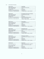
Appendix A: Node Properties
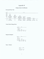
Appendix B: Runge-Kutta Co-efficient
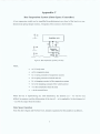
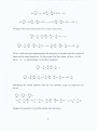
Appendix C: Bus Suspension System
Appendix D: SimDynamic Installation Instruction
Appendix E: SimDynamic Source Code (electronic format)
List of Figures
No.
Legend
Page
2.1
Animated hand for 5DT Glove..........................................................................
15
2.2
VIO I-Glasses pitching......................................................................................
15
2.3
VIO I-Glasses yawing.......................................................................................
15
2.4
Remote S&A and data transfer..........................................................................
26
2.5
Client-Site simulation with loaded applets.........................................................
26
2.6
Remote simulation and local visualization.........................................................
27
2.7
Web-enabling software model...........................................................................
28
2.8
Hardware and software layout...........................................................................
31
3.1
Node set window..............................................................................................
35
3.2
Model sheet window.........................................................................................
36
3.3
SimDynamic on-line help...................................................................................
37
3-4
Logical representation of a node.......................................................................
37
3-5
Node menu.......................................................................................................
38
3-6
Parameter dialog box for Discrete State Space....................................................
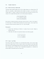
39
Row vector as parameter....................................................................................
40
3*8
Column vector as parameter..............................................................................
40
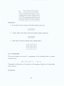
3-9
Matrix parameter...............................................................................................
41
310
Line drawing step 1...........................................................................................
43
Line drawing step 2...........................................................................................
^
3 12 Line drawing step 3............................................................................................
43
3-13 Line drawing step 4............................................................................................
43
314
Line menu.........................................................................................................
^
315
Branch line drawing step 1................................................................................
44
3-16 Branch line drawing step 2....................................................................................
44
3.17 Simulation parameters dialog box......................................................................
45
3.18
3D model editor window...................................................................................
47
3.19 Dialog box for 3D box......................................................................................
48
4.1
SimDynamic package hierarchy.........................................................................
49
4.2
Class hierarchy in UlPack package.....................................................................
50
43
Class hierarchy in NodePackpackage..................................................................
54
viii
4.4
Class hierarchy in Anim3D package..........................................................................
64
5.1
Backlash in gears...........................................................................................
92
5.2
Dead-band......................................................................................................
92
6.1
Step 1 for ODE model...................................................................................
114
6.2
Step 2 and 3 for ODE model...........................................................................
115
6.3
Completed ODE model...................................................................................
116
6.4
Graphical result for ODE model......................................................................
117
6.5
Numerical result for ODE model....................................................................
117
6.6
A simple pendulum........................................................................................
118
6.7
Pendulum model in SimDynamic....................................................................
119
6.8
Graphical result for pendulum model (rod length 1 meter)...............................
120
6.9
Graphical result for pendulum model (rod length 0.5 meter)............................
121
6.10
Pendulum 3D model.......................................................................................
123
6.11
3D animation for pendulum model..................................................................
123
6.12
A ball is thrown downward with velocityV0....................................................
124
6.13
Bouncing ball model in SimDynamic..............................................................
125
6.14
Graphical result for bouncing ball model (£ = 0.8)............................................
126
6.15
Graphical result for bouncing ball model (e = 1.0)............................................
126
6.16
3D animation for bouncing ball model............................................................
127
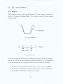
6.17
Bus suspension system (1/4 bus)....................................................................
128
6.18
Bus suspension model (open loop) in SimDynamic..........................................
129
6.19
Bus suspension model (closed loop) in SimDynamic......................................
130
6.20
Graphical result for bus suspension model (open loop)....................................
131
6.21
Graphical result for bus suspension model (closed loop)..................................
131
6.22
Discrete pulses applied to closed-loop bussuspension model............................
132
6.23
3D animation for bus suspension model...........................................................
133
ix
List of Tables
No.
Legend
Page
6.1 Numerical result for the Pendulum model (rod length 1 meter)..........................
120
6.2 Numerical result for the Pendulum model (rod length 0.5 meter)......................
121
6.3 Results for QDM model....................................................................................
136
x
Chapter One
1
Introduction
1.1
Virtual Reality
Virtual Reality (VR) is the simulation of a real or imagined environment that can be
experienced visually in the three dimensions o f width, height, and depth and that may
additionally provide an interactive experience visually in full real-time motion with
sound and possibly with tactile and other forms o f feedback. The simplest form of
virtual reality is a 3D image that can be explored interactively at a personal computer,
usually by manipulating keys or the mouse so that the content o f the image moves in
some direction or zooms in or out. This type o f experience is known as desktop VR or
non-immersive VR.
On the other hand, the strict definition of VR involves the sense of total immersion.
To experience a virtual reality, a user dons special gloves, earphones, and goggles, all
o f which receive their input from the VR system. In this way, at least three of the five
senses are controlled by the VR system. Therefore, the user is in computer-generated
3D, artistic renderings o f real or imagined spaces.
From these above definitions Virtual Reality can be divided into:
•
The simulation of real environments such as a manufacturing process or a
spaceship often with the purpose of training or education.
•
The development of an imagined environment, typically for a game or
educational adventure.
1.1.1
T ypes o f V R S ystem
VR systems can be classified based on the mode with which they interface to the user.
The most common modes used in VR systems are as follows:
a)
W indow on the W orld Systems (WoW)
In this system a conventional computer monitor is used to display the visual world.
This is sometimes called Desktop VR or a Window on the World (WoW). This
1
concept traces its lineage back through the entire history o f computer graphics. One
must look at the screen as a window through which one beholds a virtual world. It is
up to the computer graphics to make the picture in the window look real, sound real
and the object real.
b)
Video Mapping
Video Mapping can be considered as an extension of WoW approach. A video input
of the user’s silhouette is merged with a 2D computer graphic in a WoW system. So
the user watches a monitor that shows his body’s interaction with the virtual world.
c)
Immersive System
Immersion is a key issue in VR systems as it is central to the paradigm where the user
becomes a part of the simulated world. The ultimate VR systems completely immerse
the user’s personal viewpoint inside the virtual world. It has to meet four conditions:
(1) a head-mounted device (HMD) with a wide field of view; (2) tracking the position
and attitude of the user’s body; (3) transducers that interpret user’s natural behaviours,
and (4) negligible delays in the rate at which the virtual environment is updated in
response to user’s movements and actions.
d)
Telepresence
Telepresence is defined as the experience of presence in an environment by means of
a communication medium. In other words, it refers to the mediated perception o f an
environment. This environment can be either a temporarily or spatially distant real
environment or an animated but non-existent virtual world synthesized by a computer.
e)
Mixed Reality
Merging the telepresence and VR systems gives the Mixed Reality or Seamless
Simulation systems. Here the computer generated inputs are merged with telepresence
inputs and/ or the user’s view of the real world. For example a fighter pilot sees
computer generated maps and data displays inside his helmet visor or on cockpit
displays.
2
1.2
Simulation
A system is defined to be a collection of entities, e.g. people or machines that act and
interact together toward the accomplishment of some logical end. A model is a
simplified representation o f a system at some specific point in time and or space
intended to promote understanding o f the real system. Simulation is the discipline of
designing a model of an actual or theoretical physical system and manipulating the
model in such a way that it operates on time or space to compress it, thus enabling one
to perceive the interactions that would not otherwise be apparent because o f their
separation in time or space. It is a discipline for developing a level o f understanding
o f the interaction of the parts of a system, and of the system as a whole. And this level
o f understanding is seldom achievable via any other discipline. Simulations are
generally iterative in their development. One develops a model, simulates it, learns
from the simulation, revises the model, and continues the iterations until an adequate
level of understanding is developed.
1.2.1
Types o f Sim ulation M odels
a)
Static vs. Dynamic Simulation Models
Static models describe a system mathematically, in terms o f equations, where the
potential effect of each alternative is ascertained by a single computation o f the
equation. Static models ignore time-based variances. So they represent a system at a
particular point of time or a system in which time simply plays no role. Also, this type
of model does not take into account the synergy of the components o f a system, where
the actions of separate elements can have a different effect on the total system than
the sum of their individual effects would indicate.
On the other hand, a dynamic simulation model represents a system as it evolves over
time. It is a representation o f the dynamic or time-based behaviour o f a system. While
a static model involves a single computation of an equation, dynamic modelling is
iterative. A dynamic model constantly re-computes its equations as time changes.
Dynamic modelling can predict the outcomes o f possible courses o f action and can
account for the effects of variances or randomness. One cannot control the occurrence
3
of random events, but can use dynamic modelling to predict the likelihood and
consequences o f their occurring.
b)
Deterministic vs. Stochastic Simulation Models
A deterministic model can be identified as a model that does not contain any
probabilistic (i.e. random) components. In such models output is determined once the
set of input quantities and relationships in the model have been specified.
On the other hand, many systems must be modelled as having at least some random
input components, and these give rise to stochastic simulation models. Most queuing
and inventory systems are modelled stochastically, and these models produce output
that is itself random.
c)
Continuous vs. Discrete-Event Simulation Models
Discrete event simulation concerns the modelling o f a system as it evolves over time
by a representation in which the state variables change instantaneously at separate
points in time. These points in time are the ones at which an event occurs, where an
event is identified as an instantaneous occurrence that may change the state of the
system.
Continuous simulation models concern the modelling over time of a system by a
representation in which the state variables change continuously with respect to time.
Typically, continuous simulation models involve differential equations that give
relationships for the rates o f change of the state variables with time. If the differential
equations are particularly simple, they can be solved analytically to give the values of
the state variables for all values of time as a function o f the values o f the state
variables at time 0. For most continuous models analytic solutions are not possible,
however, and numerical-analysis techniques, e.g. Runge-Kutta integration, are used to
integrate the differential equations numerically, given specific values for the state
variables at time 0.
4
1.3
World Wide Web
The Internet is a collection o f interconnected computer networks operating under a
common communications protocol. The World Wide Web (WWW), currently the
fastest growing segment o f the Internet, is a collection of electronic documents called
pages, which reside on computers called WWW servers. These documents contain a
combination of text, images, audio and video. The pages on the Internet are public
and anyone can generate a page and put it on a WWW server. The pages and the
associated files must meet a standard protocol.
The text portions o f the document are written in a mark-up language called HTML
(Hypertext Markup Language) [1]. Hypertext is text with links such that the user can
follow a non-linear path through a document or set o f documents. The unique
characteristics of WWW hypertext documents is that the links can point to positions
in the same document, positions in the other documents on the same server, or to
WWW pages on any server anywhere on the Internet. They can also link to images,
audio or video. The links are indicated by highlighted text and the link is established
by pointing and clicking on the highlighted text.
A person, group or organization creates a page because they have certain information,
which they wish to make available to other people. Usually this information is related
to and hence references information others have decided to make available. Hence the
pages point to one another and, as they multiply, form a web. Thus the WWW is a
body and organization of information, which has no top down structure but is
organized in a completely bottom up fashion by the individuals creating the individual
pages.
The addresses o f the pages are called URL’s (Universal Resource Locators) [1] and
there is a standard communications protocol (HTTP) [1] for requesting and obtaining
any public Web page from any public server. The user o f the Web operates on a
client, a workstation or PC running a Windows, UNIX, Macintosh or OS/2 operating
system. The client has software, called a browser, which enables it to request a page
from the server and process the HTML file presenting the processed material to the
user.
5
Therefore, the Internet and the WWW hold tremendous potential for the
communication and the general distribution of information within groups with a
common professional interest.
1.4
Web - based Simulation
In recent years the Internet in general, and World Wide Web (WWW or Web) in
particular, have grown rapidly as dissemination tools for different kinds of
information resources. Frequently, the Web is used for deployment o f educational and
commercial material. Educators are using the Web to post course notes, syllabi,
homework assignments, and even exams and quizzes. Companies are using the Web
for advertising, publicity, and to sell products. Through JAVA [2], an object oriented
programming language, people can also customize WWW based computational
programs as they would with traditional non-Internet based programs, and there is a
growing interest in using the Web as a new platform for computer programs. The
disciplines concerned with computer simulation are no exception to this phenomenon;
the concept of web-based simulation has been introduced and is currently the subject
of much interest to both simulation researchers and simulation practitioners. Webbased simulation is an attempt to exploit Web technology to support the future of
computer simulation. Apart from providing other services, the World Wide Web is
being looked upon as an environment for hosting modelling and simulation
applications. Existing computer simulation support is either language-based or a
library approach. In either case, they suffer from lack o f portability to other
environments. Also markets in educational software are small. There are thus little
commercial interests in the production of simulation software for the educational
market. Any simulation software, which is produced is aimed at the industrial market
and is often too expensive for the educational purchaser. Moreover the demand for
consulting in modelling and simulation has grown faster than the consulting
companies can offer. Use o f the Internet and its supporting tools such as the virtual
environment and the interactive distributed simulation has the potential to overcome
these factors limiting the wider use of simulation. The web’s ability to service large
and diverse audiences allows the simulation community to legitimately provide
models and simulations as end products. Recent advances in web technology have
6
made the web a viable mechanism for performing, publishing, and distributing
simulation.
1.5
Advantages and Disadvantages of Web - based Simulation
A Web-based simulation program provides several beneficial features that are lacking
in available non Web-based packages. These features include wide availability,
controlled access, user friendliness and efficient maintenance etc. On the other hand,
simulation over the WWW does have a few potential drawbacks. These advantages
and disadvantages should be considered when deciding which simulation package
best meets a user’s needs. This section discusses some of these features provided by a
Web-based simulation program.
Wide Availability: In case o f non Web-based simulation software, a change in
platform (whether change in operating system or computer hardware) forces the
recompilation o f the simulation model (programme). Utilizing this type of package
requires access to a computer containing the proper simulation software, as well as an
appropriately compiled copy of the model source. The portability o f a Web-based
model onto various platforms enables the user to access and run the model from wide
spread locations. There is no need to transport hardware or software to these sites or
recompile the code. Moreover Internet is usually available twenty-four hours a day,
access to the simulation software is not limited by time constraints. So the users can
work within their own time schedule.
Controlled Access: With non Web-based package, user can access the model and
software directly from the computer on which the model is running. There is every
possibility of inadvertent modification to the model whenever the user has free access
to the complete source code o f the model and the software. On the other hand, Webbased simulation software and models can be protected from unauthorized
modifications by imposing password and time limit restrictions on either the
simulation package or the entire site.
User Friendliness: Most of the non Web-based packages need proper installation of
the software and working knowledge of the operating commands. Web-based
simulation software and models developed with Java require only a Java-compatible
7
Web browser for viewing. Such browsers like Internet Explorer or Netscape are
readily available, easy to install and already installed on many computer systems.
Since many users are familiar with navigating Web browsers, the total software
learning curve using a model is a minimal.
Furthermore, web-based simulation environment provides the same user interface for
all users. Although some non Web-based groupware (computer based systems, that
support groups o f people engaged in a common task) simulation packages provide a
common interface to a shared environment, these software solutions have two main
shortcomings. Firstly, most o f these packages are system dependent, all participants in
a project are bound to use a system that is supported by the groupware application. All
participants must own the software to use. The second disadvantage o f any existing
groupware is the lack of simulation awareness. It will support the communication of
project participants, exchange o f files, but it is still detached from the actual
application, simulation.
Efficient Maintenance: Web-based simulation programmes enable reliable version
control and frequent model modifications. In most o f the traditional groupware
packages, modifications can be tedious and time consuming. Users must be made
aware of the need for and existence o f an updated model. Then update must either be
made on each copy o f the model, or the new model should be delivered to each
participant and the old one deleted. In Web-based modelling there is only one model
at a particular time that is residing on the Web-server. The existence o f a single
working model enables modifications with smaller degree o f error. Additionally, the
model creator has access through the Internet to the model’s source code on the
serving computer. This allows that person to access the server from distant site. Also
the most up-to-date version o f the model is instantly available through the server to all
authorized users, regardless of the physical location.
Despite these advantages of WWW based simulation, traditional simulation packages
may be useful over Web-based simulation in many cases. Traditional packages are
specialized to idiosyncrasies of a single platform, making maximum use o f its
capabilities. This may increase efficiency o f simulation runs. Loading times for
traditional programmes are dependent on the computer and not on the current volume
8
of Internet usage. During heavy Internet traffic, models with complex or extensive
amounts of code may initially take large amount of time to download.
1.6
Objective of the Project
The objective of the project is to develop a virtual reality based simulation software
(SimDynamic). Proposed simulation engine will be powerful enough to handle both
discrete event simulation and dynamic system simulation. In case of dynamic
systems, it will support linear and non-linear systems, modelled in continuous time,
sampled time, or a hybrid of the two. Systems can also be multi-rate, i.e. have
different parts that are sampled or updated at different rates. Java will be used to
develop the package, so it will be accessible over the Internet. Using any java enabled
browser, a simulation problem can be modelled in SimDynamic, and such java-based
models allow the user the same degree of interactive, multimedia capability, as do
non-Internet based programs. SimDynamic can also be used as a non Web-based
application on a PC. For modeling, the package provides a graphical user interface
(GUI) for building models as block diagrams, using click-and-drag mouse operations.
After a model has been defined, it can be simulated, using a choice o f integration
methods. Finally the results of the simulation can be viewed as both graphical and
numerical output as well as 3D animation.
This thesis is organized into seven chapters and five appendices. A literature review is
presented in chapter two. It mainly covers previous work carried out by different
researchers in the area of virtual reality & simulation, dynamic system simulation and
Web-based simulation. Chapter three introduces SimDynamic from a user’s point of
view. This chapter provides all the information needed to build a model, execute and
handle the GUI. Chapter four describes the architectural design o f the software.
Chapter five can be considered as an extension of chapter four, but they can never be
merged. This chapter describes the functional ability o f the core components of
SimDynamic. Chapter six focuses on the application o f the software. Some real world
systems have been modelled using SimDynamic and this chapter demonstrates the
results obtained from the simulation. Finally chapter seven outlines the conclusions
and the recommendations for further work.
9
Chapter Two
2
Literature Survey
2.1
Virtual Reality and Simulation
The popular media representation o f Virtual Reality has tended to emphasize the
entertainment aspects of the technology. But a virtual environment can be used as an
effective tool for simulation, training and education. Barnes [3] provides an awareness
of Virtual Reality with respect to simulation. The newer workstations and PCs
provide performance that support VR at an affordable price. VR software is now
available to run on these platforms. Some o f this software comes with simulation
engines that support simulation modelling and analysis. The paper describes the tools
and methods that are particular to VR and illustrates how these are being applied to
simulation. The applications presented in the paper focus on virtual manufacturing
and the VR world animated with behaviour controlled by a simulation engine, which
uses simulated behaviour rules and model data.
Sikorsky Aircraft Co. USA and British Aerospace, UK, used simulation software like
QUEST [4], IGRIP [5] to recreate the actual manufacturing process. Visualization
allows the user to assemble the components in a Virtual Manufacturing cell. This
could be by utilizing the 3D models o f the part designs using popular CAD packages,
such as Unigraphics, Intergraph, CATIA or Pro/ ENGINEER to visualize how the
components relate to each other. In the model, the user can manipulate and view each
of the components to develop a manufacturing approach. Virtual Manufacturing
modelling allows the user to introduce the engineering design to the processes that
will be used to create the actual part, assembly, or installation. The tool design is
imported to the model, combined with the part and dynamic representations o f the
machines that will produce the part. Machines are programmed to operate identically
in the virtual environment as they would in the real environment. Design problems
such as collisions, clearances, missing manufacturing features, fit, and manufacturing
sequence issues are quickly identified. Manufacturing and design concepts are easily
developed with minimal cost to the program. The ability to insert people in the
environment and analyze their activities minimizes ergonomic problems. Factory
10
modeling allows engineers to predict the cost and schedule impact of potential design
or process changes. The information provided by the simulation enables “what i f ’
analysis. The model provides support personnel with a tool to optimize the
manufacturing, try new concepts without disrupting manufacturing and predict
changes due to load variations. The three common elements in the evolution o f a
product are cost, schedule, and information. Virtual Manufacturing allows engineers,
designers, suppliers, and others to understand the cost and schedule impact of
decisions and to consolidate processes. Overhead costs are addressed by improving
schedule performance. The amount of time it takes to design, plan, tool and
manufacture a product directly impacts overhead costs. A reduction in time it takes to
get a product to market equates to a return on investment (ROI) improvement.
General Dynamics Electrical Boat Division for the US navy developed prototypes o f a
nuclear attack submarine, which was designed, evaluated and optimized in a virtual
environment. Electric Boat demonstrated the feasibility o f state-of-the-art simulationbased design (SBD). The objective was to implement an accurate, efficient, and
dynamic environment for design, rapid prototyping, concurrent product and process
development, mission planning, operation maintenance, and training. By simulating
the kinematic, dynamic, mechanical, and other characteristics o f the submarine, its
components and subsystems, engineers can create a multi-disciplinary environment in
which to evaluate a wide range o f parameters and optimize the design based on the
results. Electric Boat selected simulation software ENVISION [5] to visualize design
concepts and integrate components and subsystems. Virtual engineering allows the
parties involved with design, manufacturing, operations, and maintenance to jointly
contribute to the design process early in the cycle. Electric Boat engineers often
experience communication difficulties when trying to describe innovative ideas to
people not trained in their particular discipline. The physically accurate 3D models
simulated in ENVISION help engineers and technicians from various disciplines to
comprehend new ideas and concepts. In addition, virtual reality technologies such as
immersion enable engineers and their naval customers to “walkthrough” the model
with visual feedback. Immersion provides for evaluation other design criteria, such as
ergonomics, before a design is built.
11
The most recent development in the use of Virtual Manufacturing software is the use
of the Virtual Collaborative Engineering (VCE) environment that links multiple users
at multiple locations to discuss, analyze, and review simulations over a wide area
network. VCE users interactively evaluate design concepts, manufacturing tooling,
processes, and factory layouts — even at geographically remote locations. Any VCE
user can assume control o f a simulation, make changes, or view changes made by
others on the VCE network. Engineers, manufacturing personnel, system operators, or
other users interact within the same simulation, creating a “virtual conference room”
for design discussion, evaluation, and approval.
Jones, et al [6] describe a software engineering project, initiated to explore how
virtual reality might impact simulations and to gain insight into bringing the
technology
to
commercially
available
simulation
software
packages.
AutoSimulations, Inc. [7] provided licenses and source code to their AutoMod and
Auto View simulation software for the project. Human Interface Technology
Laboratory (HITL), University o f Washington, provided the virtual interface
hardware, software, and necessary software engineering support. The VR software
used in the project was actually two components o f a suite of virtual reality software
developed at HITL: VEOS (Virtual Environment Operation System), a distributed
database and data transport package created for research and rapid prototyping of
virtual environments, and Image Library created for research into VR related
rendering issues. The objective o f the project was to create virtual factory that would
allow a user to experience a three-dimensional “playback” of a simulation. The user
could move around in the factory but would not be able to make changes to the
simulation other than starting and stopping simulation time. The user has to don a
head-mounted display (HMD), which conveys visual information to each eye via two
separate video screens. A tracking device allows the VR system to monitor the user’s
head position and orientation at all times. A computer with special graphics hardware
continually renders for each eye a perspective image o f the virtual environment from
the eye’s instantaneous viewpoint, based on the user’s head location. When the user
sees these images through the HMD, the images fuse to form a single, stereoscopic
view of the virtual environment. The user can turn in any direction and see objects in
the environment in the same way that one can turn one’s head and discover what is
behind him. Additionally, the user can move or ‘fly’ through the environment by
12
means of a hand-held joystick. For testing the project, a simulation o f the wheel
assembly area of Derby Cycle, a producer of recreational and sport bicycles in Kent,
Washington, was constructed. Production and manufacturing personnel were used as
subjects for evaluating the interface. Five subjects from Derby Cycle participated and
were shown either the virtual environment or the Auto View animation on a computer
screen. Subjects were asked questions to determine their understanding o f the virtual
factory and follow-up written survey and group discussion was also conducted. One
notable conclusion from the survey and group discussion was that the virtual factory
captured the imagination o f the Derby employees. Participants who viewed the virtual
factory were much more talkative and involved in the exploration of the simulation
than the subjects who experienced Auto View.
Marcedie, et al [8] cite many recent examples of virtual environments that can be
used as effective tool for training and education. The paper also introduces a novel
technology to support distributed virtual environment. Existing VR systems lack
distributed access; they have no central computer for event scheduling or conflict
resolution. Computers (or autonomous simulation nodes) on which the system is
running are responsible for maintaining the state of one or more simulation entities.
Simulation nodes communicate primarily changes of their state and they are
responsible for determining what is perceived. Such a system suffers from high
communication volume. The proposed new architecture overcomes these problems of
existing systems by taking advantages of the features of the object oriented
programming paradigm.
As an object oriented simulation system, the basic system elements in the proposed
architecture are objects located at different machines. These machines are called
nodes and are connected by the network. At any single node, there are three major
objects.
a) The message handling object controls the messages passed between local
objects and the network. Unlike current approaches, which broadcast all
messages on the network, it uses both broadcast and point-to-point approaches
to send the messages to keep the number of redundant messages as low as
possible.
13
b) With update messages, the situation delay object is used to display the states
o f all entity objects distributed at the nodes. The display updates with
simulation time advance.
c) The simulation object at a node contains a series o f entity objects, which
represent physical entities in the real world. It is responsible for creating and
deleting its derivative entity objects. It transfers the messages from its
derivative entity objects to its other derivative entity objects or to the other
objects located at other nodes via the computer network. Another important
task of the simulation object is to control the local simulation time advance.
In short, this prototype object oriented architecture is composed of non-autonomous
simulation nodes. With an appropriate user interface, the nodes appear as an
integrated virtual environment to the user. Simulation entities are modelled as
simulation entity objects, which are distributed at different nodes and are migrated
dynamically between the nodes during the simulation run. This mechanism o f object
management presents the possibility o f reducing message volume. Communication
efficiency can therefore be improved by two measures. One is to dynamically group
closely related simulation entity objects to a specific node. Alternatively, a point-topoint communication approach can be used instead of broadcast.
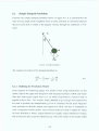
Grant and Lai [9] present SMART, a simulation modelling tool that provides a virtual
reality interface for building graphical simulation models. The simulation models,
comprised of nodes and arcs, are constructed in three dimensions. As the user builds a
model, he may immerse himself in it using virtual reality hardware and software tools
and take advantage of the three-dimensional environment provided by SMART. It has
been developed to explore the use of virtual reality in building simulation models, and
it serves as a prototype for testing the feasibility o f creating a virtual reality simulation
modeling software system on a relatively low cost personal computer. SMART offers
three-dimensional interface using virtual reality hardware, which includes an
electronic glove and head-mounted display. The specific hardware is the 5DT Glove
[10] and VIO I-Glasses [11] respectively.
14
The 5DT Glove is used by SMART as the primary manual input device. The
electronic glove is plugged into a PC’s serial port. The configuration parameters of
the 5DT Glove such as the bending angle of each finger and, pitch and roll o f the
wrist are constantly sampled by the PC’s serial connection and sent to SMART for
processing. The user controls SMART using a set o f gestures to cause actions to be
taken when building simulation models. When a recognizable gesture is detected,
SMART responds with the appropriate action and provides audio feedback
confirming the action. The glove’s configuration and its relative position in the virtual
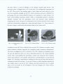
world are continuously animated by a robot-like hand (figure 2.1). Every motion of
the user’s fingers is reflected by the animated hand in the virtual world.
Fig 2.1: Animated hand for 5DT
Glove
Fig 2.2: VIO I-Glasses pitching
Fig 2.3: VIO I-Glasses yawing
In addition to the 5DT Glove, SMART also uses the VIO I-Glasses as another virtual
reality hardware interface especially for simulation model immersion enhancement.
The device is plugged into a PC’s serial port. The VIO I-Glasses are designed to give
the user the impression that he or she is physically present in the virtual modeling
world. This is accomplished by providing a virtual view using the VIO I-Glasses,
which reacts directly to two primary head motions: pitching (figure 2.2) and yawing
(figure 2.3). Pitching is equivalent to nodding the head up and down and yawing is
swinging the head left and right. To use the I-Glasses to build simulation models, the
user simply needs to put on the VIO I-Glasses and look around the way he usually
does in the real world. As the orientation of the user changes, the virtual world is
rendered accordingly.
15
2.2
Dynamic System Simulation
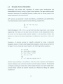
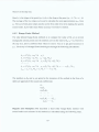
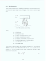
Kimbrough [12] provides APL algorithms for control system development and
demonstrates their use by solving a typical control problem. The paper outlines useful
numerical techniques for simulating dynamic systems and for solving some o f the
central equations o f the control theory.
APL functions are presented to check observability, controllability and stabilizability
of a linear dynamic system expressed in the following standard form,
Ax + Bu + D(x,u,t)v
dt
y-C x
— =
where the shapes of A, B, C, D, x, y, u and v are (n,n), (n,p), (n,q), (m,n), n, m, p and q
respectively. The vector x is the state vector, the vector y is the measurement vector,
the vector u is the linear control, and the variable v is the non-linear control. The
matrices A, B and
C
are time invariant but D is allowed to vary with x, u and t, the
time.
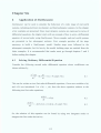
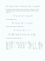
Simulation of dynamic systems is typically conducted by using a numerical
integration routine. A fourth-order Runge-Kutta integration routine is also provided in
the paper. This is a fixed step routine based on the following familiar equations,
K = f{y ,t)h
K - f ( y + 0.5k0,t + 0.5h)h
K = f ( y + 0.5kl9t + 0.5h)h
¿3
= f ( y + k2,t + h)h
and
y n+x = y " +( kQ+ k 3) / 6 + (kl +k2)/ 3
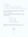
Besides using simulation it is possible to study the system response using frequency
domain techniques such as Fourier transform and the Laplace transform. Fundamental
to frequency techniques is the notion o f the transfer function. For multi-variable timeinvariant linear systems the transfer functions are obtained by taking the Laplace
transform of
16
— = Ax + Bu
dt
y-Cx
which yields,
y = C ( s I - A ) - ]Bu = H(s) u.
An APL function is also provided to generate Hfs).
All the algorithms presented in the paper can analyze, with reasonable response,
systems with up to 40 state variables while running on a mainframe and systems with
up to 20 state variables while running on a microcomputer. This capacity is sufficient
for many “real world” control problems and is more than enough for exploring the
features of control engineering.
Schmid [13] presents CADACS-PC Real Time Toolbox, an open software
implementation of the KEDDC [14] real-time suite, which runs on personal computer
and provides special real-time environments for developing microprocessor based
industrial control devices. Such control devices can be connected directly to the plant
to be controlled and support on-line identification o f the plant dynamics, as well as
evaluation of prototype control systems. The proposed software frame is independent
of the hardware and operating system, quite simple and also meets the requirements
for a real time control environment, such as monitoring, supervisory control or
scheduling etc. Although such a frame is contained in the real time suite of the
KEDDC system, the contribution focuses to the implementation o f the real time suite
on PC-based systems, where the entire power o f KEDDC is packed into one low-cost
and portable system, which can be taken to the plant to be analysed and controlled.
CADACS-PC supports a wide variety of control engineering methods. It offers tools
for the systematic design strategies and high-accuracy numerical solutions. In addition
to modem analysis and design concepts, classical methods are also implemented and
may be used in combination with modem control techniques. CADACS application
environment consists of several components and the most important components
consist of a group o f interactive programs for the management o f dynamic systems,
systems analysis, controller synthesis, simulation and signal processing. A unified
database for system models allows a smooth exchange o f data between the different
programs and between different groups o f a development or research project. Due to
17
the wide range of methods, the system may be used for the task o f industrial planning
o f plants, as well as for the subsequent analysis o f measured data; also for the
modeling of dynamic systems and for the design o f control systems. The multi
purpose real-time suite has highly modular structure and provides a high degree of
portability, which results from an interface o f CAD ACS to the operating system and
to hardware-dependent functions. Some basic routines build an interface to the world
outside of the programs and modules. The user can both monitor and store the real
time behavior o f any external or internal signal. At the same time or at a later date
s/he can evaluate and present results.
Fishwick [15] develops SimPack, a collection o f C and C++ libraries and executable
programs for computer simulation. The purpose o f the SimPack toolkit is to provide
the user with a set of utilities that illustrate the basics o f building a working
simulation from model description. Special purpose simulation programming
languages can be easily constructed using language translation software with the
SimPack utilities, which act as the “assembly language”.
Most of the existing simulation packages cover one o f two areas: discrete event or
continuous. Some available software can perform both types o f simulation; however,
bulk support is usually available in only one form. SimPack has the ability to
overcome this problem. It is designed
•
To support the variety o f available model types.
•
To create template algorithms for many cases.
•
To avoid learning a special language syntax.
•
To illustrate the relationship between event and process oriented discrete event
simulation.
SimPack supports simulation development for a wide variety o f modeling types
including the following:
•
D eclarative Models: An emphasis on explicit state-to-state changes as found
in finite state automata and Markov models.
18
VI ’ '
1 ‘ !
M
'
:
» *
t r. '
'
j• ! sv . . • » }Si .....
Functional Models: A focus on “function” or “procedure” as in queuing
.
•
•' .
-y
-n
.■-• 7 , r ,
'* :
W . ; j •. -.'V-';:
networks, block models, pulse processes and stochastic Petri nets.
t r.
!
or network to solve combined' simulation problems at multiple abstraction
levels.
•
1
Constraint Models: The constraint part o f SimPack i n c h e s capabilities for
modeling 1) difference equation systems, 2) differential equation systems, and
3) delay differential equation systems. In most cases, the most uniform method
of simulation is to convert the equation(s) into first order form and then to
simulate the system by updating the state vector.
Otter [16] presents DSSIM, a general-purpose simulation for dynamic systems.
DSSIM is a part of ANDECS [17] environment, which is a powerful and flexible
software package for the analysis and design o f controlled dynamic systems.
ANDECS consists o f a wide collection o f methods, such as basic mathematical
methods like matrix computation, interpolation o f signals or root finding o f nonlinear
functions. Analysis and design methods for linear dynamic systems like linear
simulation, calculation of poles and zeros, pole placement. Standard diagrams like 2D
line, Bode, Nyquist and root locus diagrams. Special diagrams like parallel
coordinates to visualize optimization criteria. DSSIM is the run time environment of
ANDECS to simulate dynamic systems. It uses following well-tested numerical
integration routines,
•
DEABM - Multi-step solver o f Shampine/Watts for non-stiff and moderately
stiff ODEs.
•
LSODE - Multi-step solver o f Hindmarsh for stiff and non-stiff ODEs.
•
LSODAR -
Multi-step solver o f Petzold/Hindmarsh, which switches
automatically between a non-stiff and a stiff integration algorithm along the
solution. LSODAR also provides a root finder.
•
RK45/78 - Runge-Kutta-Fehlberg solvers o f Kraft/Fuhrer o f fixed orders 5
and 8 with variable step-size using the Prince-Dormand coefficients.
19
•
GRK4T - A stable linearly implicit Rosenbrock type single-step solver o f
fixed order 4 for stiff and oscillating ODEs of Arnold.
•
DASSL/RT - Multi-step solvers of Petzold for DAEs and for DAEs with root
finder.
•
ODASSL/RT - Multi-step solvers of Führer based on DASSL/RT o f Petzold
for ODAEs and for ODAEs with root finder.
•
MEXX - Extrapolation solvers o f Lubich for a restricted class o f index-2
ODAEs.
There are a wide variety o f options available to define a simulation experiment. The
result of simulation experiment is a set of computed signals, which are automatically
stored on a database and visualized with any available graphics module. All input data
of an experiment, e.g. integration method or length o f communication interval, are
stored on database as well. Therefore every simulation run is completely documented
and reproducible.
Elmqvist, et al [18] present a new methodology for object-oriented modeling of
hybrid systems. Hybrid models contain both continuous and discrete parts. In
simulation programs, the continuous parts are described by sets o f differential
equations and algebraic equations in either explicit form or implicit form. The discrete
parts are expressed with event descriptions. Object-oriented programming has evolved
to support the reuse o f software components. This programming paradigm was first
developed in the context o f discrete-event simulation and carried over to continuous
systems modeling. Dymola [19], an object oriented modeling language, for
continuous systems, was designed for this purpose. It represented an important step
forward towards the reuse o f continuous systems models in a truly environmentindependent fashion. A continuous system modeling methodology that doesn’t allow
for descriptions o f discontinuities is not generally useful since all but the most trivial
engineering models o f dynamic systems contain some sort o f discontinuities. The
paper discusses an extension o f Dymola language definition to allow descriptions o f
models of dynamic systems with discontinuous behavior in a truly reusable objectoriented fashion.
20
There are some packages like VisSim, Simulink, Maple available in the market for
dynamic system simulation. Both VisSim and Simulink support modelling and
simulation of complex continuous non-linear dynamic systems. They combine an
intuitive drag and drop block diagram interface with powerful simulation engine that
provides fast and accurate solutions for linear, non-linear continuous time, discrete
time, time varying and hybrid system designs. The visual block diagram interface
offers a simple method for constructing, modifying and maintaining system models.
2.3
Web Based Simulation
Research on distributed interactive simulation; its feasibility and application began in
the mid 1970’s. In the 1980’s Miller and Thorpe [20] in partnership, with the US
Army created SIMulation NETworking (SIMNET), a networked system o f computers
running a single simulation programme. SIMNET was sponsored by ARP A (then
called DARPA), and it was an attempt to make the use o f simulators and simulation
techniques
more
feasible
for military defense
operations.
This programme
demonstrated the feasibility of linking together hundreds or thousands o f simulators
(representing tanks, infantry fighting vehicles, helicopters, fixed-wing aircraft etc.) to
create a consistent, virtual world in which all participants experience a coherent,
logical sequence o f events. In SIMNET, standard Ethernet networks were used for all
local area network (LAN) connections. Ethernet bridges were used via 56 kbps dial
up links to connect two or more LANs to form a single, logical Ethernet LAN. The
success of SIMNET resulted in a standardized simulation networking protocol,
Distributed Interactive Simulation (DIS). After several revisions and extensions o f the
SIMNET protocols, in March 1993, the first standards were formally approved [21].
DIS is a protocol for communicating position and other information to other entities
in a simulated battlefield. Each entity can see each other and interact in a virtual
environment. Although DIS began in the military environment, it is now being used
increasingly often in non-military applications such as air traffic control, intelligent
vehicle highway systems, and interactive multi-user computer games.
Neilson and Thomas [22] discuss the use o f the Interact Simulation Environment
(ISE), created as an aid to teaching engineering students. At the heart o f ISE is an
interactive environment in which a simulation can be integrated into a distributed
21
hypermedia system. Such integration permits a simulation to be treated as just another
medium of expression, equivalent to media such as the text, graphics and sound. It
allows a simulation to be treated as a resource along with other resources such as
video clips, graphics etc. It allows a simulation to be used not only with a wide variety
of supporting material but also in a wide variety o f contexts thus increasing the
usefulness of the simulation as a learning resource. Some additional contexts are: use
as a stand-alone simulation in a lecture with no supporting hyper textual material; use
within a laboratory class for demonstrations, structured enquiries, open ended
enquiries and projects; use in studies o f parametric changes; use in optimisation of
system parameters and in tests o f sensitivity; giving students experience of modelling
systems; input and output datasets can be provided from which students have to
deduce the model which gave rise to that output; given a specification students could
be asked to provide a model to achieve that specification. Students could be required
to produce hypertext reports o f their work, which include links to the simulation in
various states. Because o f differences in student’s background computer knowledge,
the ISE is set up to utilize simulation as a modelling tool without requiring the student
to interact with the actual simulation interface.
Cole and Tooker [23] have developed WWW-based physics tutorials to assist physics
students. Making these simulation models available over the WWW greatly expands
the range of possible access locations. Like ISE, the physics tutorials allow students to
see interesting cases o f a given simulation model without requiring prior knowledge
of the parameters defining these cases or o f the background programming languages
involved. Additionally, the use of familiar WWW browsers such as Netscape virtually
eliminates the amount o f time necessary for distributing and learning viewing
software. The tutorials use Apple’s OpenDoc Frameworks to provide a basic
simulation environment. OpenDoc is based on the idea o f container documents and
components that act on documents. Using OpenDoc one can build software
components, in this case physics simulation models. It can be then embedded in
container documents such as a web browser document or word processing document
depending upon the need of the user. The main attribute o f the environment is its
extensibility. One can extend the power o f the environment by adding parts. This
extensibility means it is functional for a broad spectrum o f users.
22
Fishwick [24] focuses on three important aspects o f simulation that might be affected
by incorporating it in the Web:
a) Education and training: Using the WWW for education and training allows
and encourages the reuse of knowledge by providing us with effectively
infinite storage, unlike the CD-ROM and diskettes. The storage is on the
Internet and not limited to one’s own machine. Therefore simulation packages,
which include help text and information about the pieces o f the model, can
have these pieces on the Web so that they do not require local storage. It is not
necessary for a company to re-build every piece o f information about a
manufacturing process, for instance, from scratch. Information on automated
guided vehicles (AVGs), machine specifications, and automated conveyance
mechanisms may already be located somewhere on the Web. These sorts of
devices are common in simulation programs built for manufacturing analysis.
The Web encourages this sort of global view with a reuse of knowledge and
information. The most profound affect the Web may have on the method of
teaching simulation lies with the use of multimedia. The Web encourages
distance learning more so than the typical simulation textbook. On any web
page it is possible to include images and video o f the instructors along with
synchronized slides or overheads. This immerse the student in a synthetic
learning environment that is more congenial than one they would get simply
by reading a book or watching a videotape.
b) Publications: Additionally, he discusses the timesaving aspects of using
WWW tools in reading publishing research articles. The WWW is valuable in
all stages o f producing an article, from accessing documents via electronic
database or URLs cited in bibliographies, to transmitting electronic copies of
the publication to reviewers and for the final publication. Simulation models
can be embedded in web documents that can contain videos, images, and
audio in addition to the usual text that traditional documents contain.
c) Simulation Programmes: Typically scripting languages such as Perl, Java
Script, or Java are used to build the model. The paper gives an example o f a
23
simulation model using Perl script to demonstrate current workstation
resource, queuing sizes based on user input gathered through an HTML form.
Besides the value of simulation in aiding understanding, Fish wick discusses
the possibilities o f WWW based simulation or simulation interfaces for multi
user situations such as multi-user dungeons (MUD), where users typically co
operate to reach a solution, and DIS discussed earlier.
SimKit, created by Buss and Stork [25] is a set o f Java classes for creating discrete
event simulation models. They use the event graph design approach to build models.
SimKit models, particularly geared to military applications,
can easily be
implemented as applets and executed in a web browser. The main simulation
facilitating package, JavaSim, is designed to allow for expansion in order to
accommodate frameworks for various types of simulations. JavaSim makes extensive
use of Java interfaces, which add defined behaviours to identified classes without
imposing the hierarchical structure o f class inheritance. This structure allows a
modeller to add customized tools into SimKit without making changes to JavaSim.
SimKit permits user interaction through a detailed, model entry form. Additionally,
SimKit is combined with a Java based graphic package designed by Leigh
Brookshaw, to allow a useful output o f statistics and graphs.
Miller, et al [26] present JSIM, a java-based simulation and animation environment. It
demonstrates WWW-based simulation through a unique combination of java applets
and query driven databases. JSIM provides the user with a simulation and animation
environment in which she/he can build simulation, execute the models, watch the
animation of a static design diagram, embellish the animation with special icons, and
generate statistics. A model is constructed by building a graph with nodes and edges.
Using the built in features of JSIM, the design diagram may be animated when the
simulation is run. For the purpose of storing and retrieving simulation models and
results, JSIM incorporates database connectivity with simulation classes. When a user
queries a simulation system, the system first tries to locate the required information in
the database, since it might have stored as the result o f an earlier model execution. If
the required data is present, it is simply retrieved and presented to the user. If it is not
present, the system instantiates the relevant model, executes it and shows the result of
the execution to the user.
24
SimJava, presented by McNab and Howell [27] is a process based discrete event
simulation package for building working models o f complex systems, with animation
facilities. It is actually a collection of three packages, simjava, simanim and simdiag.
simjava is a package for building stand alone text only java simulations, which
produce a trace file as the output by default, simanim is tightly integrated with the text
only simulation package, and provides skeleton applet for easily building a
visualisation o f a simulation, simdiag is a collection o f JavaBeans based classes for
displaying simulation results. A SimJava simulation model is a collection o f entities
(from the Sim_entity class) each running in its own thread within Java Virtual
Machine (JVM). These entities are connected together by ports (from the Sim_port
class) and can communicate with each other by sending and receiving event (from the
Sim_event class) objects. A central system class, Sim_system, controls all the threads,
advances the simulation time and delivers the events. The progress o f the simulation
is recorded through trace messages produced by the entities and saved in a file.
Utilizing the Remote Method Invocation (RMI) facilities of Java, Page, Moose and
Griffin [28] extends the SimJava (as described earlier) simulation package to enable
the construction of distributed, web-based simulation. In the Java distributed object
model, a remote object is one whose methods can be invoked from another JVM,
possibly on different hosts. An object o f this type is described by one or more remote
interfaces, which are Java interfaces that declare the methods o f the remote object. A
client can call a remote object in a server, and that server can also be a client o f other
remote objects. To add the RMI capabilities to SimJava, a simple master-slave
architecture has been designed. In this architecture, a master server is one that
encapsulates the central system class (Sim_system) and this class co-ordinates the
activities of objects (Sim_entities) that are distributed across the network. Given this
architecture, remote interfaces must be constructed for the Sim_system, Sim_entity,
Sim_port and Sim_event classes. To illustrate the concept o f the architecture the
paper also provides a self-explanatory example.
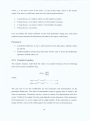
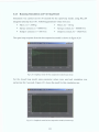
Lorenz,
et al [29]
describe three basic approaches,
their advantages
disadvantages, for Simulation and Animation (S&A) on the web.
25
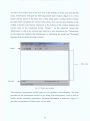
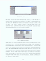
and
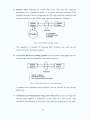
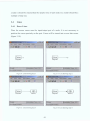
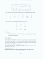
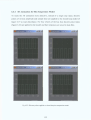
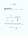
a) Remote S&A: Through an HTML data entry form the user specifies
parameters for a simulation model. A Common Gateway Interface (CGI)
transfers the data to server; an appropriate CGI script starts the simulation and
prints the results in a new HTML page when the simulation is finished.
Fig 2.4: Remote S&A and data transfer
This approach is suitable for existing S&A software, but user has no
interaction with a running simulation.
b) Local S&A Based on Loading Applets: the user loads a Java applet into the
web browser, runs the simulation on the client machine.
1. Call for an applet
2. Download the applet
3. Run the applet and show results
Fig 2.5: Client-Site simulation with loaded applets
It supports user interaction and animation, but not suitable for the existing
S&A tools.
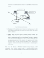
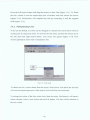
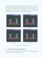
c) Animation and Manipulation using a Java Data Server: the user begins by
loading some applets; a connection is then built to a Java server. The
simulation runs remotely on this server, the results are transferred to the client
26
browser, and visualized locally. The user can interact with the model by using
buttons on the HTML page.
Fig 2.6: Remote simulation and local visualization
Finally the paper introduces Skopeo, a Java-based, platform-independent 2DAnimation system.
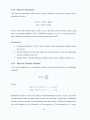
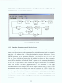
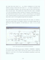
Yiicessan, et al [30] introduces a Parallel Discrete Event Simulation (PDES) support
system to distribute simulation experiments over the Internet. There are several
approaches to exploiting parallelism in discrete event simulation; unfortunately each
of those has its own drawbacks. For example, a) in Dedicated Execution approach,
where dedicated functional units execute specific sequential simulation functions, the
speed tends to be limited as the management o f the future events list becomes the
bottleneck, b) in Hierarchical Decomposition, where a model is decomposed in a
hierarchical fashion such that an event consisting o f several sub-events to be
processed concurrently, is largely model dependent, c) in Parallel Replication, where
several replications o f a sequential simulation are executed independently on different
processor, each processor must contain enough memory to hold the entire model. The
paper describes a prototype o f a software architecture that would support PDES. The
main objective o f the proposed system is to plan parallel simulation experiments and
dynamically manages their execution. Via the Internet the system has access to a large
number o f sites (a PC or Workstation), from where it can dynamically selects one to
execute part (parallel replication) o f an experiment. The system uses OCBA [31] to
implement the experiment planner. The system has also data collection and analysis
capabilities to collect and analyse output data from each individual processor. Finally,
27
the system contains a reporting mechanism, which compiles and presents the result in
a multimedia format, consisting of tabular and graphical summaries.
Veith, et al [32] presents Netsim, a discrete event simulation package based on the
event graph approach. Netsim provides a maximum amount o f user interaction with
the simulation model. A programming interface provides a blank template with text
fields for the various parameters of a simulation model, such as event name and state
variables. A second interface allows user interaction with running the simulation
model. This interface not only provides start, pause and stop capabilities and data
output, but also an animation o f the model. The object-oriented structure offered by
Java and maintained in Netsim allows easy expansion of the package as well as
compatibility with other Java-based tools.
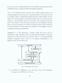
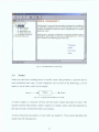
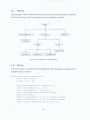
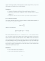
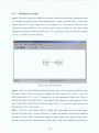
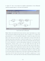
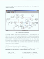
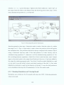
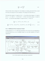
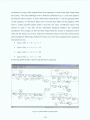
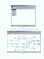
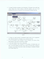
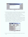
Elmaghraby, et al [33] demonstrate a software model that can be used for
transforming a legacy simulation system into Web-accessible application. The paper
describes the initial results from the conversion effort on an existing distributed
simulation visualization system. There are two potential methodologies to run
application from the World Wide Web.
Fig 2.7: Web-enabling software model
a) to develop the application to be web aware using Web development
techniques such as: HTML, Java, CGI etc.
28
b) to transform an already existing application, which was not designed for the
web, into a Web-accessible application.
But there are a number of problems to convert an existing application to be web
accessible, such as limited environment, security risks, concurrency etc. To answer all
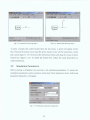
this problems a Web-enabling software model has been introduced. The proposed
layered model (figure 2.7) has several layers to link an existing application to a web
browser. The Web browser layer is the interface layer where users can interact with
the application from the Web. Authentication layer authenticates the user and
validates the login name and password. The environment set-up layer will control
concurrency, create run profile and talk to the listening daemons layer, which is the
heart of the model. Listening Daemons layer receives user request and the start-up
settings then launches the Distributed Simulation.
Salisbury, et al [34] discusse a browser-based simulation visualizer that has the ability
to display simulated entities to any number o f distributed sites. Legacy visualizers
have a number o f drawbacks, such as, the tool must be present at the inception o f the
simulation, no matter the observer is only interested to observe a relatively small time
slice. Most existing visualization tools are dependent on the machine for which the
application was written. The paper introduces a tool Jview-lite to solve these
problems. Jview-lite is the successor o f a modular programme Jview, which supports
the simulation community’s diverse set of visualization requirements. Jview relies on
Sun’s Java 3D architecture to render an image, and the use o f Java Beans enables it to
display objects from any data source. Jview-lite utilizes the same display technology
but relies on the Web for distribution. The client server architecture, proposed for
Jview-lite, has two principal software components: the Simulation Monitor and the
Simulation Viewer. The Jview-lite simulation viewer is an applet executing within the
client’s web browser. On receiving a request from a client’s browser, the web server
will send the required page and the embedded viewer applet. The browser then
initializes the viewer applet, effectively making the browser a 3D-simulation viewer.
The viewer, in turn, makes contact with the simulation monitor that is residing on the
same machine as the web server. The monitor passes object information to the client.
The simulation viewer can then render the simulation based on this information.
29
Schmid [35 - 40] presents a remote laboratory approach using virtual reality on the
Web, where an audio-visual interface together with a collaboration tool gives the
feeling of being in the laboratory. Most existing virtual labs offered across the Web
include several fully interactive experiments completely written as Java applets, but
can’t claim to be an equivalent substitute of the real experiment. To solve the
problems of this “close-to-reality” environment and to take the full advantage of a
remote virtual laboratory, preference is given to an architecture where all
computational work is performed locally using some existing computational machines
like MATLAB/SIMULINK/MAPLE and the output is linked to the objects o f VR
scene. One main task to accomplish this is to tie together the computational machines
of MATLAB/SIMULINK/MAPLE with Web components to a hypertext-based
system, which runs on the Web browser. The proposed client/server architecture uses
the following plug-ins for this purpose: MATLAB plug-in integrates MATLAB
operation into the Web browser, the Graphics plug-in extends the MATLAB plug-in
to view MATLAB or Metafile graphics, the DDE server plug-in, together with the
VRML plug-in, is for viewing and acting with VR scenes. The paper concludes with
some examples to demonstrate the architecture.
Guru, et al [41] introduces a web-based interface for storing and executing simulation
models, developed using SIMAN simulation language, over the Internet. This toolkit
consists of a World Wide Web interface to SIMAN and a web-accessible database for
storing the models. To use the system, a user simply needs access to the Internet and
an account on the web server. It allows user to develop, execute and test the
functionality o f a model through the use o f the SIMAN debugger/run controller. The
proposed system involves three servers.
a) Application server: An Internet user accessing the Web address for the site is
directed to this server. The software residing here performs the functions of
authenticating the user and providing access to user’s models in the database.
It gives the user the capability to edit, add or delete models in his/her account.
When user wants to compile, execute or debug a model, this server creates an
appropriate HTML document (dynamically-generated), which contains the
30
instruction o f the desired operation and pass it to the SIMAN server on user’s
request.
X
X
Firewall
Fig 2.8: Hardware and software layout
b) Oracle server: The application server interacts with the Oracle server in order
to provide accessibility to the user’s models. The models and the user data are
stored in a database.
c) SIMAN server: This server holds the SIMAN simulation software. The
SIMAN simulation software performs the requested operation and returns the
results to the user in the form o f an HTML document. This done by piping the
output o f the appropriate SIMAN process that are invoked with the CGI script
as a dynamically-generated HTML document. The arguments to the SIMAN
process are ASCII text files containing the SIMAN model. These files are
temporarily created by CGI scripts with the data posted to them through the
HTML forms.
Marr, et al [42] discusses a Web-based simulation manager program, called
SimManager, which executes simulation study in a parallel-replications mode,
utilizing a set o f slave processors available to it. Slave (engine) processors need not be
31
co-located. They can belong either to an intranet, to the Internet, or to a combination
thereof. An engine is simply known to SimManager by its IP address. SimManager
also knows the performance characteristics o f each engine. SimManager would serve
as the interface between a customer seeking assistance in simulation modelling and
the simulation system. When the customer accesses the web page, he would click on
the Catalog of Simulation models and view a description of any models that appear to
meet his specific needs. SimManager receives this request for work and places it in
the job queue. After determining what engines are available for work it assigns this
workload to the engine processor. It also receives back a file containing the statistical
results derived from the engine’s efforts, and organizes these results into a form that
meets the needs o f the customer. Once all the jobs associated with the customer
request are complete, an email message is sent telling him that the results are ready
for pick up.
Rao, et al [43] present WESE: A Web Based Environment for Systems Engineering.
The design and development of modem systems is complicated by their size and
complexity. Furthermore, many o f today’s complex systems are built using
subsystems and components available from third party manufacturers. Using WESE, a
developer can analyse different design alternatives involving components from
various researchers and manufacturers. The environment provides a flexible
framework to develop formal specifications and verify the designs using mechanized
theorem proving. WESE also provides the techniques to generate different
specifications documents such as cost of the system.
The primary input to WESE is a System Specification Language (SSL) description of
the system. The input SSL source is parsed into an intermediate form (SSL-IF) using
a parser. SSL-IF forms the input to other modules of WESE SLL-IF is used to
construct simulations, generate specifications, and documentation from the distributed
factories. The factories play a pivotal role in providing a uniform interface to generate
the various components specified in the SSL specifications. The various subsystems
o f WESE provide necessary support to achieve the different functionalities of
environment. The user may employ a hypertext markup language (HTML) or a text
based interface to interact with the environment.
32
The rapid advances in Web technology, most notably Java, enable to execute highly
interactive and dynamic simulations/animations on the Web. Java [44] is a portable
language because it is compiled into an architecture neutral, byte code format. Hence,
a Java application can run on any system, providing that system implements the Java
Virtual Machine (JVM). It is this portability, which makes Java so attractive to
Internet developers because it allows compiled Java code to be sited on one computer,
but downloaded, interpreted and executed on another computer; which isn’t
necessarily running on the same platform without the need to recompile the software.
This is of significant difference to more traditional simulation languages such as C++,
where exporting simulation code requires recompilation and installation on each
different machine. Although Java is a small core language it does support extensive
class libraries.
As a result the JVM need only be able to handle the core o f the
language whilst applications can be developed using the class libraries. These class
libraries can be further refined and extended to develop application specific packages
(e.g. simulation). All versions o f Java come with a set of in-built class libraries which
include facilities for developing graphical user interfaces (e.g. the java.awt and
javax.swing.awt packages) [45], network application support (java.net package), a
number of utility functions (java.util package), remote method invocation (java.rmi
package) and 3D animation facility (Java 3D API) [46].
The facilities provided by the Java programming language to support Web technology
is the power behind Web-based simulation. Java benefits from being simple, secure,
object-oriented, multi-threaded and architecture neutral. More and more researchers
develop their simulation packages based on Java. But most o f this research is only
devoted to discrete event simulation. SimDynamic is an attempt to introduce dynamic
system simulation on the Web and provides a positive, unique contribution to Web
based simulation.
33
Chapter Three
3
Overview of SimDynamic
3.1
W hat is SimDynamic
Sim D ynam ic is a jav a based sim ulation package for m odelling, sim ulating and
analysing dynam ic system s on the Web. A model o f m oderate com plexity can be
constructed with m inim um o f effort and w ithout w riting any code. It supports linear
and non-linear system s, m odelled in continuous time, sam pled time or a hybrid o f the
two. Finally the package will provide both numerical, graphical results and also 3D
animation.
Sim D ynam ic is actually a collection o f several functional nodes, where each node
carries out a specific function such as integration, generation o f sine wave,
m ultiplication etc. These nodes serve as the basic building blocks o f a model. These
are classified into following eight node sets
•
C ontinuous
•
N onlinear
•
Discrete
•
M iscellaneous
•
Tables
•
Sinks
•
M ath & Logic
•
Source
The package has been designed with an aim to achieve as much modelling ease as
possible and to provide m axim um user flexibility in model execution. For m odelling
the package provides a graphical user interface (GUI) for building m odels as block
diagram s, using simple m ouse operations. A block diagram is a pictorial model o f a
dynam ic system. It consists o f a set o f nodes, interconnected by lines. Each node
produces an output either continuously (a continuous node) or at specific points in
tim e (a discrete node). The lines represent connections o f node inputs to node outputs.
A block diagram can contain any num ber o f instances o f any type o f node needed to
model a system. This interface will enable the user to draw a block diagram ju st as to
draw with pencil and paper.
34
Section 3.2 contains a b rief description o f the GUI, section 3.3 focuses on the
m anipulation o f nodes provided by Sim D ynam ic, section 3.4 deals with lines, section
3.5 introduces the sim ulation param eters, section 3.6 gives a b rief description o f how
to build a model using the package and section 3.7 presents how to make 3D
animation.
3.2
G raphical U ser Interface (G UI)
W hen Sim D ynam ic is started it opens the node set w indow (figure 3.1). This window
is divided into three sections. First section contains the nam e o f the currently selected
node set, second section shows all the eight node sets provided by Sim D ynam ic, and
the final section displays the nodes in the currently selected node set.
¿11 Dynamic Simulation System on The Web
File
New Icon
Edit View
Help
D U
Name of the
currently
selected node
set
SimDynamic : Math & Logic Node Set
+
£ l
Node Sets
Continuous
Discrete
Tables
\
Non Linear
Sinks
IA |
Absolute
A&B
Bitwise Logic
Combinatorial
Logic
Gain
=D-
a + ib
Magnitude Angle
to Complex
Ja va Applet Window
Fig 3.1: Node set window
35
X
Math & Logic
/
Miscellaneous
Logic O perator
---
Sources
A. B
Dot Product
powlO
Math Function 1
Nodes in the
currently
selected set
To start a new m odel click on the new icon in the toolbar, or select new from the file
menu. Sim D ynam ic will open the following model sheet w indow (figure 3.2). A new
m odel will be draw n in the draw area o f this blank sheet. Toolbar o f this w indow
provides short cut buttons for various m enu items. User can use these buttons on the
toolbar at his/her convenience. Status-bar at the bottom o f the window displays the
current state o f the sim ulation model. “Ready “ on the status-bar m eans that
Sim D ynam ic is idle at the m om ent and ready for a new sim ulation run. “Initialising”
on the status-bar indicates that Sim D ynam ic is initialising the model and “R unning”
indicates that the model is being executed.
SI| SimDynamic : Untitled*
File
Toolbar
Edit View
Q B B s
Simulation
Help
«
Draw Area
Statusbar
—^
Ready
[simulation Time : 0.0
Ja va Applet Window
Fig 3.2: Model sheet window
The interface incorporates on-line help for user guidance and assistance. The help
provides all the inform ation needed to get along with Sim D ynam ic, such as how to
build a model, sim ulation param eters, functional description o f nodes etc. Figure 3.3
provides a screenshot o f Sim D ynam ic on-line help.
36
-|nl x
'D SimDynamic Help
«
What is
■ lO K I
23 SimDynamic Help
♦ Introduction
SimDynamic?
-
SimDynamic is a java based simulation package for modelling, s
jE B ® æ
of moderate complexity can be constructed with minimum of effo
systems, modelled in continuous time, sampled time or a hybrid
graphical result.
• Build a Model
f • Run a Model
• Manipulate Lines
• Manipulate Nodes
♦ Simulation Parameters
g
Node References
SimDynamic is actually a collection of several functional nodes,»
integration, generation of sine wave, multiplication etc. These nc
are classified into following eight node sets
* Continuous
* Tables
* Hon Linear
* Sinks
J
<L
IJava Applet Window
Fig. 3.3: SimDynamic on-line help
3.3
N odes
Nodes are the basic building block o f model. Each node perform s a specific task at
each sim ulation tim e step. A node com prises one or more o f the following: a set o f
inputs, a set o f states, and a set o f outputs.
States
Input(s)
Output
Fig 3.4: Logical representation of a node
A node’s output is a function o f time and the n o d e’s inputs and states (if any). The
specific function that relates a node’s output to its inputs, states, and time depends on
the type o f node o f w hich the node is an instance.
To have functional description o f each node see chapter 5. This section describes the
nodes from GUI perspective.
37
3.3.1
A d d in g a N o d e
To add a node in the model sheet, click on the node in the node set window. The
mouse cursor will be turned into a hand cursor indicating that the node has been
selected. N ow click on the draw area o f model sheet window. Sim D ynam ic will add
the selected node in the model sheet. Each node will have one or more input/output
port.
3.3.2
M a n ip u la tin g N o d es
To move a node w ithin the model, place the m ouse cursor on it and press the left
m ouse button. M ouse cursor will turn into a crossed cursor. Now drag the m ouse and
the node will be m oving with the m ouse movement. If any line is connected to the
node it will be adjusted automatically.
A node can be deleted, rotated or renam ed by using node menu. To activate the node
menu, position the m ouse cursor on the node and click the right m ouse button. The
node menu will appear like figure 3.5. N ow choose appropriate menu item to
m anipulate the node.
-In l x|
JD SimDynamic : Untitled*
File
Edit View
Simulation
Help
H
i# 5
1
1
a
Derivi
l>
D elete
Rename
Rotate
Help
Ready
imulationTime : 0.0
Window
Fig 3.5: Node menu
To delete the node select delete from the menu, the node will be deleted and the
connected lines (if any) to the node will be adjusted.
38
To renam e the node choose rename from the menu, Sim D ynam ic will open a dilaog
box, enter the new nam e o f the node and click ok on the dialog box. The new nam e
will appear at the bottom o f the node.
To rotate the node choose rotate from the menu, the node will be rotated by 180
degree.
3.3.3
S ig n a ls an d D a ta T y p es
Signals are the stream s o f values that appear at the outputs o f a node when a model is
simulated. It is useful to think o f signals as travelling along the lines that connect the
nodes in a block diagram. But it should be kept in m ind that the lines in a model
represent logical, not physical, connections am ong nodes.
The term data type refers to the w ay in w hich a com puter represents num bers in
memory. Different machines (with different architectures) allocate different am ount
o f storage and uses special internal codes to keep track o f the different types o f data it
processes. On the other hand, a data type in a program m ing language is a set o f data
with values having predefined characteristics. Exam ples o f data types are: integer,
floating point, character, string, and pointer. It is a collection o f values and operations.
Operations do things to values and produce values as a result.
Sim D ynam ic supports two types o f signal i) N um erical and ii) Boolean. The prim itive
data type used by Sim D ynam ic for num erical values is Java double, which is a 32 bit
signed number. So it ranges from 1.7e'308 to 1.7e308. Sim D ynam ic supports both real
and com plex num bers, and for logical operations it internally converts the double
value to integer.
Boolean value is used for some logical operations. There are some nodes that support
both types o f data. It is up to the user to decide w hether Boolean value or num erical
value is to be used.
3 .3.4
N o d e P a ra m e ters
N odes are added to the models with their default param eters. Each node has its own
param eter dialog box to set param eters. To access a node's param eter double click on
39
it, param eter dialog box o f the corresponding node will be opened. N ow the user can
change param eter values. After changing the param eter values click the ok button on
the dialog box. A click on the cancel button will ignore any change in the param eters
and will retain the previous param eter values. Param eter Dialog Box for Discrete
State Space node is shown here for example.
Parameters for Discrete
State-Space
X]
-Parameters
A matrix
F
B matrix
F
C matrix
F
D matrix
F
Initial Condition
p
Sample Time
F
Cancel
Ok
J a v a Applet Window
Fig 3.6: Parameter dialog box for Discrete State Space
M ost nodes accept vector (ID array) or matrix (2D array) param eter/input. There are
some nodes that accept only single number. V ectors m ay be o f two types i) row
vectors (2D array contains only one row), ii) colum n vector (2D array contains only a
single column). To enter a row vector as param eter write the num bers separated by
spaces. Follow ing dialog box shows, how to enter the row vector 2 3 4 as Gain
param eter,
Parameters for Gain
*I
Parameters
Gain Value
|2 3 4
Ok
Cancel
J a v a Applet Window
Fig 3.7: Row vector as parameter
40
To enter colum n vector as param eter write the num bers separated by com mas. Figure
3.8 shows how to input a colum n vector as gain param eter
Parameters for Gain
x]
Parameters
Gain Value
Cancel
Ok
Ja va Applet Window
Fig 3.8 : Column vector as parameter
To enter a m atrix as param eter enter the rows one by one separated by com mas.
Follow ing dialog box shows, how to enter the following m atrix as Gain param eter
I Parameters for Gain
* ]|
r a r a m e ie r s
G ain Value
|2 3 4.5 6 7.1 3 5
Ok
C a n ce l
Ja va Applet Window
Fig 3.9 : Matrix parameter
M ost o f the nodes support auto expansion o f inputs/param eters w herever applicable.
For exam ple 2 3 4 has been entered as gain param eter and the node receives 5 as
input. Then Gain node will consider the input as 5 5 5 and output will be 10 15 20.
For m atrix param eter the node will try to expand the input to a matrix o f same
dim ension as the param eter. For exam ple above m atrix has been entered as gain
param eter and the node receives 7 as input. Then gain node will expand the input to
the following m atrix,
41
I
l
l
1
1
1
1
1
1
And the corresponding output from the node will be the following m atrix,
14
21
28
35
42
49
7
21
35
W hen using m atrix input or param eter, it should be made sure that all the rows o f the
m atrix m ust have same num ber o f columns.
3.3 .5
D irec t F ee d th ro u g h
There are some nodes whose current outputs depend on their current inputs. These
nodes are defined as direct feedthrough nodes. All other nodes are called non-direct
feedthrough nodes. Exam ples o f direct feedthrough nodes are Sum, Gain etc.
Exam ples o f non-direct feedthrough nodes are Integrator, M em ory etc. W hen using
direct feedthrough nodes it should be made sure that the model does not contain any
algebraic loop. An algebraic loop generally occurs w hen an input port w ith direct
feedthrough is driven by the output o f the same node, either directly, or by a feedback
path through other nodes with direct feedthrough.
3 .3 .6
S a m p le T im e
The Sample tim e param eter sets the time interval at which node’s states (output) are
updated. There are some nodes that have continuous (all the nodes in continuous node
set and some other) sample time, some nodes have discrete sample time (all the nodes
in discrete node set and some other). There are some nodes, which derive its sam ple
time from its driving node (the node from which it receives its input), these nodes are
said to have inherited sample time. W hen a node has inherited sample tim e and it
receives its input from more than one node, then it sets its sample time to the sam ple
tim e o f the driving node that has the fastest sample time. W hen setting sample tim e o f
42
a node it should be ensured that the sample tim e o f each node in a model should be a
multiple o f step size.
3.4
Lines
3.4.1
D ra w L in es
Place the m ouse cursor near the input/output port o f a node. It is not necessary to
position the cursor precisely on the port. C ursor will be turned into a cross hair cursor
(figure 3.10).
-inlxi
I'D S im D y n a m ic : U n t i t l e d 4“
File
Edit View
Simulation
IB1SE1B
j
hh
a
2D S im D y n a m ic : U n title d *
Help
File
a
1
Edit View
O Ö H #
jsimulation Time : 0.0
Ready
*-b
|simulation Time : 0.0
Ja v a Applet Window
Fig 3.10: Line drawing step 1
Fig 3.11 : Line drawing step 2
D S im D y n a m ic : U n title d
File Edit View Simulation
Jnjxj
_'D S im D y n a m ic : U n title d *
Edit View
S3
Integrator
Ja v a Applet Window
File
Help
H SU
Jrm
>+
Integrator
Ready
Simulation
Simulation
Help
G lgSH
Help
HH
m dt
Integrator
Ready
Memory
Integrator
[Rei
1Ready
imulation Time : 0.0
Ja v a Applet Window
Memory
imulation Time : 0.0
| J a v a Applet Window
Fig 3.12: Line drawing step 3
Fig 3.13: Line drawing step 4
43
Press the left m ouse button and drag the m ouse to draw line (figure 3.11). To finish
the line, extend it near the output/input port o f another node and release the mouse
(figure 3.12). Sim D ynam ic will com plete the line by connecting it with the targeted
node (figure 3.13).
3.4.2
M a n ip u la tin g L in es
A line can be deleted, its colour can be changed or a branch line can be draw n from an
existing line by using line menu. To activate the line menu, position the m ouse tip on
the line and click right m ouse button. Line menu will appear (figure 3.14). Now
choose appropriate menu item to m anipulate line.
SD SimDynamic : Untitled*
File
Edit View
Simulation
Help
>
Memory
Color
Branch
Help
| Ready
m e: 0.0
jjava Applet Window
Fig 3.14: Line menu
To delete the line, choose delete from the menu. Sim D ynam ic will delete the line and
will reset the input/output port o f the node to w hich the line was connected.
To change the colour o f the line, select color from the menu. Sim D ynam ic will open a
colour chooser, select a new colour and click ok button. The line will be redraw n in
the new colour.
44
File
□i &
Edit View
a m
Simulation
► •
Help
?
f
Integrator
Ready
|simulation Time : 0.0
Ja v a Applet Window
Fig 3.15: Branch line drawing step 1
Fig 3.16: Branch line drawing step 2
To draw a branch line, select branch from the line menu. A point will appear on the
line. Position the mouse cursor near the point, m ouse cursor will be turned into a cross
hair cursor (figure 3.15). N ow press the left m ouse button and drag the m ouse to draw
branch line (figure 3.16). To finish the branch line, follow the same procedures as
with normal lines.
3.5
Sim ulation P aram eters
Before starting a sim ulation run user has to set simulation parameters. To access the
sim ulation param eters select param eter menu item from Simulation menu. Following
param eter dialog box will appear.
D Simulation Parameters
on i miauui i i line
Start Time|oo
Stop Tir nejlO.O
nueyi diui
Select Integrator
|None
Step Length
¡0.2
Cancel
i
Java Applet Window
Fig 3.17: Simulation parameters dialog box
45
3.5.1
S im u la tio n tim e
Sim ulation time specifies how long the sim ulation will continue. This time is
m easured in seconds. And o f course it is in pseudo time. Starting tim e need not be
always 0. Sim ulation may start from any starting time. The only requirem ent is that
stop time must be greater than the start time.
It should be noted that, sim ulation time and physical time are not the same. For
exam ple, running a sim ulation for 10 seconds will usually not take 10 seconds. The
am ount o f tim e it takes to run a sim ulation depends on m any factors, including the
m odel’s com plexity, the sim ulation step sizes, and the com puter’s clock speed,
available m em ory etc.
3.5.2
In te g ra to r
The dynam ic models are generally described by differential equations. The solutions
o f these equations display the operations o f the system and this is the fundam ental
property o f dynam ic models. This software provides a num ber o f integrators to solve
ordinary differential equations (ODE). Because o f the diversity o f dynam ic system
behavior, some integrators m ay be m ore efficient than others at solving a particular
problem. Here is a b rief description o f each solver that has been im plem ented. Greater
details about integrators can be found in chapter 4.
•
R K D P : It is based on an explicit Runge-K utta formula, the D orm and-Prince
pair.
•
R K _0 4 : It is based on fourth order explicit Runge-K utta formula.
•
R K B S : It uses an explicit Runge-K utta pair o f Bogacki and Shampine. It m ay
be more efficient than RK DP in the presence o f mild stiffnes.
•
R K H E : It uses H eun’s m ethod which also known as m odified Euler formula.
•
R K E U : It uses simple E uler’s m ethod for integration.
3.5 .3
S tep L en g th
Sim D ynam ic starts at the starting tim e and advances its clock by adding step length to
the current clock time until it reaches the stop time. At every time step it calculates
the output o f each node in the model. Default tim e step is 0.2. So for a start time 0 and
46
stop tim e 10.0, outputs will be calculated at 0, 0.2, 0 .4 ............ 10.0. Sm aller tim e steps
m ay ensure m ore accurate results but at the same time it m ay increase sim ulation run
tim e depending on the model com plexity and the integrator used.
Step length and sample time o f the nodes in a model m ust be com patible. W hen
setting step length or sample time o f nodes, it should be made sure that sam ple time o f
all the nodes in a model must be an integer m ultiple o f the step length.
3.6
Run a M odel and View O utput
Sim ulating a dynam ic system with this package is a two-step process. First, the user
has to create a model o f the system to be simulated. The model graphically depicts the
tim e-dependent mathem atical relationships am ong the inputs, states and outputs o f the
system. A fter the model creation user has to choose an integration m ethod and then
can use Sim Dynam ic to simulate the behaviour o f the system for a specified period o f
time.
To start a sim ulation run choose run from the sim ulation m enu or click on the run
button from the toolbar. First Sim D yanm ic will initialise the model and then it will
execute the model. If the model does contain error, sim ulation will be halted with
appropriate error message.
To view result o f a sim ulation run, use the nodes (except term inator node) from Sink
node set. To view numerical result use D isplay node, for graphical results Time vs
input or X vs Y Graph nodes can be used. To save sim ulation results in a text file use
To file node. W hen sim ulation run is finished sim ply double click on any o f the sink
nodes to view results. To D at File node from the sink node set can be used to save
sim ulation results in a data file for later use by Sim D ynam ic.
3.7
3D A nim ation
To start the 3D model editor, choose 3D animation from the sim ulation menu.
Sim D ynam ic will open the following 3D model editor.
47
E>S im D y n a m ic : 3D M od el Editor
^ jD jx jl
Box
Edit
Cone
Remove
Cylinder
Save
Sphere
Load
Param
.
Run
Fig 3.18: 3D model editor window
This editor provides some basic 3D shapes (Box, cone etc.) on the left side. It is
assum ed that the 3D model will be rendered in a 3D space. At each sim ulation time
step objects o f a 3D model will m ove to a new position in the space. User has to add
3D shapes to the space to construct a model. To add any shape, click on the
appropriate button. Each button click will open a dialog box for the selected shape.
Here param eter dialog box for a box is shown for exam ple,
|A d d a b o x t o m o d e l
Width
|o i
Center x jo
Height l°i
Center y| o
Red
Green
fT ”
File name forx
h
|None
File namefory
|lMone
File nameforz
|fMone|
Add
■
Depth
JD
|o.1
Center z|o
Blue
¡0
Cancel
J
_
Fig 3.19: Dialog box for 3D box
On the dialog box user has to define the initial position (center X, Center Y, Center
Z), colour (in term o f RGB value) and dim ension o f the shape. All the dim ensions in
the 3D model editor are m easured in meter. M ore im portantly, to anim ate any 3D
object at least one data (sim ulation result from SimDynamic) file should be associated
with it. 3D anim ator will read current position o f the object from the associated data
file(s) and render the 3D animation. Param eter button enables the user to set some 3D
param eters. User can set the origin o f the 3D space and can also set the time delay
during 3D rendering. Save button can be used to save a 3D model. U sing the load an
existing 3D model can be opened. To start 3D anim ation, click the run button and a
new 3D w indow will be opened.
48
Chapter Four
4
T h e D e sig n o f Sim D ynam ic
SimDynamic, is a collection o f Java classes (objects) which provides basic utilities for
constructing simulation models for dynamic systems. In the current implementation,
simulation, random number generation, and analysis o f simulation result (both
numerical and graphical) are built into the library. In the following sections, the
design of the Simdynamic package will be presented in great detail.
SimDynamic is intended to make model creation an easy task. It is also intended that
the model user would be able to understand the model as well as use the simulation
easily. This is achieved through providing a user-friendly modelling interface and an
easy to view (graphical/numerical) results mechanism. It is believed that SimDynamic
is an easy to use package and that even a fairly complex simulation model can be
constructed without writing any additional code.
The software consists of three packages, each package containing a set o f related
classes that work together to provide functionality in a key area to support a
simulation process. The package hierarchy of this software is shown in figure 4.1.
Fig 4.1 : SimDynamic package hierarchy
A discussion o f each of these packages is presented in this chapter in greater detail. In
the class hierarchy diagrams in this chapter foundation classes (Java built-in classes)
are represented by dashed rectangle and software classes are shown by regular
rectangles. The signatures for the public methods o f major classes for each package
will be given. For brevity, all the classes of each package, and all the methods of
classes, are not discussed here. Complete source code of SimDynamic is provided in
appendix E.
49
4.1
UlPack
This package contains all the necessary classes to provide the graphical user interface
(GUI) o f the software. The class hierarchy o f this package is as follows
Fig 4.2 : Class hierarchy in UlPack package
4.1.1
M yL ine
The MyLine class is responsible for handling all the line drawings in a model, and its
definition looks as follows
public class MyLine extends Object{
public Vector points;
private int lx, ly;
public MyLine(Container c, Simulator s);
public void drawL(Point p, int d);
public void drawC(int w, Color clr);
public void setArrowPoints(boolean rotated);
public void drawA();
public void adjustA(int tx, int ty, boolean rotated);
public void adjustR(int tx, int ty, boolean rotated);
public boolean
checkpoint(Point p, Point pt);
}
50
This implementation of MyLine allows only vertical and horizontal lines. A complete
line may contain indefinite number of vertical and horizontal segments. MyLine
stores end points of every segment in the Vector points, lx and ly stores the last
drawing point o f the line. Constructor needs a Container on which the line will be
drawn and a Simulator which will store the line.
Method drawL draws a line segment from (lx, ly) to the current point p. This method
also determines the direction (vertical or horizontal) of the line.
The drawC method draws a circle at the last point of an incomplete line.
The setArrowPoints method calculates the co-ordinates of an arrow for a completed
line.
The drawA method draws an arrow at the last point of a completed line.
Method adjustA and adjustR are used to adjust a line connected to a node, when the
user moves the node.
4.1.2
H elpFram e
HelpFrame provides the framework for displaying SimDynamic online help.
HelpFrame extends DefaultHelpBroker{
public HelpFrame(HelpSet hs);
}
HelpFrame simply extends jav a’s DefaultHelpBroker, where the HelpBroker is the
default presentation o f a HelpSet. And a HelpSet is a collection of help information
consisting o f a HelpSet file, table of contents (TOC), index, topic files, and Map file.
The constructor also customizes the default presentation by enabling and disabling
some buttons.
4.1.3
D raw A rea
Class DrawArea provides the free area on the model sheet window, where user can
draw a model. Its signature is as follows,
class DrawArea extends JPanel implements ActionListener{
public DrawArea(Simulator smltr);
public void painComponent(Graphics g);
public void actionPerformed(ActionEvent ae);
public Nodeicon createNode();
51
}
Constructor DrawArea initialises the drawing area and it also implements the
ActionListener interface to perform the menu actions for a line. This class also
includes two inner classes to capture all the user mouse operations.
The paintComponent method repaints the draw area when ever it is needed.
The actionPerformed method handles all menu actions for the line menu.
The createNode method creates a new node, when ever user clicks on the draw area
after selecting a node from the node set browser, and returns the node.
4.1.4
B lankSheet
Class BlankSheet holds the DrawArea and provides the framework for simulation
model sheet window. It looks like as follows,
public class BlankSheet extends JFrame implements ActionListener{
public BlankSheet();
public void processComponent(ComponentEvent ce);
public void actionPerformed(ActionEvent ae);
Constructor BlankSheet performs all the necessary steps to set the UI. It instantiates a
new DrawArea and add it to the frame, also instantiates menu and menu items,
toolbar, and status bar.
The processComponent method is used to store the current size and location o f the
frame, whenever it is resized or moved by the user.
The actionPerformed method handles all the menu actions and toolbar icon actions.
Other than these methods, this class has two important private methods saveFile() and
openFile(). These methods are used to save a model or to open an existing model.
4.1.5
M ainFram e
MainFrame class is responsible for the node set browser window, which is the
starting window o f SimDynamic.
public class MainFrame extends JFrame implements ActionListener{
public MainFrame();
52
public void actionPerformed(ActionEvent ae) ;
Constructor MainFrame, instantiates all the components necessary for the user
interface (UI).
The actionPerformed method is responsible for all menu actions and toolbar icon
actions. This method also creates a new BlankSheet whenever user clicks the new
menu item.
4.1.6
P aram F ram e
Class ParamFrame enables the user to set simulation parameters. Its signature is as
follows,
public class ParamFrame extends JFrame implements ActionListener{
public ParamFrame(Simulator smltr);
public void initParams();
public void actionPerformed(ActionEvent ae) ;
Constructor ParamFrame instantiate all the components needed for the input such as
TextField, ComboBox etc.
The initParams method assign the current values o f different simulation parameters to
the respective input fields before displaying the frame.
The actionPerform method is invoked when user clicks any o f the buttons (ok/cancel)
in the frame. This method parses the input entered by user and checks legitimacy of
input. Invalid input will be reported by appropriate error message.
4.1.7
O ther C lasses in the Package
UlPack also contains following classes. All o f these classes (except CNST class)
extends JFrame.
CNST - this class holds some constant values that are used in various places of the
software. All members of this class have been declared static. So they are directly
accessible by using the class name only.
53
ColorFrame - Color Frame provides a colour chooser, using that user can change the
colour o f a line.
ErrorFrame - SimDynamic uses ErrorFrame to display the appropriate error
message, whenever it encounters some error during the runtime o f a simulation.
InfoFrame - this class displays the information about SimDynamic.
DispFrame - DispFrame provides the framework to display numerical results o f a
simulation. The class SnkDspl from NodePack package supplies the numerical results
to this class after a simulation run is completed.
TvsXFrame - this class is responsible for graphical output o f a simulation. It plots the
graph o f a simulation result with respect to time. The class SnkTvsinp from NodePack
package provides necessary data to this class.
XvsYFrame - works in the same way as TvsXFrame, but it derives its data from the
class SnkXYGrph of NodePack package.
4.2
NodePack
NodePack is the core o f this software and provides all the functional nodes. This
package also contains the main simulation engine (the Simulator class) and some
other important classes.
Fig 4.3 : Class hierarchy in NodePack package
54
4.2.1 Basic
Basic class can be considered as the utility class for SimDynamic. This class contains
various utility methods to ease the task o f other classes.
Basic extends Object{
public static boolean equalTo(double dl, double d2);
public static boolean grTeqt(double dl, double d2);
public static boolean IsTeqt(double dl, double d2);
public static boolean lessTn(double dl, double d2);
public static boolean greatTn(double dl, double d2);
public static boolean checkRegion(int x, int y, int cx,
int cy,
int r);
public static void VecToArray(double[][] R,double[][] C,
Vector V);
public static void VecToArray(double[][] M,Vector V);
public static void VecToArray(double[] R,Vector V) ;
public static byte setOpDataType(Vector opMat);
public static void dblVect2cmplx(Vector cmplxV, Vector dblV);
public static void assignVect(Vector VI, Vector V2);
public static void assignMat(Vector Matl, Vector Mat2);
public static boolean isNegative(Vector Mat);
public static boolean hasGreater(Vector Matl, Vector Mat2);
public static Vector matMultByVec(Vector Matl, Vector Mat2);
public static void getDim(Vector Mat, MyDim d);
public static boolean between_include_lower(double n,
double h, double 1);
public static boolean between_include_higher(double n,
double h, double 1);
public static boolean between_include_both(double n,
double h, double 1);
public static Double elementAt(Vector Mat, int row, int col);
public static Boolean elementAt(Vector Mat, int row,
int col, byte b);
public static boolean elementAt(Vector Mat, int row,
int col, Complex cmplx);
public static void initMat(Vector Mat, double dbl);
public static void initMat(Vector Mat, double rel, double img);
public
static
boolean
canBeResolved(MyDim
diml,
MyDim
dim2,
boolean[] expand, MyDim fdim);
public static boolean canBeResolved(MyDim diml, MyDim dim2,
55
MyDim dim3, boolean[] expand, MyDim fdim);
public static boolean canBeResolved(MyDim diml, MyDim dim2,
MyDim dim3, MyDim dim4, boolean[] expand, MyDim fdim);
public static boolean updateParam(String str,Vector mV,
byte type, String[] err_msg);
public static void tf2ssAB(Vector A, Vector B, Vector num,
Vector den, int n);
public static void tf2ssCD(Vector C, Vector D, Vector num,
Vector den, int n);
public static void factToPoly(Vector Mat, Vector gV,
boolean g);
All the members in this class have been declared as static. So other classes can access
these methods (or variables) without instantiating an object of type Basic. First five
methods of this class ( equalTo()
greatTn() ) performs normal relational
operations (>, <, >=, = = etc.) on floating point numbers. These methods are written in
addition to Java’s normal relational operators to attain desired precision in floating
point calcualtion.
The checkRegion() method returns true if the point (x,y) is within the circle, centred at
(cx,cy) with radius r.
The vecToArray(double[][] R,double[][] C, Vector V) converts a 2D vector (matrix)
of Complex objects to two 2d array containing the real and imaginary parts
respectively.
The vecToArray (double[] [] M, Vector V) method converts a 2D vector (matrix) of
Double objects to a 2d array of double.
The vecToArray (double[] R, Vector V) converts a ID vector o f Double objects to a Id
array of double.
The setOpDataType(Vector opMat) checks each element o f the vector opMat. If it has
a Complex number then it returns data type complex otherwise it returns data type
real.
The dblVect2cmplx(Vector cmplxV, Vector dblV) converts a vector o f Double objects
into a vector o f Complex objects, where each complex number’s imaginary part is
zero.
The assign Vect(Vector VI, Vector V2) assigns the elements o f vector V2 to vector V 1.
56
The assignMat(Vector M ail, Vector Mat2) assigns elements o f vector (2D) Mat2 to
vector M atl.
The isNegative(Vector Mat) returns true if any element of the vector Mat is negative.
The hasGreater (Vector M atl, Vector Mat2) returns true if any element o f vector Matl
is greater than the corresponding element in vector Mat2.
The matMultByVec(Vector M atl, Vector Mat2) multiply a matrix (M atl) by a row
matrix (Mat2) and return the resultant row matrix.
The getDim(Vector Mat, My Dim d) finds the dimension o f a matrix (Mat) and assign
the dimension to d.
The between_include_lower, between _include_higher, between_include_both these
three methods were used to find whether a number is within a given range.
The elementAt (Vector Mat, int row, int col) returns a Double object from the matrix
(Mat) at (r,c) position.
The initMat(Vector Mat, double dbl) and initMat(Vector Mat, double rel, double img)
were used to initialise a matrix with real number and complex number respectively.
The updateParam(String str, Vector mV,byte type, String[] errjn sg ) parses the string
str for numerical parameters and assign the values to the vector mV. If this method
encounters error during parsing it returns false and assign appropriate error message
to the string err_msg.
The tf2ssAB(Vector A, Vector B, Vector num, Vector den, int n) partially converts a
transfer function to a state-space. This method calculates the matrices A and B o f a
state-space from the numerator and denominator o f its corresponding transfer
function.
The tf2ssCD(Vector C, Vector D, Vector num, Vector den, int n) calculates the
matrices C and D o f a state-space from the numerator and denominator of its
corresponding transfer function.
The factToPoly(Vector Mat, Vector gV, boolean g) finds the polynomial from its
factorial form.
4.2.2
C M a th
This class can be considered as a replica of Java’s Math class for complex variable.
SimDynamic supports both real and complex variables. This class provides all the
57
complex mathematics. All methods of this class have been defined as static as
follows,
public class CMath extends Object{
public static Complex add(Complex Cl, Complex C2 );
public static Complex sub(Complex Cl, Complex C2 );
public static Complex mult(Complex Cl, Complex C2);
public static Complex div(Complex Cl, Complex C2);
public static Complex pow(Complex Cl, Complex C2 );
public static Complex powlO(Complex Cl);
public static Complex exp(Complex Cl);
public static Complex In(Complex Cl);
public static Complex loglO(Complex Cl);
public static Complex log2(Complex Cl);
public static Complex sqr(Complex Cl);
public static Complex sqrt(Complex Cl);
public static Complex conjugate(Complex Cl);
public static Complex inverse(Complex Cl);
public static Complex reciprocal(Complex Cl);
public static double magnitude2(Complex Cl);
public static double abs(Complex Cl);
public static double angle(Complex Cl);
public static Complex sin(Complex Cl);
public static Complex cos(Complex Cl);
public static Complex tan(Complex Cl);
public static Complex asin(Complex Cl);
public static Complex acos(Complex Cl);
public static Complex atan(Complex Cl);
public static Complex sinh(Complex Cl);
public static Complex cosh(Complex Cl);
public static Complex tanh(Complex Cl);
public static Complex asinh(Complex Cl);
public static Complex acosh(Complex Cl);
public static Complex atanh(Complex Cl);
public static Complex ma2cmplx(double dl, double d2
}
All the methods in this class have self-explanatory names. So functional description
of the methods has been skipped here.
58
4.2.3 M atrix
Matrix class contains all the methods required for matrix operations. Its definition is
as follows,
public class Matrix extends Object{
public static Vector inverse(Vector mat);
public static Complex DMinor(Vector a,boolean[] crossed,
int row,int col);
public static Vector hermitian(Vector mat);
public static Vector transpose(Vector mat);
public static Vector conjugate(Vector mat);
public static Vector mult(Vector Matl, Vector Mat2);
public static Vector add_sub_div(Vector Matl, Vector Mat2,
int function);
public static Complex trace(Vector mat);
Once again the methods in this class have self-explanatory names. So functional
description has been skipped.
4.2.4
N o d eico n
The Nodeicon class has been defined as an abstract base class, that encapsulates the
features common to the classes that appear as nodes in a model. All the functional
nodes (total 83 nodes in this implementation) have been derived from this class. This
class looks like as follows,
public
abstract
class
Nodeicon
extends
JComponent
ActionListener{
public Nodeicon(Simulator smltr);
public void setlpOpXO;
public void adjustName();
public void alert();
public void adjust__ipY () ;
public void actionPerformed(ActionEvent ae);
public void reloadlmage();
public void paintComponent(Graphics g);
public void processMouseEvent(MouseEvent me);
public void processMouseMotionEvent(MouseEvent me);
59
implements
public boolean checkSampleT(double time);
public void initDialog(String title, int w, int h);
public void showDialog();
public boolean resolveDimension();
public boolean isOpOK(double simT);
public void upDateOutput(double simT);
public void initialize();
abstract public void makeDialog();
abstract public void cancel();
abstract public boolean checkConsistency();
abstract public boolean action(double simT);
Constructor Nodeicon initialises all common attributes (sample time, number of ports
etc.) of a node. It loads the default image and default name for the node.
The method setIpOpX() sets the X co-ordinates for the input and output ports o f the
node.
The method adjustName() adjusts the name of the node when user changes the node’s
default name.
The method alert() draws a red rectangle around the node when simulation is halted
because of a run time error. It helps the user to identify the node in which error has
been occurred.
The method adjust_ipY() sets the Y co-ordinate for the input ports of the node.
The method actionPerformed(ActionEvent ae) handles all the node popup menu
actions.
The method reloadImage() reloads the image for the node whenever user change the
function of a node.
The method paintComponent(Graphics g) repaints the node whenever it is required,
such as node has been dragged, or node popup menu has been invoked etc.
The method processMouseEvent(MouseEvent me) handles all user mouse actions,
such as user double click on the node for the parameter dialog box, or click the right
mouse button for node popup menu, or press the mouse to drag the node etc.
The method processMouseMotionEvent(MouseEvent me) this method is responsible
for node drag operation.
The method checkSampleT(double time) it returns true if the time is a valid time-point
with respect to the sample time of the node.
60
The method initDialog(String title, int w, int h) initialises the dialog box that will be
used as parameter input dialog for the node.
The method showDialog() this method displays the parameter dialog box for this node
when user double click on the node.
The method resolveDimension() expands the input or parameter o f the node. It is
mentioned in section 3.3.4 that most o f the nodes support auto expansion o f node
input or parameter. This method handles this expansion process. It uses the
canBeResolved method from the Basic class to check which one (parameter or input)
should be expanded, then takes apposite steps for expansion.
The method isOpOK(double simT) checks that output at the simulation time simT is
valid. Sometimes a node may produce invalid (infinity or not a number) output. So at
each time step this method checks the validity of the output produced by the node.
The method upDateOutput(double simT) updates the output o f the node at simulation
time simT.
The method initialize() initialises the parameters o f the node before a simulation run
starts.
The method makeDialog() prepares the node specific dialog box for parameter input.
The method initDialog method initialises a general dialog box for parameters. Every
method implements this method to customize the dialog box initialised by initDialog
method.
The method cancel() abstract method is used to perform the cancel operation of the
parameter dialog box. If user clicks the cancel button in the parameter dialog box this
method restores the previous parameter values.
Abstract method checkConsistency() is used to handle the ok action o f the parameter
dialog box. If user changes the parameter and clicks ok button in the parameter dialog
box, this method will parse the new parameters. It also generates error messages if
user enters invalid parameter.
action(double simT) is the most important method in the class. It is mentioned in
section 3.1 that every node in SimDynamic carries out a specific function, such as
integration, generation of sine wave etc. at each simulation time step. All the nodes
implement this action method to perform its specific function at simulation time simT.
61
4.2.5
In te g r a to r
The dynamic models are generally described by differential equations. The solutions
of these equations display the operations of the system and this is the fundamental
property of dynamic models. This class provides a number o f numerical methods to
solve ordinary differential equations (ODE). Because o f the diversity o f dynamic
system behavior, some methods may be more efficient than others at solving a
particular problem.
public class Integrator extends Object{
public Integrator();
public Vector integrate(Vector A, Vector X, Vector B, Vector Y,
Vector PRV, int s_p_c, int row, double step);
public void initialize(int solver, int row, int col);
}
Constructor Integrator creates a new integrator and allocates memory for co-effiecient
tables.
The method integrate(Vector A, Vector X, Vector B, Vector Y, Vector PR V, int s_p_c,
int row, double step) calculates integral value of a differential equation of the form,
dx
— = A X + BY
dt
where A and B may be matrices or one dimensional arrays, X and Y must be one
dimensional arrays, at the current simulation time step using the integral values from
the previous time step. This method extensively uses various explicit Runge-Kutta
formulas to solve the equation. Runge-Kutta formulas used by this method are briefly
described in section 4.4.
initialize(int solver, int row, int col) method initializes the tables for the selected
Runge-Kutta method.
4.2.6
S im u la to r
This is the main simulation engine and it controls the whole simulation process of a
model. The simulator class makes the nodes to interact as a system and generate
desired output. The way it accomplishes this, is described in section 4.5.
62
public class Simulator extends Object{
public Vector nodeV;
public Vector lineV;
public int nodelD;
public int linelD;
public Simulator(BlankSheet blsh);
public void init();
public boolean simulate();
public void removeLine(int id);
public void removeNode(int id);
}
Constructor Simulator creates a new simulator for the BlankSheet blsh. This class is
responsible for keeping track of all the lines and nodes in a model. Whenever a new
line is drawn in a model, its ID is set equal to linelD, and linelD is incremented by
one. In the same way nodelD is used to keep record o f the nodes in a model. Vectors
nodeV and lineV are used to store all the nodes and lines in a model respectively. This
class also maintains the simulation clock.
The method, initQ initialises all the variables (such as set linelD and nodelD to zero,
make sure that nodeV and lineV are empty) at the beginning o f a model construction.
The simulateQ method is the main simulation engine. It carries out the whole
simulation run. Its function is described in section 4.5.
The method removeLine(int id) removes a line from the vector lineV. When user
deletes a line int a model this method is invoked with the id o f that line. It removes
the line from the vector and adjusts ids of the remaining lines.
The method removeNode(int id) removes a node from the vector nodeV. As user
deletes a node from a model this method is invoked with the id of that node. It
removes the node from the vector and adjusts ids of the remaining nodes.
4.3
Anim3D
This package contains all the classes responsible for 3D animation. Although Anim3D
has been included as a package o f SimDynamic, this can be used as a separate
application to generate 3D animation.
63
Fig 4.4: Class hierarchy in Anim3D package
4.3.1
M ainFram e3D
This class provides the 3D model editor user interface.
public class MainFrame3D extends JFrame implements ActionListener{
public MainFrame3D();
public void actionPerformed(ActionEvent ae);
}
Constructor MainFrame3D initialises all the dialog boxes and buttons.
actionPerformed method handles all the button action and invokes appropriate dialog
box for input.
4.3.2
Panel3D
Panel3D class constructs the 3D scene and adds the scene into a Jpanel. Its definition
is as follows,
public class Panel3D extends JPanel{
public BranchGroup createSceneGraph(Vector nodeV,
Uniinfo uniinfo) ;
public Panel3D(Vector nodeV, Uniinfo uniinfo);
64
Method createSceneGraph creates the whole 3D scene. Vector nodeV contains
parameters for every single object of the 3D model. This method goes through the
nodeV vector and creates all the 3D objects and adds them to the java 3D
BranchGroup [46].
Constructor Panel3D creates a SimpleUniverse [46] and adds the BranchGroup,
created by createSceneGraph method, to it. Finally this method adds the
SimpleUniverse to the centre o f the Jpanel.
4.3.3
B e h av io r C lasses
All the behavior classes in the package like BoxBehavior or CylinderBehavior are
responsible for the movement o f the respective object in the 3D animation. Since all
the behavior classes have same structure, here BoxBehavior class is used to describe
the structure
public class BoxBehavior extends Behavior {
public
BoxBehavior(TransformGroup
tg,
Struct3D
st3d,
Uniinfo
uniinfo);
public void initialize ();
public void processStimulus(Enumeration criteria);
}
Constructor BoxBehavior initialises all parameters for the box object.
initialize method allows a Behavior object to initialise its internal state and specify its
initial wakeup condition.
processStimulus method is the main method in the class. At each simulation time step
this method reads the current position (x, y, z co-ordinate) o f the object from the file
and move the object to the new position, thereby animates the 3D model.
4.4
Solution of Ordinary Differential Equations
An ordinary differential equation or ODE [47] for short, may be thought o f as a
differential equality specifying the relationship between a dependent variable, say y,
and an independent variable, say x. The order of the ODE is the order o f the highest
derivative o f y with respect to x appearing in it. Hence, dy/dx + x 2 y =0 is a first order
65
ODE whereas £ yldx2 + ky =0 is a second order ODE. The problem consisting o f a
differential equation together with an initial value is called an initial value problem
(IVP). Here all the yn are given at some starting value tn, and it is desired to find the
yn+i at some final point tn+i , or at some discrete list o f points.
The general form o f an IVP is as follows
i = / ( * 0 . y(0) = b
at
where b is a constant and the function f(x,y) is given.
Integrator class uses Euler’s method and Runge-Kutta methods to solve this sort of
IVPs. A short description o f each methods used in SimDynamic is presented in the
following sections
4.4.1
E u le r ’s M eth o d
In Euler’s [48] method yn+i is calculated from yn using the formula
yn+i = yn + h * f(yn, tn)
where h is the step size.
This method is called a one-step method, since the information from the single
previous step is used to calculate the current approximation. Since the error in Euler’s
method is of 0(h), one has to choose a very small step size to get desired accuracy.
So, this method is not preferred over the Runge-Kutta method, as the errors in RungeKutta methods are much smaller than those o f Euler’s method.
4.4.2
H e u n ’s M eth o d
In this [48] method, yn+i is calculated using the following steps:
k2 = f ( y n + h *kl’tn+h)
y ^ = y „ + h * - LY L
, ± k. + k2
66
where h is the step size.
Here ki is the slope at the point (yn, tn), k2 is the slope at the point (yn + h * kj, tn + h).
The average of the two slopes were used to calculate the next approximation yn+i from
y„. The use o f mid-point slope cancels out the first order error term making the system
second order. It provides much better accuracy over Euler’s method.
4.4.3
R u n g e -K u tta M eth o d
The idea behind Runge-Kutta methods is to compute the value of f(t, y) at several
strategically chosen points near the solution curve in the interval (tn, tn + h), where h is
the step size, and to combine these values in such a way as to get good accuracy in
yn+i.Each step o f a Runge-Kutta method goes through thefollowing calculations:
k0 = h * f ( t „ + a 0 *h,
y j
k\ = h * f i f n +«i * h> y * + P w * K )
k2 = h * f ( t „ + a 2 *h, J . + A , •*, + &,**,)
kr = h * f ( t n +ccr *h,
y „ + f i rQ *k0 + f i rl *kt + ....... + J3rr_ ,* k r_l
y„*i = y n + Wo*K + W \ * K +
+ w r *kr
The numbers aj, pij and Wj are given by the inventors o f the method in the form of a
table (see appendix B for numerical coefficients)
«0
aAo
a 2^20 fill
a r flr o fir l
P rr-\
K
Bogacki and Sham pine [49] described a third order Runge-Kutta method with
second order error estimate. In this method y is calculated using the following steps,
67
*2=J'»+^ V ( ' „ + y *.)
>«,=>.+**(fv(<„
^ .) + |v « .+ |,
*„.=>.+**(^V G .,
* .)+ ! * /« .+ ^ ,
* ,)+ } * /« . + f .
* ,))
* ,)+ ! * /( /.+ * ,
where yn+i is a third order and yn+i is a second order estimate of the solution. This
requires three function evaluations per step, the term f(tn + h, yn+i) is carried over to
the next step where it becomes f(tn, yn).
The fourth-order Runge-Kutta [50] method is a commonly used class o f RungeKutta methods. The error in this method is 0 (h 4). In this method yn+i is calculated
using the following steps,
*1 = /( * „ .
*2
y.)
= / f t . + f , y.+ /> * y )
*,=/«.+£.
y.+A *y)
* 4 = / ( <„ + * .
y n + h * k })
y ^ = y „ + ( k ] + 2 * k 2 + 2 * k i + k A) * ^
Dormand-Prince [51] method requires calculation o f seven kj values, ko, ki, ..., k6,
for each integration step h. From these k values two approximations can be found as
follows,
y ,+1 = >0
Z W; * ki
;=o
68
* * ,))
yn+i is the more accurate approximation and has local error o f order 5. yn+i is only
order 4, and is usually less accurate.
4.5
How SimDynamic Works
Simulating a dynamic system is nothing but the process o f computing the states and
outputs of the system over a particular period of time. In SimDynamic each functional
node calculates its own output and state at a particular time step through the action
method. So the only requirement to simulate a model is to co-ordinate the functional
nodes to make them interact as a system, and the Simulator class does this. When a
user clicks the Start from the Simulation menu, the Simulator class takes over the
control and the simulation starts. It accomplishes its task in the following two phases
4.5.1
Initialisation Phase
In this phase Simulator performs the following tasks in the order they are described
Checks for Integrator: Simulator checks whether the model needs an integrator. If it
does need an integrator and no integrator has been selected Simulator will generate
error message.
Sorts Lines: It should be make sure that all the lines in the model is connected to
nodes. If there is any dangling line in the model, error message will be generated. At
this stage source node for a branch line is also determined.
Sets input/output nodes of each node: It is mentioned in section 3.3.3, that the lines
in a model represent logical, not physical, connections among nodes. And during a
simulation run a node receives its input directly from another node. So every node
needs to know the address (id) o f its predecessor and successor nodes. To find the
predecessor/successor nodes o f a node, Simulator traces each line connected to the
node and retrieves the id o f the node connected to the other end of the line. It reports
error message if fails to resolve any node.
Determines the execution order of nodes: During a simulation, SimDynamic
updates the states and outputs of a model’s nodes once per time step. The order in
69
which the nodes are updated is therefore critical to the validity o f the results. In
particular, if a node’s outputs are a function of its inputs at the current time step, the
node must be updated after the nodes from which it receives its inputs. Otherwise, the
node’s outputs will be invalid. The order in which nodes are added in a model is not
necessarily the order in which they need to be updated during a simulation.
Consequently, SimDynamic sorts the nodes into the correct order during the
initialization phase.
To facilitate this sorting process nodes are classified as follows,
•
Direct feedthrough nodes: nodes whose current outputs depend on their
current inputs are called direct feedthrough nodes.
•
Non-direct feedthrough nodes: nodes whose current outputs do not depend on
their current inputs are called non-direct feedthrough nodes.
•
Source nodes: nodes that do not need any input to produce output.
•
Sink nodes: nodes that do not produce any output.
With this node classification Simulator uses the following rules to determine node
execution order
•
Source nodes should be executed before any nodes in the model. This ensures
that their output will be valid at every time step.
•
Sink nodes should be updated after all the nodes in the model have been
updated. This ensures that sink nodes will always receive valid input.
•
Every other node must be executed before any o f the direct feedthrough nodes
that it drives. This rule ensures that inputs to direct feedthrough nodes will be
valid when they are updated.
•
Non-direct feedthrough nodes can be updated in any order as long as they are
updated before any direct feedthrough nodes they drive. This can be
accomplished
without much
difficulty by putting
all
the
non-direct
feedthrough nodes of a model just after the source nodes in the execution list.
By applying above rules Simulator generates a node execution list, in which source
nodes appear at the head followed by the non-direct feedthrough nodes in no
70
particular order. Then comes the direct feedthrough nodes in the order required to
supply valid input to the nodes they drive, and the list ends with the sink nodes.
Sets sample time for each node: Nodes in the continuous node set and some other
nodes have continuous sample time. Some nodes (nodes in discrete node set) have
sample times that are explicitly specified by the user on the node dialog boxes. All
other nodes have implicitly defined sample times that are based on the sample times
of their inputs.
For nodes whose inputs have different sample times, the node is
assigned the sample time o f the fastest input. Simulator also checks that sample time
of each node is an integer multiple of the simulation step size.
Resolve dimension for node inputs and parameters: It is mentioned in section
3.3.4, that most of the nodes support auto expansion o f inputs and parameters. At this
stage simulator checks each node in the model for the possibility o f input/parameter
expansion. If it fails to resolve input/parameter dimension for any node, error message
is generated.
4.5.2
E x ec u tio n P h ase
In this phase, Simulator successively computes the states and outputs o f the system at
intervals from the simulation start time to the finish time, using information provided
by the model. Simulation starts at the starting time specified by the user on the
simulation parameter dialog box and Simulator advances its clock by adding step
length to the current clock time until it reaches the stop time. At each step Simulator
computes a node’s states and outputs by invoking the action method of that node. It
passes the current simulation time and step length to the node’s action method. The
node itself derives the input for this simulation time step from its previous node.
Using this input, simulation time, step and the node’s state (if any) at previous
simulation time step, action method computes the valid output and state for current
simulation step. After the action method Simulator invokes the node’s isOpOk
method to ensure the validity o f currently calculated output. At the end o f each step
Simulator computes the simulation time for the next step and advances its clock to
that time. At the end of the simulation time each node holds the final values o f the
model’s output and state.
71
Chapter Five
5
Functional Description of the Nodes
This chapter provides a brief functional description o f each node in SimDynamic.
Each description also mentiones all the parameters for the node that the user can set
on the node parameter dialog box. Nodes are discussed here according to the node set
library. For characteristic properties o f nodes see appendix A. These nodes have been
selected carefully so that the package can be used to model a wide range o f complex
systems. In some cases ideas have been borrowed from existing non Web-based
packages like VisSim and Simulink.
5.1
Continuous Node Set
5.1.1 Derivative
The derivative node calculates the derivative o f its input signal by using the following
formula
Ut-Ut- 1
At
where, u t is the input at current simulation time, u t-i is the input at the previous time
step, and At is the change in time since the previous simulation time step. Initial (at
the simulation start time) output from the node is always 0.
P aram eters:
•
None.
5.1.2 Integrator
The integrator node integrates its input signal and outputs the integral. SimDynamic
provides a good number of fixed step integrators as described in section 4.2.5.
Integrator node uses those integrators to find the integral o f its input signal. User can
define the initial condition on the node dialog box (internal initial condition) or as
input to the node (external initial condition). By selecting one o f the external reset
choices from the node dialog box, user can reset the current state of the node to
72
specified initial condition. This implementation provides following three types of
reset
Rising - current state o f the node will be set to the initial condition, if the signal to the
reset port changes from negative to positive.
Falling - current state o f the node will be set to the initial condition, if the signal to
the reset port changes from positive to negative.
E ither - current state o f the node will be set to the initial condition, if the signal to the
reset port changes from positive to negative or vice versa.
Parameters:
•
External Reset: By selecting one of the reset mode (described above) states of
the node can be reset to the initial condition. Default is none.
•
Initial Condition:
Initial value that will be used to solve the IVP. Default
value is 0. If user selects external initial condition then the node will accept
initial condition as an input.
5.1.3
M e m o ry
The memory node stores the input at current simulation time step and outputs it to the
next simulation time step. So this node applies a one-simulation time step delay to its
input signal. At the start o f the simulation memory node outputs the initial condition
parameter value given on the node dialog box.
Parameters:
•
Initial Value: This will be the output at the initial simulation time step. Default
is 0.
5.1.4
S ta te S p ace
This node implements a linear state-space [52] system defined by the following
equations
where, x is the state vector o f the node, u is the system input, and y is the system
output. The matrix coefficients must have the following dimensions:
• A must be an n x n matrix, where n is the number o f states.
• B must be an n x m matrix, where m is the number o f inputs.
• C must be an r x n matrix, where r is the number o f outputs.
• D must be an r x m matrix.
User can define the initial condition on the node parameter dialog box, and initial
condition must maintain the dimension provided in the matrix coefficients.
Param eters:
•
Coefficient Matrices: A, B, C, and D matrix o f the state-space. Default values
are all one.
•
Initial Condition: Initial state value that will be used to solve the differential
equation. Default value is 0.
5.1.5
T ransfer Function
The transfer function node finds the value of a transfer function [52] of following
form at the current simulation time,
d(s)
where,
n(s) = nis*'1 + ri2 Sn~2 + ................+ nn
d(s) —dj sm 1 + d 2 sm~2 + .............. + dm
The user has to set the coefficients for the numerator and denominator on the
parameter dialog box. The order of denominator must be greater than or equal to the
order of numerator. Numerator can be a vector or matrix, but denominator must be a
vector. Width o f the output from the node depends on the dimension o f the numerator.
If the numerator is a vector output will be single number. If the numerator is a matrix
output will be a vector with width equal to the number o f rows in the numerator.
74
Parameters:
•
Numerator: Numerator coefficients of the transfer function. Default is 1.
•
Denominator: Denominator coefficients o f the transfer function. Default
values is 1 1.
5.1.6 Transport Delay
The transport delay node can be used to delay its input by a specified amount o f time.
The node outputs the initial output parameter until the simulation time exceeds the
time delay parameter. From this point the node starts generating delayed input. The
node stores its input and simulation time internally. When simulation time exceeds
time delay parameter, the node finds the output at the time that corresponds to the
current simulation time minus the delay time. If the time delay parameter is not a
multiple of the step size then the node performs linear interpolation or extrapolation
on the stored time and input value pairs to calculate the output. Following example
will clarify this
Let simulation step size be 0.2, and the node receives following inputs from a clock
node
Simulation time
0.0
0.2
0.4
0.6
0.8
Input value
0.0
0.2
0.4
0.6
0.8
and initial output parameter is set to 5. Following table shows the output from the
node when time delay parameter is set to 0.05 and 0.45
Simulation time
0.0
0.2
0.4
0.6
0.8
Output (with time delay 0.05)
5.0
0.0
0.35 0.55
0.75
Output (with time delay 0.45)
5.0
5.0
5.0
0.35
0.15
Param eters:
•
Initial Output: The node will continue to output this value before simulation
time exceeds time delay parameter. Default is 0.
•
Time Delay: Input signal will be delayed this amount o f time. Default value is
1.
75
5.1.7 Variable Transport Delay
The variable transport delay node can be used to delay its input by a variable amount
of time. It works the same way as the transport delay node. Only difference is that this
node accepts the time delay parameter as an input.
Parameters:
•
Initial Output: The node will continue to output this value before delayed
output is generated.
5.1.8 Z ero-P ole
The zero - pole node finds the value of transfer function expressed in zero-pole-gain
form (see below) at the current simulation time
H(s) = G
^
P(s)
where, G is the gain value and
Z(S) =
(S-Z ])(S-Z 2)
..... (S-Z rj
P(s) = (s-pi)(s-p2) ........ (S-Pm)
The user should set the poles (pi, p2,...) and zeros (z l , z2....) on the parameter dialog
box. The number o f poles must be greater than or equal to the number o f zeros. Zeros
may be vector or matrix, but poles must be a vector. Width of the output from the
node is determined by the dimension of the zeros. If zeros is a vector then output will
be a single number. If zeros is a matrix then output will be a vector with width equal
to the number of columns o f the matrix. The zero - pole node converts the given zeros
and poles into polynomial form and then carries out the calculation like the transfer
function node.
Parameters:
•
Zeros: Values for the zeros. Default is 1.
•
Poles: Values for the poles. Default is 0 -1.
•
Gain: Zeros will be multiplied by gain values. Default is 1.
76
5.2
Discrete Node Set
5.2.1 Discrete Integrator
This node computes discrete time integration [53] of its input signal. For an initial
value problem of the following form this node provides following three methods of
integration,
~ =
at
y(0) = b
Forward Euler Method,
y n +i=yn + h *f(yn , Q
Backward Euler Method,
yn+1 = yn + h *f(yn+ ;,/„ + 1)
Trapezoidal Method,
y n + i = y n + h/2 *f(yn, t j
This node allows the user to set initial condition on the parameter dialog box (internal
initial condition), or as an input to the node (external initial condition). Like the
continuous integrator, discrete time integrator also provides three types o f state reset.
Parameters:
•
Integrator: One o f the integration methods (described above). Default is
Forward Euler Method.
•
External Reset: By selecting one of the reset modes (rising/falling/either)
states of the node can be reset to the initial condition. Default is none.
•
Initial Condition: Value that will be used to solve the IVP. Default value is 0.
If user selects external initial condition then the node will accept initial
condition as an input.
•
Sample Time: The time interval at which output will be updated. Default is 1.
77
5.2.2 Discrete State-Space
The discrete state-space node can be used to describe a system by discrete statevariable as follows
x(t+l) = Ax(t) + Bu(t)
y(t) = Cx(t) + Du(t)
where, u(t) is the system input at time t, x(t) is the state of the system at time t, and
y(t) is the system output at time t. Coefficient matrices A, B, C, D must follow the
same dimension constraint as the continuous state-space node.
P aram eters:
•
Coefficient Matrices: A, B, C, and D matrix o f the state-space. Default values
are all one.
•
Initial Condition: Initial state value that will be used to solve the differential
equation. Default value is 0.
•
Sample Time: The time interval at which output will be updated. Default is 1.
5.2.3 Discrete Transfer Function
This node implements a z-transform transfer function described by the following
equation,
d(z)
where,
n (z ) - n o z 1 + m z n
+ ....... + n m z nm
d (z ) = do z n + d j z n 1 + ................ + d n
Numerator can be a vector or a matrix, but denominator must be a vector. The order
of denominator must be greater than or equal to the order of numerator. Numerator
can be a vector or matrix, but denominator must be a vector. Width of the output from
the node depends on the dimension of the numerator. If the numerator is a vector
78
output will be single number. If the numerator is a matrix output will be a vector with
width equal to the number of rows in the numerator.
Parameters:
•
Numerator: Numerator coefficients o f the transfer function. Default is 1.
•
Denominator: Denominator coefficients o f the transfer function. Default
values is 1 2.
•
Sample Time: The time interval at which output will be updated. Default is 1.
5.2.4 Discrete Zero-Pole
The discrete zero-pole node can be used to express a discrete transfer function in
terms of poles-zeros-gain form as follows,
/>(z)
where G is gain value and,
Z(z) = ( z - Z 1) ( z - Z 2) ...........( z - Z J
P(z) = ( z - P 0 ( z - P 2) ...........( z - P 3)
The user should set the poles (pi, p2,...) and zeros (zl, z2....) on the parameter dialog
box. The number o f poles must be greater than or equal to the number o f zeros. Zeros
may be vector or matrix, but poles must be a vector. Width o f the output from the
node is determined by the dimension of the zeros. If zeros is a vector then output will
be a single number. If zeros is a matrix then output will be a vector with width equal
to the number o f columns of the matrix. The discrete zero - pole node converts the
given zeros and poles into polynomial form and then carries out the calculation like
the discrete transfer function node.
Parameters:
•
Zeros: Values for the zeros. Default is 1.
•
Poles: Values for the poles. Default is 1 2.
79
•
Gain: Zeros will be multiplied by gain values. Default is 1.
•
Sample Time: The time interval at which output will be updated. Default is 1.
5.2.5 Discrete Filter
The discrete filter node can be used to implement digital filters [54] like Infinite
Impulse Response (HR) and Finite Impulse Response (FIR) filters. It actually
evaluates a discrete transfer function expressed in terms unit delay operator z “1. So,
the coefficients of numerator and denominator should be expressed in ascending
powers of z “1.
Parameters:
•
Numerator: Numerator coefficients o f the transfer function. Default is 1.
•
Denominator: Denominator coefficients o f the transfer function. Default
values is 1 2.
•
Sample Time: The time interval at which output will be updated. Default is 1.
5.2.6 Unit Delay
The unit delay node delays and holds its input signal by one sampling interval.
Memory node in the continuous node set delays its input signal by one simulation
time step, but this node can be used to delay a signal by a multiple o f simulation time
step. User has to specify the sample time on the parameter dialog box and an initial
output value. At the start of the simulation the node outputs the initial value after then
it outputs delayed signal.
Parameters:
•
Initial Condition: The node outputs this value for the first sample interval.
Default value is 0.
•
Sample Time: The time interval at which output will be updated. Default is 1.
80
5.3
Tables Node Set
5.3.1 Direct Look-Up Table (2D)
The direct look-up table enables user to find a single element or a column from a 2D
table. For searching a single element node accepts two inputs, a row index and a
column index. To output a column this node needs only one input, the index of the
column. For example following table is set on the parameter dialog box,
5.94 6.21
-7+2i
0
9.34
21
45.32
34.67
-56
5-9i
12.43
2+3i
If the node is in element selection mode and it receives input 2, 2 then it will output 59i. If the node is in column selection mode and it receives input 1, then output from
the node will be the second column (5.94, 9.34, -56) o f the table.
P aram eters:
•
Action Type: Selecting an element or column from the table. Default is
element selection.
•
Table Data: The table to be searched. Default is the following table
2
3
4
56
7-2i
80
2
-5
90+5i
5.3.2 Look - Up Table
The look-up table node maintains two one-dimensional tables, one for input values
and one for output values. It tries to map its input to the elements of the input table
and outputs the corresponding element from the output table. If the node fails to find a
direct mapping then it performs linear interpolation/extrapolation to calculate the
desired output. Both tables must be o f same size.
81
For example, let following values are given as the input and output table on the node
parameter dialog box,
Input values
4.30
7.22
13.0
18.12
Output values
5.66
3.20
9.31
-7.60
If the node receives 7.22 as input then output will be 3.20. If it receives 3.0 as input
then output will be 6.755205, for input value 19, output will be -10.506406, for input
5.0 output will be 5.070274.
Parameters:
•
Input Values: Holds the possible node input values. Default input values are
3
•
5
6
10
12
Output Values: Holds the possible output values from the node corresponding
to the values in the input values. Default values are
8
25
12
30
40
5.3.3 Look - Up Table (2D)
The look-up table (2D) holds the possible output values as a 2D table. It also
maintains a row table and a column table that corresponds to the rows and columns of
the output table. The node accepts two inputs, a row index and a column index. It then
tries to map the row index value to the elements o f the row table and column index
value to the elements of the column table respectively, and outputs the corresponding
element from the output table. If the node fails to find a direct mapping, it performs
linear interpolation/extrapolation to find the output. For example following tables are
given on the parameter dialog box, and the node receives 1.5 and 4.3 as row and
column index respectively then output will be 48.861974. For -3.1 and 2.41 as row
and column index respectively, output will be 62.384233.
82
Col —»
9.0
Row [
21.43 30.21
32.56
4.32
35.14
15.52 34.22
10.29
22.31
4.05
17.0
12.22 27.06 76.13 33.25
19.11
17.32 -11.5
23.0
53.96 21.53
13.0
26.33
Parameters:
•
Row Table: The row values for the table. Default values are,
10
•
Column Table: The column values for the table. Default values are,
21
•
17
30
Table Data: The table o f output values. Default table is
35
15
34
22
40
53
12
27
76
5.3.4 Polynomial
This node evaluates the value o f a polynomial o f the following form at current
simulation time,
p(t) = a„f + a„.itn~ '+ ...... + a,t + a0
Polynomial coefficients can be entered on the parameter dialog box in descending
order of power.
Parameters:
83
•
Coefficients: Coefficients of the polynomial in decreasing order of power until
the last coefficient, which represents the constant for the polynomial. Default
values are, 2 3 4 5
5.3.5
Pre L ook - Up Index Search
The pre look-up index search node maintains a table, sorted in ascending order, and
finds the index of its input in the table. If it fails to find index directly from the table,
it performs linear interpolation/extrapolation to find the index o f its input. For each
input number the node outputs a (index, fraction) pair, where, index is the index o f the
number in the table that is less then or equal to the input and fraction is the
normalized position o f the input between the index and the next index. For example,
let following table has been entered on the parameter dialog box
3
5
6
10
12
If the node input is 9.37, output will be (2, 0.8425).
Parameters:
•
5.3.6
Table Data: The numbers to search. Default values, 3 5 6 10 12
Interpolation (2D) U sing Pre Look - Up
The interpolation node holds possible output values in a 2D table and it accepts two
input (row and column) pair (index fraction pair) from pre look-up index search. It
then tries to find the output value by using received row and column indices. If it fails
to find a direct mapping o f the indices, it performs linear interpolation. For example,
let following table is the given output table on the parameter dialog box,
10
50
20
30
10
-50
13
21
90
If the node receives (0, 0.75) and (0, -0.45) as row and column index respectively
from a pre look-up index search node, then output will be 27.25.
84
Parameters:
•
Table Data: The table of possible output values. Default table is
10
50
20
30
10
-50
13
21
90
5.4 Maths and Logic Node Set
5.4.1
A bsolute
This node finds the absolute value of its input. If input is real value x, then output will
be |x|. And if input is a complex number x+iy, then output will be | x 2 + y 2 |.
Parameters:
•
5.4.2
None
B it-w ise Logical O perator
This node can be used to perform bit-wise logical operation on any signal. The node
applies one (selected by user) of the following logical operations between the input
signal and the second operand provided in the dialog box,
•
AND
• NOT
•
OR
• SHIFT RIGHT
•
XOR
• SHIFT LEFT
User can use hexadecimal or decimal value for the second operand. Since
SimDynamic considers all real value signals as double, user has to specify in the
parameter dialog box how to treat the input signal as an integer.
Parameters:
85
•
Input Data Type: User can use this option to specify input data type. Input can
be a 8-bit integer, 16-bit integer, 32-bit integer or 64-bit integer. Default is 64bit integer.
•
Second Operand: This value will be used as the second operand for the bit
wise operation with the node input. User has the option to set this value as a
decimal number or hexadecimal number. Default value is decimal 10.
•
Operator: Specifies one of the 6 operator applied to the input signal. Default is
AND.
5.4.3
D ot Product
The dot product node generates the dot product o f its two input vectors using the
following formula,
y = Y j conjugate(«,.) * v,
where u and v are the input vectors. To have element wise multiplication between
two vectors without summing, user has to use product node. For example, let the node
receives u = (2-3i, 5+6i) and v = (l+2i, 3-i) as input then output from the node will
be, 5-16i.
Parameters:
•
None
5.4.4
Gain
The gain node multiplies its input signal by a specified gain factor provided in the
parameter dialog box. Let 2+5i has been set as gain parameter and the node input is
(4-3i, 7) then output will be (23+14i, 14+35i).
Parameters:
•
Gain: The multiplication factor. Default is 1.
86
5.4.5 Logical Operator
The logical operator node performs one (selected by user) o f the following logical
operations on the input
•
AND
•
XOR
•
OR
•
NAND
•
NOT
•
NOR
The node accepts both real and boolean values. For real value input the node
considers any non-zero (positive/negative) value as true and zero value as false.
Parameters:
•
Output Type: Selects the output type (boolean/real) from the node. Default is
real.
•
5.4.6
Logical Operator: One o f the six operators. Default is AND.
M agnitude-A ngle to C om plex
This node receives a magnitude and a phase angle (in radian) and outputs the
corresponding complex number. If the inputs to the node are r and 0, then output will
be x+iy, where,
x = r * cos 6 and y = r * sin 6.
Parameters:
•
5.4.7
None.
M ath Function 1
If u is the input to the node, then this node can apply any (selected by user) o f the
following functions on u
•
Power 10, 10 u
•
Square, u2
•
Exponential, e11
•
Square root, Vu
•
Natural log, lnu
•
Conjugate(u)
87
•
10 base log, logiou
• Reciprocal, 1/u
•
2 base log, log2u
• Factorial, u!
•
Magnitude square, |u|2
Parameters:
•
5.4.8
Function: Selects one of the above functions. Default is Power 10.
M ath Function 2
Let n and r be the inputs to the node, then math function 2 can apply any (selected by
the user) of the following functions on n and r,
•
Power, n r
•
Combination,ncr
•
Hypotenuse,V « 2 + r 2
•
Permutation,npr
•
Modulus, n % r
•
Arc-tan, tan _1n/r
Parameters:
•
5.4.9
Function: Selects one of the above functions. Default is Power.
M atrix 1
The matrix 1 node accepts a matrix as its input and can apply one (selected by user) of
the following functions on the matrix,
•
Conjugate
•
Inverse
•
Determinant
•
Trace
•
Hermitian
•
Transpose
Parameters:
•
Function: Selects one of the above functions. Default is Conjugate.
5.4.10 M atrix 2
The matrix 2 node accepts two matrices as its input and apply one (selected by user)
o f the following functions on the matrices
88
Addition (element wise)
•
Multiplication
Subtraction (element wise)
• Division (element wise)
Parameters:
•
Function: Selects one of the above functions. Default is Add.
5.4.11 M in M ax
The min max node outputs the minimum or maximum (specified by user) o f its input
values.
Parameters:
•
Function: Selects either minimum or maximum. Default is Maximum.
5.4.12 Product
The product node can be used to have element wise multiplication or division o f two
signals. The node accepts two inputs (single number/ vector / matrix) and performs
the specified operation on them. To perform matrix multiplication, use matrix 2 node.
Parameters:
•
Function: Either multiplication or division. Default is multiplication.
5.4.13 R eal-Im aginary to C om plex
This node accepts two real values as input signal and outputs a complex number
treating the input values as real and imaginary part of the complex number.
Parameters:
•
None
89
5.4.14 Relational Operator
This node can be used to compare two signals. It accepts two inputs and performs one
(selected by user) o f the following relational operation on them
•
Equal to, = =
•
Less than equal to, <=
•
Not equal to ,! =
•
Greater than, >
•
Less than, <
•
Greater than equal to, >=
The output type from the node may be boolean or real (specified by user). If the result
is true, the output is 1 for real type output, true for boolean type output; if false, it is 0
for real type output, false for boolean type output.
Parameters:
•
Output Data Type: Selects the data type (boolean/real) o f the output from the
node. Default is real.
•
Relational Operator: One of the six operators. Default is Equal to.
5.4.15 R esolve C om plex
The resolve complex node can be used to find the magnitude or phase angle or real
part or imaginary part of a complex signal.
Parameters:
•
Function: Selects one of the four (magnitude/angle/real/imaginary) outputs.
Default is magnitude.
5.4.16 R ounding Function
It performs one (selected by user) of the following rounding operation on its input,
•
Round(x) - finds the nearest integer of x.
•
Floor(x) - finds the largest integer not greater than x.
•
Ceil(x) - finds the smallest integer not smaller than x
•
Fix(x) - rounds to the nearest integer towards zero.
90
Parameters:
•
Function: Selects one of the four functions. Default is Round(x).
5.4.17 Sign
The sign node can be used to indicate the sign o f a signal. If the input to the node is
positive, output will be 1; if it is negative, output will be -1 ; if it is 0, output will be 0.
Parameters:
•
None.
5.4.18 Sum
The sum node adds its inputs element wise. By changing the sign (+/ - ) o f inputs
subtraction can also be performed.
Parameters:
•
Sign o f First Input: Positive or negative.
•
Sign o f Second Input: Positive or negative.
5.4.19 Trigonom etric Function
This node performs numerous common trigonometric functions. The node accepts
real or complex signal and outputs the result o f one o f the following functions
operating on the input.
•
sin
•
atan
•
cos
•
sinh
•
tan
•
cosh
•
asin
•
tanh
•
acos
Parameters:
•
Function: Selects one of the above functions. Default is sin(x).
91
5.5
Non - Linear Node Set
5.5.1
Backlash
The backlash node can be used to model backlash [55] effect o f gears or similar drive
systems. When gears are engaged (figure 5.1) a change in input shaft causes an equal
change in output.
Backlash
Fig 5.1: Backlash in gears
LO
i
-0.5
0
0.5
LO
1------------ 1------------ 1------------ h
1—
Output
▼
deadband
Fig 5.2: Dead-band
This node assumes this behaviour by introducing a parameter dead-band, which is
equal to the width of the space between the gear teeth (figure 5.2). The dead-band is
centred about the output. The output from the node will be one o f the following
•
If the input is increasing (has a positive slope), output = input - dead-band/2.
•
If the input is decreasing (has a negative slope), output = input + dead-band/2
•
If input slope is unchanged, output remains constant.
92
Parameters:
•
Dead-Band Width: Width of the dead-band. Default is 1.
•
Initial Output: Value of initial output. Default is 0.
5.5.2
C oulom b and V iscous Friction
This node can be used to model static (coulomb) and dynamic (viscous) friction [55].
If u is the input, the node calculates its output using the following formula
y = sign(u) *{magnitude o f viscous friction * \ u \ + magnitude o f coulomb friction}
where sign(u) is defined as follows,
l,w > 0
sign(u) = 0,w = 0
- l,w < 0
User has to provide the values for coulomb and viscous friction on the parameter
dialog box.
Parameters:
•
Coulomb Friction Value: Magnitude of coulomb friction. Default is 2 1 4.
•
Coefficients of Viscous Friction: Magnitude of viscous friction. Default is 1.
5.5.3
D ead Zone
The dead zone node generates zero output within a specified region. The lower limit
(start o f dead zone) and the upper limit (end of dead zone) o f the dead zone should be
specified on the dialog box. Depending on the input, output from the node will be,
•
Output = 0, if the input is greater than the lower limit and less than the upper
limit.
93
•
Output = input - upper limit, if input is greater than or equal to upper limit.
•
Output = input - lower limit, if input is less than or equal to lower limit.
Parameters:
•
Start of Dead Zone: Lower limit of dead zone. Default is -1 .
•
End of Dead Zone: Upper limit of dead zone. Default is 1.
5.5.4
M anual Switch
The manual switch node enables user to select one o f its two inputs on the parameter
dialog box, to pass through to the output.
Parameters:
•
5.5.5
Input Selection: Select one of two inputs. Default is first input.
M ulti-port Switch
The multi-port switch node has two inputs and a control input. Depending on the
control input, output from the node will be as follows,
• If control input is 1, output = first input.
• If control input is 2, output = second input.
• If control input less than 1 or greater than 2, ERROR message.
Parameters:
• None.
5.5.6
Q uantizer
The quantizer node passes its input signal through a stair-step function. The effect is
to quantize a smooth signal into a stair-step output. If u is the input and q is the
quantization interval specified on the parameter dialog box, then output from the node
will be,
y = q * round(u/q)
94
Parameters:
•
Quantization Interval: The interval around which the output is quantized.
Default is 0.5.
5.5.7
Rate L im iter
Rate limiter restricts the rate of change of a signal within a specified range. The node
calculates the rate of change of its input signal using the following formula,
U t-U t- 1
rate = ---------At
where, u t is the input at current simulation time, u t-i is the input at the previous time
step, and At is the change in time since the previous simulation time step. A rising
slew rate and a falling slew rate should be specified on the parameter dialog box. If r
is the rising rate a n d /is the falling rate, then
•
If rate is greater than r, then output, y(t) = At * r + y(t-l).
•
If rate is less than f then output, y(t) = At * f + y(t-l).
•
Iff < rate < r, then output, y(t) = u(t).
Parameters:
•
Rising Slew Rate: Upper limit for the rate. Default is 1.
•
Falling Slew Rate: Lower limit for the rate. Default is -1.
5.5.8 R elay
Depending on the input signal relay node switches its output between two constant
values. A switch on value, a switch off value, switch on output and switch off output
should be specified on the parameter dialog box. Let son is the switch on value, s o f is
the switch off value, opn is the switch on output value and o p f is the switch off output
value. If u is the input to the node,
•
If u > son, then output, yt = opn.
95
•
If u < soj,\ then output, y t = opf.
•
I f s o f < u < s o n , then output,y t - y t-i.
Parameters:
•
Switch on Point: Threshold for switch on. Default is 1.
•
Switch off Point: Threshold for switch off. Default is -1.
•
Output when on: Output from the node when the relay is on. Default is 1.
•
Output when off: Output from the node when the relay is
5.5.9
off. Default is 0.
Saturation
The saturation node can be used to restrict a signal within a specified rang. User has
to define upper limit and lower limit on the parameter dialog box. If theinput signal
to the node is within the range specified by the lower limit and upper limit, the input
signal passes through unchanged. If input is greater than the upper limit output from
the node will be the upper limit. If input is less than the lower limit output will be the
lower limit.
Parameters:
•
Upper Limit: Upper bound of the range. Default is 1.
•
Lower Limit: Lower bound of the range. Default is -1.
5.5.10 Switch
The switch node has two inputs and a control input. User has to specify a threshold
value on the parameter dialog box. If the control input is greater than or equal to the
threshold value then output will be equal to the first input, otherwise output will be
equal to the second input.
Parameters:
•
Threshold: Holds the threshold value for control input. Default is 0.
96
5.6
Miscellaneous Node Set
5.6.1
C ounter
This node provides a simple counter. An initial value and increment length should be
specified on the parameter dialog box. The node will generate output by adding the
increment length with its output value at previous time step. At the start o f the
simulation output from the node will be the initial value provided on the parameter
dialog box. For example, if initial value is 3, increment length is 0.5 and step size is
0.2, then output from this node for first few steps will be as follows
Simulation Time
0.0
0.2
0.4
0.6
Output
3
3.5
4
4.5
Parameters:
•
Initial Value: Starting value for the counter. Default is 1.
•
Increment Length: Counter value will be increased by this value at every
simulation time step. Default is 1.
5.6.2
C um ulative Function
This node performs one o f the following cumulative functions
•
Cumulative Sum: At any simulation step the node will calculate its output
using the following formula
n
output = ^input i
i=0
where n is the total number of simulation steps since simulation started,
including the current step.
•
Cumulative Average: At any simulation step node output will be according to
the following formula,
n
Y^inputi
output = —-------n
where n is the total number of simulation steps since simulation started,
including the current step.
97
•
Cumulative RMS: At any simulation time step node output will be according
to the following formula,
n
£ input'
/=0
output ~
where n is the total number of simulation steps since simulation started,
including the current step.
Parameters:
•
5.6.3
None.
D ata T ype C onversion
The data type conversion node provides the option to convert boolean type signal to
numerical type signal and vice versa.
For boolean to numerical conversion, the node follows the following rules,
• If input is true, output is 1.
• If input is false, output is 0.
For numerical to boolean conversion following rules are followed,
•
If input is non-zero (positive or negative), output will be true.
•
If input is zero, output will be false.
Parameters:
•
5.6.4
Convert to: Select whether output will be boolean or real. Default is real.
Zero C rossing
The zero crossing node can be used to detect whether a signal crosses a given crossing
offset. User has to specify the offset value and the direction of crossing on the
parameter dialog box. The node provides three crossing directions. Output from the
node may be boolean or real. Let ut is the current input, ut - i is the input at the
98
previous step, and h is the crossing offset, then depending on the crossing direction
output from the node will be as follows,
•
Rising - if ut > ut -i and ut -
1
< h < u t , then output will be true for boolean
output, 1 for real output; otherwise output will be false (or 0).
•
Falling - if ut < ut - i and ut < h < u t ~ / , then output will be true for boolean
output, 1 for real output; otherwise output will be false (or 0).
•
Either - output will be true (or 1) if input crosses the zero offset either way;
otherwise it will be false (or 0);
Parameters:
•
Output Data Type: Selects the data type (boolean/real) o f the output from the
node. Default is real.
•
Crossing Offset: The value that the input will cross. Default is 0.
•
Crossing Direction: One of the above crossing directions. Default is Either.
5.6.5
Initial C ondition
The initial condition node sets an initial value for a signal. At the simulation start time
the output from the node will be the initial value given on the parameter dialog box,
after then the node outputs its input without any alteration.
Parameters:
•
Initial Value: Output from the node at the first simulation time step. Default is
1.
5.6.6 M atrix C oncatenation
The matrix concatenation node can be used to concatenate two matrices.
Concatenation can be accomplished in two ways, i) horizontally or ii) vertically. For
example, let following two matrices are inputs to the node,
99
input 1
input 2
2
-4
2-i
9.05
3
12-6i
-1
-3+2i
5
-12
5.66
-3i
7.3
1
2i
21
7.32
6-9i
If the matrices are concatenated horizontally then the output from the node will be,
2
-4
2-i
9.05
3
12-6i
-1
-3+2i
5
-12
5.66
-3i
7.3
1
2i
21
7.32
6-9i
If the matrices are concatenated vertically then output will be,
2
-4
2-i
-1
-3+2i
5
7.3
1
2i
9.05
3
12-6i
-12
5.66
-3i
21
7.32
6-9i
Parameters:
•
Concatenation Method: Selects one of the two concatenation methods. Default
is Horizontal concatenation.
5.6.7
M erge
The merge node superimposes two signals on a single signal. An initial output and the
offsets for the input signals on this output should be defined on the parameter dialog
box. Using these parameters and the input signals the node will find the final output.
Following example will clarify the matter,
Let, initial output defined on the parameter dialog box is, -2.2 -5 7+3i 3.2 4.12 1.8
First input is, 2.92 -1.45
Second input is, -3.4 -7i
If offsets are 0 and 4 for first and second input respectively, then output will be
2.92 -1.45 7+3i 3.2 -3.4 -7i
100
If offsets are 3 and 1 for first and second input respectively, then output will be
-2.2 -3.4 -7i 2.92 -1.45 1.8
Parameters:
•
Initial Output: Initial value o f output upon which the input signals will be
superimposed. Default is 1.
•
Input Port Offsets: Offset o f each input signal relative to the beginning o f the
output signal. Default is 0.
5.6.8
M ux
The mux node combines two signals into one signal. This node accepts two signals
and simply appends the second signal to the first signal.
Parameters:
• None.
5.6.9
Probe
The probe node enables user to find information about a signal. Using this node user
can find one o f the following information
•
Width - outputs the number of elements in the signal.
•
Sample time - outputs the sample time o f the signal.
•
Complex - outputs 1 if the signal contains complex number, otherwise outputs
0.
•
Dimension - outputs the number o f rows and columns in the signal.
Parameters:
•
Probing: Select one o f the information described above. Default is Width.
5.6.10 R eshape
Dimensionality o f a signal can be changed using reshape node. Selecting the
appropriate output dimension on the parameter dialog box, user can change the
101
dimension of a matrix. The node provides four possible output dimensions. For
example, let following matrix is the input to the node
2-4i
4.55
6
-3i
-12
6.91
Depending on the selected output dimension, output from the node will be,
•
ID array —2-4i 6 -12 4.55 -3i 6.91
•
Column vector
2-4i
6
-12
4.55
-3i
6.91
•
Row vector - 2-4i 6 -12 4.55 -3i 6.91
•
Custom - say custom dimension is 2 x 3, then output,
2-4i
-12
-3i
6
4.55
6.91
Parameters:
•
5.6.11
Output Dimension: Specifies required output dimension. Default is ID Array.
Selector
This node enables the user to select elements from a vector or from a matrix. The
node has two inputs, first input can be a vector or a matrix from where elements will
beselected, and second input is the indices
example,
102
o f the elements to be selected. For
•
Vector i n p u t - let input to the node is 3.4 5-2i 7.64 12 -9, and index input is
2 3 5, then output will be 5-2i 7.64 -9
•
Matrix input - for matrix input, index input must be a matrix with 2 rows.
Elements of the first row of index input will select a row (vector) from the
matrix and elements of the second row of index input will select elements
from the selected vector. For example, let following two matrices are input
and index input respectively,
3.4
5-2i
7.64
12
-9
-4i
-2.56
13
11.32
2
3
2
3
then output from the node will be,
-9
-4i
13
11.32
Parameters:
•
Input Type: Specifies whether the input is a Vector or a Matrix. Default is
Vector.
5.6.12
Signal Specification
This node can be used to halt
attributes.
the simulation if asignal does nothave desired
On the parameterdialog
box usercan
choosean expected attribute
(dimension, data type etc.). If the input signal does not have this attribute then the
node will generate an error message and simulation will be halted; otherwise the node
outputs its input signal unchanged.
103
Parameters:
•
Dimension: Expected dimension of the input signal. Default is -1 . A -1 value
for dimension indicates that the node will not check for dimension.
•
Data Type: Expected data type o f the input signal. Default is booelan.
5.7
Sinks Node Set
5.7.1
D isplay
The display node accepts all types (numerical/boolean) data as input, and shows the
value of its input in a separate window.
Parameters:
•
5.7.2
None.
T erm inator
The terminator node can be used to manage floating output lines from a node. If any
model contains some floating output line, then SimDynamic halts the simulation. To
avoid such situation terminator node has been provided.
Parameters:
•
5.7.3
None.
Tim e Vs Input
This node enables user to view the change in a signal with respect to the simulation
time. The node accepts a signal and plots the signal against the simulation time.
Simulation time is shown along x-axis and input signal is shown along y-axis. If the
sample time of the received signal is continuous, it produces a point - to - point plot.
If the sample time is discrete then it produces a stair-step plot. If the width o f the
received signal is more than one (vector or matrix signal), it uses different colours in
this order: green, yellow, red, orange, cyan, and magenta.
104
Parameters:
•
5.7.4
None.
To File
The To File node accepts all types (numerical/boolean) data as input, and saves the
value of its input in a text file. User has to provide a file name on the parameter dialog
box. Any text editor like Notepad or MS-Word can be used to view the saved file.
Parameters:
•
File Name: Name of the file to be saved. Default is None.
5.7.5 X Y Graph
The XY graph node accepts two signals and plots the first signal against the second
signal. First input is shown along the y-axis and second input is shown along the xaxis.
Parameters:
•
5.7.6
None.
To D ata File
The To data file node can be used to save simulation result for later use by
SimDynamic. This node accepts all types (numeric/boolean) data as input, and saves
the value of its input in a data file in a format that can only be used or opened by
SimDynamic. The most important use of this node is for 3D rendering. SimDynamic
3D image generator reads data from files, so this node is the only way to transmit
simulation result to the 3D engine.
Parameters:
•
File Name: Name of the file to be saved. Default is None.
105
5.8
Source Node Set
5.8.1
Bool
This node generates a boolean value. User has to specify the value (true/false) on the
parameter dialog box and the node generates that value at every simulation time step.
Parameters:
•
5.8.2
Boolean Value: The output value from the node. Default is true.
C hirp Signal
The chirp signal node produces a sine wave whose frequency increases at linear rate
with time. Initial frequency, target time, and final frequency o f the signal should be
specified on the parameter dialog box.
Parameters:
•
Initial Frequency: Initial frequency of the signal. Default is 0.1 Hertz
•
Target Time: The time at which the signal frequency will reach the target
frequency. Default value is 20 seconds.
•
5.8.3
Target Frequency: Final frequency of the signal. Default is 1 Hertz.
C lock
This node simply outputs the current simulation time at each simulation step. For
example let step size is 0.3 and simulation start time is 5.0, then output from this node
for first few steps will be 5.0, 5.3, 5.6, 5.9
need the simulation time.
Parameters:
•
None.
106
This node is useful for other nodes that
5.8.4 Constant
This node generates a constant value. User has to specify the value (real/complex) on
the parameter dialog box and the node generates that value at every simulation time
step.
Parameters:
•
Constant Value: The output value from the node. Default is 1.
5.8.5 Digital Clock
It outputs the simulation time at the specified sampling interval. User should set the
desired sampling rate on the parameter dialog box. For example, if the simulation step
size is 0.2, then output from the clock node will be 0, 0.2, 0.4, 0.6
But with the
same step size and 0.4 sample time, output from the digital clock node will be 0, 0.4,
0.8.....
Parameters:
•
Sample Time: The time interval at which output will be updated. Default is 1.
5.8.6 Discrete Pulse Generator
It generates a series of pulses at regular intervals. Amplitude, sample time, period,
pulse width and phase delay should be specified on the parameter dialog box. Period,
pulse width and phase delay should be expressed in terms o f sample time, i.e. period
is the number o f sample periods the pulse is high and low, pulse width is the number
of sample periods the pulse is high, phase delay is the number of sample periods
before the pulse starts.
Parameters:
•
Amplitude: Amplitude o f the pulse. Default is 1.
•
Period: Period of the pulse in terms o f sample interval. Default is 2.
•
Pulse Width: Width of the pulse in terms o f sample interval. Default is 1.
107
•
Phase Delay: Delay before each pulse is generated. Expressed in number of
samples. Default is 0.
•
Sample Time: The time interval at which output will be updated. Default is 1.
5.8.7 From Data File
The from data file node reads data from a file that has been save by the to data file
node. This node provides the mechanism of using previously generated simulation
result. The node compares step size saved in the file with the current simulation step
size. If they do not match it will generate error message.
Parameters:
•
File Name: Name of the file that contains the data. Default is None.
5.8.8 Ground
SimDynamic halts simulation if any node contains a floating input line. Ground node
can be used to connect such floating input line. This node produces a 0 all the time.
Parameters:
•
None.
5.8.9 Pulse Generator
It generates a continuous train o f pulses. Amplitude, period, duty cycle and start time
of the pulse should be specified on the parameter dialog box. Period and start time
should be expressed in second, and duty cycle should be expressed as a percentage of
period.
Parameters:
•
Amplitude: Amplitude of the pulse. Default is 1.
•
Period: Period of the pulse, expressed in seconds. Default is 1.
•
Duty Cycle: Percentage of the pulse period that the signal is high. Default is
50%.
108
•
Start Time: Delay before each pulse is generated. Expressed in seconds.
Default is 0.
5.8.10 Ramp
The ramp node can be used to generate a signal that starts at a specified time and
changes by a given rate [56]. The rate of change (slope), start time and initial output
should be set on the parameter dialog box. The node continues to output the initial
output given on the dialog box as long as simulation time does not exceed start time,
then it starts to produce the ramp signal.
Parameters:
•
Slope: The rate o f change o f the generated signal. Default is 1.
•
Start Time: Time at which the node will start generating the signal. Default is
0.
•
Initial Output: Output from the node before the ramp signal starts. Default is 0.
5.8.11 Random Number
This node generates normally distributed random variates. Mean, variance o f the
distribution and an initial seed should be specified on the parameter dialog box. This
node uses jav a’s built in random number generator to generate two random numbers
Ri and R2, using the initial seed. From those two random numbers, random variates
are generated through following steps [57]
•
Generate two independent standard normal variates
h = (-2lnR,),/2 cos(2nR2)
Z2 = (-2lnR,),/2 sin(2nR2)
•
If // is the mean and a is the variance, then normal variate X t can be found
from the formula
Xi = n + oZ[
109
Parameters:
•
Mean: Mean o f the normal distribution. Default is 0.
•
Variance: Variance of the distribution. Default is 1.
•
Initial Seed: Starting seed for the random number generator. Default is 0.
•
Sample Time: The time interval at which output will be updated. Default is 1.
5.8.12 Repeating Sequence
The repeating sequence node generates a periodic signal defined by the user. The
node has two parameters time points and output values. User can define the shape of
the signal by specifying these parameters on the dialog box. For example, default
values for time points and output values are (0 2) and (0 2) respectively. This means,
the node will repeat a signal every 2 seconds from the start o f the simulation time that
has maximum amplitude o f 2. The node uses linear interpolation to calculate the value
of the signal between the specified time points. So for these parameter values, and
simulation step size 0.2, output from the node, for first 2.2 seconds, will be
Simulation time
0
0.2
0.4
0.6
0.8
1.0
1.2
1.4
1.6
1.8
2.0
2.2
Output
0
0.2
0.4
0.6
0.8
1.0
1.2
1.4
1.6
1.8
0
0.2
Again if the time points and output values are 1 2 3 and 5 8 13 respectively and
simulation step size is 0.2, then output will be
Simulation time
0
0.2
0.4
0.6
0.8
1.0
1.2
1.4
1.6
1.8
2.0
2.2
Output
5
5.6
6.2
6.8
7.4
8
9
10
11
12
5
5.6
Parameters:
•
Time Values: Time values that determine the period o f the generated signal.
Default is 0 2.
•
Output Values: Values that determine the shape (amplitude) o f the generated
signal. Default is 0 2.
110
5.8.13 Signal Generator
This can produce one o f the three different waveforms: sine wave, square wave, and
sawtooth wave. User has to specified amplitude and frequency on the parameter
dialog box for the signal.
Parameters:
•
Wave Form: Selects the wave form (sine/square/sawtooth). Default is sine
wave.
•
Amplitude: Signal amplitude. Default is 1.
•
Frequency: Frequency of the generated signal. Default is 1 Hertz.
5.8.14 Sine Wave
It generates a sine wave using the following formula
y = amplitude * sinffrequency * simulation time + phase angle)
The user has to specify amplitude, frequency and phase angle on the parameter dialog
box. This node can be used to generate a sine wave either in continuous or discrete
mode. If the sample time on the parameter dialog box is left 0, then a continuous wave
will be generated. For any positive value for sample time will generate a wave at
specified interval.
Parameters:
•
Amplitude: Amplitude of the generated signal. Default is 1.
•
Frequency: Frequency of the generated signal. Default is 1 rad/sec.
•
Phase: Phase shift o f the signal. Default is 0 rad.
•
Sample Time: The time interval at which output willbe updated. Default is 0,
which means it will generate a continuous sine wave.
5.8.15 Step
It provides a step [56] between two defined values at a particular time. Step time,
initial output and final output should be specified on the parameter dialog box. The
111
node continues to produce the initial output until the simulation time reaches the step
time. From this point the node continues to produce the final value provided on the
parameter dialog box.
Parameters:
•
Step Time: Time at which output will switch to fmal value. Default is 1 sec.
•
Initial Value: Output from the node before it switches to the fmal value.
Default is 0.
•
Final Value: Output from the node when simulation time reaches the step
time. Default is 1.
•
Sample Time: The time interval at which output will be updated. Default is 0.
5.8.16 Uniform Random Number
This node generates uniformly distributed random variates. Minimum value,
maximum value of the distribution and an initial seed should be specified on the
parameter dialog box. This node uses java’s built in random number generator to
generate a random numbers R, using the initial seed. If a and f>are the minimum and
maximum values respectively, then uniform variate X can be found from following
formula [57]
X = a + (P - a)R
Parameters:
• Minimum: Minimum value of the distribution. Default is -1.
• Maximum: Maximum of the distribution. Default is 1.
• Initial Seed: Starting seed for the random number generator.Default is 0.
• Sample Time: The time interval at which output will be updated. Default is 1.
112
Chapter Six
6
Application of SimDynamic
Sim D ynam ic can be used to sim ulate the behaviour o f a wide range o f real-world
systems, including electrical, m echanical, and therm odynam ic systems. In this chapter
a few exam ples are presented. Since m ost dynam ic system s are expressed in term s o f
differential equations, the chapter starts w ith an exam ple o f how to solve a differential
equation o f second order using SimDynamic. M ore com plex and real w orld systems
are presented in the subsequent sections. First exam ple provides all the steps
necessary to build a Sim D ynam ic model. Sim ilar steps were followed in the
subsequent exam ples, but for brevity the model building steps are om itted from the
latter exam ples. It is recom m ended that reader must go through chapters 3 and 5
before reading this chapter.
6.1
Solving O rdinary D ifferential E quation
Consider the following second order differential equation where coefficients are
chosen arbitrarily,
d 2y(t)
dy
—^
+ 0 .5 ^ - + ll>> = 9 | sin(3.7701
dt
dt
6.1
This can be w ritten as tw o first order differential equations, if two new variables x l(t)
and x2(t) are introduced. Let x l(t) = y(t), then the above equation reduces to the
following two first order equations,
d x\(t)
= * 2(/)
6.2
= - ( 0 .5x2(/) +11x1(0) + 9 | sin(3.770 I
6.3
dt
dxljt)
dt
So, the solution o f this equation can be found by using two integrator nodes to
integrate the first order derivatives.
113
6.1.1
Building the M odel
S tep 1: A dd two Integrator nodes to the em pty model sheet from the C ontinuous node
set. Renam e (using the node m enu) the nodes as x l and x2 respectively. Connect the
output port o f x2 to the input port o f x l (figure 6.1). The input to the left most
Integrator is the derivative o f x2 and its output is the variable x2. The input to the
rightm ost Integrator is the derivative o f x l (i.e. x2) and its output will be the variable
x l (i.e. y, which is the final output).
S tep 2: A dd two Gain nodes from the M ath and Logic node set and rotate them (using
the rotate option o f the node menu). Renam e the Gain nodes as 0.5 and 11. Set Gain
node param eters to 0.5 and 11 respectively on the param eter dialog box. Draw a
branch line from the output line o f x2 Integrator and connect it to the input port o f 0.5
Gain node. Draw a branch line from the output line o f x l Integrator and connect it to
the input port o f 11 Gain node.
S tep 3: A dd two Sum nodes from the M ath and Logic node set and rotate them.
Renam e the Sum nodes as sum l and sum2. Connect the outputs o f both Gain nodes to
the inputs o f sum l node. Connect the output o f sum l node to one input o f sum2 node.
Change the sign o f this input to minus. A fter steps 2 and 3 the model will look like as
114
in figure 6.2. N ow it has alm ost the com plete representation o f the differential
equation except the input (i.e. sine term in the equation).
3D SimDynamic : Untitled
File
Edit View
jn jx j
Simulation
Help
91
rm
Sum2
xl
x2
^
0-5
-A------------------------------- Gain
Suml
11
Ready
imulationTime : 0.0
Fig 6.2: Step 2 and 3 for ODE model
S tep 4: Add a Clock node from the source node set, rotate it and renam e it as t. Add a
Gain node from the M ath and Logic node set, rotate it, renam e it as 3.77 and set the
gain param eter to 3.77 on the param eter dialog box. Connect the output o f the clock
node to the input o f the Gain node. Add a Trigonometric Function node from the
M ath and Logic node set and rotate it. Connect the output o f the 3.77 Gain node to the
input o f the Trigonometric Function node. Select the sine function from the function
list on the Trigonometric Function node param eter dialog box. So the input to the
Trigonometric Function node is now 3.77t and output from this node will be
sin(3.77t). Add an Absolute node from the M ath and Logic node set and rotate it.
Connect the output o f the Trigonom etric Function node to the input o f the Absolute
node. Add another Gain node from the M ath and Logic node set, rotate it, renam e it
as 9 and set the gain param eter to 9 on the param eter dialog box. Connect the output
o f the Absolute node to the input o f the 9 Gain node. And connect the output o f the 9
Gain node to the first input o f the sum2 node. The model is com plete now. To view
output add a Time vs Input node from the Sink node set and draw branch line from the
115
output line o f x l Integrator and connect it to the input o f the Time vs Input node. The
com pleted model will look like as figure 6.3.
SII SimDynamic : Untitled
File
Edit View
□m as
Simulation
Help
e
Gain
4
|A |
Absolute
Sum2
r :
^
-
4
sin
Function
m *
rm
x2
xl
Gain
©
3.77
t
Time Vs
Input
05
4 ------------------------------------------------ Gain
Suml
11
1 ►!
Ready
|simulationTime : 0.0
Fig 6.3: Completed ODE model
6.1.2
R u n n in g S im u la tio n a n d V ie w in g R esu lt
In this exam ple sim ulation will be carried out for 10 seconds. So click the param eter
button from the toolbar (or select param eter from sim ulation m enu) and set simulation
start tim e to 0, and stop tim e to 10 on the sim ulation param eter dialog box. Choose
RK DP integrator on the param eter dialog box, set sim ulation step size to 0.2 and
click ok. Now click the run button from the toolbar (or choose run from simulation
menu). W hen sim ulation is finished (“Ready” appears on the status bar), double click
on the Time vs Input node. A new window like figure 6.4 will show the simulation
result. This w indow will show graphical result o f the simulation. In this graph
sim ulation tim e is shown along x-axis and the output is shown along y-axis. To view
the num erical result, add a D isplay node from the Sink node set. Draw a branch line
from the output line o f the x l Integrator and connect it to the input o f the D isplay
node. Run the sim ulation again. W hen sim ulation is com pleted double click on the
D isplay node. A nother w indow like figure 6.5 will show the numerical result o f the
sim ulation.
116
Fig 6.4: Graphical result for ODE model.
- in i x |
A
T im e : 1.2
0.098713
T im e : 1.4
0.342308
T im e : 1.6
0.618678
Time : 1.8
0.813158
T im e : 2
0.855053
T im e : 2.2
0.802978
▼
Fig 6.5: Numerical result for ODE model
117
6.2
Simple Damped Pendulum
C onsider the simple dam ped pendulum shown in figure 6.6. It is assum ed that the
m ass is m kg, length o f the w eightless rod is L metre, and there is a frictional torque at
the pivot point that is related to the angular velocity through the coefficient c N-ms/rad.
mg
Fig 6.6: A simple pendulum
The equation o f m otion o f this dam ped pendulum is,
d2e
— i- =
dt
6.2.1
g . a
s in 0
L
c
dO
—
mL dt
6.4
B u ild in g th e P en d u lu m M o d el
From equation 6.4 following (figure 6.7) model is built using SimDynamic. In this
model, input to the right m ost Integrator node (renam ed as theta) is dO/dt, and output
from this node (green signal line) is 6, on which Trigonom etric Function node is
applied to have sinO . Two P roduct nodes (labelled as g/L and g/L*sin respectively)
are used to perform the m ultiplication g/L*sin 6. Sim ilarly the left m ost Integrator
node (renam ed as d(0)/dt) outputs (red signal line) d6/dt, and this is m ultiplied by
c/m L2 using three Product nodes. Four Constant nodes are used to supply the values
for m ass (labelled as M ass), length (labelled as Length), torque (labelled as torque),
and acceleration due to gravity (labelled as g). These four nodes in this model enable
118
the user to change respective param eters and im m ediately see what happens, for
“w hat i f ’ exploration.
To view the graphical output from the sim ulation a Time vs Input node is used, and
input to this node is 0. So the angular displacem ent o f the pendulum will be plotted
against the sim ulation time. Rest o f the nodes in the model are used to calculate the
position (x and y co-ordinate) o f the bob at each sim ulation tim e step. These values
are used later for 3D rendering. Two To D at F ile nodes (labelled as xcor and ycor) are
used to save the x co-ordinate and y co-ordinate values respectively in data files that
will be used for the 3D rendering.
6 .2.2
R u n n in g S im u la tio n an d V iew in g R esu lt
Sim ulation was carried out for 20 seconds using RK DP integrator, with an initial
displacem ent PI/3 and step size 0.2. Following param eter values w ere used,
•
Mass, m = 1 kg
•
Torque Coefficient, c = 0.1 N-m-s/rad
•
Length, L = 1 meter
•
Acceleration due to gravity, g = 9.8 m/s2
119
Figure 6.8 shows the graphical result followed by the num erical (for first 10 seconds )
result in table 6.1.
Fig 6.8: Graphical result for pendulum model (rod length 1 meter)
simulation time along x-axis, 0 along y-axis
Table 6.1: Numerical result for the Pendulum model (rod length 1 meter)
Time
0.0
no
04
0
U.O
0.8
1.0
1.2
1.4
1.6
Output
1.04719
i .yjoz. i j
0U . 77Q7S
/ iy/J
\J.LLI U o
-0.40648
-0.87646
-1.04774
-0.88515
-0.43412
J
11 . oX
0 1677S
V/.
I U Z. /
2.0
0.68849
Time
Output
Time
Output
Time
Output
Time
Output
2.2
2.4
2.6
2.8
3.0
3.2
3.4
3.6
3.8
4.0
0.96670
0.92649
0.58400
0.04356
-0.50209
-0.85855
-0.92165
-0.68083
-0.20929
0.32930
4.2
4.4
4.6
4.8
5.0
5.2
5.4
5.6
5.8
6.0
0.73782
0.88519
0.73560
0.33655
-0.17666
-0.61489
-0.82847
-0.75837
-0.43005
0.046653
6.2
6.4
6.6
6.8
7.0
7.2
7.4
7.6
7.8
8.0
0.49669
0.76006
0.75761
0.49530
0.06085
-0.38744
-0.68627
-0.74013
-0.53770
-0.14752
8.2
8.4
8.6
8.8
9.0
9.2
9.4
9.6
9.8
10.0
0.28935
0.61154
0.71130
0.56206
0.21571
-0.20322
-0.53890
-0.67523
-0.57249
-0.26804
For a “what i f ’ exploration, pendulum rod length was changed to 0.5 m eter and
sim ulation was carried out for 10 seconds. The graphical and numerical (first 10
120
seconds) results for this sim ulation run are shown in figure 6.9 and table 6.2
respectively.
Fig 6.9: Graphical result for pendulum model (rod length 0.5 meter)
simulation time along x-axis, 0 along y-axis
Table 6.2: Numerical result for pendulum model (rod length 0.5 meter)
Time
Output
Time
Output
Time
Output
Time
Output
Time
Output
0.0
0.2
0.4
0.6
0.8
1.0
1.2
1.4
1.6
1.8
2.0
1.04719
0.91565
0.23019
-0.55600
-0.91581
-0.67531
-0.01451
0\ J . \60502
j\ j
0.77629
0.43198
-0.17691
2.2
2.4
2.6
2.8
3.0
3.2
3.4
3.6
3.8
4.0
-0.61732
-0.61236
-0.19949
0.31889
0.57817
0.42820
-0.00256
-0.3983
-0.48989
-0.24031
4.2
4.4
4.6
4.8
5.0
5.2
5.4
5.6
5.8
6.0
0.15672
0.41391
0.36628
0.06929
-0.25325
-0.37452
-0.22725
0.06721
0.29185
0.29584
6.2
6.4
6.6
6.8
7.0
7.2
7.4
7.6
7.8
8.0
0.09345
-0.15891
-0.28040
-0.19679
0.01823
0.20386
0.23228
0.09585
-0.09746
-0.20733
8.2
8.4
8.6
8.8
9.0
9.2
9.4
9.6
9.8
10.0
-0.16330
-0.00794
0.14103
0.17935
0.08872
-0.05739
-0.15182
-0.13218
-0.02104
0.09637
121
6.2.3
3D Anim ation for Pendulum Model
This section describes all the steps needed to build a 3D pendulum model using
Sim D ynam ic. This will provide a general idea o f how to use Sim D ynam ic to construct
a 3D model. These 3D m odel-building steps have been om itted for other exam ples
described later.
To start the 3D model editor, select 3D-A nim ation from sim ulation menu. In the
pendulum model three objects will be used. A small box will be used as the hook o f
the pendulum , a cylinder will be used as the rod, and a sphere will be used as the bob.
Step 1: Click the box button. On the box param eter dialog box set box width, height
and depth to 0.04 each. Since the box will rem ain static during 3D rendering, no data
files will be added to box. Leave other fields with default values. Click the A d d button
on the dialog box.
Step 2: Click the cylinder button. On the cylinder param eter dialog box, set cylinder
radius to 0.02, height to 1, and cylinder centre to (0.0, -0.5, 0.0). During the 3D
anim ation one end o f the cylinder will rem ain fixed and other end will move with the
bob. So enter the nam e o f the data files for x-coordinate and y-coordinate (that are
saved using the xcor and ycor nodes in the pendulum model above) for the top end o f
the cylinder. Leave other fields with default values. Click the A d d button on the dialog
box.
Step 3: Click the sphere button. On the param eter dialog box set the sphere radius to
0.2. Enter the data file nam es for x-coordinate and y-coordinate (that are saved using
the xcor and ycor nodes in the pendulum model) for the centre o f the sphere. Leave
the z-coordinate filed with default value. Click the A d d button on the dialog box.
After all three steps, the 3D model editor will look like as in figure 6.10,
122
D| Sim D ynam ic : 3D M odel Editor
Box
^ jn jx jl
¡Box (0.0,0.0,0.0)(0.04,0.04,0.04)
Edit
Cylinder (0.01-0.5,0.0)(0.02,1.0)
Cone
Sphere (0.0,0.0,0 0) 0.2
Remove
Cylinder
Save
:.......................: |
Sphere
Load
Param
Run
i|
I
Fig 6.10: Pendulum 3D model
To start 3D anim ation click on the run button. Figure 6.11 shows four different snap
shots o f the 3D anim ation for the pendulum model generated by Sim D ynam ic
Fig 6.11 (a)
Fig 6.11 (b)
'D S im D ynam ic : 3D A n im a tio n
Fig 6.11 (c)
Fig 6.11 (d)
Fig 6.11: 3D animation for pendulum model
123
6.3
Bouncing Ball
A rubber ball is throw n from a height o f yo metre w ith the velocity Vo m eter/second
(figure 6.12). Elasticity o f the ball is 8 (0 <e <1).
Fig 6.12: A ball is thrown downward with velocity v0
Considering the dow nw ard direction as the positive direction, velocity v and height
(from the floor) y o f the ball at time t can be found from the equations,
v = vo + & '
6.5
y = y » - ( y t + ] ^ g t 1)
6.6
where g is the acceleration due to gravity. At every y position if the ball is above the
floor (i.e. y is greater than or equal to zero) then it will continue to fall. If the
calculated y value is negative (indicating the ball hits the floor), then velocity is
recalculated using the following formula
vr = -e Vf,
where vr is the rebound velocity,
6.7
is the velocity with which the ball hits the floor
and minus sign is used since the ball will change direction.
6.3.1
B u ild in g th e B o u n c in g B all M o d el
From the above equations and assum ptions the following (figure 6.13) model was
constructed using Sim D ynam ic. This model will calculate v and y at every sim ulation
time step. Inputs to the S um 1 node are v0 and g t, so the output from this node is the
124
velocity v (v = vo + gt) at tim e step t. Inputs to the Sum 2 nodes are vt and l/ 2 g t \ so
the output from this node is the distance from the throw ing point at time step t. Sum3
node calculates the position (i.e. y ) o f the ball
;D SimDynamic : b o u n c e l.sd m
File
Edit View
Simulation
Help
ic
Gain
ixb
t >£*'
0 .5*j*t*t
sqr
:z
Sum 2
U p
IC
-►
Sam 3
:z
Saturation
lim e
e V*
>
Tim
Input
a--b ,
Gain
vO
z:
rtc
Sum 4
Ready
Simulation Tim e: 0.0
Fig 6.13: Bouncing ball model in SimDynamic
from the ground at tim e step t. Saturation node is used to limit the value o f y w ithin
the range 0 to 15. Time vs Input node is used to draw the position o f the ball against
the sim ulation time. The position o f the ball is always com pared with constant value 0
using a R elational O perator node. If the ball position is 0 then velocity will be
calculated using equation 6.7, otherwise it will be calculated using equation 6.5. For
this switching betw een equations a M ulti-Port Switch node has been used. Control
input to the switch node is the output from Relational O perator (1 has been added to
the output for indexing purpose) node. Two Initial Condition nodes (labelled as vo and
yo) are used to provide initial velocity and initial position o f the ball. A Gain node
(labelled as elasticity) is used for the elasticity o f the ball. To save the ball position at
every sim ulation tim e step (for 3D anim ation) a To D at File node is used.
6.3.2
R u n n in g S im u la tio n an d V ie w in g R esu lt
Sim ulation was carried out for 20 seconds with step size 0.005. Following param eter
values were used,
125
•
Initial Velocity, V0 = 10 m/s
•
Initial Position, Y0 = 15 meter
•
Elasticity, s = 0.8
Graphical result for this sim ulation run is shown in figure 6.14,
Fig 6.14: Graphical result for bouncing ball model (e = 0.8)
sim ulation tim e along x-axis, ball position along y-axis
The elasticity was changed to 1.0 and sim ulation was carried out for 20 seconds.
Graphical result for this sim ulation run is shown in figure 6.15,
Fig 6.15: Graphical result for bouncing ball model (e = 1.0)
simulation time along x-axis, ball position along y-axis
126
6.3.3
3D Anim ation for Bouncing Ball M odel
A sphere is used for the bouncing ball 3D model, and the data file saved in the
bouncing ball model is attached to the sphere to move it along y-axis. Figure 6.16
shows four different snap shots o f the 3D anim ation for bouncing ball model
generated by Sim D ynam ic
Fig 6 .1 6 (a)
Fig 6.16(b)
:D SimDynamic : 3D Animatioi
Fig 6 .16(c)
Fig 6 .16(d)
Fig 6.16: 3D animation for bouncing ball model
127
6.4
Bus Suspension
A bus suspension model can be sim plified (considering ju st one wheel o f the bus) to a
one-dim ensional spring-dam per system. A diagram o f this system is shown in figure
6.17,
Fig
6.17: Bus suspension system (1/4 bus)
where,
•
m 1 is body mass
•
m2 is suspension mass
•
k l is spring constant o f suspension system
•
k2 is spring constant o f wheel and tire
•
b 1 is dam ping constant o f the suspension system
•
b2 is the dam ping constant o f the wheel and tire
•
w is the disturbance from the road
•
u is the control force.
W hen the bus is experiencing any road disturbance, the distance (x l - w) will be very
difficult to m easure, and the deform ation o f the tire (x2 - w) is negligible. So the
distance (x l - x2) will be output from the model. N ew ton's law for each o f these
masses can be expressed as:
128
There are three forces acting on m l (one dam per, one spring, and control force u) and
five forces are acting on m2 (two dam pers, two springs and control force u).
The force from spring 1 is equal to k l *(xl - x2), and force from dam per 1 is equal to
b l* ( v l - v2), w here v l = d x l/d t and v2 = dx2/dt. Force from spring 2 is equal to
k2*(w - x2% and force from dam per 2 is equal to b2*(v2 - dw/dt). So,
^ F = u - k l * ( x l - x2) - b \ * (vl - v2)
6.10
V F = k\ * (jd - x2) + k l * { w —x2) + b\ *(vl - v2) + b 2 * (— - v2) —u
,
dt
6 11
6.4.2
B u ild in g th e B u s S u sp en sio n M o d el
Using equations 6.8 - 6.11 following model (fig 6.18) was built. The road disturbance
(w) and control force (u) are simulated using tw o step nodes labelled as W and U
respectively.
Fig 6.18: Bus suspension model (open loop) in SimDynamic
129
The output from Sum 3 node is (x l - x2 ), which is m ultiplied by k l ( Gain node
labelled as spring 1). O utput from Sum 4 node is (v7 - v2), w hich is m ultiplied by b l
{Gain node labelled as dam per 1). Su m 1 and Sum 2 nodes are used to sum up all three
forces act upon m assl. The resultant force (output from Sum2 node) is m ultiplied
1/m l (Gain node labelled as M assl) and fed to an Integrator node (labelled as VI).
The output from this Integrator node V I, is fed to a second Integrator node (labelled
as XI). Similar description can be m ade for the second m ass-spring system. A Time vs
Input node is used to view the graphical output from the simulation.
This model will only provide open-loop response from the system. To construct a
closed loop model (figure 6.19) feedback controller was designed feeding back the
following five states (see appendix C for derivation): [xl d x l/d t y l= x l- x 2
d y l/d t
ly il
Fig 6.19: Bus suspension model (closed loop) in SimDynamic
The controller used the following gain matrix: [2300000 0 500000000 0 8000000].
An Integrator node is used to find \y l and four M ux nodes are used to com bine all
signals in a vector form. A D ot Product node (labelled as controller) is used as the
feedback controller.
130
6.4.3
Running Simulation and Viewing Result
Sim ulation was carried out for 50 seconds for the open-loop model, using RK DP
integrator and step size 0.01. Following param eter values were use
•
Mass 1, ml = 2500 kg
• Mass2, m2 = 320 kg
•
Spring 1 constant, kl = 80000 N/m
• Spring2 constant, k2 = 500000 N/m
•
Damper 1 constant, bl = 350 Ns/m
• Damper2 constant, b2 = 15020 Ns/m
The open loop response from the bus suspension model is shown in figure 6.20
Fig 6.20: Graphical result for bus suspension model (open loop)
For the closed loop model same param eter values were used and sim ulation was
carried out for 2 seconds. Figure 6.21 shows the result for this sim ulation run,
44 4
K 1 0 -3
22 2
A
/
1
0.0
L 22
2 [
1
L 44 4
V
00
\
V
;
;
1
V
/
•
I
:
/
/
;
:
— v
/
:
;
.
'r
:
:
:
:
:
:
................. i..................... ; .....................
:
:
.............i ...................... !..................... L .....................
0.5
1.0
1. 5
2 0
Fig 6.21: Graphical result for bus suspension model (closed loop)
131
6.4.4 3D Anim ation for Bus Suspension Model
To make the 3D anim ation m ore attractive, instead o f a single step input, discrete
pulses o f various am plitude and sample tim e are applied to the closed loop model o f
figure 6.19 as road disturbance. For four w heels o f the bus four discrete pulse trains
(figure 6.22) are applied to the model and their responses are saved in data files.
'D Sim D ynam ic : Tim e Vs X
■3D
^jnjxj
1
|
S im D ynam ic : Tim e Vs X
D S im D ynam ic : Tim e Vs X
Fig 6:22: Discrete pulses applied to closed-loop bus suspension model
132
-Ini x|
- J O |x |
To construct a 3D model o f a spring-dam per-m ass system two cylinders are used. One
cylinder will act as the spring-dam per and other cylinder will act as a m ass on top o f
it. In this w ay the 3D model for a four spring-dam per-m ass is created and placed over
a rigid platform. A box is used as the rigid platform. Figure 6.23 presents four
different snap shots o f 3D anim ation for the bus suspension model.
Fig 6.23 (a)
Fig 6.23 (b)
D SimDynamic : 3D Animatic
f
'
^ in jx jl
1 '
Fig 6.23 (c)
Fig 6.23 (d)
Fig 6.23: 3D animation for bus suspension model
6.5
Qualitative Decision Making (QDM)
This section presents an effort to model a qualitative decision m aking system using
Sim D ynam ic. Consider the following system ,
133
IPI
IP2
Decision M aking
System
IP 3
>O P
IP 4
Fig 6.24: Qualitative decision making system
It has four inputs (IPi) and one output (OP) and the characteristics o f the system are as
follows,
•
All input and output values are m easured on a numerical scale ranging from 0
to 1.0 .
•
If output (OP) value is less than 0.5 then it is unsatisfactory.
•
IPj and IP 2 have m ajor im pact on the system and IP 3 and IP 4 have m inor
im pact on the system.
•
Threshold values for IPi and IP 2 are 0.55 and 0.6 respectively.
•
Threshold values for IP 3 and IP 4 are 0.4 and 0.3 respectively.
•
If either IPi or IP 2 is less than its threshold value then output m ust be
unsatisfactory (less than 0.5), irrespective o f other input values.
•
If either IPi or IP 2 is at its threshold value, all other inputs m ust be above or
equal to their respective threshold values to produce satisfactory output.
•
If any two inputs are below their respective threshold values at the same time,
then output m ust be unsatisfactory.
6.5.1 B u ild in g th e Q D M M o d el
This system can be m odelled easily using logical programm ing. But here a heuristic
approach has been adopted. Following differential equation is used for each o f the
four inputs,
6. 1 2
134
A rithm etic average o f the outputs from four equations is used as the final output from
the system. The m ain challenge was to find the coefficients (a, b, c) for each input to
develop the above system. A close observation showed that ‘c ’ has the greatest affect
on the equation, ‘b ’ has linear affect and ‘a ’ has the least affect on the equation. W ith
low er c values equation output tends to rise and vice versa. C oefficient values were
chosen in such a w ay that all the individual equations produce the minim um
satisfactory (0.5) output, so that the final output from the system is satisfactory (0.5)
w hen all the inputs are at their respective threshold values. From these observations
and assum ptions following coefficient values are set for each equation after num erous
trial and error run,
•
Input 1 (IPi): a =1, b = 1, c = 1.1
•
Input 2 (IP2): a = l , b = l , c = 1 . 2
•
Input 3 (IP3): a = 1, b = 1, c = 0.8
•
Input 4 (IP4): a = 1, b = 1, c = 0.6
Following QDM model is built using all above equations,
Sim D yn am it : I astQdm .sdrti
Simulation
Help
Gain
F ^ Z |~»
Switch
JW
\rm |*-L|j/ro* [<-| oam[*-| y
Gain
P H-
Integ ra to r
Gam
Integ ra to r
*3
:: z — |
Som
c —
__
C o iu liirt
_
..................................
Sw itch
Som
w
►l«234!
G ua
~Z: Z Sun
Gam
____ y
J
Uf
:z
Gain H --------
Gam
In teg ra to r
I n ttf r a to r
n.
Ready
Fig 6.19: QDM model in SimDynamic
135
------ !——
SaÉntioa
— ÎÏ y \~iHg“ h
C
Som
— ■—
3C
fç ]
-4
z:
Equation for each input is im plem ented using sim ilar steps as in section 6.1. For each
input an additional switch node and a saturation node are used in series. Switch node
will force a zero input if the input is below the threshold value, and the saturation
node is used to limit the input value w ithin the valid input range i.e. 0.0 - 1.0. Outputs
from all for equations are sum m ed and then m ultiplied by 0.25 (to get the arithmetic
average) using a gain node. A Time vs Input node and a display node are used for
graphical and num erical results respectively.
6 .5.2
R u n n in g S im u la tio n a n d V ie w in g R esu lt
Sim ulation was carried out for 10 seconds with step size 0.1 and RK DP integrator.
Follow ing table (table 6.3) shows results for some com binations o f the inputs,
Table 6.3: Results for QDM model
IPI
1
0.55
0.54
1
1
0
0.54
1
IP2
IP3
IP4
0.6
1
0.59
1
0
1
0.6
0.4
1
1
0.3
0
0.3
1
0.3
1
1
0.2
0
1
0.2
1
1
1
OP
0.658
0.5
0.458
0.477
0.438
0
0.334
0.478
From the results shown in the table it is quite obvious that the model has im plem ented
the system according to the specification in the problem statements.
6.6
D iscussion on SimDynamic
6.6.1
A ttrib u tes o f Sim D ynam ic
Sim D ynam ic is entirely written in Java and the package appears as an applet [58] on
an HTM L page [59]. Therefore it is available over the W orld W ide W eb, taking full
advantage o f the portability o f Java and offers most o f the advantages o f a W eb-based
sim ulation software. A lthough W eb version o f Sim D ynam ic lacks some features, such
as file saving (due to security restriction im posed by Java) or 3D anim ation, it allow s
users full interactive capabilities and provides model creation, with both num erical
and graphical outputs. Users m ay create, m odify and interact with a sim ulation model
136
w ith as ease as w ith a non W eb-based software. It was m entioned in chapter 1 that
Sim D ynam ic can also be used as a non W eb-based sim ulation software (A ppendix D
provides full installation instructions), and in that case it can be considered as a
com plete professional sim ulation package. From software engineering point o f view
some o f the aspects o f Sim D ynam ic are worth m entioning here
•
Functionality/Scope: The m ost fundamental property o f a sim ulation tool
m ay be its scope, that is, the set o f sim ulations that it is potentially able to
execute. There are m any tools designed for sim ulating a specific type o f
m odels. These tools m ay give very good support for the purpose they are
designed for, but they tend to be too restrictive for sim ulation o f com plex
domains. Because o f a rich collection o f functional nodes (as a whole 83 in
this im plem entation) Sim D ynam ic offers m odelling o f a wide range o f real
w orld dynam ic systems, including mechanical, electrical therm odynam ic and
fluid mechanic systems. N ot only real world systems, it can be used to solve
m athem atical equations or to perform simple m atrix operations. A model o f
m oderate com plexity can be constructed with m inim um o f effort and w ithout
w riting any code. It supports linear and non-linear systems, m odelled in
continuous time, sam pled tim e or a hybrid o f the two. Finally it provides both
num erical, and graphical result, and also 3D animation.
•
M aintainability/Expandability: The object-oriented structure offered by Java
and m aintained in Sim D ynam ic allows easy expansion o f the package. The
functional nodes have been im plem ented as individual objects (classes). So
extension o f the package can be achieved easily by creating additional
functional nodes (classes) and incorporating them to the main engine
(sim ulator) o f SimDynamic.
•
U sability/E ase o f Use: Sim D ynam ic presents a simple and friendly graphical
user interface (GUI). Users can build models as block diagram, using simple
m ouse operation. It also provides appropriate error m essages w henever an
error is encountered in a model during a sim ulation run.
137
•
E fficiency:
O bject-oriented paradigm , utilized to develop Sim D ynam ic,
reduces wasteful use o f system resources such as m em ory and processor cycle
resulted from reuse o f code. M oreover, to store m odels Sim D ynam ic uses Java
built in class Vectors that expand them selves as necessary instead o f being
initially defined with unchanging sizes. As a result, the am ount o f m em ory
required by the package at a given tim e depends on the num ber o f nodes and
lines within the current model and that ensures the optimal m em ory
management.
•
R eliability: G enerally the reliability o f the software com es dow n to a simple
question: does the software provide correct and com plete result? Now,
im plem entation o f Sim D ynam ic involves the use o f most authenticated and
proved algorithm s. Therefore it is desirable that it will produce correct result.
Furtherm ore, some o f the Sim D ynam ic results were com pared to the results
from w ell-established sim ulation package SIM U LIN K [60], and in all cases
results from Sim dynam ic m atched w ith the results from Simulink.
•
P o rtab ility : Software portability is the ability to use the same program in
m ultiple environm ents. As it is m entioned before Sim D ynam ic is entirely
written in Java, which itself is a highly portable language since it translates to
machine independent byte-codes, which are interpreted by a Java Virtual
M achine (JVM ). So to access the W eb version o f Sim D ynam ci user will only
need a Java com patible W eb brow ser such as W indows Explorer or N etscape
irrespective o f the m achine architecture. The non W eb based version o f the
package can also be used on m ultiple platform.
•
C onsistency: The A bstract W indow Toolkit in Java aids the creation o f
graphical user interface in Sim D ynam ic and allows the interface to be rendered
according
to
the
platform
dependent
inform ation,
ensuring
m axim um
graphical com patibility w ith the platform . The interface is consistent also in
that com parable operations are activated in the same way. For exam ple, the
buttons on various dialog boxes have a consistent look and feel and m ethod o f
operation.
138
•
U ser G u id an ce: The interface incorporates on-line help for user guidance and
assistance. The help provides all the inform ation needed to get along with
SimDynamic, such as how to build a model, sim ulation param eters, functional
description o f nodes etc.
6.6.2
E x te n s io n S co p es
The m ost adequate m edia for rem ote access is presently the W orld W ide Web. Web
based sim ulation is a means to exploit W eb technology to support the future o f
com puter simulation. Sim D ynam ic is an attem pt to introduce dynam ic system
sim ulation on the W eb. This im plem entation o f Sim D ynam ic contains a small num ber
o f lim itations and these are program m ing issues that can be rem edied with more
com plex program m ing techniques than undertaken for the creation o f SimDynamic.
The Current version provides 83 functional nodes to facilitate modelling, but it is
extendable because o f the object-oriented paradigm utilized to develop SimDynamic.
Future additions should include nodes for handling more advanced and various type
sim ulation m odels, particularly discrete event sim ulation models.
Although Sim D ynam ic provides a good num ber o f integrators to solve ordinary
differential equations, they are all fixed step integrators and integration o f stiff
problem s has not been considered. In realistic applications the solution is often
changing rapidly at certain critical tim es and it is difficult to approxim ate accurately.
At this particular tim e short integration steps are needed to maintain accuracy. At
other tim es for the same problem com puting time can be saved by using large
integration steps and still get sufficient accuracy. It is usually im possible to predict the
precise tim e the small steps are needed. So the software should have the m echanism
to handle this step size automatically. And this is not very painstaking to achieve. All
the algorithm s used to im plem ent Sim D ynam ic fixed step integrators have their
adaptive (variable step) counterparts. By incorporating variable step integrators it is
possible to enhance com puting ability o f Sim D ynam ic.
A nother area o f interest for future works should be the 3D anim ation provided by
Sim D ynam ic, w hich can be considered in its em bryonic stage. This version provides
139
only four basic 3D shapes (box, cylinder, cone and sphere) for all sorts o f 3D
m odelling that are sim ply not sufficient to model realistic com plex models. Future
version o f Sim D ynam ic should include more and more 3D shapes to provide 3D
m odelling flexibility. Also at present 3D anim ation is not available in the W eb version
o f Sim D ynam ic, because o f the security restrictions im posed by Java on Applets. In
this im plem entation the sim ulation results are saved in data files and 3D anim ator
reads the results from data files. 3D anim ation can be made available in the W eb
version also by avoiding this use o f files to com m unicate between the main sim ulation
engine and the 3D animator.
140
Chapter Seven
7
C onclusions and Suggested Future W ork
7.1
C o n clu sio n s
SimDynamic, a simulation package, has been developed for modelling, simulating and
analysing dynamic systems on the Web, and it has achieved most o f the design goals.
Simulation results from SimDynamic were compared to the results from Simulink, and
in all cases results from both software were identical. Developed entirely in Java, it
offers most o f the advantages o f Web-based simulation described in chapter one.
Major advantages are
Wide Availability
•
allows access to many platforms without recompiling.
• allows access to distant sites without transporting through hardware or
software.
Efficient Maintenance
• enables frequent modifications to be made and instantly distributed
• allows modifications and implementations made through the server
SimDynamic can also be used as a non Web-based simulation software. Some o f the
salient features o f SimDynamic are summarised here,
•
Functionality: The current implementation contains 83 functional nodes, that
will enable user to model a wide range o f real world dynamic systems
including mechanical, electrical and thermodynamic systems.
•
Expandability: The package can be extended easily by implementing
additional functional nodes and incorporating them to the main simulation
engine.
•
Portability: Both the Web-based and no Web-based version o f SimDynamic
can be used on various platforms.
141
•
User G uidance: SimDynamic user interface provides on-line help for user
guidance and assistance.
•
Reliability: Because of the use of authenticated and proved algorithms in
SimDynamic development, it produces desirable results.
7.2
Suggested Future w ork
•
Computing power o f SimDynamic can be enhanced by incorporating more
functional nodes to handle advanced and various types o f simulation models,
particularly discrete event simulation models.
•
Better accuracy, especially for stiff differential equations, can be achieved by
implementing variable steps integrators.
•
3D animation should be introduced in the Web-based version of SimDynamic.
•
Model saving option should be enabled in the Web-based version. A database
can be maintained to save models separately for each user. Each user should
be given unique ID to maintain his/her account.
•
Unauthorised access or modification to the models developed using
SimDyanmic should be protected by imposing password or time limit
restriction on the package.
Despite few limitations in the Web-based version, SimDynamic encourages users of
all levels of understanding to interactively develop models, by providing a high level
of user interactivity through simple interfaces. Additionally it enables the users to
understand the system under consideration through graphical as well as numerical
results of the simulation. Because o f wide range modelling ability and tremendous
flexibility, SimDynamic may be a rendezvous for the simulation practitioners on the
Web.
142
References
[1]
Andrew S. Tanenbaum. (1996) “Computer Networks”. Prentice-Hall, Inc. USA.
[2]
Sun Microsystems, Inc. © 1995 - 2002, “The Source For Java Technology”.
http://java.sun.com/
[3]
Martin Barnes. “Virtual Reality and Simulation”. Proceedings of the 1996 Winter
Simulation Conference, pp 101 -
110, 1996
[4]
Quest Software Inc. © 1985 - 2002, http://www.quest.com/
[5]
Delmia Corp. http://www.delmia.com
[6]
Karen C. Jones, Marc W. Cygnus, Richard L. Storch, Kenneth D. Farnsworth.
“Virtual Reality for Manufacturing Simulation”.
Simulation Conference,pp 882 -
Proceedings of the 1993 Winter
887, 1993
[7]
AutoSimulations, Inc. http://www.prolog-italia.com/Autosimulations.htm
[8]
Robert Macredie, Simon J.E. Taylor, Xiaoning Yu and Richard Keeble. “Virtual
Reality and Simulation: An Overview”. Proceedings of the 1996 Winter Simulation
Conference, pp 669 [9]
674, 1996
Hank Grant and Chuen-Ki Lai. “Simulation Modelling with Artificial Reality
Technology (SMART): An Integration of Virtual Reality and Simulation Modelling”.
[10]
[11]
[12]
[13]
Proceedings of the 1998 WinterSimulation Conference, pp 437 - 441, 1998
Fifth Dimension Technologies. 1996. 5DTGlove- User’s Manual, Pretoria.
Virtual I-O. 1995. VIOI-Glasses - user’s Manual, Seattle.
Scott Kimbrough. “Control System Development Tools”. ACMSIGAPL APL Quote
Quad, Proceedings of the international conference on APL: APL in transition
January 1987, Volume 17 Issue 05-10-1987, 4
Schmid, Chr., “Real-Time Control with CADACS-PC”. In M. Jamshidi and C.J.
Herget (Ed.): Recent Advances in Computer-Aided Control Systems Engineering.
North-Holland, Amsterdam, 1992, S. 337-355.
[14]
Schmid, Chr., “KEDDC - A Computer-Aided Analysis and Design Package for
Control Systems”. In M. Jamshidi und C.J. Herget (Ed.): Advances in ComputerAided Control Systems Engineering. North-Holland, Amsterdam, 1985, S. 159 180.
[15]
Fishwick,P.A., “SIMPACK: Getting Started with Simulation Programming in C and
C++”, In 1992 Winter Simulation Conference, December, Arlington, VA, 154-162.
[16]
Martin Otter. “The ANDECS Simulation Environment DSSIM”. DLR FF-DR-ER
Technical report TR R101 - 93, March 1993
[ 17]
DLR - Institute of Robotics and Mechatronics.
http://www.robotic.dlr.de/control/andecs/
143
[18]
Hilding Elmqvist, Francois E. Celler and Martin Otter. “Object-Oriented Modeling of
Hybrid Systems”. Keynote Address, ESS 93, European Simulation Symposium,
Delft, The Netherlands, Oct 25 -28, 1993, pp 1 -11.
[19]
Dynasim AB. © 1997 - 2002, http://www.dynasim.se/
[20]
Miller, D.C., Thorpe, J.A. “SIMNET: The Advent of Simulator Networking.”
Proceedings of the IEEE, Vol. 83, No. 8, pp 1114-1123, 1995
[21]
IEEE Standard for Inform. Tech. - Protocols for Distributed Simulation Applications:
Entity Information and Interaction. IEEE Standard 1278 - 1993. New York: IEEE
Computer Soc., 1993.
[22]
Thomas, R., Neilson, I. “Harnessing Simulations in the Service of Education: The
Interact Simulation Environment.” Computer Educ.
[23]
Vol 25, pp 21-29, 1995
Cole, R., Tooker, S. “Physics To Go: Web-based Tutorials for CoLoS Physics
Simulations.” Proceeding of the Frontiers on Education FIE’96 26thAnnual
Conference.
[24]
Fishwick, P.A. “Web-Based Simulation: Some Personal Observations.” Winter
Simulation Conference, Coronado, CA, pp 772-779, 1996
[25]
Buss, A.H., Stork, K.A. “Discrete Event Simulation on the World Wide Web Using
Java.”
[26]
Winter Simulation Conference, Coronado, CA, pp 780-785, 1996
Miller, J.A., Nair, R.S., Zhang, Z., Zhao, H. “JSIM: A Java-Based Simulation and
Animation Environment.” Proceedings of the 30th Annual Simulation Symposium,
Atlanta, Georgia, pp. 31-42. 1997
[27]
Howell, F., McNab, R. “SimJava: A Discrete Event Simulation Package for Java
With Applications in Computer Systems Modelling.” Proceedings of First
International Conference on Web-basedModelling and Simulation, San Diego CA,
Society for Computer Simulation, Jan 1998.
[28]
Page, E.H., Moose, R.L., Griffin, S.P. “Web-Based Simulation in SimJava Using
Remote Method Invocation.” Winter Simulation Conference, Atlanta, Georgia, pp
468-474, 1997
[29]
Lorenz, P., Dorwarth, H., Ritter, K., Schriber, T.J. “Towards a Web Based Simulation
[30]
Winter Simulation Conference, Atlanta, Georgia, pp 1338-1344, 1997
Yücessan, E., Chen, C.H., Lee, I. “Web-Based Simulation Experiments.” Winter
Simulation Conference, Washington, pp 1649-1654, 1998
[31]
Chen, C.H., Chen, H.C., Dai, L. “A Gradient Approach for Smartly Allocating
Environment.”
Computing Budget For Discrete Event Simulation.” Winter Simulation Conference,
San Diego, CA, pp 398-405, 1996
[32]
Veith, T.L., Kobza, J.E., Koelling, C.P. “NetSim: Java ™ - Based Simulation for the
World Wide Web.” Computer &Operation Research 26 (1999), pp 607-621
144
[33]
Elmaghraby, A.S., Elfayoumy, S.A., Karachiwala, I.S., Graham, J.H., Emam, A.Z.,
Sleem, A.M. “Web-Based Performance Visualization of Distributed Discrete Event
Simulation.”
Winter Simulation Conference, Phoenix, Arizona, pp 1618-1623, 1999
[34]
Salisbury, C.F., Farr, D.S., Moore, J.A. “Web-Based Simulation Visualization Using
[35]
Winter Simulation Conference, Phoenix, Arizona, pp 1425-1429, 1999
Schmid, C. “A Remote Laboratory Using Virtual Reality on the Web.” Simulation,
Special Issue: On Web-BasedSimulation, 73 (1999), No. 1, S. 13-21.
[36]
Schmid, C. “Virtual Control Laboratories and Remote Experimentation in Control
Java 3D.”
Engineering”. Proceedings of 11th EAEEIEAnnual Conference on Innovations in
Educationfor Electrical andInformation Engineering, ULM , Germany, S.213-218,
April 2000
[37]
Schmid, C. “Remote Experimentation Techniques for Teaching Control
Engineering”. 4th International Scientific - Technical Conference Process Control
2000, Kouty nad Desnou, Czech Republic, June 2000
[38]
Schmid, C. “VCLab - The Virtual Control Engineering Laboratory”. Invited paper.
Proceedings ofIFACSymposium on SystemIdentification, Santa Barbara, California,
USA, June 2000
[39]
C. Schmid and A. Ali. “A Web-based System for Control Engineering Education”.
Invited paper. Proceedings ofAmerican Control ConferenceACC'2000, Chicago,
June 2000.
[40]
C.Schmid. “Remote Experimentation in Control Engineering”. 45thInternational
Scientific Colloquium, llmenau Technical University, October 2000
[41]
Guru, A., Savory, P., Williams, R. “A Web-Based Interface for Storing and
Executing Simulation Models.”
Winter Simulation Conference, Orlando, Florida, pp
1810-1814, 2000
[42]
Marr, C., Storey, C., Biles, W.E., Kleijnen, J.P.C. “A Java-Based Simulation
Manager for Web-Based Simulation.”
Winter Simulation Conference, Orlando,
Florida, pp 1825-1822, 2000
[43]
Dhananjai Madhava Rao, Victoria Chemyakhovsky and Philip A. Wilsey. “WESE: A
Web-based Environment for Systems Engineering”. Proceedings of the 2000
International Conference on Web-basedModelling andSimulation, WEBSIM-2000.
San Diego, California, October 2000.
[44]
Patrick Naughton and Herbert Schildt. (2000) “Java™ 2: The Complete Reference”.
McGraw-Hill Companies, Inc. USA.
[45]
John Zukowski. (1997) “Java AWT Reference”. O’Reilly & Associates, Inc. USA.
[46]
Henry Sowizral, Kevin Rushforth and Michael Deering. (1998) “The Java™ 3D API
Specification”. Addison-Wesley Publishing Company. USA.
145
[47]
Shepley L. Ross. (1989) “Introduction to Ordinary Differential Equations”.
JohnWiley & Sons. USA.
[48]
http://www.aero.gIa.ac.uk/UGrad/home_pages/nmae/nmae/rkutta/rkutta.html
[49]
“Pair o f Runge-Kutta formulas”. Bogacki P, Shampine LF. A 3(2).Appl Math Lett
1989;2:1-9.
[50]
William H. Press, Brian P. Flannery, Saul A. Teukolsky and William T. Vetterling.
(1987) “Numerical Recipes: The Art o f Scientific Computing”. Cambridge University
Press. USA.
[51 ]
http://www.maths.uq.edu.au/~gac/math3201 /m ath3201.html
[52]
D.K. Anand and R.B.Zmood. (1995) “Introduction to Control Systems”. ButterworthHeinemann Ltd. UK.
[53]
Francis Scheid. (1988) “Schaum’s Outline of Theory and Problems o f Numerical
Analysis”. McGraw-Hill Companies Inc, USA.
[54]
Phillip A. Regalia. (1995) “Adaptive HR Filtering in Signal Processing and Control.
Marcel”. Dekker, Inc. USA.
[55]
Bernard Friedland. (1996) “Advanced Control System Design”. Prentice-Hall, Inc.
USA.
[56]
Martin Hargeaves. (1996) “Engineering Systems: Modelling and Control”. AddisonWesley Longman Ltd. England.
[57]
Jerry Banks, John S. Carson, Barry L. Nelson. (1999) “Discrete - Event System
Simulation”. Prentice-Hall, Inc. USA.
[58]
James Gosling, Frank Yellin, The Java Team. (1996) “The Java™ Application
Programming Interface, Volume 2, Window Toolkit and Applets”. Addison-Wesley
Publishing Company. USA.
[59]
http://student.dcu.ie/~mahbubk2/simdynamic.html
[60]
The MathWorks Inc. © 1994 - 2002, http://www.mathworks.com/products/simulink
146
Appendix A
Node Properties
A .l
Continuous Node Set
Node name
Derivative
Data type supported
Direct feedthrough
Sample time
Expansion o f input/parameter
Dimension o f input/parameter
Numerical (real only)
Yes
Continuous
Not applicable
Single number / vector / matrix
Node name
Integrator
Data type supported
Numerical (real only)
If reset and/or external initial
condition are enabled
Continuous
Supported
Single number / vector / matrix
Direct feedthrough
Sample time
Expansion o f input/parameter
Dimension o f input/parameter
Node name
Memory
Data type supported
Direct feedthrough
Sample time
Expansion o f input/parameter
Dimension o f input/parameter
Numerical (real / complex)
No
Continuous
Supported
Single number/ vector / matrix
Node name
State Space
Data type supported
Direct feedthrough
Sample time
Expansion o f input/parameter
Numerical (real only)
If D is non zero matrix
Continuous
Expands only the initial condition
Input: single number, Parameters:
single number / vector / matrix
Dimension o f input/parameter
Node name
Transfer Function
Data type supported
Numerical (real only)
If numerator and denominator have
same number o f columns
Continuous
Not supported
Input: single number
Numerator: single / vector/ matrix
Denominator: single / vector
Direct feedthrough
Sample time
Expansion o f input/parameter
Dimension o f input/parameter
1
Node name
Transport Delay
Data type supported
Direct feedthrough
Sample time
Expansion o f input/parameter
Dimension o f input/parameter
Numerical (real only)
No
Continuous
Supported
Single number / vector / matrix
Node name
Zero-Pole
Data type supported
Numerical (real only)
If poles and zeros have same number
of columns
Continuous
Not supported
Input: single number
Zeros: single number / vector / matrix
Poles: single number / vector
Direct feedthrough
Sample time
Expansion o f input/parameter
Dimension o f input/parameter
A.2
Discrete Node Set
Node name
Discrete Filter
Data type supported
Numerical (real only)
If numerator and denominator have
same number o f columns
Discrete
Not supported
Input: single number
Numerator: single / vector / matrix
Denominator: single / matrix
Direct feedthrough
Sample time
Expansion o f input/parameter
Dimension o f input/parameter
Node name
Discrete Integrator
Data type supported
Numerical (real only)
If reset and/or external initial
condition are enabled
Discrete
Supported
Single number / vector / matrix
Direct feedthrough
Sample time
Expansion o f input/parameter
Dimension o f input/parameter
Node name
Discrete State Space
Data type supported
Direct feedthrough
Sample time
Expansion o f input/parameter
Numerical (real only)
If D is non zero matrix
Discrete
Expands only the initial condition
Input: single number, Parameters:
single number / vector / matrix
Dimension o f input/parameter
2
Node name
Discrete Transfer Function
Data type supported
Numerical (real only)
If numerator and denominator have
same number o f columns
Discrete
Not supported
Input: single number
Numerator: single / vector/ matrix
Denominator: single / vector
Direct feedthrough
Sample time
Expansion o f input/parameter
Dimension o f input/parameter
Node name
Discrete Zero-Pole
Data type supported
Numerical (real only)
If poles and zeros have same number
o f columns
Discrete
Not supported
Input: single number
Zeros: single number / vector / matrix
Poles: single number / vector
Direct feedthrough
Sample time
Expansion o f input/parameter
Dimension o f input/parameter
A.3
Node name
Unit Delay
Data type supported
Direct feedthrough
Sample time
Expansion o f input/parameter
Dimension o f input/parameter
Numerical (real / complex)
No
Discrete
Supported
Single number / vector / matrix
Node name
Zero Order Hold
Data type supported
Direct feedthrough
Sample time
Expansion o f input/parameter
Dimension o f input/parameter
Numerical (real / complex)
Yes
Discrete
Supported
Single number / vector / matrix
Tables Node Set
Node name
Data type supported
Direct feedthrough
Sample time
Expansion o f input/parameter
Dimension o f input/parameter
Direct Look-Up Table (2D)
Input: numerical (real only)
Table data: numerical (real / complex)
Yes
Inherited
Not supported
Single number / vector / matrix
3
Node name
Interpolation (2D) with PreLook-up
Data type supported
Direct feedthrough
Sample time
Expansion o f input/parameter
Dimension o f input/parameter
Numerical (real only)
Yes
Inherited
Supported (only for input)
Single number / vector / matrix
Node name
Look-Up Table
Data type supported
Direct feedthrough
Sample time
Expansion o f input/parameter
Numerical (real only)
Yes
Inherited
Not supported
Input: single number / vector / matrix
Tables: vector
Dimension o f input/parameter
Node name
Look-Up Table (2D)
Data type supported
Direct feedthrough
Sample time
Expansion o f input/parameter
Numerical (real only)
Yes
Inherited
Supported (only for input)
Input: single number / vector / matrix
Tables: vector / matrix
Dimension o f input/parameter
Node name
Polynomial
Data type supported
Direct feedthrough
Sample time
Expansion o f input/parameter
Numerical (real only)
Yes
Inherited
Not supported
Input: single number / vector / matrix
Co-efficient: single number / vector
Dimension o f input/parameter
Node name
Pre Look-up Index Search
Data type supported
Direct feedthrough
Sample time
Expansion o f input/parameter
Numerical (real only)
Yes
Inherited
Not supported
Input: single number / vector / matrix
Table: vector
Dimension o f input/parameter
A.4
Maths and Logic Node Set
Node name
Absolute
Data type supported
Direct feedthrough
Sample time
Expansion o f input/parameter
Dimension o f input/parameter
Numerical (real /complex)
Yes
Inherited
Not applicable
Single number / vector / matrix
4
Node name
Bitwise Logical Operator
Data type supported
Direct feedthrough
Sample time
Expansion o f input/parameter
Dimension o f input/parameter
Numerical (real only)
Yes
Inherited
Supported
Single number / vector / matrix
Node name
Combinatorial Logic
Data type supported
Direct feedthrough
Sample time
Expansion o f input/parameter
Numerical (real only)
Yes
Inherited
Not supported
Input: single number / vector
Table: matrix
Dimension o f input/parameter
Node name
Dot Product
Data type supported
Direct feedthrough
Sample time
Expansion o f input/parameter
Dimension o f input/parameter
Numerical (real / complex)
Yes
Inherited
Not supported
Single number / vector
Node name
Gain
Data type supported
Direct feedthrough
Sample time
Expansion o f input/parameter
Dimension o f input/parameter
Numerical (real / complex)
Yes
Inherited
Supported
Single number / vector / matrix
Node name
Logical Operator
Data type supported
Direct feedthrough
Sample time
Expansion o f input/parameter
Dimension o f input/parameter
Numerical (real only) / boolean
Yes
Inherited
Supported
Single number / vector / matrix
Node name
Magnitude - Angle to Complex
Data type supported
Direct feedthrough
Sample time
Expansion o f input/parameter
Dimension o f input/parameter
Numerical (real only)
Yes
Inherited
Supported
Single number / vector / matrix
5
Node name
Math Function 1
Data type supported
Direct feedthrough
Sample time
Expansion o f input/parameter
Dimension o f input/parameter
Numerical (real / complex)
Yes
Inherited
Not applicable
Single number / vector / matrix
Node name
Math Function 2
Data type supported
Direct feedthrough
Sample time
Expansion o f input/parameter
Dimension o f input/parameter
Numerical (real / complex)
Yes
Inherited
Supported
Single number / vector / matrix
Node name
Matrix 1
Data type supported
Direct feedthrough
Sample time
Expansion o f input/parameter
Dimension o f input/parameter
Numerical (real / complex)
Yes
Inherited
Not applicable
Matrix
Node name
Matrix 2
Data type supported
Direct feedthrough
Sample time
Expansion o f input/parameter
Dimension o f input/parameter
Numerical (real / complex)
Yes
Inherited
Not applicable
Matrix
Node name
Min Max
Data type supported
Direct feedthrough
Sample time
Expansion o f input/parameter
Dimension o f input/parameter
Numerical (real only)
Yes
Inherited
Supported
Single number / vector / matrix
Node name
Product
Data type supported
Direct feedthrough
Sample time
Expansion o f input/parameter
Dimension o f input/parameter
Numerical (real / complex)
Yes
Inherited
Supported
Single number / vector / matrix
Node name
Real - Imaginary to Complex
Data type supported
Direct feedthrough
Sample time
Numerical (real only)
Yes
Inherited
6
Expansion o f input/parameter
Dimension o f input/parameter
Supported
Single number / vector / matrix
Node name
Relational Operator
Data type supported
Direct feedthrough
Sample time
Expansion o f input/parameter
Dimension o f input/parameter
Numerical (real only)
Yes
Inherited
Supported
Single number / vector / matrix
Node name
Resolve Complex
Data type supported
Direct feedthrough
Sample time
Expansion o f input/parameter
Dimension o f input/parameter
Numerical (real / complex)
Yes
Inherited
Not applicable
Single number / vector / matrix
Node name
Rounding Function
Data type supported
Direct feedthrough
Sample time
Expansion o f input/parameter
Dimension o f input/parameter
Numerical (real / complex)
Yes
Inherited
Not applicable
Single number / vector / matrix
Node name
Sign
Data type supported
Direct feedthrough
Sample time
Expansion o f input/parameter
Dimension o f input/parameter
Numerical (real only)
Yes
Inherited
Not applicable
Single number / vector / matrix
Node name
Sum
Data type supported
Direct feedthrough
Sample time
Expansion o f input/parameter
Dimension o f input/parameter
Numerical (real / complex)
Yes
Inherited
Supported
Single number / vector / matrix
Node name
Trigonometric Function
Data type supported
Direct feedthrough
Sample time
Expansion o f input/parameter
Dimension o f input/parameter
Numerical (real / complex)
Yes
Inherited
Not applicable
Single number / vector / matrix
7
A.5
Non-Linear Node Set
Node name
Backlash
Data type supported
Direct feedthrough
Sample time
Expansion o f input/parameter
Dimension o f input/parameter
Numerical (real only)
Yes
Inherited
Supported
Single number / vector / matrix
Node name
Coulomb and Viscous Friction
Data type supported
Direct feedthrough
Sample time
Expansion o f input/parameter
Numerical (real only)
Yes
Inherited
Supported (only for tables)
Input: single number
Tables: single number / vector/ matrix
Dimension o f input/parameter
Node name
Dead Zone
Data type supported
Direct feedthrough
Sample time
Expansion o f input/parameter
Dimension o f input/parameter
Numerical (real only)
Yes
Inherited
Supported
Single number / vector / matrix
Node name
Manual Switch
Data type supported
Direct feedthrough
Sample time
Expansion o f input/parameter
Dimension o f input/parameter
Numerical (real / complex) / boolean
Yes
Inherited
Not applicable
Single number / vector / matrix
Node name
Multi-port Switch
Data type supported
Direct feedthrough
Sample time
Expansion o f input/parameter
Dimension o f input/parameter
Numerical (real / complex) / boolean
Yes
Inherited
Supported
Single number / vector / matrix
Node name
Quantizer
Data type supported
Direct feedthrough
Sample time
Expansion o f input/parameter
Dimension o f input/parameter
Input: numerical (real / complex)
Table: numerical (real only)
Yes
Inherited
Supported
Single number / vector / matrix
8
Node name
Rate Limiter
Data type supported
Direct feedthrough
Sample time
Expansion o f input/parameter
Dimension o f input/parameter
Numerical (real only)
Yes
Inherited
Supported
Single number / vector / matrix
Node name
Relay
Data type supported
Direct feedthrough
Sample time
Expansion o f input/parameter
Dimension o f input/parameter
Numerical (real only)
Yes
Inherited
Supported
Single number / vector / matrix
Node name
Satuaration
Data type supported
Direct feedthrough
Sample time
Expansion o f input/parameter
Dimension o f input/parameter
Numerical (real only)
Yes
Inherited
Supported
Single number / vector / matrix
Node name
Data type supported
Direct feedthrough
Sample time
Expansion o f input/parameter
Dimension o f input/parameter
A.6
Switch
Control input: numerical (real only)
Threshold value: numerical(real only)
Input: numerical ( real / complex)
Yes
Inherited
Supported
Single number / vector / matrix
Miscellaneous Node Set
Node name
Counter
Data type supported
Direct feedthrough
Sample time
Expansion o f input/parameter
Dimension o f input/parameter
Numerical (real only)
No
Continuous
Not applicable
Single number / vector / matrix
Node name
Cumulative Function
Data type supported
Direct feedthrough
Sample time
Expansion o f input/parameter
Dimension o f input/parameter
Numerical (real only)
Yes
Inherited
Not applicable
Single number / vector / matrix
9
Node name
Data Type Conversion
Data type supported
Direct feedthrough
Sample time
Expansion o f input/parameter
Dimension o f input/parameter
Numerical (real only) / boolean
Yes
Inherited
Not applicable
Single number / vector / matrix
Node name
Zero Crossing
Data type supported
Direct feedthrough
Sample time
Expansion o f input/parameter
Dimension o f input/parameter
Numerical (real only)
Yes
Inherited
Supported
Single number / vector / matrix
Node name
Initial Condition
Data type supported
Direct feedthrough
Sample time
Expansion o f input/parameter
Dimension o f input/parameter
Numerical (real only)
Yes
Inherited
Supported
Single number / vector / matrix
Node name
Matrix Concatenation
Data type supported
Direct feedthrough
Sample time
Expansion o f input/parameter
Dimension o f input/parameter
Numerical (real / complex)
Yes
Inherited
Not applicable
Single number / vector / matrix
Node name
Merge
Data type supported
Direct feedthrough
Sample time
Expansion o f input/parameter
Dimension o f input/parameter
Numerical (real / complex)
Yes
Inherited
Not applicable
Single number / vector
Node name
Mux
Data type supported
Direct feedthrough
Sample time
Expansion o f input/parameter
Dimension o f input/parameter
Numerical (real / complex)
Yes
Inherited
Not applicable
Single number / vector
Node name
Probe
Data type supported
Direct feedthrough
Sample time
Expansion o f input/parameter
Numerical (real / complex)
Yes
Inherited
Not applicable
10
Dimension o f input/parameter
A.7
Single number / vector / matrix
Node name
Reshape
Data type supported
Direct feedthrough
Sample time
Expansion o f input/parameter
Dimension o f input/parameter
Numerical (real / complex)
Yes
Inherited
Not applicable
Single number / vector / matrix
Node name
Selector
Data type supported
Direct feedthrough
Sample time
Expansion o f input/parameter
Dimension o f input/parameter
Numerical (real / complex)
Yes
Inherited
Not applicable
Single number / vector / matrix
Node name
Signal Specification
Data type supported
Direct feedthrough
Sample time
Expansion o f input/parameter
Dimension o f input/parameter
Numerical (real / complex)
Yes
Continuous
Not applicable
Single number / vector / matrix
Sink Node Set
Node name
Display
Data type supported
Direct feedthrough
Sample time
Expansion o f input
Dimension o f input
Numerical (real / complex) / boolean
Not applicable
Inherited
Not applicable
Single number / vector / matrix
Node name
Time vs Input
Data type supported
Direct feedthrough
Sample time
Expansion o f input
Dimension o f input
Numerical (real only)
Not applicable
Inherited
Not applicable
Single number / vector / matrix
Node name
Terminator
Data type supported
Direct feedthrough
Sample time
Expansion o f input
Dimension o f input
Numerical (real / complex) / boolean
Not applicable
Inherited
Not applicable
Single number / vector / matrix
11
A.8
Node name
To File
Data type supported
Direct feedthrough
Sample time
Expansion o f input
Dimension o f input
Numerical (real / complex) / boolean
Not applicable
Inherited
Not applicable
Single number / vector / matrix
Node name
XY Graph
Data type supported
Direct feedthrough
Sample time
Expansion o f input
Dimension o f input
Numerical (real only)
Not applicable
Inherited
Not applicable
Single number / vector / matrix
Node name
To Data File
Data type supported
Direct feedthrough
Sample time
Expansion o f input
Dimension o f input
Numerical (real / complex) / boolean
Not applicable
Inherited
Not applicable
Single number / vector / matrix
Source Node Set
Node name
Bool
Data type supported
Direct feedthrough
Sample time
Expansion o f parameter
Dimension o f parameter
Boolean
Not applicable
Continuous (step size dependent)
Not applicable
Single number / vector / matrix
Node name
Chirp Signal
Data type supported
Direct feedthrough
Sample time
Expansion o f parameter
Dimension o f parameter
Numerical (real only)
Not applicable
Continuous
Supported
Single number / vector / matrix
Node name
Clock
Data type supported
Direct feedthrough
Sample time
Expansion o f parameter
Dimension o f parameter
Not applicable
Not applicable
Continuous (step size dependent)
Not applicable
Not applicable
12
Node name
Constant
Data type supported
Direct feedthrough
Sample time
Expansion o f parameter
Dimension o f parameter
Numerical (real / complex)
Not applicable
Continuous (step size dependent)
Not applicable
Single number / vector / matrix
Node name
Digital Clock
Data type supported
Direct feedthrough
Sample time
Expansion o f parameter
Dimension o f parameter
Not applicable
Not applicable
Discrete
Not applicable
Not applicable
Node name
Discrete Pulse Generator
Data type supported
Direct feedthrough
Sample time
Expansion o f parameter
Dimension o f parameter
Numerical (real only)
Not applicable
Discrete
Supported
Single number / vector / matrix
Node name
Ground
Data type supported
Direct feedthrough
Sample time
Expansion o f parameter
Dimension o f parameter
Not applicable
Not applicable
Continuous (step size dependent)
Not applicable
Not applicable
Node name
Pulse Generator
Data type supported
Direct feedthrough
Sample time
Expansion o f parameter
Dimension o f parameter
Numerical (real only)
Not applicable
Continuous
Supported
Single number / vector / matrix
Node name
Ramp
Data type supported
Direct feedthrough
Sample time
Expansion o f parameter
Dimension o f parameter
Numerical (real only)
Not applicable
Continuous
Supported
Single number / vector / matrix
Node name
Random Number Generator
Data type supported
Direct feedthrough
Numerical (real only)
Not applicable
13
Sample time
Expansion o f parameter
Dimension o f parameter
Discrete
Supported
Single number / vector / matrix
Node name
Repeating Sequence
Data type supported
Direct feedthrough
Sample time
Expansion of parameter
Dimension o f parameter
boolean
Not applicable
Continuous
Not applicable
Vector
Node name
Signal Generator
Data type supported
Direct feedthrough
Sample time
Expansion o f parameter
Dimension o f parameter
Numerical (real only)
Not applicable
Continuous
Supported
Single number / vector / matrix
Node name
Sine Wave
Data type supported
Direct feedthrough
Sample time
Expansion o f parameter
Dimension o f parameter
Numerical (real only)
Not applicable
Continuous
Supported
Single number / vector / matrix
Node name
Step
Data type supported
Direct feedthrough
Sample time
Expansion o f parameter
Dimension o f parameter
Numerical (real only)
Not applicable
Discrete
Not applicable
Single number / vector / matrix
Node name
Uniform Random Number
Data type supported
Direct feedthrough
Sample time
Expansion o f parameter
Dimension o f parameter
Numerical (real only)
Not applicable
Discrete
Supported
Single number / vector / matrix
Node name
From Data File
Data type supported
Direct feedthrough
Sample time
Expansion o f parameter
Dimension o f parameter
Retrieved from file
Not applicable
Retrieved from file
Not applicable
Not applicable
14
Appendix B
Runge-Kutta Coefficients
D orm and-Prince P air
a
0
1/5
3/1 (
4/5
8/9
1
1
w
ß
1/5
3/40
44/45
19372/6561
9017/3168
35/384
9/40
-56/15
-25360/2187
-355/33
0
32/9
64448/6561
46732/5247
500/1113
-212/729
49/176
125/192
-5103/18656
-2187/6784
11/84
0
0
500/1113
7571/16695
125/192
393/640
-2187/6784
-92097/339200
11/84
187/2100
35/384
5179/57600
F ourth O rd er R unge-K utta
Bogacki-Shampine
H eun’s M ethod
a
0
1
w
B
1
1/2
1
1/2
0
1/40
Appendix C
Bus Suspension System (State-Space Controller)
A bus suspension model can be simplified (considering just one wheel o f the bus) to a one
dimensional spring-damper system. A diagram o f this system is shown below,
fig 6.19: Bus suspension system (1/4 bus)
where,
•
m 1 is body mass
•
m2 is suspension mass
•
k l is spring constant o f suspension system
•
k2 is spring constant o f wheel and tire
•
b l is damping constant of the suspension system
•
b2 is the damping constant o f the wheel and tire
•
w is the disturbance from the road
•
u is the control force.
When the bus is experiencing any road disturbance, the distance (xl - w) will be very
difficult to measure, and the deformation of the tire (x2 - w) is negligible. So the distance (xl
- x2) will be output from the model.
State Space Equation
From the above figure and Newton’s law, dynamic equations for this model are as follows,
1
d 2x 2 _ ,dxx dx2. . ,
m2 — r = hx(— ----“ -) + M * i
at
at
at
N î
- ^ 2) + ^2 ( ^ --------
at
,
/
-y-) + k2{ w - x l ) - u
at
Dividing the first and second equation by m j and m2 respectively,
d 2xx u
bx .dxx dx7. L .
—
r
=—
r>~—
dt
mx mi ( -dtT - -dt
mx ( * .-■*»)
dt
m2 dt
dt
m2
m2 dt
dt
m2
m2
T o be a v a lid sta te -sp a c e re p re s e n ta tio n , th e d e r iv a t iv e o f a ll sta te s m u s t be in te rm s o f
in p u ts an d the states th e m s e lv e s . F o r th is s y s te m f ir s t th re e sta te s w i l l be x i , d x j/ d t,
a n d y i = x i - x 2. S u b s titu tin g y i in th e a b o v e e q u a tio n s ,
d 2x j
dt2
^
dt
_
u
mx
bx dyx kx
ml dt mx
= ^ ^ +J ^ y + ^ i d w _ ^ ) + k2_ iw_ x2) _ u _
m2 dt m2
m2 dt
dt
m2
m2
S u b tra c tin g th e se c o n d e q u a tio n fro m the f ir s t e q u a tio n to get an e x p r e s s io n fo r
d 2y /d t2,
d 2xr,
~dt2
,.
d 2x 2 _ d 2y x
dt2~~~d?
1
1 . ¿y,
. , 1
1 .
- b ( ------------ ) ^ r ~ k ■(— + — M
mx m2 dt
mx m2
—
b2 dw dx2 k2
.
, 1
1
L (— - - 7 7 ) — 2
- ( w - x 2) + (— + — )u
m2 dt
dt
m2
mx m2
In te g ra te th is e q u a tio n to a v o id the se c o n d o rd e r d e r iv a t iv e ,
This equation contains no derivative o f the input and dyi/dt is expressed in terms o f
states and inputs only, except for the integral. Let the integral is the fourth state o f the
system and,
y2
= Jf1(-*, (—
+ —)y> - —(w - *2) +(—+— )u)dt
mx m2
m2
mx m2
Then state equation for y2 is,
dy2
at
1
1
k2
m2
1
1
— + — X y ,--------- ( w - x , + > ',) + (— + — )u
mx m2
mx m2
And final state equations for yi and dxi/dt are
dy> =
_ -b1{ (,—1 +, —1 )yx bi ( w - x i + yx) + y 2
at
ml m2
m2
-at77-=—*
*>+ ( —
(— + — + — ) — - ) y t — '-y2 + - +
mim2
mx m] m2 m2 mi
mi
m]
The matrix form of the above equations is,
- LJ- w
mxm2
= [o 0 1 0
dxx
~dt
yi
[° °
.y 2
Full-State Feedback C ontroller
Assuming that all the states can be measured, the schematic o f the system should be as
follows,
The characteristic polynomial for this closed-loop system is the determinant o f
(si - (A - B[1,0]’K)). To eliminate the steady-state error, integral control is used here. After
adding an extra state \ (xi - x2) = S yi, the state-space matrices A, B, C and D change to be the
following:
1
0
-b ,b 2
mxm2
b2
I
A=
L
L
0
0
m2
k j
2
m2
0
ti
0
bt . bt
b\
- L (- L +— +
m] mi m2 m
- A +
A .
m]
m2
tri
A.
m,
mx
1
0
1
0
0
1
0
4
0
1
0
b^b2
m x
m \m 2
~ b 2
0
5 =
C = [0
0
1
0
0]
m 2
1
1
m l
m 2
0
D = [0 0]
- k 2
m 2
0
Applying trial-and-error method, the matrix for the controller K is found as follows,
a:
= [o 2300000
500000000
5
0 8000000]
Appendix D
SimDynamic Installation Instructions
This appendix provides all the instructions to install and run SimDynamic. And also presents a
brief manual to handle the built in models that come along with the package. It should be kept
in mind that examples are only available to non Web-based version.
D l.
W eb -b a se d V ersio n
R equirem ents
User will need a java compatible Web browser irrespective of the operating system (Windows
/Unix/Solaries) or hardware. Most browsers (like Internet Explorer or Netscape) now come up
with built-in JVM, so user does not need to install anything.
Running SimDynamic
Type the address http://student.dcu.ie/~mahbubk2/simdynamic.html in the address bar of the
browser. Browser will load the SimDynamic homepage. Click the start button in the middle of
the page. SimDynamic will start, now use the help file if required.
D 2.
N on W eb -b a se d V ersio n
Although SimDynamic can be installed on several operating systems (like Windows, Unix or
Solaries), this section provides instructions only for Windows.
R equirem ents
Pentium III 650 MHz (or higher)
128 MB RAM (or higher)
Java™ 2 Runtime Environment Installed. Can be downloaded from
http ://j ava. sun.com/products/j dk/1.2/j ava2.html
Java 3D™ API installed. Can be downloaded from
http://java.sun.com/products/java-media/3D/
Installation
SimDynamic installer comes with a single self-extracting exe file sd_installer.exe. Run this
file (double click in windows explorer). This will install SimDynamic in C:\SimDynamic
folder. You can change the drive (such as D: or E: etc) but do not change the default folder
1
name, and do not put the default folder inside other folder like programme files. After
installation SimDynamic icon will appear on the desktop.
Running SimDynamic
Double click on the icon on the desktop. It will open command prompt window (a small black
window, do not close it) and then start SimDynamic. Now use the online help file to proceed.
D3.
Handling Examples (Only for non Web-based Version)
Pendulum M odel
1.
Select File -> New from main window (figure Dl). Model Sheet window will appear.
T' Dynamic Simulation System on The Web
Edit View
-Ini
x|
Help
Open
Exit
SimDynamic : Continuous Node Set
+
---
X
Continuous
Discrete
Tables
+
Math & Logic
Non Linear
Miscellaneous
Sinks
Sources
df(t)
dt
\fm
Derivative
Integrator
S+2
Transfer
Function
x= Ax+Bu
y = Cx+Du
Memory
|oo. Aariable
Transport Delay TranV
sport Delay
ifXX A
State Space
S+ 1
(S+2)(S+3)
ZeroPole
Fig Dl
2.
Select File -> Open from model sheet window (figure D2), file open dialog box will
appear.
SD
^ jn jx )
SimDynamic : Untitled
File I
Edit View
Simulation
Help
New
Close
Save
Save as
Print
Exit
I imulation Time : 0.0
Ready
Fig D2
3.
Select pendulum.sdm and click OK (or double click on pendulum.sdm). Pendulum
model will be loaded (figure D3). Maximize window as needed.
.'E* SimDynamic : pendulum.sdm
.! □ ! x |
File Edit View Simulation Help
Ready
mulation Time : 0.0
Fig D3
3
4.
To change Simulation parameters select Simulation -> Parameter from model sheet
window (figure D4). Current settings are RK DP integrator, step size 0.2 and
simulation time from 0 to 10 seconds. Enter new parameters and then click OK.
Fig D4
5.
To change any model parameter (torque/Mass/Length) double click on appropriate
node. Parameter dialog box will appear, set new value and click OK.
6.
To run the simulation, select Simulation -> Run. Simulation will continue. When
Ready appears on the status bar simulation is finshed.
7.
To view result, double click on Time vs Input node.
8. To start 3D animation, select Simualtion -> 3D animation. 3D Model editor will
open. To load the pendulum 3D model, click on load in the model editor, a dialog box
will appear, enter pendu.s3d and click on load on the dialog box. Pendulum 3D model
will be loaded (figure D5).
4
D SimDynamlie : 3D Model Editor
Box
|Box (0.0,0.0,0.0X0.04,0.04.0 .04)
|
Edit
Cylinder (0.0,-0.5,0.0)(0.02,1.0)
Cone
Sphere (0.0,0.0,0 0) 0.2
Remove
Cylinder
Save
Sphere
Load
Param
Run
Fig D5
9.
Before starting 3D animation save the simulation result in data files. To do so double
click on xcor node, a dialog box will appear, in the file name field type xcor and click
on save. Similarly double click on ycor and enter ycor and click on save.
10. Now click on Run button (at the bottom of 3D editor). 3D animation will start.
11. Whenever you change any parameter (like torque/Mass/Length) in the simulation
model, you have to save the data files xcor and ycor (as in step 9).
12. If you change the length of the pendulum, then the cylinder length of the 3D model
should also be changed before 3D animation. To do so, select the cylinder and click
on Edit button. Cylinder parameter dialog box will appear (figure D6). On the
parameter dialog box set the new length in the height field. Set the Center Y field to
minus half of the length, (i.e. if the length is 1.0 then set Center Y to -0.5). DO not
change any other value on the Cylinder parameter dialog box. Click OK
[Edit cylinder
Radius
Red
Height
fo!o2j
|01
Green
|o~2
|l .0
Blue
File name fortopx
|mxcor.dat
File name fortopy
jmycor.dat
File name for top z
|None
File name for bottom x
|None
File name for bottom y
¡None
File name for bottom z
|None
Save
|5T
Cancel
Fig D6
13. Now Click on Run button on the 3D model Editor. 3D animation will start with new
length.
5
14. To close pendulum model close the model sheet window by clicking the cross at the
top right of the window or by selecting File -> Exit.
B ouncing Ball M odel
1. Follow steps 1 - 3 of the previous example to open the file bounce.sdm
2. To change simulation parameter follow step 4. This model doesn’t need an integrator.
Default simulation time 0 to 20 seconds and step length is 0.005. Keep in mind that a
larger step length for this example will produce inaccurate result. If you change step
length then set the same value in the node labelled as t in the model.
3.
To change any model parameter, like initial velocity (node labelled as vO), initial
height (node labelled as yO), elasticity (node labelled as elasticity), click on the
appropriate node. Set new parameter value and click OK.
4. Follow steps 6 and 7 from previous example to run and view result.
5. To start 3D animation, select Simualtion -> 3D animation. 3D Model editor will
open. To load the bouncing ball 3D model, click on load in the model editor, a dialog
box will appear, enter bounce.s3d and click on load on the dialog box. Bouncing ball
3D model will be loaded
6. Before starting 3D animation save the simulation result in data files. To do so double
click on the node labelled as To Dat File, a dialog box will appear, in the file name
field type bounce and click on save.
7. Now click on Run button (at the bottom of 3D editor). 3D animation will start.
8.
Whenever you change any parameter (like initial velocity/initial height/elasticity) in
the simulation model, you have to save the data file bounce as in step 6.
9.
To close bouncing ball model close the model sheet window by clicking the cross at
the top right of the window or by selecting File -> Exit.
6