1
TheBi
ol
ogi
stFr
i
endl
ySof
twar
e
User M anual
SO FTGEN ETI
CS®
Sof
tware PowerTool
sf
or Geneti
c Anal
ysi
s
www.
sof
tgeneti
cs.
com
Copyright, Licenses and Trademarks
©2001-2012 SoftGenetics LLC. All rights reserv ed. No part of this publication may be
reproduced, transmitted, transcribed, or translated into any language in any form by any
means without the written perm ission of SoftGenetics LLC. Th e software is copyrighted
and cannot be altered or given to a third part y without the written authorization from Soft
Genetics LLC. The s oftware may be licen sed from SoftGeneticsLLC. Mutation
Explorer, Mutation Surveyor, JelMarker,ChimerMarker, NextGENe and GeneMarker are
trademarks of SoftGenetics LLC. All other product names and/or logos are trademarks of
their respective owners.
Limited Liability of Using the Software
In no event shall SoftGenetics LLC. be liab le for direc t, indirect, incidental, special,
exemplary, or consequential dam ages (including, but not lim ited to, procurem ent of
substitute goods or services; loss of use, data, or profit s; or business interruption),
however caused and any theory of liability, wh ether in con tract, strict liability, o r tort
(including negligence or otherwise) arising in any way out of use of this software, even if
advised of the possibility of such damage.
SoftGenetics End User License Agreement
GeneMarker, GeneMarkerHID, JelMarker and Mutation Surveyor
NOTICETOUSER:PLEASEREADTHISCONTRACTCAREFULLY.BYUSINGALLORANYPORTIONOFTHESOFTWAREYOUACCEPTALLTHE
TERMSANDCONDITIONSOFTHISAGREEMENT,INCLUDING,INPARTICULARTHELIMITATIONSON:USECONTAINEDINSECTION2;
TRANSFERABILITYINSECTION4;WARRANTYINSECTION6AND7;LIABILITYINSECTION8.YOUAGREETHATTHISAGREEMENTIS
ENFORCEABLELIKEANYWRITTENNEGOTIATEDAGREEMENTSIGNEDBYYOU.IFYOUDONOTAGREE,DONOTUSETHISSOFTWARE.IF
YOUACQUIREDTHESOFTWAREONTANGIBLEMEDIA(e.g.CD)WITHOUTANOPPORTUNITYTOREVIEWTHISLICENSEANDYOUDONOT
ACCEPTTHISAGREEMENT,YOUMAYOBTAINAREFUNDOFTHEAMOUNTYOUORIGINALLYPAIDIFYOU:(A)DONOTUSETHE
SOFTWAREAND(B)RETURNIT,WITHPROOFOFPAYMENT,TOTHELOCATIONFROMWHICHITWASOBTAINEDWITHINTHIRTY(30)
DAYSOFTHEPURCHASEDATE.
1.Definitions."Software"means(a)allofthecontentsofthefiles,disk(s),CD‐ROM(s)orothermediawithwhichthisAgreementisprovided,
includingbutnotlimitedto(i)SoftGenetics,LLCorthirdpartycomputerinformationorsoftware;(ii)digitalimages,stockphotographs,clip
art,soundsorotherartisticworks("StockFiles");(iii)relatedexplanatorywrittenmaterialsorfiles("Documentation");and(iv)fonts;and
(b)upgrades,modifiedversions,updates,additions,andcopiesoftheSoftware,ifany,licensedtoyoubySoftGenetics,LLC(collectively,
"Updates")."Use"or"Using"meanstoaccess,install,download,copyorotherwisebenefitfromusingthefunctionalityoftheSoftwarein
accordancewiththeDocumentation."PermittedNumber"meansone(1)unlessotherwiseindicatedunderavalidlicense(e.g.volume
license)grantedbySoftGenetics,LLC."Computer"meansanelectronicdevicethatacceptsinformationindigitalorsimilarformand
manipulatesitforaspecificresultbasedonasequenceofinstructions."SoftGenetics,LLC"meansSoftGenetics,LLCStateCollege,PA16803
2.SoftwareLicense.AslongasyoucomplywiththetermsofthisEndUserLicenseAgreement(the"Agreement")andpayalllicensefeesfor
theSoftware,SoftGenetics,LLCgrantstoyouanon‐exclusivelicensetoUsetheSoftwareforthepurposesdescribedintheDocumentation.
SomethirdpartymaterialsincludedintheSoftwaremaybesubjecttoothertermsandconditions,whicharetypicallyfoundina"ReadMe"
filelocatednearsuchmaterials.
2.1.GeneralUse.YoumayinstallandUseacopyoftheSoftwareonyourcompatiblecomputer,usetheSoftwareonacomputerfileserver,
providedconcurrentusedoesnotexceedthePermittedNumber.Noothernetworkuseispermitted,includingbutnotlimitedto,usingthe
Softwareeitherdirectlyorthroughcommands,dataorinstructionsfromortoacomputernotpartofyourinternalnetwork,forinternetor
webhostingservicesorbyanyusernotlicensedtousethiscopyoftheSoftwarethroughavalidlicensefromSoftGenetics,LLC;and
2.2.BackupCopy.YoumaymakeonebackupcopyoftheSoftware,providedyourbackupcopyisnotinstalledorusedonanycomputer.You
maynottransfertherightstoabackupcopyunlessyoutransferallrightsintheSoftwareasprovidedunderSection4.
2.3.HomeUse.You,astheprimaryuserofthecomputeronwhichtheSoftwareisinstalled,mayalsoinstalltheSoftwareononeofyourhome
computers.However,theSoftwaremaynotbeusedonyourhomecomputeratthesametimetheSoftwareontheprimarycomputerisbeing
used.
2.4.StockFiles.Unlessstatedotherwiseinthe"Read‐Me"filesassociatedwiththeStockFiles,whichmayincludespecificrightsand
restrictionswithrespecttosuchmaterials,youmaydisplay,modify,reproduceanddistributeanyoftheStockFilesincludedwiththe
Software.However,youmaynotdistributetheStockFilesonastand‐alonebasis,i.e.,incircumstancesinwhichtheStockFilesconstitutethe
primaryvalueoftheproductbeingdistributed.StockFilesmaynotbeusedintheproductionoflibelous,defamatory,fraudulent,lewd,
obsceneorpornographicmaterialoranymaterialthatinfringesuponanythirdpartyintellectualpropertyrightsorinanyotherwiseillegal
manner.YoumaynotclaimanytrademarkrightsintheStockFilesorderivativeworksthereof.
2.5.UseracknowledgesandagreesthattheSoftwareislicensedbySoftGeneticsforresearchuseonlyAnyviolationofthisrestrictiononuse
shallconstituteabreachofthisAgreement.UserassumesallriskforuseoftheSoftware.UserfurtheracknowledgesthatUserisresponsible
forvalidatingtheSoftwareforuseinUser’sintendedapplicationsDuetothenatureofcomputers,software,andinstallationprocedures,
SoftGeneticscannotacceptanyliabilityorresponsibilityforvalidationoftheSoftwareinanyofUser’sapplications.
3.IntellectualPropertyRights.TheSoftwareandanycopiesthatyouareauthorizedbySoftGenetics,LLCtomakearetheintellectual
propertyofandareownedbySoftGenetics,LLCanditssuppliers.Thestructure,organizationandcodeoftheSoftwarearethevaluabletrade
secretsandconfidentialinformationofSoftGenetics,LLCanditssuppliers.TheSoftwareisprotectedbycopyright,includingwithout
limitationbyUnitedStatesCopyrightLaw,internationaltreatyprovisionsandapplicablelawsinthecountryinwhichitisbeingused.You
maynotcopytheSoftware,exceptassetforthinSection2("SoftwareLicense").Anycopiesthatyouarepermittedtomakepursuanttothis
AgreementmustcontainthesamecopyrightandotherproprietarynoticesthatappearonorintheSoftware.Youalsoagreenottoreverse
engineer,decompile,disassembleorotherwiseattempttodiscoverthesourcecodeoftheSoftwareexcepttotheextentyoumaybeexpressly
permittedtodecompileunderapplicablelaw,itisessentialtodosoinordertoachieveoperabilityoftheSoftwarewithanothersoftware
program,andyouhavefirstrequestedSoftGenetics,LLCtoprovidetheinformationnecessarytoachievesuchoperabilityandSoftGenetics,
LLChasnotmadesuchinformationavailable.SoftGenetics,LLChastherighttoimposereasonableconditionsandtorequestareasonablefee
beforeprovidingsuchinformation.AnyinformationsuppliedbySoftGenetics,LLCorobtainedbyyou,aspermittedhereunder,mayonlybe
usedbyyouforthepurposedescribedhereinandmaynotbedisclosedtoanythirdpartyorusedtocreateanysoftwarewhichis
substantiallysimilartotheexpressionoftheSoftware.RequestsforinformationshouldbedirectedtoSoftGenetics,LLC.Trademarksshallbe
usedinaccordancewithacceptedtrademarkpractice,includingidentificationoftrademarksowners'names.Trademarkscanonlybeusedto
identifyprintedoutputproducedbytheSoftwareandsuchuseofanytrademarkdoesnotgiveyouanyrightsofownershipinthattrademark.
Exceptasexpresslystatedabove,thisAgreementdoesnotgrantyouanyintellectualpropertyrightsintheSoftware.
4.Transfer.Youmaynot,rent,lease,sublicenseorauthorizealloranyportionoftheSoftwaretobecopiedontoanotheruserscomputer
exceptasmaybeexpresslypermittedherein.Youmay,however,transferallyourrightstoUsetheSoftwaretoanotherpersonorlegalentity
providedthat:(a)youalsotransferthisAgreement,theSoftwareandallothersoftwareorhardwarebundledorpre‐installedwiththe
Software,includingallcopies,Updatesandpriorversions,andallcopiesoffontsoftwareconvertedintootherformats,tosuchpersonor
entity;(b)youretainnocopies,includingbackupsandcopiesstoredonacomputer;and(c)thereceivingpartyacceptsthetermsand
conditionsofthisAgreementandanyothertermsandconditionsuponwhichyoulegallypurchasedalicensetotheSoftware.
Notwithstandingtheforegoing,youmaynottransfereducation,pre‐release,ornotforresalecopiesoftheSoftware.
5.MultipleEnvironmentSoftware/MultipleLanguageSoftware/DualMediaSoftware/MultipleCopies/Bundles/Updates.IftheSoftware
supportsmultipleplatformsorlanguages,ifyoureceivetheSoftwareonmultiplemedia,ifyouotherwisereceivemultiplecopiesofthe
Software,orifyoureceivedtheSoftwarebundledwithothersoftware,thetotalnumberofyourcomputersonwhichallversionsofthe
SoftwareareinstalledmaynotexceedthePermittedNumber.Youmaynot,rent,lease,sublicense,lendortransferanyversionsorcopiesof
suchSoftwareyoudonotUse.IftheSoftwareisanUpdatetoapreviousversionoftheSoftware,youmustpossessavalidlicensetosuch
previousversioninordertoUsetheUpdate.YoumaycontinuetoUsethepreviousversionoftheSoftwareonyourcomputerafteryou
receivetheUpdatetoassistyouinthetransitiontotheUpdate,providedthat:theUpdateandthepreviousversionareinstalledonthesame
computer;thepreviousversionorcopiesthereofarenottransferredtoanotherpartyorcomputerunlessallcopiesoftheUpdatearealso
transferredtosuchpartyorcomputer;andyouacknowledgethatanyobligationSoftGenetics,LLCmayhavetosupportthepreviousversion
oftheSoftwaremaybeendeduponavailabilityoftheUpdate.
6.LIMITEDWARRANTY.SoftGenetics,LLC.warrantstothepersonorentitythatpurchasesalicensefortheSoftwareforusepursuanttothe
termsofthislicensethattheSoftwarewillperformsubstantiallyinaccordancewiththeDocumentationfortheninety(90)dayperiod
followingreceiptoftheSoftwarewhenusedontherecommendedhardwareconfiguration.Non‐substantialvariationsofperformancefrom
theDocumentationdoesnotestablishawarrantyright.THISLIMITEDWARRANTYDOESNOTAPPLYTOUPDATES,FONTSOFTWARE
CONVERTEDINTOOTHERFORMATS,PRE‐RELEASE(BETA),TRYOUT,PRODUCTSAMPLER,ORNOTFORRESALE(NFR)COPIESOF
SOFTWARETomakeawarrantyclaim,youmustreturntheSoftwaretothelocationwhereyouobtaineditalongwithproofofpurchase
withinsuchninety(90)dayperiod.IftheSoftwaredoesnotperformsubstantiallyinaccordancewiththeDocumentation,theentireliability
ofSoftGenetics,LLCandyourexclusiveremedyshallbelimitedtoeither,atSoftGenetics,LLCoption,thereplacementoftheSoftwareorthe
refundofthelicensefeeyoupaidfortheSoftware.THELIMITEDWARRANTYSETFORTHINTHISSECTIONGIVESYOUSPECIFICLEGAL
RIGHTS.YOUMAYHAVEADDITIONALRIGHTSWHICHVARYFROMJURISDICTIONTOJURISDICTION.Forfurtherwarrantyinformation,
pleaseseethejurisdictionspecificinformationattheendofthisAgreement,ifany,orcontactSoftGenetics,LLC'sCustomerSupport
Department.
7.DISCLAIMER.THEFOREGOINGLIMITEDWARRANTYSTATESTHESOLEANDEXCLUSIVEREMEDIESFORSOFTGENETICS,LLC'SORITS
SUPPLIER'SBREACHOFWARRANTY.SOFTGENETICS,LLCANDITSSUPPLIERSDONOTANDCANNOTWARRANTTHEPERFORMANCE,
MERCHANTABILITYORRESULTSYOUMAYOBTAINBYUSINGTHESOFTWARE.EXCEPTFORTHEFOREGOINGLIMITEDWARRANTY,AND
FORANYWARRANTY,CONDITION,REPRESENTATIONORTERMTOTHEEXTENTTOWHICHTHESAMECANNOTORMAYNOTBE
EXCLUDEDORLIMITEDBYLAWAPPLICABLETOYOUINYOURJURISDICTION,SOFTGENETICS,LLCANDITSSUPPLIERSMAKENO
WARRANTIES,CONDITIONS,REPRESENTATIONSORTERMS,EXPRESSORIMPLIED,WHETHERBYSTATUTE,COMMONLAW,CUSTOM,
USAGEOROTHERWISEASTOANYOTHERMATTERS,INCLUDINGBUTNOTLIMITEDTONON‐INFRINGEMENTOFTHIRDPARTYRIGHTS,
INTEGRATION,SATISFACTORYQUALITYORFITNESSFORANYPARTICULARPURPOSE.TheprovisionsofthisSection7shallsurvivethe
terminationofthisAgreement,howsoevercaused,butthisshallnotimplyorcreateanycontinuedrighttoUsetheSoftwareaftertermination
ofthisAgreement.
8.LIMITATIONOFLIABILITY.INNOEVENTWILLSOFTGENETICS,LLCORITSSUPPLIERSBELIABLETOYOUFORANYDAMAGES,CLAIMS
ORCOSTSWHATSOEVERORANYCONSEQUENTIAL,INDIRECT,INCIDENTALDAMAGES,ORANYLOSTPROFITSORLOSTSAVINGS,EVENIF
ASOFTGENETICS,LLCREPRESENTATIVEHASBEENADVISEDOFTHEPOSSIBILITYOFSUCHLOSS,DAMAGES,CLAIMSORCOSTSORFOR
ANYCLAIMBYANYTHIRDPARTY.THEFOREGOINGLIMITATIONSANDEXCLUSIONSAPPLYTOTHEEXTENTPERMITTEDBYAPPLICABLE
LAWINYOURJURISDICTION.SOFTGENETICS,LLC'SAGGREGATELIABILITYANDTHATOFITSSUPPLIERSUNDERORINCONNECTION
WITHTHISAGREEMENTSHALLBELIMITEDTOTHEAMOUNTPAIDFORTHESOFTWARE,IFANY.SoftGenetics,LLCisactingonbehalfofits
suppliersforthepurposeofdisclaiming,excludingand/orlimitingobligations,warrantiesandliabilityasprovidedinthisAgreement,butin
nootherrespectsandfornootherpurpose.Forfurtherinformation,pleaseseethejurisdictionspecificinformationattheendofthis
Agreement,ifany,orcontactSoftGenetics,LLC
9.ExportRules.YouagreethattheSoftwarewillnotbeshipped,transferredorexportedintoanycountryorusedinanymannerprohibited
bytheUnitedStatesExportAdministrationActoranyotherexportlaws,restrictionsorregulations(collectivelythe"ExportLaws").In
addition,iftheSoftwareisidentifiedasexportcontrolleditemsundertheExportLaws,yourepresentandwarrantthatyouarenotacitizen,
orotherwiselocatedwithin,anembargoednation(includingwithoutlimitationIran,Iraq,Syria,Sudan,Libya,Cuba,NorthKorea,andSerbia)
andthatyouarenototherwiseprohibitedundertheExportLawsfromreceivingtheSoftware.AllrightstoUsetheSoftwarearegrantedon
conditionthatsuchrightsareforfeitedifyoufailtocomplywiththetermsofthisAgreement.
10.GoverningLaw.ThisAgreementwillbegovernedbyandconstruedinaccordancewiththesubstantivelawsinforceintheStateof
Pennsylvania,UnitedStatesofAmerica.
June2012
Table of Contents GeneMarker® v.2.4.0
TABLE OF CONTENTS ....................................................................................................................................... 1
CHAPTER 1 INSTALLING GENEMARKER........................................................................................................... 5
COMPUTER SYSTEM REQUIREMENTS ...........................................................................................................................6
VALIDATION VERSION ...............................................................................................................................................6
Installation.......................................................................................................................................................6
LOCAL-LICENSING OPTION .........................................................................................................................................7
Installation.......................................................................................................................................................7
Registration .....................................................................................................................................................7
Upgrade ...........................................................................................................................................................8
If you wish to exchange hardware-based licensing for text-based licensing please contact
[email protected]. ...................................................................................................................................8
NETWORK-LICENSING OPTION ....................................................................................................................................9
Install License Server Manager ........................................................................................................................9
Install GeneMarker software on the client computer ...................................................................................11
Upgrade of License Server Manager .............................................................................................................11
Upgrade of GeneMarker software on client computer .................................................................................11
Install NetDog Server Management ..............................................................................................................11
Registration ...................................................................................................................................................12
Upgrade .........................................................................................................................................................12
Additional User Licenses ................................................................................................................................13
QUESTIONS...........................................................................................................................................................13
CHAPTER 2 GENERAL PROCEDURE ............................................................................................................... 15
IMPORT DATA FILES ...............................................................................................................................................16
Procedure ......................................................................................................................................................16
Features .........................................................................................................................................................16
RAW DATA ANALYSIS..............................................................................................................................................16
Main Toolbar Icons ........................................................................................................................................17
What to Expect ..............................................................................................................................................18
PROCESS DATA ......................................................................................................................................................20
Run Wizard Template Selection .....................................................................................................................20
Run Wizard Data Process ..............................................................................................................................21
Run Wizard Additional Settings .....................................................................................................................24
ADJUST ANALYSIS PARAMETERS ................................................................................................................................25
Re-analyze with Run Wizard ..........................................................................................................................25
Re-analyze with Auto Run .............................................................................................................................25
Re-analyze Individual Samples ......................................................................................................................25
CHAPTER 3 MAIN ANALYSIS OVERVIEW ....................................................................................................... 27
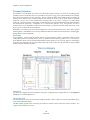
MAIN ANALYSIS WINDOW.......................................................................................................................................28
Sample File Tree ............................................................................................................................................28
Synthetic Gel Image and Electropherogram with Peak Table .......................................................................30
Report Table ..................................................................................................................................................33
MENU OPTIONS ....................................................................................................................................................34
File Menu .......................................................................................................................................................34
View Menu.....................................................................................................................................................35
Project Menu .................................................................................................................................................37
Applications Menu .........................................................................................................................................38
Tools Menu ....................................................................................................................................................39
Table of Contents
Help Menu .....................................................................................................................................................40
MAIN TOOLBAR ICONS ............................................................................................................................................40
CHAPTER 4 FRAGMENT SIZING STANDARDS................................................................................................. 43
SIZE TEMPLATE EDITOR ...........................................................................................................................................44
Procedure ......................................................................................................................................................46
Icons and Functions .......................................................................................................................................47
What to Expect ..............................................................................................................................................48
SIZE CALIBRATION CHARTS.......................................................................................................................................49
Procedure ......................................................................................................................................................51
Icons and Functions .......................................................................................................................................52
What to Expect ..............................................................................................................................................53
CHAPTER 5 PANEL EDITOR ........................................................................................................................... 55
OVERVIEW............................................................................................................................................................56
Panel List .......................................................................................................................................................56
Sample List ....................................................................................................................................................57
Overlay Trace.................................................................................................................................................57
Panel Table ....................................................................................................................................................59
PROCEDURE ..........................................................................................................................................................60
Pre-Defined Panels ........................................................................................................................................60
Custom Panel Creation ..................................................................................................................................61
Adjusting and Calibrating Panels ..................................................................................................................62
ICONS AND FUNCTIONS ...........................................................................................................................................63
Menu Options ................................................................................................................................................63
Toolbar Icons .................................................................................................................................................64
WHAT TO EXPECT ..................................................................................................................................................65
CHAPTER 6 REPORTS AND PRINTING ............................................................................................................ 67
REPORT TABLE ......................................................................................................................................................68
Allele List .......................................................................................................................................................68
Marker Table (Fragment) ..............................................................................................................................68
Bin Table (AFLP/MLPA) ..................................................................................................................................69
Peak Table .....................................................................................................................................................70
Allele Count ...................................................................................................................................................71
PRINT REPORT.......................................................................................................................................................72
Report Content Options .................................................................................................................................73
Icons and Functions .......................................................................................................................................74
SAVE PROJECT .......................................................................................................................................................74
CHAPTER 7 SPECIAL APPLICATIONS .............................................................................................................. 75
AMPLIFIED FRAGMENT LENGTH POLYMORPHISM (AFLP) ..............................................................................................76
Procedure ......................................................................................................................................................76
What to Expect ..............................................................................................................................................77
TERMINAL-RESTRICTION FRAGMENT LENGTH POLYMORPHISM (T-RFLP) .........................................................................79
Overview ........................................................................................................................................................79
Procedure ......................................................................................................................................................79
What to Expect ..............................................................................................................................................79
MULTIPLEX LIGATION-DEPENDENT PROBE AMPLIFICATION (MLPA) ................................................................................80
Overview ........................................................................................................................................................80
Procedure ......................................................................................................................................................82
Icons and Functions .......................................................................................................................................83
What to Expect ..............................................................................................................................................85
2
May 2012
Table of Contents
Reports and Printing ......................................................................................................................................89
Microsphere MLPA Analysis (Luminex)..........................................................................................................93
Methylation-Specific MLPA Analysis (MS-MLPA) ..........................................................................................95
HUMAN IDENTITY (HID) .......................................................................................................................................101
Procedure ....................................................................................................................................................101
What to Expect ............................................................................................................................................102
CODIS Report ...............................................................................................................................................102
PEDIGREE CHART .................................................................................................................................................103
Overview ......................................................................................................................................................103
Procedure ....................................................................................................................................................106
Icons and Functions .....................................................................................................................................108
What to Expect ............................................................................................................................................109
KINSHIP ANALYSIS ................................................................................................................................................110
Overview ......................................................................................................................................................110
Procedure ....................................................................................................................................................110
Icons and Functions .....................................................................................................................................111
Save and Print Report ..................................................................................................................................113
Importing Species Specific Allele Frequency and Mutation Rates ...............................................................113
DATABASE SEARCH: LOCATE DUPLICATE SAMPLES AND NEAREST RELATIVES....................................................................114
Overview ......................................................................................................................................................114
Procedure ....................................................................................................................................................114
Icons and Functions .....................................................................................................................................115
Save and Print Report ..................................................................................................................................116
Saving Genotypes from Two or More Multiplexes to the Database ............................................................117
PARENTAGE VERIFICATION FOR PURE BRED ANIMALS .................................................................................................118
Procedure: ...................................................................................................................................................118
Save Report .................................................................................................................................................119
QUANTITATIVE ANALYSIS .......................................................................................................................................120
Procedure ....................................................................................................................................................120
Icons and Functions .....................................................................................................................................121
What to Expect ............................................................................................................................................121
SINGLE NUCLEOTIDE POLYMORPHISM (SNP) ANALYSIS ...............................................................................................122
SNaPshot & SNuPE ......................................................................................................................................122
SNPlex ..........................................................................................................................................................127
SNPWave .....................................................................................................................................................129
SNP Analysis Reporting ................................................................................................................................130
MICROSATELLITE INSTABILITY (MSI) ........................................................................................................................131
Overview ......................................................................................................................................................131
Procedure ....................................................................................................................................................132
Icons and Functions .....................................................................................................................................132
What to Expect ............................................................................................................................................133
Reports and Printing ....................................................................................................................................134
PHYLOGENY CLUSTERING ANALYSIS .........................................................................................................................136
Detecting Euclidian Distance .......................................................................................................................139
Sub-cluster Report and Saving .....................................................................................................................140
Using Allele Bin Report from Merged Projects ............................................................................................140
TRISOMY DETECTION ............................................................................................................................................142
Overview ......................................................................................................................................................142
Procedure ....................................................................................................................................................143
Icons and Functions .....................................................................................................................................143
What to Expect ............................................................................................................................................145
Reports and Printing ....................................................................................................................................146
LOSS OF HETEROZYGOSITY (LOH) ...........................................................................................................................150
3
May 2012
Table of Contents
Overview ......................................................................................................................................................150
Procedure ....................................................................................................................................................151
Icons and Functions .....................................................................................................................................151
What to Expect ............................................................................................................................................152
Reports and Printing ....................................................................................................................................153
TILLING ANALYSIS ..............................................................................................................................................155
Overview ......................................................................................................................................................155
Procedure ....................................................................................................................................................156
Icons and Functions .....................................................................................................................................156
What to Expect ............................................................................................................................................157
Reports ........................................................................................................................................................158
HAPLOTYPE ANALYSIS ...........................................................................................................................................158
Overview ......................................................................................................................................................158
Procedure ....................................................................................................................................................159
Icons ............................................................................................................................................................162
ARMS/COMPARATIVE ANALYSIS FOR CYSTIC FIBROSIS ANALYSIS ..................................................................................162
Overview ......................................................................................................................................................162
Procedure ....................................................................................................................................................163
Icons and Functions .....................................................................................................................................163
What to Expect ............................................................................................................................................164
Reports and Printing ....................................................................................................................................165
CHAPTER 8 ADDITIONAL TOOLS ................................................................................................................. 167
BROWSE BY ALL COLORS .......................................................................................................................................168
OVERLAY VIEW....................................................................................................................................................168
MERGE PROJECTS ................................................................................................................................................169
Procedure ....................................................................................................................................................169
MACROMOLECULES ..............................................................................................................................................171
Procedure ....................................................................................................................................................171
FILE CONVERSION ................................................................................................................................................172
Procedure ....................................................................................................................................................172
FILENAME GROUP EDITOR .....................................................................................................................................172
Procedure ....................................................................................................................................................172
Icons and Functions .....................................................................................................................................172
OUTPUT TRACE DATA ...........................................................................................................................................174
Procedure ....................................................................................................................................................174
PROJECT COMPARISON .........................................................................................................................................174
Procedure ....................................................................................................................................................174
Icons and Functions .....................................................................................................................................175
CONVERT TXT TO BINARY......................................................................................................................................176
Procedure ....................................................................................................................................................176
EXPORT ELECROPHEROGRAM .................................................................................................................................176
Procedure ....................................................................................................................................................176
CHAPTER 9 USER MANAGEMENT ............................................................................................................... 177
OVERVIEW..........................................................................................................................................................178
PROCEDURE ........................................................................................................................................................178
USER MANAGER ..................................................................................................................................................178
HISTORY.............................................................................................................................................................179
SETTINGS ...........................................................................................................................................................179
EDIT HISTORY/AUDIT TRAIL ...................................................................................................................................179
INDEX .......................................................................................................................................................... 181
4
May 2012
Chapter 2 General Procedure
Chapter 1 Installing GeneMarker
Chapter 1 Installing GeneMarker
Computer System Requirements
Validation Version
Local Version
Network Version
Questions
5
May 2012
Chapter 2 General Procedure
Computer System Requirements
GeneMarker software has been tested and validated for various computer systems. The minimum system
requirements are:
Windows® PC
OS: Windows® XP, Vista, Windows® 7
Processor: Pentium® III, 1 GHz CPU
RAM: 512MB
Available hard disk space: 20GB
Intel® Powered Macintosh®
Parallels® desktop for Mac (Mac OS/virtual machine dependent) or Apple™ Boot Camp or VMware® Fusion
(Mac OS/virtual machine dependent)
RAM: 2GB
Available hard disk space: 20GB
Installation of GeneMarker is not supported on Linux or UNIX-based operating systems.
GeneMarker will only recognize PC file formats. To convert Macintosh file formats to PC file formats, please
download the ABI PRISM® 3100 Genetic Analyzer Conversion Utilities to convert Mac files to PC files at:
http://www.appliedbiosystems.com/support/software/3100/conversion.cfm
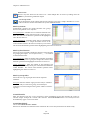
Validation Version
The validation or trial version of GeneMarker can be installed on as many computers as you wish. The trial
period expires 35 days after installation of the software.
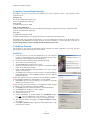
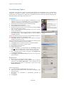
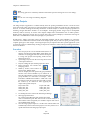
Installation
1.
Insert the SoftGenetics CD into the CD-ROM drive. If your computer
is not set to automatically open a CD, navigate to the optical or CDROM drive on the computer and open the directory.
2. Double-click the GeneMarker Setup executable file (EXE)
3. The Installation Wizard will launch
4. Click the Next button in the Welcome window
5. Read the SoftGenetics End User License Agreement and click the I Agree
button in the Read Me File window
6. Select “Install GeneMarker (Recommended)” in the Select Program
window and click Next
7. Click Next in the Destination Location window to install GeneMarker
in the default folder. Click the Browse button to choose a different
installation directory
NOTE: The default Destination Location for the GeneMarker program is
C:\ProgramFiles\SoftGenetics\GeneMarker\”version number”
8. Click Next in the Select Program Manager Group window to accept the
default Program Manager Group
NOTE: Changing the Program Manager Group default may affect program
operability. It is recommended to accept the default.
9. Click Next in the Start Installation window to install GeneMarker
10. Click Finish in the Installation Complete window
11. The Installation Wizard will close
12. Eject the SoftGenetics CD
13. Launch GeneMarker by double-clicking the GeneMarker desktop
icon OR open the Start menu and navigate to SoftGenetics →
GeneMarker, the version that was just installed → GeneMarker program
14. The Configure window will appear. Click Run Validation to launch
the software
15. If the Run Validation button is grayed-out this indicates the 35-day
trial period has expired.
6
May 2012
Chapter 2 General Procedure
Local-licensing Option
GeneMarker v2.00 and above supports text-based registration for the local-licensing option—no USB device,
dongle, key or hardware is required. This text-based registration ID is registered to one specific PC. If the
license needs to be transferred to a different PC, registration for that one license/PC must be inactivated first
before the software will be registered to the new PC.
Installation
1.
Insert the SoftGenetics CD into the optical or CD-ROM drive. If your
computer is not set to automatically open a CD, navigate to the
optical or CD-ROM drive on the computer and open the directory.
2. Double-click the GeneMarker Setup executable file (EXE)
3. The Installation Wizard will launch
4. Click the Next button in the Welcome window
5. Read the SoftGenetics End User License Agreement and click the I Agree
button in the Read Me File window
6. Select “Install GeneMarker (Recommended)” in the Select Program
window and click Next
7. Click Next in the Destination Location window to install GeneMarker
in the default folder. Click the Browse button to choose a different
installation directory
NOTE: The default Destination Location for the GeneMarker program is
C:\ProgramFiles\SoftGenetics\GeneMarker\ver#
8. Click Next in the Select Program Manager Group window to accept the
default Program Manager Group
NOTE: Changing the Program Manager Group default may affect program
operability. It is recommended to accept the default.
9. Click Next in the Start Installation window to install GeneMarker
10. Click Finish in the Installation Complete window
11. The Installation Wizard will close
12. Eject the SoftGenetics CD
13. Launch GeneMarker by double-clicking the GeneMarker desktop
icon OR open the Start menu and navigate to SoftGenetics →
GeneMarker, the version that was just installed → GeneMarker program
14. The Configure/Registration window will appear. Click Register Now
to register the local license
15. Click Register Local Text-based Key from the Choose Registration
Method dialog box
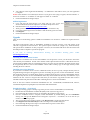
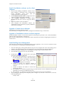
Registration
1.
2.
The Register Local Text-based Key window appears
If the computer GeneMarker is being installed on has an internet
connection, select Online Registration. If the computer does not
have an internet connection or is connected to a proxy server, select
Offline Registration.
Online Registration
A. Locate the Account and Password on the SoftGenetics CD.
B. Enter your Account, Password, and e-mail address information in the
appropriate fields
C. The Request Code information is automatically generated by
GeneMarker
D. Click Register
7
May 2012
Chapter 2 General Procedure
E.
Your software will be registered automatically. A confirmation e-mail will be sent to you once registration
is complete.
NOTE: Some characters can commonly be misread. If you get an error trying to register, check for number “1”
and lower case letter “L” or number “0” and upper case letter “O” confusion.
F. Launch GeneMarker and begin analysis
Offline Registration
A. Copy and paste the entire Request Code string and type your Account and
Password information from the SoftGenetics CD into the body of an e-mail
B. Send the email to [email protected]
C. The Registration ID will be sent to you (via email) within one business day
D. Copy and paste the Registration ID from the e-mail into the Registration ID field
E. Click Register
F. Launch GeneMarker and begin analysis
Upgrade
There are two local-licensing options available for GeneMarker v2.0 and above: USB-device required and textbased.
The legacy local-licensing option of GeneMarker available for previous versions (v1.97 and earlier) of the
software is supported for v2.0 and above. This option requires a USB device (dongle-, key-, hardware-based).
This option allows installation on many computers. However, the associated USB device must be inserted into
the USB port of the computer to operate the program.
If
you
wish
to
exchange
hardware-based
licensing
for
text-based
licensing
please
contact
[email protected].
Installing Over the Previous Version
If you choose to install the new version of GeneMarker over the previous version, you will need to choose the
same directory for installation. Several of the old files will be replaced with newer files. Other files that are not
present during installation but are created during analyses or by the user will remain in the folder and can easily
be recognized by the new version of GeneMarker. Please make a backup copy of the target directory before
installing the newer software.
Installing into a New Directory
If you choose to install the newer version in a different location, be sure to specify a unique directory name or
Program Manager Group for the upgrade to prevent overwriting any previous versions of GeneMarker. Several
files created by the users or created during analyses conducted by the previous version of GeneMarker will not
be recognized by the new version of GeneMarker unless they can be found in the directory of installation. If you
intend for the new version to recognize these files, then you will need to copy them from the older version’s
installation folder and paste them in the folder containing the new version of GeneMarker.
Some of the more common customized GeneMarker files are: GeneDB.mdb, GeneMarker.mdb, codis.ini,
CommentsTemplate.ini, ExpTemplates.ini, Panel folder and SizeStd folder.
Upgrade Procedure — Text-based
1.
2.
3.
4.
5.
6.
7.
8.
Before proceeding, prepare a backup copy of the previous version of GeneMarker (recommended)
Double-click the GeneMarker executable file (EXE) on the SoftGenetics Upgrade CD.
Proceed through the Installation Wizard as described in the Installation section above
Once the Installation Wizard is complete, launch GeneMarker by double-clicking the new GeneMarker
desktop icon OR open the Start menu and navigate to SoftGenetics → GeneMarker, the version that was just
installed → GeneMarker program
The Configure/Registration window appears. Click Register Now to register the local license
Click Register Local Text-based Key from the Choose Registration Method dialog box
Proceed through the Registration steps as described in the Registration section above
Launch GeneMarker and begin analysis
8
May 2012
Chapter 2 General Procedure
Upgrade Procedure — Hardware-based
1.
2.
3.
4.
5.
Before proceeding, prepare a backup copy of the previous version of GeneMarker
(recommended)
Ensure the GeneMarker USB key is inserted into the computer’s USB port
Double-click the GeneMarker executable file (EXE) on the SoftGenetics Upgrade CD.
Proceed through the Installation Wizard as described in the Installation section above
Once the Installation Wizard is complete, launch GeneMarker by double-clicking the
new GeneMarker desktop icon OR open the Start menu and navigate to SoftGenetics
→ GeneMarker, the version that was just installed → GeneMarker program
The Configure/Registration window appears. Click Register Now to register the local
license
7. Click Register Local Hardware Key from the Choose Registration Method dialog box.
The Register Local Hardware Key window appears
8. If the computer GeneMarker is being installed on has an internet connection, select
Online Registration. If the computer does not have an internet connection or is
connected to a proxy server, select Offline Registration.
9. Proceed through the Registration steps as described in the Online Registration or Offline
Registration section above
10. Launch GeneMarker and begin analysis
6.
Network-licensing Option
The network-licensing version of GeneMarker can be installed on any computer in a network configuration.
SoftGenetics uses the License Server Manager (LSM) to control the number of concurrent users accessing the
network-licensing option of GeneMarker v2.00 (and above). LSM uses text-based registration—no hardware is
required. Both software components are installed from the same EXE. The computer where License Server
Manager program is installed is considered the “Server” computer. Computers on the network other than the
Server are called “Client” computers.
Installing License Server Manager will require restarting the system to complete installation. Please save all
work and close all applications before installing LSM.
Install License Server Manager
1.
Insert the SoftGenetics CD into the optical or CD-ROM drive. If
your computer is not set to automatically open a CD, navigate to
the optical or CD-ROM drive on the computer and open the
directory.
2. Double-click the GeneMarker Setup executable file (EXE)
3. The Installation Wizard will launch
4. Click the Next button in the Welcome window
5. Read the SoftGenetics End User License Agreement and click the I
Agree button in the Read Me File window
6. Select “Install License Server Manager” in the Select Program
window and click Next
7. Click Next in the Destination Location window, Next in the Select
Program Manager Group window, and Next in the Start Installation
window to enter the LSM installation wizard
8. Click the Next button in the Welcome window
9. Read the SoftGenetics End User License Agreement and click the I
Agree button in the Read Me File window
10. Click Next in the Destination Location window to install LSM in the
default folder. Click the Browse button to choose a different
installation directory
NOTE: The default Destination Location for the License Server Manager
program is C:\ProgramFiles\SoftGenetics\License Server
11. Click Next in the Start Installation window to install License Server Manager
9
May 2012
Chapter 2 General Procedure
12.
13.
14.
15.
Select the Launch License Server Manager option and click Finish
Click OK in the Install window to restart the system.
The Installation Wizard will close and the system will restart
Eject the SoftGenetics CD
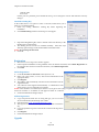
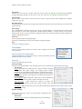
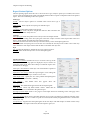
Register License Server Manager for GeneMarker Usage
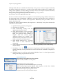
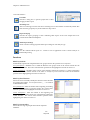
1. Open License Server from the System or Icon Tray by clicking the LSM icon
Note: A red star indicates the License server is not running. The icon with a
white star indicates the License Server is running properly.
2. Click OK in the dialog box to proceed with registering License Server
from the License Server Manager console.
3.
4.
5.
Select Register from the Help menu to activate the
Register Product window
Select GeneMarker from the Register Product Name
drop-down menu.
SelecIf the computer License Server is being installed on
has an internet connection, select Online Registration.
If the computer does not have an internet connection or
is connected to a proxy server, select Offline
Registration.
Online Registration
A. Locate the Account and Password on the SoftGenetics CD
B. Enter your Account, Password, and e-mail address information in the
appropriate fields
C. The Request Code information is automatically generated by
License Server
D. Click Register
E.
Your software will be registered automatically. A confirmation email will be sent to you once registration is complete.
NOTE: Some characters can commonly be misread. If you get an error
trying to register, check for number “1” and lower case letter “L” or
number “0” and upper case letter “O” confusion.
F. Restart License Server to apply the registration information.
Offline Registration
G. Copy and paste the entire Request Code string and type your Account
and Password information from the SoftGenetics CD into the body of an
e-mail
H. Send the email to [email protected]
I. The Register ID will be sent to you (via email) within one business day
J. Copy and paste the Registration ID from the e-mail into the Register ID
field of the Offline Registration tab
K. Click Register
10
May 2012
Chapter 2 General Procedure
Install GeneMarker software on the client
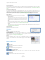
computer
1.
2.
3.
4.
5.
Proceed with installing GeneMarker software on the
client computer as described in the “Local-licensing
Option, Installation” section above until the
Configure/Registration window appears
Click Configure Network Client to configure the client
software to contact License Server Manager
Click Configure Connection to License Server
Manager from the Choose Network Configuration dialog
box
Input Server Name or Server IP Address
Click Configure and GeneMarker software will
automatically open if connection is properly established
and a license is available.
Upgrade of License Server Manager
Activate the License Server Manager console
Proceed with step 3 of “Register License Server Manager for GeneMarker Usage” section above
Upgrade of GeneMarker software on client computer
Install GeneMarker software on the client computer by following the procedure in the “Install GeneMarker
software on the client computer” section above.
If the network configuration has not changed the software should activate without configuring the IP address of
License Server.
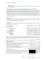
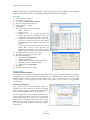
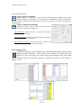
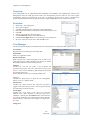
Install NetDog Server Management
The following are instructions for installing the NetDog Server application. See Local Version Installation section
above for instructions on installing the GeneMarker program.
1.
2.
3.
4.
5.
Insert the NetDog Key (USB/parallel hardware key) into the computer that will run the NetDog Server
software. The computer may be any client computer on your network that runs Microsoft Windows.
Launch the setup file of NetDog Server (/NetDog Server Setup/setup.exe) and install the server.
After installation, NetDog Server starts automatically.
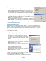
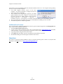
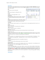
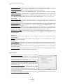
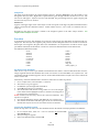
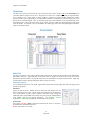
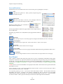
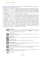
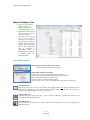
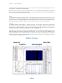
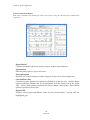
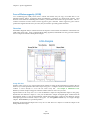
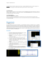
Double-click the
icon on the task bar to open up the
NetDogServer Management application.
A. The section in the figure that A is referring to shows
that the NetDog Server is able to detect the NetDog.
If it is unable to detect the NetDog, it will display
(please refer to the section about
installing the NetDog key to correct this).
B. Column B indicates the maximum number of
concurrent users that are allowed to access the
software.
C. Column C indicates the number of current users
running the software.
D. The “Module 0” row indicates programs being used in the network version of Mutation Surveyor (Not
applicable if you do not have Mutation Surveyor).
E. The “Module 1” row indicates programs being used in the network version of GeneMarker.
After installing the NetDog Server Program, please configure any firewalls on the server to allow the
following default ports:
TCP/IP: 4587
11
May 2012
Chapter 2 General Procedure
UDP/IP: 4587
IPX: 17799
If other ports are preferred, please launch the NetDog Server Management console and make the necessary
changes.
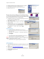
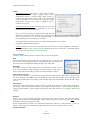
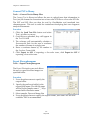
Install the NetDog Key
In the toolbar, there is an option to Install or Uninstall, which allows you to
delete or re-install the NetDog.
1. Delete any existing “Mutation” NetDog Key before beginning the
installation.
2. Click Install NetDog and the Install NetDog box will appear
3.
Import the NDogINst.cfg file, which is located in the same directory as the
NetDog Server setup package.
4. The NetDog Server can also be installed manually. Select the Input
Manually option and type in the Serial Number and Product name.
NOTE: Do not change the Password.
5. Click OK
Registration
1.
2.
3.
The Network Version Registration window appears
If the computer GeneMarker is being installed on has an internet connection, select Online Registration. If
the computer does not have an internet connection, select Offline Registration.
Click Next
Online Registration
A. Locate the Account and Password on the SoftGenetics CD.
B. Enter your E-mail Address, Account, and Password information in the
appropriate fields
C. Click Register
D. The USB key will automatically load the User ID information into the
registration field.
E. Your software will be registered automatically. A confirmation e-mail
will be sent to you once registration is complete.
NOTE: Some characters can commonly be misread. If you get an error trying to register, check for number “1”
and lower case letter “L” or number “0” and upper case letter “O” confusion.
F. Launch GeneMarker and begin analysis
Offline Registration
A. Copy and paste the entire User ID string and type your Account and
Password information into the body of an e-mail.
B. Send the email to [email protected].
C. The Registration ID will be sent to you (via email) within one business
day.
D. Copy and paste the Registration ID from the e-mail into the Registration
ID field.
E. Click Register
F. Launch GeneMarker and begin analysis
Upgrade
12
May 2012
Chapter 2 General Procedure
The upgrade version of GeneMarker Network should be installed on the server – the computer running NetDog
Server – as well as all client computers.
1. First install upgrade network version on the server
computer. You will be prompted to configure the network
(enter server name or IP address).
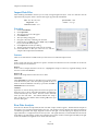
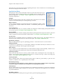
2. After installing and configuring the upgrade you should
update NetDog on the server computer. To do this, launch
the NetDog Upgrade tool. NetDog Update can be accessed by
going to Start menu → All Programs → SoftGenetics →
GeneMarker (Network) → NetDogUpdate. It is located in the same directory as the GeneMarker program.
3. The Confirm dialog box will appear if the versions of GeneMarker and NetDog are not consistent.
4. Click Yes and proceed to software registration.
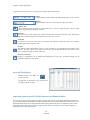
Additional User Licenses
If you are interested in purchasing additional user licenses, please launch the upgrade tool (NetDogUpdate.exe)
that is located in the GeneMarker directory.
1. Click the Produce Request String button.
2. Copy the string in the text field and paste it into an email addressed to [email protected] for further
order information. Another encrypted string of characters will be emailed to you.
3. Copy and paste the string into the second text field.
4. Click Update and the number of licenses in NetDog will automatically be updated.
5. Re-install the NetDog Server following the Installation section above.
Questions
If you have any questions during installation, setup, or program operation, please contact us at (814) 237-9340
OR (888) 791-1270 OR email us at [email protected]
13
May 2012
Chapter 2 General Procedure
14
May 2012
Chapter 2 General Procedure
Chapter 2 General Procedure
Chapter 2 General Procedure
Import Data Files
Raw Data Analysis
Process Data
Adjust Analysis Parameters
15
May 2012
Chapter 2 General Procedure
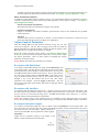
Import Data Files
After installing GeneMarker software you are ready to begin fragment analysis. First, raw data files must be
uploaded to the program. Below is the list of file types supported by GeneMarker.
ABI - .fsa, .abi, .ab1, .hid
MegaBACE - .rsd
Beckman-Coulter - .esd
Spectrumedix - .smd
Generic - .scf, .sg1
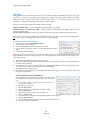
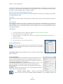
Procedure
1.
2.
3.
4.
5.
6.
7.
Launch GeneMarker
Click Open Data
The Open Data Files box will appear
Click Add button
The Open dialog will appear
Navigate to directory containing raw data files
Select all files by CTRL+A or use CTRL and/or SHIFT
keys to select individual samples
8. Click Open button in the Open dialog
9. The files selected will appear in the Data File List field
10. Click OK button in the Open Data Files box and the
samples will be uploaded to GeneMarker
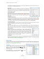
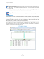
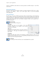
Features
There are several features available in the Open Data Files box to make data upload easier.
Add…
Used to locate and select raw data files for upload. Click the arrow button next to the Add button to see the four
most recently accessed directories.
Remove
Used to remove samples from the Data File List. Highlight the sample to remove by single left-clicking it in the
Data File List then click Remove.
Remove All
Removes all sample files from the Data File List field.
Add Folder…
Click Add Folder to upload raw data files from a specific folder
in the file directory tree. Click the Default hyperlink to choose a
folder to which GeneMarker will always open when the Add or
Add Folder buttons are clicked.
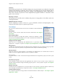
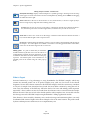
Channels
Opens the Set Channels dialog with 4 and 5-color tab options and
allows the user to choose from ABI, MegaBACE, and BeckmanCoulter standard dye color orders. The user can also manually
enter dye color and name. The default channel color setup is
ABI. Set the dye color channels before clicking OK in the Open
Data Files dialog box.
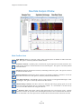
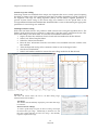
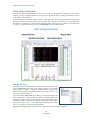
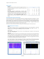
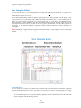
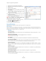
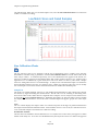
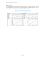
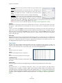
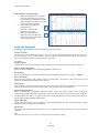
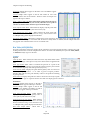
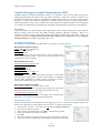
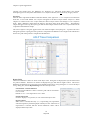
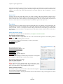
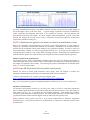
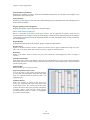
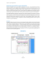
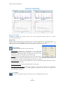
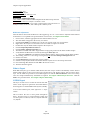
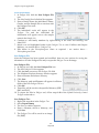
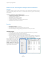
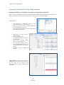
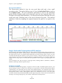
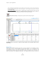
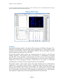
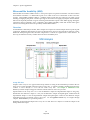
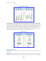
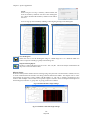
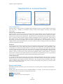
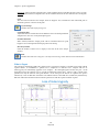
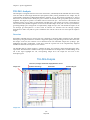
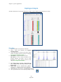
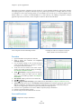
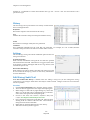
Raw Data Analysis
Once the raw data files are uploaded, the Raw Data Main Analysis window appears. Double-click the samples in
the Sample Tree to open the individual Raw Data Traces. The Synthetic Gel Image displays the unprocessed data in
a traditional gel format with larger fragments located on the right. The Electropherograms display fluorescent
signal intensities as a single line trace for each dye color. The signal intensities, recorded in Relative Fluorescent
Units (RFUs), are plotted along a frame scale in the Raw Data Analysis window with fragment mobility from right
to left. The smallest size fragments are on the far left of the trace.
16
May 2012
Chapter 2 General Procedure
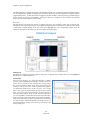
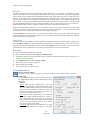
Raw Data Analysis Window
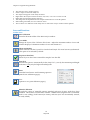
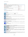
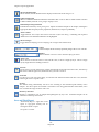
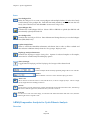
Main Toolbar Icons
Spike Removal: Removes peaks from voltage spikes caused by micro-air bubbles or debris in the laser
path. This option is selected by default in the Run Wizard.
Saturation Correction: A synthetic peak is created based on peak shape before and after saturation. The
results of these will be less accurate than that of non-saturated peaks. This option is selected by default
in the Run Wizard.
Smooth: This function smoothes the baseline by eliminating smaller noise peaks. This option is selected
by default in the Run Wizard.
Baseline Subtraction: Selecting this option will remove the baseline completely so that the Y-axis will be
raised above the noise level. This option is selected by default in the Run Wizard.
Auto Pull-up Removal: Automatically removes peaks caused by wavelength bleed-through to other
wavelengths. This option is selected by default in the Run Wizard.
Manual Pull-up Correction: This allows the user to manually adjust larger pull-up peaks in case the
Auto Pull-up Removal function has not corrected the problem. It is recommend to de-select Pull-up
Correction in the Run Wizard when using this function.
2nd Derivative Trace: This feature reduces high background noise and sharpens peaks. Baseline
fluctuation caused from dye blobs or the DNA template in PCR can also be reduced with this function.
It is recommended to de-select Spike Removal in the Run Wizard when this function has been activated.
17
May 2012
Chapter 2 General Procedure
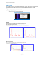
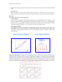
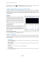
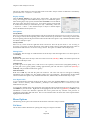
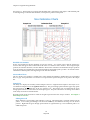
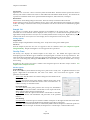
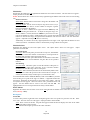
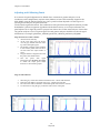
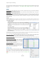
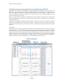
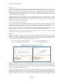
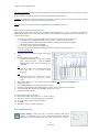
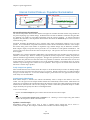
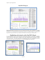
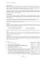
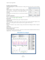
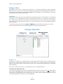
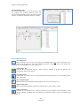
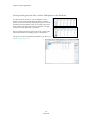
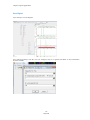
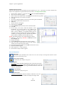
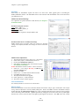
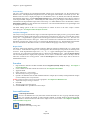
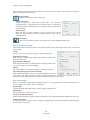
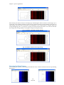
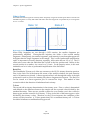
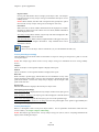
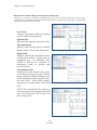
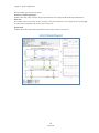
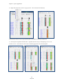
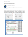
What to Expect
The raw data correction icons can be selected individually in the Raw Data Analysis window. The images below
demonstrate how the data will look before (left image) and after (right image) the parameter is applied.
Range
AutoRange - Analyzes from 0 to end of trace for size call
Manual Range – user-defined range
Right-click in gel image and select Get Start Point
Smooth
Fourier frequency transformation (FFT) to determine frequency domain
Use only top 40% of lowest frequencies
Smoothing broadens peaks and therefore you can lose resolution
Enhanced Smooth - Same as Smooth but use only top 20% of lowest frequencies
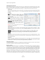
Baseline Subtraction
Use 20% of lowest intensities (to the right of the beginning of the range)
Looks at trace in 500-600 frame sections
18
May 2012
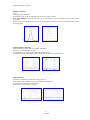
Chapter 2 General Procedure
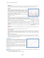
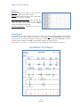
Pullup Correction
Ax=B
A being the major coefficient
Input matrix or use single dye adjustment up to 0.20 for small corrections
When Manual Pullup correction is chosen, a .txt or .mtx matrix file can be uploaded and used to deconvolute
dye colors.
NOTE: De-select automatic Pullup Correction in the Run Wizard Data Process box if a manual matrix correction
has been applied.
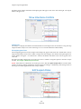
Saturated Peak Correction
ABI instrument saturated peaks are typically >8000 RFU
The top of a saturated peak looks split
A small pullup peak may be present under the saturated peak
GeneMarker takes the small pullup peak and adds it to the split in the saturated peak
Spike Removal
Caused by overheating of camera chip, voltage spike, etc
Spikes usually only 1-2 frames wide; peaks usually 5-10 frames wide
Create a first derivative trace of the raw data
Spikes are the 1st DT outliers (3-5 sigma)
19
May 2012
Chapter 2 General Procedure
Second Derivative Trace
(A1-A2)-(A2-A3) = A1+A3-2(A2)
Use when you have a fat base to your peaks (ex. Dye blob under peak, etc)
NOTE: Do not use 2nd DT with Spike Removal because real peaks look like spikes.
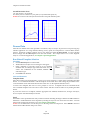
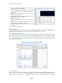
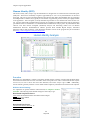
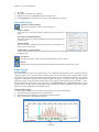
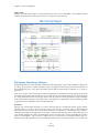
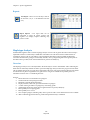
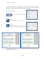
Process Data
After the raw data files have been uploaded to GeneMarker, they are ready to be processed. The processing step
includes application of a sizing standard, filtering of noisy peaks, and comparison to a known allelic Panel if
desired. GeneMarker combines all these steps in one simple tool called the Run Wizard. To access the Run
Wizard simply click the Run Project icon in the main toolbar. The example below is for a basic fragment
analysis. For advanced applications, see Chapter 7 Special Applications.
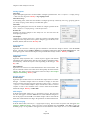
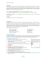
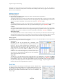
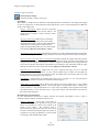
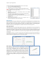
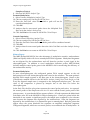
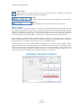
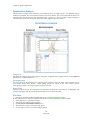
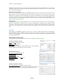
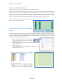
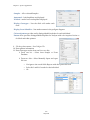
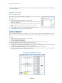
Run Wizard Template Selection
Procedure
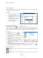
1.
2.
3.
4.
Click the Run Project icon in the toolbar.
The Run Wizard Template Selection dialog box will appear.
Select a template (a previously saved set of size standard,
standard color, and analysis type named for future use), OR
select a new combination of size standard, standard color,
and analysis type.
Click Next when finished.
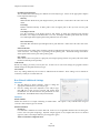
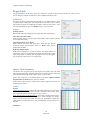
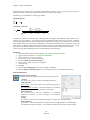
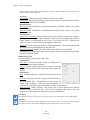
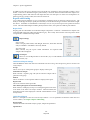
Icons and Functions
Template Name
Select from existing pre-made templates or create your own by entering a Template Name and clicking the Save
button. To save the Run Parameters with the template use the ‘Back’ arrow after setting the parameters in the
second and third screens of the Run Wizard. Then select ‘Save’ on the Tepmalte Selection screen.
To create a new template, click Select an existing template or create one. A template can also be selected from the
list of available templates in the left section of the window and then saved for future use by clicking the Save
button.
If you do not want to use a template, select the appropriate size standard, standard color, and type of analysis;
Use last template will automatically be selected.
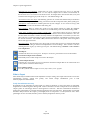
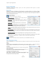
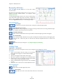
Panel
GeneMarker comes preloaded with many common kit Panels including Promega’s MSI kit and MRC Holland’s
MLPA kits. Additional Panels can be imported by selecting the Open Files icon next to the Panel field. A custom
Panel can be created in the Panel Editor tool. See Chapter 5 Panel Editor.
NOTE: It is recommended to size the data prior to selecting a Panel for comparison. Select NONE in the Panel
field for the first Run Wizard data process action.
20
May 2012
Chapter 2 General Procedure
Panel Editor: A Panel can be selected from any available from the drop-down menu, or can be viewed
and selected by clicking the Panel Editor icon.
Import a Panel: If a Panel cannot be found in the Panel Editor tool, it can be imported by clicking on the
Import a Panel icon.
Size Standard
GeneMarker comes preloaded with many common size standards including GeneScan 500 and LIZ600. A
custom Size Standard can be created by selecting the Size Template Editor icon next to the Size Standard field. See
Chapter 4 Fragment Sizing Standards.
Size Template Editor: This allows the user to check sample files against a selected size standard,
modify and save the size standard for future use, or create a new size standard.
Standard Color
Select the dye color which contains the internal lane standard.
Analysis Type
Selecting an analysis type will set the options in the two subsequent boxes of Run Wizard (Data Process and
Additional Settings) to the optimal settings for the analysis type selected. See Chapter 7 Special Applications.
Run Wizard Data Process
Procedure
5.
6.
The Data Process window of Run Wizard will activate. This
allows the user to select the peak filtering parameters. The
settings will vary depending on the Analysis Type selected.
Select the appropriate analysis settings in the Data Process
window and click Next to continue.
Icons and Functions
Raw Data Analysis
Auto Range (frame)
The range in camera frames will automatically find the processable data range. If Auto Range is not selected,
manually enter the start and end frame numbers of the data set for analysis.
Intensity Coefficients: Allows for manual correction of excessive bleedthrough peaks; best used for experiments with one-color analysis.
Smooth
Smoothes the baseline by eliminating smaller noise peaks.
Enhanced Smooth
This feature is used only in cases where the data is extremely difficult to
analyze and cannot be corrected with the Smooth function.
Peak Saturation
The software will analyze saturated data points by creating a synthetic estimate of the peak shape based on
the curves prior to saturation. The results will be less accurate than that of non-saturated peaks.
Pull-up Correction
This function removes peaks caused by wavelength bleed-through to other wavelengths. The function
should be disabled if a Manual Pull-up Correction was used in the Raw Data Analysis window.
Baseline Subtraction
This function removes the baseline completely so that the Y-axis will be raised above the noise level.
Enhanced Baseline Subtraction
21
May 2012
Chapter 2 General Procedure
This function should be applied for samples that have a high baseline, especially in the 40-80 bp mini-STR
range.
Spike Removal
Removes peaks from voltage spikes caused by micro-air bubbles or debris in the laser path. Spikes are
typically less than a base-pair wide. Do not select Spike Removal when 2nd Derivative Trace has been applied.
Size Call
GeneMarker offers three sizing methods:
Local Southern
Used in most genotyping software applications and is recommended for most analyses. This
method is based on the idea that smaller size fragments run faster. Plot a size v. time graph and
overlay a size v. 1/time graph to determine linear trace. (Southern, E.M. “Measurement of DNA
Length by Gel Electrophoresis.” 1979. Analytical Biochemistry. 100, 319-323).
Cubic Spline Method
Cubic Spline is offered as an alternative method that may be more appropriate for some data.
This method uses a cubic equation to connect known points on the size v. time graph. An
example of a cubic equation: ax3+bx2+cx+d. (The Astrophysical Journal. December 1, 1994. 436,
pages 787-794.)
Local Southern Method
Cubic Spline Method
Large Size AlgorithmGeneMarker’s new algorithm provides accurate, linear sizing of the data using
a DNA derivative migration time correction to large DNA fragments. Selecting Large Size algorithm
enables accurate sizing from small to large (30-1400) base pair fragments. The peak area in base space
accurately determines the copy numbers because the peak area normalization is much less variable
than that of the height normalization. The peak width is less than 1 bps for all fragments less than 1k.
22
May 2012
Chapter 2 General Procedure
Custom Large Size Calling
Some large custom size standards have unique size fragments that are not evenly spaced; requiring
the ability to change some of the parameters in the large size calling algorithm to provide a best fit to
the fragments. The large size calling algorithm (above) will use analyst supplied parameters to
provide accurate linear sizing of the custom large size standard. Use the spread sheet in the
C:ProgramFiles:SoftGeneticsGeneMarkerSize Standard folder to assist in determining the appropriate
parameters for custom large size standards.
Flanking Peak Size Calling
With some non-linear data it is not possible to make a best fit curve using the algorithms above. The
flanking peak method uses the fragments on either side of the data peak to interpolate the size. This
allows size calling of non-linear data. To create the size standard for this method:
1. Import raw data files and Select None for Panel and Size Standard in the Run Wizard
2. Select Tools Size Template Editor
3. Select File New Size Standard
4. Enter the ‘Size’ information from the run without a size standard in the Size column of the
Size standard
5. Enter the Expected size bp; in the comments column as seen in the figure below
6. Save the size standard file
7. Select Local Southern method to activate this size calling method in the Run Wizard
Allele Call
The Allele Call section allows the user to set allele calling range,
detection thresholds and filters.
Auto Range
The software will automatically display the processable data range
for each lane.
Manual selection of Range
To select a specific analysis region, de-select Auto Range and input
the desired base pair range. Additionally, if automatic size call
fails due to high saturation, de-select Auto Range and manually
input the required data range.
23
May 2012
Chapter 2 General Procedure
Peak Detection Threshold
The recommended initial settings are different for each analysis type. Please see the appropriate chapters
for the required analysis type.
Intensity
Minimum RFU threshold of peak height used for peak detection. Peaks below this value will not be
called.
Percentage
Relative minimum intensity of allele peaks to the 5th highest peak in the dye color used for peak
detection.
Local Region Percent
Uses the percentage of the highest peak for that marker to define the minimum peak detection
threshold. For example, if the threshold is set to 33%, the height of all allele peaks must reach at least
33% of the height of the highest peak in that particular locus to be called.
Max Call Intensity
Maximum RFU threshold of peak height used for peak detection. Peaks above this value will not be
called.
Stutter Peak Filter
Forward and reverse stutter peaks commonly caused by PCR/chemical reactions can be removed using the
Stutter Peak Filter. The settings are in percentage of the primary peak. The default settings will remove
stutter peaks within 2.5 base pairs of the primary peak.
Plus A Filter
When selected, the second peak of a split peak (one basepair spacing between two peaks) will not be called.
Deselect to call both peaks separately.
Load Default
Recalls any settings previously saved by the user. If there are no user-saved settings, the program loads the
default settings for that particular analysis type.
Save Default
Saves any settings defined by the user that is different from the default. These settings can be recalled for
consistency of analysis on similar data sets.
Run Wizard Additional Settings
Procedure
7.
8.
The Run Wizard is almost complete. Enter or change the
appropriate information for your analysis type.
Once the settings have been adjusted to your analysis type,
click OK and a Data Processing window will appear while
GeneMarker sizes the data based on the parameters set in the
Run Wizard. Click OK when the analysis has finished.
Functions
Allelic Ladder
Permits the selection of a sample containing an allelic ladder. This option is only available when Fragment
(Animal) or HID analysis types are selected.
Allele Evaluation
Peak Score
User-definable confidence level of the allele call. Peak score is an algorithm that takes into account signalto-noise ratio and peak morphology. Rejected samples appear in red, samples that need to be checked
appear in yellow, and samples that have passed appear in green.
AFLP Unconfidence at Rightside Score
24
May 2012
Chapter 2 General Procedure
Available only when AFLP Analysis method is chosen. When selected the user can enter the minimum score
at which a peak to the right of the main peak will be called. See Chapter 7 Special Applications - AFLP.
MLPA Normalization Method
Available only when MLPA Analysis method is chosen. Two normalization methods are available to correct for
variations of PCR efficiencies from small to large DNA fragments or from sample to sample. See Chapter 7
Special Applications MLPA.
Internal Control Probe Normalization
The traditional method of normalization using the control probes.
Population Normalization
Unique to GeneMarker, this method normalizes peak intensities based on the statistically most probable
median intensities.
Advanced
Available when Population Normalization is selected. Advanced Population Normalization is meant to be used
when more than half of the probes are deletions or duplications.
Adjust Analysis Parameters
After the clicking OK in the Run Wizard Additional Settings box, the Data
Processing box appears. The raw data is being processed and sized, then the
filtering parameters are applied, and finally a Panel is applied (if selected). Click
OK in the Data Processing box when analysis is complete.
Review the results in the Main Analysis window. See Chapter 3 Main Analysis
Overview. If you notice many false positive peak calls, you may need to adjust
the analysis parameters. There are three options for adjusting the analysis
parameters as discussed below.
NOTE: Manual edits will be lost when data is re-analyzed.
Re-analyze with Run Wizard
To re-analyze with the Run Wizard tool, simply click the Run Project icon
in the main toolbar. The Run Wizard will launch and the most recently
selected parameters will be displayed. Adjust parameters as necessary and
click OK in the Run Wizard Additional Settings box. The Use Old Calibration
box will appear with the option to Call Size Again. Only select Call Size
Again if the Run Wizard Template Selection Size Standard selection was
changed or any of the Run Wizard Data Process Raw Data Analysis
parameters were changed. Click the Apply to All button. The Data
Processing box will appear again and the data will be re-analyzed with the
new parameters.
Re-analyze with Auto Run
To re-analyze with Auto Run, first select Project → Options. The Project Options Settings box will appear. This
box offers all the same parameters settings as are available in the Run Wizard. Use the tabs to view the Template
Selection, Data Process, and Additional Settings boxes. Click OK when finished. Next, select Project → Auto Run.
The data will be re-analyzed with the new parameters.
NOTE: The Additional Settings Allele Evaluation Peak Score parameters can be changed in the Project Options
Settings box and will be applied to the data without having to re-analyze the data with Run Wizard or Auto Run.
Re-analyze Individual Samples
To re-analyze an individual sample, dye color, or marker, click the Call Allele icon in the main toolbar. The
arrow next to the icon opens the drop-down menu with additional options. Click an option from the drop-down
and the Recall Allele box will appear. Adjust parameters as
necessary and click OK. The new parameters will be applied.
All Samples
Applies the new parameter settings to all samples in the
dataset – similar to Run Wizard and Auto Run.
25
May 2012
Chapter 2 General Procedure
Open Samples
Applies the new parameter settings only to samples that are checked in the Sample File Tree.
Current Sample
Applies the new parameter settings only to the sample highlighted in the Sample File Tree.
Call the Dye
Applies the new parameter settings to the dye selected in the Recall Allele → Call Allele by Dye field.
Call the Marker
Applies the new parameter settings to the marker selected in the Recall Allele → Call Allele by Marker field.
26
May 2012
Chapter 3 Main Analysis Overview
Chapter 3 Main Analysis Overview
Chapter 3 Main Analysis Overview
Main Analysis Window
Menu Options
Main Toolbar Icons
27
May 2012
Chapter 3 Main Analysis Overview
Main Analysis Window
The main window of GeneMarker has an easy to use layout. The sample files are displayed on the left, the
Synthetic Gel Image is displayed at the top, Electropherograms appear below the gel image, and the Report Table is
on the right side of the window.
To resize the frames in the Main Analysis window, simply place the cursor over the partitions that separate the
Synthetic Gel Image/Electropherogram/Sample File Tree/Report Table. The cursor will change to a two-headed arrow
bisected by two vertical lines. Hold down the left mouse button and drag the gray vertical line in the direction
you wish. To open and close the frames, use the Show/Hide icons in the main toolbar.
Main Analysis Window
Sample File Tree
The Sample File Tree of the main analysis window contains two folders. The
first is the Raw Data folder which, when expanded, displays a list of all the
dataset samples. When a sample is double-clicked its preprocessed
electropherogram trace will appear in the Raw Data Analysis window. See
Chapter 2 General Procedure.
The second folder, Allele Call, also contains a list of all the samples, but
when the filename is double-clicked the sample’s electropherogram trace
appears in the Main Analysis window with all sizing information and allele
call filtering applied. The Allele Call folder also flags each sample with a
green sheet, yellow sheet or red strike-through indicating size calling
success. See Chapter 4 Fragment Sizing Standards.
Right-click the sample filename in the Raw Data or Allele Call folder to see additional options.
28
May 2012
Chapter 3 Main Analysis Overview
Sorting Options
Select Page
Opens electropherogram traces for the number of samples specified in the View → Preference → Display Settings
→ Max Chart # In Page field. Hot Key = Page Up/Page Down
Select Next Group
In descending order, selects the same number of samples previously selected by Select Page, grouping options
(see Sample Grouping section below) or double-click option.
Select Max
Opens electropherogram traces for the number of samples specified in the
View → Preference → Display Settings → Max # Open Charts.
Deselect All
Unselects all selected samples in the Sample File Tree list and closes the
electropherogram traces.
Sort Samples
Opens the Sort Sample Options box. Select First, Second, and Third Order
sorting from the drop-down menu options Sample Type, File Name, Lane
Number, Well ID, and Size Score. Hot Key = F3
Search Options
Search File
Opens the File Search box. Enter any part of a filename to search for the sample in the list. Click the Search
button. Left-click and use CTRL or SHIFT key to highlight samples then click the Open Selected button. The
electropherograms of the selected samples will open in the Main Analysis window. Hot Key = CTRL+F
Sample Information
Sample Info
Opens the Sample Information box. A list of Properties appears and includes
information like; Sample Name, Well ID, Lane Number, Instrument Name,
and Chemistry. The list of Properties varies depending on the file type. Hot
Key = F2
Edit Comments
Opens the Edit Comments box. Enter information in the Comments field. The
last ten comments will be stored and can be subsequently selected for future
samples. The Sample Comments will appear on the Print Report. See Chapter
6 Reports and Printing. Hot Key = F4
Disable Samples
Disable Sample
Opens the Input Disable Reason box and marks the sample with a red strikethrough. A disabled sample cannot be selected for display in the Main
Analysis window and will not appear in the Report Table if View → Preference
→ Options → Show Disabled Samples in Report is deselected. Select a Comment
Template or enter a new comment in the Comments field and click OK to
disable the sample. Hot Key = CTRL+DEL
Add Samples
From the main toolbar, select Project → Add Samples to Project. The Open Data
Files box will appear. Click the Add button to select additional samples to
add to the project and click OK. The added samples will be sized and the
allele calls will be filtered according to the parameters set in the Run Wizard.
Sample Grouping
From the main toolbar, select Project → Apply Sample Grouping. The File Name Group Editor tool will appear (See
Chapter 8 Additional Tools). Select Group and Control identifiers and click Match. Click OK to apply the
matched groups. Group numbers will appear next to the filenames in the Sample File Tree. Use the Select Next
29
May 2012
Chapter 3 Main Analysis Overview
Group right-click menu option OR CTRL+PageUp/Down to open samples in a group. To disable the Sample
Grouping feature, go to View → Preference → Others and uncheck Enable Sample Grouping.
Synthetic Gel Image and Electropherogram with Peak Table
The Synthetic Gel Image and Electropherogram displays are associated in the Main Analysis window. Both display
the fragment information in a visual form. When GeneMarker is initially launched, all dye colors are displayed
in the Synthetic Gel Image and Electropherogram at once. Single left-click the Show Color icon in the main toolbar
to cycle through the dye colors or use the Show Color drop-down menu to disable individual colors or
Show/Hide All colors.
Navigation
Zoom In/Out
In the Synthetic Gel Image or the Electropherogram, hold down
the left mouse button and drag a box from upper left to
lower right around the area you would like to zoom in on.
To zoom back out, hold down the left mouse button and
drag a box in the opposite direction from lower right to
upper left. The user may also use the Zoom icons in the
main toolbar to zoom in and out. The main analysis
window also allows the user to manually set the x and y
axis with the Set Axis icon.
Horizontal Movement
The Synthetic Gel Image and the Electropherogram are
synchronized to allow the user to view both images at once.
To move the images in the horizontal direction, use the top
slider bar (below the toolbar) to scroll the image in either
direction, or hold down the right mouse button and drag
the trace right or left.
Marker/Locus Specific Viewing
To scroll through individual markers/loci, select a marker from the Marker drop-down list in the main toolbar.
To view subsequent markers, use the Up/Down Arrow keys.
Synthetic Gel Image Features
The Synthetic Gel Image displays all samples in the dataset vertically. The direction of fragment mobility is
horizontal with the small size fragments on the left and the larger fragments on the right so that the gel aligns
with the electropherogram trace display. Move the mouse pointer over the Synthetic Gel Image to reveal the
sample lane filename.
Image Utilities
Click the Image Utilities icon in the upper left corner of the Synthetic Gel Image. A fly-out menu appears
with the following options:
Copy to Clipboard
Copies the Synthetic Gel Image to the Windows clipboard for pasting into other applications such as
Microsoft PowerPoint.
Save Image
Allows the user to save the Synthetic Gel Image as a BMP image file.
Show in Window
Opens a separate window containing the Synthetic Gel Image. The separate window can be maximized for
closer gel image inspection.
30
May 2012
Chapter 3 Main Analysis Overview
Image Display
Intensity
Move the Intensity slide bar, located in the upper left corner of
the Synthetic Gel Image, up and down to adjust the intensity of the
fragments displayed.
Grey-Scale
Go to View → Preference → Display Settings → Gel Image. Select
Gray for Single Dye to change the single dye Synthetic Gel Image
to black and white when only a single dye color is selected (when
multiple dye colors are selected the fragments will appear in their
respective colors). Click the Background in White option to
reverse the black and white exposure for single dye color gel
images.
Electropherogram and Peak Table Features
The Electropherogram displays fluorescent signal intensities from capillary electrophoresis instruments as a single
line trace for each dye color. The signal intensities are recorded in Relative Fluorescent Units (RFUs) which are
plotted along the y-axis. Along the x-axis are the basepair sizes of the fragments. The frame units plotted along
the x-axis in the original Raw Data Analysis window are converted to basepair size units as defined by the Size
Standard selected and the Internal Lane Standard (ILS) of the individual samples. Fragment mobility is from
right to left with the smallest size fragments on the far left of the trace.
The Peak Table contains information about the called peaks currently displayed in the Electropherogram.
Electropherogram Trace Display
Range
The basepair size range (x-axis) is as set in the Run Wizard Data Process Allele Call options box. The RFU
range (y-axis) is variable and will re-adjust according to the maximum peak height in the trace. To
manually set x and y-axis ranges, use the Set Axis icon in the main toolbar.
Cursor Locator
The x and y-axis position of the mouse pointer in the electropherogram is displayed in the upper right
corner of the electropherogram.
Allele Call
If a Panel is applied to the data, then grey horizontal bar Markers will appear above the electropherogram
indicating locus ranges. Bin ranges appear as dye-colored brackets above and below the sample trace. Allele
Labels appear below the electropherogram and are associated with the center of each called peak which is
also marked by a light grey vertical line in the electropherogram. If a Panel is not applied, then Allele Labels
for called peaks will only indicate the basepair size of the peak.
The red horizontal line (seen here in the figure on the right) is to alert analysts to trends in the data. These
areas of the data have a more elevated baseline or noise-to-signal ratio (often associated with poorly
resolved peaks) than the nearby regions of the trace which sometimes masks very minor peaks.
31
May 2012
Chapter 3 Main Analysis Overview
Peak Table
The Peak Table can be displayed below the Electropherogram by clicking the Show Chart/Table icon in the
main toolbar. Right-click in the Peak Table and select Show Columns. The Show Columns fly-out appears
with column options.
Dye
Indicates the dye color of the peak.
Size
Indicates the basepair size of the peak (x-axis).
Height
Indicates the peak height in RFUs (y-axis).
Height Ratio
The value obtained when the peak’s height is divided by
the height of the highest peak in the dye color or Marker.
Area
Indicates the area under the curve of the peak. The area
calculation begins and ends along the x-axis as indicated by
the Start and End columns of the Peak Table respectively.
Area Ratio
The value obtained when the peak’s area is divided by the area of the highest peak in the dye color or
Marker.
Marker (Panel Only)
Indicates which Marker (Locus) the peak is contained in.
Allele (Panel Only)
Indicates which Bin the peak is contained in.
Difference (Panel Only)
Indicates the absolute value in basepairs of how far the peak center is from the Bin center.
Quality (Panel Only)
Assigns a Pass/Check/Undetermined quality ranking for each peak with regard to the peak Score as set in the
Run Wizard Additional Settings box (See Chapter 2 General Procedure) and/or software editing of the
original raw data, such as correction of saturated peaks (SAT Repaired).
Score
The peak quality score is calculated based on signal-to-noise ratio and peak shape or morphology. Lower
scores indicate poorer quality peaks. Additionally, the Score value is a based on an exponential curve.
Start/End
Indicate the beginning and end of the Area calculation for the peak.
Comments
Software and user edited comments appear in the Comments column.
Quality Reasons
Indicates the reason why a peak received a Quality rank of Check or Undetermined. For explanation of the
two and three letter codes, click the Help icon above the Report Table.
Save Peak Table
Click the Save Peak Table icon in the main toolbar to export the Peak Table information currently being
displayed in Excel (.xls) or tab-delimited Text (.txt) format. All samples peak information for only the dye
colors selected will be exported in the table. Additionally, the user can right-click in the Peak Table and select
Copy Table (Hot Key = CTRL+C) to place the current table information onto the Windows clipboard. The
information can then be pasted into most common spreadsheet or word processing programs including
Microsoft Excel.
Editing Peaks
32
May 2012
Chapter 3 Main Analysis Overview
Double-click the vertical grey peak center bar to select a peak. Right-click anywhere in the Electropherogram
or Peak Table to see additional menu options.
Insert Allele
Right-click at the place in the electropherogram where you would like to
add an allele and select Insert Allele. The basepair size or bin name will be
applied in the Allele Label and the peak specifications will be calculated and
displayed in the Peak Table.
Delete/Undelete Allele
Right-click at the vertical grey bar indicating the center of the called peak or
the peak cell in the Peak Table and select Delete (Hot Key = DEL). To call the
allele again, right-click the peak and select Undelete (Hot Key =
SHIFT+DEL).
Confirm/Unconfirm Allele
If a peak is given a low quality score, it will receive a Check (yellow) or Undetermined (red) Quality ranking.
To give the peak a Pass (green) Quality ranking, right-click the peak center bar and select Confirm (Hot Key
= CTRL+M). The peak will be marked Pass (green) and receive a “Confirmed” comment in the Peak Table.
To un-confirm the allele, select Unconfirm from the right-click menu (Hot Key = CTRL+ALT+M).
Confirm/Unconfirm All
Confirm All and Unconfirm All options perform the same actions as the Confirm/Unconfirm allele except that
the Quality ranking for all peaks in that dye color for that sample will be affected.
Edit Allele
Right-click an allele in the Electropherogram or Peak Table and select Edit Allele. The Edit Allele box appears.
Add or change the values in the Allele and/or Size field. The Allele field will be blank if no Panel has been
applied to the dataset. Check Confirm the Allele to automatically give the peak a Quality rank of Pass (green).
Allele Comments
Right-click an allele in the Electropherogram or Peak Table and select Edit
Comments. The Edit Allele Comments box appears. Select a comment from the
Comments Template list or enter a new comment in the Comments field. Click OK
and the comment will appear in the Comments column of the Peak Table. Only
one user edited comment can be added to a peak. Comments automatically
generated by the software cannot be removed. Additional user comments will
simply be added next to the software comment.
View History
Opens the Show Edit History window. Shows a record of all manual edits performed on the peak. The Show
Edit History window is only active when the Help → User Management → Settings → Record Data Edit History
option is selected. See Chapter 9 User Management.
Report Table
The Main Analysis window Report Table contains additional information about sample peaks. Depending on the
Analysis Type selected in the Run Wizard Template Selection box, the Report Table will contain appropriate
information. See Chapter 6 Reports and Printing.
Navigation
The Report Table is linked to the other frames in the Main Analysis
window. Double-click on the desired allele OR use the Arrow
keys to move to the cell of interest and hit Enter key OR use Alt +
Arrow keys to move to different cells and zoom in on the peak in
the Electropherogram.
Select multiple cells by holding down SHIFT key OR hold left
mouse button and drag over desired cells.
33
May 2012
Chapter 3 Main Analysis Overview
The rules by which the Report Table and other frames in the Main Analysis window are linked are controlled by
options in the View → Preferences → Others tab.
Display Settings
Click the Report Settings icon in the Report Table toolbar. The Allele Report
Settings box will appear. Select different Report Styles to see additional options.
After selecting Report Style options, click the Save as Default icon in the bottom
left corner of the Allele Report Settings box. Your options will be saved and will
be recalled the next time you select that Report Style. Additionally, select View
→ Preferences → Others → Show Disabled Samples in Report to include samples
that are disabled in the Sample File Tree.
Sort Options
Sort by Marker
Select Sort by Marker from the right-click menu and choose from the fly-out menu to sort Ascending or Descending.
If Ascending is chosen, then low quality peaks will be sorted to the top of the table. If Descending is chosen, then
the lower quality peaks will be placed at the bottom of the table. This option is only available with Marker Table
and Allele Count Report Styles.
Sort by Column
Select Sort by Column from the right-click menu and choose from the fly-out menu to sort Ascending or
Descending. If Ascending is chosen, then lesser values will be sorted to the top of the table and greater values to
the bottom the table and vice versa if Descending is chosen. This option is available with all Report Styles.
Editing Peaks
To edit peaks, first left single or double-click the cell in the Report Table then right-click to see menu options or
use Hot Keys.
Delete Peaks
Right-click the peak cell in the Report Table and select Delete Peaks (Hot Key = DEL). The deleted peak will be
removed from the Report Table.
Confirm Peaks
If a peak is given a low quality score, it will receive a Check (yellow) or Undetermined (red) Quality ranking. To
give the peak a Pass (green) Quality ranking, right-click the peak cell and select Confirm Peaks (Hot Key =
CTRL+M). The peak will be marked Pass (green).
Peak Information
Hold down CTRL key and click the peak cell of interest. The Allele Peak Info box will appear containing
information such as Sample, Dye, Size, Marker, Allele, Score and Comments. The information in these fields
cannot be edited. This option is only available with Allele List, Marker Table, and Peak Table Report Styles.
Save Report Table
To save all information currently displayed in the Report Table, click the Save Report icon in the Report Table
toolbar. Choose a directory, enter a filename (_AlleleReport is the default) and save as an Excel (.xls) or tabdelimited Text (.txt) file.
To export only selected cells in the report table, first select the cells by left-mouse drag across the cell range or
hold SHIFT key and select cells. Right-click on the highlighted cells and select Copy (Hot Key = CTRL+C). The
information is saved to the Windows clipboard and can be pasted into any common word processor or
spreadsheet program like Microsoft Excel. The row and column headers for those cells will be copied with the
highlighted cell information.
Menu Options
The following menu options can be found in the menu bar of the Main Analysis window.
File Menu
The File menu contains functions for opening and saving raw and processed data.
34
May 2012
Chapter 3 Main Analysis Overview
Open Data
Launches the Open Data Files window where the user can select raw data files for upload into GeneMarker.
Accepted file formats include .fsa, .ab1, .abi, .scf, .rsd, .esd, .smd, .smr. See Chapter 2 General Procedure.
Open Project
Opens a folder search window where the user can select to open previously saved SoftGenetics GeneMarker
project files (.sgf, .sfp)
Re-Open Project
Saves the last four projects that were opened by GeneMarker and allows the user to launch any one of those four
projects directly.
Save Project
Saves a SoftGenetics GeneMarker project (.sgf, .sfp) to a specified directory. Raw data files and analyzed data
files with edits are saved within a project file. Starting with GeneMarker v. 1.96, the negative Y axis peaks of
analyzed data are also saved in project files. Pull-down peaks may result from changes in optical alignment or
polymer of the genetic analyzer.
Close All
Closes a project without exiting the program.
NOTE: It is recommended to select Close All before exiting the program.
Exit
Closes the GeneMarker program.
View Menu
The View menu contains options for how the data is displayed in the Main
Analysis window.
Show Navigator/ Gel Image/ Report
Toggles the Sample File Tree, Synthetic Gel Image, or Report Table frames open and
closed in the Main Analysis window.
Preference…
Activates the three-tab Preferences box.
Start up Settings
The Start up Settings tab, effective only at start up, allows you to select the Run Method and General Settings.
Run Method
Classic: Appropriate for experienced users. The user will move through
the program data input, settings, and display options without
prompting, by simply following the program’s sequential analysis flow.
Wizard: Activates the Run Wizard which will guide the user through
the program’s operation. This setting is best for the inexperienced user.
General Settings
Show Navigator: When selected, the Sample File Tree will automatically
be displayed in the Main Analysis window after data processing.
Show Gel Image:
When selected, the Synthetic Gel Image will
automatically be displayed in the Main Analysis window after data
processing.
Show Report: When selected, the Report Table will automatically be displayed in the Main Analysis window
after data processing.
Display Settings
The Display Settings tab is used to set how the data is displayed in the
electropherograms.
Allele Label
Decimal Precision: Select 0 to 2 decimal places for peak size labeling.
35
May 2012
Chapter 3 Main Analysis Overview
Mark Off-Allele as ‘OL’: Select this option to label alleles that are outside of allele ranges as ‘OL’.
Use Size String for Label: Select this option to label peaks in the electropherograms according to size instead
of the allele label. To display a rounded size string, set the Decimal Precision to 0.
Larger Font: Doubles the font size of the allele label characters. This increased font size will carry over to the
Print Report.
Highlight abnormal allele: Select this option to highlight the labels of abnormal alleles with a bright color.
Excellent for Abbott Cystic Fibrosis Kits or any chemistry that amplifies mutant and wild type alleles. Note:
these alleles must be marked with a 1 in the Control Column of the Panel File. See Chapter 5 Panel Editor.
Chart Settings
Max # of Open Charts: Select the maximum number of samples you would like to display as an
electropherogram at one time (Max = 96). Use the Sample File Tree right-click option Select Max to open the
number of samples specified.
Max Chart # in Page: Select the maximum number of sample electropherograms you would like displayed in
the Main Analysis window at one time (Max = 8). Use the Sample File Tree PageUp/Down option to select
subsequent groups of samples.
Max Allele Label Layers: Select the number of allele label layers to view at once (Max = 10). This determines
how far you must zoom in to clearly read neighboring allele labels and affects how the print report will be
displayed. This setting also carries to the final reports in Special Applications such as MLPA.
Show Loci box with multi-line: Displays the loci boxes above the electropherogram (markers) staggered for
clear view of the marker name when all multiple dyes are displayed at the same time in the
electropherogram.
Peak Label
Choose up to four labels (size, height, area, score) to display as a flag next to individual peaks in the
electropherogram.
Position: Choose to place the peak label at either the top of the peak, to the right side of the peak, or in the
allele label in the Electropherogram.
Gel Image
Gray for Single Dye: When selected will display and print the gel image with a black background and white
bands. When deselected the gel image will display a black background and colored bands (depending on
dye color chosen to view).
NOTE: When all dye colors are selected, the bands in the gel image will be displayed in color regardless if
this option is selected.
Background in White: Only available when Gray for Single Dye is selected. Will invert the gel image so that the
background will be white and the band fragments will be black.
Report Settings
Automatically Re-Sort Report: Check this option if you would like
GeneMarker to automatically re-sort the report every time you
modify alleles. Un-check this feature if you want the report to
remain sorted until you choose to re-sort.
Automatically Scroll Charts to Alleles When Selected in Report: You
may choose whether to scroll to alleles in the trace when selecting
the allele in the report. Leave this feature on to have the software
automatically call up alleles in the trace when you double-click
on them in the report.
Show Disabled Samples in Report: GeneMarker identifies samples
that failed during electrophoresis or size calling. The default
setting excludes the disabled samples from the report. The
option may be selected to have failed or user-disabled samples to
be identified in the report.
Open Multiple Charts When Browsing Report: When selected this option with keep all open charts active while
the analyst is editing individual charts.
36
May 2012
Chapter 3 Main Analysis Overview
Others
Enable Sample Grouping: When Project → Apply Sample Grouping is
implemented, the Enable Sample Grouping option will be
automatically selected. De-select Enable Sample Grouping to
inactivate the Apply Sample Grouping option. The Apply Sample
Grouping information is saved and can be recalled by selecting
Enable Sample Grouping. See Chapter 8 Additional Tools –
Filename Group Tool.
Apply International Date Format: Check this option if you would
like the dates of the Reports for Applications to be in the
International format day/month/year.
Large Size Std Fitting Parameters: Customizes the Large Size Call
Algorithm by applying the user specified values to the Large Size
Call. See Chapter 2 General Procedure The ? icon links users to a spread sheet that assists in determining the
best parameters for the custom large size standard.
Automatically Save Run Wizard Parameters: Saves Run Wizard parameters in an .ini file
ProjectName_RunWizardParameters.ini
Channels: Opens the Set Channels box and allows the user to choose from ABI, MegaBACE, and BeckmanCoulter standard dye colors. The user can also manually enter dye color and name. The default channel
color setup is ABI. See Chapter 2 General Procedure.
Project Menu
The Project menu contains options for how the data is processed and printed.
Run
Activates the Run Wizard and begins the data processing setup. This allows the
user to select or adjust program settings in a sequential manner. The same process
action can also be accomplished by clicking the Run icon in the toolbar.
Auto Run
GeneMarker will process data using the last set of parameters selected. If one or
more of the parameters require changing to improve analysis, select Project →
Options, change the desired setting(s), and re-process the samples for analysis.
Add Samples to Project
The user can add samples to a project that has already been sized and analyzed. When selected, the Open Data
Files box will appear. Click Add to select individual files to the project and click OK. The raw data file will be
sized and processed with the same settings as the other files in the project and added to the bottom of the Sample
File Tree.
Print Report
Selecting Print Report launches the Print Report Settings box which allows the user to define display settings in the
Print Report. The software permits printing of the sample electropherograms. You can choose to print all
samples, selected samples, or print samples along with the allele table, if desired. See Chapter 6 Reports and
Printing.
Options
Allows you to access and change parameters in the Project Option Settings window. This three-tab window
contains settings identical to the Run Wizard. Adjust settings in the Project Options Settings box before selecting
Auto Run. See Chapter 2 General Procedure.
NOTE: Auto Run does not need to be selected after adjusting the Additional → Allele Evaluation → Peak Score
settings. The changes will automatically be applied when the Project Option Settings window is closed.
Project Comments
37
May 2012
Chapter 3 Main Analysis Overview
Allows the user to write free-form comments regarding the analysis. These comments are saved with the project
file and can be displayed in the Print Report.
Applications Menu
The Applications menu contains individual modules for specific data and analysis types.
These modules present advanced features and reporting options necessary for the
particular application. See Chapter 7 Special Applications for more information on
each analysis application.
Pedigree
Display and check genotype calls using a pedigree chart. Data must be run with the
correct size standard and Panel prior to using the Pedigree function.
MLPA Analysis
Analyze data from Multiplex Ligation-dependent Probe Amplification (MLPA). Offers
two normalization analysis methods and includes a customizable patient report for
clinical use.
Trace Comparison
Used with AFLP data, the Trace Comparison module was designed to identify length polymorphisms between
closely-related species. See Chapter 7 Special Applications – AFLP.
Export CODIS
Developed for forensic scientists analyzing short tandem repeat fragment data. Exports the CMF 3.0 (.xml) and
CMF 1.0 (.dat) files for upload into the FBI’s CODIS database. See Chapter 7 Special Applications – HID.
Overlay View
Allows the user to graphically display any combination of samples and dye colors. This feature includes a 2Dimensional and a 3-Dimensional view of the selected samples. See Chapter 8 Additional Tools.
Quantitative Analysis
Offers two different analysis types for quantifying peak areas: Curtain Method and De-convolution Method.
SNPlex/SNaPshot
A SNP discovery application for use with SNPlex, SNaPshot, and SNuPe data analysis. Includes two color
comparison and a ratio plot of homozygotes and heterozygotes.
MSI Analysis
Allows comparison of microsatellite markers in normal and tumor samples to detect instability. Includes a trace
comparison histogram and a patient report with positive and negative MSI marker calls.
Clustering Analysis
Often used with AFLP data, the Clustering Analysis module creates a dendrogram view of all samples in a
project. Users can choose from Euclidean Distance or Pearson Correlation and Single, Complete, and Linkage type
analyses. See Chapter 7 Special Applications – AFLP.
Trisomy Analysis
Detects additional alleles beyond the expected ploidy within a marker by peak intensity or peak area and
calculates a confidence score. A patient report is also available
Relationship Testing
Uses Identity by Descent methods to search a database for nearest relatives, kinship analysis and parentage
verification. Pedigree drawing may also be helpful in reviewing uniparental disomy.
LOH Analysis
The user defines limits for a ratio plot which then uses normalized peak intensities or peak areas to determine
the presence or absence of alleles compared to a reference trace. The reference and sample traces are overlaid for
easy LOH identification.
MS-MLPA Analysis
Detects methylation sites within promoter regions and for genomic imprinting applications
38
May 2012
Chapter 3 Main Analysis Overview
TILLING
Detects SNPs generated by the TILLING technique. By using the internal size standard to align each
capillary and generating a reference trace from all of the samples in the run, the reference can be
subtracted from each individual sample trace yielding a plot highlighting the SNPs. Additionally, a
table shows what the expected size of the complementary fragment should be to determine if each
peak is a true variation.
Haplotype Analysis
The program uses the allele calls of children and parents to assign phase of the alleles with a first
order approximation.
ARMS/Comparitive Analysis
Allows comparison of pairs of files for a given individual; includes electropherograms, trace
comparison and allele report in a patient report format.
Tools Menu
The Tools menu contains the Panel and Size Editors in addition to other miscellaneous
modules.
Panel Editor
Provides a variety of tools to adjust, edit, and create control Panels. See Chapter 5
Panel Editor.
Size Template Editor
Allows the comparison of sample files against a selected size standard, to modify
and save the size standard for future use, or create a customized size standard. See
Chapter 4 Fragment Sizing Standards.
Pedigree File Name Match
Allows the user to automatically add additional files to a previously created
pedigree tree. A .smp file is exported. See Chapter 7 Special Applications – Pedigree Chart.
Merge Project
Combines the individual file results from different projects (multiplexes) into one complete genotype report that
may be saved to print out separately or imported into Cluster Analysis or Relationship Testing.
Macromolecules
Aligns the results for a project without a size standard. Uses fragments that are consistent from one lane to
another to correct for migration differences from one capillary to another.
File Conversion
To combine data for X and Y axis from from unique instruments from a single file (X,Y_file) or two files (X_file,
Y_file).
File Name Group Tool
Used specifically with the MSI and LOH applications, the Filename Group Tool allows users to define how
reference samples and tumor samples should be grouped or paired. A Text (.txt) file is exported. See Chapter 8
Additional Tools.
Output Trace Data
Provides the option to output the raw or sized trace data as a TXT or SCF file. Select the samples to include, dye
colors, data type, and the directory to output the trace files. See Chapter 8 Additional Tools.
Luminex MLPA Analysis
For researchers and clinicians using Luminex colored bead method for MLPA analysis. See Chapter 7 Special
Applications – MLPA.
39
May 2012
Chapter 3 Main Analysis Overview
Project Comparison
Allows the user to compare the same data set (two different projects) and detect differences based on a number
of parameters including peak size and height, quality score, and commented alleles. See Chapter 8 Additional
Tools.
Convert Text to Binary Files
For customers developing their own instrumentation, the Convert Text to Binary Files option allows users to
upload four or five-color Text files (without headers) for conversion into SCF (four-color data) or SG1 (five-color
data) trace files for analysis with GeneMarker. See Chapter 8 Additional Tools.Export Electropherogram
Allows the user to export the trace images to a specified folder (*.png, *.bmp or *.jpeg).
Magic Wizard
Contains three option boxes: Start Your Project, Run and Report.
Start Your Project
Allows the user to easily access the Open Data or Open Project
upload windows. The user can also re-open the four previously
opened projects by selecting the black arrow next to Open Project.
Run
Selecting Run launches the Run Wizard. Selecting AutoRun will process the data automatically with the
process options currently selected. See Chapter 2 General Procedure.
Report
Allows the user to Save Project or Print Report. Selecting Print Report will launch the Print Report Settings box.
See Chapter 6 Reports and Printing.
Show Last Event
Opens the last active Data Process action.
Help Menu
Help
Launches a searchable version of this manual.
User Management
Allows an administrator to assign access rights to different users. Also used to set up the password protection
feature. Information from User Management is used to populate the header of some of the specialized
application reports. See Chapter 9 User Management.
About…
Displays information specific to the version of GeneMarker running on the
computer. Also contains links to email Technical Support and the SoftGenetics
website.
Main Toolbar Icons
Open Data
Opens data input dialog box to begin analysis.
Run Project
Opens Run Wizard for processing the data.
Show/Hide Toggles
Displays or hides the Sample File Tree, Synthetic Gel Image, and Report Table frames,
respectively.
Print Report
Provides the user display options for the Print Report.
40
May 2012
Chapter 3 Main Analysis Overview
Show Color
Allows the user to select all colors to view, hide all colors, or choose a single dye layer. Choose a single
dye by single left mouse clicking on the icon.
Zoom In
Use the icon to zoom in on the image, or hold down the left mouse button and draw a box, from the top
left corner to bottom right corner, around the area you wish to zoom in.
Zoom Out
Use the icon to zoom out on the image, or hold down the left mouse button and draw a box, from the
bottom right corner to top left corner.
Set Axis
The default setting automatically sets the Y-axis according to the maximum peak intensity of the
samples. Two other options are available: auto fit the Y-axis using peak intensities of the alleles, or the
user can select the ranges for the X- and Y-axis.
Browse by All Colors
Displays a comparative view of sample electropherograms by dye color. Individual samples can be
selected from the drop-down menu.
Allele Call Icons
These icons are only available after the raw data has been processed and the Sample File Tree Allele Call folder is
selected.
Size Calibration
Displays calibration charts for linearity of lane analysis.
Show Chart/Table
Toggles display to show only the Peak Table, the Peak Table and Electropherogram, or just the
Electropherogram.
Save Peak Table
Exports the Peak Table as an Excel (.xls) file or tab-delimited Text (.txt) file.
Call Allele
Call alleles by sample(s), by marker, or by dyes. Permits slight modifications to the samples without
having to activate Run Wizard again. Settings to change include Peak Detection Threshold, Stutter Peak
Filter, and Peak Score Threshold.
Marker Drop-down Menu
Allows the selection of a marker to view. This is available after the samples have
been compared to a Panel.
Event Log
Displays each lane’s processing success or failure.
Magic Wizard
Activates the Start Your Project, Run and/or Report dialog boxes.
41
May 2012
Chapter 3 Main Analysis Overview
Report Table Icons
The icons are located directly above the Report Table.
Report Settings
Allows the user to customize Report Table display settings.
Save Report
Exports the Report Table as an Excel (.xls) file or tab-delimited Text (.txt) file.
Customize Bin Column
Allows the user to select which bins to include/exclude in the Report Table.
42
May 2012
Chapter 4 Fragment Sizing Standards
Chapter 4 Fragment Sizing Standards
Chapter 4 Fragment Sizing Standards
Size Template Editor
Size Calibration Charts
43
May 2012
Chapter 4 Fragment Sizing Standards
Size Template Editor
The Size Template Editor is a tool in GeneMarker for creating and modifying Size Standards. To open the Size
Template Editor, select Tools → Size Template Editor from the menu bar OR click the Size Template Editor icon in
the Run Wizard Template Selection box.
Due to differential fragment mobility in capillary gel electrophoresis, a sizing standard must be applied. Each
sample run through a CE instrument will contain an Internal Lane Standard (ILS). The ILS contains peaks of
known size and is usually tagged with red or orange fluorescent dye. Since the ILS dye-labeled fragments
migrate through the same capillary as the other dye-labeled sample fragments, they are subject to the same
environmental conditions and can therefore be used as a guide to determine the size of the other fragments in
the sample. A Size Standard template is applied to each ILS and sizes between the known ILS peaks are
interpolated.
NOTE: GeneMarker is optimized to size fragments with linear mobility. Larger fragments or those run through
a high viscosity gel (i.e. agarose) do not migrate linearly and therefore cannot be analyzed with GeneMarker at
this time.
Size Template Editor
Size Standard List
The Size Standard List contains all pre-defined Size Standards and any custom-made Size Standards. Single-left
click a Size Standard in the list to select it. The Expected Size Standard trace and Size Table will appear on the right.
Additional Options
To see additional options for each Size Standard, right-click the Size Standard name and the right-click
menu will appear with the following options.
44
May 2012
Chapter 4 Fragment Sizing Standards
Delete Size Standard
Select Delete to delete the Size Standard from the Size Standard List and from the SoftGenetics GeneMarker
Size Standard directory.
NOTE: This action is irreversible.
Export Size Standard
Opens the Save As window. Choose a directory folder and click Save. The Size Standard will be copied to
the selected directory and will also remain in the Size Standard List and SoftGenetics GeneMarker Size
Standard directory. The Size Standard will be exported as an XML file which can be opened with Internet
Explorer, Microsoft Excel, or Notepad.
Reload Size Standard
Click Reload to undo editing changes to the Size Standard. The most recently saved Size Standard will be
restored.
NOTE: If the user selects Save Size Standard and then answers “NO” to the “Size Standard has been
changed, save changes?” the changes will remain in the Expected Size Standard and Size Table until the user
chooses Reload or GeneMarker program is closed.
Sample List
The Sample List contains a list of all the samples in the dataset. Double-click the filename and the sample’s ILS
trace will appear in the Sample ILS frame. Use the Up/Down Arrow keys to scroll through samples in the list.
Expected Size Standard and Size Table
The Expected Size Standard frame displays, as a trace, all the known fragment peaks that are expected to appear in
the Sample ILS. Single left-click a green triangle atop a peak to select the peak. The green triangle will turn
yellow when the peak is selected.
Additional Options
Once a peak is selected, right-click anywhere in the Expected Size Standard frame. The right-click menu will
appear with the following options.
Edit Size
The Edit Size box appears. Adjust parameters and click OK.
Size: Enter the expected basepair size of the ILS fragment.
Comments: Enter free form text regarding the Size.
Enabled: When selected, a “1” will appear in the Expected Size Table. Deselect
this option to disable the Size in the Size Standard. Disabled sizes will be used
for pattern recognition in the sample ILS but will not be used to size fragments
in the other dye colors. Disable a Size if its position is variable from sample to
sample.
NOTE: If the Enabled value is changed in the Size Table, you must click another cell in the Size Table before
saving the Size Standard or the change will not take effect.
Insert Size
Right-click at the position in the Expected Size Standard frame or in the Sample ILS where the Size should be
placed. The Edit Size box will appear. GeneMarker will automatically interpolate the value in the Size field
if there are two or more Sizes present in the trace. Adjust as necessary and click OK. A green triangle will
appear at the cursor position indicating where the new Size was placed.
NOTE: The height of the new Size in the Expected Size Standard trace is dependent on the height of the peak
in the corresponding Sample ILS trace.
Delete Size
Select Delete Size to remove the Size completely from the Size Standard. Alternatively, the Size can be
disabled by deselecting Enabled in the Edit Size box or by placing a “0” in the Enabled column of the Expected
Size Table.
NOTE: Sizing is often more successful when there are many Sizes in the Size Standard.
Set Value to Column
Makes all values in the column equal to the value in the highlighted cell. Only available in the Expected Size
Table.
45
May 2012
Chapter 4 Fragment Sizing Standards
Sample ILS
The Sample ILS frame displays the selected sample’s ILS trace. Click the Show Dye icon in the toolbar to cycle
through the other dye colors. Right-click at a peak without a green triangle indicator and choose Insert Size. The
Edit Size box will appear. Adjust as necessary and click OK. The green triangle will now appear atop the peak
and also in the Expected Size Standard.
Match Score
Appears in the upper right corner of the Sample ILS and corresponds to the degree of pattern match between the
sample’s ILS and the Size Standard selected. Perfect matches receive a score of 100, no correlation receives a
score of 0.
Navigation in the Sample ILS frame is similar to the navigation options in the Main Analysis window. See
Chapter 3 Main Analysis Overview.
Procedure
As mentioned previously, Size Standards are created to assign basepair size information to fragment peaks in a
sample ILS. The other dye color fragment peak positions are then interpolated based on a linear size scale from
the basepair sizes assigned to the peaks in the ILS. GeneMarker’s Size Template Editor tool allows users to apply
pre-defined commercial Size Standards or create new custom Size Standards based on the dataset ILSs.
Pre-defined Size Standards include:
5C120
ET400-R
ET550-R
ET900-R
GS-100-250
GS-75-300
GS200
GS350
GS400
GS500
GS500_1
HD400
ILS500
ILS600
Liz120
Rox1000
SEQ_600
SNPlex_48plex_v1
Pre-Defined Size Standards
There are two ways to choose a pre-defined Size Standard for the dataset. If the Size Standard name is known,
simply single left-click the Size Standard name in the Size Standard List and click OK in Size Template Editor. The
selected Size Standard will then appear in the Size Standard field of Run Wizard Template Selection box and will be
used to size the data.
Alternatively, if the Size Standard name is not known, follow the Best Match steps below.
1.
2.
3.
4.
5.
In Size Template Editor, select BestMatch → Match All
The Data Processing box appears
GeneMarker cycles through all Size Standards
Click OK when Data Process is finished
The Size Standard with the best average Match Score across all samples
in the dataset will be highlighted in the Size Standard List and appear in
the Expected Size Standard frame
NOTE: BestMatch will not always choose the correct Size Standard. User
inspection is required.
6. Once the Size Standard is chosen, click OK in the Size Template Editor
7. The selected Size Standard will then appear in the Size Standard field of
Run Wizard Template Selection box and will be used to size the data.
Custom Size Standard Creation
Follow the steps below to create a new Size Standard based on the dataset currently uploaded to GeneMarker.
1.
2.
3.
In Size Template Editor, select File → New Size Standard OR click the New
Size Standard icon
The Input Dialog box appears
Enter a Size Standard name and click OK
46
May 2012
Chapter 4 Fragment Sizing Standards
4.
5.
6.
7.
8.
The Expected Size Standard frame will be blank
Right-click at a known peak in the Sample ILS frame
Select Insert Size
The Insert Size box appears
Enter the basepair size of the peak in the Size field
and click OK
9. A green triangle will appear atop the peak in the
Sample ILS and a new peak will appear in the
Expected Size Standard frame
10. Continue Insert Size operation for the rest of the
peaks in the Sample ILS
11. GeneMarker will interpolate Size values after two
peaks are added to the Size Standard
NOTE: It is recommended to use the interpolated Size
values when creating a Size Standard due to the
differential migration patterns of each sample.
12. When the Size Standard is complete, select File →
Save Changes OR click Save Changes icon
13. Click OK in Size Template Editor
14. Proceed with Run Wizard data analysis
Icons and Functions
The following are explanations of menu and icon options in Size Template Editor.
Menu Options
The Size Template Editor contains three menu options – File, BestMatch, and Help. The File menu allows the user to
create, save, and export Size Standards. The BestMatch menu contains options for selecting a Size Standard. The
Help menu shows navigation hints for Size Template Editor.
File Menu
New Size Standard
Opens the Input Dialog box with a field to enter a new Size Standard name. Follow the steps above – Custom
Size Standard Creation.
Delete Current Size Standard
Deletes the Size Standard that is currently highlighted in the Size Standard List
NOTE: This action is irreversible.
Save Changes
Saves edits and changes to the Size Standard in the SoftGenetics GeneMarker Size Standard directory
Save as New Size Standard
Opens the Input Dialog box with a field to enter a new Size Standard name. The Size Standard is added to
the Size Standard List and saved in the SoftGenetics GeneMarker Size Standard directory.
Import Size Standard
Opens a Windows Explorer window to the SoftGenetics GeneMarker Size Standard directory. Use the
Import Size Standard option to find previously exported Size Standard Files (.xml) on local or networked
computers.
Export Size Standard
Exports the currently selected Size Standard in the Size Standard List as an XML file to a specified directory
on a local or network computer.
Import ABI Size Standard
Opens a Windows Explorer window to the same folder the sample files were uploaded from.
Export ABI Size Standard
Exports the currently selected Size Standard in the Size Standard List as an XML file to a specified directory
on a local or network computer.
47
May 2012
Chapter 4 Fragment Sizing Standards
Exit
Closes the Size Standard Editor tool. Be sure to save changes to the Size Standard before exiting.
BestMatch
Match Selected
When selected, the Data Process box appears. Each sample in the dataset is compared to the currently
highlighted Size Standard in the Size Standard List. The green triangle indicators are adjusted to give the
best match possible.
Match All
When selected, the Data Process box appears. All samples in the dataset are compared to each Size Standard.
The Match Scores for each sample are averaged together. The Size Standard with the highest average Match
Score for the dataset is chosen as the Best Match.
Help
The Help menu contains a link to Hot Keys in Size Template Editor. Click Hot Keys and the Size Editor Action
Help box appears.
Toolbar Icons
Size Template Editor
Found in the Run Wizard Template Selection box or in the Tools menu.
Create New Size Standard
Opens the Input Dialog box with a field to enter a new Size Standard name. Allows for the creation of a
new Size Standard.
Save Changes
Saves modifications made to the Size Standard to the SoftGenetics GeneMarker Size Standard
directory.
Delete
Deletes the Size Standard that is currently highlighted in the Size Standard List.
NOTE: This action is irreversible.
Show Dye
Allows the user to select a single dye color to view in the Sample ILS frame. Cycle through the colors
by left-clicking the icon or use the drop-down menu.
Size Match
Automatically places the green size marker triangles atop the peaks of the sample trace and matches it
with the selected Size Standard.
What to Expect
Once the Size Standard is created, it can be applied to the dataset. Save the edited Size Standard in Size Template
Editor then exit Size Template Editor. If the Size Template Editor was accessed via the Run Wizard Template Selection
box icon then the selected Size Standard will appear in the Size Standard field. If the Size Template Editor was
accessed via the Tools menu then click the Run Process icon in the Main Analysis toolbar. The Run Wizard will
appear. Select the Size Standard from the Size Standard drop-down menu in the Run Wizard Template Selection
box. Proceed through the other Run Wizard boxes and click OK when the Data Process window is complete. The
Size Standard will be applied.
The success of size calling for each sample is indicated by the green, yellow, and red sheet next to the sample
filename in the Sample File Tree of the Main Analysis window. The lane sizing quality is determined by the Match
Score which in turn is a calculation of how closely the sample’s ILS peaks match to the selected Size Standard. If
a sample receives a low Match Score, the sample will be marked with a yellow sheet. If the size calling failed (the
sample’s ILS peaks could not be aligned with the Size Standard selected) then the sample will be marked with a
48
May 2012
Chapter 4 Fragment Sizing Standards
red strike-through. When low score or failed samples occur, select the Size Calibration Charts icon in the main
toolbar to correct the size calling.
Low Match Score and Failed Samples
Size Calibration Charts
The Size Calibration Charts tool is designed to aid the user in determining success or failure of size call after
GeneMarker’s automatic sizing is performed. Click the Size Calibration Charts icon in the main toolbar of the
Main Analysis window. As mentioned previously, once a Size Standard has been applied to the dataset, Size
Match Score indicators appear next to the filename in the Main Analysis window Sample File Tree. Samples with a
high Match Score are indicated by a green sheet; those with a low Match Score have a yellow sheet. Samples
where size calling failed receive a red strike-through. To analyze how each individual sample was matched to
the Size Standard selected, access the Size Calibration Charts. Within Size Calibration Charts, the user can modify
how each sample was sized and view the statistical information for disabled Size Standard peaks.
Sample List
The Sample List includes filename, Match Score, and disabled peak information for each sample in the dataset.
Sort the list by single left-clicking the column header. The list will re-sort in ascending or descending order
based on the values in the column selected. Single left-click a sample to view its Sample ILS and Calibration Plots
on the right OR use the Up/Down Arrow keys. Right-click the sample row and select Mark as Failed to disable
the sample; select Unmark Failed to reverse the action. Disabled samples will appear “grayed-out” in the Sample
List.
Score
The Score column displays the sample’s Match Score which corresponds to the degree of pattern match between
the sample’s ILS and the Size Standard selected. Perfect matches receive a score of 100; no correlation receives a
score of 0 and the sample is considered to have failed size calling.
Disabled Size Columns
The Sizes that were disabled in the Size Standard (see Size Template Editor section above) will appear as column
headers in the Sample List. If no Sizes were disabled then only the Sample Name and Score columns will appear in
49
May 2012
Chapter 4 Fragment Sizing Standards
the Sample List. The basepair size position of the disabled peak is reported for each sample. If the disabled peak
is at the beginning or end of the Size Standard, no basepair size position will reported.
Size Calibration Charts
Disabled Size Statistics
If Sizes were disabled in the Size Standard (see previous section – Size Template Editor), then the Disabled Size
Statistics table will appear in the bottom left corner of the Size Calibration Charts window. The average basepair
position, the standard deviation, and the difference between the maximum and minimum basepair positions
across all samples are calculated for each ILS peak matched to the disabled peak’s position. No statistics will be
calculated for disabled peaks at the beginning or end of the Size Standard.
Size Standard Trace
The Size Standard Trace displays a synthetic trace of the selected Size Standard. Enabled Sizes are red; disabled
Sizes are grey. Each peak in the Size Standard Trace represents the expected basepair size of peaks in the sample
ILS.
Sample ILS
The Sample ILS displays the currently selected sample’s ILS trace. Single left-click samples in the Sample List to
see additional samples OR use the Up/Down Arrow keys. The green triangle peak indicators appear atop peaks
that correspond to the enabled Sizes in the Size Standard Trace. The basepair size associated with the green
triangle peak indicator is located above the electropherogram. The peaks selected for size calling can be edited
in the Sample ILS frame as described below.
Navigation in the Sample ILS frame is similar to navigation options in the Main Analysis window. See Chapter 3
Main Analysis Overview.
Editing Size Call
Single left-click a green triangle peak indicator to select it. The triangle that is currently selected will be
yellow. To move the green triangle, hold down the CTRL key and left-click and drag it to the desired
position. Right-click the green triangle peak indicator or right-click the top of an unmarked peak to see
additional options.
50
May 2012
Chapter 4 Fragment Sizing Standards
Delete Peak
Removes the green triangle peak indicator from the Sample ILS and the peak will not be considered in the
Match Score calculation. The Match Score calculation is updated when Update Calibration is selected.
Add Peak
Right-click at the peak position and select Add Peak. A green
triangle peak indicator will appear at the cursor position. To move
the green triangle hold down the CTRL key and left-click and drag
it to the desired position. The newly added peak will be included
in the Match Score calculation. The Match Score calculation is
updated when Update Calibration is selected.
NOTE: Add Peak is only available when no other green triangle
peak indicator is selected.
Fix Size
When selected, the Calibration Editor box appears. Enter the correct basepair size of the peak and click OK.
NOTE: Only Sizes that occur in the selected Size Standard can be entered in the Calibration Editor Size field.
The peak will be “fixed” at the specified basepair position and all green
triangle peak indicators to the left and right of the “fixed” peak will be
adjusted to correctly align with the chosen Size Standard.
The Fix Size feature is useful when the selected Size Standard has uniformly
spaced peaks and the sample ILS has additional peaks due to pull-up or other
experimental abnormalities thereby influencing the pattern recognition
algorithm.
NOTE: Fix Size is not active for manually added peaks or peaks outside the Size Standard range.
Reset Peaks
Select Reset Peaks to eliminate manually added peaks and/or extra green triangle peak indicators after Fix
Size.
NOTE: Deleted peaks will not be recalled when Reset Peaks is selected.
Update Calibration
After editing peaks in the Sample ILS, select Update Calibration. The Match Score for the sample will be
recalculated based on the edited peak indicator positions. When Size Calibration Charts is closed, the Size
Match Score indicators next to the filenames in the Sample File Tree in the Main Analysis window will be
updated.
Copy Current Calibration Data
When selected, the frame position and basepair position of the green triangle peak indicators for the selected
sample will be copied to the Windows clipboard and can be pasted into a spreadsheet or word processing
program such as Microsoft Excel or Word.
Calibration Plots
The Calibration Plots chart the migration linearity of the ILS
fragment peaks for each sample. The charts plot the peak basepair
positions on the y-axis as a function of time (raw data frame
numbers) on the x-axis. As the linearity of the line decreases so
does the Match Score for the sample. Incorrectly identified peaks
will result in a low Match Score.
Double-click a Calibration Plot to select the sample in the Sample List
and display the sample in the Sample ILS. The currently selected
sample filename will appear red in the upper left corner of the
Calibration Plot.
Procedure
After a Size Standard has been chosen and the data is processed by the Run Wizard, the Size Calibration Charts
can be used to correct improperly sized samples.
1. Click the Size Calibration Charts icon in the main toolbar
51
May 2012
Chapter 4 Fragment Sizing Standards
2.
3.
4.
5.
6.
7.
8.
9.
The Calibration Charts window appears
Select a sample to edit in the Sample List
The sample’s ILS appears in the Sample ILS frame
Right-click in the Sample ILS frame and chose Add, Delete, or Fix Size to correct size call
Right-click again and select Update Calibration
The changes will be implemented for the sample and the Match Score will be updated
When editing is finished, close Size Calibration Charts
The Size Match Score indicators in the Sample File Tree of the Main Analysis window will be updated
Icons and Functions
Toolbar Icons
Size Calibration
Found in the main toolbar of the Main Analysis window.
View Mode
Change the layout of the Calibration Plots frame. Adjust the maximum number of rows and
columns displayed. Maximum number of rows and columns is 5.
Chart Synchronize
When selected, both the Expected Size Standard and Sample ILS traces become synchronized.
This option is not selected by default.
Preprocess Raw Data
Select Preprocess Raw Data to smooth the samples’ raw data ILS.
Auto Fit Y
Provides the option to automatically fit the Sample ILS’s y-axis by the maximum peak height
in the trace OR by only the highest matched peaks.
Print
Launches Print Preview and formatting options to
print the size calibration page(s).
Save
Options to save print calibration page(s).
Manual Calibration
Provides the option of manually entering standard peak sizes if many peaks have been
modified. This window contains three columns: Standard Size (fragment sizes of standards
used for size calling), Peak Position (in frames), and Size (sizes are automatically entered,
but easily edited).
52
May 2012
Chapter 4 Fragment Sizing Standards
What to Expect
It is important to verify sizing accuracy prior to analyzing a dataset. If a sample is not sized correctly, peaks may
be called Off Ladder (OL) if a panel is applied or will not be contained in the same Bin as other peaks in the case
of AFLP analysis. Incorrect sizing most dramatically affects larger size fragments.
Before & After Editing Size Call
53
May 2012
Chapter 5 Panel Editor
54
May 2012
Chapter 5 Panel Editor
Chapter 5 Panel Editor
Chapter 5 Panel Editor
Overview
Procedure
Icons and Functions
What to Expect
55
May 2012
Chapter 5 Panel Editor
Overview
The Panel Editor can be accessed from the Tools menu in the Main Analysis window OR via the Panel Editor icon
in the Run Wizard Template Selection box. The purpose of a Panel is to outline the position of expected alleles.
Loci or Markers give a range where a group of alleles is expected to appear and Bins indicate the specific
basepair position of the expected allele. In GeneMarker, Markers are indicated by a horizontal gray bar across
the top of the electropherogram. Bins are indicated by the dye-colored brackets at the top and bottom of the
electropherogram. Only in the Panel Editor do the vertical gray bars within the electropherogram indicate the
center of the Bin. For all other views in GeneMarker, the vertical gray bars in the electropherogram indicate the
center of the detected peak.
Panel Editor
Panel List
The Panel List includes a list of all pre-defined and custom Panels saved to the Panels folder in the SoftGenetics
GeneMarker directory. Single left-click on the Panel name to display the Panel in the Overlay Trace frame.
Double-click the Panel name to expand the folder and view the Markers associated with the Panel. Single leftclick the Marker name to display that Marker in the Overlay Trace frame.
Additional Options
To see additional options for each Panel, right-click the Panel name and the right-click menu will appear with
the following options.
Edit Panel
Opens the Edit Panel box. Editing the Panel Name field will change how the
Panel is labeled in Panel Editor. Set the Ploidy from Monoploid (1) to Decaploid
(10). If the number of peaks within a Marker exceeds the Ploidy setting, the
additional peaks will be labeled Off Ladder (OL) and given the Undetermined
(red) Quality rank and PL Quality Reasoning. See Chapter 7 Special
Applications – SNaPshot regarding the SNaPshot feature in Edit Panel.
Delete Panel
Select Delete (Hot Key = DEL) to delete the Panel from the Panel List and from
the SoftGenetics GeneMarker directory.
NOTE: This action is irreversible.
56
May 2012
Chapter 5 Panel Editor
Export Panel
Opens the Save As window. Choose a directory folder and click Save. The Panel will be copied to the selected
directory and will also remain in the Panel List and SoftGenetics GeneMarker Panel directory. The Panel will be
exported as an XML file which can be opened with Internet Explorer, Microsoft Excel, or Notepad.
Reload Panel
Click Reload to undo editing changes to the Panel. The most recently saved Panel will be restored.
NOTE: If the user selects Save Panel and then answers “NO” to the “The Panel has been changed, save changes
to file?” the changes will remain in the Overlay View until the user chooses Reload Panel or GeneMarker program
is closed.
Sample List
The Sample List contains all the samples uploaded to GeneMarker in the current project. Samples with a
checkmark next to the filename will be displayed in the Overlay View. Double-click the sample filename OR
right-click the sample and choose Select/De-Select to enable/disable it in the Overlay View. Right-click any sample
in the list and choose Select All/De-Select All to display all or no sample traces in the Overlay View.
Sorting Options
Sample Name
Sorts the samples in alphanumeric descending order. Sample Name sorting is the default option.
Size Score
Sorts the samples by the lane size score as it appears in the Size Calibration Charts (See Chapter 4 Fragment
Sizing Standards). Samples with higher scores will appear at the top of the list.
Overlay Trace
The Overlay Trace displays all selected samples in the Sample List. The Marker bars appear above the
electropherogram and the Bins appear within the electropherogram as brackets at the top and bottom. The
center of the Bin is indicated by the vertical grey bar in the electropherogram (only in Panel Editor). The Overlay
Trace view can be changed by clicking the Trace Mode icon in the toolbar. Other options include Max & Average
and Gel Image.
Navigation in the Overlay Trace frame is similar to the navigation options in the Main Analysis window. See
Chapter 3 Main Analysis Overview.
Marker Options
Create Marker
Hold down CTRL key and left-click and drag across peaks in the Overlay View. A light-blue hashed box will
appear. Right-click in the hashed box and select Create Marker. The Create Marker box appears. Adjust
parameters and click OK.
Marker Name: Edit the Marker Name field to change how the Marker will be
labeled in the Panel.
Boundary: The basepair range of the Marker is defined by the range of the
light-blue hashed box and is therefore inactive in the Create Marker box. To
edit the Boundary, see Edit Marker below.
Nucleotide Repeat
Auto Detect: Based on the peaks present in the Overlay View, GeneMarker
will attempt to detect the number of nucleotides in each repeat unit of the
alleles and place Bins at the appropriate interval.
Set by Manual: Select this option if the number of nucleotides in the allele
repeat unit is known and GeneMarker will place Bins at the specified
interval.
Auto Binning
Fixed Bin Width: Check this option to enter the number of basepairs on the right and left of the center of the
Bins. If 0.5 is selected as the Bin Width then the total Bin range will be 1.0 basepairs.
Auto Label: When deselected, the Bins are automatically labeled with the basepair size of the Bin position to
the nearest tenth of a basepair. If selected, the basepair size is rounded up to a whole number value.
57
May 2012
Chapter 5 Panel Editor
Edit Marker
Double-click the Marker bar OR right-click the Marker bar and select Edit Marker. The Edit Marker box appears.
Adjust parameters and click OK.
NOTE: The Edit Marker box can also be accessed by right-clicking the Marker name in the Panel List and selecting
Edit.
Marker Parameters
Marker Name: Edit the Marker Name field to change how the Marker will
be labeled in the Panel.
Nucleotide Repeats: Use the Nucleotide Repeats drop-down menu (1-6) or
enter a value into the field to set the number of basepairs expected
between each allele in the Marker.
Boundary: To move a Marker left or right, hold down SHIFT key and
left-click and drag the Marker bar. To adjust the basepair range over
which a Marker is located, hold down SHIFT key and mouse-over the
edge of the Marker bar until a double-headed arrow appears then left-click and drag the Marker edge to
increase or decrease the range OR right-click the Marker bar and select Edit Marker. The Edit Marker box
appears. Adjust the Boundary field values as necessary.
Additionally, if a Marker needs only slight adjustment to the right or left, right-click the Marker bar and
select Adjust Marker. The Marker will move automatically to align with the closest peaks.
Edit Marker Bins
Right-click the Marker bar and select Update Alleles.
parameters and click OK.
The Update Marker Alleles box will appear.
Adjust
Nucleotide Repeat
Auto Detect: Based on the peaks present in the Overlay View, GeneMarker
will attempt to detect the number of nucleotides in each repeat unit of
the alleles and place Bins at the appropriate interval.
Set by Manual: Select this option if the number of nucleotides in the allele
repeat unit is known and GeneMarker will place Bins at the specified
interval.
Auto Binning
Fixed Bin Width: Check this option to enter the number of basepairs on
the right and left of the center of the Bins. If 0.5 is selected as the Bin
Width then the total Bin range will be 1.0 basepairs.
Auto Label: When deselected, the Bins will be automatically labeled with
the basepair size of the Bin position to the nearest tenth of a basepair. If
selected, the number will be rounded up to a whole number value.
To associate Bins with a different Marker, hold down CTRL key and leftclick and drag across peaks at the edge of a Marker. A light blue hashed box
will appear. Right-click in the hashed box and select Change Marker. The Edit
Group Allele box will appear. Select New Marker and a pre-defined name will
appear. Use this Marker label or create a new name and click OK. The
highlighted Bins are now incorporated into the newly created Marker.
Delete Marker
Right-click the Marker bar and select Delete Marker OR right-click the Marker name in the Panel List and select
Delete (Hot Key = DEL).
Bin Options
Create Bin
To create a Bin position, right-click in the electropherogram at the exact position to place the new Bin. Select
Insert Allele. The Allele Editor box will appear. Adjust parameters and click OK.
Allele: Enter a name for the Bin. All peaks that appear within the Bin will display this value in the Allele
Label in the Main Analysis window.
Size: Indicates the basepair position of the center of the Bin.
58
May 2012
Chapter 5 Panel Editor
Boundary: Indicates the range of the Bin on either side (Left and Right) of the
Bin center.
Marker: Select which Marker to associate the Bin with. The Markers to the
right and left of the Bin position will be displayed as well as the option to
create a new Marker for the Bin. All Bins must be associated with a
Marker.
Comments: Free-form text field to associate a comment with the Bin.
Control Gene: Select Control Gene if the peaks that fall within the Bin are of
consistent height. Peaks that appear within the Control Gene designated
Bins will be used to normalize the data. If a Bin is marked as a Control Gene, a “1” will appear in the Control
column of the Panel Table. Additionally, right-click the center Bin vertical grey bar in the Overlay Trace and
select Set as Control/Non-Control to enable/disable Control Gene.
NOTE: Control Gene is for use with MLPA analysis. See Chapter 7 Special Applications – MLPA.
Edit Bin
Right-click the vertical grey bar in the center of the Bin in the Overlay Trace. Select Edit Allele and the Allele Editor
box appears. Adjust parameters and click OK. See Create Bin section above for explanation of Allele Editor
options.
To move a bin, hold down SHIFT key and left-click and drag the vertical grey bar in the center of the Bin to the
right or left. Let go of the SHIFT key and mouse button and the Bin will remain in place. To edit the range of a
Bin in the Overlay View, click the Trace Mode icon to view the Gel Image. Hold down SHIFT and mouse over the
vertical white line of the Bin edge. When a double-headed arrow appears, hold down left-click and drag the Bin
edge to adjust the range.
Delete Bin
Right-click the vertical grey bar in the center of the Bin in the Overlay Trace. Select Delete Allele. The Bin will be
deleted from the Panel. To delete multiple Bins, hold down CTRL key and left-click and drag across peaks in the
Overlay View. A light-blue hashed box will appear. Right-click in the hashed box and select Delete Alleles. The
Bins highlighted by the hashed box will be removed from the Panel.
Panel Table
The Panel Table displays Marker and Bin information for the dye color displayed in the Overlay Trace frame. All
columns except Dye and Marker can be edited in the Panel Table. Right-click a highlighted cell and select Set
Value to Column to make all values in the column equal to the value in the highlighted cell.
Dye
Indicates the dye color of the Bin.
Marker
Indicates which Marker the Bin is contained in.
Size
Indicates the position of the Bin center in basepairs.
Left/Right Range
Indicates the range of the Bin on either side of the
Bin center.
Allele Name
Peaks that appear within the Left/Right Range of the Bin will be labeled with the Allele Name.
Control
Bins marked with a “1” are considered Control Bins.
Enter "0" in Control column of any allele that the
contrasting color is needed (example: Abbott Cystic Fibrosis mutant alleles, non-controls) in the
electropherogram of the Main Analysis Screen. Bins marked with a “0” are not controls and will not
be used for data normalization in MLPA Analysis. Bins marked with a -1 (negative 1) are displayed
as quality control fragments for MLPA analysis final report. See Chapter 7 Special Applications –
MLPA.
59
May 2012
Chapter 5 Panel Editor
Distance/kb
Allows the user to input the distance (in kb) that each allele is from the beginning of the sequence. For example,
“38.1” means that the allele is 38.1 kb from the beginning of the sequence for MLPA Analysis, or in the case of
Haplotype Analysis the Mb distance is used to order the markers in the pedigree diagram. A 0 is used to indicate
the marker to be located at the middle of the marker list, positive numbers below the 0 marker and negative
numbers are above the 0 marker in Haplotype Analysis.
NOTE: Applicable for MLPA Analysis. See Chapter 7 Special Applications – MLPA.
NOTE: Application for Haplotype analysis. See Chapter 7 Special Applications – Haplotype Analysis
Recombination Frequency – Used in Haplotype analysis pedigree diagram to report the Genetic distance
between markers
Comments
Free-form text field to associate a comment with the Bin.
Procedure
As mentioned previously, Panels are created to outline the position, in basepairs, of expected peaks. In
GeneMarker, the Panels associated with several commercially distributed genotyping kits are included.
Examples of some of the pre-defined Panels include MRC Holland’s MLPA kits, Promega’s MSI kit, and ABI’s
forensic human identity kits. GeneMarker also offers the opportunity to create a new custom Panel if the predefined Panels do not include a kit that the user is working with. Below is a discussion of how to use the predefined Panels or create a new Panel with GeneMarker’s Panel Editor tool.
The Panels displayed by default include:
MLPA_CMT1_P033_REX
MLPA_DMD_P034_REX
MLPA_DMD_P035_REX
MLPA_MSH2_MLH1_P003_REX
MLPA_VHL_P016_REX
HID_IDENTIFILER
HID_POWERPLEX_16
HID_SGMPLUS
PROMEGA_MSI
SNPLEX_48PLEX_1
Pre-Defined Panels
In addition to the Panels displayed by default, the user has the option to import standard Panels and Bins Text
files and to access additional commercial kit panels including: MRC Holland MLPA Panels, Trisomy Panels for
Aneufast, Devyeser, Finnzymes and GenProbe kits, Cystic Fibrosis Panels for Abbott and GenProbe kits.
Import ABI Panels and Bins Files
1.
2.
3.
In Panel Editor, select File → Import ABI Panels from the menu bar.
The Import Panels from GeneMapper box appears.
Click the access button next to the Panel File field. A Windows Explorer
window will appear.
4. Navigate to the location of the Panels.txt file and click Open.
5. Next, click the access button next to the Bins Load from File field and locate
the Bins.txt file.
6. Click Open.
NOTE: Select Bins Auto Build if a Bins.txt file does not exist.
7. Click OK in the Import Panels from GeneMapper box.
8. All Panels in the Panels.txt file will be uploaded into GeneMarker.
9. Select a newly uploaded Panel from the Panel List.
10. Edit the Markers and Bins so that they align with the peaks in the dataset.
11. Save the edited Panel and close Panel Editor.
12. Click the Run Project icon in the Main Analysis window.
13. Select the Panel from the Panel field in the Run Wizard Template Selection box.
14. Proceed through Run Wizard and data analysis. See Chapter 2 General Procedure and Chapter 3 Main
Analysis Overview.
60
May 2012
Chapter 5 Panel Editor
MLPA Panels
1. In Panel Editor, select File → Import Pre-defined Panels from the menu bar.
2. The SoftGenetics GeneMarker Pre-defined Panels folder will appear.
3. Open the MLPA Folder
4. Choose a MRC Holland MLPA Panel for upload.
NOTE: Go to www.mrc-holland.com/products.htm for additional information on MLPA Panels.
5. Click Open.
6. The MLPA Panel will appear in the Panel List.
7. Follow steps 9-14 above.
Custom Panel Creation
Follow the steps below to create a new Panel based on the dataset currently uploaded to GeneMarker.
Automatic Panel Creation
1.
2.
3.
4.
5.
In Panel Editor, select File → Create New Panel from the menu bar or click the Create New Panel icon.
The Create New Panel box appears.
Enter a name for the Panel in the Name field. This will be the Panel name that is displayed in the Panel List.
The Type will, by default, display the Analysis Type chosen initially in Run Wizard Template Selection. Choose
a different Type from the drop-down list if required to match the Analysis Type selected.
a. Fragment (Animal), Fragment (Plant), and HID Types
several Markers per dye color will be created based on
peak grouping in the dataset
b. AFLP, MLPA, and SNPlex will create just one Marker for
each dye color
c. SNaPshot Type will associate nucleotides (ATCG) with
each dye color
Select Automatically Create
a. Use All Samples will create a Panel based on an overlay
of all the sample peaks in the dataset
b. Use Selected Samples will create a Panel based only on the samples selected in the Panel Editor Sample
List
6. Click the double-arrow button to expand the dialog box and see additional parameters
7. If required, check the Fixed Bin Width option and enter a value for the left and right Bin ranges
8. When finished, click OK
9. The new Panel will be created and added to the Panel List
NOTE: New Panels are created based on the Max & Average View Mode. More intense peaks are given
higher priority for Bin placement when peaks do not overlap perfectly.
10. Edit the Markers and Bins as described in the previous section – Panel Editor Overview.
11. Follow steps 9-14 above.
Manual Panel Creation
1. In Panel Editor, select File → Create New Panel from the
menu bar or click the Create New Panel icon.
2. Enter a Panel name in the Name field
3. Choose the appropriate Analysis Type from the Type
drop-down menu
4. Select Manually Create
5. When finished, click OK
6. The Panel name will appear in the Panel List; however,
no Markers or Bins will be associated with the Panel
7. Follow the steps in the previous section – Panel Editor
Overview – to create Markers and Bins
61
May 2012
Chapter 5 Panel Editor
Adjusting and Calibrating Panels
It is common for panel alignment to be shifted due to variations in genetic analyzers or run
conditions (such as templerature, injection time). Markers or bins can be manually aligned to the
allele ladder using the shift and mouse key. Once a panel has been adjusted to fit the output of a
specific genetic analyzer, the panel should be
saved with the signal information. The combination of the panel bins and signal information provides
GeneMarker’s pattern recognition algorithm with the data necessary to use major and minor auto
panel adjust icons to align the panel for projects from future runs on that same analyzer. If more than
one genetic analyzer is used, a separate panel for each genetic analyzer should be saved with signal
information, for example: panelname_ABI3100, panelname_ABI3130, panelname_CEQ8000.
Align all of the bins within a marker
1. Hold down the shift key
2. At the same time place the mouse
over the gray marker name bar at the
top of the electropherogram
3. The marker rectangle will be outlined
in red and the panel name will be in
red font when the adjust feature is
active
4. Drag the marker to align the bins with
the peaks of the allelic ladder
5. Save
the
panel
with
signal
information (the turquoise save icon)
to enable the major panel adjust
feature to work in future projects
Align an individual bin
1.
2.
3.
4.
Select the gray vertical bar of the bin with the mouse – the bar will turn blue
Hold down the shift key and click on the gray, vertical bar for the bin
The vertical bar will be outlined in red and the panel name will be in red font
Use the mouse to drag the gray vertical bar to the center of the peak
62
May 2012
Chapter 5 Panel Editor
Major and minor Auto-panel adjust
1. Major panel adjustment icon should be
used with a panel that was previously
saved with signal information from the
genetic analyzer if the data run is shifted
1-5 base pairs from alignment.
2. Click on the auto-major panel
adjustment icon
3. The panel is automatically
adjusted for this project
4. Minor panel adjustment icon
aligns the center of the Bin to the
center of the nearest peak (within
one basepair of the Bin).
Icons and Functions
The following are explanations of menu and icon options in Panel Editor.
Menu Options
The Panel Editor contains three menu options – File, Tools, and Help. The File menu allows the user to create, save,
and export Panels. The Tools menu contains options for datasets with allelic ladder samples and exporting a
Panel. The Help menu contains navigation hints for Panel Editor.
File Menu
Create New Panel
Launches the Create New Panel dialog box with the options to create a new Panel Automatically or Manually
Delete Current Panel/Marker
Deletes the Panel or Marker that is currently highlighted in the Panel List
Save Changes
Saves edits and changes to the Panel in the SoftGenetics GeneMarker Panel directory (Hot Key = CTRL+S)
Save as New Panel
Opens the Input Dialog box with a field to enter a new Panel name. The Panel is added to the Panel List and
saved in the SoftGenetics GeneMarker Panel directory.
Import Panels
Opens a Windows Explorer window to the same folder the sample files were uploaded from. Use the Import
Panels option to find previously exported Panel Files (.xml) on local or networked computers.
Import Pre-Defined Panels
Opens the SoftGenetics GeneMarker PreDefined Panels Folder. This folder contains many panels from
commercially available chemistries: Aneuploidy/Trisomy (to import panels for Aneufast, Devyser, Elucigene,
and Finnzymes)Cystic Fibrosis (to import panels from Abbott and Elucigene) and the MLPA Panel folder (to
import additional MRC Holland MLPA Panels).
Import ABI Panels
Launches the Import Panels from GeneMapper box. Opens Panels and Bins Text files and converts them to single
Panel files in XML format for use in GeneMarker.
Export Panel
Exports the currently selected Panel in the Panel List as an XML file to a specified directory on a local or network
computer.
Exit
Closes the Panel Editor tool. Be sure to save changes to the Panel before exiting.
63
May 2012
Chapter 5 Panel Editor
Tools Menu
Match Ladder
Opens the Select Ladder box. Choose an allelic ladder sample from the
drop-down menu. Click OK and the Panel will adjust slightly to align
with the peaks in the selected ladder sample.
NOTE: Large differences between peak and Bin position cannot be
resolved with the Match Ladder function.
Export the Project Panel
Exports the currently selected Panel in the Panel List as an XML file to a
specified directory on a local or network computer.
Help Menu
The Help menu contains a link to Hot Keys in Panel Editor. Click Hot Keys
and the Panel Editor Action Help box appears.
Toolbar Icons
Panel Editor
Found in the Run Wizard Template Selection box OR the Tools menu.
Create New Panel
Opens the Create New Panel box. Follow the steps in the Create a Custom Panel section above.
Save Changes
Permanently saves Panel edits to the currently opened Panel file which is located in the SoftGenetics
GeneMarker Panel directory.
Save Changes with Signal Info
Permanently saves all Panel edits, including height information which is used with the Major Panel
Adjustment feature.
NOTE: A Panel must be correctly aligned with peaks in the dataset before selecting Save Changes with Signal Info
in order for the Major Panel Adjustment feature to work correctly.
Delete Current Panel/Marker
Deletes whichever Panel or Marker is currently highlighted in the Panel List. This action is irreversible.
Show Dye
Allows the user to select a single dye color to view in the Overlay View. Cycle through the colors by
left-clicking on the icon.
Trace Mode
Single left-click to cycle through the options or use the drop-down menu.
Trace Overlay displays all traces of the selected samples in the Samples List one dye color at a time.
Single click any trace in the Trace Overlay frame and the trace will become bold and the associated
sample will be highlighted in the Sample List.
Max & Average displays two traces in the electropherogram. The darker color line corresponds to
the maximum peak height at that position and the lighter color line corresponds to the average of
all selected sample traces at that position.
Gel Image displays selected samples as a synthetic gel image. Bin ranges in the Gel Image mode
appear as white vertical lines and can be manipulated by holding down SHIFT and dragging the
white lines left or right.
Check Range in Edit
When activated, the software will warn the user if they set the left or right range of an allele to overlap
with another allele. This feature will prevent the user from setting allele boundaries too close to
neighboring alleles. This option is selected by default.
64
May 2012
Chapter 5 Panel Editor
Major Adjustment of Panel
Uses previously defined size and height information located in the Panel file to identify Marker and
Bin positions. To be used when a Panel must be adjusted by 1 - 5 basepairs in order to align with the
dataset peaks.
NOTE: A Panel must be correctly aligned with peaks in the dataset before selecting Save Changes with
Signal Info in order for the Major Panel Adjustment feature to work correctly.
Minor Adjustment of Panel
Aligns the center of the Bin to the center of the nearest peak (within one basepair of the Bin).
What to Expect
Once a Panel has been created, it can be applied to the dataset. Save the edited Panel in Panel Editor then exit the
Panel Editor. If the Panel Editor was accessed via the Run Wizard Template Selection box icon, then the selected
Panel will appear in the Panel field. If the Panel Editor was accessed via the Tools menu then, Click the Run
Process icon in the Main Analysis toolbar. The Run Wizard will appear. Select the Panel from the Panel dropdown menu in the Run Wizard Template Selection box. Proceed through the other Run Wizard boxes and click
OK when the Data Process window is complete. The Panel will be applied.
After the Panel is applied to the dataset, the Markers and Bins appear in the Electropherogram and Report Table. In
the Electropherogram, the Markers are horizontal grey bars, the Bins appear as dye-colored brackets above and
below the trace, and the center of the peaks are marked with a vertical grey bar. Peaks that fall outside of the
Markers or Bins of the Panel are marked Off Ladder (OL).
Off Ladder Allele
65
May 2012
Chapter 6 Reports and Printing
66
May 2012
Chapter 6 Reports and Printing
Chapter 6 Reports and Printing
Chapter 6 Reports and Printing
Report Table
Print Report
Save Project
67
May 2012
Chapter 6 Reports and Printing
Report Table
The general features of the Report Table were outlined in Chapter 3 Main Analysis Overview. Here we will
discuss and give examples of each Report Style available in the Report Table.
Allele List
The Allele List Report Style displays the basepair size (or Allele Label, if a Panel
is applied) of the called peaks. The sample names are listed in rows in the far
left column and peaks are numbered in columns at the top of the table. Allele
List is the default Report Style when SNPlex Analysis Type is selected.
Features
Naming Options
Report each sample by sample name or by file name in the allele report
Show Only Uncertain Alleles
When selected, displays only the peaks with Quality ranks of Check (yellow)
and Undetermined (red).
Show Rejected Low Score Alleles
When selected, the peaks with peak scores below the Run Wizard
Additional Settings Allele Evaluation Peak Score Reject setting will be
displayed in the table.
Hide Extra Sample Names
When data is displayed in Vertical Orientation, the sample names are
repeated for each row of data that the sample is associated with. If Hide
Extra Sample Names is selected, then the sample name will only appear
once in the first of the rows it is associated with.
Marker Table (Fragment)
The Marker Table (Fragment) Report Style displays the Quality rank and Allele
Label of each called peak. Samples are listed in rows in the far left column and
Panel Marker names indicate the columns at the top of the table.
Marker Table (Fragment) is the default Report Style when Fragment Animal,
Fragment Plant, and HID Analysis Types are selected.
NOTE: Marker Table (Fragment) requires that a Panel is applied to the data. See
Chapter 5 Panel Editor.
Features
Options
Extend Diploid Homozygous: Repeats the same Allele Label in the second allele
position of the marker when only one peak is detected in the marker. Only
active when the Edit Panel Ploidy option is set to 2-Diploid.
Show Allele Name/Size (0.1bp)/Height/Area: Allele Name is displayed in the Report
Table by default regardless of table Orientation. Select to display Size, Height,
and/or Area of the peak all within the same cell. Parentheses separate the
peak statistics from the Allele Name. Only enabled when Vertical Orientation is
selected.
Orientation
68
May 2012
Chapter 6 Reports and Printing
Horizontal: Sample names appear on the left in rows and Markers appear
at the top in columns.
Vertical: Sample names appear in the far left column in rows with
Markers listed in the second column. Alleles in order of basepair size
appear at the top in columns.
Show ** when no allele call: When selected this option allows the user to
specify symbol or short word, such as Null, when there are no peaks in
a marker. If deselected the cell in the report would be empty.
Show Only Uncertain Alleles: When selected, displays only the peaks with
Quality ranks of Check (yellow) and Undetermined (red).
Show Rejected Low Score Alleles: When selected, the peaks with peak
scores below the Run Wizard Additional Settings Allele Evaluation Peak
Score Reject setting will be displayed in the table.
Hide Extra Sample Names: When data is displayed in Vertical Orientation, the sample names are repeated for each
row of data that the sample is associated with. If Hide Extra Sample Names is selected, then the sample name will
only appear once in the first of the rows it is associated with.
Bin Table (AFLP/MLPA)
If a peak is detected in at least one sample, the Bin Table Report Style will report the presence or absence of a peak
at that position for the rest of the samples in the dataset. Bin Table is the default Report Style when AFLP, MLPA,
or SNaPshot Analysis Types are selected.
Features
Options
Abide By Panel: When selected, the table will show only called alleles within
Panel Marker ranges. This option is only active when a Panel is applied to the
data.
Show Type Symbol: Enter values to indicate the presence of a peak at the
position (Positive), the absence of a peak at the position (Negative), and a Check
or Undetermined Quality rank at the position (Suspected).
Show Intensity (Raw): Displays the peak intensity (RFU) value for all Positive
and Suspected peak positions. A “0” value is given to Negative positions.
Selecting Raw will show the peak intensity values for all positions including
Negative positions.
Show Peak Area: Displays the peak area value for all Positive and Suspected peak
positions. Dollar signs “$” separate values if more than one display option is selected.
Orientation
Horizontal: Sample names appear on the left in
rows and Markers appear at the top in columns.
Vertical: Sample names appear in the far left
column in rows. Markers and Alleles, in order of
basepair size, appear at the top in columns.
Show Only Uncertain Alleles: When selected,
displays only the peaks with Quality ranks of
Check (yellow) and Undetermined (red).
Show Rejected Low Score Alleles: When selected,
the peaks with peak scores below the Run
Wizard Additional Settings Allele Evaluation Peak
Score Reject setting will be displayed in the table.
Hide Extra Sample Names:
When data is
69
May 2012
Chapter 6 Reports and Printing
displayed in Vertical Orientation, the sample names are repeated for each row of data that the sample is
associated with. If Hide Extra Sample Names is selected, then the sample name will only appear once in the first of
the rows it is associated with.
Additional Functions
Allele Editing Options
The Bin Table Report Style offers additional options when a cell in the table is right-clicked.
Insert a Peak at this Bin Site
To indicate the presence of a peak at a position when it has been labeled with a Negative Type Symbol, rightclick the cell and select Insert a Peak at this Bin Site. The Negative Type Symbol will change to a Positive or
Suspected Type Symbol depending on the Quality rank of the peak. (Hot Key = INS)
Delete
To indicate the absence of a peak at a position that has been labeled with a Positive or Suspect Type Symbol,
right-click the peak cell and select Delete. The Type Symbol will change to Negative. (Hot Key = DEL)
Confirm
To indicate the peak present at the position is truly a peak, right-click the peak cell and select Confirm Peaks.
Only peaks centered within a Panel Bin will change from Suspect Type Symbol to Positive Type Symbol when
confirmed. Once a peak is confirmed, it cannot be unconfirmed, only deleted. (Hot Key = CTRL+M)
Delete Bin Columns
To completely eliminate an entire column in the Report Table, left-click any cell within the column then rightclick the cell and select Delete Bin Columns. When Vertical Orientation is selected, the Report Table rows which
contain the Bin information will be deleted (not the columns which contain the sample information).
Binning Options
To adjust which Bins are displayed and to merge Bins in the Report Table, click the Bin icon in the toolbar of the
Report Table. The Report Bin Columns box will appear.
Display Bins
By default, all Bins will be selected with a checkmark at the
beginning of the row. Individually deselect Bins for exclusion from
the Report Table by single left-clicking the checkmark box. To
deselect all, right-click any cell in the Report Bin Columns box and
select Uncheck All. To deselect only a few Bins, left-click a cell to
highlight the row then hold CTRL or SHIFT key and select
additional rows. Next, right-click and select Check or Uncheck to
include or exclude the Bins, respectively. Click OK in the Report
Bin Columns box when finished and only the Bins with checkmarks
will be displayed in the Report Table.
Merge Bins
To make two or more Bins become one Bin, single left-click a row to highlight it. Next, hold down SHIFT
key to select additional rows. Right-click the highlighted rows and select Merge Bins. (Hot Key = CTRL+M)
Click OK in the Report Bin Columns box when finished, and the selected Bins will be averaged together.
Only Bins immediately adjacent to one another may be selected for merging. Only the height and area for
the first peak in the new merged Bin will be reported.
Peak Table
The Peak Table Report Style displays user-defined peak statistics. Sample names
are displayed in the far left column in rows and the Marker names are in the
column adjacent to the sample names. In columns at the top of the table are
the selected peak statistic information labels. Peak Table is available for all
Analysis Types.
70
May 2012
Chapter 6 Reports and Printing
The column options available in the Peak Table Report Style are similar to the options available in the Peak Table
that appears below the Electropherograms. See Chapter 3 Main Analysis Overview for column option
definitions.
Features
Options
Size Range (bps): When selected, allows the user to define a specific basepair range. Only the peaks within the
range will be displayed within the Report Table.
Abide By Panel: When selected, the table will show only called alleles within Panel Marker ranges. This option is
only active when a Panel is applied to the data.
Grouped by Markers: When selected, alleles within the Marker will be listed one after the other in the columns at
the top of the table. When de-selected, each allele will be represented by a row so that the Marker name may be
listed several times according to the number of alleles in the Marker. This option is only active when a Panel is
applied to the data.
Columns
Click the Columns button to open the Set Peak Table Columns box. All column options are listed in the All
Columns field on the left. The columns currently being displayed in the Report Table are listed in the Selected
Columns field on the right.
Selecting Columns
Single left-click options in the All Columns field and click the Add button
to add the column option to the Selected Columns field. Hold down CTRL
or SHIFT key to select multiple options then click Add. Click the Add
All button to move all the options in the All Columns field to the Selected
Columns field.
De-selecting Columns
Single left-click options in the Selected Columns field and click Remove to
move the column option to the All Columns field. Hold down CTRL or
SHIFT key to select multiple options then click Remove. Click the
Remove All button to move all the options in the Selected Columns field to
the All Columns field.
Click OK in the Set Peak Table Columns box and the Allele Report Settings box when finished. The options in the
Selected Column field will be displayed along the top of the table in columns.
Show ** when no allele call: When selected this option allows the user to specify symbol or short word, such as
Null, when there are no peaks in a marker. If deselected the cell in the report would be empty.
Show Only Uncertain Alleles: When selected, displays only the peaks with Quality ranks of Check (yellow) and
Undetermined (red).
Show Rejected Low Score Alleles: When selected, the
peaks with peak scores below the Run Wizard
Additional Settings Allele Evaluation Peak Score Reject
setting will be displayed in the table.
Hide Extra Sample Names: When data is displayed in Vertical
Orientation, the sample names are repeated for each row of
data that the sample is associated with. If Hide Extra Sample
Names is selected, then the sample name will only appear once
in the first of the rows it is associated with.
Allele Count
The Allele Count Report Style displays the number of alleles present in the Panel Marker.
Sample names are listed in rows in the left column and Markers are listed along the top
row in columns. A Total Number column lists the number of peaks detected in the
sample.
NOTE: Allele Count requires that a Panel is applied to the data. See Chapter 5 Panel
Editor.
71
May 2012
Chapter 6 Reports and Printing
Features
Orientation
Horizontal: Sample names appear on the left in rows
and Markers appear at the top in columns.
Vertical: Markers appear on the left in rows and sample
names appear at the top in columns.
Show Rejected Low Score Alleles: When selected, the
peaks with peak scores below the Run Wizard
Additional Settings Allele Evaluation Peak Score Reject
setting will be displayed in the table.
Hide Extra Sample Names: This feature is not active for
Allele Count Report Style.
Print Report
The GeneMarker Print Report displays Electropherogram and/or Peak Table information for all or selected samples
in a dataset. To access the Print Report, go to Project → Print Report OR click the Print Report icon in the Main
Analysis window. The Print Report options box will appear. Select desired settings and click Preview to view the
Print Report before printing or click OK to begin printing without previewing the report.
NOTE: The View → Preference → Display Settings options will affect how the Print Report is displayed.
GeneMarker Print Report
72
May 2012
Chapter 6 Reports and Printing
Report Content Options
The basic printing options allow the user to choose the Print Type, Samples to print, Dyes to include, and Content
options. Each electropherogram will be automatically labeled with its respective sample file name in the printed
report. The Advanced button provides more options.
Print Type
Normal: All Print Report options are available when Normal Print Type is
selected.
Chart Overlay: Prints only the Electropherogram with the report.
Samples
All Samples: Prints all the samples in the project.
Selected Samples: Prints only those sample files that have been selected in the
Main Analysis window Sample File Tree.
Contents
Electropherogram: Prints the peak trace for each dye color and sample selected.
NOTE: The zoom setting of the Electropherogram in the Main Analysis window will be represented in the Print
Report. Zoom out fully to include all peaks in the Print Report.
Peak Table: Prints the Peak Table for each dye color below the dye color’s electropherogram trace.
NOTE: If neither Electropherogram nor Peak Table were selected, the Print Report will contain a list of each dye
color selected for each sample selected and the allele count within each dye color.
Dyes
Dye 1-4: Click the checkbox to include the dye color in the Print Report.
Mix Dyes: Prints all selected dye colors on one electropherogram.
Advanced Options
Print Project Comments: Includes the Project Comments at the top of the
Print Report. Select Each Page option to display the Project Comments on
each page in the report. Select Word Wrap if comments require more
than one line on the page.
Label Dyes & Peak Numbers: Labels dye color with number of peaks for
each electropherogram.
Implement Y Axis Settings: Prints the report using the Y-axis settings the
user selected in the Main Analysis window Set Axis icon.
Chart Height (mm): Specify the size of the printed electropherograms
(Minimum = 10mm, maximum = 100mm).
Print Markers:
electropherogram.
The
Marker
label
bars
appear
above
the
Print Alleles: The Allele Labels appear below the electropherogram.
Abide by Panel: Prints only alleles within a Panel. Alleles that are
outside the Panel are not included in the printed report.
New Page for Each Sample: Prints a new page for each sample instead of continuing on the same page as the
previous sample.
Auto Scale Markers When selected, the RFU intensities of low peaks are adjusted to match the intensity of the
highest peak in the dye color. When low peaks are increased, the intensity magnification factor is noted in the
Marker (2X – 8X).
Grouped by Dye: Organizes the electropherograms in the Print Report such that samples are listed in order of dye
color selected i.e. all samples in blue first, then all samples in green, etc.
73
May 2012
Chapter 6 Reports and Printing
Icons and Functions
The following icons are available in the Print Preview window prior to printing the Print Report.
Print
Opens the Print options box. Select a printer, the print range and
the number of copies.
Export to File
Opens the Export Report to Files box. Save each page of the Print
Report as an individual image file (PNG or JPEG).
Named by sample name saves each PNG or
JPEG under the sample name.
Start by Page Number combines the page number and the sample name for
the saved file name.
Named by page number saves each JPEG file by the page number within the
report.
Page Setup
Opens the Page Setup box. Choose the paper size, margins and orientation (Portrait or Landscape).
Content Options
Opens the Print Report options box. See the section above - Report Content Options.
Zoom to Fit
Zooms out to view the entire Print Preview page.
Zoom to Width
Zooms in to view the Print Preview page at maximum width without losing information off the screen.
Zoom Ratio
Enter percentage numbers to increase or decrease the zoom aspect of the Print Preview page.
Save Project
After a dataset is analyzed and edited, the project can be saved as a SoftGenetics GeneMarker Project (SGF).
Project files contain the raw, unprocessed data files, the sample files after processing, the process parameters,
and all edits. The project file does not contain any custom or modified Panels or Size Standards. To export a
custom Panel, see Chapter 5 Panel Editor. To export a custom Size Standard, see Chapter 4 Fragment Sizing
Standards.
NOTE: Previous versions of GeneMarker saved projects in SFP format. This format can be opened with current
GeneMarker versions.
To save a project, go to File → Save Project in the Main Analysis window. The Save Project box will open. Select a
directory and enter a project name. Click Save.
To re-open the project, go to File → Open Project in the Main Analysis window. The last folder accessed by
GeneMarker will appear. Navigate to the directory containing the SGF (or SFP) file and click Open.
Additionally, the last four projects that were opened by GeneMarker appear when the File → Reopen Project flyout menu is selected. Click a project from the fly-out menu and it will be uploaded to GeneMarker.
74
May 2012
Chapter 7 Special Applications
Chapter 7 Special Applications
Chapter 7 Special Applications
AFLP
T-RFLP
MLPA
Human Identity
Pedigree Chart
Kinship Analysis
Database Search
Automated Pedigree Drawing
Quantitative Analysis
SNP Analysis
Microsatellite Instability
Trisomy Detection
Loss of Heterozygosity
TILLING® Analysis
Haplotype Analysis
ARMS/Comparative Analysis Cystic Fibrosis
75
May 2012
Chapter 7 Special Applications
Amplified Fragment Length Polymorphism (AFLP)
Amplified Fragment Length Polymorphism (AFLP®) is a polymerase chain reaction (PCR) based genetic
fingerprinting technique developed in the early 1990s by Keygene. AFLP uses restriction enzymes to cut
genomic DNA, followed by ligation of complementary double-stranded adaptors to the ends of the restriction
fragments. A subset of the restriction fragments are amplified using two primers, containing amplificationselective nucleotides at their 3’-ends, complementary to the adaptor and restriction fragments. These fragments
are visualized on denaturing polyacrylamide gels using either autoradiographic or fluorescence methodologies.
Procedure
Analysis procedures for AFLP analysis include uploading the data, sizing and filtering the data with Run
Wizard, creating a Panel if desired, and, finally, detecting subgroups within the population. Below is an
explanation of AFLP settings in Run Wizard and Panel creation for AFLP data. Subsequent sections will
describe in detail how the Allele Detection with Bin Table, Reference Trace Comparison, and/or Phylogeny
Clustering Analysis can facilitate subpopulation discovery.
AFLP Run Wizard Settings
For explanation of specific functions in Run Wizard, see Chapter 2 General Procedure.
Run Wizard Template Selection
Panel: NONE OR chose custom Panel
Size Standard: User-defined
Analysis Type: AFLP
NOTE: Depending on your experiment, it may or may not be necessary to
select a Panel for data analysis. The Clustering Analysis module is only
available when a Panel is applied.
Run Wizard Data Process
Peak Detection Intensity Threshold: 100
Global Percentage: 1% Max
Local Percentage: 1%
Max Call Intensity: 30,000
Stutter Peak Filter: Left: 5% Right: 5%
Plus A Filter: Selected
NOTE: The correct settings for AFLP analysis should be a small global
percentage plus a slightly larger or equal local percentage. It is suggested
that the stutter peak filter be selected to allow the software to remove
stutter peaks within 2.5 base pairs of each detected allele peak.
Run Wizard Additional Settings
Allele Evaluation Peak Score: Reject < 1 Check 7 < Pass
NOTE: If the Reject value is set too high, a false negative call could result.
If the Reject value is set too low, then a false positive call may occur.
AFLP Unconfidence at Rightside Score: < 30
NOTE: This requires that two peaks to the right of the examined peak
must have a score of at least 30 for the peak to be accepted.
AFLP Panel Creation
After the data has been sized and filters have been applied, go to Tools → Panel Editor to create a Panel for the
dataset. For explanation of specific functions in Panel Editor, see Chapter 5 Panel Editor.
1.
2.
3.
4.
5.
6.
7.
In Panel Editor, select File → Create New Panel OR click the Create New Panel icon
The Create New Panel box appears
Enter a name for the Panel and be sure AFLP is selected in the Type field
Select Automatically Create and Use All Samples
Click OK
Panel Editor will place one Marker in each dye color where peaks are detected
If only one dye color contains peaks, delete Markers created in other dye colors
76
May 2012
Chapter 7 Special Applications
8.
9.
10.
11.
12.
13.
14.
15.
16.
Click the Trace Mode icon until the Gel Image view
appears in the Trace Overlay frame
Hold down SHIFT key and left-click and drag Bin
edges to adjust the Bin range or drag the entire Bin to a
new position
Right-click and select Add/Delete Allele to add and
remove Bins from the Panel
After editing, select File → Save Changes (Hot Key =
CTRL+S) OR click Save Changes icon
Exit the Panel Editor
Click the Run Process icon in the Main Analysis
window
Select the newly created Panel from the Run Wizard
Template Selection Panel drop-down menu
Proceed through Run Wizard and click OK in the Data
Process box
The Panel has been applied
What to Expect
Three options are available for analyzing AFLP data: Allele Detection with Bin Table, Trace Comparison, and
Phylogeny Clustering Analysis. The following sections describe these features in detail.
Allele Detection (Bin Table)
The Main Analysis window of GeneMarker is used for AFLP data analysis. The Report Style associated with the
AFLP Analysis Type is Bin Table. The Bin Table is useful for identifying allele positions common in the dataset and
also readily displays outlier peaks. The Bin Table can be exported as an Excel (.xls) or tab-delimited Text (.txt)
file. See Chapter 3 Main Analysis Overview for Report Table operations and See Chapter 6 Reports and
Printing for Bin Table options.
AFLP Analysis and Bin Table
Trace Comparison
The Trace Comparison function for AFLP data is designed to identify length polymorphisms between closelyrelated species. Trace Comparison uses Poisson distribution to calculate significant allelic differences between
samples or closely-related species. GeneMarker calculates the allelic differences between a user-defined
77
May 2012
Chapter 7 Special Applications
reference and sample traces; the differences are displayed in a histogram located below each sample
electropherogram. To analyze the data with the Trace Comparison function, it is not necessary to apply a Panel.
Overview
After the data is uploaded and filtered with Run Wizard, select Applications → Trace Comparison from the main
menu bar. A new folder labeled Trace Compare will appear in the Main Analysis window Sample List. When
samples are selected in the Trace Compare folder, the Main Analysis window will change to Trace Comparison
mode. Select a Reference sample from the Reference drop-down menu in the main toolbar. The Reference
sample will appear as the top Electropherogram and all other samples selected in the Trace Compare folder will be
compared to that Reference sample.
The Poisson Difference Histogram appears below each selected sample’s Electropherogram. A positive bar in the
histogram represents a peak gain at the position as compared to the Reference and a negative bar indicates the
absence of a peak at the position as compared to the Reference.
AFLP Trace Comparison
Report Table
The Poisson Difference values are shown in the Report Table. Peak gains are displayed in dye-colored font and
are positive numbers. Peak losses or absence are displayed in grey font and are negative values. The Poisson
Difference classification for loss and gain can be modified in the Report Settings dialog box. To access the Report
Settings dialog box, click the Report Settings icon above the Report Table.
Classification – Poisson Difference
Set the Poisson Difference values at which a peak will be considered a
Loss or a Gain.
Default = Loss < - 0.20 < Equivalent < 0.20 < Gain
Output Status Peaks
Choose to display Loss, Equivalent, or Gain values in the Report Table.
Report Contents
When Status is selected, then only -1, 0, 1 representing Loss, Equivalent,
and Gain respectively will be displayed in the Report Table. When Poisson
Differentiation is selected, then the Poisson Difference values will be
displayed in the Report Table.
78
May 2012
Chapter 7 Special Applications
Abide by Panel
When selected and when a Panel has been applied to the data, only peak positions that lie within the Marker
range will be reported.
Terminal-Restriction Fragment Length Polymorphism (T-RFLP)
Terminal-Restriction Fragment Length Polymorphism (T-RFLP) is a polymerase chain reaction (PCR) based
genetic fingerprinting technique for the study of microbial community structure. First, DNA is extracted from a
microbial community. One of the primers of a primer pair is labeled with fluorescent dye and used to amplify a
selected region of a gene of interest by PCR. The resulting PCR fragment is digested with one (sometimes two or
more) restriction endonuclease and the Terminal Restriction Fragments (T-RFs) are separated with an automated
DNA analyzer. Microbial diversity in a community can be estimated by analyzing the number and peak heights
of T-RF patterns. The aims and data analysis of T-RFLP data is similar, with minor adjustments, to the data
analysis methods for AFLP.
Overview
GeneMarker software has the ability to produce highly sensitive and reproducible results for T-RFLP analysis by
adjusting the AFLP Analysis default settings. In the Run Wizard Template Selection box, be sure to choose the
correct Size Standard, and set the Analysis Type as AFLP.
Procedure
The Run Wizard Data Process box has many options for auto correction and peak detection thresholds. Adjust the
AFLP analysis parameters as follows:
Raw Data Analysis
Select Smooth
Allele Call
Deselect Auto Range
Set Start to 60
Set End to 500
Peak Detection Threshold
Intensity > 40
Stutter Peak Filter
Deselect or
Set Left to 0%
Set Right to 0%
NOTE: To detect low intensity peaks, T-RFLP analyses should include a low peak detection threshold with stutter filter
turned off or set to zero. The peak detection threshold intensity value may be estimated based on the peak with the maximum
intensity from the negative control in the sample set. As always, these parameters can easily be adjusted to optimize the
analysis for your specific requirements.
The Run Wizard Additional Settings box displays the scoring threshold for
allele peak detection.
Reject < 0 Check 1 < Pass
NOTE: If the user chooses all allele peaks with a score below 1 to be
rejected, there is the possibility of a false negative, whereas if scores below 0
are rejected, there is the possibility of a false positive.
AFLP Unconfidence at Rightside Score is 1.
NOTE: This requires that two peaks to the right of the examined peak must
have a score of at least 1 for the peak to be accepted.
What to Expect
Following size calling, the Main Analysis window will activate. The samples
listed on the far left are marked with green symbols, indicating that size calling
was successful. Sample Electropherograms are displayed in the center of the
window. The Report Table on the right records the presence (1) or absence (0)
of a fragment at specific positions for each sample.
79
May 2012
Chapter 7 Special Applications
Multiplex Ligation-dependent Probe Amplification (MLPA)
GeneMarker can analyze data from Multiplex Ligation-dependent Probe Amplification (MLPA). MLPA was
developed by the Microbiology Research Center (MRC)-Holland in January 2002 and is a technique used to
detect exon deletions in the genes for BRCA1 (associated with breast cancer), MSH2 (associated with colon
cancer), and MLH1 (associated with colon cancer). MLPA can also be used to detect aneuploidy, such as
Trisomy 21 found in Down syndrome.
MLPA is a simple method for simultaneous quantification of up to 45 nucleic acid sequences in a single reaction.
With GeneMarker, MLPA data analysis is an efficient, quick and easy process, with features such as customized
reporting and printing.
In addition to the standard MLPA probe labeling technique, Luminex ® Corporation has developed a method to
uniquely label individual probes with different color beads. GeneMarker software can quickly and accurately
analyze data from the Luminex flow cytometry instruments (Luminex 100 IS and Luminex 200) for microsphere
detection.
Overview
In the MLPA Analysis window, duplications and deletions can be detected by four ways: increased or decreased
peak height in the Trace Overlay where the reference trace appears in light red behind the dye-colored sample
trace, in the Dosage Histogram where the histogram bar appears larger for duplications and smaller or absent for
deletions, in the Ratio Plot where plot points represent the peak height or area ratio of the reference versus the
sample, or in the Report Table where peak ratio or simple loss/gain information can be displayed. All frames in
the MLPA Analysis window are interlinked; for example, clicking on a cell in the Report Table will highlight the
sample in the Sample List, the peak in the Overlay Trace, and the plot point in the Ratio Plot.
MLPA Analysis
80
May 2012
Chapter 7 Special Applications
Sample List
The Sample List includes the filenames of all the samples in the dataset and their respective MLPA Score. The
MLPA Score is the signal-to-noise ratio that corresponds to the quality of the trace. The larger the number is, the
higher the quality of the lane. Additionally, a number sign “#” appears before the sample with the least
variation that was automatically selected as the Control Sample. This sample will also appear in the Control
Sample drop-down menu in the toolbar. See the What to Expect section below for information regarding control
samples and synthetic control creation.
Single left-click a sample in the Sample List to display the sample’s Overlay Trace and Ratio Plot. Use the
Up/Down Arrow keys to scroll through the sample list. Right-click and select Hide to disable a sample. Disabled
samples cannot be used in the Synthetic Control calculation and will not appear in the MLPA Clinical Report.
Right-click and select Show to enable a sample.
Trace Overlay and Dosage Histogram
The Trace Overlay displays a normalized electropherogram trace of the selected sample with the control sample
reference trace displayed in light red behind it. The allele or exon names are displayed below their
corresponding bins. See the What to Expect section below for information regarding trace normalization.
The Dosage Histogram displays, in bar chart form, the ratio of normalized peak intensities between the reference
and the sample trace. Sample probes are represented by blue bars and control probes are black bars.
Allele editing options in the Trace Overlay frame are similar to those in the Main Analysis window
Electropherogram. See Chapter 3 Main Analysis Overview.
Ratio Plots
The Ratio Plot displays, in graphical form, the ratio of normalized peak intensities between the reference and the
sample trace. Each point represents a sample peak or probe. Select Ratio or Regression Analysis in the MLPA
Analysis Settings box to change graphical views. Additionally, statistical information is displayed below the Ratio
Plot when Show Statistics Information is selected in the Display Settings box.
Green = Peak is within the specified ratio limits
Red = Peak is outside the specified ratio limits
Blue = Peak is a control probe
Yellow = Current selected probe
Ratio Plot vs. Regression Plot
Double-click a point in the Ratio Plot to view the peak in the Trace Overlay and the ratio value in the Report Table.
Right-click in the Ratio Plot and select Adjust by Control Probes to fit the data by only the control probes (blue
points) in the sample. Right-click and select Reset to restore population fit calculation (all control and sample
probes in the sample are used to fit the data).
If the square representing a bin is not color coded (empty) this indicates that there was no data fragment in the
sample. Open square data points are the result of either a mis-aligned panel during the initial analysis or
mutation specific probes that have a value of 0 RFU for normal samples. If the cause is due to mis-alignment of
the panel, return to the main analysis screen, select Tools – Panel Editor and calibrate the panel (Chapter 6). If the
81
May 2012
Chapter 7 Special Applications
chemistry has mutation specific probes (for example Tay Sachs and Parkinsons), the empty square will be
displayed at the origin (indicating no peaks detected) in the peak ratio plots of the analysis screen and the final
reports in cases where both control and sample files are normal (peak ratio will be reported as -1 (0/0 is
undefined).
Report Table
The Report Table lists in columns the probe or exon name (according to the panel selected), the basepair size of
that probe peak in the reference sample, and the ratio for each sample probe (outside the ratio limits). Doubleclick a cell in the Report Table to display the corresponding peak in the Trace Overlay and the plot point in the
Ratio Plot. See the Reports and Printing section below for additional options in the Report Table.
Procedure
Analysis procedures for MLPA analysis include uploading the data, sizing, filtering and normalizing the data
with Run Wizard, creating or modifying a Panel, and, finally, detecting probe insertions/deletions in the MLPA
Analysis module. Below is a description of MLPA settings in Run Wizard and modifying pre-defined MRC
Holland Panels in the Panel Editor. Subsequent analysis in the MLPA module will be discussed in the What to
Expect section.
MLPA Run Wizard Settings
For explanation of specific functions in Run Wizard, see Chapter 2 General Procedure.
Run Wizard Template Selection
Panel: NONE OR Click the Open Files icon next to the Panel field and import the correct MLPA panel for
analysis.
NOTE: MRC-Holland MLPA panels are stored in
C:\ProgramFiles\SoftGenetics\GeneMarker\1.7\MLPA_Panel folder.
Size Standard: User-defined
Analysis Type: MLPA
Run Wizard Data Process
Peak Detection Intensity Threshold: 100
Global Percentage: 1% Max
Local Percentage: 5%
Max Call Intensity: 30,000
Stutter Peak Filter: Left 25%, Right 25%
Plus A Filter: Selected
NOTE: The correct settings for MLPA Analysis should be a small global
percentage plus a slightly larger or equal local percentage.
Run Wizard Additional Settings
Peak Score Allele Evaluation
Reject < 1 Check < 10 < Pass
NOTE: If the user chooses all allele peaks with a score below 1 to be
rejected, there is the possibility of a false negative, whereas if scores
below 0 are rejected, there is the possibility of a false positive.
MLPA Normalization Method
Normalization adjusts the peak intensities within individual samples to
the same scale for comparative purposes.
Internal Probe Normalization: Adjusts peak intensities based on the intensities of the probes designated as controls
in the Panel Editor.
82
May 2012
Chapter 7 Special Applications
Population Normalization: Adjusts peak intensities based on an average of peak intensities from all probes of high
quality samples.
NOTE: Population Normalization is the recommended method for MLPA Analysis.
Advanced: Available when Population Normalization method is selected. Choose Advanced when samples contain
deletion or duplications in more than half of the peaks (probes).
V1.51 This option uses the normalization algorithm from GeneMarker version 1.51
MLPA Panel Selection and Modification
After the data has been sized, filtered, and normalized with Run Wizard, go to Tools → Panel Editor to adjust the
MRC-Holland Panel selected. To create a new Panel or for explanation of specific functions in Panel Editor, see
Chapter 5 Panel Editor.
1.
In Panel Editor, select the appropriate MRC-Holland Panel for the dataset from the Panel List.
a. If the Panel does not appear in the Panel List, go to File → Import Pre-Defined Panels.
b. The C:\Program Files\SoftGenetics\GeneMarker\1.7\MLPA_Panel folder will appear.
c. Select the correct Panel and click Open.
d. The Panel will now appear in the Panel List.
NOTE: Information regarding MRC-Holland Panels can be located on their website at
www.mrc-holland.com
2.
Adjust the Markers and Bins to align with sample
peaks.
Identify the Control Probe peaks
a. Right-click a Bin in the Overlay Trace or Panel
Table. Select Edit Allele. Click the Control
Gene checkbox in the Allele Editor dialog box.
Click OK.
OR
b. Enter a “1” in the Control column of the Panel
Table and enter a -1 for quality control
fragments
OR
c. Right-click a Bin in the Overlay Trace or Panel
Table and select Set as Control/ Set as Noncontrol
After editing, select File → Save Changes (Hot Key = CTRL+S) OR click the Save Changes icon
Exit the Panel Editor
Click the Run Process icon in the Main Analysis window
Select the adjusted Panel from the Run Wizard Template Selection Panel drop-down menu
Proceed through Run Wizard and click OK in the Data Process box
The Panel has been applied
3.
4.
5.
6.
7.
8.
9.
Launch MLPA Analysis Module
10.
11.
12.
13.
14.
In the main toolbar, select Applications → MLPA Analysis
The MLPA Analysis Settings dialog window will activate
Choose the appropriate analysis parameters
Click OK
The MLPA Analysis window will appear
Icons and Functions
Display Settings: Allows the user to select the preferred chart layout
display. A maximum of 5 rows and 5 columns is permitted. Statistical
information will be included under each chart when the Show Statistics
83
May 2012
Chapter 7 Special Applications
Information option is selected.
MLPA Analysis Settings
Launches the MLPA Analysis Settings box
MLPA Ratio
MLPA Ratio is a simple and easy method for detecting duplications and deletions. The sample peak heights
or areas are compared to a control/reference sample and the ratio value is used to determine the addition or
absence of the allele probe.
Settings – MLPA Ratio: Allows the user to input the
deletion and duplication values for the analysis. The
default setting is Deletion < 0.75 < Normal < 1.30 <
Duplication.
Adjust by Control Probes: When selected, all samples
with control probes designated in the panel will be
adjusted by that sample’s control probes. The method
of adjustment can be changed in each individual
sample by right-clicking in the Ratio Plot of the sample
and selecting Adjust by Control Probes or Reset.
Save Parameters when Save Report: Automatically generates an *.ini file of the MLPA Analysis Parameters
when the MLPA report is saved. Naming convention for the file is Report file name_MLPA_Settings.ini
Adjust by Control Probes and Check Control Probe Quality: When selected, all samples with control probes
that meet a certain quality criteria (minimal amount of variation among control probe intensities) will
be adjusted by the sample’s control probes. All other samples will be fitted based on the population of
control and test probes. The method of adjustment can be changed in each individual sample by rightclicking in the Ratio Plot of the sample and selecting Adjust by Control Probes or Reset.
Minimum Lane Score Threshold: Sample files are given a signal-to-noise type score (0 to 100) that
corresponds to the quality of the trace. To view only the samples above a certain score threshold, set
the Minimum Lane Score Threshold to the desired value. All samples below the selected value (score) will
be deactivated and appear grey in the Sample List.
Quantification: Select whether to calculate peak ratios by area or height. To view the Quantification
option, click the double arrow button at the bottom of the dialog box.
MLPA Ratio to Copy Number: When selected, the software will convert peak ratios to copy number
values applying user defined parameters. The Normal range in ‘Settings-MLPA Ratio’ is defined as 2
copies, Deletion as 1 copy and Duplication as 3 copies. The copy numbers will be applied to the Allele
and Patient reports. To view the MLPA Ratio to Copy Number option, click the double arrow button at
the bottom of the dialog box.
MLPA Regression T-Distribution
Uses the T-distribution calculation to compare reference and sample peak heights or areas. Using Tdistribution method requires confidence limits to be set.
Settings – Regression: Choose Use Control Probes to
analyze each sample by the identified control probes.
Choose Use Population to analyze each sample by all
probes in the sample.
The Confidence Limit is
represented by the green lines in the Ratio Plot and can
be used to determine which probe points are outliers as
compared to all probes (population) or control probes
in the sample. The default setting is 99%.
84
May 2012
Chapter 7 Special Applications
Minimum Lane Score Threshold: Sample files are given a signal-to-noise type score (0 to 100) that
corresponds to the quality of the trace. To view only the samples above a certain score threshold, set
the Minimum Lane Score Threshold to the desired value. All samples below the selected value (score) will
be deactivated and appear grey in the Sample List. The default setting is 10.
Save Parameters when Save Report: Automatically generates an *.ini file of the MLPA Analysis Parameters
when the MLPA report is saved. Naming convention for the file is Report file name_MLPA_Settings.ini
Quantification: Select whether to calculate peak ratios by area or height. To view Advanced Settings, click
the double arrow button at the bottom of the dialog box.
Min T-Distance: Helps to reduce false positives in high quality samples by setting the minimum
distance the alleles must be from one another to be considered true peaks. The default setting is 0.05.
Outlier Filter; Confidence Limit; Number of Probes Used: This feature allows the user to define the
confidence in the calling of outliers. For example, 99% confidence means that GeneMarker is 99% sure
that the alleles considered as outliers are truly deletions and duplications. The Number of Probes Used
allows the user to set the percentage of probes used for each iteration of normalization in order to reach
the desired confidence. The default is 80%, which means that 20% of the probes will be disregarded
before each regression line fit.
Min Dosage Range: The Minimum Dosage Range helps to reduce false positives by setting the thresholds
that determine the calling of deletions and duplications to desired settings. This is shown as red lines
radiating from the origin (0, 0) of the regression plot. The default setting is Deletion < 0.75 < Normal <
1.30 < Duplication.
Print Report
Launches the MLPA Print Settings box. See Reports and Printing section below for more information.
Load Control Sample From a Database
Individually load a control sample to be used in the analysis
Control Sample Selection
Launches the Control Sample Selection box which lists the dataset samples that can be selected and used
as the synthetic control for MLPA analysis.
Save Synthetic Sample
Saves the synthetic control sample as a Text (.txt) or Trace (.scf or .sg1) file
What to Expect
After initial analysis with Run Wizard and adjustment of analysis settings, the sample data must be reviewed for
normalization accuracy, sample lane quality, and control sample identification prior to final
deletion/duplication determination.
Verify Normalization Accuracy
Normalization is the adjustment of peak heights in a sample to minimize or remove the effects of preferential
amplification of smaller fragments during PCR. Notice in the before and after example below how initially the
sample’s peaks are increasingly shorter as the fragment size increases. After the normalization calculation is
applied, the peak heights are consistent from the beginning to the end of the trace. Normalization is important
for MLPA analysis because the sample’s peak heights/areas are compared to a control/reference trace. If the
peak heights are not consistent, then false positive deletion/duplication calls may result.
85
May 2012
Chapter 7 Special Applications
To verify normalization accuracy in the MLPA Analysis window, locate the color-coded triangle in
the bottom-right corner of the Ratio Plots. A green triangle represents successful normalization,
yellow represents normalization that needs to be verified for accuracy, and red indicates the
normalization failed for that sample. If several samples failed normalization, go back to the Run
Wizard and change the Internal Control Probe or Population Normalization/Advanced Normalization
option in the Additional Settings box.
NOTE: A Panel must be applied to the dataset in order for normalization to occur.
Due to the variations of PCR efficiencies from small to large DNA fragments or from sample to
sample, two selectable normalization methods are provided. GeneMarker can normalize MLPAderived data by an internal control probe method or by a population method. In order to correct for
the peak intensity variation over size, an exponential function, a*e-bz, is used to fit to the square root
of peak intensities, where z is size, and a and b are fitting constants. Essentially, both normalization
methods take the square root of the intensity ratio and plot the ratios to model a linear regression.
Internal Control Probe Normalization1
The Internal Control Probe Normalization method corrects the trend of dropping intensities by
setting the height ratio of the control probes to 1.00 and then calculating ratios for all other probes in
the sample as compared to the controls. The control probe peaks are identified in the selected Panel
with a “1” in the Control column.
NOTE: Some MLPA probe kits do not contain control probes.
Because the trend of control peak intensities varies greatly from one sample to another, the
Population Normalization method is the recommended method for most datasets.
1Lampros
A. Mavrogiannia, et al., St. James’s University Hospital, Leeds.
http://leedsdna.info/science/dosage/REX-MLPA/REX-MLPA_CMGS04.ppt
http://www.eurogentest.org/uploads/1247475007479/MLPA_validationreport_TJ_version1_20090710.pdf
Population Normalization
The Population Normalization method uses all peaks in the sample to correct for preferential amplification
effects. Median peak intensities are derived from the first nine data points in a trace, then sliding to
data points 2-10, 3-11, etc., to ascertain the local median intensities. This median filter reduces
variation in peak intensities among the probes. All of the median intensities are then used to fit the
exponential function, which results in higher accuracy and lower false positive rates.
NOTE: Because control probes can fail or may contain duplications or deletions, Population
Normalization is a more robust method of normalization as compared to Internal Control Probe
Normalization.
86
May 2012
Chapter 7 Special Applications
Internal Control Probe vs. Population Normalization
Advanced Population Normalization
The Advanced Population Normalization method is designed to normalize data that contains a large number of
test probes displaying copy number change. Problematic data sets that are difficult to normalize using the other
two methods can usually be successfully normalized using the Advanced function. To activate Advanced
Population Normalization, select Population Normalization and check the Advanced option in the Run Wizard
Additional Settings box.
Advanced Population Normalization solves problems when other normalization methods prove less than
optimal. It is a combination of Population and Internal Control Probe normalization methods. Some samples
that contain many probes with deletion or duplication copy number changes may be difficult to normalize.
When samples display an upward trend in peak ratios it is an indication of sub-optimal normalization. The
Advanced option uses the trend in these data to adjust the slope. This option works best if control probes have
been assigned.
GeneMarker uses a cluster algorithm to differentiate well separated data points and then uses those clusters to
calculate a corrected slope. There are usually two populations (clusters) of peak ratios. Initially, the peak ratio
plots are divided into approximately 4 equal parts. The upper 25% peak ratios for each of the top two quadrants
and the lower 25% peak ratios for each of the lower two quadrants are retained. The middle values are not used
in these statistics to avoid data points that are close to the quadrant boundary. The retained values are used to
calculate a slope for the upper two and the lower two quadrants. These slopes are an estimate of the trend in the
data and a corrected slope is plotted.
Verify Sample Lane Quality
After normalization has been verified, check the Sample List in the MLPA Analysis window to identify samples
that received a lane score below the Minimum Lane Score Threshold. Samples with low lane score will be disabled
and grey out in the Sample List. To view the disabled sample’s probes in the Ratio Plot, right-click on the sample
in the Sample List and select Show.
Control Sample Identification
When MLPA Analysis is launched, the software automatically selects a sample in the dataset to use as the
control. The “#” sign next to the sample number indicates the automatically selected control. While the chosen
sample may not actually be the experimental control, this selection is based upon which sample presents the data
with the fewest abnormal calls. The user may change the control to reflect the experimental sample or another
sample which they feel portrays the data in a meaningful fashion.
To select a control sample:
Click on the Control Sample drop-down menu and select the desired control sample.
OR
Select the Load Control Sample From a Database icon. Selecting a control sample using this method
requires the sample be in TEXT or SG1 file format.
Synthetic Control Sample
GeneMarker’s MLPA Analysis allows users to create a synthetic control sample that can be used as a
control/reference sample. This sample is calculated as the median of all selected sample files.
87
May 2012
Chapter 7 Special Applications
To select sample files to be used in the calculation for the control sample:
1. Click on the Control Sample Selection icon.
2. The Synthetic Control Calculation box appears.
3. Click the checkbox next to samples to include in the Synthetic Control.
NOTE: Sample files with a score below the Minimum Lane Score Threshold
cannot be used in the control sample selection.
4. Click OK
5. The Synthetic Control Sample is automatically selected in the Control
Sample drop-down menu.
6. The synthetic control sample can be saved as SCF (4-color data), SG1 (5color data) or TXT file formats by clicking the Save icon.
7. To list the synthetic control samples in the MLPA Clinical Report, click the
Print Report icon.
8. The MLPA Print box will appear.
9. Click the check box next to List Samples Used for Synthetic Control. A
maximum of 50 synthetic controls can be selected.
MLPA Analysis
GeneMarker features two types of MLPA analyses: MLPA Ratio and MLPA Regression. Both MLPA analysis
features identify data points that are outliers. Outlying points are determined based on the deviation of each
allele peak, relative to the average deviation of all peaks. Any individual peak whose residual deviation is
greater than 3 times the average deviation will be considered as outlying to the data. These outlying points
should be considered as possible duplications or deletions and need to be reviewed by the user.
MLPA Ratio Method
MLPA Ratio plots the ratio of each sample compared to the panel. In MLPA Ratio, the ratio of the sample data
to the control sample is standardized, such that the median point within the data set is considered to be 1. All
other data points are relative to the median value, as depicted in the plots. The outlying data points represent
duplications and deletions. Duplications will be shown “above” the plotted ratio line, and deletions will be
“below” the line. When you double-click on any point, the dosage histogram and the report will also display the
selected point.
In MLPA Ratio Analysis, it is possible to toggle between the Population and Control Probe normalization by
right-clicking in each sample graph. For some samples, the Control Probe normalization may be more accurate,
when the control probes and the test probes are in two distinct groups.
MLPA Regression Method
MLPA Regression analysis relies upon a T-Distribution to form the
regression line between the square root of the sample and the square root
of the control.
GeneMarker utilizes an automatic iteration-based
regression method. Using this method, the software forms a best-fit line,
retaining 80% of peaks with smaller deviations and 20% are rejected.
GeneMarker then iterates multiple times to reject and retain peaks, with a
confidence of 99%. This process is repeated until the regression line has
reached the desired confidence. Finally, the removed data points are
placed back into the plot and will show up either on the regression line or
as outliers.
88
May 2012
Chapter 7 Special Applications
Reports and Printing
GeneMarker automates the analysis process and creates professional clinical reports for accurate
insertion/deletion detection.
Report Table
Displays gain and loss information for individual peaks of a sample compared to a reference. Samples
designated as “reference” by the filename group text file are marked as blue rows in the report while samples
being compared to the reference are in the white rows. The Overlay Trace window will correspond to which ever
peak cell is selected in the Report Table.
Report Settings
Launches the Report Options dialog box.
Output Status Peaks: Selecting this option displays the peak
intensity ratio values in the allele report.
Abide by Panel: Displays allele information that is within the
selected panel. Alleles outside of the selected panel will be
represented by an “OL”.
Vertical Format: Arranges the allele report in a vertical format.
Report Contents: Selecting Status (-1, 0, 1) will display the values
of -1, 0, and 1 for each detected allele to represent the presence,
absence, and questionable presence of alleles, respectively.
Statistics: Displays the number of probes, mean, standard error and standard deviation for the control and
sample probes at the bottom of the MLPA ratio report table.
Peak Differentiation: Options to display peak differentiation in terms of peak height ratio, peak area, peak
height, and probability are available. These calculations will be applied to the peaks selected to display in
the Output Status Peaks.
Show Ratio in Percentage: Displays the peak height ratio, in percentage, if this option is selected.
Display Quality Control Fragments: Displays the quality control fragments for panels that contain quality
control fragments designated with a -1 (negative 1) in the Control column in the panel editor.
Save Report
Choose to save the Report Table as an Excel file (.xls) or a tab-delimited Text file (.txt).
MLPA Clinical Report Settings
Click the Print Report icon to launch the MLPA Print dialog box and preview, print or save the MLPA Clinical
Report.
Samples
Select All Samples or just the samples you wish to report. To Select Samples, click the “…” button next to Selected
Samples and place a check mark in the box next to the samples you wish to appear in the report.
Sort Probe
Sort the probes in descending order By Size or By Name in the report table.
Print Grayed Samples
When selected, the report will include samples below the minimum score
set in the MLPA Settings box (Minimum Lane Score Threshold).
List Samples Used for Synthetic Control
When selected, a maximum of ten samples will be displayed in the
printed report. If more than ten samples are used, the symbol “…” will
be displayed after the tenth sample name.
89
May 2012
Chapter 7 Special Applications
Print Statistics Information
Displays the number of probes, mean and standard deviation for the reference and sample in the
bottom left corner of the report.
Print Summary
Attaches an extra report to the end of the Clinical Reports that summarizes the ratio information for
all the selected samples.
Display Quality Control Fragments
Displays the quality control fragments in the print report
MLPA Clinical Research Report
Below is a description of the MLPA Clinical Report features. For an explanation of functions within the Print
Preview window, see Chapter 6 Reports and Printing. If there are more than 50 probes in the analysis
a second page is generated with the remaining alleles in a table, the header, trace overlay, conclusion
box and ratio plot.
Report Header
Contains information about the analysis, project, sample and parameters .
Overlay Trace
Similar to the MLPA Analysis window, displays the reference trace in light red behind the sample trace (dye
color). The zoom setting in the MLPA Analysis window is applied in the Print Report.
Ratio Plot
Similar to the MLPA Analysis window, the plot points indicate the Peak Height/Area Ratio of sample to
reference.
Statistics Information
When selected, the statistics information is displayed above the Signature box and contains sample information
that includes number of control/sample probes, mean peak ratio for control/sample probes, and the standard
deviation of the probes.
Signature Box
Date and initial space for report reviewers.
Duplication/Deletion Report Table
A list of all probes in the samples, fragment basepair
size, and peak ratio information. Peak ratio cells which
meet the duplication/deletion threshold criteria are
highlighted grey.
Summary Report
When Print Summary is selected in the MLPA Print
Settings box, additional print report sheets appear after
all the sample sheets. The Summary Report lists all the
probes in the dataset and reports peak ratio information
in sample columns. Peak ratio cells which meet the
insertion/deletion threshold criteria are highlighted
grey. MLPA Clinical Report
90
May 2012
Chapter 7 Special Applications
Final MLPA Report
Electropherogram allele label options are set in the Main Analysis Window View Preferences Display
Settings Chart Settings Max Allele Label Layers. Select this option to display the allele labels in layers rather
than the above view (which maximizes the peak display). If there are more than 46 samples a second page will
be generated. Page option B4 allows up to 52 probes to be included on the first page of the report table.
Highlighting selected probes in the Final MLPA Report
In some chemistries, such as those that may contain pseudo genes, it is desirable to highlight
certain alleles in the final report. Designate these alleles with [HL] in the comments column
of the panel editor. The allele names that are designated [HL] will be highlighted in yellow
in the final report table and represented as a fuchsia triangle in the ration plot.
91
May 2012
Chapter 7 Special Applications
MLPA Peak Height Normalization and Copy Number
Determination
MLPA Data Normalization using Peak Heights
GeneMarker normalizes peak intensities based upon the statistically most probable median intensities
(calculating median intensities helps determine the trend of the data). Median peak intensities are derived from
the first five data points [GeneMarker v1.70 and later—GeneMarker v1.60 uses seven data points; GeneMarker
v1.51 and earlier use nine data points], then sliding to data points 2-6, 3-7, etc., to ascertain the local median
intensities. Outliers are rejected after applying a median filter. In order to correct for the peak intensity variation
over size, an exponential function a*e-bz is used to fit to the square root (a statistical tool to reduce variation) of
the peak intensities, where z is size, a and b are fitting constants. The normalized peak values are calculated
using the exponential fit function and original peak height (intensity): Normalized Peak Value = Original peak
intensity /Exponential fit peak intensity. The square roots of the intensity ratios are calculated and the ratios are
plotted to model a linear regression. The median peak intensity is normalized to 3000.
Population Normalization reduces errors
Due to variations of PCR efficiencies from small to large DNA fragments or from sample to sample, two
selectable normalization methods are provided. GeneMarker can normalize MLPA-derived data by an internal
control probe method or a population method. The user is able to specify the normalization method in the Run
Wizard (window three-Additional Settings) prior to analysis. Normalization using Control Probes removes the
trend of dropping intensities as the DNA fragment size increases. However, the trend of peak intensities vary
greatly from one sample to another with the internal control probes. Also, a small number of control probes or
internal control probes that display atypical amplification kinetics often results in large errors in the intensity
normalization. ‘Population Normalization’ addresses these problems, yielding better results. All of the probes
(control and test) that are retained by the median filter are used to fit the exponential function, which results in
higher accuracy and lower false positive rates.
MLPA Analysis using normalized peak heights and Control Sample(s)
When either MLPA Ratio or MLPA Regression Analyses are opened, the software has automatically selected a
sample to use as the control (indicated by the # sign next to the sample). While the chosen sample may not
actually be the experimental control, this selection is based upon which sample presents the data with the fewest
abnormal calls; the sample with the least scatter of peak height ratios around the idealized ratio of 1.0 will be
used as a control to calculate normalized height ratio of sample data to control data. The user may change the
control to reflect their experimental sample or another sample which they feel portrays the data in a meaningful
fashion.
GeneMarker software MLPA Ratio Analysis
In the MLPA analysis window, the normalized samples are compared to a control sample to determine
duplications, deletions or no change. A t-test is used to determine which data points are outliers and which data
points cluster together as the no-change data points.
MLPA Ratio plots the ratio of each sample compared to the control. The ratios of the sample data compared to
the control sample [(control(s) defined by the user or software] are standardized such that the median point
within the data set is considered to be 1. All other data points are relative to the median value. Outlying points
are determined based upon the deviation of each allele peak relative to the average deviation of all peaks. Any
individual peak whose residual deviation is greater than 3 times the average deviation will be considered
92
May 2012
Chapter 7 Special Applications
outlying to the data. The outlying data points represent duplications and deletions. Duplications will be shown
“above” the plotted ratio line and deletions will be “below” the line.
A color-coded triangle at the bottom right corner of each graph depicts the success of the standardization
method for plotting of the peak ratios. A green triangle represents successful standardization; yellow represents
standardization that needs to be verified for accuracy; red means standardization failed for that sample (or there
are a significant number of probes displaying a copy number change).
Success or failure of the standardization is determined by calculating the relative deviation of the ratios. The
probe ratio relative deviation calculation uses the following formula: [(75th percentile sample peak ratio/control
peak ratio) – (25th percentile sample peak ratio/control peak ratio)] / (50 th percentile sample peak ratio/control
peak ratio).
If the probe ratio relative deviation is > 0.6, the triangle will be red. If the probe ratio relative deviation is > 0.4 <
0.6, the triangle will be yellow. If the probe ratio relative deviation is < 0.4, the triangle will be green.
GeneMarker software MLPA Regression Analysis
MLPA Regression analysis relies upon a T-Distribution to form the regression line between the square root of the
sample and the square root of the control (using either peak heights or areas). GeneMarker utilizes an automatic
iteration-based regression method. Using this method, the software forms a best-fit line, retaining 80% of peaks
with smaller deviations and 20% are rejected. GeneMarker then iterates multiple times to reject and retain peaks,
with a confidence of 99% (default setting – confidence interval denoted by green lines on graphs). This process is
repeated until the regression line has reached the desired confidence. Finally, the removed data points are placed
back into the plot, and will show up either on the regression line (“normal” copy number) or as outliers (possible
copy number change).
Peak ratios (normalized peak value for test sample/normalized peak value for reference or control sample) are
plotted on a patient-control graph. These peak ratios are plotted as representations of the square root of the
sample and the square root of the control used to determine the best-fit line, outliers and confidence interval. The
patient-control graph combines peak ratio information (to determine copy number changes) with the confidence
interval from regression analysis.
Microsphere MLPA Analysis (Luminex)
An example of a DNA assay technique used to genotype patients with specific diseases is multiplex
ligation-dependent probe amplification (MLPA).
MLPA relies on sequence-specific probe
hybridization to genomic DNA, followed by amplification of the hybridized probe, and analysis of
the resulting PCR products. By labeling each set of hybridized probes with a unique microsphere, up
to 100 distinct reactions can be multiplexed in a single reaction volume. Flow cytometry principles
are used to allow microsphere tagged particles passing through a detection chamber to be measured
discretely. Multiple MLPA assays can be developed in a single volume for detection of gene
deletions and copy number changes.
GeneMarker software has been developed to quickly and accurately analyze data from the Luminex ®
flow cytometry instruments (Luminex 100 IS and Luminex 200) for microsphere detection. The
software is therefore compatible with Luminex instrument data format (.csv). With GeneMarker,
MLPA microsphere data analysis is a quick and accurate analysis with customizable features
including reports and printing.
Overview
The steps required to analyze Luminex instrument data after MLPA are different from other analyses
done by GeneMarker. Due to the nature of microsphere labeling, peak intensities are artificial and
represent the number of beads detected by the flow cytometer. The software normalizes to an
93
May 2012
Chapter 7 Special Applications
arbitrary 3000 using a combination method. Because the Luminex data is different than standard
capillary electrophoresis data, a size standard and panel do not need to be applied.
Procedure
1.
2.
3.
4.
5.
6.
7.
Open GeneMarker Software
Close Start Your Project box
Go to Tools → Luminex MLPA Analysis
The Open Luminex Data box appears
Select a CSV file to analyze
Click Open
The Luminex MLPA Data window appears
a. Alleles = Columns
b. Samples = Rows
c. Right-click on a row to select the Background
sample. The software automatically chooses the
overall least intense sample and labels it with a (B).
d. Right-click on a column to select the Control Gene.
If you do not select control gene then the software
will automatically select the best control given your
data set.
e. Suspect Count in the bottom left corner is set to
default 100.
Suspect Count represents the
threshold for bead number – any sample with less
than the Suspect Count threshold will be flagged for user inspection.
8. Click OK in the Luminex MLPA Data window
9. The MLPA Analysis Settings window opens
10. Recommended Settings:
a. Analysis Method: MLPA Ratio
b. Settings – MLPA Ratio:
c. Deletion < 0.75 <= Normal <= 1.30 < Duplication
d. Minimum Lane Score Threshold: 10.00
e. Quantification by: Peak Height
11. Click OK
12. The MLPA Analysis window appears
What to Expect
Luminex Data Normalization
Due to differences in laboratory requirements, GeneMarker has the option to normalize MLPA-derived data in
two different ways, by an internal control probe method or by a population method. The user is able to specify
the normalization method by selecting a control sample in the Luminex MLPA Data window or in the MLPA
Analysis window’s Control Sample drop-down menu (select Synthetic Control Sample to use population
normalization).
Luminex Data Analysis
After Control Genes and the Background Sample are
selected in the Luminex MLPA Data window, the MLPA
Analysis window appears. See the MLPA Analysis section
above for more information about icons and functions.
A feature unique to the Luminex MLPA Analysis window
is that samples that contain probes that do not meet the
minimum bead threshold, or Suspect Count, are identified.
Suspect probes are labeled in red in the Overlay Trace and
their data points appear fuchsia in the Ratio Plot. MLPA
data analysis proceeds as outlined in the MLPA Analysis
section above.
94
May 2012
Chapter 7 Special Applications
Methylation-Specific MLPA Analysis (MS-MLPA)
Detection of methylated sites in genomic DNA is important for two reasons. First, methylated DNA locations
cannot be transcribed. This is important when the methylation occurs in the promoter region of genes. If the
promoter region of a gene is methylated, the gene will not be transcribed and its associated protein will not be
produced. Methylation of the promoter region for tumor suppressor genes is of great interest for cancer
diagnostics. When the tumor suppressor gene is switched off because of methylation in the promoter region, the
cell’s growth will be unchecked and cancer may form. Likewise, if methylation occurs in mismatch repair gene
promoter regions, genetic mutations within a cell will proliferate, thereby increasing the risk of tumorigenesis.
Second, DNA methylation is important in discovering cases of genomic imprinting. At conception, two copies of
each chromosome are inherited from an individual’s parents, one copy from the father and one copy from the
mother. Normally, it cannot be determined from which parent each chromosome originated; however, in some
cases, differential expression of a gene occurs depending upon which parental chromosome the gene resides.
Additional research linked differential expression of genes with methylation patterns and/or histone
modifications around the gene of interest. Methylation is useful in determining parental chromosome origin and
is referred to as genomic imprinting.
Overview
GeneMarker DNA analysis software has been successfully paired with the Multiplex Ligation-dependent Probe
Amplification (MLPA) technique for detecting genetic deletions and duplications in various diseases including
cancer. Recently, the MLPA technique has been improved to detect methylation sites within promoter regions
and for genomic imprinting applications. Promoter Methylation kits from MRC-Holland include ME001B
Tumor Suppressor, ME002 Tumor Suppressor, and ME011 for Mismatch Repair genes. Genomic Imprinting kits
from MRC-Holland include ME028 PWS-AS and ME030 BWS-RSS. GeneMarker’s new Methylation Specific –
MLPA (MS-MLPA) module quickly and accurately detects methylation sites for researchers studying promoter
methylation and genomic imprinting diseases. GeneMarker’s ease of use and professional reporting options are
an excellent choice for MS-MLPA applications.
MS-MLPA
95
May 2012
Chapter 7 Special Applications
Sample Group List
Samples in the Sample Group List appear within Group folders according to the information provided in the File
Name Group Text file uploaded in the MS-MLPA Analysis Settings box. A sample is marked as the Reference
because it contains a Control Identifier as set in the File Name Group tool. See Chapter 8 Additional Tools.
Reference/Control samples will appear in the first column of the File Name Group Text file.
Expand folders in the Sample Group List to view the Reference sample and Experimental sample in the group.
Double-click the Reference sample to view just the Reference sample electropherogram. Double-click the
Experimental sample to view the Experimental sample electropherogram overlaid on the Reference sample
electropherogram and associated Dosage Histogram.
Electropherogram
The Electropherogram displays a normalized electropherogram trace of the selected sample with the control
sample reference trace displayed in light red behind it. Change the degree of shift between the selected sample
and the reference trace in the MS-MLPA Display Settings box. The allele or exon names are displayed below their
corresponding bins.
The Dosage Histogram displays, in bar chart form, the ratio of normalized peak intensities between the reference
and the sample trace. Sample probes are represented by blue bars and control probes are black bars.
Allele editing options in the Trace Overlay frame are similar to those in the Main Analysis window
Electropherogram. See Chapter 3 Main Analysis Overview.
Ratio Plot
The Ratio Plot displays, in graphical form, the ratio of normalized peak intensities between the reference and the
sample trace. Each point represents a sample peak or probe. Enter the number of Ratio Plots to display
simultaneously in the MS-MLPA Display Settings box.
Green = Peak is within the specified ratio limits
Red = Peak is outside the specified ratio limits
Blue = Peak is a control probe
Yellow = Current selected probe
Double-click a point in the Ratio Plot to view the peak in the Electropherogram and the ratio value in the Report
Table.
Right-click in the Ratio Plot and select Adjust by Control Probes to fit the data by only the control probes (blue
points) in the sample. Right-click and select Reset to restore population fit calculation (all control and sample
probes in the sample are used to fit the data).
Report Table
The Report Table lists in columns the probe or exon name (according to the panel selected) and the ratio for each
sample probe as compared to the reference. Double-click a cell in the Report Table to display the corresponding
peak in the Electropherogram and the plot point in the Ratio Plot. See the Reports and Printing section below for
additional options in the Report Table.
Procedure
1.
Launch GeneMarker software
2.
3.
4.
5.
6.
Import raw capillary electrophoresis data
Apply size standard and peak filtering options with Run Wizard
Select a panel in Panel Editor and align Markers and Bins accordingly
Select Applications → MS-MLPA
The MS-MLPA Analysis Settings box will appear
Import grouping information created in the Filename Group Tool into the
Group File field, or import Common Reference [SG1 (5-color data), SCF (4color data), FSA file format] into the Common Reference field, or enter both a
Group File and Common Reference. A synthetic reference or control may be
constructed and saved using this function in the MLPA analysis window
(see above). A Common or Synthetic Reference must be imported into the
project to be available for use (click Project in the menu bar and select Add
7.
96
May 2012
Chapter 7 Special Applications
Samples to Project).
8. Select an MS-MLPA Analysis Type
Promoter Methylation
9. Select Promoter Methylation Analysis Type
10. Choose to analyze by Peak Height OR Peak Area
11. Enter the Peak Ratio value below which a peak will not be
considered methylated
12. Click OK
13. Analyze data for non-control peaks above the Methylated Peak
Ratio set in the Analysis Settings box
14. Click the Print icon to create an MS-MLPA Clinical Report
Genomic Imprinting
9. Select Genomic Imprinting Analysis Type
10. Choose to analyze by Peak Height OR Peak Area
11. Enter the Peak Ratio values between which a peak will be considered normal
12. Click OK
13. Analyze data for non-control peaks above the Other Peak Ratio set in the Analysis Settings
box
14. Click the Print icon to create an MS-MLPA Clinical Report
What to Expect
The MRC-Holland MS-MLPA kits take advantage of methylation sensitive endonucleases
(HhaI and HpaII) which will cleave unmethylated DNA fragments. Methylated fragments
are not digested by the endonucleases and will therefore produce a peak signal in the
electropherogram. In addition to novel methylation detection probes, MRC-Holland
includes multiple control probe genes in the MS-MLPA kit for monitoring the efficiency of
the endonuclease activity.
Promoter Methylation
In trace electropherogram, the undigested patient DNA sample appears as the red
background trace in the electropherogram and is used as the reference. The same patient’s
digested DNA sample appears as the blue trace in the electropherogram. Based on the
Quantification method chosen in the MS-MLPA Analysis Settings box (Peak Height or Peak
Area); the digested sample trace is compared to the undigested reference trace. The ratio
value of the comparison is plotted by basepair size in the Ratio Plot below the
electropherogram.
In the Ratio Plot, the blue plot points represent the control probe peak ratios. As expected,
the control probes of the sample trace are in a 1:1 ratio with the control probe peaks of the
reference trace. A green threshold line appears at Ratio = 0.3 and represents the Methylated
Peak Ratio value set in the MS-MLPA Analysis Settings box. Green plot points below this
threshold do not contain a significant peak in the sample trace compared to the reference
trace because the fragment was digested by the endonuclease. Since the fragment was
digested by the endonuclease, it is assumed the gene is unmethylated. Red plot points that
appear above the green threshold line represent an amplified undigested fragment.
Undigested fragments, which are not control probes, are considered sites of methylation. In
97
May 2012
Chapter 7 Special Applications
Figure 1, one copy of gene ESR1 is methylated because its representative red plot point
appears above the Methylated Peak Ratio threshold line at around Ratio = 0.5.
Promoter Methylation
Genomic Imprinting
Prior to detecting genomic imprinting with MS-MLPA, a researcher must determine if the
genes of interested have been deleted with the traditional MLPA technique. Once the copy
number has been determined, digestion with methylation sensitive endonucleases can be
performed to detect imprinting.
In the example below, a normal patient’s sample appears on the left and a sample from a
patient suffering from Prader-Willi Syndrome appears on the right. In the normal patient’s
sample, five green plot points appear between the green methylation threshold lines. These
plot points represent five genes of interest located in the PWS/AS region on chromosome
15. As discussed previously, unmethylated fragments are completely digested by the
methylation sensitive endonuclease and methylated fragments remain undigested. The five
plot points that appear around Ratio = 0.5 represent genes that contain one methylated
allele and one unmethylated allele. A normal patient, without a deletion at the PWS/AS
site, will express both the methylated and unmethylated genes from the mother and father,
respectively.
In the sample from the patient suffering from PWS, none of the five genes of interest plot
points appear between the methylation threshold lines. Upon further inspection, it is
determined that the five peaks are in a 1:1 ratio with the undigested fragments. Because it
was determined previously with traditional MLPA analysis that this patient’s PWS/AS
region contained a deletion on one chromosome, only the other parent’s chromosome genes
are represented by the fragment peak. In the PWS case, since the remaining gene fragments
were not digested, it is deduced that the remaining chromosome is methylated and
therefore comes from the mother. The father’s PWS/AS genes have been deleted. For a
patient suffering from Angelman Syndrome, the mother’s PWS/AS genes would be deleted
leaving the paternal chromosome genes. The paternal chromosome is unmethylated in the
PWS/AS region; therefore the fragments would be completely digested and no peak would
appear in the electropherogram.
98
May 2012
Chapter 7 Special Applications
Genomic Imprinting
Reports and Printing
GeneMarker automates the analysis process and creates professional clinical reports for accurate
insertion/deletion detection.
Report Table
Displays peak ratio information for individual peaks of a sample compared to its designated reference. A
sample column will be highlighted blue when the sample is selected in the Sample Group List. The
Electropherogram trace will correspond to which ever peak cell is selected in the Report Table.
Report Settings
Launches the MS-MLPA Report Options dialog box.
Report Contents: Selecting Status (-,+) will place a “–“ or “+” sign in the
cell for each detected allele to represent the presence or absence of alleles,
respectively. Selecting Peak Ratio will display the ratio value of the
sample peak height or area compared to the reference peak.
Orientation: Horizontal orientation displays the Report Table with samples
listed in a column on the left and allele peak ratio values in rows. Vertical orientation displays samples in a
row along the top of the Report Table and allele peak ratio values in columns.
Show Normal Peaks: Displays the peak height ratios of peaks within the methylation thresholds set in the
MS-MLPA Analysis Settings box.
Show Ratio in Percentage: Displays peak height ratios as percentages.
Save Parameters when Save Report: Automatically generates an *.ini file of the MS-MLPA Analysis Parameters
when the MS-MLPA report is saved. Naming convention for the file is Report file
name_MS_MLPA_Settings.ini
Save Report
Choose to save the Report Table as an Excel file (.xls) or a tab-delimited Text file (.txt).
99
May 2012
Chapter 7 Special Applications
MS-MLPA Print ReportSettings
Click the Print Report icon to launch the MS-MLPA Print dialog box and preview, print or save the MS-MLPA
Print Report.
Samples
Select All Samples or just the samples you wish to report. To Select
Samples, click the “…” button next to Selected Samples and place a check
mark in the box next to the samples you wish to appear in the report.
Sort Probe
Sort the probes in descending order By Size or By Name in the Methylation
Report Table.
MS-MLPA Print Report
Below is a description of the MS-MLPA Print Report features. For an explanation of functions within the Print
Preview window, see Chapter 6 Reports and Printing.
Report Header
Contains information about the analysis, project, sample and parameters.
Electropherogram
Similar to the MS-MLPA Analysis window, displays the reference trace in light red behind the sample trace (dye
color). The zoom setting in the MS-MLPA Analysis window is applied in the Print Report.
Ratio Plot
Similar to the MS-MLPA Analysis window, the plot points indicate the Peak Height/Area Ratio of sample to
reference.
Signature Box
Date and initial space for report reviewers.
Methylation Report Table
A list of all probe’s peak ratio information. Peak ratio cells which meet the methylation threshold criteria are
highlighted grey. Control probes are in bold font.
MS-MLPA Print Report
100
May 2012
Chapter 7 Special Applications
Human Identity (HID)
The Human Identity (HID) Analysis Type in GeneMarker was designed for use with forensic short tandem repeat
(STR) data. The forensic community recognizes approximately 18 “core” loci by which humans can be tested
and typed. The core loci were selected for human typing because they follow the Mendelian laws of segregation
and independent assortment, they typically do not code for any particular protein, and they are highly variable
in the population. Tetra and penta (4 and 5) nucleotide repeat units are also characteristic of the forensic core
loci. Several commercially available human typing kits are available from ABI and Promega and are included as
pre-defined Panels in GeneMarker. For advanced human identification analysis please try GeneMarker ® HID
software. Post bone marrow transplant (chimerism) analysis and monitoring studies also use Human
Identification PCR kits. ChimerMarker™ software provides Short Tandem Repeat analysis, automated
chimerism analysis and monitoring. Fully functional validation versions of the programs may be downloaded
from http://www.softgenetics.com/downloads.html
Human Identity Analysis
Procedure
HID analysis in GeneMarker is similar to Fragment (Animal) analysis with the exception that the Stutter Filter
and Peak Score thresholds have been lowered to allow more peaks to be called. In the Run Wizard Template
Selection box, be sure to choose the correct Size Standard, and set the Analysis Type as HID. Additionally,
forensic datasets generally contain 2 or more Allelic Ladder samples by which the forensic Panel can be adjusted.
HID Run Wizard Settings
For explanation of specific functions in Run Wizard, see Chapter 2 General
Procedure. The following are the default settings for HID Analysis Type.
Run Wizard Template Selection
Panel: Select the Panel that matches the Allelic Ladder samples
Size Standard: User-defined
Analysis Type: HID
Run Wizard Data Process
Peak Detection Intensity Threshold: 50
Global Percentage: 1% Max
101
May 2012
Chapter 7 Special Applications
Local Percentage: 25%
Max Call Intensity: 30,000
Stutter Peak Filter: Left: 20% Right: 20%
Plus A Filter: Selected
Run Wizard Additional Settings
Allelic Ladder: Select an Allelic Ladder sample from the dataset drop-down list
Allele Evaluation Peak Score: Reject < 0.5 Check 7 < Pass
NOTE: If the Reject value is set too high, a false negative call could result. If
the Reject value is set too low, then a false positive call may occur.
HID Panel Adjustment
After the data has been sized and filters have been applied, go to Tools → Panel Editor to adjust the selected Panel
for the dataset. For explanation of specific functions in Panel Editor, see Chapter 5 Panel Editor.
1.
2.
3.
4.
5.
6.
7.
8.
9.
10.
11.
12.
13.
14.
15.
In Panel Editor, select the appropriate forensic Panel from the Panel List
The select Panel will appear in the Overlay Trace frame
Click the Trace Mode icon until the Trace Overlay view appears in the Trace Overlay frame
Right-click in the Samples List and select Deselect All so that no samples are selected
Double-click only the Allelic Ladder samples in the Samples List
Click the Major Adjustment of Panel icon
Click the Minor Adjustment of Panel icon
The Markers and Bins will shift to align with the average peak positions of the Allelic Ladder samples
Verify Marker and Bin shift was accurate by clicking the Show Dye icon
a. Hold down SHIFT key and left-click and drag Markers/Bins to align correctly with the Allelic Ladders
After editing, select File → Save Changes with Signal Info OR click Save Changes with Signal Info icon
Exit the Panel Editor
Click the Run Process icon in the Main Analysis window
Select the newly adjusted Panel from the Run Wizard Template Selection Panel drop-down menu
Proceed through Run Wizard and click OK in the Data Process box
The Panel has been applied
What to Expect
When HID Analysis Type is selected in Run Wizard, the Main Analysis window automatically sets the selected
Allelic Ladder sample as the top Electropherogram and the Report Table displays Marker Table (Fragment) Report
Style. Use the Marker drop-down box to scroll through loci or click the All Color Browser icon to view all dye
colors of a sample simultaneously. Edit alleles as required. See Chapter 3 Main Analysis Overview. Click the
Print icon to print the results. See Chapter 6 Reports and Printing.
CODIS Report
The Export CODIS tool was created for forensic labs that
need to create reports for upload into the Federal Bureau
of Investigation’s Combined DNA Index System (CODIS).
To access the CODIS report, select Applications → Export
CODIS.
This tool allows the user to select profile descriptions
from a drop-down list for each individual sample and
save the report as a CMF 3.2, CMF 3.0 (.xml) file and CMF
1.0 (.dat) file.
102
May 2012
Chapter 7 Special Applications
Pedigree Chart
Relationship testing involves testing known genotypes in a familial relationship for simple Mendelian
Inheritance laws. Since the core loci selected for forensic genotyping demonstrate the Mendelian characteristics
of segregation and independent assortment, the Pedigree tool in GeneMarker is an excellent choice to determine
genetic relationships between family members.
Overview
The Pedigree module is designed to aid identification of inheritance patterns and abnormalities. All individuals
in the Pedigree Tree are directly linked to their corresponding Electropherograms. To display the Electropherogram
for a sample, simply double-click on the sample’s node in the Pedigree Tree and the Electropherogram will appear
in the Charts tab. The link between the Pedigree Tree and Electropherogram Charts makes relationship analysis
quick and efficient.
To activate the Pedigree function, select Applications Pedigree from the Main Analysis window menu bar.
NOTE: The dataset must be sized and a Panel applied prior to using the Pedigree function.
Pedigree Application
Pedigree Tree
The Pedigree Tree displays, in a standard format, the relationship between different nodes or individuals in the
sample dataset. Older generations appear at the top of the Pedigree Tree, younger generations near the bottom.
Males are represented as square nodes, females as circle nodes. Horizontal lines indicate mates, vertical lines
indicate offspring.
Once a node is added to the Pedigree Tree, right-click the node to see additional options.
Select/Deselect Individual Node
To view the electropherogram for an individual, right-click their node and select Select Node OR double-click the
node and the electropherogram trace will appear in the Charts tab on the right. To hide the sample’s
electropherogram, right-click the node and select Deselect Node. When a node is selected in the Pedigree Tree, the
corresponding sample in the Sample List becomes highlighted.
103
May 2012
Chapter 7 Special Applications
Add/Edit/Delete Individual
If an individual is the first to be added to the Pedigree Tree, a family must be designated for the person. If the
person is already added to the Pedigree Tree, right-click and select Edit Node to change that person’s
characteristics. To delete an individual from the Pedigree Tree, right-click the node and select Delete Node.
Family Name
Enter a name for the family in the free form text box. The Family Name field will not appear after the first
individual is added to the Pedigree Tree. All subsequent individuals added will be considered members of
the family.
Person Info
Name: Free form text box to enter a name for the
individual. Display the in dividual’s name in the
Pedigree Tree by clicking the Show Individual ID
icon in the toolbar.
Gender: Select either Male, Female, or Unknown
gender for the individual. Male nodes are squares,
female nodes are circles, and Unknown gender
nodes are displayed as a circle within a square.
Father/Mother: When more than one mate is
displayed for a Mother or Father, a drop-down menu
allows the user to choose which possible parent to
associate with the child.
NOTE: The Gender and Father/Mother options are not
available when adding a mate.
Affected Status
Affected Status options are available to mark individual nodes for genetic linkage calculations. Before
marking individual nodes with Affected Status, click the Pedigree Parameters icon in the toolbar and adjust
settings accordingly.
Unknown: The individual’s phenotype is unknown. The node is displayed as an empty square or circle.
Unaffected: The individual does not show signs of the expected phenotype. The node is filled in white.
Affected: The individual expresses the phenotype. The node is filled in with diagonal hashed lines.
Deceased
If the person is deceased select deceased in the individual edit screen. This extended information – affect
status and deceased, is saved and can be imported with the standard pedigree information for future edits
in an extended pedigree.
Sample File
Select the individual’s sample file from the drop-down list. Only samples in the current dataset will be
available. If no sample file is chosen, the node will be greyed out. Additionally, drag and drop a sample
from the Sample List onto a node to associate the sample with the individual node.
Add Family Members
To add family members to the Pedigree Tree, right-click a node and select Add Mate or Add Child. The Add Mate or
Add Child box will appear. Enter the individual’s information and click OK.
Display Conflicts
Once a family is created in the Pedigree Tree, GeneMarker will automatically identify any Mendelian inheritance
conflicts between Parents and Children or between Siblings. Click the Show Conflict with Parents/Siblings
icon in the toolbar to alternate between the two modes. Nodes with conflicts will appear red. Mouse over the
red node and a list of Markers or loci with conflicts will appear. Single left-click the Marker name and the family
members’ electropherograms will appear in the Charts tab on the right. The conflicting Marker will appear red.
Additionally, suspect Markers are indicated in the Pedigree Tree by a question mark symbol “?” next to the
individual’s node. Suspect Markers include those which contain additional peaks or low quality peaks. Mouse
over the node with suspect Markers and a list of Markers or loci with suspect peaks will appear. Single left-click
104
May 2012
Chapter 7 Special Applications
the Marker name and the individual’s electropherogram will appear in the Charts tab on the right. The suspect
Marker will appear red.
Show Inheritance Conflicts
Samples List
The Samples List displays the filename and individual ID for each sample in the current dataset. Drag and drop
samples from the Sample List to nodes in the Pedigree Tree to associate individuals with the family.
Electropherogram Charts
The electropherogram traces for the samples in the Sample List appear in the Charts tab. Double-click a node or
single-click the Marker name in the Conflict or Suspect list of the Pedigree Tree and the electropherogram trace
for the Marker will appear. If a Child node is selected, the Mother and Father traces will also appear in the
Charts tab.
Navigation and allele editing in the Electropherogram Charts is similar to navigation options in the Main Analysis
window. See Chapter 3 Main Analysis Overview.
NOTE: After alleles are edited in the Electropherogram Charts, click the Update Sample Data icon in the toolbar.
Conflict and Suspect Marker identification will be adjusted accordingly. Additionally, allele changes made in
the Pedigree tool will be applied in the Main Analysis window.
Edit Suspect Alleles
105
May 2012
Chapter 7 Special Applications
Procedure
Although allele calls can be edited in the Pedigree tool, it is easier to begin a relationship test analysis with good,
clean traces. In order to begin with the best sample traces, complete size calling, Panel alignment, and allele
editing in the Main Analysis window prior to launching the Pedigree tool. To launch the Pedigree tool, select
Applications → Pedigree from the menu bar of the Main Analysis window.
File types accepted or generated by GeneMarker Pedigree module:
Pedigree File (PRE, PED) – Contains information about the Pedigree Tree display.
Individual Sample Accordance File (SMP) – Contains Family and Individual ID information associated with
specific sample file names.
Loci Description File (DAT) – Contains gene frequency information generated in the Pedigree Parameters box.
There are two ways to begin a relationship test with the Pedigree tool: upload a previously created pedigree file,
OR create an entirely new pedigree file. The procedures are described below.
Upload Previously Created Pedigree
1.
2.
3.
4.
5.
In Pedigree tool, click the Open Pedigree File icon
The Load Pedigree File box appears
Click the Open Files icon next to the Pedigree Files field
Use the Windows Explorer window to locate the Pedigree File (PED,
PRE)
Select the file and click Open
NOTE: The Pedigree File selected must be associated with the samples currently uploaded to GeneMarker. If the
sample filenames are not the same, the Pedigree Tree will appear grey and will not link with the Sample List or
Electropherogram Chart.
6.
7.
The directory path will appear in the Pedigree File field
The same directory path and filename will appear in the Individual Sample Accordance File field if the SMP file
is located in the same folder
8. If the SMP file is located in a different directory, click the Open Files icon next to the Individual Sample
Accordance File field, select the correct directory, and click Open
9. Click OK in the Load Pedigree File box
10. The information in the Pedigree and SMP files will recreate the Pedigree Tree and associate the nodes with
the samples in the dataset.
Create an SMP File from a PED/PRE File
If an SMP file does not exist for a Pedigree File or has been lost, a
new SMP file can be generated with the Pedigree File Name Match
tool.
1. In the Main Analysis window menu bar, select Tools →
Pedigree File Name Match
2. The SMP File box appears
3. Click the Open button
4. Select a previously created Pedigree File (PED or PRE)
5. Click the Add button
6. Select all the samples included in the Pedigree File
7. Click the Process button
8. The SMP Table box will appear with filenames aligned in family groups
9. Click the Save As button
10. Save the SMP file to the same directory that contains the Pedigree File
11. Proceed through steps 1-10 above.
106
May 2012
Chapter 7 Special Applications
Create New Pedigree
1. In Pedigree tool, click the New Pedigree File
icon
2. The New Family (New Individual) box appears
3. Enter a Family Name, the Individual’s Name,
Gender, and the Sample File to associate with
the Pedigree Tree node
4. Click OK
5. The individual’s node will appear in the
Pedigree Tree and the individual ID
information will appear next to the sample
name in the Sample List.
6. Continue to add family members by right-clicking at the node and selecting Add
Mate/Child
7. Mouse over red highlighted nodes in the Pedigree Tree to view Conflicts and Suspect
Markers – see section above – Pedigree Tree
8. Edit alleles in the Electropherogram Charts as required – see section above –
Electropherogram Charts
Save Pedigree File
After the Pedigree has been created and modified, there are two options for saving the
information: save the Pedigree File and/or export the Pedigree Tree as an image.
Save Pedigree File
1. In Pedigree tool, click the Save Pedigree File icon
2. The Save Pedigree File box appears
3. Click the Save icon next to the Pedigree File field
4. The Windows Explorer directory window appears
5. Enter a filename and select a directory
6. Click Save
7. The directory path and filename will appear in all three
fields of the Save Pedigree File box
8. Click OK
9. Three files will be saved to the specified directory (PRE,
SMP, and DAT).
10. To reopen the files in Pedigree tool, follow steps 1-10 of the Upload Previously Created
Pedigree section above
Save Pedigree Tree
1. Right-click anywhere in the Pedigree Tree
2. Select Export Bitmap
3. The Save As window appears
4. Enter a filename, choose a directory, and
click Save
5. The Pedigree Tree will be saved as an image
file (BMP)
107
May 2012
Chapter 7 Special Applications
Extended Pedigree Files
All personal information is saved and retrieved with
the pedigree file, including affected status and
deceased. Extended family trees can be built saved and
added to, as additional information becomes available.
Icons and Functions
New Pedigree File
Select New Pedigree File to create a new pedigree with multiple families OR select New Family to add a
family to the pedigree file. Enter the first family member’s information into the New Family (New
Individual) box and click OK to create a new Pedigree Tree.
Open Pedigree File
Launches the Load Pedigree File box.
automatically upload) and click OK.
Select a PED or PRE file to upload (the SMP file will
Save Pedigree File
Launches the Save Pedigree File box. Enter filename and change directory to save the Pedigree Files
(PRE, SMP, DAT).
Show Individual Name
When selected, the individual ID will be displayed in the nodes of the Pedigree Tree.
Update Sample Data
Select to refresh the Mendelian inheritance calculation after a node or allele is edited.
Pedigree Parameters
Launches the Loci Description box. Enter the Affection Locus Description, Gene Frequencies, Select
Markers, Number of Liability Classes, Penetrances, Recombination Values, and view the Allele Label
and Frequencies.
108
May 2012
Chapter 7 Special Applications
Show Conflict
Toggle between Show Conflict with Parents and Show Conflict with Sibling. Conflicting and suspected
Markers based on Mendelian inheritance are highlighted.
Family
Select a family from the currently uploaded pedigree file to view and edit.
Marker
Select a Marker or Locus to view in the Electropherogram Charts.
What to Expect
Mendelian inheritance is guided by Mendel’s two basic laws: Segregation and Independent Assortment. The
law of segregation describes how phenotypes are an expression of two alleles inherited independently, one from
each parent. Independent assortment is the idea that the inheritance of one gene or allele does not affect the
likelihood of inheritance of a different gene. Today we have found that this is not true of all genes, some genes
are invariably linked and inherited together. Linked genes do not follow Mendelian inheritance patterns.
With GeneMarker’s Pedigree module, Mendelian inheritance patterns can be analyzed. That is, alleles are
inherited independently, one from each parent, and alleles are not influence by the inheritance of other alleles.
Forensic STR loci were selected because they follow the laws of Mendelian genetics.
In the example below, the child’s Marker D7S820 is highlighted red. The child’s Allele 8 matches with the
mother and father; however, the child’s Allele 10 does not match with either the father or the mother. Because
Allele 10 does not match an allele from the father or mother, it can be assumed that one of the parents is not
related to the child. Because all three individuals share Allele 8, it cannot be determined which parent is not
related to the child. Review additional loci to determine which parent is unrelated.
Mendelian Inheritance of Alleles
109
May 2012
Chapter 7 Special Applications
Kinship Analysis
Overview
Identity by descent (IBD) uses the number of alleles shared and allele frequencies to calculate the probability that
two individuals have a specific relationship versus the probability that two random individuals from that
population have the given genotypes. IBD excludes any individuals that are not potential relatives and allows
ranking of potential relatives by probability of relationship level. STR profiles of two individuals can be
compared to determine the likelihood that they have a specific relationship versus the likelihood that they are
unrelated. Kinship analysis compares STR profiles from individuals to determine likelihood of a family
relationship versus the likelihood that two individuals with these STR profiles are unrelated. The formulas used
to calculate the level of kinship depend on:
1.
Probabilities that 2, 1 or 0 alleles will be shared (IBD identity by descent) given a specific relationship
2.
The probability of a specific genotype X given genotype Y at all loci, under the conditions that X and Y
have 2, 1, or 0 alleles IBD
GeneMarker uses established, rigorous statistical analysis (Kinship formulas from Brenner 2004; Eisenberg and
Planz 2007) to calculate probabilities and likelihood ratios for different relationship levels including:
Parent/child, Siblings, Half-siblings, Uncle/Nephew, Cousins and Grandparents.
[P2(xy) Φ2] + [P1(xy) Φ1] + [P0(xy) Φ0]
Where:
P2(xy) = Probability of 2 alleles IBD (I) given the genotypes of sample x and sample y
P1(xy) = Probability of 1 alleles IBD (T) given the genotypes of sample x and sample y
P0(xy) = Probability of 0 alleles IBD (O) given the genotypes of sample x and sample
Identity by Descent (IBD Φ2, Φ1, Φ0 ) for
each relationship category:
Parent – Child
Siblings
Half-siblings
Cousins
Uncle/nephew
Grandparent/
Grandchild
Φ2
0
0.25
0
0
0
0
Φ1
1
0.5
0.5
o.25
0.5
0.5
Φ0
0
0.25
0.5
0.75
0.5
0.5
All derivations of the Kinship equation 1
can be located at http://www.softgenetics.com/images/formulas.jpg
Procedure
110
May 2012
(eq. 1)
Chapter 7 Special Applications
Although allele calls can be edited in the Relationship Testing tool, it is easier to begin a relationship
test analysis with good, clean traces. In order to begin with the best sample traces, complete size
calling, Panel alignment, and allele editing in the Main Analysis (see chapter 2 General Procedure)
window prior to launching the Relationship Testing tool.
File types accepted or generated by GeneMarker Relationship Testinge module:
Pre/Ped files, SGF, TXT, BMP, JPG, PNG, CMF
The Save to DataBase function allows easy updates of the relationship testing database directly from
the genotyping results of GeneMarker. Additionaly, previously genotyped files can be submitted to
the database when saved in a .cmf file – Select Applications Relationship Testing DataBase save to
database load from CMF
To launch the Kinship Analysis function, select Applications → Relationship Testing from the menu bar
of the Main Analysis window.
1.
2.
3.
4.
5.
6.
7.
8.
Open data file or previously saved project
Run Wizard to call alleles
Select Relationship Testing from the
Applications drop down menu
Select Allele Frequency of the appropriate
population from the Tools drop down
menu. The dropdown menu contains all
samples
from
the
current
project.
Additional samples can be added to the
dropdown list by using the icons to open a
folder or select files from the database.
Select Kinship Analysis Tool – use drop
down menus to select individuals for
comparison
Select the desired relationship level and likelihood ratio, probability or both at the kinship
analysis settings
Probabilities for the
occurrence of the genotypes within the population having a
specific relationship or being unrelated for each locus and all loci combined are displayed in
table form
Likelihood ratios for each locus and combined likelihood ratio of a related (parent/child,
sibling, half sibling) are presented in table form.
Icons and Functions
Relationship Testing Main Drop-down menus
Select from File, DataBase or Tool options
Relationship Testing Tools include:
Family Group Tool – for automated pedigree trio drawing
Allele Frequency Import species specific allele frequency .txt files Tools Allele
Frequency open folder icon select file save
Mutation Rate Import species specific .txt file
Population Statistics for the file under analysis
111
May 2012
Chapter 7 Special Applications
Genetic Analysis Settings – allows setting the above options at the
same time
Tolerate mutations or genotyping error (in wild life genotypes) by
setting the maximum mutation markers. When this is selected the
program will substitute the mutation rate/mean PE for the kinship
equation at that locus. The resulting probability and likelihood
ratio will be much lower, but not zero, as they would be if the
mutation tolerance is de-selected.
Search Report Display – If gender information is present in the
genotype select Gender determined to display Father/Son and
Mother/Daughter potential relationships. If gender information is
not present, as in the case of monoecious plants and many
invertebrates, de-select Gender Determined. All files with a
potential parent/child relationship will be displayed. Limit the
number of positive files retrieved by minimum likelihood ratio
value or maximum file number. Advanced settings should be used
to select the relationship levels reported for database searching.
Default setting will display most likely same individual,
father/son, mother/daughter, sibling and half-siblings. When
multiple files are located for a specific kinship level, they are
ranked by likelihood ratio (LR).
New Pedigree File
Select New Pedigree File to create a new pedigree with multiple families OR select New Family to add a
family to the pedigree file. Enter the first family member’s information into the New Family (New
Individual) box and click OK to create a new Pedigree Tree.
Open Pedigree File
Launches the Load Pedigree File box.
automatically upload) and click OK.
Select a PED or PRE file to upload (the SMP file will
Save Pedigree File
Launches the Save Pedigree File box. Enter filename and change directory to save the Pedigree Files
(PRE, SMP, DAT).
Show Individual Name
When selected, the individual ID will be displayed in the nodes of the Pedigree Tree.
Update Sample Data
Select to refresh the Mendelian inheritance calculation after a node or allele is edited and after selection
a different family when the ’show genotype’ display is used
Relationship Testing Parameters
Launches the Relationship Testing Settings box. Options for selected samples or all samples, selecting the
appropriate allele frequency for the population, mutation rate, and prior probabilitiy.
Show Conflict
Toggle between Show Conflict with Parents and Show Conflict with Sibling. Conflicting and suspected
Markers based on Mendelian inheritance are highlighted.
Show Genotype
112
May 2012
Chapter 7 Special Applications
Toggle between Displaying and Not Displaying the Genotypes of the selected node
Family
Select a family from the currently uploaded pedigree file to view and edit.
Marker
Select a Marker or Locus to view in the Electropherogram Charts.
Show Color
Allows the user to select all colors to view, hide all colors, or choose a single dye layer. Choose a single
dye by single left mouse clicking on the icon.
Zoom In
Use the icon to zoom in on the image, or hold down the left mouse button and draw a box, from the top
left corner to bottom right corner, around the area you wish to zoom in.
Zoom Out
Use the icon to zoom out on the image, or hold down the left mouse button and draw a box, from the
bottom right corner to top left corner.
Set Axis
The default setting automatically sets the Y-axis according to the maximum peak intensity of the
samples. Two other options are available: auto fit the Y-axis using peak intensities of the alleles, or the
user can select the ranges for the X- and Y-axis.
Browse by All Colors
Displays a comparative view of sample electropherograms by dye color. Individual samples can be
selected from the drop-down menu.
Save and Print Report
Kinship analysis - Save tables for
export in .txt files
Or right click on the table to copy/ paste into an
existing document or report
Importing Species Specific Allele Frequency and Mutation Rates
It is very easy to import region-specific or species specific values for use in the kinship calculations. Population
specific allele frequency and mutation rate tables must follow the format of preloaded files and be saved as a .txt
tab delimited file. Export one of the preloaded allele frequency tables and use it as a template to form an allele
frequency table for the desired population. Import the new tables by opening the Tools > Allele Frequency >
Open folder icon > Select file(s) > Save
113
May 2012
Chapter 7 Special Applications
Database Search: Locate Duplicate Samples and Nearest Relatives
Overview
The database function is capable of closed system searches for same sample match, identification of nearest
relatives and calculating kinship statistics The Save to DataBase function allows easy updates of the relationship
testing database.
The Data base searching tool is ideal for applications such as:
Population diversity/inbreeding wild populations
Controlling rate of inbreeding – wild life management and livestock
Quantifying natural population size
Identification of clones within a population
Identifying and ranking potential relatives
Verification of the number of successfully breeding individuals
Identification of lost/ stolen pets or livestock
Procedure
1.
2.
3.
4.
Open data file or previously saved project
Run Wizard to call alleles
Select Relationship Testing from the Applications drop down menu
Select Allele Frequency of the appropriate population from the Tools drop down menu
Individual sample
1.
2.
3.
4.
Tools > family group tool > OK to allow selection of each individual in the file as a separate node
Use the Family dropdown menu to select the individual file
Right click on the node and select find family from the drop-down menu
Left click on the Report icon in the tool bar to display the file name and any duplicates of that file found
in the data base. The samples with the highest LR for each relationship type are displayed in
descending order, in addition to the sex, number of matched alleles and matched markers
In this example there are seven samples
with the identical microsatellite profile.
The random match probability indicates
that there is a 1 in 529,000 chance that a
different individual in this animal
population has the same profile. It is
very likely that these are all replicate
samples from the same individual.
114
May 2012
Chapter 7 Special Applications
Sample in Pedigree Tree
1.
2.
3.
Import or draw Pedigree
Tree See Chapter 7
Pedigree Analysis and
Automated Pedigree Tree.
Right click on the node and
select find family from the
drop-down menu
Left click on the Report
icon in the tool bar to
display the file name and
any duplicates of that file
found in the data base. The
samples with the highest
LR for each relationship
type are displayed in
descending
order,
in
addition to the sex, number
of matched alleles and
matched markers
Icons and Functions
Relationship Testing Main Drop-down menus
Select from File, DataBase or Tool options
Relationship Testing Tools include:
Family Group Tool – for automated pedigree trio drawing
Allele Frequency Import species specific allele frequency .txt files
Mutation Rate Import species specific .txt file
Population Statistics for the file under analysis
Genetic Analysis Settings – allows setting the above options at the same time
New Pedigree File
Select New Pedigree File to create a new pedigree with multiple families OR select New Family to add a
family to the pedigree file. Enter the first family member’s information into the New Family (New
Individual) box and click OK to create a new Pedigree Tree.
Open Pedigree File
Launches the Load Pedigree File box.
automatically upload) and click OK.
Select a PED or PRE file to upload (the SMP file will
Save Pedigree File
Launches the Save Pedigree File box. Enter filename and change directory to save the Pedigree Files
(PRE, SMP, DAT).
115
May 2012
Chapter 7 Special Applications
Show Individual Name
When selected, the individual ID will be displayed in the nodes of the Pedigree Tree.
Update Sample Data
Select to refresh the Mendelian inheritance calculation after a node or allele is edited and after selection
a different family when the ’show genotype’ display is used
Relationship Testing Parameters
Launches the Relationship Testing Settings box. Options for selected samples or all samples, selecting the
appropriate allele frequency for the population, mutation rate, and prior probabilitiy.
Show Conflict
Toggle between Show Conflict with Parents and Show Conflict with Sibling. Conflicting and suspected
Markers based on Mendelian inheritance are highlighted.
Show Genotype
Toggle between Displaying and Not Displaying the Genotypes of the selected node
Family
Select a family from the currently uploaded pedigree file to view and edit.
Marker
Select a Marker or Locus to view in the Electropherogram Charts.
Show Color
Allows the user to select all colors to view, hide all colors, or choose a single dye layer. Choose a single
dye by single left mouse clicking on the icon.
Zoom In
Use the icon to zoom in on the image, or hold down the left mouse button and draw a box, from the top
left corner to bottom right corner, around the area you wish to zoom in.
Zoom Out
Use the icon to zoom out on the image, or hold down the left mouse button and draw a box, from the
bottom right corner to top left corner.
Set Axis
The default setting automatically sets the Y-axis according to the maximum peak intensity of the
samples. Two other options are available: auto fit the Y-axis using peak intensities of the alleles, or the
user can select the ranges for the X- and Y-axis.
Browse by All Colors
Displays a comparative view of sample electropherograms by dye color. Individual samples can be
selected from the drop-down menu.
Save and Print Report
‘Find Family’ Report – right click on the
report to copy/paste directly into an
existing document or report
Or export as a .txt file
116
May 2012
Chapter 7 Special Applications
Saving Genotypes from Two or More Multiplexes to the Database
It is often necessary to run two or more multiplexes due to
marker overlap or incompatible PCR conditions for different
primer sets. Save the files with combined genotypes in a .txt file
and import into the Database using Save to Database dropdown
menu. Markers and allele calls can be tab delimited or a single
column can contain both allele 1 and allele 2.
Select Load from TXT and navigate to the saved .txt file to add
individuals with these extended genotypes to the database.
This process has been automated in GeneMarker 1.90. Please see
Chapter 8 Merge Project Tool
117
May 2012
Chapter 7 Special Applications
Parentage Verification for Pure Bred Animals
Automated Pedigree Trio Diagrams and Analysis using Family Group Tool
When a naming convention is followed the Family Group Tool enables matching of files into family groups. If
naming convention was not used for these files use File New Pedigree to draw the pedigree
Procedure:
1.
2.
3.
4.
5.
6.
7.
8.
Select Applications → Relationship Testing from the
menu bar of the Main Analysis window
Match by Sections, Positions or Group Order and
then Match Whole Words OK
The Pedigree for the families is drawn and displayed
at the left of the Sample List.
Right click on a node for edit or
analysis options.
Select Family displays all
electropherograms for the pedigree
tree at the right.
Select Node or parents, siblings
displays electropherograms
Edit Node allows editing of file or
electropherogram information – Be
sure to use the refresh key after any
changes
Add Mate or child to expand the
pedigree
Allele conflicts are listed and the node is
highlighted in red. Clicking on the marker in
the list links to the section of the
electropherogram where the conflict can be
visualized.
118
May 2012
Chapter 7 Special Applications
Save Report
Export Bitmap to save the diagram
Save pedigree drawings with the save icon. Pedigrees may be re-opened and edited as more information
becomes available.
119
May 2012
Chapter 7 – Special Applications
Quantitative Analysis
The Quantitative Analysis feature determines areas under the curve of complex peaks. Two different analysis
methods are included: the Curtain Method and the Deconvolution Method. The Curtain Method allows the user to
define the start and end range for area calculation under a peak curve. The Deconvolution Method compares a
selected sample’s peak areas to the peak areas of the other samples at the same position.
Quantitative Analysis
Sample List
The Sample List displays all current samples in the project. Single left-click a sample name or use the Up/Down
Arrow keys to scroll through the list.
Electropherogram
The Electropherogram frame displays the currently selected sample’s trace with either Curtain shaded areas or
Deconvolution dashed trace overlay. Allele editing options are similar to the Main Analysis window
Electropherogram frame. See Chapter 3 Main Analysis Overview.
Report Table
The Report Table shows the size, height and area calculations for the peaks under analysis. Adjusting the start
and end range points with the Curtain Method will alter the area value for the allele.
Procedure
1. Import raw data files and filter with Run Wizard. See Chapter 2 General Procedure.
NOTE: A Panel does not need to be applied to the dataset to use the Quantitative Analysis module.
2. Select Applications → Quantitative Analysis
3. The Quantitative Analysis window appears
4. Click the Select Peak Number and Space icon
5. The Quantitative Analysis Settings box will appear
6. Choose either Curtain or Deconvolute analysis method
120
May 2012
Chapter 7 – Special Applications
7.
8.
9.
10.
Click OK
The analysis method chosen is applied
Edit the results and click Refresh to update the Report Table
Click Save Report to export the Report Table as a tab-delimited Text (.txt) file
Icons and Functions
Quantitative Analysis Settings
Activates the Quantitative Analysis Settings dialog box.
Number of Peaks
Allows the user to select the number of peaks that are expected in the
region.
Space Between Neighboring Peaks
Provides the option to specify the number of base pairs that separate the
expected peaks.
Analysis Method
The user can choose between the Curtain and Deconvolute methods. See
What to Expect section below.
Peak Boundary (% Peak Intensity)
Sets the start and end range points at the RFU position on the trace that equals the percentage RFU value of
the highest peak.
Save Report
Saves the Quantitative Analysis Report Table information as a Text (.txt) file.
Refresh
Calculates the values of the added peaks and updates the Quantitative Analysis Report Table.
What to Expect
Curtain Method
The Curtain method is best for very complex traces, as it is difficult to calculate the area for a primary peak when
secondary peaks exist. Using this method, primary peaks will be calculated, while secondary peaks will be
removed from the calculation and will be left in an unassigned area between the peak boundaries. This method
integrates to calculate the area under each individual peak in the region. The analysis shows gaps between the
peaks in the region, so the region between the peaks is not assigned to either peak for the area calculation. To set
the area between the peaks, input the desired value in the Peak Boundary: 15 % peak intensity field. A point
along the curve must be at least x% of the primary peak’s intensity in order to be assigned as part of the primary
peak, and is used to calculate the area under that peak.
Editing Peak Boundaries
1. Hold down the Ctrl key and use the left-mouse button to move the peak boundary.
2. The peak boundary will be marked by a red diamond.
3. After setting the new boundary, release the key and mouse button.
4. The new area will be automatically calculated.
121
May 2012
Chapter 7 – Special Applications
Deconvolute Method
The Deconvolute method is best for very good data with only a few, small
secondary peaks. This method allows users to view the Individual Peaks as well as
the Complex Peaks. The area calculation performed is only for the Individual
peaks, but the Complex peaks can be shown to give the user a general idea of the
Complex Peak shape and distribution. The Deconvolute method calculates the area
under each peak, including some of the area in between the peaks. This method
calculates a value by assigning the regions between the peaks to one peak or the
other.
Single Nucleotide Polymorphism (SNP) Analysis
Single nucleotide polymorphisms (SNPs) occur every 100 to 300 bases along the human genome and make up to
90% of human genetic variation. Functional SNPs—classified as non-synonymous SNPs (nsSNPs) that occur in
the coding region of a gene or as regulatory SNPs (rSNPs) that occur in the promoter region of a gene—are often
associated with altered protein function or gene expression. Intronic or intergenic SNPs may not alter gene or
protein function, but can be used to address questions in evolutionary biology or in association studies with
complex diseases, drug response, environmental insults quantitative trait loci (QTL) or genotyping plants and
animals.
Various techniques have been developed to interrogate SNPs, including SNPlex TM, SNaPshotTM, SNuPETM,
SNPWave®, SNP chips and DNA sequence analysis.
SNaPshot & SNuPE
One method to determine SNP genotypes is single base extension or SBE. An unlabeled primer with its 3’ end
directly flanking the SNP is extended one nucleotide by Taq polymerase and fluorescently-labeled ddNTPs
complementary to the polymorphic base are added. The resulting fragment is one nucleotide longer, but the
observed fragment size on a gel will be greater than expected due to the influence of the fluorescent dye on the
electrophoretic mobility of these small fragments. SNPs can be identified by the one- or two-color peaks
associated with the incorporated labeled ddNTP and the length of the primer. Primer extension method has the
advantage of accurate genotyping using a low number of unlabeled user-defined primers.
122
May 2012
Chapter 7 – Special Applications
The SBE technique can quickly interrogate a small number of SNPs. Two commonly used kits for SBE technique
are the MegaBACETM SNuPE Genotyping Kit (Amersham Bioscience) and the SNaPshot Genotyping System
(Applied Biosystems). To fully utilize the investigative potential of SBE, a robust genotyping and data analysis
system should be employed. GeneMarker genotyping software is designed for fast, accurate and efficient
analysis and reporting of primer extension data.
Overview
The SNP analysis report window displays a synthetic gel image, list of samples, cluster plot to analyze peak
information and assign SNP genotypes, and sample electropherogram. The information contained in the report
is interlinked. Double-clicking on the cell in the report highlights the cell, corresponding sample ID in the
sample list, data point in the cluster plot and locus in the electropherogram.
SNaPshot Analysis
Sample List
The Sample List displays all current samples in the project. Single left-click a sample name or use the Up/Down
Arrow keys to scroll through the list.
Cluster Plot
The Cluster Plot displays, on a graph of peak angle vs. Marker
position, points representing each sample. Choose to show the
Cluster Plot in Cartesian or Polar format in the Display Settings
box. Select a Marker from the Marker drop-down menu in the
toolbar to view its Cluster Plot. Click on points in the graph to
see individual sample traces in the Two-Color Trace Overlay
frame. Plot points are separated into groups by green dashed
lines. The green group separation lines are derived from a
statistical cluster analysis of the specific dataset and therefore
vary for each Marker. Points between the green separation lines
represent samples where both alleles are present in the Marker.
Points above and below the green separation lines contain only
one peak or allele. Statistical information about the Cluster Plot
can be displayed by selecting Show Clustering Information in the
Display Settings box.
123
May 2012
Chapter 7 – Special Applications
Right-click at a point in the Cluster Plot to modify the sample’s allele call at the selected Marker. A fly-out menu
will appear with options to change the SNP type. When the SNP type is changed in the Cluster Plot, the Report
Table is automatically updated.
Two-Color Trace Overlay
The Two-Color Trace Overlay displays the electropherogram traces for two associated dye colors based on the
Marker naming convention used when the Panel was created. See SNaPshot Panel Creation section below. Since
SNaPshot uses single base extension technique, expect the associated alleles to be separated by approximately
one base pair with some deviation with regard to the different dye sizes and weights. The allele editing options
in the Two-Color Trace Overlay frame are similar to the Main Analysis window Electropherogram options. See
Chapter 3 Main Analysis Overview.
Report Table
The Report Table lists the sample filenames in rows in the first column on the left. The associated Markers
appear as column headers. Alleles in two dye colors are combined into one Marker by the Marker’s naming
convention. See the SNaPshot Panel Creation section below. Be default, the detected alleles are reported in the
table. Other value display options include Peak Ratio and Probability. See the SNP Analysis Reporting section
below.
Procedure
SNP analysis in GeneMarker requires the data to be sized and a Panel applied prior to launching the
SNPlex/SNaPshot module. SNaPshot specifically requires the association of dye color to expected nucleotide
which can be accomplished in the Panel Editor. Below is the procedure for filtering with Run Wizard and
creating a SNaPshot Panel.
SNaPshot Run Wizard Settings
For explanation of specific functions in Run Wizard, see Chapter 2 General Procedure.
Run Wizard Template Selection
Panel: NONE OR chose custom Panel
Size Standard: User-defined
Analysis Type: SNaPshot
NOTE: A Panel is required to analyze SNaPshot data. Choose NONE in
the Panel field only if a Panel has not yet been created.
Run Wizard Data Process
Peak Detection Intensity Threshold: 100
Global Percentage: 1% Max
Local Percentage: 30%
Max Call Intensity: 30,000
Stutter Peak Filter: Left: 25% Right: 25%
Plus A Filter: Selected
Run Wizard Additional Settings
Allele Evaluation Peak Score: Reject < 3 Check 10 < Pass
NOTE: If the Reject value is set too high, a false negative call could result.
If the Reject value is set too low, then a false positive call may occur.
124
May 2012
Chapter 7 – Special Applications
SNaPshot Panel Creation
After the data has been sized and filters have been applied, go to Tools → Panel Editor to create a Panel for the
dataset. For explanation of specific functions in Panel Editor, see Chapter 5 Panel Editor.
1.
2.
3.
4.
5.
6.
7.
8.
9.
10.
11.
12.
13.
In Panel Editor, select File → Create New Panel OR click the Create New Panel icon
The Create New Panel box appears
Enter a name for the Panel and be sure SNaPshot is selected in the Type field
Select Automatically Create and Use All Samples
Click OK
Panel Editor will place Markers in each dye color where peaks are detected
Right-click the panel name in the Panel List
Select Edit
The Edit Panel box will appear
Set the Ploidy to 2-Diploid
Select SNaPshot and associate dye colors with nucleotides
Click OK
In the Overlay Trace frame, rename the Markers so that
GeneMarker can associate SNPs in two different dye
colors. For example, if primer-1 was designed to detect
SNPs A and G of BRCA1, an acceptable naming protocol
would be to name one Marker peak of the pair as SNP1_A
or BRCA1a_A in the green dye color and the other Marker
peak as SNP1_G or BRCA1a_G in the blue dye color.
NOTE: The naming schema is case and punctuation sensitive.
14. Select File → Save Changes (Hot Key = CTRL+S) OR click
Save Changes icon
15. Exit the Panel Editor
16. Click the Run Process icon in the Main Analysis window
17. Select the newly created Panel from the Run Wizard
Template Selection Panel drop-down menu
18. Proceed through Run Wizard and click OK in the Data Process box
19. The Panel has been applied
20. Select Applications → SNPlex/SNaPshot
21. The SNaPshot Analysis window appears
Icons and Functions
Show Dye
Left-click to show individual colors in the Two-Color Trace Overlay or use drop-down menu to select
Show All or Hide All dye colors.
SNP Analysis Settings
Launches the SNP Analysis Settings box.
Peak Options
Min Intensity: Peaks with RFU heights below this value will not be called.
Use Deviation when Intensity: Peaks with RFU heights below this value will
be called with higher sensitivity using a deviation method to remove the
influence of the baseline.
Layout Settings
Launches the Display Settings box.
Cluster Plot Layout
Coordinates Cartesian/Polar: Select the format in which the Cluster Plot
will be displayed. Polar is the default and displays the angle of the
125
May 2012
Chapter 7 – Special Applications
vector connecting the peak intensities of the two alleles versus the square root of the sum of the square of
the longer fragments and the square of the shorter fragment. Cartesian displays the plot points on an Allele
1 versus Allele 2 graph.
Show Clustering Information: When selected, a statistical table will appear below the Cluster Plot with
information for each group of plot points. Statistical information reported includes number of samples in
the group’s population, mean of the group, and standard deviation (SD) of the group.
Hide Synthetic Gel Image – and display the report table under the electropherogram
The report table is located beneath the electropherogram when the gel image is de-selected. Only peaks that
fall within the bins of the panel are called in the SNP Analysis screen (providing ‘Abide by Panel’
functionality).
What to Expect
SNaPshot and SNuPE implement single base extension technique by dye-labeling primers
with different colors for the different expected SNP alleles. So, in addition to the
complimentary fragment appearing one basepair larger, the different dye molecules will
affect the mobility of the fragments differently. This slight difference must be taken into
126
May 2012
Chapter 7 – Special Applications
account when creating Bins in the Panel Editor. It is recommended to expand the Bin range slightly (~0.7) on the
Left and Right to accommodate variable mobility.
In the final SNaPshot Analysis window, plot points in the Cluster Plot that approach the green group separation
lines should be examined individually for accuracy. After each Marker has been verified, export the Report
Table – see the SNP Analysis Reporting section below.
SNPlex
To fully utilize the diagnostic potential of SNPs, a robust high-throughput genotyping and data analysis system
should be employed. SNPlex Genotyping System (Applied Biosystems) can interrogate 48 SNPs simultaneously
and has been used to investigate SNPs in 92 cancer-related genes in breast cancer and to genotype plants.
GeneMarker genotyping software is designed for fast, accurate and efficient analysis of SNPlex data.
Overview
The SNPlex Analysis window displays a synthetic gel image, list of samples, cluster plot to analyze peak
information and assign SNP genotypes, sample electropherogram and SNP genotyping report. The information
contained in the report is interlinked. Double-clicking on the cell highlights the cell, corresponding sample ID in
the sample list, data point in the cluster plot and locus in the electropherogram.
The Sample List, Cluster Plot, and Report Table in SNPlex analysis are all similar to SNaPshot analysis. See
SNaPshot/SNuPe section above for explanation of functionality. The Electropherogram frame in SNPlex analysis
differs from SNaPshot analysis. SNPlex technique uses primer length variation to identify SNP pairs. SNP pairs
in SNPlex analysis are typically separated by approximately two bases, therefore an entire 48-plex SNP analysis
can be accomplished with just two dye colors.
SNPlex Analysis
127
May 2012
Chapter 7 – Special Applications
Procedure
SNP analysis in GeneMarker requires the data to be sized and a Panel applied prior to launching the
SNPlex/SNaPshot module. The ABI SNPlex Panel comes standard with GeneMarker and can be found in the
pre-defined Panel List.
SNPlex Run Wizard Settings
For explanation of specific functions in Run Wizard, see Chapter 2
General Procedure.
Run Wizard Template Selection
Panel: SNPlex_48Plex_v1
Size Standard: SNPlex_48Plex_v1
Analysis Type: SNPlex
NOTE: A Panel is required to analyze SNPlex data.
Run Wizard Data Process & Additional Settings
SNPlex analysis does not require Allele Call or Peak Score Threshold
settings to be adjusted; therefore, the settings are inactive in the Run
Wizard.
SNPlex Panel Adjustment
1.
2.
3.
4.
After the data has been sized, select Tools → Panel Editor
Select SNPlex_48plex_v1 Panel from the Panel List
Deselect the Check Range in Edit icon
Edit Markers and Bins to align with the dataset peaks.
See Chapter 5 Panel Editor.
NOTE: Each Marker contains two Bins – Allele 1 and Allele 2.
5. Select File → Save Changes (Hot Key = CTRL+S) OR
click Save Changes icon
6. Exit the Panel Editor
7. Select Project → AutoRun from the main menu bar
8. Click OK in the Data Process box
9. The adjusted Panel has been applied
10. Select Applications → SNPlex/SNaPshot
11. The SNPlex Analysis window appears
Icons and Functions
See SNaPshot/SNuPE Icons and Functions section above.
What to Expect
Since Peak Thresholds are not active in the Run Wizard when SNPlex Analysis Type is selected, the SNP Analysis
Settings must be adjusted to correctly identify SNP peaks. Review the SNPlex results in the SNPlex Analysis
module then click the SNP Analysis Settings icon. Enter a minimum threshold value in the Min Intensity field to
remove low false-positive SNP calls. Optimize peak calls by setting the Use Deviation when Intensity value higher
than the Min Intensity value but below the highest peak height in the dataset. Click OK in the SNP Analysis
128
May 2012
Chapter 7 – Special Applications
Settings box and the thresholds will be applied. Use the Cartesian plot view to identify SNP calls in the gray
region. Evaluate the SNP call and edit as necessary.
Editing SNP Calls
SNPWave
One high-throughput method to determine SNP genotypes is SNPWave (Keygene N.V.).
SNPWave uses multiplex oligonucleotide ligation amplification of allele-specific probes
coupled with AFLP-primer selective amplification. SNPWave has the advantage of accurate
high-throughput genotyping of up to 100 SNPs.
Circularizing padlock ligation probes are constructed that are specific to the SNP and
flanking sequences. Locus-specific probes will hybridize to complementary denatured
genomic DNA. Allele-specificity is determined by the SNP at the 5’ end of the padlock
probe. Probes that contain a 5’ nucleotide complementary to the SNP will be ligated and
amplified by PCR in subsequent reactions. Probes that do not contain a 5’ nucleotide
complementary to the SNP will not be ligated and will not be amplified.
The padlock probes contain stuffer regions and primer binding sites for AFLP-selective
amplification. The ligated padlock probe is amplified using fluorescently-labeled +2selective and unlabeled non-selective AFLP primers. The stuffer region provides length
discrimination between alleles and among loci. SNPs are separated by two basepairs and
loci are separated by three basepairs. The fragments are separated by size using capillary
electrophoresis. Fragment dye color and length indicate SNP locus and allele.
129
May 2012
Chapter 7 – Special Applications
Analysis of SNPWave data follows the same procedure as SNPlex analysis. See SNPlex
section above.
SNP Analysis Reporting
The Report Table in the SNP Analysis window, by default, displays the SNP type or alleles
detected in the Marker. Click a cell in the Report Table to view the associated
electropherogram.
Icons and Functions
The SNP type call can be modified in the Report Table by right-clicking a cell and selecting
Change SNP Type. Select the correct SNP call from the fly-out menu and the Report Table will
automatically update. Additionally, selecting Copy from the right-click menu will place the
selected cell(s) information into the Windows clipboard which can be pasted into a
spreadsheet program.
Report Settings
Launches the Report Settings box.
Peak Ratio
Calculates the ratio for the intensity of the first
nucleotide divided by the intensity of the second
nucleotide in a SNP pair.
SNP Type
Displays the nucleotide number of the peaks present in
the SNP pair. SNP Type is the default view for the
Report Table.
Probability
Displays the SNP types present and calculates a number between 0 and 1 for the
likelihood that the SNP call is correct. The probability calculation takes into account the
signal-to-noise ratio and peak intensities.
Save Report
Saves the Report Table as an Excel (.xls) or tab-delimited Text (.txt) file.
130
May 2012
Chapter 7 – Special Applications
Microsatellite Instability (MSI)
Microsatellites are stretches of DNA where a 1-5 base pair sequence is repeated several times. The most common
microsatellite in humans is a dinucleotide repeat of CA which occurs tens of thousands of times across the
genome. Microsatellite instability (MSI) is a condition where repeat units are gained or lost within a locus
resulting in length polymorphism. Certain repeat regions are known to be highly polymorphic and hereditable.
MSI is most frequently detected in regions with long mononucleotide repeats where DNA slippage during the
polymerase reaction commonly occurs. Ultimately, microsatellite instability within and around certain genes
can have devastating effects due to the possibility of frameshift mutations.
Overview
In GeneMarker’s MSI Analysis module, tumor samples are compared to normal samples based on peak-to-peak
comparison. Differences between the two traces are displayed in a Gain/Loss Histogram below each trace overlay.
Within the electropherogram itself, the tumor sample trace is overlain on a light red trace of the reference. In
this way, the clinician can easily visualize where the areas of instability exist.
MSI Analysis
Group File Tree
Samples in the Group File Tree appear within Group folders according to the information provided in the File
Name Group Text file uploaded in the MSI Analysis Settings box. A sample is marked as the Reference because it
contains a Control Identifier as set in the File Name Group tool. See Chapter 8 Additional Tools.
Reference/Control samples will appear in the first column of the File Name Group Text file.
Expand folders in the Group File Tree to view the Reference sample and Experimental sample in the group.
Double-click the Reference sample to view just the Reference sample electropherogram. Double-click the
Experimental sample to view the Experimental sample electropherogram overlaid on the Reference sample
electropherogram and associated Gain/Loss Histogram. Use the Up/Down Arrow keys to navigate through
samples. Hit the Enter key to open Group folders.
Right-click an Experimental sample in the Group File Tree and select Set as Reference to mark the sample as the
Group’s Reference sample.
131
May 2012
Chapter 7 – Special Applications
Trace Overlay
The Trace Overlay displays the selected Experimental sample’s trace superimposed over the selected Group’s
Reference trace. The Experimental sample trace line color will appear in the Marker’s associated dye color. The
Reference trace line color is displayed in light red. The Reference trace is, by default, drawn directly behind the
Experimental sample trace. Click the MSI Display Settings icon to adjust the Reference trace offset as compared
to the Experimental sample trace. Additionally, the RFU intensity or peak height of the Reference trace is
normalized to the Experimental sample traces in the Group. To disable Reference trace normalization, click the
MSI Display Settings icon and deselect Peak Normalization. The uncorrected Reference trace peak heights will
be displayed in the Trace Overlay.
The allele editing options in the Trace Overlay frame are similar to those in the Main Analysis window
Electropherogram. See Chapter 3 Main Analysis Overview.
Gain/Loss Histogram
The Gain/Loss Histogram indicates the degree to which the Experimental sample peak at a given position differs
from the Reference sample peak at the same position based on Peak Height or Peak Area as set in the MSI Analysis
Settings box. A Log2 function is applied to the Peak Height/Area Ratio to determine MSI Score. The MSI Score
value is plotted in the Gain/Loss Histogram. Values above and below the minimum and maximum MSI Score
thresholds set in the MSI Analysis Settings box will turn the Histogram bars red. The minimum and maximum
MSI Score thresholds can therefore be used as a visual confidence level gauge in the Gain/Loss Histogram.
Report Table
The Report Table lists all samples in a column on the left. Reference samples are marked with a “C” which stands
for “Control”. In the Reference sample rows, which appear in blue, the basepair size positions of detected peaks
are listed. In the Experimental sample rows, a “1”, “0”, “-1” appear indicating the Gain, Equivalent, or Loss,
respectively, of a peak in the Experimental trace as compared to the Reference trace. Click the Report Settings
icon and select/deselect to display Gain, Equivalent, or Loss values. Double-click values in the Report Table to
link to the associated Trace Overlay position. Click the Save Report icon to save the Report Table as an Excel or
tab-delimited Text file.
Procedure
1.
Import MSI raw data files and filter with Run Wizard Fragment (Animal) Analysis settings. See Chapter 2
General Procedure.
2. Create a Panel for the data with the Panel Editor tool. See Chapter 5 Panel Editor.
3. Apply the Panel
4. Select Applications → MSI Analysis
5. The MSI Analysis Settings box appears
6. Upload a tab-delimited text file that identifies Reference samples (first column) and Experimental samples
(second column) to the Group File field
NOTE: Use the File Name Group Tool to create a group file. See Chapter 8 Additional Tools.
7. Adjust MSI Analysis Settings as desired
8. Click OK
9. The MSI Analysis window appears
10. Click the Print icon to print the MSI Clinical Report
Icons and Functions
Load Group Information
Choose a tab-delimited Text (.txt) file which contains information on how to group individual sample
files. For example, pair Patient A’s tumor sample to Patient A’s normal sample by placing the normal
sample filename in the first column and the tumor sample in the second column. See Chapter 8 Additional
Tools - Filename Group Tool.
Analysis Settings
Opens the MSI Analysis Settings box.
132
May 2012
Chapter 7 – Special Applications
Group File
Click Open File icon to upload a .txt file that groups samples by filename.
Allele Call
Peak Detection Threshold
Intensity: Sets the minimum RFU intensity level at which peaks will be
called.
Local Region: Sets the minimum percentage of the major peak in the dye
color at which peaks will be called.
Stutter Peak Filter: Sets the minimum percentage of the major peak in a
marker at which peaks to the right and left of the major peak will be
called.
Quantification and Normalization
Peak Height: When selected, MSI Score and correcting for preferential
amplification of smaller fragments (normalization) is calculated based on
the RFU intensity values of a peak.
Peak Area: The same as Peak Height except calculations are based on the
area under a peak.
MSI Score (Log2)
A logarithmic value, based on height or area, calculated for each individual peak. The MSI Score value is
represented as a bar in the Gain/Loss Histogram. Setting the minimum and maximum values changes the
range of score at which the peak will be considered “unstable”. Confident MSI calls are shown as red bars
in the Histogram, lesser confidence calls are displayed as green. The default settings will display both gains
and losses (LOH) in the final report. Increase the negative value to -1.0 or more to filter out LOH reporting.
Show Loss in Histogram
When deselected only peaks with a positive MSI score will be represented with a bar in the histogram.
Negative peaks (or losses) will not be shown.
Layout Settings
Launches the MSI Display Settings box.
Ctrl/Sample Shift
Change the amount of offset between the reference trace and the sample
trace in the Trace Overlay electropherogram.
Peak Normalization
When selected, Reference sample peaks will be normalized based on peak
height or area to the Experimental sample peaks in the Group.
Print
Launches the MSI Print Settings box. See Reports and Printing section below for more information.
What to Expect
There are a few options for MSI display which will vary by personal preference. In the MSI Analysis Settings
box there are several options for filtering the allele call. The peak detection thresholds, Intensity and Local
Region, are designed to filter out noise near the baseline. The Stutter Filter right and left thresholds are applied
after the peak-to-peak comparison with the reference trace and are designed so the user can minimize the
number of bars in the Peak Comparison Histogram. The image below shows a low stutter filter setting (Left: 60,
Right: 40) compared to the same trace with a higher stutter filter setting applied (Left: 99, Right: 99).
Notice in the following example, when the stutter filter is decreased, the number of identified “instability” peaks
increases, and vice versa for a higher stutter filter setting.
133
May 2012
Chapter 7 – Special Applications
MSI Stutter Filter
A second option to help a clinician display only the most relevant peaks in a microsatellite instable marker is
through the MSI Score setting. MSI Score is calculated using a log2 ratio plot of tumor sample versus reference.
In this way, the normalized intensities of the reference sample can be accurately compared to the tumor sample
thereby presenting a more meaningful analysis. To normalize the data, a single peak is divided by the average
of all peak intensities across a dye color and the ratio is then used for peak-to-peak comparison. In the example
below, a low MSI Score setting (-2, +2) is compared to a high MSI Score setting (-2, +4) for the same sample.
When the MSI Score threshold is lowered, more peaks are identified as unstable (red histogram bars). As the
MSI Score threshold is increased, only the most relevant peaks are identified as instable.
MSI Score
Reports and Printing
GeneMarker automates the analysis process and creates an easy-to-read report for fast MSI-High or Low
determinations.
Report Table
Displays gain and loss information for individual peaks of a sample compared to a reference. Samples
designated as “reference” by the filename group text file are marked as blue rows in the report while samples
134
May 2012
Chapter 7 – Special Applications
being compared to the reference are in the white rows. The Overlay Trace window will correspond to which ever
peak cell is selected in the Report Table.
Report Settings
Launches the MSI Report Options dialog box.
Output Status Peaks
Choose to display Loss, Equivalent, or Gain peaks. Loss peaks are
represented with a -1, Equivalent with a 0, and Gain with a 1. Peaks that do
not meet the MSI Score thresholds for loss and gain will not be displayed in
the Report Table.
Abide By Panel
When selected, all peaks regardless of their loss/gain status will be
displayed. When deselected, only those peaks positions with a loss/gain
will be displayed.
Save Report
Choose to save the Report Table as an Excel file (.xls) or a tab-delimited Text file (.txt).
MSI Clinical Report Settings
Click the Print icon in the main tool bar to launch the MSI Print Settings box and preview, print or save the MSI
Analysis Report.
Groups
Choose All Groups or select specific groups to display in the report.
Print Reference Sample
When selected, a separate page with just the reference sample will be
printed for each group.
Show Difference Histogram
When selected, the Gain/Loss Histogram will be displayed below each
dye color’s Overlay Trace electropherogram.
Markers
Choose All Markers or select specific markers to display in the report.
Show Electropherograms in Current Size Range
When selected, will display Overlay Trace electropherograms in the same
zoom mode as the main MSI Analysis window. When deselected, the
electropherograms will be displayed so that all selected markers can be clearly viewed.
MSI Clinical Report
Below is a description of the MSI Clinical Report features. For an explanation of functions within the Print
Preview window, see Chapter 6 Reports and Printing.
Report Header
Contains information about the analysis, project, sample and parameters.
Signature Box
Date and initial space for report reviewers.
Overlay Trace Electropherogram
Similar to the main analysis window, displays the reference trace in light red behind the sample trace (dye color).
Gain/Loss Histogram
Also similar to the main analysis window, displays a histogram based on MSI Score and can be adjusted through
the MSI Analysis Settings box.
135
May 2012
Chapter 7 – Special Applications
Marker Table
Identifies the marker and whether it contains MSI (POS) or does not show MSI (NEG). The Comments column
identifies the peak positions of the gains and losses (as compared to the reference).
MSI Clinical Report
Phylogeny Clustering Analysis
Biological applications of data clustering calculations include phylogeny analysis and community comparisons
in ecology, gene expression pattern, enzymatic pathway mapping, and functional gene family classification in
the bioinformatics field. It has been successfully paired with the AFLP analysis technique for a variety of
applications.
There are two types of data clustering: hierarchical and partitional. Partitional clustering includes the K-means
and Self-Organizing Map methods and will not be discussed here. Hierarchical clustering treats each data point
as a single cluster and successively merges clusters until all points have been merged into a single remaining
cluster. Hierarchical clustering is often represented as a dendrogram. In GeneMarker, the hierarchical algorithm
is agglomerative and establishes clusters from the bottom up.
Overview
The first step in hierarchical clustering is to select a distance measure. GeneMarker distance options include
Euclidean Distance, Correlation Coefficient, and Percentage of Same Genotypes. Euclidean Distance is the straight line
distance between two points in two or three dimensional space. The equation is essentially the same as that for
determining the length of the hypotenuse of a triangle – computed by finding the square of the distance between
each variable, summing the squares, and finding the square root of that sum. We have simplified this equation
(below) in GeneMarker. The Correlation Coefficient is based on the Pearson Correlation equation and is a
statistical concept that quantifies the level of relationship between two sets of measurements. It is a measure of
136
May 2012
Chapter 7 – Special Applications
similarity where two values that are perfectly correlated have a distance of 1.00. Percentage of Same Genotypes is
simply the number of similar genotypes divided by the total number of genotypes.
The following are GeneMarker’s clustering algorithms:
Euclidean Distance
n
(x y )
i
i
i 1
Correlation Coefficient
r bb
n x
n xy x y
2
( x ) 2 n y 2 ( y ) 2
In addition to a distance measure, the type of linkage needs to be applied. GeneMarker has three options: Single,
Complete, and Average linkage. Single linkage measures the minimum distance between two clusters. Clustering
using single linkage tends to produce an effect called chaining where single genes are added to clusters one at a
time. Complete linkage is the opposite of single linkage. It measures the distance between the farthest two points
in the clusters. Complete linkage performs well when the clusters are well defined with minimal noise. Average
linkage defines the distance between two clusters as the mean distance between all points in the clusters.
NOTE: Choosing different linkage measures results in different cluster diagrams.
Procedure
1.
2.
3.
4.
5.
6.
7.
8.
9.
10.
Upload and filter the data with Run Wizard. See Chapter 2 General Procedure.
Apply a Panel to the dataset. See Chapter 5 Panel Editor.
Select Applications → Clustering Analysis
The Clustering Analysis module will appear
Click the Clustering Analysis Settings icon
The Clustering Analysis Settings box will appear
Adjust settings
Click OK
Click the Save Dendrogram icon to save the image as a BMP file
Click the Output Clustering Report icon to save the matrix values as a tab-delimited Text file
Icons and Functions
Clustering Analysis Settings
Select this option to choose between two tabs: Analysis and Layout
Analysis
The Analysis tab is used to set cluster calculation parameters.
Clustering Rule
Block Number – Choose the number of expected major groups in
the dendrogram
Max Distance/Min Correlation – Choose the distance or correlation
percentage at which to start the grouping of individuals
Distance Measure
See Overview section above for definitions of Correlation
Coefficient, Percentage of Same Genotypes, and Euclidian
Distance.
Linkage
See Overview section above for definitions of Single, Complete, and Average linkage.
Marker Selection
Dye/Marker – choose which Markers to include in the clustering calculation and dendrogram
Save Parameters when Save Report – to automatically create an .ini file of the AnalysisSettings
137
May 2012
Chapter 7 – Special Applications
Layout
Build Dendrogram According to Similarity When selected, will
show the distance/correlation ruler above the dendrogram
tree. When deselected the distance/correlation ruler will be
removed.
Show Gel Image provides flexibility of hiding or showing the gel image in the dendogram
Save Dendrogram
Allows the user to save the dendrogram image as a BMP image file or as a PNG file. PNG uses
lossless compression leading to greatly reduced image size.
Output Clustering Report
Produces a matrix table that can be saved as a Text (.txt) file. Choose the analysis method from the
drop-down icon in the main toolbar.
What to Expect
Notice how when just the distance measure is changed (Fig 1 & 2), the basic overall structure is similar, however;
on closer examination the fine structure of ordering within the main clusters differs. The samples with “3” as the
first character are grouped, as are the samples with the number “4”. The sole “7” sample is grouped in its own
cluster in both examples. These results are as expected. Figure 1 and 2 also show an example of isomorphism in
the dendrogram, where the “3” group and “4” group positions are switched.
Fig. 1 Euclidean Distance Single Linkage
Fig. 2 Correlation Coefficient Single Linkage
138
May 2012
Chapter 7 – Special Applications
When altering the analysis based just on linkage type and holding the distance measure constant (Fig 2-4), we
see that the overall structure remains the same, however; the finer structure is greatly affected. Notice how in
single linkage (Fig 2) the three main groups are independent of one another where in complete (Fig3) and
average linkage(Fig 4), the “3” group and “4” group are derived from the same cluster. It can also be seen from
this example how average linkage is an amalgam of single and complete linkage.
Fig. 3 Correlation Coefficient Complete Linkage
Fig. 4 Correlation Coefficient Average Linkage
Detecting Euclidian Distance
Press Ctrl and click anywhere in the linkage chart under the scale, a dashed vertical line will show up indicating
that distance.
139
May 2012
Chapter 7 – Special Applications
Sub-cluster Report and Saving
Right click to obtain a pop up menu. Left click to select SubCluster Report.
The table shows the grouping at that particular distance as well as the presence or absence of each allele for each
individual sample, with 1 indicating presence and 0 indicating absence. The summary row of each group
indicates the consistence or inconsistence at each allele for all individual samples in that group, with 1 indicating
consistence and 0 indicating inconsistence. If all individual samples have value 1 at a certain allele, then they are
consistent. Otherwise they are not. Different background colors are used to make a distinctive look.
Left click to pop up a Save As dialog box and save this
table to a txt file with specified name.
Using Allele Bin Report from Merged
Projects
A common challenge with cluster analysis in animal and plant populations is obtaining enough informative
markers in one multiplex. Overlapping marker ranges and/or incompatible chemistry make it necessary to run
the same samples multiple times with different sets of marker primers. Cluster analysis using the combined
results of two or more multiplexes (or kits).
1.
2.
3.
4.
Select Load File Add Files and navigate to the
saved merged bin report (Please see Merge
Projects, Chapter 8)
Select Group Edit Enter values for Group Identification and
Control Identification
Select Match OK
Select Finish Edit to display the Cluster Analysis of the
combined project results
140
May 2012
Chapter 7 – Special Applications
What To Expect
The analysis in the upper diagram is based on just the results from the 4 marker multiplex. The analysis in the
lower diagram is from the combined allele reports.
141
May 2012
Chapter 7 – Special Applications
Trisomy Detection
Full trisomy of an individual occurs due to non-disjunction during meiosis I or meiosis II of gametogenesis
resulting in 24 vice 23 chromosomes in a reproductive cell (sperm or egg). Thus, after fertilization, the resulting
fetus has 47 chromosomes vice the typical 46. The most common forms of autosomal trisomy are trisomy of
chromosome 21 which results in Down Syndrome and trisomy of chromosome 18 which results in Edwards
Syndrome. In rare cases, a fetus with trisomy of chromosome 13 can survive. Trisomy 13 is called Patau
Syndrome. Autosomal trisomy is frequently associated with severe congenital abnormalities, mental retardation
and shortened life expectancy. Aneuploidy of sex chromosomes can also occur: The presence of extra X
chromosome(s) causes Klinefelter syndrome in men and Triple X syndrome in women, while monosomy X (45,
X) gives rise to women with Turner syndrome.
GeneMarker is a software tool used in clinical diagnostics and research laboratories across the world to analyze
DNA fragments. GeneMarker’s new Trisomy detection module aids clinicians and researchers in analyzing QFPCR products to detect aneuploidy.
Overview
In GeneMarker’s Trisomy Analysis module, the ratio of peaks within a marker is calculated. Markers which
contain three peaks are obviously trisomy; however, markers which contain two peaks in a 1:2 or 2:1 ratio are
more difficult to detect. Given user defined thresholds, trisomy peaks in a 1:2 or 2:1 ratio appear as red triangles
in the Ratio Plot and appear in dye-colored font in the Report Table. In this way, the clinician can easily identify
markers which contain trisomy peaks.
Trisomy Analysis
Sample List
The Sample List displays all current samples in the project. Single left-click a sample name or use the Up/Down
Arrow keys to scroll through the list.
Electropherogram
The Electropherogram shows the trace for the sample by marker. Select a marker to view from the Marker dropdown menu in the main toolbar.
The allele editing options in the Electropherogram frame are similar to those in the Main Analysis window. See
Chapter 3 Main Analysis Overview.
142
May 2012
Chapter 7 – Special Applications
Ratio Plot
The Ratio Plot depicts data points representing Marker peak ratios on a peak ratio vs. basepair size graph.
Markers with three peaks will display three data points, one for each peak. The three data points will typically
appear within the user-defined ratio threshold limits (black lines) and along the red fit line. Markers with two
peaks are represented by only one data point in the Ratio Plot. If the data point is a blue triangle, then the ratio of
the two peaks is within the user-defined ratio threshold limits. If the data point is a red triangle, then the ratio of
the two peaks is outside the user-defined ratio threshold limits and will be considered trisomy. Data points that
approach the black limit lines need to be considered carefully as they are not in perfect 1:2 (0.5) or 2:1 (2.0) ratio.
NOTE: Markers which contain a single peak (homozygote) are not represented in the Ratio Plot.
Single-click data points in the Ratio Plot to view the Marker in the Electropherogram and the Report Table values.
To zoom in, hold down left-click and drag a box from upper left to lower right. To zoom out, hold down leftclick and drag a box in the opposite direction from lower right to upper left.
Click the Settings icon in the Ratio Plot. The Trisomy Marker Statistic Settings box appears. Adjust the settings to
display the Ratio Plot as a direct ratio calculation or as the corrected ratio calculation plot. Change the coefficient
value to adjust the slope of the fit line.
Report Table
The Report Table lists all samples in a column on the left. Selected report values appear in columns along the top.
Click the Report Settings icon and select/deselect reported values. Double-click values in the Report Table to
link to the associated Electropherogram position. Click the Save Report icon to save the Report Table as an Excel or
tab-delimited Text file. See the Reports and Printing section below for more Report Table features.
Procedure
1. Open GeneMarker and upload raw data files
2. Select a Panel, Size Standard and Fragment (Animal) Analysis
3. Verify allele calls are accurate in the Main Analysis window and adjust parameter settings accordingly. See
4.
5.
6.
7.
Chapter 2 General Procedure.
In the Applications menu, select Trisomy Analysis
The Trisomy Analysis Settings box appears
Adjust settings and click OK
The Trisomy Analysis window appears
Icons and Functions
Trisomy Analysis Settings
Opens the Trisomy Analysis Settings box. Two tabs are available: Analysis tab and Statistics Plot tab.
Analysis Tab
Provides threshold setting options for Trisomy analysis.
To change default settings enter the desired ranges in the
dialog box.
Analysis
Classic: When selected, Quantification is by Peak
Height and Trisomy Ratio default thresholds are <0.70
or > 1.50. Additionally, the Report Table in the Trisomy
Analysis window will display Trisomy Score values and
the Trisomy Print Report will be set to Classic view. See
the Reports and Printing section below.
BPG: When selected, Quantification is by Peak Area
and Trisomy Ratio default thresholds are <0.80 or >
1.40. Additionally, the Report Table in the Trisomy
Analysis window will display Peak Ratio values and the
Trisomy Print Report will be set to BPG view. See the
Reports and Printing section below.
Aneuploidy: When selected, Quantification is by peak
area and default thresholds are <0.80 or > 1.40. Select
143
May 2012
Chapter 7 – Special Applications
Shorter Length/Longer Length. The report table is similar to BPG with ability to report results on sex
chromosomes as well as autosomes.
Thresholds
Peak Height: Minimum height a peak must reach to be called.
Height Ratio: Maximum percentage of the main peak the second peak must reach in
order for two alleles to be identified.
Quantification
Peak Height: Ratio calculations are generated based on the RFU values of two peaks
within a Marker.
Peak Area: Ratio calculations are generated based on the area values of two peaks
within a Marker.
Trisomy Ratio
Apply Linear Correction: When selected, ratio values will be corrected for based on
the slope of peak heights within a Marker. The slope of all sample peaks within a
single Marker is represented by the red Fit Line in the Ratio Plot. Deselect this
option to view raw, uncorrected peak height or area ratios.
Trisomy: Set lower and upper limits for Trisomy detection. The values entered here
are represented by the black lines in the Ratio Plot.
Inconclusive Range: Samples that fall within an incolnclusive range will be
identified by a ? in the report table if this option is selected, as specified by the Best
Practice Guidelines (2007)
Statistics Plot Tab
Provides display options for the Ratio Plot.
Coordinate Y
Peak Ratio: Evaluates trisomy based on differences in
intensity of peaks within a Marker.
Angle: Evaluates trisomy based on the angle of a line that
is formed between the center of the tops of the peaks in a
Marker.
Show Ratio
Raw: Calculates the ratio of peak intensities based on raw
data.
Corrected: Calculates the ratio of peak intensities based on
the normalized data. Normalization is the process by
which large fragment’s relatively lower intensities are
increased to equal small fragment intensity using a linear function.
Show Fit Line: When selected, a red center line is placed between the trisomy
detection limits in the Ratio Plot. The Fit Line represents the slope of the peak
heights for all the samples in the dataset at the selected Marker.
Print Report
Launches the Trisomy Print Settings box. See Reports and Printing section below for more information.
Show Bins
Click the Show Bins icon to display Panel Bins in the Electropherogram. The Show Bins option selected
when the Print icon is clicked is the setting that will be applied to the Trisomy Print Report.
144
May 2012
Chapter 7 – Special Applications
What to Expect
GeneMarker has been designed to accurately detect aneuploidy using short tandem repeat markers derived from
PCR DNA fragments. Trisomy individuals will either show three fragments of equal intensity or two fragments
at a 2:1 or 1:2 ratio.
Ratio 1:2
Ratio 2:1
Ratio 1:2 & 2:1 Trisomy
When DNA fragments are run through a PCR reaction, the smaller fragments are
preferentially amplified. Electrophoresis injection also holds a bias toward smaller
fragments. Subsequently, the smaller fragments’ peak intensity in an electropherogram will
be higher than the larger fragments in the sample. This is called preferential amplification
and it is important in trisomy detection; especially, allele ratios that are 1:2 or 2:1. The 1:2
allele ratio occurs when the individual has 1 allele in the first position and 2 alleles in the
second position in a marker; vice versa for a 2:1 ratio. So the question arises; is this ratio
imbalance real or is it due to preferential amplification of the first allele?
Ratio Plot
The GeneMarker Trisomy tool offers two answers to the 1:2/2:1 trisomy detection question.
First, in the Ratio Plot in the bottom left corner of the analysis window, the peak intensity
ratio of all markers are plotted. A linear regression line is run through the center of the data
points and is used to correct for intensity drop due to fragment size increase. The Ratio Plot
can be viewed as a linear regression plot or corrected for slope. This method of data
correction aids in the detection of imbalanced ratio trisomy.
T-Score
The second aid in trisomy determination is the trisomy score. First a t-value is determined
and defined as the difference between the sample and the expected value divided by the
standard deviation. There are two possible t-values for every marker, one is the t-value for
heterozygote and the second is for a trisomy. T-Score is the ratio of the heterozygote t-value
divided by the trisomy t-value. Therefore, as the T-Score increases, the confidence of the
trisomy call also increases. A T-Score greater than 5.0 is a confident trisomy call. A T-Score
less than 0.6 indicates a confident heterozygous call.
145
May 2012
Chapter 7 – Special Applications
Raw Data Plot vs. Corrected Data Plot
Other Considerations
Analysts trying to detect trisomy are challenged when aberrations caused by variation within an individual’s
own cells occur. Examples of individual variation include mixed samples, mosaicism, and triallelic
homozygotes.
Maternal Cell Contamination (MCC)
Pregnant women over the age of 35 are screened for trisomy caused syndromes in the fetus because the risk of
these syndromes increases as the mother ages. During the procedure whereby cells are collected for analysis,
maternal cells can be mixed in with fetal cells. This phenomenon is called Maternal Cell Contamination (MCC).
MCC is recognized when extra alleles appear and when examining inconclusive dosage ratios. When there are
three alleles at a locus, the intensity of all three should be essentially equal. An imbalance is said to exist when
the intensity ratio between the highest and lowest peak is greater than 60:40. The GeneMarker Trisomy tool
identifies loci that contain imbalanced peaks. The user can define, within the settings parameters, the imbalance
ratio that is significant for the data.
Mosaicism
Trisomy may not necessarily be present in all cells in an individual. It may be detected in just a specific tissue or
within different cells in a tissue. When the presence of chromosomal abnormalities occurs differentially within
an individual, it is called chromosomal mosaicism. In general, as we would expect, individuals who are mosaic
for a chromosome change tend to have a less severe form of the syndrome present than full trisomy individuals.
Critical examples of mosaicism are found in leukemia cases, specifically; chronic lymphocytic leukemia (CLL)
which is a trisomy of chromosome 12 and acute myeloid leukemia (AML) prognosis which is a trisomy of
chromosome 8. Detection of the smaller deviations from normal ratios caused by the presence of a population of
trisomic cells in a single individual is possible with the GeneMarker Trisomy function.
Triallelic Homozygote
It is possible that an individual with three chromosomes could potentially have the same allele on all three
chromosomes. In this instance, the electropherogram trace for this allele would theoretically depict a peak three
times the height of a peak with just one allele. Since there is only one allele present in the marker and no other
allele for intensity comparison, the analyst must use their own knowledge and experience to determine if the
individual is a triallelic homozygote.
Reports and Printing
GeneMarker automates the analysis process and creates an easy-to-read report for aneuploidy determinations.
Report Table
Displays peak ratio and Trisomy Score for individual Markers in a sample. The Electropherogram frame will
correspond to which ever peak cell is selected in the Report Table.
Report Settings
Launches the Report Settings dialog box.
146
May 2012
Chapter 7 – Special Applications
Report Content
Choose peak and Marker values to display in the Report Table. The analysis
type chosen in the Trisomy Analysis Settings box determines the Report Content
initially chosen.
NOTE: When selected, Peak Ratio will correspond to the Quantification option
chosen in the Trisomy Analysis Settings box (Peak Height or Peak Area).
Orientation
When Horizontal is chosen, Marker information will be displayed in columns
along the top of the Report Table. When Vertical is chosen, Marker information
will be displayed in rows.
Show Only Trisomy: When selected, only trisomy calls will be displayed in the
Report Table, all other cells will be blank.
Hide Extra File Names: When selected, sample filenames will appear only once
in the first row of the sample’s information. Only available when Vertical
Orientation is chosen.
Save Report
Choose to save the Report Table as an Excel file (.xls) or a tab-delimited Text file (.txt).
Trisomy Print Report Settings
Click the Print icon in the main toolbar to launch the Trisomy Print Settings box and preview, print or save the
Trisomy Print Report.
NOTE: The analysis type chosen in the Trisomy Analysis Settings box determines the Print Settings initially
chosen.
Samples
Choose All Samples or select specific samples to display in the report.
Markers
Choose All Markers or select specific Markers to display in the report.
Ratio Plot
When selected, a separate page, with the Ratio Plot for all Markers in a dye color,
will be printed for each sample. Choose to Show Population to include all ratio data
points in the dataset. Choose Show Sample Only to display only the sample’s data
points in the Ratio Plot.
Report Table
Select the information to display in the Print Report’s Report Table.
Electropherogram Size Range
Show Current Size Range: Displays the Trisomy analysis window Electropherogram in
its current zoom mode.
Show All Markers’ Size Range: Electropherograms will be displayed so that all selected
markers can be clearly viewed.
Show Custom Size Range: Expands the Electropherogram view to the specified range.
Scale Data to Highest Peaks Within the Size Range: Increases the peak heights of low peaks to approximately the
same height as the highest peak in the dye color.
Trisomy Print Report
Below is a description of the Trisomy Print Report features. For an explanation of functions within the Print
Preview window, see Chapter 6 Reports and Printing.
NOTE: The analysis type chosen in the Trisomy Analysis Settings box (Classic, BPG or Aneuploidy) determines the
display of the resulting Print Report.
147
May 2012
Chapter 7 – Special Applications
Classic Trisomy Print Report
When Classic is selected as the analysis type in the Trisomy Analysis Settings box, the Print Report example below
is generated.
Report Header
Contains information about the analysis, project, sample and parameters.
Signature Box
Date and initial space for report reviewers.
Electropherogram
Similar to the Trisomy analysis window, displays all dye colors of the sample trace.
Corrected Ratio Plot
Contains the entire dataset’s plot points for all Markers in the dye color. Symbol shapes
represent different Markers and can be deciphered from the Symbol row in the Report
Table. Yellow filled symbols represent the current sample’s data points. Red outlined
symbols represent trisomy calls.
Report Table
Displays selected peak and Marker values for the current sample. Trisomy calls are
highlighted grey.
148
May 2012
Chapter 7 – Special Applications
Best Practices Guideline (BPG) and Aneuploidy Print Reports
When BPG or Aneuploidy is selected as the analysis type in the Trisomy Analysis Settings box, the Print Report
example below is generated. Grayed files indicate that the ratio is consistent with trisomy and ‘?’ indicates that
the ratio is within the inconclusive range.
Report Header
Contains information about the analysis,
project, sample and parameters.
Signature Box
Date and initial space for report reviewers.
Electropherogram
Similar to the Trisomy analysis window,
displays all dye colors of the sample trace.
Report Table
Displays selected peak and Marker values
for the current sample. Trisomy calls are
highlighted grey. An additional Check
column is provided for indication of
inconclusive range for trisomy and
reviewer initials.
Corrected Ratio Plot
Contains the entire dataset’s plot points
for all Markers in the dye color. Symbol
shapes represent different Markers and
can be deciphered from the Symbol row in
the Report Table. Yellow filled symbols
represent the current sample’s data points. Red outlined symbols represent trisomy
calls.
NOTE: The Corrected Ratio Plot appears on
a second page for each sample only when
Ratio Plot is selected in the Trisomy Print
Report Settings box.
149
May 2012
Chapter 7 – Special Applications
Loss of Heterozygosity (LOH)
Loss of Heterozygosity (LOH) occurs when a somatic cell contains only one copy of an allele due to nondisjunction during mitosis, segregation during recombination, or deletion of a chromosome segment. LOH
becomes critical when the remaining allele contains a point mutation that renders the gene inactive. This is a
common occurrence in cancers where a tumor suppressor gene is affected. Tumor suppressor genes code for
proteins that regulate the cell’s life cycle. Thus, they are critical in preventing tumor formation.
Overview
GeneMarker fragment analysis software has been developed to aid researchers and clinicians in the detection of
LOH within cancer cells. Using a patented allele calling algorithm, GeneMarker uses the germ line reference
trace to compare and detect LOH in patient samples.
LOH Analysis
Group File Tree
Samples in the Group File Tree appear within Group folders according to the information provided in the File
Name Group Text file uploaded in the LOH Analysis Settings box. A sample is marked as the Reference because it
contains a Control Identifier as set in the File Name Group tool. See Chapter 8 Additional Tools.
Reference/Control samples will appear in the first column of the File Name Group Text file.
Expand folders in the Group File Tree to view the Reference sample and Experimental sample in the group.
Double-click the Reference sample to view just the Reference sample electropherogram. Double-click the
Experimental sample to view the Experimental sample electropherogram overlaid on the Reference sample
electropherogram and associated Gain/Loss Histogram. Use the Up/Down Arrow keys to navigate through
samples. Hit the Enter key to open Group folders.
Right-click an Experimental sample in the Group File Tree and select Set as Reference to mark the sample as the
Group’s Reference sample.
150
May 2012
Chapter 7 – Special Applications
Trace Overlay
The Trace Overlay displays the selected Experimental sample’s trace superimposed over the selected Group’s
Reference trace. The Experimental sample trace line color will appear in the Marker’s associated dye color. The
Reference trace line color is displayed in light red. The Reference trace is, by default, drawn directly behind the
Experimental sample trace. Click the LOH Display Settings icon to adjust the Reference trace offset as
compared to the Experimental sample trace. Additionally, the RFU intensity or peak height of the Reference
trace is normalized to the Experimental sample traces in the Group. To disable Reference trace normalization,
click the LOH Display Settings icon and deselect Peak Normalization. The uncorrected Reference trace peak
heights will be displayed in the Trace Overlay.
The allele editing options in the Trace Overlay frame are similar to those in the Main Analysis window
Electropherogram. See Chapter 3 Main Analysis Overview.
Ratio Plot
The Ratio Plot depicts graphically peak ratio versus basepair position. The peak ratio value is calculated by first
determining the height or area ratio of peaks within a Marker in the Experimental and Reference sample
separately. The Experimental and Reference ratios are then compared and a final peak ratio is determined and
plotted in the Ratio Plot. Select Peak Height or Peak Area in the Quantification by section of the LOH Analysis
Settings box. Ratio thresholds are set in the LOH Analysis Settings box. If a plot point occurs outside of the
ratio thresholds then the point will appear red. Double-click plot points to view the trace in the Trace Overlay
frame. The number of Ratio Plots displayed at one time can be adjusted in the LOH Display Settings box.
Report Table
The Report Table lists all samples in a column on the left. Reference samples are marked with an “R”. Click the
Report Settings icon to select display options. Double-click values in the Report Table to link to the associated
Trace Overlay position. Click the Save Report icon to save the Report Table as an Excel or tab-delimited Text file.
Procedure
1.
Import LOH raw data files and filter with Run Wizard Fragment (Animal) Analysis settings. See Chapter 2
General Procedure.
2. Create a Panel for the data with the Panel Editor tool. See Chapter 5 Panel Editor.
3. Apply the Panel
4. Select Applications → LOH Analysis
5. The LOH Analysis Settings box appears
6. Upload a tab-delimited text file that identifies Reference samples (first column) and Experimental samples
(second column) to the Group File field
NOTE: Use the File Name Group Tool to create a group file. See Chapter 8 Additional Tools.
7. Adjust LOH Analysis Settings as desired
8. Click OK
9. The LOH Analysis window appears
10. Click the Print icon to print the LOH Clinical Report
Icons and Functions
Load Group Information
Choose a tab-delimited Text (.txt) file which contains information on how to group individual sample
files. For example, pair Patient A’s tumor sample to Patient A’s normal sample by placing the normal
sample filename in the first column and the tumor sample in the second column. See Chapter 8 Additional
Tools.
Analysis Settings
Opens the LOH Analysis Settings box.
Group File
Click Open File icon to upload a .txt file that groups samples by
filename.
Quantification
151
May 2012
Chapter 7 – Special Applications
Peak Height: When selected, LOH peak ratios will be calculated based on the RFU intensity values of a peak.
Peak Area: When selected, LOH peak ratios will be calculated based on the area under the curve of the peak.
LOH
The ratio between reference and sample, based on height or area, calculated for each individual peak to
determine presence or absence of the peak.
Layout Settings
Launches the LOH Display Settings box.
Ctrl/Sample Shift
Adjust the amount of offset between the Reference trace and the Experimental
sample trace in the Trace Overlay electropherogram.
Peak Normalization
When selected, Reference sample peaks will be normalized based on peak
height or area to the Experimental sample peaks in the Group.
Max Row/Column
Select the number of Ratio Plots to display at one time in the LOH Analysis
window.
Print
Launches the LOH Print Settings box. See Reports and Printing section below for more information.
What to Expect
The concept for determining LOH is the comparison of a suspect tissue sample to a normal tissue sample with all
expected alleles. In GeneMarker, a patient trace is compared to a reference trace. Samples with loss of
heterozygosity are immediately apparent in two displays – the electropherogram and the ratio plot. In the
electropherogram, the reference trace is in light red behind the patient trace. When a peak is absent in the
patient trace, only the reference trace peak remains. In the ratio plot, the absence of a patient trace peak is
indicated by a red dot that falls outside the user-defined bounds of the LOH ratio (indicated by dashed lines).
Blue dots within the LOH ratio bounds indicate a patient trace with the expected number of peaks.
Loss of Heterozygosity
152
May 2012
Chapter 7 – Special Applications
In addition to the ratio plot, a clinician can use the LOH score parameter in the report table to qualify a given
marker. LOH score is calculated using the peak intensity or area ratio between normal and tumor samples. For
complementary peaks in both reference and sample trace the score will equal 1.0. In the case of complete loss of
heterozygosity at a certain position, the LOH score will be 0.0.
Reports and Printing
Loss of heterozygosity detection is a key component in separating cancerous from non-cancerous tissue. The
ability to do this type of analysis quickly and accurately is an extreme advantage to clinicians determined to fight
the disease. In addition to GeneMarker’s LOH analysis tool, an easy-to-read report can be printed for clinical
review. The LOH Clinical Report includes patient/reference traces, ratio plots and a table of peak statistics.
Report Table
Displays peak loss information for individual samples compared to a reference. Information for samples with
suspected LOH will appear in blue font, all others in gray. The Overlay Trace window will correspond to which
ever peak cell is selected in the Report Table.
Report Settings
Report Content
Select to display Allele Name, Peak Height, Peak Area, Peak Start and End,
and/or LOH Ratio. LOH Ratio is chosen by default.
Show Only LOH
When selected, only the report content information for suspected LOH
samples will be displayed.
Save Report
Choose to save the Report Table as an Excel file (.xls) or a tab-delimited
Text file (.txt).
LOH Clinical Report Settings
Click the Print icon in the main tool bar to launch the LOH Print Settings box and preview, print or save the LOH
Analysis Report.
Groups
Choose All Groups or select specific groups to display in the report.
Print Reference Sample
When selected, a separate page with just the reference sample will be
printed for each group.
Markers
Choose All Markers or select specific markers to display in the report.
Report Table
Choose the contents of the report table.
Show Electropherograms in Current Size Range
When selected, will display Overlay Trace electropherograms in the same
zoom mode as the main LOH Analysis window. When deselected, the
electropherograms will be displayed so that all selected Markers can be
clearly viewed.
LOH Clinical Report
Below is a description of the LOH Clinical Report features. For an explanation of functions within the Print
Preview window, see Chapter 6 Reports and Printing.
Report Header
Contains information about the analysis, project, sample and parameters.
Signature Box
153
May 2012
Chapter 7 – Special Applications
Date and initial space for report reviewers.
Overlay Trace Electropherogram
Similar to the LOH Analysis window, displays the Reference trace in light red behind the Experimental trace.
Ratio Plot
Also similar to the LOH Analysis window, displays a ratio plot of reference versus sample based on peak height
or area and can be adjusted in the LOH Analysis Settings box.
Report Table
Identifies the marker and statistical information chosen in the LOH Print Settings box.
LOH Clinical Report
154
May 2012
Chapter 7 – Special Applications
TILLING Analysis
The techniques of Targeted Induced Local Lesions In Genomes, (TILLING®) and EcoTILLING have been widely
used since 2000 to detect Single Nucleotide Polymorphisms (SNPs). During TILLING the test samples may be
experimentally mutagenized (ethylmethanesulfonate, radiation, etc.) or from natural populations or derived
from tumors or diseased tissues. Briefly, the genes of interest are identified with gene-specific primers and PCR
amplified. The amplicon’s primers are labeled with two fluorescent dyes – the forward is often labeled with
FAM-blue and the reverse primer is often labeled with HEX-green. The samples are mixed so heteroduplexes
can be formed. The hybridized fragments are cleaved at the heteroduplex site by CEL I or Surveyor™ Nuclease,
generating multiple pairs of fragments of complementary length and dye color. The denatured samples can be
run through gel electrophoresis or mixed with an internal size standard and run through capillary
electrophoresis. SNPs will yield two peaks of different color and the sum of the sizes will equal the amplicon
length.
Overview
GeneMarker TILLING analysis software has been optimized for detecting SNPs generated by the TILLING
technique. By using the internal size standard to align each capillary and generating a reference trace from all of
the samples in the run, the reference can be subtracted from each individual sample trace yielding a plot
highlighting the SNPs. Additionally, a table shows what the expected size of the complementary fragment
should be to determine if each peak is a true variation.
The TILLING analysis window displays a synthetic gel image, list of samples, sample electropherogram and a
report table. The information contained in the report is interlinked to the sample traces. Double-clicking on the
cell in the report highlights the cell, corresponding sample ID in the sample list and locus in the
electropherogram.
TILLING Analysis
Reference, Sample, Subtracted sample/mutation Traces
Sample List
Synthetic Gel Image
Peak Table
Sample List
155
May 2012
Mutation Report
Chapter 7 – Special Applications
The Sample List displays all current samples in the project. Single left-click a sample name or use the Up/Down
Arrow keys to scroll through the list. Right click on a sample name for options on selecting/deselecting, sample
information, sorting, disabling samples or editing comments.
Reference, Sample, Subtracted sample/mutation Traces
The reference file will be subtracted from each individual sample trace (center trace), yielding a plot (Mutation
Chart) highlighting the SNPs.
Peak Table
The called peak size will be reported in bold type and complementary size (cSize) will be reported in grayed-out
font.
Mutation Report
The information contained in the report is interlinked to the sample traces. Double-clicking on the cell in the
report highlights the cell, corresponding sample ID in the sample list and locus in the electropherogram. Click
the Report Settings icon to select display options. Click the Save Report icon to save the Report Table as an Excel
or tab-delimited Text file
Procedure
1. Launch GeneMarker software. Import raw data files See Chapter 2 General Procedure
2. Select Tilling Analysis from Applications menu
3. Select Size Standard and Standard Color, Data Process Parameters and Data Range Parameters from
pull-down menus
4. Click OK to process data
5. The report table can be saved in TXT file format
Icons and Functions
Open files icon and navigate to the file of interest click Add, navigate to
directory containing data of interest, select data files (up to 1000 lanes)
click Open and OK.
Select Tilling Analysis from the Applications menu to activate the Tilling Analysis
Options dialog box
Select Size Standard
[C:\ProgramFiles\SoftGenetics\GeneMarker\1.90(Val)\SizeStd\SGSize_Rox1
000.xml—if default installation location was accepted] and dye color. If a size
standard used is other than one that is listed, the user can quickly construct one
using the Size Template Editor (See Chapter 4).
Enter Data Process options - For a Ref. Trace Subtraction Ratio, value of 1.5: the
software will subtract 1.3 times the reference trace from the sample trace.
Signal-to-Noise ratio—the software compares the called peak to other peaks in
the neighborhood
Data Range: Enter the start and end size values for viewing the data; Enter the
expected size of the undigested fragment.
TILLING Analysis Setting - Launches the TILLING
Analysis Settings box from an open TILLING ANALYSIS WINDOW
156
May 2012
Chapter 7 – Special Applications
Tilling Analysis window: Toolbar icons
Show/Hide Gel Image displays selected samples as a synthetic gel image. Bin ranges in the Gel Image
mode appear as white vertical lines and can be manipulated by holding down SHIFT and dragging
the white lines left or right.
Show Color Allows the user to select all colors to view, hide all colors, or choose a single dye layer.
Choose a single dye by single left mouse clicking on the icon.
Zoom In Use the icon to zoom in on the image, or hold down the left mouse button and draw a
box, from the top left corner to bottom right corner, around the area you wish to zoom in on.
Zoom Out Use the icon to zoom out on the image, or hold down the left mouse button and draw a
box, from the bottom right corner to top left corner.
Set Axis The default setting automatically sets the Y-axis according to the maximum peak intensity of
the samples. Two other options are available: auto fit the Y-axis using peak intensities of the alleles,
or the user can select the ranges for the X- and Y-axis.
Editing peaks: if a peak is called that you determine
should be deleted (S/N ratio close to cut-off value or no
complementary fragment observed) right-click on peak
in mutation chart trace and select delete from the popup menu. The deleted peak can be undeleted or an
uncalled peak can be added using the same pop-up
menu.
What to Expect
Increased sensitivity is a big advantage to using GeneMarker. EcoTILLING samples, which may
contain one mutated portion out of 12 pooled samples, may yield very low levels of the cleaved
fragments. We are able to detect variations in EcoTILLING samples where the variant may contribute
to only 4% of sample. Some researchers have found 30% more DNA variations by using this tool. In
some cases, the intensity of the SNP may fall below the level of noise and making visual inspection
impossible – these variants can now be found when the reference noise is removed from the sample.
Because the sum of the sizes of each color should equal the whole amplicon size, we are able to detect
the cleavage sites in EcoTILLING sample using GeneMarker’s Tilling Application module.
False Positives, often caused by chemistry error, random cleavage and instrument spikes, can easily
be identified and removed. Spikes often show multiple colors at the same location. The peaks caused
by these random processes seldom occur in a complementary size.
157
May 2012
Chapter 7 – Special Applications
Reports
Save Report - Choose to save the Report Table as
an Excel file (.xls) or a tab-delimited Text file
(.txt).
Report Options - The report table can be
configured to report all results, positive and
negative or to display samples containing only
positive results.
Haplotype Analysis
Familial DNA fragment data is used for haplotype analysis in areas such as genetic disorder research and preimplantation studies. Commercially available kits with markers for both autosomal and X-linked traits are
available for diseases such as cystic fibrosis (CF) and Duchene Muscular Dystrophy (DMD). Traditionally,
researchers determine the genotype of each family member, draw a pedigree diagram and assign the phase of
the alleles where possible, based on the familial data of parents and child(ren).
Overview
The Haplotype Analysis tool is directly linked to the main analysis screen in GeneMarker. After confirming the
allele calls for each family member the data is opened in Haplotype Analysis where the program uses the allele
calls of children and parents to assign phase of the alleles with a first order approximation. Whenever the alleles
are informative for phase assignment a color/pattern bar is assigned to indicate most probable phase. Uninformative markers receive a solid black phase bar.
Features:
1. Follows Bennett et al nomenclature for pedigrees
2. X-linked and autosomal pedigree formats
3. Edit family and individual information
4. Displays markers, allele calls, personal information in pedigree
5. Control ordering of markers in pedigree by customizing panels
6. Automatically makes first order phase assignment based on parent/child(ren)
7. Edit capability for reassigning phase
8. Edit capability for crossover
9. Save complete pedigree (including edits) and re-opened to edit as more information becomes available
10. Allele conflicts flagged with red font, potential uniparental disomy is identified
158
May 2012
Chapter 7 – Special Applications
Haplotype Analysis
X-linked nomenclature, Assigned probable phase of alleles, Allele conflict/possible mutation in red font
Procedure
1.
2.
3.
4.
5.
6.
7.
8.
Open GeneMarker and upload raw data files
Select a Panel, Size Standard and Fragment
(Animal) Analysis
Verify allele calls are accurate in the Main Analysis
window and adjust parameter settings accordingly.
See Chapter 2 General Procedure.
Panel Editor to input Mb distance and cM
Mb distance is used to order the markers in the
pedigree diagram and cM is used to report
information on genetic distance entered by the
analyst See Chapter 5 Panel Editor.
Save Allele report as .txt file – select report save
icon, marker table, horizontal, deselect extend
heterozygous
Repeat steps 1-4 if a second kit or panel is
required for a complete profile of the individual
Applications drop down menu, select Haplotype Analysis
Tools or parameter icon to select Haplotype Analysis Settings
159
May 2012
Chapter 7 – Special Applications
Samples – All or selected Samples
Autosomal – both haplobars are displayed
X-linked – males have one haplobar displayed
Display Genotypes – lists the allele calls under each
node
Display Locus Identifier – lists marker names in the pedigree diagram
Color and pattern provides easily distinguishable haplobar for each individual
Pattern alone provides distinguishable haplobar for analysts with color impaired vision or
for black and white printers
9. File drop down menu – New Pedigree File
10. Enter patient information
11. Enter Genotype results from one kit or two kits
From one kit – Select from Sample or From
Database
From two kits – Select Manually Input and open
file icon
o
o
o
Navigate to the saved Allele Reports with the open folder icon
Select kit 1 and kit 2 results for the individual
Ok
160
May 2012
Chapter 7 – Special Applications
12. Right click on the node to activate a pop-up menu - edit or add mate and child(ren)
Automatically refreshes and re-assigns parental phase with addition of child(ren) information
13. Review phase assignment and make edits – right click and select swap or edit haplotype or cross-over
To edit crossover – use the mouse to draw a box around the appropriate section of the haplobar
161
May 2012
Chapter 7 – Special Applications
Icons
New Pedigree File
Select New Pedigree File to create a new pedigree with multiple families OR select New Family
to add a family to the pedigree file. Enter the first family member’s information into the New
Family (New Individual) box and click OK to create a new Pedigree Tree.
Open Pedigree File
Launches the Load Pedigree File box. Select a PED or PRE file to upload (the SMP file will
automatically upload) and click OK.
Save Pedigree File
Launches the Save Pedigree File box. Enter filename and change directory to save the Pedigree
Files (PRE, SMP, DAT).
Update Sample Data
Select to refresh the Mendelian inheritance calculation after a node or allele is edited and
after selection a different family when the ’show genotype’ display is used
Haplotype Analysis Parameters
Launches the Haplotype Anaylysis Settings box. Options for selected samples or all samples,
Autosomal or X-linked analysis and display options
Show Genotype
Toggle between Displaying and Not Displaying the Genotypes of the selected node
Family
Select a family from the currently uploaded pedigree file to view and edit.
Marker
Select a Marker or Locus to view in the Electropherogram Charts.
Show Color
Allows the user to select all colors to view, hide all colors, or choose a single dye layer. Choose a single
dye by single left mouse clicking on the icon.
Zoom In
Use the icon to zoom in on the image, or hold down the left mouse button and draw a box, from the top
left corner to bottom right corner, around the area you wish to zoom in.
Zoom Out
Use the icon to zoom out on the image, or hold down the left mouse button and draw a box, from the
bottom right corner to top left corner.
ARMS/Comparative Analysis for Cystic Fibrosis Analysis
Overview
162
May 2012
Chapter 7 – Special Applications
This analysis type allows comparison of pairs of files for a given individual within the same project; includes:
electropherograms trace comparison and allele report in a patient report format. For example, if kits use one dye
in a multiplex for most of the wild type alleles in one multiplex and a second dye in a second multiplex for the
mutant alleles (as is found in GeneProbe®EU-2 for cystic fibrosis), the ARMS//Comparative Analysis
application provides an accurate, concise comparison of the two files for the individual.
Trace Comparison with Linked Report Table
Final Report with Trace Comparison, Report
Tables, Header and Comments Section
Procedure
1.
2.
Open GeneMarker and upload raw data files
Select a Panel, Size Standard and Fragment
(Animal) Analysis
3. Use the default settings in the second and third
screen of the Run Wizard, or customize as needed
See Chapter 2 General Procedure
4. Verify size calls are accurate in the Main Analysis
window and adjust parameter settings accordingly.
See Chapter 2 General Procedure.
5. Tools Panel Editor to import panel and enter 0 in
the Control Column for alleles that are Mutant
Alleles and 1 for Wild Type Alleles. See Chapter 5
Panel Editor.
6. Run Wizard with the panel and review allele calls.
7. File Save Project
8. Project Apply Sample Grouping to pair both files for an individual (See Chapter 9 Additional Tools.)
9. Applications drop down menu, select ARMS/ComarativeAnalysis and select the appropriate option. Select
Mutant + Wildtype to open the Trace Comparison Application of grouped files. Select Mutant Only for
analysis of a single file per individual to go directly to the print report preview.
10. Select the Tools or parameter icon to select ARMS Comparative/Analysis Parameters
11. Select the desired Parameter Options
12. Review analysis and select Print Preview or Print
Icons and Functions
Comparative Analysis Parameters
163
May 2012
Chapter 7 – Special Applications
Launches the dialog box to select the analysis parameters
Layout Settings
Select the Comparative Analysis Display Settings
Printer
Select the Printing Options for the final report. Print from this screen or select Print Preview
What to Expect
The Header in the final report obtains Institution and Operator information from User Management. All other
information in the header is from the Panel and from the Project Parameters. The Allele calls are entered into the
Report Table from the Project. The Control Column of the panel editor determines whether the allele call of the
blue and green channels is placed in the Wildtype or Mutant column of the report table. Some chemistries
provide the option to amplify and report Poly T and unique STR information. These settings are deselected in
the default settings. The analysis parameters and print settings in GeneMarker allow the analyst to determine
whether or not to analyze and report these results.
164
May 2012
Chapter 7 – Special Applications
The report table contains a 1 for any allele where a peak is detected and a 0 if no peak is detected.
This report is an example of on individual heterozygous for Cystic Fibrosis alleles F508del and
CFTRdele2_3 with heterozygosity in the polyT region in the 7 and 9 repeats.
Reports and Printing
Launches the Report table options dialog
box
Save Icon
Save the Report table as an .xls or .txt file
Printer Icon
Provides Print Settings – if the polyT (Ned)
information is not required it may be deselected
The same patient report, the left one has all fields selected and the report on the right has only the
FAM and VIC dyes selected.
165
May 2012
Chapter 8 Additional Tools
166
May 2012
Chapter 8 Additional Tools
Chapter 8 Additional Tools
Chapter 8 Additional Tools
Browse By All Colors
Overlay View
Merge Projects
Macromolecules
File Conversion
Filename Group Editor
Output Trace Data
Project Comparison
Convert TXT to Binary
Export Electropherogram
167
May 2012
Chapter 8 Additional Tools
Browse By All Colors
Click the Browse by All Colors icon in the Main Analysis
window toolbar.
Navigation and peak editing options in the All Color Browser is
similar to the Main Analysis window. See Chapter 3 Main
Analysis Overview.
To scroll through samples in the All Color Browser, click the dropdown menu in the upper right corner and select a sample from
the list. Once a sample is selected in the drop-down menu, you
can use the Up/Down Arrow keys to scroll through samples.
Icons and Functions
Zoom In/Out
Use these icons to increase/decrease the zoom aspect of the electropherograms.
Show/Hide Mouse Cross Lines
When selected, x and y-axis grid lines will appear at the tip of the mouse cursor along with the basepair
size and RFU value of the mouse cursor position.
Show/Hide Bin Ranges
When selected, the Bin brackets at the top and bottom of the electropherogram trace will appear.
Auto Scale Markers
When selected, the RFU intensities of low peaks are adjusted to match the intensity of the highest peak
in the dye color. When low peaks are increased, the intensity magnification factor is noted in the
Marker (2X – 8X).
Print
Opens the Print Report settings box. See Chapter 6 Reports and Printing.
Overlay View
Applications → Overlay View
The Overlay View tool was developed as an easy way to compare several sample traces at once.
Procedure
1.
2.
3.
4.
5.
6.
7.
Select several samples from the Sample List by placing a
check mark in the empty box to the left of the filename.
Click OK
The traces will appear in the window to the right.
Slide the 2D Offset bar to the right to de-convolute the traces.
Select the Line List tab to open the list of traces present in the
viewer. Select any trace to bold the trace line.
Select a marker from the drop-down list to view one marker
at a time.
Select Show 3D to see the traces in a three dimensional view.
Icons and Functions
Dye Color
Single click to scroll through the dye colors
Zoom In/Out
Single click to zoom in or out on the center of the Trace View window.
168
May 2012
Chapter 8 Additional Tools
Tools
All viewing options are selected by default. Unselect these options to change the Trace View settings.
Save
Save the Trace View image as a Bitmap (.bmp) file.
Merge Projects
The Merge Projects Application is available directly from the opening GeneMarker Screen or from the Tools
drop-down menu. After each project is analyzed with the appropriate panel the results may be combined using
this tool. A common challenge for Kinship calculations or cluster analysis in animal and plant populations is
obtaining enough informative markers in one multiplex. Overlapping marker ranges and/or incompatible
chemistry make it necessary to run the same samples multiple times with different sets of marker primers.
Human disease diagnostic research also my require more than one kit (multiplex) to obtain the full range of
allele calls as with Duchenne’s Muscular Dystrophy or Cystic Fibrosis.
By following a naming convention where the individual identifier and the panel identifiers are consistent,
researchers can combine the individual results from multiple panel analyses into one report, providing a more
complete genotype for each sample. This merged report may be imported into other special applications (such
as Clustering Analysis or Relationship Testing) to improve the robustness of the results by including information
from more markers.
Procedure
1.
2.
3.
4.
5.
6.
7.
8.
Save each project for a set of individual files (Please see
Chapter 2 General Procedure) Note: Allele editing and
resolution of any flagged allele calls must be done prior
to saving each project and importing results into the
Merge Project Tool.
Open Merge Projects from the Tool Drop-down menu
or the Open Folder icon
Projects Merge Projects Add project files OK
Report Grouping icon activates the
Grouping screen
Match by Section, Fixed Position or
Group Order Match OK
Note: To simplify this task separate the group identifier
and the exact control identifier by an underscore or
have the same number of spaces for the individual and
group identifiers in a file name. For example – if the
individual’s identification number is 12345 and it will
be analyzed with panel XYZ and panel ABC separate
the sections by an underscore when applying the
sample to the genetic analyzer.
Project with XYZ
Project with ABC
12345_XYZ_A01
12345_ABC_A01
12346_XYZ_A02
12346_ABC_A02
12347_XYZ_A03
12347_ABC_A03
Use the Report Icon to activate the Allele Report Settings
Select appropriate format :
For example: Select Bin Table and deselect Show Peak
Area for combined reports that will be used in Cluster Analysis or
Select Marker Table (Fragment) for combined reports that will be
used in Relationship Testing
Save the merged project report as a .txt file. Note: The file name will
automatically read from the current project. Users may want to use a
specific file name for the merged project report.
169
May 2012
Chapter 8 Additional Tools
Icons and Functions
Load Files
Activates a dialog box to open the project files to allow
merging of allele reports
Renaming Tool
This icon in the upper tool bar activates a renaming tool. Use this function to transiently rename files
that cannot be grouped by any of the methods in step 5 above.
Report Grouping
Activates the report grouping to allow combining allele reports of the same samples that were
produced from different multiplexes
Allele Report Settings
Allows selection of the appropriate allele report settings for each analysis type
Save
Save the combined allele report as a .txt file for use in applications such as Cluster Analysis or
Relationship Testing
Functions
Match by Sections
Automatically separates the sample filenames into groups based on the specified Section Separators.
Group Identification: Identifies how to match the filenames into groups based on the section entered into the
Compare by Section field. The section of the filename specified will be highlighted red in the File Name List.
Control Identification: Identifies which section of the filename contains the reference vs. sample information
based on the section number entered in the Match to Identifier by Section field. The section of the filename
specified will be highlighted green in the File Name List.
Match by Fixed Position
Allows the user to manually identify the characters of the filename
for grouping the samples. Section Separators like “_ , -“ are counted
as individual characters.
Group Identification: Enter the number of the beginning and ending
character to identify how to group the samples. The section of the
filename specified will be highlighted red in the File Name List.
Control Identification: Enter the number of the beginning and
ending character to identify which part of the filename contains the
control identifier. The section of the filename specified will be
highlighted green in the File Name List.
Match by Group Order
Allows the user to group samples that contain sequential
identifiers.
170
May 2012
Chapter 8 Additional Tools
Group Size: Enter the number of groups for the analysis. Standard MS-MLPA analysis would use 2 groups, an
LOH analyses comparing one normal sample to three grades of tumor would use 4 groups.
Control Identifier
Enter the character from the Control Identification section (highlighted green) that describes the control or
reference sample. Example: N = normal or R = reference. Select Case Sensitive if the Control Identifier needs to
be identified by upper or lower case letters.
Control Match Mode
Choose either Whole Words or Include.
Whole Words should be used if the characters entered into the Control Identifier field need to match exactly.
Include should be selected if the characters in the Control Identifier field only need to be identified in the filename,
i.e. not an exact match.
Macromolecules
Tools Macromolecules
The Macromolecule Tool aids with analysis of macromolecules without an internal lanes size standard.
Depending on the macromolecule size and configuration, migration rates through CE vary greatly. Internal size
standards of the same macromolecule may not be readily available. This tool enables researchers to physically
identify reference peaks known to have the same size and uses the information to calibrate from one capillary to
another. Characteristics of the aligned data (such as relative size, peak height, peak area) can then be exported in
an excel sheet or printed as an allele report.
Procedure
1.
2.
3.
Select File Import Data from the main analysis window
Select Tools Macromolecules Settings
Select Add and enter peak range for one group of
fragments
4. Repeat for a second group of fragments at the opposite
end of the size range
5. Select Ok and verify fragment selection (white boxed)
6. If needed, select Tools Macromolecules Range to
launch the Peak Range Editor and correct for any
fragments outside of the range
7. Align the results, Tools Macromolecules Show
Results
8. Analyze data with Project Run Select Analysis type
Animal Next Next OK
9. Review data, Export Report Table (.xls or .txt) or Print the
Allele Report
10. If desired, a panel may be made in the Panel Editor to
allow application of local max filter in the Run Wizard
11. Project Run Select Panel from the drop down menu
12. Next Next OK
171
May 2012
Chapter 8 Additional Tools
File Conversion
The file conversion tool is used by institutions developing their own fragment analysis instruments that have
variable time frames for collection of data points.
Procedure
1.
2.
3.
4.
Tools File Conversion to activate
the File conversion screen
Select Load File as (X,Y) if time and
peak height information is contained
in the same file
Select Load (X_File Y_File) if the time
and peak height information is
contained in two files
Save the converted .sg1 file for
import into GeneMarker
Filename Group Editor
Tools → File Name Group Tool OR Project → Apply Sample Grouping
The Filename Group Editor was originally developed to be used in conjunction with the Microsatellite Instability
and Loss of Heterozygosity applications where tumor samples are compared to normal samples from the same
patient. Additionally, the Filename Group Editor can be used in the Main Analysis window Sample File Tree.
Procedure
1.
Select Tools → File Name Group Tool OR Project → Apply
Sample Grouping
2. The File Name Group Editor window appears
3. Click the Load Files icon and select all files to pair
4. Choose Match by Sections or Match by Fixed Position or
Group by Order
5. Enter values for the Group Identification and Control
Identification fields
6. Enter a Control Identifier value and click Match
7. The samples from the File Name List will be paired into
groups in the Matched Groups window
8. When the samples are paired correctly, click the Save
Groups to File icon
9. Save the group information as a tab-delimited Text (.txt) file
10. Upload this filename group file into the Group File fields of the MSI or LOH analysis settings box OR the
grouping will automatically be applied if Project → Apply Sample Grouping was chosen.
Icons and Functions
Load Files
Opens a directory window where raw data files can be located and uploaded to the Filename Group
Editor
Add Files
Opens a directory window where additional raw data files can be uploaded into the Filename List field
172
May 2012
Chapter 8 Additional Tools
Remove Files
Removes any files selected in the Filename List. Select multiple files to remove by holding down the
SHIFT key and selecting additional samples
Save Groups to File
Saves the filenames of the samples paired in the Matched Groups field. Samples identified as Controls
will be in the first column of the Matched Groups tab-delimited Text file.
Match by Sections
Automatically separates the sample filenames into groups
based on the specified Section Separators.
Group Identification: Identifies how to match the filenames into
groups based on the section entered into the Compare by Section
field. The section of the filename specified will be highlighted
red in the File Name List.
Control Identification: Identifies which section of the filename
contains the reference vs. sample information based on the
section number entered in the Match to Identifier by Section field.
The section of the filename specified will be highlighted green in the File Name List.
Match by Fixed Position
Allows the user to manually identify the characters of the filename
for grouping the samples. Section Separators like “_ , -“ are counted
as individual characters.
Group Identification: Enter the number of the beginning and ending
character to identify how to group the samples. The section of the
filename specified will be highlighted red in the File Name List.
Control Identification: Enter the number of the beginning and
ending character to identify which part of the filename contains the
control identifier. The section of the filename specified will be
highlighted green in the File Name List.
Match by Group Order
Allows the user to group samples that contain sequential
identifiers.
Group Size: Enter the number of groups for the analysis. Standard
MS-MLPA analysis would use 2 groups, an LOH analyses
comparing one normal sample to three grades of tumor would use
4 groups.
Control Identifier
Enter the character from the Control Identification section (highlighted green) that describes the control or
reference sample. Example: N = normal or R = reference. Select Case Sensitive if the Control Identifier needs to
be identified by upper or lower case letters.
Control Match Mode
Choose either Whole Words or Include.
Whole Words should be used if the characters entered into the Control Identifier field need to match exactly.
173
May 2012
Chapter 8 Additional Tools
Include should be selected if the characters in the Control Identifier field only need to be identified in the filename,
i.e. not an exact match.
Output Trace Data
Tools → Output Trace Data
The Output Trace Data tool exports raw or sized data of uploaded sample
files as Text (*.txt) or SCF (*.scf) or SG1 (*.sg1)files.
Procedure
1.
2.
3.
4.
5.
6.
Select whether to export the data as a Text or SCF file
Choose the directory and folder to save the exported data to in the
Output File Name field.
Select the samples to include in the output file from the Select Samples
field.
Select which dye color data to export from the Select Dyes field.
Select whether to export raw or sized data from the Data Type options.
Click Export to export the data to the specified folder.
Project Comparison
Tools → Project Comparison
The Project Comparison tool can serve two functions. First, it can be used to compare two independent analysts’ analyses.
Second, it can be used as a validation tool to determine differences in allele calls based on analysis parameters or instrument
runs.
Procedure
1. After initial dataset analysis, select Tools → Project Comparison
2. The Project Comparison window appears
3. Click the Open Project to Compare icon
4. Use the file directory window to locate and select a previously saved SoftGenetics project file (.sgf, .sfp)
NOTE: Projects with similar datasets and analysis types should be chosen.
5. Click Open and the second project will be uploaded to the Project Comparison tool
6. The first project originally loaded into GeneMarker will be marked as the Reference (R=>) and the second project
uploaded to the Project Comparison tool is marked as the Sample (S=>)
7. Click the Project Comparison Settings icon to choose parameters to compare between the projects
8. Differences will be indicated in the report table on the right. When a difference is selected, each project’s
electropherogram and peak table will be displayed on the left.
Project Comparison Tool
174
May 2012
Chapter 8 Additional Tools
Icons and Functions
Open Project to Compare
Opens a directory window for the user to identify a similar project to compare to the project
already running in GeneMarker. The first project in GeneMarker will be considered the
Reference project and the project uploaded to the Project Comparison tool will be considered the
Sample project
Project Comparison Settings
Launches the Project Comparison Settings box with several
options for running the comparison.
Peak Matched By: Allows the user to choose the principal
parameters for comparison.
Peak Compare Items: Options for which parameters should be
compared and marked as different.
Peak Comparison Threshold: Allows the user to qualify the
ranges for detecting differences in peak attributes.
File Grouping Tool
Provides the ability to group duplicate files with different file names analyzed from
different genetic analyzers. . If the projects have different file names they will
appear in a list at the right side of the screen after selecting in the open folder
process described above. Use the file group tool > match by section or fixed position >
‘Match’ > ‘OK’
175
May 2012
Chapter 8 Additional Tools
Convert TXT to Binary
Tools → Convert Text to Binary Files
The Convert Text to Binary tool allows the user to upload trace data information in
Text (.txt) file format for conversion into a four-color SCF file or a five-color SG1 file.
The SCF and SG1 files can then be read by GeneMarker and translated into
chromatograms. This tool is useful for institutions developing their own fragment
analysis instruments.
Procedure
1. Click the Load Text File button and select
Text (.txt) files to convert
2. Once files are uploaded, they will appear in
the Text File field
3. The software will automatically calculate a
Recommended Ratio for the user to condense
the number of frames in a single trace
4. Enter a condense frames by XX number in
the Condense Frames field
5. Click Export to SG1 if exporting a five-color trace, click Export to SCF if
exporting a four-color trace.
Export Elecropherogram
Tools →Export Electropherogram
The Export Electropherogram tool allows
the user to export the trace images to a
specified folder.
Procedure
1. Use a dropdown menu to specify the
output folder.
2. Specify the prefix and suffix for the
exported file name. The full file name
will be Prefix+Sample name+”_”+Dye
name+Suffix+Extension name.
3. Select samples, Dyes and Image Size
4. Use a dropdown menu to specify the export format. JPEG and PNG are both
available. PNG is recommended
176
May 2012
Chapter 9 User Management
Chapter 9 User Management
Chapter 9 User Management
Procedure
User Manager
History
Settings
Edit History/Audit Trail
177
May 2012
Chapter 9 User Management
Overview
User management may be implemented after installation of GeneMarker. The administrator activates User
Managerment from the Help drop-down menu. User management provides control of user access rights,
automatically generates an audit trail of all edits to genotyping projects and is used to customize the
Organization and Operator fields in final print reports of special applications such as MLPA and Trisomy.
Procedure
1.
2.
3.
4.
5.
6.
7.
8.
9.
Select Help → User Management
The Login box appears
Click Run User Protection to activate the setup Administrator
Enter Organization Name, an Administrator username and password
Click OK
You are now logged in as the Administrator
Click the Add User button to add additional users
Click the Access Rights button to set up user type access permissions
Be sure to select Run User Protection and click OK to exit
User Manager
The User Manager tab displays user information and contains options for creating and deleting users.
User Window
Displays all users by name, type and creation date
Organization
Enter your organization name
Run User Protection
When selected, users will be prompted to log on with a user
name and password. When deselected, any person can launch
GeneMarker without a username and password.
Add User
Launches the Add User box where a new username and
password can be input. This is also where the user type can be
chosen. A user can be deleted by right-clicking the username
and selecting Delete User.
NOTE: Only the Administrator can add and delete users.
Print Icon
Launches the print preview to print the user management
history or save as a .pdf document.
My Password
Launches the Change Password box where the user that is
logged in can enter a new password. The new password must
be entered twice to ensure accuracy.
Access Rights
Launches the Access Rights of User Types box where the
different access rights available to each user type can be
identified. Clicking the Set Default button will return the
Access Rights for the User Type selected back to factory defaults.
NOTE: Only the Administrator can change Access Rights for a
User Type.
Change User
178
May 2012
Chapter 9 User Management
Prompts for a confirmation of action then launches the Login box. Choose a new user and enter the user’s
password to login.
History
The User Manager History tab monitors user activity associated with
the user manager function.
Date/Time
Records the computer’s date and time for the activity.
User
Identifies the username of the person that performed the activity.
Events
Records the user manager activity that was performed.
Comments
Gives additional information for the event that was performed. For example, if a user is added, then the
username of the person that was added is recorded under Comments.
Settings
The User Manager Settings tab contains additional options for the User
Management function.
Overtime Protection
When selected, GeneMarker will logout the user after the specified
time entered in the Wait field. When the user is logged out, the status
of the analysis remains unchanged until the user logs back in (with
username and password).
Record Data Edit History
When selected, any changes made to the allele calls of the project will
be saved in the Edit History log. Please see Edit History section below
for more information.
Edit History/Audit Trail
When Record Data Edit History is selected in the User Manager Settings box (see User Management Settings
section above), any change to allele calls in the analysis will be recorded. Changes can also be recovered in the
Edit History feature.
Procedure
1.
2.
3.
4.
5.
6.
7.
Click the Show Chart/Table icon in the Main Analysis window.
The Peak Table will appear below the sample electropherogram.
Make changes to allele calls by right-clicking any cell in that
allele’s row in the Peak Table or right-click the grey vertical bar
at the center of the peak in the electropherogram.
Choose to Edit Allele, Edit Comments, Add/Delete Allele, and
Confirm. See Chapter 3 Main Analysis Overview.
Once a change has been made to the allele call, notice the pink
shading in the No. column of the Peak Table. This indicates a
change has been made to that allele.
Right-click any changed allele and select View History.
The Show Edit History window appears.
179
May 2012
Chapter 9 User Management
8.
Select a change from the Edit History List to view changes in the Current/Old Values table. Changes will be
highlighted in red.
9. To recover a change, right-click the row in the Edit History List and select Recover Old Value. A star will
appear in the Recover column.
10. Click OK and click Yes when the warning prompts you to confirm.
11. Click the printer icon for a print preview and print or save as .pdf options
Edits History Window
180
May 2012
Index
Index
2
2D Offset .....................................................................168
nd
2 Derivative Trace ......................................................17
A
ABI Panels ...................................................................101
ABI SNPlex Panel .........................................................128
Abide by Panel ........................................................ 73, 89
Abide By Panel ................................................ 69, 71, 135
About… .........................................................................40
Access Rights ..............................................................178
Account and Password ................................... 7, 8, 10, 12
acute myeloid leukemia (AML) ...................................146
Add Allele .....................................................................33
Add Family Members .................................................104
Add files ........................................................................16
Add Folder ....................................................................16
Add Samples to Project ........................................... 29, 37
Add Size Peak ...............................................................51
Add User .....................................................................178
Additional Settings ........................................................24
additional user licenses .................................................13
Adjust by Control Probes ......................................... 81, 96
Adjust Marker ...............................................................58
Adjusting Panels ...........................................................62
Administrator ..............................................................178
Advanced Population Normalization ......... 25, 83, 86, 87
Affected Status ...........................................................104
Affection Locus Description ........................................108
AFLP ..............................................................................76
AFLP Analysis ................................................................79
AFLP Panel Creation ......................................................76
AFLP Run Wizard Settings .............................................76
AFLP Unconfidence at Rightside Score ............ 24, 76, 79
AFLP-selective amplification .......................................129
allele boundaries...........................................................64
Allele Call ................................................................ 23, 31
Allele Call folder ...........................................................28
Allele Comments .................................................... 32, 33
Allele Count...................................................................71
Allele Detection (Bin Table) ..........................................77
Allele Detection with Bin Table ...................................76
Allele Editing Options ...................................................70
Allele Evaluation...........................................................24
Allele Label ........................................................... 35, 108
Allele List .......................................................................68
Allelic Ladder ................................................................24
Amplified Fragment Length Polymorphism (AFLP) .......76
Analysis Display Settings ...............................................35
Analysis Type ................................................................21
Aneuploidy ..................................................................142
Angelman Syndrome .....................................................98
Apply Linear Correction ...............................................144
Apply Sample Grouping .............................................. 172
Area .............................................................................. 32
Area Ratio .................................................................... 32
ARMS/Comparative Analysis for CF analysis .............. 162
Audit Trail ................................................................... 179
Auto Binning .......................................................... 57, 58
Auto Fit Y ..................................................................... 52
Auto Pull-up Removal .................................................. 17
Auto Range ............................................................ 21, 23
Auto Run................................................................. 25, 37
Auto Scale Markers .............................................. 73, 168
Automated Pedigree Trio Diagrams .......................... 118
Automatic Panel Creation ............................................ 61
Automatically Re-Sort Report ....................................... 36
Automatically Scroll Charts to Alleles When Selected in
Report....................................................................... 36
automatically selected control ..................................... 87
AutoRange .................................................................... 18
Average linkage .......................................................... 137
B
Background in White ............................................. 31, 36
Baseline Subtraction ........................................ 17, 18, 21
basepair size range ....................................................... 31
Best Match ................................................................... 46
BestMatch - Match All ................................................. 48
BestMatch - Match Selected ........................................ 48
Bin Options ................................................................... 58
Bin Table (AFLP/MLPA) ................................................. 69
Binning Options ........................................................... 70
Bins ............................................................................... 56
Bins Auto Build ............................................................. 60
Browse by All Colors .................................... 41, 113, 116
Browse By All Colors ................................................... 168
C
Calibration Plots ........................................................... 51
Call Allele ............................................................... 25, 41
Call Size Again .............................................................. 25
Call the Dye .................................................................. 26
Call the Marker ............................................................ 26
Cartesian Plot ............................................................. 123
Change Marker ............................................................. 58
Change Password ....................................................... 178
Change User ............................................................... 178
Channels button ........................................................... 37
Chart Height ................................................................. 73
Chart Overlay ............................................................... 73
Chart Settings............................................................... 36
Chart Synchronize ........................................................ 52
Check Range in Edit ..................................................... 64
Chemistry ..................................................................... 29
chronic lymphocytic leukemia (CLL) ........................... 146
Circularizing padlock ligation probes .......................... 129
181
May 2012
Index
Classic ...........................................................................35
Classic Trisomy Print Report ......................................148
Client computer ..............................................................9
Close All ........................................................................35
Clustering Analysis .......................................................38
Clustering Analysis Settings .......................................137
Clustering Information ................................................126
Clustering Report .......................................................138
Clustering Rule ...........................................................137
CODIS Report ..............................................................102
Color Channels........................................................ 16, 37
Columns ........................................................................71
Combined DNA Index System (CODIS) ........................102
Complete linkage ........................................................137
Complex Peaks ...........................................................122
Condense Frames ........................................................176
confidence level ............................................................24
Confirm Peak ................................................................70
Confirm Peaks ..............................................................34
Confirm/Unconfirm All.................................................33
Confirm/Unconfirm Allele ............................................33
Conflict with Parents ..................................................104
Conflict with Siblings ..................................................104
contact us......................................................................13
Content Options ...........................................................74
Control Gene ........................................................... 59, 94
Control Identification ..................................................172
Control Identifier ................................................ 171, 173
Control Match Mode .......................................... 171, 173
control probe .......................................................... 81, 96
Control Probe ................................................................83
control probe normalization .........................................86
Control Sample Selection .............................................85
convert Macintosh file formats.......................................6
Convert Text to Binary.................................................176
Convert Text to Binary Files .........................................40
Convert TXT to Binary .................................................176
Coordinate Y ...............................................................144
Copy Current Calibration Data .....................................51
Corrected Ratio Plot ...................................................149
Correlation Coefficient ...............................................137
Create Bin .....................................................................58
Create Marker ...............................................................57
Create New Panel .........................................................63
Create New Size Standard ............................................48
CSV file ..........................................................................93
Cubic Spline Method ....................................................22
Current/Old Values .....................................................180
Cursor Locator ..............................................................31
Curtain Method ............................................. 38, 120, 121
Custom Panel Creation .................................................61
Customize Bin Column .................................................42
Cystic Fibrosis.................................................. 36, 59, 162
D
DAT file .......................................................................106
Data Process .................................................................21
Data Processing ........................................................... 24
Database save combined genotypes .......................... 117
Database Search: Locate Duplicate Samples and Nearest
Relatives ................................................................. 114
Decimal Precision ......................................................... 35
Deconvolute Method ................................................. 122
Deconvolution Method ........................................ 38, 120
Delete Bin .................................................................... 59
Delete Bin Columns ..................................................... 70
Delete Current Size Standard ...................................... 47
Delete Marker .............................................................. 58
Delete Panel ........................................................... 56, 63
Delete Peak .................................................................. 70
Delete Peaks ................................................................ 34
Delete Size ................................................................... 45
Delete Size Peak........................................................... 51
Delete Size Standard .............................................. 45, 48
Delete/Undelete Allele ................................................ 33
deletion/duplication ..................................................... 85
deletions ....................................................................... 88
Dendrogram ............................................................... 138
Difference .................................................................... 32
Disable Samples............................................................ 29
disabled samples .......................................................... 36
Disabled Size Columns ................................................. 49
Disabled Size Statistics ................................................. 50
Display Bins .................................................................. 70
Display Conflicts......................................................... 104
Display Settings ............................................................ 35
Distance Measure ...................................................... 137
Distance/kb .................................................................. 60
Dosage Histogram ........................................................ 80
Down Syndrome ......................................................... 142
Duplications.................................................................. 88
E
EcoTILLING.................................................................. 155
Edit Allele ..................................................................... 33
Edit Bin ......................................................................... 59
Edit Bins ....................................................................... 58
Edit Group Allele ........................................................... 58
Edit History ................................................................. 179
Edit History List ........................................................... 180
Edit Marker .................................................................. 58
Edit Marker Bins .......................................................... 58
Edit Panel ..................................................................... 56
Edit Size ........................................................................ 45
Editing Peaks .......................................................... 32, 34
Editing Size Call............................................................. 50
Edwards Syndrome..................................................... 142
Electropherogram features .......................................... 31
Enable Sample Grouping .............................................. 37
Enhanced Baseline Subtraction .................................... 21
Enhanced Smooth .................................................. 18, 21
Euclidean Distance ..................................................... 137
Euclidian Distance ...................................................... 139
Event Log ...................................................................... 41
182
May 2012
Index
Exit ................................................................................35
Expected Size Standard .................................................45
Export ABI Size Standard ..............................................47
Export CODIS ........................................................ 38, 102
Export Electropherogram ..................................... 40, 176
Export Panel ........................................................... 57, 63
Export Print Report ......................................................74
Export Size Standard .............................................. 45, 47
Export the Project Panel ..............................................64
Extend Diploid Homozygous..........................................68
Extended Pedigree Files .............................................108
F
Family ......................................................... 113, 116, 162
Family Group Tool ......................................................118
Family Name ...............................................................104
Family selection ..........................................................109
Federal Bureau of Investigation ..................................102
file format .....................................................................16
File Menu ......................................................................34
File Name Group .........................................................172
File Name Group Tool ..................................................39
Filename Group Editor ................................................172
Filename Group Tool .....................................................96
five-color trace ............................................................176
Fix Size ..........................................................................51
Fixed Bin Width ....................................................... 57, 58
flow cytometry ..............................................................93
four-color trace ...........................................................176
frame ............................................................................21
frameshift mutations ..................................................131
Frequencies .................................................................108
Functional SNPs ..........................................................122
G
Gain/Loss Histogram ........................................... 132, 135
Gel Image......................................................................36
Gender ........................................................................104
Gene Frequencies .......................................................108
GeneMapper ........................................................... 60, 63
GeneMarker HID Local version ............................... 6, 7, 9
GeneMarker HID Network Upgrade..............................13
GeneMarker HID Network version..................................9
General Settings ...........................................................35
generations .................................................................103
genetic relationships ...................................................103
genomic imprinting ................................................. 95, 98
Genomic Imprinting ................................................ 97, 98
Get Start Point ..............................................................18
Gray for Single Dye........................................................36
Grey-Scale Gel Image ...................................................31
Group File field ............................................................172
Group Identification ....................................................172
Grouped by Dye.............................................................73
Grouped by Markers .....................................................71
H
Haplotype Analysis ..................................................... 158
Height ........................................................................... 32
Height Ratio ................................................................. 32
Help Menu .................................................................... 40
HhaI .............................................................................. 97
HID.............................................................................. 101
HID Panel Adjustment ................................................ 102
HID Run Wizard Settings ............................................ 101
Hide Extra Sample Names ..........................68, 69, 71, 72
Hide Toggles ................................................................. 40
Hierarchical clustering ................................................ 136
History ........................................................................ 179
Horizontal Movement ................................................. 30
Horizontal Orientation............................................ 69, 72
HpaII ............................................................................. 97
Human Identity .......................................................... 101
I
Icons ............................................................................. 40
Identity by Descent .................................................... 110
Image Utilities .............................................................. 30
Implement Y Axis Settings ............................................ 73
Import a Panel ............................................................. 21
Import ABI Panels ................................................... 60, 63
Import ABI Size Standard............................................. 47
Import Panels............................................................... 63
Import Panels from GeneMapper ................................. 60
Import Pre-defined Panels ............................................ 61
Import Pre-Defined Panels .................................... 63, 83
Import Size Standard ................................................... 47
independent assortment ............................................ 103
Independent assortment ............................................ 109
Individual ID ............................................................... 104
Individual Node.......................................................... 103
Individual Peaks ......................................................... 122
Individual Sample Accordance File ............................ 106
Inheritance Conflicts .................................................. 105
Insert a Peak at this Bin Site ........................................ 70
Insert Allele .................................................................. 33
Insert Size ..................................................................... 45
Installation...................................................................... 6
Installation Wizard ................................................. 6, 7, 9
Instrument Name ......................................................... 29
Intensity ....................................................................... 24
Intensity Coefficients ................................................... 21
Internal Control Probe Normalization ................... 25, 86
Internal Lane Standard (ILS) ................................... 31, 44
Internal Probe Normalization ....................................... 82
International Date Format ........................................... 37
K
Keygene ................................................................ 76, 129
kinship ........................................................................ 110
Kinship Analysis Tolerate Mutations .......................... 112
183
May 2012
Index
Klinefelter syndrome ..................................................142
L
Label Dyes & Peak Numbers .........................................73
Lane Number ................................................................29
Large Size Algorithm .....................................................22
linear mobility ...............................................................44
Linkage........................................................................137
Linked genes ...............................................................109
Linux ................................................................................6
List Samples Used for Synthetic Control ......................89
Load Control Sample From a Database.................. 85, 87
Load Default .................................................................24
Load Group Information ............................ 132, 151, 156
Local Region Percent ....................................................24
Local Southern ..............................................................22
Loci Description File ...................................................106
Login ...........................................................................178
LOH .............................................................................150
LOH Analysis ......................................................... 38, 151
LOH Analysis Settings ..................................................151
LOH Clinical Report .....................................................153
LOH Clinical Report Settings........................................153
LOH Display Settings .......................................... 151, 152
LOH Print Settings ............................................... 152, 153
LOH ratio .....................................................................152
LOH Ratio ....................................................................152
LOH Ratio Plot .............................................................151
LOH Report Table ................................................ 151, 153
LOH score ....................................................................153
Loss of Heterozygosity ........................................ 150, 172
Luminex................................................................... 80, 93
Luminex Data Analysis .................................................94
Luminex Data Normalization .......................................94
Luminex MLPA Analysis ......................................... 39, 94
M
Macintosh .......................................................................6
Macromolecule Analysis .............................................171
Magic Wizard .......................................................... 40, 41
Main Analysis Window ..................................................28
Main Toolbar Icons .......................................................40
Major Adjustment of Panel ..........................................65
Manual Calibration.......................................................52
Manual Panel Creation .................................................61
Manual Pullup ..............................................................19
Manual Pull-up Correction ...........................................17
Manual selection of Range...........................................23
Mark Off-Allele as ‘OL’ ..................................................36
Marker Boundary .................................................... 57, 58
Marker Drop-down Menu ............................................41
Marker Name .......................................................... 57, 58
Marker Parameters ......................................................58
Marker Table ..............................................................136
Marker Table (Fragment) ..............................................68
Marker/Locus Specific Viewing ....................................30
Markers ........................................................................ 56
Match by Fixed Position .................................... 170, 173
Match by Sections.............................................. 170, 173
Match Ladder ............................................................... 64
Match Score ..................................................... 46, 49, 51
Maternal Cell Contamination (MCC) .......................... 146
Max # of Open Charts ................................................... 36
Max & Average ....................................................... 57, 64
Max Allele Label Layers ................................................ 36
Max Call Intensity ........................................................ 24
Max Chart # in Page ..................................................... 36
Mendelian inheritance ............................................... 109
Mendelian Inheritance ............................................... 103
Menu Options .............................................................. 34
Merge Bins ................................................................... 70
Methylation .................................................................. 95
Methylation Report Table ......................................... 100
methylation sensitive endonucleases .......................... 97
Methylation-Specific MLPA .......................................... 95
Microbiology Research Center (MRC)-Holland............. 80
Microsatellite instability ............................................. 131
Microsatellite Instability ..................................... 131, 172
Microsatellites ............................................................ 131
microsphere data analysis ............................................ 93
microsphere detection ................................................. 80
Microsphere MLPA Analysis ......................................... 93
minimum computer requirement .................................. 6
Minimum Dosage Range .............................................. 85
Minimum Lane Score Threshold ...................... 84, 85, 87
Minimum T-Distance .................................................... 85
Minor Adjustment of Panel ......................................... 65
Mix Dyes ...................................................................... 73
MLPA Adjust by Control Probes ............................... 84
MLPA Analysis.................................................. 38, 80, 88
MLPA Analysis Settings........................................ 84, 156
MLPA Clinical Report .................................................... 89
MLPA Control Sample Identification ............................ 87
MLPA Display Settings .................................................. 83
MLPA Dosage Histogram........................................ 81, 96
MLPA Normalization Method................................ 25, 82
MLPA Panel Modification ............................................. 83
MLPA Panel Selection ................................................... 83
MLPA Print Report ........................................................ 89
MLPA Ratio ................................................................... 88
MLPA Ratio Analysis ............................................... 81, 84
MLPA Ratio to Copy Number ..................................... 84
MLPA Regression ......................................................... 84
MLPA Regression .......................................................... 88
MLPA Regression Analysis ............................................ 81
MLPA Report Contents ................................................ 89
MLPA Report Table....................................................... 89
MLPA Run Wizard Settings ........................................... 82
MLPA Score................................................................... 81
MLPA Statistics Information ........................................ 90
MLPA Summary Report ............................................... 90
monosomy.................................................................. 142
Mosaicism .................................................................. 146
MRC Holland MLPA ................................................ 60, 61
184
May 2012
Index
MSI ..............................................................................131
MSI (NEG) ....................................................................136
MSI (POS) ....................................................................136
MSI Analysis ......................................................... 38, 131
MSI Analysis Settings ..................................................132
MSI Clinical Report ......................................................135
MSI Display Settings ...................................................132
MSI Peak Normalization .............................................133
MSI Score .................................................... 132, 133, 134
MS-MLPA ................................................................ 95, 96
MS-MLPA Analysis ........................................................38
MS-MLPA Analysis Settings ...........................................97
MS-MLPA Import Common Reference ..........................96
MS-MLPA Print Report ...............................................100
MS-MLPA Report Contents ..........................................99
MS-MLPA Report Table .................................................99
Multiplex Ligation-dependent Probe Amplification
(MLPA) ......................................................................80
N
Naming Options ...........................................................68
Navigation .....................................................................30
NetDog Key ...................................................................11
NetDog Server ...............................................................11
NetDog Server Management ........................................12
NetDog Update .............................................................13
NetDog Upgrade ...........................................................13
Network Version Registration .......................................12
New Page for Each Sample ...........................................73
New Panel.....................................................................63
New Pedigree ..............................................................107
New Pedigree File............................... 108, 112, 115, 162
New Size Standard .......................................................47
new template ................................................................20
non-disjunction ................................................... 142, 150
non-synonymous SNPs (nsSNPs) .................................122
Normalization Accuracy ................................................85
Nucleotide Repeat .................................................. 57, 58
Nucleotide Repeats .......................................................58
Number of Liability Classes .........................................108
Number of Peaks ........................................................121
O
Off Ladder (OL)........................................................ 53, 65
Offline Registration ............................................. 8, 10, 12
one-color analysis .........................................................21
Online Registration ............................................. 7, 10, 12
Open Data............................................................... 35, 40
Open Data Files .............................................................16
Open Multiple Charts ....................................................36
Open Pedigree File ............................. 108, 112, 115, 162
Open Project........................................................... 35, 74
Options .........................................................................37
Outlier Filter ..................................................................85
Output Status Peaks ............................................. 89, 135
Output Trace Data ................................................ 39, 174
Overlay View ........................................................ 38, 168
Overtime Protection .................................................. 179
P
Page Setup ................................................................... 74
Panel ............................................................................ 20
Panel Creation .............................................................. 61
Panel Editor...............................................21, 39, 56, 115
Panel List ...................................................................... 56
Panel Table ................................................................... 59
Partitional clustering .................................................. 136
Password .................................................................... 178
Patau Syndrome ......................................................... 142
PCR ............................................................................... 79
Peak Boundary ........................................................... 121
Peak Compare Items................................................... 175
Peak Comparison Histogram ...................................... 133
Peak Comparison Threshold ....................................... 175
peak detection threshold ............................................. 79
Peak Detection Threshold ........................................... 24
Peak Differentiation .................................................... 89
Peak Information ......................................................... 34
Peak Label .................................................................... 36
Peak Matched By ........................................................ 175
Peak Ratio .................................................................. 130
Peak Saturation ........................................................... 21
Peak Score .................................................................... 24
Peak Table ...................................................... 32, 70, 179
Peak Table Features ..................................................... 31
PED file ....................................................................... 106
Pedigree ............................................................... 38, 103
Pedigree Chart ............................................................ 103
Pedigree File .............................................................. 106
Pedigree File Name Match .......................................... 39
Pedigree Parameters ..........................108, 112, 116, 162
Pedigree Tree.............................................................. 103
Penetrances................................................................ 108
Percentage ................................................................... 24
Person Info ................................................................. 104
Phylogeny Clustering Analysis ............................. 76, 136
Plus A Filter .................................................................. 24
Poisson Difference Histogram ...................................... 78
Polar Plot .................................................................... 123
Population Normalization ............................... 25, 83, 86
Prader-Willi Syndrome ................................................. 98
PRE file ....................................................................... 106
Preprocess Raw Data ................................................... 52
Print.............................................................................. 74
Print Alleles .................................................................. 73
Print Grayed Samples ................................................... 89
Print Markers................................................................ 73
Print Project Comments ............................................... 73
Print Report ..............................................37, 40, 72, 168
Print Statistics Information ......................................... 90
Print Summary ............................................................. 90
Print Type ..................................................................... 73
Probability.................................................................. 130
185
May 2012
Index
Project Comments ........................................................37
Project Comparison .............................................. 40, 174
Project Comparison Settings ......................................174
Project Option Settings .................................................37
Project Options Settings ................................................25
Promega Panels ..........................................................101
Promoter Methylation ..................................................97
Pullup Correction..........................................................19
Pull-up Correction ........................................................21
Q
Quality ..........................................................................32
Quality Reasons ............................................................32
Quantification ........................................................ 84, 85
Quantitative Analysis ........................................... 38, 120
Quantitative Analysis Settings ...................................121
quantitative trait loci (QTL) .........................................122
R
Ratio Plot ......................................................................80
Raw Data Analysis ........................................................21
raw data file format ......................................................16
Raw Data folder ............................................................28
Raw Data Main Analysis ...............................................16
Re-analyze Individual Samples ......................................25
Recall Allele ...................................................................25
Recombination Values ................................................108
Record Data Edit History ............................................179
Recover Old Value ......................................................180
Reference Trace Comparison .......................................76
Refresh Pedigree ........................................ 112, 116, 162
Registration .....................................................................7
Registration ID .................................................... 8, 10, 12
regulatory SNPs (rSNPs) ..............................................122
Relationship Testing ......................................................38
Relative Fluorescent Units (RFUs) ........................... 16, 31
Reload Panel .................................................................57
Reload Size Standard ....................................................45
Remove files .................................................................16
Reopen Project ..............................................................74
Re-Open Project ...........................................................35
Report Content Options ................................................73
Report Save Options
PNG and JPEG ...........................................................74
Report Settings ....................................................... 34, 42
Report Table ........................................................... 33, 68
Report Table Navigation ...............................................33
Report Table Sort Options ............................................34
restriction endonuclease ..............................................79
Run................................................................................37
Run Method..................................................................35
Run Project ............................................................. 20, 40
Run User Protection ....................................................178
Run Wizard.............................................................. 20, 35
S
Sample Comments ........................................................ 29
Sample File Tree ........................................................... 28
Sample Grouping .......................................................... 29
Sample ILS ........................................................ 45, 46, 50
Sample Information...................................................... 29
Sample Lane Quality ..................................................... 87
Saturated Peak Correction .......................................... 19
Saturation Correction .................................................. 17
Save as New Panel ....................................................... 63
Save as New Size Standard .......................................... 47
Save Changes ............................................................... 48
Save Changes with Signal Info ..................................... 64
Save Default ................................................................. 24
Save Peak Table ..................................................... 32, 41
Save Pedigree ............................................................. 107
Save Pedigree File ...............................108, 112, 115, 162
Save Project ........................................................... 35, 74
Save Report .................................................................. 42
Save Report Table......................................................... 34
Save Synthetic Sample ................................................. 85
SBE technique............................................................. 123
SCF file ........................................................................ 176
Score ............................................................................ 32
Search File .................................................................... 29
Search Options ............................................................. 29
Second Derivative Trace .............................................. 20
segregation ................................................................. 103
Segregation ................................................................ 109
Select Markers ............................................................ 108
Server computer............................................................. 9
Set as Control ............................................................... 83
Set as Non-control ........................................................ 83
Set Axis............................................31, 41, 113, 116, 157
SFP file .......................................................................... 74
SG1 file ....................................................................... 176
SGF file ......................................................................... 74
short tandem repeat markers .................................... 145
Show 3D ..................................................................... 168
Show Chart/Table .................................................. 32, 41
Show Color ....................................41, 113, 116, 157, 162
Show Columns ............................................................. 32
Show Conflict ............................................. 109, 112, 116
Show Difference Histogram....................................... 135
Show Disabled Samples in Report ................................ 36
Show Edit History ......................................................... 33
Show Gel Image ............................................................ 35
Show Individual Name ............................... 108, 112, 116
Show Intensity (Raw) .................................................... 69
Show Last Event ........................................................... 40
Show Loss in Histogram ............................................. 133
Show Navigator ............................................................ 35
Show Only Uncertain Alleles ........................... 68, 69, 71
Show Peak Area ...........................................................See
Show Ratio in Percentage............................................ 89
Show Rejected Low Score Alleles ...............68, 69, 71, 72
Show Report ................................................................. 35
186
May 2012
Index
Show Statistics Information ..........................................81
Show Toggles ................................................................40
Show Type Symbol ........................................................69
Show/Hide ....................................................................28
Show/Hide Toggles ......................................................40
Single linkage ..............................................................137
Single nucleotide polymorphisms ...............................122
Size Calibration ....................................................... 41, 52
Size Calibration Charts .................................................51
Size Call .........................................................................22
Size Call Methods ..........................................................22
Size Match ....................................................................48
size standard .................................................................21
Size Standard .......................................................... 21, 44
Size Standard - Custom .................................................46
Size Standard List ..........................................................44
Size Standard Trace .......................................................50
Size Standards ...............................................................46
Size Standards - Pre-Defined .........................................46
Size Table ......................................................................45
Size Template Editor .................................. 21, 39, 44, 48
Smooth ............................................................. 17, 18, 21
SMP file.......................................................................106
SnapShot.......................................................................38
SNaPshot .....................................................................122
SNaPshot Panel Creation ............................................124
SNaPshot Run Wizard Settings...................................124
SNP ..............................................................................122
SNP Analysis Settings ......................................... 125, 128
SNP chips ....................................................................122
SNP Cluster Plot .......................... 123, 124, 125, 126, 127
SNP Type .....................................................................130
SNPlex ................................................................... 38, 122
SNPlex .........................................................................127
SNPlex Panel ...............................................................128
SNPlex Panel Adjustment...........................................128
SNPlex Run Wizard Settings .......................................128
SNPWave............................................................. 122, 129
SNuPE ..........................................................................122
Sort by Column .............................................................34
Sort by Marker ..............................................................34
Sort Samples .................................................................29
Sorting Options .............................................................29
Space Between Neighboring Peaks............................121
Species specific allele frequency..................................113
Spike Removal .................................................. 17, 19, 22
Standard Color..............................................................21
Start up Settings ...........................................................35
Start Your Project ..........................................................40
stutter filter...................................................................79
Stutter Peak Filter ........................................................24
Sub-cluster Report and Saving ....................................140
Suspect Alleles ............................................................105
Suspect Count ...............................................................94
Synthetic Control Sample .............................................87
Synthetic Gel Image ........................ 16, 28, 30, 31, 35, 40
system requirements ......................................................6
T
T-Distribution ............................................................... 84
Template Name ........................................................... 20
Template Selection ....................................................... 20
Terminal Restriction Fragments ................................... 79
Terminal-Restriction Fragment Length Polymorphism (TRFLP) ......................................................................... 79
TILLING ......................................................................... 39
TILLING Analysis ......................................................... 155
TILLING Mutation Report .......................................... 156
Toolbar Icons ................................................................ 40
Tools Menu................................................................... 39
Trace Comparison .................................................. 38, 77
Trace Comparison Histogram ..................................... 131
Trace Mode ............................................................ 57, 64
Trace Overlay ............................................................... 64
T-RFLP ........................................................................... 79
Triallelic Homozygote ................................................ 146
Trisomy Analysis .......................................................... 38
Trisomy Analysis Settings .......................................... 143
Trisomy Best Practices Guidelines .............................. 143
Trisomy Detection ...................................................... 142
Trisomy detection limits ............................................. 144
Trisomy inconclusive range ........................................ 144
Trisomy Print Report .................................................. 147
Trisomy Print Report Settings..................................... 147
Trisomy Ratio ............................................................. 144
Trisomy Ratio Plot .............................................. 143, 145
Trisomy Report Table ................................................. 146
trisomy score .............................................................. 145
T-Score ....................................................................... 145
tumor suppressor ......................................................... 95
Tumor suppressor genes ............................................ 150
Turner syndrome ........................................................ 142
Two-Color Trace Overlay ........................................... 124
U
Unconfidence at Rightside Score................................. 24
UNIX ............................................................................... 6
Update Calibration ...................................................... 51
Update Sample Data .................................................. 108
USB key..............................................................6, 7, 8, 10
USB port ...................................................... 6, 7, 8, 10, 11
Use last template ......................................................... 20
Use Old Calibration....................................................... 25
Use Size String for Label ............................................... 36
User ID ................................................................ 7, 10, 12
User Management.......................................... 33, 40, 178
User Manager History ................................................ 179
User Manager Settings ............................................... 179
User Window ............................................................. 178
V
vertical gray bars .......................................................... 56
Vertical Orientation ................................................ 69, 72
187
May 2012
Index
View History ......................................................... 33, 179
View Menu ....................................................................35
View Mode ...................................................................52
W
Z
Zoom In .........................................41, 113, 116, 157, 162
Zoom In/Out ................................................................ 30
Zoom Out ......................................41, 113, 116, 157, 162
Well ID ..........................................................................29
188
May 2012