Download HDM Manager documentation

Methods for Economic Evaluation of Highways Investments and
Maintenance
HDM Manager Version 3.0:
User-friendly Shell Environment for the
Highway Design and Maintenance Standards Model (HDM)
June, 1995
Rodrigo Archondo-Callao
The World Bank
Transport Division, Transportation, Water &
Urban Development Department, the World Bank.
2
The HDM Manager Program
This report presents the HDM Manager developed by Rodrigo Archondo-Callao, The Transportation,
Water & Urban Development Department, The World Bank.
Copyright © 1995
The International Bank for Reconstruction
and Development / The World Bank
1818 H Street, N.W.
Washington, DC 20433, U.S.A.
All rights reserved
Manufactured in the United States of America
First printing June 1995
HDM Manager is designed for use on 286, 386 or 486 personal computers. It requires a hard disk of 10
megabytes and minimum installed conventional memory of 640 Kb. The World Bank’s Highway Design and
Maintenance Standards Model (HDM), included in this package, is required to be used in conjunction with
the HDM Manager.
The HDM Manager program was written to assist in the operational work of the World Bank. The author,
the World Bank, the members of its Board of Executive Directors, and the countries they represent make no
representations or warranty with respect to the HDM Manager program other than as specified in the User
License Agreement. The User assumes all risk for the installation and use of, and results obtained from, the
program. The author and The World Bank shall not be liable for any error contained in the program or in the
supporting manual or documentation supplied with the program or for incidental or consequential damage
resulting from furnishing, performance, or use of the program.
Although every effort has been made to test HDM Manager and ensure its accuracy, the World Bank is not
in a position to provide user support.
The HDM Manager Program
3
HDM Manager Version 3.0
Contents
HDM MANAGER VERSION 3.0................................................................................................................................... 3
CONTENTS..........................................................................................................................................................................3
A CKNOWLEDGMENTS......................................................................................................................................................5
THE HDM M ANAGER PROGRAM ....................................................................................................................................6
Introducing HDM Manager ...................................................................................................................................... 6
The 1995 HDM System............................................................................................................................................... 7
Installing 1995 HDM System.................................................................................................................................... 7
Starting the HDM Manager ...................................................................................................................................... 8
Using all the Defaults..................................................................................................................................................8
Storing Work Files in Other Directories......................................................................................................................8
Using Monochrome Monitors ....................................................................................................................................8
HDM Manager............................................................................................................................................................. 8
Using all the Defaults..................................................................................................................................................8
Storing Work Files in Other Directories......................................................................................................................8
Using Monochrome Monitors ....................................................................................................................................8
Working with the 1989 HDM Model ....................................................................................................................... 9
Working with Windows 3.1......................................................................................................................................10
The Main Menu..........................................................................................................................................................10
Learning the Basics ..................................................................................................................................................11
The Road Agency Strategies ...................................................................................................................................12
Defining the Analysis Control ................................................................................................................................13
Defining Road Characteristics...............................................................................................................................14
Defining Vehicle Fleet Data....................................................................................................................................15
Working with Strategies ..........................................................................................................................................17
Define Operations Unit Costs ..................................................................................................................................18
Define Policies Data Bank.........................................................................................................................................19
Define Strategies........................................................................................................................................................23
Running the HDM Model.........................................................................................................................................24
Viewing the Road Deterioration ...........................................................................................................................25
Viewing the User Impacts ........................................................................................................................................26
Viewing the Cost Streams........................................................................................................................................28
Viewing the Economic Analysis .............................................................................................................................29
Working with Other Options...................................................................................................................................30
Perform Sensitivity Analysis....................................................................................................................................31
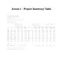
Produce Project Summary .......................................................................................................................................33
Export Results............................................................................................................................................................33
Manage HDM Output Files.....................................................................................................................................34
Edit Congestion Parameters...................................................................................................................................35
Manage Data Set Files.............................................................................................................................................35
Exiting the Program .................................................................................................................................................35
The Data Set Files.....................................................................................................................................................35
4
The HDM Manager Program
HDM Manager and HDM ........................................................................................................................................35
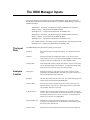
THE HDM M ANAGER INPUTS.......................................................................................................................................37
The Input Data...........................................................................................................................................................37
Analysis Control........................................................................................................................................................37
Road Characteristics................................................................................................................................................38
Required Vehicle Characteristics..........................................................................................................................45
Optional Vehicle Characteristics ..........................................................................................................................48
Operation Unit Costs................................................................................................................................................51
Definition of Strategies ............................................................................................................................................53
Paved Maintenance Policies ..................................................................................................................................53
Unpaved Maintenance Policies .............................................................................................................................57
Construction Policies...............................................................................................................................................59
Exogenous Cst-Bnf Policies ....................................................................................................................................60
ANNEX 1 - PROJECT SUMMARY TABLE................................................................................................................ i
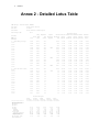
ANNEX 2 - DETAILED LOTUS TABLE......................................................................................................................II
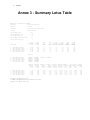
ANNEX 3 - SUMMARY LOTUS TABLE................................................................................................................... IV
The HDM Manager Program
Acknowledgments
The HDM Manager is a user-friendly shell environment for the Highway Design and Maintenance
Standards Model (HDM). The core HDM model was developed by Thawat Watanatada, Clell Harral,
William Paterson, Ashok Dhareshwar, Anil Bhandari, Koji Tsunokawa, Chris Hoban, and Rodrigo
Archondo-Callao.
The development of the HDM Manager software and documentation benefited from comments of many
individuals. Special thanks go to Chris Hoban, Gerard Liautaud, Cesar Queiroz, Roberto Armijo, Koji
Tsunokawa, and Raymond Charles, who motivated and guided its development.
5
6
The HDM Manager Program
The HDM Manager Program
Introducing
HDM
Manager
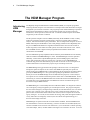
The Highway Design and Maintenance Standard Model (HDM) is a computer program for
analyzing the total transport costs of alternative road improvement and maintenance strategies
through life-cycle economic evaluation. The program provides detailed modeling of pavement
deterioration and maintenance effects, and calculates annual costs of road construction,
maintenance, vehicle operation, and travel time. Accidents and other impacts can be added
exogenously to the economic evaluation.
The first personal computer version of HDM, released by the World Bank in 1989, is widely
used in the evaluation of specific road proposals, national or regional road investments
analysis, and road maintenance policy assessment. The second personal computer version of
HDM, released by the World Bank in 1995 in this package, maintains total compatibility with
the previous HDM and addresses its significant limitation that it does not take account of
traffic congestion, and its effects on traffic speeds, travel times and road user costs. That is,
the 1995 HDM contains congestion analysis capabilities but maintains all the other
characteristics of 1989 HDM.
The use of HDM was greatly simplified with the release by the World Bank of a user-friendly
shell environment called HDM Manager in 1992. The HDM Manager stores the input data
efficiently, creates all the required HDM input files, runs the HDM program, collects the
results, and presents the results in a practical way. The first version of HDM Manager
evaluated only paved roads maintenance projects and the second version was improved to
evaluate maintenance and construction projects for paved and unpaved roads.
The HDM Manager being presented in this package is the third version. It is designed to
manage the inputs and outputs of the current 1995 HDM and optionally the inputs and
outputs of the previous HDM model. It also implements all the suggestions for improvements
given by the HDM Manager 2.1 users, specially regarding the presentation of the results.
While you can use the HDM Manager alone for demonstration purposes, it cannot analyze
new options or save new data without the presence of the 1995 or 1989 HDM models. On the
other hand, you could use the HDM models alone without the need for the HDM Manager. A
procedure that is not recommended for new HDM users because of cumbersome process
involved in using the HDM software.
The HDM Manager is a user-friendly shell environment for HDM. It is designed to evaluate a
set of road agency strategies applied to paved and unpaved roads. The program computes,
for each of the road agency strategies being evaluated, the road deterioration, the cost streams
(agency costs, road user costs, and total society costs), and the economic indicators (net
present value of net benefits and the internal rate of return) used to compare the set of road
agency strategies. As a result, the user obtains the strategy that yields the highest benefits to
society and if there is a budgetary constraint, the user obtains the optimal strategy as a
function of the budget constraint.
HDM Manager incorporates most but not all the features of HDM. The main HDM features
not included in this version are the following: i) division of roads to be evaluated (links) into
sections and subdivision of sections into subsections , ii) use of alternative vehicle operating
costs relationships, and iii) variable number of strategies to be evaluate in each run. To access
The HDM Manager Program
7
any of these features you would have to run the HDM model independently from the HDM
Manager following its instructions.
The HDM Manager 3.0 is compatible with the HDM Manager 2.1. That is, the HDM Manager
3.0 reads data files created with the HDM Manager 2.1 and both produce the same results if
the congestion analysis of the 1995 HDM model is disabled. The new features of HDM
Manager 3.0 are: a) manages 1995 HDM (new congestion inputs), b) new user impacts output
box, c) new cost-benefits policies option, d) new sensitivity analysis option, e) new economic
analysis indicators, f) ADT of cars can be higher than 9999, g) improved graphics, h) new
option for saving graphics, and i) use of extended memory if available.
The 1995 HDM system disk provided with this package contains the HDM Manager 3.0, the
The 1995
1995 HDM, the new EBM-HS Model, and three HDM case studies. To run these programs
HDM System you need a 80286 CPU or greater, DOS 3.1 or greater, 640 Kb of conventional memory, and a
disk space of 10 Mb. Also make sure that 30 or more files are defined in the CONFIG.SYS file.
Installing
1995 HDM
System
The steps needed to install the 1995 HDM system are the following:
Step 1
Insert the system disk in drive A:
Step 2
At the DOS prompt, enter the command:
A:INSTALL
The installation program expands the compressed files located on the system disk and copies
them to the following directories:
HDM
where the 1995 HDM program is located
HDM-MAN
where the HDM Manager 3.0 and the HDM Manager 3.0
Utilities are located
HDMCASE1
where the Gravel Road Case Study is located
HDMCASE2
where the Paved Road Case Study is located
HDMCASE3
where the Congestion Case Study is located
EBM-HS
where the EBM-HS model is located
If any of the directories does not exist, the installation program will create it. If you have a
previous version of the HDM, HDM Manager or EBM already installed on your computer,
note the following: a) The 1995 HDM does not interfere with the 1989 HDM (they are
composed of different and can be located on the same directory), b) If you have a previous
version of the HDM Manager in a directory called HDM-MAN, the install program will
overwrite it, and c) The EBM-HS program interferes with the previous EBM. Therefore, it is
installed in a directory called EBM-HS.
For instructions regarding the EBM-HS model, refer to the EBM-HS documentation. To
follow the HDM case studies, refer to their documentation. This document presents the HDM
Manager software and the input data.
8
The HDM Manager Program
Starting the
HDM
Manager
The HDM Manager is a program written for DOS that can be executed from within the
Windows 3.1 environment. This section and the following section present the procedures for
starting the HDM Manager using DOS commands. For instructions on how to install and
execute the HDM Manager on Windows 3.1, refer to the section tilted “Working with
Windows 3.1” that is given after the DOS instructions sections.
Using all the Defaults
To start the program using all the programs defaults, following the Steps below:
Step 1
Change to the HDM-MAN directory with the following DOS
command:
CD\HDM-MAN
Step 2
Run the HDM Manager with the command:
HDM-MAN
Storing Work Files in Other Directories
The default setup of the HDM Manager is to store the input files and output files in the HDMMAN directory (current directory). If you want to store all the input and output files in another
disk drive or directory (work area directory) to avoid mixing the program files with the data files
(procedure that is highly recommended), start the program as follow:
Step 1
Change to the HDM-MAN directory with the following DOS
command:
CD\HDM-MAN
Step 2
Run the HDM Manager with the command:
HDM-MAN
xxxxx
replace xxxxx with the work area directory. For example:
HDM-MAN
c:\hdmcase1\
Note that before starting the program in this manner, you should have created the work area
directory. For example, using the DOS command:
MD\HDMCASE1
Using Monochrome Monitors
HDM Manager detects if you have a color or monochrome board and sets the screen colors
accordingly. If you want to force HDM Manager to use the monochrome palette (for example
on portable computers), start the program as follows:
The HDM Manager Program
Step 1
9
Change to the HDM-MAN directory with the following DOS
command:
CD\HDM-MAN
Step 2
Run the HDM Manager with the command:
HDM-MAN
xxxxx
M
replace xxxxx with the work area directory. For example:
HDM-MAN
Working
with the
1989 HDM
Model
c:\hdmcase1\
M
This HDM Manager version is designed mainly to be used with the 1995 HDM. The 1995
HDM has an option designed to disable the congestion analysis and if the congestion
analysis is disabled, the model gives the same results as the 1989 HDM. Therefore, the use of
the previous HDM model is not necessary or recommended. In case you want to use the
HDM Manager with the previous HDM model, follow the steps below.
Install the 1989 HDM
Install 1989 HDM in a directory called HDM, following the instructions given by the
HDM-PC manual.
Install the 1995 HDM System
Install the 1995 HDM System following the steps described in the previous section.
Start the HDM Manager
To start the HDM Manager and access the 1989 HDM program, change to the HDMMAN directory with the following DOS command:
CD\HDM-MAN
and start the program with any of the following DOS commands:
a) To start the program with all the defaults:
HDM3-MAN
b) To store the data files in the directory xxxxx:
HDM3-MAN xxxxx
replace xxxxx with the work area directory
c) To store the data files in the directory xxxxx
and to display the monochrome palette:
HDM3-MAN xxxxx M.
10
The HDM Manager Program
replace xxxxx with the work area directory
The HDM Manager is a program written for DOS that can be executed from within the
Working
Windows 3.1 environment. To use the HDM Manager under Window, you first need to add
with
an icon to Windows that when activated will execute the HDM Manager. To install the HDM
Windows 3.1 Manager under Windows, follow the steps below.
Step 1
Select the File menu at the Windows Program Manager
Step 2
Select the New option at the File menu
Step 3
Select Program Item at the New Program Object dialog box
Step 4
Enter the following information at the Program Item Properties dialog
box
Description:
HDM Manager 3.0
Command Line:
HDM-MAN xxxx
Working Directory:
C:\HDM-MAN
Shortcut Key:
None
where xxxx should be replaced by the work area directory,
for example:
HDM-MAN c:\hdmcase1\
Note that when you are defining an icon for the HDM Manager, you specify the work area
directory that the HDM Manager will use to store the data files. Therefore, if you will be
working with different work area directories (for example working with the case studies
supplied in this package), you will need to add a separate icon for each work area directory
that you will be working. Each icon that you add should have on the Command Line, at the
Program Item Properties, the corresponding work area directory.
To start the HDM Manager under Windows, select the HDM Manager 3.0 icon. Windows
executes the HDM Manager and after you define the input data, the HDM Manager executes
the HDM program automatically and collects the results. Note that the HDM Manager is
being executed under Windows but it is not a Windows program. Therefore, you can not use
the mouse while working with the HDM Manager and you can not cut and paste information
to and from the Windows clipboard.
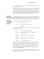
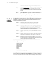
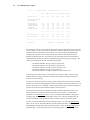
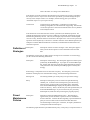
The Main
Menu
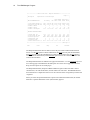
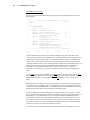
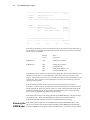
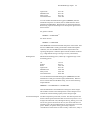
The main menu (shown below) shows you the basic structure of the program and gives you a
series of options (Analysis Control, Deterioration, etc.). At this type of menu, select an option
by using the cursor keys to highlight the option and pressing the Enter key or by pressing the
first letter of the option selected.
The HDM Manager Program
11
+--------- The Highway Design and Maintenance Standards Model Series ----------+
¦
Transportation, Water & Urban Development Department, The World Bank
¦
¦
HDM Manager, Version 3.0, 04/04/95
¦
¦
¦
¦ +---------------------+
+------------------+ ¦
¦ ¦ Analysis Control
+---+
+---¦ Deterioration
¦ ¦
¦ +---------------------+
¦
¦
+------------------+ ¦
¦
¦
¦
¦
¦ +---------------------+
¦
¦
+------------------+ ¦
¦ ¦Road Characteristics +---¦
+---------------+
+---¦
User Impacts
¦ ¦
¦ +---------------------+
¦
¦
¦
¦
+------------------+ ¦
¦
+---¦
HDM Model
¦---¦
¦
¦ +---------------------+
¦
¦
¦
¦
+------------------+ ¦
¦ ¦ Vehicle Fleet Data +---¦
+---------------+
+---¦
Cost Streams
¦ ¦
¦ +---------------------+
¦
¦
+------------------+ ¦
¦
¦
¦
¦
¦ +---------------------+
¦
¦
+------------------+ ¦
¦ ¦
Strategies
+---+
+---¦Economic Analysis ¦ ¦
¦ +---------------------+
+------------------+ ¦
¦
¦
¦
+-----------------+
+----------------+
¦
¦
¦ Other Options ¦
¦ Quit Program ¦
¦
¦
+-----------------+
+----------------+
¦
¦
¦
+------------------------------------------------------------------------------+
Learning the To do a basic life-cycle economic evaluation of a set of road agency strategies applied to a
paved or unpaved road, follow the Steps below:
Basics
Step 1
Define the Analysis Control. Enter the discount rate, the analysis
period, the calendar year of the initial year, and the currency to be
used.
Step 2
Define the Road Characteristics. Enter the road geometry, road
structure, road condition, environment, daily traffic, the traffic growth,
and congestion parameters.
Step 3
Define the Vehicle Fleet Data. Enter the vehicle fleet characteristics
and the vehicle operation unit costs.
Step 4
Define the Strategies. Enter the maintenance operations and
construction unit costs, define a data bank of possible road agency
maintenance and construction policies, and define the road agency
strategies to be evaluated.
Step 5
Execute the HDM Model. Run the HDM model from within the shell
environment. Note that after the HDM run is completed, the HDM
Manager collects the HDM results from the HDM output files.
Step 6
View the Deterioration. Examine the road deterioration behavior
(roughness progression, wide cracks progression, etc.) of each of the
road agency strategies being evaluated.
Step 7
View the User Impacts. Examine the user impacts (road user costs,
speeds, etc.) of each of the road agency strategies being evaluated.
Step 8
View the Cost Streams . Examine the financial and economic cost
streams (agency costs, road user costs, exogenous costs -benefits, and
12
The HDM Manager Program
total society costs) of the road agency strategies being evaluated.
Step 9
View the Economic Analysis . Examine the economic comparison of the
strategies being evaluated. The comparison is based on the net
present value of benefits (NPV) of each strategy in relation to a base
strategy.
Step 10
Explore Other Options. For example: i) perform sensitivity analysis, ii)
produce a project summary, iii) export the results to Lotus 1-2-2 or
Dbase, iv) view or print the original HDM output files, v) edit the
congestion setup tables, or vi) manage the data set files.
For each step described above, select the corresponding option at the main menu.
The Road
Agency
Strategies
The HDM Manager evaluates road agency strategies that are defined as sequence of actions
performed by a road agency during a defined analysis period to maintain and/or improve a
roadway. Some examples are given below:
Example 1
Maintain an unpaved road for twenty year by doing routine
maintenance, gravel resurfacing, and grading twice a year.
Example 2
Maintain an unpaved road for two years doing routine maintenance
and grading twice a year, and on the third year upgrade the road to a
paved standard to be follow in subsequent years (next seventeen
years) by routine maintenance, pothole patching and reseals activated
when the surface distress area is greater than 10 percent.
Example 3
Maintain a paved road by just doing routine maintenance for twenty
years.
Example 4
Maintain a paved road for twenty years by doing routine maintenance,
patching all the potholes and by doing overlays every eight years.
Example 5
Rehabilitate and widen the paved road in the first year to be follow in
the next nineteen years by routine maintenance and overlays activated
when the road roughness is greater than 4.5 IRI.
The actions performed by a road agency that can be included in the definition of a road
agency strategy are the following:
- Routine maintenance
- Grading a gravel road
- Gravel resurfacing
- Spot regravelling
- Pothole patching
- Reseals
- Overlays
- Reconstructions
- New Constructions or Upgradings
The timing of these actions is in control of the user. That is, the user defines if an action takes
place scheduled at a certain year or time interval, or if the action is activated in response to the
condition of the road. The HDM model and the HDM Manager do not generate strategies for
a given road. They perform a life-cycle economic evaluation of strategies defined by the user.
The HDM Manager Program
13
The next sections present the steps needed to setup the life-cycle economic evaluation and to
define the strategies to be evaluated.
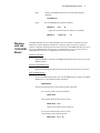
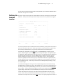
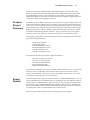
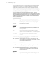
Defining the
Analysis
Control
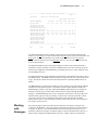
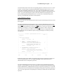
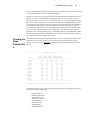
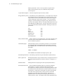
Select the Analysis Control option at the main menu to enter the control data to be used in the
HDM run. When you select this option, the Analysis Control screen (shown below) appears.
+----------------------------- Analysis Control -----------------------------+
¦
¦
¦ Description
Paving Gravel Road #1
¦
¦
¦
¦ Run Date
Day 08
Month 08
Year 94
¦
¦
¦
¦ Discount Rate (%)
12.0
¦
¦
¦
¦ Analysis Period (years)
20
¦
¦
¦
¦ Calendar Year of Initial Year
1995
¦
¦
¦
¦ Input Currency Name
Dollars
¦
¦
¦
¦ Output Currency Name
Dollars
¦
¦
¦
¦ Output Currency Conversion Multiplier
1.0000000
¦
¦
¦
¦
¦
¦
¦
¦
¦
+----------------------------------------------------------------------------+
Edit
Print
Keep
Get
Save/Exit
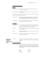
The screen presents the current information stored in the memory of the system and a menu of
options at the bottom of the screen. In this type of menu, you should select an option using
the arrow keys and the Enter key or by pressing the first letter of the selected option.
To modify any of the inputs, use the Edit option. The HDM Manager has three types of
inputs: i) required inputs, ii) optional inputs, and iii) lookup table inputs. The required inputs
are displayed in Black and should be entered by the user. The optional inputs are displayed in
Purple and in this case if the user wants the HDM model to estimate an optional input as a
function of other inputs, the user can leave the input empty (not zero). The lookup table
inputs are displayed in Brown and accept only a valid choice from a list of options. Press the
F10 key, when the cursor is at the input field, to display the list of valid options and select an
option with the Enter key. Note that you can not leave the lookup table inputs empty. They
are required inputs.
The information displayed on this type of screen (Blue background) is what will be used by
the HDM model to compute the results. The information on a screen is saved automatically in
the memory of the system by HDM Manager each time you exit the screen with the Save/Exit
option. That is, if you use the Save/Exit option to exit the screen and later you load the
program and go back to the screen, the information previously on the screen will be there.
You also have the option of storing in a file (data set file) the information currently on the
screen to create a library of information files that you can retrieve later. To store in a file the
information currently on the screen, use the Keep option. This option prompts for the name of
14
The HDM Manager Program
the data set file to store the information. Enter a file name of up to six characters or digits. The
HDM Manager will give a proper extension to the file.
To retrieve the information of a previously stored (using the Keep option) data set file, use
the Get option. This option lists the available data sets. Highlight the data set you want and
press the Enter key. The program will get the information from the data set file and present it
on the screen. Remember that the HDM model uses the current information displayed on the
screen (saved automatically with the Save/Exit option) to compute the results.
To print the current information, use the Print option and the program displays a list of valid
printers. Select your printer by highlighting the printer and pressing the Enter key.
To return to the main menu use the Save/Exit option. If you press the Escape key, the program
will return to the main menu but it will not save in the memory of the system the latest screen
changes. Note that in the HDM Manager at any moment you can press the Escape key to
cancel an operation or to go back to a previous menu.
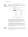
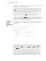
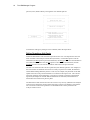
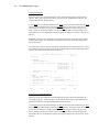
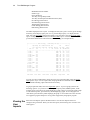
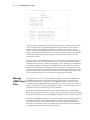
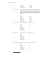
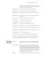
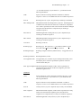
Select the Road Characteristics option at the main menu to enter the road information to be
Defining
used in the HDM run. When you select this option, the Road Characteristics screen (shown
Road
below) appears.
Characteris_
tics
+--------------------------- Road Characteristics ---------------------------+
¦
Page 1/3 ¦
¦ Description
Gravel Road #1 in North Region
¦
¦
¦
¦ Road Class (Paved/Unpaved)
U
¦
¦
¦
¦ GEOMETRY
¦
¦
Road Length (km)
100.0
Road Width (m)
6.0
¦
¦
One Shoulder Width (m)
0.4
Effective Number of Lanes
.
¦
¦
Rise & Fall (m/km)
40.0
Curvature (deg/km)
100.0
¦
¦
Superelevation (%)
0.0
¦
¦
¦
¦ ENVIRONMENT
¦
¦
Altitude (m)
500
Rainfall (m/month)
0.0300
¦
¦
¦
¦
¦
¦
¦
¦
¦
¦
¦
¦
¦
¦
¦
+--------------------------------------------------------------¦ Next Page +-+
Edit
Print
Keep
Get
Save/Exit
The Road Characteristics menu is similar to the Analysis Control menu. Use the Edit option to
edit the information, the Print option to print the information, the Keep option to store the
information into a data set file for future use, the Get option to retrieve a data set information,
and the Save/Exit option to save the current information and return to the main menu.
If you decide to store the current information (using the Keep option) in a data set file, you
can give to the road characteristics data set file name the same data set file name given to an
Analysis Control, Vehicle Fleet, Maintenance Unit Costs, Road Agency Policies, or a Road
Agency Strategies data set. That is, the HDM Manager program considers each set of
information (Analysis Control, Road Characteristics, Vehicle Fleet, Maintenance Unit Costs,
Policies and Strategies) to be independent of each other, assigning to each one a different
The HDM Manager Program
15
extension. Therefore, you could use the same data set file name for all the input sets.
The road characteristics data is divided into the following three screen pages: i) page 1
contains the road type, road geometry and environment data, ii) page 2 contains the road
structure and condition data, and iii) page 3 contains the current traffic, expected traffic growth
and congestion parameters. Note that the data requested on the second page changes as a
function of the road type (paved or unpaved road).
To move among the three pages use Next Page option or press the Page Up or Page Down
keys. When you use the Edit option, you edit the page being displayed. To edit another
page, you have to display the page and then use the Edit option again. When you use the
Print, Keep, and Get options, you are working with the data of all three pages. Therefore,
when you use the Keep option, you are storing the data of all three pages into a single data
set file and when you use the Print option, you are printing all the road characteristics.
Note that in page three if you don't want to include a particular vehicle type in the analysis,
you should enter 0 (zero) in the corresponding average daily traffic (ADT) field. Note also that
in page two for paved roads, you have the option of entering both the Structural Number and
the Benkelman Beam deflection or just either one of these variables, leaving the other blank.
This is an exceptional requirement for optional data (purple inputs).
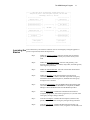
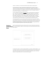
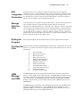
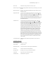
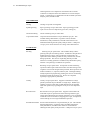
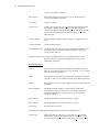
Select the Vehicle Fleet Data option at the main menu to enter the vehicle fleet characteristics
Defining
to be used in the HDM run. When you select this option, the Vehicle Fleet Data menu (shown
Vehicle Fleet below) appears.
Data
+------------------------------------------------------------------------------+
¦
¦
¦
+---------------------------------------------+ ¦
¦
¦
¦ ¦
¦
¦
¦ ¦
¦
¦
¦ ¦
¦
¦
+---------------------------+
¦ ¦
¦
¦
¦
Required Parameters
¦
¦ ¦
¦
¦
+---------------------------+
¦ ¦
¦
¦
¦ ¦
¦
¦
¦ ¦
¦
¦
+---------------------------+
¦ ¦
¦ +---------------------+
¦
¦
Optional Parameters
¦
¦ ¦
¦ ¦ Vehicle Fleet Data ¦----¦
+---------------------------+
¦ ¦
¦ +---------------------+
¦
¦ ¦
¦
¦
¦ ¦
¦
¦
¦ ¦
¦
¦
¦ ¦
¦
¦
¦ ¦
¦
¦
¦ ¦
¦
¦
¦ ¦
¦
¦
Exit
¦ ¦
¦
+---------------------------------------------+ ¦
+------------------------------------------------------------------------------+
You have three options: i) enter the required parameters, ii) enter the optional parameters, or iii)
exit the menu. Select an option using the arrow keys and the Enter key or by pressing the first
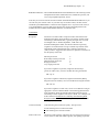
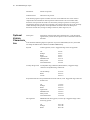
letter of the selected option. When you select the Required Parameters option , the Vehicle
Fleet Data - Required Parameters screen (shown below) appears.
16
The HDM Manager Program
+----------------- Vehicle Fleet Data - Required Parameters -----------------+
¦
Page 1/2 ¦
¦ Description
Required Data for North Region
¦
¦
¦
¦
Light Medium Heavy Artic. ¦
¦ BASIC CHARACTERISTICS
Car Pickup
Bus Truck Truck Truck Truck ¦
¦
¦
¦ Gross Vehicle Weight (t) 1.200 1.800 10.900 5.600 11.300 20.800 27.000 ¦
¦ ESAl Factor per Veh.(E4) 0.000 0.010 0.500 0.100 1.000 3.000 5.000 ¦
¦ Number of Axles
2
2
2
2
2
3
5 ¦
¦ Number of Tires
4
4
6
6
6
10
18 ¦
¦ Number of Passengers
3.00
3.00 40.00
0.00
0.00
0.00
0.00 ¦
¦
¦
¦ VEHICLE UTILIZATION DATA
¦
¦
¦
¦ Service Life (yr)
10.0
8.0
8.0
8.0
8.0
8.0
8.0 ¦
¦ Hours Driven per Year
450
1300
2000
1300
2100
2000
1900 ¦
¦ Km Driven per Year
18000 30000 80000 50000 65000 67500 80000 ¦
¦ Depreciation Code
2
2
2
2
2
2
2 ¦
¦ Utilization Code
1
3
3
3
3
3
3 ¦
¦ Annual Interest Rate (%) 12.00 12.00 12.00 12.00 12.00 12.00 12.00 ¦
+--------------------------------------------------------------¦ Next Page +-+
Edit
Print
Keep
Get
Save/Exit
The Required Parameters menu is similar to the Analysis Control and Road Characteristics
menus. Use the Edit option to edit the information, the Print option to print the information,
the Keep option to store the information into a data set file for future use, the Get option to
retrieve a data set information, and the Save/Exit option to save the current information and
return to the main menu.
The Required Parameters are defined in two pages of information. Use the Next Page option to
move among pages. Remember that the Edit option acts on the current page while the Print,
Keep, and Get options act on all the pages.
The Required Parameters (all inputs in Black and Brown) option collects the basic vehicle
characteristics, the vehicle utilization, and the vehicle unit costs data. The HDM model uses
this information to compute the road user cost as a function of the road geometry and the road
roughness.
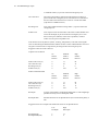
When you select the Optional Parameters option at the Vehicle Fleet Data menu, the Vehicle
Fleet Data - Optional Parameters screen (shown below) appears.
The HDM Manager Program
17
+----------------- Vehicle Fleet Data - Optional Parameters -----------------+
¦
Page 1/2 ¦
¦ Description
Optional Data for Norht Region
¦
¦
¦
¦
Light Medium Heavy Artic. ¦
¦ VEHICLE PARAMETERS
Car Pickup
Bus Truck Truck Truck Truck ¦
¦
¦
¦ Payload (Tons)
0.20
0.40
3.50
2.80
7.60 12.80 22.00 ¦
¦ Aerodynamic Drag Coeff.
.
.
.
.
.
.
.
¦
¦ Projected Frontal Area
.
.
.
.
.
.
.
¦
¦ Driving Power (Metric HP)
.
.
.
.
.
.
. ¦
¦ Braking Power (Metric HP)
.
.
.
.
.
.
. ¦
¦ Paved Desired Spd (km/h)
98.30 94.90 93.40 81.60 88.80 88.80 84.10 ¦
¦ Unpaved Desired Sp (km/h) 82.20 76.30 69.40 71.90 72.10 72.10 49.60 ¦
¦ Energy Efficiency Factor
0.85
0.95
0.95
0.95
0.95
0.95
0.95 ¦
¦ Hourly Utilization Ratio
.
.
.
.
.
.
.
¦
¦ Calibrated Eng Spd (rpm)
.
.
.
.
.
.
. ¦
¦ Weibull Shape Parameter
.
.
.
.
.
.
.
¦
¦ Max Avg Rect Vel (mm/s)
.
.
.
.
.
.
.
¦
¦ Width Parameter for Spd
.
.
.
.
.
.
.
¦
¦ Fuel Adjustment Factor
.
.
.
.
.
.
.
¦
+--------------------------------------------------------------¦ Next Page +-+
Edit
Print
Keep
Get
Save/Exit
The Optional Parameters menu is similar to the Analysis Control and Road Characteristics
menus. Use the Edit option to edit the information, the Print option to print the information, the
Keep option to store the information into a data set file for future use, the Get option to
retrieve a data set information, and the Save/Exit option to save the current information and
return to the main menu.
The Optional Parameters option (all inputs in Purple) is used to enter the data required to
calibrate the vehicle operating costs model. Remember that if you want to change any of the
default values supplied by the HDM model, you should enter the new values, otherwise leave
the fields blank (not zero).
For detailed information on the information requested at the Vehicle Fleet Data option, refer to
the HDM manuals. The HDM manuals describe each input item, the units used, and the valid
range. This option contains the vehicle fleet characteristics required by HDM (series D in
HDM).
The HDM Manager program adopts the Brazil vehicle operating costs relationships of HDM
and defines seven types of vehicles. The number of vehicle types defined is fixed by the
HDM Manager program. Therefore, while the full HDM program allows you to change the
number of vehicle types and their names, these cannot be changed through the HDM
Manager. The HDM Manager allows you to change the characteristics of each of the seven
defined vehicle types and if in your analysis you don't want to include a particular vehicle
type, enter 0 (zero) in the corresponding average daily traffic (ADT) field at the Road
Characteristics option. Note also that the currency used to enter the unit costs is defined in
the Analysis Control screen.
Working
with
Strategies
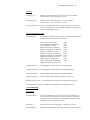
Select the Strategies option at the main menu to define the road agency strategies to be
evaluated in the HDM run. This option displays the Strategies Menu screen (shown below).
You have six options: i) enter the maintenance and construction operations unit costs, ii)
define the road agency strategies, iii) define a library of paved road maintenance policies, iv)
define a library of unpaved road maintenance policies, v) define a library of construction
18
The HDM Manager Program
policies, and vi) define a library of exogenous costs-benefits policies.
+---------------------------------------------+
¦
¦
¦
+------------------------------+
¦
¦
¦
Operations Unit Costs
¦
¦
¦
+------------------------------+
¦
¦
¦
¦
¦
¦
+------------------------------+
¦
¦
¦
Definition of Strategies
¦
¦
¦
+------------------------------+
¦
¦
¦
¦
¦
¦
+- Policies Data Bank ----------------+
¦
¦
¦
Paved Maintenance Policies
¦
¦
+---------------------+
¦
¦
Unpaved Maintenance Policies
¦
¦
¦
Strategies
¦----¦
¦
Construction Policies
¦
¦
+---------------------+
¦
¦
Exogenous Cst-Bnf Policies
¦
¦
¦
+-------------------------------------+
¦
¦
¦
¦
Exit
¦
+---------------------------------------------+
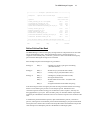
To define the road agency strategies to be evaluated, follow the steps below:
Define Operations Unit Costs
Define the maintenance and construction operations unit costs. The Operations Unit Costs
menu is similar to the Analysis Control menu (see below). Use the Edit option to edit the
information, the Print option to print the information, the Keep option to store the information
into a data set file for future use, the Get option to retrieve a data set information, and the
Save/Exit option to save the current information and return to the previous menu.
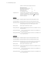
The unit costs entered are the costs for a particular (user defined) operation. For example, in
the screen below: the financial unit cost for an overlay is equal to 10.81 $/km, the thickness
and the material being defined by the user. This cost, for example, may be based on a 40 mm
asphalt concrete overlay, but these details are not shown in the input screen. The cost for a
particular operation can be adjusted by a cost factor to consider variations on the defined
operation (for example to consider different thicknesses or materials) in the definition of
maintenance and construction policies phase.
The maintenance and construction unit costs can be in any currency (defined in the Analysis
Control screen) and will be used by all the road agency policies to be defined. Note that the
unit cost for the construction operation is in thousands of the currency defined in the
Analysis Control screen.
The HDM Manager Program
19
+-------------------- Strategies - Operations Unit Costs --------------------+
¦
¦
¦ Description
Operation Costs for North Region
¦
¦
¦
¦
Financial Economic ¦
¦ Operation
Unit Cost Unit Cost ¦
¦
¦
¦ Grading (Currency per km of road graded)
100.0
85.0
¦
¦ Spot Regraveling (Currency per cu m)
10.00
8.50
¦
¦ Gravel Resurfacing (Currency per cu m)
20.00
17.00
¦
¦ Unpaved Routine Maintenance (Currency per km per yr)
500
425
¦
¦
¦
¦ Patching (Currency per sq m)
10.00
8.50
¦
¦ Resealing (Currency per sq m)
2.70
2.30
¦
¦ Overlay (Currency per sq m)
10.81
9.19
¦
¦ Reconstruction (Currency per sq m)
40.00
34.00
¦
¦ Paved Routine Maintenance (Currency per km per yr)
1500
1275
¦
¦
¦
¦ Construction (Thousands currency per km)
100.0
85.0
¦
¦
¦
¦ Note: The input currency is defined in the Analysis Control Data
¦
+----------------------------------------------------------------------------+
Edit
Print
Keep
Get
Save/Exit
Define Policies Data Bank
The HDM Manager evaluates road agency strategies that are composed of one or more than
one paved maintenance policy, unpaved maintenance policy, construction policy, or
exogenous costs -benefits policy. Therefore, you have to create a data bank of road agency
policies before defining the strategies to be evaluated.
Some examples of policies and strategies are given below::
Strategy X:
Policy 1
- Grading every 90 days, plus gravel resurfacing
(from 1995 to 2014)
Strategy Y:
Policy 1
Policy 2
- Reseals every 4 years (from 1995 to 2004)
- Overlays every 8 years (from 2005 to 2011)
Strategy Z:
Policy 1
Policy 2
Policy 3
- Grading every 90 days (from 1995 to 1996)
- Paving the road (in 1997)
- Reseals when area of cracks > 15% (from 1998
to 2014)
- Exogenous benefits activated after the paving
Policy 4
Note that strategies are the road agency alternatives being evaluated and that each strategy
defines a set of future agency actions over the analysis period. Maintenance and
construction policies within a strategy are not alternatives, but a sequence, with only one
being applicable in a given year. Note also that a policy can include a number of operations
which may be scheduled at a fixed time interval or activated in response to the condition of the
road.
You define the paved maintenance policies, unpaved maintenance policies, construction
policies, and exogenous costs-benefits policies that should belong to your policies data bank .
These policies are stored in data set files with unique file names and should have unique and
clear descriptions to identify the policies at the Definition of Strategies phase.
20
The HDM Manager Program
Paved Maintenance Policies
When you select the Paved Maintenance Policies option at the Strategies menu, the screen
below appears.
+------------------ Data Bank - Paved Maintenance Policies ------------------+
¦
Page 1/3 ¦
¦ Description
¦
¦
¦
¦ Yes/No
¦
¦
Y
ROUTINE MAINTENANCE
¦
¦
Features:
Cost factor
1.00
¦
¦
¦
¦
N
PATCHING
(Scheduled or Responsive) R
¦
¦
Scheduled:
Area to be patched (m2/km/y)
0.0
¦
¦
Responsive: Percent of pothole area to be patched
0.0
¦
¦
Maximum applicable area (m2/km/y)
.
¦
¦
Features:
Cost factor
1.00
¦
¦
Last applicable year
¦
¦
Maximum applicable roughness (IRI)
.
¦
¦
¦
¦
N
RESEALING
(Scheduled or Responsive) R
¦
¦
Scheduled:
Resealing interval (y)
0
¦
¦
Responsive: Maximum allowable total damaged area (%)
0.0
¦
¦
Minimum applicable resealing interval (y)
¦
¦
Maximum applicable resealing interval (y)
¦
+--------------------------------------------------------------¦ Next Page +-+
Edit
Print
Save
Retrieve
Exit
The Paved Maintenance Policies menu is different from the Analysis Control menu or the
other previous input data menus described so far. To indicate that, the screen background is
Green while at the previous input data screens the backgrounds are Blue. On the Blue input
screens, after you select the Save/Exit option, the program saves and retains in memory the
information displayed on the screen. This information is then used by the HDM program. The
Green input screens are managing a Data Bank of policies stored on files. Therefore, the
information is not retained in memory when you select the Exit option. To save the
information related to a policy, you have to explicitly use the Save option and supply a file
name.
Use the Edit option to edit the information, the Print option to print the information, the Save
option to save the information in a file, the Retrieve option to retrieve previously saved
information for editing or viewing purposes, and the Exit option to return to the previous
menu.
Remember that in this Step you are not deciding which policies to include in the strategies to
be evaluated. You are managing a series of road agency policies stored in files that could or
could not be used by the HDM model. You define the policies to be included in each strategy
and the timing of these policies in the Definition of Strategies phase.
The Paved Maintenance Policies information is composed of three screen "pages". In these
pages, you define the maintenance operations included in the policy and the characteristics of
the operations. A paved maintenance policy is composed of Routine Maintenance and if
wanted other maintenance operations (Patching, Reseal, Overlay or Reconstruction). Each
maintenance operation can be scheduled at a certain time interval or activated in response to
the condition of the road. Note that the Routine Maintenance operation is always included
and that you can have more than one operation in a policy.
To show that a certain operation should be included on the policy being defined, enter a "Y"
The HDM Manager Program
21
at the left column of the screen at the corresponding operation. Otherwise, enter "N" or leave
it blank. To select the type of operation (Scheduled or Responsive) place an "R" or "S" at
right of the "Scheduled or Responsive" line. If you select the Scheduled option, enter the
information at the Scheduled line (lines) and disregard the information on the Responsive line
(lines). If you select the Responsive option, enter the information at the Responsive line
(lines), and disregard the Scheduled line (lines). In both cases, Scheduled or Responsive
options, you should define the Features of the operation.
Unpaved Maintenance Policies
When you select the Unpaved Maintenance Policies option at the Strategies menu, the screen
below appears.
The Unpaved Maintenance Policies menu is equal to the Paved Maintenance Policies menu.
Use the Edit option to edit the information, the Print option to print the information, the Save
option to save the information in a file, the Retrieve option to retrieve previously saved
information for editing or viewing purposes, and the Exit option to return to the previous
menu. When you use the Save option, you are requested to enter a six digit/character file
name and when you use the Retrieve option, the program displays a list of the previously
saved policies.
+----------------- Data Bank - Unpaved Maintenance Policies -----------------+
¦
Page 1/2 ¦
¦ Description
¦
¦
¦
¦ Yes/No
¦
¦
Y
ROUTINE MAINTENANCE
¦
¦
Features:
Cost factor
1.00
¦
¦
¦
¦
N
GRADING
(Scheduled or Responsive)
R
¦
¦
Scheduled:
Time interval between gradings (d)
0
¦
¦
Responsive: Traffic interval between grading (vet)
0
¦
¦
Minimum applicable time interval (d)
¦
¦
Maximum applicable time interval (d)
¦
¦
Features:
Cost factor
1.00
¦
¦
¦
¦
N
SPOT REGRAVELLING (Scheduled or Responsive) R
¦
¦
Scheduled:
Gravel volume (m3/km/y)
0.0
¦
¦
Responsive: Percent annual material loss replaced (%)
0
¦
¦
Maximum applicable gravel volume (m3/km/y)
.
¦
¦
Features:
Cost factor
1.00
¦
¦
¦
+--------------------------------------------------------------¦ Next Page +-+
Edit
Print
Save
Retrieve
Exit
Remember that the inputs in Black are required inputs, the inputs in Purple are optional (you
can leave them blank, not zero, to be estimated by HDM), and the inputs in Brown are
obtained from a list of valid options (press F10).
The Unpaved Maintenance Policies structure is similar to the Paved Maintenance Policies
structure. The only difference is the type of operations included (Grading, Spot Regravelling,
and Gravel Resurfacing). Remember that you select an operations by placing a "Y" at the left
of the operation line, you decide between a Scheduled or Responsive operation by placing an
"R" or "S" at the right of the corresponding line, and that you should enter the features of the
operation.
22
The HDM Manager Program
Construction Policies
When you select the Construction Policies option at the Strategy menu, the screen below
appears. The Construction Policies menu is equal to the Paved Maintenance Policies and
Unpaved Maintenance Policies menus.
Use the Edit option to edit the information, the Print option to print the information, the Save
option to save the information in a file, the Retrieve option to retrieve previously saved
information for editing or viewing purposes, and the Exit option to return to the previous
menu. When you use the Save option, you are requested to enter a six digit/character file
name and when you use the Retrieve option, the program displays a list of previously saved
policies.
Remember that each policy should have a unique file name and a unique description. While
defining the strategies, you will identify the policies that are part of a strategy through the
policy description.
The Construction Policies option requests the characteristics of a construction policy. That is,
the construction duration and costs, the new road characteristics, and an optional generated
traffic to be activated at the end of the construction.
+-------------------- Data Bank - Construction Policies ---------------------+
¦
Page 1/3 ¦
¦ Description
¦
¦
¦
¦ CONSTRUCTION
¦
¦
Construction Duration (y)
1
¦
¦
Annual Cost Stream (% of total cost):
Construction Year 1
0.0
¦
¦
Construction Year 2
0.0
¦
¦
Construction Year 3
0.0
¦
¦
Construction Year 4
0.0
¦
¦
Construction Year 5
0.0
¦
¦
Salvage Value (% of total cost)
0.0
¦
¦
Cost Factor
1.00
¦
¦
¦
¦ GEOMETRY
¦
¦
Road Class (Paved/Unpaved)
P
¦
¦
Road Length (km)
1.0
Road Width (m)
2.5
¦
¦
One Shoulder Width (m) 0.0
Effective Number of Lanes
.
¦
¦
Rise & Fall (m/km)
0.0
Curvature (deg/km)
0.0
¦
¦
Superelevation (%)
.
¦
¦
¦
+--------------------------------------------------------------¦ Next Page +-+
Edit
Print
Save
Retrieve
Exit
Exogenous Costs-Benefits Policies
When you select the Exogenous Costs-Benefits Policies option at the Strategy menu, the
screen below appears. The Exogenous Costs-Benefits Policies menu is equal to the Paved
Maintenance Policies and Unpaved Maintenance Policies menus.
Use the Edit option to edit the information, the Print option to print the information, the Save
option to save the information in a file, the Retrieve option to retrieve previously saved
information for editing or viewing purposes, and the Exit option to return to the previous
menu. When you use the Save option, you are requested to enter a six digit/character file
name and when you use the Retrieve option, the program displays a list of previously saved
policies.
The HDM Manager Program
23
+------------------ Data Bank - Exogenous Cst-Bnf Policies ------------------+
¦
¦
¦ Description
¦
¦
¦
¦ Year
Costs (+) or Benefits (-)
Year
Costs (+) or Benefits (-)
¦
¦
(Million Currency)
(Million Currency)
¦
¦
1
0.00
14
0.00
¦
¦
2
0.00
15
0.00
¦
¦
3
0.00
16
0.00
¦
¦
4
0.00
17
0.00
¦
¦
5
0.00
18
0.00
¦
¦
6
0.00
19
0.00
¦
¦
7
0.00
20
0.00
¦
¦
8
0.00
21
0.00
¦
¦
9
0.00
22
0.00
¦
¦ 10
0.00
23
0.00
¦
¦ 11
0.00
24
0.00
¦
¦ 12
0.00
25
0.00
¦
¦ 13
0.00
¦
¦
¦
¦ Note: The input currency is defined in the Analysis Control Data
¦
+----------------------------------------------------------------------------+
Edit
Print
Save
Retrieve
Exit
The Exogenous Costs-Benefits Policies option defines a stream of extra costs or benefits to be
activated when the policy is activated in the definition of strategies phase. The years in these
policies are relative years. That is, year one represents the year the policy is activated, year
two the following year and so on. Note that to assign extra benefits to a strategy you should
enter negative values and to assign extra costs you should enter positive values.
Define Strategies
The HDM Manager evaluates and compares five road agency strategies at a time. Each
strategy is composed of one or more than one road agency policy that is valid for a certain
period. The program always analyzes five strategies. Therefore, you always have to define
five strategies even if you are interested in the results of only one or two strategies. You
could use the other strategies to do some sensitivity analysis. Of the five strategies being
defined, the first strategy is the base strategy for comparison (the do minimum case). That is,
the program computes the net benefits of the remaining strategies is relation to the first
strategy.
When you select the Define Strategies option, the screen below appears. The Definition of
Strategies menu is similar to the Analysis Control menu. Use the Edit option to edit the
information, the Print option to print the information, the Keep option to store the information
into a data set file for future use, the Get option to retrieve a data set information, and the
Save/Exit option to save the current information and return to the previous menu.
To define the strategies enter the description of the set of five strategies and for each strategy
define the policies (or policy) that compose the strategy. For each strategy, define at least the
following information:
- The description of the strategy
- The starting year of the first maintenance policy
- The description of the first maintenance policy
24
The HDM Manager Program
+------------------ Strategies - Definition of Strategies -------------------+
¦
Page 1/2 ¦
¦ Description
Paving Gravel Road #1 / Run C
¦
¦
¦
¦ STRATEGY 1:
Grade Every 120 Days
¦
¦
Start in Year: 1995 Policy: Grading (120 days), Regravelling (Unp:G120_R)¦
¦
(
)¦
¦
(
)¦
¦
(
)¦
¦
¦
¦ STRATEGY 2:
Pave the Road in 1995
¦
¦
Start in Year: 1995 Policy: Wait for Paving
(Unp:WAIT )¦
¦
1995
Paving Gravel Road #1
(Con:PAV_01)¦
¦
1996
Reseal (12mm,20%), Patching
(Pav:SST_20)¦
¦
(
)¦
¦
¦
¦
¦
¦
¦
¦
¦
¦ Note: Strategy 1 is the base strategy for the economic analysis
¦
¦
¦
+--------------------------------------------------------------¦ Next Page +-+
Edit
Print
Keep
Get
Save/Exit
Each strategy should have at least one maintenance policy and the first policy should start at
the calendar year of the beginning of the analysis period. Each strategy can have a maximum
of four policies. For example:
Starting
in year
Policy
Description
STRATEGY 1
1995
Grading every 90 days
STRATEGY 2
1995
1996
1997
2005
Grading every 90 days
Paving the road
Reseal when damage > 15%
Overlays when IRI > 4.5
A maintenance policy will be active from the starting year up to the end of the analysis period,
unless a new policy starts. If a new maintenance policy starts, the previous policy will be
stopped. The construction policies are active from the starting year and for the duration of the
construction. The exogenous costs-benefits policies are active from the starting year to the
end of the analysis period.
Enter the starting calendar year for each policy and on the right side enter the policy
description. To enter a policy description, press the F10 key while the cursor is positioned at
the description field. When you press the F10 key, at a policy description field, the program
lists all the available policies (in your policies data bank stored in your work area directory).
Select a policy by highlighting it and pressing the enter key.
Note that the first strategy is the strategy defined by the HDM Manager as the base strategy
(do minimum case). That is, the HDM Manager computes the economic benefits of
implementing the other strategies in relation to implementing the first strategy.
Running the
HDM Model
After defining all the input data, run the HDM model using the HDM Model option. This
option creates all the input data files required by HDM, runs the HDM model automatically,
and after the HDM run is completed, collects the HDM results. Note that you need 3.5 Mb of
empty hard disk to store the temporary files created by the HDM model. These temporary files
The HDM Manager Program
25
empty hard disk to store the temporary files created by the HDM model. These temporary files
are erased automatically when you exit the HDM Manager.
If there is an input data or system error detected by the HDM model, the HDM model will not
generate the results. The HDM Manager program indicates this fact by giving you a error
message. If there is an input data error, you should locate it by viewing the output HDM scan
files. Use the Other Options option at the main menu and select “Manage HDM Output Files”.
View the SCAN 1 file to locate errors on the Analysis Control and Road Characteristics Data.
View the SCAN 2 file to locate errors on the Vehicle Fleet Data and Road Agency Policies.
View the SCAN 3 file to locate errors on the Road Agency Strategies and the structure of the
run and to obtain a summary table of errors and warnings. View the SCAN 4 file to locate
execution errors. After locating the errors, you should fix them and run the HDM model again.
Note that if the HDM model is not installed on your hard disk, the HDM Manager presents an
error message and doesn't compute the results.
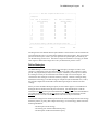
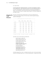
Viewing the
Road
Deterioratio
n
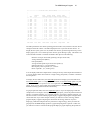
Select the Deterioration option at the main menu to view the road deterioration under the five
standards being evaluated. When you select this option, the periodic operations table
appears and if you select the Next Table option, the following roughness deterioration table
appears.
+--------------------------- Roughness (IRI m/km) ---------------------------+
¦
¦
¦
¦
¦
First
Second
Third
Fourth
Fifth
¦
¦
Year
Strategy Strategy Strategy Strategy Strategy
¦
¦-- ---- -------------------- -------- -------- -------- --------------------¦
¦ 1 1995 ¦
11.2
12.4
12.4
12.4
12.4
¦
¦ 2 1996 ¦
12.0
3.2
13.9
13.9
13.9
¦
¦ 3 1997 ¦
12.2
3.3
3.2
14.3
14.3
¦
¦ 4 1998 ¦
12.4
3.4
3.3
3.2
14.5
¦
¦ 5 1999 ¦
10.8
3.4
3.4
3.3
3.2
¦
¦ 6 2000 ¦
11.0
3.5
3.4
3.4
3.3
¦
¦ 7 2001 ¦
11.2
3.6
3.5
3.4
3.4
¦
¦ 8 2002 ¦
11.4
3.7
3.6
3.5
3.5
¦
¦ 9 2003 ¦
11.6
3.8
3.7
3.6
3.5
¦
¦10 2004 ¦
11.4
3.9
3.8
3.7
3.6
¦
¦11 2005 ¦
11.9
4.0
3.9
3.8
3.7
¦
¦12 2006 ¦
12.1
4.1
4.0
3.9
3.8
¦
¦13 2007 ¦
12.2
4.2
4.1
4.0
3.9
¦
¦14 2008 ¦
11.9
4.3
4.2
4.1
4.0
¦
¦15 2009 ¦
12.6
4.4
4.3
4.2
4.1
¦
+----------------------------------------------------------------------------+
Next Table
Prev. Table
Select Table
Graph Table
Output Table
Exit
The Roughness table presents the roughness progression for all five strategies and it is only
one of the following available tables:
Capital Operations
Roughness (IRI m/km)
All Cracks Area (%)
Wide Cracks Area (%)
Area Ravelled (%)
Pothole Area (%)
Rut Depth (mm)
SD Rut Depth (mm)
26
The HDM Manager Program
Modified Structural Number
Surface Type
Gravel Thickness
Two-Way Average Daily Traffic
Two-Way Annual Equivalent Standard Axles ('000)
First Strategy Deterioration
Second Strategy Deterioration
Third Strategy Deterioration
Fourth Strategy Deterioration
Fifth Strategy Deterioration
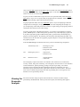
The tables display the first 15 years. To display the next years (years 16 to 25), press the Page
Down key, and to display again years 1 to 15, press the Page Up key. To display the next
table, select the Next Table option and to display a previous table, select the Previous Table
option. To display a particular table, use the Select Table option. Note that the last five tables
present all the deterioration characteristics for each strategy (see example below).
+------------------ First Strategy - Grade Every 120 Days ------------------+
¦
¦
¦
Oper Rough All Wide Rave Potho Rut
Gra
Annual ¦
¦
atio ness Crck Crck lled
les Dpth Mod Sur
vel 2-Way
2-Way ¦
¦
Year ns
IRI
%
%
%
%
mm
SN face
mm
ADT ESA 000 ¦
¦-- ---- ----- ----- ----- ---- ---- ----- ---- ---- ---- ---- ----- --------¦
¦ 1 1995 ¦
11.2
GRAV 122
200
23.8 ¦
¦ 2 1996 ¦
12.0
GRAV
93
207
24.5 ¦
¦ 3 1997 ¦
12.2
GRAV
64
215
25.3 ¦
¦ 4 1998 ¦RESU 12.4
GRAV 184
223
26.0 ¦
¦ 5 1999 ¦
10.8
GRAV 154
231
26.8 ¦
¦ 6 2000 ¦
11.0
GRAV 122
239
27.6 ¦
¦ 7 2001 ¦
11.2
GRAV
90
248
28.4 ¦
¦ 8 2002 ¦
11.4
GRAV
57
258
29.3 ¦
¦ 9 2003 ¦RESU 11.6
GRAV 174
267
30.2 ¦
¦10 2004 ¦
11.4
GRAV 140
277
31.1 ¦
¦11 2005 ¦
11.9
GRAV 105
287
32.0 ¦
¦12 2006 ¦
12.1
GRAV
69
298
33.0 ¦
¦13 2007 ¦RESU 12.2
GRAV 183
309
34.0 ¦
¦14 2008 ¦
11.9
GRAV 145
321
35.0 ¦
¦15 2009 ¦
12.6
GRAV 107
333
36.0 ¦
+----------------------------------------------------------------------------+
Next Table
Prev. Table
Select Table
Graph Table
Output Table
Exit
To print, save into an ASCII file or export to Lotus 1-2-3 a particular table, select the Output
Table option. If you save or export a table, the program asks for a filename. Enter a legitimate
DOS filename including a path and extension if necessary.
To graph a particular table, select the Graph Table option. To print a graph you have the
following options: a) to produce a screen dump to an Epson printer, IBM Proprinter, or HP
LaserJet printer, press the F7 key while displaying a graph, and b) to print a high quality graph
in a HP LaserJet printer, press the F9 key while displaying a graph. To save the graph in a
.PCX format, press the F4 key while displaying the graph. You can then retrieve the .PCX file
into a graphics program and print it on any printer supported by the graphics program.
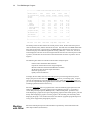
Viewing the
User
Impacts
Select the User Impacts option at the main menu to view the user impacts for the five
strategies being evaluated. When you select this option, the following unit road user costs
table appears.
The HDM Manager Program
27
+--------------------- Road User Costs (Dollars/veh-km) ---------------------+
¦
¦
¦
¦
¦
Vehicle
First
Second
Third
Fourth
Fifth
¦
¦
Year
Type
Strategy Strategy Strategy Strategy Strategy
¦
¦--- ---- ---------------- --------- -------- -------- -------- -------------¦
¦ 1 1995
Car
¦
0.25
0.27
0.27
0.27
0.27
¦
¦ 2 1996
Car
¦
0.26
0.17
0.29
0.29
0.29
¦
¦ 3 1997
Car
¦
0.27
0.17
0.17
0.29
0.29
¦
¦ 4 1998
Car
¦
0.27
0.17
0.17
0.17
0.30
¦
¦ 5 1999
Car
¦
0.25
0.17
0.17
0.17
0.17
¦
¦ 6 2000
Car
¦
0.25
0.17
0.17
0.17
0.17
¦
¦ 7 2001
Car
¦
0.25
0.18
0.17
0.17
0.17
¦
¦ 8 2002
Car
¦
0.26
0.18
0.18
0.17
0.17
¦
¦ 9 2003
Car
¦
0.26
0.18
0.18
0.18
0.17
¦
¦ 10 2004
Car
¦
0.26
0.18
0.18
0.18
0.18
¦
¦ 11 2005
Car
¦
0.26
0.18
0.18
0.18
0.18
¦
¦ 12 2006
Car
¦
0.27
0.18
0.18
0.18
0.18
¦
¦ 13 2007
Car
¦
0.27
0.18
0.18
0.18
0.18
¦
¦ 14 2008
Car
¦
0.26
0.18
0.18
0.18
0.18
¦
¦ 15 2009
Car
¦
0.27
0.18
0.18
0.18
0.18
¦
+----------------------------------------------------------------------------+
Next Table
Prev. Table
Select Table
Graph Table
Output Table
Exit
The table presents the unit vehicle operating plus travel time costs (road user costs) for all five
strategies and for all vehicles. The tables display the first 15 years for the first vehicle. To
display the next years (years 16 to 25) and the next vehicles, press the Page Down key, and to
display again years 1 to 15 and the previous vehicles, press the Page Up key. This table is one
of several tables available. The tables available at this option are the following:
Road user costs per vehicle-km (operating costs plus travel time)
Average annual speed (km/hr)
Free speed (km/hr)
Average annual speeds as percent of free speeds (%)
Speeds in periods 1, 2, 3, 4 and 5 (km/hr)
Flow-capacity ratios in periods 1, 2, 3, 4 and 5
Flows in periods 1, 2, 3, 4 and 5 (pc/hr)
You can display tables that compare the five strategies for any of the outputs described above
or you can display tables that contain for a single strategy the speeds, F-C Ratios or the flows
for each period.
To display the next table select, the Next Table option and to display a previous table select,
the Previous Table option. To display a particular table, use the Select Table option. To print,
save into an ASCII file or export to Lotus 1-2-3 a particular table, select the Output Table
option. If you save or export a table, the program asks for a filename. Enter a legitimate DOS
filename including a path and extension if necessary.
To graph a particular table, select the Graph Table option. If you are displaying a table that
compares the five strategies, when you select the graph option, you will be presented with two
options: (i) compare strategies, or (ii) compare vehicles. If you select compare strategies, you
will have to select a vehicle and the program displays a graph comparing the strategies for the
vehicle selected. If you select compare vehicles, you will have to select a strategy and the
program displays a graph comparing the vehicles for the strategy selected. If you are
displaying a table that compares the five periods for a single strategy, when you select the
graph option, the HDM Manager produces a graph comparing the five periods. In this case,
you will have to select a vehicle and the program displays a graph comparing the periods for
28
The HDM Manager Program
the vehicle selected.
To print a graph you have the following options: a) to produce a screen dump to an Epson
printer, IBM Proprinter, or HP LaserJet printer, press the F7 key while displaying a graph, and
b) to print a high quality graph in a HP LaserJet printer, press the F9 key while displaying a
graph. To save the graph in a .PCX format, press the F4 key while displaying the graph. You
can then retrieve the .PCX file into a graphics program and print it on any printer supported by
the graphics program.
Viewing the
Cost
Streams
Select the Cost Streams option at the main menu to view the cost streams for the five
strategies being evaluated. When you select this option, the following financial agency
capital costs table appears.
+------------- Financial Agency Capital Costs (Million Dollars) -------------+
¦
¦
¦
¦
¦
First
Second
Third
Fourth
Fifth
¦
¦
Year
Strategy Strategy Strategy Strategy Strategy
¦
¦-- ---- ------------------- --------- --------- --------- ------------------¦
¦ 1 1995 ¦
0.000
10.000
0.000
0.000
0.000
¦
¦ 2 1996 ¦
0.000
0.000
10.000
0.000
0.000
¦
¦ 3 1997 ¦
0.000
0.000
0.000
10.000
0.000
¦
¦ 4 1998 ¦
1.920
0.000
0.000
0.000
10.000
¦
¦ 5 1999 ¦
0.000
0.000
0.000
0.000
0.000
¦
¦ 6 2000 ¦
0.000
0.000
0.000
0.000
0.000
¦
¦ 7 2001 ¦
0.000
0.000
0.000
0.000
0.000
¦
¦ 8 2002 ¦
0.000
0.000
0.000
0.000
0.000
¦
¦ 9 2003 ¦
1.920
0.000
0.000
0.000
0.000
¦
¦10 2004 ¦
0.000
0.000
0.000
0.000
0.000
¦
¦11 2005 ¦
0.000
0.000
0.000
0.000
0.000
¦
¦12 2006 ¦
0.000
0.000
0.000
0.000
0.000
¦
¦13 2007 ¦
1.920
0.000
0.000
0.000
0.000
¦
¦14 2008 ¦
0.000
1.998
0.000
0.000
0.000
¦
¦15 2009 ¦
0.000
0.000
1.998
0.000
0.000
¦
+----------------------------------------------------------------------------+
Next Table
Prev. Table
Select Table
Graph Table
Output Table
Exit
This table is only one of the following available tables:
Financial Agency Capital Costs
Financial Agency Recurrent Costs
Economic Agency Capital Costs
Economic Agency Recurrent Costs
Economic Road User Costs
Economic Travel Time Costs
Economic Exogenous Costs-Benefits
Economic Total Society Costs
Net Economic Benefits
First Strategy Economic Costs
Second Strategy Economic Costs
Third Strategy Economic Costs
Fourth Strategy Economic Costs
Fifth Strategy Economic Costs
The tables display the first 15 years. To display the next years (years 16 to 25), press the Page
Down key, and to display again years 1 to 15, press the Page Up key. To display the next table
The HDM Manager Program
29
select, the Next Table option and to display a previous table select the Previous Table option.
To display a particular table, use the Select Table option. Note that the last five tables present
all the cost streams for each strategy.
To print, save into an ASCII file or export to Lotus 1-2-3 a particular table, select the Output
Table option. If you save or export a table, the program asks for a filename. Enter a legitimate
DOS filename including a path and extension if necessary.
To graph a particular table, select the Graph Table option. If you are displaying a table that
compares the five strategies, the program displays a bar chart comparing the strategies. If
you are displaying a table that presents the costs for a single strategy, the program produces a
stacked bar chart with the costs of the strategy.
To print a graph you have the following options: a) to produce a screen dump to an Epson
printer, IBM Proprinter, or HP LaserJet printer, press the F7 key while displaying a graph, and
b) to print a high quality graph in a HP LaserJet printer, press the F9 key while displaying a
graph. To save the graph in a .PCX format, press the F4 key while displaying the graph. You
can then retrieve the .PCX file into a graphics program and print it on any printer supported by
the graphics program.
Note that HDM Manager divides the total society costs into the following components:
Total Society Costs =
Road Agency Costs
+ Road User Costs
+ Exogenous Costs-Benefits
and
Road Agency Costs =
Capital Costs
+ Recurrent Costs
and
Road User Costs =
Vehicle Operation
+ Travel Time
The road agency capital costs are the costs related to new construction, reconstruction,
overlays, reseals, and gravel resurfacing. The road agency recurrent costs are costs related to
routine maintenance, pothole patching, gradings, and sport regravelling. The vehicle
operation costs are related to the fuel consumption, lubricants consumption, tire wear,
maintenance parts, maintenance labor, depreciation, interest lost, and crew time. The travel
time costs are related to the passenger time and cargo holding time. The exogenous costsbenefits costs are specified by the user.
Viewing the
Economic
Analysis
Select the Economic Analysis option at the main menu to view the economic analysis
performed by the HDM model. When you select this option, the following table appears.
30
The HDM Manager Program
+---------------- Present Values and Internal Rate of Return ----------------+
¦
¦
¦-Present Values at ¦ First
Second
Third
Fourth
Fifth
¦
¦ 12.0% Discount Rate¦ Strategy
Strategy
Strategy
Strategy
Strategy ¦
¦ (Million
¦---------- ---------- ---------- ---------- ---------- ¦
¦ Dollars)
¦
¦
¦
¦
¦
¦ Society
¦
37.20
32.85
33.21
33.61
34.04 ¦
¦ Agency
¦
3.08
9.79
8.77
7.87
7.06 ¦
¦
Capital
¦
2.51
8.79
7.84
6.99
6.23 ¦
¦
Recurrent
¦
0.57
1.00
0.94
0.88
0.84 ¦
¦ Road Users
¦
34.13
23.06
24.43
25.74
26.98 ¦
¦
Vehicle Operation¦
24.53
16.28
17.30
18.28
19.20 ¦
¦
Travel Time
¦
9.60
6.78
7.13
7.46
7.77 ¦
¦ Exogenous Cst-Bnf ¦
0.00
0.00
0.00
0.00
0.00 ¦
¦
¦
¦
¦ Net Present Value ¦
0.00
4.35
4.00
3.59
3.16 ¦
¦ (Net Benefits)
¦
¦
¦
¦
¦
¦-Rate of Return (%) ¦
NA
18.9
19.2
19.3
19.3 ¦
¦
¦
¦
+----------------------------------------------------------------------------+
Next Table
Prev. Table
Select Table
Graph Table
Output Table
Exit
The table presents the discounted cost streams present values, the discounted net present
value of benefits (NPV), and the internal rate of return. Note that if the core HDM model finds
many rates of return for a given strategy, the HDM Manager computes the various rates of
return and dis plays one of them along with the warning “(MANY)”. In this case, the rate of
return displayed is the first rate of return higher than the discount rate if the net present value
is positive, and the first rate of return lower than the discount rate if the net present value is
negative.
The following five tables are available in the Economic Analysis option:
Present Values and Internal Rate of Return
Equivalent Annual Values and Average Roughness
Benefit Cost Ratios and Incremental Benefit Cost Ratios
Net Present Value per Initial Capital Investment
Financial Agency Costs
Quality of Service Indicators
To display the next table, select the Next Table option or press the Page Down key and to
display the previous table select the Previous Table option or press the PgUp key. To print,
save into an ASCII file or export the table to Lotus 1-2-3, select the Output Table option. If
you save or export the table, the program asks for a filename. Enter a legitimate DOS filename
including a path and extension if necessary.
Select the Graph Table option to graph the table. There are different graph options for each
table being displayed. To print a graph you have the following options: a) to produce a
screen dump to an Epson printer, IBM Proprinter, or HP LaserJet printer, press the F7 key
while displaying a graph, and b) to print a high quality graph in a HP LaserJet printer, press the
F9 key while displaying a graph. To save the graph in a .PCX format, press the F4 key while
displaying the graph. You can then retrieve the .PCX file into a graphics program and print it
on any printer supported by the graphics program.
Working
with Other
Select the Other Options option at the main menu to perform any of the tasks listed in the
Other Options menu (shown below).
The HDM Manager Program
31
with Other
Options
+----------------------------------------------------------------------------+
¦
¦
¦ +--------------------------------+
+-------------------------------+ ¦
¦ ¦ 1 Perform Sensitivity Analysis ¦
¦ 4 Manage HDM Output Files
¦ ¦
¦ +--------------------------------+
+-------------------------------+ ¦
¦
¦
¦ +--------------------------------+
+-------------------------------+ ¦
¦ ¦ 2 Produce Project Summary
¦
¦ 5 Edit Congestion Tables
¦ ¦
¦ +--------------------------------+
+-------------------------------+ ¦
¦
¦
¦ +--------------------------------+
+-------------------------------+ ¦
¦ ¦ 3 Export Results
¦
¦ 6 Manage Data Set Files
¦ ¦
¦ +--------------------------------+
+-------------------------------+ ¦
¦
¦
¦
¦
¦
Exit
¦
¦
¦
+----------------------------------------------------------------------------+
¦
+-----------------+
¦ Other Options ¦
+-----------------+
The other options are the following:
1) Perform Sensitivity Analysis. This option allows you to perform a sensitivity
analysis of the economic evaluation of a given strategy.
2) Produce Project Summary. This option allows you to produce a one page summary
report of the results of the economic evaluation of a given strategy.
3) Export Results. This option allows you to export the results to Lotus 1-2-3, Dbase
and EBM formats.
4) Manage HDM Outputs. This option allows you to view, print, and keep the output
files created by the HDM model.
5) Edit Congestion Tables. This option allows you to modify the congestion setup
tables after the congestion calibration process.
6) Manage Data Set Files. This option allows you to delete and copy the Data Set
files used during an HDM run.
Perform
Sensitivity
Analysis
This option allows you to perform a sensitivity analysis of the economic evaluation of a given
strategy by increasing or decreasing the net cost streams and by changing the discount rate
used to compute the net present value of benefits (NPV). When you select this option, the
program requests the selection of a strategy to be evaluated and after you select a strategy, a
screen similar to the one shown below appears:
32
The HDM Manager Program
+---------------- Second Strategy - Pave the Road in 1995 -----------------+
¦
¦
¦
Study 1 Study 2 Study 3 Study 4 Study 5 Study 6¦
¦
¦
¦ Discount Rate (%)
12.00
12.00
12.00
12.00
12.00
12.00 ¦
¦
¦
¦ Multiplicative Factors
¦
¦ for Net Benefits
¦
¦
¦
¦ Agency Capital
1.00
1.20
1.00
1.20
1.30
1.40 ¦
¦ Agency Recurrent
1.00
1.20
1.00
1.20
1.30
1.40 ¦
¦ Vehicle Operation
1.00
1.00
0.80
0.80
0.70
0.60 ¦
¦ Travel Time
1.00
1.00
0.80
0.80
0.70
0.60 ¦
¦ Exogenous Cst-Bnf
1.00
1.00
0.80
0.80
0.70
0.60 ¦
¦
¦
¦
------- ------- ------- ------- ------- ------- ¦
¦
¦
¦ Net Present Value
4.36
3.02
2.14
0.80
-0.98
-2.75 ¦
¦
¦
¦ Rate of Return (%)
18.90
16.10
15.50
13.10
10.70
8.40 ¦
¦
¦
+----------------------------------------------------------------------------+
Edit Factors
Graph Table
Output Table
Exit
The sensitivity analysis screen shows the net present value and the internal rate of return for
six case studies. For each case study, the discount rate and the multiplicative factors for net
benefits used in the calculations are also shown. For a given strategy, the HDM model
computes the net present value and the internal rate of return from a stream of total net
benefits and the discount rate. The stream of total net benefits represents the benefits of
implementing the strategy in relation to implementing the base strategy (first strategy). The
stream of total benefits is the sum of the following streams:
- Net benefits related to savings in agency capital costs
- Net benefits related to saving in agency recurrent costs
- Net benefits related to savings in vehicle operation costs
- Net benefits related to savings in travel time costs
- Net benefits related to savings in exogenous costs-benefits costs
Note that the net benefits streams contain positive and negative values. Positive values
indicate benefits (savings) and negative values indicate negative benefits (increases) in
relation to the base strategy.
For each case study, the sensitivity analysis option computes the net present value and the
internal rate of return by multiplying the streams of net benefits by user-specified factors and
the given discount rate. For example, a vehicle operation factor of 0.8 represents taking in to
account only 80 percent of the benefits related to vehicle operation.
The sensitivity analysis option computes the results with the multiplicative factors and
discount rate that are currently stored on the memory of the system. To change these
parameters, use the Edit Factors option. Once you change these parameters, the program
computes again the results and presents them on the screen. The new parameters will be
saved on the memory of the system and will be used the next time you use this option.
To print, save into an ASCII file or export the table to Lotus 1-2-3, select the Output Table
option. If you save or export the table, the program asks for a filename. Enter a legitimate
DOS filename including a path and extension if necessary. Select the Graph Table option to
graph the table. To print a graph you have the following options: a) to produce a screen
The HDM Manager Program
33
dump to an Epson printer, IBM Proprinter, or HP LaserJet printer, press the F7 key while
displaying a graph, and b) to print a high quality graph in a HP LaserJet printer, press the F9
key while displaying a graph. To save the graph in a .PCX format, press the F4 key while
displaying the graph. You can then retrieve the .PCX file into a graphics program and print it
on any printer supported by the graphics program.
Produce
Project
Summary
The produce project summary option allows you to produce a one page summary report of the
results of the economic evaluation of a given strategy. Select the Project Summary option to
view, print, or export a summary report for your selected project (see Annex 1). Your selected
project should be one of the four strategies being analyzed (second strategy to fifth strategy).
Remember that the first strategy is the base strategy (without project case) used to compute
the benefits of implementing the other strategies. After you select the project, the program
asks if you want to view, print, save (ASCII) or export (Lotus 1-2-3) the summary report.
The summary report presents for the without project case (first strategy) and for the selected
project the following information:
- Roughness Progression
- Average Daily Traffic
- Periodic Maintenance Actions
- Economic Road Agency Costs
- Economic Road User Costs
- Economic Total Society Costs
It also presents the following economic comparison indicators:
- Decrease in Agency Costs Stream
- Decrease in User Costs Stream
- Net Economic Benefits Stream
- Project Net Present Value
- Project Internal Rate of Return
The economic road agency costs are the sum of the capital and recurrent costs. The economic
road user costs are, in this table, the sum of the vehicle operation, travel time costs and
exogenous costs -benefits. Note that if you export the summary report to Lotus 1-2-3, it will
also present the financial agency costs of the project.
Export
Results
This option allows you to export the results to Lotus 1-2-3, Dbase and EBM formats. You can
create a Detailed Lotus 1-2-3 Table (see Annex 2), a Summary Lotus 1-2-3 Table (see Annex 3),
a Dbase Table, or an EBM input file. When you select a Lotus 1-2-3 table , the program asks
for a filename. Enter a legitimate DOS filename including a path if necessary. Note that you
don't have to include the .WK1 extension in the filename. The Lotus 1-2-3 tables can be used
to prepare plots or charts, or perform further analysis of the results.
When you select the Dbase Results Table the following input screen appears:
34
The HDM Manager Program
+---+-¦ Create Dbase Results Table +---------------------------------------+-+
¦
¦
¦ ¦
¦ +¦
FILE TO
¦ ¦
¦ ¦¦
BE CREATED
¦ ¦
¦ +¦
¦ ¦
¦
¦ DOS filename
: \MANAGER3\GRAV.DBF
¦ ¦
¦ +¦ Road code
: GRAV
¦ ¦
¦ ¦¦ Strategy 1 code : GRAD
¦ ¦
¦ +¦ Strategy 2 code : PAVI
¦ ¦
¦
¦ Strategy 3 code : PAVI
¦ ¦
¦ +¦ Strategy 4 code : PAVI
¦ ¦
¦ ¦¦ Strategy 5 code : PAVI
¦ ¦
¦ +¦
¦ ¦
¦
¦ -------------------------------------------------------------------- ¦ ¦
¦
¦
¦ ¦
¦
¦ Road Name : Gravel Road 1 in North Region
¦ ¦
¦
¦ Strategy 1 : Grading every 90 days + Regrav.
¦ ¦
+---¦ Strategy 2 : Paving in 1993 + Reseal at 20%
¦-+
¦ Strategy 3 : Paving in 1994 + Reseal at 20%
¦
¦ Strategy 4 : Paving in 1995 + Reseal at 20%
¦
¦ Strategy 5 : Paving in 1996 + Reseal at 20%
¦
¦
¦
+----------------------------------------------------------------------+
You should enter the DOS filename, including a path if necessary, and the road and strategy
codes. The Dbase tables created from different runs can be merged to store the results of
different roads into a single Dbase table for further analysis at a network level. For this
purpose, when creating the Dbase Results Table, you should give to each road and to each
strategy a four character identification code. The default road code is the first four characters
of the road description and the default strategy codes are the first four characters of the
strategies descriptions.
When you select to create an EBM Input File, the program presents an input screen similar to
the Dbase Results Table input screen (shown above). You should enter the DOS filename,
including a path if necessary, and the road and strategy codes. Although it is not mandatory,
an extension of .EBM is recommended. Each EBM file to be created needs a four character
identification code for the road and the strategies being evaluated. The default road code is
the first four characters of the road description and the default strategy codes are the first four
characters of the strategies descriptions. Note that if you enter a filename that already exists,
the program asks if you want to overwrite the file or append to the existing file.
Manage
HDM Output
Files
This option allows you to view, print, and keep the output files created by the HDM model.
The HDM model produces 10 output files that contain all the inputs, error messages and
warnings, and all the results. Select the "View the HDM Output Files" option to view the
output files created by HDM model or any text (ASCII) file. When you select this option and
the file to view, the file you selected is displayed on the screen. Use the arrow keys to move
through the file and press the ESC key to return to the menu.
Select the "Print the HDM Output Files" option to print the output files created by HDM
model. When you select this option, you have to select the file you want to print and a printer
from a list of available printers. Note that the HDM output files contain 132 characters per line.
Select the "Keep HDM Output Files" option to store the HDM output files. Each time you run
the HDM Manager, the previous HDM output files created by the previous HDM run are
overwritten. Therefore, use this option to make a copy of these output files for future use
before they are overwritten. When you select the file you want to keep, the program asks for
the filename (include path and extension) to copy the file.
The HDM Manager Program
35
Edit
Congestion
Parameters
This option allows you to modify the congestion lookup tables after the congestion
calibration process. Use the “Edit Road Types” option to edit the road types lookup tables.
You have the option of editing road types, adding road types and deleting road types. Use
the “Edit Road Uses” option to edit the road uses lookup tables. You have the option of
editing road uses, adding road uses and deleting road uses.
Manage
Data Set
Files
This option allows you to delete and copy the Data Set files. Select the "Delete a Data Set"
option to delete a data set of a particular input module (Analysis Control, Road
Characteristics, Vehicle Fleet Data, etc.). Select the "Copy a Data Set" option to copy a data
set of a particular input module (Analysis Control, Road Characteristics, Vehicle Fleet Data,
etc.) to a different drive or directory. Select the "Copy all Data Set" option to copy all data
sets to a different drive or directory. When you select the “Delete” or “Copy” options, the
program enters into a loop that allows you to delete or copy many Data Sets quicker. To exit
the loop, select the “Return to Main Menu” option.
Exiting the
Program
Select the Quit Program option at the main menu to exit the program and return to DOS.
The Data Set All Data Set files created by the HDM Manager are Dbase files. The filenames start with the
character "_" and the second character indicates the type of data the file contains. We have
Files
the following:
_A
_B
_C
_D
_E
_F
_G
_H
_I
_J
_K
_L
HDM
Manager
and HDM
Run Control Data
Reserved for Future Use
Road Characteristics
Reserved for Future Use
Required Vehicle Parameters
Optional Vehicle Parameters
Maintenance Unit Costs
Definition of Standards
Paved Maintenance Policies
Unpaved Maintenance Policies
Construction Policies
Exogenous Cst-Bnf Policies
The HDM Model reads a series of input files (ASCII text files) and after it computes the
results, it creates another series of output text files. The HDM Manager program stores the
input data and the results in Dbase files. Therefore, the HDM input files you created with
your word processor or with the HDM Input Data Facility are not compatible with HDM
Manager. That means that you cannot import the data stored in HDM input files into the
HDM Manager.
The HDM Manager creates all the required HDM input files before it runs the HDM model.
These files are named HDMDATA.*. That is, HDMDATA.RUN, HDMDATA.AAA,
HDMDATA.BBB, etc. You can view and modify these files with a word processor or the
HDM Input Data Facility to run the HDM model directly.
The HDM Manager Inputs
This section describes the input data used by the HDM Manager. Refer to the following
World Bank publications for additional information regarding the HDM Manager inputs and
HDM relationships:
Watanatada, T. and others. The Highway Design and Maintenance Standards
Model, Volume 1, Description of the HDM-III Model.
Washington, D.C.: Transportation Department, World Bank, 1987.
Watanatada, T. and others. The Highway Design and Maintenance Standards
Model, Volume 2, User’s Manual for the HDM-III Model.
Washington, D.C.: Transportation Department, World Bank, 1987.
Chris Hoban and others. Economic Analysis of Road Projects with Congested Traffic.
Washington, D.C.: Infrastructure Department, World Bank, 1995.
The Input
Data
Analysis
Control
The HDM Manager has the following three types of inputs:
Required
The required inputs are displayed in Black. You should enter these
inputs.
Optional
The optional inputs are displayed in Purple. You can leave these
inputs blank (not zero), if you want the HDM Model to estimate these
inputs as a function of other inputs or collect default values.
Lookup Table
The lookup table inputs are displayed in Brown. These inputs accept
only a valid choice from a list of options. To display the lookup table,
press the F10 key, when the cursor is at the input field.
Description
Description of the run. This description appears in all the reports
produced by the HDM Manager and when you use the Get option to
retrieve information stored in data files.
Run Date
Calendar day, month and year of the run. This information appears on
all the reports produced by the HDM Manager.
Discount Rate
Discount rate used to compute the present value of the costs and
benefits streams, in percent. For developing countries, the discount
rate generally adopted is 12 percent.
Analysis Period
Number of years to be included in the life-cycle economic evaluation,
in years. That is, the time over which benefits and costs are compared.
You options are between 10, 15, 20, or 25 years. An analysis period
between 15 to 20 years is recommended.
Initial Calendar Year
Calendar year of first year in the analysis period. Note that all the
strategies to be defined for the run should have a maintenance policy
that starts in this calendar year.
Input Currency
Name of the currency being used to enter the unit vehicle operation,
38 The HDM Manager Inputs
maintenance , construction, and exogenous costs. The program can
accept any currency, but you should use a currency that will fit on the
input fields. If a currency does not fit, you can use a multiplier of the
currency (for example: millions of pesos).
Output Currency
Name of the currency to be use to present the results. If the results do
not fit in the output fields, select a different output currency. Note
that the name you enter here will appear in all the reports produced by
the HDM Manager.
Conversion Multiplier Factor to convert from input currency to output currency. The output
currency will be the input currency multiplied by the output currency
conversion multiplier.
Description
Road
Characteris_
tics
Road Type
Description of the road. This description appears in all the reports
produced by the HDM Manager and when you use the Get option to
retrieve information stored in data files. If you plan to a create the
EBM input file, the first four characters of the description should be
the road code (project code) needed by the EBM program to identify
the road.
Code to identify the road type. Enter P to specify a paved road or U to
specify an unpaved road. Note that the second page of the road
characteristics inputs changes as a function of the road type.
PAVED AND UNPAVED ROADS
GEOMETRY
Road Length
Road length, in kilometers. Note that the minimum length possible is 1
kilometer.
Road Width
Carriageway width, in meters.
One Shoulder Width
Width of one shoulder, in meters.
Effective Number
of Lanes
Effective number of lanes. If value is not specified, the program
estimates the effective number of lanes as a function of the road
width. Estimated values:
1.0 if width < 4.5 m
1.5 if 4.5 m < width < 6.0 m
2.0 if 6.5 m < width < 8.0 m
3.0 if 8.0 m < width < 11.0 m
4.0 if 11.0 > width
Rise Plus Fall
Aggregate measure of the vertical gradient of a road in, m/km. It is
defined as the sum of the absolute values, in meters, of all ascents and
all descents along a road, divided by the length of the road in
kilometers. Suggested values:
Flat terrain
Level terrain
Rolling terrain
0
10
20
The HDM Manager Inputs
Hilly terrain
Mountainous terrain
Curvature
50
80
Aggregate of the horizontal curvature of the roadway, in degrees/km.
It is defined as the sum of the absolute values of angular deviations (in
degrees) of successive tangent lines of the road alignment when
traveling in one direction, divided by the road length in km. Suggested
values:
Flat terrain
Level terrain
Rolling terrain
Hilly terrain
Mountainous terrain
Superelevation
39
0
50
150
300
500
Average superelevation is defined as the weighted average of the
superelevations of the curvy sections of the road, the weights being
the proportion of the lengths of curvy sections. (dimensionless). The
superelevation of a curvy section is the vertical distance between the
heights of the inner and outer edges of the road divided by the road
width. If value is not specified, the program estimates the
superelevation as a function of the road curvature. Note that this
value has no significant effect on the results.
ENVIRONMENT
Altitude
Mean elevation of the road section above the mean sea level, in
meters. Note that this value has no significant effect on the results.
Rainfall
Mean monthly precipitation, in m/month. Suggested values:
Arid environment
Semiarid environment
Subhumid environment
Humid environment
0.002
0.020
0.080
0.150
PAVED ROADS
SURFACE
Surface Type
Code that indicates the surface type. The seven surface type codes
are:
1 for surface treatment (ST) roads
2 for asphalt Concrete (AC) roads
3 for slurry on surface treatment (SSST) roads
4 for reseal on surface treatment (RSST) roads
5 for reseal on asphalt concrete (RSAC) roads
6 for open graded cold mix on surface treatment (OCMS) roads
7 for asphalt overlay or slurry seal on asphalt concrete, and asphalt
overlay on surface treatment (OVSA) roads
Two of the surface types, surface treatment and asphalt concrete,
apply to original, new or reconstructed pavements. The other types
40 The HDM Manager Inputs
define surfaces after a full-width maintenance treatment or
rehabilitation of an existing pavement.
New Layers Thickness Total thickness of the most recent surfacing layers (or layer), in mm.
Old Layers Thickness Total thickness of previous, underlying surfacing layers (or layer), in
mm. If a road was constructed 20 years ago and an overlay was
applied 5 years ago, the layers (or layer) of the construction period are
the “old” layers and the layers (or layer) of the overlay are the “new”
layers. Note that when a pavement surface is applied to a road it can
be applied in one single layer or in more than one layer.
BASE/SUBGRADE
Base Type
Code that indicates the base type. The three base type codes are:
1 for granular bases
2 for cement stabilized bases
3 bituminous bases
Subgrade CBR
The California Bearing Ratio of the subgrade, in percent. It is
determined at the equilibrium in situ conditions of moisture content
and density. Suggested values:
Poor roadbed soil
Fair roadbed soil
Good roadbed soil
2
5
10
Base Layers Thickness Thickness of base layers in the original pavement, in mm. Note that
this input is only required if the base is cement stabilized.
Resilient Modulus
Resilient modulus of soil cement, in Gpa. Note that this input is only
required if the base is cement stabilized.
STRENGTH
Structural Number
Measure of pavement strength that summarize the complex
interactions between material types and stiffness. The structural
number (AASHTO) is defined as a linear combination of layer strength
coefficients and thicknesses of the individual layers above the
subgrade. Typical values:
Surface treatment (12 mm) road
Surface treatment (25 mm) road
Asphalt Concrete (5 cm) road
Asphalt Concrete (8 cm) road
Asphalt Concrete (10 cm) road
Asphalt Concrete (15 cm) road
1.0
1.5
2.0
3.0
4.0
5.5
Note that the roads described above are classified only by the surface
thickness with the assumption of having proper base layers. In the
computation of the structural number, the thicknesses of all layers
above the subgrade should be taken into account.
The HDM Manager Inputs
41
Benkelman Deflection The mean Benkelman Beam rebound deflection of the surfacing in both
wheelpaths under 80 kN standard axle load, 520 kPa tire pressure, and
30 C average asphalt temperature, in mm.
Note that you can enter both the structural number and the Benkelman Bean deflection or you
can enter only one of these values. If you enter only one of these values, the other will be
estimated by the HDM Model as a function of the supplied value. If you have both values, it
is recommended that you enter both values because the current relationship between the
modified structural number and Benkelman deflection is somewhat weak.
CONDITION
Roughness
Deviation of a surface from a true planar surface with characteristic
dimensions that affect vehicle dynamics, ride quality, dynamic loads
and drainage (ASTM E-867-82A) - typically in ranges of 0.1 to 100 m
wavelengths and 1 to 100 mm amplitudes , in IRI. IRI is the
International Roughness Index, the reference measure expressing
roughness as a dimensionless average rectified slope statistic of the
longitudinal profile and defined in Sayer, Gillespie, and Paterson
(1987), in m/km. Suggested values based on a qualitative evaluation of
the ride quality of the road:
Smooth paved road
Reasonably smooth paved road
Medium rough paved road
Rough paved road
Very rough paved road
2
4
6
8
10
If you have roughness in QI units (roughness measured by a
quarter-car index scale), convert it into IRI units using the formula:
IRI = QI / 13
If you have roughness in BI units (roughness measured by Bump
Integrator trailer at 32 km/h), convert it into IRI units using the formula:
IRI = BI / 715
If you have roughness in other units, convert it into IRI units using an
appropriate conversion method. Refer to the following publication for
more information about the International Roughness Index and its
relationship to other roughness units. Sayers, M.W., T.D. Gillespie and
W.D.O. Paterson. Guidelines for Conducting and Calibrating Road
Roughness Measurements. Technical Paper No. 46, The World Bank.
Washington, DC, 1986.
Construction Fault
Code indicating the construction quality. The options are:
0 if the surfacing has not construction faults
1 if the surfacing has construction faults
Wide Cracks Area
Total area of wide cracking, comprising the area of the interconnected
or line cracks of 3 mm crack width or greater, with spalling (equivalent
42 The HDM Manager Inputs
to AASHTO Class 4), in percent of the total carriageway area.
All Cracks Area
Total area of all cracking, comprising wide and narrow cracking, in
percent of the total carriageway area. Note that narrow cracks area is
the area of the interconnected or line cracks of 1-3 mm crack width
(equivalent to AASHTO Class 2).
Ravelling Area
Area of loss of material from wearing surface., in percent of the total
carriageway area.
Pothole Area
Area of open cavities in road surface with at lest 150 mm diameter and
at least 25 mm depth, in percent of the total carriageway area. Note
that a road in poor condition, with a series of potholes, will have
around 1.0 (one) percent of pothole area.
Note that the area of any distress (cracks, ravelling, and potholes) is the sum of rectangular
areas circumscribing the manifest distress and that for line cracks a width dimension of 0.5 m is
assigned. The distresses are expressed as percentage of the total carriageway area.
Suggested values for surface distress:
Asphalt Concrete Roads
Wide Cracks Area (%)
All Cracks Area (%)
Ravelling Area (%)
Pothole Area (%)
No
Surface
Distress
Medium
Surface
Distress
High
Surface
Distress
0
0
0
0
15
25
0
0.01
60
75
0
1.0
No
Surface
Distress
Medium
Surface
Distress
High
Surface
Distress
0
0
0
0
15
25
50
0.01
60
75
15
1.0
Surface Treatment Roads
Wide Cracks Area (%)
All Cracks Area (%)
Ravelling Area (%)
Pothole Area (%)
Rut Depth
Average of the measures of maximum depth under a 1.2 m straightedge
placed transversely across a wheelpath, in mm.
Rut Depth STD
Standard deviation of rut depth measures (across both wheel paths), in
mm.
Suggested values for rut depth and standard deviation of rut depth measures:
Rut Depth (mm)
Rut Depth STD (mm)
Low
Rut Depth
High
Rut Depth
5
2
15
6
The HDM Manager Inputs
43
HISTORY
Surfacing Age
Number of years elapsed since latest reseal, overlay, pavement
reconstruction, or new construction, in years.
Construction Age
Number of years elapsed since latest overlay, pavement
reconstruction, or new construction, in years.
Previous Wide Cracks Area of wide cracks before the latest reseal or overlay, in percent of
the total carriageway area. Note that this information is required only
if there are old surfacing layers.
DETERIORATION FACTORS
Roughness-Age
Environmental roughness-age term in the roughness prediction model.
Suggested values for different environments:
Arid / Tropical / Nonfreezing
Arid / Subtropical / Nonfreezing
Arid / Temperate / Freezing
Semiarid / Tropical / Nonfreezing
Semiarid / Subtropical / Nonfreezing
Semiarid / Temperate / Freezing
Subhumid / Tropical / Nonfreezing
Subhumid / Subtropical / Nonfreezing
Subhumid / Temperate / Freezing
Humid / Tropical / Nonfreezing
Humid / Subtropical / Nonfreezing
Humid / Temperate / Freezing 3.040
Cracking Initiation
0.220
0.440
1.090
0.440
0.700
1.520
1.000
1.300
2.170
1.300
1.740
Linear multiplier of the prediction of cracking initiation.
Cracking Progression Linear multiplier of the prediction of cracking progression.
Ravelling Initiation
Linear multiplier of the prediction of ravelling initiation.
Pothole Progression
Linear multiplier of the prediction of pothole progression.
Roughness Progression
Linear multiplier of the prediction of roughness progression.
Rut Depth Progression Linear multiplier of the prediction of rut depth progression.
UNPAVED ROADS
CONDITION
Gravel Thickness
Current gravel thickness, in mm. If the current gravel thickness is 0
(zero), the road will be treated as an earth road. That is, the surface
information will be disregarded and the model will compute the road
roughness given the subgrade properties.
Gravel Age
Time in years since last regravelling or construction, in years.
Road Roughness
Roughness of the unpaved road, in IRI. Suggested values based on a
44 The HDM Manager Inputs
qualitative evaluation of the ride quality of the road:
Smooth unpaved road
Reasonably smooth unpaved road
Medium rough unpaved road
Rough unpaved road
Very rough unpaved road
Compaction Code
4
8
12
15
20
Code that indicate if mechanical compaction was used during
construction or rehabilitation. A code equal to 1 indicates with
mechanical compaction, and a code equal to 0 indicates without
mechanical compaction.
SURFACE
Minimum Roughness Minimum roughness of unpaved road surfacing material, in IRI.
Maximum Roughness Maximum roughness of unpaved road surfacing material, in IRI.
Maximum Particle Size Maximum particle size of the material, defined as the equivalent sieve
opening through which 95 percent of material passes, in mm.
Plasticity Index
Plasticity index of the material, in percent.
Passing 2.0 mm Sieve Amount of material passing the 2.0 mm sieve (or ASTM No. 10 sieve),
in percent by mass.
Passing 0.425 mm Sieve
Amount of material passing the 0.525 mm sieve (or ASTM No. 40
sieve), in percent by mass.
Passing 0.0075 mm Sieve Amount of material passing the 0.075 mm sieve (or ASTM No. 200
sieve), in percent by mass.
SUBGRADE
Minimum Roughness Minimum roughness of unpaved road subgrade material, in IRI.
Maximum Roughness Maximum roughness of unpaved road subgrade material, in IRI.
Maximum Particle Size Maximum particle size of the material, defined as the equivalent sieve
opening through which 95 percent of material passes, in mm.
Plasticity Index
Plasticity index of the material, in percent.
Passing 2.0 mm Sieve Amount of material passing the 2.0 mm sieve (or ASTM No. 10 sieve),
in percent by mass.
Passing 0.425 mm Sieve
Amount of material passing the 0.525 mm sieve (or ASTM No. 40
sieve), in percent by mass.
Passing 0.0075 mm Sieve Amount of material passing the 0.075 mm sieve (or ASTM No. 200
sieve), in percent by mass.
The HDM Manager Inputs
45
PAVED AND UNPAVED ROADS
TRAFFIC
Average Daily Traffic Current average daily vehicular traffic in both directions for each
vehicle class, in vehicles/day.
Traffic Growth Rate
Average daily traffic growth rate for each vehicle class, in percent
increase per year.
Note that if you do not want to use a particular vehicle class in the analysis, you should enter
zero in the corresponding average daily traffic.
Change in Growth
You can specify a change in the traffic growth rates in a future year.
Enter the year when the growth rate will change or leave this field
blank to maintain the same growth rate over the analysis period.
New Traffic Growth
Enter the new traffic growth rates, in percent, if you had entered the
year when these new rates will be activated.
CONGESTION
Include Congestion?
Enter Y to include the congestion effects calculated by 1995 HDM.
Enter N or leave the field blank to not include the congestion analysis
of 1995 HDM to obtain the same results as 1989 HDM.
Road Type
Select the road type category. The road type defines the road capacity
and speed parameters.
Road Use
Select the road use category. The road use defines the characteristics
of the yearly flow periods.
Roadside Friction
“Friction” factor to account for slow moving vehicles and roadside
activities, which reduces speeds.
Description
Description of the required vehicle characteristics. This description
Required
appears when you use the Get option to retrieve information stored in
Vehicle
data files.
Characteris_
BASIC CHARACTERISTICS
tics
Gross Vehicle Weight Gross vehicle weight, in tons. Defined as the sum of the tare weight
and the payload. Note that you should not enter the gross vehicle
weight of a fully loaded vehicle. Enter the gross vehicle weight of a
representative vehicle of the vehicle class. Suggested range for gross
vehicle weights:
Cars
Pickups
Buses
Light trucks
0.8 to 2.0
1.1 to 2.5
7.5 to 12.0
3.0 to 6.5
46 The HDM Manager Inputs
Medium trucks
Heavy trucks
Articulated trucks
ESA Factor per Veh.
Equivalent 80 kN standard axle load factor based on the equivalency
exponent of 4.0, in ESA per vehicle. The equivalent standard axle
(ESA) is defined as the number of applications of a standard 80 kN
dual-wheel single axle load which would cause the same amount of
damage to a road as one application of the axle load being considered.
Suggested values:
Cars
Pickups
Buses
Light trucks
Medium trucks
Heavy trucks
Articulated trucks
Number of Axles
0
0 to 0.01
0.4 to 0.8
0.01 to 1.0
1.0 to 2.0
2.0 to 4.0
4.0 to 8.0
Number of axles per vehicle. Suggested values:
Cars
Pickups
Buses
Light trucks
Medium trucks
Heavy trucks
Articulated trucks
Number of Tires
5.0 to 16.0
6.0 to 22.0
13.0 to 45.0
2
2
2
2
2
3
5
Number of tires per vehicle. Suggested values:
Cars
Pickups
Buses
Light trucks
Medium trucks
Heavy trucks
Articulated trucks
4
4
6
6
6
10
18
Number of Passengers Number of passengers per vehicle. Suggested values:
Cars
Pickups
Buses
Light trucks
Medium trucks
Heavy trucks
Articulated trucks
VEHICLE UTILIZATION
3
3
40
0
0
0
0
The HDM Manager Inputs
Service Life
47
The baseline average vehicle service life, in years
Hours Driven per Year Baseline average number of hours driven per vehicle per year, in hours
per year.
Km Driven per Year
Baseline average number of kilometers driven per vehicle per year, in
kilometers per year.
Depreciation Code
Code that indicates depreciation method to be used. Enter 1 for de
Weille’s varying vehicle life method. Enter 2 for constant vehicle life
method. The de Weille’s varying vehicle life method assumes that the
vehicle service life decreases somewhat as the vehicle speed
increases. The constant vehicle life method assumes the vehicle life to
be constant irrespective of the vehicle speed and equal to the userspecified baseline value.
Utilization Code
Code that indicates the utilization method to be used. Enter 1 for
constant annual kilometerage method. Enter 2 for constant annual
hourly utilization method. Enter 3 for adjusted utilization method. The
constant annual kilometerage method assumes that for each vehicle
class the average annual kilometerage driven per vehicle is constant
and equal to the user-specified baseline km driven per year. The
constant annual hourly utilization method assumes that the average
annual number of hours driven per vehicle is constant. Thus the
average annual kilometerage driven per vehicle is computed as the
product of the user-specified average number of hours driven per
vehicle per year and the speed. The adjusted utilization method
assumes the annual kilometerage driven per year to be a function of
the user-specified baseline km and hours driven per year, the vehicle
speed and the hourly utilization ratio defined as the ratio of the annual
number of hours driven to the number of hours available for operation.
The constant annual kilometerage method is recommended for cars
while the adjusted utilization method is recommended for the other
vehicle classes.
Annual Interest Rate
Annual real interest charge on the purchase of a new vehicle, in
percent.
ECONOMIC UNIT COSTS
New Vehicle Price
Cost per new vehicle.
New Tire Price
Cost per new tire.
Maintenance Labor
Cost per labor-hour of vehicle repairs and maintenance.
Crew Cost
Cost per crew-hour of vehicle operation.
Passenger Time
Passenger time cost per passenger-hour delayed.
Cargo Time
Cargo time cost per vehicle-hour delayed.
Gas/Petrol Price
Gasoline/Petrol cost per liter.
48 The HDM Manager Inputs
Diesel Price
Diesel cost per liter.
Lubricants Price
Lubricants cost per liter.
Note that the program request economic unit costs not the financial unit costs in order to
compute the total vehicle fleet vehicle operation and travel time costs in economic terms.
Financial costs represent the actual costs incurred by transport operators in owning and
operating the vehicles over the road. Economic costs represent the real costs to the economy
of that ownership and operation, where adjustments are made to allow for market price
distortions such as taxes, foreign exchange restrictions, labor wage laws, etc.
Description
Description of the optional vehicle characteristics. This description
Optional
appears when you use the Get option to retrieve information stored in
Vehicle
data files.
Characteris_
Note that all the following inputs are optional. If you leave them blank (not zero), the model
tics
will adopt the default values obtained in the Brazil HDM study.
Payload
Vehicle payload, in tons. Suggested range values for payloads:
Car
Pickups
Buses
Light trucks
Medium trucks
Heavy trucks
Articulated trucks
0 to 0.4
0 to 1.4
0 to 4.5
0 to 3.5
0 to 11.0
0 to 16.0
0 to 32.0
Aerodyn. Drag Coeff. Aerodynamic drag coefficient (dimensionless). Suggested range
values for aerodynamic drag coefficients:
Cars & Pickups
Buses
Trucks
0.3 to 0.6
0.6 to 0.7
0.8 to 1.0
Projected Frontal Area Projected frontal area of the vehicle, in m2. Suggested range values for
frontal areas:
Car
Pickups
Buses
Light trucks
Medium trucks
Heavy trucks
Articulated trucks
Driving Power
1.5 to 2.4
2.3 to 3.2
6.0 to 7.0
3.0 to 5.0
5.0 to 8.0
5.0 to 8.0
5.5 to 10.0
Maximu m used driving power, in metric hp. Suggested range values
for driving powers:
Car
Pickups
Buses
25 to 100
35 to 100
80 to 120
The HDM Manager Inputs
Light trucks
Medium trucks
Heavy trucks
Articulated trucks
49
50 to 100
80 to 120
80 to 120
180 to 230
You can estimate the maximum driving power (HPDRIVE) from the
maximum rated power of a vehicle, that is available from the vehicle
manufacturer (HPRATED). Based on the test vehicles data from the
Brazil study, separate relationships were developed for gasoline and
diesel vehicles:
For gasoline vehicles:
HPDRIVE = 2.0 HPRATED 0.7
For diesel vehicles:
HPDRIVE = 0.7 HPRATED
where HPRATED is the SAE maximum rated power of the vehicle. Note
that since HPRATED is usually quoted under standard atmospheric
conditions, the value of HPRATED should be adjusted where the
operating atmospheric conditions depart from the standard conditions
(e.g., in high-altitude driving or driving in severely cold weather).
Braking Power
Maximum used braking power, in metric hp. Suggested range values
for braking powers:
Car
Pickups
Buses
Light trucks
Medium trucks
Heavy trucks
Articulated trucks
15 to 30
20 to 35
140 to 180
90 to 120
230 to 270
230 to 270
460 to 540
You can estimate the maximum braking power (HPBRAKE) from the
manufacturer's rated gross vehicle weight (GVWRATED). Based on
the test vehicles data from the Brazil study, use one of the following
simple formulas:
HPBRAKE = 14 GVWRATED or 15 GVWRATED
where GVWRATED is the manufacture's rated gross vehicle weight.
This formula is based on the assumption that vehicle designers strive
to match the vehicle's braking capacity with its design weight.
Paved Desired Speed
The desired speed for paved roads, in km/h. The desired speed is the
desired vehicle speed without the effect of road severity factors. On a
straight, flat and smooth road, although the driving, braking, curve and
ride severity speed constraints do not exist, the vehicle still does not
normally travel at the speed afforded by its own maximum or even used
power. Rather, its speed is usually governed by subjective
considerations of such factors as fuel economy, vehicle wear, safety or
50 The HDM Manager Inputs
blanket speed limits. Since it was not possible to separate these
effects in the study data, they were combined in the parameter
"desired speed ".
Unpaved Desired Speed
The desired speed for unpaved roads, in km/h.
Energy Efficiency Factor Fuel efficiency factor (dimensionless). The sample of test vehicles
for the Brazil study was chosen before the two major oil crises, in the
early and late seventies, that stimulated an unprecedented change in
vehicle technology to improve fuel economy. You can incorporate
changes in vehicle technology through the energy efficiency factor.
This factor has a default value of 1.0 for makes and models close to the
ones employed in the Brazil study. You may specify lower values for
newer, more fuel-efficient makes and models. Some typical values are
given below:
Cars
Pickups
Buses
Light trucks
Medium trucks
Heavy trucks
Articulated trucks
0.85
0.95
0.95
0.95
0.95
0.95
0.80
Hourly Utilization Ratio
Hourly utilization ratio (dimensionless). The hourly utilization ratio
is the ratio of the annual number of hours driven to the number of
hours available for operation.
Calibrated Eng Spd.
Calibrated engine speed, in revolutions per minute. You can estimate
the calibrated engine speed (CRPM) from the maximum rated engine
speed (MRPM), that is available from the vehicle manufacturer using
the formula:
CRPM = 0.75 MRPM
where MRPM is the maximum rated engine speed, in rpm.
Weibull Shape Parameter Weibull shape parameter for speed distribution (dimensionless).
Max Avg Rect Vel.
Maximum allowable average rectified velocity of suspension motion of
the standard Opala-Maysmeter vehicle in response to roughness, in
mm/s.
Width Parameter
Width parameter for adjusting the desired speed (dimensionless).
Fuel Adjustment Factor Fuel consumption adjustment factor for operating conditions
(dimensionless). The fuel consumption data employed in the
development and validation of the fuel consumption prediction model
was obtained under rather idealized controlled conditions in favor of
fuel efficiency. Predictions by the model were found to be generally
lower than values experienced by vehicle operators in the same
geographic region but under actual conditions. Therefore, an
adjustment factor was developed to bring the predictions closer to
vehicle operators' values. The default values of the adjustment factor
The HDM Manager Inputs
51
were obtained from calibrating the mechanistic fuel prediction model to
the road user cost survey data in Brazil. They are 1.16 for cars and
utilities, and 1.15 for trucks and large buses.
Operation
Unit Costs
FRATIO0 (Paved)
Perceived friction ratio for paved roads (dimensionless).
FRATIO0 (Unpaved)
Perceived friction ratio for unpaved roads (dimensionless).
FRATIO1 (Paved)
Load parameter for adjusting perceived friction ratio for paved roads,
in tons-1.
FRATIO1 (Unpaved)
Load parameter for adjusting perceived friction ratio for unpaved
roads, in tons-1
Recap Cost Ratio
Cost ratio of a retreading to a new tire, in percent.
Tire Rubber Vol
Wearable rubber volume per tire, in dm3.
Number of Retreads
Base number of recaps (dimensionless)
Tread Wear, C0TC
Constant term of the tire tread wear model, in dm3.
Tread Wear, CTCTE
Wear coefficient of the tire tread wear model, in dm3/J-M (scale 10-2).
Spare Parts, C0SP
Constant term of the parts consumption model (dimensionless) (scale
10-6).
Spare Parts, CSPQI
Roughness exponent of the parts consumption model, per QI (scale 103).
Spare Parts, QI0SP
Transition roughness value, in QI.
Labor Hours, C0LH
Constant term of the maintenance labor model (dimensionless).
Labor Hours, CLHPC
Parts exponent of the maintenance labor model (dimensionless).
Labor Hours, CLHQI
Roughness coefficient of the maintenance labor model, per QI.
Description
Description of the operation unit costs. This description appears
when you use the Get option to retrieve information stored in data
files.
Financial & Economic The program requests the financial operations unit costs and the
economic operations unit costs in order to compute the road agency
costs in financial and economic terms. Financial costs represent the
actual costs incurred by the agency in maintaining and investing in the
road infrastructure. Economic costs represent the real costs to the
economy of that maintenance and investments, where adjustments are
made to allow for market price distortions such as taxes, foreign
exchange restrictions, labor wage laws, etc.
Inflation
Inflation should not be accounted for in the evaluation because we are
52 The HDM Manager Inputs
assuming that the cost components considered in the economic
evaluation are subjected to the same inflation rate over the analysis
period,. Constant prices, as applicable to the first calendar year of the
analysis period, should be used.
UNPAVED ROADS
Grading
Grading cost per km of road graded.
Spot Regraveling
Spot regraveling cost per cubic meter. Spot regraveling provides
repair to areas of severe depression (gravel loss, rutting, etc.).
Gravel Resurfacing
Gravel resurfacing costs per cubic meter.
Unp. Routine Maint.
Unpaved routine maintenance cost per kilometer per year. This
includes drainage maintenance, vegetation control, shoulder
maintenance, safety installations, and other items which are not
modelled as affecting the ride quality of the pavement. A lump sum
cost per year is used as the basis for costing routine maintenance.
PAVED ROADS
Patching
Patching cost per square meter. This includes mainly surface
patching and repair of surfacing distress. Included are skin patches of
binder and stone or slurry seal on cracked or ravelled areas, the
replacement of the surfacing in small severely-cracked areas, and the
filling of potholes. The unit cost of patching must be provided
whenever a resealing operation is included in any maintenance policy,
whether or not patching is included as an operation.
Resealing
Resealing cost per square meter. It comprises two thin resurfacing
operations which repair surface distress but cause little change to the
roughness or structural strength of the pavement; these operations are
surface treatment (i.e., chip seal) and slurry seal. Although resealing
usually implies also prepararatoty patching, the unit cost of resealing
should not include the patching cost; the two are computed
separately as appropriate by the model.
Overlay
Overlay cost per square meter. It applies to bituminous overlays
placed by mechanical paver-finisher in a single-layer. Double-layer
asphaltic overlays of less than 125 mm thickness may be specified
under this operation by regarding the two layers as one compound
layer.
Reconstruction
Reconstruction cost per square meter. It applies in the model to all
works that require re-specification of the surfacing and base types,
and pavement thicknesses and strength parameters. The cost should
include the costs of scarification, stripping, base repair, recompaction,
and resurfacing for an average rehabilitation operation.
Paved Routine Maint. Paved routine maintenance cost per kilometer per year. This includes
drainage maintenance, vegetation control, shoulder maintenance,
safety installations, and other items which are not modelled as
affecting the ride quality of the pavement. A lump sum cost per year is
The HDM Manager Inputs
53
used as the basis for costing routine maintenance.
Note that the cost of the operations described above are entered in the currency specified in
the Analysis Control. If your costs do not fit the input fields, you should change the input
currency at the Analysis Control. For example, instead of using pesos you could use
“thousands of pesos” as your input currency.
Construction
Construction cost per kilometer. It includes new construction,
widening, realignment, or some other form of upgrading. Note that the
cost for this operation is entered in thousands of the currency defined
in the Analysis Control.
Note that the unit costs entered are the costs for a particular (user defined) operation. For
example the financial unit cost for an overlay could be set to 8.00 $/m2, the thickness and the
material being defined by the user. This cost, for example, may be based on a 40 mm asphalt
concrete overlay, but these details are not shown in the input screen. The cost for a particular
operation can be adjusted by a cost factor to consider variations on the defined operation (for
example to consider different thicknesses or materials) in the definition of maintenance and
construction policies.
Definition of
Strategies
Description
Description of the of set of five strategies. This description appears
when you use the Get option to retrieve information stored in data
files.
The Manager requires that you define the five strategies to be evaluated. For each strategy,
you have to enter the following information.
Description
Description of the strategy. This description appears in all the reports
produced by the HDM Manager. If you plan to create the EBM input
file, the first four characters of the description should be the strategy
code (alternative code) needed by the EBM program to identify the
strategy.
Each strategy is composed of one ore more than one policy. For each policy (a line in the
definition of strategies) to be included in the strategy, enter the following information.
Starting Year
The starting calendar year of the policy to be part of the strategy.
Policy
Description of the policy to be activated in the specified starting
calendar year. To obtain a list of valid policies, press the F10 key
when the cursor is placed in the corresponding policy input field.
Note that the HDM Manager displays all the policies stored in the
work area directory. That is, the directory that was specified when you
started the HDM Manager. If you can not locate your previously
defined policies, make sure that you starting the program properly.
Description
Paved
Maintenance
Policies
Description of the paved maintenance policy. This description
appears when you use the Retrieve option to retrieve information
stored in data files. Note that the data regarding a paved maintenance
policy is stored in a data set file located in the hard disk and is
accessed through its description. Therefore, each policy should have
an unique file name and description.
The following inputs describe a paved maintenance policy. Each policy is composed of one or
54 The HDM Manager Inputs
more than one maintenance operation. You define what maintenance operations should be
included in the policy by placing a “Y” at the left side of the name of the operation to be
included. After you include an operation, you have to decide if the operation would be
scheduled at a certain time interval or if it would be activated in response to the condition of
the road. You make this decision by placing a “S” (Scheduled) or “R” (Condition Responsive)
at the right side of the operation name. Finally, you have to enter the time interval or trigger
point and the features of the operation being defined.
One operation feature that is present in all operations is the cost factor. Whenever a
maintenance operation is carried out in the simulation, its cost will be the multiplication of the
unit cost data (defined in the Operation Unit Costs screen) by the cost factor. This allows for
the definition of variations of the operation .For example, to consider different thicknesses,
materials, or other characteris tics.
ROUTINE MAINTENANCE
(Y/N)
Input to indicate if routine maintenance should be included in the
policy. Note that routine maintenance is always included in a paved
maintenance policy. Therefore, you can not change this input.
Cost Factor
Routine maintenance cost factor.
PATCHING
(Y/N)
Input to indicate if patching should be included in the policy. Enter
“Y” to include patching. If you entered “Y”, you should enter the
following information.
(S/R)
Input to indicate if patching should be scheduled or condition
responsive. Enter “S” for scheduled and “R” for condition responsive.
Area to Patch
Area to be patched, in m2/km/y. Required only if patching is
scheduled.
Pothole Area to Patch Pothole area to be patched per year, in percent. Required only if
patching is condition responsive.
Max. Applicable Area Maximum applicable area to patch per year independently of the
percent of pothole area to be patched per year, in m2/km/y. Required
only if patching is condition responsive.
Cost Factor
Patching cost factor.
Last Applicable Year
Last applicable year, in number of years starting from the first year in
the analysis period. If this is specified, the operation will not be
carried out after that year.
Max. Appl. Roughness Maximum applicable roughness, in IRI. If this is specified, the
operation will not be carried out after the roughness passes this
threshold roughness level.
RESEALING
(Y/N)
Input to indicate if resealing should be included in the policy. Enter
The HDM Manager Inputs
55
“Y” to include resealing. If you entered “Y”, you should enter the
following information.
(S/R)
Input to indicate if resealing should be scheduled or condition
responsive. Enter “S” for scheduled and “R” for condition responsive.
Interval
Resealing interval, in years. Required only if resealing is scheduled.
Max. Damaged Area
Maximum allowable total damaged area, in percent. The damaged area
is defined as the sum of the all cracks area, ravelled area, and pothole
area. If this is specified, the reseal will be carried out after the damaged
area passes this threshold level. Required only if resealing is
condition responsive.
Min. Interval
Minimum applicable resealing interval, in years. Required only if
resealing is condition responsive.
Max. Interval
Maximum applicable resealing interval, in years. Required only if
resealing is condition responsive.
Cost factor
Resealing cost factor.
Resealing Type
Resealing type. The options are: i) 1 for surface treatment, ii) 2 for
slurry seal, and iii) 3 for reseal with shape correction.
Resealing Strength
Resealing strength coefficient (dimensionless). A suggested value is
0.25.
Resealing Thickness
Resealing thickness, in mm.
Last Applicable Year
Last applicable year, in number of years starting from the first year in
the analysis period. If this is specified, the operation will not be
carried out after that year.
Max. Appl. Roughness Maximum applicable roughness, in IRI. If this is specified, the
operation will not be carried out after the roughness passes this
threshold roughness level.
OVERLAY
(Y/N)
Input to indicate if overlays should be included in the policy. Enter
“Y” to include overlays. If you entered “Y”, you should enter the
following information.
(S/R)
Input to indicate if overlays should be scheduled or condition
responsive. Enter “S” for scheduled and “R” for condition responsive.
Interval
Overlays interval, in years. Required only if overlays are scheduled.
Max. roughness
Maximum allowable roughness, in IRI. If this is specified, the overlay
will be carried out after the roughness passes this threshold
roughness level. Required only if overlays are condition responsive.
Min. Interval
Minimum applicable overlay interval, in years. Required only if
56 The HDM Manager Inputs
overlays are condition responsive.
Max. Interval
Maximum applicable overlay interval, in years. Required only if
overlays are condition responsive.
Cost Factor
Overlay cost factor.
Overlay Type
Overlay type. The options are: i) 1 for open-graded cold-mix asphalt
with regular or manual leveling control, ii) 2 for hot-mix asphalt
concrete with regular or manual leveling control, and iii) 3 for hot-mix
asphalt concrete with long-base automatic leveling control (base
longer than 5m)
Overlay Strength
Overlay strength coefficient (dimensionless). A suggested value is
0.40.
Overlay Thickness
Overlay thickness, in mm.
Last Applicable Year
Last applicable year, in number of years starting from the first year in
the analysis period. If this is specified, the operation will not be
carried out after that year.
Roughness After Overlay Road roughness after the overlay is applied, in IRI. If this is
specified, you will overwrite the roughness after overlay value
estimated by the model.
RECONSTRUCTION
(Y/N)
Input to indicate if reconstructions should be included in the policy.
Enter “Y” to include reconstructions. If you entered “Y”, you should
enter the following information.
(S/R)
Input to indicate if reconstructions should be scheduled or condition
responsive. Enter “S” for scheduled and “R” for condition responsive.
Interval
Reconstruction interval, in years. Required only if reconstructions are
scheduled.
Max. Roughness
Maximum allowable roughness, in IRI. If this is specified, the
reconstruction will be carried out after the roughness passes this
threshold roughness level. Required only if reconstructions are
condition responsive.
Min. Interval
Minimum applicable reconstruction interval, in years.
Max. Interval
Maximum applicable reconstruction interval, in years.
Cost Factor
Reconstruction cost factor.
New Structural Number Structural number after reconstruction (dimensionless).
Surface Type
Surface type after reconstruction. The options are: i)1 for surface
treatment (ST) roads, ii) 2 for asphalt Concrete (AC) roads, iii) 3 for
slurry on surface treatment (SSST) roads, and iv) 6 for open graded
The HDM Manager Inputs
57
cold mix on surface treatment (OCMS) roads.
New Layers Thickness Total new surfacing layer thickness after reconstruction, in mm.
Base Type
Base type after reconstruction. The options are: i) 1 for granular, ii) 2
for cement-stabilized, and iii) 3 for bituminous.
Base Layer Thickness Base layer thickness, in mm. This is required only if the base is cement
stabilized.
Resilient Modulus
Resilient modulus of soil cement, in GPA. This is required only if the
base is cement stabilized.
Construction Fault
Construction fault code. The options are: i) 0 for good construction
and ii) 1 for faulty construction.
Last Applicable Year
Last applicable year, in number of years starting from the first year in
the analysis period. If this is specified, the operation will not be
carried out after that year.
New Roughness
Roughness after reconstruction, in IRI.
Description
Unpaved
Maintenance
Policies
Description of the unpaved maintenance policies set of inputs. This
description appears when you use the Retrieve option to retrieve
information stored in data files. Note that the data regarding an
unpaved maintenance policy is stored in a data set file located in the
hard disk and is accessed through its description. Therefore, each
policy should have an unique file name and description.
The following inputs describe an unpaved maintenance policy. Each policy is composed of
one or more than one maintenance operation. You define what maintenance operations should
be included in the policy by placing a “Y” at the left side of the name of the operation to be
included. After you include an operation, you have to decide if the operation would be
scheduled at a certain time interval or if it would be activated in response to the condition of
the road. You make this decision by placing a “S” (Scheduled) or “R” (Condition Responsive)
at the right side of the operation name. Finally, you have to enter the time interval or trigger
point and the features of the operation being defined.
One operation feature that is present in all operations is the cost factor. Whenever a
maintenance operation is carried out in the simulation, its cost will be the multiplication of the
unit cost data (defined in the Operation Unit Costs screen) by the cost factor. This allows for
the definition of variations of the operation .For example, to consider different thicknesses,
materials, or other characteristics.
ROUTINE MAINTENANCE
(Y/N)
Input to indicate if routine maintenance should be included in the
policy. Note that routine maintenance is always included in an
unpaved maintenance policy. Therefore, you can not change this
input.
Cost Factor
Routine maintenance cost factor.
58 The HDM Manager Inputs
GRADING
(Y/N)
Input to indicate if gradings should be included in the policy. Enter
“Y” to include gradings. If you entered “Y”, you should enter the
following information.
(S/R)
Input to indicate if gradings should be scheduled or condition
responsive. Enter “S” for scheduled and “R” for condition responsive.
Time Interval
Time interval between gradings, in days. Required only if gradings are
scheduled.
Traffic Interval
Traffic interval between gradings, in vehicles. Required only if
gradings are condition responsive.
Min. Interval
Minimum applicable time interval between gradings, in days. Required
only if gradings are condition responsive.
Max. Interval
Maximum applicable time interval between gradings, in days. Required
only if gradings are condition responsive.
Cost Factor
Gradings cost factor.
SPOT REGRAVELLING
(Y/N)
Input to indicate if spot regravelling should be included in the policy.
Enter “Y” to include spot regravellings. If you entered “Y”, you
should enter the following information.
(S/R)
Input to indicate if spot regravellings should be scheduled or
condition responsive. Enter “S” for scheduled and “R” for condition
responsive.
Gravel Volume
Gravel volume, in m3/km/y. Required only is spot regravelling is
scheduled.
Percent Replaced
Percent annual material loss replaced, in percent. Required only if spot
regravelling is condition responsive.
Max. Gravel Volume
Maximum applicable gravel volume, in m3/km/y. Required only if spot
regravelling is condition responsive.
Cost Factor
Spot regravelling cost factor.
RESURFACING
(Y/N)
Input to indicate if gravel resurfacings should be included in the
policy. Enter “Y” to include gravel resurfacings. If you entered “Y”,
you should enter the following information.
(S/R)
Input to indicate if gravel resurfacings should be scheduled or
condition responsive. Enter “S” for scheduled and “R” for condition
responsive.
The HDM Manager Inputs
59
Interval
Resurfacing interval, in years. Required only if gravel resurfacings are
scheduled.
Min. Thickness
Minimum allowable thickness, in mm. Required only if gravel
resurfacings are condition responsive.
Min. Interval
Minimum applicable resurfacing interval, in years. Required only if
gravel resurfacings are condition responsive.
Max. Interval
Maximum applicable resurfacing interval, in years. Required only if
gravel resurfacings are condition responsive.
Cost Factor
Gravel resurfacings cost factor.
Gravel Increase
Increase in gravel thickness, in mm.
Last Applicable Year
Last applicable year, in number of years starting from the first year in
the analysis period. If this is specified, the operation will not be
carried out after that year.
Initial Roughness
Roughness after the gravel resurfacing, in IRI.
Compaction Code
Code that indicate if mechanical compaction was used during the
gravel resurfacing. A code equal to 1 indicates with mechanical
compaction, and a code equal to 0 indicates without mechanical
compaction.
Maximum Particle Size Maximum particle size of the material, defined as the equivalent sieve
opening through which 95 percent of material passes, in mm.
Passing 2.00 mm Sieve
Amount of material passing the 2.0 mm sieve (or ASTM No. 10
sieve), in percent by mass.
Passing 0.425 mm Sieve
Amount of material passing the 0.525 mm sieve (or ASTM No. 40
sieve), in percent by mass.
Passing 0.075 mm Sieve
Amount of material passing the 0.075 mm sieve (or ASTM No. 200
sieve), in percent by mass.
Plasticity Index
Plasticity index of the material, in percent.
Minimum Roughness Minimum roughness of unpaved road surfacing material, in IRI.
Maximum Roughness Maximum roughness of unpaved road surfacing material, in IRI.
Constructio
n Policies
Description
Duration
Description of the construction policy. This description appears when
you use the Retrieve option to retrieve information stored in data files.
Note that the data regarding a construction policy is stored in a data
set file located in the hard disk and is accessed through its description.
Therefore, each policy should have an unique file name and
description.
Construction duration, in years. The duration of a construction
60 The HDM Manager Inputs
can be from one to five years.
Exogenous
Cst-Bnf
Policies
Cost Streams
Annual cost stream, in percent of total costs. Proportion of the total
construction costs used in each of the construction years. Note that
the sum of this stream should be equal to 100 percent.
Salvage Value
Construction salvage value, in percent of total construction cost.
Cost Factor
Construction cost factor.
Road Characteristics
Refer to the road characteristics section of this chapter for a detailed
explanation of these inputs.
Generated Traffic
Traffic generated due to the construction. This traffic is activated
when the construction is terminated.
Description
Description of the exogenous costs-benefits policy. This description
appears when you use the Retrieve option to retrieve information
stored in data files. Note that the data regarding an exogenous costsbenefits policy is stored in a data set file located in the hard disk and is
accessed through its description. Therefore, each policy should have
an unique file name and description.
Costs-Benefits Stream Stream of exogenous costs of benefits. Costs are entered as positive
values and benefits as negative values. The years are relative years to
the year the policy will be activated in the definition of strategies
phase.
Annex 1 - Project Summary Table
HDM Manager - Project Summary
=============================
Run Name: Paving Gravel Road #1
Run Date: 08/08/94
Road Name: Gravel Road #1 in North Region
Road Length: 100.0 km
Currency: Million Dollars
YEAR
1995
1996
1997
1998
1999
2000
2001
2002
2003
2004
2005
2006
2007
2008
2009
2010
2011
2012
2013
2014
ADT OPER
|
|
|
|
|
|
|
|
|
|
|
|
|
|
|
|
|
|
|
|
200
207
215
223
231
239
248
258
267
277
287
298
309
321
333
345
358
371
385
400
WITHOUT PROJECT CASE
WITH PROJECT CASE
Grade Every 120 Days
Pave the Road in 1995
IRI
0.07
0.07
0.07
1.70
0.07
0.07
0.07
0.07
1.70
0.07
0.07
0.07
1.70
0.07
0.07
0.07
1.70
0.07
0.07
0.07
3.18
3.41
3.56
3.71
3.58
3.75
3.91
4.07
4.24
4.35
4.60
4.80
5.01
5.11
5.44
5.67
5.91
6.00
6.42
6.69
3.25
3.48
3.63
5.41
3.65
3.81
3.97
4.14
5.94
4.42
4.67
4.87
6.71
5.17
5.50
5.74
7.61
6.07
6.49
6.76
Total (undiscounted)
7.89
93.40
Total (at
3.08
34.13
RESU
RESU
RESU
RESU
Average
11.2
12.0
12.2
12.4
10.8
11.0
11.2
11.4
11.6
11.4
11.9
12.1
12.2
11.9
12.6
12.8
12.9
12.5
13.3
13.4
ECONOMIC ECONOMIC ECONOMIC
AGENCY
USER
TOTAL
COSTS
COSTS
COSTS
ADT OPER
|
|
|
|
|
|
|
|
|
|
|
|
|
|
|
|
|
|
|
|
IRI
200
12.4
207 CONS 3.2
215
3.3
223
3.4
231
3.4
239
3.5
248
3.6
258
3.7
267
3.8
277
3.9
287
4.0
298
4.1
309
4.2
321 RESE 4.3
333
4.4
345
4.5
358
4.6
371
4.7
385
4.8
400
5.0
Project NPV at
ECONOMIC ECONOMIC ECONOMIC
AGENCY
USER
TOTAL
COSTS
COSTS
COSTS
8.56
0.13
0.13
0.13
0.13
0.13
0.13
0.13
0.13
0.13
0.13
0.13
0.13
1.83
0.13
0.13
0.13
0.13
0.13
-0.72
3.36
2.12
2.20
2.28
2.37
2.45
2.55
2.64
2.74
2.84
2.95
3.06
3.18
3.30
3.43
3.56
3.70
3.84
3.99
4.15
11.92
2.24
2.33
2.41
2.49
2.58
2.67
2.77
2.87
2.97
3.08
3.19
3.31
5.13
3.56
3.69
3.83
3.97
4.12
3.43
101.30
11.83
60.73
37.20
9.79
23.06
12.0
12.0 %)
ECONOMIC COMPARISON
DECREASE DECREASE ECONOMIC
AGENCY
USER
NET
COSTS
COSTS BENEFITS
|
|
|
|
|
|
|
|
|
|
|
|
|
|
|
|
|
|
|
|
-8.49
-0.06
-0.06
1.57
-0.06
-0.06
-0.06
-0.06
1.57
-0.06
-0.06
-0.06
1.57
-1.76
-0.06
-0.06
1.57
-0.06
-0.06
0.79
-0.17
1.29
1.36
1.43
1.21
1.29
1.36
1.43
1.50
1.51
1.65
1.74
1.82
1.80
2.01
2.11
2.21
2.15
2.42
2.54
-8.66
1.23
1.30
3.01
1.15
1.23
1.30
1.37
3.07
1.45
1.59
1.68
3.40
0.04
1.95
2.05
3.78
2.09
2.36
3.33
72.57
-3.94
32.66
28.73
32.85
-6.71
11.06
4.35
4.4
12.0 % Discount Rate:
Project Internal Rate of Return (%):
4.35
18.9
i
ii
Annexes
Annex 2 - Detailed Lotus Table
HDM Manager - Detailed Table (SAMPLE)
Run Name:
Paving Gravel Road #1
Run Date:
08/08/94
Road Name:
Gravel Road #1 in North Region
Road Length (km):
100.0
2-Way
(million Dollars)
Gravel Financial Financial Economic Economic
Roughness
Capital
IRI
Operation
Thickness
Agency
Agency
Applied
(mm)
Capital
Recurrent
Economic
Economic
Daily Traff
Agency
Vehicle
Society
Net
Strategy
Benefits
Year
(vpd)
(m/km)
1 - Grade Every 120 Days
0.000
1995
200.0
11.2
121.9
0.000
0.080
0.000
2.285
3.252
1996
207.0
12.0
93.2
0.000
0.080
0.000
2.454
3.478
1997
215.0
12.2
64.0
0.000
0.080
0.000
2.566
3.631
1998
223.0
12.4
184.2
1.920
0.080
1.632
2.675
5.414
1999
231.0
10.8
153.5
0.000
0.080
0.000
2.562
3.646
2000
239.0
11.0
122.1
0.000
0.080
0.000
2.685
3.814
2001
248.0
11.2
90.1
0.000
0.080
0.000
2.801
3.973
2002
258.0
11.4
57.4
0.000
0.080
0.000
2.920
4.137
2003
267.0
11.6
174.0
1.920
0.080
1.632
3.045
5.941
2004
277.0
11.4
139.8
0.000
0.080
0.000
3.124
4.422
2005
287.0
11.9
104.9
0.000
0.080
0.000
3.308
4.672
2006
298.0
12.1
69.2
0.000
0.080
0.000
3.452
4.870
2007
309.0
12.2
182.7
1.920
0.080
1.632
3.600
6.706
1995
200.0
12.4
121.9
10.000
0.070
8.500
2.419
11.916
1996
207.0
3.2
0.0
0.000
0.150
0.000
1.480
2.244
1997
215.0
3.3
0.0
0.000
0.150
0.000
1.540
2.326
1998
223.0
3.4
0.0
0.000
0.150
0.000
1.598
2.408
1999
231.0
3.4
0.0
0.000
0.150
0.000
1.659
2.493
2000
239.0
3.5
0.0
0.000
0.150
0.000
1.722
2.582
2001
248.0
3.6
0.0
0.000
0.150
0.000
1.788
2.674
2002
258.0
3.7
0.0
0.000
0.150
0.000
1.857
2.769
2003
267.0
3.8
0.0
0.000
0.150
0.000
1.928
2.869
2004
277.0
3.9
0.0
0.000
0.150
0.000
2.002
2.972
2005
287.0
4.0
0.0
0.000
0.150
0.000
2.080
3.080
2006
298.0
4.1
0.0
0.000
0.150
0.000
2.160
3.192
2007
309.0
4.2
0.0
0.000
0.150
0.000
2.245
3.309
Capital Operation
Total
0.000
0.000
RESU
0.000
0.000
0.000
0.000
0.000
RESU
0.000
0.000
0.000
0.000
RESU
0.000
2 - Pave the Road in 1995
8.665
CONS
1.234
1.304
3.006
1.152
1.232
1.299
1.368
3.072
1.450
1.592
1.678
3.396
Economic Analysis
====================
First
Second
Third
Fourth
Fifth
Strategy
Strategy
Strategy
Strategy
Strategy
========== ========== ========== ========== ==========
-Present Values at
12.0% Discount Rate
(Million
Dollars)
Society
Agency
Capital
Recurrent
Road Users
Vehicle Operation
Travel Time
Exogenous Cst-Bnf
Net Present Value
(Net Benefits)
37.20
3.08
2.51
0.57
34.13
24.53
9.60
0.00
32.85
9.79
8.79
1.00
23.06
16.28
6.78
0.00
33.21
8.77
7.84
0.94
24.43
17.30
7.13
0.00
33.61
7.87
6.99
0.88
25.74
18.28
7.46
0.00
34.04
7.06
6.23
0.84
26.98
19.20
7.77
0.00
0.00
4.35
4.00
3.59
3.16
-
Annexes
-Equivalent Annual
Values per km
(Dollars
per km)
Society
Agency
Capital
Recurrent
Road Users
Vehicle Operation
Travel Time
Exogenous Cst-Bnf
Net Benefits
-Rate of Return (%)
44472
3676
2996
680
40791
29316
11475
0
39266
11699
10508
1189
27563
19454
8109
0
39691
10488
9370
1119
29198
20676
8520
0
40180
9409
8353
1054
30771
21851
8920
0
40693
8444
7446
998
32247
22954
9293
0
0
5202
4779
4291
3776
NA
18.9
19.2
19.3
19.3
iii
iv
Annexes
Annex 3 - Summary Lotus Table
HDM Manager - Summary Table (SAMPLE)
Run Name:
Paving Gravel Road #1
Run Date:
08/08/94
Road Name:
Gravel Road #1 in North Region
Currency
Million Dollars
Initial Length (km)
Initial Roughness (IRI)
100.0
2.00
Initial All Cracks (%)
0.0
Initial Modified Structural No.
0.7
Initial Surface Age (yr)
0
1995
Roughness
(IRI)
2014
Roughness
(IRI)
1995
All
Cracks
(%)
11.20
12.40
12.40
12.40
12.40
13.40
5.00
4.90
4.70
4.60
0.0
0.0
0.0
0.0
0.0
Strategies
1
2
3
4
5
-
Grade Every 120 Days
Pave the Road in 1995
Pave the Road in 1996
Pave the Road in 1997
Pave the Road in 1998
2014
1995
2014
All
Modified
Modified
Cracks Structural Structural
(%)
No.
No.
0.0
0.0
0.0
0.0
0.0
0.0
0.0
0.0
0.0
0.0
1995
Daily
Traffic
(ADT)
2014
Daily
Traffic
(ADT)
200
200
200
200
200
400
400
400
400
400
0.0
2.8
2.8
2.8
2.8
Operations
1
2
3
4
5
1
2
3
4
5
-
-
Grade Every 120 Days
Pave the Road in 1995
Pave the Road in 1996
Pave the Road in 1997
Pave the Road in 1998
Grade Every 120 Days
Pave the Road in 1995
Pave the Road in 1996
Pave the Road in 1997
Pave the Road in 1998
1998RESU
1996CONS
1997CONS
1998CONS
1999CONS
2003RESU
2008RESE
2009RESE
2010RESE
2011RESE
2007RESU
2011RESU
Financial
Agency
Capital
0.0%
Financial
Agency
Recurrent
0.0%
Financial
Agency
Capital
12.0%
Financial Economic Economic Economic
Net Internal
Average
Agency
Agency
Vehicle Society Present Rate of Roughness
Recurrent Recurrent lOperation
Total
Value
Return
(IRI)
12.0%
12.0%
12.0%
12.0%
12.0%
(%)
7.68
11.00
11.00
11.00
11.00
1.60
2.92
2.84
2.76
2.68
2.95
10.34
9.22
8.22
7.33
Rodrigo Archondo-Callao
C:\MAN DOC\HDM Manager Documentation.doc
August 23, 2002 9:52 AM
0.67
1.18
1.10
1.04
0.98
0.57
1.00
0.94
0.88
0.84
24.53
16.28
17.30
18.28
19.20
37.20
32.85
33.21
33.61
34.04
0.00
4.35
4.00
3.59
3.16
NONE
18.9
19.2
19.3
19.3
12.04
4.44
4.89
5.36
5.86