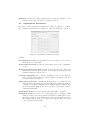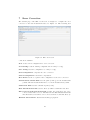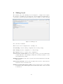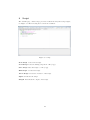
1
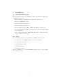
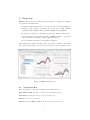
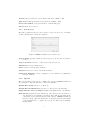
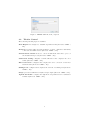
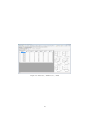
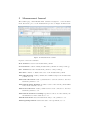
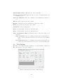
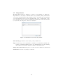
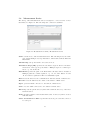
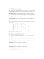
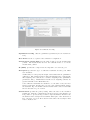
METAS VNA Tools II - User Manual V1.6 Michael Wollensack October 2015 Contents 1 Installation 1.1 System Requirements . . . . . . . . . . . . . . . . . . . . . . . . 1.2 Steps . . . . . . . . . . . . . . . . . . . . . . . . . . . . . . . . . . 3 3 3 2 Overview 2.1 Navigation Bar . . . 2.1.1 New Project 2.1.2 Options . . . 2.2 Tabular Control . . . . . . . . . . . . . . . . . . . . . . . . . . . . . . . . . . . . . . . . . . . . . . . . . . . . . . . . . . . . . . . . . . . . . . . . . . . . . . . . . . . . . . . . . . . . . . . . . . . . . . . 4 4 5 5 6 3 Data Explorer 3.1 Filetypes . . . . . . . . 3.2 File Explorer . . . . . 3.2.1 Content Menu 3.3 Visualization . . . . . 3.3.1 Graph . . . . . 3.3.2 Table . . . . . 3.3.3 Point . . . . . 3.3.4 Covariance . . 3.3.5 Info . . . . . . 3.4 Math . . . . . . . . . . 3.5 Uncertainty . . . . . . . . . . . . . . . . . . . . . . . . . . . . . . . . . . . . . . . . . . . . . . . . . . . . . . . . . . . . . . . . . . . . . . . . . . . . . . . . . . . . . . . . . . . . . . . . . . . . . . . . . . . . . . . . . . . . . . . . . . . . . . . . . . . . . . . . . . . . . . . . . . . . . . . . . . . . . . . . . . . . . . . . . . . . . . . . . . . . . . . . . . . . . . . . . . . . . . . . . . . . . . . . . . . . . . . . . . . . . . . . . . . . . . . . . . . . . . . . . . . . . . . . . . . . . . . . . . . . . . . . . . . . . . 7 7 7 7 9 9 10 12 13 14 15 16 4 Database 4.1 Cable . . . . . . . . . . . . . . . . . . . 4.2 Calibration Standard . . . . . . . . . . . 4.2.1 Agilent Model Standard . . . . . 4.2.2 Databased Standard . . . . . . . 4.2.3 New Database Standard Wizard 4.2.4 Primary Airline Standard . . . . 4.2.5 Primary Offset Short Standard . 4.2.6 Waveguide Shim Standard . . . . 4.2.7 Waveguide Offset Short Standard 4.3 Connector . . . . . . . . . . . . . . . . . 4.4 VNA Device . . . . . . . . . . . . . . . . . . . . . . . . . . . . . . . . . . . . . . . . . . . . . . . . . . . . . . . . . . . . . . . . . . . . . . . . . . . . . . . . . . . . . . . . . . . . . . . . . . . . . . . . . . . . . . . . . . . . . . . . . . . . . . . . . . . . . . . . . . . . . . . . . . . . . . . . . . . . . . . . . . . . . . . . . . 17 17 18 19 19 20 20 22 23 23 24 25 1 5 Measurement Journal 5.1 VNA Settings . . . . . . . . 5.2 Cable Movement . . . . . . 5.3 Custom Cable Settings . . . 5.4 New Connection . . . . . . 5.5 Custom Connector Settings 5.6 Measurement . . . . . . . . 5.7 Experiment . . . . . . . . . 5.8 Measurement Series . . . . 5.9 User Comment . . . . . . . . . . . . . . . . . . . . . . . . . . . . . . . . . . . . . . . . . . . . . . . . . . . . . . . . . . . . . . . . . . . . . . . . . . . . . . . . . . . . . . . . . . . . . . . . . . . . . . . . . . . . . . . . . . . . . . . . . . . . . . . . . . . . . . . . . . . . . . . . . . . . . . . . . . . . . . . . . . . . . . . . . . . . . . . . . . . . . . . . . . . . . . . . . . . . 29 30 32 32 33 34 35 36 37 38 6 Calibration Config 39 6.1 Optimization Parameters . . . . . . . . . . . . . . . . . . . . . . 41 7 Error Correction 42 8 Sliding Load 43 9 Script 44 10 Calibration Standard Model Fit 45 A File Types 46 B Naming Convention 47 C Drivers 50 D Further Reading 52 2 1 Installation 1.1 System Requirements The following list describes the minimum software and hardware requirements of METAS VNA Tools II. • Microsoft Windows XP (Windows 7 64 Bit is recommended) • Microsoft .NET Framework 3.5 • Microsoft Windows Installer 3.1 • National Instruments VISA 5.2 • At least 1024 megabytes (MB) of RAM (4096 MB is recommended) • At least 100 megabytes (MB) of available space on the hard disk (10 GB is recommended) • Video adapter and monitor with SVGA (800 x 600) or higher resolution (1920 x 1200 is recommended) 1.2 Steps The following steps describe the installation of METAS VNA Tools II. 1. Double-click on the METAS VNA Tools II setup program 2. Accept license agreement 3. Select installation folder 4. Confirm installation 5. Installation complete After the installation, one can start METAS VNA Tools II by double-clicking on its desktop shortcut. 3 2 Overview METAS VNA Tools II is a software which is designed to compute uncertainties of S-parameter measurements: • It uses a VNA measurement model for N -port Vector Network Analyzers. • It supports the following calibration types: One Port, SOLT, GSOLT, QSOLT, Unknown Thru, TRL, Juroshek, LHKM and Optimization. • It allows the definition of all influences that affect VNA measurements. • It uses the Linear Propagation module of METAS UncLib to propagate all uncertainties through the VNA measurement model. • It can visualize S-parameter data with uncertainties. The graphical user interface is split up into two parts, see Figure 1. The navigation bar is in the upper part of the screen and below is the tabular control. Figure 1: METAS VNA Tools II 2.1 Navigation Bar The following user controls are available in the navigation bar: Global Root Path sets the root directory for all tabular pages. New Project creates a new project, see section 2.1.1. Browse selects a root directory. Options sets the METAS VNA Tools II options, see section 2.1.2. 4 Console shows or hide the console window (shortcut: CTRL + F9). Split View splits the tabular control (shortcut: CTRL + F10). Create Screenshots creates screen shots of all tabular pages. About shows the about box. 2.1.1 New Project The dialog called New Project can be used to create a new project, see Figure 2. The following user controls are available: Figure 2: METAS VNA Tools II / New Project Project Name specifies a name for the new project. A new directory will be created. Project Location sets the root directory for the new project. VNA Device selects a VNA device. Cable selects a cable from the database. Connector selects a connector from the database. Calibration Template selects a template for the calibration configuration from the database. 2.1.2 Options The options dialog can be used to configure the options of METAS VNA Tools II, see Figure 3. The following user controls are available: Default Root Path sets the root directory. Default Root Path Database sets the root directory for the database. Single Instance limits the METAS VNA Tools II application to one instance. Drift Model specifies the used drift model. One can chose the Correlated or Uncorrelated model (default: Correlated). The drift model which is uncorrelated is obsolete and was used in older versions of METAS VNA Tools II (before V0.9). The new drift model (correlated) uses the time stamp of the measurement to compute how big is the drift between multiple measurements. 5 Figure 3: METAS VNA Tools II / Options 2.2 Tabular Control The following tabular pages are available: Data Explorer is designed to visualize S-parameter files (shortcut: CTRL + F1). Database specifies values and uncertainties of cables, calibration standards, connectors and VNA devices (shortcut: CTRL + F2). Measurement Journal is used to collect measurement data and to protocol the measurement process (shortcut: CTRL + F3). Calibration Config configures a VNA calibration and computes the error terms (shortcut: CTRL + F4). Error Correction configures and computes the error correction of raw measurement data (shortcut: CTRL + F5). Sliding Load configures and computes the circle fit of a sliding load (shortcut: CTRL + F6). Script provides a built-in Iron Python script engine (shortcut: CTRL + F7). Agilent Model Fit computes the Agilent model parameters for a calibration standard (shortcut: CTRL + F8). 6 3 Data Explorer The Data Explorer tabular page is designed to visualize S-parameter files. The graphical user interface is split up into two parts. The file explorer is on the left and the visualization with different tabs is on the right. 3.1 Filetypes Table 1 shows the supported file types. S-Parameter Data files can only contain Table 1: File types Description S-Parameter Data Binary S-Parameter Data Xml S-Parameter Data Covariance Text S-Parameter Data Touchstone VNA Calibration Data Binary VNA Data Binary VNA Data Xml VNA Data CITI Extension (.sdatb) (.sdatx) (.sdatcv) (.s*p) (.calb) (.vdatb) (.vdatx) (.cti;.citi) S-parameter data. In contrast VNA Data files can contain receiver values and ratios of receiver values. 3.2 File Explorer The following user controls are available: Filter sets file filter (default: *.*). Freq List Browse can be used to select a frequency list file. All selected files in the tree view will be interpolated (default: None). Freq List On turns frequency list interpolation on or off (default: Off). Tree View can be used to select one or multiple files. Additional files can be selected while holding the CTRL or SHIFT key. 3.2.1 Content Menu The content menu of the File Explorer provides some tools for post processing of data sets. All post processing tools propagate the uncertainties of the inputs to the results. The following tools are available: Show in Windows Explorer shows a file or directory in the Windows Explorer. Set as Root Path sets the current directory as root path. New Folder creates a new folder in the current directory. 7 New Shortcut creates a new shortcut in the current directory. Save Data As ... saves the current file in another file. Supported file formats are S-Parameter Data (*.sdatb or *.sdatx), Covariance Text (*.sdatcv), Touchstone (*.s1p, *.s2p, *.s*p), VNA Data (*.vdatb or *.vdatx) or CITI (*.cti or *.citi). Change Port Assignment changes the port assignment. Change Port Zr changes the reference impedance to a specified complex value in Ohm. Math provides the following math tools: Add (1st + 2nd) adds N -port 1 and N -port 2. Subtract (1st - 2nd) subtracts N -port 2 from N -port 1. Subtract (2nd - 1st) subtracts N -port 1 from N -port 2. Multiply (1st x 2nd) multiplies N -port 1 with N -port 2. Divide (1st / 2nd) divides N -port 1 by N -port 2. Divide (2nd / 1st) divides N -port 2 by N -port 1. Cascade provides the following cascade tools: Cascade (1st and 2nd) cascades 2N -port 1 with N -port 2 or cascades 2-port 1 with 2-port 2. Cascade (2nd and 1st) cascades 2N -port 2 with N -port 1 or cascades 2-port 2 with 2-port 1. Cascade (inv(1st) and 2nd) cascades inverted 2N -port 1 with N -port 2 or cascades inverted 2-port 1 with 2-port 2. Cascade (inv(2nd) and 1st) cascades inverted 2N -port 2 with N -port 1 or cascades inverted 2-port 2 with 2-port 1. Cascade (1st and inv(2nd)) cascades N -port 1 with inverted 2N -port 2 or cascades 2-port 1 with inverted 2-port 2. Cascade (2nd and inv(1st)) cascades N -port 2 with inverted 2N -port 1 or cascades 2-port 2 with inverted 2-port 1. Merge (lower and upper) merges two data sets at a given frequency point. Mean Data Set computes the mean of a data set. Circle Fit Data Set computes the circle fit of a data set. Properties shows the file or directory properties. 8 3.3 Visualization The Data Explorer supports different view modes: Graph shows a graphical visualization of multiple files. Table shows a tabular visualization of a single file. Point shows an uncertainty budget for one frequency point and one parameter of a single file. Covariance shows a covariance matrix for a single frequency point or a single parameter of a single file. Info shows file information including MD5 checksum of multiple files. 3.3.1 Graph The graph tab supports multiple selected files, see Figure 4. The following user Figure 4: Data Explorer / Graph controls are available: SetUp sets up the plots (default: Sx,x Ports: 1, 2). Conv sets the conversion to None, S/S’, Impedance, Admittance, VSWR or Time Domain (default: None). Format sets the data format to Real Imag, Mag Phase, Real, Imag, Mag, Phase or Cartesian (default: Mag Phase). Freq log sets the frequency axis to linear or logarithmic (default: Freq lin). Mag format sets the magnitude format to Mag lin (reflection and transmission linear), Mag log (reflection and transmission logarithmic) or Mag lin log (reflection linear and transmission logarithmic) (default: Mag lin). 9 Phase format sets the phase format to Phase 180, Phase 360, Phase Unwrap, Phase Delay or Group Delay (default: Phase 180). Unc sets the uncertainty mode to None, Standard or U95 (default: None). Interaction Mode sets interaction mode to None, Zoom or Pan (default: None). Fixed Scale activates or deactivates automatically scaling of the x- and y-axis. Cursor shows or hides one or two cursors. Norm normalizes all traces to one selected trace or to the mean value of all traces (default: None). In the neighboring control one can select if normalization is with respect to value or value and uncertainty. Normalizing to a value means subtracting certain values from the dataset. The resulting uncertianties are the same as from the input data. Normalizing to value and uncertainty means subtracting uncertain numbers from the dataset. The resulting uncertainties are different from the previous case because the uncertainties are as well subtracted. Font specifies the font for the current plots. Save Image saves the current plots to a bitmap file. Supported file formats are BMP, JPG and PNG. Copy Image copies the current plots to the clipboard. Table 2 shows the different colors for each trace and its associated uncertainty region. Table 2: Trace Colors Trace 1 2 3 4 5 6 7 8 9 10 3.3.2 Value Unc Color black brown red orange yellow green blue violet gray light gray Table The first of the selected files will be shown in the table view, see Figure 5. The following user controls are available: Conv sets the conversion to None, S/S’, Impedance, Admittance, VSWR or Time Domain (default: None). 10 Figure 5: Data Explorer / Table Format sets the data format to Real Imag, Mag Phase or Mag (default: Mag Phase). Mag format sets the magnitude format to Mag lin (reflection and transmission linear), Mag log (reflection and transmission logarithmic) or Mag lin log (reflection linear and transmission logarithmic) (default: Mag lin). Phase format sets the phase format to Phase 180, Phase 360, Phase Unwrap, Phase Delay or Group Delay (default: Phase 180). Unc sets the uncertainty mode to None, Standard or U95 (default: None). Freq sets the frequency format to Hz, kHz, MHz or GHz (default: MHz). Numeric Format sets the numeric format (default: f3). Save Data saves the current data in a file. Supported file formats are SParameter Data (*.sdatb or *.sdatx), Covariance Text (*.sdatcv), Touchstone (*.s1p, *.s2p, *.s*p), VNA Data (*.vdatb or *.vdatx) or CITI (*.cti or *.citi). Save Table saves the current formatted data in a file. Supported file formats are Text (*.txt) or LATEX(*.tex). Copy Table copies the current formatted data to the clipboard. One can select one or more rows of the table and copy the data to the clipboard with CTRL-C or with the context menu of the table. CTRL-A selects all data. 11 Figure 6: Data Explorer / Point 3.3.3 Point The first of the selected files will be shown in the point view. One can select one frequency point and one parameter and obtains the uncertainty budget of the selected data point, see Figure 6. The following user controls are available: Freq selects a frequency point for the uncertainty budget (default: None). Time selects a time point for the uncertainty budget (default: None). Only visible when conversation is set to Time Domain. First selects the first frequency or time point. Last selects the last frequency or time point. Parameter selects a parameter for the uncertainty budget (default: None). Conv sets the conversion to None, S/S’, Impedance, Admittance, VSWR or Time Domain (default: None). Format sets the format to Real, Imag, Mag, Mag log, Phase, Phase 360, Phase Unwrap, Phase Delay or Group Delay (default: Mag). Id shows or hides the uncertainty input ids (default: Hide). Flat shows a flat or tree uncertainty budget (default: Tree). Expand All expands all tree nodes. Collapse All collapses all tree nodes. Sort sets the sort order to Description or Uncertainty (default: Description). Copy copies the uncertainty budget to the clipboard. 12 The following items will be shown for the selected data point: Value indicates the value. Std Unc shows the standard uncertainty (68% coverage factor, k = 1). U95 shows the expanded uncertainty (95% coverage factor, k = 2). Unc Budget shows a tabular visualization of the uncertainty budget. 3.3.4 Covariance The first of the selected files will be shown in the covariance view. There are two modes in the covariance view. Either one can select a single frequency point and obtains the covariance matrix of multiple parameters at the selected frequency point. Or one can select all frequency points and a single parameter in the desired format and obtains the covariance matrix for the selected parameter and format over the hole frequency range, see Figure 7. The following user Figure 7: Data Explorer / Covariance controls are available: Freq selects a frequency point or all frequency points for the covariance view (default: None). All selects all frequency points. First selects the first frequency point. Last selects the last frequency point. Parameter selects a parameter for the covariance view (default: None). Format sets the format to Real, Imag, Mag or Phase (default: Mag). 13 Mode sets the mode to covariance or correlation (default: Covariance). Numeric Format sets the numeric format (default: e3). Color shows or hides the graphical representation of the correlation matrix (default: show). Save Table saves the current formatted covariance in a file. Supported file formats are Text (*.txt) or LATEX(*.tex). Copy Table copies the current formatted covariance to the clipboard as text. Save Image saves the current covariance to a bitmap file. Supported file formats are BMP, JPG and PNG. Copy Image copies the current covariance to the clipboard as bitmap. 3.3.5 Info The info tab supports multiple selected files. One can obtain information about multiple files by holding the CTRL or SHIFT key and selecting the files. The info tab shows the file name, size, modification date and computes the MD5 checksum for each selected file. See Figure 8. The following user controls are Figure 8: Data Explorer / Info available: Size shows or hides the file sizes (default: Show). Data modified shows or hides the file dates (default: Hide). Save Table saves the current information in a file. Supported file formats are Text (*.txt) or LATEX(*.tex). Copy Table copies the current information to the clipboard. 14 3.4 Math The same equations are used in Graph, Table and Point tab for data conversion and formatting. Table 3 shows the equations for data conversions in METAS VNA Data Explorer. Variable x is the input quantity, y is the converted ouptut, Zr is the reference impedance and Yr is the reference admittance. Index i is the frequency point, j is the receiver port and k is the source port. Table 4 shows Table 3: Conversions Conversion None S/S’ Impedance Admittance VSWR Time Domain Equation y=x yjk = xjk /xkj 1+x Zr y = 1−x 1−x y = 1+x Yr 1+|x| y = 1−|x| y = ifft (x) with 256 points the equations used for data formatting. Variable y is the converted input from Table 3 and z is the formatted output. Table 4: Formats Format Real Imag Mag Mag log Phase Phase 360 Phase Unwrap Phase Delay Group Delay Equation z = <(y) z = =(y) z = |y| z = 20 log10 (|y|) z = arg (y) z = arg (y) z = unwrap (arg (y)) ϕi zi = − 2πf with ϕ = unwrap (arg (y)) i ϕi −ϕi−1 zi = − 2π(fi −fi−1 ) with ϕ = unwrap (arg (y)) 15 3.5 Uncertainty There are three different uncertainty modes: None hides the uncertainty. Standard shows the standard uncertainty. In a scalar case this means 68% coverage and k = 1. In a two dimensional case this means 39% coverage and k = 1. U95 shows the expanded uncertainty. In a scalar case this means 95% coverage and k = 2. In a two dimensional case this means 95% coverage and k = 2.45. Here a scalar quantity consist of only one component, e.g. magnitude of Sparameter, whereas a two dimensional quantity consists of two components, e.g. complex S-parameter. In graphical representations the dimension is determined by the number of components shown in one subplot. The uncertainties are computed with linear uncertainty propagation. This leads to well known problems when computing the absolute value and phase of small quantities. 16 4 Database The Databased is designed to specify values and uncertainties of cables, calibration standards, connectors and VNA devices. 4.1 Cable The tabular page, called Cable, is designed to specify cables in the database, see Figure 9. The following user controls are available: Figure 9: Database / Cable New Cable creates a new database item of the type cable. Load Cable loads a cable from a file (*.cable). Save Cable saves the cable to a file (*.cable). Identification field can contain an identification string. Zr Real (Ohm) specifies the real part of the reference impedance in Ohm. Zr Imag (Ohm) specifies the imaginary part of the reference impedance in Ohm. Comments field can contain user comments. Electrical Specifications is a table with the following columns: • Frequency in Hz • Stability Mag (dB) with k = 2 • Stability Phase (deg) with k = 2 17 4.2 Calibration Standard The tabular page, called Calibration Standard, is designed to specify calibration standards in the database, see Figure 10. The following user controls are Figure 10: Database / Calibration Standard available: New Standard creates a new database item of the type calibration standard. For a databased standard see section 4.2.3. Load Standard loads a calibration standard from a file (*.calstd). Save Standard saves the calibration standard to a file (*.calstd). Start Frequency (Hz) specifies the start frequency. Stop Frequency (Hz) specifies the stop frequency. Points sets the number of data points. Frequency List Browse loads a frequency list. Frequency List Clear clears the frequency list. Identification field can contain an identification string. Zr Real (Ohm) specifies the real part of the reference impedance in Ohm. Zr Imag (Ohm) specifies the imaginary part of the reference impedance in Ohm. Comments field can contain user comments. 18 4.2.1 Agilent Model Standard For a calibration standard of the type Agilent model the following controls are available: Standard Type specifies the standard type as open, short, load or delay/thru. Offset Z0 (Ohm) sets the offset line impedance in Ohm. Offset Delay (ps) sets the offset line delay in ps. Offset Loss (GOhm/s) set the offset line loss in GOhm/s. CO (E-15 F) sets the first polynomial coefficient for an open. C1 (E-27 F/Hz) sets the second polynomial coefficient for an open. C2 (E-36 F/Hzˆ2) sets the third polynomial coefficient for an open. C3 (E-45 F/Hzˆ3) sets the fourth polynomial coefficient for an open. L0 (E-12 H) sets the first polynomial coefficient for a short. L2 (E-24 H/Hz) sets the second polynomial coefficient for a short. L2 (E-33 H/Hzˆ2) sets the third polynomial coefficient for a short. L3 (E-42 H/Hzˆ3) sets the fourth polynomial coefficient for a short. Electrical Specifications is a table with the following columns for an open or a short: • Frequency in Hz • Phase Deviation (deg) with k = 2 Phase deviations are as well translated to magnitude uncertainties. The used formalism yields a circular uncertainty region. For a load or delay/thru the table has the following columns: • Frequency in Hz • Return Loss (dB) with k = 2 E.g. an uncertainty of the Return Loss of -40 dB is translated to an uncertainty of 0.01 of real and imaginary part of the reflection coefficient. 4.2.2 Databased Standard Databased standards define the value and uncertainty budget of each frequency point and parameter. This format works without loss of accuracy. Thus it is ideal for transferring measurement data and uncertainties from National Metrology Institutes to customers. For a databased standard the following control is available: Data Path specifies the file path (*.sdatb) which contains the S-parameters of the standard. 19 4.2.3 New Database Standard Wizard The wizard called New Database Standard is designed to create a new databased standard, see Figure 11. The following user controls are available: Figure 11: Database / New Database Standard Wizard Data Path for Definition of Calibration Standard specifies the source file (*.sdatb) for the definition of the calibration standard. Database Path specifies the destination in the database (Example: 3.5mm\Loads\MM123456 Load(f) 789). Identification field can contain an identification string (Example: 3.5 mm female load SN:789). Date sets the date. This date is part of the name of the databased standard. 4.2.4 Primary Airline Standard For a primary airline standard the following controls are available: Material Parameters specifies the following parameters: Relative Permittivity of Air specifies the value and the uncertainty (k = 2) of the relative permittivity of air. Relative Permeability of Air specifies the value and the uncertainty (k = 2) of the relative permeability of air. DC Conductivity of Metal (S/m) specifies the value and the uncertainty (k = 2) of the DC conductivity of metal in S/m. HF Conductivity of Metal (S/m/GHzˆ0.5) specifies the value and the uncertainty (k = 2) of the HF conductivity of metal in S/m/GHzˆ0.5. Misc specifies the following parameter: Line Shift (m) specifies the value and the uncertainty (k = 2) of the distance in m which the center conductor protrudes in the test port. If the center conductor protrudes in port 1 this number is positive. In the opposite case it must be negative. If no protrusion happens, the value is zero. Connector 1 specifies the gender and the mechanical dimensions of the connector 1. The following controls are are available: 20 Gender specifies the gender (female, male or none) of the connector. Pin Depth (m) sets the value and uncertainty (k = 2) of the pin depth of the standard in m. Pin Gap (m) sets the value and uncertainty (k = 2) of the pin gap used for the simulation of the connector in m. Female Outer Chamfer (m) sets the value and uncertainty (k = 2) of the outer chamfer for a female connector in m. Female Inner Chamfer (m) sets the value and uncertainty (k = 2) of the inner chamfer for a female connector in m. Male Outer Chamfer (m) sets the value and uncertainty (k = 2) of the outer chamfer for a male connector in m. Male Inner Chamfer (m) sets the value and uncertainty (k = 2) of the inner chamfer for a male connector in m. Pin Diameter (m) sets the value and uncertainty (k = 2) of the pin diameter in m. For a female connector this should be set to the nominal value of the connector family. Hole Diameter (m) sets the value and uncertainty (k = 2) of the hole diameter in m. For a male connector this should be set to the value of the pin diameter. OC Diameter (m) sets the value and uncertainty (k = 2) of the outer conductor diameter in m. This should be set to the nominal value of the connector family. Male CC Diameter (m) sets the value and uncertainty (k = 2) of the diameter of the male center conductor in m. For a female connector this should be set to the nominal value of the connector family. Number of Slots specifies the number of slots. Zero means slotless. Slotless Hole Length (m) sets the value and uncertainty (k = 2) of the hole length in m for a slotless female connector. Slotless Female CC Diameter (m) sets the value and uncertainty (k = 2) of the center conductor diameter in m for a slotless female connector. For a male connector this should be set to the nominal value of the connector family. Slot Length (m) sets the value and uncertainty (k = 2) of the slot length in m for a slotted female connector. The slot length must be a multiple of the length of a single line section. Slot Width (m) sets the value and uncertainty (k = 2) of the slot width in m for a slotted female connector. Line Section specifies the length of the standard and the diameter profile of the line section. The following controls are available: Length (m) specifies the value and the uncertainty (k = 2) of the distance between the reference planes of connector 1 and 2. Table Diameter Profile is a table with the following columns: • z-Position (m) 21 • • • • • U(z-Position) (m) with k = 2 ICOD (m) U(ICOD) (m) with k = 2 OCID (m) U(OCID) (m) with k = 2 Graph Diameter Profile shows a graphical visualization of the diameter profile. Connector 2 specifies the gender and the mechanical dimensions of the connector 2. For the available controls see Connector 1. For a primary airline standard the following precomputed data is needed, see figure 12. Database/CalibrationStandards/[ConnectorFamily]/Primary/[name] [name].calstd .............................. primary airline standard data......................directory for precomputed S-parameter data [name] c1.sdatb.......simulated connector (female-male) at port 1 [name] c2.sdatb.......simulated connector (female-male) at port 2 [name] k1.sdatb......kapton or adapter effect on port 1 (optional) [name] k2.sdatb......kapton or adapter effect on port 2 (optional) [name] pg1.sdatb.....simulated nominal pin gap (10 µm) at port 1 [name] pg2.sdatb.....simulated nominal pin gap (10 µm) at port 2 Figure 12: Precomputed data for a primary airline standard 4.2.5 Primary Offset Short Standard For a primary offset short standard the following controls are available: Material Parameters specifies the material parameters. Connector specifies the gender and the mechanical dimensions of the connector. Line Section specifies the length between the reference plane in the connector and the short plane. The diameter profile of the line section is specified as well. For more details, see section 4.2.4. For a primary offset short the following precomputed data is needed, see figure 13. Database/CalibrationStandards/[ConnectorFamily]/Primary/[name] [name].calstd..........................primary offset short standard data......................directory for precomputed S-parameter data [name] c1.sdatb................simulated connector (female-male) [name] k1.sdatb................kapton or adapter effect (optional) [name] pg1.sdatb..............simulated nominal pin gap (10 µm) Figure 13: Precomputed data for a primary offset short standard 22 4.2.6 Waveguide Shim Standard For a waveguide shim standard the following controls are available: Material Parameters specifies the following parameters: Relative Permittivity of Air specifies the value and the uncertainty (k = 2) of the relative permittivity of air. Relative Permeability of Air specifies the value and the uncertainty (k = 2) of the relative permeability of air. DC Conductivity of Metal (S/m) specifies the value and the uncertainty (k = 2) of the DC conductivity of metal in S/m. HF Conductivity of Metal (S/m/GHzˆ0.5) specifies the value and the uncertainty (k = 2) of the HF conductivity of metal in S/m/GHzˆ0.5. Waveguide Connector 1 specifies the mechanical dimensions of the connector 1. The following controls are are available: Test Port Width (m) specifies the nominal width of the test port in m. Test Port Height (m) specifies the nominal height of the test port in m. Waveguide Shim Section specifies the length of the standard and the mechanical dimensions of the shim section. The following controls are available: Length (m) sets the value and the uncertainty (k = 2) of the length of the shim section in m. Width (m) sets the value and the uncertainty (k = 2) of the width of the shim section in m. Height (m) sets the value and the uncertainty (k = 2) of the height of the shim section in m. Radius (m) sets the value and the uncertainty (k = 2) of the radius of the shim section in m. Width Offset (m) sets the value and the uncertainty (k = 2) of the width offset of the shim section in m. Height Offset (m) sets the value and the uncertainty (k = 2) of the height offset of the shim section in m. Waveguide Connector 2 specifies the mechanical dimensions of the connector 2. For the available controls see Waveguide Connector 1. 4.2.7 Waveguide Offset Short Standard For a waveguide offset short standard the following controls are available: Material Parameters specifies the material parameters. Waveguide Connector specifies the mechanical dimensions of the connector. 23 Waveguide Shim Section specifies the length between the reference plane in the connector and the short plane. The mechanical dimensions of the shim section are specified as well. For more details, see section 4.2.6. 4.3 Connector The Connector tabular page is designed to specify connectors in the database, see Figure 14. The following user controls are available: Figure 14: Database / Connector New Connector creates a new database item of the type connector. Load Connector loads a connector from a file (*.conn). Save Connector saves the connector to a file (*.conn). Identification field can contain an identification string. Zr Real (Ohm) specifies the real part of the reference impedance in Ohm. Zr Imag (Ohm) specifies the imaginary part of the reference impedance in Ohm. Comments field can contain user comments. Electrical Specifications is a table with the following columns: • Frequency in Hz • Repeatability (dB) with k = 2 24 4.4 VNA Device The VNA Device tabular page is designed to specify VNA devices in the database, see Figure 15. The following user controls are available: Figure 15: Database / VNA Device / Settings New VNA creates a new database item of the type VNA device. Load VNA loads a VNA item from a file (*.vnadev). Save VNA saves the VNA item to a file (*.vnadev). Test Device tests VNA device if VISA connection is possible. Characterize Noise characterize the noise of the VNA at the specified frequency points, average factor, IF bandwidth and power level. The following user controls are available on the sub tabular page called Settings: Identification field can contain an identification string. Zr Real (Ohm) specifies the real part of the reference impedance in Ohm. Zr Imag (Ohm) specifies the imaginary part of the reference impedance in Ohm. Driver sets the driver for the communication with the VNA device. Resource sets the VISA resource name of the VNA device. VISA resources are the addresses of devices connected to the computer. VISA is a standard which is accepted by nearly all manufactures of VNAs. Number of Test Ports specifies the number of test ports. Comments field can contain user comments. 25 Spec Average Factor specifies the average factor used for the noise specification. Spec IF Bandwidth (Hz) specifies the IF bandwidth used for the noise specification. Spec Power (dBm) specifies the power level used for the noise floor and linearity specification. The next sub tabular page is called Noise, see Figure 16. It contains a table with the following columns: Figure 16: Database / VNA Device / Noise • Frequency (Hz) • Noise Floor (dB) with k = 2 • Trace Noise Mag (db rms) with k = 1 • Trace Noise Floor (deg rms) with k = 1 The next sub tabular page contains two tables and is called Linearity, see Figure 17. The first specifies the different power levels in dB. The second table contains the following columns: • Frequency (Hz) • Linearity Mag (dB) with k = 2, one column for each power level • Linearity Phase (deg) with k = 2, one column for each power level The next sub tabular page is called Drift, see Figure 18. It contains a table with the following columns: 26 Figure 17: Database / VNA Device / Linearity • Frequency (Hz) • Switch Term Drift (dB) with k = 2 • Directivity Drift (db) with k = 2 • Tracking Drift Mag (dB) with k = 2 • Tracking Drift Phase (deg) with k = 2 • Match Drift (dB) with k = 2 • Isolation Drift (dB) with k = 2 27 Figure 18: Database / VNA Device / Drift 28 5 Measurement Journal The tabular page, called Measurement Journal, is designed to collect measurement data and to protocol the measurement process, see Figure 19. The follow- Figure 19: Measurement Journal ing user controls are available: New Journal creates a new measurement journal. Load Journal loads an existing measurement journal from a file (*.vnalog). Save Journal saves the measurement journal to a file (*.vnalog). Auto Save enables or disables auto save of the measurement journal. Add VNA Settings adds a journal item for VNA settings to the measurement journal, see 5.1. Add Cable Movement adds a journal item for cable movement to the measurement journal, see 5.2. Add Custom Cable Settings specifies a cable for the current journal which is not in the database, see 5.3. Add New Connection adds a journal item for a new connection to the measurement journal, see 5.4. Add Custom Connector Settings specifies a connector for the current journal which is not in the database, see 5.5. Add Measurement adds a measurement entry to the journal, see 5.6. Add Begin Experiment defines the start of an experiment, see 5.7. 29 Add End Experiment defines the end of an experiment. Add Measurement Series adds an entry for a series of measurements to the journal, see 5.8. Add User Comment adds a user comment to the measurement journal, see 5.9. Edit shows the selected item of the journal. Rename renames the selected measurement item of the journal. Delete deletes the selected items of the journal. VNA Device selects a VNA device. Open opens the VISA connection to the VNA device. Close closes the VISA connection to the VNA device. Cable and Connector Table specifies the test port cable and connector for each port. Cable movement adds one or multiple entries in the measurement journal for cable movements at the selected ports before the measurement. New connection adds one or multiple entries in the measurement journal for new connections at the selected ports before the measurement. 5.1 VNA Settings The dialog, called VNA Settings, is designed to set up the VNA, see Figure 20. The following user controls are available: Figure 20: Measurement Journal / VNA Settings 30 Time Stamp specifies the time stamp for the journal item. VNA Device specifies the VNA device. Preset presets the VNA. Save Instrument State saves the instrument state from the VNA to a file (*.is). Recall Instrument State recalls the instrument state from a file (*.is) to the VNA. Refresh refresh all settings from the VNA. Sweep Mode sets the sweep mode to linear frequency, log frequency, segment sweep or CW time. Sweep Time (s) sets the sweep time in s. Dwell Time (s) sets the dwell time in s. IF Average Factor sets the average factor. Start Frequency (Hz) sets the start frequency in Hz. Stop Frequency (Hz) sets the stop frequency in Hz. Points sets the number of sweep points. IF Bandwidth (Hz) sets the IF bandwidth in Hz. Center Frequency (Hz) sets the center frequency in Hz. Frequency Span (Hz) sets the frequency span in Hz. CW Frequency (Hz) sets the frequency for CW sweep mode in Hz. New Table creates a new segment table. Open Table loads a segment table from a file (*.txt). Save Table saves the segment table to a file (*.txt). Set Segment Table sets the segment table to the VNA. Segment Table is a table with the following columns: • Start Frequency in Hz • Stop Frequency in Hz • Step Size in Hz • IF Bandwidth in Hz System Z0 (Ohm) specifies the reference impedance in Ohm. Source 1 Power (dBm) sets the power level of the first source in dBm. Source 1 Slope (dB/GHz) sets the slope of the first source in dB/GHz. 31 Source 2 Power (dBm) sets the power level of the second source in dBm. Source 2 Slope (dB/GHz) sets the slope of the second source in dB/GHz. Port 1 Attenuator (dB) sets the attenuation of the first port in dB. Port 1 Extension (s) shifts the reference plane of port 1 by a definable delay in s. Port 2 Attenuator (dB) sets the attenuation of the second port in dB. Port 2 Extension (s) shifts the reference plane of port 2 by a definable delay in s. 5.2 Cable Movement The dialog, called Cable Movement, is designed to describe a cable movement for the journal, see Figure 21. The following user controls are available: Figure 21: Measurement Journal / Cable Movement Time Stamp specifies the time stamp of the journal item. Cable selects a cable from the database. Port specifies at which port the cable was moved. Position specifies the position of the cable. Thus each cable movement requires an increase of the position number. With each change of the position number the cable uncertainties, specified in the database, are added to the measurement data. 5.3 Custom Cable Settings The dialog, called Custom Cable Settings, is designed to describe cables which are not in the database for the current journal. One can specify the magnitude and phase stability of such a cable in this dialog, see Figure 22. The following user controls are available: Time Stamp specifies the time stamp of the journal item. Identification field contains identification string. Zr Real (Ohm) specifies the real part of the reference impedance in Ohm. 32 Figure 22: Measurement Journal / Custom Cable Settings Zr Imag (Ohm) specifies the imaginary part of the reference impedance in Ohm. Comments field can contain user comments. Electrical Specifications is a table with the following columns: • Frequency in Hz • Stability Mag (dB) with k = 2 • Stability Phase (deg) with k = 2 Import Cable imports a cable from the database. 5.4 New Connection The dialog, called New Connection, is designed to describe a new connection in the journal, see Figure 23. The following user controls are available: Figure 23: Measurement Journal / New Connection Time Stamp specifies the time stamp of the journal item. Connector selects a connector from the database. Port specifies at which port the new connection was made. 33 5.5 Custom Connector Settings The dialog, called Custom Connector Settings, is designed to describe a connector which is not in the database for the current journal. One can specify the repeatability of such a connector in this dialog, see Figure 24. The following Figure 24: Measurement Journal / Custom Connector Settings user controls are available: Time Stamp specifies the time stamp of the journal item. Identification field can contain an identification string. Zr Real (Ohm) specifies the real part of the reference impedance in Ohm. Zr Imag (Ohm) specifies the imaginary part of the reference impedance in Ohm. Comments field can contain user comments. Electrical Specifications is a table with the following columns: • Frequency in Hz • Repeatability (dB) with k = 2 Import Connector imports a connector from the database. 34 5.6 Measurement The Measurement dialog is designed to collect measurement data from the VNA, see Figure 25. The following user controls are available: Figure 25: Measurement Journal / Measurement Time Stamp specifies the time stamp of the journal item. VNA Device specifies the VNA device. Path field contains the path of the measurement data. Import imports an existing file instead of making a new VNA measurement. Only available if VNA connection is closed. Mode selects a setup mode for the VNA, e.g. S1,1. SetUp sets up the VNA to the selected mode. Measure performs a single sweep on the VNA, wait until the sweep is complete and reads out the data. Trigger Single performs a single sweep on the VNA and waits until the sweep is complete. Trigger Cont sets the trigger of the VNA to continuous mode. Trigger Hold sets the trigger of the VNA to hold mode. Trigger Cancel cancels the current sweep. Format sets the format to Raw Data or Error Corrected Data (default: Raw Data). Get Data reads out the data from the VNA. Save Data saves the data to an S-parameter file (*.sdatb). 35 5.7 Experiment The Experiment dialog is designed to describe an experiment, see Figure 26. Experiments are necessary for DUTs with bad repeatability. The journal items of the type experiment will cause VNA Tools II to determine the repeatability of the measurement from repeated measurements. If no journal items of the type experiment are used, the repeatability uncertainties from the database will be used. The following user controls are available: Figure 26: Measurement Journal / Experiment Time Stamp specifies the time stamp of the journal item. Type sets the type of the experiment to Statistical or Systematic (default: Systematic). Statistical assumes a mono modal distribution for the resulting uncertainties. Systematic assumes a multi modal distribution. Independet S-Parameters ignores correlation between different S-Parameters. Comments field can contain user comments. 36 5.8 Measurement Series The dialog, called Measurement Series, is designed to collect a series of measurements, see Figure 27. The following user controls are available: Figure 27: Measurement Journal / Measurement Series Mode sets the mode of the measurement series. The following modes are available: DUT, Sliding Load, Step Attenuator, Switch States, ECal, Drift and ECal Drift. VNA SetUp sets up the VNA to the selected mode. Attenuator Steps (dB) specifies the attenuator steps in dB for a measurement series of the type step attenuator. Multiple steps are comma separated, e.g. ‘10, 20, 40, 40’. ECal Path specifies the path of the ECal where all states will be measured. Multiple paths are comma separated, e.g. ‘A’, ‘B’, ‘AB’. Where ‘A’ and ‘B’ are reflection paths and ‘AB’ is a transmission path. Driver sets the driver for the communication with the Switch or ECal device. Resource sets the VISA resource name of the Switch or ECal device. Open opens the VISA connection to the Switch or ECal device. Close close the VISA connection to the Switch or ECal device. Directory sets the parent directory that will contain the directory of the measurement series. Name specifies a name for the measurement series. A directory will be created with this name. Cable and Connector Table specifies the used test port cable and connector for each port. 37 Cable movement adds one or multiple entries for cable movements at the selected ports in the measurement journal before the measurement series. New connection adds one or multiple entries for new connections at the selected ports in the measurement journal before the measurement series. Delay (s) sets the delay between switching states and start of the measurements in s (default: 1 s). Number of toggles sets the number of switching cycles that are performed on the step attenuator before the measurement series is started (default: 10). Period (s) sets the period between measurements for drift evaluation in s (default: 900 s). Number of measurements sets the number of measurements for drift evaluations (default: 96). Switch states sets the list of switch states which will be measured. Each line in this text box specifies one state. ‘0’ is off, ‘1’ is on and ‘x’ is don’t change. 5.9 User Comment The dialog, called User Comment, is designed to add user comments to the journal, see Figure 28. The following user controls are available: Figure 28: Measurement Journal / User Comment Time Stamp specifies the time stamp of the journal item. Comments field can contain user comments. 38 6 Calibration Config The tabular page, called Calibration Config, is designed to configure a VNA calibration. The result will be the switch and error terms of the VNA. There are two models of the VNA: Generic Model stores the switch terms in a N -port and the error terms are stored in a 2N -port for a N -port VNA. For a two port VNA, this calibration model is known as 7-term model. It supports the following calibration types: One Port, GSOLT, QSOLT, Unknown Thru, TRL (only 2-port), Juroshek, LHKM and Optimization. Switched Model stores the error terms in a 2N -port for each switch position for a N -port VNA. For a two port This model is used for the SOLT calibration. The following S-parameter matrix N -port VNA. D1 X1,2 X2,1 D2 .. . XN,1 XN,2 T,1 T,2 .. . describes the calibration error terms of a X1,N X2,N T1, T2, .. . DN TN, M1 M2 .. . T,N MN Dx denotes the directivity of port x. Xy,x denotes the crosstalk from port x to port y. Tx,x denotes the reflection tracking of port x. Ty,x denotes the transmission tracking from port x to port y where Ty,x = Ty, T,x . Mx denotes the match of port x and all other terms are additional crosstalk terms. On the tabular page, called Calibration Config, the following user controls are available, see Figure 29: New Config creates a new calibration configuration. New Config from Template loads a configuration template. Load Config loads an existing configuration from a file (*.calcfg). Save Config saves the configuration to a file (*.calcfg). Start Computation computes the VNA calibration and saves the VNA calibration to a file (*.calb). Cancel Computation cancels the computation. 39 Figure 29: Calibration Config Optimization Config edits the optimization parameters (not in external version). Root Path sets the root path for the calibration configuration . Measurement Journal Path sets the path (*.vnalog) for the measurement journal. All measurements used for the calibration have to be in the measurement journal. Zr (Ohm) specifies the complex reference impedance for each test port. Description specifies the type of calibration standard and the ports which were measured. Additionally one can specify the weight of the standard in an optimization calibration. The default setting is that all standards have equal weight. The weighting can be switched to covariance weighting in the optimization parameters dialog. Mathematical details about weighting schemes are given in VNA Tools II - Math Reference. Some calibration standards are assumed to be the same or they are measured several times. In such cases one can couple variables which describe the standard. E.g.: In an LRL calibration with 7 mm connectors the flush short is the same for port 1 and 2. Measurement specifies the path (*.sdatb) where the data of the measured standard is. Only the configuration (*.slcfg) is given for the sliding load. It is possible to specify an N -port file for 1-port standards. In such a case the number in the description field defines which part of the data is used. E.g. only S1,1 of a 2-port file is used in a line where the description field is set to Reflection 1. 40 Definition specifies the path (*.calstd) which contains the definition of the standard. Leave this cell empty for a switch term row. 6.1 Optimization Parameters The dialog, called Optimization Calibration Config, is designed to configure the optimization parameters, see Figure 30. The following user controls are Figure 30: Optimization Calibration Config available: Set Mask Error Terms sets the mask of the error terms for a non-, half- or full-leaky model of the VNA. Start Calibration Path specifies the start values used for the optimization (*.calb). Reduced Frequency List Path specifies a frequency list (*.fl). The optimizer uses the listed frequency points. If no frequency list is specified, all available frequency points are used. Covariance Weighting uses covariance weighting for the objective function. If not checked, all standards are equally weighted it’s supplied, the user specified weights are applied. All Frequencies At Once optimizes all frequencies at once. This is needed when calibration standards are used with unknown parameters which are constant over frequency. Example given: Primary airlines, primary offset shorts and primary flush shorts. If not checked, each frequency will be optimized individually. Mask Switch Terms selects the switch terms which will be optimized. Mask Error Terms selects the error terms which will be optimized. This mask represents a 2N × 2N S-parameter matrix for a VNA with N ports. In the upper left part of the matrix are the directivity and isolation terms. The match terms are in the lower right of the diagonal. The other check boxes represent tracking terms. 41 7 Error Correction The tabular page, called Error Correction, is designed to configure the error correction of the raw measurement data, see Figure 31. The following user Figure 31: Error Correction controls are available: New creates a new configuration for error correction. Load Config loads an existing configuration from a file (*.corcfg). Save Config saves the configuration to a file (*.corcfg). Start Computation computes the error correction. Cancel Computation cancels the computation. Root Path sets the root path for the configuration of the error correction. Measurement Journal Path sets the path (*.vnalog) for the measurement journal. All raw measurements have to be in the measurement journal. Calibration Path sets the calibration path (*.calb). Raw Measurement Path sets the directory which contains the raw data. Error Corrected Measurement Path specifies the path where the errorcorrected data will be stored. All files from the Raw Measurement Path and all subdirectories will be error-corrected and stored in this directory. Without Uncertainties disables uncertainty propagation. 42 8 Sliding Load The tabular, page called Sliding Load, is designed to configure and compute the circle fit of a sliding load. It merges the circle fit with the measurement of a low-band load at the specified frequency point, see Figure 32. The following Figure 32: Sliding Load user controls are available: New creates a new configuration for a sliding load. Load Config loads an existing configuration from a file (*.slcfg). Save Config saves the configuration to a file (*.slcfg). Root Path sets the root path for the configuration. Measurement Journal Path sets the path (*.vnalog) for the measurement journal. The files of the sliding load and the low-band load have to be in the measurement journal. Sliding Load Path sets the directory where the raw measurements of the sliding load are. Lowband Load Path sets the path (*.sdatb) where the file of the raw measurement of the low-band load is. Sliding Load Start Frequency (Hz) sets the start frequency of the sliding load in Hz. Below this frequency the measurement data of the low band load is used. 43 9 Script The tabular page, called Script, provides a built-in Iron Python script engine, see Figure 33. The following user controls are available: Figure 33: Script New Script creates a new script. Load Script loads an existing script from a file (*.py). Save Script saves the script to a file (*.py). Run Script executes the script. Abort Script aborts the execution of the script. Input field shows the script. Output field shows the output of the script. 44 10 Calibration Standard Model Fit The tabular page, called Cal Std Model Fit, computes the parameters of a calibration standard for an Agilent, Anritsu and Rohde Schwarz model, see Figure 34. The following user controls are available: Figure 34: Calibration Standard Model Fit Load Data loads S-parameter file (*.sdatb). Start Optimization starts optimization of the selected parameters. Cancel Optimization aborts optimization. Copy Result copies the result to the clipboard. Start Agilent Definition describes the start values for the optimization. Mask selects optimization parameters. Agilent Definition shows the result for the Agilent model. Agilent Fit Error shows the fit error for the Agilent model. Anritsu Definition shows the result for the Anritsu model. Anritsu Fit Error shows the fit error for the Anritsu model. Rohde Schwarz Definition shows the result for the Rohde Schwarz model. Rohde Schwarz Fit Error shows the fit error for the Rohde Schwarz model. 45 A File Types Table 5 shows the supported file types. S-Parameter Data files can only contain S-parameter data. In contrast VNA Data files can contain receiver values and ratios of receiver values. Table 5: File types Description S-Parameter Data Binary S-Parameter Data Xml S-Parameter Data Covariance Text S-Parameter Data MMS4 DSD Text1 S-Parameter Data Touchstone VNA Calibration Config VNA Calibration Data Binary VNA Calibration Data Xml VNA Data Binary VNA Data Xml VNA Data CITI VNA Database Cable VNA Database Calibration Standard VNA Database Connector VNA Database VNA Device VNA Error Correction Config VNA Measurement Journal VNA Sliding Load Config Frequency List 1 readonly 46 Extension (.sdatb) (.sdatx) (.sdatcv) (.dsd) (.s*p) (.calcfg) (.calb) (.calx) (.vdatb) (.vdatx) (.cti;.citi) (.cable) (.calstd) (.conn) (.vnadev) (.corcfg) (.vnalog) (.slcfg) (.fl) B Naming Convention The here described naming convention is meant as a help for the user. It is not required by VNA Tools II. Table 6 shows some examples for the naming convention. Table 6: Naming convention examples Description Coaxial DUT Coaxial DUT Waveguide DUT Waveguide DUT Name ’[DUT][Gender] [SN]’ ’[DUT] [Conn 1][Gender 1] [Conn 2][Gender 2] [SN]’ ’[DUT] [SN] [Orientation]’ ’[DUT] [Conn] [SN] [Orientation]’ Table 7 shows some examples for names of calibration standards and devices under test. Table 8 shows the naming convention for the different connector Table 7: DUT types Description Open Short (n) Flush Short Load Sliding Load Mismatch Power Sensor Thru Line l mm Shim Adapter Matching Pad Match Thru Mismatch Thru Attenuator a dB Step Attenuator a dB, selected state: s, x dB Splitter Coupler Name ’Open’ ’Short[n]’ ’FShort’ ’Load’ ’SLoad’ ’MMatch’ ’PSensor’ ’Thru’ ’Line[l]mm’ ’Shim’ ’Ada’ ’MPad’ ’MThru’ ’MmThru’ ’Att[a]dB’ ’StepAtt[a]dB [s] [x]dB’ ’Splitter’ ’Coupler’ types. Table 9 shows the naming convention for the gender of connectors. Table 10 shows the naming convention for the orientation of waveguides. Figure 35 shows a typical project example. 47 Table 8: Connector types Description 1.0 mm Connector 1.85 mm Connector 2.4 mm Connector 2.92 mm Connector 3.5 mm Connector 7 mm Connector BNC 50 Ω Connector Type N 50 Ω Connector Type N 75 Ω Connector Waveguide WR10 Connector Name ’1.0mm’ ’1.85mm’ ’2.4mm’ ’2.92mm’ ’3.5mm’ ’7mm’ ’BNC50’ ’N50’ ’N75’ ’WR10’ Table 9: Gender of connectors Description 1-Port DUT female 1-Port DUT male 2-Port DUT female male 2-Port DUT male female N-Port DUT female male male . . . N-Port DUT genderless Name ’(f)’ ’(m)’ ’(f-m)’ ’(m-f)’ ’(f-m-m-. . .)’ ” Table 10: Orientation of waveguides Description 1-Port DUT 1-Port DUT 1-Port DUT 1-Port DUT 2-Port DUT 2-Port DUT 2-Port DUT 2-Port DUT 2-Port DUT 2-Port DUT 2-Port DUT 2-Port DUT label label label label label label label label label label label label up down left right up on test port side 1 down on test port side 1 left on test port side 1 right on test port side 1 up on test port side 2 down on test port side 2 left on test port side 2 right on test port side 2 48 Name ’U’ ’D’ ’L’ ’R’ ’U1’ ’D1’ ’L1’ ’R1’ ’U2’ ’D2’ ’L2’ ’R2’ Example 2.4mm(f-m) 01 ................................ project directory Measurements 01...........................................raw data CalStandards SLoad(f) 1567 01 SLoad(f) 1567 01 N1.sdatb SLoad(f) 1567 01 N2.sdatb ... SLoad(m) 1763 01 SLoad(m) 1763 01 N1.sdatb SLoad(m) 1763 01 N2.sdatb ... Load(f) 451 Load(m) 3218 01.sdatb Open(f) 975 Open(m) 999 01.sdatb Short(f) 747 Short(m) 2887 01.sdatb SwitchTerms 01.sdatb Thru 01.sdatb DUTs Ada 2.4mm(f) 1.85mm(m) 123 01.sdatb Att20dB(f-m) 808 01.sdatb ... SOLT 01 out ...................................... error correted data CalStandards DUTs Ada 2.4mm(f) 1.85mm(m) 123 01.sdatb Att20dB(f-m) 808 01.sdatb ... UThru 01 out ..................................... error correted data CalStandards DUTs Ada 2.4mm(f) 1.85mm(m) 123 01.sdatb Att20dB(f-m) 808 01.sdatb ... Journal 01.vnalog ............................. measurement journal SlidingLoad 01.slcfg.............................sliding load config SlidingLoad 02.slcfg.............................sliding load config SOLT 01.calb........................................calibration data SOLT 01.calcfg .................................... calibration config SOLT 01.corcfg................................error correction config UThru 01.calb.......................................calibration data UThru 01.calcfg...................................calibration config UThru 01.corcfg .............................. error correction config Figure 35: Tree view of a VNA Tools II project example 49 C Drivers The following VNA’s are supported by METAS VNA Tools II: • Agilent 8719D/ES, 8720D/ES, 8722D/ES (Firmware: 8722ES 07.74) • Agilent 8753B/C/D/E/ES (Firmware: 8753B 03.00, 8753D 06.14) • Agilent ENA Series (Firmware: E5061B A.02.06, E5071C A.09.60) • Agilent PNA Series (Firmware: E836x & N52xx A.09.40, E5080B A.11.00)1 • Anritsu VectorStar (Firmware: MS46040A 1.7.5, MS46040B 2.1.0)1 • Hewlett Packard 8510C (Firmware: 07.14 Aug 26 1998) • Hewlett Packard 8751A (Firmware: 5.00 Mar 7 1993) • Rohde & Schwarz ZNB, ZNC, ZND, ZNBT (Firmware: 1.94)1 • Rohde & Schwarz ZVA, ZVB, ZVT (Firmware: 3.20)1 • Rohde & Schwarz ZVC, ZVK, ZVM, ZVR (Firmware: 3.55) The following switch drivers are supported by METAS VNA Tools II: • Agilent 11713A/C The following electronic calibration units are supported: • Agilent ECal connected to an Agilent PNA Series VNA. • Anritsu Autocal connected to an Anristu VectorStar VNA. Driver Development For VNA’s, switch drivers and electronic calibration units that are not supported yet, the user has the possibility to develop custom drivers that can be used with METAS VNA Tools II. This section describes the development of such drivers. The minimum software requirements for driver development in Microsoft Visual Studio for METAS VNA Tools II are: • METAS VNA Tools II, www.metas.ch/vnatools • National Instruments VISA 5.2, www.ni.com/visa • Microsoft Visual C# 2008 Express Edition, www.microsoft.com/express The step by step procedure for the development of a custom driver for a VNA is as follows: 1. Check if the environment variable called %Public% is defined. This is the case under Microsoft Windows Vista and 7 but not under XP. Under Microsoft Windows XP you have to set the %Public% variable to C:\Documents and Settings\All Users. 1 two-port and multiport 50 2. Make sure the driver template Metas.Instr.Driver.Template.zip is in the template folder of Visual Studio under %Userprofile%\Documents\ Visual Studio 2008\Templates\ProjectTemplates. Otherwise copy it from %Public%\Documents\Metas.Instr\Drivers. 3. Launch Microsoft Visual C# 2008 Express Edition. 4. Create new project from template in Visual Studio under File / New Project / My Templates / Metas.Instr.Driver.Template and name the project e.g. ‘MyFirstVNA’. 5. Add a new class to the project under Project / Add Class and name it e.g. ‘MyFirstVNA’. 6. This step describes the programming of the driver. Declare the class as public and implement the ‘Metas.Instr.Driver.Vna.IVna’ interface. See Figure 36 and MSDN website for how to implement an interface. 7. Compile project under Build / Build Solution. Make sure that the postbuild event is successful and that the MyFirstDriver.dll is copied to %Public%\Documents\Metas.Instr\Drivers. 8. Test your driver directly in METAS VNA Tools II or debug it in Microsoft Visual Studio under Debug / Start Debugging. For more help take a look at the already implemented drivers for METAS VNA Tools II under %Public%\Documents\Metas.Instr\Drivers\Source. Figure 36: MyFirstVNA - Microsoft Visual C# 2008 Express Edition: Clicking with the right mouse button on IVna opens a content menu. Clicking on the menu item Implement Interface will create the basic class structure with all necessary properties and methods for the new driver. 51 D Further Reading Documentations • VNA Tools II - User Manual • VNA Tools II - Math Reference • Data Explorer - User Manual Presentations • VNA Tools II - Overview • VNA Tools II - S-Parameter Uncertainty Calculation • VNA Tools II - Data Format • VNA Tools II - Optimization Calibration • VNA Tools II - Step Attenuator Measurement • VNA Tools II - Splitter Measurement Tutorials and Screencasts • VNA Tools II - Tutorial: Perform a SOLT Calibration with the Test VNA. Websites • www.metas.ch/vnatools • www.metas.ch/unclib 52