1
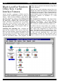
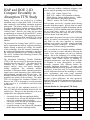
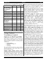
NEWS-II CARRIER SOFTWARE SYSTEMS Vol 14, No 2 SPRING, 1995 In This Issue: News: 1994/1995 E20-II Basic Training Schedules Extended...............................................................................2 3-1/2” Diskettes to Become Standard Issue for Software Updates..............................................................2 1995 Customer Survey Enclosed in Update Mailing ..................................................................................2 New Simulation Weather Data for Canada Released..................................................................................3 Block Load For Windows Offers New, Useful Interface Features...............................................................4 HAP / COMPLY 24 Translator Program Nears Release ............................................................................5 HAP and DOE 2.1D Compare Favorably in Absorption TTW Study ..........................................................6 Software: Using Outdoor Ventilation Control Options in HAP and SDL....................................................................7 Modeling Chiller Networks in HAP............................................................................................................8 Using the Unmet Load Printout to Diagnose Plant Simulation Problems...................................................9 Transferring Data from HAP v3.0 to v3.1................................................................................................11 Specifying Air System Multipliers in HAP................................................................................................11 Eight Programs Included In Spring Software Release Two E20-II programs and six Electronic Catalog programs were included in the first software mailing of 1995. In addition this release includes updated HAP simulation weather disks for three regions in North America. Summaries of program updates are provided below. E20-II Programs: • • • Hourly Analysis Program v3.12 - Corrects five bugs found in v3.10 since its release last November. System Design Load Program v1.12 - Corrects five bugs found in v1.10 since its release last November. HAP Simulation Weather Data: - Updates Canada, Northeast USA & Eastern Canada and Pacific USA & Western Canada weather data sets. For further details, please see the article on page 3. Electronic Catalog Programs: • • • • • • Reciprocating Chiller Selection v2.15 - Updates full load performance data for 30GT/GN190, part load performance data for 30GT/GN sizes 130, 150, 170, 190, 210; and permits input of water flow in gpm/ton. Rooftop Packaged Units v5.50 - Adds performance ratings for 50HX and 48/50SX units, updates performance data for five 48 and 50 series models, and deletes data for three obsolete models. Water Source Heat Pump Selection v2.20 - Provides updated selection and performance data for all currently available 50 series water source heat pumps. ACAPS v1.82 - Corrects several bugs which existed in ACAPS v1.80. Applied Acoustics Server v1.12 - Corrects one bug involving acoustic analysis for reciprocating chillers. Electronic Catalog Configuration Program v1.41 - Corrects one program bug. Program release sheets provide further information on each updated program. Customers will receive all the Electronic Catalog updates automatically. Only those customers who license the individual E20-II programs will receive these updates. ♦ Copyright 1995 Carrier Corporation Page 1 Printed on Recycled Paper Page 2 NEWS-II Spring, 1995 1994/1995 E20-II Basic Training Schedules Extended 3-1/2” Diskettes to Become Standard Issue for Software Updates Eight new dates were recently added to the 1994/1995 schedule of E20-II Basic Training Classes to extend the schedule through August. The E20-II Basic Training Classes provide in-depth, hands-on training for individual E20-II programs. They are intended for new E20-II users and existing users who want a refresher course. During 1995, Carrier Software Systems will be encouraging customers who are still receiving software on 5-1/4" disks to switch to 3-1/2" disks. We've found that many of our customers are not aware of the option to switch disk sizes for future update mailings at no charge, and have not taken advantage of this option even though 3-1/2" disks would serve their purposes better. Software on 3-1/2” disks can be installed if either the A: or B: drive in your computer handles 3-1/2” disks. Separate classes are being offered for HAP v3.1, Block Load v2.1 and Duct Design v3.2. The HAP session is a full day class with an enrollment fee of $150 per person. This fee includes lunch. The Block Load and Duct Design sessions are half day classes with an enrollment fee of $75 per person. For the Block Load and Duct Design classes, the fee does not include lunch. Dates for the additional classes are provided in the table below. Customers were sent schedule and registration information by direct mail during April. If you did not receive registration materials, please contact Carrier Software Systems at 315-432-6838. ♦ Schedule for Additional E20-II Basic Classes City HAP Block Load Duct Design Tampa, FL May 8 May 9 May 9 Richmond, VA May 16 May 17 May 17 Chicago, IL May 23 May 24 May 24 Honolulu, HI June 20 June 21 June 21 San Francisco, CA June 27 June 28 June 28 Detroit, MI May 25 - - Mobile, AL July 11 July 12 July 12 Cleveland, OH Aug 1 Aug 2 Aug 2 The Spring 1995 mailing of E20-II and Electronic Catalog software contains a prepaid postcard. If you wish to continue receiving software on 5-1/4" disks in future mailings, please sign and return the postcard. Any customer currently receiving 5-1/4" disks who does not return the postcard will be switched to 31/2" disks automatically. This change in disk sizes will take effect beginning with the Fall 1995 mailing of E20-II and Electronic Catalog software.♦ 1995 Customer Survey Enclosed in Update Mailing In addition to software, the Spring 1995 E20-II and Electronic Catalog software package you just received also includes a customer survey form. This form contains a variety of questions dealing with your use of computer software and hardware. Responses to the survey will help us tailor future software development plans to your needs as closely as possible. In addition to survey questions on these subjects, written comments, suggestions, requests and/or complaints are both welcomed and encouraged. Once you have completed the survey, please fold and tape it as indicated on the form and then mail it back to us. The survey form is postagepaid so there will be no cost to you. We strongly encourage customers to make use of this survey. It is an important means of setting future directions, identifying problems that need attention, and establishing communication that helps us determine how to deliver the highest quality products and service to you. ♦ Spring, 1995 NEWS-II New Simulation Weather Data for Canada Released The spring software mailing contains new HAP simulation weather data for Canadian cities. This material includes a new, expanded data set for Canada, and updates to Canadian data found on the Northeast USA & Eastern Canada data disks, and the Pacific USA & Western Canada data disks. The existing weather data set for “Canada and US Border Cities” contains typical meteorological year (TMY) weather data for 12 Canadian cities and 5 US cities located near the US/Canadian border. This data set is being replaced with new data for 41 Canadian cities. The new data was obtained from the Watsun Simulation Laboratory at the University of Waterloo. The Watsun Laboratory developed Canadian Weather for Energy Calculation (CWEC) data in work sponsored by the National Research Council of Canada. The CWEC data is typical meteorological year data derived from the Canadian Energy and Engineering Data Sets (CWEEDS) produced by Environment Canada. The new HAP simulation weather disks provide data for many of the unique climatic regions in Canada not covered by the original set of 12 Canadian cities, thereby improving the accuracy of energy simulations for these regions. Table 1. Canadian Cities In Weather Data Set Alberta Nova Scotia Calgary Sable Island Edmonton Shearwater (Halifax) Medicine Hat Ontario British Columbia London Abbotsford Muskoka Comox North Bay Fort St. John Ottawa Kamloops Sault Ste. Marie Prince George Thunder Bay Prince Rupert Toronto Sandspit Trenton Smithers Windsor Summerland Prince Edward Island Vancouver Charlottetown Victoria Quebec Manitoba Montreal Churchill Quebec Winnipeg Schefferville New Brunswick Saskatchewan Fredericton Estevan Saint John North Battleford Newfoundland Regina (TMY) Goose Bay Northwest Territories St. Johns Resolute Stephenville Yellowknife Yukon Territory Whitehorse Page 3 The new ”Canada (CWEC)” weather data set contains the cities listed in the table above. New CWEC data is provided for 41 of these cities; TMY data provided for Regina is the same as was provided on the previous “Canada & US Border Cities” data disk. In addition, TMY data for Buffalo, NY and International Falls, MN is provided for those applications in which the building site is closer to one of these US cities than the nearest CWEC site. On the new Northeast USA & Eastern Canada data disks, simulation weather data for the Canadian cities listed in Table 2 was updated with CWEC data. Table 2. Updated Cities on Northeast USA & Eastern Canada Data Disks New Brunswick Nova Scotia Fredericton Shearwater (Halifax) Newfoundland Prince Edward Island St. Johns Charlottetown Ontario Quebec Ottawa Montreal Toronto Quebec Finally, on the Pacific USA & Western Canada data disks, simulation weather data for the Canadian cities listed in Table 3 was updated with CWEC data. Note that TMY data for Regina, Saskatchewan is the same as provided on previous versions of the weather data disks. Table 3. Updated Cities on Pacific USA & Western Canada Data Disks Alberta Manitoba Edmonton Winnipeg British Columbia Vancouver The updated Canada weather data disks are being sent free of charge to all Canadian customers. Updated data disks are also being sent to those US customers who currently have the Canada, Northeast USA & Eastern Canada, or the Pacific USA & Western Canada data sets. The data is also available for purchase by any E20-II customer who does not currently have this data. ♦ Page 4 NEWS-II Block Load For Windows Offers New, Useful Interface Features Carrier unveiled a prototype of Block Load for Windows at the ASHRAE Exposition in Chicago in January. Block Load for Windows, which has not yet been released, is Carrier’s first Windows-based E20-II program. The prototype was on display for the many show attendees who visited the Carrier booth. Reaction to the program was very positive, with most viewers anxious for the arrival of the finished product. This article will describe some of the new, useful features of the program which you can expect to see soon. Something Old, Something New. Simplicity has been the key to Block Load’s success in the past. Block Load for Windows retains that simplicity and all of the basic load estimating capabilities of the DOS-based Block Load v2.1. Thus, anyone familiar with the DOS-based Block Load program can Spring, 1995 quickly learn to generate load estimates using Block Load for Windows. While the basic load estimating concepts have not changed, the whole look and feel of the Block Load interface has been revised with the implementation of a graphical user interface. This is where the real power of Block Load for Windows lies and is what significantly enhances its usefulness as a load estimating tool. The Graphical User Interface. The figure below contains a snapshot of the new Block Load for Windows user interface. As in most Windows applications, the program window contains a title bar, a menu bar, a tool bar and a main window area. For Block Load, the main window area contains a visual representation of all project data and shows how various data components are related to each other. This interface offers several advantages. First, many users find a visual representation of data easier to work with and understand than a text based representation. Second, all data associated with a project is shown at one time, rather than in bits and Spring, 1995 NEWS-II pieces as was the case in the DOS-based program. In this figure, the current city weather data is represented by the globe icon in the upper left portion of the main window area. In this example, the data is for Los Angeles. HVAC systems are represented by AHU icons along the upper center portion of the main window area. In this example there are three systems named “VAV Boxes”, “CAV System” and “CAV:VPAC”. Beneath each system icon are icons for the zones served by that system. The “VAV Boxes” system serves four zones named “North Wing”, “East Wing”, “South Wing” and “West Wing”. The other two HVAC systems serve one zone each. Finally, a separate work area is provided along the left side of the window area for zones which have not yet been attached to an HVAC system. In addition to the advantage of visualizing the data, the main window area can also be used to efficiently perform program tasks. For example, to edit system data, a user can double click on the desired HVAC system icon. A dialog box will automatically appear listing all inputs associated with that system. Or, to link a zone to a system, a user can click on the desired zone item and drag it to a location beneath one of the system icons. When the zone icon is “dropped” beneath a system icon, the program will automatically link the zone to that system and will draw lines connecting the two to indicate that they have been linked. The result of these features is that data can be manipulated and configured much faster than was possible with the menu-driven DOS-based program. Tool Bar Features. The Tool Bar, which runs along the top of the main window area, offers a number of additional features which can be used in conjunction with the main window area icons or by themselves to perform program tasks. For example, to print, edit or delete system data, a user first clicks on the desired system icon, and then presses the print, edit or delete button on the tool bar. On the other hand, to choose a new city or enter new zone or system data the appropriate tool bar button can be pressed to initiate each of these tasks. Menu Bar Features. Finally, the Menu Bar, which appears above the tool bar, provides features for manipulating program data using a conventional pulldown menu scheme. The File and Project Menus contain options for managing program data. City, Zone and System Menus provide options for working with city, zone and system data just as the Step One, Step Two and Step Three Menus did in the DOSbased Block Load Program. A Report Menu contains options for generating load calculation Page 5 outputs, and serves a function similar to the Step Four Menu in the DOS-based Block Load. Thus, the program’s user interface offers multiple ways to operate the program, and therefore allows the user to choose which is most efficient. Product Release. Readers will be happy to know that Block Load for Windows program development is nearing completion. By the time customers receive this newsletter, the program will be undergoing extensive beta testing to ensure a bug-free product is delivered. Beta testing is expected to be completed at the end of the second quarter. At that time the program will be mailed to all current Block Load v2.1 licensees. Others may license Block Load for Windows for a first year license fee of $495. The annual renewal fee is $100. ♦ HAP / COMPLY 24 Translator Program Nears Release The HAP / COMPLY 24 Translator Program, which has been discussed in previous issues of NEWS-II, has been completed and is in the final stages of testing. Testing was not finished in time to include the program in the Spring E20-II software mailing, but shipment of the software is anticipated in June. Current licensees of the HAP Title 24 package will receive the Translator Program free of charge. Final pricing for new licensees had not been determined at the time this newsletter went to press. The HAP / COMPLY 24 Translator Program is used to electronically transfer data from HAP to the COMPLY 24 program. COMPLY 24 , which is used to demonstrate compliance with the California Title 24 energy code, is developed and marketed by Gabel Dodd Associates of Berkeley, California. The HAP / COMPLY 24 data translation software serves as a labor saving tool for engineers using HAP to design systems and COMPLY 24 to perform compliance calculations. Readers in other parts of the country will be interested in these developments as California’s implementation of ASHRAE Standard 90.1 is being used as a model for DOE’s recommendation of a national implementation of the standard. Carrier is actively involved in work associated with implementation of the standard and in developing software in anticipation of a national standard. ♦ Page 6 NEWS-II Spring, 1995 HAP and DOE 2.1D Compare Favorably in Absorption TTW Study The following building simulation programs were used to analyze operating costs for the building: During 1994 Carrier was involved in a building simulation study in which HAP, DOE 2.1D and two other commonly used building simulation programs participated. The primary objective of the study was to support an absorption cooling technology transfer workshop being developed by the American Gas Cooling Center. However, the study also provided an opportunity to compare HAP and DOE 2.1 results for a controlled case study. This comparison showed close agreement between HAP and DOE 2.1D, which many engineers consider to be a benchmark in the industry. • The American Gas Cooling Center (AGCC) is a nonprofit organization that directly supports technology transfer relating to natural gas cooling. The transfer of this technology from the research community to the architect and engineering community is crucial to the successful marketing of gas cooling technology. The AGCC facilitates this technology transfer with educational programs. The Absorption Technology Transfer Workshop (TTW) is the first in a series of educational programs being developed by the AGCC. The objectives of the workshop are to enhance engineers’ ability to properly analyze, select and specify absorption cooling equipment. The workshop includes discussion of absorption chiller operating principles, capital costs, system integration, space requirements, and installation, operating and lifecycle costs. The building simulation study serves as the basis for the operating cost portion of the workshop. The initial TTW was developed for Southern California Gas. However, the TTW is designed so it can be presented in other areas as is, or modified to suit local needs and interests. The case study for this workshop involved a 12story, 323,000 sqft office building located in the Los Angeles area. Energy use and operating costs were compared for four equipment scenarios: • • • • A network of two 400-ton centrifugal chillers. A network of two 400-ton DF absorption chillers with a 10 F condenser delta-T at design. A network of two 400-ton DF absorption chillers with a 15 F condenser delta T at design. A hybrid network of one 400-ton DF absorption chiller and one 400-ton centrifugal chiller. • • • HAP v3.04. Author: Carrier Corp. DOE 2.1D. Author: US Department of Energy ESAS (Energy System Analysis Series). Author: Ross Meriwether/Consulting Engineering TRACE. Author: The Trane Company. Each program was run by a separate analyst having expertise with that program. Special effort was made to ensure each program modeled the building and the performance of the air handling and plant equipment on an equal basis, insofar as this was possible. Selected results from this study for DOE 2.1D and HAP are shown in the table below. On one hand, the general closeness of the HAP and DOE 2.1D results is not surprising. First, both HAP and DOE use the same approach to analyzing building heat transfer and loads: transfer functions and heat extraction techniques. In addition, both perform true 8760-hour energy simulations. Still, even with the use of similar modeling methods, there are reasons to expect differences between the results. First, each program was run by a different analyst. Due to the complexity of a building energy analysis, it is inevitable that different assumptions will be made about certain aspects of building or equipment performance, even when efforts are made to eliminate as many discrepancies as possible. Secondly, programs offer different features for modeling equipment performance. In some cases equipment modeling between programs could not be reconciled. In this case study, for example, there are specific differences between the modeling of cooling tower performance and water pump operation between HAP and DOE that could not be eliminated. In spite of these differences, the close agreement between HAP and DOE demonstrates that both use analytical methods at a similar level of sophistication and detail. ♦ Selected Results for Absorption TTW Study DOE 2.1 HAP Diff 3,958,430 4,061,898 +3% Two 400-Ton Centrifugals Total Bldg kWh/yr Electric OpCost, $/yr 466,718 486,407 +4% Bldg OpCost, $/yr 472,599 490,382 +4% Bldg Peak kW 1,302 1,449 +11% Spring, 1995 NEWS-II Selected Results for Absorption TTW (continued) DOE 2.1 HAP Diff Two 400-Ton DF Absorption Chillers, 15 F Condenser Delta-T Total Bldg kWh/yr 3,564,439 3,614,385 +1% Total Bldg Gas, MCF 9,439 10,155 +8% Electric OpCost, $/yr 399,157 404,768 +1% Bldg OpCost, $/yr 440,929 448,183 +2% 1,017 1,039 +2% 3,634,878 3,695,207 +2% Bldg Peak kW 400-Ton DF Absorp plus 400-Ton Centrifugal Total Bldg kWh/yr Total Bldg Gas, MCF 7,793 8,296 +6% Electric OpCost, $/yr 413,603 433,099 +5% Bldg OpCost, $/yr 448,148 468,970 +5% 1,142 1,241 +9% Bldg Peak kW Using Outdoor Ventilation Control Options in HAP and SDL When defining air handling systems in HAP and the System Design Load program, users can choose among four different options for controlling outdoor ventilation air: • • • • Constant Airflow Proportional to Supply Air Scheduled CO2 Sensor This article briefly describes these options and their intended applications. Each control option will be discussed separately below. Constant Airflow Control maintains outdoor ventilation at the design airflow rate for all occupied period hours and for unoccupied period hours when the ventilation dampers are open. For constant volume systems, constant ventilation airflow can be maintained without special controls and is the most Page 7 common control option used for CAV systems. For VAV systems, it is assumed special damper controls or booster fans are used to maintain a constant ventilation rate as the supply fan airflow varies. Note that this control also allows the user to specify whether ventilation dampers are open or closed during unoccupied periods. Thus, this control provides simple scheduling capabilities for eliminating ventilation airflow for unoccupied times. “Proportional to Supply Air” Control represents the use of uncontrolled or partially controlled ventilation airflow for VAV systems. With this option, ventilation airflow varies naturally as the supply airflow changes. Uncontrolled outdoor airflow tends to vary as a constant percentage of supply air. Thus, if the supply fan has throttled to 60% of its design value, ventilation air is 60% of its design value also. As with Constant Airflow control, the user has the opportunity to schedule the ventilation dampers open or closed during unoccupied period hours as necessary. CO2 Sensor Control provides a simple model for outdoor ventilation air control based on a CO2 sensor. Actual controls vary ventilation air to maintain indoor air quality based on measured C02 levels in the building. To model this control on a simple basis, the program assumes CO2 levels are directly related to the number of occupants in a zone. The program therefore varies ventilation airflow using a constant CFM/person value and the number of occupants in the building for the current hour. Scheduled Control is used when special controls are used to vary the outdoor ventilation airflow according to a predetermined time-clock schedule. For example, based on the time clock schedule, ventilation dampers might modulate to provide 1000 CFM of ventilation air from 6am to 9am, 1500 CFM from 9am to 12 noon, and 1250 CFM from 12 noon to 5pm. When this control option is used, the user specifies how ventilation air is varied by choosing one of the schedules stored in the program schedule database. This selection is made using an input on the last air system input screen, not the input screen on which ventilation airflow and controls are chosen. It is important to note that the “Scheduled Control” option should not be used simply as a means of eliminating ventilation air during unoccupied times. This can be done much more easily using the “Constant Airflow” and “Proportional To Supply Air” control options. Many users often overlook this and mistakenly use the “Scheduled Control” option when “Constant Airflow” or “Proportional to Supply Air” would be a more appropriate selection. ♦ Page 8 NEWS-II Modeling Chiller Networks in HAP HAP offers useful features for studying the performance of chiller networks. This article explains how to simulate chiller networks, and discusses some of the nuances of network modeling. Entering Data. Entering data for a chiller network plant differs from other types of plant equipment. For a heat pump or a rooftop unit for example, data describing the equipment is simply entered and stored. For a chiller network, however, data must be entered in two stages. First, data describing the individual chillers is entered and stored. Second, data describing the network is entered and stored. To illustrate this procedure, consider a network containing one 300-ton centrifugal chiller and one 400-ton centrifugal chiller. To enter data for this network, the following steps must be used: 1. Enter and store data describing each chiller as a individual plant. Thus, two plants would be entered. One describes the 300-ton chiller, and one defines the 400-ton chiller. 2. Enter and store data for a third plant. On the first plant input screen specify the classification as “cooling” and the type as “chiller network”. On the second input screen, specify the air systems the chiller network serves. On the third input screen define the number of chillers in the network (2 in our example). Then specify the chillers linked together to form the network. This is done using a pop-up list of the individual chillers already stored in the HAP plant database. Thus, for our example, the 300-ton centrifugal and the 400-ton centrifugal entered in step 1 would be selected from the database list to link them to the network. This input screen also allows the control for the network to be defined as sequenced (i.e., lead/lag) or non-sequenced. When sequenced operation is used, the order in which chillers in the network are turned on and off can be defined. Simulating Network Operation. Running plant and building simulations for a chiller network is simple except for the issue of plant selection: 1. To simulate the chiller network plant, choose the simulate option on the Plant Menu. Then choose the chiller network plant on the plant selection list. Do not choose the individual chillers connected to the network. When a chiller network is selected for simulation, the program Spring, 1995 will automatically use the input data for the network and the individual chillers connected to the network to simulate network operation. 2. When entering building data, you’re asked to specify the plants included in the building so the. program can determine which plant energy consumption data should be used in building cost calculations. Further, by examining the list of systems served by that plant, the program is also able to determine which air system energy consumption data to use in cost calculations. All of this information is associated with the chiller network plant, not the individual chillers connected to the plant. Thus, the chiller network plant must be included in the building, but the individual chillers must not be included. Flexible Features. The features for analyzing chiller networks in HAP provide a high degree of flexibility. Chillers of any type and cooling capacity can be connected together. For example, a simple network might consist of two identical 200-ton chillers. A complex network might contain one 250-ton gas engine driven chiller for peak demand shaving as the lag chiller, and a 250-ton electric screw chiller and 350-ton centrifugal chiller as the lead chillers. HAP provides features for easily modeling both simple and complex arrangements such as these. A Useful Shortcut. When working with a simple network which contains two or more identical chillers, it is not necessary to enter and store data for each individual chiller separately. For example, suppose a network consists of three identical 150-ton chillers. Instead of entering and storing the same individual chiller data three times, the chiller data can be entered once. When defining the network, simply connect the same chiller to the network three times. This reduces the input effort by two thirds. Nuances. One common point of confusion about network modeling involves the use of individual chiller data in a network simulation. Because data is entered in two stages, certain input items for the chiller network plant supersede data entered for the individual chillers: • • • Specification of air systems served by the plant. Chiller water reset specifications. Specifications for direct and indirect free cooling for the individual chiller are currently not able to be used in chiller network simulations. For further information on modeling chiller networks, please refer to the Energy Analysis User’s Manual for HAP, pages 3-7 and 12-15 thru 12-17. ♦ Spring, 1995 NEWS-II Using the Unmet Load Printout to Diagnose Plant Simulation Problems While simulating the operation of plant equipment in HAP, the program continually checks plant capacity against the hourly cooling or heating demand. When demand exceeds the plant capacity, the program reports an “unmet load” condition. This article describes common causes for unmet plant loads, and discusses how to diagnose and correct these simulation problems. Report Format. When unmet loads occur, the program reports these conditions on a printout similar to the one shown below. This sample is for a 120-ton chiller and contains one table of cooling statistics. Depending on the type of equipment being simulated, separate tables for cooling and/or heating will be provided. For a heat pump for example, tables for cooling, heating and auxiliary heating statistics will be provided. Each table in this report provides a month-by-month account of the equipment performance. Separate columns list the number of hours the plant could and could not meet loads. Statistics describing the amount by which loads exceed equipment capacity are also provided. Page 9 demand is between 120 and 126 tons. For 2 hours the chiller is deficient by 5 to 10% (i.e. the demand is between 126 and 132 tons), and for 2 hours the chiller is deficient by more than 10% (i.e., the demand is above 132 tons). Causes. Unmet load conditions result from one of the two causes listed below. Each will be discussed further in the application sections of this article. • • A plant load exceeds the plant capacity. A load exists, but the plant has been turned off. Applications - Constant Capacity. Certain plant models in HAP assume constant capacity over the range of operating conditions experienced. Heating plants and computer-generated chiller models are examples of models assuming constant capacity. For example, if a chiller has a 120-ton capacity, any cooling demands larger than 120 tons will result in an unmet load condition. When this type of problem occurs, the largest number of unmet loads will occur in peak cooling months for cooling equipment and peak heating months for heating equipment. The number of unmet load hours will decrease in intermediate and off-peak months. When evaluating this problem, first consider the number of unmet load conditions. If relatively few unmet load hours exist and all are conditions in which the equipment is deficient by small amounts, the problem may not require modification of the plant In the sample below, for the month of May the chiller capacity. If the equipment capacity was set equal to is able to meet cooling demands for 733 hours. For the “estimated maximum plant load”, it is sized for 11 hours, the cooling demand exceeds the chiller’s the design day criteria used in the design portion of 120-ton capacity. For 7 of these hours, the chiller is HAP (i.e., 1% or 2.5% design). Thus it is not deficient by less than 5%. That is, the cooling unusual for more extreme conditions to exist for a limited number of hours per year. In many cases, engineers PLANT SIMULATION UNMET LOAD REPORT accept these unmet load Plant: Chiller Plant 03-17-95 conditions. ************************************************************************* TABLE 1. COOLING PLANT STATISTICS ------------------------------------------------------------------------Plant Capacity --- Plant Capacity Insufficient to Meet Load ---Is Sufficient By 0%-5% By 5%-10% By > 10% Total Month (hr/month) (hr/month) (hr/month) (hr/month) (hr/month) ------------------------------------------------------------------------Jan 240 0 0 0 0 Feb 288 0 0 0 0 Mar 607 0 0 0 0 Apr 720 0 0 0 0 May 733 7 2 2 11 June 645 22 24 29 75 July 634 39 35 36 110 Aug 654 36 29 25 90 Sept 715 4 1 0 5 Oct 744 0 0 0 0 Nov 649 0 0 0 0 Dec 257 0 0 0 0 ------------------------------------------------------------------------Totals 6886 108 91 92 291 ------------------------------------------------------------------------- However, if a large number of unmet loads exist, or the size of the deficiency is large, it may indicate a problem with equipment modeling. Further, it will usually have adverse effects on comparisons between alternative equipment types, especially if one plant alternative has unmet loads and another doesn’t. To correct such a problem, first use the “generate simulation output” option on the Plant (continued on page 10) Page 10 NEWS-II Unmet Plant Loads (continued from page 9) Menu to review displays of hourly results for the month when the largest number of unmet loads occur to determine the maximum plant load. Then adjust the plant capacity to meet this load and rerun the plant simulation. A shortcut approach which is simpler but more approximate is to increase equipment capacity by the amount the Unmet Load Report indicates the equipment is deficient. For example, if the Unmet Load Report indicates that in the worst case the plant is deficient by 5 to 10%, increasing the plant capacity by 10% should solve the problem. The only drawback to this approach is that without checking hourly results, you cannot tell whether the maximum deficiency is 5.1% or 10%. Thus, this shortcut approach can result in the plant being oversized. Applications - Variable Capacity. Other plant models in HAP consider the variation in equipment capacity as operating conditions change. Examples include the computer-generated models for all DX cooling units and heat pumps, and the computergenerated model for water-cooled reciprocating chillers. In addition, capacity variation is an option in all user-defined plant models. For example, the computer-generated model for a packaged rooftop cooling unit uses a correlation between cooling capacity and outdoor temperature. Documentation for this correlation is provided in Chapter 12 of the Energy Analysis User’s Manual for HAP. As the graph below shows, a unit with a 10-ton capacity at 95 F outdoor air, has approximately 11 tons of capacity at 75 F outdoor air, and approximately 9 tons of capacity at 115 F outdoor air. Figure 12.1 from Energy Analysis User’s Manual Spring, 1995 Because capacity varies as a function of outdoor temperature (or other conditions) for these models, diagnosing unmet loads becomes more difficult. For example, if a DX cooling unit is defined with a 10ton capacity at 95 F outdoor air, and a 10-ton load occurs at 100 F outdoor air, an unmet load condition will occur because the unit capacity drops below 10 tons at temperatures warmer than the 95 F. To determine how to correct these problems, first determine the size and time of large loads using the graph and display options for plant simulation results which were described earlier in this article. Second, determine the operating conditions for the specific hour when these large loads occur. For a DX cooling unit, for example, the outdoor air temperature for these hours would be determined from simulation weather printouts. Finally, this data should be used in conjunction with the equipment performance graphs in Chapter 12 of the Energy Analysis User’s Manual to determine what conditions cause unmet loads and how much plant capacity should be increased to resolve these problems. For user-defined plant models a similar approach would be employed using load data, the corresponding operating conditions and user-defined capacity data to determine how to correct the problem. Applications - Equipment Cutoff. Finally, for DX cooling equipment and for air source heat pumps, equipment cutoff points are defined below which the equipment is not permitted to operate. For example, if an air system cooling coil load exists for an outdoor temperature below the cooling equipment cutoff temperature, the DX unit will not be able to operate and an unmet load condition will result. For cooling equipment the symptom of this problem is unmet load conditions in cool months of the year with all such unmet loads reported as deficient by more than 10% (i.e., the equipment has been disabled so it has zero capacity and is therefore more than 10% deficient versus any load that occurs). The solution to this problem is to permit the cooling equipment to operate at colder outdoor temperatures either by lowering the cutoff temperature or by adding low temperature operating controls such as head pressure control. For air source heat pumps a similar problem occurs if heating loads occur below the outdoor air cutoff temperature and no auxiliary heating exists. These unmet loads appear in peak heating months as conditions with capacity deficient by more than 10%. In this case, the solution is to lower the cutoff temperature or add an auxiliary heating unit. ♦ Spring, 1995 NEWS-II Page 11 Transferring Data from HAP v3.0 to v3.1 Specifying Air System Multipliers in HAP Q. I started a project last fall using HAP v3.04. Now that we have HAP v3.1, I’d like to move the data to v3.1 to take advantage of its expanded calculation and output features. How can I do this? Q. I am using HAP to run an energy analysis for a building which contains a 42-zone VAV/RH system. Each zone VAV box contains an electric reheat coil. When I define the electric resistance heating plant, HAP asks me to specify the coils in the air system served by electric heat. I do this by entering values on the “Air System Selection Screen”. When I do this, should I specify a 42 in the terminal heating column to account for the reheat coils in all 42 zones? Or should I simply specify 1 as the quantity and assume the program will use electric heat for all 42 zone reheat coils? A. Option 5 (“Retrieve Program Data From Previous Version”) on the HAP v3.1 Data Management Menu can be used to convert HAP v3.0 data for use with v3.1. Use the following procedure to retrieve this data: 1. Make sure the HAP v3.0 data you wish to retrieve is stored on the hard disk. Data cannot be directly retrieved from a v3.0 floppy archive disk. It must be retrieved from a HAP v3.0 user data directory on the hard disk. 2. Run HAP v3.1 and create a data subdirectory whose name matches the HAP v3.0 subdirectory containing the data you want to retrieve. For example, if the HAP v3.0 data is stored in a subdirectory named JOB104, the current data subdirectory in HAP v3.1 must also be named JOB104. A. You should specify a quantity of 1. Do not specify 42. When specifying which heating coils in an air system are served by heating equipment, assignments are made on a system-wide basis. Thus, if you specify a quantity of 1 for terminal reheat coils, the program will automatically use that heating equipment for the terminal reheat coils for all zones in the system. ♦ 3. Finally, choose option 5 (“Retrieve Program Data From Previous Version”) on the HAP v3.1 Data Management Menu. Data files will be copied from the HAP v3.0 data subdirectory to the v3.1 subdirectory and will be converted to a format compatible with HAP v3.1. The data transfer retrieves 100% of the HAP v3.0 data. The same retrieval features are offered for the System Design Load Program v1.1. For further information, please refer to the Update Bulletin for HAP v3.1 and SDL v1.1. This bulletin was distributed with HAP v3.1 and System Design Load v1.1 when these programs were released last fall. ♦ HAP v3.1 Data Management Menu The Air System Selection Screen HAP Plant Input Page 12 Program Name NEWS-II Spring, 1995 Version 1st Year Number License Fee Annual Renewal Fee Disk Space Disk Space for Program for Data (kB) (kB) Note 1.10 2.11 2.12 1.00 3.24 2.14 1.40 2.10 3.12 1.12 3.00 2.00 2.01 1.12 1.10 3.03 $295 $350 $495 $195 $295 $595 NA $95 $1195 $150 $95 $250 $250 $795 $95 $150 $60 $35 $100 $40 $60 $60 NA $20 $240 $10 $10 $10 $10 $160 $10 $15 2,000 356 654 646 1,260 2,560 1,200 380 4,200 154 66 352 256 2,300 64 860 min 2 36 326 236 min 200 min 348 0 50 min 126 0 0 204 82 min 126 18 min 385 H H H H H H H H H,M H H H H H,M H H 1.82 1.12 1.12 2.30 1.41 2.15 5.50 2.10 2.20 2.01 NC NC NC NC NC NC NC NC NC NC NC NC NC NC NC NC NC NC NC NC 3,384 2,500 450 218 1,100 1,370 1,608 582 774 688 504 0 min 2 0 0 30 min 2 0 0 0 H,M H H H H H,M H H H H E20-II Programs: Applied Acoustics Bin Operating Cost Analysis Block Load Block Load Lite Duct Design DuctLINK E20-II Configuration Engr. Economic Analysis Hourly Analysis Program (HAP) PsychGRAPH Refrigerant Piping Sheet Metal & Eqpt Estimating Sheet Metal Layout System Design Load Program U-Value Calculator Water Piping Design E-CAT Programs: ACAPS Acoustics Server Air Terminal Selection Commercial Split Systems Selection Electronic Catalog Configuration Reciprocating Chiller Selection Rooftop Packaged Units Selection Vertical Packaged Units Selection Water Source Heat Pump Selection 42 Series Fan Coil Selection Key: H=Hard Disk Required. M=Math Coprocessor Recommended NC=No Charge. NA=Not Applicable. Software Support Software Correspondence E20-II customers are provided with free, unlimited software support as part of the software license. Software support is provided through your local Carrier distributor or sales office, the Carrier Regional Software Managers (RSMs) and the Syracuse software support staff. To obtain software assistance from an RSM or from Syracuse, simply call our toll-free support line listed below. For information about software licenses, renewals, mailings and changes of address please contact: Toll-Free Support Line: 1-800-253-1794 Carrier Corporation Software Systems Network TR-1 Room 250 P.O. Box 4808 Syracuse, New York, 13221 Attn: Joanne Sherwood Phone: 315-432-7072. FAX: 315-432-6844