Download Content-based Projections for Panoramic Images and - PUC-Rio

INSTITUTO NACIONAL DE MATEMÁTICA PURA E APLICADA
Content-based Projections for
Panoramic Images and Videos
Leonardo Koller Sacht
Advisor: Paulo Cezar Carvalho
Co-advisor: Luiz Velho
Rio de Janeiro, April 5, 2010.
Master thesis committee:
Paulo Cezar Pinto Carvalho (advisor) - IMPA
Luiz Carlos Pacheco Rodrigues Velho (co-advisor) - IMPA
Marcelo Gattass - PUC-Rio
Luiz Henrique de Figueiredo (substitute) - IMPA
Acknowledgements
First of all, I would like to thank my mother for always supporting me, encouraging
me and pushing me forward.
I would like to thank Professor Paulo Cezar Carvalho for guiding my studies during
the last years and for giving valuable suggestions and contributions to this work.
I am grateful to Professor Luiz Velho for receiving me very well in the Visgraf Laboratory, for introducing me to the theme of this thesis, for giving great ideas for the
development of this work and for providing key discussions about the theme.
I would also like to thank Professor Marcelo Gattass for helping me on the Computer
Vision aspects of this work.
A more general acknowledgement to all Professors from IMPA and UFSC that contributed to my academic growth.
I want to thank all my colleagues from the Visgraf Lab that somehow helped me in this
thesis: Thiago Pereira, Adriana Schulz, Djalma Lucio, Gabriel Duarte, Marcelo Cicconet,
Francisco Ganacim and Leandro Cruz. Also, I want to thank all friends at IMPA for
making the years of my masters studies not only constructive but also very pleasant.
I would like to thank all the people that work at IMPA and contribute to keeping it
a place of excellence to study Mathematics.
I am very grateful to the Brazilian Government for giving me conditions to focus on
my studies and CNPq for the financial support.
Resumo
Câmeras comuns geralmente capturam um campo de visão bastante limitado, por
volta de noventa graus. A razão para este fato é que quando o campo de visão se torna
maior, a projeção que estas câmeras usam começa a introduzir distorções não-naturais e
não-triviais. Esta dissertação estuda estas distorções com a finalidade de obter imagens
panorâmicas, isto é, imagens de grandes campos de visão.
Após modelar o campo de visão como uma esfera unitária, o problema passa a ser
achar uma projeção de um subconjunto da esfera unitária em um plano de imagem, com
propriedades desejáveis. Nós fazemos uma discussão aprofundada de Carroll et. al ([1]),
no qual preservação de linhas retas e formas de objetos são colocados como as propiedades
desejáveis principais e uma solução de otimização é proposta. A seguir, nós mostramos
imagens panorâmicas obtidas por este método e concluı́mos que ele funciona bem numa
variedade de cenas.
Esta dissertação também faz um estudo inovador sobre vı́deos panorâmicos, isto é,
vı́deos nos quais cada quadro é construı́do a partir de um grande campo de visão. Nós introduzimos um modelo matemático para o problema, discutimos propriedades de coerência
temporal desejáveis, formulamos equações que representam estas propriedades, propomos
uma solução de otimização para um caso particular e apontamos direções futuras.
Palavras-chave: Esfera visı́vel, imagens panorâmicas, vı́deos panorâmicos.
Abstract
Common cameras usually capture a very narrow field of view (FOV), around ninety
degrees. The reason for this fact is that when the field of view becomes wider, the
projection that these cameras use starts introducing unnatural and nontrivial distortions.
This thesis studies these distortions in order to obtain panoramic images, i.e., images of
wide fields of view.
After modeling the FOV as a unit sphere, the problem becomes finding a projection
from a subset of the unit sphere to the image plane, with desirable properties. We provide
an in-depth discussion of Carroll et. al ([1]), where preservation of straight lines and
object shapes are stated as the main desirable properties and an optimization solution is
proposed. Next, we show panoramic images obtained by this method and conclude that
it works well in a variety of scenes.
This thesis also provides a novel study about panoramic videos, i.e., videos where each
frame is constructed from a wide FOV. We introduce a mathematical model for this problem, discuss desirable temporal coherence properties, formulate equations that represent
this properties, propose an optimization solution for a particular case and point future
directions.
Keywords: Viewing sphere, panoramic images, panoramic videos.
Contents
Introduction
1
Motivation and Overview of the Problem . . . . . . . . . . . . . . . . . . . . . .
1
Goals
. . . . . . . . . . . . . . . . . . . . . . . . . . . . . . . . . . . . . . . . .
3
Original Contributions . . . . . . . . . . . . . . . . . . . . . . . . . . . . . . . .
3
Structure of the thesis: a time line . . . . . . . . . . . . . . . . . . . . . . . . .
4
1 Panoramic images
6
1.1
The Viewing Sphere . . . . . . . . . . . . . . . . . . . . . . . . . . . . . .
1.2
Problem Statement . . . . . . . . . . . . . . . . . . . . . . . . . . . . . . . 10
1.3
Standard Projections . . . . . . . . . . . . . . . . . . . . . . . . . . . . . . 10
1.4
1.5
6
1.3.1
Perspective Projection . . . . . . . . . . . . . . . . . . . . . . . . . 10
1.3.2
Stereographic Projection . . . . . . . . . . . . . . . . . . . . . . . . 13
1.3.3
Mercator Projection . . . . . . . . . . . . . . . . . . . . . . . . . . 14
Modified Standard Projections . . . . . . . . . . . . . . . . . . . . . . . . . 15
1.4.1
Perspereographic Projections
. . . . . . . . . . . . . . . . . . . . . 16
1.4.2
Perspective Projection Centered on Other Points . . . . . . . . . . 18
1.4.3
Recti-Perspective Projection . . . . . . . . . . . . . . . . . . . . . . 19
Previous Approaches . . . . . . . . . . . . . . . . . . . . . . . . . . . . . . 20
1.5.1
Correction of Geometric Perceptual Distortions in Pictures . . . . . 21
1.5.2
Artistic Multiprojection Rendering . . . . . . . . . . . . . . . . . . 23
1.5.3
Squaring the Circle in Panoramas . . . . . . . . . . . . . . . . . . . 25
1.5.4
Other Approaches . . . . . . . . . . . . . . . . . . . . . . . . . . . . 27
2 Optimizing Content-Preserving Projections for Wide-Angle Images
28
2.1
Desirable Properties . . . . . . . . . . . . . . . . . . . . . . . . . . . . . . 29
2.2
User Interface . . . . . . . . . . . . . . . . . . . . . . . . . . . . . . . . . . 31
2.3
Discretization of the Viewing Sphere . . . . . . . . . . . . . . . . . . . . . 35
2.4
Conformality . . . . . . . . . . . . . . . . . . . . . . . . . . . . . . . . . . 36
2.5
2.4.1
Differential Geometry and the Cauchy-Riemann Equations . . . . . 36
2.4.2
Examples . . . . . . . . . . . . . . . . . . . . . . . . . . . . . . . . 40
2.4.3
Energy Term . . . . . . . . . . . . . . . . . . . . . . . . . . . . . . 42
Straight Lines . . . . . . . . . . . . . . . . . . . . . . . . . . . . . . . . . . 44
5
2.6
2.5.1
Energy terms . . . . . . . . . . . . . . . . . . . . . . . . . . . . . . 48
2.5.2
Inverting Bilinear Interpolation . . . . . . . . . . . . . . . . . . . . 52
Smoothness . . . . . . . . . . . . . . . . . . . . . . . . . . . . . . . . . . . 56
2.6.1
Energy Term . . . . . . . . . . . . . . . . . . . . . . . . . . . . . . 57
2.7
Spatially-Varying Weighting . . . . . . . . . . . . . . . . . . . . . . . . . . 58
2.8
Minimization . . . . . . . . . . . . . . . . . . . . . . . . . . . . . . . . . . 62
2.8.1
Total Energy . . . . . . . . . . . . . . . . . . . . . . . . . . . . . . 63
2.8.2
Eigenvalue/Eigenvector Method . . . . . . . . . . . . . . . . . . . . 63
2.8.3
Linear System Method . . . . . . . . . . . . . . . . . . . . . . . . . 65
2.8.4
Results in each iteration . . . . . . . . . . . . . . . . . . . . . . . . 68
3 Results
73
3.1
Result 1 . . . . . . . . . . . . . . . . . . . . . . . . . . . . . . . . . . . . . 74
3.2
Result 2 . . . . . . . . . . . . . . . . . . . . . . . . . . . . . . . . . . . . . 78
3.3
Result 3 . . . . . . . . . . . . . . . . . . . . . . . . . . . . . . . . . . . . . 82
3.4
Result 4 . . . . . . . . . . . . . . . . . . . . . . . . . . . . . . . . . . . . . 86
3.5
Result 5 . . . . . . . . . . . . . . . . . . . . . . . . . . . . . . . . . . . . . 90
3.6
Failure cases . . . . . . . . . . . . . . . . . . . . . . . . . . . . . . . . . . . 92
3.7
Result Discussion . . . . . . . . . . . . . . . . . . . . . . . . . . . . . . . . 94
4 Panoramic Videos
97
4.1
Overview . . . . . . . . . . . . . . . . . . . . . . . . . . . . . . . . . . . . . 97
4.2
The three cases . . . . . . . . . . . . . . . . . . . . . . . . . . . . . . . . . 98
4.3
Desirable Properties . . . . . . . . . . . . . . . . . . . . . . . . . . . . . . 98
4.4
The Temporal Viewing Sphere and Problem Statement . . . . . . . . . . . 100
4.5
Transition Functions . . . . . . . . . . . . . . . . . . . . . . . . . . . . . . 102
4.6
Case 1 - Stationary VP, Stationary FOV and Moving Objects . . . . . . . 104
4.7
4.8
4.6.1
Temporal Coherence Equations . . . . . . . . . . . . . . . . . . . . 104
4.6.2
Discretization of the temporal viewing sphere . . . . . . . . . . . . 106
4.6.3
Total energy, minimization and results . . . . . . . . . . . . . . . . 107
4.6.4
Implementation Details . . . . . . . . . . . . . . . . . . . . . . . . . 113
4.6.5
Other Solutions . . . . . . . . . . . . . . . . . . . . . . . . . . . . . 115
Case 2 - Stationary VP, Moving FOV and Stationary Objects . . . . . . . 115
4.7.1
Temporal Coherence Equations . . . . . . . . . . . . . . . . . . . . 115
4.7.2
A solution . . . . . . . . . . . . . . . . . . . . . . . . . . . . . . . . 116
Concluding Remarks . . . . . . . . . . . . . . . . . . . . . . . . . . . . . . 116
A Application Software
118
A.1 Application and user’s manual . . . . . . . . . . . . . . . . . . . . . . . . . 118
A.2 Implementation Details . . . . . . . . . . . . . . . . . . . . . . . . . . . . . 122
A.2.1 Window 1 . . . . . . . . . . . . . . . . . . . . . . . . . . . . . . . . 123
6
A.2.2 Window 2 . . . . . . . . . . . . . . . . . . . . . . . . . . . . . . . . 124
A.2.3 Matlab processing . . . . . . . . . . . . . . . . . . . . . . . . . . . . 125
B Feature Detection in Equirectangular Images
128
B.1 Automatic Face Detection in Equirectangular
Images . . . . . . . . . . . . . . . . . . . . . . . . . . . . . . . . . . . . . . 128
B.1.1 Robust Real-time Face Detection . . . . . . . . . . . . . . . . . . . 129
B.1.2 Method and Implementation . . . . . . . . . . . . . . . . . . . . . . 133
B.1.3 Results . . . . . . . . . . . . . . . . . . . . . . . . . . . . . . . . . . 135
B.1.4 Weight Field
. . . . . . . . . . . . . . . . . . . . . . . . . . . . . . 136
B.2 Semiautomatic Line Detection in Equirectangular Images . . . . . . . . . . 137
B.2.1 The Hough Transform . . . . . . . . . . . . . . . . . . . . . . . . . 137
B.2.2 Bilateral Filter . . . . . . . . . . . . . . . . . . . . . . . . . . . . . 140
B.2.3 Eigenvalue Processing . . . . . . . . . . . . . . . . . . . . . . . . . 141
B.2.4 The Method . . . . . . . . . . . . . . . . . . . . . . . . . . . . . . . 143
B.2.5 Results . . . . . . . . . . . . . . . . . . . . . . . . . . . . . . . . . . 148
B.2.6 Concluding remarks . . . . . . . . . . . . . . . . . . . . . . . . . . . 149
Conclusion
151
Review . . . . . . . . . . . . . . . . . . . . . . . . . . . . . . . . . . . . . . . . . 151
Discussion . . . . . . . . . . . . . . . . . . . . . . . . . . . . . . . . . . . . . . . 152
Future Work
. . . . . . . . . . . . . . . . . . . . . . . . . . . . . . . . . . . . . 153
Bibliography
155
i
Introduction
Motivation and Overview of the Problem
This thesis studies the problem of obtaining perceptually acceptable panoramic images,
which are images that represents wide fields of view.
One of the motivations for this problem is that common cameras capture just a limited
field of view (FOV), usually near 90 degree longitude and 90 degree longitude, while our
eyes see about 150 degree longitude and 120 degree latitude. When we see a photograph,
it is as if we were seeing the world through a limited window. This limitation in common
photographs happens because they are produced under a projection that approximates
the perspective projection, which stretches objects too much for wide FOVs.
The panoramic images can be used to extrapolate our perception, since they can
capture FOVs beyond the human eye. Also, a panoramic image allows us to better
represent an entire scene. There may be important parts in a scene that could not be
seen under a limited FOV.
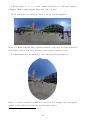
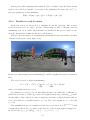
The study of this topic became possible only recently with the development of stitching
software and equipment ([2], [3] and [4]). With these techniques, it is possible to create
an image of the entire viewing sphere centered at the viewpoint, an image that contains
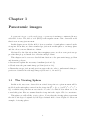
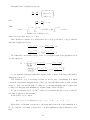
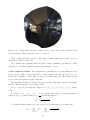
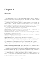
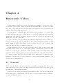
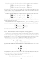
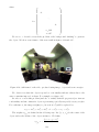
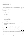
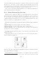
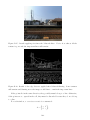
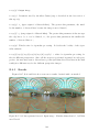
the visual information that is seen from this viewpoint in all possible directions. In figure
1 one can see an example of such image, which we call equirectangular image.
Once we have an image that represents the viewing sphere, what is left to be done
is to find a projection from the sphere to the plane that results in a perceptually good
result. Some previous works as [5], [6], [7], [4] and [8] considered this problem. The main
difficulty that arises is to satisfy two important perceptual properties: preservation of
shapes, i.e., objects in the scene should not appear too stretched in the final panoramic
image, and preservation of straight lines, i.e., straight lines the scene should be mapped
to straight lines in the final panoramic image.
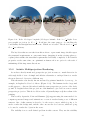
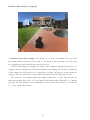
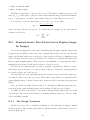
The paper studied in depth in this thesis, named Optimizing content-preserving projections for wide-angle images ([1]), addresses these two properties by formulating energies
that measure how a projection distorts shapes and bends lines. The user marks in an
interface the lines she wants to be preserved and the method detect regions where the
projection should preserve more shapes, as face regions for example. Based on this in-
1
Figure 1: Example of equirectangular image.
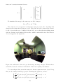
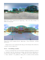
formation, the method formulates the energies and the minimizer of a weighted sum of
these energies is the panoramic image that most satisfy these properties. An extra term
for modeling the smoothness of the projection is necessary to avoid mappings that vary
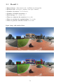
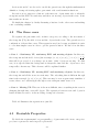
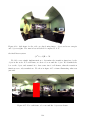
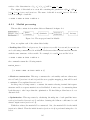
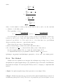
too much to satisfy the constrains. An example of panoramic image produced by this
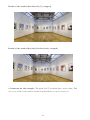
method is shown in figure 2.
Figure 2: Example of result produced by the method deeply discussed in this thesis.
This thesis is also concerned about the problem of obtaining perceptually acceptable
panoramic videos. This theme has the motivations we already mentioned for panoramic
images, but also it has more interesting practical applications. The development of ideas
in this field could lead to new ways of filming, which could be applicable for cinema and
sport broadcasting, for example.
2
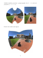
Recently, capture devices that film a wide field of view were invented. An example of it
can be found in [9]. These cameras return a video where each frame is an equirectangular
image for the respective time. Again, what is left to be done is to project this set of
viewing spheres (which we call temporal viewing sphere) to a set of images.
Very little work has been done on this subject. The strategy adopted in this thesis is
to adapt the theory studied for images and include new desirable properties that model
temporal coherence, in order to produce a perceptually good panoramic video.
Goals
This thesis has the following goals:
• Study and understand the panoramic image problem: In our work, we do a
review of the methods proposed up to the moment, which is necessary to understand the
difficulties and challenges of the problem.
• Deeply detail one reference on this topic: After doing the review, we elected
[1] as the main reference of this thesis because it satisfies most of the properties we state
as desirable. All the details, even the ones that were omitted in the reference, are explained in this thesis.
• Propose extensions for this reference: Beyond detailing [1], we propose two extensions for it: feature detection on equirectangular images and panoramic videos.
• Focus on mathematical aspects of the problem: All the mathematical techniques related to the problem are discussed in details in this thesis. Perceptual aspects
are also discussed and implementation aspects are left as appendix.
Original Contributions
We believe that the two most important contributions of our work are:
• Statement, modeling and solutions for the panoramic video problem: As
far as we know, this thesis is the first work where the problem of obtaining a video where
each frame represents a wide FOV is considered. We consider desirable properties for
this problem, that depend on temporal coherence of the objects and of the entire scene,
we model the problem as the one of finding a projection and we propose an optimization
solution for a particular case. These contributions are all found in chapter 4.
3
• An in-depth conclusive analysis of [1]: As we already mentioned, [1] omits details of their method. This thesis makes a complete mathematical analysis of their work,
and also a conclusive analysis based on the results produced by their method. This analysis is in chapters 2 and 3.
Our work has other contributions of less impact, but also important in the context of
this thesis:
• Line detection on equirectangular images: We propose a method to semiautomatically detect straight lines of the world in equirectangular images. This detection
was pointed as future work in [1] and helps the user in the task of marking lines. This
contribution can be found in appendix B.
• Application software: We propose in this work an application software that has
some features that the interface proposed in [1] does not have, such as specification of
FOV, vertices and number of iteration. This application is explained in appendix A.
• Perspereographic Projections: We developed a set of projections that interpolates
conformality and preservation of straight lines in a very intuitive way. It has the same
purpose of the projection presented in [5], but is obtained in a much easier way. These
projections are in section 1.4.1.
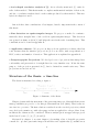
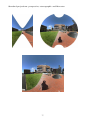
Structure of the thesis: a time line
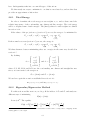
The thesis is structured according to figure 3.
Figure 3: Structure of the thesis.
Chapter 1 starts with the statement of the panoramic image problem and then reviews
many possibilities proposed to solve this problem until last year (2009). That is why we
associate it to past time. The first solutions considered are the standard projections, which
were developed centuries ago with other purposes but are applicable to the problem. Some
modifications of them are also considered. Then we analyze previous approaches proposed
in the last 15 years: [5], [6], [7], [4] and [8].
Motivated by chapter 1, we start chapter 2 by making a list of desirable properties
a method to produce panoramic images should have and explain why [1] satisfies most
4
of them. Since [1] is very recent (it was published in SIGGRAPH 2009) we associate it
to present time. Each section of this reference is discussed and theoretical details are
rigorously posed.
In chapter 3, we show the results produced by the method. Good results are shown,
each one illustrating some interesting feature of the method. Also, some failure cases are
discussed.
In order to complement the discussion about [1], we provide two appendices. In
appendix A, we show the application software we did to implement the method and give
implementation details. Appendix B shows the methods we developed to detect faces
and straight lines in equirectangular images. The Computer Vision and Image Processing
techniques we used are explained.
We finish the thesis by discussing what we consider to be the future of this theme:
panoramic videos. Chapter 4 is an initial step on this direction. We separate the problem
in 3 cases, discuss and model undesirable distortions in panoramic videos and state the
problem as finding a projection from the temporal viewing sphere to the 3-dimensional euclidian space. An optimization solution is proposed for case 1 and other possible solutions
are discussed. Some initial results are provided.
5
Chapter 1
Panoramic images
A panoramic image or wide-angle image or panorama is an image constructed from a
wide field of view. The field of view (FOV) is the angular extent of the observable world
that is seen at any given moment.
In this chapter we model the field of view as a subset of a unit sphere centered at the
viewpoint. From this, we derive standard projections from this sphere to an image plane
and also show some modifications of them.
Motivated by the distortions that these mappings cause, we show some previous approaches that proposed methods to alleviate such problems.
This chapter can be seen as a detailed introduction to the panoramic image problem
and its main goals are:
• Present and explain the necessary formalism (section 1.1);
• Clearly state the panoramic image problem (section 1.2);
• Discuss known projections and previous approaches in order to understand what properties are desirable in wide-angle images (sections 1.3, 1.4 and 1.5).
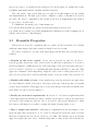
1.1
The Viewing Sphere
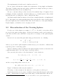
In this work, any scene observed from a fixed viewpoint at a given moment will be
modeled as the unit sphere centered at the viewpoint (S2 = {(x, y, z) ∈ R3 |x2 + y 2 + z 2 =
1}) on which each point has an associated color, the color that is seen when one looks
toward this point. Here we assume that the viewpoint is the origin of R3 for convenience.
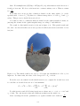
This sphere we will call the viewing sphere. Notice that the viewing sphere represents
the whole 360 degree longitude by 180 degree latitude field of view. Figure 1.1 shows an
example of viewing sphere.
6
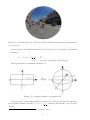
Figure 1.1: A viewing sphere (looked from outside) that represents the visible information
of some scene.
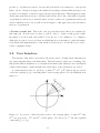
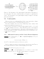
A very known and useful representation of S2 is the one by longitude and latitude
coordinates1 :
r : [−π, π] × − π2 , π2 → S2
(λ, φ) 7→ (cos(λ) cos(φ), sin(λ) cos(φ), sin(φ))
This representation is illustrated in figure 1.2.
Figure 1.2: Longitude/latitude representation r.
r gives us a way of representing all the information of a scene from a single viewpoint as
the longitude/latitude rectangle [−π, π] × − π2 , π2 , which we will call the equirectangular
domain.
1
Also known as yaw and pitch values or pan and tilt values.
7
Recent development of stitching techniques made it possible to take many pictures
of a scene and stitch them all together into an equirectangular domain that represents
such scene. More specifically, from a set of photographs (common photographs or images
obtained with fisheye lenses, for example) taken from the same viewpoint, it became
possible to create an image in which every pixel represents a point and its associated
color on the equirectangular domain.
The stitching process itself is a very detailed task and it is not going to be discussed
in this work. However, it is important to notice that without the development of such
techniques, it would not be possible to deal with projections from the viewing sphere to
an image plane, which is one of the main tasks of this thesis. For additional information
about stitching, we suggest references [2] and [3].
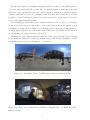
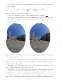
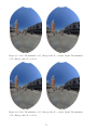
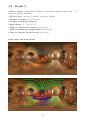
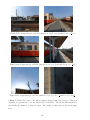
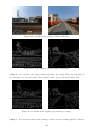
Such images of the equirectangular domain are called equirectangular images and will
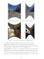
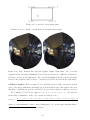
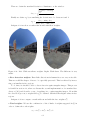
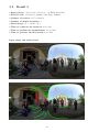
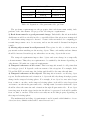
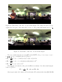
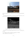
be the input information for all the algorithms that we will develop. Examples of equirectangular images are shown in figures 1.3, 1.4 and 1.5.
Figure 1.3: “San Marco Plaza”, by Flickr user Veneboer, taken from [10].
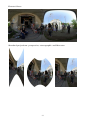
Figure 1.4: “Reboot 8.0: Ianus demos Cabinet to Thomas’ kid”, by Flickr user Aldo,
taken from [10].
8
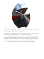
Figure 1.5: “Cloud Gate”, by Flickr user Wcm777, taken from [10].
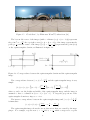
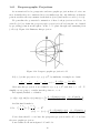
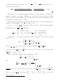
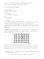
The bottom left corner of the images (with coordinates (x, y) = (m − 1, 0)) represents
the point −π, − π2 , the top right corner ((x, y) = (0, n − 1)) of the image represents the
point π, π2 and the center of the image ((x, y) = ( m−1
, n−1
)) represents the point (0, 0)
2
2
on the equirectangular domain, as illustrated in figure 1.6.
Figure 1.6: Correspondence between the equirectangular domain and the equirectangular
image.
The correspondence between [−π, π] × − π2 , π2 and the equirectangular image is very
simple:
φ + π2
λ+π
(λ, φ) 7→ (x, y) = (m − 1) −
(m − 1),
(n − 1) ,
π
2π
where m and n are the height and width of the equirectangular image and the image is
assumed to have coordinates in [0, m − 1] × [0, n − 1]. To keep the proportions of the
equirectangular domain we impose n = 2m.
The inverse correspondence between the equirectangular image and [−π, π] × − π2 , π2
is immediate:
2πy
π
πx
(x, y) 7→ (λ, φ) =
− π, −
.
n−1
2 m−1
The equirectangular image shows the strong distortions that are caused by the map-
ping r. For example, regions near φ = − π2 and φ =
9
π
,
2
which correspond to regions
near the south and north poles on the sphere, are too stretched. That happens because
the sphere has a much smaller area near the poles, for some variation of φ, than near the
equator (φ = 0) for this same variation of φ. But these very different areas are represented
by the same number of pixels on the equirectangular image.
To finish this discussion about equirectangular images, it is important to emphasize
how popular this format of image became during the last years. Today it is possible to
find thousands of them on photo sharing sites. To illustrate this point, the reader may,
for example, access Flickr group on [10].
One can find there a great variety of equirectangular images: indoor or outdoor scenes,
with or without people, realistic or with artistic effects, from places all around the world,
in many different resolutions.
1.2
Problem Statement
With the formalism created in the last section we can formulate the panoramic image
problem as the one of finding a mapping
u : S ⊆ S2 → R2
(λ, φ) 7→ (u, v)
,
with desirable properties. Here S is a field of view which may not be the entire 360 by
180 degree entire field of view.
The set u(S) can be interpreted as a continuous image: each u(λ, φ) ∈ u(S) receives
the color that the viewing sphere has at (λ, φ).
Thus we have two ways of thinking of a panoramic image: as a mapping u or as
a continuous image u(S). This duality allows us to turn perceptual properties of the
continuous image into algebraic expressions, that depend on the function u.
1.3
Standard Projections
There are many known functions that project the viewing sphere (or a part of it) onto
a plane. Many of them were developed for cartography purposes, since Earth’s shape
can be approximated by a sphere. There are different classifications for these projections
(equal-area, conformal, cylindrical, etc.). For details about these classifications and many
examples of projections, we recommend [11].
In this section we study the best known projections (Perspective, Stereographic and
Mercator) and discuss their properties.
1.3.1
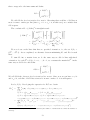
Perspective Projection
The result of a perspective projection is very well known because most of the photographs (taken with simple cameras) are captured by lenses that approximate linear
10
perspective, since this projection has many desirable properties that we are going to
discuss further.
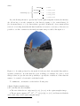
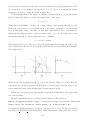
The construction of this projection is quite simple: the viewing sphere is projected
onto a tangent plane (we are going to use the plane x = 1) through lines emanating form
the center of the sphere, as shown in figure 1.7.
Figure 1.7: Perspective projection.
y z Q
y z
1, ,
'
,
∈ x=1 , which consists in a
x x
x x
simple division by the x coordinate. Observe that the mapping stretches to infinity when
Thus (x, y, z) ∈ S2 is mapped to
x → 0 and is not defined when x = 0. So we define the perspective only for points with
x > 0.
Since we want a mapping from the equirectangular domain to a plane, we have to
convert the formula above to latitude/longitude coordinates: given (x, y, z) ∈ S2 , x > 0,
there is a (λ, θ) ∈ − π2 , π2 × − π2 , π2 such that (x, y, z) = (cos(λ) cos(φ), sin(λ) cos(φ), sin(φ))
and the perspective projection is
sin(λ) cos(φ)
tan(φ)
sin(λ)
(cos(λ) cos(φ), sin(λ) cos(φ), sin(φ)) 7→ 1,
,
= 1, tan(λ),
.
cos(λ) cos(φ) cos(λ) cos(φ)
cos(λ)
Hence, the final formula for the perspective projection is:
π π π π
P : − ,
× − ,
→ R2
2 2
2 2
tan(φ)
(λ, φ) 7→ (u, v) = tan(λ),
cos(λ)
Figures 1.8 and 1.9 show some results of this projection with different fields of view.
11
Figure 1.8: Left: 90 degree long./90 degree lat.; Right: 120/120.
Figure 1.9: Left: 90 degree long./90 degree lat.; Right: 130/120.
The main advantages and disadvantages of the perspective projection are:
Advantages: • Straight lines in the scene appear straight on the final result;
• When the camera is held parallel to the ground the orientation constancy of the vertical
lines is maintained, i.e., they appear vertical in the resulting image.
Disadvantages: • As the field of view increases, the shape of the objects near the
periphery of the image starts to change considerably. This fact is noticeable even for
FOVs which are not too wide, such as 120 degrees (see the right images in figures 1.8 and
1.9). The cause of this effect is that the perspective projection is not conformal, concept
that we are going to formalize further. Informally, a mapping is conformal if it locally
12
preserves shapes of objects. The nonconformality of the perspective projection is the
reason why simple photographs have a small field of view, usually less than 90 degrees.
1.3.2
Stereographic Projection
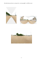
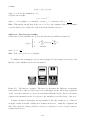
The geometric construction of the stereographic projection is the following: the viewing sphere is projected on the x = 1 plane (just as the perspective projection) through
lines emanating from the pole opposite to the point of tangency, (−1, 0, 0) in this case. So
it is essentially the perspective projection but with lines coming from (−1, 0, 0) instead
of coming from (0, 0, 0), as shown in figure 1.10.
Figure 1.10: Stereographic projection.
If (1, ŷ, ẑ) is the projection of (x, y, z) ∈ S2 , by similarity of triangles we obtain the
following relations:
ŷ
y
ẑ
z
=
, =
.
2
x+1 2
x+1
Q
2y
2z
2y
2z
2
Thus (x, y, z) ∈ S is mapped to 1,
,
'
,
∈ x=1 . Obx+1 x+1
x+1 x+1
serve that the mapping is not defined at (−1, 0, 0), the opposite pole to the tangent plane.
In longitude/latitude coordinates, we have:
2 sin(λ) cos(φ)
2 sin(λ)
(cos(λ) cos(φ), sin(λ) cos(φ), sin(φ)) 7→ 1,
.
,
cos(λ) cos(φ) + 1 cos(λ) cos(φ) + 1
So the final formula for the stereographic projection is:
h π πi
S : [−π, π) × − ,
\ {(−π, 0)} → R2
2 2
2 sin(λ) cos(φ)
2 sin(φ)
,
(λ, φ) 7→ (u, v) =
cos(λ) cos(φ) + 1 cos(λ) cos(φ) + 1
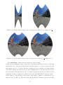
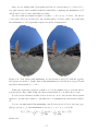
We show some results of this projection for different scenes in figure 1.11.
13
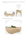
Figure 1.11: Left: 180 degree long./180 degree lat.; Right: 180/180.
The main advantages and disadvantages of the stereographic projection are:
Advantages: • Lines that pass through the center of the image are preserved;
• It is conformal, i.e., it preserves the shape of objects locally. Although the objects
near the periphery of wide fields of view are stretched, this stretching is the same in all
directions, which maintains the conformality of such mapping.
Disadvantages: • Most of the lines in the scene are bent on the final result.
1.3.3
Mercator Projection
This projection was presented by the flemish cartographer and geographer Gerardus
Mercator, in 1569, with only cartography purposes in mind.
It is a cylindrical projection, which means that the u coordinate varies linearly with the
longitude λ, and it is conformal. We are going to obtain its formula when we introduce the
Cauchy-Riemann equations on the next chapter, in order to formalize what is a conformal
mapping.
For the moment, it is just a cylindrical projection that preserve the shape of the
objects. Its formula is the following:
π π
M : [−π, π) × − ,
→ R2
2 2
(λ, φ) 7→ (u, v) = (λ, log(sec(φ) + tan(φ)))
Observe that the mapping tends to infinity when φ → ± π2 .
Figures 1.12 and 2.8 show some results of this projection.
14
Figure 1.12: 360 degree longitude/150 degree latitude.
Figure 1.13: 360 degree longitude/150 degree latitude.
The main advantages and disadvantages of the Mercator projection are:
Advantages: • As in all cylindrical projections, meridians ({(λ, φ) ∈ S2 : λ = constant})
are mapped to vertical lines.
• It is conformal.
• It handles wide longitude fields of view, even 360 degree ones.
Disadvantages: • Just as the stereographic projection, most of the straight lines in the
scene are bent on the final result.
1.4
Modified Standard Projections
In the last section, we showed the three most known projections from the viewing
sphere to an image plane. In this section, we show how simple modifications of these
projections can generate better results.
15
1.4.1
Perspereographic Projections
As we mentioned before, perspective and stereographic projections have a lot in common. Actually, they are constructed in a very similar way, the only difference is that the
point from where the rays emanate in the first is (0, 0, 0) and in the second is (−1, 0, 0).
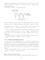
We generalize the geometrical construction of these both projections as follows: for
each K ∈ [0, 1] we define the perspereographic projection for K as being the one obtained
by projecting points from the sphere on the x = 1 plane through rays emanating from
(−K, 0, 0). Figure 1.14 illustrates this projection.
Figure 1.14: Perspereographic projection for K.
If (1, ŷ, ẑ) is the projection of (x, y, z) ∈ S2 , by similarity of triangles we obtain:
ŷ
y
ẑ
z
(1 + K)y
(1 + K)z
=
,
=
⇒ ŷ =
, ẑ =
.
1+K
x+K 1+K
x+K
x+K
x+K
Obviously this projection is not defined for (x, y, z) ∈ S2 such that x = −K. To
simplify, we are going to consider just the points s.t. x > 0.
In longitude/latitude coordinates:
(cos(λ) cos(φ), sin(λ) cos(φ), sin(φ)) 7→
(1 + K) sin(λ) cos(φ) (1 + K) sin(λ)
,
1,
cos(λ) cos(φ) + K cos(λ) cos(φ) + K
.
And the final formula is:
π π π π
P SK : − ,
× − ,
→ R2
2 2
2 2
(1 + K) sin(λ) cos(φ) (1 + K) sin(φ)
(λ, φ) 7→ (u, v) =
,
cos(λ) cos(φ) + K cos(λ) cos(φ) + K
Notice that when K = 0 we have the perspective projection and for K = 1 we have
the stereographic projection.
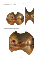
Some results are shown in figures 1.15 and 1.16.
16
Figure 1.15: Both with 150 degree long./150 degree lat. Left: K = 0; Right: K = 31 .
Figure 1.16: Both with 150 degree long./150 degree lat. Left: K = 23 ; Right: K = 1.
The advantages of these new projections are the following:
• They give us an intuitive way to control the conformality and the preservation of straight
lines in the scene. The greater the K the better the shapes of objects are preserved, and
the extreme case, K = 1, leads to the stereographic projection, which is conformal. On the
other hand, when lower values for K are used, straight lines become less bent and objects
more stretched. The extreme case, K = 0, leads to perspective projection. Therefore the
parameter K can be adjusted according to the scene and FOV that is being projected.
• The value K could depend on the points on the sphere. Thus we would have K as a
function of (λ, φ), K(λ, φ). This idea allows the possibility of having a projection locally
17
adapted to the image content. Possibly K(λ, φ) should have some degree of smoothness
and such analysis and results for this approach are going to be left as future work.
1.4.2
Perspective Projection Centered on Other Points
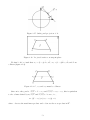
The perspective projection shown on section 1.3.1 preserves well only the shape of
objects that are near the point with (λ, φ) = (0, 0), the center of such projection.
As we’ll see in further sections, one may want to use perspective projection but preserve
shapes of other objects that are not near (λ, φ) = (0, 0). That leads to constructing
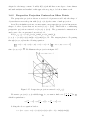
perspective projections centered on (λ0 , φ0 ) 6= (0, 0). The geometrical construction is
analogous to the one presented on section 1.3.1.
Let (x0 , y0 , z0 ) = (cos(λ0 ) cos(φ0 ), sin(λ0 ) cos(φ0 ), sin(λ0 )),
(x, y, z) = (cos(λ) cos(φ), sin(λ) cos(φ), sin(λ)) ∈ S2 . The tangent plane to S2 passing
through (x0 , y0 , z0 ) has the following equation:
Y
: x0 (x − x0 ) + y0 (y − y0 ) + z0 (z − z0 ) = 0
since (x0 , y0 , z0 ) ⊥
Q
Y
: x0 x + y0 y + z0 z = 1
. We illustrate the projection in figure 1.17.
Figure 1.17: Perspective projection centered on (λ0 , φ0 ).
We want to project (x, y, z) radially in
Q
, i.e., we want to find α s.t.
which is equivalent to
x0
x
α
− x0 + y 0
y
α
− y0 + z0
z
α
x y z Q
, ,
∈ ,
α α α
− z0 = 0.
Solving the above equation leads to
α = (x0 x + y0 y + z0 z) = (cos(φ0 ) cos(φ) cos(λ0 − λ) + sin(φ0 ) sin(φ)).
18
x y z So the projection (x, y, z) 7→
, ,
has the following form in (λ, φ) coordinates:
α α α
cos(λ) cos(φ)
(λ, φ) 7→
,
cos(φ0 ) cos(φ) cos(λ0 − λ) + sin(φ0 ) sin(φ)
sin(λ)
sin(λ) cos(φ)
,
.
cos(φ0 ) cos(φ) cos(λ0 − λ) + sin(φ0 ) sin(φ) cos(φ0 ) cos(φ) cos(λ0 − λ) + sin(φ0 ) sin(φ)
Observe that the projection is not well defined for (x, y, z) ∈ S2 s.t. x0 x+y0 y+z0 z = 0,
Q
the plane that is parallel to and passes through zero. This also happened for the simple
Q
perspective projection: the points s.t. x = 0 could not be projected in x=1 .
The final projection is in R3 and we would like it to have a 2D coordinate system.
Q
Q
This is achieved by performing two rotations on
in order to transform it in x=1 , for
example. We will not expose the details of this process here.
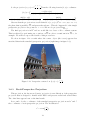
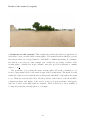
We show in figure 1.18 a result where the center object (the tower) appears less
stretched than in the standard perspective projection (right image in figure 1.8).
Figure 1.18: Perspective centered on (λ, φ) = (− π3 , π9 ).
1.4.3
Recti-Perspective Projection
This projection, also known as Pannini projection, is a modification of the perspective
projection that is designed to handle wider FOVs and preserve radial and vertical lines.
The other lines appear bent on the final result.
Let u and v be the coordinates of the standard perspective projection and u0 and v 0
the coordinates of recti-perspective projection. The modification
λ
0
u = α tan
,
α
19
where alpha is a chosen parameter, allows this projection to handle wider FOVs and
preserves vertical lines (λ constant ⇒ u0 constant).
In order to preserve radial lines, the v coordinate of the perspective projection must
be scaled by a constant multiple of the factor used to scale the u axis, i.e.,
0
u
0
v = γv, γ = β
,
u
where β is a chosen parameter. The above expressions lead to
λ
tan(φ)
βα
tan
α
, if λ 6= 0,
v0 =
sin(λ)
and
v 0 = β tan(φ), if λ = 0.
We show in figure 1.19 a good result obtained setting α = 2 and β = 34 :
Figure 1.19: 180 degree longitude/130 degree latitude.
1.5
Previous Approaches
As pointed in last sections, it is not an easy task to obtain an image from a wide field
of view. We showed some of the most known projections from the sphere to an image
plane and realized that all of them have their advantages and disadvantages.
This section is devoted to discuss previous approaches created during the last years
to deal with the problem of distortions in panoramic images. We do not intend to get
into too many details of each approach, but we intend to show their key ideas in order to
motivate the next chapter. Thus, this section is intended to be a review and a motivation.
20
We chose to discuss three papers that we understand to have the key ideas on the
development of this theme: [5], [6] and [7]. At the end of the section, we mention some
other important related work.
1.5.1
Correction of Geometric Perceptual Distortions in Pictures
This work by Zorin and Barr ([5]) is surely one of the most referenced in this area. It
is probably the first work to apply perceptual principles to the analysis and construction
of planar images of the 3D world. Their theory is even more applicable for panoramic
images, where deviations of perception are more present.
The authors mention that the most important features that an image should have to
be representative are the structural features such as dimension (whether the image of an
object is an area, a curve or a point) and presence or absence of holes and self-intersections.
They make the following statement:
The retinal projections of an image of an object should not contain any structural
features that are not present in any retinal projection of the object itself.
Since most of the visual informations that we have are in the images formed on the retina,
this statement asks that when we look at an image the objects should not contain any
structural feature that we would not see if we looked directly at them.
They selected three structural requirements to develop their theory:
• The image of a surface should not be a point;
• The image of a part of a straight line either should not have self intersections (loops)
or else should be a point;
• The image of a plane should not have twists on it, i.e., either each point of the plane is
projected to a different point in the image, or the whole plane is projected to a curve.
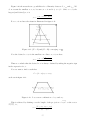
Figure 1.20 illustrates the last two requirements:
Figure 1.20: Mappings forbidden by the last two requirements.
They also state desirable conditions. These are not as essential as the structural ones
because they can be changed with some intervals of tolerance. The desirable conditions
are the following:
• Zero-curvature condition: Images of all possible straight lines should be straight;
21
• Direct view condition: All possible objects in the image should look as if they were
viewed directly - as if they appeared in the middle of a photograph.
The authors obtain two functionals, K and D, that measure how much a mapping
Tsphere from the viewing sphere to a plane does not respect both conditions. So ideally
we should find a map such that:
K(Tsphere ) = D(Tsphere ) = 0;
After a theoretical development, it is shown that there is no Tsphere satisfying these
conditions and also the structural requirements. Then they suggest to minimize the
functional
F (Tsphere ) = µK(Tsphere ) + (1 − µ)D(Tsphere ),
where µ is the desired tradeoff between both desirable conditions.
An approximate minimizer for this functional is a perspective projection of the viewing
sphere followed by a one-to-one smooth transformation of the image plane given by:
√
r
R( r2 + 1 − 1)
ρ = λ + (1 − λ) √
; ψ = φ,
R
r( R2 + 1 − 1)
where (r, φ) is the polar coordinate system of the perspective image, (ρ, ψ) is the polar
coordinate system of the transformed image, λ is a parameter that depends on µ and R
depends on the FOV that is being projected.
Some results for different values of λ are shown in figures 1.21 and 1.22.
Figure 1.21: Both: 150 degree longitude/150 degree latitude. Left: λ = 0 (very similar
to stereographic projection); Right: λ = 1 (perspective projection).
22
Figure 1.22: Both: 150 degree longitude/150 degree latitude. Left: λ = 12 ; Right: Perspereographic projection for K =
1
.
2
Both have the same purpose of controlling the
conformality and straight lines in the scene. Which one is better? The choices λ =
K=
1
2
1
2
and
are arbitrary.
The key ideas that we can take from this work are: a panoramic image should respect
the structural requirements; no panoramic image (mapping from the viewing sphere to
a plane) that satisfies the structural requirements can satisfy completely both desirable
properties at the same time; an optimization framework is an option for the task of
minimizing all the important distortions.
1.5.2
Artistic Multiprojection Rendering
As we have already mentioned, perspective projection causes too much distortion for
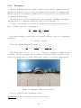
wide-angle fields of view. A simple and effective alternative to such problem is to render
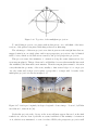
the most distorted objects in a different way.
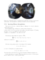
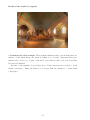
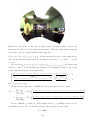
This alternative was already known and used by painters hundreds of years ago, for
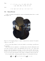
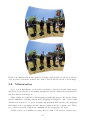
example, in Raphael’s School of Athens (Figure 1.23). The humans in the foreground
would appear too distorted if rendered with the same perspective projection of the background. So Raphael altered the projections of the humans to give each one a more central
perspective projection. This choice did not take off (actually improved) the realism of the
painting.
This work by Agrawala, Zorin and Munzner ([6]) suggests using the same method for
computer-generated images and animations: a scene is rendered using a set of different
cameras. One of this cameras is elected to be the master camera, which is going to be
used to render the background, and the other ones are the local cameras, which are going
to be used to render the objects in the scene.
The visibility is not a well defined problem in this context. They use the visibility
23
Figure 1.23: Raphael’s School of Athens.
ordering of the master camera to solve this problem: a point will be rendered if it is visible
for the master camera.
The key idea that we have to take from this paper is that a special treatment can
be given to the objects in order to reduce their distortion in panoramic images. But the
multiprojection rendering has also other applications:
• Artistic Expression: The usage of different viewpoints was used by painters also to
express feelings, ideas and mood.
• Best Views: A good viewpoint for an object may not be the best viewpoint for other
objects. By choosing the best viewpoint for each object in the scene it’s possible to
improve the representation of the scene.
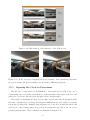
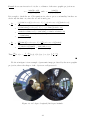
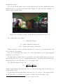
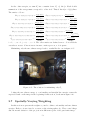
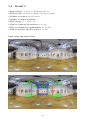
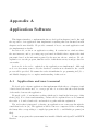
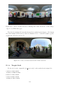
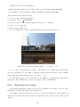
The author of this thesis, in a final course project, adapted the techniques described
in this article for real world scenes in the following way: a set of equirectangular images
(views) is given to the user so he can choose a different perspective (camera) for each
view, by setting the FOV and the center point of each perspective. A screenshot of the
first window of the user interface is shown in figure 1.24.
In the next windows, the user specifies which of the perspectives is the best view for
each object and the program tries to solve the visibility problem for the master camera.
An output of the program is the right image in figure 1.25, where I rendered myself with
a local camera (perspective projection centered on me), to correct my distortions on the
left image.
The reader may check the home page with more results and details of this project:
[12].
24
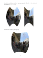
Figure 1.24: First window of the interface of the S3D project.
Figure 1.25: Both: 90 degree longitude/90 degree latitude. Left: Standard perspective
projection; Right: Me (black t-shirt) corrected with a different perspective.
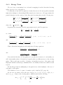
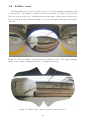
1.5.3
Squaring the Circle in Panoramas
The key idea of this article by Zelnik-Manor, Peters and Perona ([7]) is the one of
constructing a projection that depends more on the structure of the entire scene, not only
where the objects are, like the previous approach we just presented.
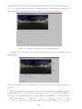
They start by discussing global projections (the ones we have already discussed under
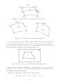
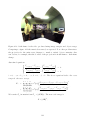
the name of standard projections), and suggest a multi-plane projection that is constructed in the following way: multiple tangent planes are positioned around the sphere and
each region of the viewing sphere is projected via perspective projection onto its corresponding tangent plane. This construction is illustrated in figure 1.26.
25
Figure 1.26: Top view of the multiplane projection.
To unfold this projection on a plane without distortions, one could think of the intersections of the planes being fitted with hinges that allow flattening.
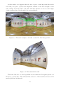
The advantages of this new projection are that it preserves the straight lines that are
mapped entirely in one single plane and it uses perspective projections only for limited
fields of view, which avoids distortions caused by the global perspective projection.
This process causes discontinuities of orientation along the seams (intersections between tangent planes). This problem can be well hidden for scenes that naturally have such
discontinuities, like man-made environments. Then the tangent planes must be chosen in
a way that fits the geometry of the scene, usually so that vertical edges of a room project
onto the seams and each projection plane corresponds to a single wall. A result of the
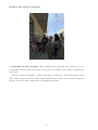
multi-plane projection is shown in figure 1.27.
Figure 1.27: 180 degree longitude/90 degree longitude. Source image: “Posters”, by Flickr
user Simon S., taken from [10].
Under this projection the objects on the scene still may appear distorted on the final
result for two reasons: if an object falls on a seam, it will have a discontinuity of orientation
on it, which is very unnatural; or even for reduced FOVs, the perspective projection still
26
can distort objects..
The solution adopted for these two kinds of distortion is very similar to the one used
on [6]: the background is rendered using the multi-plane projection and the objects are
rendered each one using a local perspective projection centered on it.
The author of this thesis implemented most of the techniques contained in this article
in his Image Processing course final project. The reader can see the details in [13].
1.5.4
Other Approaches
In this section we expose very briefly three other approaches ([14], [4] and [8]) that
also deal with the problem of constructing panoramic images:
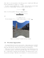
1) Photographing Long Scenes with Multi-Viewpoint Panoramas ([14]): This
work addresses the problem of making a single image of a long planar scene (the buildings
of one side of a street, for example) having as input a set of photographs taken from
different viewpoints. Although this problem is different from the one we are concerned
about in this thesis (here the input comes from a single viewpoint), it faces similar difficulties, such as preserving shapes of objects and making the final result a comprehensive
representation for the scene.
2) Capturing and Viewing Gigapixel Images ([4]): This article presents a viewer
that interpolates between cylindrical and perspective projection as the FOV is increased
or decreased. The ability for zooming in and out panoramas is more useful when the input
has high resolution. We think that the perspereographic projection presented in section
1.4.1 is a simpler solution for this task and could also produce good results.
3) Locally Adapted Projections to Reduce Panorama Distortions ([8]): This
work starts with a cylindrical projection of a scene and allows the user to mark regions
where he or she wants the projection to be near-planar. Then the method computes
a deformation of the projection cylinder that fits such constraints and smoothly varies
between different regions and unfold the deformed cylinder on a plane. Although their
results are very good in many cases and produced quickly via optimization, their method
has limitations: if some marked region occupies a wide-angle FOV (up to 120 degrees) the
final result starts suffering with the same limitations as perspective projection (stretching
of objects); a good solution depends on the precision of the user in marking regions; even
inside the marked regions lines may appear slightly bent; and if two marked regions are
too close, orientation discontinuities may appear between these regions, similarly to the
method presented in section 1.5.3.
27
Chapter 2
Optimizing Content-Preserving
Projections for Wide-Angle Images
In this chapter we show and discuss in more depth the ideas presented in Carroll et
al. ([1]), which we believe to be the state-of-the-art reference for the panoramic image
problem. Many details that are going to be exposed here do not appear in the original
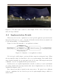
reference, which makes this chapter a good complement for it. We show in figure 2.1 a
result produced by this method.
Figure 2.1: A result produced by the method described in this chapter. FOV: 285 degree
longitude/170 degree latitude. Observe how most of the lines in the scene are straight
and the shape of the objects is well preserved.
Motivated by chapter 1, we start this chapter by making a list of desirable properties
in panoramic images and how this approach satisfies most of them.
Then we detail each section of the article in a mathematical way: all the necessary
definitions and theorems are going to be stated. The pre-requisites for understanding the
28
theory are going to be mentioned progressively. For the moment, we assume the reader
is familiar with multi-variable calculus and linear algebra.
The only parts of the article that are not explored in this chapter are the results
and implementation. The first topic is left to Chapter 3, where a discussion about it is
provided. We leave to Appendix A the details about how we implemented the method
we are going to describe here.
To summarize, the main goals of this chapter are:
• To list the main desirable properties in wide-angle images (section 2.1);
• To make an as complete as possible mathematical explanation for the techniques in [1]
(all the other sections of this chapter).
2.1
Desirable Properties
This section is devoted to argument why we consider [1] the best method for dealing
with panoramic images and why a study in depth about it is worthy.
We believe a method to produce wide-angle images should have the following characteristics:
• Depend on the scene content: As we saw in sections 1.3 and 1.4, global projections produce distortions. One of the reasons for this fact is that they do not give a
special treatment for different regions of the panorama. Some previous approaches (sections 1.5.2 and 1.5.3) tried to do something like this, but they did it in a coarse way. This
approach constructs a wide-angle image adapted to the location of lines (sections 2.2, 2.5
and 2.7), faces (sections 2.7 and B.1) and importance of regions on the scene (section 2.7).
• Handle wide fields of view: Some standard projections and previous approaches
are only defined for fields of view up to 180 degree and some of them produce bad results
even for narrower FOVs. This approach does not have this problem and can handle arbitrary FOVs, as can be seen in chapter 3.
• Satisfy the structural requirements: In section 1.5.1 we stated requirements that
a wide-angle image should have in order to match our perception of the world, since they
are based on the retinal projections. We do not devote any special discussion to them
here but we will always be careful to weather the method satisfy them or not.
• Have a simple user interface: Although not emphasized in the last chapter, some
previous approaches (sections 1.5.2, 1.5.3 and 1.5.4(3)) needed a precise and/or tedious
interaction with the user in order to yield a good result. The interface proposed in this
approach requires the user only to click the endpoints of a lines in the real world and set
29
their orientation. Details are presented in sections 2.2 and A.1.
• Mathematically formalize distortions and use an optimization framework:
Many previous approaches used just intuitive and classical ideas for minimizing distortions as, for example, centering projections on objects. A more precise solution would be
to mathematically formalize these distortions and try to minimize them all, in the way
we saw in section 1.5.1. All this chapter is devoted to develop such optimization solution.
• Preserve straight lines: It is very unnatural and noticeable if a line that is supposed to be straight in the final result appears bent. That happens because we perceive
all straight lines in the real world as straight. This approach handles this task by allowing the user to mark curves on the equirectangular image that should map to straight
lines on the final result (section 2.2), by obtaining an energy that measures how much
a marked curve is not straight in the final result (section 2.5) and then minimizing this
energy among with other energies (section 2.8).
• Have orientation consistency: Another undesirable effect related to lines is when a
line that is supposed to have some orientation (like the corner between walls or a tower
are supposed to be vertical) appear with another orientation in the result. This approach
avoids this problem by allowing the user to specify the orientation of lines (section 2.2)
and by obtaining an energy that measures how much a line deviates from the assigned
direction (section 2.5.1).
• Preserve shape of objects: Object distortion is another very unpleasant effect that
may appear in wide-angle images. Previous approaches (sections 1.5.2 and 1.5.3) tried
to fix this problem by locally correcting the projection of objects. This approach formalizes the concept of preservation of object shapes through the mathematical concept of
conformality. Section 2.4 is devoted to explain such concept and obtain an energy that
measures how conformal a panoramic image is. This energy is minimized together with
other energies in section 2.8.
• Vary scale and orientation smoothly: Discontinuities of scale and orientation may
be unpleasant. For example, when the approach in section 1.5.3 is applied to scenes that
do not have some natural discontinuity the result is not good (the unnatural discontinuities can be noticed on the ceiling of the scene in figure 1.27, for example). In section 2.6
we describe an energy that measures how smooth a panoramic image is. This energy is
also minimized among other ones.
• Avoid restrictions to some particular structure of scene: The method should
30
produce good results in a variety of scenes and it should not be restricted to some special
kinds of scene. All previous approaches suffered from this problem in different degrees. As
we will see in chapter 3, this new approach succeeds in this task. That happens because
all the important distortions are considered and well modeled. Also, this method depends
on parameters, and it is not desirable when one has to find a set of parameters that work
well for different scenes. As we will see in in chapter 3, this approach works well with a
fixed set of parameters.
• Produce results fast: This is the only property listed here that is not satisfied by
this approach. It is the price we have to pay in order to obtain a really precise result.
In chapter 3 we show that each result took about one or two minutes to be computed.
Although one can see it as a problem, we think that it is an incentive to study the numerical details and implementation of the method and develop tools and theory in order to
reduce computation time.
2.2
User Interface
The interface that will be shown here allows the user to identify linear structures in
the equirectangular image and mark them. Then the method will focus on making only
this specified linear structures to be straight in the final result, which is a more intelligent
solution than trying to make straight all possible lines, as the perspective projection.
(w)
(w)
A central question here is: given two points P1 , P2
∈ R3 what is the projection
of the line segment (r(w) ) connecting them on the viewing sphere? See the illustration in
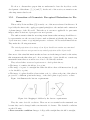
figure 2.2.
(w)
Figure 2.2: Projection of lines from the scene to the viewing sphere. Points P1
(w)
P2
(s)
are projected to P1
(s)
(s)
connecting P1 to P2 .
and
(s)
P2
and
on the sphere. We denote by r(s) the line segment
31
The key observation is that r(w) and r(s) project to the same points on the viewing
(s)
sphere (the arc connecting P1
points
(s)
P1
and
(s)
P2
(s)
and P2
on the sphere). So we can work just with the
2
∈ S , which will be corresponding points to the ones marked by the
user on the equirectangular image.
A very simple parametrization for r(s) is:
r(s) : [0, 1] → R3
(s)
(s)
t 7→ (1 − t)P1 + tP2
.
The projection of r(s) on S2 (say γ (s) ) also has a simple parametrization:
γ (s) : [0, 1] → S2
(s)
(s)
.
(1 − t)P1 + tP2
t 7→
(s)
(s)
k (1 − t)P1 + tP2 k
We have to bring these calculations to the equirectangular domain: The user marks
two points
h π πi
(λ1 , φ1 ) and (λ2 , φ2 ) ∈ [−π, π] × − ,
,
2 2
which have the following corresponding points on S2 :
(s)
P1 = (cos(λ1 ) cos(φ1 ), sin(λ1 ) cos(φ1 ), sin(φ1 )) and
(s)
P2 = (cos(λ2 ) cos(φ2 ), sin(λ2 ) cos(φ2 ), sin(φ2 )).
Let γ (s) as above. For each γ (s) (t) = (x(t),
z(t)) ∈ S2 , t ∈ [0, 1], we have to find
h π y(t),
πi
the corresponding (λ(t), φ(t)) ∈ [−π, π] × − , .
2 2
Let t0 ∈ [0, 1] and γ (s) (t0 ) = (x, y, z) and (λ, φ) the corresponding longitude and
latitude on the equirectangular domain. Then we have the following relation
(x, y, z) = (cos(λ) cos(φ), sin(λ) cos(φ), sin(φ)).
Obviously
φ = arcsin(z).
To obtain λ we first consider x > 0: in this case we must have − π2 < λ <
π
2
and the
relation
y
sin(λ) cos(φ)
=
= tan(λ)
x
cos(λ) cos(φ)
implies λ = arctan
y
x
.
Now consider x < 0, y < 0: for such points on the sphere we must have −π < λ < − π2
and λ = arctan xy − π satisfies such inequality and the relations between x, y and λ.
Analogously, for x < 0 and y > 0 the solution is λ = arctan xy + π.
For points s.t. x = 0, y < 0 the correspondent longitude is λ = − π2 and for x = 0,
y > 0 we have λ = π2 . To summarize:
λ = arctan 2(y, x),
32
where

y

arctan



x

y

arctan
−π

x

arctan 2(y, x) =
arctan xy + π




− π2




π
2
, x>0
, x < 0, y < 0
, x < 0, y > 0
, x = 0, y > 0
, x = 0, y < 0
Beyond allowing the user to specify lines1 in the equirectangular domain, the interface
also allows her to set the orientation of the lines by typing ‘v’ (for vertical lines), ‘h’
(for horizontal lines) or ‘g’ (for lines with no specified orientation). As we mentioned in
section 2.1, it is important that the final result has orientation consistency. If it were not
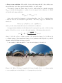
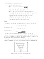
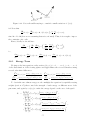
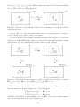
possible to set line orientations, the final panoramic image would be like figure 2.3.
Figure 2.3: A result produced by the method if the user had only marked lines with no
specified orientation. It seems that the tower is falling, for example. In order to avoid
such problem, we give the user the possibility to specify the orientation of lines that she
wants to be vertical or horizontal on the final result.
To summarize, our interface works in the following way:
• Input: Equirectangular image;
• For each line the user identifies
• The user clicks the two endpoints (λ1 , φ1 ), (λ2 , φ2 ) on the equirectangular image;
(s)
(s)
• The program computes P1 , P2 , γ (s) , (γ(t), φ(t)), t ∈ [0, 1], and draws in black the
curve (λ(t), φ(t)) on the equirectangular image;
1
Here line stands for both r(s) and γ (s) .
33
• The user types ‘v’, ‘h’ or ‘g’ for the orientation and the color of the curve changes.
• Output: Marked equirectangular image and a list of points2 .
We show in figure 2.4 an image produced by the process just explained:
Figure 2.4: Equirectangular image with lines marked by the user. Red lines stands for
vertical lines, blue for horizontal ones and green for general orientation ones.
For such marked lines, the method produces the result shown in figure 2.5.
Figure 2.5: Observe that line orientation is correct now. For example, the tower appears
vertical on the result, because the user specified such behavior.
2
The details of this list are left to section A.2.
34
The implementation details can be found in section A.2.
In our opinion, this interface satisfies the requirement of being simple and intuitive.
The tasks of clicking endpoints and setting orientations are simple and the procedure to
mark all the lines takes about one minute long.
We try to automate this procedure in section B.2 with the help of Computer Vision
techniques. It turns out that the obtained results are a good initial guess for lines, which
may help the user, avoiding her to have to mark all the lines.
One final remark is that the interface showed here is simpler than the one implemented
in [1]. Our input is an equirectangular image that represents the entire viewing sphere.
In [1] the input may have arbitrary FOVs and other formats, not only equirectangular.
Despite simpler, our interface serves our purposes well.
2.3
Discretization of the Viewing Sphere
For the rest of this chapter we assume S = S2 , i.e., the field of view that will be
projected is the entire viewing sphere. All the development is analogous if restricted to
some narrower FOV, since such FOV corresponds to a rectangle on the equirectangular
domain.
In section 1.2 we stated the panoramic image problem as the one of finding
u:
S2 → R2
(λ, φ) 7→ (u(λ, φ), v(λ, φ))
,
where (λ, φ) are in the equirectangular domain and (u, v) are cartesian coordinates that
represent position on the image plane.
Instead of finding a function defined in all equirectangular domain, we discretize it in
a uniform manner and look for the values of u at the vertices.
More precisely, the vertices of the discretization3 of the domain are
Λij = (λij , φij ), j = 0, . . . , n, i = 0, . . . , m,
where
2π
π
π
, φij = − + i , j = 0, . . . , n, i = 0, . . . m,
n
2
m
and the corresponding values of u at Λij are
λij = −π + j
uij = u(λij , φij ) = (uij , vij ), j = 0, . . . , n, i = 0, . . . m.
Figure 2.6 illustrates what was just explained.
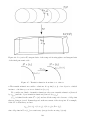
The image of each rectangle by the function r on the sphere is called quad.
In the next sections, we are going to formulate energy terms that depend on the values
uij and vij and measure how much a panoramic image contains undesirable distortions.
3
This discretization does not have to be the pixel discretization of the equirectangular image.
35
Figure 2.6: The discretization of the equirectangular domain induces a discretization of
the viewing sphere. The vertices of this discretization of the sphere (or, equivalently, the
vertices of the discretization of the equirectangular domain) are mapped to the image
plane by the function u.
2.4
Conformality
This section is devoted to mathematically model the concept of preservation of shapes
stated as a desirable property for wide-angle images in section 2.1.
The reader is assumed to have some notions of differential geometry of surfaces. Such
notions can be found in [15], sections 2.1 to 2.5.
Here a point (λ, φ) is an interior point in the equirectangular domain, i.e., λ 6= ±π and
φ 6= ± π2 . This assumption allows us to consider differential properties of the mapping u
and turns r into an actual parametrization. Although now this parametrization does not
cover the entire sphere (it excludes one meridian and the poles), we identify r((−π, π) ×
(− π2 , π2 )) as S2 , for convenience.
2.4.1
Differential Geometry and the Cauchy-Riemann Equations
Definition 2.1 A dipheomorfism ϕ : S → S is a conformal mapping if for all p ∈ S
and for all v1 , v2 ∈ Tp S holds
hdϕp (v1 ), dϕp (v2 )i = Θ2 (p)hv1 , v2 i,
where Θ2 is a differentiable function on S that never vanishes.
The above definition says that dϕp preserves inner products (except for the Θ2 factor).
The following statement proves that conformal mappings preserve angles:
Statement 2.1 Conformal mappings preserve angles.
Proof: Let ϕ : S → S be a conformal mapping. Let α : I → S and β : I → S two curves
in S that intersect in, say, t = 0. The angle θ between them at t = 0 is given by
cos(θ) =
hα0 (0), β 0 (0)i
, 0 < θ < π.
k α0 (0) kk β 0 (0) k
36
ϕ transform such curves in curves ϕ ◦ α : I → S, ϕ ◦ β : I → S that intersect at t = 0,
forming an angle given by:
cos(θ) =
hdϕα(0) (α0 (0)), dϕβ(0) (β 0 (0))i
Θ2 hα0 (0), β 0 (0)i
=
= cos(θ).
k dϕα(0) (α0 (0)) kk dϕβ(0) (β 0 (0)) k
Θ2 k α0 (0) kk β 0 (0) k
The definition of conformal mappings turns up to be appropriate for modeling preservation of shapes: according to definition 2.1, locally, the objects can only be rotated
and/or scaled in an equal manner along all directions. As we saw in statement 2.1, this
also implies in the preservation of angles.
We bring the formal discussion into the panoramic image context by taking in the
2
2
definition of conformality
πS π=S , S = R and ϕ = u.
Let p ∈ (−π, π) × − ,
. The basis of Tp S2 associated to r (the longitude/latitude
2
2
∂r
∂r
(p),
(p) , where
parametrization) is
∂λ
∂φ




− sin(λ) cos(φ)
− cos(λ) sin(φ)




∂r
∂r
(p) = 
(p) 
and
cos(λ) cos(φ) 
− sin(λ) sin(φ) 



.
∂λ
∂φ
0
cos(φ)
Assuming u to be a dipheomorfism dup : Tp S2 → Tu(p) R2 = R2 has the following
form4 :
∂u
(p)
 ∂λ
dup (w) =  ∂v
(p)
∂λ

∂u
(p)

∂φ
∂r
∂r
 w{ ∂λ
(p), ∂φ
(p)} ,
∂v
(p)
∂φ
∂r
∂r
where w{ ∂r (p), ∂r (p)} is a vector in Tp S2 written in the basis
(p),
(p) .
∂λ
∂φ
∂λ
∂φ
∂r
∂r
It’s clear that
(p) and
(p) are orthogonal, but they are not unitary, since
∂λ
∂φ
∂r (p) = | cos(φ)| = cos(φ).
∂λ Thus we define the following orthonormal basis for Tp S2 :
!
\
0
∂r
∂r
(p) =
(p) =
∂φ
∂φ
1
∂r
∂r
(p), ∂φ
(p)}
{ ∂λ

and


1
\
∂r
1 ∂r
(p) =
(p) =  cos(φ) 
∂λ
cos(φ) ∂λ
0
.
∂r
∂r
(p), ∂φ
(p)}
{ ∂λ
!
!
\
\
∂r
∂r
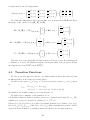
Lemma 2.1 u : S2 → R2 is conformal if and only if dup
(p) = R±90 ·dup
(p) ,
∂φ
∂λ
!
!
π π
0 −1
0 1
∀p ∈ (−π, π) × − ,
, where R90 =
, R−90 =
= −R90 are 90
2 2
1 0
−1 0
degree rotations.
4
Details in [15], pages 84 and 85.
37
π π
Proof: (⇐) We want to prove that u is conformal. Let p ∈ (−π, π) × − ,
and
2 2
\
\
\
\
∂r
∂r
∂r
∂r
v1 , v2 ∈ Tp S2 . Suppose v1 = α1 (p) + β1 (p) and v2 = α2 (p) + β2 (p). It’s clear
∂φ
∂λ
∂φ
∂λ
that
hv1 , v2 i = α1 α2 + β1 β2 ,
\
\
∂r
∂r
(p) and
(p) are orthonormal. Now consider
∂φ
∂λ
∂[
r
∂[
r
∂[
r
∂[
r
hdup (v1 ), dup (v2 )i = hα1 dup ∂φ
(p) + β1 dup ∂λ
(p) , α2 dup ∂φ
(p) + β2 dup ∂λ
(p) i
2
∂[
r
∂[
r
∂[
r
.
= α1 α2 dup ∂φ
(p) + α1 β2 hdup ∂φ
(p) , dup ∂λ
(p) i+
2
∂[
r
∂[
r
∂[
r
(p) , dup ∂φ
(p) i + β1 β2 dup ∂λ
(p) +β1 α2 hdup ∂λ
since
Applying the hypothesis, we have
∂[
r
∂[
r
∂[
r
∂[
r
hdup ∂φ (p) , dup ∂λ (p) i = hdup ∂λ (p) , dup ∂φ (p) i = 0
and
∂[
r
∂[
r
(p) = dup ∂λ
(p) dup ∂φ
and we obtain
2
2
∂[
r
∂[
r
(p) (α1 α2 + β1 β2 ) = dup ∂φ
(p) hv1 , v2 i.
hdup (v1 ), dup (v2 )i = dup ∂φ
∂[
r
Taking Θ(p) = dup ∂φ (p) in the definition of conformality, we conclude that u is
conformal.
(⇒) Now suppose that u is conformal, i.e.,
hdup (v1 ), dup (v2 )i = Θ(p)2 hv1 , v2 i, ∀v1 , v2 ∈ Tp S2 .
∂[
r
∂[
r
∂[
r
∂[
r
(p) and v2 = ∂λ
(p) leads to hdup ∂φ
(p) , dup ∂λ
(p) i = 0, i.e.,
• Taking v1 = ∂φ
∂[
r
∂[
r
(p) and dup ∂λ
(p) are orthogonal.
dup ∂φ
∂[
r
∂[
r
∂[
r
• Taking v1 = v2 = ∂φ
(p) we obtain dup ∂φ
(p) = |Θ(p)|. Taking v1 = v2 = ∂λ
(p)
∂[
r
∂[
r
∂[
r
leads to dup ∂λ
(p) = |Θ(p)|. Thus dup ∂φ
(p) = dup ∂λ
(p) .
The two above considerations, dup
∂[
r
(p)
∂φ
and dup
∂[
r
(p)
∂λ
the same length in R2 , allows only two possibilities: dup
∂[
r
∂[
r
dup ∂φ
(p) = R−90 · dup ∂λ
(p) .
are orthogonal and have
∂[
r
∂[
r
(p)
=
R
·
du
(p)
or
90
p ∂λ
∂φ
38
We call
!
h = dup
\
∂r
(p)
∂φ
∂u
(p)
 ∂λ
=  ∂v
(p)
∂λ

the differential north vector and

∂u
!
(p)
\
∂r

k = dup
(p) =  ∂λ
∂v
∂λ
(p)
∂λ

∂u
(p)

∂φ

∂v
(p)
∂φ
0
!
1

∂u
(p)


=  ∂φ

∂v
(p)
∂φ




∂u
1
(p)
1 
  cos(φ) 
∂φ
=


∂v
cos(φ)
(p)
0
∂φ

∂u
(p) 
∂λ

∂v
(p)
∂λ
the differential east vector.
The lemma tells us that u conformal is equivalent to h = R90 k or h = R−90 k. Both
possibilities are shown in figure 2.7.
Figure 2.7: We exclude the second possibility above.
We ask u to preserve the orientation of the orthonormal basis of the tangent plane,
i.e., we forbid h = R−90 k.
This choice avoids a mirroring effect that could appear on the final result.
With these new considerations we restate the lemma:
Theorem 2.1 (Cauchy-Riemann Equations) Let p = (λ, φ) ∈ (−π, π) × − π2 , π2 . u :
S2 → R2 is a conformal mapping that preserves the orientation of the orthonormal basis
of Tp S2 if and only if
∂u
1 ∂v
∂v
1 ∂u
(p) = −
(p) and
(p) =
(p).
∂φ
cos(φ) ∂λ
∂φ
cos(φ) ∂λ
Proof: u conformal mapping that preserves orientation ⇔ h = R90 k ⇔
=
0 −1
1
0
!
1
cos(φ)
1
cos(φ)
∂u
(p)
∂λ
∂v
(p)
∂λ
!
(
⇔
∂u
(p)
∂φ
∂v
(p)
∂φ
1
∂v
= − cos(φ)
(p)
∂λ
=
1 ∂u
(p)
cos(φ) ∂λ
∂u
(p)
∂φ
∂v
(p)
∂φ
!
=
.
Despite of being a little abuse of nomenclature, from now on we consider the fact of
u : S2 → R2 being conformal equivalent to u satisfying the Cauchy-Riemann Equations.
The C-R equations are an analytical and practical way of checking conformality.
39
2.4.2
Examples
This section illustrates the theory that we just developed with two mappings u already
discussed in chapter 1: there we just used intuition and perception to argument that
Mercator (section 1.3.3) and Stereographic (section 1.3.2) projections are conformal. Here
we argument it analytically.
The Mercator projection is a cylindrical projection designed to maintain conformality.
The imposition u = λ makes it cylindrical because u is proportional to λ.
To impose conformality, we use the C-R equations and determine the expression for
the v coordinate: from the second equation
∂v
1
∂u
1
=
·
.
=
∂φ
cos(φ) |{z}
∂λ
cos(φ)
1
From basic calculus, we know that one possible solution for the above differential
equations is
v = log(sec(φ) + tan(φ)).
Such v also satisfies the first C-R equation:
∂u
1
1 ∂v
=0=−
·0=−
∂φ
cos(φ)
cos(φ) ∂λ
Thus the projection (λ, φ) → (u = λ, v = log(sec(φ) + tan(φ))) is cylindrical and
conformal. We show in fugure 2.8 an example of wide-angle image generated by the
Mecator projection, where we can see that, in fact, shapes of objects are well-preserved:
Figure 2.8: Example of Mercator projection.
Now we consider the stereographic projection:
Statement 2.2 The stereographic projection is conformal.
40
Proof: As we saw in section 1.3.2, the coordinates of the stereographic projection are
u=
2 sin(φ)
2 sin(λ) cos(φ)
and v =
.
cos(λ) cos(φ) + 1
cos(λ) cos(φ) + 1
It’s enough to check the two C-R equations in order to prove conformality, but here we
check only the first one, since the second is analogous:
∂
∂
[ ∂φ
(2 sin λ cos φ)][cos λ cos φ + 1] − [ ∂φ
(cos λ cos φ + 1)][2 sin λ cos φ]
∂u
•
=
∂φ
(cos λ cos φ + 1)2
[−2 sin λ sin φ][cos λ cos φ + 1] − [− cos λ sin φ][2 sin λ cos φ]
=
(cos λ cos φ + 1)2
−2 sin λ cos λ sin φ cos φ − 2 sin λ sin φ + 2 sin λ cos λ sin φ cos φ
=
(cos λ cos φ + 1)2
−2 sin λ sin φ
=
.
(cos λ cos φ + 1)2
∂
∂
(2 sin φ)][cos λ cos φ + 1] − [ ∂λ
(cos λ cos φ + 1)][2 sin φ]
[ ∂λ
∂v
=
•
∂λ
(cos λ cos φ + 1)2
2 sin λ sin φ cos φ
−[− sin λ cos φ][2 sin φ]
=
.
=
2
(cos λ cos φ + 1)
(cos λ cos φ + 1)2
Thus
π π
∂u
1 ∂v
(λ, φ) = −
(λ, φ), ∀(λ, φ) ∈ (−π, π) × − ,
.
∂φ
cos φ ∂λ
2 2
We show in figure 2.9 an example of panoramic image produced by the stereographic
projection, where the shapes of the objects are well preserved:
Figure 2.9: 285 degree longitude/180 degree latitude.
41
2.4.3
Energy Term
We now focus on measuring how conformal a mapping from the discretized viewing
sphere (section 2.3) to the plane is.
For this task, we use the C-R equations obtained in section 2.4.1 among with a standard
numerical technique for discretizing PDEs, named finite differences. We approximate the
partial derivatives at the vertices of the discretized viewing sphere in the following way:
∂u
ui+1,j − uij
∂v
vi,j+1 − vij
(λij , φij ) ≈
,
(λij , φij ) ≈
,
∂φ
∆φ
∆λ
∂λ
∂v
vi+1,j − vij
∂u
ui,j+1 − uij
(λij , φij ) ≈
,
(λij , φij ) ≈
,
∂φ
∆φ
∂λ
∆λ
π
2π
and ∆λ =
.
m
n
Replacing the derivatives by their approximations in both C-R equations,
where ∆φ =
∂u
1 ∂v ∂v
1 ∂u
=−
,
=
,
∂φ
cos φ ∂λ ∂φ
cos φ ∂λ
we obtain
ui+1,j − uij
1
vi,j+1 − vij
=−
, j = 0, . . . , n − 1, i = 0, . . . , m − 1
∆φ
cos(φij )
∆λ
and
vi+1,j − vij
∆φ
1
=
cos(φij )
ui,j+1 − uij
∆λ
, j = 0, . . . , n − 1, i = 0, . . . , m − 1.
Thus a discretized mapping should satisfy the following equations:
ui+1,j − uij
1 vi,j+1 − vij
+
=0
∆φ
cos φij
∆λ
and
1 ui,j+1 − uij
vi+1,j − vij
−
= 0.
cos φij
∆λ
∆φ
If we take the left sides of both equations to measure the deviation of conformality, we
will obtain similar values of deviations for quads with very different areas on the viewing
sphere. This would cause an effect of biasing conformality in regions of the sphere with
high quad densities and trying to minimize these conformality deviations would favor such
regions.
We fix this problem by multiplying both equations by a fixed multiple of the area of
each quad on the sphere.
The definition of area of a part of a surface can be found in ([15], page 98).
In our case, we want to know the area of r([λij , λi,j+1 ] × [φij , φi+1,j ]) = r([λij , λij +
∆λ] × [φij , φij + ∆φ]) on the viewing sphere, which is given by the following:
Z φij +∆φ Z λij +∆λ ∂r
∂r
dλdφ.
Areaij =
(λ,
φ)
×
(λ,
φ)
∂λ
∂φ
φij
λij
42
Straightforward calculations give us:

cos λ cos2 φ


∂r
∂r 
2

×
=
sin
λ
cos
φ

∂λ ∂φ 
sin φ cos φ
and
∂r
∂r
∂λ × ∂φ = cos φ.
Thus
Z
φij +∆φ
λij +∆λ
Z
Areaij =
Z
φij +∆φ
cos φdλdφ = ∆λ
φij
λij
cos φdφ =
φij
= ∆λ∆φ cos φ̃ ≈ ∆λ∆φ cos φij ,
where φ̃ is some value in [φij , φij + ∆φ].
Since ∆λ∆φ is constant, we conclude that Areaij is proportional to cos(φij ), and the
discretized equations become
ui+1,j − uij
vi,j+1 − vij
+ cos(φij )
= 0,
∆λ
∆φ
ui,j+1 − uij
vi+1,j − vij
− cos(φij )
= 0.
∆λ
∆φ
We define the conformality energy of u to be a weighted sum of the quadratic errors
of both equations:
Ec
m−1
n−1
XX
2
vi,j+1 − vij
ui+1,j − uij
=
+ cos φij
+
∆λ
∆φ
i=0 j=0
2
m−1
n−1
XX
vi+1,j − vij
ui,j+1 − uij
2
− cos φij
.
+
wij
∆λ
∆φ
i=0 j=0
2
wij
wij are spatially varying weights that depend on the content of the image and will be
defined in section 2.7.
The definition of Ec is necessary because we need a way of measuring how much
conformal a discretized mapping is. In order to produce the final result, we will join this
energy to other ones and the task of looking for a conformal mapping will be replaced by
looking for a mapping that minimizes a weighted sum of these energies.
Ec can be rewritten as Ec =k Cx k2 , where C is a matrix and x is a vector, since Ec
is a sum of squares of linear terms.
Let x ∈ R2(m+1)(n+1) , where
x2(j+i(n+1)) = uij and x2(j+i(n+1))+1 = vij , i = 0, . . . , m, j = 0, . . . , n.
Each entry of Cx must correspond to the term that is in each double summation of
Ec . So each line of C must correspond to a double summation and C must have 2mn
lines.
43
Let C ∈ R2mn×2(m+1)(n+1) . The equality Ec =k Cx k2 is achieved by defining:
wij
,
C2(j+in),2((j+1)+i(n+1))+1 =
∆λ
wij cos φij
C2(j+in),2(j+(i+1)(n+1)) =
,
∆φ
wij
C2(j+in)+1,2((j+1)+i(n+1)) =
,
∆λ
wij cos φij
C2(j+in)+1,2(j+(i+1)(n+1))+1 = −
,
∆φ
wij
C2(j+in),2(j+i(n+1))+1 = −
,
∆λ
wij cos φij
C2(j+in),2(j+i(n+1)) = −
,
∆φ
wij
C2(j+in)+1,2(j+i(n+1)) = −
,
∆λ
wij cos φij
C2(j+in)+1,2(j+i(n+1))+1 =
,
∆φ
i = 0, . . . , m − 1, j = 0, . . . , n − 1. The other entries of C are defined as 0.
We call C the conformality matrix and observe that it is sparse: only 4 nonzero entries
per row.
We do not discuss the minimization of Ec =k Cx k2 here, since Ec will be minimized
among other energies in section 2.8. But in figure 2.10 we show a panoramic image that
one obtains when minimizes such energy alone. As we can see, the object shapes are well
preserved but lines that should be straight are too curved. We deal with this problem in
next section.
Figure 2.10: A panoramic image obtained by minimizing Ec . Observe that it is the
stereographic projection, which we already know to be conformal. It will be more clear in
section 2.8.3 why between all possible conformal mappings, the stereographic one is the
result for minimizing Ec using the method proposed in this section.
2.5
Straight Lines
In this section, we approach another important aspect in panoramic images mentioned
on section 2.1: the preservation of straight lines.
In contrast to other energies, we do not model straightness of lines in a continuous
manner and then discretize it. We directly use the discretization of the sphere to formulate
44
straight line energies.
Here we use the information given by the user (section 2.2) and constrain the curves
marked by her to be lines in the final result. Figure 2.11 shows another example of a
marked equirectangular image.
Figure 2.11: An image produced by the interface presented in section 2.2.
We consider three sets of lines5 :
L = {All marked lines},
Lf = {Lines with fixed orientation},
L\Lf = {Lines with general orientation}.
Thus L is the set of green, red and blue lines, Lf is the set of red and blue lines and
L\Lf is the set of green lines.
Let l ∈ L. In general, the vertices Λij of the discretization of the equirectangular
domain do not belong to l.
We thus define a virtual vertex for each quad on the sphere that is intersected by l in
the following way: Let qij ∈ Vl = {Quads intersected by l except the first and the last}.
Let r(Λ0 ), r(Λ1 ) be the endpoints of qij ∩ l (see figure 2.12).
We define the virtual vertex P as:
P =
k
1
r(Λ0 )
2
1
r(Λ0 )
2
+ 12 r(Λ1 )
,
+ 12 r(Λ1 ) k
which is approximately the midpoint of qij ∩ l. We use the midpoints because they are
evenly spaced along l.
For the first and last quads that l intersects, say qstart and qend , the virtual vertices
are the endpoints of l themselves, regardless of their positions (see figure 2.13).
5
Here line stands for marked curves on the equirectangular domain.
45
Figure 2.12: Intersection of qij and l and the virtual vertex P .
Figure 2.13: Virtual vertices for start and end quads.
Now, for each virtual vertex, we define an output virtual vertex in the following way:
let A = r(Λij ), B = r(Λi,j+1 ), C = r(Λi+1,j ), D = r(Λi+1,j+1 ). We project these four
points orthogonally on the plane tangent to the sphere passing through P and obtain Ã,
B̃, C̃, D̃. The result of this projection is shown in figure 2.14.
Figure 2.14: Projection of qij on TP S2 and corresponding vertices.
We then obtain the bilinear coefficients a, b, c, d that express P as convex combination
of Ã, B̃, C̃, D̃: P = aà + bB̃ + cC̃ + dD̃. The details of this process are given in section
2.5.2 (Inverting bilinear interpolation).
We use these coefficients to define the output virtual vertex
ulij = auij + bui,j+1 + cui+1,j + dui+1,j+1 , qij ∈ Vl .
46
The same is done to define ulstart and ulend , the virtual vertices corresponding to the
endpoints of l.
We define our straight line energies as a function of the position of the output virtual
vertices, that are linear combinations of actual output vertices uij . Thus, in the end, the
energies will depend only on the uij ’s.
In order to have all ulij ’s collinear, we should have the distance from each ulij to the
line connecting ulstart to ulend to be zero, ∀qij ∈ Vl (see figure 2.15).
Figure 2.15: The distance should be zero.
One way of expressing this distance is as the coefficient of the orthogonal projection
of ulij − ulstart on the normal direction to ulend − ulstart , which is given by
(ulij − ulstart )T n(ulstart , ulend ),
where
n(ulstart , ulend ) = R90
ulend − ulstart
.
k ulend − ulstart k
Using such distance to measure how the ulij ’s are not collinear leads to the following
energy for line l:
El =
X
2
(ulij − ulstart )T n(ulstart , ulend ) .
qij ∈Vl
This expression is not convenient because it involves cross products of variables. As
a consequence, El becomes a sum of nonlinear squares. We want it to be a sum of linear
squares, since the other energies have such form.
We now turn to an alternative way of expressing the distance from ulij to the line
connecting ulstart to ulend : as the norm of the difference between ulij − ulstart and its
orthogonal projection on the line connecting ulstart − ulend :
k (ulij − ulstart ) − s(ulij , ulstart , ulend )(ulend − ulstart ) k,
where
s(ulij , ulstart , ulend ) =
(ulij − ulstart )T (ulend − ulstart )
.
k ulend − ulstart k
El can be rewritten in the following form:
El =
X
k (ulij − ulstart ) − s(ulij , ulstart , ulend )(ulend − ulstart ) k2 .
qij ∈Vl
47
It turns out that this way of expressing El is also a sum of nonlinear squares.
We simplify the two expressions for El by fixing the normal vector n on the first
expression, which leads to
Elo =
X
(ulij − ulstart )T n
2
,
qij ∈Vl
and by fixing the projection sij on the second expression, which leads to
Eld =
X
k (ulij − ulstart ) − sij (ulend − ulstart ) k2 .
qij ∈Vl
Both these energies are now sums of linear squares.
They have a geometric interpretation: Elo allows points to slide freely along the line,
while fixing line’s orientation (defined by the normal vector) and Eld allows the line to
change its direction while fixing the relative positions of the points, defined by the sij ’s.
If l ∈ Lf , i.e., l has a specified orientation, the vector n is known and fixed, so we just
minimize Elo in this case.
If l ∈ L\Lf , we use both Elo and Eld in an interactive minimization. The steps are
described below:
• Initialize each sij using the arc length between r(Λij ) and r(Λstart ) on the viewing
sphere;
• Minimize Eld to obtain new values for uij (and thus obtain new values for ulij , ustart
and uend );
• From the new values ustart and uend , calculate the normal vector
n = R90
ulend − ulstart
;
k ulend − ulstart k
• Minimize Elo to obtain new values for uij (and thus obtain new values for ulij , ustart
and uend );
• From these new values, calculate
2
(ulij − ulstart )T (ulend − ulstart )
sij =
, ∀qij ∈ Vl ;
k ulend − ulstart k
• Return to the 2nd step and repeat the process until convergence6 .
2.5.1
Energy terms
In the last section, we analyzed one single line and obtained straight line energies
associated to it.
6
Although we do not have a theoretical proof of convergence, in practice the results always converged
visually after repeating the steps above 4 times at most.
48
We now turn such energies into a matrix form and develop the straight line energies
for the whole mapping u.
We start by considering l ∈ Lf , which is the simplest case. Let n = (n1 , n2 )T the
normal vector (n = (1, 0)T for vertical lines and n = (0, 1)T for horizontal ones).
Developing the energy term we obtain:
Elo l
X
=
n1
(ulij − ulstart )T
n2
qij ∈Vl
X
=
!!2
(aij uij + bi,j+1 ui,j+1 + ci+1,j ui+1,j + di+1,j+1 ui+1,j+1 − astart uistart ,jstart −
qij ∈Vl
n1
! !2
−bstart uistart ,jstart +1 − cstart uistart +1,jstart − dstart uistart +1,jstart +1 )T
n2
X
(n1 aij uij + n1 bi,j+1 ui,j+1 + n1 ci+1,j ui+1,j + n1 di+1,j+1 ui+1,j+1 −
=
qij ∈Vl
−n1 astart uistart ,jstart − n1 bstart uistart ,jstart +1 − n1 cstart uistart +1,jstart −
−n1 dstart uistart +1,jstart +1 + n2 aij vij + n2 bi,j+1 vi,j+1 + n2 ci+1,j vi+1,j +
+n2 di+1,j+1 vi+1,j+1 − n2 astart vistart ,jstart − n2 bstart vistart ,jstart +1 −
−n2 cstart vistart +1,jstart − n2 dstart vistart +1,jstart +1 )2 ,
where aij , bi,j+1 , ci+1,j , di+1,j+1 , astart , bstart , cstart , dstart are the bilinear coefficients used to
define the output virtual vertices.
We can rewrite Elo l as Elo l =k LO(l) x k2 , making each quad qij ∈ Vl corresponds to
a line in LO(l) , say the q-th line 7 :
(l)
(l)
LOq,2(j+i(n+1)) = n1 aij , LOq,2((j+1)+i(n+1)) = n1 bi,j+1 ,
(l)
(l)
LOq,2(j+(i+1)(n+1)) = n1 ci+1,j , LOq,2((j+1)+(i+1)(n+1)) = n1 di+1,j+1 ,
(l)
(l)
LOq,2(jstart +istart (n+1)) = −n1 astart , LOq,2((jstart +1)+istart (n+1)) = −n1 bstart ,
(l)
(l)
LOq,2(jstart +(istart +1)(n+1)) = −n1 cstart , LOq,2((jstart +1)+(istart +1)(n+1)) = −n1 dstart ,
(l)
(l)
LOq,2(j+i(n+1))+1 = n2 aij , LOq,2((j+1)+i(n+1))+1 = n2 bi,j+1 ,
(l)
(l)
LOq,2(j+(i+1)(n+1))+1 = n2 ci+1,j , LOq,2((j+1)+(i+1)(n+1))+1 = n2 di+1,j+1 ,
(l)
(l)
LOq,2(jstart +istart (n+1))+1 = −n2 astart , LOq,2((jstart +1)+istart (n+1))+1 = −n2 bstart ,
(l)
(l)
LOq,2(jstart +(istart +1)(n+1))+1 = −n2 cstart , LOq,2((jstart +1)+(istart +1)(n+1))+1 = −n2 dstart .
The other entries of LO(l) are set to be zero.
(f )
(f )
We want the energy for all lines in Lf = {l0 , . . . , lk1 −1 }, i.e.,
Elo =
X
l∈Lf
X X
Elo l =
(ulij − ulstart )T
l∈Lf qij ∈Vl
n1
n2
The above construction is made for each line, leading to matrices
(f )
(f )
(f )
LO(l0 ) , LO(l1 ) , . . . , LO(lk1 −1 )
7
We use here the notation of section 2.4.3 to construct LO(l) and x.
49
!!2
.
that correspond to the inner sums and define

(f )
LO(l0 )

..
LO = 
.

(f )
LO(lk1 −1 )


.

We call LO the fixed orientation line matrix. Observing that each line of LO has at
most 8 nonzero entries per line (since n1 = 0 or n2 = 0, in this case), we conclude that
LO is sparse.
The conclusion Elo =k LOx k2 is straightforward:
k LOx k2

(f )
LO(l0 )

..

= .

(f )
LO(lk1 −1 )
 2 
(f )
LO(l0 ) x
 
..
 x = 
.

 (f )
LO(lk1 −1 ) x
2



(f )
(f )
= k LO(l0 ) x k2 + . . . + k LO(lk1 −1 ) x k2
X
= Elo (f ) + . . . + Elo (f ) =
Elo = Elo .
lk
l0
1 −1
l
l∈Lf
We now focus on the lines that have no specified orientation, i.e., the set L\Lf =
(g)
(g)
{l0 , . . . lk2 −1 }.
As we explained, we alternate between minimizing Elo and Eld for such
lines.
To turn Elo into a matrix form, we do the same way we did for lines with fixed
(g)
(g)
orientation: for each lk ∈ L\Lf , k = 0, . . . , k2 − 1, we construct the matrix LOlk in the
same way we did before and define

(g)
LO(l0 )


..
.
LOA = 
.


(g)
(lk −1 )
LO 2

We call LOA the alternate fixed orientation line matrix. Since now we can have n1 6= 0
and n2 6= 0, each line of LOA has at most 16 nonzero entries. So it is still sparse8 .
Let l ∈ L\Lf . Developing the expression for Eld l we obtain:
Eld l =
X aij uij + bi,j+1 ui,j+1 + ci+1,j ui+1,j + di+1,j+1 ui+1,j+1 +
qij ∈Vl
+(−1 + sij )astart uistart ,jstart + (−1 + sij )bstart uistart ,jstart +1 +
+(−1 + sij )cstart uistart +1,jstart + (−1 + sij )dstart uistart +1,jstart +1 −
2
−sij aend uiend ,jend − sij bend uiend ,jend +1 − sij cend uiend +1,jend − sij dend uiend +1,jend +1 X
=
[(aij uij + bi,j+1 ui,j+1 + . . . − sij cend uiend +1,jend − sij dend uiend +1,jend +1 )2 +
qij ∈Vl
+(aij vij + bi,j+1 vi,j+1 + . . . − sij cend viend +1,jend − sij dend viend +1,jend +1 )2 ],
8
The system usually has thousands of variables (the number of variables is two times the number of
vertices).
50
where ‘. . .’ corresponds to the middle 8 terms that are being omitted by convenience.
To obtain Eld l =k LD(l) x k2 we associate 2 lines of LD(l) to each quad qij ∈ Vl , say
q1 -th and (q1 + 1)-th lines, and define its entries as:
(l)
(l)
LDq1 ,2((j+1)+i(n+1)) = bij ,
..
.
LDq1 ,2(j+i(n+1)) = aij ,
..
.
(l)
(l)
LDq1 ,2(jend +(iend +1)(n+1)) = −sij cend , LDq1 ,2((jend +1)+(iend +1)(n+1)) = −sij dend ,
(l)
(l)
LDq1 +1,2(j+i(n+1))+1 = aij ,
..
.
LDq1 +1,2((j+1)+i(n+1))+1 = bij ,
..
.
(l)
(l)
LDq1 +1,2(jend +(iend +1)(n+1))+1 = −sij cend , LDq1 +1,2((jend +1)+(iend +1)(n+1))+1 = −sij dend .
The other entries of LD(l) are zero.
If we do the above process for each line in L\Lf we obtain the matrices
(g)
(g)
(g)
LD(l0 ) , LD(l1 ) , . . . , LD(lk2 −1 ) .
We define the alternate fixed projection line matrix to be


(g)
LD(l0 )


..
.
LDA = 
.


(g)
(lk −1 )
LD 2
LDA is also sparse, since it has at most 12 nonzero entries per row.
It turns out that
X
Eld =
Eld l
l∈L\Lf
which can be written as
Eld =k LDAx k2 .
This conclusion is obtained in the same manner we did before to obtain Elo =k LOx k2 .
We now have both energies in a matrix form. The minimization for all lines (the set
L) is performed by first minimizing
X
X
Elo l +
Eld l =k LOx k2 + k LDAx k2
l∈Lf
l∈L\Lf
X
and then plugging the obtained values into
Elo l and minimizing
l∈L\Lf
X
l∈Lf
X
Elo l +
Elo l =k LOx k2 + k LOAx k2 .
l∈L\Lf
The obtained values are plugged into
X
Eld l and the process continues until conver-
l∈L\Lf
gence is reached.
More details of such minimization are left to section 2.8, where such energies are
minimized among with other ones.
An example that one would obtain when minimizing only line energies is shown in
figure 2.16.
51
Figure 2.16: The method tries to straighten the specified lines, but due to the discontinuous nature of the straight line constrains, the result becomes very unpleasant.
2.5.2
Inverting Bilinear Interpolation
This section is devoted to obtain the bilinear coefficients a, b, c, d used to define the
output virtual vertices.
As we explained, such coefficients are obtained in the following way:
• Given A, B, C, D ∈ S2 , project them orthogonally on the plane tangent to S2 passing
Q
through P = (P1 , P2 , P3 ), say , and obtain Ã, B̃, C̃, D̃;
• Obtain a, b, c, d such that P = aà + bB̃ + cC̃ + dD̃.
The first step is quite simple: the equation of
Y
Q
is
: P1 (x − P1 ) + P2 (y − P2 ) + P3 (z − P3 ) = 0
which can be rewritten as
Y
: P1 x + P2 y + P3 z = 1.
If à is the orthogonal projection of A (see figure 2.17), it satisfies
à − A = λP, hP, Ãi = 1,
for some λ. Solving the above equations leads to
à = A + λP, where λ = 1 − hP, Ai.
The same holds for B̃, C̃ and D̃. Now we have the situation illustrated in figure 2.18.
Q
Let n be the unit vector normal to
(we know that in our case n = P , but we ignore
this for a while in order to obtain a general result).
52
Figure 2.17: Orthogonal projection of A.
Figure 2.18: Projected vertices on tangent plane.
We first look for β such that s1,β = (1 − β)Ã + β C̃, s2,β = (1 − β)B̃ + β D̃, and P are
collinear (figure 2.19).
Figure 2.19: P , s1,β and s2,β must be collinear.
−−−→
−−→
Since n is orthogonal to s1,β P = P − s1,β and −
s−
1,β s2,β = s2,β − s1,β , this is equivalent
−−−→
−−→
to the volume defined by n, s1,β P and −
s−
1,β s2,β to be zero, i.e.,
n · ((P − s1,β ) × (s2,β − s1,β )) = 0,
where · denotes the usual inner product and × denotes the cross product in R3 .
53
Developing the above expression we obtain
0 = n · ((P − s1,β ) × (s2,β − s1,β ))
= n · (P × s2,β − P × s1,β − s1,β × s2,β + s1,β × s1,β )
| {z }
0
= n · [P × ((1 − β)B̃ + β D̃) − P × ((1 − β)Ã + β C̃)−
−((1 − β)Ã + β C̃) × ((1 − β)B̃ + β D̃)]
= n · [(1 − β)(P × B̃) + β(P × D̃) − (1 − β)(P × Ã) − β(P × C̃)−
−(1 − β)2 (Ã × B̃) − (1 − β)β(Ã × D̃) − β(1 − β)(C̃ × D̃) − β 2 (C̃ × D̃)]
= n · [(P × B̃) − (P × Ã) − (Ã × B̃)] + βn · [(P × B̃) + (P × D̃)+
+(P × Ã) − (P × C̃) + 2(Ã × B̃) − (×A × ×D) − (C̃ × B̃)]+
+β 2 n[−(Ã × B̃) + (Ã × D̃) + (C̃ × B̃) − (C̃ × D̃)]
⇔ 0 = [n · ((C̃ × Ã) × (D̃ − B̃))]β 2 + [n · ((D̃ − B̃) × (P − Ã)−
−(C̃ − Ã) × (P − B̃))]β + [n · ((P − Ã) × (P − B̃))].
Defining
a1 = hn, (C̃ − Ã) × (D̃ − B̃)i, a2 = hn, (D̃ − B̃) × (P − Ã) − (C̃ − Ã) × (P − B̃)i,
a3 = hn, (P − Ã) × (P − B̃),
the equation becomes
a1 β 2 + a2 β + a3 = 0,
which has solutions
β=
−a2 ±
p
a22 − 4a1 a3
.
2a1
We choose the root by analyzing the sign of a1 = hn, (C̃ − Ã) × (D̃ − B̃)i.
First we observe that a1 = 0 is not possible: n is parallel to (C̃ − Ã) × (D̃ − B̃). Since
n 6= 0, a1 = 0 would imply (C̃ − Ã) × (D̃ − B̃) = 0, which means (C̃ − Ã) and (D̃ − B̃)
are collinear and this does not happen by construction.
Now suppose a1 < 0. This means that n, (C̃ − Ã) and (D̃ − B̃) have a negative
Q
orientation and thus (C̃ − Ã) and (D̃ − B̃) are diverging on , as shown in figure 2.20.
Figure 2.20: (C̃ − Ã) and (D̃ − B̃) diverging on
54
Q
.
Figure 2.20 shows us the two possibilities for collinearity between P , s1,β and s2,β . We
do not want the smallest root β2 , because β2 < 0 and 0 6 β1 6 1. Since a1 < 0, the
largest (and desired) root is
β1 =
−a2 −
p
a22 − 4a1 a3
.
2a1
For a1 > 0 we have the situation illustrated in figure 2.21.
Figure 2.21: (C̃ − Ã) and (D̃ − B̃) converging on
Q
.
Now the desired root β1 is the smallest one. Since a1 > 0, we have
p
−a2 − a22 − 4a1 a3
β1 =
.
2a1
Thus we conclude that the desired root is always obtained by taking the negative sign
in the expression for β.
Now we want to find α such that
P = (1 − α)s1,β + αs2,β ,
as shown in figure 2.22.
Figure 2.22: P as convex combination of s1,β and s2,β .
−−−→
This is achieved by defining α as the length of the projection of s1,β P on the vector
−
s−−s−→, i.e.,
1,β 2,β
α=
hP − s1,β , s2,β − s1,β i
.
k s2,β − s1,β k2
55
Thus
P = (1 − α)s1,β + αs2,β = (1 − α)((1 − β)Ã + β C̃)+
+α((1 − β)B̃ + β D̃) = aà + bB̃ + cC̃ + dD̃,
where
a = (1 − α)(1 − β), b = α(1 − β), c = (1 − α)β, d = αβ.
2.6
Smoothness
Joining conformality and straight line energies and minimizing them leads to a result
like in figure 2.23.
Figure 2.23: The mapping changes too much to satisfy the line constrains. We want the
solution to be smoother.
We can observe huge changes of scale and orientation over the image, especially near
line segments.
This behavior has an explanation: conformality imposes that the differential north
vector h is a 90-degree rotation of the differential east vector k, i.e., h = R90 k. Such
imposition turns the mapping u locally into a rotation composed with a uniform scale.
But this rotation and scale can be very different even for two points (λ1 , φ1 ), (λ2 , φ2 ) that
are very close in the equirectangular domain. Figure 2.24 illustrates what was just said.
We avoid such behavior by imposing small variations for both h and k. If we have
π π
∂h
∂h
(λ, φ) =
(λ, φ) = 0, ∀(λ, φ) ∈ − ,
× (−π, π),
∂λ
∂φ
2 2
56
Figure 2.24: Vectors h and k varying too much for small variations of (λ, φ).
it follows that
π π
∂k
∂k
(λ, φ) =
(λ, φ) = 0, ∀(λ, φ) ∈ − ,
× (−π, π),
∂λ
∂φ
2 2
since k = R−90 h (here we are assuming that u is conformal). Thus, it is enough to impose
the constrains only on h.
Hence, ideally we should have
∂h ∂h
∂h
=
=
∂λ ∂φ
∂(λ, φ)
∂2u
∂φ∂λ
∂2v
∂φ∂λ
∂2u
∂φ2
∂2v
∂φ2
!
=
0 0
0 0
!
,
i.e.,
∂ 2v
∂ 2u
∂ 2v
∂ 2u
(λ,
φ)
=
0,
(λ,
φ)
=
0,
(λ,
φ)
=
0,
(λ, φ) = 0, ∀(λ, φ).
∂φ2
∂φ2
∂φ∂λ
∂φ∂λ
2.6.1
Energy Term
We impose the last equations on the vertices (λij , φij ), i = 1, . . . , m−1, j = 0, . . . , n−1,
of the discretization of the viewing sphere and approximate the second derivatives using
second-order finite differences:
∂ 2u
ui+1,j − 2uij + ui−1,j ∂ 2 v
vi+1,j − 2vij + vi−1,j
(λ
,
φ
)
≈
,
(λij , φij ) ≈
,
ij
ij
2
2
2
∂φ
(∆φ)
∂φ
(∆φ)2
∂ 2u
ui+1,j+1 − ui,j+1 − ui+1,j + ui,j
∂ 2v
vi+1,j+1 − vi,j+1 − vi+1,j + vi,j
≈
,
≈
.
∂λ∂φ
∆λ∆φ
∂λ∂φ
∆λ∆φ
To obtain the smoothness energy, we also multiply the equations by spatially varying
weights (section 2.7) that control the strength of such energy on different areas of the
panorama, and again by cos(φij ) to make the energy depend on the area of the quad:
Es
m−1
n−1
XX
2
ui+1,j − 2uij + ui−1,j
=
cos (φij )
+
(∆φ)2
i=1 j=0
2
m−1
n−1
XX
vi+1,j − 2vij + vi−1,j
2
2
+
wij cos (φij )
+
2
(∆φ)
i=1 j=0
2
m−1
n−1
XX
ui+1,j+1 − ui,j+1 − ui+1,j + ui,j
2
2
+
wij cos (φij )
+
∆λ∆φ
i=1 j=0
2
m−1
n−1
XX
vi+1,j+1 − vi,j+1 − vi+1,j + vi,j
2
2
+
wij cos (φij )
.
∆λ∆φ
i=1 j=0
2
wij
2
57
As the other energies, we turn Es into a matrix form: Es =k Sx k2 . Each double
summation of the energy must correspond to a line in S. Thus S has 4(m − 1)(n) lines.
The entries of S are:
wij cos φij
,
(∆φ)2
wij cos φij
,
S4(j+(i−1)n),2(j+(i−1)(n+1)) =
(∆φ)2
2wij cos φij
S4(j+(i−1)n)+1,2(j+i(n+1))+1 = −
,
(∆φ)2
wij cos φij
,
S4(j+(i−1)n)+2,2((j+1)+(i+1)(n+1)) =
∆λ∆φ
wij cos φij
S4(j+(i−1)n)+2,2(j+(i+1)(n+1)) = −
,
∆λ∆φ
wij cos φij
S4(j+(i−1)n)+3,2((j+1)+(i+1)(n+1))+1 =
,
∆λ∆φ
wij cos φij
S4(j+(i−1)n)+3,2(j+(i+1)(n+1))+1 = −
,
∆λ∆φ
S4(j+(i−1)n),2(j+(i+1)(n+1)) =
2wij cos φij
,
(∆φ)2
wij cos φij
S4(j+(i−1)n)+1,2(j+(i+1)(n+1))+1 =
,
(∆φ)2
wij cos φij
S4(j+(i−1)n)+1,2(j+(i−1)(n+1))+1 =
,
(∆φ)2
wij cos φij
S4(j+(i−1)n)+2,2((j+1)+i(n+1)) = −
,
∆λ∆φ
wij cos φij
S4(j+(i−1)n)+2,2(j+i(n+1)) =
,
∆λ∆φ
wij cos φij
S4(j+(i−1)n)+3,2((j+1)+i(n+1))+1 = −
,
∆λ∆φ
wij cos φij
S4(j+(i−1)n)+3,2(j+i(n+1))+1 =
,
∆λ∆φ
S4(j+(i−1)n),2(j+i(n+1)) = −
i = 1, . . . , m − 1, j = 0, . . . , n − 1. The other entries are defined as zero. S is called the
smoothness matrix. S has at most 4 nonzero entries per row, so it is sparse.
Minimizing only the smoothness energy leads to results like the one in figure 2.25.
Figure 2.25: The solution for minimizing only Es .
Joining the smoothness energy to conformality and straight line energies causes the
expected result on the image in the beginning if this section, as shown in figure 2.26.
2.7
Spatially-Varying Weighting
In this section we present the weights wij used to define conformality and smoothness
energies. Each wij is associated to a vertex on the viewing sphere Λij . They control shape
distortions and variation of the projection in different regions of the panoramic image.
58
Figure 2.26: Joining all the energies together leads to a smoother solution. Observe that
the undesirable artifacts in figure 2.23 are corrected.
These weights strongly depend on the image content, which was pointed out as a
desirable property in section 2.1.
We construct the weighting function based on three quantities: proximity to a line
endpoint, a local image salience measure and proximity to a face.
• Line endpoint weights: The straight line constrains are very discontinuous along
the projection: while a vertex may have no such constrain, another one very close to it
may be the beginning of a line, where a strong constrain is imposed. This behavior leads
to more distorted quads near line endpoints.
L
We thus define weights wij
that are stronger near line endpoints, to make conformality
and smoothness energies correct this problem.
Let p = (λ, φ) be an endpoint. Suppose p ∈ [λip ,jp , λip ,jp +1 ] × [φip ,jp , φip +1,jp ] (figure
2.27).
For each i = 0, . . . , m, j = 0, . . . , n we calculate the value of a gaussian function
centered on (ip , jp ) with deviation σ =
n
100
(p)
wij = e
and height equal to 1:
(i−ip )2 +(j−jp )2
2σ 2
.
L
To define the final weight wij
for the vertex Λij , we just sum over all endpoints:
L
wij
=
X
p endpoint
X
(p)
wij =
p endpoint
59
e
(i−ip )2 +(j−jp )2
2σ 2
.
Figure 2.27: p and its corresponding quad.
In figure 2.28 we compare a result without and with such weights.
Figure 2.28: Left: Without line endpoint weights. Right: With them. Two close line
segments in the left image (highlighted in red and green) have too different orientations,
problem corrected in the right image. Also, the face highlighted in yellow in the left image
is near a line segment and becomes too stretched, fact less noticeable in the right image.
S
• Salience weights: These weights wij
are constructed based on the observation that in
areas of the image with many details the projection should be smoother and in other ares
like skies or walls the projection could have a worse behavior that it wouldn’t be noticed.
S
We construct wij
as follows: suppose 1 6 i 6 m − 1, 1 6 j 6 n − 19 . We take the
mean value of luminance on the 3 by 3 window centered on Λij :
meanij =
Li−1,j−1 + Li−1,j + Li−1,j+1 + Li,j−1 + Li,j + Li.j+1 + Li+1,j−1 + Li+1,j + Li+1,j+1
,
9
where Lij is the luminance of the corresponding pixel to Λij on the equirectangular image.
9
For boundary vertices the construction is similar.
60
Then we obtain the standard deviation of luminance on the window:
vX
u
u
(Lk,l − meanij )2
u
t k,l
devij =
.
9
S
Finally we define wij
by normalizing the deviations to be between 0 and 1:
S
wij
=
devij − minij devij
maxij devij − minij devij
In figure 2.29 we show a result without and with these weights:
Figure 2.29: Left: Without salience weights. Right: With them. The difference is very
subtle.
• Face detection weights: Even little distortions in human faces are very noticeable.
Thus we would like shapes of faces to be especially preserved. This is achieved by increasing conformality in face regions.
To do that, we should be able to detect faces in equirectangular images. This process
is detailed in section 2.8, where we discuss theory and implementation of a standard face
detector ([16]) and describe a way of applying it to equirectangular images. From this
F
face detection process, a weight field wij
is obtained. Such field has higher values in face
regions.
F
In figure 2.30 we compare a result without and with the face weights wij
.
• Total weights: We use the combination of the 3 kinds of weights suggested in [1] in
order to define the total weights:
L
S
F
wij = 2wij
+ 2wij
+ 4wij
+ 1.
61
Figure 2.30: Result without and with face weights. Such weights are the most effective
ones, as can be seen in the woman’s face, that looks less distorted in the bottom image.
2.8
Minimization
Up to now in this chpater, we modeled some kinds of distortion in panoramic images
and derived some energies (conformality, straight line and smoothness energies) that measure how distorted an image is.
Thus, ideally, we would like to find mappings u with null energies. We already discussed the difficulties of finding distortion-free mappings in Chapter 1. Also, in the result
discussion in section 3.7, we prove an additional statement that says the only mappings
that satisfy both conformality and smoothness conditions are the constant ones. Therefore, a more reasonable solution is to minimize all the energies in some sense.
In this section, we formulate an energy that is a sum of all energies obtained up to
62
here. Such quantity takes into account all types of distortions.
We then study two ways to minimize it: one that is exact but slow, and another that
provides an approximate solution fast.
2.8.1
Total Energy
In order to formulate the total energy, we use weights wc , ws and wl that control the
relative importance of the conformality, smoothness and line energies. The total energy
will be a weighted sum of such energies. The (fixed) values for such weights are defined
in section 2.8.4.
If the values of the projections sij (section 2.5) are set, the energy to be minimized is:
X
X
Ed = wc2 Ec + ws2 Es + wl2
Elo + wl2
Eld .
l∈Lf
l∈L\Lf
If the normal vectors n (section 2.5) are set, the energy is:
X
X
Elo + wl2
Elo .
Eo = wc2 Ec + ws2 Es + wl2
l∈Lf
l∈L\Lf
We thus alternate between minimizing these two energies in the same way described in
section 2.5.
By defining


wc C

 ws S
Ad = 
 w LO

l
wl LDA

wc C




 and Ao =  ws S

 w LO

 l
wl LOA



,


where C, S, LO, LDA and LOA are the conformality, smoothness and straight line matrices, we can rewrite both energies as
Ed = kAd xk2 and Eo = kAo xk2 .
We use here again the notation established in section 2.4.3:
x2(j+i(n+1)) = uij and x2(j+i(n+1))+1 = vij .
2.8.2
Eigenvalue/Eigenvector Method
For this section and the next one, we drop off the indices of Ed and Eo and study two
different ways of minimizing
E(x) = kAxk2 .
Let x 6= 010 . The equality
2
x
x
x
2
E(x) = E kxk
=
Akxk kxk = kxk E kxk
kxk
10
x = 0 is a minimizer for E but it’s an undesirable solution since corresponds to mapping all the
viewing sphere to the origin.
63
shows us that E is unbounded and has
nominimum or maximum for x 6= 0.
x
Since E(x) is proportional to E
, it turns out that the set {x : kxk = 1} is a
kxk
good place to look for a minimizer. The result of
min E(x)
kxk=1
tells us the direction of minimal increase for E. For our purposes, the direction is the
only thing that matters, since scaling the final mapping will not change its final shape.
Statement 2.3 The solution of min kAxk2 is e1 , the eigenvector of AT A associated to
kxk=1
its smallest eigenvalue λ1 . In addition, E(e1 ) = λ21 .
Proof: Since AT A is symmetric and positive semidefinite (xT AT Ax > 0, ∀x) it has an
orthonormal basis of eigenvectors ei (i = 1, . . . , q) with eigenvalues 0 6 λ1 6 λ2 6 . . . 6
λq . Thus any unit vector can be written as
x = µ1 e1 + . . . µq eq ,
where µ21 + . . . µ2q = 1.
The first conclusion of the statement comes from
E(x) − E(e1 ) = xT (AT A)x − eT1 (AT A)e1
= λ21 µ21 + . . . + λ2q µ2q − λ21
> λ21 µ21 + . . . λ21 µ2q − λ21
= λ21 (µ21 + . . . µ2q ) − λ21 = 0
⇒ E(x) > E(e1 ), ∀x s.t. kxk = 1.
The other conclusion is straightforward.
One could think that the above statement solves our problem: it would be enough to
find the smallest eigenvalue of AT A and its associated eigenvector.
But a problem arises:
Statement 2.4 The vectors x such that uij = ku and vij = kv , ∀i, j are eigenvectors of
AT A with corresponding eigenvalues equal to 0.
Proof: We consider A = Ad . The case A = Ao is analogous.
All energies Ec , Es , Elo and Eld vanish if we plug into them constant values for uij ’s and
vij ’s (this fact is straightforward from the expression for each energy).
Thus, for uij = ku and vij = kv we have
X
X
X
X
0 + wl2
0=0
Elo + wl2
Eld = wc2 0 + ws2 0 + wl2
Ed = wc2 Ec + ws2 Es + wl2
l∈Lf
l∈Lf
l∈L\Lf
which implies kAxk2 = kAd xk2 = 0 and obviously Ax = 0. Then we have
AT Ax = AT · 0 = 0 = 0 · x
and this proves the statement.
64
l∈L\Lf
We do not want constant mapping as solutions because they do not satisfy the perceptual requirements that we discussed in the first chapter.
The subspace of constant mappings K = {x : uij = ku , vij = kv } has dimension 2,
since K = span{vu, vv}, where vu has entries vij = 0 and uij = √ 1
and vv has
(m+1)(n+1)
entries uij = 0 and vij = √
1
.
(m+1)(n+1)
If we look for min E(x) in {x : kxk = 1, x 6= vu, x 6= vv} it may happen that E has
no minimizer, since such set is not compact anymore.
Thus we restrict our minimization to {x : kx = 1k} ∩ K ⊥ . Assuming e1 = vu,
e2 = vv11 in the proof of Statement 2.3, we have
{x : kx = 1k} ∩ K ⊥ = {µ3 e3 + . . . µq eq : µ23 + . . . + µ2q = 1}.
In the same way we did in the proof of such statement, we conclude that the minimizer
is e3 and E(e3 ) = λ23 . So it is enough that we look for the eigenvector of AT A associated
to the third smallest eigenvalue.
Although we found an exact solution for our problem, finding eigenvectors numerically
is never an easy task. There are some reasons for this fact:
• The problem Ax = λx is nonlinear itself;
• The methods usually find faster the eigenvector associated to the smallest eigenvalue.
To find the third one takes longer;
• Our problem involves thousands of variables, and the problems above become more
critical.
Next section presents a modification to the problem of minimizing E(x) that provides
a good quality approximate solution and is faster.
2.8.3
Linear System Method
We replace E(x) by other energy Ẽ(x) that is E(x) plus a small perturbation that
tells how much the mapping x deviates from some known mapping y:
Ẽ(x) = E(x) + εkx − yk2 = kAxk2 + εkx − yk2 ,
where ε > 0 is a chosen (small) value. We use the stereographic mapping (section 1.3.2)
for y.
The advantages of using such perturbed energy are discussed further. Before that,
consider the following statement:
Statement 2.5 The minimizer of Ẽ in Rn is
x = (AT A + εI)−1 (εy).
11
It turns out that in practice λ3 > 0. Then this requirement is always satisfied.
65
Proof: First we look for critic points of Ẽ, i.e., we look for x ∈ Rn such that ∇Ẽ(x) = 0.
Rewriting the expression for Ẽ leads to
Ẽ(x) = xT AT Ax + ε(x − y)T (x − y).
Thus
∇Ẽ(x) = ∇(xT AT Ax) + ε∇[(xT − yT )(x − y)]
= ∇(xT AT Ax) + ε[∇(xT x) − ∇(xT y) − ∇(yT x) + ∇(yT y)]
We know from multivariable Calculus that ∇(xT AT Ax) = 2AT Ax (since AT A is symmetric), ∇(xT x) = ∇(xT Ix) = 2Ix = 2x, ∇(xT y) = ∇(yT x) = y and ∇(yT y) = 0.
Then we have
∇Ẽ(x) = 2AT Ax + 2εx − 2εy
and
∇Ẽ(x) = 0 ⇒ (AT A + εI)x = εy.
Observe that AT A + εI is positive definite:
T T
2
xT (AT A + εI)x = xT AT Ax + εxT x = x
> 0, ∀x 6= 0.
| A{z Ax} + εkxk
| {z }
>0
>0
We know that every positive definite matrix is invertible: in fact, if it were not, there
would be a w 6= 0 s.t. (AT A + εI)w = 0 and wT (AT A + εI)w = wT · 0 = 0, what
contradicts the fact that AT A + εI is positive definite.
Thus the unique critic point for Ẽ is
x̂ = (AT A + εI)−1 (εy).
It remains to prove that x̂ is a minimizer. In fact,
∇Ẽ(x) = 2AT Ax + 2εx − 2εy ⇒ H Ẽ(x) = 2(AT A + εI), ∀x ∈ Rn .
Since AT A+εI is positive definite, we conclude that the hessian H Ẽ(x̂) is positive definite.
This proves that x̂ is a minimizer for Ẽ.
The main advantage of minimizing Ẽ instead of E is that we replace an eigenvalue
problem by solving a linear system.
Furthermore, AT A + εI is sparse (since A is sparse), symmetric and positive definite.
For example, Matlab (software that we used to perform the optimizations) has specific
routines to solve sparse linear systems and produces results much faster.
One point that remains open is what value we choose for ε. On one hand, ε ≈ 0 ⇒
Ẽ(x) = E(x) and the minimizer for Ẽ would be very close to the minimizer for E. On
the other hand, ε too small leads to instability problems when solving (AT A + εI)x = εy.
66
Since we are dealing with a perceptual problem, we can say that a good choice for ε
is a value that produces visually identical results when comparing the minimizers for E
and Ẽ and does not causes instability problems.
We show with an example in figure 2.31 that ε = 10−6 is a good choice. We used a
coarse grid (only 1,369 vertices) for the viewing sphere, because a finer one would turn
the minimization of E (eigenvalue/eigenvector method) impractical.
Figure 2.31: Left: final result minimizing in each iteration energy E with the eigenvalue/eigenvector method. Right: final result minimizing in each iteration energy Ẽ with
the linear system method, ε = 10−6 .
While the eigenvalue/eigenvector method took some minutes long to perform all iterations and produce a final result, the linear system method took just some seconds.
For all reasons discussed in this section, from now on we only use the linear system
method to produce the results, i.e., the function to be minimized in each iteration will be
Ẽ.
Now we can understand why minimizing only Ec in section 2.4.3 led to the stereographic projection: to do such minimization, we set ws = wl = 0, wc 6= 0 in Ed :
Ed = wc2 Ec + ws2 Es + wl2
|{z}
|{z}
0
0
X
l∈Lf
in this case.
67
Elo + wl2
|{z}
0
X
l∈L\Lf
Eld = wc2 Ec ,
Among all possible mappings that vanish Ec (the conformal ones), the linear system
method chose the stereographic one because it also minimizes the term εkx − yk2 , i.e.,
the stereographic projection minimizes
Ẽ(x) = Ed (x) + εkx − yk2 = wc Ec (x) + εkx − yk2 .
2.8.4
Results in each iteration
In the last section, we showed how to minimize Eo and Ed separately. But, as mentioned in section 2.8.1, in order to produce a final result, we have to alternate between
minimizing each one at a time. Such alternation is detailed in this section, where we also
show the intermediate results produced by each iteration.
This process is necessary to to straighten the lines marked by the user with no specified
orientation (the green ones in figure 2.32).
Figure 2.32: Alternating between minimizing Eo and Ed straighten the general orientation
lines.
The initial iteration consists in minimizing
X
X
Ed = wc2 Ec + ws2 Es + wl2
Elo + wl2
Eld = kAd xk2 ,
l∈Lf
l∈L\Lf
where Ad is defined in section 2.8.1.
As explained in section 2.5.1, in this initial iteration we define the coefficients sij
(which are necessary to define Eld ) as the arc length between r(Λij ) and r(Λstart ) in the
viewing sphere. Since this choice may be imprecise in terms of expected final result, we
set a lower value for wl in this iteration: wl = 10. The other weights are ws = 0.05 and
wc = 0.4.
The minimization process explained in last section produces x̂ ∈ R2(m+1)(n+1) that
contains the positions (uij , vij ) where each vertex Λij of the viewing sphere is mapped to.
In other words, (uij , vij ) = u(Λij ), i = 0, 1, . . . , m, j = 0, 1, . . . , n.
68
Since E is multiplicative (E(Kx) = KE(x), ∀K > 0), what matters is the direction of
x̂ and not its norm. We chose each iteration to return a unitary vector. Thus we return
x̂
.
x=
kx̂k
From this vector x we produce a function defined on the entire sphere (or on the
specified field of view S ⊆ S2 ) that is a bilinear interpolation of both uij ’s and vij ’s
values. This process is detailed in section A.2.3.
Now that we have a continuous function defined in the equirectangular domain, we
just map the texture in the equirectangular image according to such function.
The result for this initial iteration is shown in figure 2.33. This partial result and
the other ones shown in this section were produced with 62,000 vertices and field of view
180/180.
Figure 2.33: The initial result is not very good because the initialization of the sij ’s is
imprecise. For this result, the value of the energy is E = Ed = 0.0832.
From the vector x returned by the initial iteration, we compute the normal vectors n
for each line as described in section 2.5 and minimize
Eo = wc2 Ec + ws2 Es + wl2
X
Elo + wl2
l∈Lf
X
Elo = kAo xk2 .
l∈L\Lf
For this iteration and all following iterations we always use wc = 0.4, ws = 0.05 and
wl = 1000. The only iteration that used different weights was the initial one.
After obtaining x̂ from the optimization, we again normalize and obtain x =
69
x̂
.
kx̂k
From this new solution vector, we calculate the projections sij as described in section
2.5 and minimize
Ed = wc2 Ec + ws2 Es + wl2
X
Elo + wl2
l∈Lf
X
Eld = kAd xk2 ,
l∈L\Lf
where wc = 0.4, ws = 0.05 and wl = 1000.
x̂
.
kx̂k
This process of first minimizing Eo and then minimizing Eo we call a double iteration.
Again, we normalize the solution of the optimization x̂ and obtain x =
The results for the first, second and third double iterations are shown in figures 2.34,
2.35 and 2.36, respectively.
Figure 2.34: Left: The minimizer of Eo . Energy value Eo = 0.0740. Right: The minimizer
of Ed . Energy value Ed = 0.0531.
As can be seen, minimizing Eo produces perceptually better intermediate results.
Thus, we chose to use as final iteration the minimization of just Eo . Figure 2.37 shows
the final result for this example.
The number of double iterations needed to obtain convergence varies from case to
case, but usually three double iterations are enough.
The weights wc , ws and wl were empirically determined. The main criterion used was
to set parameters such that the results were very similar to the ones obtained in Carroll et
al. ([1]). We tried to use the same parameters presented in that article (wc = 1, ws = 12,
wl = 1000) but they did not work well in our case. One explanation for that is that the
authors do not consider the terms ∆λ and ∆φ used to discretize the partial derivatives
70
Figure 2.35: Left: The minimizer of Eo . Energy value Eo = 0.0609. Right: The minimizer
of Ed . Energy value Ed = 0.0518.
Figure 2.36: Left: The minimizer of Eo . Energy value Eo = 0.0609. Right: The minimizer
of Ed . Energy value Ed = 0.0518.
71
Figure 2.37: Result for the final iteration. Comparing with figure 2.36 (left) we see that
the visual convergence was already reached. Energy value Eo = 0.0609.
in energies Es and Ec . This choice can become a problem if ∆λ 6= ∆φ, thus we decided
to use such terms to have more general discretized partial derivatives.
Other explanation for this difference of weights is that the authors of [1] do not provide implementation details of their system. Thus, slight differences with respect to our
implementation may exist.
But the most important thing about the weights we chose is that all results in this
thesis were generated with a fixed set of weights: wc = 0.4, ws = 0.05 and wl = 1000.
72
Chapter 3
Results
This chapter is devoted to show and explain many results produced by the method
described in this chapter and in the previous one. All results were produced using the
application software explained in Appendix A.
We first show four examples for which we consider the method was successful. We
compare each one to the three standard projections presented in section 1.3 and to the
perspereographic and recti-perspective projections, presented in section 1.4. For both
these projections, we chose parameters such that the result was the best possible.
We give the following information about each example:
• Field of View: The field of view S ⊆ S2 chosen by the user to be projected. It is
always a rectangular subset of the equirectangular domain.
• Number of vertices: The number of vertices used to discretize S ⊆ S2 , according to
the discretization explained in section 2.3.
• Number of double iterations: Number of double iterations necessary to reach visual
convergence, as explained in section 2.8.4.
• Final energy: Energy obtained after the final iteration (section 2.8.4).
• Time to construct the matrices: Time necessary to construct the matrices C and
S (sections 2.4 and 2.6) in a Intel Core 2 Quad Q8400 2.66 Ghz, using Matlab Version
7.6.0.324 (R2008a). All times in this section were obtained in the same computer.
• Time to perform the optimizations: Time required to perform all the iterations
detailed in section 2.8.4.
• Time to generate the final result: After a final solution x is obtained, we turn it
into an image, using bilinear interpolation. Details are given in section A.2.
In addition, for each example, we make specific comments emphasizing what properties
the example illustrates. We also show an example comparing the result of this method
with the result produced by [7], method that was explained in section 1.5.3.
To finish this chapter, we show some results produced by the method that are not as
desired. For each example, we explain why the result showed an unpleasant behavior. We
also provide a qualitative discussion about the results.
73
3.1
Result 1
• Source image: “Britomart in 360”, by Flickr user Craigsydnz;
• Field of view: 220 degree longitude/ 140 degree latitude;
• Number of vertices: 58,479 vertices;
• Number of double iterations: 4;
• Final energy: Eo = 9.9924 · 10−5 ;
• Time to construct the matrices: 4 seconds;
• Time to perform the optimizations: 58 seconds;
• Time to generate the final result: 10 seconds.
Input image and marked lines
74
Standard projections: perspective, stereographic and Mercator
75
Modified standard projections: perspereographic (for K = 0.5) and rectiperspective (α = 2.5, β = 0.9)
Result of the method (uncropped)
76
Result of the method (cropped)
• Comments for this example: The method took about one minute long to produce
the result, which is average for the method. As expected, the step that took longer was
the optimizations and alternations between energies.
All the marked lines are straight, according to the orientation specified by the user: for
example the side buildings are all vertical and the front building is horizontal. In addition,
all the shapes are well preserved: no stretching is evident. All these properties make the
result produced by the method better than all standard and modified projections.
One problem of the final result is the highly detailed floor. Since the user did not
mark any straight lines on it, it looked curved in the final result. This will be a common
problem: the user usually does not mark lines on the ground and, if she does, it will take
too long to mark all the lines.
77
3.2
Result 2
• Source image: “Saint-Guénolé Church of Batz-Surmer Equirectangular 360o ”, by
Flickr user Vincent Montibus;
• Field of view: 210 degree longitude/ 140 degree latitude;
• Number of vertices: 55,970 vertices;
• Number of double iterations: 6;
• Final energy: Eo = 4.9531 · 10−5 ;
• Time to construct the matrices: 17 seconds;
• Time to perform the optimizations: 124 seconds;
• Time to generate the final result: 10 seconds.
Input image and marked lines
78
Standard projections: perspective, stereographic and Mercator
79
Modified standard projections: perspereographic (for K = 0.6) and rectiperspective (α = 2, β = 0.6)
Result of the method (uncropped)
80
Result of the method (cropped)
• Comments for this example: This example illustrates that, even if many lines are
marked on the input image, the method returns a good result. Sixty-nine lines were
marked and covered a good part of the field of view that would be projected, and this
fact was well handled.
Because of the quantity of green lines, more double iterations were needed to reach
visual convergence. Thus, the method took longer than two minutes to obtain visual
convergence.
81
3.3
Result 3
• Source image: “La Caverne Aux Livre”, by Flickr user Gadl;
• Field of view: 150 degree longitude/ 140 degree latitude;
• Number of vertices: 39,758 vertices;
• Number of double iterations: 3;
• Final energy: Eo = 2.8807 · 10−4 ;
• Time to construct the matrices: 4 seconds;
• Time to perform the optimizations: 38 seconds;
• Time to generate the final result: 4 seconds.
Input image and marked lines
82
Detected faces
Standard projections: perspective, stereographic and Mercator
83
Modified standard projections: perspereographic (for K = 0.4) and rectiperspective (α = 1.7, β = 0.8)
Result of the method (uncropped)
84
Result of the method (cropped)
• Comments for this example: This example shows that the face detection process
works well. All the frontal faces were detected by the method that will be explained in
section B.1.
The face detection helped to preserve the shapes of the faces of the man in the center
and of the woman in the left of the result. Their faces would be more stretched without
the face detection, since many lines are passing near them.
85
3.4
Result 4
• Source image: “Entrée du Parc Floral de Paris”, by Flickr user Gadl;
• Field of view: 360 degree longitude/ 180 degree latitude;
• Number of vertices: 78,804 vertices;
• Number of double iterations: 3;
• Final energy: Eo = 0.0553;
• Time to construct the matrices: 3 seconds;
• Time to perform the optimizations: 51 seconds;
• Time to generate the final result: 14 seconds.
Input image and marked lines
86
Standard projections: perspective, stereographic and Mercator
87
Modified standard projections: perspereographic (for K = 1) and recti-perspective
(α = 50, β = 0.7)
Result of the method (uncropped)
88
Result of the method (cropped)
• Comments for this example: This example shows that the method is applicable for
wide fields of view, even the entire viewing sphere. The standard and modified projections
have the problem of not being defined for such FOVs or infinity stretching. For example,
the Mercator projection for this example was obtained by projecting a subset of the
viewing sphere, actually 160 degree latitude, since the projection stretches to infinity
when φ → ± π2 .
The possibility of projecting the entire viewing sphere allows the construction of a
viewer of panoramas based on the method approached on this thesis. The method would
return the solution vector x and the user would specify what FOV of the sphere she wants
to see. Thus, the viewer would collect only the positions of the vertices of the chosen FOV,
construct an image and display on the screen. Some topological problems could appear,
since the borders of the final result are irregular. There would not be the possibility of
looking all around the viewing sphere, for example.
89
3.5
Result 5
• Source image: “Posters”, by Flickr user Simon S.;
• Field of view: 180 degree longitude/ 100 degree latitude;
• Number of vertices: 44,431 vertices;
• Number of double iterations: 3;
• Final energy: Eo = 4.0658 · 10−5 ;
• Time to construct the matrices: 4 seconds;
• Time to perform the optimizations: 43 seconds;
• Time to generate the final result: 4 seconds.
Input image and marked lines
90
Result of the method described in [7] (cropped)
Result of the method described in this thesis (cropped)
• Comments for this example: The method in [7] breaks the lines on the ceiling. This
is not a problem for the method described in this thesis, as can be seen above.
91
3.6
Failure cases
The first failure case we show is when a scene is covered by multiple parallel lines that
cover near 180o . An example of such scene is shown in figure 3.1, where long horizontal
lines are present in the scene. Straightening such lines unavoidably causes distortions in
the region that is between them. In figure 3.2 we show the final result where the train is
distorted.
Figure 3.1: A scene with two horizontal lines covering near 180o of the equirectangular
image. Source image: “Express Shirasagi”, by Flickr user Vitroid.
Figure 3.2: Final result. Observe how the train is distorted.
92
Another failure case happens when the user forgets to mark important lines in the
scene and/or forgets to specify some important orientation. We show in figure 3.3 the
same example shown in result 5, but with other lines marked. As can be seen in figure
3.4 the result produced by the method is very undesirable.
Figure 3.3: The same example as in result 5, but with other lines specified.
Figure 3.4: Final undesirable result.
The method shows to be user dependent in some situations. It requires precision of
the user to specify lines. The semiautomatic detection of lines described in section B.2
may help the user in this task.
93
3.7
Result Discussion
The results shown in the last section prove the precision of the method studied in this
thesis. In all the cases where the user marked correctly the important lines in the scene,
the method returned a perceptually great result.
In this section, we finish the discussion about the results presenting some properties
that all of them share.
The first one is that the projection is very uniform far from the lines. We plot in figure
3.5 results 2 and 3 together with a base mesh (which is not the same mesh used to obtain
the result, it is a coarser one).
Figure 3.5: The projection is more distorted near the line segments.
Another property that all the results share is that the final result never has null energy.
Since we want a mapping with as least distortions as possible, mappings with null energy
would be the ideal ones.
Such behavior has a clear explanation: the smoothness, conformality and line constraints
can not be satisfied at the same time. We show, in particular, that the smoothness and
conformality energy can not be null at the same time in the continuous context.
Remember from section 2.4 that a mapping u : S2 → R2 is conformal if
∂u
1 ∂v ∂v
1 ∂u
=−
,
=
,
∂φ
cos φ ∂λ ∂φ
cos φ ∂λ
and, from section 2.6, u is smooth if
∂ 2u
∂ 2v
∂ 2u
∂ 2v
= 0,
= 0,
= 0,
= 0.
∂φ2
∂φ2
∂φ∂λ
∂φ∂λ
The following statement shows that the only mapping that satisfy the above six equations are the constant mappings:
94
Statement 3.1 u : S2 → R2 is conformal and smooth ⇔ u(λ, φ) = (u0 , v0 ), ∀(λ, φ).
Proof: (⇐) Constant mappings have all derivatives equal to zero and the above six
equations are trivially verified.
(⇒) We use the above six equationsZ to obtain expressions for u and v:
∂u
∂ 2u
=0⇒
= F1 (φ) ⇒ u = F1 (φ)dφ + F2 (λ), for some functions F1 and F2 .
•
∂φ∂λ
∂φ Z
Z
∂ 2u
∂
∂2
∂
∂
•
F2 (λ) ⇒
= 0 ⇒
F1 (φ)dφ + F2 (λ) = 0 ⇒
F1 (φ)dφ +
∂φ2
∂φ2
∂φ ∂φ
∂φ
Z
F10 (φ) = 0 ⇒ F1 (φ) = K1 ⇒ u =
K1 dφ + F2 (λ) ⇒ u = K1 φ + F2 (λ), for some constant
K1 . Thus, we have the following expression for u:
u = K1 φ + F2 (λ).
Analogously, using the equations
∂ 2v
∂ 2v
, one obtains the following expression
=
0
and
∂φ2
∂φ∂λ
for v:
v = K2 φ + F4 (λ),
for some constant K2 and some function F4 .
Now, considering the Cauchy-Riemann equations, we have:
∂u
∂v 1
F 0 (λ)
•
=−
⇒ K1 = − 4
⇒ K1 cos φ = −F40 (λ). Since cos(φ) only depends
∂φ
∂λ cos φ
cos φ
on φ and −F40 (λ) depends only on λ, the last equation implies K1 = F40 (λ) = 0. Hence,
K1 = 0, F4 = K3 and u = F2 (λ) and v = K2 φ + K3 , for some constant K3 .
∂v
∂u 1
F 0 (λ)
•
=
⇒ K2 = 2
⇒ F20 (λ) = K2 cos(φ) ⇒ K2 = 0, F2 = K4 , for some
∂φ
∂λ cos φ
cos φ
constant K4 .
Thus, u = K4 and v = K3 , which proves that u = (u, v) is a constant mapping.
We have proved that the only mappings that are smooth and conformal in the continuous case are the constant ones. We extend this result for the discrete case assuming
that the discretization is fine enough such that the result holds.
Since our optimization method returns a nonconstant solution (which is a desirable
property), we conclude that such solution must have nonzero energy, since the total energy
ia a sum of conformality, smoothness and line energies.
To finish the discussion about the results, we argue about the time of computation
of them. We used Matlab implementations that will be discussed in A.2.3 to compute
the results. Despite of being very practical, Matlab tends to be slower than using Linear
Algebra Routines in C or C++. A future work would be to convert our implementation
to C++.
But even in the Matlab context, we think the result could be produced faster. It
is taking longer than desired to alternate between energies, i.e., to compute the normal
95
vectors n and the projections sij as described in section 2.8.4. Also, in order to produce
the final result with bilinear interpolation, it is taking longer than expected and we think
this procedure could be improved. We leave these both tasks to future work.
Despite of these procedures that have to be improved, we think that about one minute
to produce the results is a satisfactory time.
96
Chapter 4
Panoramic Videos
In this chapter we study the problem of producing perceptually good panoramic videos.
A panoramic video is a video where each frame is a panoramic image. In order to produce
these videos, we join the theory developed in previous chapters to novel ideas that model
temporal coherence in wide-angle videos.
It is important to emphasize that this chapter is the beginning of a research that
probably will last some years. In this chapter, we model the panoramic video problem,
discuss cases and desirable properties, suggest a solution for one of the cases and point
directions to solve the other cases.
As far as we know, the problem that we address in this chapter was not solved yet.
Previous works as [17], [18], [19] and [20] produce from a temporally variable viewing
sphere (which we call in this chapter temporal viewing sphere) a video in which each
frame has a narrow FOV, for immersion purposes.
The work that has closest goals to the ones we have is [21]. They produce a video with
wide-angle frames from a set of common photographs, by transferring textures between
frames in a coherent way. Our method takes as input a temporal viewing sphere that
represents much better an entire scene, since it is not limited to some field of view. Also,
we consider geometric distortions in wide-angle videos, which are not considered in [21].
Furthermore, their method is very restricted to scenes with particular structures. We
develop a more general method.
4.1
Overview
We start the study of the panoramic video problem by separating it in three cases.
This separation is done in section 4.2 and considers if viewpoint, field of view and objects
are stationary or moving through time.
In section 4.3 we discuss perceptual properties that we believe to be the most important
in wide-angle videos. Our discussion is not based on any perceptual study, it takes into
account only intuitive ideas.
97
Sections 4.4 and 4.5 are devoted to model the general case, through the mathematical
definition of temporal viewing sphere, panoramic videos and transition functions.
In section 4.6 we suggest a solution for the first case of panoramic videos, when the
viewpoint and the FOV are stationary and there are moving objects in the scene. Some
first results are shown.
We finish the chapter by briefly discussing solutions for the other cases and making
some concluding remarks.
4.2
The three cases
We separate the panoramic video in three categories, according to the movement of
the viewpoint (VP), the field of view and the objects in the scene. The general case is a
combination of theses three cases. This separation was done because we think it is easier
to solve first simpler cases in order to get the general solution. We list below the three
cases:
• Case 1 - Stationary VP, stationary FOV and moving objects: In this case,
the viewpoint and the field of view (the rectangle [α1 , α2 ] × [β1 , β2 ] ⊆ [−π, π] × [− π2 , π2 ])
that will be projected do not change across time. Only objects are moving. For this
case, it is expected that the background is always the same and the objects move in a
temporally coherent way. This coherence will be explained further.
• Case 2 - Stationary VP, moving FOV and stationary objects: In this case,
the viewpoint and all the scene are stationary. The only thing that is different through
time is the rectangle [α1 , α2 ] × [β1 , β2 ]. This case may be seen as panoramic visualizer of
scenes, where one could navigate through a scene with panoramic views of it.
• Case 3 - Moving VP: This case is the most difficult, since everything in the scene is
changing through time, even still objects. The separation between scene and objects is
harder in this case and so is the modeling of temporal coherence.
Table 4.1 illustrates the separation we just did.
4.3
Desirable Properties
We divide the requirements for a perceptually good panoramic video in two categories:
per frame requirements and temporal requirements.
98
Stationary VP
Stationary objects
Moving objects
Stationary FOV
Trivial case
Case 1
Moving FOV
Case 2
Cases 1 + 2
Moving VP
Case 3
Table 4.1: Separation of the panoramic video problem.
The per frame requirements are the properties that each frame must satisfy, independent of the other frames. We propose the following two requirements:
1) Each frame must be a good panoramic image: Undesirable distortions in individual frames would be noticeable in videos, especially if these distortions were transported
to other frames using temporal coherence. A state-of-the-art method for computing panoramic images turns out to be necessary, and we use the method discussed in chapters
2 and 3.
2) Moving objects must be well preserved: The regions of a video to which one most
pay attention when watching are the moving objects. Thus, conformality and smoothness
should be increased in such regions, when there are moving objects in the scene.
The temporal requirements impose that objects and scene change in a temporally
coherent manner. Thus, they are requirement to be satisfied by the frames depending on
other frames. We make two temporal requirements:
3) Temporal coherence of the scene: This is an imposition made for all points that
are being projected. It depends on the movement of the viewpoint. For example, if the
VP and the FOV are stationary, the background should be the same through time.
4) Temporal coherence of the objects: This imposition is made over moving object
regions. It tells us that size and orientation of objects should only change if such properties
change in the temporal viewing sphere. For example, if an object becomes twice larger
from on time to another on the temporal viewing sphere, it should be twice larger from
one frame to another in the panoramic video. An important observation is that the object
should not have the same size and orientation through all panoramic video. If an object
is moving away from the viewpoint its size should not be preserved, it should be smaller
from one time to another. That is the reason why me model this property depending on
the temporal viewing sphere.
The mathematical modeling of requirements 3 and 4 is made with definition of transition functions, definition that will be stated in section 4.5.
99
4.4
The Temporal Viewing Sphere and Problem Statement
In this section, we mathematically define the concept of temporal viewing sphere.
Temporal viewing spheres will be the input for our methods and contains the information
of a scene that varies through time. We also state the panoramic video problem. All
this section is an immediate extension of the definitions we gave for the panoramic image
problem.
Let [0, t0 ] be a time interval and consider the function
R : [−π, π] × − π2 , π2 × [0, t0 ] → R4
(λ, φ, t) 7→ (cos(λ) cos(φ), sin(λ) cos(φ), sin(φ), t)
We call the image of R the temporal viewing sphere. It is just a set of viewing spheres
with one more coordinate (t) that tells which time they are representing. We denote the
temporal viewing sphere by TS2 . We give in figure 4.1 an illustration of the concept we
have just defined:
Figure 4.1: An illustration of the temporal viewing sphere. The variation of the fourth
coordinate is represented by the variation of position of the center of each sphere.
We represent the temporal viewing sphere by its corresponding equirectangular video.
For each t ∈ [0, t0 ] we associate a frame in the equirectangular video containing the
equirectangular image for this time. Thus, the equirectangular video is just a set of
equirectangular images representing the set [−π, π] × − π2 , π2 × {t}, for each t ∈ [0, t0 ].
There are some special devices that capture equirectangular videos. The one we used
was Ladybug2. For more information about this and other cameras, one can see [9].
In figures 4.2 and 4.3 we show some frames of the equirectangular video we captured
using this camera.
With the definition of temporal viewing sphere, we now can state the panoramic video
problem. We look for a function
U : S ⊆ TS2 → R3
(λ, φ, t) 7→ (U (λ, φ, t), V (λ, φ, t), t)
with desirable properties.
100
,
Figure 4.2: First frame of the video we use in this chapter. The camera we used does not
capture the lower part of the entire field of view, i.e., the points with latitude near to − π2 .
Figure 4.3: Last frame of the video we use in this chapter.
We now consider tangent vectors in TS2 and in U(TS2 ). Let p = (λ, φ, t) ∈ (−π, π) ×
(− π2 , π2 ) × (0, t0 ). A tangent basis for Tp TS2 is:
∂R
• Rλ =
(λ, φ, t) = (− sin(λ) cos(φ), cos(λ) cos(φ), 0, 0)T ;
∂λ
∂R
• Rφ =
(λ, φ, t) = (− cos(λ) sin(φ), sin(λ) sin(φ), 0, 0)T ;
∂φ
∂R
• Rt =
(λ, φ, t) = (0, 0, 0, 1)T .
∂t
The basis above is already orthogonal, but Rλ is not unitary. An orthonormal tangent
basis for Tp TS2 is:
cλ =
R
1
cφ = Rφ and R
ct = Rt .
, R
cos φ
Given a panoramic video function U, its derivative dUp written in the basis {Rλ , Rφ , Rt }
101
is represented by the following matrix:

∂U
(λ, φ, t) ∂U
(λ, φ, t)
∂φ
 ∂λ
∂V
∂V
(dUp ){Rλ ,Rφ ,Rt } = 
 ∂λ (λ, φ, t) ∂φ (λ, φ, t)
∂t
∂t
(λ, φ, t) ∂φ
(λ, φ, t)
∂λ
∂U
(λ, φ, t)
∂t
∂V
(λ, φ, t)
∂t
∂t
(λ, φ, t)
∂t


 
=
 
∂U
∂λ
∂V
∂λ
∂U
∂φ
∂V
∂φ
∂U
∂t
∂V
∂t
0
0
1


.

We define the differential north, east and time vectors (respectively H, K and T) as
cφ , R
cλ and R
ct :
the image of dUp in the vectors R



0

 

cφ ) = (dUp ){R ,R ,Rt }  1  ⇒ H(λ, φ, t) = 
H = dUp (R
λ
φ

 

0


cλ ) = (dUp ){R ,R ,Rt } 
K = dUp (R

λ
φ

∂U
(λ, φ, t)
∂φ
∂V
(λ, φ, t)
∂φ
0



,


∂U
(λ, φ, t)

 ∂λ
1

 ∂V
 ⇒ K(λ, φ, t) =

cos φ  ∂λ (λ, φ, t)

0



∂U
(λ, φ, t)
0
 ∂t




∂V
⇒
T(λ,
φ,
t)
=

.
0 
(λ,
φ,
t)

 ∂t

1
1
1
cos φ
0
0


ct ) = (dUp ){R ,R ,Rt } 
T = dUp (R
λ
φ






,

The three vectors we just defined tell the variation of the projection U considering all
coordinates λ, φ and t. We illustrate in figure 4.4 the panoramic video projection U and
the tangent vectors in Tp TS2 and in U(TS2 ).
4.5
Transition Functions
In order to model temporal coherence, we define transition functions between points
in different times on the temporal viewing sphere.
In other words, given t1 , t2 ∈ [0, t0 ], a a transition function between t1 and t2 is given
by
ϕt1 ,t2 : S2 × {t1 } → S2 × {t2 }
(λ, φ, t1 ) 7→ (λt1 ,t2 (λ, φ, t1 ), φt1 ,t2 (λ, φ, t1 ), t2 )
.
We illustrate the transition function concept in figure 4.5.
We make some comments on the definition above:
• A transition function defined on time t1 may not be defined in the entire S2 × t1 . The
definition above may be extended to subsets S × t1 ⊆ S2 × t1 .
• Given (λ, φ, t0 ), if for all t ∈ [0, t0 ] there is a transition function ϕt0 ,t defined on (λ, φ, t0 ),
the set {ϕt0 ,t (λ, φ, t0 )}t∈[0,t0 ] is the orbit of (λ, φ, t0 ). Other dynamical properties could be
derived from the definition of transition functions but they are not important now.
102
Figure 4.4: Projection U, tangent basis of the temporal viewing sphere and tangent basis
of the final panoramic video.
Figure 4.5: Transition function from time t1 to time t2 .
• The transition functions consider occlusions: if a point (λ, φ, t) of an object is occluded
in time t + ∆t then ϕt,t+∆t is not defined at (λ, φ, t).
We consider two kinds of transition functions: the scene transition function (denoted
ob
by ϕsc
t1 ,t2 ) and the object transition functions (denoted by ϕt1 ,t2 ).
2
ϕsc
t1 ,t2 is defined in the entire S × {t1 } and model the temporal coherence of all points
that are being projected. It must depend on the movement of the viewpoint. For example,
if the VP is stationary, we have
2
ϕsc
t1 ,t2 (λ, φ, t1 ) = (λ, φ, t2 ), ∀(λ, φ, t1 ) ∈ S × {t1 },
since all points in S2 × {t1 } are stationary (except for the moving objects).
103
ϕob
t1 ,t2 is defined only in object regions and tells the correspondence of points of an
object between different times. For example, if an object is translated by (λ0 , φ0 ) in the
equirectangular domain, the transition function for it will be
ϕob
t1 ,t2 (λ, φ, t1 ) = (λ + λ0 , φ + φ0 , t2 ), ∀(λ, φ, t1 ) ∈ object at time t1 .
4.6
Case 1 - Stationary VP, Stationary FOV and Moving Objects
In this section, we propose a solution for the 1st case of panoramic videos. This
solution is strongly based on the solution we studied for images: we derive equations for
temporal coherence, discretize the domain, obtain energy terms for the temporal coherence
equations and compute a panoramic video using an optimization framework.
We simplify this case by assuming there is only one moving object in the scene, but
our solution is easily extendable for n objects. Since the FOV is stationary, the part of the
temporal viewing sphere that will be projected is a cube of the form [α1 , α2 ] × [β1 , β2 ] ×
[0, t0 ].
4.6.1
Temporal Coherence Equations
In this section, we obtain partial differential equations that model temporal coherence
for case 1 of panoramic videos. We obtain these equations for the object in the scene
(using the transition functions ϕob
t1 ,t2 ) and extend them for the entire scene, using the
transition functions ϕob
t1 ,t2 .
Let S × {t1 } ⊆ S2 × {t1 } be the moving object in the scene at time t1 and assume ϕob
t1 ,t2
to be defined in S × {t1 }. Let (λ1 , φ1 , t1 ) ∈ S × {t1 } and (λ2 , φ2 , t2 ) = ϕt1 ,t2 (λ1 , φ1 , t1 ).
The perceptual requirement that we make (property 4 in section 4.3) is that the object
changes size and orientation according to such changes in the temporal viewing sphere.
Consider a ball of radius ε > 0 around (λ1 , φ1 , t1 ) in S × {t1 } and assume, with no loss
of generality, that B((λ1 , φ1 , t1 ), ε) is projected on a ball with radius δ > 0 in U(TS2 ):
U(B((λ1 , φ1 , t1 ), ε)) = B(U(λ1 , φ1 , t1 ), δ). We illustrate what was just said in figure 4.6.
Figure 4.6: For our analysis, we suppose a ball in the domain is projected on a ball on
the final panoramic video.
Suppose, for example, that ϕt1 ,t2 scales B((λ1 , φ1 , t1 ), ε) twice and changes its position
104
(from (λ1 , φ1 , t1 ) to (λ2 , φ2 , t2 )). We illustrate this transformation in both tangent planes
T(λ1 ,φ1 ,t1 ) TS2 and T(λ2 ,φ2 ,t2 ) TS2 in figure 4.7.
Figure 4.7: The action of the transition function for this example: it doubles the ball and
changes its position.
Observe that ϕt1 ,t2 only transforms textures from one viewing sphere to another, it
does not change the geometry of any of the spheres.
In order to transport the scaling for the final panoramic video we have to preserve the
tangent vectors H and K and the change of texture between the equirectangular domains
will cause the expected result. Figure 4.8 shows what we just explained.
Figure 4.8: The ball in the panoramic video will be doubled from one time to another if
H(ϕt1 ,t2 (λ, φ, t1 )) = H(λ, φ, t1 ) and K(ϕt1 ,t2 (λ, φ, t1 )) = K(λ, φ, t1 ).
The construction we just did holds for any transition function. Thus we obtain the
following temporal coherence equations for object movement:
(
H(ϕob
t1 ,t2 (λ, φ, t1 )) = H(λ, φ, t1 )
K(ϕob
t1 ,t2 (λ, φ, t1 )) = K(λ, φ, t1 )
.
Assuming conformality for each time (H(λ, φ, t) = R90 K(λ, φ, t)), we use only the equation
involving the differential north vector, the first one.
105
ob
ob
If ϕob
t1 ,t2 (λ, φ, t1 ) = (λt1 ,t2 (λ, φ, t1 ), φt1 ,t2 (λ, φ, t1 ), t2 ), the equation can be rewritten as

∂U ob
∂U


(λt1 ,t2 (λ, φ, t1 ), φob
(λ, φ, t1 )
t1 ,t2 (λ, φ, t1 ), t2 ) =
∂φ
∂φ
,
∂V ob
∂V

ob

(λ (λ, φ, t1 ), φt1 ,t2 (λ, φ, t1 ), t2 ) =
(λ, φ, t1 )
∂φ t1 ,t2
∂φ
∀(λ, φ, t1 ) ∈ Stob1 × {t1 }, ∀t1 , t2 ∈ [0, t0 ], where Stob1 × {t1 } is the region that the object
occupies at time t1 in the equirectangular domain. These are the temporal coherence
equations for moving objects in the scene.
An analogous development lead to temporal coherence equations for the entire scene:

∂U
∂U sc


(λt1 ,t2 (λ, φ, t1 ), φsc
(λ, φ, t1 )
t1 ,t2 (λ, φ, t1 ), t2 ) =
∂φ
∂φ
,
∂V
∂V sc


(λ,
φ,
t
),
t
)
=
(λt1 ,t2 (λ, φ, t1 ), φsc
(λ,
φ,
t
)
1
2
1
t1 ,t2
∂φ
∂φ
∀(λ, φ, t1 ) ∈ Stsc1 × {t1 }, ∀t1 , t2 ∈ [0, t0 ], where Stsc1 × {t1 } is the set of all points in the scene
at time t1 that will be projected.
sc
In the particular case we are considering (case 1), λsc
t1 ,t2 (λ, φ, t1 ) = λ and φt1 ,t2 (λ, φ, t1 ) =
φ, since the viewpoint is stationary. Thus, in this case, the equations are the following:

∂U
∂U


(λ, φ, t2 ) =
(λ, φ, t1 )
∂φ
∂φ
,
∂V
∂V


(λ, φ, t2 ) =
(λ, φ, t1 )
∂φ
∂φ
∀(λ, φ, t1 ) ∈ [α1 , α2 ] × [β1 , β2 ] × {t1 }, ∀t1 , t2 ∈ [0, t0 ].
4.6.2
Discretization of the temporal viewing sphere
In this section, we discretize the temporal viewing sphere in an analogous manner
we did to discretize the viewing sphere (section 2.3). We discretize the entire temporal
viewing sphere S2 × [0, t0 ] = TS2 , but all the development is analogous if we use a cube
of the form [α1 , α2 ] × [β1 , β2 ] × [0, t0 ], which is the domain of projection for case 1.
We stated the panoramic video problem as the one of finding a function
U:
TS2 → R3
(λ, φ, t) 7→ (U (λ, φ, t), V (λ, φ, t), t)
.
We replace this continuous problem by finding U on a discrete mesh ((Λijk ) = (λj , φi , tk )),
where
2π
, j = 0, . . . , n,
n
π
π
φi = − + i , i = 0, . . . , m,
2
m
t0
tk = 0 + k , k = 0, . . . , l.
l
The parameters m and n can be chosen (as we did for panoramic images) and the paraλj = −π + j
meter l is the number of frames in the input equirectangular video.
The values of U at Λijk will be denoted by
Uijk = (Uijk , Vijk , tk ), j = 0, . . . , n, i = 0, . . . , m, k = 0, . . . , l.
106
4.6.3
Total energy, minimization and results
In this section, we produce a panoramic video using all the theory developed in this
chapter.
We use as input equirectangular video the video shown in figures 4.2 and 4.3 with 16
frames. We mark the lines for the first frame. Since the viewpoint is stationary, they do
not move across time, so it is enough to mark them only in the first frame. The marked
lines are shown in figure 4.9.
Figure 4.9: Marked lines for the example video.
The first step is to obtain an optimal panoramic image for the first frame. Since the
background is stationary, we use the orientations of lines obtained from this frame to use
in all frames in the video. This avoids the alternation between minimizing Eld and Elo
which may be a computational time problem for videos.
We now introduce some notation. The solution vector X will be composed by solution
vectors for each frame with the notation of last chapters. For example, the first entries of
X will correspond to entries of the solution of frame k = 0, using the order of the previous
chapters:
X=
U000 V000 · · · Umn0 Vmn0 · · · · · · U00l V00l · · · Umnl Vmnl
T
.
We also construct a vector Y which is the stereographic mapping y for each instant:
 
y
 . 
. 
Y=
 . .
y
We start to determine a panoramic video by satisfying the first desirable property:
each frame should be a good panoramic image. The sum of (image) energies for each
107
frame can be written in matrix form as


 A
o




...
E = 






Ao

U000

..

.


 V
  mn0
 .
  ..


  U00l

  ..
 .
Vmnl
2







 .






We minimize this energy in the same way we did for images:
X = (AT A + εI)−1 (εY).
The solution, as it is expected, is always the same projection, the only thing that
changes is the texture that is being projected. This solution leads to temporal incoherence
for the objects in the scene. In figures 4.10 and 4.11, we see that the man walking starts
with an orientation and finishes with another, which is undesirable since this behavior
does not happen in the input video.
Figure 4.10: 8th frame for the video produced using only image energies. The man has a
well defined vertical orientation in this frame. FOV: 180 longitude/120 latitude.
To correct this problem, we use the temporal coherence equations for the object. Doing
that, we also satisfy desirable property 4. Rewriting the equations, we have:

∂U ob
∂U


(λt1 ,t2 (λ, φ, t1 ), φob
(λ, φ, t1 ) = 0
t1 ,t2 (λ, φ, t1 ), t2 ) −
∂φ
∂φ
,
∂V ob
∂V

ob

(λ (λ, φ, t1 ), φt1 ,t2 (λ, φ, t1 ), t2 ) −
(λ, φ, t1 ) = 0
∂φ t1 ,t2
∂φ
108
Figure 4.11: 16th frame for the video produced using only image energies. Due to the
lines near the man, he is very curved in this frame. This fact demonstrates temporal
incoherence, since he remains vertical in the input video.
∀(λ, φ, t1 ) ∈ Stob1 × {t1 }, ∀t1 , t2 ∈ [0, t0 ]. In the discretized version of the equations, we
only use the transition functions from one frame to the next, i.e., we take t1 = tk and
t2 = tk+1 .
ob
We denote (λob
t1 ,t2 (λ, φ, t1 ), φt1 ,t2 (λ, φ, t1 )) by (jk,k+1(i,j,k) , ik,k+1(i,j,k) ). We always map
vertices to vertices on the discretization. If that does not happen, we map to the closest
vertex. The discretization of the equations is:

Uik,k+1(i,j,k)+1 ,jk,k+1(i,j,k) ,k+1 − Uik,k+1(i,j,k) ,jk,k+1(i,j,k) ,k+1
U
−
U

i+1,j,k
ijk

−
= 0

∆φ
∆φ
,
Vik,k+1(i,j,k)+1 ,jk,k+1(i,j,k) ,k+1 − Vik,k+1(i,j,k) ,jk,k+1(i,j,k) ,k+1
Vi+1,j,k − Vijk


−
= 0

∆φ
∆φ
∀(λj , φi , tk ) ∈ Stobk × {tk }.
We use the last equations to formulate the object temporal coherence energy:
Eob
l−1
X
X
Uik,k+1(i,j,k)+1 ,jk,k+1(i,j,k) ,k+1 − Uik,k+1(i,j,k) ,jk,k+1(i,j,k) ,k+1 − Ui+1,j,k + Uijk 2
=
cos (φi )
∆φ
k=0 (i,j)∈Stob
k
l−1
X
X
Vik,k+1(i,j,k)+1 ,jk,k+1(i,j,k) ,k+1 − Vik,k+1(i,j,k) ,jk,k+1(i,j,k) ,k+1 − Vi+1,j,k + Vijk 2
2
+
cos (φi )
∆φ
ob
k=0
(i,j)∈St
2
k
It is not difficult to rewrite Eob in the matrix form Eob = kOBXk2 , but we do not
detail this part here. We join this new energy to the previous one and obtain
E = kAXk2 ,
109
where










A=







Ao
..
.
Ao








.







wob OB
wob is a weight that controls the strength of this new energy. Using wob = 4 in our
example corrects the problem of too much orientation change in the object. We show the
new result in figures 4.12 and 4.13.
Figure 4.12: 8th frame for the video produced using image energies and object energy.
Now the scene starts to change in order to preserve shape and orientation of the object.
Thus, it becomes necessary to impose temporal coherence for the scene, which was stated
as desirable property 3 in section 4.3.
We rewrite the temporal coherence equations for this case:

∂U
∂U


(λ, φ, t2 ) −
(λ, φ, t1 ) = 0
∂φ
∂φ
,
∂V
∂V


(λ, φ, t2 ) −
(λ, φ, t1 ) = 0
∂φ
∂φ
∀(λ, φ, t1 ) ∈ [α1 , α2 ] × [β1 , β2 ] × {t1 }, ∀t1 , t2 ∈ [0, t0 ]. Using the discretization of the
temporal viewing sphere and only transitions between tk and tk+1 , we obtain the following
110
Figure 4.13: 16th frame for the video produced using image energies and object energy.
Comparing to figure 4.11 the man is less curved, as expected. Now other problem arises:
the projection for the entire scene changes too much to satisfy object constrains. One
can observe, for example, that the borders of the projection from 8th frame to 16th frame
change.
discretized equations:

Ui+1,j,k+1 − Ui,j,k+1
Ui+1,j,k − Ui,j,k


−
= 0

∆φ
∆φ
,
Vi+1,j,k − Vi,j,k
Vi+1,j,k+1 − Vi,j,k+1


−
= 0

∆φ
∆φ
i = 0, . . . , m − 1, j = 0, . . . , n, k = 0, . . . , l − 1. The above equations lead to the scene
temporal coherence energy:
Esc
m−1
n X
l−1
XX
2
Ui+1,j,k+1 − Ui,j,k+1 − Ui+1,j,k + Uijk
=
cos (φi )
∆φ
i=0 j=0 k=0
2 .
m−1
n X
l−1
XX
Vi+1,j,k+1 − Vi,j,k+1 − Vi+1,j,k + Vijk
2
cos (φi )
+
∆φ
i=0 j=0 k=0
2
We rewrite Esc in matrix form Esc = kSCXk2 . The new total energy is
E = kAXk2 ,
111
where











A=


















.









Ao
..
.
Ao
wob OB
wsc SC
We set wsc = 12 and corrected the problem of the background “shaking” to preserve
the object. We show some frames of the new result in figures 4.14 and 4.15.
Figure 4.14: 8th frame for the video produced using image, object and scene energies.
We observe now that the object regions lose conformality and smoothness due to the
extra constrains imposed on them. For example, see figure 4.15.
In order to correct this problem (and also to satisfy desirable property 2) we increase
conformality and smoothness in object regions using spatially-temporally-varying weights.
For each time tk , the image weights (wi,j in section 2.7) will be replaced by
L
S
F
ob
ob
wi,j,k = 2wi,j
+ 2wi,j
+ 4wi,j
+ 1 + wi,j,k
= wi,j + wi,j,k
.
ob
The weights wi,j,k
are defined in the following way: Let (λc , φc , tk ) be the center of the
object and σk the radius of the object at time tk . We define
2
−
k(λj ,φi ,tk )−(λj ,φi ,tk )k
2σ 2
k
ob
wi,j,k
=e
112
,
Figure 4.15: 16th frame for the video produced using image, object and scene energies.
a gaussian centered at (λc , φc , tk ) with radius σk and height 1. Since we have only one
object, we do not need to sum over all objects to determine the final weights.
To plug this weight into our energy, we have to change the matrices C and S in Ao ,
(k)
leading to different matrices Ao for different times. The new matrix will be











A=









A0o
...
Alo
wob OB
wsc SC









.









The effect of these new weights is shown in figure 4.16.
We make available all partial results (with and without energies and weights) that we
discussed in this section in [22].
4.6.4
Implementation Details
All results in last section were generated using a discretization of the temporal viewing
sphere of 60,000 vertices, 3,705 vertices per frame. The time to compute the final video
was about 8 minutes. The part of the method that is the most time consuming is solving
113
Figure 4.16: 16th frame for the video produced using image, object and scene energies
and object weights. The man is less stretched if compared to 4.15.
the final linear system
(AT A + εI)X = εY.
We did a very simple implementation to determine the transition functions for the
object in the scene. For each frame, we drew a box around the object. We identified the
box as the object and assumed it to have same size for all frames, thus the transition
functions were only translations. We show in figure 4.17 a frame illustrating what was
just said.
Figure 4.17: For each frame, a box around the object was drawn.
114
4.6.5
Other Solutions
In this section, we discuss other possible solutions for case 1.
One other solution, which is actually an extension to the one we proposed is to involve more precise object extraction and transition functions. Since the background is
stationary, background subtraction could be used to this end. Also, the way we modeled
object constrains introduce many constrain discontinuities in the equirectangular video.
A way of making such constrains smoother becomes necessary.
Other possible solution is to solve separately the projection for the background and
foreground and combine them after. This separation would lead to two simpler problems.
The final combination could be achieved by combining the projections or composting the
resulting images. Some problems like incoherence between background and foreground
could appear. Also, interactions between background and foreground would be difficult
to model.
We intend to implement these different solution soon and compare them to the one
we proposed in this thesis.
4.7
Case 2 - Stationary VP, Moving FOV and Stationary Objects
We propose in this section a solution for case 2. For each time t ∈ [0, t0 ], we project
(t)
(t)
(t)
(t)
the set [α1 , α2 ] × [β1 , β2 ] × {t} = S (t) × {t}, i.e., the FOV that will be projected
depends on time.
This case may be seen as a viewer of panoramas where each view is a panoramic image.
4.7.1
Temporal Coherence Equations
For case 2, we do not have moving objects in the scene. Thus, there is no transition
function ϕob
t1 ,t2 .
Since all the scene is stationary on the temporal viewing sphere, the transition function
for the scene is
ϕt1 ,t2 : S (t1 ) ∩ S (t2 ) × {t1 } → S (t1 ) ∩ S (t2 ) × {t2 }
(λ, φ, t1 ) 7→ (λ, φ, t2 )
.
Again, imposing the preservation of the differential north vector, we obtain the scene
temporal coherence equations for this case:

∂U
∂U


(λ, φ, t2 ) =
(λ, φ, t1 )
∂φ
∂φ
,
∂V
∂V


(λ, φ, t2 ) =
(λ, φ, t1 )
∂φ
∂φ
∀(λ, φ, t1 ) ∈ S (t1 ) ∩ S (t2 ) × {t1 }, ∀t1 , t2 ∈ [0, t0 ].
115
4.7.2
A solution
A naive solution for case 2 would be, for each tk in the discretization of the tempo(t )
(t )
ral viewing sphere, to obtain the optimal panoramic image for projecting [α1 k , α2 k ] ×
(t )
(t )
[β1 k , β2 k ] × {tk }. As the FOV moves, marked lines in the scene come in and out the
FOV, what leads to different constrains from one time to another and leads to problems of
size and orientation in the scene. An example of temporally incoherent video constructed
in this way is available in [22].
Another solution, which considers temporal coherence, would be to discretize the scene
temporal coherence equations, obtain an energy term and compute a panoramic video by
optimizing an energy that joins panoramic image energies and this new term, just as we
did for case 1. Due to time constrains, we have not implemented this solution and we
leave it to future work.
We propose a simpler solution for case 1. We obtain an optimal panoramic image for
(t )
(t )
(t )
(t )
a FOV that contains all FOVs [α1 k , α2 k ] × [β1 k , β2 k ]. We take
S=
l
[
(t )
(t )
(t )
(t )
[α1 k , α2 k ] × [β1 k , β2 k ]
k=0
we calculate the optimal panoramic image function
u:
S → R2
(λ, φ) 7→ (u(λ, φ), v(λ, φ))
and, for each tk we define
(t )
(t )
(t )
(t )
U : [α1 k , α2 k ] × [β1 k , β2 k ] × {tk } → R3
(λ, φ, tk ) 7→ (u(λ, φ), v(λ, φ), tk )
,
i.e., each frame of the panoramic video will be the region of the panoramic image corresponding to the FOV that is being projected.
It is not difficult to see that this construction satisfies the temporal coherence equations: since the projections are the same for different times, the derivatives will also be
the same. The final video is not an optimal panoramic video because each frame of the
video may not be an optimal panoramic image for the FOV that is being projected (it is
optimal only for S).
We make available in [22] an example of panoramic video constructed in the way we
just explained. This example may be compared to the temporally incoherent solution.
We think the optimization framework would lead to similar results, and this comparison is also left to future work.
4.8
Concluding Remarks
As we mentioned in the beginning of this chapter, what we developed here was just
first step in our research on panoramic videos. But even here we could see how important
116
temporal aspects are in modeling panoramic videos.
We left aside in this chapter case 3 of panoramic videos. This case is the most difficult
one, since all the scene is moving, not only moving objects. Separation between moving
objects and scene is less trivial, and also it will be more difficult to model the transition
functions. Maybe a way of modeling them is with the help of perspective projections,
since the geometry of such projections is well understood. For narrow fields of view, the
perspective projection could be used to determine transition functions on neighborhoods
of points and also determine if the point is a part of a moving object.
Many things in this chapter were pointed as future work. We make a summary of
future work related to panoramic videos in the conclusion of this thesis.
117
Appendix A
Application Software
This chapter intends to complement the theory developed in chapters 2 and 3, through
the exposition of an application that implements everything that was discussed in such
chapters and is user friendly. We provide a manual of how to use such application and
give implementation details.
In section A.1, we show our application working. It consists in two windows where
the user interacts, and a processing step performed in Matlab that computes the final
panoramic based on the information passed by the user into the two windows. We also
explain how to use the program, thus the reader of this thesis can try it and produce her
own results.
Section A.2 is devoted to explain how the application was implemented. Although
we do not show many source codes, the details we consider most essential for the overall
process will be provided. We assume the reader is familiarized to programming in C/C++
and Matlab languages for a complete understanding of this section.
A.1
Application and user’s manual
We developed a software application that implements all the theory of chapters 2 and
3 but isolates it from the user, i.e., even people who do not know the theoretical details
of the method can use the application.
We made a video of our interface working, which can be found in the home page of this
thesis ([22]). For a better understanding of what will be explained here we recommend
the reader to download such video and watch it together with the explanation.
The reader that is interested on having our application can contact us through the
e-mail that is also in [22]. The application will be sent as a compressed folder containing
the binary files corresponding to compiled programs in C++ and Matlab programs (.m
files).
To run our program, the system must have installed Matlab and OpenCV and FLTK
libraries.
118
The input is an equirectangular image in the PPM format. It is recommended that it
has a good resolution, 4000 by 2000 pixels for example. It will be more clear further why
we make this requirement. The input image for our example is shown in figure A.1.
Figure A.1: Source image: “Musée du Louvre”, by Flickr user Gadl.
On the terminal the user goes to the directory corresponding to the application (we
named it as panorama). There she just types
./run.sh images/test_image
In this example, the input image must be in the directory ‘images’ with the name
‘test image.ppm’.
This command will open window 1, which is shown in figure A.2.
Figure A.2: Window 1 loads the input image and allows the user to mark lines on it.
This window corresponds to the user interface explained in section 2.2, where the user
mark the lines that she expects to be straight in the final result. Clicking on the two
119
endpoints of the line will plot the corresponding curve in black. Then the user types ‘v’,
‘h’ or ‘g’ to specify if the line should be vertical, horizontal or with general orientation on
the final result. After marking such lines, window 1 is as shown in figure A.3.
Figure A.3: Window 1 after the process of marking lines.
Clicking on “go to next window ” button takes the user to window 2, which is shown
in figure A.4.
Figure A.4: Window 2 shows and allows to specify the field of view that is going to be
projected.
This second window was not done in [1], it is a new feature from our implementation.
It allows the user to choose the field of view that is going to be projected, the number of
vertices for the discretization of the viewing sphere and the number of double iterations.
The buttons “alpha 1 -”, “alpha 1 +”, “alpha 2 -”, “alpha 2 +”, “beta 1 -”, “beta 1
+”, “beta 2 -” and “beta 2 +” allows the user to choose the FOV [α1 , α2 ] × [β1 , β2 ] ⊆
120
[−π, π] × [− π2 , π2 ] that is going to be projected. When the user clicks these buttons, the
image changes in order to show the FOV in the rectangle determined by the four green
lines.
If the buttons “iterations -”, “iterations +” or “vertices -”, “vertices +” are clicked,
the user sees in the command line the number of iterations or number of vertices that she
is specifying (figure A.5).
Figure A.5: The user sees the number of vertices she is specifying, for example.
When the user clicks “go to optimization”, Matlab is run to perform the optimizations.
Each time that an iteration is finished, the user sees the energy value in the terminal, as
shown in figure A.6.
Figure A.6: The energy value is displayed at the end of each iteration.
After the optimization, the result is saved as “result.ppm” in the folder of the application (panorama, in our case). The result for the example in this section is shown in figure
A.7.
121
Figure A.7: The final result obtained for this example. Field of view: 220 degree longitude/ 90 degree latitude.
A.2
Implementation Details
This section is devoted to explain how we developed the application presented in the
last section. We try not to get too deep into all details, but show the most essential ones
for the understanding of our implementation.
Figure A.8 shows the structure of our application software.
Figure A.8: Structure of our application software.
We developed a shell script to perform all these steps in an integrated way. When
the user runs the script, it seems that is only one program running, but actually all the
steps described in figure A.8 are performed each one at a time. This script is run by the
command ‘./run.sh’, as explained in the previous section.
In this section, we explain implementation details of windows 1 and 2 and Matlab
processing, which is the most important module, since it implements most of the theory
explained in chapters 2 and 3.
Face detection module is detailed in the next section. We placed it in a different
section to emphasize the face detection process in equirectangular images, which is a
method itself.
122
A.2.1
Window 1
Window 1 was implemented in C++ language, using FLTK (Fast Light Toolkit) API
(application programming interface). Window 1 was shown in figures A.2 and A.3. It
consists basically in a box that shows the marked equirectangular image and a close
button.
We developed a class Box that inherits the properties of the class Fl box. The difference of this new class is that it handles mouse click events and typing ‘h’, ‘v’ or ‘g’
events. When two points are clicked and one of the keys ‘h’, ‘v’ or ‘g’ are pressed, the
class calls a function named draw arc that draws the corresponding arc connecting these
two points. Finally, the image on the Box is reloaded.
The curve drawn is only useful for interaction purposes. The draw arc function also
saves in a text file the coordinates of the endpoints, an index for the line and the specified
orientation1 .
After the process of marking lines is finished, the user clicks on the “close window ”
button, which has a callback to close the window. Then another function is called to
separate the points in the generated text file into points corresponding to lines with
specified orientation and points corresponding to lines with general orientation. These
files are saved as L endpoints and L2 endpoints. Such files will be loaded by Matlab into
a matrix form.
We show below an example of an L endpoints file:
-0.80423999 -0.01256000 1 2
0.36442399 -0.01256000 1 2
0.19477800 0.18849500 2 1
0.19477800 -0.02513000 2 1
0.45867199 0.38327399 3 1
0.45867199 -0.01256000 3 1
0.76654798 0.30159199 4 1
0.78539801 -0.01256000 4 1
1.18752205 0.49637100 5 1
1.18123806 -0.02513000 5 1
1.69017601 0.33929199 6 1
1.68389297 -0.03769000 6 1
-0.54663002 0.18221200 7 1
-0.54035002 -0.01256000 7 1
-0.79795998 0.36442399 8 1
-0.77911001 -0.01256000 8 1
-1.15610003 0.31415901 9 1
-1.14981997 -0.03141000 9 1
1
1 stands for vertical lines, 2 for horizontal lines and three for general orientation lines.
123
-1.57079005 0.49637100 10 1
-1.55193996 -0.03141000 10 1
-1.99804997 0.33929199 11 1
-2.01061010 -0.03141000 11 1
A.2.2
Window 2
Window 2 was also developed with C++ language using FLTK API. Window 2 was
shown in figures A.4 and A.5. It consists in a box, some buttons that regulate the
parameters that will be passed to the optimization and a close button.
A class with the parameters for the optimization was developed. This class was named
alg parameters:
class alg_parameters{
public:
float alpha_1;
float alpha_2;
float beta_1;
float beta_2;
int iterations;
int factor;
char input_image[100];
char output_image[100];
int m;
char work_image_name[100];
public:
alg_parameters(char* input_image2, char* output_image2, int m2); //constructor
alg_parameters(); //empty constructor
void print();
};
alpha 1, alpha 2, beta 1, and beta 2 determine what field of view [α1 , α2 ] × [β1 , β2 ] ⊆
[−π, π] × [− π2 , π2 ] will be projected. The buttons “alpha 1 -”, “alpha 1 +”, “alpha 2 -”,
“alpha 2 +”, “beta 1 -”, “beta 1 +”, “beta 2 -” and “beta 2 +” update these values and the
image inside the box is also updated. For this window, the box with the image only has
function of loading an updated image, whenever the parameters alpha 1, alpha 2, beta 1,
and beta 2 are updated.
The parameter iterations stands for the number of double iterations (section 3.3). The
buttons “iterations -”, “iterations +” update these values.
factor controls the number of vertices in the following way: if the size in the equirectangular image of the field of view that will be projected is m × n pixels, the number of
124
vertices of the discretization of [α1 , α2 ] × [β1 , β2 ] will be
m
f actor
×
n
.
f actor
The output of this window is a text file containing the parameters alpha 1, alpha 2,
beta 1, beta 2, factor and iterations. The name of this file is matlab data.txt. We show
below an example of such file:
-1.9199 1.9199 -0.5236 1.0472 9 3
A.2.3
Matlab processing
This module consists in four submodules as illustrated in figure A.9.
Figure A.9: The steps performed in Matlab.
Next, we explain each of the submodules briefly.
• Loading data: Files L endpoints.txt, L2 endpoints.txt, matlab data.txt and face matrix.txt
are loaded using command load from Matlab. Each text archive is transformed in a matrix
with the same structure of the text file. For example, for matlab data.txt like below
-1.9199 1.9199 -0.5236 1.0472 9 3
the command returns the following matrix
matlab_data =
[-1.9199 1.9199 -0.5236 1.0472 9 3]
• Matrices construction: This step constructs the conformality and smoothness matrices C and S (sections 2.4 and 2.6) and the stereographic mapping y, that will be used
to minimize Ẽ as explained in section 2.8.3.
At this point, it is important to construct the matrices having in mind their sparse
structure and how a sparse matrix is stored in Matlab. A naive way of constructing them
leads this step to take longer than the optimization. We fixed this problem but we do not
discuss it here.
• Optimization: This step starts by calculating the midpoint of each quad-line intersection (as described in section 2.5) and then obtaining the bilinear coefficients for each
virtual output vertex (section 2.5.2).
With these values, the matrix LO is constructed. Also, the matrix LDA for the initial
iteration is defined. Then the initial iteration (section 2.8.4) is performed using the code
below:
125
function f = all_energies_initial_forsyth_minimization_2(L,L2,
C,S,LO,LDinit,m2,n2,alpha_1,alpha_2,beta_1,beta_2,y)
A = [0.4*C;0.05*S;10*LO;10*LDinit];
epsilon = 10^(-6);
B = sparse(2*m2*n2,2*m2*n2);
B = A’*A;
for i=1:2*m2*n2
B(i,i) = B(i,i) + epsilon;
end
x = B\(epsilon*y);
f = x/norm(x);
To solve the linear system we used just the backslash tool (x = B\(epsilon ∗ y)) provided
by Matlab, that uses the proper numerical method to solve such linear system.
The next step is to perform the number of double iterations specified by the user in
Window 2 and the final iteration. The code is almost the same as the one used for the
initial iteration.
• Generation of the final result: As we already mentioned, our discretization of
[α1 , α2 ] × [β1 , β2 ] depends on the value factor returned by Window 2. This dependence is
illustrated in figure A.10.
Figure A.10: The portion of the equirectangular image corresponding to [α1 , α2 ] × [β1 , β2 ]
has 2 times more pixels (represented with dashed lines) than the number of vertices of
the discretization of [α1 , α2 ] × [β1 , β2 ] (represented with solid lines). For this example,
f actor = 2.
As mentioned before, we do not have any control on the positions that the solution x
of the optimization will return. Let
umin = min uij , umax = max uij , vmin = min vij , vmax = max vij .
i,j
i,j
i,j
126
i,j
We map all values (uij , vij ) to (u˜ij , v˜ij ) such that (u˜ij , v˜ij ) ∈ [0, ratio ∗ res] × [0, res],
according to the following transformation:
u˜ij =
vij − vmin
uij − umin
∗ ratio ∗ res, v˜ij =
∗ res,
umax − umin
vmax − vmin
umax − umin
and res is a specified parameter that determines the height
vmax − vmin
of the result image.
where ratio =
Each pixel on the equirectangular image (for example, pixel P in figure A.10) has
known surrounding vertices on the discretization of [α1 , α2 ] × [β1 , β2 ] and known bilinear
coefficients, say
P = aij Λij + ai+1,j Λi+1,j + ai,j+1 Λi,j+1 + ai+1,j+1 Λi+1,j+1 ,
aij + ai+1,j + ai,j+1 + ai+1,j+1 = 1. We simply define that P is mapped to (ũ(P ), ṽ(P )) on
the final image, where
ũ(P ) = aij u˜ij + ai+1,j ui+1,j
˜ + ai,j+1 ui,j+1
˜ + ai+1,j+1 ui+1,j+1
˜ ,
ṽ(P ) = aij v˜ij + ai+1,j vi+1,j
˜ + ai,j+1 vi,j+1
˜ + ai+1,j+1 vi+1,j+1
˜ .
Thus, the final image is just a bilinear interpolation the positions of the vertices on the
discretization of the viewing sphere.
A problem in this approach is that if the final image has a higher resolution than the
input image, holes on the final image may appear. A more appropriate approach would be
to use inverted bilinear interpolation (section 2.5.2). We leave this alternative as future
work, and assume that the relation between input and output image is such that the
output image has no holes.
• Saving image: If the result is stored in the matrix variable result, we use the command
imwrite(result, ’result.ppm’, ’PPM’)
to save it as result.ppm.
127
Appendix B
Feature Detection in
Equirectangular Images
In this appendix, we explain the methods we have used to detect faces and lines in
equirectangular images. For these both detections, we adapt standard Computer Vision
techniques for the equirectangular image context. Such techniques will also be detailed.
In section B.1, we expose in details the method we used to detect faces, which is used
to define the face detection weights we mentioned in section 2.7. We apply the standard
face detector ([16]) by Viola et al. on the Mercator projection (section 1.3.3) of the
equirectangular image. Implementation details of this process are also provided.
Section B.2 shows the method we propose to semiautomatically detect lines on equirectangular images. This method will try to replace the task of the user of marking lines,
which is performed in window 1 of our application (section A.1). We apply the Hough
transform on perspective projections (section 1.3.1) of the equirectangular image to detect lines. It turns out that the results obtained by doing only that are not satisfactory
and preprocessing steps will be necessary. We also show implementation details for this
method and a final panoramic image produced when one uses such detection of lines,
instead of marking them on the equirectangular image.
B.1
Automatic Face Detection in Equirectangular
Images
F
In this section we explain how we find the weight field wij
exposed in section 2.7,
that depends on the localization of faces on the equirectangular image. In a more general
context, we show a method for face detection in equirectangular images.
Beyond our motivation of using such detection for correcting shape distortion in face
regions on panoramic images, there are other motivations for the face detection problem.
For more information, we recommend the presentation available in [23].
We start by explaining the main details of the standard face detector by Viola and
128
Jones ([16]), which is the key ingredient for our method. Then we show how we joined
this detector to other steps to produce a method that automatically detects faces in
equirectangular images. It is important to mention that this method was already proposed
very briefly in [1] and this section intends to give more details about it.
F
Next, we show some results and finish explaining how we compute the weight field wi,j
based on the faces detected by the method.
B.1.1
Robust Real-time Face Detection
In this section we explain [16], which is one of the main methods to detect faces in
images known in the Computer Vision literature. It is applicable to detect frontal faces.
We do not intend to expose technical details about implementation, time of detection and
comparisons with previous methods. We focus only on explaining the main ideas of the
method. For details, we recommend the user to read [16].
The method is based in three key ingredients, which are the three main contributions
of [16]:
• Integral image: use an integral graph for fast feature evaluation.
• Feature selection: select important features, using a learning method;
• Focus of attention: focus on potential sub-windows of the image. These sub-windows
are selected by a cascade of classifiers.
We assume that the detection is going to be performed in a gray scale image with
equalized histogram.
The features that are going to be used to detect faces are the rectangular features,
which are illustrated in figure B.1
Figure B.1: The sum of pixels that lie within white rectangles are subtracted from the
sum of pixels in the gray rectangles.
Observe that the set of rectangular features is over complete: for the base resolution1
1
The detector is constructed assuming such base resolution. The detection is performed by scaling
129
of the detector that is 24 × 24 pixels there are 160,000 different rectangular features.
The main advantage of the rectangular features is that they are easy to evaluate using
the integral image model. The integral image at pixel (x, y) is given by
ii(x, y) =
X
i(x0 , y 0 ),
x0 6x,y 0 6y
where i is the original image. The value of the integral image is illustrated in figure B.2.
Figure B.2: Value of the integral image at (x, y).
The integral image can be calculated for the entire image in just one pass. In fact,
using the cumulative sum in row x,
s(x, y) = s(x, y − 1) + i(x, y),
we have the relation
ii(x, y) = ii(x − 1, y) + s(x, y)
and this relation permits that the integral image is evaluated in just one pass. Here we
assume s(x, −1) = 0 and ii(−1, y) = 0.
Now it is easy to evaluate a sum inside a rectangle. For example, in figure B.3, the
sum within D is easy to obtain using the values of the integral image.
Figure B.3: The sum within D can be computed as 4 + 1 − 2 − 3.
the obtained detector in different resolutions. More details in [16].
130
With the rectangular features, we can start defining the classifiers. A weak classifier
is a function h(x, f, p, θ) which depends on a feature f , a threshold θ and a polarity p:
(
1 , if pf (x) < pθ
h(x, f, p, θ) =
0 , otherwise,
where x is a 24 × 24 sub-window of the image.
Now it is necessary to choose which classifiers characterize better face features. This
selection is done using a training process based on face and non-face examples (some
face examples used for training are shown in figure B.4) as described below. After such
classifiers are chosen, a strong classifier is constructed. This process is explained below.
Figure B.4: Example of frontal upright face images used for training.
Adaboost - Inicialization
• Given examples (x1 , y1 ), . . . , (xn , yn ), where yi = 0; 1 for negative and positive examples.
• Initialize weights w1,i =
1
, 1,
2m 2l
for yi = 0, 1 respectively where m and l are the number
of negatives and positives.
Adaboost - Loop: for t = 1, . . . , T :2
wt,i
• Normalize weights: wt,i ← Pn
;
j=1 wt,j
• Select the weak classifier that minimizes
X
t = min
wt,i |h(xi , f, p, θ) − yi |.
f,p,θ
i
Obs. 1: t ∈ [0, 1].
Obs. 2: There is a way of efficiently minimize t , described in [16];
2
T stands for the number of weak classifiers that will compose the strong classifier. It is a chosen
parameter.
131
• Define
ht (x) = h(x, ft , pt , θt ),
where ft , pt , θt are the minimizers of t ;
• Update the weights:
wt+1,i = wt,i βt1−ei ,
t
.
1 − t
Obs.: This update means that if the error t is low, the examples that were classified
where ei = 0 if example xi is classified correctly, ei = 1 otherwise, and βt =
correctly will be less considered for the next weak classifier selection.
Adaboost - Final strong classifier
• After the T weak classifiers are chosen, the final strong classifier is defined as:

T
T

X

1X
 1 , if
αt ht (x) >
αt
2
C(x) =
,
t=1
t=1


 0 , otherwise
where αt = log β1t .
Obs.: If the error t is low, αt is higher.
To illustrate the learning process, we show in figure B.5 the features associated to the
first two weak classifiers selected by the method.
Figure B.5: The first two features: The first one measures the difference in intensity
between the region of the eyes and a region across the upper cheeks. The feature capitalizes
on the observation that the eye region is often darker than the cheeks. The second feature
compares the intensities in the eye regions to the intensity across the bridge of the nose.
It turns out that a 200-feature strong classifier is fast, the results are good but not
enough for many real tasks. Adding more features increases too much the computational
time. The solution for this problem is to develop a attentional cascade classifier, that we
explain briefly below:
132
• Simpler strong classifiers are used in the first stages of the cascade to reject non-face
windows, leaving just a few windows to be evaluated by the more complicated strong
classifiers in next stages.
• The illustration of this process is shown in figure B.6.
Figure B.6: The windows that are rejected by the simpler classifiers are no longer evaluated, leaving to the more complicated classifier a reduced number of windows to evaluate.
• The training process to obtain a good cascade classifier is based on detection and
performance goals. We do not explain this process here, for more details see [16].
The most computationally expensive part of this method is the training process. But
once training is completed, the detector is ready to be applied to any image and the
detection time is very fast. The discussion about time of training and detection can be
found in [16].
Another important point to emphasize is that this the training and detection processes
are applicable for detection of other kinds of objects, not only faces.
B.1.2
Method and Implementation
In this section, we show and explain each step of our method for detecting faces in
equirectangular images. The method starts by projecting the equirectangular image using
the Mercator projection (section 1.3.3) and obtaining its corresponding Mercator image.
Next, the face detection process explained in previous section is applied to the Mercator
image and the coordinates of the detected faces are mapped back to the equirectangular
domain.
We also show implementation details of some steps. We used the OpenCV library
([24]) and C++ language to implement this method.
Step 1: Obtain the Mercator Image
This step is necessary because the faces in the input equirectangular image may be too
133
distorted due to the longitude/latitude parametrization distortions. Beyond, the Mercator projection preserves the vertical orientation of the faces that are vertical in the
equirectangular domain. Also, the Mercator projection is conformal, i.e., it will preserve
well the shape of the faces. These two observations make the face detector explained in
the previous section applicable for the Mercator image.
Step 2: Process the Mercator image
Obtain its corresponding gray scale image and equalize its histogram. We show below the
code that performs this 2 steps:
cvCvtColor( mercator_image, gray, CV_BGR2GRAY );
cvResize( gray, img2, CV_INTER_LINEAR );
cvEqualizeHist( img2, img2 );
The processed image is saved as img2.
Step 3: Detect faces on the Mercator image
This step is performed using OpenCV’s function cvHaarDetectObjects:
CvSeq* cvHaarDetectObjects(
const CvArr* image,
CvHaarClassifierCascade* cascade,
CvMemStorage* storage,
double scale_factor,
int min_neighbors,
int flags,
CvSize min_size
);
This function implements a variation of the method explained in section B.1.1. It includes
diagonal features to the rectangular ones, but the rest of the process is identical to what
we explained.
• image stands for the input image, the Mercator image in our case.
• cascade stands for a cascade classifier: OpenCV makes available classifiers for front face
detection. The command
CvHaarClassifierCascade *cascade = (CvHaarClassifierCascade*)cvLoad( "C:/Program
Files/OpenCV/data/haarcascades/haarcascade_frontalface_alt.xml",NULL,NULL,NULL);
loads such a classifier, for example.
• storage is a memory space where the detected faces will be stored.
• scale factor is the jump between resolutions where the detector will look for faces. For
134
example, we used scale f actor = 1.05, which means that each scale is 5% larger than the
previous scale.
• min neighbors stands for the number of neighbor windows that has to be detected to a
window be reported as a face. This parameter uses the observation that usually when a
window is detected as a face, some other windows near it will be reported as a face too.
Thus the parameter prevents that false face results happen. We used min neighbors = 4.
• min size is the minimum size of window where the detector looks for faces. We used
1 × 1 pixel window as minimum.
Step 4: Loop on detected faces
For each detected face:
• Map the coordinates of its center and corners (in the Mercator image) back to the
equirectangular domain;
• Draw a rectangle around the face on the equirectangular domain;
• Write in a text file (the file face matrix.txt mentioned in section A.2) the (λ, φ) coordinates of the center of the face and σ =
radius
,
3
where radius is the radius of the face on
the Mercator domain. Example and details about this file we give in section B.1.4.
We made the source code of the method available in [23].
B.1.3
Results
We show in this section some result images (figures B.7, B.8 and B.9) of the method
described in last section.
Figure B.7: 4 faces correctly detected, 1 missing and 1 false detection. Source image:
“Sziget 2008: Solving a maze”, by Flickr user Aldo.
135
Figure B.8: 7 faces correctly detected, 1 missing and 2 false detections. Source image:
“eppoi3”, by Flickr user pop?.
The detection in figure B.9 was already used in a result shown in chapter 3. We discuss
F
more this example in next section, where we illustrate how to obtain the weights wij
(face
weights introduced in section 2.7).
Figure B.9: 6 faces correctly detected and 1 false detection.
B.1.4
Weight Field
We show below the output file (face matrix.txt) for the result shown in figure B.9:
1.8316 0.1564 0.0237
-0.8419 -0.0408 0.0259
0.8734 0.1502 0.0244
2.3374 0.0816 0.0259
-0.0346 0.1035 0.0326
136
-1.7247 -0.1502 0.0467
1.1058 -0.3801 0.0541
Each line corresponds to a detected face, say fk . The first two numbers are the coordinates (λk , φk ) of the center of the face in the equirectangular image and the last number,
say σk , corresponds to one third of the radius of the face in the Mercator projection.
For each (λij , φij ) in the discretization of [α1 , α2 ] × [β1 , β2 ] we define
(k)
wij
=e
−
kM (λij ,φij )−M (λk ,φk )k2
2σ 2
k
,
F
where M is the Mercator projection. To define the face weights wij
we just sum the
weights over all faces:
F
wij
=
X
fk
B.2
(k)
wij .
face
Semiautomatic Line Detection in Equirectangular Images
As we saw in Appendix A, the task for marking lines in equirectangular images may
be quite long, depending on the scene. Also, straight lines in the world are curved in the
image, and identify which arcs correspond to lines in the world may be difficult in some
cases. For these reasons, we propose in this section a method to semiautomatically detect
lines in equirectangular images. This detection can substitute or abbreviate the task of
marking lines performed by the user in window 1 (section A.2.1).
The detection is semiautomatic because it depends on parameters. This set of parameters may vary from case to case and we did not find a good fixed set. Such parameters
are detailed in the end of this section.
We start this section by explaining the Hough transform, the bilateral filter and a process that we called eigenvalue processing. These three topics will not be explained in the
equirectangular image context because such operations will be performed in perspective
images.
Next, we detail our method that is based on obtaining six different perspective projections from the equirectangular image and searching for lines in each of them.
To finish, we show some results of our method and panoramic images that one would
obtain if used the detected lines instead of marking them in window 1. We also make
some concluding remarks.
B.2.1
The Hough Transform
In this section we show a standard technique for detecting lines in images, named
Hough transform. The example image that we will use in this and in next two sections is
shown in figure B.10.
137
Figure B.10: Example image: a perspective projection taken from an equirectangular
image.
The Hough transform is applied to a binary image. We apply the Canny filter to the
previous image and obtain the edge image shown in figure B.11.
Figure B.11: Binary image obtained with Canny edge detector.
The function cvCanny in OpenCV implements Canny edge detector. Its syntax is the
following:
void cvCanny(const CvArr* img,CvArr* edges,double lowThresh,
double highThresh,int apertureSize = 3)
138
For theoretical details about the detector and information about the parameters of the
above function, we recommend [24] (pages 151 to 153). We do not explain here which
parameters we used to obtain the result in figure B.11.
To find straight lines in the image, we analyze each white point (x0 , y0 ) in the binary
image. Passing through (x0 , y0 ) there are infinite lines of the form
y0 = ax0 + b.
Thus, there is an infinity of pairs (a, b) corresponding to lines passing through (x0 , y0 ).
Each pair (a, b) receives a vote and the most voted pairs correspond to the lines with
more points in the image. It turns out that this representation is not convenient for
implementation purposes since a and b are in the range [−∞, +∞]. For this reason, each
line passing through (x0 , y0 ) is written in polar coordinates
ρ = x0 cos θ + y0 sin θ
and represented by (ρ, θ). The set of all (ρ, θ) representing lines passing through (x0 , y0 )
form a sinusoidal curve in the (ρ, θ) plane (called Hough plane) as illustrated in figure
B.12. figure B.11.
Figure B.12: 4 lines passing through (x0 , y0 ) are shown in b). Each one of these lines are
represented by a point (ρ, θ) in the Hough plane (c). All possible lines through (x0 , y0 )
form a sinusoidal curve in the Hough plane. Figure taken from [24].
The most voted pairs (ρ, θ) represent lines with more points in the edge image and
are elected as lines.
OpenCV implements this process through the function cvHoughLines2 :
CvSeq* cvHoughLines2(CvArr* image, void* line storage, int method, double rho,
double theta, int threshold, double param1 = 0, double param2 = 0);
For details about the parameters, we refer to [24] (pages 156 to 158). We used for method
the value CV HOUGH PROBABILISTIC, which returns lines with endpoints, a very
139
convenient feature for our application. We do not discuss what values we used for the
other parameters here.
In figure B.13, we show the detected lines for our example.
Figure B.13: The detected lines are shown in green.
As one can see, many nonexisting lines were detected. This happened because, in
highly textured regions, as the ground between the rails, the edge detector detected many
points that voted too much for nonexisting lines in such regions. A naive solution would
be to change the parameters of the edge detector to detect less lines, but this would cause
in missing many lines. In next sections, we present methods that try to alleviate such
problem.
B.2.2
Bilateral Filter
Our first attempt to remove undesirable texture from an image was to use bilateral
filtering. Simple blurring would handle this task but would also blur lines and the edge
detector would not detect them.
The bilateral filter only blurs pixels on the image that have similar neighbors because
it considers the difference of colors between pixels: this is appropriate to remove textures
that do not have great disparity of colors and preserves the most important edges.
More formally, for some pixel p, the filtered result is:
[BF (I)]p =
1 X
Iq Gσs (k p − q k)Gσr (k Ip − Iq k),
kp q∈Ω
where Gσs is a gaussian filter centered on p with deviation σs and Gσr is a gaussian filter
centered on Ip with deviation σr , kp is a normalizing factor, the sum of the Gσs · Gσr filter
weights and Ω is the spatial support of Gσs .
140
OpenCV has the following function:
cvSmooth(const CvArr* src, CvArr* dst, int smoothtype=CV_GAUSSIAN,
int param1=3, int param2=0, double param3=0, double param4=0).
The parameters mean the following:
• src, dst: Source and destiny images;
• smoothtype: Set CV BILATERAL;
• param1=param2: Size of spatial support Ω (it has to be square);
• param3: Color sigma (σr );
• param4: Space sigma (σs );
For our example the result of bilateral filtering is shown in figure B.14:
Figure B.14: Bilateral filtering using σs = 15 and σr = 31.
A good way of removing more texture of the image is to reapply the bilateral filter.
We show in figure B.15 the result of applying bilateral filter six times on the example
image, with the same parameters (σs = 15 and σr = 31).
For the method proposed in section B.2.4, the number of applications of the filter is
always six. The parameters σs and σr are passed on the command line.
B.2.3
Eigenvalue Processing
After bilateral filtering, Canny edge detector is applied to the image. In some cases,
undesirable textures still remain (see figure B.16).
We applied a method suggested in [25]. It consists in spliting the binary images in
windows of the same size and perform a local analysis of the position of the points in each
window.
141
Figure B.15: Result applying six times the bilateral filter. Notice how almost all the
texture is gone and the important lines still remain.
Figure B.16: Result of the edge detector applied after bilateral filtering. Some textures
still remain and blurring more the image would blur too much the important lines.
If the points lie in the same direction, they possibly must belong to a line. Otherwise,
if the points are too spread in the cell, they must be discarded because they do not belong
to a line.
For each window, a covariance matrix is constructed:
!
a b
A=
,
b c
142
where
n
X
a=
n
X
b=
(ui − u)2
i=1
n
,
(ui − u)(vi − v)
i=1
n
n
X
c=
i=1
(u, v) =
,
(vi − v)2
,
n
n
X
(ui , vi )
i=1
,
n
where n is the number of white points in the window and ui and vi are the cartesian
coordinates of each white point.
The eigenvalues of A are:
p
p
a + c + (a − c)2 + 4b2
a + c − (a − c)2 + 4b2
λ1 =
, and λ2 =
2
2
It is clear that λ1 > λ2 and both are positive because A is symmetric. If the ratio
between λ1 and λ2 is too large, the white points lie close to the direction of vλ1 , the
eigenvector associated to λ1 . If λ1 and λ2 are too close then there is no predominant
direction and the points are too spread in the window.
These ideas give us a way of discarding points:
• Given a binary image, a window size and a threshold value τ ;
λ1
• For each window, if
< τ , discard all the white points of this window.
λ2
For the example in figure B.16, we obtain the result in figure B.17.
To implement this step we programmed a function named eig preprocess:
IplImage* eig_preprocess(IplImage* grayscale, float tau, int window_size)
B.2.4
The Method
In this section we explain how we integrate the techniques exposed up to here to detect
straight lines in equirectangular images. We explain the steps of the method and illustrate
them with an example. We used OpenCV library and C++ language to implement this
method.
• Input: An equirectangular image that represents a scene (figure B.18).
• Step 1: Obtain six perspective projections from the equirectangular images centered on
six different points (section 1.4.1). The choice for perspective projections is quite obvious:
143
Figure B.17: Result obtained with window size = 5 and τ = 1.5. The eigenvalue processing helps to eliminate some textures.
Figure B.18: Equirectangular input image: “Kasuza-Ushiku Station, Kominato Railway,
Chiba, Japan”, by Flickr user Soosuke.
since we want to detect straight lines in the real world, we have to look for straight lines
on an image where the lines are preserved. As we already know, the perspective projection
satisfies this requirement. The perspective images for our example are shown in figures
B.19, B.20 and B.21.
• Step 2: Filter each perspective image with the bilateral filter applied six times. This
step depends on two parameters of the bilateral filter and produces results as in figure
B.22 (showing just two of the six results).
144
Figure B.19: Perspective projections centered on (λ, φ) = (0, 0) and (λ, φ) = ( π2 , 0).
Figure B.20: Perspective projections centered on (λ, φ) = (π, 0) and (λ, φ) = (− π2 , 0).
Figure B.21: Perspective projections centered on (λ, φ) = (0, − π2 ) and (λ, φ) = (0, π2 ).
• Step 3: Obtain the edges of the filtered images using Canny edge detector. This step
depends on a parameter to set the thresholds for the filter. The greater this parameter,
the smaller the number of detected edges. The results for this step are shown in figure
B.23.
145
Figure B.22: Results after applying bilateral filtering.
Figure B.23: Edge images obtained with Canny filter.
• Step 4: Process these edge images with eigenvalue processing. This step depends on
two parameters to discard points. The results for this step are shown in figure B.24.
Figure B.24: Results after applying eigenvalue processing.
• Step 5: Detect lines from the binary images obtained in step 4 using OpenCV’s Hough
146
Probabilistic Transform. Figure B.25 shows the results for this step.
Figure B.25: Detected lines are indicated in green.
• Step 6: For each line in each perspective image, obtain its endpoints, map them to the
original equirectangular image and plot the geodesic curve connecting these endpoints on
the equirectangular domain. The output is shown in figure B.26.
Figure B.26: Final result. 110 line segments detected.
Besides the final image, the method also produces two files L endpoints and L2 endpoints
(as in section A.2.1) with coordinates of the endpoints, orientation and index for each line.
As we mentioned before, our method depends on parameters, which are passed in
command line. Below we explain what each parameter means:
• argv[1] : Input equirectangular image;
147
• argv[2] : Output image;
• argv[3] : Parameter used by the filter Canny (step 3 described in the 1st section of
this report);
• argv[4] : σs (space sigma for bilateral filter). The greater this parameter, the smaller the number of detected lines because the image is more blurred;
• argv[5] : σr (range sigma for bilateral filter). The greater this parameter is the stronger
the edge has to be to not be blurred, i.e., the greater this parameters the smaller the
number of detected lines too;
• argv[6] : Window size for eigenvalue processing. It decides the locality of the eigenvalue analysis;
• argv[7],argv[8],argv[9],argv[10],argv[11],argv[12] : τ value for eigenvalue processing for
the six different perspectives. Since all the steps are performed separated in each perspective, the user may want to discard more points (and thus detect less lines in the final
result) in a different way for the different perspective images.
B.2.5
Results
Figures B.27, B.28 and B.29 show some more results obtained with our method.
Figure B.27: 161 line segments detected. Input image: “Kitahiroshima Station”, by Flickr
user Vitorid.
148
Figure B.28: 93 line segments detected. Input image: “Microsoft Vodafone Viaduct”, by
Flickr user Craigsydnz.
Figure B.29: 226 line segments detected. Input image: “Nagoya University”, by Flickr
user Vitorid.
In figure B.30 we show a final panoramic image produced using the lines returned by
our method, shown in figure B.26.
B.2.6
Concluding remarks
As can be seen in figures B.26, B.27, B.28 and B.29 many important lines were detected
by our method, but some other lines were missing. Another problem is that there are
regions (as the rails in figure B.26) where too many lines were detected, which leads to
too many constrains for our optimization. Other point to be mentioned is that, when the
149
Figure B.30: Panoramic image produced using lines shown in figure B.26. FOV: 140
degree longitude/160 degree latitude. Vertices: 31,000.
user marks lines, she has the possibility of marking lines that are not clearly represented
in the image as a horizon that she wants to be horizontal in final image.
All the reasons mentioned above show us that our detection should be integrated to
window 1, as a preprocessing step. The user could remove, include or extend the detected
lines, which is easier than looking for all possible lines and marking them. Also, the user
could control the parameters of our line detector in the interface, which is more intuitive.
We leave the integration of our line detector to the interface as future work.
150
Conclusion
Review
In this section, we review the main aspects of our work and reinforce which of them
are original contributions.
• Modeling of concepts related to the problem: We modeled some concepts that
are part of the physical world as mathematical entities. For example, field of view was
modeled as a part of a sphere, panoramic images as functions and so on.
• Bibliographic review: We provided a bibliographic review of the panoramic image
problem, giving details of the main references on this topic and discussing pros and cons
of each approach. We also obtained conclusions on perceptual properties that are desired
in panoramic images, such as conformality and preservation of straight lines. This review
can be seen as a small contribution of our work.
• Deep and conclusive analysis of [1]: We discussed this reference in a formal and
detailed way, making our work a good complement for it. For example, the perturbed
optimization, which we called linear system method, was mentioned very briefly and no
details were provided in [1]. In our work, we wrote explicitly the perturbed energy Ẽ
and proved some statements in order to obtain its minimizer. Other example is how
to turn the quadratic energies into matrix form and what matrices are obtained in this
process. The discussion of the results was richer in our work and we could conclude that
the method is applicable for a good variety of scenes. All this analysis is one of the main
contributions of our work.
• Development of the application software: We developed a software that implements all the theory discussed about [1]. New features such as specification of FOV,
number of iterations and vertices were added to the interface in [1] which turns our software a small contribution of our work.
• Methods to detect features in equirectangular images: We applied Compu-
151
ter Vision techniques to develop methods for detecting faces and lines in equirectangular
images, which are important for the main reference we discussed in the thesis. The line
detection method is an original contribution of our work.
• Panoramic videos: We separated the problem in 3 cases, stated desirable properties in panoramic videos, defined the temporal viewing sphere and studied some of its
properties, mathematically modeled the panoramic video problem, turned the desirable
properties into mathematical equations, obtained energies that measure how temporally
incoherent a panoramic video is and suggested an optimization solution for one of the
cases. This is the main original contribution of this thesis, since almost no material on
this topic is known on the literature.
Discussion
At the end of this thesis, we can make some qualitative concluding remarks that reflect
the main ideas one can get from our work.
The first one is that the panoramic image problem is now very mature. The need
for obtaining images of wide fields of view finds its roots centuries ago in paintings and
the limitation of perspective projection was already in the Renaissance. But only with
the development of technology and methods as, for example, stitching equipment and
methods, it was possible to bring this theme to a different level. In recent years, many
publications on the theme were published and now it is clear what properties we expect
in panoramic image.
Among all these references, we decided to study and implement Carroll et al. ([1]).
We think we proved the applicability of the method by showing a variety of situations
where it produces good results. The explanation for the quality of the method is that it
models precisely the undesirable distortions through the mathematical formalization of
them. Equations and energy terms were used to model the distortions.
At this point, it is valuable to observe how a concrete theme such as producing panoramic images and videos can amalgamate very different areas of pure and applied mathematics. In this work, we used theories and techniques related to the following areas:
Differential Geometry, Linear Algebra (both theoretical and numerical), Optimization,
Numerical Analysis, Analytic Geometry, Multivariable Analysis, Statistics, Computer
Vision, Image and Video Processing.
Interesting extensions arose from our study of panoramic images. In this work, we
suggested methods to detect lines and faces in equirectangular images and opened a novel
discussion about panoramic videos. This work left open many possibilities for future work
and we point them in next section.
152
Future Work
We think the most important future work for the panoramic image problem are:
• Migrate all the Matlab code to C/C++: We implemented the optimization and
the interface in different languages. It would be interesting for future applications to
integrate both parts to the same language.
• Integration of line detection to the interface: This integration would allow the
user to specify the parameters for line detection in a window where she also could include
or remove lines.
• Apply the method to gigapixel images: After finding a discretized projection
using the method described in chapters 2 and 3, the final panoramic image is produced
using bilinear interpolation and this process can be done for any resolution of the input
equirectangular image, even gigapixel ones. High quality results would be produced using
these input images.
For the panoramic video problem, the next steps we intend to pursue are the following:
• Finish case 1: We intend to implement the other solutions discussed for this case and
compare them to the one implemented in this thesis.
• Case 2: Implement the optimization solution and compare it to the solution presented
in this thesis.
• Integrate cases 1 and 2: Use the solutions of these cases to solve the panoramic
video problem with stationary viewpoint.
• Case 3: Generalize for this case what was developed for the first 2 cases.
• Investigate numerical methods for the problem: The solution we proposed in
this thesis took too long to be computed. We intend to investigate numerical and computational methods for the problem in order to produce results faster.
The development of the panoramic video theme may cause impact for different areas
of art and entertainment, since it leads to a different way of filming and visualizing scenes.
We mention below some areas of application:
• Cinema: If a scene is filmed with a spherical camera that produces an equirectangular
video, there is no need to choose in which direction to point the camera. The scene will
be much better represented by the equirectangular video and specification of FOVs could
be done as a post processing step. An interesting future work is to develop an interface
where the input is an equirectangular video and the user can specify different FOVs for
different times. Also, the possibility of filming and visualizing wide FOVs can add interesting new possibilities on narratives. Special display devices that cover a wider FOV can
be developed to explore better this new way of filming and displaying.
• Sport broadcasting: There is a huge difference between watching a soccer game in the
stadium or at home in the TV. One of the reasons for this fact is that in the stadium we
153
perceive much better the details of all the field, while at home we only see a limited FOV
(usually a window around the position of the ball). Since the structure of the soccer game
scene is very simple (some lines in the field and a set of known moving objects), one of the
first applications of panoramic videos could be for sports filming. These considerations
are extendable for other sports such as basketball, baseball, volleyball and so on.
• Vigilance: Spherical cameras can replace common cameras for vigilance since they
“see” much more information. Analysis of spherical videos (as, for example, people detection) become necessary and informative ways of displaying the video (i.e., the choice
of the appropriate projection) may be analyzed.
We intend to work with these (and possibly other) practical applications as soon as
we develop more the theoretical ideas on the theme.
154
Bibliography
[1] R. Carroll, M. Agrawal, and A. Agarwala, “Optimizing content-preserving projections for wide-angle images,” ACM Trans. Graph., vol. 28, no. 3, pp. 1–9, 2009.
[2] R. Szeliski and H.-Y. Shum, “Creating full view panoramic image mosaics and environment maps,” in SIGGRAPH ’97: Proceedings of the 24th annual conference on
Computer graphics and interactive techniques, (New York, NY, USA), pp. 251–258,
ACM Press/Addison-Wesley Publishing Co., 1997.
[3] M. Brown and D. G. Lowe, “Recognising panoramas,” in ICCV ’03: Proceedings of
the Ninth IEEE International Conference on Computer Vision, (Washington, DC,
USA), p. 1218, IEEE Computer Society, 2003.
[4] J. Kopf, M. Uyttendaele, O. Deussen, and M. F. Cohen, “Capturing and viewing
gigapixel images,” ACM Trans. Graph., vol. 26, no. 3, p. 93, 2007.
[5] D. Zorin and A. H. Barr, “Correction of geometric perceptual distortions in pictures,”
in SIGGRAPH ’95: Proceedings of the 22nd annual conference on Computer graphics
and interactive techniques, (New York, NY, USA), pp. 257–264, ACM, 1995.
[6] M. Agrawala, D. Zorin, and T. Munzner, “Artistic multiprojection rendering,” in
Proceedings of the Eurographics Workshop on Rendering Techniques 2000, (London,
UK), pp. 125–136, Springer-Verlag, 2000.
[7] L. Zelnik-Manor, G. Peters, and P. Perona, “Squaring the circles in panoramas,” in
ICCV ’05: Proceedings of the Tenth IEEE International Conference on Computer
Vision, (Washington, DC, USA), pp. 1292–1299, IEEE Computer Society, 2005.
[8] J. Kopf, D. Lischinski, O. Deussen, D. Cohen-Or, and M. Cohen, “Locally adapted
projections to reduce panorama distortions,” Computer Graphics Forum (Proceedings
of EGSR 2009), vol. 28, no. 4, p. to appear, 2009.
[9] “Point grey ccd and cmos digital cameras for industrial, machine, and computer
vision.” URL: http://www.ptgrey.com.
[10] “Flickr: Equirectangular.” URL: http://www.flickr.com/groups/equirectangular/.
[11] J. P. Snyder, Map projections–a working manual. Supt. of Docs., 1987.
155
[12] L. K. Sacht,
“Multiperspective images from real world scenes.”
URL:
http://w3.impa.br/ leo-ks/s3d.
[13] L. K. Sacht, “Multi-view multi-plane approach to project the viewing sphere.” URL:
http://w3.impa.br/ leo-ks/image processing.
[14] A. Agarwala, M. Agrawala, M. Cohen, D. Salesin, and R. Szeliski, “Photographing
long scenes with multi-viewpoint panoramas,” ACM Trans. Graph., vol. 25, no. 3,
pp. 853–861, 2006.
[15] M. P. Do Carmo, Differential Geometry of Curves and Surfaces.
New Jersey:
Prentice-Hall, Inc., 1976.
[16] P. Viola and M. J. Jones, “Robust real-time face detection,” Int. J. Comput. Vision,
vol. 57, no. 2, pp. 137–154, 2004.
[17] U. Neumann, T. Pintaric, and A. Rizzo, “Immersive panoramic video,” in MULTIMEDIA ’00: Proceedings of the eighth ACM international conference on Multimedia,
(New York, NY, USA), pp. 493–494, ACM, 2000.
[18] D. Kimber, J. Foote, and S. Lertsithichai, “Flyabout: spatially indexed panoramic video,” in MULTIMEDIA ’01: Proceedings of the ninth ACM international conference
on Multimedia, (New York, NY, USA), pp. 339–347, ACM, 2001.
[19] M. Uyttendaele, A. Criminisi, S. B. Kang, S. Winder, R. Szeliski, and R. Hartley,
“Image-based interactive exploration of real-world environments,” IEEE Comput.
Graph. Appl., vol. 24, no. 3, pp. 52–63, 2004.
[20] A. M. d. Matos, “Visualizacao de panoramas virtuais,” Master’s thesis, PUC-Rio,
1998.
[21] A. Agarwala, K. C. Zheng, C. Pal, M. Agrawala, M. Cohen, B. Curless, D. Salesin,
and R. Szeliski, “Panoramic video textures,” in SIGGRAPH ’05: ACM SIGGRAPH
2005 Papers, (New York, NY, USA), pp. 821–827, ACM, 2005.
[22] L. K. Sacht, “Content-based projections for panoramic images and videos.” URL:
http://w3.impa.br/ leo-ks/msc thesis.
[23] L. K. Sacht, “Face detection.” URL: http://w3.impa.br/ leo-ks/cv2009/face detection.
[24] D. G. R. Bradski and A. Kaehler, Learning opencv, 1st edition. O’Reilly Media, Inc.,
2008.
[25] F. Szenberg, Acompanhamento de Cenas com Calibracao Automatica de Cameras.
PhD thesis, PUC-Rio, 2001.
156