Download as a PDF

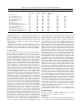
Measuring Latency in Virtual Environments
Sebastian Friston and Anthony Steed
Abstract—Latency of interactive computer systems is a product of the processing, transport and synchronisation delays inherent
to the components that create them. In a virtual environment (VE) system, latency is known to be detrimental to a user’s sense of
immersion, physical performance and comfort level. Accurately measuring the latency of a VE system for study or optimisation, is
not straightforward. A number of authors have developed techniques for characterising latency, which have become progressively
more accessible and easier to use. In this paper, we characterise these techniques. We describe a simple mechanical simulator
designed to simulate a VE with various amounts of latency that can be finely controlled (to within 3ms). We develop a new latency
measurement technique called Automated Frame Counting to assist in assessing latency using high speed video (to within 1ms). We
use the mechanical simulator to measure the accuracy of Steed’s and Di Luca’s measurement techniques, proposing improvements
where they may be made. We use the methods to measure latency of a number of interactive systems that may be of interest to the
VE engineer, with a significant level of confidence. All techniques were found to be highly capable however Steed’s Method is both
accurate and easy to use without requiring specialised hardware.
Index Terms—Latency, measurement
1
I NTRODUCTION
In the development of virtual environments (VEs), an important characteristic is latency. Defined as “the time lag between a user’s action...and
the system’s response to this action” [21], latency has repeatedly been
shown to reduce the effectiveness of virtual environments and other
interactive computer systems on many levels. Latency can result in a
discord between the proprioceptive cues of the user and the simulated
stimuli. This conflict between experienced sensations and expectations
learned over a lifetime results in reduced presence (the acceptance
of the virtual stimuli as real) [25]. Its impact in this respect has been
shown to be more significant than the difference between photo-real and
non-photorealistic rendering [31, 15], while other studies have found
it detrimental to performance in physical interaction [14], detrimental
to performance in collaborative tasks [7], and that it is responsible for
increased simulator sickness [4].
Those who have studied the effects of latency recommend VEs have
no more than 17ms [2] of effective delay, though others have found the
effects of latency at even lower levels [11]. Constructing a VE with
response times anywhere near these is difficult. Latency is a result of
the accumulation of processing and transport delays inherent to the
computer systems that constitute the VE. Further, measuring it is less
than straightforward. It is this last point, that we aim to address.
A number of authors have presented techniques for measuring latency, and they have become progressively easier to use with less
reliance on specialised hardware. Two of these techniques are Steed’s
Method, and Di Luca’s Method. Their simplicity, low cost and low coupling to the configuration of the VE under test make them applicable to
a wide range of interactive systems. The authors of those methods have
taken care to confirm their results against alternative systems where
available, but no objective characterisation of their accuracy exists. The
aim of this paper is to provide the VE engineer with a reference they
can use to select the most suitable measurement technique for their
situation, with awareness of the confidence they may have in the results.
In our study, the two techniques above are used to measure latency in
a controlled environment. In developing the test procedure, we create
a mechanical simulator capable of simulating the visual stimuli our
• Sebastian Friston is with University College London.
E-mail: [email protected]
• Anthony Steed is with University College London.
E-mail: [email protected]
Manuscript received 12 September 2013; accepted 10 January 2014; posted
online 29 March 2014; mailed on 1 May 2014.
chosen methods will expect, with finely controlled latency. In addition,
we develop an algorithm to perform frame counting automatically from
high speed video, which is presented here as a third alternative.
We begin with a review of latency measurement techniques, before
introducing our chosen techniques in detail, describing their operation
and what information about the accuracy can be inferred from the original publications. We describe the Automated Frame Counting method,
the motivation for machine-vision based automation of frame counting,
and present our automated counting solution. A mechanical simulator,
capable of simulating latency to within 3ms is documented and its
operation verified. Each measurement technique is used to estimate
latency from motion actuated by this simulator. We discuss the results,
investigating further where necessary to build an understanding of the
performance of the techniques under different conditions, and what
factors influence their accuracy. Finally, we use our results to characterise accuracies of the measurement techniques at a given confidence
interval, and use them to measure the latency of various real interactive
systems.
2
P REVIOUS W ORK
A number of latency measurement techniques have been developed.
Some observe the VE in action and attempt to monitor latency in the
same way it would be detected by the user. Others take advantage of,
or even modify, the VEs design in order to characterise it. Latency
measurement has been conducted on VEs from immersive acoustic
environments to those employing haptic feedback devices, but most
methods focus on assessing visual feedback [17, 9]. We continue this
trend as visual is the predominant stimuli in studies on the effects of
latency. In this section we review the various ways latency has been
measured in different interactive systems.
One way to characterise latency is to probe the connections between
the components (hardware or software) that combine to produce the
stimuli, assessing the delay of each stage individually. For example,
in their investigation into the delay of cloud gaming systems Chen et
al. hooked the EndScene() API of DirectX to ascertain the exact time
spent by the application drawing the scene [5].
Miller et al., in their investigation of an immersive acoustic environment, placed calls to toggle a pin on the parallel port at certain points
in the simulator software. These pins were monitored with an oscilloscope, along with output from the headphones and tracker hardware
[16]. This was also done by Mine, who externalised receipt of the tracking data when assessing the total end-to-end delay of a VE, through an
A/D converter [18]. This method provides good resolution. Miller, et
al, were able to identify the impact on delay of various output buffer
configurations, for example. However, it requires that the simulation be
modified at a low level, and the accuracy is dependent on the actuation
of the monitored events. In [1], Adelstein et al. measured how the
latency of trackers varied with different accelerations. The trackers
were attached to a mechanical arm fitted with a rotary encoder, which
provided the ground truth. A software library read the PC’s very precise
hardware timer directly, in order to determine the delays of each stage
in the communication paths between the encoder and tracker. In [16],
Miller et al. performed a loopback test to confirm the response times of
the parallel port used, but not all VE hardware may have this option.
The advantage of modifying the virtual environment system, is
that the scene is independent making it possible to gather comparable
performance data for varied virtual worlds. With VEs built from offthe-shelf modules, and modern operating systems further abstracting
the hardware, this is becoming more difficult. Perhaps as a result
most examples of measurement techniques are of the outside observer
type. Here, a latency measurement system passively monitors the real
and virtual world simultaneously and determines the latency from the
discrepancies between the observations. One advantage of outside
observer methods is that they assess the total time for the sensor data
to be acquired or output data to be actuated, which probing may miss.
Another is that they are independent of the VE implementation. An
example of this approach is by He et al., who monitored both a tracker
and an object within a VE, with a single camera. The latency was
derived by counting the frames between the movement of a real object
and corresponding movement of the virtual object (the manual frame
counting technique) [8].
Roberts et al., used the manual frame counting technique to measure
the end-to-end delay of an immersive collaborative environment using
synchronised cameras [22]. The frame counting technique is popular
because cameras are cheap and readily available. However it has
a number of drawbacks. The main drawback is that the resolution
of the measurement will be limited to no less than the length of 1
frame. If the exposure time of the camera is large enough with respect
to the frame rate of the output device, multiple output frames may
be captured resulting in ambiguity in when exactly the output event
occurred. All camera-based systems rely on the latency being higher
than the Nyquist rate of the camera, or no latency will be detected at all.
One way to negate these issues is to simply use a high speed camera,
though then the cost advantages diminish and due to the short exposure
time, illumination becomes a concern [30]. Alternatively, there are
techniques that derive latency independently of the frame.
Sielhorst et al., measured the latency of a video see-through AR
system by encoding times in moving circles on a display. A camera
recorded the display of the AR which contained both the true time and
time as visualised by the latent AR system. The latency could then be
‘read’ by decoding the timestamps from the positions of the circles. This
resulted in a resolution of 1ms [24]. Steed developed the Sine-Fitting
Method, where a camera monitored a (tracked) swinging pendulum and
a corresponding virtual pendulum. Image processing algorithms fit the
discrete locations of the targets from each frame on to two sine waves;
the phase difference between them can then be used to calculate the
latency. Steed obtained superior results to those achieved with a 500Hz
camera using the manual frame counting method [26]. Swindells et
al., superimposed a virtual turntable on top of a real one in a virtual
hand lab, and the latency was calculated from the angular difference
between the two [27]. These techniques allow for sub-frame length
resolutions. While they are all subject to motion blur or ‘bleeding’ of
the output frames, this has little effect on the results due to the choice of
image processing (Steed), encoding method (Sielhorst, et al) or capture
hardware (Swindells et al.). The methods are still subject to the Nyquist
rate however, and require constraints on the type of movement, and
composition of the VE.
Alternative techniques employ other capturing devices. Mine’s
method utilises photodiodes to detect the passing of a motion tracker
(attached to a pendulum) through a point, and a corresponding virtual
object through an equivalent location on the display [18]. This requires
the location of the photodiode on the display to be carefully calibrated
however. Di Luca presents a method where two photodiodes, one attached to a tracker, and one to the screen, move across two greyscale
gradients (one fixed relative to the moving tracker, the other virtual
moving with the aforementioned tracker fixed relative to the diode).
The signals output from the diodes are captured by the soundcard of a
computer, normalised, filtered and processed with a Fast Fourier Transform (FFT) to find the maximal frequencies (those corresponding to
the motion of the tracker); then as in Steed’s Sine-Fitting Method, the
phase shift determines the latency. The advantages of this method are
no calibration requirements (as only the change in gradient expressed
by each signal is considered) and the high sampling rate (potentially
44KHz) will be considerably higher than current displays [6].
All the methods so far have required some modification to the simulation software or hardware, or addition to the virtual scene. For example
Steed requires a scene containing a virtual pendulum while Di Luca
requires a gradient. A third type requires no modification to the VE at
all. An example of an entirely passive measurement is presented by
Miller and Bishop. Their technique, the latency meter, utilises 1D CCD
cameras (which can operate at much higher frequencies than regular
2D cameras) to identify the ‘centre of brightness’ of the scene they are
observing. Two synchronised cameras, one facing the (tracked) user,
the other the display of the VE, track the movement of this centroid
and calculate the latency from the difference between the two. Much
information is lost in this conversion of the scene to a 1D offset, and so
a linear relationship between the two centroids cannot be relied upon.
Instead Miller and Bishop use the velocity of the centroid (as when
the tracker is not moving, the VE should not change significantly),
matching ‘stop events’ between two signals and deriving latency from
the time between them. This technique, while not requiring explicit
modification of the VE, does rely on scenes where motion will result in
large changes in light levels. The technique was verified against Mine’s
method [16]. There is a limitation however that the technique shares
with all the aforementioned methods: it requires a sample of a number
of movements.
Wu et al., attempted continuous latency measurement with two
techniques: automated frame counting with a 1KHz camera, and an
angular difference method with a low frequency camera. For the frame
counting method, they implemented an algorithm that could identify
two frames temporally separated but in which the position of a slider
corresponded to the same location in both, this allowed continuous
measurement to 1ms resolution. For the angular difference method,
they implemented an algorithm which assessed the angle of two bars
and calculated the difference between them. Their measurements were
accurate enough to reconstruct the apparent oscillation of the latency
over time, due to the interplay between the different clocks of the
actuator and the sensor [30].
3
T HE S INE -F ITTING M ETHOD
The Sine-Fitting Method was introduced by Steed in 2008 in [26]. It is
an outside observer type technique that facilitates latency measurement
using commodity video cameras. With this technique, a salient object
within the VE is configured to follow a tracker. Both the tracker and the
object are captured in the same frame of low speed video, and machine
vision techniques used to recover their motion. By ensuring that the
tracker moves in a sinusoidal pattern, for example by attaching it to a
pendulum, sine waves can be fitted to the motions sampled at low rates.
The latency is then determined from the phase-difference between them,
at values much lower than the time between frames. Steed used the
Sine-Fitting Method to measure latency of different image generators
for a CAVE and an Intersense IS-900 tracker. The sinusoidal motion
was produced by attaching a tracker to a pendulum. Steed suggested
the method may be improved by using cross-correlation (personal
communication), which we investigate, so the method - measuring
latency from the phase difference of two cyclical motions sub-sampled
with low speed video - will herein be referred to as Steed’s method,
with two variants: sine-fitting and cross-correlation.
3.1
Implementation
In the reference implementation (based on code available from Steed1 ),
two targets of different colours are used.
1 Available
at http://www.cs.ucl.ac.uk/staff/ucacajs/LatencyDemo/
The video is cropped around each target resulting in two sequences.
For each, the median is calculated over the entire sequence and then
subtracted to remove the background. The sequence is then filtered on
the colour of the target to reduce the influence of noise. The horizontal
displacement of the target is then found by calculating the luminance
centroid for each frame.
Once the motion is extracted for each target, it is smoothed and
normalised to provide a set of samples characterising a sinusoid. A sine
wave is fitted to each set of samples with least-squares non-linear curve
fitting. This involves iterating to find the coefficients for a data-set,
that minimise the difference squared, with respect to a reference set.
In the Sine-Fitting Method, these coefficients are the frequency and
phase which define a sine-wave (the data set), and the reference set it is
compared with is the target motion.
The phase difference will be in fractions of a frame, and so knowing the framerate, the latency can be calculated to sub-frame length
accuracy.
3.2
Results
Steed compared the latency estimations of the method with the estimations obtained using manual frame counting and found them far
superior in resolution. The method was able to identify latencies of
11ms (between two eyes in frame sequential stereo video). An attempt
was also made to measure a difference of 3ms, being the difference
between different points of the scan out of CRT projectors. No statistically significant conclusion could be drawn from this, with the author
noting it could be due to limitations of the measurement technique or
inherent variations in the latency of the system.
4
D I L UCA ’ S M ETHOD
Di Luca developed the method presented in [6] in order to characterise
the effect of input frequency on VE latency. They note many techniques, including Steed’s Method, use pendulums, which oscillate at
only one frequency. The technique2 involves using two light-sensing
devices to capture the positions of the tracker, and an object in the
VE, synchronously. The tracker is attached to one device which moves
across a gradient, the virtual object is another gradient, which moves
in front of a static sensing device affixed to the display. The sensed
luminance is proportional to the horizontal displacement across the
gradient (position). The light-sensors are two photo-diodes, connected
to the input of a PC sound-card. The cost of the equipment is low, and
the sampling rates high. The tracker is moved in a roughly sinusoidal
pattern by hand, and the luminance/displacement measured by each
sensor captured. The waveforms are cross-correlated to determine the
delay.
4.1
Implementation
The light-sensing equipment consists of two photo-diodes, and amplifier circuits which are arranged such that a light-dependent voltage
source is provided by each. This is then connected to the input of an
A/D converter such as a sound-card. One concern with the use of a
soundcard is that it is likely to have a high-pass filter. As Di Luca notes
this is not usually an issue as the amplitude will be modulated by the
refresh rate of the display (nominally 60Hz). In practice however we
found that not all displays drive pixels black between frames. Displays
with LED backlights such as those in laptops for example, maintain a
constant luminance for unchanging visuals. In these cases it is necessary to reduce the brightness of the display and rely on the Pulse Width
Modulation (PWM) of the backlight to oscillate the illumination of the
entire screen.
Once suitable displays have been appropriated, standard audio
recording software can be used to capture the change in luminance
as the gradients move relative to their sensing devices. The samples
are then normalised and filtered in a number of steps to recover the
dominant waveform in each. The signals are first low-passed (10Hz) to
remove the modulating frequency that allows the signal to pass through
2 The
source code for the implementation
http://people.kyb.tuebingen.mpg.de/max/
is
available
at
the soundcard’s high-pass filter. They are then windowed to remove the
start and end periods. A Fast Fourier Transform is applied and from
this the dominant frequency (assumed to be the user’s movement) is
retrieved. The signals are then band-passed by convolving them with
a waveform of the dominant frequency. Now that the motions of the
tracker and virtual object have been recovered, cross-correlation is used
to identify the phase-shift between them.
4.2 Results
Di Luca did not compare the method’s results to those obtained with
another, but did modify the tracker configuration of the system under
test to introduce predictable amounts of latency and confirmed the
estimations responded appropriately. In one set of measurements a
standard deviation of 5.1ms was found, though again this is may be
inherent to the VE.
5 AUTOMATED F RAME C OUNTING
To compare the latency measurement techniques, we chose to characterise them by the error in their estimations. To determine error the
ground truth must be known. In our experiments the ground truth is
provided by a mechanical simulator, though in order to provide this,
its operation must be verified. To do this we elected to perform frame
counting. Manual frame counting as presented previously however
is not practical for the number of captures our investigation will involve, or the level of confidence we require, so we present here a new
algorithm to perform automated frame counting.
Frame counting involves capturing the system in operation, and
identifying the samples at which two tracked objects display common
and distinctive patterns of motion (such as starting and stopping, or
reaching a specific point in space). The number of samples between
them define the latency, in discrete units of time equivalent to the time
between samples. This method can be applied to almost any system
and, given an ideal capture, has a number of advantages including high
robustness and invariance, and the ability to measure changes in latency
during the capture.
In practice though, identifying where in the capture each event occurred is not straightforward. Given the small exposure times required
for such high capture rates, illumination becomes a concern [30, 26].
Lighting fluctuations or slight instabilities in the camera mount or the
tracked objects are manifested as small oscillations (noise) in the apparent position of the object in the video. As the frame rate increases the
distance an object can move between two consecutive frames decreases
until the difference between movement due to motion, and noise, becomes imperceptible. At 1000 fps if an object is moving fast enough
the SNR will be high enough to determine that the object is in motion,
but this highly limits the range of motions that can be detected, and
accelerations cannot be detected at all.
Wu et al., account for this by tracking the absolute normalised horizontal positions in space (instead of motion) and measure the latency by
identifying the frames at which the targets reach a specific offset from
the edge of the frame. This requires a perfect, known linear relationship
between the tracker and target position however. Wu et al., managed
this by using a video feed of the tracker as the actuator [30]. He et
al., measure a real system using a similar technique but with a grid for
guidance. Even with this though, and video captured at 60fps, they
report it took 10 hours to manually perform the frame counting and
suggest this process be automated with computer vision techniques [8].
5.1 Implementation of an automated frame counter
Our automated frame counting algorithm mimics the process of manual
frame counting: identify a distinctive pattern of motion, and then identify at which frame this began. Similar to Steed, and Wu et al., we use
image processing techniques to extract the horizontal positions of the
tracked objects throughout the capture, resulting in a set of samples (a
signal) that characterises the motion of the object. Identifying a distinctive pattern then becomes a problem of feature detection in the single
dimension. We nominate a motion feature with high distinctiveness
and localisation, and utilise feature detection algorithms to perform the
frame counting.
5.1.1 Capture setup
The setup for the Automated Frame Counting method is similar to
that of Steed, and Wu et al. A high speed camera is positioned to
capture both the tracker, and a virtual object, in the frame. The virtual
object should move in free space with the tracker. The algorithm
extracts foreground objects based on luminance, so the virtual object
and any marker attached to the tracker should be bright and distinctive
compared to the background. Once a capture of the targets in motion
has been taken, the algorithm will track their locations throughout the
video identifying distinctive motions, and when they occurred, for each
target.
5.1.2 Extracting motion from video
The signal we perform feature detection on is the set of horizontal
positions of a target over the entire capture. To extract these, the video
is filtered such that the background disappears and the targets remain
as solid clusters of pixels - binary blobs. The centroids of these are
then tracked throughout the sequence. First, each frame of the video is
grayscaled to get a single luminance value for each pixel. The histogram
of the first frame is then bi-segmented, clustering the luminance for
each pixel into one of two classes. All frames are binarised based on
one threshold. The user has the option to define the threshold. If they
choose not to, one is automatically calculated using Ostu’s method.
Ostu’s method selects a threshold such that the inter-class variance
of the luminances is minimised [20]. This method was selected as
it is simple and has been shown to be consistently among the better
performing thresholding methods [23].
Once all frames have been processed the user is presented with the
first frame again in order to nominate the positions of the objects to
track. For each frame in the sequence, all the binary blobs are identified.
For each object, the closest blob to the last known position is considered
to be the object in the current frame. The centroids are extracted and the
last known positions updated, and the process repeats on the next frame.
This heuristic is simple but due to the rate of capture is robust and
operates without the need for filtering or prediction. This method relies
on the assumption that the captures are taken of monochromatic targets
in environments with very little background noise. This is reasonable
because the algorithm was developed to assess latency measurement
techniques and throughout these experiments the environment can be
completely controlled. Should this be used to measure other VEs built
with a wide range of different hardware, the assumption is unlikely to
hold. A possible extension would be to replace the tracking of binary
blobs with that of image patches, which would allow this method to
measure VEs without any need to modify the scene, as any visually
distinctive object within it would suffice.
5.1.3 Extracting features from motion
Our algorithm operates by identifying a specific feature in motion. That
is, a pattern of displacements over time. We define the feature as the
peak of acceleration. This is the point at which the velocity is zero, as
the object changes direction in side-to-side motion. It was chosen as it
is highly salient, distinctive (the acceleration before and after is likely
to be high) and highly localised (the object will be still for smallest
amount of time permitted by the laws of physics) meeting much of the
criteria of the ideal local feature [28]. It also corresponds to the point in
a user’s motion that they are most likely to detect a discrepancy in the
simulated stimuli. Users are more sensitive to differences in velocity
than acceleration, so latency is most visible at the end of a movement
when the latent VE continues to a display fast moving stimuli relative
to the user’s quickly decelerating head or limb [10]. With this feature
the problem becomes that of edge detection in one dimension.
The detector must consider motion features (edges) with a large size
relative to that of an individual sample. The user’s speed will determine
how many samples their motion is completed within (the feature size),
and therefore a scale-invariant feature detector is required. We use
an edge detector introduced by Lindeberg which uses a first-order
Gaussian differentiating kernel applied at different scales, along with
an edge strength measure, to allow for automatic scale selection [12].
Our kernel is given by Equation 1, where s controls the width of the
function relative to the kernel scale and is defined as s = kernelscale ·
0.25 · widthscaling f actor.
g(x; s) =
−x −x22
e 2s
s2
(1)
The signal we convolve this kernel with is the set of positions of
our target over time. The result is the derivative of the signal, but
calculated for the total displacement over a set of samples, averaged
with a Gaussian function. The number of samples depends on the size
of the kernel. A Gaussian kernel was chosen as it was found by Canny
to be optimal in edge detection [19].
Averaging destroys local features which can be used to identify
the exact sample containing the peak of motion. To mitigate this,
we perform the convolution with functions of two different sizes as
demonstrated by Bao et al., based on the observation that as the scale
increases, noise is attenuated far more rapidly than the signal [3]. In
our implementation, the kernel size (scale) remains constant and the
width of the function is altered (with scaling factors of 1 & 0.5). The
product of the convolutions is a filtered signal which maintains high
locality while still permitting the algorithm to use averaging in order to
make the gradient a useful property for feature detection.
To extract features from this convoluted signal we use non-maximum
suppression as defined by Canny, selecting the sample at which the gradient assumes local maxima [29]. We define our own feature strength
measure which is based on the area under the potential feature. We
approximate the integral of this potential feature by summing the normalised magnitudes of the gradient at each sample within a window
centred on the feature. If this sum is within a range, the feature is
considered salient. The range is based on the shape of an ideal feature.
Its upper value is half the window, biased slightly to allow for nonideal waveforms. The window size and kernel scale are interdependent,
where the kernel scale is 4 · windowsize + 1.
To prevent the use of different scales on different targets introducing
error, a single scale which best represents the scale of the features
in both is chosen. This is done by performing the convolution for a
set of scales on each signal, and identifying the number of detected
features at each scale. The scales were selected so the window sizes
(∼10-1000 samples) spanned the periods of all the expected movement
frequencies (1-4Hz). The subsets for which the number of detected
edges is consistent between the two signals is extracted, and from these,
the set with the largest numbers of consecutive scales is identified. As
aliasing may cause the signal to resonate at multiple scales, the scale
set selection is guided by estimating the frequency (number of features)
based on zero crossings of the normalised signal.
The scale used to detect the edges is selected from near the end
of the set. Intuitively, the less averaging performed the better the
localisation, however we discovered in simulation that the error was
minimised when the scale was maximised, and the ideal scale is that
which approximates the size of the average feature. In the final stage,
the convolution is performed at this chosen scale on both signals, the
feature points extracted as described, and the latencies calculated by
subtracting the two feature point positions from each other.
This method of determining latency from the difference between
two discrete positions in time is similar to that of Wu et al., but where
they identify when each target reaches a specific displacement in space,
we identify when each achieves a maximal acceleration. This makes
fewer requirements of the VE as a linear spatial relationship between
the two targets is not needed.
5.2 Measuring latency with the automated frame counter
An implementation of the Automated Frame Counting method was
created. The user begins by selecting a viewpoint in the virtual world,
and positioning the tracker and camera as described in section 5.1.1.
Figure 1 shows an example of a suitable setup. In our experiments the
tracker was moved in a sinusoidal pattern for ∼3 seconds by hand.
The user provides our software with the video file. The software
guides them through selecting the threshold for binarising the frames,
and identifying the locations of salient objects to track. Once tracking is
complete the user selects the feature scale. To do this they are presented
Fig. 1. Example setup for the Automated Frame Counting method. The
mouse is the tracker and the VE is a Unity set.
with a plot of target positions. The features detected at the current scale
are indicated on the plot. The user increases or decreases the size of
the scale until the number and location of the detected edges matches
those suggested by the plot. The algorithm then extracts the features at
this scale. Subtracting the feature locations of one target from the other
provides the number of frames, and thus the latency, between them.
The average of these is returned as the latency estimate for that capture.
5.3 Verifying the algorithm
Pairs of sinusoidal waveforms were generated with sample rates equivalent to the frame rate of the high speed video, and Gaussian noise
introduced, at levels designed to mimic that encountered when recovering motion from the video. One of the sinusoids of each pair was
shifted to emulate latency. Waveforms of frequencies between 1-4Hz,
and latencies between 0-120ms were generated. The frame-counting
algorithm was then used to estimate the latency of the pairs. (From
here on in, simulated will refer to waveforms with controlled latency
but that have been recovered using the sensing devices & algorithms of
the aforementioned techniques, while virtual refers to those that have
been entirely procedurally generated to mimic them.)
5.4 Results & Failure Cases
The Automated Frame Counting algorithm estimates latencies between
corresponding motion features in the position samples of two targets
extracted from each capture. For each capture, a number of latencies
will be estimated, the number depending on the frequency of motion
and length of sample. For example, the virtual ‘captures’ all had lengths
of 3 seconds, so for motion at 1Hz, 6 estimations would be made. The
mean of these estimations is the estimated latency for that capture. This
figure is the one most comparable with the other techniques, all of
which estimate the average latency across the capture.
For each latency and frequency combination, three waveforms were
generated, the latencies estimated, and the error of these estimations
determined. The mean and standard deviation of these errors across
the three estimations are shown in Figure 2. The standard deviation
of the errors in the individual frame-to-frame latencies (the mean of
which defines the latency estimation for that capture) are also shown in
Figure 2, with diamond markers. For clarity, these data points show the
average across estimations for all frequencies at the given latency.
The least robust part of the algorithm is the automatic scale selection.
The reason for this is that it operates by first attempting to determine
the number of motion features in the video and then selects a scale
which resonates with this. This makes the scale selection more reliable,
but also makes assumptions about the characteristics of the features it
is trying to find that may not hold, especially for user generated motion.
The algorithm includes a stage after automatic scale selection, permitting manual verification and correction, it is recommended that this is
always used even if adjustment is rarely required. During verification
this was needed even with the perfect sinusoids, as in some virtual
waveforms the randomly generated noise was significant enough to
confound the feature count estimation.
Another likely source of error is in the latency estimation stage.
This occurs after feature location extraction, and during which the
feature locations from one waveform are subtracted from the other.
This simplistic method does not ensure the motion feature locations
being subtracted correspond and it is therefore possible to subtract the
wrong locations from each set. This may occur if a feature is detected
in the latent signal, before the first feature in the primary signal, for
example. This again can be avoided by verifying the detected features
in the scale selection stage.
Finally, the object tracking algorithm has a limitation where if a
tracked object is not visible in a frame, it will lose it for the remainder of the sequence and begin tracking another target - possibly the
counterpart leading to erroneous latency estimations of zero. This can
occur for example on displays which use Cold-Cathode Fluorescent
Lamp (CCFL) back-lights or those with LEDs utilising PWM to control
the brightness. This limitation needs to be corrected by using a more
sophisticated algorithm that will take the entire sequence into account
as it severely limits the applicability of this technique to real systems.
For this investigation latency estimations were done on systems using
CRT displays, or LED backlit displays with the brightness set to 100%.
Once the correct scale has been identified however the algorithm
is highly reliable. Out of over 2000 individual latency estimations
performed on virtual waveforms, the largest deviation from ground
truth was 4ms. The mean of a set of estimations will characterise the
latency to under 1ms with a CI (confidence interval) of 99% (calculated
from the estimations of all latencies for all frequencies with a Critical
(Z) Value of 2.58).
5.4.1
1 Hz
2 Hz
3 Hz
4 Hz
Estimation Error Mean &
Standard Deviation (ms)
2
1.5
1.5 Hz
2.5 Hz
3.5 Hz
1
0.5
0
−0.5
0
1
5
15
30
Virtual Latency (ms)
60
120
Fig. 2. The error in the estimates of latency in virtual waveforms made
by the Automated Frame Counting method, for a range of latencies and
frequencies
Characterisation Metric
To characterise and compare the measurement techniques, we chose
to use the confidence interval of the estimation error at 99%. Given a
population, such as a set of estimation errors, this metric determines a
range that any future member of the population will fall within, with a
given probability, based on previous observations. By calculating the
CI in terms of estimation error, we define the error margin that an end
user can expect for their measurement with a high level of confidence.
This is an intuitive characterisation of accuracy that can be used to
compare the techniques. Throughout our experiments we determined
estimation error for a range of frequencies and latencies so that any
interaction between these variables and accuracy could be detected.
The CI was always calculated in the same way, from the complete set
of these, to ensure the characterisations are applicable under a wide
range of conditions and directly comparable.
6
M ECHANICAL L ATENCY S IMULATOR
To measure the accuracy of latency measurement techniques, we created a mechanical simulator which would mimic an interactive system
as seen by the ‘outside observer’ camera, using targets actuated by mechanical devices, the latency of which could be finely controlled. Two
Hitec HS-303 RC Servos were connected to an FPGA development
board. RC Servos are driven by a 50Hz PWM signal where the Ton
period defines the angular offset of the servo’s shaft from its neutral position. The servos we used supported a duty cycle of 1500-1900µs for
a range of 90◦ . Our system accepted position samples from a desktop
computer and used them to define the duty cycle of the signal transmitted to the servos. This signal could be delayed for one servo, by a
set amount of time, or as a function of time, by sending delay samples
from the desktop. Delaying the waveform was achieved by sampling it
at 256KHz, converting it into a 1 bit data stream, which was fed into a
FIFO buffer. The stream received by the servo was not the output of
the buffer but a specific offset into it. The size of this offset determined
the delay, and allowed the delay to be decreased instantaneously at any
point during the simulation. 256KHz results in a period of 4µs which
is well within the deadband of the servos used (that is, the resolution
of the change in duty cycle that would cause the servos to move). By
using an FPGA the control system for the servo could operate at far
higher rates than one driven directly by a PC, permitting very high
resolutions. Our control system is similar to that of Adelstein et al.,
designed to actuate trackers with varying frequencies and amplitudes
using a mechanical arm. In their system a motor controller configured
a function generator, which drove a DC motor with smoother sinusoids
than the motor controller itself was capable of generating [1]. Servos
operate by using a potentiometer as a rotary encoder and drive a DC
motor connected to the shaft through a gearing system back or forth to
match the intended rotation based on the impedance of the potentiometer. Therefore, servos are more vulnerable to manufacturing tolerances
and wear than other options such as stepper motors. Out of four servos,
only two had performance characteristics similar enough to actuate the
targets with a temporal resolution of 1ms. If an equivalent mechanical
simulator is built it may require the designer to try multiple servos, or
perform calibration.
Estimation Error Mean &
Standard Deviation (ms)
6.1 Verification
The mechanical simulator was used to actuate sinusoids between 1-4Hz
at latencies between 0-120ms. The latency was estimated with the
Automated Frame Counting method. The motion for each combination
was repeated three times.
1 Hz
2 Hz
3 Hz
3
1.5 Hz
2.5 Hz
4 Hz
2
7
R ESULTS
The mechanical simulator described above was used to simulate user
motion and latent feedback, at frequencies of 1-4Hz with delays of
0-120ms. In all simulations performed to assess the techniques, high
speed video (1000fps) was taken to verify simulator operation. For
each combination of frequency & latency, the targets were oscillated
for three seconds, three different times. The latency was estimated for
each of these and the error (the deviation from the simulated latency)
calculated. Any time the estimation error of a technique under test
rose above 3ms (the level of confidence we have in the mechanical
simulator) the high speed video was reviewed. At no time did this show
an error was due to incorrect simulator operation.
7.1
Steed’s Method
To assess the accuracy of Steed’s method, the mechanical simulator
was fitted with two glossy targets. The motions were captured with a
Panasonic HD camcorder at 25fps.
The Sine-Fitting Method was modified, replacing the region centroid
based tracker with the binary blob based tracker used in the Automated
Frame Counting method. Reviewing the horizontal motions recovered
with each method had revealed the blob based tracker had less noise
and jitter. Steed suggested the method may be improved by using crosscorrelation, in place of sine-fitting with least squares. Without requiring
the movement to emulate a perfect sinusoid this is more tolerant of
discontinuities in movement, frequency and of quantisation noise (in
the time domain). The code provided by Steed was modified to perform
latency estimation using both sine-fitting and cross-correlation so that
they could be compared.
Video was captured at a resolution of 1920x1080. This was then
down-sampled and the measurements (including tracking) repeated
at 960, 480 and 240 lines to check the significance of the effects of
(spatial) quantisation noise. Initial results suggested an interaction
between spatial resolution and accuracy for both methods (Table 1), and
movement frequency and accuracy for the sine-fitting variant (Table 2).
Table 1 shows the mean, standard deviation, maximum and minimum
error in all estimations for all frequencies and latencies performed at the
displayed resolution. Table 2 shows the mean and standard deviation for
all latency and resolution combinations, for each movement frequency.
Table 1. Estimation error of simulated latencies with Steed’s method at
various resolutions
Resolution (lines)
Error (ms)
Mean
1
0
−1
0
1
5
15
30
Actuated Latency (ms)
60
120
1920
960
480
240
11.67
3.99
6.09
7.22
1920
960
480
240
7.76
2.06
2.21
1.98
Standard Deviation
Sine-Fitting Method
10.19
6.46
8.83
10.95
Cross-Correlation
3.96
1.66
1.49
1.36
Minimum
Maximum
0.18
0.01
0.09
0.04
85.09
72.16
10.00
12.92
0.00
0.00
0.00
0.00
22.00
9.00
8.00
1.00
Fig. 3. The actuation error of the mechanical simulator measured with
the Automated Frame Counting method for a range of latencies and
frequencies
7.1.1
Figure 3 shows the mean and standard deviation of the actuation
error. The standard deviations for frame-to-frame latencies within each
capture are again averaged for each frequency and illustrated with
diamond markers.
The maximum error out of all estimations in all captures was 8ms.
For a set of oscillations over a three second period, we can simulate
latency on average to within 3ms with a confidence interval of 99%
(calculated from estimations of all latencies for all frequencies, with a
Critical (Z) Value of 2.58 (∼2ms), including possible estimation error
of the Automated Frame Counting method (1ms)).
From Table 1 we can see the results are consistent for cross-correlation
for all frequencies and resolutions, with the exception of 1920x1080
which shows a marked decrease in accuracy. That the other resolutions
show no interaction with accuracy suggests that this is due to the object
tracking rather than position resolution. The recovered positions for
videoed targets at 1920 and 960 were taken and quantisation noise
introduced by dividing the displacement samples and rounding down.
The latency was estimated for a number of divisors.
Figure 4 illustrates the influence of spatial quantisation noise. The
plots show the sum of the mean error and one standard deviation so
neither metric can provide a false sense of confidence. The error and
Steed’s Method: Spatial Resolution & Accuracy
Error (ms)
Error Mean & Standard
Deviation Sum (ms)
Mean
Standard
Deviation
35
30
25
20
15
10
5
0
1.5
3.86
4.60
4.84
7.40
0.59
0.50
Cross-Correlation
1.63
2.70
2.46
1.30
1.29
1.49
Sine-Fitting
3.13
3.66
7.94
18.05
4
Varying
9.05
11.83
2.19
1.81
200
100
150
50
Movement Spatial Range (resolution) (Pixels)
0
Fig. 4. The sum of the mean and one standard deviation of the estimation
error for all latencies and frequencies, for estimations performed at
various video resolutions by Steed’s method
standard deviation, the sum of which is shown, are the mean of those
calculated for all six latencies, when oscillating at 2Hz. The tracked
positions from two captures were divided, the first captured at 1920
lines, the other at 960. For each capture, the divisor was increased by
the power of two each step until the range became so small latency
estimation could not be completed.
Figure 4 demonstrates that spatial resolution has little impact on
the accuracy of the estimations. A spatial resolution of as little as 20
pixels is sufficient to recover the latency to within 6ms (CI 99%). Both
sine-fitting with least-squares and cross-correlation have a minimum
resolution below which they are unable to reliably recover the latency,
cross-correlation has a slightly lower threshold.
From Tables 1 & 2 we can see that cross-correlation has consistently higher accuracy than sine-fitting with least-squares. Table 2 also
suggests that the Sine-Fitting Method may be less reliable at higher
frequencies, possibly due to temporal quantisation noise.
7.1.2
300
200
1 Hz
1.5 Hz
2 Hz
2.5 Hz
3 Hz
3.5 Hz
4 Hz
100
0
5 10 15 20 25 30 40 50 75 100 125 300 5001000
Frame Rate (fps)
Fig. 5. Mean estimation error of the sine-fitting variant over all latencies, at all frequencies, for estimations performed on videos of various
framerates
Sine Fitting 1920
Cross-Correlation 1920
Sine Fitting 960
Cross Correlation 960
250
400
2.95
2.62
Steed’s Method: Temporal Resolution & Accuracy
To investigate how temporal resolution could affect the accuracy of
the estimations, pairs of waveforms at frequencies between 1-4Hz
where generated with rates of 1000 samples/s, with the same latencies
(0-120ms) as used in previous tests. These were then subsampled to
emulate captures at framerates between 5 and 1000fps.
Figures 5 & 6 show how the mean error of both estimation methods
vary with framerate, for a set of seven frequencies (again, these are the
errors over a number of latencies from 0 to 120ms). In both cases the
the accuracy is invariant of the framerate until it is a low enough value
such that the motion cannot be accurately expressed and estimation
fails. This value is frequency dependent. Again cross-correlation
demonstrates more consistent and higher accuracy.
By introducing spatial quantisation noise above, we have shown that
not only is accuracy invariant with spatial resolutions above a certain
threshold, but that this threshold is considerably small. Therefore high
speed video can be used to verify the interaction of temporal resolution
and accuracy. The high speed video was subsampled by extracting
Estimation Error Mean (ms)
Mean
Standard
Deviation
Frequency
2
3
1
Estimation Error Mean (ms)
Table 2. Estimation error of simulated latencies with Steed’s method at
various frequencies
30
1 Hz
1.5 Hz
2 Hz
2.5 Hz
3 Hz
3.5 Hz
4 Hz
20
10
0
5
10 15 20 25 30 40 50 75 100 125 300 5001000
Frame Rate (fps)
Fig. 6. Mean estimation error of the cross-correlation variant over all
latencies, at all frequencies, for estimations performed on videos of
various framerates
frames at set intervals, to provide the Sine-Fitting Method with higher
rate captures at 3 & 4Hz. Corroborating the results from our virtual
data, the accuracy of cross-correlation remained unaffected, and the
estimations from sine-fitting were not improved.
Since the noted error at higher frequencies is not a result of framerate,
and does not occur in the estimations of virtual waveforms or in the
estimations using cross-correlation, we conclude it is a result of the
imperfections of the actuated waveforms, in which the sinusoid appears
to skew slightly as the servos are driven towards their limits by the high
rates of motion which confounds the sine-fitting process.
We also subject both methods to a waveform consisting of a set of
sequential single cycles at increasing frequencies, to emulate how a
user’s manual motion may vary in speed. As expected the least-squared
fitting function is unable to resolve to a single frequency.
Figure 7 shows the mean, and standard deviation of the errors, for
the various combinations of frequency and mechanically simulated
latency. The figures are averaged for all resolutions except 1920, the
results of which were considered invalid. The plot does not display
the estimations made by the Sine-Fitting variant of the 4 Hz or varying
waveforms. The cross-correlation variant results are shown by the solid
lines, while those of the sine-fitting variant are shown by dashed lines.
Each frequency/latency combination was simulated three times, and
the standard deviation shown is of the estimations for these three.
7.1.3 Steed’s Method: Conclusions
We have demonstrated that Steed’s method, both the sine-fitting and
cross-correlation variants, can have accuracies as high as ∼12ms and
∼7ms respectively (best-case CI of 99% when the tracked motion is
perfectly sinusoidal). When testing the interaction of resolution (spatial
range) and accuracy we encountered anomalous results. Investigating
this interaction further however revealed no relationship between this
variable and accuracy of the estimation algorithm. Instead the algorithm
was proved to be highly robust to quantisation noise in the time and
1 Hz Cross Correlation
2 Hz Cross Correlation
4 Hz Cross Correlation
1 Hz Sine Fitting
2 Hz Sine Fitting
Estimation Error Mean &
Standard Deviation (ms)
30
1.5 Hz Cross Correlation
3 Hz Cross Correlation
Varying Cross Correlation
1.5 Hz Sine Fitting
3 Hz Sine Fitting
Table 3. Estimation technique accuracy (ms) with a 99% CI
Estimation Error Characteristic (ms)
Characteristic
Method
Automated
Frame Counting
0.23
0.21
0.00
1.17
Steed
Di Luca
Mean
Standard Deviation
Minimum
Maximum
Mechanical
Simulator
0.64
0.47
0.00
2.00
2.08
1.79
0.00
9.00
2.79
1.90
0.00
9.00
Accuracy at 99% CI
1.86
0.78
6.69
7.68
20
10
0
7.3
0
1
5
15
30
Actuated Latency (ms)
60
120
Fig. 7. The error in the estimations made by both variants of Steed’s
method, for multiple latencies and frequencies
spatial domains, and we determined guideline minimums for both. The
anomalous results are likely due to errors introduced by the tracking
code. The cross-correlation variant has proven to be significantly more
reliable and consistent in its performance than sine-fitting using leastsquares so this variant will be used henceforth.
7.2
Di Luca’s Method
To assess Di Luca’s Method the capturing hardware was built as described and the diodes attached to the arms that actuated the targets in
prior simulations. These were placed against an LCD display showing
a single gradient. The arms were side by side as before so each diode
viewed a distinct horizontal section of the gradient.
The arms were actuated at frequencies between 1-4Hz, with latencies
between 0-120ms. Di Luca’s Method includes stages to allow manual
correction of the derived dominant frequency and correlation, however
we found no corrections were needed. The errors in the estimations
(mean and standard deviation) are displayed in Figure 8.
1 Hz
1.5 Hz
2 Hz
2.5 Hz
3 Hz
4 Hz
Varying
Estimation Error Mean &
Standard Deviation (ms)
10
8
(No Bandpass)
(No Bandpass)
(No Bandpass)
(No Bandpass)
(No Bandpass)
(No Bandpass)
(No Bandpass)
6
4
2
0
0
1
5
15
30
Simulated Latency (ms)
60
120
Fig. 8. The error in the estimations made by Di Luca’s Method, for
multiple latencies and frequencies
Computing the error mean (2.8ms) and standard deviation (1.9ms)
for all latencies, for all frequencies allows us to determine an accuracy
of ∼8ms with a CI of 99% for this method.
Summary
Table 3 attempts to illustrate the confidence one may have in any
technique or the mechanical simulator. The figures were calculated
from the set of error values for all latencies and all frequencies for
each method. Error values are defined as the absolute deviation from
ground truth (the simulated value). The error values for the mechanical
simulator entry were measured with the Automated Frame Counting
method. The values for the Automated Frame Counting method were
calculated from estimations performed on virtual waveforms. For
Steed’s method the figures for all resolutions were included, except for
the 1920 line captures which were considered invalid. The confidence
interval was calculated with a Critical (Z) Value of 2.58.
8
T HE
MEASURED LATENCY OF REAL SYSTEMS
After benchmarking the methods we attempted to determine how their
estimations compared when measuring real interactive systems. We
selected a set of systems chosen to represent both a range of interaction
paradigms for which latency is important, and a range that will have
high variance in performance.
The results are summarised in Table 4. For the Automated Frame
Counting method, the maximum & minimum latencies from the set of
estimations for a given capture are included to illustrate the variations in
latency of real systems. In addition to frame counting, cross-correlation
was performed on the recovered positions from the high speed video.
This further confirmed our findings into the invariance of accuracy with
temporal resolution, as the differences between these results and those
of Steed’s method are marginal and within measurement error.
As evidenced by the range determined by Automated Frame Counting, real VEs, especially those running on PCs which are tasked with
other concurrent responsibilities, are highly complex, and a great number of factors will determine performance. The measurements in Table
4 have been performed in sets designed to illustrate the performance
impact that may be expected from changing one parameter of various
configurations. It should not be considered as an accurate characterisation of the absolute performance of any of the included components or
technologies. When considering the maximum & minimum latencies
for a given measurement it is also worth recalling that the automated
frame counting estimation (for which the confidence interval in Table
3 is calculated) is the mean of the set of estimations. Larger errors
may be encountered within that set (up to 4ms was found during the
verification stage).
In some configurations (*), a gradient could not be made available
for Di Luca’s Method, so results for these are not present. In another
configuration (**), we used a Bluetooth tracker which was designed
to control the cursor with pointing motions and therefore the mapping
between lateral physical movement and motion on screen made it
difficult to capture the tracker with a gradient. This is a limitation of
our code, not Di Luca’s Method, so although a result was derived it
was considered invalid and omitted.
For the tests on Desktop 1, two demonstrations were built that displayed a white circle or gradient moving with the input device. One
used a PictureBox control on a Winforms application, the other displayed a textured quad in an OpenGL (SharpDX) viewport. Both were
written in C# using .NET. For the Unity measurements, an environment
containing a textured plane was created. The prefabs included in the
Table 4. Latencies of interactive computer systems estimated with various methods
System
PC 1 Mouse Aero On
PC 1 OpenGL Windowed Aero On
PC 1 OpenGL Windowed Aero Off
PC 1 OpenGL Full Screen Aero On
PC 1 OpenGL Full Screen Aero Off
PC 1 Winforms Aero On
PC 1 Winforms Aero Off
PC 1 Winforms Bluetooth Tracker Aero Off
PC 1 Winforms RAT5 Gaming Mouse Aero Off
PC 2 Unity Oculus Rift Tracker Aero Off
PC 2 Unity Mouse Aero Off
PC 3 OptiTrack Arena Raw Targets Aero Off
PC 3 OptiTrack Motive Raw Targets Aero Off
PC 3 OptiTrack Motive Rigid Body Aero Off
Latency Estimate (ms)
Automated Frame Counting Method
Mean Latency
Maximum
Minimum
Cross-Correlation
(1000fps)
30.00
45.00
11.00
29.00
58.78
64.00
53.00
52.00
24.00
32.00
18.00
22.00
49.83
60.00
23.00
45.00
24.00
33.00
13.00
22.00
58.47
66.00
50.00
53.00
34.64
44.00
29.00
31.00
30.27
39.00
17.00
22.00
26.56
36.00
22.00
17.00
27.27
50.00
14.00
25.00
87.46
96.00
78.00
83.00
55.00
60.00
51.00
40.00
52.00
56.00
46.00
43.00
50.43
54.00
46.00
48.00
Oculus Rift SDK were used to control the camera, and modified to support input from the mouse, so the same configuration is used for both
the mouse and Rift tracker measurements. The measurements of the
OptiTrack system were taken from the preview window of the included
software (Arena 1.8.6 & Motive 1.0.1) and include the rendering time
of that application.
It has been asserted that the Aero feature of Windows Vista and 7,
can introduce a frame of delay [13]. We found this was the case for
both Winforms, and OpenGL applications, windowed and full screen,
with Aero introducing ∼20ms of latency with a refresh rate of 60Hz.
9
C ONCLUSIONS
Latency is of high concern to those who engineer virtual environments.
We have investigated and demonstrated the accuracy of two measurement methods, both of which are easy to use and compatible with a
wide range of VEs. Both methods operate by sensing motion, resulting
in signals which describe the change in position of targets over time.
The phase shift that minimises the difference between these defines the
latency. By cross-correlating virtual waveforms of various frequencies
and phases, we have shown high invariance with low spatial (20 pixels)
and temporal (25 fps) resolutions. This suggests that the predominant
source of estimation error will be spatial error in the recovered motion
from the sensing devices or their pre-processing algorithms. We constructed a mechanical simulator of which the latency could be finely
controlled, and used it to investigate Steed’s Method using cameras,
and Di Luca’s Method using photodiodes. Both were found to be highly
accurate. Subsampling the captures taken for Steed’s Method in the
spatial domain reinforced what we found with virtual data - that spatial
resolution has no significant interaction with accuracy. Given this, we
subsampled low resolution (224x64) high speed video in the temporal
domain and found again the empirical measurements corroborated what
we found with virtual data. In order to verify operation of the mechanical simulator the Automated Frame Counting method using high speed
video was used. In theory the latency is directly observable with discrete frames and the accuracy is unquestionable when frame counting.
In practice we discovered what others had found in that manual frame
counting is time consuming and far from error free due to the difficulty
in determining motion from noise. Consequently, we present an automated frame counting method based on image processing techniques
(blob tracking and edge detection). We prove the concept with virtual
data, and verify the operation of the mechanical simulator and the
method in practice through demonstrating the high correlation between
intended latency and estimated latency when both operate together. We
present this method as a third latency measurement technique, with the
advantage that it can measure changes in latency over relatively small
amounts of time. If we consider the worst case 99% CI mechanical simulator actuation (∼2ms) + automated frame counting estimation error
(∼1ms), we could state with confidence the Automated Frame Counting
Steed’s Method
Di Luca’s Method
32.00
51.00
22.00
44.00
21.00
51.00
32.00
23.00
21.00
26.00
80.00
40.00
43.00
46.00
*
61.00
23.00
47.00
12.00
40.00
22.00
**
21.00
35.00
87.00
*
*
*
method has an accuracy of ∼3ms. This is similar to the average 99% CI
across the various frequencies under test, for Steed’s Method (∼7ms)
and Di Luca’s Method (∼8ms). With these levels of confidence we
measure a number of interactive systems. We find as expected the
cross-correlation of motion from video, at 1000fps and 25fps results in
deviations in the estimations of a few ms (within measurement error),
and these estimations correlate strongly with the average latency estimated using Automated Frame Counting. Di Luca’s Method deviates
further from the latency estimated by Steed’s method, but is generally
within the range found by the Automated Frame Counting method,
suggesting it tends towards one extreme or the other (or perhaps the
latency encountered during the movement at the dominant frequency
the algorithm band-passes on). Automated Frame Counting demonstrated the highest accuracy, but capturing VEs with high-speed video
introduced complications not found with the low-speed video used in
Steed’s Method. For example, the low resolution required the tracker
to be physically close to the display, and the tracked object in the scene
be larger than would have normally been necessary. Additional lighting
was also needed. With a suitable object tracking algorithm, both Automated Frame Counting and Steed’s Method could operate without any
modification to the VE, as they would be capable of tracking existing
salient objects within a scene. The objects and environments to which
they apply however are limited. To be suitable a target object must be
free in space with a linear relationship between its acceleration and that
of the tracker. If the VE alters the behaviour of the object in any way
(e.g. damping its movement, or altering its trajectory due to it colliding
with another object in the scene) the latency measurement would be
inaccurate. Di Luca’s Method’s specialised hardware makes demands
of the display technology and scene that camera-based methods do not.
It also overcomes limitations inherent to these methods. It may be the
only applicable technique when, for example, the tracker and display
are physically far apart, the tracker is not visibly salient, or items in the
scene cannot be reliably tracked (as we have already encountered).
In conclusion, any of the three latency measurement methods could
accurately characterise the latency of a VE. We found Steed’s Method
to be easiest to use however, and the gains in accuracy provided by
more specialised hardware to be no greater than the inherent variations
found in most of the real systems above.
The manuals & modified source code for all techniques and the
mechanical simulator can be found at www.cs.ucl.ac.uk/staff/s.friston/.
ACKNOWLEDGMENTS
The authors would like to thank Dr. William Steptoe for his help
measuring the latency of a number of VE systems.
R EFERENCES
[1] Bernard D. Adelstein, Eric R. Johnston, and Stephen R. Ellis. Dynamic Response of Electromagnetic Spatial Displacement Track-
ers. Presence (Cambridge, Mass.), 5(3):302–18, 1996.
[2] Bernard D. Adelstein, Thomas G. Lee, and Stephen R. Ellis. Head
Tracking Latency in Virtual Environments: Psychophysics and
a Model. Proceedings of the Human Factors and Ergonomics
Society Annual Meeting, 47(20):2083–2087, October 2003.
[3] Paul Bao, Lei Zhang, and Xiaolin Wu. Canny Edge Detection Enhancement by Scale Multiplication. IEEE transactions on pattern
analysis and machine intelligence, 27(9):1485–90, September
2005.
[4] Timothy J. Buker, Dennis A. Vincenzi, and John E. Deaton. The
Effect of Apparent Latency on Simulator Sickness While Using
a See-Through Helmet-Mounted Display: Reducing Apparent
Latency With Predictive Compensation. Human Factors: The
Journal of the Human Factors and Ergonomics Society, 54(2):235–
249, January 2012.
[5] Kuan-Ta Chen, Yu-Chun Chang, Po-Han Tseng, Chun-Ying
Huang, and Chin-Laung Lei. Measuring the latency of cloud
gaming systems. Proceedings of the 19th ACM international
conference on Multimedia - MM ’11, page 1269, 2011.
[6] Massimiliano Di Luca. New Method to Measure End-to-End
Delay of Virtual Reality. Presence, 19(6):569–584, December
2010.
[7] Chris Gunn, Matthew Hutchins, and Matt Adcock. Combating
Latency in Haptic Collaborative Virtual. Presence, 14(3):313–
328, 2005.
[8] Ding He, Fuhu Liu, Dave Pape, Greg Dawe, and Dan Sandin.
Video-Based Measurement of System Latency. International
Immersive Projection Technology Workshop, 2000.
[9] Caroline Jay, Mashhuda Glencross, and Roger Hubbold. Modeling the effects of delayed haptic and visual feedback in a collaborative virtual environment. ACM Transactions on Computer-Human
Interaction, 14(2):8–es, August 2007.
[10] Jason Jerald, Tabitha Peck, Frank Steinicke, and Mary Whitton.
Sensitivity to scene motion for phases of head yaws. In Proceedings of the 5th symposium on Applied perception in graphics and
visualization - APGV ’08, page 155, New York, New York, USA,
2008. ACM Press.
[11] Jason J Jerald. Scene-Motion- and Latency-Perception Thresholds
for Head-Mounted Displays. PhD thesis, University of North
Carolina at Chapel Hill, 2010.
[12] Tony Lindeberg. Edge Detection and Ridge Detection with Automatic Scale Selection. International Journal of Computer Vision,
30(2):117–154, 1998.
[17] Joel D. Miller, Mark R. Anderson, Elizabeth M. Wenzel, and
Bryan U. McClain. Latency measurement of a real-time virtual
acoustic environment rendering system. Proceedings of the 2003
International Conference on Auditory Display, Boston, MA, 6-9
July 2003, 2003.
[18] Mark R. Mine. Characterization of end-to-end delays in headmounted display systems. Technical report, University of North
Carolina at Chapel Hill, 1993.
[19] Mark S. Nixon and Alberto S. Aguado. Feature Extraction and
Image Processing. Newnes, 2002.
[20] Nobuyuki Otsu. A Threshold Selection Method from Gray-Level
Histograms. IEEE Transactions on Systems, Man, and Cybernetics, 9(1):62–66, 1979.
[21] Giorgos Papadakis, Katerina Mania, and Eftichios Koutroulis. A
system to measure, control and minimize end-to-end head tracking latency in immersive simulations. VRCAI ’11 Proceedings of
the 10th International Conference on Virtual Reality Continuum
and Its Applications in Industry, pages 581–584, 2011.
[22] David Roberts, Toby Duckworth, Carl Moore, Robin Wolff, and
John O’Hare. Comparing the End to End Latency of an Immersive
Collaborative Environment and a Video Conference. 2009 13th
IEEE/ACM International Symposium on Distributed Simulation
and Real Time Applications, pages 89–94, 2009.
[23] Mehmet Sezgin and Bulent Sankur. Survey over image thresholding techniques and quantitative performance evaluation. Journal
of Electronic Imaging, 13(1):220, January 2004.
[24] Tobias Sielhorst, Wu Sa, Ali Khamene, Frank Sauer, and Nassir
Navab. Measurement of absolute latency for video see through
augmented reality. 2007 6th IEEE and ACM International Symposium on Mixed and Augmented Reality, pages 1–4, November
2007.
[25] Mel Slater, Beau Lotto, Maria Marta Arnold, and Maria V
Sanchez-Vives. How we experience immersive virtual environments: the concept of presence and its measurement. Anuario de
Psicologı́a, 40(2):193–210, 2009.
[26] Anthony Steed. A Simple Method for Estimating the Latency
of Interactive, Real-Time Graphics Simulations. Proceedings
of the 2008 ACM symposium on Virtual Reality Software and
Technology, pages 123–129, 2008.
[27] Colin Swindells, John C Dill, and Kellogg S Booth. System lag
tests for augmented and virtual environments. In Proceedings of
the 13th annual ACM symposium on User interface software and
technology - UIST ’00, pages 161–170, New York, New York,
USA, 2000. ACM Press.
[13] Joe Ludwig. Lessons learned in porting Team Fortress 2 to Virtual
Reality. Game Developers Conference, 2013.
[28] Tinne Tuytelaars and Krystian Mikolajczyk. Local Invariant Feature Detectors: A Survey. Foundations and Trends in Computer
Graphics and Vision, 3(3):177–280, 2007.
[14] I. Scott MacKenzie and Colin Ware. Lag as a determinant of
human performance in interactive systems. In Proceedings of
the SIGCHI conference on Human factors in computing systems
- CHI ’93, pages 488–493, New York, New York, USA, 1993.
ACM Press.
[29] O. R. Vincent and O. Folorunso. A descriptive algorithm for sobel
image edge detection. Proceedings of Informing Science & IT
Education Conference (InSITE), 2009.
[15] Michael Meehan, Sharif Razzaque, Mary C. Whitton, and Frederick P. Brooks Jr. Effect of latency on presence in stressful virtual
environments. Proceedings of the IEEE Virtual Reality 2003,
2003:141, 2003.
[16] Dorian Miller and Gary Bishop. Latency meter: a device endto-end latency of VE systems. Electronic Imaging 2002, pages
458–464, 2002.
[30] Weixin Wu, Yujie Dong, and Adam Hoover. Measuring Digital
System Latency from Sensing to Actuation at Continuous 1-ms
Resolution. Presence: Teleoperators and Virtual Environments,
22(1):20–34, 2013.
[31] Paul Zimmons and Abigail Panter. The Influence of Rendering
Quality on Presence And Task Performance in a Virtual Environment. Proceedings of the IEEE Virtual Reality 2003, pages
293–294, 2003.