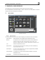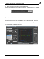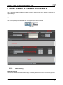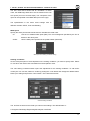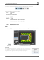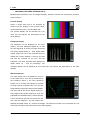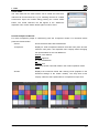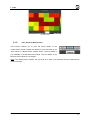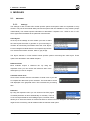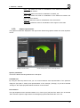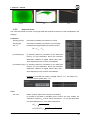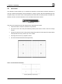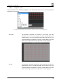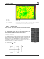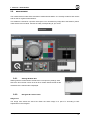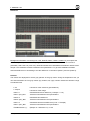
1
iQ-ANALYZER User Manual 26 August 2014 Image Engineering GmbH & Co. KG . Augustinusstraße 9d . 50226 Frechen . Germany T +49 2234 995595 0 . F +49 2234 995595 10 . www.image-engineering.de CONTENT 1 INTRODUCTION ............................................................................................................. 5 2 INNOVATIONS OF THE IQ-ANALYZER VERSION 6 ..................................................... 6 2.1. NEW FEATURES .................................................................................................... 6 2.2. NEW ALGORITHMS AND METHODS ....................................................................10 3 INSTALLING IQ-ANALYZER .........................................................................................12 3.1. SYSTEM REQUIREMENTS....................................................................................12 3.2. SOFTWARE PROTECTION ...................................................................................12 3.3. INSTALLATION ......................................................................................................12 3.4. ANTIVIRUS ISSUES ...............................................................................................13 3.5. SOFTWARE BY THIRD PARTIES ..........................................................................14 3.6. NETWORK SITE LICENSE (FOR WINDOWS ONLY) ................................................16 3.6.1. Overview ..........................................................................................................16 3.6.2. Installation........................................................................................................16 3.6.3. Matrix-Net ........................................................................................................17 3.6.4. iQ-Analyzer ......................................................................................................18 4 COMMAND LINE INTERFACE ......................................................................................19 4.1. SYNTAX .................................................................................................................19 4.1.1. <ImageFile> .....................................................................................................19 4.1.2. <SettingFile> ....................................................................................................20 4.1.3. <Module> .........................................................................................................20 4.1.4. <Options> ........................................................................................................20 4.1.5. Output ..............................................................................................................21 5 GRAPHICAL USER INTERFACE ..................................................................................22 5.1. HOME SCREEN .....................................................................................................22 5.1.1. Main functions ..................................................................................................22 5.1.2. User workflow ..................................................................................................23 5.1.3. Administrator worklflow ....................................................................................24 5.2. STANDARD MODE / MODULES ............................................................................25 6 IMPORT, GENERAL SETTINGS AND REQUIREMENTS..............................................27 6.1. RAW .......................................................................................................................27 6.1.1. RAW Processing ..............................................................................................27 6.1.2. RAW-Info .........................................................................................................28 6.1.3. Batch Processing .............................................................................................29 6.2. META .....................................................................................................................30 6.2.1. Device ..............................................................................................................30 6.2.2. Image Properties..............................................................................................30 6.2.3. Setup ...............................................................................................................32 6.2.4. Notes ...............................................................................................................32 6.3. REQUIREMENTS ...................................................................................................33 6.3.1. OECF ...............................................................................................................33 6.3.2. Color ................................................................................................................34 6.3.3. Resolution ........................................................................................................34 6.3.4. Shading............................................................................................................35 6.3.5. Distortion..........................................................................................................35 6.4. EXPORT/IMPORT ..................................................................................................36 6.4.1. Data / Results ..................................................................................................36 6.4.2. Export Graphics ...............................................................................................36 6.5. GENERAL SETTINGS ............................................................................................38 6.5.1. Output ..............................................................................................................38 6.5.2. Filepaths & Filehandling ...................................................................................40 iQ-Analyzer 2 6.5.3. 6.5.4. 6.5.5. 6.5.6. 6.5.7. 6.5.8. General ............................................................................................................42 Settings & StartUp ...........................................................................................42 Updates ...........................................................................................................43 Internal Calculations.........................................................................................43 Home ...............................................................................................................44 Visual Noise .....................................................................................................45 7 ANALYZING PROCESS AND RESULTS ......................................................................48 7.1. ANALYZING PROCESS .........................................................................................48 7.2. RESULTS ...............................................................................................................48 7.2.1. Graphical presentation .....................................................................................48 7.2.2. Multiview display ..............................................................................................54 7.2.3. Export graphical results....................................................................................56 7.2.4. Numerical results .............................................................................................57 7.2.5. Export numerical results ...................................................................................57 8 VIDEO ............................................................................................................................58 8.1. VIDEO MODULE ....................................................................................................58 8.1.1. Settings for live video sources..........................................................................58 8.1.2. Settings for video files ......................................................................................60 8.1.3. Advanced Settings (live video sources and video files) ....................................60 8.1.4. Preview, Measurement and Comparison mode ................................................61 8.1.5. Pass stream to Measurement ..........................................................................66 9 MODULES .....................................................................................................................67 9.1. SETTINGS..............................................................................................................67 9.1.1. Settings ............................................................................................................67 9.1.2. Advanced Settings ...........................................................................................72 9.2. OECF .....................................................................................................................73 9.2.1. Settings ............................................................................................................73 9.2.2. Graphical presentation .....................................................................................78 9.2.3. Numerical results .............................................................................................80 9.2.4. Available OECF Charts ....................................................................................83 9.3. COLOR ...................................................................................................................85 9.3.1. Settings ............................................................................................................85 9.3.2. Graphical presentation .....................................................................................93 9.3.3. Numerical results .............................................................................................95 9.3.4. Available color charts .......................................................................................96 9.4. RESOLUTION ........................................................................................................98 9.4.1. Settings ............................................................................................................98 9.4.2. Graphical presentation ...................................................................................108 9.4.3. Numerical results ...........................................................................................113 9.4.4. Available resolution charts .............................................................................118 9.5. SHADING .............................................................................................................120 9.5.1. Settings ..........................................................................................................120 9.5.2. Graphical presentation ...................................................................................124 9.5.3. Numerical results ...........................................................................................125 9.5.4. Available shading charts ................................................................................126 9.6. DISTORTION........................................................................................................127 9.6.1. Settings ..........................................................................................................128 9.6.2. Analyzing process .........................................................................................130 9.6.3. Graphical results ............................................................................................131 9.6.4. Numerical results ..........................................................................................134 9.6.5. Available distortion charts ..............................................................................136 9.7. HISTOGRAM ........................................................................................................137 9.7.1. Settings ..........................................................................................................137 9.7.2. Graphical representation ................................................................................139 iQ-Analyzer 3 9.7.3. Numerical results ...........................................................................................140 9.8. MEASUREMENT ..................................................................................................141 9.8.1. Settings & Meta data .....................................................................................141 9.8.2. Navigator & Control Panel ..............................................................................141 9.8.3. Utilities ...........................................................................................................142 9.8.4. Numerical results ...........................................................................................145 9.9. 42 .........................................................................................................................146 9.9.1. Settings ..........................................................................................................146 9.9.2. Graphical presentation ...................................................................................147 9.9.3. Numerical results ...........................................................................................150 9.9.4. TE42 chart .....................................................................................................150 9.10. UTT ....................................................................................................................151 9.10.1. Settings ........................................................................................................153 9.10.2. Numerical results and graphical presentation ...............................................155 9.10.3. Available UTT charts ....................................................................................167 10 CHARTS USED FOR IQ-ANALYZER ........................................................................168 10.1. QA-62 .................................................................................................................168 10.2. TE42 – FORTY TWO – MULTI PURPOSE CHART FOR HIGH SPEED CAMERA TESTING ...169 10.3. TE106 – COLOR BAR TEST CHART ........................................................................171 10.4. TE165 – LOG. GRAY SCALE TEST CHART (11 STEPS) .............................................172 10.5. TE169 – EBU/CAM TEST CHART (EBU TECH. 3237) ............................................172 10.6. TE188 – COLOR RENDITION CHART (X-RITE COLORCHECKER)...............................172 10.7. TE219 – NOISE MEASUREMENT TEST CHART (ISO 15739).....................................173 10.8. TE223 – HDTV LOG. GRAY SCALE TEST CHART, 13 STEPS ....................................173 10.9. TE226 – HDTV COLOR RENDITION TEST CHART ...................................................173 10.10. TE230 – X-RITE COLOR CHECKER SG ................................................................173 10.11. TE240 – ISO 21550 SCANNER DYNAMIC RANGE CHART ......................................174 10.12. TE241 – OECF/NOISE CHART WITH 20 GRAY PATCHES (ISO 14524, ISO 15739) .174 10.13. TE251 – DISTORTION AND CHROMATIC ABERRATION, CROSSES ...........................175 10.14. TE253 – MODULATED SINUSOIDAL SIEMENS STAR (SINGLE STAR, 9X) ...................175 10.15. TE255 – FLAT FIELD ...........................................................................................177 10.16. TE258 – IT8 SCANNER CHARACTERIZATION CHART .............................................178 10.17. TE259 – OECF/NOISE CHART WITH 20 GRAY PATCHES ........................................178 10.18. TE260 – DOT CHART ..........................................................................................178 10.19. TE261 – SLANTED EDGES ..................................................................................179 10.20. TE262 – UNIVERSAL TEST TARGET (UTT) ...........................................................179 10.21. TE264 – OECF 20 CHART ISO 14524/15739) ....................................................180 10.22. TE268 – LENS RESOLUTION TEST CHART ............................................................181 10.23. TE269 – OECF 36 CHART (ISO 14524/15739) ...................................................183 11 COPYRIGHT AND TRADEMARKS ...........................................................................184 iQ-Analyzer 4 1 INTRODUCTION 1 INTRODUCTION The iQ- Analyzer is an executable program for Windows and MAC. It analyzes digital images and video frames using specified test charts. Depending on the version you received different test charts are supported. Using the full version of the iQ-Analyzer you will get information about all important characteristics of a digital camera system including • OECF • Dynamic Range • White Balancing • Noise and ISO-Speed • Visual Noise • MTF • Limiting resolution • Distortion / lateral and longitudial chromatic aberration • Vignetting / Shading • Color reproduction For more information please see our website www.image-engineering.de. iQ-Analyzer 5 2 INNOVATIONS OF THE iQ-ANALYZER VERSION 6 2 INNOVATIONS OF THE iQ-ANALYZER VERSION 6 2.1. NEW FEATURES The iQ-Analyzer Version 6 offers some exceptional new features. This section gives you a short preview. A detailed description and instruction how to work with these functions is contained in this manual. HOME SCREEN The Home screen offers you a completely new and simplified user guidance for doing everyday measurements. All settings are saved once by an administrator. The administrator can set up buttons with own icons and text. The operators just select the chart layout and the predefined setting, add the files which should be analyzed to the list and start the analysis. Another great advantage of the Home screen is, that it enables you to assemble images of different chartlayouts at the same time. The filelist of the Home screen contains every file with the associated chartlayout and setting. After you have filled the list completely and started the analysis the software will go through all the different analyses until the end. The Home screen acesses to the modules. The results are displayed and stored as known before. iQ-Analyzer 6 2 INNOVATIONS OF THE iQ-ANALYZER VERSION 6 FILE HANDLING The version 6 of the iQ-Analyzer comes with a completely revised file handling. The analyses of multiple files will now continue with the next file if an analysis failed. The filelist shows by a small symbol if the analysis is outstanding, worked completely or failed. Now it is also possible to add further files to the list and analyze them without doing calculations for already completed files again. Naturally it is still possible to calculate all again. MEASUREMENT MODULE A new module is added which enables you to do some fast measurements. Load images or pass a live video stream from the video module to the Measurement module. Mark up special patterns or regions. Move a ROI over the image field and the different utilitys at the right calculate the corresponding values. The table enables you to collect and export general measurement data (mean, std, max, min). These are the utilitys coming with the Measurement module of the iQ-Analyzer Version 6: • Contour • Histogram • Data • 2D-FFT • R/G B/G • SFR (single edges) • VN • Derivative iQ-Analyzer 7 2 INNOVATIONS OF THE iQ-ANALYZER VERSION 6 XML-OUTPUT Choose if a txt-file or a XML-file (or both) is saved after the analysis. This new option to store all the results as XML-files enhances the comfortability of linking the results to your processes. PDF REPORTS The new iQ-Analyzer is able to create a pdf file with your results, edited as a report. So the data could be easily provided to related persons in a nice-to-compare structure. REQUIREMENTS MENU The Requirements menu contain limits or ranges for different values. The requirements can be adjusted for indivilual needs. The limits will be displayed in the graphical and numerical results. This feature facilitates an immediately assessment if a result is in or out of your tolerances. iQ-Analyzer 8 2 INNOVATIONS OF THE iQ-ANALYZER VERSION 6 MULTIVIEW DISPLAY The iQ-Analyzer Version 6 offers a great new option to display the results. Up to four results of one or different modules can be displayd side by side. For some values there is also an option available, that arranges multiple results of one module all together in one diagram. This function offers you the possibility to get a comprehensive overview for example about all test that are done with one camera or a comparative overview of different cameras. iQ-Analyzer 9 2 INNOVATIONS OF THE iQ-ANALYZER VERSION 6 MULTILANGUAGE The iQ-Analyzer Version 6 offers additional languages. Chinese and Japanese are superinduced to the english standard language. VIDEO MODULE The iQ-Analyzer Version 6 has enlarged real time functions: pass a video stream to the Measurement module and benefit from all utilities which are available in this module. GRAPHICAL USERINTERFACE The graphical userinterface in the iQ-Analyzer Version 6 is more flexible and more neatly arranged. The numerical results are now displayed at the right of the window in a new colum. So they are displayed more clearly and scrolling is more comfortable. Additional you now can copy and past results of the tables to pass a fast overview to someone else without dealing with the textfiles. All the columns containing settings and numerical results can be hidden. So there is more space available for the graphical presentations which allows to enhance visibility of details exspecailly when using the multiview function. 2.2. NEW ALGORITHMS AND METHODS OECF / VISUAL NOISE The IQ-Analyzer is capable to calculate the ‘Visual noise’ metric since Version 3. At the time of first implementation, the algorithm was an informative appendix to the ISO 15739 standard. With the development of the latest version of the ISO standard (ISO15739:2013) making the visual noise approach normative, Image Engineering actively worked together with the workgroup at ISO to get a reference implementation. The implementation in Vesion 6 of the iQ-Analyzer is the reference implementation of ISO15739:2013. Even though the differences are small, if you prefer to keep the algorithm to the previous implementation, see the Setting section of the iQ-Analyzer and enable „Use iQ-Analyzer Version 5 method“. iQ-Analyzer 10 2 INNOVATIONS OF THE iQ-ANALYZER VERSION 6 COLOR The average over all patches of L* and C* of the reference and of the image data is calculated. The ‘L (level)’ and ‘C (level)’, the iQ-Analyzer Version 6 provides a metric for average offset of L* and C* between image and reference (100% means reference and image data have the same average value). The offset over all patches can also be subtracted from the individual patch, providing a metric for the offset corrected values. So ∆E_corrC provides the color error which is corrected with the average offset of the saturation (C*). SHADING To provide a meaningful measure of the intensity shading, the tone curve of the system under test is need. In the previous versions of the iQ-Analyzer, the only option was to use the measured OECF of the device under test, either directely from the OECF module (‘Use current OECF’) or to load a result file ‘Load OECF’ The ‘Use Profile’ option is now also availbale. In this case, the tone curve is extracted from the ICC Profile (as specified in the ‘Meta’ section“) and used for linearisation. This is much more flexible, as th OECF measurement is not needed, but also less acurate as most cameras tend not to follow excactely the tone curve of the profile. So use with care. RESOLUTION The linearisation if the image data is an important step for the MTF/SFR measurement. For the SFR_Siemens method, it is even more important compared to SFR_Edge. As the Siemens star in the different test charts (TE253, TE268, TE42, etc.) cannot provide very low spatial frequencies, the linearisation is also used to normalize the modulation transfer to 1 for the spacial frequency of 0. This is done in the ‘MTF’ option by subtracting the black value of the measure OECF to force the black patch to become ‘0’. In Version 6, we provide another linearisation method. Selecting ‘Normalized’, the Image Data is normalized without the black subtraction and the resulting modulation data is normalized to the modulation of the white and the black patch surrounding the siemens star. The benefit of this is, that a potential sharpening undershood (the black level is reduced due to sharpening) is not clipped. For the full contrast version of the Siemens star we could not find a huge difference between the ‘MTF’ and the ‘Normalized’ option, while it can make a significant difference for low contrast siemens stars, used to describe effects of noise reduction. iQ-Analyzer 11 3 INSTALLING iQ-ANALYZER 3 INSTALLING iQ-ANALYZER 3.1. SYSTEM REQUIREMENTS Windows (32bit and 64bit) Operating Systems Windows XP Service Pack 3 Windows XP x64 Edition Service Pack 2 Windows Server 2003 R2 Service Pack 2 Windows Vista Service Pack 1 or 2 Windows Server 2008 Service Pack 2 or R2 Windows 7 Mac (64bit only) Mac OS X 10.7.4 (Lion) and newer Windows 8 Windows 8.1 Processors Any Intel or AMD x86 processor supporting SSE2 instruction set* All Intel-based Macs with an Intel Core 2 or later RAM 2048 MB (4096 MB recommended) 2048 MB (4096 MB recommended) Additional Hardware (for Video Module only) DeckLink, Multibridge or Intensity products by Blackmagic Design Video input hardware supported by MATLAB** Not supported * SSE2 was introduced into Intel chips with the Pentium 4 in 2001 and AMD processors in 2003. Most computers produced in the last several years are equipped with SSE2. All Intel Macs are equipped with SSE2. If you are unsure about your particular Windows PC, you can determine SSE2 support by a free tool, ProcFeatures. It is available from Microsoft SysInternals that will indicate if SSE2 is present on your system or not (http://technet.microsoft.com/en-us/sysinternals/bb897554.aspx). ** In order to use the Video Module for live measurements (not for video files), an appropriate video input hardware isV” needed. If you do not use a DeckLink, Multibridge or Intensity product by Blackmagic Design, please refer to the list of the hardware supported by MATLAB's Image Acquisition Toolbox (http://www.mathworks.de/products/imaq/supportedio.html). 3.2. SOFTWARE PROTECTION iQ-Analyzer is protected with an USB dongle. You have to connect the dongle to your system every time you use iQ-Analyzer. If you don't have a dongle, please contact [email protected] 3.3. INSTALLATION 1. Download and install MATLAB Compiler Runtime (MCR) Version 8.1. You will find it on the provided DVD or can download it here: http://www.mathworks.de/supportfiles/MCR_Runtime/R2013a/MCR_R2013a_win32_installer.exe iQ-Analyzer 12 3 INSTALLING iQ-ANALYZER If you experience any problems, please contact [email protected] Note: The iQ-Analyzer V6 needs the MCR version 8.1. Earlier versions of the iQ-Analyzer use other MCRs. Note: (for Mac OS X only) Installing multiple versions of the MCR on the same machine is not supported on Mac OS X. When you install a new MCR onto a target machine, you must delete the old version of the MCR and install the new one. You can only have one version of the MCR on the target machine. To remove the MCR, simply move the MCR folder from /Applications to the trash. The MCR is installed in /Applications/MATLAB Compiler Runtime/Vxx, where 'xx' is the version of the installed MCR. 2. Download the latest version of the iQ-Analyzer from our server (http://www.imageengineering.de/downloads/software) 3. Start the installation by running the installer and follow the instructions. You can store the software to any folder on your system (on Mac OS X it must be the local ‘Applications’ folder). You need write permission for the iQ-Analyzer folder and all of its subfolders. Note (for Mac OS X only): The software will not start if it is not in the local ‘Applications’ folder. If you want to use it from another location: • Open Automator • Drag and drop the iQ-Analyzer.app onto the Automator Icon • Modify the path in the script 4. Install additional open source software. a) Mac users have to manually install ExifTool by Phil Harvey. The installation file is located in the ‘3rdParty’ folder of the iQ-Analyzer. Also ghostscript should be installed on the Mac to export PDF reports. This needs to be installed separately. PC users can omit this step. b) In order to analyze video files using the Video Module, PC users have to manually install the VLC Media Player. It is necessary to make sure that the ActiveX Plugin option is selected during the installation. The Video Module is currently not supported on Macs. 3.4. ANTIVIRUS ISSUES Some few anti-virus products may detect a virus in ‘iqa6.exe’ in the iQ-Analyzer folder. This is a false alarm, some code blocks are accidentally detected as a virus. Please contact our support ([email protected]) if you experience this problem. Note: (for Mac OS X only) Umlauts and other special characters are not supported on Mac OS X. iQ-Analyzer 13 3 INSTALLING iQ-ANALYZER 3.5. SOFTWARE BY THIRD PARTIES iQ-Analyzer uses open source software ............................................................................................................................................................... FFmpeg Copyright © 2000-2010 by the FFmpeg developers iQ-Analyzer is distributed with an automated FFmpeg 32-bit Windows build made by Ramiro Polla. FFmpeg is licensed under GNU LGPL and GNU GPL licenses. FFmpeg is linked with libX264 (GPL). You can download the complete source code used to build FFmpeg here: http://ffmpeg.arrozcru.org/autobuilds/ ............................................................................................................................................................... VLC Copyright © 1996-2010 by the VideoLAN-Team iQ-Analyzer is distributed with a Windows installer of VLC Player. Please make sure the ActiveX plugin is installed in order to use the Video Module with video files. VLC media player is licensed under GNU GPL (http://www.gnu.org/licenses/gpl.txt) You can download the complete source code here: http://www.videolan.org/vlc/download-sources.html ............................................................................................................................................................... ExifTool Copyright © 2003-2010 by Phil Harvey iQ-Analyzer is distributed with the stand-alone Windows executable of ExifTool. This is free software. To install ExifTool on Mac OS X please follow the instructions on the ExifTool homepage (http://www.sno.phy.queensu.ca/~phil/exiftool/) You can download the complete source code here: http://www.sno.phy.queensu.ca/~phil/exiftool/ ............................................................................................................................................................... dcraw Copyright © 1997-2010 by Dave Coffin iQ-Analyzer is distributed with custom builds of dcraw for Windows and Mac OS X. This is free software. You can download the complete source code here: http://www.cybercom.net/~dcoffin/dcraw/ ............................................................................................................................................................... Ghostscript Copyright © 2014 Artifex Software, Inc iQ-Analyzer 14 3 INSTALLING iQ-ANALYZER iQ-Analyzer is distributed with a Windows stand-alone excecutable of Ghostscript for Windows. This is free software. Ghostscript is licensed under GNU Affero GPL license You can download the complete source code here: http://www.ghostscript.com iQ-Analyzer 15 3 INSTALLING iQ-ANALYZER 3.6. NETWORK SITE LICENSE (for WINDOWS only) 3.6.1. Overview The network site license allows you to use iQ-Analyzer on a defined number of computers in a network using only one dongle. The management of the simultaneously running versions of iQ-Analyzer is performed with the help of user slots in a server file, generated by the MxNet server program by "TechnoData Interware GmbH". MxNet functional principle is shown in the diagram above. The server program running on a computer with the dongle generates an encoded server file. Each running version of the iQ-Analyzer "connects" with the server file and occupies a user slot, that is being released when the application is closed. The network protection via MxNet does not use network protocols and can thus be used in any network system. 3.6.2. Installation Copy mxnet32.exe from the \3rdParty\MxNet\ in the iQ-Analyzer installation folder to the C:\Windows\system\ directory on the computer that will act as the MxNet server. Connect the dongle to this computer and run mxnet32.exe. The MATRIX-NET program is the MxNet server application and must run on the MxNet server PC (computer with the dongle). This application generates and refreshes the MxNet server file. The MxNet server program can also be registered as a Windows service, so that the program is started automatically during the boot-up of Windows. The advantage of a service over an Autostart entry is that the service is also started if there is no User-Login in Windows. You can directly register MxNet as a service by starting MxNet with the corresponding parameters. The following call-up parameters are available: mxnet32.exe -i (Install MxNET service) mxnet32.exe -r (Uninstall MxNET service) iQ-Analyzer 16 3 INSTALLING iQ-ANALYZER 3.6.3. Matrix-Net After starting the Matrix-Net program, a dongle symbol is displayed in the task bar. Clicking on this icon will activate the Matrix-Net dialog. Enter a name for the program in the field "Application" of the MxNet program (e.g. iQAnalyzer). The name can be anything you like and it does not need to match the actual application name. The network licenses will be managed using the server file \\NetworkSharedFolder\iQ-Analyzer.mx in this example. The name of the server file must always be entered with the absolute path and correspond to the naming conventions of the operating system. REFRESH-TIME In this field, the time interval for the refresh of the server file is set. The last refresh carried out is displayed in the “Last Refresh” field. The refresh period should usually be selected to be between 5 and 10 minutes. USER-TIMEOUT The User-TimeOut is the time limit after which the user is automatically removed from the server file. In the case of abnormal termination of the application (crash) on a client, this function ensures the release of the user slot in the server file, as this would otherwise remain occupied. ACTIVE-USERS This field is continuously updated and shows the total number of active users for the selected application. The “Active-Users” button allows you to display a detailed list of the active users. A user entry can be manually removed from this list. If your application is terminated abnormally on any terminal, you can either remove the user slot from the list or wait for the time out. When the user time out is reached, the user slot is automatically removed the next time the server file is refreshed. iQ-Analyzer 17 3 INSTALLING iQ-ANALYZER It is not necessary to delete the user slot before the abnormally terminated application is restarted. The existing user slot will be found and refreshed automatically. Important! It is very important that the system time of the PC is synchronized in the network. Otherwise the “User-TimeOut” can not be correctly computed. The maximum allowed deviation of the system time between clients and server, may not exceed the number of minutes, which was selected in the MxNet server program in “Refresh-Time”. The following command can be used to synchronize the system time of the clients with the system time of the server. This command can be implemented in the boot-up procedure of each client to make it an automatic function. NET TIME \\<computername> /SET /YES 3.6.4. iQ-Analyzer After installing and running MxNet server, install iQ-Analyzer on every computer where it should be used. On each computer, open the file pathToMxNetFile.txt in the folder Setting in the iQ-Analyzer directory and put the full path to the server file into the first line (in the example above it was \\NetworkSharedFolder\iQ-Analyzer.mx). Save this file and start iQ-Analyzer. Important! Make sure that the server file is accesible from each computer. iQ-Analyzer 18 4 COMMAND LINE INTERFACE 4 COMMAND LINE INTERFACE The iQ-Analyzer offers two different interfaces to its capabilities. The first one is the graphical user interface that will show up after you have started the iQ-Analyzer (see chapter 5 GRAPHICAL USER INTERFACE). Additionally you can run the software using the command-line interface. This gives the possibility to integrate the iQ-Analyzer in your own workflow. You could even combine this with one of our USB controlled illumination devices, so you can script your own test series that runs without user interaction. To start the UI, you just double click ‘iQ-AnalyzerV6.exe’ (X stands for the current version number) in the main folder of the software. This .exe is a link to the main executable, which is called ‘iqa6.exe’. If you want to have access to the command line interface, just run this file adding the string ‘cmd’. 4.1. SYNTAX If you just call the iQ-Analyzer with the cmd flag, you will get an output of the needed syntax to perform calculations. Call: iqa5.exe cmd Returns: iQ-Analyzer CommandLine Version: 5.0 build: 001 Syntax: ieaX cmd <ImageFile> <SettingFile> <Module> <Options> cmd fixed flag as first argument (use always cmd) ImageFile path to imagefile, wildcart can be used for filename (e.g. c:/temp/*.jpg) SettingFile path to settings file Module module you want to use Options overwrite settings of the settings file, see documentation You have to define at least three arguments, with additional optional ones: <ImageFile> <SettingFile> <Module> <Options> 4.1.1. <ImageFile> This is the path to the image to be analyzed. Example: iQ-Analyzer c:\Images\oecf20.jpg 19 4 COMMAND LINE INTERFACE Like in the iQ-Analyzer, you can also analyze a set of images by selecting the first one. Example: c:\Images\oecf20_00.jpg The software analyzes the specified image plus all images that have the same name but a different counter, like oecf20_01.jpg, oecf20_02.jpg and so on. (if enabled in the settings) You can also use wildcarts. Example: c:\Images\oecf20_*.jpg The software will analyze all images which filename matches the names including the wildcart. 4.1.2. <SettingFile> The iQ-Analyzer can handle two different types of setting files: a text file and a myset file. TEXT-FILE The software comes with a preconfigured text file in the Data folder. This file (‘IEA_set.txt’) contains a list of settings, all can be edited. Please make sure, that the file remains in its basic configuration, so it s always: variable = value % comment Note: There is a tab before and after the ‘=’. If there is a problem with the settings, you will receive a message like: The value XXX for variable YYY is not a valid filepath. Please check. MYSET FILE A mySettings.myset file is a configuration file that is written by the iQ-Analyzer. You can obtain that file by pressing the button ‘Save current settings to file’ in the Settings. We recommend to use a .myset file as the configuration is easier to handle. 4.1.3. <Module> A string that specifies the module you want to use. That can be the full name or just the first character. Example: OECF or o. 4.1.4. <Options> Options are always a pair of arguments <setting> and <value> <setting> this is the name of the variable that can be set in the settings. See the IEA_set.txt for the names. iQ-Analyzer 20 4 COMMAND LINE INTERFACE <value> the new value, so this setting in the seting file is overwritten. Example: OECF.Illumination 1000 So you have set the variable OECF.Illumination to 1000, regardless what the setting in the specified setting file was. You are not limited to a number of options to set. The idea of the options is, to make most settings in the settings file, but still be able to make adjustments to it by each call. That way you do not need to have several different settings files if the difference between these files is just one or slightly more entries. Example for a full call: 4.1.5. Output ____________________________________________ iQ-Analyzer CommandLine Version: 5.2.16 build: 066 Start Locate Chart(s) . Locate ROIs . Correct ROIs . Analyze . Calculate Results . c:\IE\Sample\oecf20.JPG: ---------------------------------Background of Chart is rendered to an Output Level of: 74.2 This is out of the ISO15739 V2 specification. Check Exposure ! ---------------------------------Write Results Done ____________________________________________ iQ-Analyzer 21 5 GRAPHICAL USER INTERFACE – HOME SCREEN 5 GRAPHICAL USER INTERFACE This chapter gives you a brief introduction about the structure of the user interface. Run iQ-AnalyzerV6exe (iQ-AnalyzerV6.app). It takes a while until the MCR (MatLab component runtime) starts and the iQ-Analyzer Home appears. 5.1. HOME SCREEN iQ-Analyzer Home screen 5.1.1. Main functions The main functions in top of the screen enable navigating to the different functions and modules: (Input functions: RAW and Meta are only available using the administrator mode) Modules: The dropdown menu is available after the analysis to switch between the modules and watch the results. Choose between Home, OECF, Color, Resolution, Shading, Distortion, Histogram, Measurement, 42, MICA or UTT. Lock: Enables the administrator functions (Requirements: Set individual limits and tolerances to classify your results; available only using the administrator mode.) (Import/Export: This menu contians adjustments for the export of graphical data; available only using the administrator mode.) (General Settings: The settings menu contain all general settings; available only using the administrator mode.) Version/Build: iQ-Analyzer Information about installed iQ-Analyzer version 22 5 GRAPHICAL USER INTERFACE – HOME SCREEN 5.1.2. User workflow Starting the iQ-Analyzer Version 6 will lead you to the Home screen. Step 1: choose module Start in the left column. Select the module you want to do evaluations with by clicking on it. This limits the available chart layouts in the next step to the ones related to this module. If you do not make this selection (remain with default ‘All’) all available chart layouts are displayed. Step 2: choose chart Choose the appropriate chart layout out of the middle column. The thumbnails of the charts and the chart name will help you to pick out the right one. Step 3: choose settings In the right column all predefined settings appear which are deposited for the selected chart layout. Choose the one matching to the analysis you are going to do. Step 4: Choose files Use ‘+’ at the bottom of the table to add a file to the list. A new window opens where you can navigate to the folder your test images are stored in and select one ore more images. This files are now listed in the table. The filename is displayed followed by the appropriate chart layout and setting you choosen in step 2 and 3. For adding more files to the list click again the ‘+’-button. To add files, containing other test patterns start again with step 1, choose the appropriate chart layout (step 2) and the setting (step 3) and add files to the list (step 4). You can delete files of the list. Mark a file by clicking on it. Delete it by clicking at the ‘-‘ symbol . To delete the whole list click on the ‘C’-button. If you like to correct any setting of a listed file select this file by clicking on it. It will be marked in blue. Then make new selections for step 1 to 3 and confirm by clicking at the button ‘apply’. The information next the filename changed to your actual selection. You can review the settings for each file by having a look at the filelist or by choosing a file out of the list and click on it. The selected layout and setting will be displayed in the sections above. Start analysis Press the ‘Start’ button on the right of step 5. The iQ-Analyzer starts calculating. Display results When the software has done the calculation the view switches to the module the test pattern belongs to. If you choose test patterns of different modules the results are displayed in these different modules. iQ-Analyzer 23 5 GRAPHICAL USER INTERFACE – HOME SCREEN Switch to another module by selecting it from the above drop down menu. The results and checkimages are stored automatically in the folder defined in the settings menu. You can change the view of the results in many ways. For detailed information see chapter results. The results could be stored as iea-file (iQ-Analyzer format) so you will be able to reload it to use the iQ-Analyzer with all different views as display application again. How to use this option is described in chapter Import/Export. Further Analysis If your analysis is finished go back to the iQ-Analyzer Home to start a new measurement by selecting ‘Home’ from the above drop down menu. 5.1.3. Administrator worklflow As administrator you prepare the whole analysis for the opterators which afterwards just have to choose the predefined settings and start the analysis. Following this principle you can ensure, all operators use the same settings. All of your results will be absolutely comparable at any time. CHART LAYOUT FILES The iQ-Analyzer Home contains default chart layouts. Chart layout files are created by Image Engineering. The chart layout files are stored as new_chart.chart files in the folder: C:\Program Files\Image Engineering\iQ-Analyzer 6.0.0\Chart\ To add a new layout to the iQ-Analyzer Home first add this chart layout file to the defined folder. Now it is available in the selection of chart layouts of the module (when using the administrator mode). Secondly add this layout to the iQ-Analyzer Home by using the ‘Manage Home’ function in the General Settings. For details please refer to chapter Home. SETTINGS FILES The iQ-Analyzer Home offers a default settings for the available chart layouts and example images delivered with the iQ-Analyzer software. Please create individual settings according to your needs by doing all adjustmens in the concerned modules and store these settings using the function ‘Settings & Start Up’ in the General Settings menu. Settings are stored as new_setting.myset files in the default folder: C:\Program Files\Image Engineering\iQ-Analyzer 6.0.0\Setting Now this new settings file is available when using the administrator mode. To add it to the iQ-Analyzer Home use the ‘Manage Home’ function (General Settings) . For details please refer to chapter 6.5.7. iQ-Analyzer 24 5 GRAPHICAL USER INTERFACE – STANDARD MODE / MODULES MANAGE HOME The ‘Manage Home’ settings are located in the General Settings menu. Go to the General Settings and press the ‘Manage Home’ button. The preferences menu for arranging the iQ-Anlayzer Home appears. For details please refer to chapter Home. 5.2. STANDARD MODE / MODULES The main functions at the top of the window are consistent with the Home screen. The Import/Export menu and the General Settings menu are enabled when using the administrator mode. Switching to any module except the Home screen the input functions RAW and Meta and the settings are also availble. The workspace below is organized in four columns: iQ-Analyzer 25 5 GRAPHICAL USER INTERFACE – STANDARD MODE / MODULES Settings: The left column contains general setting and the filelist. This column can be hidden or displayed by clicking on the arrow. Using the opertator mode all functions concerning image calculations are disabled. Advanced Settings: On the right of the settings the advanced settings could be displayed and hidden (only in administrator mode). They contain more specified settings due to the calculation. Results: The most prominent column shows the graphical presentations of the results. The view could be adjusted by the drop down menus at the bottom of this column. Tables: At the right the forth column can be displayed which contains tables with the numerical results. This column can also be displayed and hidden by the arrow button. iQ-Analyzer 26 6 IMPORT, GENERAL SETTINGS AND REQUIREMENTS – RAW 6 IMPORT, GENERAL SETTINGS AND REQUIREMENTS The iQ-Analyzer contains different modules to specify import settings and to adjust the analyses and output settings. 6.1. RAW The iQ-Analyzer supports RAW data for still image analysis based on dcraw. RAW tab 6.1.1. RAW Processing Default Processing Activates the default processing for raw images containing adjusments for all of the following options. iQ-Analyzer 27 6 IMPORT, GENERAL SETTINGS AND REQUIREMENTS – RAW No Processing Deactivates options which influence image data (Demosaicing, Colorspace, White balance). White level is fixed, the tonal curve is processed linear. Output options are sett to Tiff (output format), 16 bit and default output flip. Executable The location of the dcraw excecutable. The iQ-Analyzer comes with a version, but you might want to use the latest one. The default location is in /3rdParty/dcraw in the iQ-Analyzer man Folder. Use ‚...’ to browse to any folder where you stored the dcraw executable. Settings The iQ-Analyzer provides a quick access to some of the most important options that can be used rd when calling dcraw. As dcraw is a 3 party product, please check the manpage of dcraw for details about the different options. The settings will change the “dcraw call”. Manpage of dcraw: http://www.cybercom.net/~dcoffin/dcraw/dcraw.1.html dcraw call iQ-Analyzer starts dcraw with options that are defined on the dcraw manpage. The dcwaw commands are displayed in the “dcraw command line call” (dcraw call) and result from the settings (above). In the “presets” standard configurations are stored. If settings are done, in the modules (e.g. OECF) RAW images can be analyzed in addition to JPG files. Print verbose Messages, not just errors and warnings If this checkbox is marked, you are only informed that a file is processed successfully. Otherwise all process steps are listed. 6.1.2. RAW-Info If the image to be processed is one without demosaicing (Bayer Image) or the output of dcraw is an image without demosaicing, the image is further processed. Interpolation Option to define if the image shall be demosaiced or not. None: The image is handled as an RGB+G2 Image (channel) and given to the measurement modules. Gradient Corrected linear: iQ-Analyzer If an interpolation algorithm is selected, the image is demosaiced. 28 6 IMPORT, GENERAL SETTINGS AND REQUIREMENTS – RAW Bayer Pattern Define the Bayer Pattern of the sensor. Each string represents the order of the red, green, and blue filtered pixels by describing the four pixels in the upper-left corner of the image (left-to-right, top-tobottom. BitDepth Define the BithDepth of the RAW Data. White Balance Multiplier The values are multiplier for each channel of the sensor data. If this is different than "1", you can change the slope of the channel and therefore make a white balancing on the data. To get this data, you can run dcraw with the options "-i -v" to get informations about the file. Note: The data might be stored differently in the different raw-files. Most likely, you have to normalize the data to the green channel. White Balance Offset The dark current might be different for the different channels. The offset is added to each channel (the offset can be negative) before the multiplier is applied to the data. 6.1.3. Batch Processing To use the batch processing, add image files with ‘+’ (delete with ‘-‘ and clear list with ‘C’). Select between Process file using dcraw and Process file using dcraw, make RGB if still bayer image and press ‘Run batch’. iQ-Analyzer 29 6 IMPORT, GENERAL SETTINGS AND REQUIREMENTS – META 6.2. META The meta data of the image files are red out and displayed in the Meta module. You are able to add data and make adjustments. Some information of the ‘Image Properties’, e.g. color space and image direction are used for calculation. In the result text file all meta data are integrated in the header if activated in the settings. META tab 6.2.1. Device Information about the device. Pixepitch [μm] is calculated by insertig values for Width [mm] and Height [mm] and pressing the enter key. 6.2.2. Image Properties Rotate By using the dropdown menu you can rotate and flip the images. The image must have landscape orientation and show the chart accurate to side. iQ-Analyzer 30 6 IMPORT, GENERAL SETTINGS AND REQUIREMENTS – META Chart Height The dropdown menu enables to define the chart size related to the image file to reduce calculation time. Example: When you have several pictures with different chart sizes related to the image size, choose ‘0.2-1’. When you have several pictures with similar chart sizes related to the image size, e.g. 0.4, 0.5, 0.7, you can choose ‘0.40.8’. ‘LayoutFile’ is default and describes the size of the reference Layout File. Setting those limits reduces calculation time. File Type Depending on the imported image file the file type is indicated in the dropdown menu. Image File: image file RAW File: unprocessed, demosaiced file, delivered for example by consumer cameras Bayer File: undemosaiced image data with Bayer pattern Binary file: binary file Color Space For color calculations RGB values are converted to XYZ. Select a profile that is used for conversion. Aperture Aperture according to camera information. Time [s] Exposure time of the image. ISO Speed The ISO speed is calculated by inserting values for ‘Aperture’ (Image properties) and ‘Object Distance [m]’ (Setup) and pressing the enter key. Focal length Focal length according to camera information. Aperture (effective) If ‘Aperture’ (Image properties) and ‘Object Distance’ (Setup) is available the effective aperture is calculated. Insert data and press enter key. Exposure Bias Information about exposure compensation. iQ-Analyzer 31 6 IMPORT, GENERAL SETTINGS AND REQUIREMENTS – META 6.2.3. Setup Contains information about laboratory setup and staff. Illumination [lux] Insert information about the intensity of the illumination (optional). Object Distance [m] The distance to the object is required to calculate ISO speed and the effective aperture. Laboratory Optional information about the executing laboratory. Operator Optional information about the executing operator. 6.2.4. Notes You can insert your notes which are also displayed in the result text file. Apply changes to all files in list If the checkbox is marked the meta settings are applied to all files in the active module. iQ-Analyzer 32 6 IMPORT, GENERAL SETTINGS AND REQUIREMENTS – REQUIREMENTS 6.3. REQUIREMENTS In the Requirements menu you can define limits or ranges for different values. This feature facilitates an immediately assessment if a result is in or out of your tolerances. The requirements will be displayed in the numerical results as red, yellow and green values and in suitable graphica presentations. Requirements tab Open the Requirements menu by clicking on the toggle button in the top left corner. Activate the checkbox(es) for one or more module. Then adjust the limits to your needs. Note: Active requirements will be included when saving settings. 6.3.1. OECF DR (min) [f-stop]: minimum dynamic range, graphical presentation see (logarithmic) OECF plots gamma-value: aimed gamma function; graphical presentation see (linear) OECF plots gamma-tolerance: tolerance for the required gamma function; graphical presentation see (linear) OECF plots SNR (min): minimum SNR value vn (max/mean): Set a maximal and mean value for visual noise. Dynamic range limit and gamma requirement/tolerance iQ-Analyzer 33 6 IMPORT, GENERAL SETTINGS AND REQUIREMENTS – REQUIREMENTS 6.3.2. Color dE (max/mean): Define a mean and a maximum value for the color difference ΔE. The limits will be applied to the different groups of patches. A value will become green if all groups are in the tolerances, red, if all groups are outside of the tolereances and yellow if some groups are inside and other outside of the tolerances. dL (max/mean): Define thresholds for differences in luminance. dC(max/mean): Define thresholds for differences in chrominance. dH(max/mean): Define thresholds for differences in hue. 6.3.3. Resolution res limit (min) [LP/PH]: Define a minimum resolution for the resolution measurement using Siemens stars. The limit is displayd in the numerical results for each star, segment or group. A gray line marks the limit in the MTF-plot. Resolution limit in the Siemens/MTF stars view iQ-Analyzer 34 6 IMPORT, GENERAL SETTINGS AND REQUIREMENTS – REQUIREMENTS 6.3.4. Shading shading (max) [f-stops]: Set the maximal allowed shading in f-stops. Perfect, good, acceptable below: Define more precise ranges using perfect, good and acceptable below. The ranges are displayed in the ’Chromaticity’ view as boxes. ‘Chromacity’ view 6.3.5. Distortion LGD worst fit (max): The worst fit defines a range within the lens geometric distortion is acceptable. It is displayed in the ‘vs field’ view. ‘vs fiels’ view and tolerance range iQ-Analyzer 35 6 IMPORT, GENERAL SETTINGS AND REQUIREMENTS – EXPORT / IMPORT 6.4. EXPORT/IMPORT In the Export/Import menu settigs can be made for saving results and graphs. Export/Import tab 6.4.1. Data / Results The results of all or individual modules (if calculated) are saved in one file in an iQ-Analyzer-internal file format. Select the modules you like to store using the checkboxes and press ‘Export Data’. A window opens where you can define folder and name of the myResults.iea file. You later can load the results to the iQ-Analyzer again to use the graphical display options of the results and/or to do further comparisons. Select the modules by using the checkboxes and press ‘Import Data’. A window opens where you can navigate to your file and open it. 6.4.2. Export Graphics Result graphs can be saved either individually in every module by using the ‘Export’ button or the graphs can be collected first and then exported altogether using the ‘Graphics’ menu. To add a graph to the list right click on it and press ‘Add to list’. Now the graph appears as record in the list. Graphs of all modules can be combined in the list. iQ-Analyzer 36 6 IMPORT, GENERAL SETTINGS AND REQUIREMENTS – EXPORT / IMPORT Marked graphs are deleted by using the ‘-’ –button and the complete list by using the ‘C’-button. Save List / plotsets The actual list could be saved using the ‘+’-button. Name the myExports.plotset file individually and click ‘Ok’. The actual list is now contained in the dropdown menu. This list of plotset could be activated later on and all included plots are saved from the actual calculation. Export By using the ‘Export’ button the graphs are saved. File path and file format are defined in the general settings / output. Export after each analysis The checkbox ‘Export after each analysis’ enables a function which automatically export the graphical results according to the myExports.plotset when an analysis is finished. iQ-Analyzer 37 6 IMPORT, GENERAL SETTINGS AND REQUIREMENTS – GENERAL SETTINGS 6.5. GENERAL SETTINGS In the general settings menu all important parameters regarding visual noise, output and general parameters such as file path to reference data can be adjusted. General Settings tab GENERAL SETTINGS overview 6.5.1. Output The iQ-Analyzer since version 6 is able to export PDF files as well. Required for this feature is the installation of ghostscript (interpreter for the PostScript language and for PDF). The software is contained in the 3rd party folder of the iQ-Analyzer software. For more information concerning ghostscript see official webpage http://www.ghostscript.com/ Export figures as Apart from the numerical results (text and xml files) the iQ-Analyzer deliver the export of reports. Select between the file format of exported figures: PS/ PDF or PNG. Include results If include Results & meta data is selected, the reports contain also the numerical results and the meta data. iQ-Analyzer output properties 38 6 IMPORT, GENERAL SETTINGS AND REQUIREMENTS – GENERAL SETTINGS Report without and with numerical results and meta data Convert .ps to .pdf (requires ghostscript) Enable this function to receive an pdf file as output. Then set the path to the folder containing the ghostscript interpreter. Export Folder Selection of the folder in which numerical and graphical results are stored: Same as File(s): figures are exported into the same folder as the original image files Select each time: the export folder can be selected at each analysis Selected Folder: selection of a standard export folder If “Processing” = “Files in Queue + Ext.” ... In every module you can choose which files will be analyzed. When ‘Files in Queue + Ext.’ is selected you can define the number of result files that will be stored: One File per Result: for every image one file with numerical results is created output properties Multiple Results in one File: one file with the results of all images is saved Content of result file Define which information is stored to the result file: Header: information about evaluation software version, file name, file data, EXIF data Results: relevant results All Data: all measured values Settings: setting information Comma: if enabled, the text output is given with a decimal comma (instead of point), which can make the import to MS Excel much easier If Result-File exists ... If a file is already analyzed there are different options how to deal with the existing result files: iQ-Analyzer 39 6 IMPORT, GENERAL SETTINGS AND REQUIREMENTS – GENERAL SETTINGS Add Index to ResultFiles: new results are saved in a new file with an index (e.g. ‘oecf’, ‘oecf1’, ‘oecf2’) Overwrite: the old results are replaced by the new ones Ask for new name: if the result file exists you are asked for a new file name Text Output Define the format of the result file. Since iQ-Analyzer version 6 you can choose between .txt and .xml file. TXT-file: all numerical results and data according to text output selection will be stored in an text file XML-file: all numerical results and data according to text output selection will be stored in an XML file TXT & XML-file: all numerical results and data according to text output selection will be stored as text and as XML file Output JPEG Quality Depending on the module, some (check) images are saved automatically. Define the qualtity of the exported JPEG images (percentual scale, 100 correspond best quality). Frequency Unit [Resolition] Select the unit of spatial frequency that is used in the output of output properties Resolution module: LP/PH: linepairs per picture height LP/Pix: linepairs per pixel PPI: pixel per inch 6.5.2. Filepaths & Filehandling In these menus you can change the default folder for Chart layout and other files. With ‘…’ you can browse to a different folder and confirm it. Chart Layout Location Reference data of the chart layout. The local folder ‘Chart’ is set as default. OECF Reference Data Location OECF reference data. The local folder ‘Data’ is set as default. iQ-Analyzer general properties 40 6 IMPORT, GENERAL SETTINGS AND REQUIREMENTS – GENERAL SETTINGS Color Reference Data Location Color reference data. The local folder ‘Data’ is set as default. Viewing Condition File Location Reference data of the viewing condition file. The local folder ‘Data’ is set as default. Initial Setting File Location Setting file new_setting.myset that you can choose in ‘Restore settings from this file’ (6 0 Settings & StartUp). Maximum Files in Memory Defines the maximum number of files that are at the same time in memory. To find a tradeoff between reading the files and keeping them in memory depends on machine memory. A usual value is 10. If you have huge files select a smaller value. Default PPI resolution Mainly used for scanners. If no EXIF data exist this value is used in the Resolution module. A warning appears after calculation. warning if not all EXIF data are available for calculation resolution in PPI (resolution module) Extension definition if not numerical Working with extensions is intended for image series. If your extensions are not numerical you can specify them here. Example: You took three pictures, named ‘shading_w.jpg’, ‘shading_s.jpg’ and ‘shading_t.jpg’. Define the extension ‘W’ (wide), ‘S’ (standard) and ‘T’ (tele) in this menu. The extensions have to be divided by a space. define extension if not numerical iQ-Analyzer 41 6 IMPORT, GENERAL SETTINGS AND REQUIREMENTS – GENERAL SETTINGS 6.5.3. General Hide Warnings, show Errors only! iQ-Analyzer displays errors (marked in red) and warnings (marked in yellow). displayed error displayed warning These warnings (e.g. if the exposure is not saturated) can be turned on/ off by selecting the checkbox. This can be helpful for users who want to analyze images out of the “normal” settings. Choose language Choose between English, Chinese and Japanese which is available since iQ-Analyzer Version 6. define extension if not numerical 6.5.4. Settings & StartUp Restore settings from last session The current settings will be used when a new session is started. save and load settings Restore settings from this file The selected file (from the dropdown menu) is used when a new session is started. Load settings from selected file Choos the mySetting.myset file from the dropdown menu and load the settings by using this button. iQ-Analyzer 42 6 IMPORT, GENERAL SETTINGS AND REQUIREMENTS – GENERAL SETTINGS Save current settings to file Saving an actual setting could be done by clicking on this button an saving it with an indvidual name e. g. mySetting.myset. Note: For using the .myset files in the iQ-Analyzer Home the filename must not beginn with numbers. Please name .myset files beginning with letters, for example: 6.5.5. . Updates Check for files All menus that contain data files (.chart, .den, .lum, .myset etc.) are reloaded. It is useful if you have added data or have changed paths in the section Filepaths & Filehandling. Check for updates This button links you to the iQ-Analyzer information on the Image Engineering website. Here you can check if you are using the most actual version of the iQ-Analyzer. Compare the version number of the offered iQ-Analyzer on our website with the version information at the top of the iQ-Analyzer window. For security reasons, we do not communicate directly with any server. 6.5.6. Internal Calculations save and load settings Weights to calculate Y You can specify weights for R, G and B to calculate the luminance Y. Weights of usual standards are: ITU-R BT.709 (recommended) Y= 0.2126 R + 0.7152 G + 0.0722 B ISO 12232 Y= 0.2125 R + 0.7154 G + 0.0721 B NTSC Y = 0.2989 R + 0.5870 G + 0.1140 B iQ-Analyzer 43 6 IMPORT, GENERAL SETTINGS AND REQUIREMENTS – GENERAL SETTINGS 6.5.7. Home Manage Home Using this button a preferences menu opens where you can manage layouts and settings, that are available in the iQ-Analyzer Home. These modifications do not delete or change the data files stored in the (default). They just affect the visibility of chart layouts and settings in the Home screen. save and load settings Step 1: Choose module First make selection of the module you want to make modifications for. Step 2: Choose chart At the right side all charts are listed which are already inserted in this module and displayed in the Home screen. On the left there is a drop down menu which contains all chart layout files which are stored in the certain folder. To add a further chart layout to the list select the chart out of the dropdown menu. The layout display name could be edited to you purposes (optional). That does not change the file name! Choose an icon for this layout (optional). Step 3: Create Settings The next step is assigning the setting you already created to this chart layout. Select the setting out of the drop down menu, edit the display name of the setting (optional) and and select an icon (optional). Add field to Home screen At last press this button and the chart layout with the setting appears in the iQ-Analyzer Home. iQ-Analyzer 44 6 IMPORT, GENERAL SETTINGS AND REQUIREMENTS – GENERAL SETTINGS To add further settings to a chart layout select the chart layout do the adjustments of step 3 and click again at ‘Add field to Home screen’ to complete the conjunction. To delete a setting or a chart layout select the setting/layout by clicking in the right list (layout/setting is marked up) then delete it by clicking at the minus symbol. Note: For using the .myset files in the Home screen the filename must not beginn with numbers. Please name .myset files beginning with letters, for example: TE253_2014.myset. 6.5.8. Visual Noise Unlike the ISO 15739 camera signal-to-noise ratio the visual noise is evaluated as an output referred noise. Visual noise takes into account that the spatial distribution of noise could be different and considers that human observers react different on color and/or intensity noise. Visual noise quantifies how well a human observer can recognize the noise in the analyzed image. With the aid of six transformation steps the visual noise of RGB images can be calculated. RGB image ↓ XYZ ↓ opponent space based on analysis of color receptors of human eye and of processing the resulting color signals ↓ (CSF-)frequency filtering with the aid of the contrast sensitivity function the CSFs describes the contrast which is required for identifying defined frequencies ↓ XYZ ↓ Luv the Luv color space is better suited for viewing smaller field than the Lab color space ↓ weighted standard deviation in the Luv the standard deviation is calculated for every patch and weighted with the aid of the formula: 1.000L + 0.8520u + 0.3230v iQ-Analyzer 45 6 IMPORT, GENERAL SETTINGS AND REQUIREMENTS – GENERAL SETTINGS The flow chart above shows that for calculation of visual noise, the RGB image data has to be converted into the CIE XYZ space (as one of several steps). The colorspace of the input can be specified in the Meta data (see on the right). The specifications in the visual noise settings refer to different modules: OECF, Color and Shading specify the colorspace in the Meta data White point Specify the white point that should be used to calculate the visual noise. icc: Use the icc standard white point (D50). The color managment specified by the ICC is based on this white point. Profile: Use the white point specified in the profile header (illuminant). White point and viewing conditions setting Viewing conditions As the visual perception of noise depends on the viewing conditions, you have to specify them. Select an .ies file for the visual noise calculation from the dropdown menu. The ‘edit viewing conditions’-button opens the adjustment for the viewing conditions. To edit and/or create your own .ies files, load one .ies file by presing the ‘Load’-button and change the default values. Name your setting and press the ‘Save’-button. ‘Exit’ closes the window. edit the viewing conditions The .ies files are stored in the folder you select in the settings. The default folder is : C:\Program Files\Image Engineering\iQ-Analyzer 6.0.0\Data iQ-Analyzer 46 6 IMPORT, GENERAL SETTINGS AND REQUIREMENTS – GENERAL SETTINGS The default view.ies contains three settings: Set 1: 100% view on a monitor, 0.5 m viewing distance, 96 ppi monitor resolution Set 2: Print with 10 cm height, calculate viewing distance auto Set 3: Print with 40 cm height, calculate viewing distance auto Both prints are supposed to be observed at a viewing distance of the diagonal of the print (auto). The minimum is 25 cm. Use iQ-Analyzer V5 calculation method The default calculation of the iQ-Analyzer Version 6 is according to the reference implementation of the ISO15739:2013 standard. This implementation has slight differences to the implementation in previous versions of the iQ-Analyzer. Enabling the old calculation method should only be used for camparison reasons. We recommend to switch to the implementation from Version 6 as soon as possible For details, see out Technote here: http://www.image-engineering.de/library-m/technotes/707-visual-noise-the-differences-inimplementation Note: this option will be no more available in futur versions of the iQ-Analyzer. Exponent (if > 1) The results of the visual noise calculation can be spread out. Specify an exponent. We recommend an exponent = 1 to get the original results. iQ-Analyzer 47 7 ANALYZING PROCESS AND RESULTS 7 ANALYZING PROCESS AND RESULTS 7.1. ANALYZING PROCESS Having done the setup up you can press the ‘Start’ button and the analyzing process starts. In the upper frame you see the progress bar. The numeric results and an image with marked ROIs are saved automatically as text and JPEG files (depending on your export settings made in the settings). Using the ‘Stop’ breakes the analyzing process. progress bar and Stop button Depending on the amount of images the calculation time extends. If a file could note be analyzed, the calculation process will go on with the next file in list. Each file (path) in the file list is preceded by an icon which show the status of each file: a gray dash informas you, that the file is not processed yet, a green check marks a file which analysis is completed and a red cross shows that an analysis fails. During analyzing process warnings could be displayed (if not disabled in the settings). They give you information about uncommon image property and the way the iQ-Analyzer deals with this. That might be a hint that an image is not taken properly but this could also be due to camera quality. 7.2. RESULTS 7.2.1. Graphical presentation Image/Result This toggle button changes view between the results and Image View. Als long as the measurement has not been processed this toggle button switches between the (emty) results window and the original image. After calculation the results view show the graphical presentation of the results and the Image View different (check)images. ‘Image’ and ‘Result’ button Image View iQ-Analyzer Result View 48 7 ANALYZING PROCESS AND RESULTS IMAGE VIEW Image View The Image View offers several representations of the original image. Below the graphical presentation there are two dropdown menus. The left one allows switching between the result plots. The available options change dependent on the actual module. ROI: The ROI image is the overlay of all ROIs (rectangles outlined in blue) at the original image. If you have doubts if the detection has worked right this facilitates you to have a fast check. Original image / OECF module iQ-Analyzer display option in the OECF Image view ROI image / OECF module 49 7 ANALYZING PROCESS AND RESULTS Original image / resolution module ROI image / resolution module An image, named with the extension ‘filename_check.jpg’ is saved automatically. In this image the ROIs are marked. Path for saving and image quality/type can be defined in the settings. Original: Displays the original image. Waveform (Y): The waveform visualized the distribution filename_check.jpg of luminace values (Y) of the image. The image is read line by line (x-axis) and the luminance values are outlined as percental (left y-axis) or digital values (right y-axis). The brighter the graph the higer the appearance of the luminance Waveform (Y) / shading module value. Waveform (RGB): The RGB waveform displays the the distibution each for R, G and B values. Waveform (RGB) / shading module Vectorscope: The color vectors are displayed optically in a circular scale. The higher the color saturation the further away from center is the shown chromaticity coordinate. Achromatic tones result points in the center. CheckImage: Vectorscope / color module Representation where the analyzed regions are marked in gray. The CheckImage, named with the extension ‘filename_check.jpg’, is saved iQ-Analyzer 50 7 ANALYZING PROCESS AND RESULTS automatically. Path for saving and image quality/type can be defined in the settings. CheckImage / resolution module CenterImage: CenterImage / resolution module The star from center to a defined (see advanced settings for SFR Siemens) percentage of the Nyquist frequency is shown. The inner circle shows the Nyquist freyuency. The other two delineated ones are 10% of Nyquist and 50% of Nyquist. The CenterImage, named with the extension ‘filename_center.jpg’, is saved automatically. Path for saving and image size/quality/type can be defined in the settings. LumBoost: This view is available in the shading module. During the analysing process, the image is converted to the LCH colorspace (luminace, saturation, hue). The luminace distribution is shown depending on your defined boost (advanced menu, default = 1x); C=0. The LumBoost, named with the extension ‘filename_lumboost.jpg’ is saved automatically. Path for saving and image quality/type can be defined in the settings. original image / sahding module LumBoost image / shading module SatBoost: SatBoost image / shading module In the shading module this representation shows the saturation distribution depending on the defined boost (advanced menu, default = 1x); L=50 iQ-Analyzer 51 7 ANALYZING PROCESS AND RESULTS The SatBoost, named with the extension ‘filename_satboost.jpg’ is saved automatically. Path for saving and image quality/type can be defined in the settings. Note: The UTT module offers some other graphical representations. They are described in chapter IX. UTT. The right dropdown menu beyond the Image View contains the particular image files (file path is shown) if ‘Files ind Queue + Ext.’ is selected in the output processing below the file list on the left side. The average output data is also listed here if choosen (‘Average’ or ‘Average + Individuel’). By using the dropdown menu you can switch between the results of these files. View By pressing the ‘View’-button in the lower right corner of the Image View, the actual image representation opens in a new window and enables viewing the file content e.g. zooming in/out. This representation is used for visual analysis and should be reviewed at 100%. ‘View’-button editing window and the image in a new window RESULT VIEW Result View By pressing the ‘Result’-button, the numerical results are displayed in the right screen using different diagrams. iQ-Analyzer 52 7 ANALYZING PROCESS AND RESULTS The Result View offers, depending on module, dropdown menues beyond the diagrams to adjust the graphical presentation. A detailed describtion of the views in this menues is contained in the section of each module. Also depending on available graphical presentations you find some buttons in the bottom right corner of the results view which enables you to do some further adjustmens: Undock The graphical result is displayed in a new window. You can undock multiple graphs (from different or the same module). The undocked windows could be scaled. undocked window Export Opens the undocked graph an export setting window. Enter file name and press ‘OK’ to exports the actual graph. The file format you can set in the ‘Settings’. undocked window and saving options iQ-Analyzer 53 7 ANALYZING PROCESS AND RESULTS Pan This functions enables you to pan the graph (adjusting horizontally and vertically). Click at the ‘Pan’ button and than adjusting the graph with the mouse pointer (in the shape of a hand). This might be interesting in combination with the zooming function. Zoom The zoom function enlarge the graph (left mouse click on the graph) and zoom out (right mouse click on the graph). Rotate… Enable ‘Rotate’ and the cursor show a small circle when going over the graph. Clicking and drawing rotates the graph. Cursor Reset Clicking at the ‘Reset’-button the graph is displayed again in the default way. 7.2.2. Multiview display The iQ-Analyzer Version 6 offers a great new option to display the results. Up to four results of one or different modules can be displayd side by side. For some values there is also an option available, that arranges multiple results of one module all together in one diagram. This function offers you the possibility to get a comprehensive overview for example about all test that are done with one camera or a comparative overview of different cameras. In the result view two buttons are below the graphs available. SHOW RESULTS FROM CURRENT FILE LIST IN SEPARATE GRAPHS Activating the first option (show results in separate graphs) opens automatically up to four graphs, one for each file in the file list. The titel of each graph contains the file name. The view can be changed by using the dropdown menus in the results view. A change will be applied to all graphs. Deactivate the multiview display by clicking again at the button. Mark one graph by clicking at it (box changes to blue) and use the ‘-‘ button to delete this graph or use the ‘trash’ button to delet all. iQ-Analyzer 54 7 ANALYZING PROCESS AND RESULTS Use this option also to compare the results of different modules for device. Use the ‘+’ button to open up to four graphs. Mark one graph by clicking at it and then choose module file and view. Repeat this for the other grpahs. Note: The multiview option (separate graphs or combined in one graph) must be deactivated. SHOW RESULTS FROM CURRENT FILE LIST COMBINED IN ONE GRAPH (IF POSSIBLE) The second option merges multiple results of the listed image files in one graph. iQ-Analyzer 55 7 ANALYZING PROCESS AND RESULTS This option is not available for all views. The button is deactivated when not available. Views with enabled combined view option: OECF: Visual Noise Noise Resolution: Siemens/MTF Stars Groups Shading: all plots Distortion: vs field Chromatic aberration – GR vs image height Chromatic aberration – GB vs image height 7.2.3. Export graphical results Export The result is displayed in a new window and you can save it as an image file. The file format is defined in the General Settings. “Export” button the undocked window and saving options Add to list With a right click at the graph you can choose ‘Add to list’. The actual view is now added to a list which can exported afterwards. Examin and export the complete list in the Import/Export menu (see chapter Import/Export). iQ-Analyzer 56 7 ANALYZING PROCESS AND RESULTS 7.2.4. Numerical results At the right of the graphs the tables can be displayed. They contain the EXIF data of the selected image and the numeric results. EXIF (exchangeable image file format) data This table is equal in each module. It shows a selection of the EXIF data which is contained in the image file. The complete available EXIF data can be observed in the Meta menu. Numerical Results The second table contains all module specific results. It changes depending on the module. A detailed description of the specific results is contained in the description of each module. 7.2.5. Export numerical results There are different possibilities to export the results of the iQ-Analyzer. All the adjustment about format and target folder is contained in the General Settings (Output and PDF Export). .txt/XML Select between text file and XML file. Since the version 6 of the iQ-Analyzer the output as XML file is electable. .ps/.pdf Use the new option of exporting results (graphs, numerical results and related data) in report style. So the results are directly ready for distribution. copy & paste (tables) Single or multiple cells of the tables can be marked and via copy and past inserted to any other document. Fast exchange or discussion is possible using this feature without dealing with the complete output files. iQ-Analyzer 57 8 VIDEO 8 VIDEO The video functions of the iQ-Analyzer are designed to link video sources to the powerful evaluation core of the iQ-Analyzer. Both, live video signals and video files can be processed. 8.1. VIDEO MODULE The Video Module introduces convenient acquisition of frames and passing them to any other iQAnalyzer Module for deep analysis. For live video signals, measurement tools are available, such as waveform monitor, vectorscope and histogram display. Furthermore, the versatile live analysis of color distance and creating own device-specific color reference datasets can easily be accomplished. “Video” tab Note: for analyzing videofiles it is necessary that the right version of the VLC player is installed. iQAnalyzer is distributed with a Windows installer of VLC Player. Please make sure the ActiveX plugin is installed. 8.1.1. Settings for live video sources General In this section of the settings panel you can select the connected video input hardware, used interface and video format. Please note that the selection of the interface and video format are device dependent. For video file sources please select ‘Video File’ in the Hardware dropdown menu and refer to the section 8 1.1.1 of this documentation. General settings – Hardware iQ-Analyzer General settings – Interface General settings – Video Format 58 8 VIDEO Device Specific Properties device specific properties If the driver of your video input device (e.g. framegrabber or web-camera) provides more detailed adjustments, such as gain, frame rate or sharpnesss, you can set them in the ‘Device Specific Properties’ window. If no options are available, the button will be inactive. Please note that these settings are device and driver dependent. Trigger In order to analyze the video data using the iQ-Analyzer modules, a number of frames has to be acquired. The trigger section provides control over the acquisition. Capture every: Defines which frames should be captured. Select 1 to acquire every frame, 2 for every second frame etc. Frames per trigger: Defines the number of frames to be captured settings for number of on the next acquisition triggered by the ‘Capture’ button. The ‘Trigger’ menu for video files differ also slightly from live video streams. Please refere to section 1.2 of this chapter. Capture Pressing the ‘Capture’ button triggers an acquisition. A number of frames, as defined by the Trigger/Trigger Batch settings, is captured and shown in the file list. These files are automatically saved, folder, file format and file name prefix can be defined in the ‘Advanced’ menu. Captured Frames The list contains all frames captured as defined in the trigger menu. You can delete selected frames from the list using the ‘-‘ button or clear the entire list pressing the ‘C’ button. The saved image files will not be removed. Select one ore more frames by using ‘ctrl’ and mouse click. Choose an iQ-Analyzer module in the dropdown menu and press the ‘Pass’ button to pass the frames to the module for an extensive analysis. Preview, Measurement and Comparison See section 1.4 of this chapter. iQ-Analyzer 59 8 VIDEO 8.1.2. Settings for video files General Select ‘Video File’ in the Hardware dropdown menu. The selection of the video file is accomplished in the edit field below. Please press ‘...’ in order to select the video file. The file name and path are then displayed in the edit field. Trigger Batch A trigger defines the start position in the video file for capturing the defined number of on the next acquisition triggered by the ‘Capture’button. You can create multiple triggers for a single video file. Please navigate to the desired position in the video file using the timeline slider and press the ‘+’ button. You can also press this button when playing the video. Selecting a trigger in the table will navigate to its position in the video file. You can delete triggers from the table using the ‘-‘ -button or clear the entire table using the ‘C’-button. The amount of frames to be captured can be edited in the trigger batch table for every single trigger. You can also set a specific tag for every trigger in this table. This tag is added to the file name of the acquired frames in order to easily handle multiple acquisitions. 8.1.3. Advanced Settings (live video sources and video files) The Advanced Settings panel is activated using the ‘Advanced’ button on the bottom of the Settings panel. Save Frames A number of frames, as defined by the Trigger/Trigger Batch settings, is saved as files. Define folder, file format and file name prefix. Vectorscope/Custom Custom layout files for the vercorscope’s graticule containing the positions of the target fields can be selected here. Custom files are provided on request. iQ-Analyzer 60 8 VIDEO Hardware Choose the color model that is used for the representation of the video signal (RGB, YCbCr or grayscale). Press the ‘Reset Hardware’ button if you have connected or detached a hardware device. The search for the available devices is performed without the necessity to restart the iQ-Analyzer. Warning Level Define the warning levels for the visualization of the color differences in the ‘Comparison’ Mode. Setting Delta E warning level to 20, for example, will mark the color patches in your test target red if they exhibit Delta E equal or greater than 20. The patches with Delta E smaller than 20 will be marked in the shades of yellow and green, depending on their Delta E. Program Location The iQ-Analyzer is distributed with an automated FFmpeg 32-bit Windows build in order to extract frames out of a video file. It is located in the 3rdParty folder of the iQ-Analyzer. If you want to use another version of FFmpeg, you can select its program location using the ‘...’ button. Color Comparison Selection if detecting the color patches in the comparison mode should work automated or manual. For details please see 8 8.1.4 COMPARISON (LIVE VIDEO SOURCES ONLY). 8.1.4. Preview, Measurement and Comparison mode Selecting one of the modes change the view in the preview window. Please note that the measure and comparison modes are only available for the live video sources. You can switch between the modes using the toggle buttons ‘Preview’, ‘Measure’ and ‘Comparison’. PREVIEW The preview window shows the actual video and allows a visual evaluation. Live video: For the live video sources, this helps you to easily set up your environment and adjust your camera's position and the scene lighting. The field of view can be limited. iQ-Analyzer 61 8 VIDEO ROI The ROI (region of interest) of the video can be selected. Press the ‘ROI’ button in the bottom left corner. Select the ROI by adjusting the rectangle in the display. Press the ‘Confirm’ button to crop the image. To see the full image again, press the ‘Full’ button. Preview adjusted ROI initial ROI confirmed ROI Video files: You can navigate through the video file using the timeline slider or play and pause the video by using the ‘Play/Pause’ toggle button. iQ-Analyzer 62 8 VIDEO MEASURE (LIVE VIDEO SOURCES ONLY) Measurement instruments, such as histogram display, waveform monitor and vectorscope, provide a quick overview. Preview Display Select a single video line to be analyzed by clicking into the display on the preview panel. Choose between Color, Luma and Blue view. The preview display can be switched off if not used, this can improve the performance of the other displays. Histogram Display The histogram can be displayed for the luma signal Y, the color difference signals Cb, Cr and the color signals R, G and B. The upper horizontal axis shows digital values (0 – 255). Digital video signals range from 16 to 235 (indicated with the dotted line). Values between 0 and 16 and 235 and 255 are reserved for the foot- and the headroom. The lower horizontal axis displays the digital values 16 – 235 as percentage. The histogram display can be switched off if not used, this can improve the performance of the other displays. Waveform Monitor The video signal can be visualized for one line or the entire frame. This can be performed for the luminance signal Y, the color difference signals Cb, Cr and the color signals R, G and B as single channel or parade view. You can also toggle between single line and full frame display. The right vertical axis shows digital values (0 – 255). Digital video signals range from 16 to 235 (indicated with the dashed line). Values between 0 and 16 and 235 and 255 are reserved for the foot- and the headroom. The left vertical axis displays the digital values 16 – 235 as percentage. The waveform monitor can be switched off if not used, this can improve the performance of the other displays. iQ-Analyzer 63 8 VIDEO Vectorscope The vectorscope graticule can be set up for 75% or 100% (referred to EBU Color Bars). If you have a custom graticule layout file, you can select it in the Advanced Settings and use it by the “Custom” toggle button. You can switch between single line and full frame display. The vectorscope can be switched off if not used, this can improve the performance of the other displays. vectorscope set up for 75% vectorscope set up for 100% COMPARISON (LIVE VIDEO SOURCES ONLY) The comparison module allows a fast and easy color evaluation of live video signals. The human eye is a very sensitive instrument for color comparison, especially for a side by side comparison. Numerical evaluation of color distance can also be performed. For more extensive numerical evaluation based on ISO and CIE standards just capture some frames and pass them on to the iQAnalyzer's Color Module. Chart layout First define the chart layout from the dropdown menu. Reference Select the according reference file from the second dropdown menu. Detect Press ‘Detect’ and the blue ROIs (regions of interest) will appear at each color patch. iQ-Analyzer 64 8 VIDEO Create CREF The color data from the video stream can be saved and used as a reference file for other devices, e.g. for matching cameras in a studio environment. Open the creation dialog pressing the ‘Create CREF’ button. The saved reference file will appear in the ‘Reference’ dropdown menu. Press ‘Detect’ button again in order to use it. Preview/Comparison/Results For visual comparison (Image vs. Reference) press the ‘Comparison’ button. For numerical results press the ‘Results’ button. Previev: shows the actual video with marked ROIs Comparison: Displays a visual comparison between the actual color patch and the reference color patch. The dropdown menu ‘Display’ allows changing the representation for the color difference: Delta E: color distance Delta L*: lightness C*: chroma/saturation Delta h*: hue none: turns off the numerical results in the visual comparison mode Results: Displays the numerical results with warning levels (adjusted in the advanced settings of the viedeo module). The drop down menu ‘Display’ offers the same options like for comparison except ‘none’. Visual comparison with and without numerical results iQ-Analyzer 65 8 VIDEO numerical results 8.1.5. Pass stream to Measurement This function enables you to pass the actual stream to the measurement module. Enable the ‘Measure’ mode and klick at the ‘Pass stream to “Measurement” module’ button. The live stream is now available in the Measurement module. Use the utilities of the Measurement module for live analysis. Note: If the Measurement module was not used since start of the software load the measurement module manually. iQ-Analyzer 66 9 MODULES – SETTINGS 9 MODULES 9.1. SETTINGS 9.1.1. Settings The settings in each module offer module specific options and options which are repeated in every module. This part of the manual deals just with the options that are available in every module (except videomodule). The module specific information is described in chapters 9 9.2. OECF to 9 9.10. UTT which approaches all details to the particular measurement. Chart layout At the top of the settings in each module you have to select the chart layout file which is germane to your test image. It contains all neccessary information about the chart layout. For the Histogram module there are now specific layouts due selct the chart layout to a chart but the selction of black, white or gray image. The layout selection in some modules needs specific options concerning this chart layout. These options are described in the related chapters. Reference Data Most modules require a reference file. By using the dropdown menu you can choose the reference data of the chart layout you use for analysis. selct the chart layout Calculate visual noise Some of the modules offer the calculation of visual noise. If you like to compute this data mark up the checkbox. The result will be saved and displayed in the graphical result. This increases the processing time. Detection By using the dropdown menu you can choose if the ROI (region of interest) detection is done automatically or manually. There is a new concept inserted for the FreeEdge layout, Fix Mode, which allows you to store the location of manual set ROIs to use them for futur analyses. The manual mode might be time consuming. Not all modules offer the manual mode option. iQ-Analyzer 67 9 MODULES – SETTINGS Automatic mode: Default and recommended mode where the software detects all ROIs automatically and start analyis immediately. In most cases the automatic mode works satifactorily. In cases of doubts about the correct detection of all ROIs, the check image could be consulted easily. Semiautomatic mode: (Distortion module only) Manual Mode: After pressing the ‘Start’ button you have to crop the image and then adjust the ROIs manually. Depending on the chart layout in some modules you have to do only one of both steps. Information about next step is displayed in the head line of the window. Adjust rectangles by activating them when clicking at the border. Move them and/or adjust size. Go on with every rectangle which have to be adjusted. To commit a selection double click in the rectangels or use the right mouse button (‘Crop Image’). The right mouse click offers some more functions. It is applied to the rectangle you clicked into: Copy position: copy position to clipboard; a Matlab feature not further used in the iQ-Analyzer Set Color: changes mark up color of the rectangles (no influence on further calculation) Fix aspect ratio: aspect ratio of a rectangle (preset or set by you) stays Crop Image: crops the image to the rectangle Cancel: cancels operation, closes window, return to iQAnalyzer module Example: I. Select the OECF test pattern by drawing a rectangle around it (aspect ratio 4:3) and double click on it or use the right mouse button (‘Crop Image’). window for manual ROI detection iQ-Analyzer 68 9 MODULES – SETTINGS rectangle around the TE241 (aspect ratio 4:3) II. The ROIs are indicated by rectangles. Activate the rectangles by clicking the border. Now you can adjust the ROIs manually. cut out TE241 and ROIs III. When the manual adjustment of ROIs is done, double click on the image and the analyzing process starts. Manual Mode (FreeEdge): (TE000_FreeEdgeChart.chart only) The Manual Mode for the FreeEdge chart layout is concepted slightly different. iQ-Analyzer 69 9 MODULES – SETTINGS Add a defined number of ROIs Insert the number of ROIs you want to add to the image. After confirming by clicking the ‘Add ROI’ button you can stretch the ROIs one after the other in the image by click and draw with the mouse. To add further ROIs define again the number of ROIs and click again at the button. Fixed size/pos Define the position (x, y) and the size (w, h) of a ROI in pixel. Ad 1 ROI to the image. The ROI will appear at the defined position and has the defined size. Edit ROI Activate this button and click inside of a ROI. The outline of the ROI gets adjustable. Remove ROI Activate this function and click inside of a ROI. The ROI will be deleted immediately. Proceed Proceed starts the analysis of all inserted ROIs. Export Export the positions of the ROIs as text file. The file can be used again for later analyses (see Fix Mode). Example: I. Select the TE000_FreeEdgeChart.chart layout file, choose Manual Mode and press ‘Start’. II. Adjust the size and the position and add one ROI. The ROI appears in the image. adjustment of ROI position and inserted ROI iQ-Analyzer 70 9 MODULES – SETTINGS III. Press ‘Export’. A menu apears where you can adjust the file name an add a comment (both optional). Save this file. As default it will be stored at the same folder as the image file. IV. Press ‘Proceed’ to start the analysis. Fix Mode: (TE000_FreeEdgeChart.chart only) Choosing Fix Mode from the list requires to load a ROI-file (text file) which was created once before using the Manual Mode. Click at the ‘…’ button and select the appropriate text file. When starting the anlysis the iQ-Analyzer will calculate the results for the ROIs, defined in this text file. Files Files for analysis have to be added to the file list using the ‘+’ button. Delete selected files with the ‘-‘ -button and clear the list with the ‘C’ button. The file list displays icons before each file path which show the status of each file: The gray dash informas you, that the file is not processed yet. A green check marks a file which analysis is completed. A red cross shows that analysis fails. Information due to this are shown in a popup window. Analyze calculated images again If you add new files to the list where are already analyzed images listed you can choose if you want to anaylze all images again (more time consuming) or just analyze the new images. iQ-Analyzer 71 9 MODULES – SETTINGS Processing Files in Queue: all files, added to the file list, will be analyzed Files in Queue + Ext.: Use Files in Queue + Ext. if you have made an image series. You have to name the files with extensions (e.g. colorchecker_01, colorchecker _02, colorchecker_03, ...) and add the file with the lowest extension to the list. The iQ-Analyzer analyzes the further ones, too. If your extensions are not numerical, specify them in the settings. Output By using the dropdown menu below the file list you can configure the output properties. Individual: separate results for every image are saved in the text file Average: the average results of the images and its following images are saved in the text file (only possible for ‘Files in Queue + Ext.’) Average+Individual: the average and separate results are saved in one or multiple textfile, depending on the output settings (only possible for ‘Files in Queue + Ext.’) Start Having done the setup up press the ‘Start’-button and the analyzing process starts. In the upper frame you see the progress bar. Using the ‘Stop’ breakes the analyzing process.The numerical results and an image with marked ROIs are saved automatically as text and JPEG files (depending on your export settings made in the General Settings). 9.1.2. Advanced Settings Pressing the ‘Advanced’-toggle-buttton at the bottom of the settings opens the advanced settings menu. Pressing this button again hides the advanced settings menu. The description of the specific settings for each module is included in the description of the modules (see next chapters). iQ-Analyzer 72 9 MODULES – OECF 9.2. OECF With the aid of arranged gray scales the opto electronic conversion function (OECF) can be determined. This phrase describes the characteristic property of digital cameras, to transfer luminance into digital values in the picture. The curve is specified for all three color channels red, green and blue in color images. OECF tab The chart has to be illuminated homogeneously. Regarding exposure there are two recommendations for the old and the actual version of ISO standard 15739: For the outdated version ISO_V1 we recommend to choose an exposure on the camera that way, that the brightest patch is in full saturation and the next is not. That way you can get comparable results between different cameras. In the actual version of ISO 15739 (ISO_V2) the digital value of the background has to be 118. 9.2.1. Settings SETTINGS After selecting the chart layout the OECF module needs the following adjustment: Luminance Data As the OECF is a function of digital number depending on the luminance of a target, you have to supply the actual luminance of each patch in [cd/m²]. You can choose between three methods: Ill 2 Lum Il to Lum: Luminance Density Illumination to Luminance is a simple method, not quite accurate and no luminance meter is required. The luminance is calculated from the illumination and the densities of the chart patches. Patch Densities: Choose the density file of the chart, e.g. TE240_ChartNo1.den. The default folder for the .den files is C:\Program Files\Image Engineering\iQ-Analyzer 6.0.0\Data iQ-Analyzer 73 9 MODULES – OECF In the advanced settings you can create own density files, import existing ones, make changes according to the datasheet which is delivered with the testchart and save them. Illumination [lux]: Set the illumination of the chart. If you do not insert a value for illumination, a popup window will appear when you press the ‘Start’ button. popup if illumination is not set Luminance: Most accurate method that starts a complex measurement. If there are already existing luminance data or the light source is not homogeneous, you can choose the direct method for setting luminance data. Luminance Data: Select the file for luminance data. In the advanced settings you can import already existing luminance data, make changes and save them. Density: This method is recommended for devices with constant illumination, e.g. scanner. The OECF analysis is calculated directly with density. In the graphical results the OECF ist displayed depending on luminance, log luminance and density. Patch Densities: choose the density file of the choosen chart, e.g. TE241_OECF20.den In the “Advanced Settings” (see below) you can create own density files, import existing ones, make changes according to the datasheet which is delivered with the testchart and save them. by using the button (in the Advanced Settings) you can create your own density files and/or edit existing ones Note: Take care by using tele-photometers (e.g. Minolta LS). In dark patches the measured luminaces can differ because of stray light in lenses. ADVANCED SETTINGS By using the toggle button ‘Advanced’ the advanced menu (dis)appears. iQ-Analyzer 74 9 MODULES – OECF V/N – Ignore for Mean This option is used for average calculation of the visual noise (VN). It could happen, that more than one field is in full saturation. To reduce the influence of fields in full saturation (corresponds to VN equal zero) you can set the amount of fields that are ignored for calculation. First/Last: the first and the last field will be ignored First2/Last2: the two first and two last field will be ignored None: all fields are taken into account Measure temporal noise Activate, if temporal noise also shall be calculated (possible if you have captured a miniumum of eight continuous images). The ROI position is not corrected for all image of the series to determin the temporal moise information. Using this option requires to select ‘Files in Queue + Ext.’. Ill 2 Lum Factor Set a factor for the calculation of luminance if you choose ‘III 2 Lum’ for Luminance Data (illumination factor). The factor depends on the measurement setup and takes differences in the spherical illuminator and the measuring head into account. The ‘Ill 2 Lum Factor’ does not influence the results and dynamic range. The ‘Ill 2 Lum Factor’ is calculated by the formula: Ill 2 LumFactor = LUMINANCE ILLUMINATION ∗ 10 D π With the aid of this factor the luminance for every patch will be calculated. ILLUMINATION LUMINANCE = π ∗ 10 D Ill 2 LumFactor ILLUMINATION: illumination in the brightest patch D: density of the brightest patch Limit Patch Size to To reduce calculation time you can limit the the size of the analyzed patches. The default value is 100 pixel. So 100x100 pixels will be evaluated in each patch. limit the paztch size iQ-Analyzer patch size for analyze 75 9 MODULES – OECF ISO Standard By using the dropdown menu you can select betwen the different versions of the ISO 15739 (2003 and 2013) standard. Switching between the versions changes the following options according to ISO standard. Color Noise Difference The color noise difference coefficients C1 and C2 for the calculation of the total noise σtotal are changed automatically: σ total = σ Y2 + C1σ R2 −Y + C 2σ B2 −Y ISO 15739:2003 C1 = 0.64, C2 = 0.16 ISO 15739:2013: C1 = 0.279, C2 = 0.088 Scanner: equal to ISO 15739 V1 Threshold (DR) The Dynamic Range (DR) is the calculated distance between the illumination needed to reach saturation and the minimum saturation limited by a specified SNR (signal to noise ratio). The standard use for ISO 15739 is SNR = 1.This may lead to problems due to signal processing and noise reduction, as a SNR of 1 is never reached. The threshold might be increased. Note: We have god experience using a threshold of “3”. You should mention the threshold when reporting the dynamic range. Warn of no Field in Saturation If the checkbox is enabled a warning appears, if no field is in saturation. According to ISO 15739:2003 (exposure is adjusted to the saturated field) this checkbox is automatically enabled when ISO15739:2003 is choosen. Saturation is Variance <: Saturation means variance = 0. If there is fixed pattern noise, the variance is greater than 0, but the image is saturated anyhow. You can set a tolerance value up to this saturation in one field can vary and is noted as saturated. Check Background In the ISO 15739:2013 the exposure is adjusted to the background with a digital value DV of 119 (range between 100 and 140) in sRGB (CIE-L* = 50). If the checkbox is enabled a warning appears, if the required values are not reached. iQ-Analyzer 76 9 MODULES – OECF According to ISO 15739:2013 this checkbox is automatically enabled when ISO 15739:2013 is choosen. Check number of saturated Patches If more than three patches are in saturation a warning is displayed (important for calculation refering to ISO 15739:2003). Luminance and Density Data To create new luminance and density data or edit existing files use the button ‘Luminance and Density Data’. An editing window appears. At the left side the density values could be adjusted, at the right side the luminance values. Depending on the chart, insert the number of patches used for OECF and used for noise measurement. For every patch the density respectively luminance values have to be inserted. You can enter data either manually or use the “Import” button to import existing files (possible files are .den, .lum, .I20, .l12, .txt files for density and luminance). The structure of the txt files that can be imported has to be as follows: First row: density/luminace values (decimal points) separated by using tabs Second row: values of the three noise patches (decimal points) separated by using tabs txt file of density/luminance data iQ-Analyzer 77 9 MODULES – OECF You can save your settings by using the ‘Save’-button and clear the list by using the ‘Reset’-button. To use your created/edited data, you have to save the data into the folder which is defined in the settings (OECF Reference Data). The local folder ‘Data’ is set as default. you can enter data manually, import and edit data After saving, close the window and your new created density or luminance data will appear in the dropdown list. dropdown list is actualized after saving new density data file 9.2.2. Graphical presentation dropdown menu Below the graph some drop down menus are located. The first one allows choosing the result you want to be displayed (OECF, Visual Noise VN, Noise, CIE). Specific parameters OECF: The OECF of the analyzed image(s) are shown. It is a function of the digital number depending on the luminance. The two red vertical lines show the dynamic range of the iQ-Analyzer 78 9 MODULES – OECF device. Settings for the dynamic range can be made in the Advanced Menu (the lower limit you define in “Threshold”). VN: The Visual Noise for the three Viewing Conditions are displayed that are defined in the “Settings”. Noise: Noise diplayed as Standard Deviation. The Standard Deviation is defined as the square root of the absolute value of the sum of variances from the signal region. CIE: Presentaion of luminance L and chrominance (saturation) C, defined in the CIE LCH color space. The colorspace is in the form of a sphere with the three axes L, C and H (hue, colortone). The L axis is vertical; from 0 which has no lightness at the bottom, through 50 in the middle to 100 which has maximum lightness at the top. The C axis ranges from 0 at the center of the circle, which is completely unsaturated (i.e. a neutral gray, black or white) to 100 at the edge of the circle for maximum chroma or saturation. By using the second drop down menu you can choose between result representation of the particular image file (selected image in the file list at the left) and one of the related files or the representation of the average (only if you have set the processing and output options to ‘Files in Queue + Extension’ / ‘Average’). The third dropdown menu contains a selection of components, that shall be displayed in the graph color components RGB, the luminance Y or RGBY. The fourth dropdown menu allows choosing the representation depending on luminance, density, exposure, reflectance. The further menus are depending on the previous ones. iQ-Analyzer 79 9 MODULES – OECF 9.2.3. Numerical results Noise SNR is defined as the ratio of the signal value to the standard deviation of the signal value. iQAnalyzer calculates a Y (luminance) image and uses this for further calculations. The results are also indicated as digital values [DV]. The results differ dependent of the ISO 15739 version which is set in the advanced settings because of the varying calculation of noise and exposure. ISO_V1 (outdated version of ISO 15739) uses the three noise patches contained in the chart layout, ISO_V2 (actual version of ISO 15739) measures noise at the defined luminance value. The following calculations are based on the ISO15739_V2. For the focal plane OECF the reference exposure shall be determined as the log exposure value corresponding to a digital level of 245 on the focal plane OECF curve. The total, fixed pattern and temporal signal to noise ratios are measured at the luminance value that is 13% of the luminance at the reference exposure: LSNR = 0.13 ∗ Lref Lref : inverse logarithm of the log luminance value at the reference exposure Rref Rref : log luminance value at the reference exposure: Rref = S −1 ( I ) I = 245 SNR_total: Total noise means all unwanted variations captured by a single exposure. The signal to noise ratio is determined by: SNRtotal = LSNR ∗ gainincremental σ total = σ total 1 n 2 ∑ σ total ,i n i =1 σtotal : standard deviation of the total noise (STD_total) SNR_temp: Temporally varying noise means random noise due to the sensor dark current, photon shot noise, analogue processing and quantization, which varies from one image to the next. If you have captured a minimum of eight images in a single session, the temporal SNR is calculated, too. The temporal SNR is determined by measuring the standard deviation of the difference of each image and the average image (minimum of eigt images) and applying a correction to determine the true level of the temporal noise. iQ-Analyzer 80 9 MODULES – OECF SNRtemp = LSNR ∗ gainincremental σ temp σtemp : standard deviation of the temporal noise (STD_temp) σ temp = n 2 σ diff n −1 σdif : average standard deviation of the code values of all the differences of the average and the individual images that make up the average SNR_fp: Fixed pattern noise means unwanted variations which are constant for every exposure. The ISO standard camera fixed pattern SNR is determined by: SNR ISO _ FP = LSNR ∗ gainincremental 2 σ fp = σ ave − σ fp n 2 σ diff n −1 σfp : standard deviation of the fixed pattern noise (STD_fp) σave : standard deviation of the code value of the average of ‘n’ images σdif : average standard deviation of the code values of all the differences of the average and the individual images that make up the average Visual Noise (VN) The numerical value for the Visual Noise is a weighted sum of the standard deviation of each channel in the CIE-Luv colorspace. To give further insight into the noise characteristics, we also provide these values (for all three viewing conditions that can be specified in the settings): VN: weighted sum of standard deviations in CIE-Luv dL (delta L): standard deviation in L du (delta u): standard deviation in u dv (delta v): standard devition in v Input (referred results) DR_total: The total dynamic range is given in f-stops and density for new and old version of ISO 15739. ISO 15739_V2 (actual version of ISO 15739) The ISO DSC (digital still camera) dynamic range is the ratio of the maximum unclipped luminance level to the minimum luminance level that can be reproduced with a signal to temporal noise ratio of at least 1. In order to avoid black level clipping problems, the camera dynamic range is obtained by measuring the camera signal to iQ-Analyzer 81 9 MODULES – OECF noise ratio using a 2.0 density ‘black reference’. The dynamic range is determined as the ratio between the saturation luminance level (Lsat), and the minimum luminance level (Lmin). ISO.DSC.dynamicrange = Lsat Lmin The value for Lmin shal be calculated as Lmin = σ total = σ total (2.0) incremental.gain 1 n 2 ∑ σ total ,i n i =1 σtotal : (2.0) is the black totall noise measured at density of 2.0 ISO 15739_V1 (outdated version of ISO 15739) The given dynamic range is the difference of the luminance that leads to saturation and the luminance that leads to SNR of 1 (or the threshold that is defined in the advanced settings). Lsat – LSNR = X X = Threshold (1) SNR = 1 (or the value defined in the Advanced Settings) DR_temp: The temporal dynamic range is only available when using the new version of ISO 15739 standard. The value for Lmin shal be calculated as Lmin = σ temp (2.0) incremental.gain for temporal noise and σtemp (2.0) : black tempral noise measured at density of 2.0 The black temporal noise is derived by measuring the standard deviation of the difference of each image and the average image, and then applying a correction to determine the true level of the temporal noise: σ temp = n 2 σ diff n −1 σtemp : standard deviation of the temporal noise σdiff : average standard deviation of the code values of all three differences of the average and the individual images that make up he average iQ-Analyzer 82 9 MODULES – OECF Output (referred results) WB [DV]: Whitebalance represented in digital values. The mean difference between Red-Green and Blue-Green. As the chart is perfect gray the ideal would be 0. WB: average of the CIE-C (chrominance) values DR[DV]: dynamic range explained in digital values means the difference between mean digital value of the last patch (i.e. patch 20) and mean digital value of patch 1. Ideal would be 256 (8 bit) ISO The ISO speed is calculated. There are three different definitions in the ISO standard. The idea is to measure the light intensity on the sensor which leads to a specific result in the image: ISOsat: saturation based ISO speed; the ISO speed is calculated on the light intensity that is needed to reach saturation ISO S/N10: noise based ISO speed; the ISO speed is calculated on the light intensity that is needed to reach a signal to noise ratio of 10 (first acceptable) ISO S/N40: noise based ISO speed; the ISO speed is calculated on the light intensity that is needed to reach a signal to noise ratio of 40 (first excellent) Note: To get reliable results form the ISO speed measurement, you should make sure that the ‘Luminance Data’ is set correctly, we strongly recommend to measure the luminance on each patch directly, so to specify a myLuminances.lum file rather than a myDensities.den file and the illumination. Under some circumstances the effective aperature can differ significantely from the numerical aperature, so make sure that you have specified the focal-lenght and the object distance in the META module. 9.2.4. Available OECF Charts These chart layouts are provided as default with the iQ-Analyzer version 6. Other designs and custom made chart layouts could be added on request. For a detailed describtion of the charts, including numering of subcharts an ROIs, please see chapter Charts. TE42 iQ-Analyzer Forty Two Multi purpose test chart for high speed camera testing 83 9 MODULES – OECF TE165 Logarithmic Gray Scale Test Chart (11 steps) TE219 Noise Measurement Test Chart (ISO 15739) 20:1, 80:1, 160:1, 1.000:1 TE223 HDTV Logarithmic Gray Scale Test Chart (13 steps) 200:1 TE240 Scanner Dynamic Range Chart (ISO 21550) TE241 OECF/Noise Chart with 20 gray patches (ISO 14524, ISO 15739) 10.000:1, 100.000:1, 1.000.000:1 TE259 OECF/Noise Chart with 20 gray patches 10.000:1 TE264 OECF 20 Chart (ISO 14524/15739) 10.000:1, 100.000:1, 1.000.000:1 TE269 OECF 36 Chart (ISO 14524/15739) 10.000:1, 100.000:1, 1.000.000:1 TE262 UTT A3 iQ-Analyzer 84 9 MODULES – COLOR 9.3. COLOR In the Color module you can analyze images due to their color reprodroduction quality. You should consider that a perfect color reproduction could, but must not, lead to a “nice looking” image. The color charts, e.g. the ColorChecker SG, have to be illuminated homogeniously. The used color charts are shown in chapter 10 CHARTS USED FOR iQ-ANALYZER. “Color” tab 9.3.1. Settings ADVANCED SETTINGS By using the toggle button ‘Advanced’ the advanced menu opens. Display Profile By using the ‘...’ button you can select an icc/icm profile for your display. If no display profile is selected, sRGB is used. Color Difference Formula The iQ-Analyzer calculates two Lab data sets, the reference and the image sample. From this data the color difference Delta E is calculated. You can choose between three methods and formulas for calculation of color differences (most common is CIE1976): CIE1976: ∆E = ( ∆L) 2 + ( ∆a ) 2 + ( ∆b) 2 ∆L = Lreference − L sample ∆a = a reference − a sample ∆b = breference − bsample If you express the Lab in polar coordinates you get LCH, where L is the luminance, C the chrominance (saturation) and H the hue (colortone). Delta E Advanced settings of the color module indicates the overall difference between reference and sample. To get more detailed information about the difference it is interesting to see the difference in Luminance Delta L and hue Delta H. iQ-Analyzer 85 9 MODULES – COLOR ∆L = Lreference − Lsample ∆C = C reference − C sample ∆H = (∆a ) 2 + (∆b) 2 − ∆C 2 CIE2000 (1:1:1): ∆L ∆E = kLSL 2 ∆C + kC SC 2 ∆H + kH SH 2 ∆C + RT kC SC ∆H k H S H Compared to CIE1994 (see next method) the rotation term is added as the fourth element. This term only takes effect in blue region. CIE1994: ∆L ∆E = kLSL 2 ∆C + kC SC 2 ∆H + kH SH 2 in iQ-Analyzer the following parameters for graphic and photography are used: kL = kC = kH = 1 SL = 1 SC = 1 + 0.045 Csample SH = 1 + 0.015 Csample Chromatic Adaption The Lab TIFF specification, the ICC profile specification and Adobe Photoshop all use a D50, 2° standard observer basis for Lab. So all working spaces that are not similarly defined have to be adapted from their native reference white to D50. For doing this operation different methods could be used. The chromatic adaptation algorithms may all be implemented as a linear transformation of a source color (XS, YS, ZS) into a destination color (XD, YD, ZD) by a linear transformation [M] which is dependent on the source reference white (XWS, YWS, ZWS) and the destination reference white (XWD, YWD, ZWD): [XD YD ZD] = [XS YS ZS] [M] The idea behind all of these algorithms is to follow three steps: 1. Transform from XYZ into a cone response domain (ρ, γ, β). 2. Scale the vector components by factors dependent upon both the source and destination reference whites. 3. Transform from (ρ, γ, β) back to XYZ using the inverse transform of step 1. These steps are represented by the three matrices: iQ-Analyzer 86 9 MODULES – COLOR ρ D / ρ S [M ] = [M A ] 0 0 0 γ D /γ S 0 [ρ S γS β S ] = [X WS [ρ D γD β D ] = [X WD YWD YWS 0 −1 0 [M A ] β D / β S Z WS ][M A ] Z WD ][M A ] By using the dropdown menu you can choose a method for chromatic adaption. The differences among the three methods lie in the definition of the cone response domains [MA]. Bradford: The Bradford method is the newest of the three methods and is considered by most experts to be the best of them. This is the method used in Adobe Photoshop. von Kries: Use von Kries for chromatic adaption. XYZ Scaling: XYZ Scaling is generally considered to be an inferior chromatic adaptation algorithm. Incidentally, this is the method that would result from transforming the source XYZ color to Lab using (XWS, YWS, ZWS) followed by conversion back to XYZ using (XWD, YWD, ZWD). none: no chromatic adaption method is used [M A ] Method [M A ]−1 1.0 0.0 0.0 0.0 1.0 0.0 0.0 0.0 1.0 Bradford 0.8951 0.2664 -0.1614 -0.7503 1.7135 0.0367 0.0389 -0.0685 1.0296 Von Kries 0.40024 0.70760 -0.08081 -0.22630 1.16532 0.04570 0.00000 0.00000 0.91822 XYZ Scaling 1.0 0.0 0.0 0.986993 0.147054 0.159963 1.859936 1.129382 0.219897 0.0 1.0 0.0 0.0 0.0 1.0 0.432305 0.518360 0.049291 -0.00825 0.040043 0.968487 0.361191 0.638812 0.000006 0.000000 0.000000 1.089064 definition of the cone response domains of the three methods for chromatic adaption iQ-Analyzer 87 9 MODULES – COLOR White Point By using the dropdown menu you can choose the image white point which is required for transfoming XYZ to Lab. White Reference in Image: the white patch in the image is used as white point Profile: Selecting Image Reference White the white point saved in the image profile is used as white point Note: The profile is defined in the ‘Color Space’ option in the Meta section. E.g. if you select sRGB the sRGB profile is used. Absolute Color Difference Select this check box if you want to get results with absolute values. Absolute values only represent the amount of color diferences, not the direction. Match Ref. White to Image White If enabled, the white patch of the Color Chart is forced to become Lab (100,0,0) Warning level By inserting values for delta E, L, C, H and VN (visual noise) you can scale the color bar right to the graphical results. warning level color bar Limit Patch Size to To reduce calculation time you can limit the the size of the analyzed patches. The default value is 50x50 pixel. limit the paztch size iQ-Analyzer patch size for analyze 88 9 MODULES – COLOR Size of the Color Comparison Image In the color module a color comparison image is saved during the calculation. You can choose the size of this comparison image. dropdown menu for Color Comparison Image Color Comparison Image Edit/Create Reference Data By using the button you can edit existing reference data or create new ones. Insert your own values or import existing files by using the ‘Import ...’ button. use the button to open the editing window Pressing this button will start a wizard helping you to edit existing reference data or create new dataset. Select action: Choose between creating a new reference dataset or opening an existing .cref file. Chart Layout: Load chart layout data file (*.chart) matching your chart to create new dataset. You will find these files in the Chart folder of your Analyzer installation. iQ-Analyzer 89 9 MODULES – COLOR XYZ Data: You can load XYZ data from a text file or put it in manually. Supported data formats are iQAnalyzer v3.x eyeOne/eyeOne custom file Pro files, files formats. or The measurement order for the IT-8 charts must be row by row. Custom XYZ File Format: If your XYZ dataset is available in a custom file format you need to provide information about the file structure. It concerns the number of header and footer lines, number of a column containing patch names as well as a delimiter character. Note that the data must be ordered in a table form. Chart Layout Parameters: If the patches on your chart are ordered in a table form (e.g. Color Checker), select how data was obtained. Choose between Column by column and Row by row depending on the order the data was measured. Patch Groups: You can create groups (e.g. SkinTones, Glossy) and assign them to the patches. Creating a new dataset the group Neutral will be created automatically and the Color group will be created while saving the file. Therefore these names are reserved and must not be used. iQ-Analyzer 90 9 MODULES – COLOR CREF Data: Here you can see and edit the reference data. If you have chosen to open existing reference file in the beginning you will immediately see this dialog. Define or edit reference white patch which is used as white reference for further calculations and set the white point (D50, D55, D65, A, C). Fill in or change XYZ data typing the values into the table. To assign a group to a patch click on the corresponding check box. Note that saving your file, a group Color will be created or updated, containing all the non-neutral patches referring to the check boxes in the Neutral column. To load new or another XYZ dataset from a file use the Load XYZ data... button. To edit groups press Edit groups... button. You will be able to add, remove and rename your groups. When done save your reference file by pressing Save CREF... button. Edit Groups: You can add a new group putting its name into the empty field and pressing Add. To rename or remove a group choose it from the list, give it a new name in case of renaming and confirm your action with Rename or Delete respectively. Return to the CREF Data dialog pressing the Back navigation button. iQ-Analyzer 91 9 MODULES – COLOR In order to use the edited/created data, they have to be saved into the folder which is defined in the settings (Color Reference Data). The local folder Data is set as default. dropdown menu with the new reference data After closing the editing window you can select your new reference data in the dropdown menu Write cref File from data If you want to match all cameras in your studio or if you want to describe objectively how a new image pipeline changed the colors. You can make one camera or one setup to your "master" and compare how well another camera or other settings match these values. First analyze the reference image. ‘White Point’ has set to ‘Profile’. These make sure that the image data is not changed due to chromatic adaptations. Otherwise a warning dialog appears. Then write cref file from data. Press the button ‘Write cref File from Data’ and a window pops up. Make your settings and press ‘OK’. You should save the file at the current location of all the other .cref files. So this can be read in directly in the iQ-Analyzer dropdown menus. After you have saved the new .cref file, you can select this file in the reference file menu as Reference Data. Now you can make your measurements as you are used to do. The results you receive are now the difference of the current image and your master values. iQ-Analyzer 92 9 MODULES – COLOR 9.3.2. Graphical presentation By pressing the ‘Result’ button the results are displayed in the right screen. Result button settings (left screen) graphical and numerical results (right screen) Specific parameters By using the left dropdown menu below the illustration you can choose which value shall be displayed: Delta E, Delta L, Delta C, Delta H or Visual Noise. dropdown menu for graphical representation Available files By using the second drop down menu you can choose between result representation of the particular image file (file path is shown) and representation of the average (‘Average’) if you have selected ‘Average’ in the output properties below the file list on the left side. Graphical presentation By using the third dropdown menu you can choose between displaying Numerical Results, Visual Comparison (Image vs. Reference), 3D Bars, CIE xyY and CIE L*a*b*. The values of the warning scale can be defined in the Advanced Settings. iQ-Analyzer 93 9 MODULES – COLOR Visual Comparison Numeric Results 3D Bars CIE xyY: The color patches of the image (square) and the reference (circle) are displayed in the CIE xyY colorspace, where x and y are the chromaticity coordinates and Y the luminance. If the checkbox “Spectral locus” is enabled the CIE 1931 color space chromaticity diagram is also shown. CIE L*a*b*: The color patches of the image (square) and the reference (circle) are displayed in the CIE L*a*b*. L* is the luminance (L* = 0 yields black and L* = 100 indicates diffuse white), a* describes the position between red/magenta and green (negative values indicate green while positive values indicate magenta), b* describes the position between yellow and blue (b*, negative values indicate blue and positive values indicate yellow). If the checkbox “L*a*b* gamut” is enabled the L*a*b* gamut is also shown. Viewing Conditions The right dropdown menu enables switching between the three defined viewing condition sets. iQ-Analyzer 94 9 MODULES – COLOR 9.3.3. Numerical results All values are reported for the whole chart (‘All’) and for patch-groups (‘Color’, ‘Neutral’, ‘Skin’, …) which are defined in the .cref file. Examples of patch-groups: ColorChecker ColorChecker ‘All’ ColorChecker ‘Color’ ColorChecker ‘Neutral’ IT8 IT8 ‘All’ IT8 ‘Color’ IT8 ‘Neutral’ ColorChecker SG ColorChecker SG ‘All’ ColorChecker SG ‘CC - CoorChecker’ iQ-Analyzer ColorChecker SG ‘Color’ ColorChecker SG ‘Neutral’ ColorChecker SG ‘Skin’ 95 9 MODULES – COLOR The numerical results report the values for Delta E, L, C and H and the visual noise (VN) for the three viewing condition sets (defined in the settings). Delta E: color distance, 1 ΔE should be visible for a trained person Delta L: luminance in polar coordinate color space LCH Delta C: chrominace in polar coordinate color space LCH Delta H: hue (colortone) in polar coordinate color space LCH VN Set 1: default: distance to display 0.5 m, fixed resolution of 96 dpi VN Set 2: default: fixed picture height of 100 mm, viewing distance calculated depending on image diagonal VN Set 3: fixed oicture height of 400 mm, viewing distance calculated depending on image diagonal 9.3.4. Available color charts These chart layouts are provided as default with the iQ-Analyzer Version 6. Other designs and custom made chart layouts could be added on request. For a detailed describtion of the charts, including numering of subcharts an ROIs, please see chapter 10 CHARTS USED FOR iQ-ANALYZER. TE42 Forty Two Multi purpose test chart for high speed camera testing TE106 Color Bar Test Chart Chart for checking the color rendition of TV cameras T169 EBU/CAM Test Chart (EBU Tech. 3237) iQ-Analyzer 96 9 MODULES – COLOR TE188 Color Rendition Chart (X-Rite ColorChecker) 18 color patches, 6-step gray scale TE226 HDTV Color Rendition Test Chart Chart to measure the color rendition of an HDTV camera TE230 X-Rite ColorChecker SG 140 patches TE258 IT8 Scanner Characterization Chart TE262 UTT – Universal Test Target iQ-Analyzer 97 9 MODULES – RESOLUTION 9.4. RESOLUTION The resolution module enables you to measure the resolution of a digital camera system. Depending on the used test chart you get the SFR (spatial frequency response) of siemens stars, of edges and information about reproduction of low contrast fine details using patches showing noise. “Resolution” tab The charts have to be illuminated homogeneously, the camera should be filxed on a tripod to minimize motion blur. Be aware that a lot of different settings in the camera influenece the resolution (e.g. compression, sharpness enhancement, iso-speed). Set them carefully. 9.4.1. Settings Before starting analysis of the resolution charts you have to define some settings. SETTINGS Analyse Depending on the choosen chart layout you can select the structure(s), which shall be part of the calculation. SFR-Siemens: spatial frequency response of the Siemens star(s). The aim is to get a system MTF. SFR-Edge: spatial frequency response resulting from analysis of an edge Noise Patch: the four noise patches (gaussian noise: σ = 1/4, σ = 1/8, σ = 1/16, σ = 1/2) are analyzed to get information about texture reproduction. Y: analysis only on luminance values Y RGB: analysis on luminance and RGB values Single Chart If you want to anaylze single charts (e.g. TE253_single.chart or QA-62_SFR_single.chart) and insert a “complete” chart with all subcharts, you can define the size of the subchart related to the image height. The smaller the range, the faster the detection. iQ-Analyzer 98 9 MODULES – RESOLUTION E.g. the subchart has a height of 300 pixel in an image of 1280x960 pixel. The scale is 0.3125, so select ‘0.2-0.5’. If you do not want to specify the scale or want to use different images as batch processing with different scales, you can set it to ‘0.2-1’ or ‘LayoutFile’. Enable ‘Centered’ if the subchart you want to analyse is in the image center. If enabled, the search region can be reduced, which speeds up the detection process (if the detection is set to ‘Automatic Mode’). If disabled, the software tries to locate a chart with the specified height in the entire image. ADVANCED SETTINGS SFR-SIEMENS The advanced settings change depending on the selection of the test pattern in the dropdown menu. If two or more patterns shall be analyzed you have to go through all used pattern-settings. Reduce Shading In case of strong shading you have the opportunity to use a shading correction based on the shading measurement. Using this method produces better results. Make a shading calculation one or more images in the Shading module and export the results as .iea file by using the Export/Import menu. Import the saved shading data and resolution is calculated with Export/Import menu: save shading results shading correction. Select shading data iQ-Analyzer 99 9 MODULES – RESOLUTION After starting the Analysis a window appears that shows the files of the resolution file list with information about fstop (k) and focal length (f). Use the dropdown selection on the right of each file to match the resolution file with its corresponding shading file and press ‘Proceed’. Limit [%] iQ-Analyzer calculates a limiting resolution from the MTF data, which is the frequency that leads to a modulation as specified. iQ-Analyzer does a linear interpolation to determine the frequency. Common values are 10% for limit and other MTF25 or MTF50. Frequencies derived from the SFR data based on these modulation. E.g. ‘50’ equals a MTF50 value (the modulation is 50% at this frequency). Default is ‘10 25 50’, so three values are calculated MTF10, MTF25 and MTF50. Adapt Analysis to Distortion If the checkbox is marked, the analysis can be adapted to the distortion of the chart; the image is unchanged. iQ-Analyzer can detect and correct the influence of distortion. Disable to accelerate the calculation. Recommended is to activate ‘Adapt Analysis to Distortion’. If activated, the iQ-Analyzer multiplies the radii with a measured correction factor, so it ensures that the analysis is done on the right position in the image. SubCharts Select the subcharts (stars) you would like to analyze. If ‘All’ is enabled, all subcharts are listed and analyzed. For numbering of the subcharts see chapter 10 CHARTS USED FOR iQ-ANALYZER. Segments Select the segments you would like to analyze. If ‘All’ is enabled, all eight segments are part of calculation. Linearisation Most cameras for photography use have a non-linear response to luminance in the scene. This is called gamma function and tries to adjust the image to the human eyes reception of light. To analyze an image, this function should be inverted, so called “linearized”. This is done by reading the gray iQ-Analyzer 100 9 MODULES – RESOLUTION patches in the chart, creating an OECF (Opto Electronic Conversion Function) and inverting this function. Gray Patches: You can define the patches that should be basis for OECF calculation. Local use gray patches in each subchart. Global use one set of gray patches for the complete image (define the set in ‘Lin-Source’). None means that no linearisation will be applied for calculation. MetaData: Linear assume gray patches to be linear. *.den Files are files with includes patch densities for linearization. Type: Defines the aim function. MTF forced all values in the image towards zero by the minimum value. So the minimum in the input image is set to zero in the linearized output image. The maximum in the input image is set to the maximum signal level, so the result is 0 to Imax-Imin. Imin = minimum of input image Imax = maximum of input image Normalized: Using this setting, the image data is linearized using the gray patches, but the black offset is not corrected (different to “MTF” setting). As this would lead to different MTF values depending on the exposure of the image, the resulting MTF is normalized to a reference modulation. The reference modulation is calculated based on the black and the white patches used for the linearisation. This method shows only minor differences to the “MTF” setting when using a full-contrast siemens star (like the TE253 or TE268), but has advantages using low-contrast siemens stars. In this case an potential undershoot (sharpening) is represented in a better way. poly.fit.: The degree of polynomial fit for linearisation can be adjusted; default: 4. Lin-Source: If ‘Global’ (menu Gray Patches) is selected, Lin-Source defines which subchart is source for linearization. Analysis Reduce analysis to __ radii: If you enable this option, analysis is only applied to this specific number of radii. Analyse radii from __ % Nyquist to __ % Nyquist: You can select in which range of radii the iQAnalyzer calculates the modulation. The values are given as a percentage of the Nyquist frequency. So if the Nyquist frequency is 1000 LP/PH and you set iQ-Analyzer 101 9 MODULES – RESOLUTION the values ‘from 50% to 125%’, iQ-Analyzer will analyze the radii that equals frequencies from 500 LP/PH to 1250 LP/PH. If you want iQ-Analyzer to analyze the radii starting from the border of the stars, set the first value to ‘0’. Results (calculated from Analysis) Reduce to 8 segments: iQ-Analyzer calculates the MTF for 24 segments of each star. If you select the checkbox, the average of three segments will be written to the result txt file. Equidistant Results: If reduction is enabled, the frequencies in the output are equidistant. reduce result to __ freq.: The results are reduced to the specified number of frequencies. It is useful for working with Excel spreadsheets. Group Assign subcharts to groups, which will be displayed in the graphical results. Defualt groups (Center, TopBottom, Left, Right, Corner) can be edited to personal uses. Expected formatting: <name>-<number subchart 1> <number subchart 2> … <number subchart x> Note: the numbers of the subchart need to be divided by a space or comma. Siemens Center Image Size In the resolution module – analyzing the modulated Siemens star – an image namend ‘CenterImage’ is saved, which shows the center(s) of the Siemens star(s). You can define the size of the center image relatively to Nyquist. E.g. ‘0.5’ equals an image which shows the star from its center to 50% Nyquist. Center Image Size 0.5 iQ-Analyzer Center Image Size 1 102 9 MODULES – RESOLUTION ADVANCED SETTINGS SFR-EDGE Reduce Shading In case of strong shading you have the opportunity to use a shading correction based on the shading measurement. Using this method produces better results. Make a shading calculation one or more images in the Shading module and export the results as .iea file by using the Export/Import menu. Export/Import menu: save shading results Import the saved shading data and resolution is calculated with shading correction. Select shading data After starting the Analysis a window appears that shows the files of the resolution file list with information about fstop (k) and focal length (f). Use the dropdown selection on the right of each file to match the resolution file with its corresponding shading file and press ‘Proceed’. SubCharts Select the subcharts (edges) you would like to analyze. If ‘All’ is enabled, all subcharts are listed and analyzed. For numbering of the subcharts see chapter 10 CHARTS USED FOR iQ-ANALYZER. OversamplingFactor Degree of oversampling the slanted edge; default: 4. Max. Frequency The highest frequency, that shall be reported in unit ‘LP/pix’; default: 0.6 (Nyquist frequency: 0.5). iQ-Analyzer 103 9 MODULES – RESOLUTION Frequencies Number of frequencies in the output; default: 100. Profile Size Number of points to describe the edge profile. Size in pixel is the quotient of Profile Size and OversamplingFactor; default: 40 (+/- 5 pixel around edge). Limit [%] Frequencies derived from the SFR data based on these modulation. E.g. ‘50’ equals a MTF50 value (the modulation is 50% at this frequency). Default is ‘10 25 50’, so three values are calculated MTF10, MTF25 and MTF50. LineFit One important step of the algorithm is to fit a line along the edge. This can be a straight line (linear, ISO 12233 standard) or a bended line (polynomial). The aim is to reduce the fit error which is shown in the numerical results. Linearisation Most cameras for photography use have a non-linear response to luminance in the scene. This is called gamma function and tries to adjust the image to the human eyes reception of light. To analyze an image, this function should be inverted, also called the image shall be “linearized”. This is done by reading the gray patches in the chart, creating an OECF (Opto Electronic Conversion Function) and inverting this function. Gray Patches: Local use the corresponding gray patches in each subchart (default). Global use one set of gray patches for complete imgae (define the set in ‘LinSource’) None deactivates linearisation for calculation. MetaData: Linear assume gray patches to be linear. *.den files are files with includes patch densities for linearization. Type: Defines the aim function. MTF forced all values in the image towards zero by the minimum value. So the minimum in the input image is set to zero in the linearized output image. The maximum in the input image is set to the maximum signal level, so the result is 0 to Imax-Imin. iQ-Analyzer Imin = minimum of input image Imax = maximum of input image 104 9 MODULES – RESOLUTION FullDataRange uses the full bitdepth of an image. bitdepth Linmin = 0, Linmax = 2 Linmin -1 = 255 (for 8 bit). = minimum of the linearized image Linmax = aximum of the linearized image FullImageRange depicted the minimum and maximum digital value of the input image as minimum resp. maximum digital value in the output image. Imin to Imax, Linmin = Imin , Linmax = Imax. poly.fit.: The degree of polynomial fit for linearisation can be adjusted; default: 4. Lin-Source: If ‘Global’ (menu Gray Patches) is selected, Lin-Source defines which subchart is source for linearization. ADVANCED SETTINGS NOISE PATCH Reduce Shading In case of strong shading you have the opportunity to use a shading correction based on the shading measurement. Using this method produces better results. Make a shading calculation one or more images in the Shading module and export the results as .iea file by using the Export/Import menu. Import the saved shading data and resolution is calculated with Export/Import menu: save shading results shading correction. Select shading data After starting the Analysis a window appears that shows the files of the resolution file list with information about fstop (k) and focal length (f). Use the dropdown selection on the right of each file to match the resolution file with its corresponding shading file and press ‘Proceed’. iQ-Analyzer 105 9 MODULES – RESOLUTION SubChart Select the subcharts (noise patch) you would like to analyze. If “All” is enabled, all possible noise patches are part of calculation. For declaration of the subcharts see chapter IV “TE253 / TE253 9x”. Linearisation Most cameras for photography use have a non-linear response to luminance in the scene. This is called gamma function and tries to adjust the image to the human eyes reception of light. To analyze an image, this function should be inverted, also called the image shall be “linearized”. This is done by reading the gray patches in the chart, creating an OECF (Opto Electronic Conversion Function) and inverting this function. Gray Patches: None deactivates linearisation for calculation. Other uses set of gray patches in the structure, specified in ‘Other-Structure’. MetaData: Linear assume gray patches to be linear. *.den files are files with includes patch densities for linearization. Type: Defines the aim function. MTF forced all values in the image towards zero by the minimum value. So the minimum in the input image is set to zero in the linearized output image. The maximum in the input image is set to the maximum signal level, so the result is 0 to Imax-Imin. Imin = minimum of input image Imax = maximum of input image FullDataRange uses the full bitdepth of an image. bitdepth Linmin = 0, Linmax = 2 Linmin -1 = 255 (for 8 bit). = minimum of the linearized image Linmax = aximum of the linearized image FullImageRange depicted the minimum and maximum digital value of the input image as minimum resp. maximum digital value in the output image. Imin to Imax, Linmin = Imin , Linmax = Imax. poly.fit.: The degree of polynomial fit for linearisation can be adjusted; default: 4. Lin-Source: If ‘Global’ (menu Gray Patches) is selected, Lin-Source defines which subchart is source for linearization. Other-Structure: Select the patches for linearization if you have choosen ‘Gray Patches: Other’. The number of the subchart is set in ‘Other-#Subchart’. siemens uses the 14 gray patches around a siemens star. edge uses the additional gray patches 0.4, 0.5, 0.6 of an edge structure. iQ-Analyzer 106 9 MODULES – RESOLUTION noise uses the gray patches of the noise structuer. Note that not every noise patches contain gray patches. In this case you have to choose siemens or edge. Other-#Subchart: Choose which subcharts of the selected patches (‘Other-Structure’) is used for linearization. Example: The four noise subcharts (1 2 3 4) uses the patches of edge subcharts for linearization. Noise subchart 1 uses edge subchart 1, noise subchart 2 uses edge subchart 1, noise subchart 3 uses edge subchart 2, noise subchart 4 uses edge subchart 2. iQ-Analyzer 107 9 MODULES – RESOLUTION 9.4.2. Graphical presentation By pressing the ‘Result’ button the results are displayed in the right screen. The view could be changed using zhe options in the below gropdown menus. depending on the the diplayed result (selected with the first dropdown menu) the further menus offer different views Specific parameters By using the left dropdown menu below the illustration you can choose the displayed result, according to the used (sub)charts (depending on analyzed values selected in the settings): Siemens/MTF, Edge/SFR, Edge/Profile, Noise/Spectrum, Noise/Histogram. Plot selection The second dropdown contains several presentations corresponding to the selected parameter. Siemens/MTF Overview: Overview of the SFR calculation of the siemens stars. The black circle represent the Nyquist frequency, the white polygon the limiting resolution of each segment. So the more the polygon covers the black circle the better. The percentage value in the center gives the ratio between Nyquist frequency and the limiting resolution of the average of all segments. Centering problems of devices can be seen easiliy in this illustration. Siemens/MTF Overview Siemens/MTF Segments: Siemens/MTF Segments (LP/Pix) The MTF is plotted for each segment (average of all stars). The y-axis represents the modulation, the x-axis the spatial frequency. The red dashed vertical line indicates the Nyquist frequency. The red dashed horizontal line indicates the modulation which is specified as limiting iQ-Analyzer 108 9 MODULES – RESOLUTION resoution in the Advanced Settings. This illustration is usefull to see differences in horizontal und vertical resolution. Siemens/MTF Stars: This plot shows the MTF of each siemens star. The MTF is calculated as the average of all segments. In the table you find the limiting resolutions of each star (the limiting value can be set in the “Advanced Settings” for “SFR Siemens”). The red dashed vertical line indicates the Nyquist frequency. The red dashed horizontal line indicates the modulation which is specified as limiting resoution in the Advanced Settings. Siemens/MTF Stars (LP/Pix) Siemens/MTF Group: Group (LP/PIX) This is a more compact illustration of the MTF of the siemens stars. In the “Advanced Settings” for SFR Siemens you can combine stars to groups. iQ-Analyzer calculates the average for each group. In the table you find the limiting resolutions of each group (the limiting value can be set in the “Advanced Settings” for “SFR Siemens”). The red dashed vertical line indicates the Nyquist frequency. The red dashed horizontal line indicates the modulation which is specified as limiting resoution in the Advanced Settings. Edge/SFR All: This plot shows the MTF of each edge with the different modulations (e.g. for TE253 NoiseLab left and right edges with modulations of 100%, 80%, 60%, 40%). Edge/SFR All iQ-Analyzer Edge/SFR Mean/Edge (LP/Pix) 109 9 MODULES – RESOLUTION Edge/SFR Mean/Edge: This is a more compact illustration of the SFR Edge. iQ-Analyzer calculates the average of all edges with the same name over subchart. E.g. for TE253 NoiseLab iQ-Analyzer calculates each the average of the left and the right edges with same modulation. Mod100 = mean (edges left 100, edges right 100) Mod 80 = mean (edges left 80, edges right 80) Mod 60 = mean (edges left 60, edges right 60) Mod 40 = mean (edges left 40, edges right 40) The modulation of these four averages are shown. In the table you find the limiting resolutions of mean edges left and right (the limiting value can be set in the “Advanced Settings” for “SFR Siemens”). Edge/SFR Mean/Sub: This is a more compact illustration of the SFR Edge. iQ-Analyzer calculates the average of all edges in one subchart. E.g. for TE253 NoiseLab, iQ-Analyzer calculates each the average of the left and the right edges. EdgesLeft = mean (edges left 100, edges left 80, edges left 60, edges left 40) EdgesRight = mean (edges right 100, edges right 80, edges right 60, edges right 40) Edge/SFR Mean/Sub (LP/Pix) The modulation of these two averages are shown. In the table you find the limiting resolutions of mean edges left and right (the limiting value can be set in the “Advanced Settings” for “SFR Siemens”). iQ-Analyzer 110 9 MODULES – RESOLUTION Edge/Profile All: The illustration represents the edge profile intensity of all edges with different modulations (e.g. eight edges in TE253 NoiseLab). In the table you find the edge width. Edge/Profile All Edge/Profile Mean/Sub: Edge/Profile Mean/Sub The illustration represents the edge profile intensity of the average of all edges in one subchart. (e.g. the average of the left edges and the average of the right edges in TE253 NoiseLab). Edge/Profile Mean/Edge: This is a more compact illustration of the edge profile. iQ-Analyzer calculates the average of all edges with the same name over subchart. E.g. for TE253 NoiseLab iQ-Analyzer calculates each the average of the left and the right edges with same modulation. Mod100 = mean (edges left 100, edges right 100) Mod80 = mean (edges left 80, edges right 80) Mod60 = mean (edges left 60, edges right 60) Mod40 = mean (edges left 40, edges right 40) Edge/Profile Mean Edge The edge profile intensities of these four averages are shown. In the table you find the edge width. iQ-Analyzer 111 9 MODULES – RESOLUTION Noise/Spectrum: This plot shows the MTF of the different noise patches. In the table you find the limiting resolution of each noise patch (the limiting value can be set in the “Advanced Settings” for “SFR Siemens”). Noise/Spectrum All Noise/Histogram All: Noise/Spectrum Mean This illustration shows the derivative of the four different noise patches on every side (left top 1/4, left top 1/8, left bottom 1/16, left bottom 1/2, right top 1/4, right top 1/8, right bottom 1/16, right bottom 1/2). Noise/Histrogram All Noise/Histogram Mean: Noise/Histrogram Mean This is a more compact illustration of the noise histogramm. iQAnalyzer calculates each the average of the left and the right edges with same noise. OECF/SFR-Siemens: The image data needs to be linearized before calculation. This is controlled by the advanced settings in the “linearisation” box. In extreme cases (very strong vignetting, very large geometric disotriton (fisheye) or very strong noise) the measured OECF for the linearisation might be influenced. The graph shows the measured OECF as used for calculating needed linearisation. OECF/SFR-Siemens (LUT): The graph shows the calculated look-up-table (LUT) as used for the linearisation. iQ-Analyzer 112 9 MODULES – RESOLUTION Available files By using the third drop down menu you can choose between result representation of the particular image file (file path is shown) and representation of the average (‘Average’) if ‘Average’ (Settings) in the output properties is selected. Dimensional unit The forth dropdown menu switches between different dimensions of the x-axis. You can choose between linepairs per picture height (LP/PH), linepairs per pixel (LP/Pix) , linepairs per mm (LP/mm) and pixel per inch (PPI). The information about resolution in PPI is obtained from EXIF data or the default value made in the settings. Visual MTF The next dropdown menu enables switching between the representation of the original MTF/SFR and the V-MTF. The visual MTF factors are defined in the three viewing condition sets (General Settings). Luma/Chroma Channels The last dropdown enables you to switch between R, G, B and the luminance values Y. 9.4.3. Numerical results The displayed numerical results vary depending on the selection made in the dropdown menus. Note: An exclamation point in the numerical results indicates, that the frequency cannot be calculated and is set to Nyquist. In the text output these frequencies are signed with a minus sign. SIEMENS / MTF SFR-Siemens uses a Siemens star with a harmonic function. The aim is to get a MTF (modulation transfer function). The MTF describes the loss of modulation depending on the spatial frequency (fspatial). The numerical results contain information about the MTF for each segment or summarized as different averages (stars and groups). Note: In the table you find the limiting resolutions of each star (the limiting value can be set in the advanced settings for ‘SFR Siemens’). iQ-Analyzer 113 9 MODULES – RESOLUTION MTF10/25/50 The limiting modulations for which the resolution in LP/PH (line pair per picture hight), LP/Px (line pair per pixel) and PPI (pixel per inch) is shown (default: 10, 25 and 50) can be specified in the advanced menu. MTF [%] The percentual value describes the acual area beyond the curve in comparison to the ideal area. vMTF Set 1-3 [%] Similar to the visual noise, which quantifies how well a human observer can recognize noise, the visual MTF implicates the three defined viewing condition sets. The calculated and the ideal MTF are multiplied with the contrast sensitivity function (CSF) which depends on the viewing condition sets for visual noise. The two integrals are devided. Multiplied with 100 you get the visual MTF (vMTF) in percent. calculated MTF ideal MTF calculated MTF * CFS set x ideal MTF * CFS set x integral real integral ideal 100 • integral real / integral ideal = vMTF [%] EDGE / SFR The SFR measurement is done on edges with different modulations (e. g. TE253 between 100% to 40%). The assumption is, that the denoising algorithms have to detect edges to distinguish between information and noise in the image signal. Using the different modulatons, it can be checked if the edge is treated differentially. The table with text results contains information about the Edge/SFR for the edges (selectable by using the second dropdown menu). The limiting modulations for which the resolution is shown (default: 10, 25 and 50) can be specified in the Advanced Menu. Also the visual MTF for the three viewing conditions sets is displayed. Edge/SFR Mean/Edge iQ-Analyzer calculates the average of all edges with the same modulation over the whole chart. iQ-Analyzer 114 9 MODULES – RESOLUTION Example: TE253 NoiseLab, calculation of the four averages of the left and the right edges with same modulation. The numerical results contain the limiting resolutions for each average. Mod100 = mean (edges left 100, edges right 100) Mod80 = mean (edges left 80, edges right 80) Mod60 = mean (edges left 60, edges right 60) Mod40 = mean (edges left 40, edges right 40) Edge/SFR Mean/Sub iQ-Analyzer calculates the average of all edges in one subchart. The numerical results contain limiting reolutions for each subchart. Example: TE253 NoiseLab, calculation of the average of the left and the right edges. EdgesLeft = mean (edges left 100, edges left 80, edges left 60, edges left 40) EdgesRight = mean (edges right 100, edges right 80, edges right 60, edges right 40) MTF10/25/50 The limiting modulations for which the resolution in LP/PH (line pair per picture hight), LP/Px (line pair per pixel) and PPI (pixel per inch) is shown (default: 10, 25 and 50) can be specified in the advanced menu. MTF [%] The percentual value describes the acual area beyond the curve in comparison to the ideal area. vMTF Set 1-3 [%] Similar to the visual noise, which quantifies how well a human observer can recognize noise, the visual MTF implicates the three defined viewing condition sets. The calculated and the ideal MTF are multiplied with the contrast sensitivity function (CSF) which depends on the viewing condition sets for visual noise. The two integrals are devided. Multiplied with 100 you get the visual MTF (vMTF) in percent. FitError For the SFR-Edge approach, an ideal line along the edges has to be determinded. The FitError shows how well this line could be fited into the real image data. The lower the value, the better the fit. Misreg.RG The Misregistration of the red channel in an RGB image to the green channel. This value is calcuated based on the edge spread functions in the different channels and is reported in pixel. A value of 2 mean, that the red channel is off by 2 pixel to the green channel, orthogonal to the evaluated edge. iQ-Analyzer 115 9 MODULES – RESOLUTION Misreg.BG Same as Misreg.RG, but for the green and blue channel. Over/Under Calculatd based on the edge profile, these values report the found undershoot and overshoot, which is an effect of sharpening. It is defined as (max_over-max)/max*100 for Overshoot (correspanding for Undershoot). Modulation The measured modulation in the linearized image. This value should be close (not necessary equal) to the modulation of the target. EDGE / PROFILE The edge profile gives information about over and undershoot and edge width. The pixels are bined by their distance to the fitted edge despcription. The y-axis is the intensity in digital values (for a 8 bit image from 0 to 255). The x-axis represents the position related to the edge. So value 0 is the position of the maximum of the first derivative of the edge profile. For example a value of 4 means 4 pixel right of the edge, therefore a value of -4 means 4 pixel left to the edge. Left always represents the low intensity, right the high intensity side of the edge. The reported value is the 10% edge width. The edge width is the distance in pixel between two points in edge profile. First point is reached by an increase of the intensity by 10%Dyn, second point is reached at max - 10%Dyn, with 10% Dyn = 0.1 ⋅ (max − min) iQ-Analyzer 116 9 MODULES – RESOLUTION Edge/Profile All The illustration represents the edge profile intensity of all edges with different modulations (e.g. eight edges in TE253 NoiseLab). In the table you find the edge width. Edge/Profile Mean/Sub The illustration represents the edge profile intensity of the average of all edges in one subchart. (e.g. the average of the left edges and the average of the right edges in TE253 NoiseLab). Edge/Profile Mean/Edge This is a more compact illustration of the edge profile. iQ-Analyzer calculates the average of all edges with the same name over subchart. E.g. for TE253 NoiseLab iQAnalyzer calculates each the average of the left and the right edges with same modulation. Mod100 = mean (edges left 100, edges right 100) Mod80 = mean (edges left 80, edges right 80) Mod60 = mean (edges left 60, edges right 60) Mod40 = mean (edges left 40, edges right 40) The edge profile intensities of these four averages are shown. In the table you find the edge width. Noise/Spectrum This plot shows the MTF of the different noise patches. In the table you find the limiting resolution of each noise patch (the limiting value can be set in the “Advanced Settings” for “SFR Siemens”). Noise/Histogram The histogram of noise hold different information about the noise characteristics. But the histogram would change for different mean values of the noisy image signal, so the first derivative is used. The target is a gaussian white noise, so all digital values appear in the image with a probability defined by the gaussian distribution around the mean value. In the processed image, the mean value becomes zero, as the first derivative of a flat image is zero. To describe the shape of the distribution, the excess kurtosis is calculated. The value becomes 0 for a normal distribution and is increased for leptokurtic distributions. The kurtosis is calculated as the fourth moment devided by the square of the second moment of the distribution. The second moment is the variance. iQ-Analyzer 117 9 MODULES – RESOLUTION 1 n x1 − m 4 m4 m4 kurt = 2 − 3 = 4 − 3 = ∑ −3 n i =1 σ σ m2 The kurtosis is calculated for the for different noise patches (σ = 1/4, σ = 1/8, σ = 1/16, σ = 1/2). The yaxes represents the relative count of digital values in the x-axes. The count of the values is expressed in percentage, so a count of 10% means, that one tenth of all pixel have this value. Noise/Histogram All This illustration shows the derivative of the four different noise patches on every side (left top 1/4, left top 1/8, left bottom 1/16, left bottom 1/2, right top 1/4, right top 1/8, right bottom 1/16, right bottom 1/2). Noise/Histogram Mean This is a more compact illustration of the noise histogramm. iQ-Analyzer calculates each the average of the left and the right edges with same noise. 9.4.4. Available resolution charts These chart layouts are provided as default with the iQ-Analyzer Version 6. Other designs and custom made chart layouts could be added on request. For a detailed describtion of the charts, including numering of subcharts an ROIs, please see chapter 10 CHARTS USED FOR iQ-ANALYZER. QA-62 Slanted Edge Scanner Target with Gray Scale Forty Two TE42 TE253 iQ-Analyzer Multi purpose chart for high speed camera testing Modulated Sinusoidal Siemens Star 118 9 MODULES – RESOLUTION TE253 9x Modulated Sinusoidal Siemens Star 9x 9 Siemens stars, slanted edges, noise patches TE261 Slanted Edges TE262 Universal Test Target (UTT) TE268 Lens Resolution Test Chart 25 modulatet sinusoidal Siemens stars, slanted edges, dead leaves patches iQ-Analyzer 119 9 MODULES – SHADING 9.5. SHADING Shading describes the loss of intensity from the center of an image to the corner. Shading includes the vignetting of the lens and all other effects that may cause a loss of light. iQ-Analyzer uses the OECF to calculate the shading in f-stops. “Shading” tab 9.5.1. Settings Before starting analysis of shading charts you have to define some settings. SETTINGS iQ-Analyzer needs OECF data for Linearisation. Actual OECF: iQ-Analyzer uses OECF data that is actually calculated and displayed in the OECF module. Assume Linearity: dropdown menu for OECF data Shading can be calculated without a related OECF file. If no OECF is specified, a linear OECF can be used. If you use the linear OECF and your device does not work linear, the results for the shading calculated in f-stops will be incorrect. Load OECF: If you want to use another OECF (or an idealized OECF), you can load an OECF result file from the iQ-Analyzer OECF module. Use the ‘...’ button and select an OECF .txt file. by using the button you can select an OECF file iQ-Analyzer 120 9 MODULES – SHADING ADVANCED SETTINGS Processing Median Filter: To reduce noise the image is filtered before analyzing. Define the matrix size of the median filter. 1x1 means no filtering, by using the 11x11 matrix the picture is filtered most. Note: If size of median filter is not 1x1 noise measurement has no significance. ROI Distribution and Size: Choose number and size of ROI patches. The higher the number and size, the exact is the shading calculation. But it also will increase calculation time. patches 21x15, patch size 10x10 patches 41x31, patch size 30x30 Lum and Sat Boost Image: Adjustments to set if LumBoost and the SatBoost image are saved and specifications to create them. Create and Save Boost Images enables/disables if boost images (luminace and saturation) shall be created and saved during calculation. Reduction reduces the image size and though the calculating time. By using the dropdown menu you can define the reduction mode. Fixed reduces the picture height to the value defined in ‘Reduction Height’ (picture width will be adjusted proportional), e.g. original image 2000x3000 px, Reduction-Height 50, reduced image 50x75 px. Relative reuces the picture height percetal to the value defined in “ReductionFactor”, e.g. original image 2000x3000 px, Reduction-Factor 0.05, reduced image 100x150 px iQ-Analyzer 121 9 MODULES – SHADING Analysis Normalization: By using the dropdown menus you can specify the normalization process. Norm to specifys the region that is used for normalization: ‘center’ uses the center of the image for normalization (reference = center = 0). ‘maxpos’ sets the coordinate with the maximal luminance as reference for normalization (reference = max. Luminance = 0). Norm size sets the norm size of the area which is used for narmalization, e.g 1x1 just one patch, 3x3 average of 3 patches. Norm Color-Shading to Mean activates that the color shading shall be normalized to mean value of image instead of to the maximum. This is according to the non-puplished IEEE-CPIQ standard.). Statistics: The Percentile rank of a score is the percentage of scores in its frequency distribution which are lower or equal to it. Insert values for the percentiles you want to get from calculation. In the results the percentiles are displayed in digital values (DV) and f-stops. values for percentiles results in digital values (DV) and f-stop Display Smooth Filter: The graphical results can be displayed smoothed. By using the dropdown menu define the filter matrix. 1x1 means no filtering, filtering with an 11x11 matrix effects most. During the analysing process, the image is converted to the LCH colorspace (luminace, saturation, hue). iQ-Analyzer 122 9 MODULES – SHADING 1x1 and 11 x 11 matrix Luminace Boost: Define the boost for displaying luminance. Saturation Boost: Define the boost for displaying saturation. Luminace Boost 1x Luminace Boost 5x Saturation Boost 1x Colorbar – Scale: Saturation Boost 5x By inserting values for each representation you can scale the color bar right to the graphical results. Limit - fstop define the scale for the graphical representation of luminance shading in f-stops. Limit - Y define the scale for the graphical representation of luminance shading. Limit - L define the scale for the graphical representation of luminance shading (CIE-L). Limit - C define the scale for the graphical representation of color shading (CIE-C). scale for lumninace shading (f-stops) iQ-Analyzer 123 9 MODULES – SHADING Limit - GR define the scale for visualization of the difference between the green and red channel. Limit - E_ab define the scale for visualization of delta E_ab. Limit - GB define the scale for visualization of the difference between the green and blue channel. Limit - VN define the scale for visualization of the visual noise. Limit - SNR define the scale for visualization of the signal to noise ratio. 9.5.2. Graphical presentation The graphical results are displayed in the right screen. Below the graphical results are some dropdown menus. settings in the left screen results and dropdown menus in the right screen Specific parameters The left one allows switching between the result plots. Available files By using the third drop down menu you can choose between result representation of the particular image file (file path is shown) and representation of the average (‘Average’) if you have selected ‘Average’ in the output properties below the file list on the left side. Plot selection The right dropdown menu switches between 3-D, Contour plot (2-D) and Plot. When ’Plot’ is selected ‘field’ means the picture height and the fourth-degree polynomial describes the curve ‘All’. iQ-Analyzer 124 9 MODULES – SHADING Contour 3-D Plot 9.5.3. Numerical results The numerical results are shown in the right table and exportet as text file (or other as adjusted in the settings). Luminance Shading [f-stop]: the maximum shading of luminance in f-stops Shading [%]: the maximum shading of luminance as percentage CIE ∆ L: the absolute average shading of luminace (CIE L) ∆L = Lmax − Lmin percentiles [DV]: by inserting values for percentiles (in the Advanced mnenu) you get information about the luminance distribution explained in digital Values (DV) and fstops depending on the choosen normalization. percentiles [f-stop]: by inserting values for percentiles (in the Advanced mnenu) you get information about the luminance distribution explained in digital Values (DV) and fstops depending on the choosen normalization. Example: a percentile of 5 results in a digital value of -17.1. This means, 5% are less and 95% greater than -17.1. define values for percentiles reults after calculation Color CIE ∆ Eab: Delta E (CIE E) express the average color shading. In contrast to the Delta E calculation that is used in the color module, the calculation of Delta Eab is done without luminance L. So you get information only about differences in colors without luminance. ∆E ab = (∆a ) 2 + (∆b) 2 ∆E (CIE1976) = (∆L) 2 + (∆a ) 2 + (∆b) 2 iQ-Analyzer 125 9 MODULES – SHADING ∆L = Lreference − L sample ∆a = a reference − a sample ∆b = breference − bsample CIE ∆ C: Delta C (CIE C) express the average color shading. ∆C = C reference − C sample ∆G-R: The average difference between green and red channel, explained in digital values. ∆G-R: The average difference between green and blue channel, explained in digital values. Noise ∆ SNR [dB]: The maximum difference of SNR, explained in dB. ∆ VNSet1: The maximum difference of visual noise (viewing condition set 1). ∆ VNSet2: The maximum difference of visual noise (viewing condition set 2). ∆ VNSet3: The maximum difference of visual noise (viewing condition set 3). 9.5.4. Available shading charts These chart layouts are provided as default with the iQ-Analyzer Version 6. Other designs and custom made chartlayouts could be added on request. For a detailed describtion of the charts please see chapter 10 CHARTS USED FOR iQ-ANALYZER. TE42 Forty Two Multi purpose chart for high speed camera testing TE255 Diffusor plate to measure vignetting iQ-Analyzer 126 9 MODULES – DISTORTION 9.6. DISTORTION The distortion module enables you to evaluate the distortion and the lateral chromatic aberration in one step. Therefore iQ-Analyzer uses a test patterns, crosses or points, which are distributetd over the complete image. The center of the crosses (points) are located with sub pixel precision for RGB. The distortion and the chromatic aberration can be calculated from these locations. “Distortion” tab There are some requirements for the image as they could affect the results: • make sure that the camera is not tilted in any direction • the center cross in the chart (surrounded by markers) has to be the center cross in the image as well • arrange the camera in such a way that the image shows the full chart height.The image aspect ratio specifies how many crosses you cover in width • the image must show only complete crosses • the chart should be illuminated homogeneously TE251 – the test chart for calculation of distortion and the chromatic aberration LGD – Lens Geometric Distortion the four quadrants (Q1, Q2, Q3, Q4) iQ-Analyzer 127 9 MODULES – DISTORTION Undistorted Grid Barrel Distortion (negative) Pincushion Distortion (positiv) Lens Geometric Distortion Definition The lens geometric distortion is defined as LGD = 100 ⋅ ( H `− H ) H H’ = dot distance from center of image H = undistorted dot position The geometric distortion for a grid position is the delta between the radial distance of the actual grid position H’ and radial distance to the ideal grid position H, devided by the ideal grid position H. H’<H indicates negativ distortion (barrel distortion) H’>H indicates positive distortion (pincushion distortion) 9.6.1. Settings Before starting analysis of the distortion charts you have to define some settings. ADVANCED SETTINGS By using the ‘Adanced’ button the Advanced menu opens. “Advanced” button and the opening Advanced menu iQ-Analyzer 128 9 MODULES – DISTORTION LGD vs. Field This adjusment affects the graphical presentation ‘Distortion vs. Field’ and the calculation of the value ‘LGD worst (fit)’. Poly.Fit Degree: The ‘Distortion vs. Field’ plots the distortion of every cross (see graphical resolution) and calculate a line of best fit for the image. Changing the degree of the polynom adapts the line as necessary. We recommend a polynomial degree of 3 for standard distortion figures. For more complicated and/or strong distortion figures the polynomial degree might be increased. A look at the graphical presentation will show you if you choose the right degree: the line should lie smoothly between the calculated values with no excessive abberations. Poly.Fit Degree: 3 Fit Quadrants: Poly.Fit Degree: 8 The crosses are devided into the four quadrants of image. Activate the checkbox and the line of best fit is not only calculated for the whole image but also for each quadrant. one line of best fit is diplayed iQ-Analyzer line of best fit for each quadrant 129 9 MODULES – DISTORTION Display Limit LGD (2D): Scales the warning scale for the 2D view of distortion. Limit CA: Scales the warning scale for the view of chromatic aberration. Warning level in the 2D view of distortion 9.6.2. Analyzing process If there is a problem detecting all crosses, you are directed automatically into the fail-safe mode. First you have to select another threshold for detection. Default value is “1”. Set this value to a lower value (e.g. 0.5) if the image is blurred or has a great loss of sharpness to the corners. Set this value to a higher value (e.g. 3) if the image is sharpened strongly (e.g. mobile phones). select threshold Then select a region of interest in the image. You have to select the ROI so that you still have 13 rows of crosses. If you do happen to cut a column of crosses in the image, do not include this column into the ROI. Use the right mouse “Crop Image” or double click on the image and the analysing process starts. select ROI iQ-Analyzer crop image and the anlysing process starts 130 9 MODULES – DISTORTION 9.6.3. Graphical results The left dropdown menu below the diagrams in the Result View allows you to select the graphical presentation of the results. by using the dropdown menus you can select an image file and choose the displayed result Grid comp: The illustration visualizes the distortion in the image. Each dot represents a cross in the real image. The black grid represents the original image. X and Y are height and width of the image in pixel. The geometric distortion is plotted as a function of radial distance from the center of the image versus the lens geometric for each grid point. Grid org: The illustration visualizes the distortion in the image with the aid of a distorted grid. X and Y are height and width of the image in pixel. The geometric distrotion is plotted as a function of radial distance from the center of the image versus the lens geometric for each grid point. iQ-Analyzer 131 9 MODULES – DISTORTION 2D: Distortion is shown in 2D view. Lens geometric distortion is visualized with colors. The warning level can be adjusted in teh Advanced Settings. Each patch represents a cross in the image. Quiver: Distortion is displayed by vectors. The vector direction indicates the direction of distortion. Each dot represents a cross in the image. X and Y are height and width of the image in pixel. iQ-Analyzer 132 9 MODULES – DISTORTION vs. Field: The illustration shows the geometric distortion for every grid position (cross). The crosses are devided into the four quadrants and colored. The black curve indicates the line of best fit for all grid positons. The coefficients are also displayed. The degree of the polynom can be set in the Advanced Settings (Poly.Fit Degree). If you select “LGD vs. Field – Fit Quadrants” in the Advanced settings, a line of best fit ist displayed for every quadrant additionally. The x axis indicates the distance from center. The distance from center to one corner is set to H = 1. The two black vertical lines mark the half of picture height (0.6) and the half of picture width (0.8). CA – GR: The illustration visualizes the chromatic aberration in the image. You can choose representation of distance in pixel between the green and red channel (CA – GR), the green and blue channel ( CA – GB) and the maximum of both. iQ-Analyzer 133 9 MODULES – DISTORTION CA – GB: see CA – GR CA – max: see CA – GR CA – longitudinal: Describes the effect that the shape of the crosses vary for the three channels because the focus point shifts back and forth. 9.6.4. Numerical results On the right of the views you can display the numerical results by clicking on the arrow button. Hide the tables by clicking on the arrow button. The top table shows the Exif data of the active image if stored by the camera. Below the Exif data the numerical results are outlined. TV EBU [%] / TV SMIA [%] The results of distortion calculation are shown as (EBU-) TV-Distortion and SMIA TV-Distortion (SMIA = Standard Mobile Imaging Architecture). The SMIA definition has been widely adopted in the mobile imaging industry. In the traditional definition, TV distortion is the change (Δ) in the center-totop distance divided by by the bottom-to-top distance. TV − Distortion = iQ-Analyzer ∆H ∗ 100 H numerical result of distortion calculation 134 9 MODULES – DISTORTION In the SMIA definition, both A and B, are bottom-to-top distances. SMIA − TV − Distortion = A= A− B ∗ 100 B A1 + A2 2 LGD – Lens Geometric Distortion The Lens geometric distortion is delivered in three different values: LGDmean: The mean value is the average of lens geometric distortion of all grid positions. LGDworst: The worst value is the maximal value of distortion. LGDworst(fit): The worst(fit) is the worst value fitted to a polynom which degree is defined in the advanced settings. CA – Chromatic Aberration CA G-R mean: The average distance in pixel between the green and red channel. CA G-R max10: The mean value of the ten largest distances between green and red. CA G-B mean: The average distance in pixel between the green and red channel. CA G-B max10: The mean value of the ten largest distances between green and blue. LCA – Longitudinal Chromatic Abberation LCA horizontal: Longitudinal chromatic abberation in horizontal direction measured on the center cross (horizontal part of cross) LCAvertical: Longitudinal chromatic abberation in vertical direction measured on the center cross (vertical part of cross) LCA mean: iQ-Analyzer mean value of the longitudinal chromatic abberation 135 9 MODULES – DISTORTION 9.6.5. Available distortion charts These chart layouts are provided as default with the iQ-Analyzer Version 6. Other designs and custom made chart layouts could be added on request. For a detailed describtion of the charts please see chapter 10 CHARTS USED FOR iQ-ANALYZER. Distortion and Chromatic Aberration TE251 TE260 iQ-Analyzer Crosses Dot Chart – Distortion and Chromatic Aberration double sided (31 and 15 lines of dots) 136 9 MODULES – HISTOGRAM 9.7. HISTOGRAM The histogram modul calculates the intensity histogram and detects pixel that are outside the expected tonal range (e. g. dead or hot pixel). These pixel are saved in a table that can be imported by a camera for correction or used by external software. “Histogram” tab 9.7.1. Settings SETTINGS Analyze-Presets Select the image layout. You can choose between three presets: Black Image: A black image is produced by blocking all light from reaching the sensor, e.g. take an image in a total dark room or cover the lens. Gray Image: Image , produced by taking a picture from select the chart layout a gray surface. White image: Image, produced by taking a picture of a white surface. Substract Background To substract the backbround is more important for white and gray images than for black ones. Pixel that are outside the expected tonal range shall be detected. To avoid the influence of inhomogeneous illumination and shading, the background can be subtracted from the image. Therefore a 7 x 7 filter is used to calculate the background. Defect Pixel show DV outside The threshold that is used to detect a pixel as defect can be set individually. You can choose between Threshold and several values for the standard deviation Sigma. Thresholds: If you have substracted background, insert values vor “- Mean” and “+ Mean” (values greater and less than the calculated mean value). If you do not have subtracted background, insert values for “Min” and “Max”. iQ-Analyzer 137 9 MODULES – HISTOGRAM insert values for threshold depending on “subtract background” 3 Sigma = 99.7300204% 4 Sigma = 99.993666% 5 Sigma = 99.99994267% 6 Sigma = 99.9999998027% Select ROI Enable the checkbox if you want to select the region of interest yourself. After doing all settings, press the ‘Start’ button. You can select the region of interest by drawing a rectangle around the region and double click on it or use the right mouse button and press Crop Image and the analyzing process starts. window for manual ROI detection rectangle around your region of interest ADVANCED SETTINGS By using the toggle button ‘Advanced’ the advanced menu opens. Check Cluster Enable this checkbox, if the defect pixel also shall be analyzed for clusters. A cluster contains of at least two adjacent pixel. This will encrease the computing time. iQ-Analyzer 138 9 MODULES – HISTOGRAM Maximum number of pixel that are reported in PixelMap and Resultfile Set the level from this no display of outlier pixels in the pixelmap is shown. left: number of outlier pixel is less than the level set in “Max Count PixelMap” and the pixels are shown in the pixel map right: number of outlier pixel is greater than the level set in “Max Count PixelMap” and an information ist shown 9.7.2. Graphical representation By using the first dropdown menu you can choose the displayed result: Histogram or Pixel Map. In case of Histogram you can choose between repesentation of direct and logarithmic (third dropdown menu). The analyzed images can be selected by using the second dropdown menu. dropdown menu for selecting results, images and representation Histogram In the histogram view the counts (direct or logarithmic) are displayed depending on the digital values. In this example ‘subtract background’ is enabled, so that the digital value of the filtered image is set to 0. Histogram direct count iQ-Analyzer Histogram log count 139 9 MODULES – HISTOGRAM The two blue dashed vertical lines marke the defined tolerance range. Pixel inside are inside the expected tonal range. Pixel outside are detected as defect pixel. In this example four pixel (outlier) are outside the range. the dashed blue lines marke the tolerance range Pixel Map The Pixel Map indicates the outlier pixel in the image. X and y axes are image width and height displayed in pixel. In the result txt file the exact pixel postion for Y, R, G and B are displayed and saved (Outlier 1: X=1034, Y=1598, …) Pixel Map with outliers, indicated with the red arrow 9.7.3. Numerical results Below the graph two tables are shown with EXIF data and numerical results. Outlier: 4 pixel are outside the expected tonal range Cluster: a cluster contains of at least two adjacent pixel Mean: the mean value for luminance Y and the three color channels R, G and B is 0 Sigma: the standard deviation for luminance Y and the three color channels R, G and B is 0.1 numerical result of histogram calculation Thres.High: the mean value was set as 10 Thres.Low: the mean value was set as 10 The stored text file contains all coordinates of the outliers: X-Pos(Y) Y-Pos(Y) X-Pos(R) Y-Pos(R) X-Pos(G) Y-Pos(G) X-Pos(B) Y-Pos(B) 1 2 1 1 1 2 1 2 1 5 1 2 1 17 1 5 1 17 1 3 1 22 1 6 1 22 1 5 1 26 1 9 iQ-Analyzer 140 9 MODULES – MEASUREMENT 9.8. MEASUREMENT The measurement module offers a bundle of measurement utilities. It is a handy modul for fast checks and as well for regular measurements. This module is not built for a specific chart layout. You can add every image file to the filelist or pass a video stream to this module. Choose the utility corresponding to your need. 9.8.1. Settings & Meta data Starting with the measurement module does not require any settings. Add files to the list in the left column as in all other module. Below the file list the meta data of the selected file is displayed. 9.8.2. Navigator & Control Panel Image view The image view shows the active file. Either the whole image or a part of it according to ROI adjustments in the navigator. iQ-Analyzer 141 9 MODULES – MEASUREMENT Navigator Below the image view the navigator is located. The navigator shows always the whole active image (marked in the file list). The image is framed by a rectangle which size and position can be adjusted to enlarge a specific area of the image. Place the mouse over a corner mark of the rectangel. It will appear as arrow. Now click and draw until required size is reached. The enlarged part is shown in the image area above. To shift a rectangel place the mouse in the middle of the rectange. The mouse will appear as 4-direction-arrow. Click and draw the rectangle to the required position. Tools Next the the navigator-image the tools are listed. Choose between the line, rectangle or circle figure to insert it to the image. Clicking a second time and the tool will disappear. The tools could be adjusted by click and draw at the corner marks (enlarge or shrink). Holding the shift key while resizing maintains the aspect ratio. You can also increase or decrease the tool size when scrolling the wheel of your mouse up and down. The aspect ratio is kept by using the mouse wheel. Click and draw somewhere at the middle of the tool to shift it among the image. Grid The button inserts a grid that overlays the image. Each lines can be adjusted by click at it and drawing it. Click at the button again and the grid will disappear. Show full image Clicking at the ‘show full image’ button sets the ROI in the navigator to the whole image. 9.8.3. Utilities The utilities deliver different results which could be observed in real time at diagram areas. Two utilities can be activated at the same time. Choose a utility of each dropdown menu and select the value you want to be displayed from the second dropdown menu. The diagram area above shows the graphical presentation of the currently marked region. If no ROI is inserted the diagram area stay emty. iQ-Analyzer 142 9 MODULES – MEASUREMENT Contour The Contour utility displays the digiatl value following the contour of the tool. The values could be displayed seperated for Y, R, G, B or combining all channels. line tool: The contour follows the line. Note: The line tool has a start (left side) and an end point (right side). If you reverse the line the value picking still will beginn at the start point, the former left side. rectangle tool: The contour follows the rectangle clockwise beginning with the top left edge. circle tool: The circle tool starts the contour at the right side (3 o’clock position) and follows the circle clockwise. Histogram The histogram of the selected ROI is displayed. The view could be seperated to Y, R, G and B or YRGB. iQ-Analyzer 143 9 MODULES – MEASUREMENT Data Choose Data to display the measurement values you capture. The values correspond to the table at the bottom right of the screen. The x-axis shows the ID number of the value (except histogram and contour). The values are plotted for R, G and B (except histogram and contour). The values are added either by clicking at ‘+’ beyond the table or by typing ‘m’ at your keybord. mean: the mean value of the selected ROI std: standard deviation between the values of the selected ROI max: plots the maximum value for selected ROI min: plots the minimum value for the selected ROI histogram: plot of the histogram for each ROI, the last captured values appears most redish, the earlier captured ones more blueish contour: plot of the contour for each ROI, the last captured contour appears most redish, the earlier captured ones more blueish. 2D-FFT Plot of 2D fast fourier transformation for the active ROI. R/G B/G Plot of color shading. The limits are set in the Requirements (even when deactivated). SFR (single edges) Frame an edge in image by using the rectangle. Choose between two plots related to SFR_edge: SFR: SFR_edge, determined for a single edge Profile: The edge profile gives information about over and undershoot and edge width. The pixels are bined by their distance to the fitted edge despcription. VN This utility calculates the visual noise on the active ROI. Derivative Tool to determine the best focus on a slanted edge or a Siemens star. The focus is best when the peak of the derivative is highest. iQ-Analyzer 144 9 MODULES – MEASUREMENT 9.8.4. Numerical results Statistics The statistics beyond the image view always show the actual values of the selected area. The values are seperated displayed for R, G and B. mean: average of the pixels in the ROI std: standard deviation of the pixels in each ROI max: maximum value in the ROI min: minimum value in the ROI Results Tables You can collect values of the selected area. These values are collected in the table. The values can be displayed using the data utility. To export them there are two different ways. At first the values can be marked manually. Mark more than one by holding the shift key while selecting. Using copy & paste to insert these values to any other document. The second option is to use the Export button. The results for each measurement value are printed in a report style (or not) using one page for each value. Each value is added by two prints of the selected utilities (at the time of taking the value). This report is either stored as pdf file or as postscript file due to the settings (see 66.5.1Output). iQ-Analyzer 145 X MODULES – 42 9.9. 42 The module 42 is designed to analyze the test chart “Forty Two” (TE42). With one single chart OECF (Opto Electronic Conversion Function), dynamic range, resolution, shading, distortion, lateral chromatic aberration, color reproduction, and kurtosis parameters can be measured according to ISO standards and analysed with the corresponding software (iQ-Analyzer). The settings in the differen SETTING t modules that are used for the module 42 can be seen if you load the TE42.myset in the setting module. “42” tab 9.9.1. Settings Other than in the different modules, nearly all settings for the TE42 are predefined and stored within the .42 file. So there are no “Advanced Settings” availbale. SETTINGS Illumination [lux] Set the illumination of the chart. If you do not insert a value for illumination, a popup window will appear when you press the “Start” button. popup appears if you do not have set illumination iQ-Analyzer 146 X MODULES – 42 9.9.2. Graphical presentation IMAGE VIEW ROI with marked patches Check Image Original CenterImage RESULT VIEW By pressing the ‘Result’ button, the graphical and numerical results are displayed in the right screen. depending on the the diplayed result (selected with the first dropdown menu) the further menus offer different views Below the graphical results some dropdown menus exist. The first one allows choosing the result you want to be displayed (OECF, Color, Resolution, Shading). The furtherdropdown menus allow different views depending on the result you choose in the first menu (e.g. Delta E, Delta L, Delta C, Delta H for color analysis). iQ-Analyzer 147 X MODULES – 42 OECF For details please see the chapter OECF. OECF Visual Noise Noise CIE Color For details please see the chapter Color. Numerical Results 3D Bars iQ-Analyzer Visual Comparison CIE xyY 148 X MODULES – 42 CIE L*a*b* Resolution For details please see the chapter Resolution. iQ-Analyzer Overview Stars Segments Groups Noise/Histogram Noise/Spectrum 149 X MODULES – 42 Shading For details please see the chapter Shading. Luminance Color Visual Noise Noise 9.9.3. Numerical results For further information of the results for OECF, Color, Resolution and Shading please consult the relevant chapter in this documation. OECF 9 9.2.3 Numerical results Color 9 9.3.3 Numerical results Resolution 9 9.4.3 Numerical results Shading 9 9.5.3 Numerical results 9.9.4. TE42 chart The TE42 chart is available in the size A1066. For a detailed describtion, including numering of subcharts an ROIs, please see chapter 10 TE42 – Forty Two – Multi purpose chart for high speed camera testing. iQ-Analyzer 150 9 MODULES – UTT 9.10. UTT The UTT module is designed to analyze the Universal Test Target (UTT) and provides an insight into the complete image quality of all types of high end cameras and scanners used for archiving. “UTT” tab The UTT chart has either to be cropped exactly or the environment has to be nearly homogeneous; most suitable is a homogeneous white, gray or black background. Cropped UTT target (DIN A3) UTT targt (DIN A3) in a homogeneous environment The UTT target is available in the DIN sizes A4 and A3 to A0. The formats A3 to A0 consist of tiles. A3 is one tile, A2 consists of two tiles, A1 of four tiles and A0 of eight tiles. The A4 format has a slightly modified design (only two gray scales and one set of color patches). The UTT formats A3 to A0 consist of tiles iQ-Analyzer 151 9 MODULES – UTT Used patches for measurement (exemplified by the A3 format): Lines Lines: Resolution Gray steps Color patches Shading / Distortion The yellow marked areas are used to test for dead lines that can occur during the scanniung process and for shading (loss of intensity). Resolution: The nine red marked areas are used for resolution measurements. Gray steps: The blue marked areas are the four gray steps. Color patches: The two black marked areas are used for color measurements. Shading + Distortion: The green marked ares are used for measurement of shading and distortion. Within the green rectangles the average of the white and the the average of the gray patches are determined for calculation of shading. Also the distances of the black lines are determined for distortion measurement. Note: If an error message about not enough memory appears, you may try one of the following points: • Restart the software • Reboot windows • Reduce volume of data because large image fIles might always lead to a memory error. Try to reduce the amount of data, e.g. by reducing from 16bit to 8bit externally or cropping unnecessary areas. iQ-Analyzer 152 9 MODULES – UTT • Do not use the ‘Manual Mode’ for detecting the ROIs and leave the ‘Rotate Image’ menu to ‘0°’. • Windows only: increase virtual Memory and/or activate /3G switch (see Tech Note) • http://technet.microsoft.com/en-us/library/bb124810(EXCHG.65).aspx 9.10.1. Settings SETTINGS After selecting the chart layout the UTT module needs the following adjusment: Reference Data The reference files for the UTT charts are excel files. The files are delivered with your chart. Use always the correct reference file for you chart. Specification The specification files define tolerance ranges for the results. Detection Mode The manual mode is time and memory consuming. In most cases the automatic mode works satifactorily. Note: A further adjustment for the ‚Manual Mode’ is contained in the advanced settings. ADVANCED SETTINGS RGB Profile (if embedded Profile cannot be read) For calculation of the image the embedded profile is used. If the profile cannot be read or no profile is embedded, the profile is used that is set here. The specifications describe the profile that is used for comparison of the image. Most specifications use the eciRGB profile version 2 for calculations and comparison. If the image contains a different profile than eciRGB v2 a warning appears, that the profile of the image do not conform to the profile of the specification. “Manual Mode” in “ROI Detection” iQ-Analyzer 153 9 MODULES – UTT Beside the automatic mode for ROI (region of interest) detection a manual mode can be chosen. If the manual mode is selected, there are two alternatives Crop Image: Select the chart, further detections are done automatically Crop Image & Adjust Patches: Select the chart and adjust the patches Writing Meta Data to File The results are written into the IPTC tag. Using the ‘?’ button a popup window appears and you are linked to the website with the Exif tool of Phil Harvey. Using MAC OS X you need to install thi Exif tool. If you are using Windows the “?” button and popup window with information about the required Exif tool exiftool.exe is installed already. Write IPTC Tag: Enable the checkbox if IPTC tags shall be written. Keep Original File: If the checkbox is enabled the Exif tool first makes a copy of the original file (‘filename.tif_original’) and modifies the original file. If you want to use the original file, you have to delete the part ‘_original’ from the filename. If the checkbox is not enabled, the original file is modified during the analyzing process. Recommended is to enable the checkbox. Notes The inserted notes are also written into the IPCT tag. iQ-Analyzer 154 9 MODULES – UTT 9.10.2. Numerical results and graphical presentation In the Result View you can choose the presentation of the results by using the dropdown menu at the bottom left. The second dropdown menu make this overview available for all tiles (‘Average’) or for each tile seperated (‘Tile 1’, ‘Tile 2’, …). In most of the Result Views a third dropdown menu enables you to switch between the results for the top, bottom, left or right gray scale. Overview The UTT Modul displays an overview after calculation is finished. This overview contains a classification of the analyzed parameters (Tonal Reproduction, Noise, Color, Resolution, Shading, Distortion, Lines) due to the used specifications which define the tolerances. The values are outside the tolerance that are specified in the selcted specifications (Artwork, Unique Library, Non-Unique Library). The values are within the selected tolerances. iQ-Analyzer 155 9 MODULES – UTT Numerical Background information concerning Lab, LCH, Delta E, Delta L, Delta C, Delta H: If you express the Lab color space in polar coordinates you get LCH, where L is the luminance, C the chrominance (saturation) and H the hue (color tone). Delta E indicates the overall difference between reference and sample. The calculation method is defined in the specifications. To get more detailed information about the difference it is interesting to see the difference in Luminance (Delta L) and hue (Delta H). Neutrals The results are displayed for the 20 gray patches of the gray scales. Using the dropdown menu you can switch between the four gray scales (top, bottom, left, right). Values outside the tolerance range are indicated red. L*ref Luminance of the reference (specifications) L*sample Luminance of the image delta L is Calculated luminance difference (L*sample - L*ref ) delta L spec_Max Tolerance limit defined in the specifications delta E is Calculated color difference delta E spec_Max Tolerance limit defined in the specifications delta C is Calculated chrominance difference (C*ref - C*sample) delta C spec_Max Tolerance limit defined in the specifications GainModulation is_L (Sample ∆L / Reference ∆L) x 100 iQ-Analyzer 156 9 MODULES – UTT GainModulation is_E (Sample ∆E / Reference ∆E) x 100 GainMod spec_Max Maximum tolerance limit defined in the specifications GainMod spec_Min Minimum tolerance limit defined in the specifications STD is Calculated standard deviation of each patch STD spec_Max The standard deviation is not relevant for the specifications Example for Gain Modulation: Sample L*a*b* values of the horizintal lower gray patches number 1 and number 2 of the UTT. UTT Gray patch 1 Gray patch 2 L* 92.59 89.82 a* -0.88 -0.74 b* -0.12 0.82 Delta L Delta E 2.77 2.93 Reference L*a*b* values of the lower gray patches 1 and 2 of the UTT. UTT Gray patch 1 Gray patch 2 L* 95 92 a* 0 0 b* 0 0 Delta L Delta E 3 3 Gain Modulation based on Delta L is: 2.77 / 3.00 = 0.92 A 92% (OK) Gain Modulation based on Delta E is: 2.93 / 3.00 = 0.98 A 98% (OK) Color delta E is The average (Mean), the maximum ( Max) Delta E of all color patches delta E Spec Tolerance limit defined in the specifications delta E Patch Patch number with the highest Delta E delta L is The average (Mean) and the maximum ( Max) Delta L (luminance) of all color patches delta L Spec Tolerance limit defined in the specifications delta L Patch Patch number with the highest Delta L delta C is The average (Mean) and the maximum ( Max) Delta C (chrominance) of all color patches delta C Spec Tolerance limit defined in the specifications delta C Patch Patch number with the highest Delta C delta H is The averge (Mean) and the maximum ( Max) Delta H (hue) of all color patches delta H Spec Tolerance limit defined in the specifications delta H Patch Patch number with the highest Delta H iQ-Analyzer 157 9 MODULES – UTT Grid Delta White is Absolute reference values (Ref) for the luminance of the white patches of the checker board and the differences Delta L between the reference and the sample Delta White Maximum tolerance limit defined in the specifications spec_Max Delta Gray is Absolute reference values (Ref) for the luminance of the gray patches of the checker board and the differences Delta L between the reference and the sample Delta Gray Maximum tolerance limit defined in the specifications spec_Max Distortion is The width of the squares are compared to the average width over the whole image. The result of the distortion measurement is given as percentage. The reference value “Ref” is the average width over the whole image. Distortion spec_Max Maximum tolerance limit defined in the specifications Resolution Resolution is measured on the nine resolution patches (topf left, top center, top right, center left, center center, center right, bottom left, bottom center, bottom right), at each horizontal and vertical slanted edges (left, right, top, bottom). Also the mean average is calculated. SamplingEff is Average of the the sampling efficiency of the four edges SamplingEff spec_Min minimum tolerance limit defined in the specifications Sampling Efficiency (horizontal vs. vertical) If the limiting frequency equals Nyquist frequency, sampling MTF10[lp/mm] is MTF10 is the highest spatial frequency with a modulation greater efficiency ist 100% than 10% (linepairs/mm or ppi). MTF10[lp/mm] spec_Min Minimum tolerance limit defined in the specifications MTF 50 [lp/mm] MTF50 is the highest spatial frequency in linepairs/mm with a modulation greater than 50%. MTF50[lp/mm] spec_Min Minimum tolerance limit defined in the specifications MaxModulation is The calculated modulation of the sample MaxModulation spec_Max Maximum tolerance limit defined in the specifications; due to sharpening during the digitalization of the image, values could be greater than 1. Diff_horver [%] is Difference between the horizontal and vertical resolution Diff_horver [%] spec_Max Maximum tolerance limit defined in the specifications iQ-Analyzer 158 9 MODULES – UTT MisReg. [px] is On the four slanted edges the maximal shift of the color channels is measured (shift of the red an green channel and shift of the blue and green channel). MisReg. [px] spec_Max Maximum tolerance limit defined in the specifications Claimed Sampling Rate sampling rate specified in the meta information of the file. Most likely the sampling rate is set in the control software (ppi and the related lp/mm). If it can not be obtained the default setting will be used instead. It can be changed in the SETTINGS tab. Obtained Sampling Rate sampling rate measured on the image (using the average distance of the black lines in the background). Resolved Elements obtained sampling rate x sampling efficiency (usable sampling rate) Tonal Reproduction The graph displays the tonal reproduction of the gray scales: luminance of the reference (specification) vs. luminance of the sample. The four gray scales can be selected by using the dropdown menu. Tonal Reproduction “Full” The thin black line represents the luminance reference values L*Ref (defined in the specifications), the blue line represents the luminance results L* of the analyzed UTT chart. The tolerance range, that is also defined in the specifications, is displayed in green. Values that are outside the tolerance range are outlined in red ‘Value Violation’. Numeric results are diplayed for the average and the maximum of ∆L (luminance difference) and ∆E (color difference). iQ-Analyzer 159 9 MODULES – UTT The dropdown menu down right of the graph enables an enlarged view of parts of the graph: Highlights and Shadows. Tonal Reproduction ‘Highlights’ Tonal Reproduction ‘Shadows’ White Balance The graph diplays the adjustment to keep the gray scale neutral. Outlined are the luminance L* vs. the color difference ∆C* of the gray scales. At best ∆C* is 0 (no color cast). The tolerance range, that is defined in the specifications, is displayed in green. Values that are outside the tolerance range are outlined in red ‘Value Violation’. iQ-Analyzer 160 9 MODULES – UTT Gain Modulation Gain modulation describes the reproduction of the sample in digital values. It is a comparison between the steps of the sample and the resulting digital values. At a reproduction of 1:1 (e.g. 4 ∆L between two patches in the sample correspond to 4 ∆L in the digital scanned image) the result is 100%. The thin black line represents the gain modulation based on ∆E, the blue line represents the gain modulation based on L*. The tolerance range, that is defined in the specifications, is displayed in green. Values that are outside the tolerance range are outlined in red ‘Value Violation’. Noise Noise measurement (standard deviation, STD) is made using two methods. 1. STD neutrals (thin black line): noise ist calculated on the patches of the gray steps. Due to the production process of the chart, the neutrals may show slight structures which lead to higher measured STD. 2. STD sfrnoise (blue line): The resolution patches are selected because these patches do not exhibit any structure. The measured standard deviation is a result of the noise introduced by the scanning device. iQ-Analyzer 161 9 MODULES – UTT The tolerance range, that is defined in the specifications, is displayed in green. Values that are outside the tolerance range are outlined in red ‘Value Violation’. Color iQ-Analyzer 162 9 MODULES – UTT On the left side the numeric results for each patch are shown and the amount of the color diffence is visualized by colors - from dark green (∆E = 0) to dark red (∆E = maximum value defined in the specification). On the right side a visual comparison of the color paches are shown (left: image, right reference). The values for the color differences are defined in the specifications. You can choose between the display of results for ∆E (color difference), ∆L (luminance), ∆C (saturation), ∆H (hue). color bar for visualization of color differences: from dark green (∆E = 0) to dark red (∆E = maximum value defined in the specification) Resolution Resolution is measured on the nine resolution patches (slanted edges): TL - top left TC - top center TR - top right CL - center left CC - center center CR - center right BL - bottom left BC - bottom center BR - bottom right The thin black horizontal lines illustrates the specification limits. The bars are colored green or red depending on wether the results are within (green) or outside (red) the tolerance. Max Modulation: The maximum Modulation is 1 for an unsharpened image. If sharpening is applied in the image processing the modulation may rise. It shall not be higher than the value set in the specifications. iQ-Analyzer 163 9 MODULES – UTT Color MisRegistration: The diagram represents the shift of color channels to each other. Sampling Efficiency: Sampling efficiency displayed horizontal vs. vertical. If the limiting frequency (at 10% modulation) equals Nyquist frequency, sampling efficiency ist 100%. The absolute comparison is shown in the lower center diagram. MTF 10: MTF 10 is the highest spatial frequency with with a modulation greater or equal 0.1 (10%). MTF 50: MTF 50 is the highest spatial frequency with a modulation greater than 50%. Sampling Efficiency: If the limiting frequency (at 10% modulation) equals Nyquist frequency, sampling efficiency ist 100%. The absolute comparison is shown in the lower center diagram. Claimed Sampling Rate: The sampling rate is specified in the meta information of the file. Most likely the sampling rate is set in the control software (ppi and the related lp/mm). If it can not be obtained the default setting will be used instead. It can be changed in the settings tab. Obtained Sampling Rate: The sampling rate measured on the image (using the average distance of the black lines in the background). Resolved Elements: The obtained sampling rate x sampling efficiency (usable sampling rate). Shading Shading describes the lost of intensity. Using the dropdown menu you can switch between reprensentation ‘grid’ and ‘lines’. Grid: The shading measurement is done inside the green marked rectangle displayed in the Image View. The ∆L values are shown for the right, left, upper and lower border of the rectangle respectively for the white and gray patches. Each measuring point is one white respectively one gray patch within the rectangle. iQ-Analyzer 164 9 MODULES – UTT Shading grid Lines: The shading measurement is done on the white and gray lines at the uper (horizontal) and left (vertical) border. 50 measuring points uniformly distributed over the lines. Shading lines iQ-Analyzer 165 9 MODULES – UTT Distortion The distortion measurement is done inside the green marked rectangle displayed in the Image View. The width of the squares are compared to the average width over the whole image. The results of the distortion measurement are expressed as percentage. Lines iQ-Analyzer 166 9 MODULES – UTT The white, black and gray lines at the upper (horizontal) and left (vertical) boarder are checked if lines are outside the expected values. So e.g. stripe patterns can be identified. Before calculation, the lines are shading corrected. 9.10.3. Available UTT charts These UTT chart layouts are available. For a detailed describtion, including numering of subcharts an ROIs, please see chapter 10 CHARTS USED FOR iQ-ANALYZER. iQ-Analyzer 167 10 CHARTS USED FOR iQ-ANALYZER 10 CHARTS USED FOR iQ-ANALYZER In this section the charts are described which could used with the iQ-Analyzer. The ROIs and suncharts are highlighted. If patches and subcharts are numbered these nubers are depicted. Further details and specifications to each chart you can find at our webseite: http://www.image-engineering.de/iq-products/iq-charts/test-charts/test-charts-by-number 10.1. QA-62 Includes a dark gray 25 mm square rotated 5 degrees (CW) on a gray field. Surrounding grayscale patches change in discrete steps from white to black. Twenty patches are provided, measuring 9x9 mm each. The four corner-crosses measure 2.625" (66.68 mm) center to center. The upper right grayscale patch is equal in density to the background of the rotated square (0.50 density). The lower left grayscale patch is equal in density to the center rotated square (1.10 density). Numbering of gray patches and naming of the four slanted edges iQ-Analyzer 168 10 CHARTS USED FOR iQ-ANALYZER 10.2. TE42 – Forty Two – Multi purpose chart for high speed camera testing This chart contains everything you need to measure the OECF, dynamic range (contrast limited to 1000:1), color reproduction quality, white balance, noise, resolution, shading, distortion, kurtosis. ROIs used for the analysis with the iQ-Analyzer The TE42 contains different structures: 1. The circular gray scale with 20 patches is used to determine the opto electronic conversion function (OECF). The patches are analyzed for all three color channels red, green and blue in color images. There are three significant characteristic values derived from the OECF: SNR, Visual Noise and Dynamic Range. Additionally each patch has a gray edge with increased/decreased density. The black and white patch below the circle are the minimum and maximum printable densities. iQ-Analyzer 169 10 CHARTS USED FOR iQ-ANALYZER 2. Resolution is measured in the center and the image corners using sinusoidal Siemens stars. There are 5 stars, one in the center and four half stars in the corners of the target. The stars are divided into segments and the resolution is measured for each of them. There are eight segments for the center star and three for the corner stars. Finally the mean value of the segments for each star and, additionally for the corners, the mean value of all four stars get reported. 3. 4. The 96 color patches base on the X-Rite ColorChecker SG and are use for evaluation of color reproduction. The patches are converted in the CIE L*a*b* color space. From these values the color distance Delta E is calculated that describes the color reproduction quality. 5. For evaluation of camera nosie and the reproduction of details (sometimes referred to as texture) the six noise and “dead leaves” patches are used. Top left there is a white noise patch (sigma = 1/16). The uniform patches (top right) are used for calculation of the noise corrected dead leaves power spectrum. The dead leaves structure is made of circles in all sizes and colors at a limited cont rast level. A fourier transform of an image of this structure taken with a camera provides the power spectrum that the camera is able to reproduce. The red, green and blue dead leaves structures are used to evaluate the resolution depending on the color. 6. The markers are used for distortion measurement (TV-Distortion) and lateral chromatic aberation. iQ-Analyzer 170 10 CHARTS USED FOR iQ-ANALYZER 7. Shading describes the loss of light from the center of an image to the corner and is measured on the gray background. For visual appraisal of reproduction of details several elements are used: structures, skin tones and resolution wedges. 10.3. TE106 – Color Bar Test Chart The TE106 is designed for checking the color rendition of TV cameras. The picture area is divided into six color bars showing the three primary colors red, green and blue and the secondary colors cyan, yellow and purple; in addition there is one bar of white and black. The succession corresponds to that of an electronically generated color bar. ROIs an name of specific color iQ-Analyzer 171 10 CHARTS USED FOR iQ-ANALYZER 10.4. TE165 – Log. Gray Scale Test Chart (11 steps) The TE165 is designed for evaluation the halftone reproduction of 16:9 electronic cameras. Two 11graduated counter current gray scales are arranged on a gray background. The gray scales being graduated logarithmically. The contrast range of the gray scales is 40:1. 10.5. TE169 – EBU/CAM Test Chart (EBU Tech. 3237) TE169 is designed to measure color reproduction. The chart consits of 18 color patches and six patches from white to black. 10.6. TE188 – Color Rendition Chart (X-Rite ColorChecker) The TE188 was designed with respect of the well- known 'ColorChecker'. Used in photography, film and TV, the chart consists of 18 color patches and a 6-step gray scale. iQ-Analyzer 172 10 CHARTS USED FOR iQ-ANALYZER 10.7. TE219 – Noise Measurement Test Chart (ISO 15739) The TE219 is designed for noise measurement of still video. It consists of circular and horizontal positioned gray fields, one gradient field and one field containing a diagonal multiburst with different frequencies. The chart has a contrast range of 20:1, 80:1, 160:1 or 1000:1. 10.8. TE223 – HDTV Log. Gray Scale Test Chart, 13 steps The TE223 is designed for evaluation of the halftone reproduction of electronic cameras. Two 13-graduated counter current gray scales are arranged on a gray background. The gray scales being graduated logarithmically. The chart has a contrast range of 200:1. 10.9. TE226 – HDTV Color Rendition Test Chart The TE226 is designed for the evaluation of the color rendition of HDTV cameras. The chart consists of 36 color patches and a 9-step gray scale. In addition to the primary and secondary colors the test chart contains mainly the colors, which are critical in reproduction, e.g. dark and light skin tones, foliage, blue sky, orange, violet and others. 10.10. TE230 – X-Rite Color Checker SG The Digital ColorChecker Semi Gloss (SG) is specifically designed to meet the needs of digital photography. It consists of 140 patches, includes standard ColorChecker, skin-tone reference colors and gray scale steps. It is mounted on an aluminium plate. iQ-Analyzer 173 10 CHARTS USED FOR iQ-ANALYZER 10.11. TE240 – ISO 21550 Scanner Dynamic Range Chart The TE240 is designed to check the 35 mm-scanner dynamic range. It has 24 graypatches with a density range of 4.0 or 6.0. The reflective version consists of a 2.4 density range. Numbering of the patches: 10.12. TE241 – OECF/Noise Chart with 20 gray patches (ISO 14524, ISO 15739) The TE241 is designed to measure the characteristic curve of digital cameras. It is an extended OECF chart and has 20 patches and a contrast range of 10.000:1, 100.000:1, 1.000.000:1 and as X-Version. Numbering of the patches: iQ-Analyzer 174 10 CHARTS USED FOR iQ-ANALYZER 10.13. TE251 – Distortion and Chromatic Aberration, Crosses The TE251 is designed to measure the distortion of digital cameras. It contains black crosses on a white background. 10.14. TE253 – Modulated Sinusoidal Siemens Star (single star, 9x) The TE253 9x is designed for checking resolution. The chart contains, slanted edges and white noise patches. TE253 single star chart contains one radially sine modulated Siemens stars, gray patches and black squares with a small white square in it. The TE253 9x contains three main structures: iQ-Analyzer 175 10 CHARTS USED FOR iQ-ANALYZER 1. Harmonic Siemens stars for SFR Siemens on 9 positions in the image with additional gray patches for linearization. A.1 Harmonic Siemens star, 144 cycles per circle A.2 Gray patches for linerization, even distributed between minimum and maximum density Each star is segmented in eight parts. The iQAnalyzer can determine the resolution for each segment seperately. Numbering of the Siemens star subcharts in the iQAnalyzer Software: 2. Slanted edges for SFR Edge in four different modulations with additional gray patches for independent linearization. B.1 Edge, slanted by 10°, 100% modulation B.2 Edge, slanted by 10°, 80% modulation B.3 Edge, slanted by 10°, 60% modulation B.4 Edge, slanted by 10°, 40% modulation B.5 Additional gray patches, 0.4, 0.5 and 0.6 reflectance iQ-Analyzer 176 10 CHARTS USED FOR iQ-ANALYZER Numbering of the slanted edge subcharts in the iQAnalyzer Software: 3. Gaussian white noise patches with different variances and a gray line between patches, four flat patches without noise. C.1 no noise, 0.5 of Dmax-Dmin C.2 gaussian white noise, σ = 1/4, mean as C.1 C.3 gaussian white noise, σ = 1/8, mean as C.1 C.4 gaussian white noise, σ = 1/16, mean as C.1 C.5 gaussian white noise, σ = 1/2, mean as C.1 C.6 lien between patches C.2 and C.3, mean as C.1 Numbering of the noise patches subcharts in the iQ-Analyzer Software: 10.15. TE255 – Flat field A diffusor plate to measure vignetting. The TE255 is designed to measure shading/ vignetting of a digital camera. It is a very precise milk glass which is used in combination with an integration sphere or a light box. iQ-Analyzer 177 10 CHARTS USED FOR iQ-ANALYZER 10.16. TE258 – IT8 Scanner Characterization Chart The TE258 is designed to characterise slide/ print scanners. It is suitable to create color management profiles for scanners. 10.17. TE259 – OECF/Noise Chart with 20 gray patches The TE259 is designed to check the dynamic range of broadcast cameras on a waveform monitor. It contains a gray step wedge with 20 patches and a contrast range of 10.000:1. 10.18. TE260 – Dot Chart The 'dot' chart consists of two different charts on the front side and on the back side. One of them has 31 lines of dots and the other 15 lines of dots. They can be used to determine distortion and chromatic aberration.vignetting. The TE255 is designed to measure shading/ vignetting of a digital camera. It is a very precise milk glass which is used in combination with an integration sphere or a light box. iQ-Analyzer 178 10 CHARTS USED FOR iQ-ANALYZER 10.19. TE261 – Slanted Edges This target has a tilted checkerboard in the background and five low contrast slanted edges together with surrounding gray patches in the front. It is used to determine the SFR of digital capture devices and is our default chart in combination with the AF-Box and STEVE. The TE261 is composed of five subcharts: Each of the subcharts composed of 20 graypatches and four slanted edges (top, bottom, left, right). 10.20. TE262 – Universal Test Target (UTT) The Universal Test Target is designed to evaluate the image quality of scanners and other digital input devices used to create the digital images of documents, photos and other reflective media. iQ-Analyzer 179 10 CHARTS USED FOR iQ-ANALYZER Structures of the UTT chart: Lines Resolution Gray steps Color patches Shading / Distortion 10.21. TE264 – OECF 20 Chart ISO 14524/15739) The former OECF chart contains 12 or 20 gray patches in a circular order and three different patterns in the center of the chart. The actual version of the OECF chart skips the center patches due to the sometimes occurring straylight. This chart is also offered as TE264X where the 20 gray patches are not rasterized as in the standard version of the chart but done with nearly no structure on a very fine grained film. iQ-Analyzer 180 10 CHARTS USED FOR iQ-ANALYZER 10.22. TE268 – Lens Resolution Test Chart The TE268 is designed for resolution and sharpness measurements. 25 sinusoidal modulated Siemens stars, 16 slanted edges at four different contrasts, four colored dead leaves structures and rope structure images are placed on the chart. A very detailed analysis over nine different image heights is possible with this chart. The chart has an aspect ratio of 4:3 (image size of 810x1080 mm) or 3:2 (image size of 810x1215 mm). It is suitable for systems from 3 MP up to 30 MP. The TE268 25x contains three main structures: 1. Harmonic Siemens stars for SFR Siemens on 9 positions in the image with additional gray patches for linearization. A.1 Harmonic Siemens star, 144 cycles per circle A.2 Gray patches for linerization, even distributed between minimum and maximum density Each star is segmented in eight parts. The iQAnalyzer can determine the resolution for each segment seperately. iQ-Analyzer 181 10 CHARTS USED FOR iQ-ANALYZER Numbering of the Siemens star subcharts in the iQAnalyzer Software: 4. Slanted edges for SFR Edge in four different modulations with additional gray patches for independent linearization. B.1 Edge, slanted by 10°, 100% modulation B.2 Edge, slanted by 10°, 80% modulation B.3 Edge, slanted by 10°, 60% modulation B.4 Edge, slanted by 10°, 40% modulation B.5 Additional gray patches, 0.4, 0.5 and 0.6 reflectance Numbering of the slanted edge subcharts in the iQAnalyzer Software: 5. Dead leaves patches ind gray, red, green and blue. iQ-Analyzer 182 10 CHARTS USED FOR iQ-ANALYZER 10.23. TE269 – OECF 36 Chart (ISO 14524/15739) For high dynamic range cameras, the OECF charts with patches calculated according to ISO 14524 are not that convincing. Densities are calculated according to the cube root formula result in large steps in the high-density patches. Image Engineering’s solution for the problem is the TE269, a 36 patch OECF chart which basically follows ISO 14524 but implements additional steps especially at higher density levels. iQ-Analyzer 183 11 COPYRIGHT AND TRADEMARKS 11 COPYRIGHT AND TRADEMARKS TRADEMARKS Windows is a registered trademark of Microsoft Corp., Matlab is a registered trademark of Mathworks Corp., Photoshop is a registered trademark of Adobe Systems Corp., ColorChecker is a registered trademark of Gretag-Macbeth AG COPYRIGHT INFORMATION By installing this software, you accept and agree to be bound by the terms of the software license agreement that appears below. iQ-Analyzer USES OPEN SOURCE SOFTWARE FFmpeg (Copyright © 2000-2010 by the FFmpeg developers): http://ffmpeg.org/ iQ-Analyzer is distributed with an automated FFmpeg 32-bit Windows build made by Ramiro Polla. FFmpeg is licensed under GNU LGPL (http://www.gnu.org/licenses/lgpl.txt) and GNU GPL (http://www.gnu.org/licenses/gpl.txt) licenses. FFmpeg is linked with libX264 (GPL). You can download the complete source code used to build FFmpeg here: http://ffmpeg.arrozcru.org/autobuilds/ ................................................................................................................................................................... VLC (Copyright © 1996-2010 by the VideoLAN-Team): http://www.videolan.org/vlc/ iQ-Analyzer is distributed with a Windows installer of VLC Player. Please make sure the ActiveX plugin is installed in order to use the Video Module with video files. VLC media player is licensed under GNU GPL (http://www.gnu.org/licenses/gpl.txt) You can download the complete source code here: http://www.videolan.org/vlc/download-sources.html ................................................................................................................................................................... ExifTool (Copyright © 2003-2010 by Phil Harvey): http://www.sno.phy.queensu.ca/~phil/exiftool/ iQ-Analyzer is distributed with the stand-alone Windows executable of ExifTool. This is free software. To install ExifTool on Mac OS X please follow the instructions on the ExifTool homepage. You can download the complete source code here. ................................................................................................................................................................... dcraw (Copyright © 1997-2010 by Dave Coffin): http://www.cybercom.net/~dcoffin/dcraw/ iQ-Analyzer 184 11 COPYRIGHT AND TRADEMARKS iQ-Analyzer is distributed with custom builds of dcraw for Windows and Mac OS X. This is free software.You can download the complete source code here. Copyright © Image Engineering GmbH & Co. KG, 2011 THE SOFTWARE FURNISHED UNDER THIS AGREEMENT IS PROVIDED ON AN ‘AS IS’ BASIS, WITHOUT ANY WARRANTIES OR REPRESENTATIONS EXPRESS OR IMPLIED, INCLUDING, BUT NOT LIMITED TO, ANY IMPLIED WARRANTIES OF MERCHANTABILITY OR FITNESS FOR A PARTICULAR PURPOSE. IT IS SOLELY THE RESPONSIBILITY OF THE CONSUMER TO DETERMINE THE SOFTWARE'S SUITABILITY FOR A PARTICULAR PURPOSE OR USE. IMAGE ENGINEERING DIETMAR WUELLER, AND ANYONE ELSE WHO HAS BEEN INVOLVED IN THE CREATION, PRODUCTION, DELIVERY, OR SUPPORT OF THIS SOFTWARE, WILL IN NO EVENT BE LIABLE FOR DIRECT, INDIRECT, SPECIAL, CONSEQUENTIAL, OR INCIDENTAL DAMAGES RESULTING FROM ANY DEFECT, ERROR, OR OMISSION IN THE DISKETTE OR SOFTWARE OR FROM ANY OTHER EVENTS, INCLUDING, BUT NOT LIMITED TO, ANY INTERRUPTION OF SERVICE, LOSS OF PROFITS OR GOOD WILL, LEGAL ACTION OR ANY OTHER CONSEQUENTIAL DAMAGES. THE USER ASSUMES ALL RESPONSIBILITY ARISING FROM THE USE OF THIS SOFTWARE, FOR WHICH IMAGE ENGINEERING DIETMAR WUELLER SHALL HAVE NO LIABILITY, REGARDLESS OF WHETHER SUCH USE IS LAWFUL OR FORSEEABLE. IMAGE ENGINEERING DIETMAR WUELLER SHALL HAVE NO LIABILITY FOR ANY DATA OR PROGRAMS STORED BY OR USED WITH THIS SOFTWARE, INCLUDING THE COSTS OF RECOVERING SUCH DATA OR PROGRAMS. IMAGE ENGINEERING DIETMAR WUELLER RESERVES THE RIGHT TO MAKE CORRECTIONS OR IMPROVEMENTS TO THE INFORMATION PROVIDED AND TO THE RELATED SOFTWARE AT ANY TIME, WITHOUT NOTICE. Document version 6.0.6 iQ-Analyzer 185