Download - Michigan State University

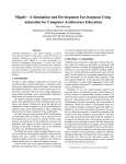
Design of an Experimental Unit for the Determination of
Oxygen Gas-Liquid Volumetric Mass Transfer Coefficients
using the Dynamic Re-oxygenation Method
ENE806
Laboratory Feasibility Studies in Environmental Engineering
Spring Semester 2007
Submitted to Dr. Syed A. Hashsham
Department of Civil and Environmental Enginneering
A126 Research Complex Engineering
Michigan State University
East Lansing, MI 48824
Dieter Tourlousse
&
Farhan Ahmad
1
Table of Contents
1. Summary
3
2. Introduction
4
3. Experimental Unit
6
3.1 Reactor configuration
6
3.2 Real time data acquisition
10
4. Experimental procedures
12
4.1. Preparation dissolved oxygen sensors
12
4.1.1 Sensor preparation
12
4.1.2 Sensor warm-up
12
4.1.3 Sensor calibration
13
4.1.3.1 Zero dissolved oxygen calibration point
13
4.1.3.2 Saturated dissolved oxygen calibration point
13
4.2. Communication with LabVIEW and data collection
5. Experiments
13
15
5.1. Reactor operating conditions
15
5.2. Determination of the sensor lag constant ks
16
5.3. Determination of the volumetric mass transfer coefficient kLa
17
6. Results and discussion
19
6.1. Sensor lag constant and effect on kLa measurements
19
6.2. Volumetric mass transfer coefficient kLa
21
7. Outlook
25
8. References
26
9. Appendix
27
2
1.
Summary
We report on the design and fabrication of an experimental laboratory unit for the
determination of the oxygen gas-liquid volumetric mass transfer coefficient kLa in a
bubble column reactor. The total cost of the unit was around $2,000 and required little or
no in-house modification of commercially available items. The reactor was hexagonal in
shape and had a column height-to-diameter ratio of 4. Three polarographic sensors were
implemented to measure dissolved oxygen concentrations at various axial positions in the
water column during oxygen absorption. To illustrate the performance of the
experimental unit, the kLa was determined in distilled water at ambient pressure and
temperature. Alongside, factors important in the determination of kLa in bubble column
reactors are discussed and evaluated, with focus on the impact of sensor lag and
hydrodynamic conditions in the reactor. It was verified that the estimated kLa (~0.31 min1
) was much larger than the sensor lag constant ks (~0.16 s-1), thereby justifying the
elimimation of sensor dynamics in modeling of the re-oxygenation profiles. In addition, it
was observed that re-oxygenation profiles were independent of the axial position of the
sensors in the reactor, thus allowing implementation of the continuous stirred tank reactor
(CSTR) model to estimate kLa. In conclusion, we constructed an experimental laboratory
unit for the estimation of kLa using the dynamic re-oxygenation method using
polarographic dissolved oxygen sensors. We provided experimental evidence that the
CSTR model without sensor lag can be adopted to extract kLa values from the measured
re-oxygenation profiles.
3
2.
Introduction
Efficient oxygen supply is a principal requirement for all aerobic chemical and
biological processes. Aeration refers to the process of addition of oxygen to water by
utilization of the principles of mass transfer. In most aerated biological processes, the
oxygen transfer rate (OTR) is modeled to be directly proportional to the driving force
generated by the difference between the saturation (DO*) and actual dissolved oxygen
concentration (DO) in the liquid phase. The proportionality constant is defined as the
volumetric mass transfer coefficient KLa (expressed in reciprocal time units), yielding the
following well-known relationship describing oxygen gas-liquid mass transfer:
OTR =
d ( DO )
= K L a(DO * − DO )
dt
with DO* obtained by Henry’s law. The KLa is a lumped parameter incorporating the
overall resistance to mass transfer and the total specific surface area available for mass
transfer:
1
1
1
=
+
K L a k L a Hk G a
where kL and kG represent the liquid and gas phase mass transfer coefficient, respectively,
and H the dimensionless Henry constant. In most cases, the liquid phase resistance to
mass transfer is dominating and the volumetric mass transfer coefficient is approximated
by kLa. The KLa depends on numerous parameters, including liquid phase properties,
reactor geometry and operating conditions.
The volumetric mass transfer coefficient kLa is a critical parameter in the design of
reactors and aeration systems. During the last decades various techniques for the
determination of kLa have been developed (Poughon et al., 2003 and references therein).
These methods can be separated into chemical and physical methods (Deront et al.,
1998). Chemical absorption methods can be classified depending on the reaction rates
4
with the sulfite oxidation method being the most widely adopted approach. Physical
oxygen absorption methods (based on gassing-in, gassing-out or pressure step) can be
dynamic or steady state. In the dynamic gassing-in or re-oxygenation method dissolved
oxygen concentration is monitored in the liquid phase during oxygen absorption. Though
inherent limitations of the method are well recognized (Gourich et al., 2006), the dynamic
re-oxygenation method using dissolved oxygen sensors has been increasingly adopted in
current studies on oxygen gas-liquid mass transfer.
A number of factors can confound the measurement of kLa. First, sensor lag can lead to
inaccurate dissolved oxygen concentration measurements and inferred kLa estimates
when the characteristic time of the sensor response and re-oxygenation dynamics are of
comparable magnitude (Vandu et al., 2004; Gourich et al., 2006). Increased sensor lag
leads to reduced estimates of kLa when this is not considered during modeling of the reoxygenation dynamics. Second, the hydrodynamic conditions in the reactor and position
of the dissolved oxygen sensors are critical for kLa estimations when perfect mixing is
not present (Gourich et al., 2006). Models to extract kLa from re-oxygenation profiles
need to incorporate the hydrodynamics conditions in the reactor if perfect mixing is not
present, and spatial gradients exist. This is of particular importance in bubble column
reactors where complete mixing is often not obtained.
The goal of this project was to design and build an experimental unit for the measurement
of the oxygen gas-liquid volumetric mass transfer coefficient kLa. A bubble column type
reactor was selected, and kLa estimated using the dynamic re-oxygenation method.
Polarographic dissolved oxygen sensors were implemented to measure dissolved oxygen
concentrations at various axial positions in the water column during oxygen absorption.
A series of experiments was performed to test the performance of the experimental unit,
with focus on i) determination of the sensor lag constant, and ii) determination of kLa in
distilled water as a demonstration of the developed experimental set-up. In conjunction
with this set of experiments a number of assumptions inherent to the estimation of kLa
based on the continuous stirred tank reactor (CSTR) model without sensor lag were
evaluated.
5
3.
Experimental Unit
3.1. Reactor configuration
The following section provides an overview of the various components of the
experimental unit. All components were commercially available (Table 1), and required
little or no modification. Although fabrication of a watertight and user-friendly sensor
seal was deemed challenging, we were able to manufacture a straightforward seal using
components available in a local hardware store (Home Depot, East Lansing, MI).
Figure 1. Experimental apparatus. Left panel. Major components of the experimental unit: 1,
compressed air and nitrogen cylinders connected in parallel; 2, non-calibrated rotameter; 3,
bubble column reactor; 4, air diffuser; 5, dissolved oxygen sensors (Vernier, Beaverton, OR); 6,
interface (LabPro, Vernier); 7, personal computer equipped with LabView and LoggerPro (30day demonstration version). Right panel. Dimensions of the bubble column (water column heightto-diameter ratio 3.8) and axial positioning of the dissolved oxygen sensors.
Bubble column. The bubble column reactor used in this study was an acrylic hexagonally
shaped tower aquarium with a height of 1.27 m and a diameter of 31.8 cm. The tower
aquarium was purchased from www.plasticsonline.com at a cost of $699 excluding
shipping costs. Considering the cost of individual acrylic sheets, the option of purchasing
an aquarium to serve as bubble column was deemed preferable in comparison with in-
6
house fabrication. Three holes were carefully drilled in the reactor to accommodate the
sensor seal (discussed below). The reactor was filled with water from the top of the
reactor using a plastic tube, and emptied rapidly (less than 5 min) by removal of the
sensor closed to the bottom of the reactor.
Table 1. Overview and cost of the components of the experimental unit.
Items
Catalog Number
Company
Cost ($)
Acrylic tower aquarium
(50"×12.5")
Dissolved oxygen sensor
Vernier LabPro
Monitor
Central processing unit
Reducing coupling
(1/2")
Reducer bushing
(3/4"×1/2")
O-ring washer
(3/4")
Gas cylinder
(Air & Nitrogen-230 scf)
Gas regulator, nitrogen
(single stage)
Gas regulator, air
(single stage)
Rotameter
Air diffuser
(top fin® round airstone, 3")
Air pump
(Stellar S-30)
Chemical resistant tubing,
Tygon (2" and 5")
Glass beaker (600 mL)
Glass flask (500 mL)
Glass flask (1 L)
Magnetic stirrer
Stirrer bar
HT-2
The Billiard Warehouse Inc.
699
DO-BTA
LABPRO
------------D2466
Vernier Software and Technology
Vernier Software and Technology
Panasonic
Colfax
Home Depot
3×199
220
200
400
3×1
438-101
Home Depot
3×1
------
Home Depot
3×0.5
------
Linde gas LLC
AIRCO
2×5
per month
100
CGA-580
CGA-590
Scott
100
B-250-5
------
-----PetSmart
---2.99
OE1042
PetSmart
20.99
Saint-Gobain
30
KIMAX, USA
KIMAX, USA
KIMAX, USA
VMR Scientific
STIR BARS
Total
5
22.06
34.82
3×98.33
3.50
$2,752
R-3603
FB-2610
27060-500
27060-1000
M-2200
SBM5108OTH
Air diffuser. The air diffuser (7.6 cm diameter, Figure 2) used during our initial set of
experiments was purchased from a local pet store (PetSmart, East Lansing, MI).
7
However, it is suggested that for future experiments air diffusers specifically designed for
bioreactor aeration should be adopted to yield a better control of the bubble size
distribution. The plastic tubing providing air flow to the diffuser was placed in a plastic
pipe taped to the reactor wall. The air diffuser was placed under the dissolved oxygen
sensors away from the center of he reactor to ensure adequate water circulation in the
vicinity of the sensors (Figure 2).
Figure 2. Left panel. Air diffuser. Right panel. Positioning of the air diffuser with respect to the
dissolved oxygen sensor.
Dissolved oxygen sensors. Three dissolved oxygen sensors were purchased from Vernier
Software & Technology (Vernier, Beaverton, OR). The sensors were relatively
inexpensive ($199 per sensor), but it should be recognized that it is recommended by the
manufacturer to adopt the sensor for teaching purposes only. It was, however, observed
that the sensors performed very well in terms of measurement of changes in dissolved
oxygen concentrations, even without calibration. Since estimation of oxygen gas-liquid
mass transfer coefficients merely relies upon the rate of changes in dissolved oxygen
concentration the sensors were deemed appropriate for our purposes. Adopting the
sensors to accurately measure absolute dissolved oxygen concentrations might, however,
require additional careful calibration and testing of the sensors.
The Vernier dissolved oxygen sensor is a Clark-type polarographic electrode sensing the
dissolved oxygen concentrations in liquid samples. A platinum cathode and Ag/AgCl
reference anode in KCl electrolyte are separated from the surrounding sample solution
by a oxygen-permeable membrane. A fixed voltage is applied to the platinum electrode,
8
and oxygen reaching the cathode undergoes the following reduction reaction:
½ O2 + H2O + 2e-→ 2OHSimultaneously the following reaction occurs at the anode:
Ag + Cl- → AgCl +e-
As a result, an electric current flows is generated proportional to the dissolved oxygen
concentration in the sampled solution. This current is converted to a proportional voltage,
amplified, and recorded.
Figure 3. Schematic depictionof the polarographic dissolved oxygen sensor.
Important. Polarographic dissolved oxygen sensors continuously consume oxygen, and
sufficient water flow around the sensor membrane should be ensured to eliminate an
apparent drop in dissolved oxygen concentration.
The sensors were placed across the water column at various axial positions. It was
important to reduce potential end effects that might occur if the sensors were placed too
close to the bottom of the column where aeration occurs, or too close to the top of the
water column. The lower sensor was placed ~19 cm above the bottom of the reactor, and
the two other probes were placed ~45 cm apart yielding a distance of ~14 cm between the
upper sensor and the level of the water column (Figure 1).
9
Sensor seal. Design of a seal allowing to readily insert and remove the dissolved oxygen
sensors was a critical part of the reactor. We were able to construct a simple sensor seal
using items readily available in a hardware store. A detailed view of the seal is presented
below along with the dimensions of the various components.
Importants. The threads of the various components (reducing coupling and reducer
bushing) purchased from the local hardware store were tapered, and needed to be
modified to allow for a tight seal.
Figure 4. Sensor seal. Upper panel. Individual components of the sensor seal. From left to right:
reducer bushing (3/4"×1/2"), O-ring washer (3/4"), reducing coupling (1/2"), rubber
gronmmet (provided with dissolved oxygen sensors). Lower panel. Sensor inserted in seal.
3.2. Real time data acquisition
Data acquisition constitutes sampling of the real world to generate data that can
be manipulated by a computer. The components of data acquisition systems (DAS)
include sensors to convert the measurement parameter to an electrical signal acquired by
the data acquisition hardware. Acquired data is displayed, analyzed, and stored on a
personal computer, either using vendor-supplied software, or custom displays. Data
acquisition begins with the physical phenomenon or physical property of an object (under
investigation) to be measured. This physical property or phenomenon could be the
temperature or temperature change of a room, the intensity or intensity change of a light
10
source, the pressure inside a chamber, the force applied to an object etc. A transducer
converts this physical property into a corresponding electrical signal, such as voltage or
current. The ability of a data acquisition system to measure different phenomena depends
on the transducers to convert the physical phenomena into signals measurable by the data
acquisition hardware. DAQ hardware is what usually interfaces between the sensor and a
personal computer. It can be in the form of modules that can be connected to the
computer's ports (parallel, serial, USB, etc.) or cards connected to slots (PCI, ISA) in a
mother board. Driver Software that usually comes with the DAQ hardware or from other
vendors, allows the operating system to recognize the DAQ hardware and programs to
access the signals being read by the DAQ hardware.
In this experiment a data acquisition interface named LabPro (Vernier Software and
Technology) was used. A schematic depiction of the module is presented below (Figure
5). LabPro can be connected to the USB port or serial port of a personal computer. The
interface contains two digital and four analog channels for connection of the sensors.
LabPro is compatible with LabVIEW, a highly user friendly environment for acquiring,
analyzing, displaying, and storing data.
Figure 5. Set-up of LabPro interface for collection of sensor readings.
LabVIEW provides a graphical programming environment highly suitable for data
acquisition. LabVIEW programs are called virtual instruments, or VIs, because their
11
appearance and operation imitate physical instruments. LabVIEW VIs contain the
following main components: the front panel, block diagram, and icon/connector. The
front panel provides the user an interface for data inputs and outputs. The user operates
the front panel by using the computer’s keyboard and mouse. Behind the front panel is
the block diagram that is responsible for the actual data flow between the inputs and the
outputs.
4.
Experimental procedures
4.1. Preparation of the dissolved oxygen sensors
The protocol for the preparation, warm-up and calibration of the sensors is
discussed below, and the protocol describing both steps can also be found in user’s guide
provided by the manufacturer (a reprint is provided in the appendix).
4.1.1. Sensor preparation
1. Remove the blue protective cap from the tip of the probe. This protective cap can be
discarded once the probe is unpacked.
2. Unscrew the membrane cap from the tip of the probe.
3. Using a pipet, fill the membrane cap with 1 mL of DO electrode filling solution.
4. Carefully thread the membrane cap back on to the electrode.
5. Place the probe into a beaker filled with 100 mL of distilled water.
4.1.2. Sensor warm-up
1. Plug the dissolved oxygen probe into the computer interface and open the LoggerPro
or LabVIEW software. The program will automatically identify the dissolved oxygen
probe.
2. It is necessary to warm-up the dissolved oxygen probe for 10 minutes before taking
readings. To warm up, leave it in water connected with the software for 10 minutes. The
probe must stay connected at all times to keep it warmed up. If disconnected for a few
minutes, it will be necessary to warm up the probe again.
12
4.1.3. Sensor calibration
4.1.3.1. Zero dissolved oxygen calibration point
1. Choose ‘calibrate’ from the experimental menu and click on ‘calibrate now’ button.
2. Remove the probe from the water and place the tip of the probe into the sodium sulfite
calibration solution. (Important: No air bubbles can be trapped below the tip of the probe
or probe will sense an inaccurate dissolved oxygen level. If the voltage does not rapidly
decrease, tap the side of the bottle with the probe to dislodge any bubbles. The readings
should be in the 0.2 to 0.5 V range).
3. Type 0 (the known value in mg/L) in the edit box.
4. When the displayed voltage reading for reading 1 stabilizes (~1 min), click ‘keep’.
4.1.3.2. Saturated dissolved oxygen calibration point
1. Rinse the probe with distilled water and gently blot dry.
2. Unscrew the lid of the calibration bottle provided with the probe. Slide the lid and
the rubber grommet about 1/2" into the probe body.
3. Add water to the bottle to a depth of 1/4" and screw the bottle into the cap.
4. Type the correct saturated dissolved oxygen value in mg/L (a table with dissolved
oxygen saturation values at different temperatures and barometric pressures is provided
in the user guide).
5. When the displayed voltage reading for reading 2 stabilizes (reading should be above 2
V), click ‘keep’ and then ‘done’.
4.2. Communication with LabVIEW and data collection
Instrument drivers simplify instrument control and reduce test program
development time by eliminating the need to learn the programming protocol for each
instrument. An instrument driver is a set of software routines that control a programmable
instrument. Each routine corresponds to a programmatic operation such as configuring,
reading from, writing to, and triggering the instrument. Use an instrument driver for
instrument control when possible. National Instruments provides thousands of instrument
drivers for a wide variety of instruments. Use the NI Instrument Driver Finder to search
13
for and install instrument drivers without leaving the LabVIEW development
environment. Select ‘Help’ to find instrument drivers to launch the ‘Instrument Driver
Finder’. One can also visit the NI Instrument Driver Network at www.ni.com/idnet to
find a driver for an instrument. If a driver is not available for an instrument, you can use
the Instrument I/O Assistant Express VI to communicate with the instrument. Before
starting to work with LabVIEW download the VIs from www.ni.com and install it on the
computer.
The following section provides a step-by-step guide describing the LabVIEW start-up ,
real time data collection, and storage. Additional information can be found in the user’s
manuals present in the laboratory.
Step 1. Open LabView and Click to open the user friendly VI program specially designed
for measuring real time data.
Step 2. The below presented window (Figure 6) will be displayed which shows the
overall block diagram for acquiring data. We have modified the real time measurement
VI to acquire the data for all the three probes and saving the data to the specified folder.
Step 3. Wire the resulting signal to either the graph (for waveforms) or the numeric (for
scalar values).
Step 4. Configure the Write LabVIEW Measurement File Express VI by double-clicking
it and make sure to provide a correct path for the file name.
Step 5. Save the file.
14
Figure 6. Programmed LabVIEW VI for collection of dissolved oxygen sensor readings.
5.
Experiments
5.1. Reactor operating conditions
Reactor operating variables including type of air diffuser, gas flow rate and
superficial gas velocity influence the re-oxygenation dynamics and inferred kLa. Hence,
knowledge about the operating conditions is vital to accommodate the interpretation of
kLa. The liquid phase was in all experiments distilled water, and experiments were
performed at ambient temperatue and pressure. Table 2 lists a number of reactor
operating parameters used during this study as measured by visual inspection. Gas and
liquid hold-up were estimated according to the volume expansion method based on
measurement of the height of the water column in the presence (H) and absence (H0) of
air bubbles using the following equations:
ε gas =
H − H0
ε
= 1 − ε gas
H
and liquid
15
Superficial gas velocity was estimated by interrupting the gas flow to the reactor and
monitoring the time required for the gas bubbles to reach the air-water interface (around
3.5 s). Notwithstanding potential inaccuracies in the measured reactor operating
conditions, the provided estimates should be useful in the design of further experiments.
However, more advanced methods, such as a high speed camera with dedicated software
tools, may be required to measure the superficial gas velocity and bubble size distribution
more accurately.
Table 2. Estimated reactor operating conditions.
Parameter
Condition
Superficial gas velocity
~0.3 m/s
Gas hold-up
~0.009
Bubble diameter
~7.5 mm
5.2. Determination of the sensor lag constant
Sensor lag was determined by subjecting the sensors to a near instantaneous
alteration in dissolved oxygen concentration, and collecting sensor readings until a
constant measurement was observed (Vandu et al., 2004; Philichi and Stenstrom, 1989).
The sensor was first equilibrated in a conically shaped beaker (500 mL) continuously
sparged with N2 provided using a gas cylinder. The sensor was then rapidly transferred to
a beaker (1000 mL) continuously stirred using a stir bar and magnetic stirrer. The
dissolved oxygen concentration was maintained at saturation by continuous sparging of
air using an air pump. The sensor dynamics was obtained by monitoring the dissolved
oxygen concentration every 0.2 s for a period of 1 min.
Important. It should be ensured that no gas build-up exists under the membrane
of the sensor. This was achieved by placing the stirrer bar away from the center touching
the glass of the flask.
Sensor lag was assumed to follow a first-order dynamics (Philichi and Stenstrom, 1989;
16
Letzel et al., 1999; Vandu et al., 2004; Gourich et al., 2006) according to the following
equation:
dDOm
= k p (DOl − DOm )
dt
where DOm represents the measured dissolved oxygen concentration, DOl the actual
dissolved oxygen concentration, and sp the sensor lag constant. After integration and
linearization this equation yields:
 DOl − DOm 
 = − k p (t − t 0 )
ln
0 
DO
−
DO
l
m 

with DOm0 the initial sensor dissolved oxygen measurement. This equation allows to
obtain sp based on the measured sensor dynamics. The experiment was repeated four
times, re-oxygenation profiles from each experiment analyzed separately, and sp and
related parameters reported as the aremathic mean and standard deviation of the
independent determinations.
5.3. Determination of the volumetric mass transfer coefficient
The volumetric mass transfer coefficient kLa was determined using the dynamic
oxygen absorption method (Letzel et al., 1999). Dissolved oxygen in the water column
was first removed by N2 sparging until the concentration fell below 1% of the dissolved
oxygen concentration at saturation (estimated at 8.66 mg/L at 23 °C and a oxygen partial
pressure of 0.21 atm). This step was generally achieved in about 30 min. Oxygen was
then introduced in the reactor as compressed air using a diffuser, and the dissolved
oxygen concentration monitored during re-oxygenation of the water phase every second
until saturation was reached. Switching between nitrogen and air sparging was achieved
by opening and closing the main valve of the gas cylinders. The gas cylinder outlet
pressure was furthermore adjusted prior to the experiment to yield a constant gas flow as
observed using a non-calibrated rotameter (level 11 at the rotameter used during our
17
experiments). However, this approach did not yield information on the actual air flow,
and it is suggested to calibrate the rotameter in order to accurately measure the gas flow
rate.
Re-oxygenation profiles were modeled according to the CSTR model without sensor lag:
d ( DO)
= k L a (DO * − DO )
dt
where DO represents the actual dissolved oxygen concentration in the liquid phase, DO*
the dissolved oxygen concentration in equilibrium with the gas phase calculated
according to Henry’s law, and kLa the liquid-side volumetric mass transfer coefficient.
After integration and linearization this equation can be adopted to obtain kLa as follows:
 DO * − DO
ln
 DO * − DO 0


 = − k L a(t − t 0 )


The experiment was repeated three times, re-oxygenation profiles from each experiment
analyzed separately, and kLa reported as the aremathic mean and standard deviation of
the independent determinations.
18
6.
Results and discussion
The dynamic re-oxygenation method was adopted to assess the gas-liquid
volumetric mass transfer coefficient kLa using polarographic sensors to monitor dissolved
oxygen concentrations in the water column. The sensor lag dynamics was determined to
verify the assumption that sensor lag dynamics was not significant in comparison with reoxygenation dynamics. The kLa was then estimated for distilled water under ambient
pressure and temperature, and the assumption of perfect mixing in the reactor justified.
6.1. Sensor lag constant and effect on kLa measurements
Sensor lag was evaluated by subjecting the sensors to a near instantaneous
alteration in dissolved oxygen concentration, and modeling the sensor lag according to a
first-order dynamics. A rapid
sensor response was observed, and a steady-state
measurement was usually observed in less than 30 s (Fig. 7). Sensor lag constants were
estimated at 0.18, 0.16, and 0.24 s-1 for the different sensors, equivalent to a 95% sensor
response time of 16.4, 18.2, and 12.3 s (Table 3). These estimates are in good agreement
with Gourich et al. (2006) who determined a sensor lag constant of 0.14 s-1. Vandu and
Krishna (2004) observed a sensor lag constant in the order of 0.47 s-1. The determined
95% sensor response time was, however, roughly two times smaller than the response
time reported by the manufacturer of the probes.
Table 3. Parameters of sensor lag dynamics (n=4).
ks (s-1)
ts (s)
t95 (s)
1 (0.6)
0.18 ± 0.01
5.6 ± 0.2
16.4 ± 0.5
2 (2.0)
0.16 ± 0.00
6.1 ± 0.1
18.2 ± 0.4
3 (3.4)
0.24 ± 0.00
4.1 ± 0.0
12.3 ± 0.1
Sensor number
(axial position, z/d)
19
Figure 7. Typical sensor dynamics obtained after a near instantaneous alteration in dissolved oxygen concentration.
20
Sensor lag can drastically influence the accuracy of dissolved oxygen measurements and
inferred kLa if the characteristics mass transfer time tm (1/kLa) is similar to the probe
response time ts (1/ks). Philichi and Stenstrom (1989) estimated that the product of the
sensor lag constant kp should be 50 times smaller than kLa to limit errors in kLa estimates
to less than 1%. Considering that the slowest responsing sensor displayed a ks of 0.16, it
was estimated that kLa values higher than 0.19 min-1 could be accurately measured with
the sensors used in this project. As demonstrated below, the kLa observed under the
specified reactor operating conditions was higher than this limit, and justified the
assumption that sensor lag did not significantly influence kLa estimates in our
experimental set-up.
6.2. Volumetric mass transfer coefficient kLa
The volumetric mass transfer coefficient kLa was determined using the dynamic
re-oxygenation method. Re-oxygenation was initiated by sparging of compressed air
using an air diffuser, and complete re-oxygenation was usually observed in less than 20
min (Fig. 8). The linearized plot demonstrated that a mono-exponential process governed
the re-oxygenation dynamics, further substantiating the assumption that sensor lag did not
noticeably influence the monitoring of the reoxygenation dynamics. Interestingly,
overlapping re-oxygenation profiles were obtained for all three sensors at different axial
positions with coefficients of variations among the always less than 5% (not shown). The
kLa was estimated at 0.31 ± 0.01 min-1 expressed as the arhematic mean and standard
deviation of the three independent determinations for all probes (Table 4), translating into
a time of 9.79 min to achieve 95% re-oxygenation of the water column.
The CSTR model is the most widely applied method to estimate kLa. This model assumes
perfect mixing in both the gas and liquid phase, and constant oxygen concentration in the
gas phase. For bubble column reactors with high water column height-to-diameter ratios,
however, the axial dispersion (AD) model might be more appropriate to account for nonperfect mixing by incorporation of a dependence of the gas and liquid phase oxygen
concentration on the axial position in the column (Han et al., 2007). The latter authors
observed that the CSTR and AD model produced different kLa values, in particular at
21
positions with increasing distance from the bottom of the reactor expressed as the axial
position divided by the diameter of the water column (z/dc). In this study, no large
difference was observed for kLa estimates at different axial distances (Table 4). This was
attributed to the fact that sensor furthest from the bottom of the water column has an axial
position of 3.8, and Han et al. (2007) observed that for sensor position-to-column
diameter ratios below 3 to 4 the AD and CSTR model yield nearly identical kLa
estimates. This demonstrated that our assumption of ideal mixing was justified, and the
BC reactor essentially behaved as a CSTR.
Table 4. Volumetric mass transfer coefficients kLa (n=3).
Sensor number
kLa
(axial position, z/d)
(min-1)
1 (0.6)
0.30 ± 0.01
2 (2.0)
0.30 ± 0.00
3 (3.4)
0.32 ± 0.00
Mean
0.31 ± 0.01
The volumetric mass transfer coefficient kLa in bubble column reactors is dependent on
various interrelated parameters, including the gas hold-up εgas, the superficial gas velocity
Ugas, and the specific interfacial gas-liquid surface area a. The specific interfacial gasliquid surface area is related to gas hold-up εgas and the mean bubble diameter db
(Wongsuchoto et al., 2003):
a=
6ε gas
d b (1 − ε gas )
Assuming that the bubbles in reactor posses an uniform diameter of 7.5 mm and a gas
hold-up of 0.009 (Table 2), the specific gas-liquid surface area was estimated at 7.2 m-1.
This in turn yields an estimated liquid-side mass transfer coefficient kL of 7×10-4 m/s.
This estimation is in good agreement with the value of 4×10-4 m/s reported by
Painmanakul et al. (2005).
22
Figure 8. Typical re-oxygenation dynamics. The arrow indicates start of the re-oxygenation process by air diffusion.
23
The estimated liquid-side mass transfer coefficient in bubble column reactors may vary
with superficial gas velocity Ugas depending on the range of Ugas (Vandu and Krishna,
2004 and references therein). The experiments in this initial study were performed in the
so-called churn-turbulent flow regimes (Ugas ≈ 0.3 m/s > 0.08 m/s). Vandu and Krishna
(2004) previously observed that the volumetric mass transfer coefficient per unit volume
(kLa/εgas) was independent of Ugas for velocities higher than 0.08 m/s. The authors
reported a kLa/εgas of 0.48 s-1 for a bubble column reactor with a height-to-diameter ratio
in the order of 4. This in excellent agreement with the value of 0.57 s-1 observed in this
study.
24
7.
Outlook
An experimental unit for the determination of volumetric mass transfer coefficient
kLa was designed and fabricated. The developed method adopts dissolved oxygen sensors
for monitoring of dissolved oxygen concentration during re-oxygenation of the water
column according to the dynamic method. Results obtained from an initial set of
experiments demonstrated that sensor lag was sufficiently small and could be ignored
during estimation of kLa. In addition, the bubble column reactor behaved similar to a
CSTR and no difference in kLa estimates at various axial positions was observed.
The experimental unit can be adopted to study the effect of various operating conditions,
such as superficial gas velocity and bubble size on the volumetric mass transfer
coefficient. A number of relevant studies pertaining to the effect of various reactor
operating conditions are provided in the references. These and similar studies may serve
as the basis for the design of future experiments.
25
8.
References
Vandu et al. (2004) Volumetric mass transfer coefficient in a slurry bubble column
operating in the heterogeneous flow regime. Chem Eng Sci 59 (22-23): 54175423.
Han et al. (2007) Gas-liquid mass transfer in a high pressure bubble column reactor with
different sparger designs. Chem Eng Sci 62 (1-2): 131-139.
Gourich et al. (2006) Improvement of oxygen mass transfer estimation from oxygen
concentration measurements in bubble column reactors. Chem Eng Sci 61 (18):
6218-6222
Vandu and Krishna (2004) Volumetric mass transfer coefficients in slurry bubble
columns operating in the churn-turbulent flow regime. Chem Eng Process 43 (8):
987-995.
Philichi and Stenstrom (1989) Effect of dissolved oxygen probe lag on oxygen transfer
parameter estimation. J Water Pollut Control 61, S3.
Letzel et al. (1999) Gas holdup and mass transfer in bubble column reactors operated at
elevated pressure. Chem Eng Sci 54: 2237–2246
Painmanakul et al. (2005) Effect of surfactants on liquid-side mass transfer coefficients.
Chem Eng Sci 60 (22): 6480-6491.
Wongsuchoto et al. (2003) Bubble size distribution and gas–liquid mass transfer in airlift
contactors. Chem Eng Sci 92: 81–90.
Data Acquisition Basics Manual, National Instruments, January 1998 Edition.
Function and VI Reference Manual, National Instruments, January 1998 Edition.
26
9.
Appendix
The appendix contains the following documents:
-
Material safety data sheet for sodium sulfite solution
-
Material safety data sheet for potassium chloride solution
-
Vernier dissolved oxygen sensor user’s guide
-
Vernier LabPro user’s manual
-
Dissolved oxygen saturation levels as function of temperature and pressure
27