Download SR4000 Manual

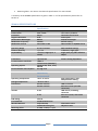
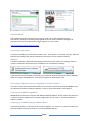
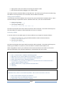
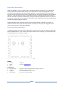
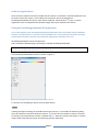
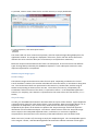
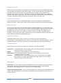
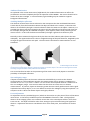
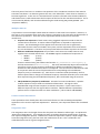
SR4000 User Manual
Version 0.1.2.2
Mesa Imaging AG
Technoparkstrasse 1
8005 Zurich
Switzerland
www.mesa-imaging.ch
Contents
1.
Intro ................................................................................................................................................. 3
Overview ............................................................................................................................................. 3
2.
Quick Start ....................................................................................................................................... 4
Package contents................................................................................................................................. 4
SR4000 Description and explanation of parts ..................................................................................... 5
SR4000 SPECIFICATIONS...................................................................................................................... 6
Installation and Setup.......................................................................................................................... 7
Installing Driver, Demo and Sample Software ................................................................................ 7
http://www.mesa-imaging.ch/drivers.php ..................................................................................... 8
Connecting a USB camera ............................................................................................................... 8
Connecting an Ethernet camera: using DHCP or static IP address ................................................. 8
Heat Sinking Requirements ........................................................................................................... 10
Power and Trigger Connections .................................................................................................... 10
Software Applications ....................................................................................................................... 11
Using the SwissRangerSampleGUI Application ................................................................................. 11
SR4000 output image types .......................................................................................................... 12
Important Adjustments ................................................................................................................ 13
What next? ........................................................................................................................................ 13
Visualizing and capturing 3D data using the SR_3D_View Application............................................. 15
3.
Using the SR4000........................................................................................................................... 18
How Time Of Flight Works................................................................................................................. 18
Signal Sampling and Saturation ..................................................................................................... 18
Measurement Accuracy ................................................................................................................ 19
Movement Artifacts ...................................................................................................................... 19
Getting your SR4000 to perform ....................................................................................................... 19
Physical setup ................................................................................................................................ 19
Camera Control Parameters .......................................................................................................... 21
Calculation of Cartesian Coordinates ............................................................................................ 23
Troubleshooting of camera positioning and adjustment .................................................................. 24
Ratings and Conformance ............................................................................................................. 25
API Intro............................................................................................................................................. 26
Documentation.................................................................................................................................. 26
Sample Code ...................................................................................................................................... 26
Matlab Interface ................................................................................................................................ 26
Page 2
1. Intro
Welcome to the SR4000 Manual. The SR4000 represents the fourth generation of Mesa Imaging’s
Time of Flight 3D cameras, and features significant advances in accuracy, stability and robustness.
This manual will be your guide to get the best performance from your SR4000.
Overview
The following section, ‘Quick Start’, gives a rapid introduction to the camera, its setup and use. At
the end of the section you will be capturing 3D images with the SR4000.
‘Using the SR4000’ delves into more detail of Time of Flight technology, and explains all the
capabilities and adjustments of the SR4000.
‘Detailed Specifications’ contains detailed technical specifications and ratings for the SR4000.
‘Software API Overview’ provides information on how to access the camera using the software API.
Page 3
2. Quick Start
Package contents
A standard SR4000 package contains:
1. SR4000 camera (USB or Ethernet)
2. Software and documentation Installation CD
Optionally, it may also contain the following items :
3.
4.
5.
6.
Communications cable (USB or Ethernet)
Power supply unit
Power cable
Trigger cable
Figure 1 SR4000 Package contents
Page 4
SR4000 Description and explanation of parts
The front view of the SR4000 is shown in Figure 2.
Illumination
cover
Optical Filter
Figure 2 Front view of SR4000
The following points are noted:


Optical Filter. This allows only light of wavelengths near that of the illumination LEDs to pass
into the camera lens.
Illumination LED cover. This protects the LEDs while allowing their light to be transmitted.
Cleaning the optics
Together the optical filter and the LED cover form a flat front face which may be cleaned by wiping
with a lint-free cloth, dampened with isopropyl alcohol if necessary, or with optical wipes. If the
front face is dirty with particles that may be abrasive, care must be taken not to scratch the surface.
Views of the SR4000 from the back and below are shown in Figure 3.
Status indicator LED
Power connector
Focus adjustment
Mounting holes
USB connector
Trigger connector
Figure 3 Back view showing connectors and view from below showing mounting holes
The following points are noted:





Power connector. For supply of 12V DC at up to 0.8A to the camera.
Trigger connector. For external hardware triggering of image acquisition.
Data Connector (USB in this case) For connection to PC.
Status LED. Flashing slow = power on. Flashing fast = acquiring images.
Focus adjustment. Do not alter this unless you have read Section 3 (Focus Adjustment).
Page 5

Mounting holes. See section ‘mechanical specifications’ for more details.
A summary of the SR4000 specifications is given in table 1. For full specifications please refer to
Section 3.
SR4000 SPECIFICATIONS
Performance
Specifications
Pixel Array Size
Field of View
Pixel Pitch
Angular Resolution
Illumination Wavelength
Modulation Frequency
Modulation Format
176 (h) x 144 (v)
43.6° x 34.6°
40 µm
0.23°
850nm
30 MHz
Sinusoidal or CBS
QCIF
Lens: F# 1.0, f=10mm
Horizontal and vertical
Center pixel
Central wavelength
Default setting
CBS available in 4Q2008 release
Operating Range
Distance Accuracy
Repeatability
0.3 to 5.0 meters
+/- 1 cm
< 5mm at range up to 2
meters
With standard settings
z-direction, single pixel
Single pixel (1σ); 50% reflective
object
Frame Rate
Communication Interfaces
Up to 54 FPS
USB 2.0
Fast Ethernet (100 Mb/s)
Windows XP, Vista, Linux,
MacOS
0.8 A @ 12 V
Camera setting dependent
Operating System
Electrical Power Consumption
Mechanical /
Environmental
Operating Temperature
+10 °C to +50 °C
Storage Temperature
Dimensions
-20 °C to +70 °C
65 x 65 x 68 mm
65 x 65 x 90 mm
IP Code
IP-54
IP-54
EMI Rating
Case Material
Window Material
Mounting Holes
Class A
Anodized Aluminum
Polycarbonate
Coated Borofloat glass
4 x M4; 2 x 4H7; 1 x 1/4”
Page 6
Case temperature, with
adequate heat sinking
USB 2.0 version
Ethernet version (includes
connector)
USB version, excluding
connector
Ethernet version, with rated
connector
Illumination cover
Objective cover
Installation and Setup
Driver software must be installed on the host PC before the camera will be recognised. It is
recommended to install the software first, and then plug in the camera. The installation procedure is
different depending on Operating System, and version. The different procedures are outlined below.
Also, any 3rd party Applications which use the camera may be installed at this stage.
Installing Driver, Demo and Sample Software
Suipported Operating systems are Windows XP, Windows Vista 32-bit, Linux and Max OS X.
Windows
The Setup program may run automatically when the CD is inserted. If not, run the Installer, e.g.
SwissrangerSetup1.0.10.550.exe from the root menu of the CD. Alternatively, run an updated
version of the Setup file downloaded from the Mesa website:
http://www.mesa-imaging.ch/drivers.php
On Windows Vista, some security confirmations must be ‘Allowed’ during the installation process.
The sequence for Windows Vista (32-bit) is as shown:
To enable support for Ethernet cameras, the Interfaces node must be expanded, and the Ethernet
checkbox checked.
Page 7
Linux and MacOS
The installation packages may be found on the CD under /Linux and /MacOS respectively.
Alternatively, please go to the Mesa Imaging Website for the latest installation packages and
instructions on how to install the Swissranger software on your system:
http://www.mesa-imaging.ch/drivers.php
Connecting a USB camera
The power and USB may be connected in either order. Once power is connected, the green Indicator
LED will start flashing slowly which indicates that the camera has successfully initialized.
Windows
A toolbar notification is displayed indicating that the Device Driver software is installing, and then
another indicates that the Device Driver installation has completed successfully.
If the device driver has installed successfully, any connected cameras will appear in Device Manager
under the category LibUSB Devices. Note that this applies to USB cameras only.
Connecting an Ethernet camera: using DHCP or static IP address
The order in which power and network cables are connected is important for Ethernet SR4000, since
this determines whether a fallback IP address is used, or the normal DHCP or static address.
Connecting to an SR4000 using DHCP
SR4000 Ethernet cameras are shipped with DHCP enabled by default. Simply connect the camera to
a network which has a DHCP server and then apply power to the camera. The camera obtains its
address via DHCP.
Connecting to an SR4000 using the fallback address
Instead of using DHCP, it is possible to set a static IP address. To connect to a camera in order to set
the static address it may be necessary to use a fixed fallback address:
Page 8
 Apply power to the unit without connecting the Ethernet cable.
 Wait 20 seconds before plugging in the network cable.
The camera now has a fixed IP address of 192.168.1.42. The camera cannot function normally using
this address: the only purpose is to set another static IP address as follows:
Setting a static IP address
It is necessary to set the IP address of the host PC first, (See notes below for Windows Vista.) Start a
Command Prompt or equivalent console. Windows Vista users, see note on Telnet below.
 Telnet to the camera
telnet 192.168.1.42
 set the static address, e.g.
fw_setenv staticip 192.168.1.33
Exit telnet and repower the camera with the network cable connected. The camera will always use
the static address on power-on when attached to a host pc or network.
Reverting to DHCP
To set the camera to use DHCP again, the static IP address must simply be cleared as follows:
 Telnet to the camera (e.g. using the fallback address mode as described above)
telnet 192.168.1.42
 clear the static address
fw_setenv staticip
Exit telnet and repower the camera with the network cable connected. The camera will always use
DHCP to get an address on power-on, when attached to a network with a DHCP server.
When using DHCP or static IP, the addresses of the connected cameras are visible in the Camera
Selection Dialog Box of the software applications, as described in the next section.
Windows Vista: Setting a static IP address on the host PC





Start -> Control Panel -> Network and Sharing Center
Right Click on your Local PC Name (This Computer) -> Properties
Select Internet Protocol Version 4 (TCP/IPv4), Click Properties
Select radio button Use the following IP address
Set IP Address, (e.g. 192.168.1.xx where xx is any other than 42 to communicate with a
camera using the fallback address.)
 Click on Subnet mask, to apply default of 255.255.255.0
 Click OK
 Click Close
Windows Vista: Enabling Telnet
In Windows Vista, Telnet is not installed by default. Here are the instructions to do this:
 Start->Control Panel->Programs and Features
 On left side, select ‘Turn Windows features on or off’
 Check Telnet, wait until it has been installed
Page 9
Heat Sinking Requirements
When the SR4000 is in use, especially when it will be operating for long periods, it is important to
ensure that there is adequate heat sinking. The requirements for heat sinking depends on the
environment and application, but the essential requirement is that sufficient heat is drawn away
from the camera to ensure that the external temperature of the camera housing does not exceed 50
degrees C. Heat may be drawn away by mounting the camera to a larger thermal mass (provided
that the mounting is thermally conductive), by using forced airflow (especially if there is any form of
enclosure), or by using a heat sink with ‘fins’ if a static system is required. A static fin-type heatsink is
available from Mesa Imaging if required.
Longer Integration Times cause the LEDs to be on for longer periods, resulting in more heat. To
reduce the amount of heat generated, and power consumed, it may help to use Triggered mode
rather than Continuous (see Triggered Modes).
Power and Trigger Connections
If a hardware trigger system exists this may also be connected at this stage. All cameras include two
Lumberg M8 connectors. One connects the power supply and one for trigger in- and output signals.
The pin assignments are shown in Figure 4.
Figure 4 Camera connectors are shown including numbering of pins.
POWER
1
2
3
+12VDC
SHIELD
GND
0.8A@12V
Connect to protective earth
TRIGGER I/O
1
2
3
4
External Voltage
Trigger In
Trigger Out
External GND
5V / 10mA – defines the logic level of the trigger output pin 3.
5V / 15mA - Start acquisition
5V - Frame integration / ready to fetch
In reference to External Voltage
Page 10
Software Applications
Once the driver software has been installed and the camera is connected, a software application may
be used to access the camera. In this Quick-start section the use of the applications
SwissRangerSampleGUI and SR_3D_View will be explained. Alternatively a 3rd party or custom
application which is compatible with the Swissranger API may be used with the camera.
Using the SwissRangerSampleGUI Application
This section applies to the SwissRangerSampleGui application which is available only on Windows.
However, the information is relevant to Linux and Mac users, since it describes the types of image
produced by the camera and the most important adjustments available to the user.
SwissRangerSampleGui can be launched from
Start->Programs->MesaImaging->Swissranger->Sample SwissRangerSampleGui
A notification may appear at this stage advising of a new driver dll version available on the Mesa
website. This may be downloaded by clicking on the link.
The SwissRangerSampleGUI Interface is shown in Figure 5.
Figure 5 SwissRangerSampleGui interface prior to opening a camera.
To connect to a SwissRanger camera, click the Open button.
->Open
A Dialog will appear showing the available Swissranger cameras. For example the following dialog
lists one USB camera and three Ethernet cameras. In this case the first Ethernet camera is selected.
An already-connected Ethernet camera is marked with a *. Note that ‘Camera File Stream’ is used to
replay camera data files previously recorded using another application.
Page 11
To proceed, select a camera from this list and click Connect, or simply doubleclick.
To start acquisition, click the Acquire button.
->Acquire
The camera will now start continuous acquisition, with the acquired images being displayed in the
application window. The images are displayed in false color, with a color bar above them which
indicates the color scale from blue (zero or minimum) to red (fullscale or maximum).
Below the Acquire and Close buttons the frame rate is displayed. In the next section the different
types of image data produced by the SR4000 are explained. In the subsequent section the most
important adjustments are explained.
SR4000 output image types
Distance Image
The Distance Image contains distance values for each pixel. Depending on whether the ‘Coord
Transf’ checkbox is checked, this is either radial distance from the camera, or the distance along the Z
axis. The raw distance values are represented in the camera by a 16-bit value, with the range 00xFFFF corresponding to distances from 0 to 5m. The Z value (and X and Y), computed by the
Coordinate Tranform function of the driver, is expressed in meters. In the SampleGUI application
however, for simplicity, the Z distance is represented on the same scale as the raw distance, i.e. 0 –
0xFFFF;
Greyscale Image
In reality, for the S4000 the illumination decreases with the square of the distance. Signal Amplitude
is therefore much lower for more distant objects, (see the Section ‘How Time of Flight Works’ for an
explanation of Amplitude.) The ‘Convert Gray’ mode removes this effect by multiplying the
Amplitude by the square of the distance to produce the ‘Grayscale Image’ with similar apparent
illumination of near and distant objects. The value is scaled so that at 2.5m the ‘Grayscale Image’
value is equal to the unadjusted Amplitude value. Furthermore, a correction is applied to
compensate for the unevenness in the intensity of the LED illumination over the field of view.
When ‘Conv Gray’ mode is off, this image is simply the Amplitude signal. The raw Amplitude signal is
in the range 0 – 0x7FFF, with the Most Significant Bit reserved to indicate saturation of the signal.
Page 12
Scaling of False Color
Below the Frame Rate Textbox is a dropdown control which allows selection of image0 and image1,
corresponding to the Distance and Grayscale images. The two edit boxes below this dropdown can
be used to set the range of the false color used to display the images. The top edit box is the
minimum range value. Any value at or below the value entered is displayed dark blue. The lower
edit box is the maximum range value. Any value at or above the value entered is displayed dark red.
All values in between are displayed with the proportional value on the color scale.
Important Adjustments
From the Settings menu, select Settings (dll dialog). This causes a dialog to be displayed which
contains two sliders. These can be used to control Integration Time and the Confidence Threshold.
Integration Time
This is the most important camera control available in the demo application. The Integration Time
can be adjusted using a slider control in the Camera Settings Dialog Box. Adjusting this value controls
how long each sensor pixel collects light. For lowest noise measurements the Integration Time
should be adjusted so that all (or at least most) pixels collect as much light as possible without
saturating. On the other other hand if a high frame rate is more important then the Integration time
may be reduced to achieve the desired frame rate.
Amplitude Threshold
Amplitude by itself can be used as a measure of the quality of corresponding distance
measurements. It can be adjusted using a slider control in the Camera Settings Dialog Box. A more
sophisticated measure of quality is given by the Confidence Map, described in the next Section.
Acquisition options
Below the Edit boxes used for the image color scaling are a set of four Tick Boxes:
Coord Transf
As explained under ‘Distance Image’ above, this switches between radial distance
and distance along the optical axis (Z).
Median
This applies a 3 by 3 median filter to the distance data.
Auto Exposure This automatically adjusts the Integration Time depending on the maximum
amplitudes present in the image.
Conv Gray
As explained under ‘Grayscale Image’ above, this is on by default in the SR4000,
which produces a distance-adjusted grayscale image. When it is off, the signal
Amplitude image is produced instead.
What next?
Refinements. The next chapter explains the fundamentals of Time of Flight distance measurement,
and outlines many aspects of the performance of a Time of Flight camera. These should be
understood to achieve performance for any application of the technology.
Capture and exporting 3D data. The next section descibes the use of the SR_3D_View application to
visualise and capture 3D data. The data may be subsequently processed offline by some custom or
3rd party software.
Page 13
SW development. For real-time applications where the camera data must be processed ‘on the fly’,
custom software is required. Appendix I contains an overview of options and resources for software
development using the SwissRanger API. For information regarding companies which supply relevant
software tools and solutions please contact Mesa Imaging.
Reference material for SW development on Windows, Linux, MacOS and Matlab. is available in the
MESA Knowledge base. Many Mesa customers have used Swissranger cameras with other platform
such as .Net and Labview. The knowledge base may contain tips from other customers that will help
you use the cameras.
Help and Support
For aspects of the setup and operation of the camera, refer to the Troubleshooting Section.
Have a look at the Knowledge Base and FAQ on the MESA website www.mesa-imaging.ch
Finally, send a question to the Mesa support team – [email protected]
Uninstalling and Reinstalling the Driver Software:
Sometimes issues with the driver software can be solved by reinstalling the driver, or installing an
updated driver version. Before doing either, it is important to unplug the camera and uninstall the
driver software.
This is done as follows:
Windows, Start->Programs->MesaImaging->SwissRanger->Uninstall
The driver may then be reinstalled as described in ‘Installation and Setup’.
Page 14
Visualizing and capturing 3D data using the SR_3D_View Application
The SR_3D_View application is installed by default when installing the driver from the CD.
Alternatively it may be downloaded from the mesa Imaging website at
http://www.mesa-imaging.ch/demosoftware.php
This software depends on DirectX being installed on the host PC (version 9c minimum).
Figure 6 The SR_3D_View Interface showing Distance, Grayscale and Confidence images on the left hand side and 3D
projection in the main window.
To connect to a SwissRanger camera, click the Start button.
->Start
The Distance, Grayscale and Confidence images will appear as shown in Figure 6 The SR_3D_View
Interface showing Distance, Grayscale and Confidence images on the left hand side and 3D projection
in the main window. The images on the left are unadjusted raw pixel arrays, whereas the 3D
projection has been adjusted by the coordinate transformation function in the driver to compensate
for radial distortion in the optics, removing the ‘pin cushion’ effect.
The Integration Time should be adjusted to avoid saturation and achieve the desired balance
between low noise and high frame rate.
Radio buttons select either full 3D representation ‘Pyramidal’ or ‘Perspective’ which is an
orthographic projection of the image plane of the measured pixel distances.
The 3D representation may be oriented using the mouse drags or arrow keys. Zoom is controlled by
the mouse scroll wheel or Page Up/Page Down keys.
For a summary of the main controls press F1.
Page 15
Elements of the main window may be configured from a menu which is activated by a right click.
These are:
Solid/Wire Frame/Point List
Methods of display of the 3D measured points
Color/Amplitude
Color coded distance, or grayscale signal Amplitude
Cross Section
Draws a red line through a single row and column of the data. The
postion of the line may be selected by clicking on the Distance or
Grayscale image.
Background
Background color can be selected from the pallette.
Additional adjustments:
Color scaling for color coded distance is selected using left and right clicks on the vertical color bar on
the right hand side of the display.
Center of rotation is adjusted along the Z axis using the CTRL and the horizontal mouse drag. This is
useful to enable rotation around an object of interest instead of around the camera.
HOME button on the keyboard brings the 3D scene back to the default view.
CTRL F12 shows the camera parameters dialog box which allows adjustment of IntegrationTime and
Amplitude Threshold.
CTRL R performs a left-right flip of the displayed images. By default the images are flipped L-R so
that the system gives ‘mirror’ behavior when the camera is set up facing towards the user (like a
webcam). This does not affect the layout of exported data.
Confidence Map
In addition to the Distance and Grayscale images, a third image is displayed, referred to as the
‘Confidence Map’. The SR4000 driver uses a combination of Distance and Amplitude measurements
and their temporal variations to compute a measure of probability or ‘confidence’ that the distance
measurement for each pixel is correct. This is represented in the ‘Confidence Map’. The Confidence
Map can be used to select regions containing measurements of high quality, reject measurements of
low quality, or even to obtain a confidence measure for a measurement derived from a combination
of many pixels. The Confidence Map has a range of 0-0xFFFF, with greater values representing
higher confidence.
Capturing Image Sequences
The ‘Streaming’ section of the interface enables capture of a number of frames of data. To do this,
the number of frames to be captured should be entered in the ‘Number of Frames’ Text Box, and
then the capture is started with the Start Button. Progress of the capture is indicated with a green
progress bar. Once capture is complete the data may be saved by clicking on Export. The root of the
data file names is entered, and the location of the saved files. Again, progress of the file saving is
indicated with a green progress bar.
Normal operation is resumed by clicking on the main Start button at the top left of the window.
Page 16
The format of the output files is explained below.
SR_3D_View Exported Range Image File Format
The SR_3D_View application can export a data stream from a SwissRanger camera containing 3D
point coordinates and Amplitude data.
Each captured range image in the sequence is saved in a separate file, with the filenames being
numbered name_0001.dat, name_0002.dat etc.
Within each file, Z, X and Y coordinates are arranged as arrays of 144 rows of 176 tab delimited
floats. Coordinates are in meters. The coordinate system is Right Handed, with Z being the distance
along the optical axis from the front face of the camera, and from the camera’s viewpoint, X
increasing to the left and Y increasing upwards, with zero X and Y lying on the optical axis.
This is followed by 144 rows of 176 tab delimited ints for the amplitude image. Amplitude full-scale is
0x7FFF.
Each array is preceded by a description e.g.
'% Calibrated Distance' indicates the Z coordinate array.
'% Calibrated xVector' indicates the X coordinate array.
'% Calibrated yVector' indicates the Y coordinate array.
'% Amplitude' indicates the amplitude array.
‘% Confidence map’ indicates the Confidence Map array.
If a threshold on Amplitude has been applied, all XYZ coordinates and Amplitude will be zero where
the Amplitude is below the threshold for the corresponding pixel.
A custom application may be coded to load this data for processing of the 3D point cloud sequence.
Capturing single frames
A single frame may be captured and exported in STL or DXF format in the following way:
When the camera is streaming live data, the Start button at the top left becomes a Stop button.
Clicking on this will freeze the data for the most recent frame. This may then be exported by clicking
on the File menu, and selecting the desired format.
Page 17
3. Using the SR4000
[Using it – details – taking control of the camera to get the best performance]
How Time Of Flight Works
The distance measurement capability of the SR4000 is based on the Time of Flight (TOF) principle.
In Time of Flight systems, the time taken for light to travel from an active illumination source to the
objects in the field of view and back to the sensor is measured. Given the speed of light c, the
distance can be determined directly from this round trip time.
To achieve the time of flight measurement the SR4000 modulates its illumination LEDS, and the
CCD/CMOS imaging sensor measures the phase of the returned modulated signal at each pixel. The
distance at each pixel is determined as a fraction of the one full cycle of the modulated signal, where
the distance correponding to one full cycle is given by
𝐷=
𝑐
2𝑓
(1)
where c is the speed of light and f is the modulation frequency. For the SR4000’s default
modulation frequency of 30MHz, this distance is 5.00m. The analog electrical signals are converted
into digital values in an Analog to Digital conversion process, from which a 16-bit distance is
calculated. This is the ‘raw’ output of the camera, with the full-phase value of 0xFFFF corresponding
to a distance of 5.00m. A 16-bit digital Amplitude signal is also produced. In the SR4000 this distance
measurement is performed at each pixel in the sensor, resulting in a 176 by 144 pixel depth map.
Figure 7 Time of Flight sampling of returned modulated signal
In Figure 7, the reflected signal is sampled four times in each cycle, at ¼ period phase shifts, i.e. 90°
phase angle. Signal B is the mean of the total light incident on the sensor: background plus
modulated signal, and A is the Amplitude of just the modulate signal. The phase θ is calculated from
the four samples to produce the distance measurement. The amplitude A may be used as a measure
of quality of the distance measurement, or to generate a grayscale image.
Signal Sampling and Saturation
During the pixel phase sampling process, two types of ‘saturation’ may occur, one which is due to
excessive background light, and the other due to excessive returned signal:
Page 18
1. The background illumination level B is too great, so that the charge wells in the pixels are
completely full by the end of an integration. When this is detected in a pixel, the MSB of the
resulting 16-bit Amplitude value is set and the distance value is set to zero. The design of the
SR4000 imaging chip incorporates a feature which suppresses the background light signal
from the A-D conversion process, however it cannot prevent this charge well saturation
effect.
2. Amplitude A is too large for the A-D conversion process. This is detected and flagged in the
hardware by checking a saturation threshold. When the amplitude is above the level
threshold the MSB of the Amplitude value is set and the distance value is set to 0.
Measurement Accuracy
Repeatibility of distance measurements depends mainly on signal amplitude and background
illumination. Signal amplitude in turn depends on distance and object reflectivity. The standard
deviation of distance measurements is often improved using some form of temporal or spatial
averaging. The optimal repeatability is achieved when the integration time is set to give the greatest
Amplitude without reaching saturation. If objects must be measured which have greatly differing
reflectivity or distance it is possible to take two separate exposures with different Integration Times
to achieve optimal signal amplitude for each object. In optimal situations a standard deviation in
single pixel distance measurement of less than 5mm is achievable.
Absolute accuracy on the other hand is independent of distance, and reflectivity. The absolute
accuracy is achieved internally in the SR4000 through a combination of elemements including pixel
and electrionics architectures, an optical feedback loop, and temperature compensations. In normal
operation an absolute accuracy of <1cm is achievable.
Movement Artifacts
Each of the 4 phase measurement samples are taken as a separate exposure. This means that in
order to obtain a phase/distance measurement, four consecutive exposures must be performed. If
an object in the scene moves during these exposures, systematic errors may be introduced into the
measurements. When there is significant local variation in the returned signal, the resulting distance
errors are larger than when objects are of more constant reflectivity.
Getting your SR4000 to perform
[Explain setup and use without obscuring important points with too much detail]
Physical setup
Camera should be mounted securely free airflow for cooling, free from vibration, with care taken to
ensure the following conditions:
Environmental conditions: temperature
Temperature range should be 10-50°C during operation. The camera should be thermally connected
to a heat sink if it will be used at temperatures near the maximum of this range. Alternatively, air
flow past the camera should be arranged to facilitate cooling. Using longer integration times causes
the camera to generate more heat than when using short integration times. Heat generation may be
minimized by using triggered acquisition.
Page 19
Ambient Illumination
As explained in the section How Time of Flight Works, the ambient illumination can affect the
performance and even completely disrupt the operation of the SR4000. The camera should not be
used at all in direct sunlight. In some situations, light shielding may be needed to suppress
background illumination.
Avoiding Multiple reflections
The distance measurement scheme is based on the assumption that the modulated illumination
travels directly from the llumination LEDS to the object and back to the camera, so that the total
distance of travelled by the light is twice the distance from the camera to the object. However, it is
possible that objects may be arranged in the scene such that light takes a less direct path than this.
For example, the light may be reflected off object 1, then object 2, before finally returning to the
camera sensor. In this case the distance travelled by the light is greater than the direct path.
Normally in these situation the light travels by the direct and also indirect paths (hence the term
multipath). The apparent distance is then a weighted average of the path distances, weighted by the
strength of signal returned via each path. The end result is that distance measurements are misestimated.
Figure 8 Positioning the camera to avoid reflections. The camera on the left may receive reflected light from the table
on which it is mounted, either directly as shown or indirectly via another object. The camera on the right has a better
mounting arrangement which avoids problems with reflection.
Care must therefore be taken in the positioning of the camera and nearby objects to avoid the
possibility of multipath reflections.
Non-ambiguity range
If objects could be present in the scene at distances which differ by more than the distance
corresponding to a full modulation period D, the measurement of their position is ambiguous: it
could be at x or at x + D, or even x + 2D etc. For this reason the full phase distance is referred to as
the ‘non-ambiguity range’. Care must be taken that this does not cause errors in distance
measurements. In practice, objects at distances greater than 5m usually produce much lower signal
amplitude than nearby objects, so it is not difficult to resolve the ambiguity using the amplitude. An
exception to this is when the distant objects are highly reflective.
Focus Adjustment
An adjustment screw is provided (Figure 1) which can be used to vary the point of focus of the 10mm
internal lens. In the factory calibration process the SR4000 is focused to 1.6m. The hyperfocal
distance of the imaging system is 2.5m which means that in this case objects will be in focus from
1.0m to 4.4m. The depth of field for other focus settings may be calculated using the hyperfocal
distance. Adjustment direction is anticlockwise for a closer focal point, and clockwise for further
away.
Page 20
The Focal point of the lens is a variable in the equations of the coordinate transform from radial to
Cartesian coordinates. At distances greater than 1m, it has little effect. Closer than 1m however, it
becomes significant. In this case it is assumed that the camera is focused at the measured distance,
and this distance is used to determine the focal point of the lens for the coordinate transform. This is
not activated by default, and must be enabled using the mode setting AM_CLOSE_RANGE. (See
‘Acquisition Modes’).
Multiple cameras
It is possible to connect multiple USB or Ethernet cameras to the same host computer. However, in
this case or in any situation when more than camera is operating in the same area the illumination of
the cameras may interfere. There are various approaches which can be used to avoid this
interference:
 Sequence the exposures of each camera using triggered acquisition mode so that the
cameras do not interfere. A custom software application is required to sequence the
cameras. The disadvantages of this approach are that the frame rate is significantly
diminished for each camera included in the system, and the acquisitions from each camera
are not simultaneous. The latter may be important when movement is present in the scene.
 Different modulation frequencies may be used in each camera to enable them to work
together with minimal interference. The SR4000 supports modulations frequencies of
o 29MHz
(5.17m)
o 30MHz
(5.00m)
o 31MHz
(4.84m)
These are selected using the software API function SR_SetModulationFrequency(),
and the enumeration ModulationFrq. The driver automatically adjusts the Coordinate
Transform to give correct Cartesian coordinates for different modulation frequencies;
however the raw 16-bit distance value it not adjusted. The raw value must therefore be used
in conjunction with the correct full-phase distance corresponding to the modulation
frequency used, as calculated in (1). Note that in continuous mode (see below), the first
frame acquired after a change in modulation frequency should be discarded, since it will have
been acquired using the old modulation frequency, but transformed using the new one.

CBS (Coded Binary Sequence) modulation. Instead of sine wave modulation, a pseudorandom sequence may be used to modulate the illumination. The signal is then
demodulated using the same sequence to measure the phase. If each camera uses a
different sequence, then the signals will not interfere. CBS has different repeatability
performance in comparison with sine wave modulation. [This is TBD for CBS SR4000.]
Camera Control Parameters
These parameters have already been discussed with reference to the SwissRangerSampleGUI
Application in the section ‘Important Adjustments’. However, some important details are considered
here:
Integration Time
The integration time is the length of time that the pixels are allowed to collect light. As explained in
‘How Time of Flight Works’, four samples are taken to produce the phase measurement, requiring
four separate integration periods. Therefore the total time required to capture a depth image is four
times the Integration Time, plus four times the readout time of 4ms. This is reflected in the
achievable frame rate for a given integration time.
Page 21
Amplitude Threshold
For static scenes, the reflected signal amplitude can be used as a measure of the quality of
corresponding distance measurements. An Amplitude Threshold is implemented in hardware in the
camera, so it consumes no host CPU resources.
Acquisition Modes
A number of Acquisition mode settings are supported by the SR4000. Some of these are only
accessible via the software API, using the SetMode() function.
Denoise ANF: A hardware-implemented noise filter is implemented in the SR4000. This filter
combines amplitude and distance information in a 5 by 5 neighbourhood. It reduces noise while
preserving detail, with no computational cost to the host CPU.
Confidence Map: an option controlling whether the Confidence Map is generated. If the Confidence
Map is not used in an application, use this option to stop it being generated, saving host CPU
processing resources.
Short Range: As explained in ‘Focus Adjustment’, the coordinate transform uses the actual measured
distance to determine the focal point for the transformation. This assumes that the camera is
focused at the measured distance.
Triggered Modes
Two modes of image acquisition are supported: continuous and triggered. In addition, in triggered
mode the acquisition may be triggered by either a software or a hardware trigger.
The trigger modes are enumerated in the software as follows:
AM_HW_TRIGGER
AM_SW_TRIGGER
hardware trigger mode
software trigger mode
The trigger modes are used in combination with the Acquire command as follows:
‘Continuous’ Mode
When software trigger mode is disabled, the camera continuously captures images. While
integration occurs for one image, the previous image is similtaneously processed in the internal
FPGA. When an Acquire command is received by the driver, the most recent image whose processing
has been completed by the FPGA is transferred to the host computer. However, the transfer does
not start until the beginning of the integration of the second subsequent (N + 2) frame. In this way a
high frame rate is achieved, but there is a latency in the acquisition after completion of integration of
one frame plus the transfer time.
The hardware trigger output is in active state for the duration of the integration, and the falling
transition of the hardware trigger output indicates that the integration is complete.
Important Note: in ‘Continuous’ Mode, because of the 1-frame latency, any changes in mode,
integration time or modulation frequency setting do not affect the first acquired frame after the
setting change, since this frame would have been acquired before the setting change.
Page 22
‘Triggered’ Modes
When software trigger mode is enabled, the camera does not capture an image until a trigger is
received. The following two cases are possible:
‘Software Trigger Mode’
When hardware trigger mode is disabled, the camera waits for an Acquire command. When
the command is received the image capture commences. The hardware trigger output is in
active state for the duration of the integration, and the falling transition of the hardware
trigger output indicates that the integration is complete. Once acquisition is complete the
image is processed in the FPGA and then transferred to the host computer. On completion
of the transfer the command completes. The aquired image is then available.
‘Hardware Trigger Mode’
When hardware trigger mode is enabled, the camera waits for an external hardware trigger.
When the trigger signal is received the image acquisition commences. The hardware trigger
output is in active state for the duration of the integration, and the falling transition of the
hardware trigger output indicates that the integration is complete. The Acquire command is
then used to initiate transfer of the image to the host computer. When the command
completes, the image is available. Hardware-triggered image capture may be parallelized
subject to the following timing limitations:



A second hardware trigger signal will trigger a new acquisition if it is received after
the first image has completed integration. The hardware trigger output may be used
by an external system to detect when the integration is complete.
If an Acquire command is not received before the next image has completed
integration then the first image is lost.
If the previous image transfer has not completed before a second integration
completes, the second image is lost.
It should be noted that the hardware trigger output indicates the period of integration in all trigger
modes, and can be used to synchronize an external system with the SR4000.
Calculation of Cartesian Coordinates
The software driver provides a Coordinate Transform function which converts the raw 16-bit radial
distances to Cartesian coordinates expressed in meters. This transformation includes a correction
which compensates for the radial distortion of the optics. The coordinate system is ‘Right-Handed’,
with Z coordinate increasing along the optical axis away from the camera, Y coordinate increasing
vertically upwards and X coordinate increasing horizontally to the left, all from the point of view of
the camera (or someone standing behind it). The origin of the coordinate system is at the interection
of the front face of the camera with the optical axis.
Page 23
Troubleshooting of camera positioning and adjustment
If a camera is not performing with expected accuracy, it can be helpful to check through each of the
following factors to eliminate possible causes:
Saturation
Signal Amplitude or ambient light is too great. The MSB of the pixel’s Amplitude value is flagged as
‘saturated’. This can be avoided by reducing the Integration Time, increasing the distance or
changing the angle of faces of reflective objects, or in some cases by shielding the scene from
ambient light.
Multipath
Causes distances to be overestimated. (described in more detail in ‘Avoiding Multipath reflections’).
This can be avoided by repositioning the camera or by blocking the indirect path.
Scattering
Objects with weak returned signal may have incorrect distance measurements due to interference
from objects adjacent to them in the image which have a much greater signal. This is caused by a
small amount of the light from the bright object being scattered by the optics to surrounding pixels.
To avoid this effect the camera should be repositioned, or an amplitude threshold applied.
Depth measurements are too noisy
Integration not long enough or too much ambient light. Lowest noise results are achieved when
objects are near enough to have plenty of signal but without saturation.
For troubleshooting of hardware and software-related issues, see the Help and Support
Page 24
Appendix I Detailed Specifications
TBD on conclusion of Qualification tests
Ratings and Conformance
TBD on conclusion of Qualification tests
Page 25
Appendix II
Software API Overview
API Intro
The Swissranger API for the SR4000 allows control of the camera and access to the image data from
user-developed software applications.
The API is provided as a .dll library file in Windows and and a .so library file in Linux. C++ header files
are provided which give the API function declarations, although the API may also be accessed from
other languages or environments such as C# .Net, LabView, Delphi, or Matlab.
Documentation
The SR API is documented in detail in the Compiled Help File Swissranger.chm which is installed with
the driver during installation on Windows. For Linux and Mac users this is also available as html on
the Mesa drivers page, http://www.mesa-imaging.ch/customer/drivers.php
Sample Code
Example code is provided in C++ with a simple GUI for Windows in the SwissrangerSampleGUI
sample, and without GUI for Windows and Linux in the LibusbSRTester.cpp ‘console’ application.
Some changes may be needed for the code to compile on different development platforms. Project
files are included for Microsoft Visual Studio 2005, and Makefiles are included for Linux.
Matlab Interface
A Matlab interface to the Swissranger is provided for Windows. This is installed by default during
driver installation to C:\Program Files\MesaImaging\Swissranger\matlab\swissranger
To make the Swissranger interface available within Matlab, this path must be added to the end of the
Matlab serach path using the Matlab Set Path command. The section of the Help file ‘Matlab
Interface to Swissranger Cameras’ contains more information. For an overview of the Swissranger mfunctions use the command help swissranger within Matlab.
Page 26