1
Ontario’s Landscape Tool
User’s Manual
Version 2013
Elkie P.C., A. Smiegielski* Julie Elliot, Rob Kushneriuk** and R.S. Rempel**. 2013.
Ontario’s Landscape Tool User’s Manual. Version 2013. Ontario Ministry of
Natural Resources. Policy Division, Forests Branch, Policy Section, Guides Unit.
Sault Ste. Marie Ontario.
* Ontario Ministry of Natural Resources, Science and Information, Geomatics Service Centre, Thunder Bay, Ontario.
** Ontario Ministry of Natural Resources, Applied Research and Development, Centre for Northern Forest
Ecosystem Research, Thunder Bay, Ontario
i
Contents
Overview ......................................................................................................................................................... 1
Installation ...................................................................................................................................................... 2
Deer Winter Yards and Moose Enhanced Areas ................................................................................. 4
Welcome TAB ................................................................................................................................................ 5
Science and Information Menu Item ........................................................................................................... 6
Provincial SRNV Tab .................................................................................................................................... 7
Provincial SRNV Tab ----- Box and Whisker Diagram sub-TAB ........................................................ 7
Box and Whisker Data sub-TAB .............................................................................................................. 9
Pattern Chart sub-TAB............................................................................................................................ 10
Pattern Data sub-TAB ........................................................................................................................... 11
Key Map sub-TAB ................................................................................................................................... 12
Tool Options Tab ......................................................................................................................................... 13
Scenarios Tab .............................................................................................................................................. 14
Create Scenario Button .......................................................................................................................... 14
Import/Export Scenario ........................................................................................................................... 21
Map Tab ........................................................................................................................................................ 18
Calculate Indicators Tab ............................................................................................................................. 21
Moose Emphasis Area Statistics .............................................................................................................. 24
Regional Forest Unit Moose Emphasis Area Classifications ........................................................... 25
Appendices ................................................................................................................................................... 27
Field Definitions – Appendix I ................................................................................................................ 27
LSL Procedures – Appendix II ................................................................................................................ 31
Prescriptive Indicators......................................................................................................................... 33
Evaluative Indicators ........................................................................................................................... 40
Forest Attribute look-up tables – Appendix III ...................................................................................... 84
Legends – Appendix IV .......................................................................................................................... 85
Age – Northwest, Northeast and GLSL Regions ............................................................................ 86
Barred Owl – GLSL - Region ............................................................................................................. 86
Beaver – GLSL .................................................................................................................................... 86
Black Bear - GLSL Region ................................................................................................................. 87
3
Black Bear Denning H.S.I. - GLSL Region ...................................................................................... 87
Black Bear Fall H.S.I. - GLSL Region .............................................................................................. 87
Black Bear Spring H.S.I. - GLSL Region ......................................................................................... 88
Black Bear Summer H.S.I. - GLSL Region...................................................................................... 88
Caribou Capability - Northwest Region ............................................................................................ 88
Caribou Refuge – Northwest Region................................................................................................ 89
Caribou Refuge 500 ha- Northwest Region .................................................................................... 89
Caribou Refuge 6,000 ha- Northwest Region ................................................................................. 89
Caribou Refuge 30,000 ha- Northwest Region ............................................................................... 90
Caribou Refuge Patches - Northwest Region ................................................................................. 90
Caribou Winter - Northwest Region .................................................................................................. 90
Caribou Winter 500 ha- Northwest Region...................................................................................... 91
Caribou Winter 6,000 ha- Northwest Region .................................................................................. 91
Caribou Winter 30,000 ha- Northwest Region ................................................................................ 91
Caribou Winter Patches - Northwest Region .................................................................................. 92
Conifer - Northwest Region ............................................................................................................... 92
Development Stage – Northwest, Northeast and GLSL Regions ................................................ 93
Ecosite – Northwest, Northeast and GLSL Regions ...................................................................... 93
Fisher - GLSL, Northwest and Northeast Region ........................................................................... 94
Forest Units - Northwest Region ....................................................................................................... 94
Forest Units - Northeast Region ....................................................................................................... 95
Forest Units - GLSL Region............................................................................................................... 95
Landscape Classes - Northwest Region.......................................................................................... 96
Landscape Classes - Northeast Region .......................................................................................... 96
Landscape Classes – GLSL - Region .............................................................................................. 97
Lynx - GLSL, Northwest and Northeast Region ............................................................................. 98
Management Type – GLSL, Northwest and Northeast Region.................................................... 98
Marten – GLSL..................................................................................................................................... 98
Marten NW - Northwest Region ........................................................................................................ 99
Marten NW 500ha - Northwest Region ............................................................................................ 99
Marten NW 3,000ha - Northwest Region ......................................................................................... 99
Marten NE - Northeast Region ........................................................................................................ 100
4
Marten NE Suitable 500 ha - Northeast Region ........................................................................... 100
Marten NE Suitable 5,000ha - Northeast Region ......................................................................... 100
Mature and Old Forest – Northwest and Northeast Region ....................................................... 101
Mature and Old Forest 50 ha – GLSL, Northwest and Northeast Region ................................ 101
Mature and Old Forest 500 ha – GLSL, Northwest and Northeast Region .............................. 101
Mature and Old Forest 5,000 ha– GLSL, Northwest and Northeast Region ........................... 102
Moose Bioclimatic – Northwest and Northeast Region ............................................................... 102
Moose Bioclimatic HSI – Northwest and Northeast Region ....................................................... 102
Moose Bioclimatic HSI Food – Northwest and Northeast Region ............................................. 103
Moose Bioclimatic HSI Food & Cover – Northwest and Northeast Region .............................. 103
Moose HSI Precipitation Coldest Quarter – Northwest and Northeast Region ....................... 103
Moose HSI Temperature Coldest Quarter – Northwest and Northeast Region ........................ 97
Moose HSI Temperature Warmest Quarter – Northwest and Northeast Region ...................... 97
Moose HSI Winter Cover – Northwest and Northeast Region ..................................................... 97
Moose – GLSL Region ....................................................................................................................... 98
Moose Aquatic Feeding k – GLSL .................................................................................................... 98
Moose Aquatic Habitat – GLSL, Northwest and Northeast Region ............................................. 98
Moose Dormant Season k – GLSL ................................................................................................... 99
Moose Growing Season k – GLSL ................................................................................................... 99
Moose Dormant Season Browse – GLSL, Northwest and Northeast Region............................ 99
Moose Dormant Season Range – GLSL, Northwest and Northeast Region ........................... 100
Moose Dormant Season Cover – GLSL, Northwest and Northeast Region ............................ 100
Moose Growing Season Forage – GLSL, Northwest and Northeast Region........................... 100
Moose Growing Season Range – GLSL, Northwest and Northeast Region ........................... 101
Moose Growing Season Cover – GLSL, Northwest and Northeast Region............................. 101
Northern Flying Squirrel – GLSL, Northwest and Northeast Region ......................................... 101
Northern Goshawk – GLSL .............................................................................................................. 102
Old Growth – GLSL, Northwest and Northeast Region ............................................................... 102
Pileated Woodpecker – GLSL ......................................................................................................... 102
Pine Warbler – GLSL ........................................................................................................................ 103
Red Shouldered Hawk – GLSL ....................................................................................................... 103
Red Squirrel – GLSL ......................................................................................................................... 103
5
Red and White Pine – GLSL ........................................................................................................... 104
Red and White Pine 50 ha – GLSL ................................................................................................ 104
Red and White Pine 500 ha – GLSL .............................................................................................. 104
Red and White Pine 5,000 ha – GLSL ........................................................................................... 105
Ruffed Grouse – GLSL ..................................................................................................................... 105
Snowshoe Hare – GLSL, Northwest and Northeast Region....................................................... 105
Southern Flying Squirrel – GLSL .................................................................................................... 106
Spruce Grouse – GLSL .................................................................................................................... 106
Summer Deer Carrying Capacity – GLSL ..................................................................................... 106
Summer Deer Carrying Capacity 500 ha – GLSL ........................................................................ 107
Summer Deer Carrying Capacity 60 km2 – GLSL ....................................................................... 107
Summer Deer Carrying Capacity 2000 km2 – GLSL .................................................................. 107
Summer Deer Forage All – GLSL ................................................................................................... 108
Summer Deer Forage Forest – GLSL ............................................................................................ 108
Summer Deer Forage Non-Forest – GLSL ................................................................................... 108
Summer Deer Forage Forest – GLSL ............................................................................................ 109
Wood Duck – GLSL .......................................................................................................................... 109
Young Forest – GLSL, Northwest and Northeast Region ........................................................... 110
Songbird models and legends – Appendix V .................................................................................... 111
Songbird legends – Northwest and Northeast Region ................................................................ 113
6
Overview
We designed Ontario’s Landscape Tool (OLT) considering the wide range of
stakeholders who may wish to access the science and information that was used in the
development of Ontario’s Landscape Guides. OLT provides a direct link to several
Science and Information Packages. These packages contain summaries of inputs,
rationale, simulation results and decision support tools that can be used when writing a
forest management plan or for testing model inputs, assumptions and results.
OLT contains routines which allow the user to import digital forest resource inventories
and perform analyses and comparisons consistent with the analyses and results which
were produced from the simulation. These routines provide the user with techniques to
compare existing or planned landscapes (i.e., forest harvest plans) with simulation
results including estimates of the simulated ranges of natural variation (SRNV).
Page 1
Installation
Double click on the “OltSetUpxxxx.exe” file to
begin the installation. The first screen will
indicate that the OLT installation is being
prepared and the necessary files are being
extracted.
You will be prompted to continue the install.
You must accept the Ontario Ministry of Natural
Resources Electronic Intellectual Property EndUser Licence Agreement before installation. This
licence is for all components of OLT and LSL. If
you do not accept this licence then you must
remove all components of OLT and LSL from
your computer.
This installation package does not prompt the
user for installation locations. OLT will be
installed in two spots. The program (olt.exe)
will into the systems Progam Files folder.
Working and data files will be installed into a
Programdata folder.
Next you will be prompted with a final screen
for installation.
Page 2
The OLT installation may take several minutes as
it copies various files to the location you chose.
Once the installation has completed click on
Finish.
The OLT icon will appear on your desktop, double
click on the icon to start OLT.
Landscape Scripting Language (LSL) is a spatial modeling system developed at the
Ontario Ministry of Natural Resource’s Centre for Northern Ecosystem Research
(CNFER) in Thunder Bay. It serves as the analytical engine within OLT and is used to
estimate indicator amounts and texture for specific areas. If you have already installed
LSL on your computer the OLT installation routines will not overwrite the current
version. The OLT installation will install a version of
LSL
that has been tested with a set of indicator scripts
appropriate for use with OLT. Depending on the
operating system that you are using a 64 or 32-bit
version of LSL will be installed. The version of LSL
is highlighted in the OLT title bar.
Once you have completed the install you will be able to run a basic version of OLT but
you will not be able to create scenarios or access the Science and information
Packages.
If you wish to view and access the Science and Information Packages from the OLT
menu, extract the science packages from the “Science and Information Packages”
archived zip file to the “C:\ProgramData\OltData\OLT\ScienceInfo” folder. You can
extract these word documents and use them in any folder; however if you wish to
access them through OLT they must be placed in this location.
If you wish to run Boreal indicator models extract all files from the “Boreal_NRVIS” zip
file to the “C:\ProgramData\OltData\OLT\NRVIS” folder. If these files are not placed
in this directory you will not be able to run Boreal models or create scenarios.
If you wish to run GLSL indicator models extract all files from the “GLSL_NRVIS” zip file
to the “C:\ProgramData\OltData\OLT\NRVIS” folder. If these files are not placed in this
directory you will not be able to run GLSL models or create scenarios.
Page 3
Deer Winter Yards and Moose Enhanced Areas
OLT will enable both a deer yards and moose enhanced area models providing a file
representing either exist in the NRVIS folder prior to creating a scenario.
The deer yards files must include the full suite of files associated
with a shape file. The DBF file should include a YARD_ID field.
This numeric field should contain a unique label for each unique
deer yard. OLT will allow the user to select from this field to do
analysis.
Similar to deer winter yards, a moose emphasis
area suite of files associated the a shape file
must exist if the user wishes to perform analysis
on unique moose emphasis areas. The DBF file
should include a MEA_ID field. This numeric field
should contain a unique label for each unique
moose emphasis area
Page 4
Welcome TAB
When you first start OLT a welcome screen will open. At this level five tabs and one
menu item are available:
Tabs
i)
ii)
iii)
iv)
v)
vi)
Welcome (current display),
Provincial SRNV,
Scenarios,
Songbird Models,
Tool Options and
About.
Page 5
Science and Information Menu Item
The Science Information menu item provides access to the Science and Information
Packages. These packages contain inputs, rationale, simulation results and several
tools which can be used when writing a forest management plan in Ontario. They also
include summaries of information used in the development of the landscape guide.
These packages are Adobe PDF files and will not open if you do not have Adobe reader
installed on your computer. We have embedded many documents, spreadsheets,
shape files etc. in the science packages and you will need Adobe Reader. The science
packages are password protected and therefore open as read only.
If a science and information package is greyed (unavailable), this means it has not
been installed. Refer to installation section (above) and ensure that the science and
information packages have been copied to the proper folder.
Click on any of the packages and the corresponding PDF.
Page 6
Provincial SRNV Tab
There are five sub-TABS located on the Provincial SRNV page; i) Box and Whisker
Diagram, ii) Box and Whisker Data, iii) Pattern Chart, iv) Pattern Data and v) Key
Map.
Provincial SRNV Tab ----- Box and Whisker Diagram sub-TAB
The Provincial SRNV (simulated range of natural variation) screen provides you with
access to SRNV results from each landscape simulation used in the development of the
landscape guide. The Box and Whisker Diagram sub-Tab provides access to SRNV
box and whisker plots. The simulated range of natural variation has been calculated for
prescriptive indicators (i.e., landscape classes, forest unit by development stage, old
growth, young forest and mature conifer) and evaluative indicators (i.e., various wildlife
species). Refer to Science and Information Package “A” for a complete list of species.
The SRNV are presented as box and whisker
plots including the median, minimum, maximum,
lower and upper quartile (25 th to 75th percentile)
from multiple simulations. Different simulation
periods, measurement periods and models were
used in each of the Landscape Guide Regions.
Refer to Science and Information package “A” for
complete descriptions.
At the bottom of the Provincial SRNV screen is an Area Filter with five radio buttons. By
clicking on these you can display simulation results (box-and-whisker diagrams) by
Forests, Ecodistricts (ED), Landscape Guide Regions (LGR), Wildlife Management
Units and Caribou Ranges.
Page 7
Once you have selected an area you
can then select a specific area based on
your filtering selection. The Area pulldown box on the left will list each area
for which SRNV’s have been calculated.
Select the pull-down box, a list of areas
will then pop-up. Use the side scroll bar
to view the entire list. Select the area
which you wish to view a SRNV.
Once you have selected an area you can
then select an Indicator to view SRNV.
The Indicator pull- down box will list all the
indicators that a SRNV has been estimated.
For several indicators a third choice, “Type”, must be selected. For example, SRNV’s
for unique forest units have been estimated. If you choose Forest Units as an indicator
you also must select the specific forest unit from the Type pull-down box.
You can scroll through each of these and the SRNV for a selected area by indicator by
type will be displayed.
Page 8
Box and Whisker Data sub-TAB
Click on the Box and Whisker Data sub-Tab will open a screen which displays the
data values specific to the current SRNV box-and-whisker plot.
The data values include the upper range, lower range, upper quartile, lower quartile,
median and year 0. Year 0 represents the value of the indicator at the start of the
simulation. Refer to the SRNV box and whisker plot – Y axis label for the units of the
indicator.
The Source information box lists the models used to estimate the current SRNV. The
Source Model Import Date information box lists the date that the current SRNV was
loaded into OLT and the Status box lists information specific to the area-extent that the
SRNV has been estimated.
Page 9
Pattern Chart sub-TAB
The Patten Chart sub-tab will only become active when an indicator that has pattern
data associated with it has been selected. These indicators include; mature and old
forest, caribou habitats, mature and old conifer (only in Northwest Region), marten
habitat and young forest.
For indicators with more than one scale of analysis (i.e., caribou and marten), select the
Scale drop down box and choose the scale of interest. With some indicators the first
class of the histogram will be dominant occupying most of the chart area. If this is the
case, select the Remove First Class check box and the graph will redraw with the first
class removed.
Page 10
Pattern Data sub-TAB
The Pattern Data sub-tab contains the data table from the pattern chart.
Page 11
Key Map sub-TAB
The key map sub-tab
will display a key map
illustrating the location
where the selected
SRNV is located
including the total land
area and in some
cases the crown land
area.
Once you have successfully
created a scenario the
scenario name with a
corresponding check box will
become visible on the right
hand side of the Provincial
SRNV page. Check this box to
plot the values of the current
scenario for comparisons to
the selected SRNV.
Page 12
Tool Options Tab
The Tools Option tab
provides you with several
options to consider when
running OLT.
Exit LSL on script
completion
If this box is not checked,
LSL will remain open when
it has finished executing a
specific indicator script. You
should leave this box
unchecked if you wish to
modify scripts or error check
scripts.
About Tab
The About TAB includes the
OLT credits. If using the OLT
for science and information
only then use first citation. If
using OLT to analyze spatial
data sets then use both the
OLT and LSL citations.
Page 13
Scenarios Tab
The Scenarios TAB is
used for importing and
creating scenarios from
either FIM compliant (Forest
Information Manual) forest
resource inventories (FRI)
or generic pre- classified
inventories (i.e., Patchworks
spatial plans). As you
import and create scenarios
they will be listed and
include information specific
to each scenario.
Create Scenario Button
If you wish to analyze a landscape, calculate
indicators and compare the landscape to a
set of SRNV results you must create a
scenario and import a shape file. Each
scenario represents a single landscape and
multiple scenarios can be compared.
Page 14
Creating a scenario is easy, select
the CreateScenarioB button. Enter
a Name for the scenario. The
name must be unique. If a scenario
with the same name exists – the
name will turn red. Choose the
location of the forest from the Area
pull-down box. It is important to
select the correct area. OLT will
classify your inventory into forest
units, landscape classes,
development stages etc. specific to
the area you select. If you choose
the wrong region you will be unable
to make correct comparisons to the
appropriate region. Similarly, the
evaluative indicators are specific to
each region and if you select the
wrong region you may not be able
to run one or more models.
The Region text (i.e., NW, NE or
GLSL) will change based on the
area you select.
When OLT classifies your inventory it uses the year-of-origin field to determine the age
of forest. Therefore you can select a Year to use as the base year for the
classifications. For instance, if you select 2008, the age of each polygon will be equal to
the year-of-origin subtracted from 2008. OLT does not grow the forest.
Page 15
Next Select the shape file that you
want to import. OLT will
automatically project the inventory
into the lambert coordinate
system*. To do this OLT needs to
know the projection of the selected
inventory. Therefore OLT requires
that a “*.prj” file accompanies your
inventory files. Consult with your
geographic information systems
officer if you need more information
on the “*.prj” file. If a “*.prj” file
does not exist with your shape file,
you will get a warning and the
inventory file name will be display
in red. You will not be able to
continue. UTM, Lambert and
geographic projections are
supported.
*The following is text from a typical lambert projection file as created in OLT:
PROJCS["MNR_Lambert_Conformal_Conic",GEOGCS["GCS_North_American_1983",DATUM["D_North_A
merican_1983",SPHEROID["GRS_1980",6378137.0,298.257222101]],PRIMEM["Greenwich",0.0],UNIT["D
egree",0.0174532925199433]],PROJECTION["Lambert_Conformal_Conic"],PARAMETER["False_Easting",
930000.0],PARAMETER["False_Northing",6430000.0],PARAMETER["Central_Meridian",85.0],PARAMETER["Standard_Parallel_1",44.5],PARAMETER["Standard_Parallel_2",53.5],PARAMETER["
Latitude_Of_Origin",0.0],UNIT["Meter",1.0]]
Page 16
Next you need to specify the format of the shape file – either a FIM Compliant
Inventory or Generic Inventory.
A FIM Compliant Inventory is a shape file that includes the following fields: SPCOMP,
SC, STKG, YRORG, POLYID ECOSITE1, DEVSTAGE, WG, HT and POLYTYPE. In
contrast, a Generic Inventory is a pre-classified shape file that contains LGFU
(landscape guide forest unit), LGAGE (landscape guide age), POLYTYPE and POLYID
(unique polygon number).
A FIM Compliant Inventory is usually plan start inventory while a Generic Inventory
can be any inventory that you classified outside of OLT and wish to import to evaluate
landscape indicators. Refer to appendices for a definition of the fields.
Page 17
Finally, there are two optional file selections to make; i) GLSL deer yards and ii) Moose
Emphasis Areas. The deer yards option is only available in the GLSL Landscape
regions while the Moose Emphasis Areas is available in all regions. Both files can be
anywhere on your system. OLT will make a copy of the file in the appropriate scenarios
folder in a subfolder called OptionalData.
CAUTION: OLT will project both the deer and moose files to the Lambert
projection. It is important that they are accompanied by a projection file and that
both of these files overlay on the scenario inventory. If either of these files does
not overlay on the scenarios inventories you will receive errors when attempting
to preform moose or deer analyses.
The deer yards file must contain the following three fields;
Field name
Field Type
Values
Stratum
String
0, 1, 2
Yard_ID
Numeric
1 - 999
Label
String
Yard name
The moose emphasis areas (MEA) file must contain the following fields;
Field name
Field Type
Values
Mea_id
Numeric
1 - 999
Label
String
Yard name
Note: Example files are installed in the “C:\ProgramData\OltData\OLT\NRVIS” folder.
Page 18
Once you have specified a scenario name, typed in a description, selected an inventory
shape file with a valid projection file and selected either a generic import or FIM import
and if applicable selected optional deer yards and moose emphasis areas file – then the
Create button will become activated. Click “Create” to begin the import process.
The import and scenario creation routines usually take between 15 minutes to 30
minutes. During this time OLT will import the shape file (geometry and attributes),
classify the shape file into landscape guide forest units, development stages and
landscape classes. OLT will then trigger LSL to build appropriate parcel (hexagon) files.
Once the install is complete a LOG file is generated which contains information about
the inventory (i.e., number of polygons imported and classified, warnings errors etc.).
You can open this file when prompted immediately following the import routines or you
can access the LOG text file later. You may also access the import log using the
Import log tab once a scenario has been loaded.
Page 19
OLT creates a scenario folder with the scenario name that you entered. The log file is
called “importlog.txt” and can be located in this folder and the typical folder structure
is: “C:\ProgramData\OLT\OLTData\Scenarios\Scenarioname”.
The newly created scenario does not load automatically when the import has finished.
You must load the scenario by either double clicking on the scenario or using your
mouse -right button - to show the Open - Delete selections. The quickest way to open a
scenario is to double click on the scenario name.
If you delete a scenario all models and reports will be deleted including the entire
directory/folder structure associates with that scenario.
Once a scenario has been loaded the scenario name will occur in the upper right
OLT ribbon. The Region that was selected during import is displayed including the
Area and the FRI import year. Five new tabs become available in the main OLT
screen (Map, Calculate Indicators, Generate Reports, View Reports and Import
Log).
Page 20
Import/Export Scenario
The import/export scenario buttons will allow you to export a scenario into
an archived file for the purposes of moving the scenario to another computer.
When exporting a scenario you will be prompted for a file name.
You will then be able to move that scenario to another computer with OLT
installed and, using the Import scenario button, import the scenario. This
allows you to transport scenarios between computers without having to
recreate the scenario. Note: although these are zipped files - you MUST use
the import and export scenario routines – unzipping the scenario outside of
OLT will not work.
These routines only allow you to move the base scenarios between
computers. Models that have been executed prior to an export will not
be included in the export files.
Page 21
Map Tab
When selecting the Map tab OLT uses a third party geographic information
viewer to open and display the inventory. When you first click on the Map tab a
blank map will appear. Click on the pull-down box under the OLT – “Select
Field” pull down selection box to view the various legends. After initial import
they include Age, Development Stage, Forest Unit, Landscape Classes,
Stocking and Ecosite1. The LSL will become active after an model has been
run (“Calculate Indicators”) using LSL. Similarly, the Songbirds tab will
become active after the songbirds model has been run (“Calculate Indicators”
Boreal only).
The Warnings tab includes legends which will display polygons that have
tagged as warning when importing the inventory. Usually these are not critical
generally representing polygons that have values that do not conform to the
standard for that class.
As you calculate indicators (discussed below) the results will relate back to the
shape file that you are currently viewing and the available selections in the
LSL legend list box will expand accordingly.
Page 18
The legends representing the import classifications (i.e., Age, Development
Stage, Forest Unit and Landscape Class) are region specific (i.e., NE, NW or
GLSL). The various warning legends (i.e., Polytype Warning, Site Class
Warning and Forest Unit Warning) will display your scenario inventory file with all
polygons that are warning and/or error free in green and polygons with a warning
and/or error in red.
This feature allows you to quickly review the validity of the classifications and
decide if you need to clean and re-import the scenario inventory. The import LOG
file provides a complete list of polygons, identified by PolyID, that contain errors or
warnings.
Page 19
OLT includes basic geographic information system functionality including:
i)
ii)
iii)
iv)
v)
vi)
Zoom-In,
Zoom-Out,
Pan,
Zoom Extents,
Identify and
Refresh.
OLT includes options for viewing Polygon Outlines (check box on left), Labels
including label field selection box and a label size slider selection.
Page 20
Calculate Indicators Tab
OLT contains LSL scripts which estimate both prescriptive and evaluative
indicators as highlighted in both the GLSL and Boreal Landscape Guides. The
Calculate Indicators tab is the location where you direct OLT to run these
scripts through LSL.
Select either Prescriptive or Evaluative Indicators and a list of available
indicators will be listed. Simply check the indicators that you would like to run and
then click on the Submit x to LSL button.
If you click on the Select All Types button, all indicators, both prescriptive
and evaluative, will be selected.
NOTE: If you wish to run multiple scripts – ensure that the Exit LSL on script
completion located in the Tool Options tab is selected. If you do not have this selected
LSL will stop after each indicator and wait for the user to close the LSL application.
Page 21
The Unselect All Types will clear all selections.
Use the Select All Models button on the right to select only prescriptive or
evaluative indicators. If you wish to run a single model, just click on that
indicator/model and ensure that no others are selected.
For a complete listing and definition of each model refer to Science Package “A”.
While running scripts LSL will
estimate the amount (usually area)
of each indicator. This is often
used to compare against the
SRNV.
PDF reports with texture maps and
histograms will be generated if
“Generate Reports” is selected.
Similarly, LSL will create hexagon
shape files and raster files if these
options are selected. This is
usually not required and the default
is No Output.
However, each shape file is
placed in the Shapefiles folder.
Page 22
Once submit your
request the bottom
status (OLT Queue and
OLT Job) will indicate
the approximate
position in the queue.
Page 23
Moose Emphasis Area Statistics
Ontario’s Forest Management Guide for Conserving Biodiversity at the Stand and
Site Scales include a set of standards, guidelines and best management practices
for moose emphasis areas.
When selecting either the “Moose” (Boreal regions) or “Moose GLSL” as the
evaluative indicator, moose emphasis area statistics will be calculated if a MEA is
selected.
Select the “Moose” (Boreal regions) or “Moose GLSL” as the evaluative indicator.
The Moose Parameters – Emphasis Area ID drop down box will become active.
Select the MEA ID of interest and submit the model. A “dbf” file will be created in
the “C:\ProgramData\OltData\Scenarios\ScenarioName\Evaluative\Moose GLSL”
folder (GLSL) or
“C:\ProgramData\OltData\Scenarios\Whitefeather\Evaluative\Moose” folder
(Boreal).
The guidelines provide direction on how to manage the productive forest within a
moose emphasis area as follows:
Within each LLP or area, manage the productive forest such that:
i. 5-30% of the forest is browse-producing habitat (generally stands <
35 years old and <10 m tall; or stands that have received a selection
cut within 10 years or a shelterwood regeneration cut within 20
years);
ii. 15-35% of the forest is mature conifer-dominated forest; and
iii. 20-55% of the forest is hardwood-dominated or mixedwood forest
≥35 years old or ≥10 m tall, or recent partial harvest areas that meet
the definition of residual forest.
A stand will only be attributed to one of the three criteria (e.g. a recent
partial harvest in a conifer stand may count towards criteria ii) or criteria
iii), but not both).
Page 24
If an optional moose emphasis area file was imported when a scenario was
created, browse producing, mature conifer and hardwood dominated and
mixedwood forest statistics will be calculated based on region specific forest units.
Regional Forest Unit Moose Emphasis Area Classifications
GLSL Conifer: CE1, HE1, LC1 PJ1, PJ2, PR1, PWOR, PWST, PWUS4,
PWUSC, PWUSH, SB1, SF1 , SP1.
GLSL Hardwood/Mixedwood: BW1, BY1, HDSL1, MWD, HDSL2, HDUS,
LWMW, MWR, MWUS, OAK, PO1.
Boreal East Conifer: PR1, PW1, PRW, SB1, PJ1, PJ2, LC1, SF1, SP1
Boreal West Conifer: PWDOM, PRDOM, PRWMX, OCLOW, PJDOM, SBMX1,
PJMX1, BFDOM.
Boreal East Hardwood/Mixedwood: LH1, TH1, PO1, BW1, MW1, MW2.
Boreal West Hardwood/Mixedwood: PODOM, BWDOM, OTHHD, HRDOM,
HRDMX.
Note: The mature conifer classification uses forest unit specific seral stage to
estimate mature and older.
The files include individual MEA statistics including:
Forest Area (TFOREST) in the MEA.
Browse area (BROWSE) in the MEA.
Proportion of browse (PBROWSE) in the MEA
Mature conifer area (MATCON) in the MEA
Proportion of mature conifer (PMATCON) in the MEA
Hardwood mixedwood area (HWDMIX) in the MEA
Proportion of hardwood and mixedwood (PHWDMIX) in the MEA.
Page 25
View Reports Tab
You can either open the PDF reports from the reports folder outside of OLT or
from within OLT - View Reports tab.
Double click on the
report of interest and
the report will open in
Adobe Reader.
Page 26
Appendices
Field Definitions – Appendix I
SPCOMP Field – species
S
composition
field.
P
C
Required
for FIM Compliant Import.
O
M
Field
type = String Field.
P
This field contains the species
F
composition
of each forested
ipolygon. The field lists the species
e order of relative dominance and
in
l
adds
up to 100(%). If a stand
d
composition does not add up to
100 a warning will be tagged to the
–
polygon.
Refer to Forest
Information Manual for a complete
sdescription.
p
e
cValid species values in SPCOMP
ifield. Species tagged with a “1” in
ethe UsedInQuery field are valid.
s
cValid species values in SPCOMP
ofield. This field contains the
m
species composition of a forested
ppolygon. The field lists the species
oin order of dominance and adds
sup to 100(%). If a stand
icomposition does not add up to
t100 a warning will be tagged to
ithe polygon. Refer to Forest
oInformation
n
Page 27
SC Field – site class field
Required for FIM Compliant
Import.
Field type =Numeric Field
The site class values range
from 0-4 and represent the site
productivity of a stand.
Refer to Forest Information
Manual for a complete
description.
STKG Field – stocking field
Required for FIM Compliant Import.
Field type =Numeric Field
The stocking field represents the stocking of the stand and usually contains
values from 0 to 1.0.
Valid values include 0.0, 0.1, 0.2, 0.3, 0.4, 0.5, 0.6, 0.7, 0.8, 0.9 and 1.0.
Refer to Forest Information Manual for a complete description.
YRORG Field – year of origin field
Required for FIM Compliant Import.
Field type =Numeric Field
This field typically contains the year the forest stand originated – often after a
stand replacing disturbance. Typical values include 1937, 1981, 2001 etc.
Refer to Forest Information Manual for a complete description.
Page 28
POLYID Field – polygon identification field
Required for FIM Compliant Import and Generic.
Field type = String Field
This field contains a unique numeric value for each polygon. Be careful with this
field. Although it contains numbers the format of the field is string and OLT does
not allow duplicate values.
POLYTYPE Field – polygon type field
Required for FIM Compliant Import and Generic Import
Field type = string
This field contains the land type within the polygon – see table for valid codes.
Note that only Polytype – “For” (productive forest) will be classified into a forest
unit.
DEVSTAGE Field – development stage type field
Required for FIM Compliant Import.
Refer to FIM technical specifications manual for typical values.
Field type = string
HT Field – height field
Required for FIM Compliant Import.
Refer to FIM technical specifications manual for typical values.
Field type = numeric
Ecosite1 Field – ecosite field
Required for FIM Compliant Import.
Refer to FIM technical specifications manual for typical values.
Field type = string
Page 29
LGFU Field – landscape guide forest unit field
Required for Generic Import.
Field type = string
Any generic string field that contains a forest unit classification can be used and
mapped to this LGFU field using the generic import function.
Valid forest unit codes are specific to each region (i.e., NE, NW and GLSL).
LGAGE Field – landscape guide age field
Required for Generic Import
Field type = numeric
This field represents the crown age of the forest stand.
Page 30
LSL Procedures – Appendix II
LSL uses hexagon parcel files when estimating landscape texture for each prescriptive
and evaluative indicator. These parcel files are created during the inventory import and
scenario creation. Parcel files contain the information associated with the intersection of
the inventory and a hexagonal grid.
A forest parcel file is created by intersecting the inventory with a 0.8 ha hexagonal grid
and this file is used in each of the prescriptive indicator scripts and two of the evaluative
indictor scripts (as noted below).
A habitat parcel is created by intersecting the inventory with a 1/7 ha hexagonal grid and
is used in all but two of the evaluative Indictor scripts. Additional parcels are created for
the Deer-Winter and Moose Emphasis Areas scripts by intersection the deer yards
and/or moose emphasis areas with a 1/7 ha hexagonal grid.
Other spatial layers are used in other evaluative indictor scripts and an LSL
hexagon grid which includes summaries of the data are built for each one. These layers
include:
•
a roads layer which contains the total length in metres of primary, secondary and
tertiary roads within each hexagon (1/7 ha scale)
•
a buildings layer containing the total number of buildings within each hexagon
(1/7 ha scale)
•
a streams layer containing the total length in metres of streams within each
hexagon (1/7 ha scale)
•
three climate layers which contain the area weighted mean for each
hexagon of the following climate data (0.8 ha scale):
•
temperature of the warmest three months of the year,
•
temperature of the coldest three months of the year,
•
precipitation of the coldest six months of the year.
For most prescriptive and evaluative scripts, initial assessment of forest structure and
habitat suitability uses the original LSL parcel file. The forest structure and habitat
suitability values are then summarized for each hexagon across the landscape.
Where hexagons intersect multiple polygons the area of forest classes are
Page 31
individually summed. For example, where a 0.8 ha hexagon intersects multiple
landscape classes, the area of each landscape class is calculated within each
hexagon. For habitat assessment where a mean suitability value is usually wanted,
an area weighted average is calculated for each hexagon.
Page 32
Prescriptive Indicators
Forest information is assessed at the 0.8 ha scale. Results are summarized and
illustrated within the reports at multiple scales as outlined below. The number of LSL
offsets used to average the results increases with increasing scale and is usually 4, 9 or
16 depending on the scale of the output.
For each prescriptive indicator the resulting proportions and forest patch areas of each
forest class or forest age group at each output scale, are summarized for every polygon
in the original inventory. This is done by assessing all forest dominated hexagons within
a polygon and calculating the mean proportion or majority patch area. The results are
then saved to a dbf file (FRI_Sscenario name) along with the corresponding Polygon ID
providing a link between the indicator and the starting inventory.
The resulting proportions and forest patch areas are also assigned to numbered bins
whose sizes are identical to those presented in the report charts and maps. The
resulting bin numbers are saved as binary raster files which can then be read into ESRI
to create grid files which illustrate the distribution of forest classes or a particular forest
age grouping across the inventory.
Page 33
Landscape Classes
Forest units and development stages are assessed and a landscape class is assigned
to each forest polygon section within each hexagon. The area of each landscape class
is then summed across the entire inventory and those values are saved to a dbf file
(P_Class_areas_scenario name). The area of each landscape class is then summed for
all 50, 500, 5,000 and 10,000 ha hexagons. These values are then averaged over
multiple offsets: 9 for the 50 and 500 ha scale and 16 for the 5,000 and 10,000 ha
scales. The proportion of each landscape class is then calculated for every hexagon at
each of the four scales, by dividing the total area of each landscape class by the total
forest area within the hexagon. These values are then averaged from the offsets. The
mean proportions of each landscape class at each scale are then averaged across the
entire inventory and those values are saved to a dbf file (P_Class_props_scenario
name). The scales are referenced within the dbf file with numbers: 2 for 50 ha, 3 for 500
ha, 4 for 5,000 ha, 5 for the 10,000 ha scale.
A regional analysis is then conducted at the 50 ha scale to locate forest patches of each
landscape class. At least 50 % of the hexagon forest area must be of a particular
landscape class for inclusion in a forest patch. The forest patch total areas of each
landscape class at each scale are then calculated.
Charts and corresponding maps are produced at the 0.8 ha scale illustrating the mean
proportion of each landscape class average over multiple 50 ha offsets. Charts and
maps at 50 ha, illustrating the distribution and sizes of forest patches of each of the
landscape classes, are included in the report.
The forest unit and development stage are also assessed and a forest unit-development
stage class (e.g. PJ1_P, ConMx_M, OAK_I) is assigned to each forest polygon section
within each hexagon. The area of each forest unit-development stage class is then
summed across the entire inventory and those values are saved to a dbf file
(FU_DS_scenario name).
Page 34
Young Forest
This script summarizes the forest into three young forest groups: Presapling forest (P),
Presapling-Sapling-Two-Staged (PST) and Young Forest (YF). The development stage
is assessed and forest that has a seral stage of either presapling, sapling or two-staged
is flagged for inclusion in the PST young forest group. Forest that has a seral stage of
presapling is flagged for inclusion in the P young forest group. The forest age is then
assessed and all forest with an age 35 years or younger is flagged as Young Forest
(YF). The area of each young forest group (P, PST and YF) is then summed across the
entire inventory and those values are saved to a dbf file (Young_scenario name). A
regional analysis is then conducted at the 15 ha scale to locate forest patches of each
young forest group. At least 50 % of the hexagon forest area must be of a particular
young forest group for inclusion in a forest patch. Reports are produced at the 15 ha
scale illustrating the distribution and sizes of forest patches of each of young forest
group.
Page 35
Mature and Old Forest
The development stage is assessed and forest that has a seral stage of mature, old or
two-staged is flagged as Mature+Old forest. The area of Mature+Old forest is then
summed across the entire inventory and that value is saved to a dbf file
(MO_F_scenario name). The area of Mature+Old forest is then summed for each
hexagon at 50, 500, and 5,000 hectares. The proportion of Mature+Old forest is then
calculated for every hexagon, at each of the three scales, by dividing the Mature+Old
forest area by the total forest area, within the hexagon. These values are then averaged
over multiple LSL offsets: 4 offsets for the 50 scale and 9 offsets for the 500 ha scale
and 16 offsets for the 5,000 ha scale. The mean proportion of Mature+Old forest at each
scale is then averaged across the entire inventory and those values are saved to the dbf
file mentioned above. Reports are produced at the 0.8 ha scale illustrating the mean
proportion of Mature+Old forest (average over multiple offsets) at each of the three
scales.
Page 36
Old Growth Forest
The forest unit and forest age are assessed within a look up table in order to flag areas
of forest considered to be Old Growth. Any forest with a seral stage of two-staged is not
considered as Old Growth forest since that forest area is included in the Mature+Old
forest area. The area of Old Growth forest is then summed across the entire inventory
and that value is saved to a dbf file (OG_scenario name). The area of Old Growth forest
for each forest unit is also summed across the entire inventory and those values are
saved to the same dbf file.
The area of Old Growth forest is then summed for each hexagon at 50, 500, 5,000,
20,000 and 50,000 hectares. The proportion of Old Growth forest is then calculated for
every hexagon, at each the five scales, by dividing the Old Growth forest area by the
total forest area, within the hexagon. These values are then averaged over multiple LSL
offsets: 9 for the 50, and 500 ha scales and 16 for the 5,000, 20,000 and 50,000
hectares. The mean proportion of Old growth forest at each scale is then averaged
across the entire inventory and those values are saved to the dbf file mentioned above.
Reports are produced at the 0.8 ha scale illustrating the mean proportion of each Old
Growth forest (average over multiple offsets) at each of the five scales.
Page 37
Conifer Forest (Boreal)
The forest unit is assessed within a look up table in order to flag areas of forest
considered to Conifer dominated. For inventories located in the Northwest Region these
areas include: PjDom, PjMx1, SbDom and SbMx1. For inventories located in the
Northeast Region, three Conifer forest groups are flagged. Areas with either a PJ1 or
PJ2 forest unit are classed as Jack Pine, areas with a SP1 or SF1 forest unit are
classed as Upland Spruce, and areas with a SB1 or LC1 forest unit are classed as
Lowland Spruce. For Northwest inventories, the area of conifer dominated forest is
summed across the entire inventory and that value saved to a dbf file (PC_F_scenario
name). For Northeast inventories, the areas of Jack Pine, Upland Spruce and Lowland
Spruce forest are summed across the entire inventory and those values are also saved
to a dbf file (filename is the same).
The areas of conifer dominated forest (NW) or Jack Pine, Upland Spruce and Lowland
Spruce forest (NE) are then summed for each hexagon at the 50, 500, and 5,000
hectares. The proportion of conifer forest is then calculated for every hexagon, at each
the three scales, by dividing the conifer forest area(s) by the total forest area, within the
hexagon. These values are then averaged over multiple LSL offsets: 4 offsets for the 50
scale and 9 offsets for the 500 ha scale and 16 offsets for the 5,000 ha scale. The mean
proportion of conifer dominated forest (NW) or Jack Pine, Upland Spruce and Lowland
Spruce forest (NE) at each scale is then averaged across the entire inventory and those
values are saved to a dbf file named above. Reports are produced at the 0.8 ha scale
illustrating the mean proportion of conifer forest (average over multiple offsets) at each
of the three scales.
Page 38
Pine Forest Units (GLSL)
The forest unit is assessed and any forest area classed as PWOR, PWUSC, PWUSH,
PWUS4 or PR is flagged as Pine forest. The area of pine forest is summed across the
entire inventory and that value saved to a dbf file (PRW_scenario name). The area of
pine forest is then summed for each hexagon at the 50, 500, and 5,000 ha scales. The
proportion of Pine forest is then calculated for every hexagon, at each the three scales,
by dividing the Pine forest area by the total forest area, within the hexagon. These
values are then averaged over multiple LSL offsets: 4 for the 50 scale and 9 for the 500
ha scale and 16 for the 5,000 ha scale. The mean proportion of Pine forest at each
scale is then averaged across the entire inventory and those values are saved to the dbf
file named above. Reports are produced at the 0.8 ha scale illustrating the mean
proportion of each Pine forest (average over multiple offsets) at each of the three
scales.
Page 39
Evaluative Indicators
Habitat suitability is assessed at the 1/7 ha scale for most wildlife species and 0.8 ha for
Boreal Songbirds and Boreal Bioclimatic Moose habitat. Results are summarized and
illustrated within the reports at the 1 ha scale and at broader scales for some of the
wildlife species (where noted below). Three offsets at the 1 ha scale are averaged to
produce the results seen within the charts. For larger scales, the number of offsets
increases with increasing scale and is usually 4, 9 or 16 depending on the scale of the
output.
For many of the evaluative Indicators, the forest unit and development stage is read in
from the inventory and assessed for habitat suitability using look up tables supplied by
the habitat model author. The total amount of forest, non-forest and water areas is
summed. Hexagons that are greater than 50 percent open water are eliminated from
the final habitat analysis.
In several evaluative indicator scripts a moving window analysis is conducted to sum
the area(s) of habitat component(s) within a specified radius. When this is carried out
the total area of each habitat component within the specified radius of a hexagon is
assigned to that hexagon. The resulting total area(s) will vary from hexagon to hexagon
depending upon a hexagon’s location relative to habitat areas across the landscape.
For several evaluative indicators reports are produced illustrating the distribution of
habitat across the inventory based on the percentage of used and preferred habitat
within each 1 ha. In these scripts the resulting percentages of used and preferred
habitat are assigned to one of five percentage bins: No habitat (NH), < 50% used
habitat (U), < 50% preferred habitat (P), >= 50% used habitat (DU) and >=50 %
preferred habitat (DP). The bins are also numbered 0 through 5 and the bin numbers
are saved as binary raster files which can then be read into ESRI to create grid files
which illustrate the distribution of used and preferred habitat across the inventory. For
the remaining evaluative indicators binary raster files are also created assigning the
final habitat suitability information to bins identical to those shown in the LSL reports.
Habitat suitability (HS) values within each evaluative indicator script are summarized for
each inventory polygon. This is done by calculating the mean HS value(s) of all
hexagons within each polygon. The results are then saved to a dbf file (FRI_Sscenario
Page 40
name) along with the corresponding Polygon id number. This will allow the user to link
the habitat suitability results back to their original inventory file. And where habitat
suitability values are grouped into percentage bins as described above, the majority
percentage grouping (NH, U, P, DU or DP) is determined for each polygon and also
saved the polygon linkable dbf file.
Note: Refer to Science and Information Package “A” for a non-LSL description of all
evaluative models.
Page 41
Barred Owl
The forest unit and development stage are each assessed for habitat suitability during
the breeding season and rated as used or preferred. The initial habitat suitability is the
minimum of the two suitability values.
A moving window analysis is conducted to sum the area of preferred nesting habitat
and the total area of used and preferred nesting habitat within a 150 ha home range
(700 m radius window). Hexagons with >= 40 ha of preferred nesting habitat are
assigned a habitat suitability value of 2 for nesting habitat. Remaining hexagons are
examined and hexagons with >= 40 ha of both used and preferred nesting habitat are
assigned a habitat suitability value of 1. All other hexagons are classed as non- habitat
and assigned a habitat suitability value of zero.
A regional analysis is then carried out to determine if there is any human disturbance
(roads, buildings and anthropogenic openings (forest unit GRS)) within 100 metres of
each hexagon. The habitat suitability of nesting areas is then reassessed and any
hexagon that is within the specified distance of human disturbance is no longer
classified as Barred Owl habitat.
The total area of Barred Owl nesting habitat is then summed for the entire inventory.
Reports are also produced illustrating the distribution of habitat across the inventory
based upon the percentage of used and/or preferred nesting habitat within each 1 ha of
area.
Page 42
Beaver
The forest unit is assessed to flag areas of open water. A regional analysis is then
conducted to determine the area of all water bodies in order to identify those that are
capable of supporting beavers. The area of each lake is assessed and lakes < 8 ha are
flagged as potential habitat. Large lakes (>= 8 ha) are only flagged only if they have
irregular shorelines (i.e. an irregularity value of >=3). This is determined by the following
calculation: Irregularity Value = Lake Perimeter / (2*((3.1415926 * Lake Area) ^ 0.5)).
Hexagons containing a stream segment are also flagged as potential habitat.
Hexagons that are located with 100 metres of a flagged water body and dominated by
non-water forest units are classified as preferred beaver foraging habitat. Hexagons
within 200 metres are classed as suitable beaver foraging habitat.
The forest unit and development stage are then assessed for food supply habitat
suitability and hexagons are rated either suitable or preferred based upon information
provided in lookup tables. Hexagons that are at least 50% BSH are also flagged as
suitable beaver foraging habitat.
The final beaver habitat classification (suitable or preferred) of each hexagon is the
minimum value of the foraging and food supply habitat components.
The total area of Beaver habitat is then summed for the entire inventory. Reports are
also produced illustrating the distribution of habitat across the inventory based upon the
percentage of used and/or preferred habitat within each 1 ha of area.
Page 43
Black-backed Woodpecker
The forest unit and development stage are each assessed for habitat suitability and
rated as used or preferred. The overall habitat suitability is the minimum of the two
suitability values. The total area of used and preferred Black-backed Woodpecker
habitat is then summed for the entire inventory. Reports are also produced illustrating
the distribution of habitat across the inventory based upon the percentage of used
and/or preferred habitat within each 1 ha of area.
Page 44
Black Bear
The forest unit and development stage of each hexagon are assessed for spring,
summer, fall, denning and cover habitat suitability. The habitat suitability classes are
either used or preferred for spring, summer, fall and denning habitat components and
just used for the cover habitat component.
The total habitat area for each of the first four habitat components (spring, summer,
denning and fall) is then summed for each hexagon as follows: area of preferred habitat
plus half of the used habitat area (i.e. Preferred + 0.5 * Used). For the cover habitat
component, the habitat area must be > 50% of the hexagon area to be assigned a cover
value of 1. All other hexagons are classed having no cover value and assigned a value
of zero.
This spring and summer habitat areas within each hexagon are then weighted
(adjusted downwards) depending on the hexagon’s distance from cover habitat, to a
maximum of 450 m. Spring or Summer habitat within 200 metres of cover habitat is
multiplied by a factor of one. Spring or summer habitat greater than 200 metres from
cover is multiplied by a factor that is less than one, which decreases with increasing
distance from cover habitat. Any hexagons with spring or summer habitat greater
than 450 m from cover habitat are classed as non-habitat.
A mean weighted habitat area for spring, summer and denning habitat components
within each hexagon is then calculated based on a moving window of 20 km2, the
estimated home range for black bears.
A moving window analysis is then done to sum the amount of fall bear habitat within a
65 km radius around each hexagon. The total area of surrounding fall habitat is then
converted to km2 and assessed in a lookup table to provide a multiplier value for
weighting the fall bear habitat suitability value of each hexagon. A hexagon retains a
value of 1 for fall habitat suitability if it has enough surrounding fall habitat to support a
density of 0.4 bears per km2. The fall habitat suitability value is weighted downwards
with decreasing amounts of surrounding fall habitat. Please refer to Science and
Information Package "B" for a more detailed description of this habitat analysis.
The overall suitability of each hexagon is then computed as a weighted arithmetic mean
of the four habitat suitability components, with the denning habitat suitability given ¼ the
Page 45
weight of the other seasonal suitability values: composite HSI = (Spring + Summer +
Fall + 0.25*Denning)/ 3.25
The weighted arithmetic mean, of each habitat component and overall suitability value,
for each 1/7 ha hexagon are then averaged at the 1 ha scale. Please note that these
mean values are based upon the mean habitat area at the 1/7 ha scale and it is those
value are illustrated within the LSL reports. Because the mean weighted habitat area is
based upon a 1/7 ha scale, the highest possible value for black bear habitat component
or overall habitat suitability would be 0.143. The resulting values for each habitat
component and the overall habitat suitability are also averaged for each inventory
polygon and saved to the polygon linkable dbf file.
Page 46
Boreal Songbirds
The Boreal Songbirds script is run using a 0.8 ha hexagonal grid. The forest unit and
forest age of each hexagon are then used to determine the following:
•
average age of the forest at 50 ha,
•
age edge density at 5000 ha,
•
percentage of hardwood (based on volume) at 50 ha,
•
mean stand crown closure at 50 ha,
•
mean stand height at 50 ha,
•
proportion of disturbance at 50 ha,
•
proportion of mature forest at 5000 ha.
The variables listed above are summed or averaged (as described below) at their
respective scale (50 or 5000 ha) with the resulting values averaged over multiple offsets
and assigned to a 50 ha hexagonal grid.
The age of the forest is averaged at the 50 ha scale by averaging the age of all 0.8 ha
hexagons within each 50 ha hexagon across the landscape. That value is then
averaged across 9 LSL offsets.
The age edge density is calculated by first assigning to each 0.8 ha hexagon an age
group value: 1 for mature and old forest, 2 for immature forest and 3 for presapling and
sapling forest. The length (m) of edge between forest stands is then weighted based on
the age group values of each adjoining stand. Where the difference in age group values
is 2 between the two adjoining stands, the length of edge is multiplied by a factor of 1.0.
Where the difference in age group values is 1, the length of edge is multiplied by a
factor of 0.5. The weighted edge length is then summed and averaged over 16 offsets
at the 5,000 ha scale.
The percentage of hardwood is calculated by using volumes curves to determine
individual tree species based up on the forest age and forest unit of each 0.8 ha
hexagon. The hardwood volumes within each 50 ha hexagon is then summed and
divided by the total tree volume. The percent of hardwood volume is then averaged over
9 offsets at the 50 ha scale.
Stand closure and stand height are determined for each 0.8 ha hexagon using Forest
Page 47
Attribute Look-up Tables developed by Phil Elkie, Arnold Rudy and Michael Gluck
(August 2004 – see Appendix). Each of these values are then averaged over 9 offsets
at the 50 ha scale.
Each 0.8 ha hexagon is classed as disturbed if the forest age is less than or equal to 20
and each hexagon is classed as mature if the forest age is greater than or equal to 80.
The area of disturbed forest is summed and divided by the total forest area at the 50 ha
scale. The area of mature forest is summed and divided by the total forest area at the
5000 ha scale. These values are then averaged over 9 offsets at the 50 ha scale. Once
all the forest variables have been calculated they are then used in equations developed
to determine the probability of songbird occupancy. Please refer to Science and
Information Package "B" for a description of these equations. The resulting probability
values are then averaged across the entire inventory. Reports are also produced
illustrating the distribution of the probability of songbird occupancy across the inventory
at the 1 ha scale.
The forest variables and the probability of songbird occupancy are averaged for each
inventory polygon and saved to the polygon linkable dbf file.
Page 48
Caribou
Winter Habitat (Conventional Boreal Model): The forest unit and forest age are
assessed for winter habitat suitability and classed as either used or preferred. The total
area of used and preferred caribou winter habitat is then summed for the entire
inventory. Reports are also produced illustrating the distribution of habitat across the
inventory based upon the percentage of used and preferred winter habitat within each
2
2
hexagon at the 1 ha, 500 ha and 60 km and 300 km scales.
Refuge Habitat (Conventional Boreal Model): The forest unit and forest age are
assessed for refuge habitat suitability. The total area of suitable refuge habitat is then
summed for the entire inventory. Reports are also produced illustrating the distribution
of habitat across the inventory based upon the percentage of suitable refuge habitat
within each hexagon at the 1 ha, 500 ha and 60 km2 and 300 km2 scales.
Capable Habitat (Conventional Boreal Model): The forest unit and forest age are
assessed for capable habitat suitability. The total area of capable habitat is then
summed for the entire inventory. Reports are also produced illustrating the distribution
of habitat across the inventory based upon the percentage of capable habitat within
each hexagon at the 1 ha scale.
Mature Conifer Habitat (Clay-belt Boreal Model): The forest unit and forest age are
assessed for habitat suitability. The total area of caribou mature conifer habitat is then
summed for the entire inventory. Reports are also produced illustrating the distribution
of habitat across the inventory based upon the percentage of caribou habitat within
each hexagon at the 1 ha, 500 ha and 60 km2 and 300 km2 scales.
Suitable Habitat (Clay-belt Boreal Model): The forest unit and forest age are assessed
for habitat suitability. The total area of suitable caribou habitat is then summed for the
entire inventory. Reports are also produced illustrating the distribution of habitat across
the inventory based upon the percentage of caribou habitat within each hexagon at the
1 ha, 500 ha and 60 km2 and 300 km2 scales.
Capable Habitat (Clay-belt Boreal Model): The forest unit and forest age are assessed
for habitat suitability. The total area of capable caribou habitat is then summed for the
entire inventory. Reports are also produced illustrating the distribution of habitat across
the inventory based upon the percentage of caribou habitat within each hexagon at the
Page 49
1 ha, 500 ha and 60 km2 and 300 km2 scales.
The mean proportions of all caribou habitat types are averaged for each inventory
polygon and saved to the polygon linkable dbf file.
Page 50
Deer – OWHAM adaptation - Summer Habitat
The forest unit and development stage are used to determine an estimate of the
biomass (kg/ha) of summer forage within each hexagon. For non-forested polygons
such as treed muskeg, only the forest unit is used to determine an estimate of summer
forage biomass. Hexagons that have a development stage of presapling or are classed
as brush and alder are flagged as security cover for deer. A regional analysis is then
conducted to located patches of cover. The summer forage value is then weighted
based upon the distance from a security cover patch. If the distance is 200 metres or
less than the forage value is multiplied by 1. Remaining forage values are multiplied by
the percentage of the hexagon that falls within 200 metres. Hexagons that are fully out
of the 200 metre range have their forage value reduced to zero. The deer carrying
capacity for each hexagon is then calculated by dividing the forage value by the
hexagon area (to determine the mean forage per hectare) and multiplying the result by
0.02: (Forage/0.14286) * 0.02.
The mean summer forage for all forested areas, all non forested areas and all land
areas is then calculated for the entire inventory. The mean summer forage within 200
metres of cover and the mean deer carrying capacity for the entire inventory is also
calculated. Reports are produced illustrating the deer summer carrying capacity at the 1
ha, 500 ha and 60 km2 and 2000 km2 scales. Reports are also produced illustrating the
distribution of summer forage of forested areas, non forest areas and areas within 200
metres of security cover, at the 1 ha, 500 ha and 60 km2 and 2000 km2 scales. All of the
deer summer forage available across the inventory is illustrated at the 1 ha scale only.
The deer carrying capacity values and the summer forage values for all forested areas,
all non-forested areas and all land areas, are averaged for every polygon, at each of the
four scales, and saved to the polygon linkable dbf file. All of the available summer
forage is averaged for every polygon at the 1 ha scale and also saved to the polygon
linkable dbf file.
Page 51
Deer – Winter Habitat
When running the Deer Winter script, the user will be able to select a Critical Thermal
Cover (CTC) threshold of the following values: 0, 10, 15, 20, 25 and 30%. This
threshold represents the percentage of critical thermal cover to maintain in order to
support an estimated deer yard carrying capacity. If the user selects a CTC value > 0,
the user will also have the option of having the LSL script select thermal cover patches
based upon ensuring a uniform distance between patches (spatial adjustment) as
determined by the CTC threshold. If the user selects a CTC value of 0%, all potential
deer winter habitat is reported and no Critical Thermal Cover threshold is applied nor is
any spatial readjustment carried out. The user will also be able to select a deer yard
stratum of the following values: 1, 1a, 2, 2a. A value of 1 or 1a will run analysis for
Stratum 1 only (deer yard core areas). A value of 2 or 2a will run analysis for Stratum 2
which is the entire deer yard. Selecting a value of 1a or 2a will turn on the spatial
adjustment part of the script. The CTC threshold value selected over rides the Stratum
value selected. If the user selects a 0% CTC threshold then no spatial readjustment is
carried out regardless of the Stratum value selected (i.e. 1 or 1a).
Note: If you wish to have a linkable FRI dbf output with only the area within a deer
yard file represented then you must ensure that the FRI that you create the
scenario has the deer yard boundary embedded.
The CTC threshold value and Stratum selected will determine what is included in the
LSL report and what fields are included within the output dbf files. Included below is a
list of what output is produced depending on CTC and Stratum values are selected. The
values selected will also determine the scale of some of the results presented in the
report and also the scale of the output shapefile(s). If no CTC threshold is set then all
results and the output shapefile will be at a 1 ha scale (the scale at which results for
most habitat models within the OLT are presented at). If the CTC threshold is greater
than 0 then charts and maps for Winter Cover Dominance (initial and adjusted) and
Critical Thermal Cover (before and after spatial adjustment) will be at the 50 ha scale.
All other charts and maps will be at a 1 ha scale. All output shapefiles (one for each LSL
offset) will be at the 50 ha scale. When the results are at 50 ha, it will be noted in the
chart X-axis titles and the map legend titles.
Page 52
The first step in assessing deer winter habitat is to use the species composition and
forest height to assign a cover quality ranking to each hexagon. There are 10 cover
rankings and they are grouped into three classifications: severe winter cover (cover
ranks 5 thru 10), moderate winter cover (cover ranks 2 thru 4) and access cover (cover
rank 1). The forest unit and development stage are then used to estimate browse
(kg/ha) within each hexagon.
The deer yard layer is read in; deer yards are located and their total forested area
calculated. A regional analysis is then conducted to locate forest patches of each cover
ranking value within each deer yard. If a CTC threshold greater than zero is selected,
the percentage of critical thermal cover is multiplied by the total deer yard forested area
to determine the area of forest to maintain for winter cover. Starting with forest patches
that have a cover ranking value of 10, the accumulative area of forest patches with a
cover ranking > 1 (i.e. moderate and severe winter cover only) is then compare to
amount of forest needed to retain in order to meet the CTC threshold. For example, if
the total area of cover rank 10 forest patches does not meet the CTC threshold area
then the area of cover rank 9 forest patches is added in. The area of lower ranking
forest patches is added in until the CTC threshold area has been reached. These forest
patches are then flagged to maintain for winter cover.
If the spatial adjustment part of the script is turned on (i.e. Stratum 1a or 2a is selected)
then the amount of forested area selected to maintain for deer winter cover is divided by
the number of 50 ha hexagons (with forest) within each deer yard. This provides an
estimate of the amount of forest to retain within each hexagon to distribute the winter
cover habitat across the deer yard as evenly as possible. Starting with forest that has a
cover ranking value of 10, the accumulative forest area with a cover ranking > 1 is then
compare to amount of forest to retain until the winter cover habitat area requirement is
met for each hexagon. After all hexagons are analyzed the total winter cover habitat that
has been selected is summed for the entire deer yard and compared with the desired
winter cover area to maintain. In some cases, the winter cover habitat area selected for
retention will be less than what is needed to reach the CTC threshold because some
hexagons may have less habitat area than needed habitat area for even distribution.
The shortfall is then made up by increasing the amount of forest selected in hexagons
Page 53
with a surplus of winter cover. This is carried out similar to the procedure described
above, but with the shortfall of winter cover area being divided by the number of
hexagons with surplus habitat to determine the amount of additional forest to retain
within each hexagon. A total of three passes across each deer yard are done to
spatially distribute the winter cover habitat as evenly as possible.
The browse values for each hexagon within each deer yard are summed and divided by
the yard area to provide an average browse (kg/ha). The average browse (kg/ha) is
then used to calculate a deer carrying capacity for each deer yard. The deer yard
carrying capacity is then used to calculate the total deer per yard. Please refer to
Science and Information Package "B" for a detailed description of these calculations.
Below is a list of what output is produced depending on CTC and Stratum values are
selected.
The Deer Winter LSL Report will include:
Note – reports can be accessed directly OLT-“View Reports” Tab or found in folder
– “programdata\oltdata\scenarios\scenarioname\reports”.
Deer Winter Carrying Capacity (Kw): The map and chart illustrate the deer winter
carrying capacity for the entire stratum selected.
Total Deer per Yard: The map and chart illustrate the total number of deer that can be
support for the entire stratum selected.
Browse Supply: The map and chart illustrate the kg per ha of browse summarized at
the 1 ha scale.
Quality of Deer Winter Cover: The map and chart illustrate the winter cover ranking of
the forest area at the 1 ha scale. All 10 rankings are presented as well as 0 value
representing forest that has no cover value. Grey areas represent areas with no forest
cover.
Proportion of Forest with Deer Winter Cover: The map and chart illustrate the
proportion of forest that has a cover ranking of 2 or greater.
Winter Cover Dominance:
All Available Habitat: The chart and map illustrate the cover habitat by group
rankings at the 1 ha scale. This output is very similar to the Quality of Deer Winter
Cover output except that the cover rankings are by Critical Thermal Cover value
Page 54
groupings: no cover value, cover value 1, cover values 2 to 4 and cover values 5 to
10.
Initial Selected Areas: The chart and map are produced only if the CTC threshold
selected is greater than 0. They illustrate the forest selected, by cover value
groupings, to meet at least the minimum area needed to reach the Critical Thermal
Cover threshold. The output is always at the 50 ha scale. The bin labeled “Cover
Not Selected” represents forest with a cover value of 2 or greater that is not selected
for retention to meet the CTC threshold. The results include all of the forest area of
the lowest cover value needed to reach the CTC forest area of the threshold
selected. Since all of the forest area of the lowest cover value is selected, the actual
percentage of forest selected may be greater than the CTC threshold.
It appears that areas with little or no cover value are now being selected and
assigned a higher cover value, but this is not the case. The chart and map illustrate
the dominant cover rank of the forest selected for retention within a 50 ha hexagon.
For example, if within a hexagon there are 40 ha of forest with a cover value of 1
and 10 ha of forest with a cover value of 8, the area would be shaded dark green to
show that the dominant cover value of the forest selected for retention is within the
Cover Value 5-10 Critical Thermal Cover grouping. Although the map illustrates
where and what type of forest needs to be retained for the CTC threshold it does not
illustrate the amount of forest needed. That information is presented in the dbf of the
LSL offset shapefile.
Adjusted Areas: The chart and map is produced only if the CTC threshold selected
is greater than 0 and the stratum value selected is either 1a or 2a. They illustrate the
forest selected by cover value groupings, to meet the area needed to reach the
Critical Thermal Cover threshold, spatially redistributed as evenly as possible with
only forested areas with cover values of 2 or great being selected. The percentage
of forest area selected for retention will be as close as possible to the CTC
threshold.
Once again, the map and chart map illustrate only where and what type of forest
needs to be retained and does not illustrate the amount of forest selected for
retention. That information is presented in the dbf of the LSL offset shapefile.
Critical Thermal Cover before spatial adjustment: The chart and map is produced
Page 55
only if the CTC threshold selected is greater than 0. They illustrate the proportion of
forest (with a cover value of 2 or greater) that is selected to meet at least the minimum
area needed to reach the Critical Thermal Cover threshold. The output is at the 50 ha
scale.
NOTE: The CTC charts and maps do not illustrate how much CTC habitat is within
each hexagon. The Critical Thermal Cover Supply chart and map illustrate the
proportion of forest that is needed within each hexagon to reach the CTC threshold.
Critical Thermal Cover after spatial adjustment: The chart and map is produced only
if the CTC threshold selected is greater than 0 and the stratum value selected is either
1a or 2a. They illustrate the proportion of forest (with a cover value of 2 or greater) that
is selected, after spatial adjustment, to meet the area needed to for CTC threshold. The
output is at a 50 ha scale.
The polygon linkable dbf file will include only the following fields if the CTC threshold
is set to 0:
Note: This file is named “\Scenarios\Scenarioname\Evaluative\deer
winter\CoreAreas\FRI_20.dbf”. Where FRI_##.dbf - ## refers to critical thermal
cover level.
PolyID:
Yard_ID:
Yard_Area:
Yard_ For:
PrPj:
Cov_rank:
Stratum:
the polygon ID number as listed in the inventory dbf file
a unique id number for the yard
area (ha) of the yard
the forested area (ha) within the yard
flags a stand that is pure red, white or jack pine
the cover rank value for a particular polygon within the deer yard
the stratum the polygon belongs to (1 = core areas, 2 = within deer yard, but
not part of the core area)
SW_area: the severe winter deer habitat area (ha) (cover ranks 5 thru 10) within the deer
yard
MW_area: the moderate winter deer habitat area (ha) (cover ranks 2 thru 4) within the
deer yard
AC_area: the access cover only winter deer habitat area (ha) (cover rank 1) within the
deer yard
T_browse: the total amount of browse – kg for the entire deer yard
Avgbrowse: the average kg/ha of browse
DCC:
Deer Carrying Capacity (deer per km2)
DPY:
Total Deer per Yard (based upon DCC)
Page 56
The polygon linkable dbf file will also include the following fields if the CTC threshold
is > 0:
Hab_Area: the deer habitat area (ha) within the yard needed to reach the (CTC) threshold
P_Hab:
the proportion of forest needed to reach the CTC threshold
CRU:
The cover ranks used to achieve the CTC threshold (a value of 3 means that
cover ranks 3 to 10 were needed to achieve the CTC threshold)
CTC_Flag1: Flags a stand that is selected to achieve the CTC threshold
The deer yard summary dbf file (e.g. S1_summary.dbf or S2_summary.dbf) is created
and if the CTC threshold is set to 0 and will include only the following fields:
Field
Description
Yard_ID
a unique id number for each deer yard
Yard_Area
area in hectares of the deer yard
T_Browse
the total amount of browse (kg)
AvgBrowse
the average kg/ha of browse
DCC
Deer Carrying Capacity (Ks) – deer per Km2
DPY
Total number of deer per yard (based upon DCC)
T_HabArea
the total area of winter cover habitat (cover ranks 1 to 10)
SW_area
the area of severe winter habitat (all polygons with cover ranks 5 to
10)
MW_area
the area of severe moderate winter habitat (all polygons with cover
ranks 2 to 4)
AC_area
the area of access cover habitat (all polygons with cover rank 1)
Yard_ For:
the forested area (ha) within the deer yard
p_CR1
the percentage of that total habitat area that is cover rank 1
p_CR2
the percentage of that total habitat area that is cover rank 2
p_CR3
the percentage of that total habitat area that is cover rank 3
p_CR4
the percentage of that total habitat area that is cover rank 4
p_CR5
the percentage of that total habitat area that is cover rank 5
p_CR6
the percentage of that total habitat area that is cover rank 6
p_CR7
the percentage of that total habitat area that is cover rank 7
p_CR8
the percentage of that total habitat area that is cover rank 8
p_CR9
the percentage of that total habitat area that is cover rank 9
p_CR10
the percentage of that total habitat area that is cover rank 10
The deer yard summary dbf file for a CTC threshold > 0 without spatial adjustment
(e.g. S2_CTCT20.dbf or S2_CTCT20_initial.dbf) will include all of the above fields as
well as the following additional fields:
Field
Description
CTCT_Area
the winter cover habitat area (ha) needed to reach the CTC
threshold
Hab_Area
the area (ha) of winter cover habitat of all cover ranks used to reach
the CTC threshold
P_Hab
the percentage of habitat area selected
Page 57
Status
the lowest cover rank class needed to reach the CTC threshold
CR_Used
the range of cover ranks used to reach the CTC threshold
The deer yard summary dbf file for a CTC threshold > 0 and with spatial adjustment
(e.g. S2_CTCT20_adjusted.dbf) will include the following fields:
Field
Description
Offset_ID
a unique id number for each LSL offset of each deer yard
Yard_ID
a unique id number for each deer yard
LSL_offset
a unique id number for each LSL offset
Yard_Area
area in hectares of the deer yard
For_ Area
the forested area (ha) within the deer yard
CTCT_Area
the winter cover habitat area needed to reach the CTC threshold
T_HabArea
the total area of winter cover habitat (cover ranks 1 thru 10)
Hab_Area
the area of winter cover habitat of all cover ranks used to reach the
CTC threshold
the initial percentage of habitat area selected
P_Hab
SW_area
the area of severe winter habitat selected
MW_area
the area of moderate winter habitat selected
A summary of stand cover ranking by deer yard will be created if the CTC threshold
is > 0 and will include the following fields (e.g. CA_data_.dbf):
Field
Description
SetID
a unique id number for each hexagon
Yard_ID
a unique id number for each deer yard
Yard_Area
area in hectares of the deer yard
Coverrank
the cover ranking value
For_Area
the forested area (ha) within the deer yard
Hab_forest
the cumulative forested area for all cover rank values from 10 to
that particular cover rank value (e.g. for a cover rank value of 5 this
field represents the forested area within the deer yard of all
polygons with cover rank values of 5 to 10
p_for_CR
the cumulative percentage of cover in the deer yard for all cover
rank values from 10 to that particular cover rank value
An LSL shapefile (e.g. S2_2_0_1.shp or S2-20_2_0_1.shp) will be created for all runs
and will include the following fields:
Field
Description
SetID
a unique id number for each hexagon
a unique id number for each deer yard
Yard_ID
Yard_Area
area in hectares of the deer yard
Yard_ For
the forested area (ha) within the deer yard
Forarea
the forested area (ha) within the hexagon
Covrank
the dominant cover value of the hexagon
SWarea
the area of forest (ha) within the hexagon with cover values of 5 to
10
MWarea
the area of forest (ha) within the hexagon with cover values of 2 to
4
Page 58
ACarea
the area of forest (ha) within the hexagon with a cover value of 1
If the CTC threshold is > 0 the LSL shapefile (e.g. S2-20_2_0_1.shp) will include all the
fields listed above and also the following fields:
Field
Description
CTCT_area
the winter cover habitat area (ha) needed to reach the CTC
threshold
If the spatial adjustment is run the LSL shapefile (e.g.S2-20_11_47_3.shp) will include
all the fields listed above and also the following fields:
Field
Description
Adj_h_area
the forest area (ha) selected for retention to evenly distribute the
CTC habitat
No_hexs:
the number of 50 ha hexagons within each deer yard that contain
CTC habitat
SWarea2
the area of forest (ha) selected for retention within the hexagon with
cover values of 5 to 10
MWarea2
the area of forest (ha) selected for retention within the hexagon
with cover values of 2 to 4
Please note that this shapefile will not contain a cover rank value in the dbf table
because the forest area may have multiple cover values.
Page 59
Fisher
The forest unit of each hexagon is assessed for two criteria: canopy diversity (SDIV)
and deciduous composition (SDEC). The development stage for each hexagon is also
assessed for habitability suitability (SDEV). The values for SDIV, SDEC and SDEV can
range from 0.0 to 1.0. The initial overall Fischer habitat suitability is calculated as
follows: (SDIV * SDEV)1/2 * SDEC. If the habitat suitability value of a hexagon is >= to
0.5 it is assigned a habitat suitability class of 1. Hexagons with a value of less than 0.5
are assigned a habitat suitability class of zero.
A moving window analysis is then completed calculating for each hexagon, the total
area (ha) of habitat suitability class of 1 within 30 km2. If the total area is >= 900 ha
(30% of the evaluation area) than the hexagon is flagged as preferred habitat if it was
initially assigned habitat suitability class of 1. If the total area is < 900 ha than the
hexagon is flagged as used habitat if it was also initially assigned habitat suitability
class of 1. All hexagons that originally had an overall Fischer habitat suitability value of
< 0.5 are flagged as non-habitat.
The total area of used and preferred Fisher habitat is then summed for the entire
inventory. Reports are also produced illustrating the distribution of habitat across the
inventory based upon the percentage of used and/or preferred habitat within each 1 ha
of area.
Page 60
Kirtland's Warbler
The forest unit and forest age are assessed for used and preferred habitat suitability
during the breeding season. The area of preferred habitat patches is calculated and
habitat patches that are > 80 ha retain the preferred habitat status. Hexagons within
preferred habitat patches <= 80 ha are reclassified as used habitat. The area of used
habitat patches is then calculated and habitat patches that are > 32 ha retain the used
habitat status. All other areas are classed as no habitat. The total area of used and
preferred Kirtland's Warbler habitat is then summed for the entire inventory. Reports are
also produced illustrating the distribution of habitat across the inventory based upon the
percentage of used and/or preferred habitat within each 1 ha of area.
Page 61
Lynx
The forest unit and development stage are assessed for foraging and denning habitat
suitability. A moving window analysis is then conducted to sum the area of foraging and
denning habitat within a 10,000 ha area around each hexagon. Hexagons that have at
least 2000 ha of foraging and at least 2000 ha of denning habitat within the 10,000 ha
area are flagged as preferred habitat. Hexagons with at least 1000 ha of foraging and at
least 1000 ha of denning habitat are flagged as used habitat. All other hexagons are
flagged as no habitat. The total area of used and preferred Lynx habitat is then summed
for the entire inventory. Reports are also produced illustrating the distribution of habitat
across the inventory based upon the percentage of used and/or preferred habitat within
each 1 ha of area.
Page 62
Marten (GLSL)
The forest unit and development stage are each assessed for habitat suitability and
rated as used or preferred. The initial habitat suitability is the minimum of the two
suitability values. A moving window analysis is done to identify patches of habitat that
are of sufficient size. The total area of used habitat, the total area of preferred habitat
and the total area of forest is summed within 5 km2 of each hexagon. If a hexagon has
at least 350 ha of forest with 5 km2 and at least 263 ha of the forest is classed as either
used or preferred with a minimum of 140 ha of the forest being preferred habitat, than
the hexagon is given a value of 1, otherwise it is given a value of zero. The final habitat
suitability for each hexagon is then this value multiplied by the original habitat suitability
value. Thus, hexagons originally classed as used or preferred marten habitat maintain
that habitat status if they meet the patch size criteria. The total area of used and
preferred marten habitat is then summed for the entire inventory. Reports are also
produced illustrating the distribution of habitat across the inventory based upon the
percentage of used and/or preferred habitat within each 1 ha of area.
Page 63
Marten (Boreal)
For NW inventories, the forest unit and the forest age are assessed for habitat suitability.
For NE inventories, forest units with a seral stage of either mature or old are assessed
for habitat suitability. The total area of suitable marten habitat is then summed for the
entire inventory. Reports are also produced illustrating the distribution of habitat across
the inventory based upon the percentage of suitable habitat within each hexagon at the
1 ha, 500 ha and 5,000 ha scales for the NE and at the 1 ha, 500 ha and 3,000
ha scales for the NW.
Page 64
Moose (Boreal)
The boreal forest moose script is run using a 0.8 ha hexagonal grid. The forest unit and
forest age of each hexagon are then used to determine the value of the following forest
variables at the 50 ha scale:
•
•
the proportion of young forest
the proportion of mature conifer forest
•
the proportion of mixed conifer-deciduous forest
Each 0.8 hexagon with a seral stage of either presapling or sapling is classed as young
forest. Hexagons with a seral stage of mature and old are then assessed for inclusion in
one of the two forest types (mature conifer or mixed conifer-deciduous) based upon the
forest unit. The forest units of hexagons with a seral stage of immature are also
assessed for inclusion in the mixed conifer-deciduous forest type. The area of each of
the three forest type groupings is summed and divided by the total forest area at the 50
ha scale. These proportion values are then averaged over four 50 ha LSL offsets.
The three climate layers representing the temperature of the warmest three months of
the year, the temperature of the coldest three months of the year, and the precipitation
of the coldest six months of the year are merged in with the inventory data. The three
climate variables are then averaged over the four 50 ha LSL offsets.
Once the forest and climate variables have been calculated they are then used in an
equation developed to determine the predicted moose density per km2. The resulting
predicted moose density values are then averaged across the entire inventory. Reports
are produced illustrating the distribution of the predicted moose density per km2 across
the inventory at the 0.8 ha scale.
The proportion of young forest, the proportion of mature-conifer forest and the proportion
of mixed-conifer-deciduous forest within each 50 ha hexagon is then assessed for food,
winter cover and food+cover moose habitat suitability (respectively) based upon HSI
look up tables. Overall moose habitat suitability based upon food and cover is
determined by multiplying the winter cover HSI value by either the HSI Food value or the
HSI Food+Cover value depending upon which of the two HSI values is the highest. The
mean of each climate variable within each 50 ha hexagon is then assessed for moose
habitat suitability based upon HSI look up tables.
Page 65
The resulting seven HSI variables and the predicted moose density are then each
averaged across the entire inventory. Reports are produced illustrating the predicted
moose density and the distribution of suitable moose habitat of each HSI variable
across the inventory at the 0.8 ha scale.
The predicted moose density and all seven HSI values are averaged for each inventory
polygon and saved to the polygon linkable dbf file.
Page 66
Moose (OWHAM - adaptation)
The forest unit and development stage are used to estimate biomass (kg/ha) of dormant
season browse and growing season forage within each hexagon. The forest unit and
the development stage are each then assessed for dormant season cover (DScover)
suitability with a value of 3 representing late winter cover, a value of 2 representing
early winter cover and a value of 1 representing lateral cover. Hexagons with no cover
suitability are assigned a value of zero. The forest unit and the development stage are
also each assessed for growing season thermal cover (GScover) suitability with a value
of 1 representing thermal cover and a value of zero as no thermal cover suitability. The
overall suitability value for DScover and GScover is the minimum of the forest unit and
development stage suitability values.
A regional analysis is then conducted to determine the dormant season moose range
(DSrange). Each hexagon is assessed based on the distance it is located from each of
the three dormant season cover classifications. If a hexagon is less than 1600 metres
from late winter cover it is given a value of 1 for first DSrange component (DIST1),
otherwise it is given a value of zero for DIST1. If a hexagon is less than 400 metres
from either early or late winter cover it is given a value of 1 for second DSrange
component (DIST2), otherwise it is given a value of zero for DIST2. If a hexagon is less
than 200 metres from early or late winter cover or lateral cover, it is given a value of 1
for third DSrange component (DIST3), otherwise it is given a value of zero for DIST3.
The dormant season moose range is determined by multiplying the three DSrange
components together: DSrange = DIST1 * DIST2 * DIST3
Accessible dormant season browse (ADSbrowse) is calculated by multiplying the
dormant season range value by the dormant season browse value: ADSbrowse =
DSrange * DSbrowse. A moving window analysis is then conducted to average the
accessible dormant season browse (AADSbrowse) within a 100 km2 area around each
hexagon. The resulting average is then used to calculate the dormant season carrying
capacity (moose per km2 or KDS):
Page 67
KDS = 100 * AADSbrowse * 0.50a / (227b*4.7c)
a
assumes that moose can consume up to 50% of the current annual growth of
dormant season browse without long term decline in range quality
b
length of dormant season
c
biomass consumed per day
Accessible growing season forage (AGSforage) is calculated by multiplying the growing
season range value by the growing season forage value: ADSbrowse = GSrange *
GSforage. A moving window analysis is then conducted to average the accessible
growing season forage (AAGSforage) within a 100 km2 area around each hexagon. The
resulting average is then used to calculate the growing season carrying capacity
(moose per km2 or KGS):
KGS = 100 * AAGSforage * 0.20a / (138b*8.4c)
a
assumes that moose can consume up to 20% of the current annual growth of
growing season forage without long term decline in range quality
b
length of growing season
c
biomass consumed per day
Another moving window analysis is then conducted to sum the area of open muskeg
(OMSarea) and brush and alder (BSHarea) within a 100 km2 area around each
hexagon. The total moose aquatic feeding habitat (moose per km2 or KGS) is calculated
using the following equation:
MAF = 4.488 + (0.159 * OMSarea) + (0.068 * BSHarea)
The aquatic feeding capacity (KAQ) is then calculated:
KAQ = 0.01 * MAF / 1.1a
a
assumes that each moose requires 1.1 ha of aquatic feeding habitat
The total moose carrying capacity (KTotal) is the minimum of KDS, KGS and KAQ.
The following calculated data fields are each averaged across the entire inventory and
saved to a dbf file (MOOS_Sscenario name):
•
•
•
•
Moose Carrying Capacity
Growing Season Carrying Capacity
Dormant Season Carrying Capacity
Aquatic Feeding Capacity
Page 68
•
•
•
Dormant Season Browse
Growing Season Forage
Aquatic Feeding Habitat
All of the data fields listed above are averaged for each inventory polygon and saved to
the polygon linkable dbf file. A majority value for Growing Season Cover, Dormant
Season Cover, Growing Season Range and Dormant Season Range is determined for
each inventory polygon and also saved to the polygon linkable dbf file.
The following calculated data fields are each summed across the entire inventory and
saved to Moos_Sscenario name dbf file:
•
•
•
•
•
•
Growing Season Cover
Dormant Season Lateral Cover
Dormant Season Early Winter Cover
Dormant Season Late Winter Cover
Dormant Season Range
Growing Season Range
Reports are produced illustrating the distribution of all fields listed below across the
inventory at the 1.0 ha scale:
• Moose Carrying Capacity
• Growing Season Carrying Capacity
• Dormant Season Carrying Capacity
• Aquatic Feeding Capacity
• Aquatic Feeding Habitat
• Dormant Season Browse
• Growing Season Forage
• Dormant Season Range
• Growing Season Range
In 2012 a new version of Ontario’s Landscape Tool was developed that allows for
Moose Enhanced Areas (MEA). MEA results are the same as described above but at a
MEA level. Results are placed in a folder named with the unique number of the MEA.
Page 69
Northern Flying Squirrel
The forest unit and development stage are each assessed for habitat suitability. The
initial habitat suitability of each hexagon is the minimum value of the two habitat
suitability values. The area of habitat patches is then calculated. Hexagons that are
part of a habitat patch >= 12 ha are flagged as suitable habitat. Hexagons that are
associated with habitat patches < 12 ha are also flagged as suitable habitat if they are
within 2 km of another habitat patch that is >= 12 ha. All other hexagons are classed as
non-habitat. The total area of Northern Flying Squirrel habitat is then summed for the
entire inventory. Reports are also produced illustrating the distribution of suitable
habitat across the inventory based upon the percentage habitat within each 1 ha of
area.
Page 70
Northern Goshawk
The forest unit and the development stage are each assessed for nesting habitat
suitability and assigned either a value of 2 for preferred, 1 for used and zero for nonhabitat. The first habitat component of each hexagon (NGhsi1) is the minimum value
of the two habitat suitability values. The area of nesting habitat patches is then
calculated and hexagons within habitat patches >= 12 ha are given a value of 1 for the
second habitat component (NGhsi2). All other hexagons are given a value of zero for
NGhsi2. The number of habitat patches is then summed within a 2000 ha area (typical
home range) around each hexagon. Hexagons within nesting habitat patches >= 12
ha and have at least two other habitat patches of the required size within a 2523 metre
radius are given a value of 1 for the third habitat component (NGhsi3). All other
hexagons are given a value of zero for NGhsi3.
Grids containing potential biomass of four prey species are merged in. The four
prey species are:
1. Snowshoe Hare
2. Spruce Grouse
3. Ruffed Grouse
4. Red Squirrel
A moving window analysis is then conducted to sum the total available prey biomass
within a 2523 metre radius of each hexagon. Hexagons with a potential prey biomass
of at least 136 kg, within a home range area of 2000 ha, are given a value of 1 for the
fourth habitat component (NGhsi4). All other hexagons are given a value of zero for
NGhsi4.
A regional analysis is then carried out to determine the proximity of all weather roads
(primary and secondary roads). Hexagons that are located further than 150 metres
from all weather roads are given a value of 1 for the fifth habitat component (NGhsi5).
All other hexagons are given a value of zero for NGhsi5.
The overall habitat suitability for Northern Goshawk is calculated by multiplying the
five habitat components:
Page 71
where NGhsi1 = 2, preferred habitat = 2 * NGhsi2 * NGhsi3 * NGhsi4 *
NGhsi5 where NGhsi1 = 1, used habitat = 1 * NGhsi2 * NGhsi3 * NGhsi4 *
NGhsi5 where NGhsi1 = 0, the hexagon is classed as non-habitat
The total area of used and preferred Northern Goshawk habitat is then summed for
the entire inventory. Reports are also produced illustrating the distribution of habitat
across the inventory based upon the percentage of used habitat, preferred habitat and
used and preferred habitat combined, within each 1 ha of area.
Page 72
Pileated Woodpecker
The forest unit and development stage are each assessed for used and preferred
habitat suitability during the breeding season. The initial habitat suitability of each
hexagon is the minimum value of the two habitat suitability values. A moving window
analysis is the completed and each hexagon is assigned the total area (ha) of used
habitat and the total area (ha) of preferred habitat within a 100 ha evaluation area.
The
2
total areas are then converted to km . The suitability of patch size (PS) is then
estimated based on the following algorithm:
PS = 2.0924 * (km2 of preferred habitat) + 0.8901 * (km2 of used habitat) – 0.7681
If the value of PS is >= 0 then the hexagon retains its habitat status, otherwise it is
classed as non-habitat. The total area of used and preferred Pileated Woodpecker
habitat is then summed for the entire inventory. Reports are also produced
illustrating the distribution of habitat across the inventory based upon the percentage
of used and/or preferred habitat within each 1 ha of area.
Page 73
Pine Warbler
The forest unit and development stage are jointly assessed for used or preferred
habitat suitability. The area of used habitat and the area of preferred habitat within
each hexagon is then calculated. If the combined area of used and preferred habitat is
greater than or equal to 50% of the hexagon area than the hexagon is flagged as
suitable habitat for aggregating into habitat patches. The area of each habitat patch is
then determined and any hexagons that are associated with patches < 10 ha are
classed as non-habitat. The total area of used and preferred Pine Warbler habitat is
then summed for the entire inventory. Reports are also produced illustrating the
distribution of habitat across the inventory based upon the percentage of used
habitat, preferred habitat and used and preferred habitat combined, within each 1 ha
of area.
Page 74
Red Shouldered Hawk
The forest unit and development stage are each assessed for used or preferred habitat
suitability during the breeding season. The first habitat suitability component (RShsi1)
of each hexagon is the minimum value of the two habitat suitability values.
The area of open water and open muskeg are summed within a 1000 metre radius of
each hexagon to provide an estimate of Riparian Hunting Habitat (RHH). Hexagons
with
< 5.85 ha of open water and open muskeg are given a value of 0 for RHH. Hexagons
with >=5.85 ha and < 20.39 ha are given a value of 1 and hexagons with >= 20.39 ha
and < 48.95 ha are given a value of 2. All hexagons with >= 48.95 ha of open water
and open muskeg are given a value of 3 for RHH.
The area of used and preferred habitat based upon the forest unit and the area of
preferred habitat based upon the development stage are then summed within a
500 metre radius of each hexagon to give an estimate of Upland Hunting Habitat
(UHH). Hexagons with < 19.64 ha of upland hunting habitat are given a value of 1
for UHH. Hexagons with >= 19.64 ha and < 40.48 ha are given a value of 2 and
hexagons with >= 40.48 ha of upland hunting habitat are given a value of 3 for
UHH.
The total area of forest (TFA) is summed within a 500 metre radius of each
hexagon. Hexagons with < 33.48 ha of forest are given a value of 0 for TFA.
Hexagons with >=
33.48 ha and < 52.43 ha are given a value of 1 and hexagons with >= 52.43 ha and <
62.59 ha are given a value of 2. All hexagons with >= 62.59 ha of forest are given
a value of 3 for TFA.
An overall suitability (OS) rating for RHH, UHH, and TFA is determined by the
following formula:
OS = (RHH2 * UHH2 * TFA)0.2
Hexagons with an OS value of 0 it are assigned a value of 0 for the second habitat
suitability component (RShsi2). Hexagons with an OS value of > 0 and < 2 are
assigned a value of 1 (used habitat) for RShsi2 and hexagons with an OS value of >= 2
Page 75
are assigned a value of 2 (preferred habitat).
A regional analysis is then carried out to determine the proximity of human
disturbance (distance to roads (DTR), distance to agricultural clearings (DTC) and
proximity of buildings (POB)). Roads are reclassified as permanent/all-weather
(primary and secondary roads) or temporary/ seasonal (tertiary roads). A hexagon is
assigned a DTR1 value of 0 if there are permanent/all-weather roads within 25 metres
and a value of 2 if the there are no permanent/all-weather roads within 150 metres. All
other hexagons are assigned a DTR1 value of 1. A hexagon is assigned a DTR2
value of 0 if there are temporary/seasonal roads within 25 metres. All other hexagons
are assigned a DTR2 value of 1. A final distance to roads (DTR) value is determined
by multiplying DTR1 by DTR2. Hexagons are then assigned a DTC value of 0 if there
are agricultural clearings within 50 metres and a value of 2 if the there are no
agricultural clearings
within 100 metres. All other hexagons are assigned a DTC value of 1. A moving
window analysis is then done to determine the number of buildings within 150 and 300
metres of each hexagon. If the number of buildings within 150 metres is 4 or greater
than a hexagon is assigned a POB150 value of 0. All other hexagons are assigned a
POB150 value of 2. If the number of buildings within 300 metres is 9 or greater than a
hexagon is assigned a POB300 value of 0. All other hexagons are assigned a POB300
value of 2. The final proximity of buildings (POB) value is determined by multiplying
POB150 by POB300 and dividing by 2. The third habitat suitability component (RShsi3)
of each hexagon is calculated by multiplying the three human disturbance variables
(DTR, DTC
and POB) and squaring the result: (DTR*DTC*POB)0.5. If the resulting value for a
hexagon is 2 or greater than it is classed preferred habitat and remaining hexagons
are classed as used habitat if the resulting value is greater than zero.
The final overall habitat suitability for Red Shoulder Hawk is the minimum value of
each of the three habitat components: RShsi = min(RShsi1, RShsi2, RShsi3) and
results in either a preferred, used or non-habitat classification.
The total area of used and preferred Red Shoulder Hawk habitat is then summed for
the entire inventory. Reports are also produced illustrating the distribution of habitat
Page 76
across the inventory based upon the percentage of used and/or preferred habitat within
each 1 ha of area.
Page 77
Red Squirrel
The forest unit and development stage are each assessed for used or preferred
habitat suitability. The initial habitat suitability of each hexagon is the minimum value
of the two habitat suitability values. A moving window analysis is then conducted to
sum the area of used and preferred habitat within a 2,000 ha area around each
hexagon. The biomass (kg) of adult red squirrels in then calculated as follows:
RSkg = 0.2a * (1.0b* nbrRSuc + 2.5d * nbrRSpe) * 0.60f * 0.30g
a
mean squirrel biomass (kg)
b
squirrel density (#/ha) in used habitat
c
area (ha) of used habitat within 2000 ha
d
squirrel density (#/ha) in preferred habitat
e
area (ha) of preferred habitat within 2000 ha
f
annual mortality rate
g
percent of annual mortality rate attributed to raptors
The biomass value for each hexagon is then saved to a LSL grid file to be used in the
Northern Goshawk script. Reports are also produced illustrating the distribution of
Red Squirrel biomass (kg) per 2000 ha across the inventory based upon the mean
biomass within each 1 ha of area. The biomass values are also averaged for every
polygon and saved to a polygon linkable dbf file.
Page 78
Ruffed Grouse
The forest unit and development stage are each assessed for three habitat
suitability components:
1. drumming and nesting habitat
2. brood-rearing habitat
3. winter habitat suitability
The initial habitat suitability (used or preferred) of each hexagon for each habitat
component is the minimum value of the forest unit and development stage habitat
suitability values. A moving window analysis is then done to sum the preferred habitat
and the used + preferred habitat of each habitat component within 400 metres of each
hexagon. If a hexagon has > 0 ha of preferred habitat of each habitat component
within
400 metres, then it is assigned a value of 2. If the hexagon does not meet that criterion,
it is reassessed and if it has > 0 ha of used + preferred habitat of each habitat
component it is assigned a value of 1. All other hexagons are assigned a value of zero.
The value assigned after the moving window analysis is then multiplied by the
maximum value of the three habitat components listed above. This results in three
possible overall habitat suitability values: 4, 2 or zero. A hexagon with a value of 4 is
given a final habitat suitability class of preferred and a hexagon with a value of 2 is
given a final habitat suitability class of used. All other hexagons are classed as nonhabitat. The final habitat suitability value for each hexagon is then saved to a LSL grid
file to be used in the Northern Goshawk script. The total area of used and preferred
Ruffed Grouse habitat is then summed for the entire inventory. Reports are also
produced illustrating the distribution of habitat across the inventory based upon the
percentage of used and/or preferred habitat within each 1 ha of area.
Page 79
Snowshoe Hare
The forest unit and development stage are each assessed for used or preferred habitat
suitability. The initial habitat suitability of each hexagon is the minimum value of the two
habitat suitability values. A moving window analysis is then conducted to sum the area
of used and preferred habitat within a 12 ha area around each hexagon. Hexagons that
have at least 8 ha of used and/or preferred habitat within the 12 ha area, retain their
original habitat suitability classification. All other hexagons are classed as no habitat.
The weighted area habitat suitability value for each hexagon is then saved to a LSL
grid file to be used in the Northern Goshawk script. The total area of used and
preferred Snowshoe Hare habitat is then summed for the entire inventory. Reports are
also produced illustrating the distribution of habitat across the inventory based upon the
percentage of used and/or preferred habitat within each 1 ha of area.
Page 80
Southern Flying Squirrel
The forest unit is assessed for food supply suitability and the development stage is
assessed for nesting suitability. The initial habitat suitability of each hexagon is the
minimum value of the two habitat components (food supply and nesting). The area of
habitat patches is then calculated. Hexagons that are part of a habitat patch >= 20 ha
maintain their suitable habitat status. All other hexagons are flagged as non-habitat
unless they are within 1 km of a habitat patch >= 20 ha, in which case they also
maintain their suitable habitat status. The total area of suitable Southern Flying Squirrel
habitat is then summed for the entire inventory. Reports are also produced illustrating
the distribution of habitat across the inventory based upon the percentage of habitat
within each 1 ha of area.
Page 81
Spruce Grouse
The forest unit and development stage are each assessed for used or preferred
habitat suitability. The initial habitat suitability of each hexagon for habitat component 1
is the minimum value of the two habitat suitability values. The area of used and
preferred habitat patches is then calculated. Hexagons that are part of a habitat patch
>= 100 ha are flagged as preferred habitat for habitat component 2. Hexagons that are
associated with habitat patches >= 10 ha and < 100 ha are flagged as used habitat for
habitat component 2. The distance (m) between the habitat patches is then calculated.
If the distance is <= 2500 metres then hexagons are flagged as preferred habitat for
habitat component 3. If the distance is > 2500 metres and <= 7500 metres then
hexagons are flagged as used habitat for habitat component 3. All habitat components
for each hexagon are then examined to determine the final classification of habitat
suitability. If all three habitat components are rated as preferred then the final habitat
suitability for that hexagon is preferred. For remaining hexagons, if all three habitat
components are rated as used or preferred then the final habitat suitability is used.
Any hexagon having a non-habitat value for any of the habitat components is given a
final habitat suitability
of non-habitat. The habitat suitability value for each hexagon is then saved to a LSL
grid file to be used in the Northern Goshawk script. The total area of used and
preferred Spruce Grouse habitat is then summed for the entire inventory. Reports are
also produced illustrating the distribution of habitat across the inventory based upon the
percentage of used and/or preferred habitat within each 1 ha of area.
Page 82
Wood Duck
The forest unit and the development stage are each assessed for nesting suitability.
The overall nesting suitability of each hexagon is the minimum value of the two
habitat suitability values. The area of lakes, rivers, wetlands and brush and alder is
then calculated. A hexagon that meets the criteria below is considered possible
brood- rearing habitat:
• open water >= 4 ha and < 8ha
• wetland areas >= 4 ha that are adjacent to open water that is >= 1 ha and <= 2 ha
• wetland areas >= 2 ha that are adjacent a lake >= 8 ha
• brush/alder >= 2 ha that are adjacent a lake >= 8 ha
Hexagons with suitable nesting habitat and located less than 200 metres from suitable
brood-rearing habitat are classed as preferred habitat. Hexagons with suitable nesting
habitat and located >= 200 metres but < 800 metres from suitable brood-rearing habitat
are classed as used habitat. The total area of used and preferred Wood duck habitat is
then summed for the entire inventory. Reports are also produced illustrating the
distribution of habitat across the inventory based upon the percentage of used and/or
preferred habitat within each 1 ha of area.
Page 83
Forest Attribute look-up tables – Appendix III
Click below to access.
Elkie, P., A. Rudy and M. Gluck. 2009. Development of Empirical Habitat Element Curves
for the Northern and Southern Boreal and Great-Lakes St Lawrence Regions Based on
Ontario Growth and Yield data and Expert Interpretation.
Chapter 2 found in:
Rempel, R.S., P.C. Elkie, M. Gluck, J. Jackson, T. Moore, A. Rudy, B. Seely and C.
Welham. 2009. Habitat Element Curves: Development and Evaluation of Empirical versus
Process-Based Models. Technical Report CNFER TR-003. Ontario Ministry of Natural
Resources, Centre for Northern Forest Ecosystem Research, Thunder Bay, Ontario,
Canada. 46 pp.
Page 84
Legends – Appendix IV
When indicators are calculated in OLT the results become available as
reports, hexagon or binary raster files (if requested) and as “rolled-up-topolygons” with fixed legends in the Map Tab.
Most users of OLT already have a geographic information system (GIS)
and it was not our intent to redevelop or force user’s into a specific GIS.
Therefore, we included the “rolled-up-to-polygon” which permits the user
to export resultant shape files for use in their GIS. When rolling model
results up from hexagon grids, depending on the scale, some
interpretations or generalizations are made due to the placement of
hexagons relative to the original FRI polygons. The legends in the Map
Tab closely match the legends used in the PDF reports. The following
provides a description of the legends and the rules in rolling up from
hexagons to the FRI.
Refer to Science and Information Package “A” and Package “C”aribou for
a complete description of each habitat model including outputs.
Page 85
Age – Northwest, Northeast and GLSL Regions
Values: 0-20, 21-40, 41-60, 61-80, 81-100, 101-150, 151-200, and >200.
Measurement: Age
Classes
Hexagon size (scale): N/A
Indicator/field:
Age/ LgAge
Description:
This is the age of a stand
based on the year of scenario build less the year of origin.
Barred Owl – GLSL - Region
Values: Useable &
preferred
Measurement: Suitability
Breeding
Hexagon size (scale): 1 ha
Indicator/field:
Barred Owl/LgHs
Description:
The legend is an interpretation using the majority function of the
proportion within a 1 ha hexagon. This model use roads and buildings.
Beaver – GLSL
Values: 0 - 100
Measurement: Suitability
Hexagon size (scale): 1 ha
Indicator/field:
Beaver /BVR_1
Description:
The legend is an
interpretation using the majority function of the proportion within a 1 ha
hexagon. This model uses streams in low slope areas and they are
included in the legends.
Page 86
Black Bear - GLSL Region
Values: 0 – >0.091
Measurement: Arithmetic mean of fall,
summer, spring and denning habitat.
Hexagon size (scale): 1.0 ha
Indicator/field: Black
Bear/HAB_SUIT_A
Description: Black bear is the result of
three seasonal models. See Science
and Information Packages for a
complete description.
Black Bear Denning H.S.I. - GLSL Region
Values: 0 – >0.091
Measurement: Denning habitat HSI.
Hexagon size (scale): 1.0 ha
Indicator/field:
Black Bear/DEN_W
Description: Winter denning habitat
See Science and Information
Packages for a complete description.
Black Bear Fall H.S.I. - GLSL Region
Values: 0 – >0.091
Measurement: Fall HSI.
Hexagon size (scale): 1.0 ha
Indicator/field:
Black Bear/FALL_W
Description: Fall foraging habitat
See Science and Information Package
for a complete description.
Page 87
Black Bear Spring H.S.I. - GLSL Region
Values: 0 – >0.091
Measurement: Spring HSI.
Hexagon size (scale): 1.0 ha
Indicator/field:
Black Bear/SPRING_W
Description: Spring habitat – See
Science and Information Packages for
a complete description.
Black Bear Summer H.S.I. - GLSL Region
Values: 0 – >0.091
Measurement: Summer HSI.
Hexagon size (scale): 1.0 ha
Indicator/field:
Black Bear/SUMMER_W
Description: Summer habitat
See Science and Information
Packages for a complete description.
Caribou Capability - Northwest Region
Values: 0 – 100
Measurement: Proportions/Capable
Habitat
Hexagon size (scale): 0.8 ha
Indicator/field:
Caribou Capability/CARI_Poly
Description: Polygons with a value greater than 0 are capable.
Page 88
Caribou Refuge – Northwest Region
Values: 0 – 100
Measurement: Refuge Habitat
Hexagon size (scale): 0.8 ha
Caribou Refuge
Indicator/field:
Caribou Refuge/CARI_Poly
Description:
The legend is an interpretation using the
majority function of the proportion within a
0.8 ha hexagon.
Caribou Refuge 500 ha- Northwest Region
Values: 0 – 100
Measurement: Proportions/Refuge Habitat
Hexagon size (scale): 500 ha
Indicator/field:
Caribou Refuge/P_CARI_2
Description:
The legend is an interpretation using the
majority function of the proportion within a 500 ha hexagon.
Caribou Refuge 6,000 ha- Northwest Region
Values: 0 – 100
Measurement: Proportions/Refuge Habitat
Hexagon size (scale): 6000 ha
Indicator/field:
Caribou Refuge/P_CARI_3
Description:
The legend is an interpretation using the
majority function of the proportion within a
6,000 ha hexagon.
Page 89
Caribou Refuge 30,000 ha- Northwest Region
Values: 0 – 100
Measurement: Proportions/Refuge
Habitat
Hexagon size (scale): 30,000 ha
Indicator/field:
Caribou Refuge/P_CARI_4
Description:
The legend is an interpretation using the
majority function of the proportion within
a 30,000 ha hexagon.
Caribou Refuge Patches - Northwest Region
Values: 0 – 8 +
Measurement: Patches/Refuge
Habitat
Hexagon size (scale): 1 ha
Indicator/field:
Caribou Winter/PA_CARI
Description:
The legend is an interpretation using
the majority function of the proportion
within a 1 ha hexagon.
Caribou Winter - Northwest Region
Values: 0 – 100
Measurement: Proportions/Winter
Habitat
Hexagon size (scale): 0.8 ha
Indicator/field:
Caribou Winter/P_CARI
Description:
The legend is an interpretation using the majority function of the proportion
within a 0.8 ha hexagon.
Page 90
Caribou Winter 500 ha- Northwest Region
Values: 0 – 100
Measurement: Proportions/Winter
Habitat
Hexagon size (scale): 500 ha
Indicator/field:
Caribou Winter/P_CARI_2
Description:
The legend is an interpretation using
the majority function of the proportion within a 500 ha hexagon.
Caribou Winter 6,000 ha- Northwest Region
Values: 0 – 100
Measurement: Proportions/Winter
Habitat
Hexagon size (scale): 6000 ha
Indicator/field:
Caribou Winter/P_CARI_3
Description:
The legend is an interpretation using
the majority function of the proportion within a 6000 ha hexagon.
Caribou Winter 30,000 ha- Northwest Region
Values: 0 – 100
Measurement: Proportions/Winter
Habitat
Hexagon size (scale): 30000 ha
Indicator/field:
Caribou Winter/P_CARI_4
Description:
The legend is an interpretation using
the majority function of the proportion
within a 30,000 ha hexagon.
Page 91
Caribou Winter Patches - Northwest Region
Values: 0 – 8 +
Measurement: Patches/Winter
Habitat
Hexagon size (scale): 1 ha
Indicator/field:
Caribou Winter/PA_CARI
Description:
The legend is an interpretation using the
majority function of the proportion within
a 1 ha hexagon.
Conifer - Northwest Region
Values: 81 – 100
Measurement: Proportions/Conifer
Forest
Hexagon size (scale): 50 ha
Indicator/field:
Conifer all ages/PC_Prop_S1
Description:
This legend is a representation of the conifer (all ages) indicator which
includes the SbDom, PjDom PJMx1 and SbMx1 forest units. The legend
is an interpretation using the majority function of the proportion of conifer
within a 50 ha hexagon.
Page 92
Development Stage – Northwest, Northeast and GLSL Regions
Values: PRESAPLING, SAPLING,
IMMATURE, MATURE and OLD.
Measurement: Development Stages
Hexagon size (scale): N/A
Indicator/field:
Development stage/LgDs
Description:
Development stage based on the forest
unit classification and age.
Ecosite – Northwest, Northeast and GLSL Regions
Values: NW1, NW2, NW3….NW40,
NE1, NE2, NE3…NE40, CE1, CE2,
CE3…CE40.
Measurement: Ecosites
Hexagon size (scale): N/A
Indicator/field:
Ecosite/ Ecosite1
Description:
This is the Ecosite of a stand based on
the values in the ecosite1 field of the
imported FRI.
Page 93
Fisher - GLSL, Northwest and Northeast Region
Values: Not habitat, Useable and
Preferred
Measurement: Fisher habitat
Hexagon size (scale): 1 ha
Indicator/field:
Fisher/LgHs
Description:
This legend is a representation of fisher habitat with preferred and suboptimal
useable habitat. The legend is an interpretation using the majority
function of the proportion of fisher habitat within a 1 ha hexagon.
Forest Units - Northwest Region
Values: See legend.
Measurement: Forest Units
Hexagon size (scale): 1 ha
Indicator/field: Forest Units/LgFu
Description: This legend represents forest
units.
Page 94
Forest Units - Northeast Region
Values: See legend.
Measurement: Forest Units
Hexagon size (scale): 1 ha
Indicator/field: Forest Units/LgFu
Description: This legend represents
forest units.
Forest Units - GLSL Region
Values: See legend.
Measurement: Forest Units
Hexagon size (scale): 1 ha
Indicator/field: Forest Units/LgFu
Description: This legend
represents forest units.
Page 95
Landscape Classes - Northwest Region
Values: See legend.
Measurement: Landscape Classes
Hexagon size (scale): 1 ha
Indicator/field:
Landscape Classes/LgClass
Description:
This legend represents landscape
classes as defined in the
landscape
guide.
Landscape Classes - Northeast Region
Measurement: Landscape
Classes
Hexagon size (scale): 1 ha
Indicator/field:
Landscape Classes/LgClass
Description:
This legend represents
landscape classes as
defined in the
landscape guide.
Page 96
Landscape Classes – GLSL - Region
Values: See legend.
Measurement: Landscape Classes
Hexagon size (scale): 1 ha
Indicator/field:
Landscape Classes/LgClass
Description:
This legend represents landscape
Classes as defined in the landscape
guide.
Page 97
Lynx - GLSL, Northwest and Northeast Region
Values: Not habitat, Useable and Preferred
Measurement: Lynx habitat
Hexagon size (scale): 1 ha
Indicator/field:
Lynx/PC_Prop_S1
Description:
This legend is a representation of lynx habitat with preferred and suboptimal useable habitat. The legend is an interpretation using the majority
function of the proportion of fisher habitat within a 1 ha hexagon.
Management Type – GLSL, Northwest and Northeast Region
Values: See legend list.
Measurement: Forest Information Manual
Standard (refer to Ontario’s FIM manual)
Hexagon size (scale): 1 ha
Indicator/field:
Management Stage/DEVSTAGE
Description:
The legend is an interpretation using the
majority function of the proportion within a 1
ha hexagon.
Marten – GLSL
Values: Useable & preferred
Measurement: Suitability
Hexagon size (scale): 1 ha
Indicator/field:
Marten /LgHs
Description:
The legend is an interpretation using the majority function of the proportion
within a 1 ha hexagon.
Page 98
Marten NW - Northwest Region
Values: 0-100
Measurement: Marten habitat
Hexagon size (scale): 1 ha
Indicator/field:
Marten NW/Mart_S1
Description: The legend is an
interpretation using the majority
function of the proportion within
a 1 ha hexagon.
Marten NW 500ha - Northwest Region
Values: 0-100
Measurement: Marten habitat
Hexagon size (scale): 500 ha
Indicator/field:
Marten NW/Mart_2
Description:The legend is an
interpretation using the majority
function of the proportion within
a 500 ha hexagon.
Marten NW 3,000ha - Northwest Region
Values: 0-100
Measurement: Marten habitat
Hexagon size (scale): 3,000 ha
Indicator/field: Marten NW/Mart_2
Description:The legend is an
interpretation using the majority
function of the proportion within
a 500 ha hexagon.
Page 99
Marten NE - Northeast Region
Values: 0-100
Measurement: Marten habitat
Hexagon size (scale): 1 ha
Indicator/field:
Marten NE/P_AMHSI1
Description:The legend is an
interpretation using the majority
function of the proportion within
a 1 ha hexagon.
Marten NE Suitable 500 ha - Northeast Region
Values: 0-100
Measurement: Marten habitat
Hexagon size (scale): 500 ha
Indicator/field:
Marten NE/P_AMHSI2
Description:The legend is an
interpretation using the majority
function of the proportion within
a 500 ha ha hexagon.
Marten NE Suitable 5,000ha - Northeast Region
Values: 0-100
Measurement: Marten habitat
Hexagon size (scale): 5000 ha
Indicator/field:
Marten NE/P_AMHSI3
Description:The legend is an
interpretation using the majority
function of the proportion within
a 5,000 ha hexagon.
Page
Mature and Old Forest – Northwest and Northeast Region
Values: 0 – 100 (generally 81-100)
Measurement: Proportions/Mature
and Old Forest
Hexagon size (scale): 1 ha
Indicator/field:
Mature and Old/MO_Prop_S1
Description: The legend is an
interpretation using the majority
function of the proportion within a 1 ha
hexagon.
Mature and Old Forest 50 ha – GLSL, Northwest and Northeast Region
Values: 0 – 100
Measurement: Proportions/Mature
and Old Forest
Hexagon size (scale): 50 ha
Indicator/field:
Mature and Old/MO_1_S1
Description: The legend is an
interpretation using the majority
function of the proportion within a 50
ha hexagon.
Mature and Old Forest 500 ha – GLSL, Northwest and Northeast Region
Values: 0 – 100
Measurement: Proportions/Mature
and Old Forest
Hexagon size (scale): 500 ha
Indicator/field:
Mature and Old/MO_2_S1
Description: The legend is an
interpretation using the majority
function of the proportion within a 500
ha hexagon.
Page
Mature and Old Forest 5,000 ha– GLSL, Northwest and Northeast Region
Values: 0 – 100
Measurement: Proportions/Mature
and Old Forest
Hexagon size (scale): 5,000 ha
Indicator/field:
Mature and Old/MO_3_S1
Description: The legend is an
interpretation using the majority
function of the proportion within a 5,000 ha hexagon.
Moose Bioclimatic – Northwest and Northeast Region
Values: 0 – >3.0 moose per sq km.
Measurement: Predicted moose
density (moose /km2)
Hexagon size (scale): 50 ha
Indicator/field:
Moose Boreal/PMDEN1_1
Description: The legend is an
interpretation using the majority
function of the proportion within a 50
ha hexagon.
Moose Bioclimatic HSI – Northwest and Northeast Region
Values: 0 – 100
Measurement: Proportions/Habitat
Suitability Index
Hexagon size (scale): 50 ha
Indicator/field: Moose
H.S.I./HSI_M1_1
Description: The legend is an
interpretation using the majority
function of the proportion within
a 50 ha hexagon.
Page
Moose Bioclimatic HSI Food – Northwest and Northeast Region
Values: 0 – 100
Measurement: Proportions/Habitat
Suitability Index
Food
Hexagon size (scale): 50 ha
Indicator/field:
Moose H.S.I. Food /HSIFOOD1
Description: The legend is an interpretation
using the majority function
of the proportion within a 50 ha hexagon.
Moose Bioclimatic HSI Food & Cover – Northwest and Northeast Region
Values: 0 – 100
Measurement: Proportions/Habitat
Suitability Index Food and Cover
Hexagon size (scale): 50 ha
Indicator/field: Moose H.S.I./HSIFC1
Description: The legend is an interpretation
using the majority function of the
proportion within a 50 ha hexagon.
Moose HSI Precipitation Coldest Quarter – Northwest and Northeast Region
Values: 0-100
Measurement: Proportions/Habitat
Suitability Index Precipitation Coldest
Quarter
Hexagon size (scale): 50 ha
Indicator/field: Moose H.S.I./HSIPCQ1
Description:
The legend is an interpretation using the
majority function of the proportion within
a 50 ha hexagon.
Page
Moose HSI Temperature Coldest Quarter – Northwest and Northeast Region
Values: 0-100
Measurement: Proportions/Temperature
Coldest Quarter Habitat Suitability Index
Hexagon size (scale): 50 ha
Indicator/field: Moose H.S.I./HSIATCQ1
Description: The legend is an interpretation
using the majority function of the proportion
within a 50 ha hexagon.
Moose HSI Temperature Warmest Quarter – Northwest and Northeast Region
Values: 0-100
Measurement: Proportions Temperature
Warmest Quarter Habitat Suitability
Index
Hexagon size (scale): 50 ha
Indicator/field: Moose H.S.I./HSIATWQ1
Description:
The legend is an interpretation using
the majority function of the proportion within
a 50 ha hexagon.
Moose HSI Winter Cover – Northwest and Northeast Region
Values: 0 -100
Measurement: Proportions/H.S.I.
Winter Cover
Hexagon size (scale): 50 ha
Indicator/field:
Moose H.S.I./HSIWCOV1
Description: The legend is an interpretation
using the majority function
of the proportion within a 50 ha hexagon.
Page 97
Moose – GLSL Region
Values: 0- greater than 1.2
Measurement: Moose carrying
capacity (#of moose per square
kilometre)
Hexagon size (scale): 1 ha
Indicator/field: Moose/MNKMSQ
Description:
The legend is an interpretation using
the majority function of the proportion
within a 1 ha hexagon.
Moose Aquatic Feeding k – GLSL
Values: 0- greater than 1.2
Measurement: Moose aquatic feeding
carrying capacity (#of moose per
square kilometre)
Hexagon size (scale): 1 ha
Indicator/field:Moose/KAQ
Description:
The legend is an interpretation using
the majority function of the proportion
within a 1 ha hexagon.
Moose Aquatic Habitat – GLSL, Northwest and Northeast Region
Values: 0-100
Measurement: Proportions/Moose
aquatic habitat
Hexagon size (scale): 1 ha
Indicator/field:Moose/MAF
Description: The legend is an
interpretation using the majority function of the proportion within 1 ha
hexagon.
Page 98
Moose Dormant Season k – GLSL
Values: 0- greater than 1.2
Measurement: Proportions/Moose
habitat
Hexagon size (scale): 1 ha
Indicator/field:Moose/KDS
Description:
The legend is an interpretation
using the majority function of
the proportion within a 1 ha
hexagon.
Moose Growing Season k – GLSL
Values: 0- greater than 1.2
Measurement: Proportions/Moose
habitat
Hexagon size (scale): 1 ha
Indicator/field:Moose/KGS
Description:
The legend is an interpretation using
the majority function of the
proportion
within a 1 ha hexagon.
Moose Dormant Season Browse – GLSL, Northwest and Northeast Region
Values: 0 – 200+
Measurement: Winter Browse kg/ha
Hexagon size (scale): 1 ha
Indicator/field:Moose/DSBrowse
Description: The legend is an
interpretation using the
majority function of the
proportion within a 1 ha
hexagon.
Page 99
Moose Dormant Season Range – GLSL, Northwest and Northeast Region
Values: 0 – 1
Measurement: Winter Range
Hexagon size (scale): 1 ha
Indicator/field:Moose/DSRange
Description:
The legend is an interpretation using the majority function of the proportion
within a 1 ha hexagon.
Moose Dormant Season Cover – GLSL, Northwest and Northeast Region
Values: 0, 1, 2, 3, 4
Measurement: Winter Season Cover
0-no winter cover, 1-lateral cover
only, 2-early winter cover, 3-late
winter cover.
Hexagon size (scale): 1 ha
Indicator/field:Moose/DSCover
Description:
The legend is an interpretation using the
majority function of the proportion within
a
a 1 ha hexagon.
Moose Growing Season Forage – GLSL, Northwest and Northeast Region
Values: 0 – 30+
Measurement: Growing Season Forage – kg/ha
Hexagon size (scale): 1 ha
Indicator/field:Moose/GSForage
Description:
The legend is an interpretation using the
majority function of the proportion within
a 1 ha hexagon.
Page 100
Moose Growing Season Range – GLSL, Northwest and Northeast Region
Values: 0 – 1
Measurement: Growing Season Range
Hexagon size (scale): 1 ha
Indicator/field:Moose/GSRange
Description:
The legend is an interpretation using the majority function of the proportion
within a 1 ha hexagon.
Moose Growing Season Cover – GLSL, Northwest and Northeast Region
Values: 0 – 1
Measurement: Summer Thermal Cover
Hexagon size (scale): 1 ha
Indicator/field:Moose/GSCover
Description:
The legend is an interpretation using the majority function of the proportion
within a 1 ha hexagon.
Northern Flying Squirrel – GLSL, Northwest and Northeast Region
Values: Not suitable and suitable
Measurement: Habitat Suitability
Hexagon size (scale): 1 ha
Indicator/field:
Northern Flying Squirrel/LgHs
Description:
The legend is an interpretation using the majority function of the proportion
within a 1 ha hexagon.
Page 101
Northern Goshawk – GLSL
Values: Useable & preferred
Measurement: Suitability
Hexagon size (scale): 1 ha
Indicator/field:
Northern Goshawk /LgHs
Description:
The legend is an interpretation using the
majority function of the proportion within a
1 ha hexagon. This model uses roads when estimating habitat.
Old Growth – GLSL, Northwest and Northeast Region
Values: Old growth – not Old Growth
Measurement: Proportion Old Growth
Hexagon size (scale): 1 ha
Indicator/field:
Old Growth/OG_PROP_S1
Description:
The legend is an interpretation using the majority function of the proportion
within a 1 ha hexagon.
Pileated Woodpecker – GLSL
Values: Useable & preferred
Measurement: Suitability
Hexagon size (scale): 1 ha
Indicator/field:
Pileated Woodpecker /LgHs
Description:
The legend is an interpretation using
the majority function of the proportion within a 1 ha hexagon.
Page 102
Pine Warbler – GLSL
Values: 0 – 100%
Measurement: Proportions/Suitability
Hexagon size (scale): 1 ha
Indicator/field:
Pine Warbler /P_HB
Description:
The legend is an interpretation using
the majority function of the proportion within a 1 ha hexagon.
Red Shouldered Hawk – GLSL
Values: Useable & preferred
Measurement: Suitability
Hexagon size (scale): 1 ha
Indicator/field:
Northern Goshawk /LgHs
Description:
The legend is an interpretation using
the majority function of the proportion
within a 1 ha hexagon. This model uses
roads and buildings when estimating
habitat.
Red Squirrel – GLSL
Values: 0- >105
Measurement: Biomass kg/2000ha
Hexagon size (scale): 1 ha
Indicator/field:
Red Squirrel /RSqKg
Description:
The legend is an interpretation using
the majority function of the proportion
within a 1 ha hexagon.
Page 103
Red and White Pine – GLSL
Values: 0-100
Measurement: Red and White Pine Area
Hexagon size (scale): 1 ha
Indicator/field:
Red and White Pine /PRW_P_S1
Description:
The legend is an interpretation using the
majority function of the proportion within a 1 ha hexagon.
Red and White Pine 50 ha – GLSL
Values: 0-100
Measurement: Red and White Pine Area
hexagon size (scale): 50 ha
Indicator/field:
Red and White Pine /PRW_1_S1
Description:
The legend is an interpretation using the
majority function of the proportion within a 50 ha hexagon.
Red and White Pine 500 ha – GLSL
Values: 0-100
Measurement: Red and White Pine Area
Hexagon size (scale): 500ha
Indicator/field:
Red and White Pine /PRW_2_S1
Description:
The legend is an interpretation using the
majority function of the proportion within a 500 ha hexagon.
Page 104
Red and White Pine 5,000 ha – GLSL
Values: 0-100
Measurement: Red and White Pine Area
Hexagon size (scale): 5,000 ha
Indicator/field:
Red and White Pine PRW_3_S1
Description:
The legend is an interpretation using the
majority function of the proportion within a 5000 ha hexagon.
Ruffed Grouse – GLSL
Values: Useable & preferred
Measurement: Suitability
Hexagon size (scale): 1 ha
Indicator/field:
Ruffed Grouse /LgHs
Description:
The legend is an interpretation using the majority function of the proportion
within a 1 ha hexagon.
Snowshoe Hare – GLSL, Northwest and Northeast Region
Values: Useable & preferred
Measurement: Suitability
Hexagon size (scale): 1 hs
Indicator/field:
Snowshoe Hare /LgHs
Description:
The legend is an interpretation using the majority function of the proportion
within a 1 ha hexagon.
Page 105
Southern Flying Squirrel – GLSL
Values: Suitable & Not Suitable
Measurement: Suitability
Hexagon size (scale): 1 ha
Indicator/field:
Southern Flying Squirrel/LgHs
Description:
The legend is an interpretation using the majority function of the proportion
within a 1 ha hexagon.
Spruce Grouse – GLSL
Values: Useable & preferred
Measurement: Suitability
Hexagon size (scale): 1 ha
Indicator/field:
Spruce Grouse /LgHs
Description:
The legend is an interpretation using the majority function of the proportion
within a 1 ha hexagon.
Summer Deer Carrying Capacity – GLSL
Values: 0 – greater than 16
Measurement: Carrying Capacity –
mean number of deer per ha.
Hexagon size (scale): 1 ha
Deer /SDKS_S1
Description:
The legend is an interpretation using
the majority function of the
proportion within a 1 ha hexagon.
Page 106
Summer Deer Carrying Capacity 500 ha – GLSL
Values: 0 – greater than 16
Measurement: Carrying Capacity –
mean number of deer per ha.
Hexagon size (scale): 500 ha
Indicator/field:
Deer /SDKS_2
Description:
The legend is an interpretation using
the majority function of the proportion within a 500 ha hexagon.
Summer Deer Carrying Capacity 60 km2 – GLSL
Values: 0 – greater than 16
Measurement: Carrying Capacity –
mean number of deer per ha.
Hexagon size (scale): 60 km2
Indicator/field:
Deer /SDKS_3
Description:
The legend is an interpretation using
the majority function of the
proportion within a 60 km2 hexagon.
Summer Deer Carrying Capacity 2000 km2 – GLSL
Values: 0 – greater than 16
Measurement: Carrying Capacity –
mean number of deer per ha.
Hexagon size (scale): 2000 km2
Indicator/field:
Deer /SDKS_4
Description:
The legend is an interpretation using
the majority function of the
proportion within a 2000 km2 hexagon.
Page 107
Summer Deer Forage All – GLSL
Values: 0 – greater than 60
Measurement: All Forage (kg/ha).
Hexagon size (scale): 1 ha
Indicator/field:
Deer /SF_All_1
Description:
The legend is an interpretation using the
majority function of the proportion within
a 1 ha hexagon.
Summer Deer Forage Forest – GLSL
Values: 0 – greater than 60
Measurement: Forage Forest only (kg/ha).
Hexagon size (scale): 1 ha
Indicator/field:
Deer /SF_FOR_1
Description:
The legend is an interpretation using the
majority function of the proportion within
a 1 ha hexagon.
Summer Deer Forage Non-Forest – GLSL
Values: 0 – greater than 15
Measurement: Forage Non-Forest Only
(kg/ha).
Hexagon size (scale): 1 ha
Indicator/field:
Deer /SF_NFOR_1
Description:
The legend is an interpretation using the
Majority function of the proportion within
a 1 ha hexagon.
Page 108
Summer Deer Forage Forest – GLSL
Values: 0 – greater than 60
Measurement: Forage Non-Forest Only
(kg/ha).
Hexagon size (scale): 1 ha
Indicator/field:
Deer /SFORAGE_1
Description:
The legend is an interpretation using the majority
function of the proportion within a 1 ha hexagon.
Wood Duck – GLSL
Values: Useable & preferred
Measurement: Suitability
Hexagon size (scale): 1 ha
Indicator/field:
Wood Duck /LgHs
Description:
The legend is an interpretation using the
Majority function of the proportion within a 1 ha hexagon.
Working Group – GLSL, Northwest and Northeast Regions
Values: See legend list.
Measurement: Forest Information Manual
Standard (refer to Ontario’s FIM manual)
Hexagon size (scale): 1 ha
Indicator/field:
Working Group /WG
Description:
The legend is an interpretation using the
Majority function of the proportion within
a 1 ha hexagon.
Page 109
Young Forest – GLSL, Northwest and Northeast Region
Values: 0 – > 9.0
Measurement: Patch Size (has)
Hexagon size (scale): 15 ha
Indicator/field:
Young Forest Patch Size/PA_YF
Description:
Hexagons with at least 50% forested area within them are considered. A
hexagon with 50% young forest (’35 years) is considered to be a young
hexagon. When 2 or more hexagons meeting these criteria are adjacent
to each other they are considered a patch. The legend is an interpretation
using the majority function of the proportion within a 15 ha hexagon.
Page 110
Songbird models and legends – Appendix V
Ontario’s Landscape Tool includes a set of models for songbirds including
simulated ranges of natural variation. These models developed by Dr. Rob
Rempel at the Centre of Northern Forest Research provide users with a robust
set of tested landscape models in a user friendly environment.
http://www.ace-eco.org/vol2/iss1/art6/
http://www.ace-eco.org/vol2/iss1/art5/
The songbird models work in both the Boreal West and East Landscape Guide
Regions and can be accessed through the Calculate Indicators tab.
Once these models have been calculated the results of each songbird are
available in both the View Reports and Map tabs. The songbirds script will
produce output for 13 species including; Alder Flycatcher, Common Yellowthroat,
Red-breasted Nuthatch, Least Flycatcher, Black-and-white Warbler, Red-eyed
Vireo, Ovenbird, Brown Creeper, Winter Wren, White-throated Sparrow, Baybreasted Warbler, Blackburnian Warbler and the Chestnut-sided Warbler.
Page 111
The initial output (View Reports Tab) for songbirds includes LSL style reports
based on a multiple scale (local and landscape) analysis of the probability of
occupancy across the landscape.
Similar to many OLT models the Map Tab includes a polygon representation of
LSL reports, in this case probability of occupancy at the 50 ha scale in 5 bins
representing relative proportion; 0-20, 21-40, 41-60, 61-80 and 81-100.
Page 112
Songbird legends – Northwest and Northeast Region
Values: 0 – 1.0
Measurement: Probability of habitat occupancy
Hexagon size (scale): 50 has
Indicator/field:
Alder flycatcher/PAFL_S,
Bay-breasted warbler/PBAWW_S,
Blackburnian warbler/PBBWA_S,
Brown creeper/PBRCR_S,
Chest-sided warbler/ PCSWA_S,
Common Yellowthroat/PCOYE_S, Least
Flycatcher/PLEFL_S,
Ovenbird/POVEN_S, Red-breasted
Nuthatch/PRBNU_S, Red-eyed
Vireo/PREVI_S, Winter wren/PWIWR_S.
Description:
The higher the value-the higher the probability of occupancy of the polygon.
In addition to the probability of occupancy at the 50 ha level within the 5 bins, a
second set of legends becomes available after OLT has calculated the songbird
models. These legends become accessible after selecting Songbirds from the
Map TAB selection pull-down list (Select Habitat Variables or Species).
Page 113
Under this secondary set of legends for songbirds and habitat variables you can
view both habitat variables and each bird species by either standard deviation or
equal interval statistics. The standard deviation colour legend is based on
statistical properties of the data. Each change in color represents either an
increase or decrease of 1 standard deviation from the mean value for the overall
map. For this reason, legends based on standard deviation have more biological
meaning. However, this also means the spread of data within each bin (colour)
can differ among maps, and even the number of bins can differ depending on the
spread of data. In contrast, a color legend based on equal interval is very simple
and straight forward, and each difference in color represents an arbitrary and
fixed bin width (e.g., 0-5, 5-10, 10-15). Although simple to understand, this
approach can mask important patterns and natural breaks in the data.
When Songbirds is selected under the primary legend list the Songbirds Model
tab becomes accessible.
The purpose of this viewer is to facilitate understanding of the RSPF (resource
selection probability function) habitat models developed for the Landscape
Guide. The line graph depicts how the selected habitat variable, for the selected
songbird, relates to the probability of habitat occupancy. The model is based on
breeding behaviour, so the graph depicts how we expect forest songbird birds to
select habitat during the spring time. In the case of Alder Flycatcher, it selects
habitat with lots of edge, whereas Brown Creeper selects habitat with little edge.
Page 114
The habitat variables are measured at one of two spatial scales. Local scale
variables are based on forest characteristics within a 50 ha surrounding the
approximate location of the bird. These are stand age, canopy height, canopy
closure, % hardwood volume, and % disturbance. At the landscape scale
variables are based on forest patterns within 5000 ha, and are edge density and
intact forest.
Variable
Tree height
Label
Height
Scale†
Local
Percent
hardwood
volume
%
Hardwood
Local
Percent
canopy
closure
Average
Stand Age
Canopy
Closure
Local
Stand Age
Local
Percent
Young
Forest
Contrast
Weighted
Edge
Density
Percent
Mature and
Old Forest
%
disturbance
Edge
Intact
Forest
Description
Weighted average of Ontario
forest resource inventory (FRI)
height, as measured from aerial
photography using a parallax bar.
A measure of cover-type. Percent
of total merchantable timber that is
hardwood. Interpolated from yield
curves for standard forest units.
Low levels indicate softwood
cover-type, high levels hardwood
cover-type.
Interpolated from FRI stand age
Weighted average of FRI stand
age. Interpretation based on stand
height and texture.
Local
A measure of young forest cover
amount. Percent of total forest <
20 years.
Landscape A measure of forest-cover
configuration and age-class
interspersion. Contrast weighted
density of edge between young (<
20 years old), immature, and
mature (> 60) forest, where
young/mature forest has a
contrast weight of 1, and immature
a weight of 0.5
Landscape A measure of mature forest cover
amount, and intactness of the
mature forest matrix. Percent of
total forest > 80 years old.
† Local scale is 50 ha, landscape scale is 5000 ha.
The models were developed using Bayesian logistic regression, and the models
are linear combinations of the coefficients. Some of the relationships are nonlinear, and may be bell-shaped, u-shaped, or s-shaped. These polynomial curves
use both 1st order and 2nd order coefficients.
The graphs are created by averaging the forest conditions for all variables but the
graphed variable, then varying that variable from the lowest to highest value in
Page 115
the inventory for that scenario. It provides an approximation of how the species
will respond to changes in a single variable. But of course a bird selects habitat
based on a full suite of variables, and there are many interacting effects on
habitat selection.
To display the exact (estimated) probability that a stand will be selected by a
species, view the probability map in the Map viewer, and then zoom to a selected
area. The Map viewer can also be used to display maps of the associated habitat
variables.
The accuracy of the models is estimated using the ROC curve. ROC is a
measure of model discrimination, and identifies the probability that a new random
observation will be assigned the correct label (i.e., present or absent).
The Life History tab brings up known life history information about the species,
and is based on published databases produced by the Canadian Wildlife Service
(Environment Canada) and the US Corp of Engineers.
Page 116


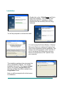


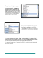
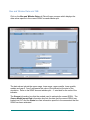


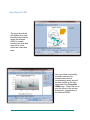

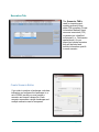


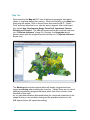
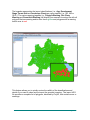
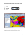
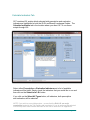
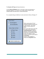
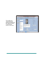


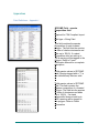
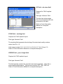


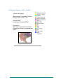
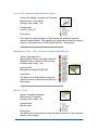


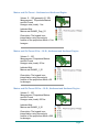
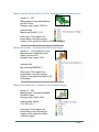

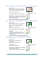
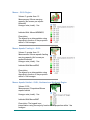


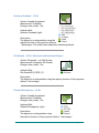


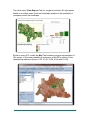


![Quick Start Guide - French [ 175093_FR ]](http://vs1.manualzilla.com/store/data/006343453_1-9600da95d2e1db5e232fd76b561e310c-150x150.png)