Download YIELD MONITOR DATA ANALYSIS

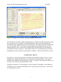
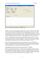
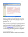
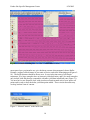
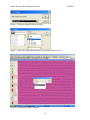
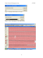
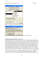
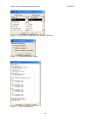
YIELD MONITOR DATA ANALYSIS: DATA ACQUISITION, MANAGEMENT, AND
ANALYSIS PROTOCOL
by
Terry W. Griffina, Jason P. Browna, and Jess Lowenberg-DeBoerb
a
Graduate Research Assistants and bProfessor
Version 1
August 2005
Department of Agricultural Economics
Purdue University
Purdue Site-Specific Management Center
8/30/2005
Table of Contents
Executive Summary ...................................................................................................................... 5
Overview of Spatial Analysis Steps ............................................................................................. 7
Yield Monitor Data Preparation ................................................................................................. 8
Discussion on using raw yield monitor data rather than filtering erroneous data ................ 8
Using the Yield Monitor’s Native Software with *.yld, *.gsy, *.gsd.................................. 10
AgLeader SMS Software from AgLeader.............................................................................. 10
JDOffice Software from John Deere..................................................................................... 11
Using Yield Monitor Data in absence of *.yld, *.gsy, *.gsd files........................................ 11
Data that has already been exported .................................................................................... 12
Using the manual export features of farm-level software..................................................... 12
Removing Erroneous Measurements ........................................................................................ 13
Assimilate Data with GIS ........................................................................................................... 16
Aggregating the dense data (yield) to the least dense data (i.e. soil points) ...................... 18
Creating buffer areal units for sparse data .......................................................................... 21
Assigning dense yield data to sparse data points ................................................................. 26
Appending treatment information to the dataset................................................................ 30
Adding the distance from a given attribute........................................................................... 31
Elevation, slope, aspect and associated problems................................................................ 32
Removing duplicate points.................................................................................................... 33
Spreadsheets ................................................................................................................................ 35
Exporting data from ArcView GIS for SpaceStat.................................................................. 39
Exploratory Spatial Data Analysis ............................................................................................ 39
Spatial Statistical Analysis ......................................................................................................... 46
Definition of regression analysis .......................................................................................... 47
Digression on appropriateness of spatial error and spatial lag models .............................. 49
Interpretation .............................................................................................................................. 50
Goodness-of-fit measurements not useful in spatial models................................................. 50
Goodness-of-fit measurements useful in spatial models....................................................... 51
Economic Analysis and Presentation of Results ...................................................................... 53
Disclaimers................................................................................................................................... 56
References.................................................................................................................................... 58
2
Purdue Site-Specific Management Center
8/30/2005
Yield Monitor Data Analysis: Data Acquisition, Management, and Analysis Protocol
Version 1 August 2005
Terry W. Griffina, Jason P. Browna, and Jess Lowenberg-DeBoerb
Graduate Research Assistants and bProfessor
Department of Agricultural Economics – Purdue University
a
Please send comments, suggestions and questions to:
Jess Lowenberg-DeBoer ([email protected]) 765.494.4230 or
Terry Griffin ([email protected]) 765.494.4257.
This document is currently available on-line and can be cited as:
Griffin, T.W., Brown, J.P., and Lowenberg-DeBoer, J. 2005. Yield Monitor Data Analysis:
Data Acquisition, Management, and Analysis Protocol. Available on-line at:
http://www.purdue.edu/ssmc
Executive Summary
This document serves to share our techniques for managing the analysis of site-specific
production data for the purposes of analyzing field-scale experiments. The content of this
document is the culmination of over a decade of on-farm trial and spatial analysis experience and
is still growing. The reader is invited to make suggestions and comments that may be
incorporated into future versions of this document.
This document also gives specifics on how to use spatial statistical analyses to analyze sitespecific yield monitor data rather than using traditional and albeit less efficient analysis. In the
presence of spatially variable data, traditional forms of analysis such as analysis of variance
(ANOVA) and least squares regression are unreliable and should be avoided. To our knowledge,
this document provides the most appropriate analysis methods for field-scale research with yield
monitor data.
Much of the following text and examples are useful for a wide range of precision agriculture
applications, but the overall thrust of this document is ultimately for analyzing field-scale
experiments. To conduct spatial analyses of yield monitor data both 1) a good experimental
design and 2) a planned comparison must be in place. A planned comparison can also be called
a testable question or testable hypothesis. If there is no hypothesis, neither traditional nor spatial
analysis can be conducted.
Although we recommend not using geostatistical interpolation techniques for conducting
inferential statistics, we do not make any statements on the use of these smoothing techniques for
prescription maps, defining management zones or other common uses.
The authors assume the reader has a working knowledge of MS Excel and ArcView GIS.
3
Purdue Site-Specific Management Center
8/30/2005
Overview of Spatial Analysis Steps
The following procedures describe the steps we take in data acquisition, management, and
analysis. The first portion of this procedure describes the methods we found that work the best
using publicly available software for data acquisition. In nearly all cases, yield monitor data
must be filtered before use in inferential analysis; thus a digression on data filtering is given.
Data assimilation and management with a geographical information system (GIS) is described
with several specific treatments of the data illustrated in detail. Data preparation for analysis is
explained using standard spreadsheets. The discussion on exploratory spatial data analysis
(ESDA) precedes the discussion on spatial statistical analysis. Finally, interpretation and
economic analyses are described.
Yield Monitor Data Preparation
This portion of the protocol is for preparing the dataset to be used in Yield Editor (USDA-ARS,
Columbia, MO) (Drummond, 2005) for removing erroneous data. Yield Editor can be
downloaded from the USDA-ARS website at:
http://www.fse.missouri.edu/ars/decision_aids.htm If Yield Editor is not being used, the reader
may skip directly to the section on GIS. According to Drummond’s (2005) criteria for importing
data, a few steps may need to be conducted to ensure the data is ready to be imported into Yield
Editor. This step is easiest if using the yield monitor’s native software package, however this is
not always possible especially for yield monitors from other than the major manufacturers. Both
scenarios are described.
It should be noted that these data preparation procedures may be referred to as “data cleaning” or
“data filtering” but actually are little more than removing measurements that are known to be
erroneous due to harvester machine dynamics and operator behavior. These data filtering
procedures are by no means a modification or manipulation of the data. Data filtering does
however increase the quality of the dataset.
Discussion on using raw yield monitor data rather than filtering erroneous data
Removing observations from a dataset without some sort of protocol has not been a commonly
accepted practice in statistics. Many analysts have omitted outliers by removing ±3 standard
deviations of the data or by plotting the data on a scattergram and removing obvious erroneous
data caused by factors such as human error, measurement error, or natural phenomena. With the
case of instantaneous yield monitor data, it is widely known that many observations have
erroneous yield values due to simple harvester machine dynamics. These erroneous observations
can be identified by examining harvester velocity, velocity change, maximum yield, and other
parameters. With harvester yield data, errors also arise from start and stop delays for beginning
and ending of passes. The ramping up and ramping down effects of the harvester yield monitor
has adverse effects on yield measurements. The flow delay caused by inaccurate assignment of
yield measurement to GPS coordinate is the effect of grain being harvested at one location, yield
measured while harvester is in another location, and recorded with GPS coordinates at
potentially another location. The flow delay must be corrected. If this error is not corrected,
yield values that are otherwise “good” are at the wrong location. Allowing native software
4
Purdue Site-Specific Management Center
8/30/2005
packages to impose the 12 second delay may be a good average, but we have typically seen
appropriate flow delays of six to 18 seconds but rarely exactly 12. Our assertion is that it is
dangerous to use raw yield monitor data for analysis, whether or not the native software performs
the default filtering and flow delay shifts. Conscious decision must be made as to the most
appropriate handing of the data. Some researchers have argued that data filtering is unethical
and prefer to accept data “as is” from the yield monitor, and thus from their farm-level software
regardless of the default filtering settings.
Using the Yield Monitor’s Native Software with *.yld, *.gsy, *.gsd
In packages such as JDOffice and AgLeader SMS the default setting import settings for start
delay, stop delay, and flow delay is typically 4, 4, and 12, respectively. It is our practice to set
these to zeros. If there is a minimum and maximum yield; we set these to zero and some value
near the maximum physical measurement of the yield monitor. These settings are chosen so that
the native software does not perform its “filtering” procedures so that more complete control is
possible during the filtering protocol. We do not perform any data manipulation procedures in
these native software packages other than a simple import and export of the yield monitor data.
SMS and JDOffice both have an automatic export function that exports yield monitor data in the
appropriate format.
AgLeader SMS Software from AgLeader
The current version of SMS (v5.5) unfortunately crashes when this export is performed, however
the procedure works in older and hopefully newer versions, thus is described here. (AgLeader
support has filed a “bug report”). For the mean time, an alternative approach is described in the
next section on “absence of native files” section. It should be noted that SMS does not have to
be a registered installation in order to perform the necessary procedures. Once the yield data has
been imported, export the data by File: Export: AgLeader Advanced Export.
JDOffice Software from John Deere
In order for the files to be exported in the appropriate format, a one time setting must be made.
Go to File:Preferences:Export and click the radio button next to “Text (comma delimited).” As
with SMS, JDOffice does not have to be registered. Once the yield layer of the field of interest
is active, go to File:Export:Layer Data.
Files exported by these SMS and JDOffice methods are ready for Yield Editor.
Using Yield Monitor Data in absence of *.yld, *.gsy, *.gsd files
Whether the data is already in the ArcView Shapefile format combination of *.shp, *.shx, *.dbf,
a georeferenced text file, or other file format, the data can usually be manually converted into the
appropriate *.txt file for Yield Editor pending having all the necessary data (columns). The
required data columns and arrangement are described in Drummond (2005).
Data that has already been exported
Using the *.dbf file portion of the Shapefile as exported from FarmWorks, SMS, JDOffice,
EasiSuite MapShots or other software package has been successful. Care must be taken to know
if the flow rates have been exported in kg per second or lbs per second, etc. as required by Yield
5
Purdue Site-Specific Management Center
8/30/2005
Editor (Drummond, 2005). Other measurements with metric or English units must also be
identified and converted to English units if necessary. Remaining data columns can be deleted.
Using the manual export features of farm-level software
We save a export template in SMS and FarmWorks (others may work, however we do not have
extensive experience with other farm-level software) when we export yield data so we can
quickly and easily export yield data in the future for Yield Editor.
This configuration can be saved by clicking Save Template. This template can be easily loaded
each time data is to be exported by clicking Load Template.
Removing Erroneous Measurements
Yield Editor 1.01 Beta (USDA-ARS) (Drummond, 2005) is used to remove erroneous data, i.e.,
filter the raw yield monitor data. Under a certain set of known harvester characteristics, the yield
monitor is unable to make accurate measurements. It is under these conditions that we use Yield
Editor to remove data points that are known to have been inaccurately measured.
Once a dataset is in the appropriate format as per the previous section, it can be imported into
Yield Editor (Figure 1). A user-defined or other standard protocol for filtering data can be
instated on the yield data but this is not recommended. The analyst’s intuition, experience, and
skill should guide the procedures. The data points are visually displayed so further manual
deletions can be made or points added back into the dataset if needed; thus this is an example of
where the analyst’s intuition is useful. The data filtering protocol may be farmer or field
specific. The best starting point is most likely zeros for all parameters, but this is dependent on
how data was managed during the import process in the native software, i.e. if flow delays were
allowed to be imposed on the data such as 4, 4, and 12 for start, stop, and flow delays,
respectively. However, conscious decisions must be made as to whether the protocols are
appropriate for the user’s application. It is our experience that no single parameter setting
structure is universally appropriate for any two fields, even with the same harvester and operator.
Adjusting flow delay, start pass delay, and end pass delay are the most difficult and may be the
most important to the quality of the data. End row yield points should be similar to adjacent end
row points. Differences are due to ramping up and down of the harvester at the beginning and
end of rows. Field experience indicates that it may take as much as 100 feet of harvester travel
before accurate yield measurements can be made. Adjust the delays until your intuition is
satisfied. (Values for the delays will typically be: Flow Delay 8 to 24, Start Pass Delay 0 to 10,
End Pass Delay 0 to 16; however variation occurs and parameters are set by trial-and-error plus
intuition). Negative values are possible. Setting the flow delay is easiest when the operator
harvests three to eight passes in one direction and alternates the pattern across the field. This
allows a visual reference wide enough to be seen on the Yield Editor map. Alternating direction
between individual passes does not give the needed visual reference.
6
Purdue Site-Specific Management Center
8/30/2005
Figure 1: Screenshot of Yield Editor Filtering, Mapping and Editing tab
Once the analyst is satisfied with the data filtering process and has recorded the parameters either
by saving the session or manually recording the parameter values in another document, the
filtered data can be exported into one of a few file formats. The authors typically export the data
as “space delimited ASCII” to facilitate less total steps before the import into ArcView GIS.
When prompted we place a check next to longitude (DD), latitude (DD), and yield under the
Save/Export File tab as in Figure 2. Some analysts choose to use UTM Easting (m) and UTM
Northing (m) in meters instead of decimal degree coordinates. Other data fields can be selected.
Assimilate Data with GIS
Open the new *.txt file exported from Yield Editor into WordPad, NotePad, or Excel. If using
WordPad or NotePad, add a blank line or row and name the column headings. The column
heading names should be separated with only a space. For instance, the columns would read: lat
long yield . Save this file as a tab delimited *.txt file.
If using Excel, open the *.txt file and specify “space delimited” if prompted. Add a blank row
and label the first, second, and third columns as lat, long, and yield, respectively. Save this file
as a tab delimited *.txt file.
7
Purdue Site-Specific Management Center
8/30/2005
Figure 2: Screenshot of Yield Editor Save/Export File tab
Add the *.txt file to your GIS package, for instance ArcView GIS or ArcMAP. From the Project
Window in ArcView GIS, select Table and click on Add. Navigate to the *.txt file. Go to the
View you wish to visualize your data and click View: Add Event Theme, specify the *.txt file
and assign the X and Y fields. Now that the *.txt file is loaded into the GIS, make sure it appears
correctly in the expected location with expected yield variation patterns similar to the variation in
the final Yield Editor map window (Figure 3). Depending upon which column variables you
selected in Yield Editor to export, your dataset will have differing pieces of data. At the very
least, you will have X and Y coordinates and the yield. The *.txt file will need to be converted
to a Shapefile format (Theme: Convert to Shapefile). Treatments, covariates, dummy variables
and topographical information will need to be added to this Shapefile in the GIS.
First, to return all inherent information, such as elevation, back to the new yield data file, a
spatial join is conducted appending pertinent information from the original yield data Shapefile
to the new yield Shapefile. The column fields that may be important to keep include elevation,
treatment information, and covariates such as electrical conductivity.
Aggregating the dense data (yield) to the least dense data (i.e. soil points)
Rarely ever does the differing data layers share the same spatial resolution or density, so some
sort of aggregation of the data is necessary. We have chosen the following process to minimize
the interference of the statistical reliability. Yield data is typically the most dense, followed by
soils such as Veris EC or other scouting information. Soil sampling for chemical analysis tends
to be the most sparsely collected data, such that it may be too sparse to even be
8
Purdue Site-Specific Management Center
8/30/2005
Figure 3: Screenshot of ArcView GIS of yield data exported from Yield Editor
included in the data. It has been our practice to keep the data in raw point format with the least
dense dataset to be the basis for the remaining data layers. We caution the analyst not to conduct
spatial interpolations via kriging or other geostatistical methods to remedy this dilemma. We
have avoided using geostatistical interpolation techniques for spatially smoothing a surface
because of the problem of introducing a random variable to the data, causing a problem in
deriving inference (Anselin, 2001).
There are a number of ways to assimilate yield data with the lesser dense soils data. Some sort
of spatial grid can be assigned to the dataset with each sparse soil data point being attributed to a
single grid unit. Our preferred method is to create a polygon with given radius with the soil
point as the center using the XTools (DeLaune, 2001) extension for Arcview GIS and is
explained in the folling paragraph. A specialized form of grid cells known as Thiessen polygons
can be created in GIS or GeoDa (University of Illinois) (Anselin, 2003). GeoDa can be
downloaded from: https://geoda.uiuc.edu/ and Thiessen polygons created by clicking
Tools:Shape:Points to Polygons. Thiessen polygons are a form of nearest neighbor interpolation
created by surrounding each input point with an areal unit such that any location within that area
is closer to the original point than any other point. Thiessen polygons are sometimes called or
very similar to Voronoi polygons, Delaunay Triangles, and Dirichlet Regions. A regular grid can
also be used, but it is difficult to line up irregular spaced data in a one-to-one format.
Creating buffer areal units for sparse data
With the ArcView GIS View projected with the distance units in the chosen units, go to XTools:
Buffer Selected Features (Figure 4) and choose the measurement unit of your choice, choose the
9
Purdue Site-Specific Management Center
8/30/2005
Figure 4: Screenshot showing ArcView GIS XTools Extension menu
most sparse layer you intend to use, give the theme a name when prompted, choose Buffer
Distance, assign a buffer distance in your units of choice, and select Noncontiguous (Figures 510). The buffer distance should be chosen as to 1) not overlap into areas of a different
treatments, 2) be large enough to have at least one yield observation, and 3) be small enough to
only include yield data that are comparable with other yield data in buffered zone (Figure 11).
You now have a new Shapefile layer with circular areal units around each of your sparse soil
points and is ready to have the dense yield data points added. These circular area units may
overlap, but that is not of concern.
Figure 5: Selected “meters” as the buffer unit
10
Purdue Site-Specific Management Center
8/30/2005
Figure 6: Select the Shapefile theme to buffer
Figure 7: Name the output Shapefile theme and assign location to save it
Figure 8: Selecting the “Buffer Distance”
11
Purdue Site-Specific Management Center
8/30/2005
Figure 9: Entering the buffer distance as 4.5 meters
Figure 10: Select “Noncontiguous” as the output structure
Figure 11: Screenshot of showing that the buffered areas do not cross treatments
12
Purdue Site-Specific Management Center
8/30/2005
Assigning dense yield data to sparse data points
Once polygon areal units have been created around the soils data, yield data can be assigned to
the soil location. The USGS Point Stat Calc (Dombroski) extension for ArcView GIS is useful
in simplifying this step (Figure 12). Select the dense yield data theme and the areal unit theme
for the less dense soils data as described in the previous discussions on buffered zones. Select
the value of interest for the point data (yield) as in Figure 13 and select all the statistics you wish
to use. We typically only use “Average”; however examining the standard deviation, coefficient
of variation, and other descriptive statistics gives an indication of the appropriateness of the
buffered distance for the given spatial variation.
Figure 12: Screenshot of USGS Point Stat Calc
After clicking “OK”, you will be prompted to provide a file name and decide whether you want
to create a new table or use the existing table. We typically accept all the default parameters as
shown in Figure 14. This step may take several minutes to a few hours depending on the size
and scale of the datasets. The new yield averages have been added to the buffer polygon theme.
Similar steps will need to be conducted to append the soils data to the soils buffered polygon
theme. These polygon areas need to be converted back into single points. This can be done
either 1) by using the original coordinates or 2) adding the centroid X and Y coordinate to the
dataset, opening the *.dbf of the buffered polygon theme with the Table command in the Project
window as described earlier in the section on adding the *.txt file from Yield Editor to ArcView
GIS (click Add Table in the Table portion of the Project Window and go to the View, click on
View from the main menu, click Add Event Theme, assign X and Y data, selecting the theme,
click Theme:Convert to Shapefile). Now the data for the dense and sparse data layers are in a
point data layer with the same resolution as the original sparse dataset and useful for inferential
statistics. Remember to convert each joined table to a Shapefile because joins with Point Stat
Calc are temporary joins and will be lost when another join is made.
13
Purdue Site-Specific Management Center
8/30/2005
Figure 13: Screenshot of Point Stat Calc input fields
Figure 14: Screenshot of Point Stat Calc “Create and Join Calculation Table”
Appending treatment information to the dataset
Treatment information may need to be added to the data file. If this information is not already
present in the dataset, it can be added in a number of ways. For instance, if the treatments occur
in blocks like tillage treatments or split field trials, polygons can be created and merged together
to form the treatment polygon map. From this polygon, a specific treatment can be selected.
Once the treatment is selected from the treatment polygon map, a Select by Theme can be done
on the yield data points with respect to the selected portion of the treatment polygon map. Now
that the yield data points associated with the treatment are selected, a dummy variable can be
added using the SpaceStat Extension to ArcView GIS (TerraSeer) (Anselin, 1999). To add a
dummy variable, click Data, Add Dummy and give an appropriate name. A “1” is added in this
column for selected features and a “0” otherwise. These same steps can be done to add a dummy
for soil series, other regions such as old feedlots, pastures, homesteads, and two existing fields
were joined to be one large field. A dummy variable should be added for each categorical
treatment, soil zone, and every measurable discrete factor to be included in the statistical model.
14
Purdue Site-Specific Management Center
8/30/2005
Adding the distance from a given attribute
In some cases, a distance variable may be useful to help describe variability from isotropic or
anisotropic effects. In cases of furrow irrigation where plants near the water canal will surely get
more water, albeit colder water, than plants at the other end of the row, differing yield responses
are expected. Distances are also useful in modeling the isotropic effect of flood irrigated rice
production where plants near the water source tend to have lower yields due to the colder
temperature of the ground water near the well. The distance to the given attribute can be added
to the dataset in a number of ways. One method involves using the Distance Matrix extension
for ArcView GIS (Jenness, 2005a). The output from Distance Matrix can be joined into the
existing dataset by the standard table joining techniques in ArcView GIS.
Elevation, slope, aspect and associated problems
Due to introduction of variability problems associated with geostatistical techniques (Isaaks and
Srivastava, 1989) and imperfect information on proper parameters to assign to interpolation
methods, spatial interpolation methods such as inverse distance weighting, kriging, and cokriging have been avoided. However, if slope or aspect variables are desired, the elevation data
must be interpolated into a surface. In addition, the elevation data must be collected at a
resolution sufficient to describe the topography and with adequate accuracy. Tractors equipped
with RTK automated guidance typically provide sufficient data during plating or other field
operations. Coast Guard and WAAS DGPS do not always provide the needed accuracy.
Additional data points and resolution are not substitutes for accuracy.
From this elevation surface a slope, aspect, or other topographic surface can be calculated. The
slope surface can be converted into a contour line vector with base of zero and interval of 0.25
percent. The yield data can be appended with a value for slope by choosing the closest slope
contour line by using the Spatial Join function in Geostatistical Wizard in ArcView GIS. The
danger in spatial interpolation of a surface is the introduction of variability or in other words
introducing a random variable which causes problems with statistical inference (Anselin, 2001).
Removing duplicate points
It may be necessary to remove duplicate points in the data. For instance, GeoDa does not allow
points with the same coordinate. If this is a problem, the Find Duplicate Shapes or Records
extension (Jenness, 2005b) can be used in ArcView GIS. When using this extension, the analyst
is asked to give the name of the theme and unique identifier (Figure 15), the criteria for defining
duplicates (Figure 16), and is provided a report of the duplicated points and which points were
removed (Figure 17). Adding an unique identifier is discussed later in the section on
spreadsheets.
15
Purdue Site-Specific Management Center
8/30/2005
Figure 15: Screenshot of Find Duplicate Shapes or Records
Figure 16: Selecting duplicate criteria
Figure 17: Report on duplicates
16
Purdue Site-Specific Management Center
8/30/2005
Spreadsheets
Once the dataset has all the necessary GIS work, a spreadsheet such as MS Excel is useful for
calculating additional variables. These variables may include interaction terms, dummy
variables of differing coding, squaring continuous explanatory variables, and a unique identifier
field if one has not already been created. The unique ID field is required by GeoDa and many
GIS functions. We typically add a column and name it with our initials, an underscore, and “ID”
so “TWG_ID” is my brand. Some analysts use “POLYID” by convention. Then a sequential set
of numbers are added to uniquely identify each row of data or record.
For the purposes of regression analysis, some variables must be squared, cubed, square root,
natural log, or other transformation. For most studies, the original variable plus a squared term is
sufficient if the variable is supporting information. If the variable is the experimental treatments,
cubed and other higher order transformations are needed depending upon the model.
Once all the main variables are created and exist in the spreadsheet, interaction terms of all the
explanatory variables should be created that are intended to be used in the full model. The most
important interaction terms are the factors with each other if there is more than one factor.
Interaction terms of the factor with other variables such as elevation, soil zone, dummy variable,
or other covariates are also useful. This allows each major measured yield affecting factor to
have its own slope and intercept.
For categorical treatments and supporting variables such as soil zones, hybrids, or other discrete
choices, a binary or dummy variable should be created. For instance, any observation that is
present in soil A has a “1” with other observations having a “0” as outlined in a previous section.
To make the regression comparable to ANOVA and to have the coefficients presented as the
difference from average conditions, a restriction on the dummy variables that they sum to zero
can be imposed (∑ d ij = 0 ) . This can be done when there are two or more categories. When
there are three or more dummy variables, the convention is to select one treatment to be the
reference. The process for assigning dummy variables is now to subtract the value of the
reference from the remaining categories. This method generates a “-1” if the observation is of
the reference category, a “1” for an observation from the category in question and a “0”
otherwise. When the regression is run, the reference category is dropped from the analysis and is
captured in the intercept. When the dummy variables are coded in this way, all coefficients are
evaluated at mean conditions.
When working with large spreadsheets having thousands of rows of data, knowing shortcut
methods can save a lot of time. For instance, if the user wants to highlight from the active cell to
the last row of data in the spreadsheet, press and hold Control and Shift and then press the down
arrow. Remember when using formulas to fill in data, that the formulas need to be saved as
values so the resulting *.dbf or *.txt files operate properly. When working with a *.dbf and the
user wants to create new columns, it is easiest to insert a new column in the middle of the data
with existing data columns to the right. Otherwise, the file may not save the new columns if they
are to the right of the existing data. In addition, using a *.dbf may not save the number of
decimal places and revert to an integer, causing difficulties when dealing with many types of
data or even coordinate systems. It is a good practice to first save the spreadsheet as the native
17
Purdue Site-Specific Management Center
8/30/2005
*.xls file and then perform a “save as” to the *.dbf or *.txt so that a clean backup is available.
The analyst should avoid sorting this file unless care is taken to sort the data in a specific manner
to be able to resort the data to the original sequence of data rows. The best way to sort the data is
to have a unique identifier column that has a sequential order. The whole dataset except for
column headings must be sorted all at once. Before saving the dataset file, the whole dataset
must be sorted back to the original sequence by using the unique identifier column. If the rows
of data get arranged in an inappropriate manner, the GIS software still operates properly however
the data does not match the appropriate shape. In other words all the data is present, but is
associated with the wrong location. Likewise, the analyst must not delete rows of data in the
spreadsheet because the GIS software will not accept the Shapefile.
Exporting data from ArcView GIS for SpaceStat
Once the appropriate variables have been created in the spreadsheet, added to ArcView GIS, and
converted to a Shapefile, it can be exported in the appropriate format for spatial statistical
analysis in SpaceStat by using the SpaceStat extension (Anselin, 1999) to ArcView GIS by
clicking Data: Table to SpaceStat Data Set. SpaceStat can be purchased from TerraSeer
(http://www.terraseer.com/).
Exploratory Spatial Data Analysis
“In exploratory spatial data analysis, one should not rigidly follow a prescribed sequence of
steps but should, instead, follow one’s instinct for explaining anomalies” (Isaaks and Srivastava,
page 525). This leads to an underlying assumption in spatial analysis, that the analyst either has
intimate knowledge of the field or is in close contact with a collaborator who does, i.e. the
farmer. The results of exploratory spatial data analysis (ESDA), and steps the analyst takes to
arrive at these results, are intended to give the analyst a better understanding of the spatial
variation of the data.
Now that the entire dataset is in a single Shapefile, ESDA can be performed using GeoDa. Open
a file using the standard icons and navigate to the folder where the Shapefile is being kept.
GeoDa asks that a unique identifier be assigned and is referred to as a key variable (Figure 18).
To perform any ESDA, a weights matrix must be specified. This can be done by clicking
Tools:Weights:Create. The resulting box (Figure 19) asks an input file (which will probably be
the same Shapefile), a name for the weights matrix (in this case W_min) and the key variable
again. In this example we chose to have an Euclidean distance with a cutoff of 7.169765 meters,
the minimum distance such that each observation has at least one neighbor which can be
determined when the sliding bar is all the way to the left.
Figure 18: Selecting a GeoDa project and assigning the key variable
18
Purdue Site-Specific Management Center
8/30/2005
Figure 19: Creating a weights matrix in GeoDa
In order for GeoDa to display the distance in meters or any other specified unit, the Shapefile
should be exported in some projection other than decimal degrees. This can be done in
ArcView GIS by clicking Theme:Convert to Shapefile and then select the option to maintain the
projection. Whatever projection that the View is projected will be the units GeoDa displays.
Otherwise if the Shapefile is exported without the projection, the units will be in decimal degrees
and difficult to interpret.
One statistical measure of spatial variability is Moran’s I (Anselin, 1988; Cliff and Ord, 1981).
Moran’s I is a global indicator of spatial autocorrelation. To calculate and plot the data for
Moran’s I, go to Space:Univariate Moran and select the variable you wish to explore (Figure 20).
You will be asked to provide a weights matrix to use which you just created (Figure 21). The
resulting Moran’s I scatter plot and value (Figure 22) gives indication to the amount of spatial
autocorrelation. In all the site-specific data that we have used, we typically expect to have
positive values and not negative or zero values at field-scales.
Now that the analyst has a firm understanding of the spatial variation of the dataset, the analyst is
ready to conduct statistical analyses.
19
Purdue Site-Specific Management Center
8/30/2005
Figure 20: Selecting the YLD02 variable to calculate a Moran’s I
Figure 21: Assigning a weights matrix in GeoDa
20
Purdue Site-Specific Management Center
8/30/2005
Figure 22: A Moran’s I for YLD02 variable
Spatial Statistical Analysis
Traditional analyses such as ANOVA and ordinary least squares regression are unreliable in the
presence of spatial variability or in other words spatial autocorrelation and spatial
heteroskedasticity. The assumption of independent observations, normality, and identically and
independently distributed (iid) errors are all violated. Spatial regression analysis is one
methodology that overcomes these limitations of traditional analyses (see Anselin {1988} or
Cressie {1993} for a thorough treatment of spatial statistical methodologies).
Definition of regression analysis
Regression analysis defined in the traditional sense can be thought of as a model-driven
functional relationship between correlated variables that can be estimated from a given dataset.
Regression can be used to predict values of one variable when given values of the others. Spatial
statistics expands upon traditional regression to address the problems of spatial dependence,
specifically in the form of spatial autocorrelation, and spatial heterogeneity (Anselin,1988). Any
appropriate statistical analysis of a spatial dataset can be thought of as spatial statistics.
GeoDa provides an ordinary least squares (OLS) and two spatial regression methods both using
maximum likelihood (ML) estimation. OLS regression is necessary for the purpose of
conducting spatial diagnostics on the OLS residuals to determine whether a spatial regression
method is justified and which of the two methods is the most appropriate. If the diagnostics of
21
Purdue Site-Specific Management Center
8/30/2005
the residuals suggests a spatial method is appropriate, either a spatial error or a spatial lag model
will be indicated that best describes the data. From our experience with field-scale on-farm data,
the diagnostics indicate a spatial error model most of the time. GeoDa presents spatial
diagnostics including Lagrange Multiplier (LM) values and Robust LM values for both spatial
error and spatial lag. The diagnostic values with the largest LM and Robust LM values, or
smallest probability levels, is the most appropriate to use. In most cases, both the LM and
Robust LM diagnostics indicate the same model; however differing indicators may mean that
simultaneously both are appropriate. In some cases, the Spatial Autoregressive Moving Average
(SARMA) may be the most appropriate as indicated by the diagnostics, however estimation is
considerably more complicated and no clear interpretation exists. In examining the SARMA
diagnostic, the analyst is cautioned not to compare the LM values directly because SARMA is
distributed χ 22 (chi-squared with two degrees of freedom) and LM is distributed χ 12 (chi-squared
with one degree of freedom). In addition, there is some conceptual evidence that the spatial
error model is more appropriate than the spatial lag model; however some disagreement by
researchers exists as described in the digression on spatial statistical methods below.
Digression on appropriateness of spatial error and spatial lag models
Debates over which spatial model is most appropriate for site-specific data are still on-going
between practitioners and theorists. It is our position that the spatial error model is conceptually
the most appropriate for field-scale data. Conceptually, the spatial error model tends to be the
most appropriate model when the spatial structure is explained in the residuals of the regression,
or in other words due to omitting variables that explain the yield variability. Yield variability at
field-scales occurs for several factors, and most are not measured and therefore cannot be
included in the statistical model. When the statistical model is run without the yield variability
factors being included, the unanswered variability inevitably winds up in the residuals or error
term making the spatial error model the most appropriate. It is doubtful that researchers and
farmers will collect the exact data at the resolution needed to overcome the omitted variable
problem, even with dense soil data such as electrical conductivity. Conversely, the spatial lag
model is conceptually the most appropriate model when the spatial variability occurs in the
predicted dependent variable itself, and in our case crop yield. In situations where the dependent
variables affect each other directly instead of being affected by an underlying mechanism, the
spatial lag model is appropriate. These situations may include any contagion such as property
values from regional economics and disease spread in epidemiology. These factors affect and
are affected by one another. It is counterintuitive to suggest that high crop yields in one location
cause crop yields in adjoining locations to be high and vice versa. However, from statistical
theory we know that the spatial lag model accounts for spatial autocorrelation in both the
dependent variable and error terms. This has caused some theorists to suggest that the spatial lag
model is most appropriate. This is an open debate and we welcome your thoughts and
experiences on this topic.
Interpretation
Spatial regression techniques may someday become commonplace to the farmer or farm
consultant, but currently university researchers are still developing the methodology. For the
time being, spatial analysts who invest a portion of their time to teach the ultimate end user of
this technology, the farm manager, to interpret analysis results rather than conduct the intricate
22
Purdue Site-Specific Management Center
8/30/2005
details may have made considerable contributions to spatial analysis (Griffin and Lambert,
2005).
Goodness-of-fit measurements not useful in spatial models
In traditional analyses, the R-squared statistic is a common measure of ‘goodness-of-fit’ or the
adequacy of the model. The R-squared statistic ranges from zero, meaning it explains none of
the variability in the data, to one, meaning the model explains 100% of the data. R-squared
values somewhere between zero and one are expected. Although OLS models report R-squared
even with spatial data, the value is meaningless. For instance, Griffin et al. (2004) showed that
OLS models were unable to adequately explain spatial datasets under simulation; however the Rsquared values and F-statistics were very high. If spatial diagnostics on the OLS residuals
indicated the presence of spatial autocorrelation, then the OLS coefficients, standard errors, and
goodness-of-fit statistics for OLS should be ignored. In addition, R-squared values do not have
the same interpretation with a spatial model as the OLS model and are normally assumed to be
invalid (Anselin, 1988).
Goodness-of-fit measurements useful in spatial models
A better goodness-of-fit measurement is the maximized log-likelihood. The use of traditional
measures such as chi-squared and mean squared error provide misleading results with spatial
models (Anselin, 1988). The Akaike Information Criterion (AIC) estimates the expected value
of the Kullback-Leibler information criterion (KLIC) which has an unknown distribution
(Anselin, 1988). The ranking of models by AIC is useful although the specific value has little
meaning. The analyst should examine several goodness-of-fit measurements and not make
judgments based on a single measure.
With spatial error models, the coefficients, standard errors, z-value, and probability has similar
interpretation as OLS, with the z-value corresponding to the t-value. Asymptotically, the
absolute value of the z-value will be greater than or equal to 1.96 to be significant at the 5%
confidence level. The probability level will be 0.05 for the 5% level meaning that we expect to
be wrong 5% of the time. Although confidence levels such as 1%, 5%, and 10% are chosen by
convention, the analyst is able to set their own requirements for confidence. The analyst should
be cautioned that while the regression results from spatial error models can be directly compared
to least squares and ANOVA, spatial lag model regression coefficients must be adjusted using an
infinite series expansion adjustment.
A regression model can possess independent variables that are solely dummy variables. These
models are commonly referred as analysis of variance (ANOVA) models. If the ANOVA coding
is used as described in a previous section on Spreadsheets where the restriction that dummy
variables sum to zero (∑ d ij = 0 ) is imposed, the analyst should be aware that the reported pvalues represent the model at the average conditions, and not at the intercept. This is
mathematically identical to ANOVA; however field-scale research typically has a wide range of
soils, topography, and other yield influence factors. When ANOVA is used with small-plot
experiments, the average condition of the plots is very similar to any given plot. At field-scales,
the average condition probably does not closely describe the majority of locations in the field
and the analyst must understand that the p-values may differ at differing locations in the field
(i.e. soil clay content, organic matter level, elevation, etc.).
23
Purdue Site-Specific Management Center
8/30/2005
Economic Analysis and Presentation of Results
It is our practice to take the regression results and graph them so that the results can be easily
communicated with decision makers. Once the regression output is available, copy and paste the
output to a spreadsheet. It may be necessary to click Data: Text to Columns to nicely fit the data
into the spreadsheet cells. From the coefficients, we calculate the dependent variable, typically
yield, over a range of the covariates such as clay content, elevation, or other continuous variables
for each treatment and/or other discrete categories such as soils (see Figure 23 for example).
From these calculations, we create a XY(Scatterplot). These graphs are useful in discussing and
interpreting the results of the planned comparison with the farm management decision-maker.
For rudimentary economic analysis of side-by-side or categorical treatments, a partial budget
will suffice. A partial budget includes only the costs and revenues that differ from alternative to
alternative, while an enterprise budget is exhaustive. For field-scale experiments, the difference
in revenue may only include the difference in revenue for each treatment, or R = p y y where R is
revenue, py is price of crop, and y is the crop yield. The difference in costs may include the seed
costs if a hybrid trial or the machinery costs if a tillage trial.
For rate trails such as nitrogen rates or seeding rates, the equation derived from the regression
model is used. For instance with soybean seeding rates, the equation may be
y s = pop + pop 2 + elev where ys is soybean yield, pop and pop2 are seeding population and
population squared, and elev is the elevation. The model coefficients are used to calculate yield
maximizing soybean population levels, or what is commonly known as agronomic maximum.
However, yield maximized levels are not profit maximization levels unless the soybean seed is
free, an unlikely situation. To calculate profit maximization levels, or economic optimal levels,
the profit function must be used π = R − C where π is profit, R is revenue and C is cost. The
profit function can be expanded to π = p y y − px x where px is the price of the input, x. So the
equation for profit from a soybean population rate study may be
π s = p y ( pop + pop 2 + elev ) − ps ( pop ) where π s is profit from soybean and ps is the price of
soybean seed. Yield maximization and profit maximization levels can be found in the above
examples by taking the first derivative and solving for the input. For instance, the profit
maximization level can be solved for the research factor from the above equation by
ps − p y
pop =
. The above examples are only one of a large number of possibilities for models
2 py
and research factors. Each planned comparison may have a completely different model, costs,
and treatments and the analyst should be prepared to adjust their own protocol accordingly.
24
Purdue Site-Specific Management Center
8/30/2005
Site Specific Spatial Error Estimated Yield Response to Seeding Rate
70
65
Yield (Bu/Acre)
60
55
50
45
40
35
70
80
90
100
110
120
130
140
150
160
170
Seed Population (Thousands/Acre)
Avg. Elev. & Slope
Low Elev. & Slope
High Elev. & Slope
Low Elev. & High Slope
High Elev. & Low Slope
Figure 23: Example graph of results from soybean seeding rate study by regime
Disclaimers
The purpose of this document is to provide a suggestion on using yield monitor data and spatial
analysis methods in evaluation of treatments from farm-level field-scale experiments. The
opinions and conclusions expressed here are those of the authors. Mention of specific suppliers
of hardware and software in this manuscript is for informative purposes only and does not imply
endorsement.
Note on ArcView Extensions
I will try to keep a decent list of links to useful ArcView GIS extensions on my website at:
http://web.ics.purdue.edu/~twgriffi/av_extensions.html
25
Purdue Site-Specific Management Center
8/30/2005
References
AgLeader SMS http://www.agleader.com/sms.htm
Anselin, L. 1988. Spatial Econometrics: Methods and Models, Kluwer Academic Publishers,
Drodrecht, Netherlands.
Anselin, L. 1992. SpaceStat Tutorial. University of Illinois, Urbana-Champaign, Urbana, IL
61801. http://www.terraseer.com
Anselin, L. 1999. Spatial Data Analysis with SpaceStat and ArcView Workbook 3rd Ed.
Available on-line at: http://www.terraseer.com/products/spacestat/docs/workbook.pdf
Anselin, L. 2001. Spatial Effects in Econometric Practice in Environmental and Resource
Economics, American Journal of Agricultural Economics 83, 705-710.
Anselin, L. 2003. GeoDa 0.9 User's Guide. Spatial Analysis Laboratory, University of Illinois,
Urbana-Champaign, IL. http://sal.agecon.uiuc.edu/geoda_main.php
Cliff, A.D. and Ord, J.K. 1981. Spatial Processes, Models and Appplications. London: Pion.
Cressie, N. A.C. 1993. Statistics for Spatial Data. John Wiley & Sons: New York.
DeLaune, Mike. Guide to XTools Extension. September 2003. Available on-line at:
http://www.odf.state.or.us/divisions/management/state_forests/XTools.asp
Dombroski, Mathew. ESRI ArcView Extension: Point Stat Calc. Available on-line at:
http://pubs.usgs.gov/of/of00-302/
Drummond, Scott. 2005. Yield Editor 1.00 Beta Version User’s Manual November 9, 2004.
http://www.fse.missouri.edu/ars/ye/yield_editor_manual.pdf
JDOffice http://www.deere.com/en_US/ag/servicesupport/ams/JDOffice.html Deere and
Company, Moline, IL.
Griffin, T.W., D.M. Lambert and J. Lowenberg-DeBoer, 2004. “Testing for Appropriate OnFarm Trial Designs and Statistical Methods for Precision Farming: A Simulation Approach.”
Forthcoming in 2005 Proceedings of the 7th International Conference on Precision Agriculture
and Other Precision Resources Management, ASA/SSSA/CSSA, Madison, Wisconsin.
Griffin, Terry and Dayton Lambert. 2005. Teaching Interpretation of Yield Monitor Data
Analysis: Lessons Learned from Purdue's 37th Top Farmer Crop Workshop. Journal of
Extension 23(3).
Isaaks, E.H. and Srivastava, R.M. 1989. An Introduction to Applied Geostatistics. Oxford
University Press, Inc. New York, NY.
26
Purdue Site-Specific Management Center
8/30/2005
Jenness, J. 2005a. Distance Matrix (dist_mat_jen.avx) extension for ArcView 3.x, v. 2. Jenness
Enterprises. Available at: http://www.jennessent.com/arcview/dist_matrix.htm.
Jenness, J. 2005b. Find Duplicate Shapes or Records (find_dupes.avx) extension for ArcView
3.x, v. 1.1. Jenness Enterprises. Available at:
http://www.jennessent.com/arcview/find_dupes.htm.
Littell, R.C., G.A. Milliken, W.W. Stroup, R.D. Wolfinger. 1996. SAS System for Mixed
Models. The SAS Institute Inc., Cary, North Carolina.
DeLaune, Mike. Guide To XTools Extension September 2003. Available on-line at:
http://www.odf.state.or.us/divisions/management/state_forests/XTools.asp
27