1
PHITS
Ver. 2.30
User’s Manual
English version
Contents
1
Introduction
1.1 Recent technical notice . . . . . . . . . . . . . . . . . . . . . . . . . . . . . . . . . . . . . . . .
1.2 Development members . . . . . . . . . . . . . . . . . . . . . . . . . . . . . . . . . . . . . . . .
2
Models implemented in the code
2.1 JAM model . . . . . . . . . . . . . . . . . . . . . . . . . . . . . . . . . . . .
2.1.1 Main feature of JAM . . . . . . . . . . . . . . . . . . . . . . . . . . .
2.1.2 Elementary cross sections of hadron-hadron . . . . . . . . . . . . . . .
2.2 JQMD model . . . . . . . . . . . . . . . . . . . . . . . . . . . . . . . . . . .
2.3 New features of PH I TS . . . . . . . . . . . . . . . . . . . . . . . . . . . . . .
2.3.1 Event generator mode for low energy neutron incident reactions . . . .
2.3.2 Microscopic approach for estimation of relative biological effectiveness
.
.
.
.
.
.
.
.
.
.
.
.
.
.
.
.
.
.
.
.
.
.
.
.
.
.
.
.
.
.
.
.
.
.
.
.
.
.
.
.
.
.
.
.
.
.
.
.
.
.
.
.
.
.
.
.
.
.
.
.
.
.
.
.
.
.
.
.
.
.
3
3
3
4
7
10
10
10
Installation
3.1 Source files and data files .
3.2 Compiling the PH I TS code
3.3 Compiling AN GE L . . . .
3.4 Executable file . . . . . .
3.5 Terminating PH I TS code .
3.6 Array sizes . . . . . . . .
3
4
5
1
1
2
.
.
.
.
.
.
.
.
.
.
.
.
.
.
.
.
.
.
.
.
.
.
.
.
.
.
.
.
.
.
.
.
.
.
.
.
.
.
.
.
.
.
.
.
.
.
.
.
.
.
.
.
.
.
.
.
.
.
.
.
.
.
.
.
.
.
.
.
.
.
.
.
.
.
.
.
.
.
.
.
.
.
.
.
.
.
.
.
.
.
.
.
.
.
.
.
.
.
.
.
.
.
.
.
.
.
.
.
.
.
.
.
.
.
.
.
.
.
.
.
.
.
.
.
.
.
.
.
.
.
.
.
.
.
.
.
.
.
.
.
.
.
.
.
.
.
.
.
.
.
.
.
.
.
.
.
.
.
.
.
.
.
.
.
.
.
.
.
.
.
.
.
.
.
.
.
.
.
.
.
.
.
.
.
.
.
.
.
.
.
.
.
.
.
.
.
.
.
.
.
.
.
.
.
.
.
.
.
.
.
.
.
.
.
.
.
12
12
13
13
13
14
15
Input File
4.1 Sections . . . . . . . . . . . . .
4.2 Reading control . . . . . . . . .
4.3 Inserting files . . . . . . . . . .
4.4 User definition constant . . . . .
4.5 Using mathematical expressions
4.6 Using the CG or GG . . . . . .
4.7 Particle identification . . . . . .
.
.
.
.
.
.
.
.
.
.
.
.
.
.
.
.
.
.
.
.
.
.
.
.
.
.
.
.
.
.
.
.
.
.
.
.
.
.
.
.
.
.
.
.
.
.
.
.
.
.
.
.
.
.
.
.
.
.
.
.
.
.
.
.
.
.
.
.
.
.
.
.
.
.
.
.
.
.
.
.
.
.
.
.
.
.
.
.
.
.
.
.
.
.
.
.
.
.
.
.
.
.
.
.
.
.
.
.
.
.
.
.
.
.
.
.
.
.
.
.
.
.
.
.
.
.
.
.
.
.
.
.
.
.
.
.
.
.
.
.
.
.
.
.
.
.
.
.
.
.
.
.
.
.
.
.
.
.
.
.
.
.
.
.
.
.
.
.
.
.
.
.
.
.
.
.
.
.
.
.
.
.
.
.
.
.
.
.
.
.
.
.
.
.
.
.
.
.
.
.
.
.
.
.
.
.
.
.
.
.
.
.
.
.
.
.
.
.
.
.
.
.
.
.
.
.
.
.
.
.
.
.
.
.
.
.
.
.
.
.
.
.
.
.
.
16
16
17
18
18
18
19
19
Sections format
5.1 [ T i t l e ] section . . . . . . . . . . . . . . . . . . . . .
5.2 [ P a r a m e t e r s ] section . . . . . . . . . . . . . . . .
5.2.1 Calculation mode . . . . . . . . . . . . . . . . .
5.2.2 Number of history and Bank . . . . . . . . . . .
5.2.3 Cut off energy and switching energy . . . . . . .
5.2.4 Cut off time, cut off weight, and weight window .
5.2.5 Model option (1) . . . . . . . . . . . . . . . . .
5.2.6 Model option (2) . . . . . . . . . . . . . . . . .
5.2.7 Model option (3) . . . . . . . . . . . . . . . . .
5.2.8 Output options (1) . . . . . . . . . . . . . . . .
5.2.9 Output option (2) . . . . . . . . . . . . . . . . .
5.2.10 Output option (3) . . . . . . . . . . . . . . . . .
5.2.11 Output option (4) . . . . . . . . . . . . . . . . .
5.2.12 About geometrical errors . . . . . . . . . . . . .
5.2.13 Input-output file name . . . . . . . . . . . . . .
5.2.14 Others . . . . . . . . . . . . . . . . . . . . . . .
5.2.15 Physical parameters for low energy neutron . . .
5.2.16 Physical parameters for photon . . . . . . . . . .
5.2.17 Physical parameters for electron . . . . . . . . .
5.2.18 Dumpall option . . . . . . . . . . . . . . . . . .
5.2.19 Event Generator Mode . . . . . . . . . . . . . .
5.3 [ S o u r c e ] section . . . . . . . . . . . . . . . . . . .
5.3.1 <Source> : Multi-source . . . . . . . . . . . . .
5.3.2 Common parameters . . . . . . . . . . . . . . .
.
.
.
.
.
.
.
.
.
.
.
.
.
.
.
.
.
.
.
.
.
.
.
.
.
.
.
.
.
.
.
.
.
.
.
.
.
.
.
.
.
.
.
.
.
.
.
.
.
.
.
.
.
.
.
.
.
.
.
.
.
.
.
.
.
.
.
.
.
.
.
.
.
.
.
.
.
.
.
.
.
.
.
.
.
.
.
.
.
.
.
.
.
.
.
.
.
.
.
.
.
.
.
.
.
.
.
.
.
.
.
.
.
.
.
.
.
.
.
.
.
.
.
.
.
.
.
.
.
.
.
.
.
.
.
.
.
.
.
.
.
.
.
.
.
.
.
.
.
.
.
.
.
.
.
.
.
.
.
.
.
.
.
.
.
.
.
.
.
.
.
.
.
.
.
.
.
.
.
.
.
.
.
.
.
.
.
.
.
.
.
.
.
.
.
.
.
.
.
.
.
.
.
.
.
.
.
.
.
.
.
.
.
.
.
.
.
.
.
.
.
.
.
.
.
.
.
.
.
.
.
.
.
.
.
.
.
.
.
.
.
.
.
.
.
.
.
.
.
.
.
.
.
.
.
.
.
.
.
.
.
.
.
.
.
.
.
.
.
.
.
.
.
.
.
.
.
.
.
.
.
.
.
.
.
.
.
.
.
.
.
.
.
.
.
.
.
.
.
.
.
.
.
.
.
.
.
.
.
.
.
.
.
.
.
.
.
.
.
.
.
.
.
.
.
.
.
.
.
.
.
.
.
.
.
.
.
.
.
.
.
.
.
.
.
.
.
.
.
.
.
.
.
.
.
.
.
.
.
.
.
.
.
.
.
.
.
.
.
.
.
.
.
.
.
.
.
.
.
.
.
.
.
.
.
.
.
.
.
.
.
.
.
.
.
.
.
.
.
.
.
.
.
.
.
.
.
.
.
.
.
.
.
.
.
.
.
.
.
.
.
.
.
.
.
.
.
.
.
.
.
.
.
.
.
.
.
.
.
.
.
.
.
.
.
.
.
.
.
.
.
.
.
.
.
.
.
.
.
.
.
.
.
.
.
.
.
.
.
.
.
.
.
.
.
.
.
.
.
.
.
.
.
.
.
.
.
.
.
.
.
.
.
.
.
.
.
.
.
.
.
.
.
.
.
.
.
.
.
.
.
.
.
.
.
.
.
.
.
.
.
.
.
.
.
.
.
.
21
21
21
22
22
23
24
25
26
27
28
29
30
31
32
32
33
34
34
35
36
39
40
40
41
.
.
.
.
.
.
.
.
.
.
.
.
ii
5.4
5.5
5.6
5.7
5.8
5.9
5.10
5.11
5.12
5.13
5.14
5.15
5.16
5.17
5.18
5.19
5.3.3 Cylinder distribution source . . . . . . . . . . . . . . .
5.3.4 Rectangular solid distribution source . . . . . . . . . . .
5.3.5 Gaussian distribution source (x,y,z independent) . . . .
5.3.6 Generic parabola distribution source (x,y,z independent)
5.3.7 Gaussian distribution source (x-y plane) . . . . . . . . .
5.3.8 Generic parabola distribution source (x-y plane) . . . . .
5.3.9 Sphere and spherical shell distribution source . . . . . .
5.3.10 s-type = 11 . . . . . . . . . . . . . . . . . . . . . . . .
5.3.11 s-type = 12 . . . . . . . . . . . . . . . . . . . . . . . .
5.3.12 Reading dump file . . . . . . . . . . . . . . . . . . . .
5.3.13 User definition source . . . . . . . . . . . . . . . . . .
5.3.14 Definition for energy distribution . . . . . . . . . . . .
5.3.15 Definition for angular distribution . . . . . . . . . . . .
5.3.16 Example of multi-source . . . . . . . . . . . . . . . . .
5.3.17 Duct source option . . . . . . . . . . . . . . . . . . . .
[ M a t e r i a l ] section . . . . . . . . . . . . . . . . . . . . . .
5.4.1 Formats . . . . . . . . . . . . . . . . . . . . . . . . . .
5.4.2 Nuclide definition . . . . . . . . . . . . . . . . . . . .
5.4.3 Density definition . . . . . . . . . . . . . . . . . . . . .
5.4.4 Material parameters . . . . . . . . . . . . . . . . . . .
5.4.5 S (α, β) settings . . . . . . . . . . . . . . . . . . . . . .
5.4.6 Examples . . . . . . . . . . . . . . . . . . . . . . . . .
[ B o d y ] section . . . . . . . . . . . . . . . . . . . . . . . . .
5.5.1 formats . . . . . . . . . . . . . . . . . . . . . . . . . .
5.5.2 Examples . . . . . . . . . . . . . . . . . . . . . . . . .
[ R e g i o n ] section . . . . . . . . . . . . . . . . . . . . . . .
5.6.1 formats . . . . . . . . . . . . . . . . . . . . . . . . . .
5.6.2 Examples . . . . . . . . . . . . . . . . . . . . . . . . .
[ C e l l ] section . . . . . . . . . . . . . . . . . . . . . . . . . .
5.7.1 Formats . . . . . . . . . . . . . . . . . . . . . . . . . .
5.7.2 Description of cell definition . . . . . . . . . . . . . . .
5.7.3 Universe frame . . . . . . . . . . . . . . . . . . . . . .
5.7.4 Lattice definition . . . . . . . . . . . . . . . . . . . . .
5.7.5 Repeated structures . . . . . . . . . . . . . . . . . . . .
[ S u r f a c e ] section . . . . . . . . . . . . . . . . . . . . . . .
5.8.1 Formats . . . . . . . . . . . . . . . . . . . . . . . . . .
5.8.2 Examples . . . . . . . . . . . . . . . . . . . . . . . . .
5.8.3 Macro body . . . . . . . . . . . . . . . . . . . . . . . .
5.8.4 Examples . . . . . . . . . . . . . . . . . . . . . . . . .
5.8.5 Surface definition by macro body . . . . . . . . . . . .
[ T r a n s f o r m ] section . . . . . . . . . . . . . . . . . . . .
5.9.1 Formats . . . . . . . . . . . . . . . . . . . . . . . . . .
5.9.2 Mathematical definition of the transform . . . . . . . .
5.9.3 Examples (1) . . . . . . . . . . . . . . . . . . . . . . .
5.9.4 Examples (2) . . . . . . . . . . . . . . . . . . . . . . .
[ I m p o r t a n c e ] section . . . . . . . . . . . . . . . . . . . .
[ Weight Window ] section . . . . . . . . . . . . . . . . . . . .
[ V o l u m e ] section . . . . . . . . . . . . . . . . . . . . . . .
[ T e m p e r a t u r e ] section . . . . . . . . . . . . . . . . . . .
[ Brems Bias ] section . . . . . . . . . . . . . . . . . . . . . . .
[ Photon Weight ] section . . . . . . . . . . . . . . . . . . . . .
[ Forced Collisions ] section . . . . . . . . . . . . . . . . . . .
[ M a g n e t i c F i e l d ] section . . . . . . . . . . . . . . . . .
5.17.1 Charged particle . . . . . . . . . . . . . . . . . . . . .
5.17.2 Neutron . . . . . . . . . . . . . . . . . . . . . . . . . .
[ C o u n t e r ] section . . . . . . . . . . . . . . . . . . . . . .
[ Reg Name ] section . . . . . . . . . . . . . . . . . . . . . . .
iii
.
.
.
.
.
.
.
.
.
.
.
.
.
.
.
.
.
.
.
.
.
.
.
.
.
.
.
.
.
.
.
.
.
.
.
.
.
.
.
.
.
.
.
.
.
.
.
.
.
.
.
.
.
.
.
.
.
.
.
.
.
.
.
.
.
.
.
.
.
.
.
.
.
.
.
.
.
.
.
.
.
.
.
.
.
.
.
.
.
.
.
.
.
.
.
.
.
.
.
.
.
.
.
.
.
.
.
.
.
.
.
.
.
.
.
.
.
.
.
.
.
.
.
.
.
.
.
.
.
.
.
.
.
.
.
.
.
.
.
.
.
.
.
.
.
.
.
.
.
.
.
.
.
.
.
.
.
.
.
.
.
.
.
.
.
.
.
.
.
.
.
.
.
.
.
.
.
.
.
.
.
.
.
.
.
.
.
.
.
.
.
.
.
.
.
.
.
.
.
.
.
.
.
.
.
.
.
.
.
.
.
.
.
.
.
.
.
.
.
.
.
.
.
.
.
.
.
.
.
.
.
.
.
.
.
.
.
.
.
.
.
.
.
.
.
.
.
.
.
.
.
.
.
.
.
.
.
.
.
.
.
.
.
.
.
.
.
.
.
.
.
.
.
.
.
.
.
.
.
.
.
.
.
.
.
.
.
.
.
.
.
.
.
.
.
.
.
.
.
.
.
.
.
.
.
.
.
.
.
.
.
.
.
.
.
.
.
.
.
.
.
.
.
.
.
.
.
.
.
.
.
.
.
.
.
.
.
.
.
.
.
.
.
.
.
.
.
.
.
.
.
.
.
.
.
.
.
.
.
.
.
.
.
.
.
.
.
.
.
.
.
.
.
.
.
.
.
.
.
.
.
.
.
.
.
.
.
.
.
.
.
.
.
.
.
.
.
.
.
.
.
.
.
.
.
.
.
.
.
.
.
.
.
.
.
.
.
.
.
.
.
.
.
.
.
.
.
.
.
.
.
.
.
.
.
.
.
.
.
.
.
.
.
.
.
.
.
.
.
.
.
.
.
.
.
.
.
.
.
.
.
.
.
.
.
.
.
.
.
.
.
.
.
.
.
.
.
.
.
.
.
.
.
.
.
.
.
.
.
.
.
.
.
.
.
.
.
.
.
.
.
.
.
.
.
.
.
.
.
.
.
.
.
.
.
.
.
.
.
.
.
.
.
.
.
.
.
.
.
.
.
.
.
.
.
.
.
.
.
.
.
.
.
.
.
.
.
.
.
.
.
.
.
.
.
.
.
.
.
.
.
.
.
.
.
.
.
.
.
.
.
.
.
.
.
.
.
.
.
.
.
.
.
.
.
.
.
.
.
.
.
.
.
.
.
.
.
.
.
.
.
.
.
.
.
.
.
.
.
.
.
.
.
.
.
.
.
.
.
.
.
.
.
.
.
.
.
.
.
.
.
.
.
.
.
.
.
.
.
.
.
.
.
.
.
.
.
.
.
.
.
.
.
.
.
.
.
.
.
.
.
.
.
.
.
.
.
.
.
.
.
.
.
.
.
.
.
.
.
.
.
.
.
.
.
.
.
.
.
.
.
.
.
.
.
.
.
.
.
.
.
.
.
.
.
.
.
.
.
.
.
.
.
.
.
.
.
.
.
.
.
.
.
.
.
.
.
.
.
.
.
.
.
.
.
.
.
.
.
.
.
.
.
.
.
.
.
.
.
.
.
.
.
.
.
.
.
.
.
.
.
.
.
.
.
.
.
.
.
.
.
.
.
.
.
.
.
.
.
.
.
.
.
.
.
.
.
.
.
.
.
.
.
.
.
.
.
.
.
.
.
.
.
.
.
.
.
.
.
.
.
.
.
.
.
.
.
.
.
.
.
.
.
.
.
.
.
.
.
.
.
.
.
.
.
.
.
.
.
.
.
.
.
.
.
.
.
.
.
.
.
.
.
.
.
.
.
.
.
.
.
.
.
.
.
.
.
.
.
.
.
.
.
.
.
.
.
.
.
.
.
.
.
.
.
.
.
.
.
.
.
.
.
.
.
.
.
.
.
.
.
.
.
.
.
.
.
.
.
.
.
.
.
.
.
.
.
.
.
.
.
.
.
.
.
.
.
.
.
.
.
.
.
.
.
.
.
.
.
.
.
.
.
.
.
.
.
.
.
.
.
.
.
.
.
.
.
.
.
.
.
.
.
.
.
.
.
.
.
.
.
.
.
.
.
.
.
.
.
.
.
.
.
.
.
.
.
.
.
.
.
.
.
.
.
.
.
.
.
.
.
.
.
.
.
.
.
.
.
.
.
.
.
.
.
.
.
.
.
.
.
.
.
.
.
.
42
42
43
43
44
44
45
46
46
47
49
52
54
56
60
63
63
63
64
64
64
65
66
66
67
68
68
68
69
69
70
73
74
77
82
82
82
84
84
85
86
86
86
87
87
88
89
90
91
92
93
94
95
95
96
97
98
5.20
5.21
5.22
5.23
5.24
5.25
5.26
6
7
[ Mat Name Color ] section .
[ Mat Time Change ] section
[ Super Mirror ] section . . .
[ Elastic Option ] section . .
[ T i m e r ] section . . . . .
[ Delta Ray ] section . . . .
[ Multiplier ] section . . . .
.
.
.
.
.
.
.
.
.
.
.
.
.
.
.
.
.
.
.
.
.
.
.
.
.
.
.
.
.
.
.
.
.
.
.
.
.
.
.
.
.
.
.
.
.
.
.
.
.
.
.
.
.
.
.
.
.
.
.
.
.
.
.
.
.
.
.
.
.
.
.
.
.
.
.
.
.
99
101
102
103
104
105
106
Common parameters for tallies
6.1 Geometrical mesh . . . . . . . . . . . . . . . . . . . . . . . . . . . . . . . . .
6.1.1 Region mesh . . . . . . . . . . . . . . . . . . . . . . . . . . . . . . .
6.1.2 Definition of the region and volume for repeated structures and lattices
6.1.3 r-z mesh . . . . . . . . . . . . . . . . . . . . . . . . . . . . . . . . . .
6.1.4 xyz mesh . . . . . . . . . . . . . . . . . . . . . . . . . . . . . . . . .
6.2 Energy mesh . . . . . . . . . . . . . . . . . . . . . . . . . . . . . . . . . . .
6.3 LET mesh . . . . . . . . . . . . . . . . . . . . . . . . . . . . . . . . . . . . .
6.4 Time mesh . . . . . . . . . . . . . . . . . . . . . . . . . . . . . . . . . . . . .
6.5 Angle mesh . . . . . . . . . . . . . . . . . . . . . . . . . . . . . . . . . . . .
6.6 Mesh definition . . . . . . . . . . . . . . . . . . . . . . . . . . . . . . . . . .
6.6.1 Mesh type . . . . . . . . . . . . . . . . . . . . . . . . . . . . . . . . .
6.6.2 e-type = 1 . . . . . . . . . . . . . . . . . . . . . . . . . . . . . . . . .
6.6.3 e-type = 2, 3 . . . . . . . . . . . . . . . . . . . . . . . . . . . . . . .
6.6.4 e-type = 4 . . . . . . . . . . . . . . . . . . . . . . . . . . . . . . . . .
6.6.5 e-type = 5 . . . . . . . . . . . . . . . . . . . . . . . . . . . . . . . . .
6.7 Other tally definitions . . . . . . . . . . . . . . . . . . . . . . . . . . . . . . .
6.7.1 Particle definition . . . . . . . . . . . . . . . . . . . . . . . . . . . . .
6.7.2 axis definition . . . . . . . . . . . . . . . . . . . . . . . . . . . . . . .
6.7.3 file definition . . . . . . . . . . . . . . . . . . . . . . . . . . . . . . .
6.7.4 unit definition . . . . . . . . . . . . . . . . . . . . . . . . . . . . . . .
6.7.5 factor definition . . . . . . . . . . . . . . . . . . . . . . . . . . . . . .
6.7.6 output definition . . . . . . . . . . . . . . . . . . . . . . . . . . . . .
6.7.7 info definition . . . . . . . . . . . . . . . . . . . . . . . . . . . . . . .
6.7.8 title definition . . . . . . . . . . . . . . . . . . . . . . . . . . . . . . .
6.7.9 AN GE L parameter definition . . . . . . . . . . . . . . . . . . . . . . .
6.7.10 2d-type definition . . . . . . . . . . . . . . . . . . . . . . . . . . . . .
6.7.11 gshow definition . . . . . . . . . . . . . . . . . . . . . . . . . . . . .
6.7.12 rshow definition . . . . . . . . . . . . . . . . . . . . . . . . . . . . .
6.7.13 x-txt, y-txt, z-txt definition . . . . . . . . . . . . . . . . . . . . . . . .
6.7.14 volmat definition . . . . . . . . . . . . . . . . . . . . . . . . . . . . .
6.7.15 epsout definition . . . . . . . . . . . . . . . . . . . . . . . . . . . . .
6.7.16 counter definition . . . . . . . . . . . . . . . . . . . . . . . . . . . . .
6.7.17 resolution and line thickness definitions . . . . . . . . . . . . . . . . .
6.7.18 trcl coordinate transformation . . . . . . . . . . . . . . . . . . . . . .
6.7.19 dump definition . . . . . . . . . . . . . . . . . . . . . . . . . . . . . .
.
.
.
.
.
.
.
.
.
.
.
.
.
.
.
.
.
.
.
.
.
.
.
.
.
.
.
.
.
.
.
.
.
.
.
.
.
.
.
.
.
.
.
.
.
.
.
.
.
.
.
.
.
.
.
.
.
.
.
.
.
.
.
.
.
.
.
.
.
.
.
.
.
.
.
.
.
.
.
.
.
.
.
.
.
.
.
.
.
.
.
.
.
.
.
.
.
.
.
.
.
.
.
.
.
.
.
.
.
.
.
.
.
.
.
.
.
.
.
.
.
.
.
.
.
.
.
.
.
.
.
.
.
.
.
.
.
.
.
.
.
.
.
.
.
.
.
.
.
.
.
.
.
.
.
.
.
.
.
.
.
.
.
.
.
.
.
.
.
.
.
.
.
.
.
.
.
.
.
.
.
.
.
.
.
.
.
.
.
.
.
.
.
.
.
.
.
.
.
.
.
.
.
.
.
.
.
.
.
.
.
.
.
.
.
.
.
.
.
.
.
.
.
.
.
.
.
.
.
.
.
.
.
.
.
.
.
.
.
.
.
.
.
.
.
.
.
.
.
.
.
.
.
.
.
.
.
.
.
.
.
.
.
.
.
.
.
.
.
.
.
.
.
.
.
.
.
.
.
.
.
.
.
.
.
.
.
.
.
.
.
.
.
.
.
.
.
.
.
.
.
.
.
.
.
.
.
.
.
.
.
.
.
.
.
.
.
.
.
.
.
.
.
.
.
.
.
.
.
.
.
.
.
.
.
.
.
.
.
.
.
.
.
.
.
.
.
.
.
.
107
107
107
108
109
110
110
110
111
111
112
112
112
113
113
113
114
114
114
115
115
115
116
116
116
116
116
117
118
118
118
119
119
119
119
119
Tally input format
7.1 [ T - T r a c k ] section .
7.2 [ T - C r o s s ] section .
7.3 [ T - Y i e l d ] section . .
7.4 [ T - H e a t ] section . .
7.5 [ T - S t a r ] section . . .
7.6 [ T - T i m e ] section . .
7.7 [ T - D P A ] section . . .
7.8 [ T - P r o d u c t ] section
7.9 [ T - L E T ] section . . .
7.10 [ T - S E D ] section . . .
7.11 [ T - Deposit ] section . .
.
.
.
.
.
.
.
.
.
.
.
.
.
.
.
.
.
.
.
.
.
.
.
.
.
.
.
.
.
.
.
.
.
.
.
.
.
.
.
.
.
.
.
.
.
.
.
.
.
.
.
.
.
.
.
.
.
.
.
.
.
.
.
.
.
.
.
.
.
.
.
.
.
.
.
.
.
.
.
.
.
.
.
.
.
.
.
.
.
.
.
.
.
.
.
.
.
.
.
.
.
.
.
.
.
.
.
.
.
.
121
121
125
129
132
135
137
139
142
146
148
150
.
.
.
.
.
.
.
.
.
.
.
.
.
.
.
. .
. .
. .
.
.
.
.
.
.
.
.
.
.
.
.
.
.
.
.
.
.
.
.
.
.
.
.
.
.
.
.
.
.
.
.
.
.
.
.
.
.
.
.
.
.
.
.
.
.
.
.
.
.
.
.
.
.
.
.
.
.
.
.
.
.
.
.
.
.
.
.
.
.
.
.
.
.
.
.
.
.
.
.
.
.
.
.
.
.
.
.
.
.
.
.
.
.
.
.
.
.
.
.
.
.
.
.
.
.
.
.
.
.
.
.
.
.
.
.
.
.
.
.
.
.
.
.
.
.
.
.
.
.
.
.
.
.
.
.
.
.
.
.
.
.
.
.
.
.
.
.
.
.
.
.
.
.
.
.
.
.
.
.
.
.
.
.
.
.
.
.
.
.
.
.
.
.
.
.
.
.
.
.
iv
.
.
.
.
.
.
.
.
.
.
.
.
.
.
.
.
.
.
.
.
.
.
.
.
.
.
.
.
.
.
.
.
.
.
.
.
.
.
.
.
.
.
.
.
.
.
.
.
.
.
.
.
.
.
.
.
.
.
.
.
.
.
.
.
.
.
.
.
.
.
.
.
.
.
.
.
.
.
.
.
.
.
.
.
.
.
.
.
.
.
.
.
.
.
.
.
.
.
.
.
.
.
.
.
.
.
.
.
.
.
.
.
.
.
.
.
.
.
.
.
.
.
.
.
.
.
.
.
.
.
.
.
.
.
.
.
.
.
.
.
.
.
.
.
.
.
.
.
.
.
.
.
.
.
.
.
.
.
.
.
.
.
.
.
.
.
.
.
.
.
.
.
.
.
.
.
.
.
.
.
.
.
.
.
.
.
.
.
.
.
.
.
.
.
.
.
.
.
.
.
.
.
.
.
.
.
.
.
.
.
.
.
.
.
.
.
.
.
.
.
.
.
.
.
.
.
.
.
.
.
.
.
.
.
.
.
.
.
.
.
.
.
.
.
.
.
.
.
.
.
.
.
.
.
.
.
.
.
.
.
.
.
.
.
.
.
.
.
.
.
.
.
.
.
.
.
.
.
.
.
.
.
.
.
.
.
.
.
.
.
.
.
.
.
.
.
.
.
.
7.12
7.13
7.14
7.15
[ T - Deposit2 ] section .
[ T - G s h o w ] section .
[ T - R s h o w ] section .
[ T - 3 D s h o w ] section
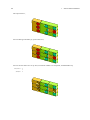
7.15.1 box definition . .
7.15.2 3dshow example
.
.
.
.
.
.
.
.
.
.
.
.
.
.
.
.
.
.
.
.
.
.
.
.
.
.
.
.
.
.
.
.
.
.
.
.
.
.
.
.
.
.
.
.
.
.
.
.
.
.
.
.
.
.
.
.
.
.
.
.
.
.
.
.
.
.
.
.
.
.
.
.
.
.
.
.
.
.
.
.
.
.
.
.
.
.
.
.
.
.
.
.
.
.
.
.
.
.
.
.
.
.
.
.
.
.
.
.
.
.
.
.
.
.
.
.
.
.
.
.
.
.
.
.
.
.
.
.
.
.
.
.
.
.
.
.
.
.
.
.
.
.
.
.
.
.
.
.
.
.
.
.
.
.
.
.
.
.
.
.
.
.
.
.
.
.
.
.
.
.
.
.
.
.
.
.
.
.
.
.
.
.
.
.
.
.
.
.
.
.
.
.
.
.
.
.
.
.
.
.
.
.
.
.
.
.
.
.
.
.
.
.
.
.
.
.
.
.
.
.
.
.
.
.
.
.
.
.
.
.
.
.
.
.
152
154
156
158
160
161
8
Volume and Area calculation by tally function
164
9
Processing dump file
166
10 Output cutoff data format
170
11 Supplementary explanation for region error checking
171
12 Additional explanation for the parallel computing
12.1 PHITS input file definition . . . . . . . . . . . . . . . .
12.2 maxcas, maxbch definition . . . . . . . . . . . . . . . .
12.3 Treatment of abnormal end . . . . . . . . . . . . . . . .
12.4 PHITS startup . . . . . . . . . . . . . . . . . . . . . . .
12.5 ncut, gcut, pcut and dumpall file definition in the PHITS
12.6 Read in file definition in the PHITS . . . . . . . . . . .
13 FAQ
13.1
13.2
13.3
13.4
.
.
.
.
.
.
.
.
.
.
.
.
.
.
.
.
.
.
.
.
.
.
.
.
.
.
.
.
.
.
.
.
.
.
.
.
.
.
.
.
.
.
.
.
.
.
.
.
.
.
.
.
.
.
.
.
.
.
.
.
.
.
.
.
.
.
.
.
.
.
.
.
.
.
.
.
.
.
.
.
.
.
.
.
.
.
.
.
.
.
.
.
.
.
.
.
.
.
.
.
.
.
172
172
172
172
172
172
173
Questions related to parameter setting . . . . . . . . . . . . . . . .
Questions related to error occurred in compiling or executing PHITS
Questions related to Tally . . . . . . . . . . . . . . . . . . . . . . .
Other questions . . . . . . . . . . . . . . . . . . . . . . . . . . . .
.
.
.
.
.
.
.
.
.
.
.
.
.
.
.
.
.
.
.
.
.
.
.
.
.
.
.
.
.
.
.
.
.
.
.
.
.
.
.
.
.
.
.
.
.
.
.
.
.
.
.
.
.
.
.
.
.
.
.
.
.
.
.
.
174
174
174
175
175
.
.
.
.
.
.
.
.
.
.
.
.
.
.
.
.
.
.
.
.
.
.
.
.
.
.
.
.
.
.
14 Concluding remarks
176
index
179
v
1
1
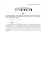
Introduction
Particle and heavy ion transport code is an essential implement in design and study of spacecrafts and accelerator facilities. We have therefore developed the multi-purpose Monte Carlo Particle and Heavy Ion Transport
code System, PH I TS ,1, 2) based on the NMTC/JAM.3) The physical processes which we should deal with in a
multipurpose simulation code can be divided into two categories, transport process and collision process. In the
transport process, PHITS can simulate a motion under external fields such as magnetic and gravity. Without the
external fields, neutral particles move along a straight trajectory with constant energy up to the next collision point.
However, charged particles and heavy ions interact many times with electrons in the material losing energy and
changing direction. PHITS treats ionization processes not as collision but as a transport process under an external
field. The average dE/dx is given by the charge density of the material and the momentum of the particle taking
into account the fluctuations of the energy loss and the angular deviation. The second category of the physical
processes is the collision with the nucleus in the material. In addition to the collision, we consider the decay of the
particle as a process in this category. The total reaction cross section, or the life time of the particle is an essential
quantity in the determination of the mean free path of the transport particle. According to the mean free path,
PH I TS chooses the next collision point using the Monte Carlo method. To generate the secondary particles of the
collision, we need the information on the final states of the collision. For neutron induced reactions in low energy
region, PHITS employs the cross sections from Evaluated Nuclear Data libraries. For high energy neutrons and
other particles, we have incorporated two models, JAM4) and JQMD5) to simulate the particle induced reactions
up to 200 GeV and the nucleus-nucleus collisions, respectively.
Recently PH I TS introduces an event generator for particle transport parts in the low energy region. Thus,
PH I TS was completely rewritten for the introduction of the event generator for neutron-induced reactions in energy
region less than 20 MeV. Furthermore, several new tallis were incorporated for estimation of the relative biological
effects. This report includes descriptions on new features and functions introduced into the code. For examples,
GG geometry, parallelization, DPA tally, neutron, photon and electron transportation, and detailed descriptions
how to setup the geometry as well. In order to keep comprehensive descriptions as the manual of PH I TS , this
report includes description on some parts of the NMTC/JAM code, which is an origin of code structure of PH I TS .
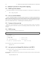
1.1 Recent technical notice
To get graphical output of 3dshow, you need AN GE L ver. 4.20 or higher version. Since PH I TS already include
AN GE L ver. 4.35, you can compile AN GE L ver. 4.35 itself from the source of PH I TS .
From ver. 1.30, we can calculate the transport of neutron and proton based on the nuclear data LA150. And we
also introduced the multiplier in track tally like FM card of MCNP. We have included a dose conversion coefficient
estimated by JAERI people.7) Then you can get directly dose values in track lenght tally.
From ver. 1.50, the coordinate transformation is available in r-z and xyz scoring meshes of tally, magnetic field
and source functions.
From ver. 1.60, you can write the information on particles on the dump file in cross, time and product tallies,
and the dump file can also be used as a source of the calculation. The magnetic field is available in non void region.
By this, you can treat collion processes in the magnetic field.
From ver. 1.70, we introduced the gravity and the spin variable of nucleon for neutron optics study coupled
with magnetic field. We have added angle straggling for heavy ions.
From ver. 1.80, we combined the JAM and JQMD code. By this JAMQMD code, you can treat high energy
heavy ion collisions up to 100 GeV/u. We introduced a function of time dependent material, by which we can treat
a moving material like chopper.
From ver. 2.00, we introduced some functions for neutronics, duct source option, super mirror, elastic option
and time dependent magnetic field. We made new tallies, LET tally and DEPOSIT tally. We created a new model
to treat low energy neutron transport by Event Generator mode.
From ver. 2.05, we added multi-source function by which one can treat multi-source particles and complicated
source regions. In addtion, we introduced a description of any analytical functions defined by users for the energy
distribution of the source particles. For angular distribution of the source particles, one can also use any analytical
functions and data.
From ver. 2.06, we made a new tally, DEPOSIT2 tally, by which one can see a correlation of the deposit energy
distribution between two regions. We also added a new section, [Timer], which can reset and stoop the time of a
particle. Combined these two functions, we can also see a correlation between TOF and the deposit energy. We
added an angle variable in PRODUCT tally. By this, you can easily calculate DDX of thin material.
1 INTRODUCTION
2
From ver. 2.08, we added the particle specification in the counter section.
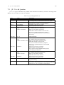
From ver. 2.15, you can use the Event Generator mode (e-mode) for thermal neutrons, and the neutron scattering with the scattering laws S (α, β) can be also treated. In the previous PH I TS , neutron spectra obtained by e-mode
in the thermal energy region were unnatural.
From ver. 2.18, we replaced the source codes for reading GG geometry and for reading/writing nuclear data
written in the ACE format by our original program. This revision does not influence results of the PH I TS calculation.
From ver. 2.24, we added the function to simulate nuclear “giant resonances” induced by photons with energies
below 20MeV.
From ver. 2.26, we added the function to transport knocked-out electrons so-called δ-rays produced along the
trajectory of a charged particle in materials as secondary particles. Setting a threshold energy parameter for each
region in the [Delta Ray] section, you can explicitly generate δ-rays above the threshold energy.
From ver. 2.28, you can use options of dumpall and dump for [t-cross], [t-time], and [t-product]
tallies also on the MPI parallel computing. PH I TS with these options makes files to the number of (PE−1) for
writing down separately each of results calculated by the (PE−1) nodes, where PE is the total number of used
Processor Elements. For reading, the treatment of the results is in the same way.
From ver. 2.30, for the calculation of DPA (Displacement Per Atom), the radiation damage model in PH I TS
has been improved using the screened Coulomb scattering. And, we added a [multiplier] section to define any
factors depending on energies of particles when a multiplier option is used in a [t-track] section.
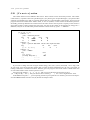
Please see read.me.phits230.engl file for the detail.
1.2 Development members
Koji Niita
RIST (Research Organization for Information Science & Technology).
Norihiro Matsuda, Shintaro Hashimoto, Yosuke Iwamoto, Tatsuhiko Sato, Hiroshi Nakashima, Yukio Sakamoto,
Tokio Fukahori, Satoshi Chiba
JAEA (Japan Atomic Energy Agency).
Hiroshi Iwase
KEK (High Energy Accelerator Research Organization).
Lembit Sihver
Chalmers University, Sweden.
The following members also contributed to the development of PH I TS .
Hiroshi Takada, Shin-ichro Meigo, Makoto Teshigawara, Fujio Maekawa, Masahide Harada and Yujiro Ikeda
JAEA (Japan Atomic Energy Agency).
Takashi Nakamura
Tohoku University.
Davide Mancusi
Chalmers University, Sweden.
3
2
Models implemented in the code
2.1 JAM model
2.1.1 Main feature of JAM
JAM (Jet AA Microscopic Transport Model8) ) is a hadronic cascade model, which explicitly treats all established hadronic states including resonances characterized by explicit spin and isospin as well as their anti-particles.
We have parametrized all hadron-hadron cross sections√ based on a resonance model and string model by fitting
available experimental data. At center of mass energy s < 4 GeV, the inelastic hadron-hadron collisions are described by resonance formations and their decays, and at higher energies, string formation and their fragmentation
into hadrons are assumed.
We have parametrized the resonance formation cross sections in terms of an extended Breit-Wigner
form and
√
used established data9) for decay probabilities to various channels. At an energy range above s = 4-5 GeV, the
(isolated) resonance picture breaks down because width of resonances
becomes wider and which their spacing
√
get closer. Hadronic interactions at an energy range 4-5 < s < 10-100 GeV is called “soft process” which
is characterized by a small transverse momentum transfer, and string phenomenological models are known to
describe the data for such soft process well. In this picture, a hadron-hadron collision leads to a longitudinal string
like excitation. In actual description of the string formation, we follow a prescription adopted in HIJING model.10)
The strings are assumed to hadronize via quark-antiquark or diquark-antidiquark creation. As for the fragmentation
of the strings, we adopted Lund fragmentation model PYTHIA6.1.11)
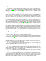
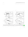
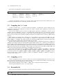
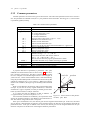
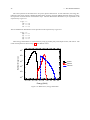
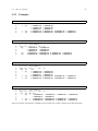
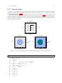
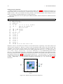
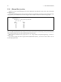
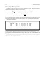
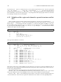
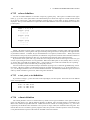
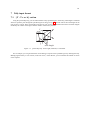
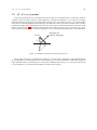
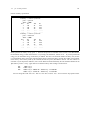
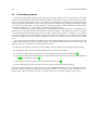
In Figure 2.1, we show a fitted total cross section with experimental data9) and inelastic components of pp
collision as a function of the c.m.
√ energy. Inelastic cross sections are assumed to be filled up by the resonance
formations (gray region) up to s = 3-4 GeV. At higher energies, the difference between experimental inelastic
cross section and sum of the resonance formation cross sections are assigned to the string formation. The following
resonance excitation channels are implemented for the nucleon-nucleon scattering in JAM:
s
Figure 2.1: Total cross section and inelastic components of pp collision as a function of the c.m. energy.
(1) NN → N∆(1232), (2) NN → NN ∗ , (3) NN → ∆(1232)∆(1232),
(4) NN → N∆∗ , (5) NN → N ∗ ∆(1232), (6) NN → ∆(1232)∆∗ ,
(7) NN → N ∗ N ∗ , (8) NN → N ∗ ∆∗ , (9) NN → ∆∗ ∆∗
4
2 MODELS IMPLEMENTED IN THE CODE
Here N ∗ and ∆∗ represent higher non-exotic baryonic states below 2 GeV/c2 . In Fig. 2.1, we also plot contributions
from the above channels (1) (dashed line), (2) (dot-dot-dashed line), (4) (long dashed line) and a sum of the other
channels (dot-dashed line) to the resonance formation cross section.
For nuclear reactions in JAM, we use a full cascade method described in the following. Each hadron has its
position and momentum and moves along a straight line until it experiences next hadron-hadron and hadron-lepton
collisions, decay or absorption. The initial position of each nucleon is sampled by a parameterized distribution of
nuclear density. Fermi momentum of nucleons is assigned according to the local Fermi momentum as a function of
the density. We do not take into account the mean field effects except for the initial nucleons. The initial nucleons
in a target nucleus stay on the initial positions until a collision with other hadrons take place. The interaction
probabilities of hadron-hadron collision are determined by the method of so-called “closest distance approach”;
if
distance for any pair of particles becomes less than an interaction range specified by
√ the√minimum relative
√
√
σ( s)/π, where σ( s) is the total cross section for the pair at the c.m. energy s, then the particles are
assumed to collide. This cascade method has been widely used to simulate high energy nucleus-nucleus collisions.
However, geometrical interpretation of the cross section violates causality and the time ordering of the collisions in
general differs from one reference-frame to the other. These problems have been studied by several authors.12, 13)
We have adopted a similar procedure as that in Ref.12) for the collision criterion to mimic the reference-frame
dependence. Pauli-blocking for the final nucleons in two-body collisions are also considered.
2.1.2 Elementary cross sections of hadron-hadron
Details of the parametrization of hadron-hadron cross sections in JAM is described in Ref.8) . Here, we demonstrate typical examples of the elementary hadron-hadron cross sections obtained by JAM and compare results with
experimental data.
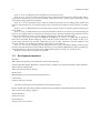
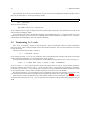
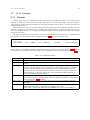
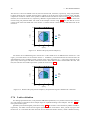
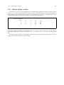
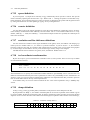
In Figure 2.2 we show calculated rapidity y and transverse momentum distributions of protons, positive and
negative pions for proton-proton collisions at 12 GeV/c incident laboratory momentum and also data from Ref.14) .
A proton stopping behavior around y ∼ 0 and pion yields are well described by JAM. Within JAM model, fast
protons come from resonance decays and mid-rapidity protons from string fragmentation.
Figure 2.2: A rapidity y distributions (left panel) and transverse momentum distributions (right panel) of proton,
π+ and π− in pp collisions at 12 GeV/c incident laboratory momentum. Histograms are results obtained with JAM,
while the squares denote experimental data are from Ref.15) .
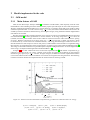
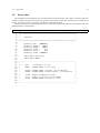
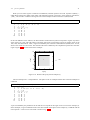
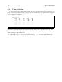
Figure 2.3 shows energy dependence of exclusive pion production cross sections in pp reactions. We compare
2.1 JAM model
5
results of the simulation with data.15) Overall agreement is achieved
in these exclusive pion productions. Smooth
√
transition from the resonance picture to the string picture at s = 3-4 GeV is realized since no irregularity of the
energy dependence appears in the calculated results.
s
s
Figure 2.3: Energy dependence of exclusive pion production cross sections for proton-proton collision as a function
of the c.m. energy. Solid lines are results obtained with JAM, while the squares denote experimental data from
Ref.15) .
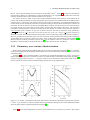
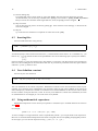
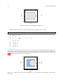
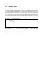
As other examples of the hadron-hadron cross sections, we plot, in Fig. 2.4, the total and elastic π− p and
K p cross sections parametrized by JAM (upper panel), and energy dependence of the exclusive cross sections of
K − p → π0 Λ and K − n → π− Σ0 (lower panel). Data are taken from Refs.9, 16) .
+
These examples indicate that the parametrization of the elementary hadron-hadron cross sections in JAM is
accurate enough for high energy particle transport calculations.
2 MODELS IMPLEMENTED IN THE CODE
6
s
s
s
Figure 2.4: Parametrization of the total and elastic π− p and K + p cross sections (upper panel), and energy dependence of exclusive cross sections of K − p → π0 Λ and K − n → π− Σ0 (lower panel). Data are taken from Refs.9, 16) .
2.2 JQMD model
7
2.2 JQMD model
JQMD (JAERI Quantum Molecular Dynamics) code17) has been widely used to analyze various aspects of
heavy ion reactions as well as of nucleon-induced reactions.18, 19) In the QMD model, a nucleus is described as a
self-binding system of nucleons, which are interacting with each other through effective interactions in a framework
of molecular dynamics. One can estimate yields of emitted light particles, fragments and of excited residual nuclei
resulting from heavy-ion collisions. The QMD simulation, JAM simulation as well, describes a dynamical stage of
nuclear reactions. At the end of the dynamical stage, we will get excited nuclei from these simulations. To get final
observables, these excited nuclei should decay in a statistical way. We have employed GEM model20) (generalized
evaporation model) for light particle evaporation and fission process of the excited residual nucleus.
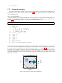
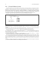
So far the QMD model has shed light on several exciting topics in heavy-ion physics, for example, multifragmentation, flow of the nuclear matter, and energetic particle productions.21) In Fig. 2.5 we show two examples
of basic observables from heavy-ion reactions calculated by JQMD code. In Fig. 2.5(a) we represent results of π−
energy spectra for the reaction 12 C+12 C at 800 MeV/u in lab. The result of JQMD code reproduces experimental
data.22) We notice that this calculation has been done in the same formulation and also with the same parameter
set as used in nucleon-induced reactions.18, 19) Next example is neutron energy spectra from the 400 MeV/u 12 C
incident reaction on 208 Pb, which is shown in Fig. 2.5(b). Neutrons produced in heavy-ion reactions is very
important in shielding design of spacecrafts and other facilities because of their large attenuation length in shielding
materials. Secondary neutrons from heavy-ion reactions have been systematically measured using thin and thick
targets at HIMAC23, 24, 25, 26, 27) facility. Fig. 2.5(b) shows that JQMD code roughly reproduces measured cross
sections for C beams with thin target.
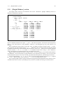
Figure 2.5: (a) (left panel) π− momentum spectra for the reaction 12 C (800MeV/u)+12 C and (b) (right panel)
neutron energy spectra for the reaction 12 C (400MeV/u)+208 Pb at different laboratory angles as indicated in the
figure. The solid histograms and the solid lines are the results of the JQMD code and the open circles and solid
squares denote the experimental data taken from22, 23) . The ordinate of left panel is the Lorentz invariant double
differential cross section as a function of the momentum of the emitted pion, while the ordinate of the right panel
is the double differential cross section as a function of the neutron energy.
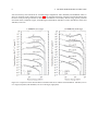
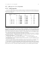
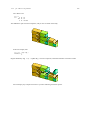
PH I TS has incorporated JQMD code for the collision part of the nucleus-nucleus reactions to describe the secondary neutron yields from the thick target. In order to investigate the accuracy of the PH I TS code in the heavy ion
transport calculation, we have first compared the results with the experimental data measured by Kurosawa et al.
The measured secondary neutrons produced from thick (stopping length) targets of C, Al, Cu, and Pb bombarded
8
2 MODELS IMPLEMENTED IN THE CODE
with various heavy ions from He to Xe. Incident energies ranged from 100 to 800 MeV/u from HIMAC. Here we
show two examples of the comparisons in Fig. 2.6. It is confirmed from these comparison with measurements that
the PH I TS code provides good results on the angular distributions of secondary neutron energy spectra produced
from thick carbon, aluminum, copper, and lead targets bombarded by 100 MeV/u carbon, 400 MeV/u carbon, and
400 MeV/u iron ions.
Figure 2.6: Comparison of the neutron fluence calculated with PH I TS and the measured data for 100 MeV/u C ion
on C target (left panel) and 400 MeV/u Fe ion on Pb target (right panel).
2.2 JQMD model
9
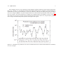
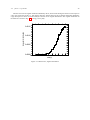
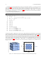
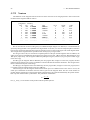
Next validation of PH I TS is the comparisons of the spallation products induced in a thick target by high energy
heavy ions. Yashima et al. systematically measured the residual radioactivities by irradiating Ar(230, 400 MeV/u),
Si(800 MeV/u), Ne(100, 230, 400 MeV/u), C(100, 230, 400 MeV/u), He(100, 230 MeV/u) and p(100, 230 MeV)
ions on a Cu target at HIMAC. They have compared the PH I TS results with the experimental results of the production cross sections. One of the results for Cu sample of Ar induced reaction at 230 MeV/u is shown in Fig. 2.7.
The results of PH I TS agree in general with the experimental values within a factor of 2, except for heavy products
close to target nuclide and the specific products in the lighter mass region.
Figure 2.7: Comparison of production cross section calculated with PH I TS and the measured data for 230 MeV/u
Ar ion on Cu target.
10
2 MODELS IMPLEMENTED IN THE CODE
2.3 New features of PHITS
2.3.1 Event generator mode for low energy neutron incident reactions
Energy and momentum are not conserved in an event of transport calculations based one-body Bolzmann
equation with the nuclear data base if there are more than 2 particles in the final state. They are conserved as an
average over many Monte Carlo events. Moreover, solutions of Boltzmann equation include only mean values of
the one-body observables in the phase space. It cannot give us two-body and higher correlations, since Bolzmann
equation and also the nuclear data base has no information for the two-body and higher correlations. A typical
example of such higher correlation is deposit energy distribution treated in [T-Heat] tally. This cannot be calculated
by one-body Bolzmann equation.
For high energy nuclear reactions, there is no enough evaluated data base. Then we employed some nuclear reaction models, such as JAM and QMD. These reaction models can describe all ejectiles of the reaction keeping the
energy and momentum by the Monte Carlo method. Therefore we can extract any information from the transport
calculation with these reaction models. In this sense, these transport codes are called as “event generators”.
In PH I TS , we have two domains, event generator for high energy and transport for low energy with the nuclear
data. Recently, even in low energy fields, the correlated quantities, such as the deposit energy distribution, are
often required, for examples, estimations of single upset error of semiconductor, biological effects and in a microdosimetry field. For these requirement, we changed the transport algorithm for low-energy neutrons from that
based on solving Boltzmann equation (in a similar manner as MCNP) to the original one based on the concept of
the event generator, and developed an “event generator mode” for all energy region in PH I TS . This mode is chosen
by “e-mode=1” in the parameter section.
The detail of this mode will be published elsewhere. Here we explain the outline of this mode. The evaluated
nuclear data base can describe the total cross section, the channel cross sections, i.e. capture, elastic, (n, n′ )
and (n, Nn′ ) cross sections, and inclusive double differential cross sections of outgoing neutrons. From these
information, energy and momentum of the residual nucleus are not determined uniquely, since information is
lacking. Therefore, we have developed a model to determine the energy and momentum of all ejectile by using
information of the data base for neutron and a special statistical decay model. At first, we use the total cross section
and channel cross sections of the data base. For each channel, we assume the following models. The excitation
energy and momentum of composite nucleus are determined uniquely from incident energy and target nucleus. We
apply a special statistical decay model in which the decay width of neutron is zero. Then we can determine all
information on ejectiles, in this case, charged particles, photon and residual nucleus. For an elastic reaction, we
determine the momentum of outgoing neutrons according to the data base. By the kinematics of this reaction, we
can uniquely determine the momentum of the residual nucleus. We apply a similar method for the capture case. In
this case we can uniquely determine the excitation energy as well as the momentum of the residual nucleus. We
then apply the statistical decay process without neutron width. Finally, for (n, Nn′ ) reaction, we apply a similar way
as in the (n, n′ ) case, but after one nucleon emission, we apply the statistical decay process with all decay channels.
In this case, number of emitted neutrons is not always coincident with a number indicated in the data base. But we
have checked this discrepancy has very small effect. By these processes, we can treat low energy neutron collisions
as an “event” which means the energy and momentum are conserved in each event. Therefore, by this mode, we
can extract any information, e.g. the kinetic energy distribution of the residual nuclei, two-particle correlation, etc.
2.3.2 Microscopic approach for estimation of relative biological effectiveness
Calculation of the probability density of deposition energies in microscopic sites, called as lineal energy y
or specific energy z, is of great importance in estimation of relative biological effectiveness (RBE) of charged
particles. However, such microscopic probability densities cannot be directly calculated by PH I TS simulation using
[T-Deposit] or [T-Heat] tallies, since PH I TS is designed to simulate particle motions in macroscopic scale, and
employs a continuous-slowing-down approximation (CSDA) for calculating the energy loss of charged particles.
We therefore introduced a special tally named [T-SED] for calculating the microscopic probability densities using
a mathematical function that can instantaneously calculate quantities around trajectories of charged particles. The
function was developed on the basis of track structure simulation, considering productions of δ-rays and Auger
electrons. Note that the name of “SED” derives from “Specific Energy Distribution”. Details of the calculation
procedure are given elsewhere.28, 29)
2.3 New features of PH I TS
11
Using this tally, we can get information on probability densities of y and z in water. We can also calculate the
probability densities in different materials, although the accuracy has not been checked yet. Similar to [T-LET], the
dose is only counted in an energy loss of charged particles and nuclei, and thus, we must use the event generator
mode (e-mode = 1) if we would like to transport low-energy neutrons. The deposition energy in microscopic sites
can be expressed by deposit energy ϵ in MeV, lineal energy y in keV/µm or specific energy z in Gy. The definitions
of these quantities are given in ICRU Report 36.30) Usage of [T-SED] is similar to that of [T-LET].
3 INSTALLATION
12
3
Installation
PH I TS is coded by the Fortran77. PH I TS can be compiled by almost Fortran77 software on various operation
systems. We have already checked operations on the DEC, SUN, HP, AIX workstations, and PC, Windows, and
Linux.
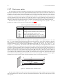
3.1 Source files and data files
The list of PH I TS source and include files is shown as followings. These files should be put together in a same
directory.
List 3.1
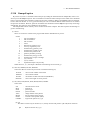
• Source file
unix.f
unix90.f
mpi-non.f
usrsors.f
usrmgf1.f
usrelst1.f
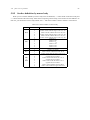
mdp-uni.f mdp-win.f
mdp-uni90.f
mpi-lin.f
anal-002.f
usrmgf3.f usrmgt1.f
usrelst2.f usrdfn1.f
analyz.f
nreac.f
read00.f
talls01.f
talls06.f
update.f
ggs00.f
geocntl.f
ggm05.f
ovly14.f
celimp.f
ovly12.f
read01.f
talls02.f
talls07.f
wrnt12.f
ggs01.f
ggm01.f
ggm06.f
ovly15.f
dataup.f
ovly13.f
read02.f
talls03.f
tallsm1.f
wrnt13.f
ggs02.f
ggm02.f
ggm07.f
getflt.f
partrs.f
sors.f
talls04.f
tallsm2.f
read03.f
ggs03.f
ggm03.f
ggm08.f
magtrs.f
range.f
talls00.f
talls05.f
tallsm3.f
marscg.f
wrnt10.f
ggm04.f
a-angel.f
main.f
sdml.f
jbook.f
fismul.f
dklos.f
gem.f
masdis.f
ncasc.f
gemset.f
atima01.f
nelst.f
utl01.f
atima02.f
nevap.f
utl02.f
atima03.f
bert.f
utlnmtc.f
isobert.f
mars00.f
bertin.f
gamlib.f
isodat.f
mars01.f
bert-bl0.f
erupin.f
randmc.f
mars02.f
bert-bl1.f
erup.f
energy.f
mars03.f
bert-bl2.f
fissn.f
ndata01.f
mars04.f
jamin.f
jam.f
jamcross.f jampdf.f
jambuu.f
jamana.f
jamdat.f
jamsoft.f
pyjet.f
jamcoll.f
jamhij.f
pythia.f
jamdec.f
jamhard.f
pysigh.f
qmd00.f
qmdmfld.f
qmdcoll.f
qmddflt.f
qmdgrnd.f
qmdinit.f
utl03.f
a-main0.f
a-func.f
a-main1.f
a-utl00.f
a-hsect.f
a-line.f
a-wtext.f
usrmgt2.f
usrdfn2.f
Only mdp-uni.f, mdp-uni90.f and mdp-win.f are OS dependent files in the above list. You have to specify,
which file you use, in a makefile. mdp-uni.f and mdp-uni90.f should be used on the UNIX system, and
mdp-win.f on the Windows system. mdp-uni90.f is prepared for fortran 90 compilers. These mdp-uni.f and
mdp-win.f files are used in order to obtain a DATE, TIME, and CPU times in the code. The mpi-non.f and
mpi-lin.f are prepared for the non-parallel and the MPI parallel computation.
3.2 Compiling the PH I TS code
13
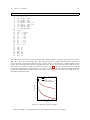
PH I TS needs 14 include files as shown in followings
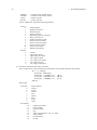
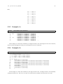
List 3.2
• Include files
bert.inc
param.inc
ggmparam.inc
atimacnt.inc
gamlib.inc
param00.inc
mmbank.inc
atimadim.inc
jam1.inc
param01.inc
angel00.inc
atimasys.inc
jam2.inc
param02.inc
angel01.inc
jam3.inc
ggsparam.inc
A data file trxcrd.dat is necessary if you set the option of the photon emission from residual nuclei. You
must put the trxcrd.dat file into a directory specified in your input.
3.2 Compiling the PHITS code
In order to compile PH I TS , you need to modify the makefile. Uncomment the options suitable for your
environment. Then you can compile PH I TS code by the “make” command. Short explanations of terms in the
makefile are written below.
If you want to compile the PH I TS code for the MPI parallel computing, set OBJPARA = mpi-lin.o in the
makefile, otherwise, OBJPARA = mpi-non.o. The MPI parallel computing for PH I TS was checked its operation
on a PC cluster system by the Linux pgf77. On other cluster systems the parallel computing is not supported yet,
however it may be built on the systems if the MPI is installed, since the mpi-lin.f is written by MPI common
functions.
OBJ1 includes user definition files. usrsors.f is a user definition source routine, anal-002.f is a user
definition nuclear reaction analysis routine, usrmg1.f, usrmg3.f are sample programs for neutron magnetic
fields, usrdfn1.f, usrdfn2.f are sample routines for [t-deposit] and mdp-uni.f is a routine to obtain elapse
time for UNIX system. Modify these options depending on your needs.
Routines listed in OBJ2 include the param.inc. Some important arrays are defined in the param.inc. usrmgt1.f,
usrmgt2.f are sample routines for time dependent magnetic fields, usrelst1.f, usrelst2.f are sample routines for elastic angular distribution of low energy neutrons. In the case that param.inc is modified, only routines
listed in OBJ2 are re-compiled automatically by the make command. It is noted that the other include files are not
linked with related routines in this makefile. OBJ3 contains new routines such as the GEM. In OBJ4, OBJ5, and
OBJ6, correspond to old routines, JAM routines, and QMD routines respectively.
Source files related with the GG are read03.f, ggs00.f, ggs01.f, ggs02.f, and ggs03.f. Source files
related with the CG are marscg.f, mars00.f, mars01.f, mars02.f, mars03.f, and mars04.f. Source files
for neutron transport part are ggm01.f, ggm02.f, ggm03.f, ggm04.f, ggm05.f, ggm06.f, and ggm07.f. Source
files for AN GE L part are a-angel.f, utl03.f, a-func.f, a-utl00.f, a-main0.f, a-main1.f, a-hsect.f,
a-line.f, and a-wtext.f.
3.3 Compiling ANGEL
AN GE L is included in the PH I TS sources, in other word, AN GE L is installed automatically in the PH I TS code.
But you will need a stand-alone AN GE L for off line plotting. You can compile the stand-alone AN GE L easily using
the “make.ang” file, which included in the PH I TS source files.
After modify the make.ang, execute “make -f make.ang” to compile the stand-alone AN GE L .
Concerning about details for AN GE L , see AN GE L manual.
3.4 Executable file
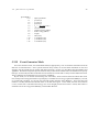
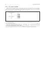
PH I TS code can be executed on the UNIX system by the following command,
List 3.3
• command line to execute PH ITS
phits100 < input.dat > output.dat
3 INSTALLATION
14
This command can not be used on the Windows system. You can use instead another method. Prepare a file (in
this case, let name phits.in ) written by following format.
List 3.4
• the first line of the standard input
file = input.file
Then you can run PH I TS by
phits100 < phits.in > output.dat
By the command, PH I TS open the input.file and read the input information. This method can be used on the
other systems including the UNIX.
If you run the PH I TS code by the parallel computing, the method shown in List 3.3 can not be used even on the
UNIX system. Instead you can use the List 3.4 method on the parallel calculation. In addition, PH I TS is forced to
read the input file named phits.in on the parallel computing.
3.5 Terminating PHITS code
Once PH I TS is executed, it creates the batch.now file. The batch.now file contains an elapse information
after every batch. It also contains each PE status on the parallel calculation. You can check if PE abort is occurred
by the batch.now.
The first line of the batch.now is written as
1 <--- 1:continue, 0:stop
If you change the value “1” into “0”, the calculation will be terminated and the summary and results are provided
for the events until terminated. It is an useful function shown in below.
Associated with the batch.now, a new parameter was included by the parameter section. You can specify it as
itall = 2
# (D=0) 0:no tally at batch, 1:same, 2:different
If you set itall = 1, PH I TS outputs the latest results (tally output) after every batch. On the parallel calculation,
results are created by every batch × ( PE −1 ). In the case of itall = 1, the results are overwritten in same files.
On the other case of itall = 2, the results after every batch are written in different named file. Results are named
by user specified name + batch number. The final results are written in the user specified file.
By using this functions, you can terminate a PH I TS calculation at any time with checking a latest result. Also
you can monitor the latest results with graphical plot automatically made by PH I TS (See section 6.7.15).
rijk written in the batch.now file is the initial random number of the current batch. For example, in cases
of unsuccessful termination of PH I TS , you can reproduce the calculation of the specified batch using the value of
rijk.
3.6 Array sizes
15
3.6 Array sizes
You should check and modify the array sizes described in the param.inc file. The “mdas” is the most important
variable. It specifies the total size of arrays for geometry, tally output, nuclear data, and bank. You can find out the
current use in a input echo (corresponds “ output.dat” in previous example).
The bank size can be set in the parameter section. If the bank becomes full, odd arrays in mdas are used. The
default param.inc is shown below.
List 3.5
1:
2:
3:
4:
5:
6:
7:
8:
9:
10:
11:
12:
13:
14:
15:
16:
17:
18:
19:
20:
21:
22:
23:
24:
25:
26:
27:
28:
29:
• param.inc
************************************************************************
*
*
*
’param.inc’
*
*
*
************************************************************************
parameter
parameter
parameter
parameter
parameter
parameter
(
(
(
(
(
(
mdas
kvlmax
kvmmax
itlmax
inevt
latmax
=20000000
=
3000
=
10000
=
40
=
70
= 2000000
)
)
)
)
)
)
common /mdasa/ das( mdas )
common /mdasb/ mmmax
*----------------------------------------------------------------------*
*
*
*
mdas
: total memory * 8 = byte
*
*
mmmax : maximum number of total array
*
*
*
*
kvlmax : maximum number of regions, cell and material
*
*
kvmmax : maximum number of id for regions, cel and material
*
*
*
*
itlmax : number of maximum tally entry
*
*
inevt : number of collision type for summary
*
*
latmax : maximum number of lattice in a cell
*
*
*
*----------------------------------------------------------------------*
4 INPUT FILE
16
4
Input File
PH I TS input consists of some sections as listed in Table 4.1 and 4.2. Each sections begins from a [Section
Name]. You can put maximum 4 blanks between the line head and the declaration of [Section Name], otherwise
(more than 4 blanks) [Section Name] is not recognized as a beginning of a section and the following part is
regarded as items of the previous section.
4.1 Sections
Table 4.1 and 4.2 shows the various sections used in PH I TS .
Table 4.1: Sections(1)
name
[title]
[parameters]
[source]
[material]
[body]
[region]
[surface]
[cell]
[transform]
[importance]
[weight window]
[volume]
[temperature]
[brems bias]
[photon weight]
[forced collisions]
[magnetic field]
[counter]
[reg name]
[mat name color]
[mat time change]
[super mirror]
[elastic option]
[timer]
[Delta Ray]
[multiplier]
description
Title
Various type of parameters
Source definition
Material definition
CG body definition
Region definition by CG
Surface definition by GG
Cell definition by GG
Definition the coordinate transform of GG surface
Region importance definition
Weight window definition
Region volume definition
Cell temperature definition
Bremsstrahlung bias definition
Photon product weight definition
Forced collision definition
Magnetic field definition
Counter definition
Region name definition for graphical plot
Material name and color definition for graphical plot
time dependent material definition
super mirror definition
elastic option definition
timer definition
production of δ-rays
multiplier definition
4.2 Reading control
17
Table 4.2: Sections(2)
name
[t-track]
[t-cross]
[t-yield]
[t-heat]
[t-time]
[t-star]
[t-dpa]
[t-product]
[t-gshow]
[t-rshow]
[t-3dshow]
[t-let]
[t-deposit]
[t-deposit2]
[t-sed]
[end]
description
Track length tally definition
Surface crossing tally definition
Residual nuclei yield tally definition
Heat developing tally definition
Time tally definition
Star density tally definition
DPA tally definition
Fragments tally definition
Region surface display definition for graphical plot
Physical quantity region display definition for graphical plot
3D graphical geometry plot definition
LET tally definition
DEPOSIT tally definition
DEPOSIT2 tally definition
SED tally definition
End of input file
It is noted that PH I TS does not read any input informations which are written below the [end] section.
4.2 Reading control
(1) Uppercase, lowercase, blank
Discrimination between lowercase and uppercase characters is not performed in the PH I TS input except for
file names. Blanks at line head and end are taken no account except for the declaration of the [Section
Name] as described before.
(2) Tab
A tab is replaced into 8 blanks.
(3) Line Connecting
If you add “ \ ” at line end, the next line is considered to be a continuation line. You can use multiple lines
to write input data by the “ \ ” connecting.
But you don’t need to use the “ \ ” connecting in the def of [body] and the def of [region]. In these
area, line is connected automatically without any symbol. This function can be also used in the [cell] and
[surface] sections but in these case, more than 4 blanks are required at the line head of connected line.
Details of this function are explained later.
(4) Line dividing
Short lines can be displayed in a line by dividing “ ; ” as
idbg = 0 ; ibod = 1 ; naz = 0
But this function is not available where the format is defined such as in the mesh description.
(5) Comment marks
You can use the following comment marks “#”, “%”, “!”, “$”. The comment out is effective from the
comment mark to the line end. You can also use “c” as a comment mark if you put “c” in the first 5 column
at line head with blanks as “c ”. In the [cell] and [surface] sections, “#” is used for cell definitions, so
only “$” is available as the comment mark in these [cell] and [surface] sections.
(6) Blank lines
Blank lines, and lines which begins from a comment mark are skipped.
4 INPUT FILE
18
(7) Section reading skip
If you add “off” after a section name as “[Section Name] off” the section is skipped (is not read).
As described later, you can write any comments after “[body]” section name as “[body] HIMAC experiment”
But you can not use comments which begins off here, if not, the [body] section is skipped.
(8) Skip in sections
You can skip from any place in sections by putting qp: at the line head. Lines from qp: to the end of the
section are skipped.
(9) Skip all
q: can be used as a terminator of a input file. It works same as the [end].
4.3 Inserting files
You can include other files in any place by
{ f ile.name } [ n1 − n2 ]
infl:
You should specify a name of a file to be inserted in { }, and the number of lines from n1 to n2 of that file in [ ]. If
there is no [ ], PH I TS includes all lines of the specified file. You can use following style to specify line numbers,
[ n1 − ],
[ −n2 ].
From line number n1 to the end, and from top to line number n2 respectively. The file insertion can be nested more
than once. The including file can be nested more than once. If you write any comments in the line, square-bracket
characters “[” and “]” cannot be used.
4.4 User definition constant
You can set your own constant as
set:
c1[ 52.3 ] c2[ 2 * pi ] c3[ c1 * 1.e-8 ]
This “set” definition can be written in anywhere. Defined user-constants can be used as numerical values in your
input file. User-constants can be re-defined any time, and these values are kept until re-defined. In the 3rd case of
above example (c3), another user-constant c1 is called in a user-constant definition. In the case, the value in which
the user-constant c1 keeps at that time, is used. So even if you re-define the c1 below the c3 definition, the value
of c3 defined here is not changed. pi is set to the value of π by default.
4.5 Using mathematical expressions
Mathematical expressions can be used in your input file. It is Fortran style. Available functions are shown in
Table 4.3.
For example,
param = c1 * 3.5 * sin( 55 * pi / 180 )
As above example as a single numerical value is expected after param =, you can put blanks in the expressions.
However it is not allowed that multiple numerical values are aligned, such as in the [body] and [region] sections.
In such region, you can close the expressions using { }, like { c1 * 2 / pi }.
4.6 Using the CG or GG
19
Table 4.3: Intrinsic Function.
FLOAT
MOD
COS
INT
NINT
COSH
ABS
SIGN
SIN
Intrinsic
EXP
SQRT
SINH
Function
LOG
ACOS
TAN
LOG10
ASIN
TANH
MAX
ATAN
MIN
ATAN2
4.6 Using the CG or GG
You have to choose between the CG system and the GG system in order to describe a geometry of calculation.
When you choose the CG, you must use the [region] and [body] sections. Or GG, you must use the [cell],
[surface], and [transform] sections.
You can not call both CG and GG systems at the same time. You can use the section-off feature as “[region]
off”, if CG and GG descriptions exist together in a input file.
4.7 Particle identification
Available particles in PH I TS are identified as in Table ??. These particles can be specified by the symbol or the
kf-code. The particles which is not specified the symbol in Table ??, are specified by only kf-code.
The other particles identified as type 11 can be defined by the kf-code as shown in followings, and these
decay-channels and life-times are also shown in below.
By adopting the QMD code, nucleus can be treated in PH I TS . The writing form of nuclide is as 208Pb, 56Fe.
The writing style Pb, Fe, etc., means all isotopes (This can not be used as projectile). Nucleus can be described by
kf=Z * 1000000 + A for the kf-code.
In the previous version of PH I TS , the photon was called “gamma” but it is called “photon” in the newer version.
Table 4.4: List of the transport particles.
ityp
1
2
3
4
5
6
7
8
9
10
11
12
13
14
15
16
17
18
19
20
symbol
proton
neutron
pion+
pion0
pion−
muon+
muon−
kaon+
kaon0
kaon−
other
electron
positron
photon
deuteron
triton
3he
alpha
nucleus
all
kf-code
2212
2112
211
111
−211
−13
13
321
311
−321
below
11
−11
22
1000002
1000003
2000003
2000004
Z*1000000+A
−
particle name
proton
neutron
π+
π0
π−
µ+
µ−
K+
K0
K−
other particle
e−
e+
γ
deuteron
triton
3
He
α
nucleus
all particles
ityp
11
11
11
11
11
11
11
11
11
11
11
11
11
11
symbol
−
−
−
−
−
−
−
−
−
−
−
−
−
−
kf-code
+ − 12
+ − 14
−2212
−2112
−311
+ − 221
331
+ − 3122
+ − 3222
+ − 3212
+ − 3112
+ − 3322
+ − 3312
+ − 3334
particle name
νe νe
νµ νµ
p
n
K0
ηη
η′
0 0
Λ Λ
Σ+ Σ+
Σ0 Σ0
Σ− Σ−
Ξ0 Ξ0
Ξ− Ξ−
Ω− Ω−
4 INPUT FILE
20
Table 4.5: Decay channel and life time
π
π+
π−
µ+
µ−
K0
0
K+
K−
η
η′
Λ0
Σ+
Σ0
Σ−
Ξ0
Ξ−
Ω−
→
→
→
→
→
→
→
→
→
→
→
→
→
→
→
→
→
→
→
→
→
→
→
→
→
→
→
→
→
→
→
γ
µ+
µ−
e+
e−
π+
π0
γ
µ+
π+
µ−
π+
γ
π0
π+
π+
π+
π0
π+
γ
p
n
p
n
Λ0
n
Λ0
Λ0
Λ0
Ξ0
Ξ−
+
+
+
+
+
+
+
+
+
+
+
+
+
+
+
+
+
+
+
+
+
+
+
+
+
+
+
+
+
+
+
γ
νµ
νµ
νe
νe
π−
π0
γ
νµ
π−
νµ
π−
γ
π0
π−
π−
π−
π0
π−
γ
π−
π0
π0
π+
γ
π−
π0
π−
K−
π−
π0
+
+
+
+
+
+
+
+
νµ
νµ
π0
π0
γ
η
η
γ
blanking fraction
100%
100%
100%
100%
100%
68.61%
31.39%
other
63.51%
other
63.51%
other
38.9%
31.9%
23.7%
other
44.1%
20.5%
30.1%
other
64.1%
other
51.57%
other
100%
100%
100%
100%
67.8%
23.6%
other
life time (sec)
0
2.6029e−8
2.6029e−8
2.19703e−6
2.19703e−6
8.922e−11
1.2371e−8
1.2371e−8
0
0
2.631e−10
7.99e−11
0
1.479e−10
2.90e−10
1.639e−10
8.22e−11
21
5
Sections format
5.1 [ T i t l e ] section
In the section, you can define a title of your calculation. Any numbers of title lines are allowed. Blank lines
are skipped in this section.
[ T i t l e ]
This is a test calculation of PHITS.
Any number of title lines are allowed.
..........
5.2 [ P a r a m e t e r s ] section
The various parameters of PH I TS can be defined in this section. The format is as below.
[ P a r a m e t e r s ]
para1 = number | file.name
para2 = number | file.name
..........
You can change the order of parameters. Each parameter has the default value. So undefined parameters use
the default values.
Parameters and default values are shown in followings. (D= ) means the default value.
5 SECTIONS FORMAT
22
5.2.1 Calculation mode
Table 5.1: parameter 1
parameter
icntl
value
(D=0)
= 0
= 1
= 2
= 3
= 4
= 5
=
=
=
=
=
=
=
6
7
8
9
10
11
12
explanation
basic control option
normal PH I TS calculation
nuclear reaction calculation, (under development)
output a CGVIEW input file
output only input echo for checking memory usage, and library, and file links
output a MARS-PF input file
no reaction, no ionization. all regions are made be void for geometry check,
and volume and area calculations
source check, source particles can be tallied by [t-product]
execute [t-gshow] tally (graphical output)
geometry output of xyz mesh tally with gshow option (graphical output)
execute [t-rshow] tally (graphical output)
geometry output of reg mesh tally with rshow option (graphical output)
execute [t-3dshow] tally (graphical output)
re-calculate from dumpall file, dumpall file is specified by file(15)
The function of nuclear reaction calculation specified as icntl=1 is under development.
By setting icntl=12, PH I TS re-calculates whole transport by reading the information from dumpall file, which
is created by dumpall=1 option. The re-calculation can describe whole transport events which were calculated
before. One needs the same input file as used in the previous calculation. maxcas and maxbch cannot be changed,
but are read from the file. It is very powerful when you want to calculate different tallies which are not used in the
previous calculation. However, please be careful that the calculation with dumpall=1 may create huge dumpall
file. This option is only available for GG geometry.
5.2.2 Number of history and Bank
Table 5.2: parameter 2
parameter
irskip
value
(D=0)
irskip>0
irskip<0
rseed
maxcas
maxbch
maxbnk
(D=0.0)
rseed<0
rseed=0
rseed>0
(D=10)
(D=10)
(D=10000)
explanation
random number control
begin calculation after skipping events
by number of irskip (for debug)
begin calculation after skipping random numbers
by number of irskip (for manual parallel computing)
initial random number option
get a initial random number from starting time.
6647299061401 (default)
use rseed as initial seed of random number
number of event per 1 batch
number of batch
size of bank array
In the PH I TS parallel calculation, number of batch should be an integer multiple of (all number of PE −1). If
not, PH I TS converts automatically the batch number as it becomes an integer multiple and as the total number of
event becomes almost same with given events. In this case, some comments are output at the end of an input echo.
5.2 [ P a r a m e t e r s ] section
23
5.2.3 Cut off energy and switching energy
Table 5.3: parameter 3
parameter
emin(1)
emin(2)
emin(i)
esmin
esmax
cmin(i)
value
(D=1.0)
(D=1.0)
(D=1.0)
i = 3-10
(D=2.0)
(D=1.e+9)
i = 12-19
i = 15-19
(D=0.001)
(D=300000)
(D=emin(i))
dmax(i)
ejamnu
i = 15-19
(D=emin(i))
(D=3500.)
ejampi
(D=2500.)
eisobar
(D=0.0)
eqmdnu
(D=3500.)
eqmdmin
ejamqmd
(D=10.0)
(D=3500.0)
emin(11)
emin(i)
explanation
proton cut off energy (MeV)
neutron cut off energy (MeV)
cut off energy for i-th particle (MeV)
(i; particle id, see Table ??)
cut off energy for others (MeV)
cut off energy for i-th particle (MeV)
(i; particle id, see Table ??)
energy unit is [MeV/nucleon]
minimum energy for range calculation for the charge particles (MeV)
maximum energy for range calculation for the charge particles (MeV)
nuclear reaction cut off energy for i-th particle (MeV)
any nuclear reactions under cmin(i) are not treated
for these nucleus, energy unit is [MeV/nucleon]
maximum energy of library use for i-th particle
switching energy of nucleon nucleus reaction calculation
from Bertini (or QMD) to JAM model (MeV)
switching energy of pion nucleus reaction calculation
from Bertini to JAM model (MeV)
maximum energy (MeV) of isobar calculation
when isobar is defined (isobar=1)
switching energy of nucleon nucleus reaction calculation
from Bertini to QMD model (MeV)
minimum energy of QMD calculation [MeV/nucleon]
switching energy from JQMD to JAMQMD [MeV/nucleon]
PH I TS uses libraries in the energy region emin < energy < dmax. If you set emin ≥ dmax, any libraries are
not used. The maximum energies for proton, neutron, photon, and electron are 150 MeV, 150 MeV, 100GeV, and
1000 MeV respectively in this version.
We create the range table of charge particles in esmin < energy < esmax. If you want to use much larger
energy, you should set esmax.
Below eqmdmin, we do not consider the nuclear reactions of d, t, α, and nucleus. Since the applicability of
QMD is restricted in low energy region and the range of nucleus is very short in the normal material, one do not
need consider the low energy reactions of nucleus for usual case. High energy heavy ion collisions are treated
by JAMQMD above 3.5GeV/u in default. This switching energy can be changed by e jamqmd. Even for nucleon
induced collisions, you can calculate the collisions by JAMQMD by changing eqmdnu, e jamnu and e jamqmd.
5 SECTIONS FORMAT
24
5.2.4 Cut off time, cut off weight, and weight window
Table 5.4: parameter 4
parameter
tmax(i)
wc1(i)
wc2(i)
swtm(i)
wupn
value
(D=1.e+9)
i = 1-20
(D=-0.5)
(D=wc1/2)
(D=1.0)
(D=5)
wsurvn
(0.6*wupn)
mxspln
(D=5)
mwhere
(D=0)
explanation
cut off time for i-th particle (nsec)
(i; particle id, see Table ??)
minimum weight for i-th particle
cutoff weight for i-th particle
minimum source weight for i-th particle
maximum value of weight window
= minimum value in [Weight Window] section × wupn
wupn ≥ 2
survival weight value
1 < wsurvn < wupn
maximum number of split, maximum multiple number of survival
mxspln > 1
where the weight window takes place
-1: at nuclear reaction, 0:both, 1: at region crossing
Cut off time should be specified as tmax(i)= [nsec] for each particle. After elapsing the cut off time, the
particle is killed. It is not effective to results for high energy particle transport, but it is useful for low energy
particle transport calculation.
Weight of a particle is changed by the importance, forced collisions, implicit captures, and weight window
functions. When the weight takes lower value than user-defined weight cut off, the particle is judged if it is killed
or not by the Russian roulette method. This function is not available for particles defined in the weight window.
In the Russian roulette method, when the weight WGT is lower than the product of WC2 and ratio R of two
importances between at source point and at current point, WC2 × R (i.e., when WGT < WC2 × R), the particle
survives with a probability, WGT/(WC1×R), which is a function of own weight WGT . Then the weight is changed
as WGT = WC1 × R. Unless, the particle is killed. If the WC1 and WC2 are given as negative, |WC1| × S WT M
and |WC2| × S WT M are set as WC1 and WC2.
If there are any particles and regions which are not set importance, these importances are set as 1
5.2 [ P a r a m e t e r s ] section
25
5.2.5 Model option (1)
Table 5.5: parameter 5
parameter
ielas
ielms
inmed
nevap
igamma
isobar
ipreeq
ieleh
ipngdr
value
(D=2)
= 0
= 1
= 2
(D=100)
(D=1)
= 0
= 1
= 2
(D=3)
= 0
= 1
= 2
= 3
(D=0)
= 0
= 1
(D=0)
= 0
= 1
(D=0)
= 0
= 1
(D=0)
= 0
= 1
(D=0)
= 0
= 1
explanation
elastic scattering option
exclude elastic scatter
include neutron elastic scatter
include neutron and proton elastic scatter
number of angle group for elastic scattering
nucleon-nucleon cross section options for Bertini model
free (nmtclb25.dat)
Cugnon old (nmtclb95.dat)
Cugnon new (nmtclb30.dat)
options for Evaporation model
without evaporation model
using DRES model
using SDM model
using GEM model
γ decay option for residual nuclei
without γ decay
with γ decay; file(14) is required. file(14)=trxcrd.dat
options for isobar model
without isobar
with isobar
options for pre-equilibrium model (when nevap=1)
without pre-equilibrium model
with pre-equilibrium model
options for electron and positron transport
no slowing down, no reaction, in the energy region above dmax(12)
make e=dmax(12), and weight=e/dmax(12)
in the energy region above dmax(12)
Options for nuclear“ giant resonances ”by photons
Without the nuclear“ giant resonance ”
With the nuclear“ giant resonance ”(In this case, file(19)
including the cross section data is required.)
It is noted that inmed=1 is the default value.
5 SECTIONS FORMAT
26
5.2.6 Model option (2)
Table 5.6: parameter 6
parameter
level
npidk
imagnf
andit
gravx
gravy
gravz
icrhi
value
(D=3)
= 1
= 2
= 3
(D=0)
= 0
= 1
(D=0)
= 0
= 1
(D=0)
= 0
= 1
= 2
(D=0)
(D=0)
(D=0)
(D=1)
= 0
= 1
explanation
level density option when nevap=1
8/A
with Baba’s parameters
with Igunatyuk’s parameters
treatment of minus charged decay particles below cut off energy
make absorbed by force
make decayed
Magnetic field
without Magnetic field
with Magnetic field
∆ angular distribution for Bertini
50% isotropic, 50% forward
all isotropic
all forward
x-component of gravity direction
y-component of gravity direction
z-component of gravity direction
option for total cross section for Nucleus-Nucleus collision
Shen formula
NASA formula
If a particle, which has decay channel, takes lower energy than cut off, the particle decays completely. In such
decay particles, minus charged particles with nspred = 0, are forced to take reaction for the purpose of forced
absorption. If it is not absorbed, then the particle is made decayed.
gravx, gravy, gravz represent directions of gravity. The gravity force acts on neutrons below 1 eV. For an
example, for gravx=1, gravy=0, gravz=0 case, the direction of the gravity is negative direction of x-axis.
5.2 [ P a r a m e t e r s ] section
27
5.2.7 Model option (3)
Table 5.7: parameter 7
parameter
ndedx
ih2o
nspred
nedisp
e-mode
usrmgt
usrelst
value
(D=2)
= 0
= 1
= 2
(D=-1)
< 0
> 0
(D=0)
= 0
= 1
= 2
= 3
= 10
(D=0)
= 0
= 1
= 10
(D=0)
= 0
= 1
(D=1)
= 1
= 2
(D=1)
= 1
= 2
explanation
option for dE/dx of charged particle and nucleus
SPAR for nucleus, NMTC for the others
ATIMA for nucleus and proton, NMTC for the others
SPAR for nucleus, proton, pion, and muon, NMTC for the others
Water (only for H2O) Ionization Potential option for ATIMA
default, 75 eV
Ionization Potential for water(eV)
option for Coulomb diffusion (angle straggling)
without Coulomb diffusion
with original Coulomb diffusion
with Moliere First Coulomb diffusion
with Moliere Third Coulomb diffusion
with Coulomb diffusion for ATIMA
energy straggling option for charged particle and nucleus
without energy straggling
with Landau Vavilov energy straggling
with energy straggling for ATIMA
option for event generator mode
normal mode
event generator mode, file(14) = trxcrd.dat is required
option for user subroutine of time dependent magnetic field
usrmgt1.f is used, which includes Wobbler magnet.
usrmgt2.f is used, which includes Pulse magnet.
option for [elastic option]
usrelst1.f is used, which is for Bragg scattering
usrelst2.f is used, which is a sample program
It should be noted that the default option for ndedx was ndedx=0 before PH I TS ver.2.00.
The option for ATIMA is under development, and it takes very long cpu time to calculate.
5 SECTIONS FORMAT
28
5.2.8 Output options (1)
Table 5.8: parameter 8
parameter
incut
igcut
ipcut
inpara
igpara
ippara
value
(D=0)
= 0
= 1
= 2
(D=0)
= 0
= 1
= 2
= 3
(D=0)
= 0
= 1
= 2
(D=0)
= 0
= 1
= 3
(D=0)
= 0
= 1
= 3
(D=0)
= 0
= 1
= 3
/wk/uname/
explanation
neutron output options below cut off
no output
output in the ncut file specified as file(12)
output in file(12) with time information
γ-ray and electron output options below cut off
no output
output γ-ray data in the gcut file specified as file(13)
output γ-ray in file(13) with time information
output γ-ray, electron, and positron data in file(13)
proton output options below cut off
no output
output in the pcut file specified as file(10)
output in file(10) with time information
ncut file name options in the parallel calculation
/wk/uname/file-name of file(12)
/wk/uname/file-name of file(12)+(PE number)
file-name of file(12)+(PE number)
gcut file name options in the parallel calculation
/wk/uname/file-name of file(13)
/wk/uname/file-name of file(13)+(PE number)
file-name of file(13)+(PE number)
pcut file name options
/wk/uname/file-name of file(10)
/wk/uname/file-name of file(10)+(PE number)
file-name of file(10)+(PE number)
/wk/ is the default directory name
uname is a user-name read in from environment variable LOGNAME
It is noted that the default of incut and igcut were changed to be 0.
In the parallel computing, files corresponding to each PE (Processor Element) are created for writing the output.
If you set inpara, igpara, or ippara=0 or 1, a file is made in the directory named by /wk/uname/ on each of
the nodes. If you set inpara, igpara, or ippara=1 or 3, the each PE number is put at the end of the filename.
The each PE writes down its result on only the corresponding file.
5.2 [ P a r a m e t e r s ] section
29
5.2.9 Output option (2)
Table 5.9: parameter 9
parameter
itall
value
(D=0)
= 0
= 1
= 2
itstep
(D=0)
= 0
= 1
(D=0)
= 0
= 1
= 2
(D=0)
= 0
= 1
(D=0)
= 0
= 1
(D=1)
= 0
= 1
imout
jmout
kmout
matadd
explanation
options for tally output after every batch
no output
in same file
in different files
file name = specified file name + batch number
option for timing of tally for changing momentum, like magnetic field
tally at reaction or surface cross (normal)
tally at each step of the transport
option of material representation in [material] section
like, mat[12], 208Pb.33c
like, mat[12], Pb-208.33c
like, m12, 82208.33c (MCNP type)
option of material density representation in [material] section
no conversion
converting particle density
option of nuclear data information
no display
writing in input echo
treatment of different densities in same material in GG
same material number
using new material number
Normally, the tallies are called at the reaction point or at the surface crossing. Thus the particle track in the
magnetic field, for an example, is shown as a straight line between collisions or between one collision and surface
crossing. If you specify itstep = 1, the trajectory is described correctly as a curve. The maximum step for the
magnetic field is set by deltm.
5 SECTIONS FORMAT
30
5.2.10 Output option (3)
Table 5.10: parameter 10
parameter
iggcm
ivout
ipout
icput
ipara
nwsors
value
(D=0)
= 0
= 1
(D=0)
= 0
= 1
(D=1)
(D=0 for GG)
= 0
= 1
(D=0)
= 0
= 1
(D=0)
= 0
= 1
(D=0)
explanation
option of GG warnings
no echo
in input echo
volume display options in the input echo
in [volume] section
in [region] section
importance display options in the input echo
in [importance] section
in [region] section
this function is only available when all particles
are set for the same importance value
CPU time count options
without count
with count
parameter display options
only described parameters
all parameters
write down the information on nwsors source particles on file(6)
CPU time counting is not available by default, for saving calculation time. If you want to know CPU time for
each process, set icput=1.
If you set ipara=1, you can confirm all parameters in the PH I TS code.
5.2 [ P a r a m e t e r s ] section
31
5.2.11 Output option (4)
Table 5.11: parameter 11
parameter
ivoxel
dumpall
idpara
value
(D=0)
=0
=1
=2
(D=0)
= 0
= 1
= -1
(D=3)
= 0
= 1
= 3
/wk/uname/
explanation
read and write voxel data in binary
not using file(18)
read from voxel data in binary file(18)
write down voxel data in binary on file(18)
dumpall option
no dump
write down all information on file(15) as binary data
write down all information on file(15) as ASCII data
dumpall file name option in the parallel calculation
/wk/uname/file-name of file(15)
/wk/uname/file-name of file(15)+(PE number)
file-name of file(15)+(PE number)
/wk/ is the default directory name
uname is a user-name read in from environment variable LOGNAME
For time shortening, you can use ivoxel parameter. When you perform PH I TS calculation with ivoxel=2,
voxel data are output in file(18) in binary. From the next calculation with ivoxel=1, a process of the data
output is omitted and the calculation time is shortened.
By icntl=12, PH I TS re-calculates whole transport by reading the information from dumpall file, which is created if you use the dumpall option. The re-calculation can describe whole transport events which were calculated
before. One needs the same input file as used in the previous calculation. maxcas and maxbch cannot be changed,
but are read from the file. It is very powerful when you want to calculate different tallies which are not used in
the previous calculation. However, please be careful that the calculation with the dumpall option may create huge
dumpall file. This option is only available for GG geometry.
In the parallel computing, files corresponding to each PE (Processor Element) are created for writing and
reading dumped data. If you set idpara =0 or 1, a file is made in the directory named by /wk/uname/ on each
of the nodes. If you set idpara =1 or 3, the each IP number is put at the end of the filename. The each PE writes
down its result on only the corresponding file, and reads it from the same file in the re-calculation.
5 SECTIONS FORMAT
32
5.2.12 About geometrical errors
Table 5.12: parameter 12
parameter
nlost
igerr
igchk
value
(D=10)
(D=0)
(D=0)
deltb
(D=1.e-5)
deltm
deltc
delt0
deltg
deltt
(D=20.12345)
(D=2.012345)
(D=0.1)
(D=1.0)
(D=1.0)
explanation
acceptable value against lost particle (per 1 PE)
number of recovery for region error
=0: no region check
=1: check region setting flight mesh to deltb after region-crossing
flight mesh (cm) after region-crossing with igchk=1
It is also a distance from a region boundary
where particle is created by the importance, and the forced collision
maximum flight mesh (cm)
max flight mesh (cm) for charged particle with nedisp=1
minimum value of flight mesh (cm) by nspred and imagnf
maximum flight mesh (cm) for magnetic field
max flight time (msec) for time dependent magnetic field
5.2.13 Input-output file name
Table 5.13: parameter 13
parameter
file(2)
file(3)
value
(D=cgview.in)
(D=cgview.set)
file(4)
file(6)
file(7)
file(11)
file(12)
file(13)
file(10)
file(14)
(D=marspf.in)
(D=phits.out)
(D=xsdir)
(D=nuclcal.out)
(D=fort.12)
(D=fort.13)
(D=fort.10)
(D=trxcrd.dat)
file(15)
file(18)
file(19)
(D=dumpall.dat)
(D=voxel.bin)
(D=GDRxsec.inp)
explanation
CGVIEW input file name when icntl=2
CGVIEW setup file name when icntl=2
This file becomes CGVIEW setup
MARS-PF input file name when icntl=4
Summary output file name. If not specified, standard output
cross section directory file name
nuclear reaction output file name
cut off neutron output file name
cut off γ-ray output file name
cut off proton output file name
γ decay data file name when igamma=1
path name+trxcrd.dat is required
dump file name for dumpall=1 option
file name when you use ivoxel=1, 2
Cross section data of nuclear giant resonance when ipngdr=1.
Path name+GDRxsec.inp is required. GDRxsec.inp is included
in the data folder of the PH I TS package.
file(7) must be written with full pathname.
5.2 [ P a r a m e t e r s ] section
33
5.2.14 Others
Table 5.14: parameter 14
parameter
inucr
idam(i)
rdam(i)
value
(D=1)
= 1
= 2
= 3
= 4
= 5
= 6
integer
real*8
i = 1 - 100
explanation
nuclear reaction options
double differential cross section calculation
total, elastic, non-elastic cross section output
non-elastic cross section calculation
angular distribution of elastic scattering
pp, np, π-p cross section output
pp, np, π-p, cross section calculation
user defined integer variable
user defined real variable
These values can be used in the PH I TS code
by common /userp/ idam(100), rdam(100)
Nuclear reaction calculation mode by icntl=1 is under developing at present.
5 SECTIONS FORMAT
34
5.2.15 Physical parameters for low energy neutron
The following parameters correspond to PHYS (Energy Physics Cutoff Card) for neutron less than 20 MeV.
Table 5.15: parameter 15
parameter
emcnf
value
(D=0.0)
iunr
dnb
(D=0)
(D=-1)
=-1
= 0
> 0
explanation
threshold energy for neutron capture (MeV)
implicit capture is considered above this energy
analog capture is considered below this energy
fixed 0 at present
number of delayed neutron by fission
natural sampling
no delayed neutron
number of neutrons
5.2.16 Physical parameters for photon
The following parameters correspond to PHYS (Energy Physics Cutoff Card) for photon.
Table 5.16: parameter 16
parameter
emcpf
ides
nocoh
value
(D=100)
(D=0)
= 0
= 1
(D=0)
= 0
= 1
explanation
maximum energy for the detail model for photon (MeV)
electron creation options by photon
create electron or brems.photon
not create electron
coherent scattering options for photon
with coherent scattering
without coherent scattering
5.2 [ P a r a m e t e r s ] section
35
5.2.17 Physical parameters for electron
The following parameters correspond to PHYS (Energy Physics Cutoff Card) for electron.
Table 5.17: parameter 17
parameter
iphot
ibad
istrg
bnum
xnum
enum
numb
value
(D=0)
= 0
= 1
(D=0)
= 0
= 1
(D=0)
= 0
= 1
(D=1)
= 0
> 0
(D=1)
= 0
> 0
(D=1)
= 0
> 0
(D=0)
= 0
> 0
explanation
photon creation options by electron
create photon
not create photon
angular distribution option for brems.
full brems. tabular angular distribution
simple brems. angular distribution approximation
straggling
sampled straggling for electron energy loss
expected-value straggling for electron energy loss
brems. photon
not create brems. photon
number of analog brems. photons
x-ray photon
not create x-ray photon
number of analog x-ray photons
secondary electron
not create secondary electron
number of analog secondary electrons
brems. process
nominal brems. production
produce brems. on each substep
5 SECTIONS FORMAT
36
5.2.18 Dumpall option
By icntl=12, PH I TS re-calculates whole transport by reading the information from dumpall file, which is created if you use the dumpall option. The re-calculation can describe whole transport events which were calculated
before. One needs the same input file as used in the previous calculation. maxcas and maxbch cannot be changed,
but are read from the file. It is very powerful when you want to calculate different tallies which are not used in
the previous calculation. However, please be careful that the calculation with the dumpall option may create huge
dumpall file. This option is only available for GG geometry.
The dumped data written in binary can be not used on the other computer. The data sequence and meaning are
given in the following.
(1) NCOL
NCOL is an intrinsic variable in the program and denotes identification of process.
NCOL
1
2
3
4
5
6
7
8
9
10
11
12
13
14
15
:
:
:
:
:
:
:
:
:
:
:
:
:
:
:
start of calculation
end of calculation
end of a batch
source
detection of geometry error
recovery of geometry error
termination by geometry error
termination by weight cut-off
termination by time cut-off
geometry boundary crossing
termination by energy cut-off
termination by escape or leakage
(n,x) reaction
(n,n’x) reaction
sequential transport only for tally
When NCOL=1, 2, 3, the output is finished. The followings are for NCOL≥4.
(2) NOCAS, NOBCH, RCASC, RSOUIN
These four data are written only for NCOL=4 and their meaning are,
NOCAS
NOBCH
RCASC
RSOUIN
:
:
:
:
current event number in this batch
current batch number
real number of NOCAS+maxcas*(NOBCH-1)
sum of the weight of source particle
(3) NO, MAT, ITYP, KTYP, JTYP, MTYP, RTYP, OLDWT
These mean
NO
MAT
ITYP
KTYP
JTYP
MTYP
RTYP
OLDWT
:
:
:
:
:
:
:
:
cascade id in this event
material id
particle type
particle kf-code
charge number of the particle
baryon number of the particle
rest mass of the particle (MeV)
wight of the particle at (x,y,z)
(a) QS
This data is written only for ITYP=12, 13, namely electron and positron. QS is dE/dx for electrons.
QS
:
dE/dx of electron at (x,y,z)
5.2 [ P a r a m e t e r s ] section
37
(4) IBLZ1, IBLZ2, ILEV1, ILEV2
These mean
IBLZ1
IBLZ2
ILEV1
ILEV2
:
:
:
:
cell id at (x,y,z)
cell id after crossing
level structure id of the cell at (x,y,z)
level structure id of the cell after crossing
(a) ILAT1
This is a variable of level structure of cell. The next data are written only for ILEV1>0 as
write(io) ( ( ILAT1(i,j), i=1,5 ), j=1,ILEV1 )
(b) ILAT2
This is a variable of level structure of cell. The next data are written only for ILEV2>0 as
write(io) ( ( ILAT2(i,j), i=1,5 ), j=1,ILEV2 )
(5) NAME, NCNT(1), NCNT(2), NCNT(3)
These mean
NAME
NCNT(1,2,3)
:
:
collision number of the particle
values of counter 1, 2, and 3
(6) WT, U, V, W
These mean
WT
U, V, W
:
:
wight of the particle at (xc,yc,zc)
unit vector of momentum of the particle
(7) E, T, X, Y, Z
These mean
E
T
X, Y, Z
:
:
:
energy of the particle at (x,y,z) (MeV)
time of the particle at (x,y,z) (nsec)
position coordinate of the preceding event point (cm)
(8) EC, TC, XC, YC, ZC
These mean
EC
TC
XC, YC, ZC
:
:
:
energy of the particle at (xc,yc,zc) (MeV)
time of the particle at (xc,yc,zc) (nsec)
position coordinate of the particle (cm)
(9) SPX, SPY, SPZ
These mean
SPX, SPY, SPZ
:
unit vector of spin direction of the particle
(10) NCLSTS
This variable is written only for NCOL=13, 14, collision case, and means the number of produced particle
and nucleus. The next data are written for NCLSTS>0 case.
(a) MATHZ, MATHN, JCOLL, KCOLL
These mean
5 SECTIONS FORMAT
38
MATHZ
MATHN
JCOLL
KCOLL
:
:
:
:
Z number of the mother nucleus
N number of the mother nucleus
reaction type id1
reaction type id2
JCOLL and KCOLL indicate the following meaning.
JCOLL
0
1
2
3
4
5
6
7
8
9
10
11
KCOLL
0
1
2
3
4
5
6
:
:
:
:
:
:
:
:
:
:
:
:
nothing happen
Hydrogen collisions
Particle Decays
Elastic collisions
High Energy Nuclear collisions
Heavy Ion reactions
Neutron reactions by data
Photon reactions by data
Electron reactions by data
Proton reactions by data
Neutron event mode
Delta Ray production
:
:
:
:
:
:
:
normal
high energy fission
high energy absorption
low energy n elastic
low energy n non-elastic
low energy n fission
low energy n absorption
(b) ICLUSTS, JCLUSTS, QCLUSTS, JCOUNT
These variables have a array and denote the information on the produced particle and nucleus.
do i = 1, NCLSTS
write(io) ICLUSTS(i)
write(io) ( JCLUSTS(j,i), j=0,7)
write(io) ( QCLUSTS(j,i), j=0,12)
write(io) ( JCOUNT(j,i), j=1,3)
end do
These mean
ICLUSTS
0
1
2
3
4
5
6
7
JCLUSTS(i)
i=0
=1
=2
=3
=4
=5
=6
=7
kind of particle
nucleus
proton
neutron
pion
photon
kaon
muon
others
:
:
:
:
:
:
:
:
:
:
:
:
:
:
:
:
angular momentum
proton number
neutron number
ityp
status of the particle 0: real, <0 : dead
charge number
baryon number
kf code
5.2 [ P a r a m e t e r s ] section
QCLUSTS(i)
i=0
=1
=2
=3
=4
=5
=6
=7
=8
=9
= 10
= 11
= 12
:
:
:
:
:
:
:
:
:
:
:
:
:
39
impact parameter
px (GeV/c)
py (GeV/c)
pz (GeV/c)
√
etot = p2 + m2 (GeV)
rest mass (GeV)
excitation energy (MeV)
kinetic energy (MeV)
weight
time (nsec)
x coordinate (cm)
y coordinate (cm)
z coordinate (cm)
5.2.19 Event Generator Mode
For Event Generator mode, one should define dmax(2) appropriately, since we need the information from the
data base as metioned above. In the special statistical decay model, we use the detail information on the level
structure near the ground state for particle and photon emission. For this, we need file(14)=trxcrd.dat and
igamma=1. We have developed the special statistical decay model based on GEM. Then one should need to specify
nevap=3. In this mode, the effect of thermal motion of material. It means that we always assume T=0 in this mode.
These conditions are automatically set if you specify e-mode=1.
By this mode, we can obtaine the following new observables, which cannot be detected without this mode.
First, the deposition energy distribution in [t-heat] tally is available for low energy regime below dmax(2). Second,
in [t-yield] and [t-product], we can tally the yield and product quantities below dmax(2). Third, the heat from
neutrons is usually obtained from Kerma factor in the data base region. In this mode, the heat from neutrons
is zero, but the heat is calculated from energy loss of all charged particles and nucleus. Fourth, DPA values is
obtained even for the energy below dmax(2) without DPA data base.
5 SECTIONS FORMAT
40
5.3 [ S o u r c e ] section
You can set source information in this section. The source type is specified by the number of “s-type = N”.
Table 5.18: source type
source type
s-type = 1
s-type = 4
s-type = 2
s-type = 5
s-type = 3
s-type = 6
s-type = 7
s-type = 8
s-type = 9
s-type = 10
s-type = 11
s-type = 12
s-type = 13
s-type = 14
s-type = 15
s-type = 16
s-type = 17
s-type = 100
5.3.1
explanation
cylinder (or circle, pencil)
cylinder with energy distribution
rectangular solid (or rectangle)
rectangular solid with energy distribution
Gaussian (x,y,z independent)
Gaussian with energy distribution (x,y,z independent)
generic parabola (x,y,z independent)
generic parabola with energy distribution (x,y,z independent)
sphere or spherical shell
sphere or spherical shell with energy distribution
uniform distribution in a phase space vertical with beam direction
reading the data from decay-turtle output
Gaussian (x-y plane)
Gaussian with energy distribution (x-y plane)
generic parabola (x-y plane)
generic parabola with energy distribution (x-y plane)
reading dump file
user definition source
edit the usrsors.f and compile the PH I TS
<Source> : Multi-source
By this multi-source function, one can define plural sources specified by s-type. Each source begins <source>
= number, which defines the relative weight of the multi-sources. By totfact = , a global normalization is defined.
Table 5.19: multi-source
parameter
<source> =
totfact =
explanation
defines a multi-source, the relative weight is defined by this number
(D=1) global normalization factor
If this is given by a positive number, the source particle is generated
according to this ratio. If negative, the same particle is generated in
each multi-source section changing the weight according to the ratio.
5.3 [ S o u r c e ] section
41
5.3.2 Common parameters
Common parameters for each source type are shown below. The order of the parameters in the source section is
free. If a parameter has a default value (D=***), the parameter can be omissible. The energy of d, t, α and nucleus
is specified by [MeV/nucleon].
Table 5.20: common source parameters
parameter
proj =
t-type = 0, 1, 2
t0 =
tw =
tn =
td =
tc =
sx =
sy =
sz =
reg =
ntmax =
trcl =
wgt =
factor =
explanation
projectile : see Table?? for specification
(D=0) time distribution
0: no time-distribution, t=0.0
1: rectangle distribution
2: Gaussian distribution
(D=0.0) center of time when t-type = 1 (ns)
FWHM of time distribution (ns)
number of time distribution
interval of time distribution (ns)
(D=10×tw) cut off time when Gaussian distribution t-type=2 (ns)
(D=0) x-component of spin
(D=0) y-component of spin
(D=0) z-component of spin
(D=all) specify the region
format is as reg = { 1 - 5 } 10 34.
You can use the lattice and universe frame as
reg = ( 6 < 10[1 0 0] < u=3 )
See the section about tally region specification for details.
(D=1000) maximum re-try number when reg is specified.
(D=none) transform number, or definition of transform
(D=1.0) weight of source particle
(D=1.0) normalization of source particle
A projectile direction is specified by 3 parameters: dir, phi,
and dom. The relation between these is shown in Fig. 5.1. The direcz
tion is noted by a thick arrow. The dir is a direction cosine against
cosθ=dir ψ=dom
the z axis. The phi is an azimuthal angle from the x axis in degree. If
you do not set it, a value of the azimuthal cosine is selected randomly.
Using the parameter dom spreads out the direction determined by dir
θ
and phi by solid angle 2π(1 − cos ψ), where ψ = dom given in degree.
In the PH I TS calculation, the angle is given randomly within the solid
angle.
When you set dir=all, the direction of the source beam becomes
isotropic. If you want to use any angular distribution, a subsection
y
started from a-type is required, in which you should give the distri- x
bution by numerical data or analytic functions.
φ=phi
In s-type=9 and 10, the definition of dir is different. In
s-type=11 and 12, you can set only dir= 1 or −1.
Figure 5.1: Source direction and parameYou can use the transform of coordinate by trcl parameter which
ters dir, phi, dom.
specify the transform number or the definition of transformation itself. The relation of wgt and factor is reciprocal.
If the spin is not defined or zero, the neutron goes into the magnetic field without spin. In this case, the initial
spin of neutron is determined at the entrance of the magnetic field by the direction of the magnetic field and the
polarization factor. If the spin is defined in this section, the neutron goes into the magnetic field with the spin
direction irrespective of the direction of the magnetic field nor polarization.
5 SECTIONS FORMAT
42
5.3.3 Cylinder distribution source
Parameters for cylinder source are shown below. The order of parameters is free. If a parameter has a default
value (D=***), the parameter can be omissible.
Table 5.21: parameters for cylinder source
s-type = 1, 4
x0 =
y0 =
z0 =
z1 =
r0 =
r1 =
dir =
phi =
dom =
e0 =
cylinder or circle source
(D=0.0) x coordinate of center position of cylinder source (cm)
(D=0.0) y coordinate of center position of cylinder source (cm)
minimum z of cylinder source (cm)
maximum z of cylinder source (cm), (when z1=z0, circle plane source)
radius of cylinder source, (when r0=0.0, pencil source) (cm)
(D=0.0) inner radius for inner void of cylinder
direction cosine of projectile against z axis
If you set all, it is isotropic
If you set data, a-type subsection is necessary
(D=none; random) azimuthal angle (degree)。
(D=0.0) solid angle (degree)。
= -1 ; cos2 bias distribution
projectile energy (s-type=1) (MeV)
5.3.4 Rectangular solid distribution source
Parameters for rectangular solid source are shown below. The order of parameters is free. If a parameter has a
default value (D=***), the parameter can be omissible.
Table 5.22: parameters for rectangular solid source
s-type = 2, 5
x0 =
x1 =
y0 =
y1 =
z0 =
z1 =
dir =
phi =
dom =
e0 =
rectangular solid and rectangle source
minimum x coordinate (cm)
maximum x coordinate (cm)
minimum y coordinate (cm)
maximum y coordinate (cm)
minimum z coordinate (cm)
maximum y coordinate (cm), when (z1=z0), rectangle source
direction cosine from z axis
If you set all, isotropic
If you set data, a-type subsection is necessary
(D=none; random) azimuthal angle (degree)。
(D=0.0) solid angle (degree)。
= -1 ; cos2 bias distribution
projectile energy (s-type=2) (MeV)
5.3 [ S o u r c e ] section
43
5.3.5 Gaussian distribution source (x,y,z independent)
This Gauss distribution is consist of independent Gaussian in each x, y, z direction. Parameters for Gaussian
source are shown below. The order of parameters is free. If a parameter has a default value (D=***), the parameter
can be omissible.
Table 5.23: parameters for Gaussian source
s-type = 3, 6
x0 =
x1 =
y0 =
y1 =
z0 =
z1 =
dir =
phi =
dom =
e0 =
Gaussian source
(D=0.0) x coordinate of Gaussian center (cm)
FWHM in x direction (cm)
(D=0.0) y coordinate of Gaussian center (cm)
FWHM in y direction (cm)
(D=0.0) z coordinate of Gaussian center (cm)
FWHM in z direction (cm)
direction cosine from z axis
If you set all, isotropic
If you set data, a-type subsection is necessary
(D=none; random) azimuthal angle (degree)。
(D=0.0) solid angle (degree)。
= -1 ; cos2 bias distribution
projectile energy(s-type=3) (MeV)
5.3.6 Generic parabola distribution source (x,y,z independent)
This generic parabola distribution is consist of independent parabola in each x, y, z direction. Parameters for
generic parabola source are shown below. The order of parameters is free. If a parameter has a default value
(D=***), the parameter can be omissible.
Table 5.24: parameters for generic parabola distribution
s-type = 7, 8
x0 =
x1 =
y0 =
y1 =
z0 =
z1 =
rn =
dir =
phi =
dom =
e0 =
generic parabola source
(D=0.0) x coordinate of X-parabola center (cm)
X-parabola width(cm)
(D=0.0) y coordinate of Y-parabola center (cm)
Y-parabola width(cm)
minimum z of parabola (cm)
maximum z of parabola (cm)
(D=2) order of generic parabola
direction cosine from z axis
If you set all, isotropic
If you set data, a-type subsection is necessary
(D=none; random) azimuthal angle (degree)。
(D=0.0) solid angle (degree)。
= -1 ; cos2 bias distribution
projectile energy (s-type=7) (MeV)
5 SECTIONS FORMAT
44
5.3.7 Gaussian distribution source (x-y plane)
This source is a Gaussian distribution in x-y plane. Parameters for Gaussian source are shown below. The
order of parameters is free. If a parameter has a default value (D=***), the parameter can be omissible.
Table 5.25: parameters for Gaussian source
s-type = 13, 16
x0 =
y0 =
r1 =
z0 =
z1 =
dir =
phi =
dom =
e0 =
Gaussian source
(D=0.0) x coordinate of Gaussian center (cm)
(D=0.0) y coordinate of Gaussian center (cm)
FWHM in x-y plane (cm)
minimum z coordinate (cm)
(D=z0) maximum z coordinate (cm)
direction cosine from z axis
If you set all, isotropic
If you set data, a-type subsection is necessary
(D=none; random) azimuthal angle (degree)
(D=0.0) solid angle (degree)
= -1 ; cos2 bias distribution
projectile energy(s-type=13) (MeV)
5.3.8 Generic parabola distribution source (x-y plane)
This source is a generic parabola distribution in x-y plane. Parameters for generic parabola source are shown
below. The order of parameters is free. If a parameter has a default value (D=***), the parameter can be omissible.
Table 5.26: parameters for generic parabola distribution
s-type = 15, 16
x0 =
y0 =
r1 =
z0 =
z1 =
rn =
dir =
phi =
dom =
e0 =
generic parabola source
(D=0.0) x coordinate of X-parabola center (cm)
(D=0.0) y coordinate of Y-parabola center (cm)
parabola width in x-y plane (cm)
minimum z of parabola (cm)
maximum z of parabola (cm)
(D=2) order of generic parabola
direction cosine from z axis
If you set all, isotropic
If you set data, a-type subsection is necessary
(D=none; random) azimuthal angle (degree)。
(D=0.0) solid angle (degree)。
= -1 ; cos2 bias distribution
projectile energy (s-type=15) (MeV)
5.3 [ S o u r c e ] section
45
5.3.9 Sphere and spherical shell distribution source
Parameters for sphere and spherical shell source are shown below. The order of parameters is free. If a
parameter has a default value (D=***), the parameter can be omissible.
Table 5.27: parameters for sphere and spherical shell source
s-type = 9, 10
x0 =
y0 =
z0 =
r1 =
r2 =
dir =
e0 =
sphere and spherical shell source
(D=0.0) x coordinate of sphere center (cm)
(D=0.0) y coordinate of sphere center (cm)
(D=0.0) z coordinate of sphere center (cm)
inside radius (cm). If r1=0, sphere source
outside radius (cm)
direction
dir = 1.0 : outgoing from the center with normal line direction
dir = -1.0 : inverse direction with dir=1.0
dir = all : isotropic
dir = -all : inverse direction against dir=1.0, and with cosine distribution.
This is used for volume and area calculation with cos2 bias
Dir = iso : uniform distribution on a circle of radius r2 on a spherical
shell of radius r1 with the direction toward the center of the sphere.
In the case of r1=r2, the result is almost the same as dir = -all, but an
effect of the weight on it is not included. Therefore, using the condition,
you can obtain the variance of deposition energies on the [t-deposit]
tally with output = deposit.
projectile energy (s-type=9) (MeV)
When you use the source type s-type=9 for volume and area calculation, you should set as dir = -all, r1
= r2 . And, dir = iso also gives the same result.
r2
r1
Figure 5.2: Schematic image of the source in the case of dir=iso.
5 SECTIONS FORMAT
46
5.3.10 s-type = 11
This is a uniform distribution source in a phase space which is vertical with beam direction. Parameters for
this source type are shown below. The order of parameters is free. If a parameter has a default value (D=***), the
parameter can be omissible.
Table 5.28: parameters for s-type = 11
uniform distribution in a phase space vertical with beam direction
(D=0.0) x coordinate of beam center (cm)
ratio of (maximum radius)/(minimum radius) for x direction (cm/mrad)
(D=0.0) y coordinate of beam center (cm)
ratio of (maximum radius)/(minimum radius) for y direction (cm/mrad)
minimum z (cm)
maximum z (cm)
gradient of ellipse in a phase space on x direction (rad)
gradient of ellipse in a phase space on y direction (rad)
emittance (π cm × mrad )
direct cosine (1 or -1 only)
projectile energy (MeV)
s-type = 11
x0 =
x1 =
y0 =
y1 =
z0 =
z1 =
rx =
ry =
wem =
dir =
e0 =
5.3.11 s-type = 12
In this source type, decay-turtle output is read as source. Parameters for this source type are shown below. The
order of parameters is free. If a parameter has a default value (D=***), the parameter can be omissible.
The input file is rewinded and re-used from the first particle again, if all of source in decay-turtle is read before
the calculation finishes.
Table 5.29: parameters for s-type = 12
s-type = 12
x0 =
y0 =
z0 =
dir =
file =
decay-turtle reading
(D=0.0) x coordinate offset of beam (cm)
(D=0.0) y coordinate offset of beam (cm)
(D=0.0) z coordinate offset of beam (cm)
direction cosine(1 or -1 only)
decay-turtle filename (with full pathname)
The format of decay-turtle is double precision, and ascii, and each record is as
xp, xq, yp, yq, e0, wt0, pz0
Table 5.30: decay-turtle data
variable
xp, yp
xq, yq
e0
wt0
pz0
explanation
incoming position of beam particle (cm)
angle against vertical face with beam direction (mrad)
momentum of beam particle (GeV/c)
weight of beam particle
polarizing of beam particle (be not in use)
5.3 [ S o u r c e ] section
47
5.3.12 Reading dump file
In this source type, the data of the dump file is read in as source. Parameters for the type = 17 are shown
below. The order of parameters is free. If a parameter has a default value (D=***), the parameter can be omissible.
The dump file is rewinded and re-used from the first data again, if all of source in the dump file is read before
the calculation finishes.
Table 5.31: parameters for dump file source
s-type = 17
file =
dump =
(next line)
(omissible)
x0 =
x1 =
y0 =
y1 =
z0 =
z1 =
sx =
sy =
sz =
dir =
phi =
dom =
e0 =
e-type =
wgt =
factor =
(omissible)
t-type =
reg =
ntmax =
trcl =
reading dump file
dump filename (with full pathname)
number of dump data. if it is negative, data is written by Ascii.
identification of dump data
If below parameters are specified, these values have priority
over the dump data. If the dump data does not include the following data,
one should specify the parameters.
minimum x coordinate (cm)
maximum x coordinate (cm)
minimum y coordinate (cm)
maximum y coordinate (cm)
minimum z coordinate (cm)
maximum z coordinate (cm)
(D=0) x-component of spin
(D=0) y-component of spin
(D=0) z-component of spin
direction cosine from z axis
If you set all, isotropic
If you set data, a-type subsection is necessary
(D=none; random) azimuthal angle (degree)
(D=0.0) solid angle (degree)
= -1 ; cos2 bias distribution
projectile energy (MeV)
type of energy distribution
(D=1.0) weight of source particle
(D=1.0) normalization of source particle
one can also specify below parameters
(D=0) time distribution
(D=all) specify the region
(D=1000) maximum re-try number when reg is specified
(D=none) transform number, or definition of transform
5 SECTIONS FORMAT
48
By the parameter of “dump =”, the number of the dump data in one record is specified. If this number is given
by positive number, the data is read as binary data. If negative, the data is read as asci data. In next line, the data
sequence of one record is described. The relation between the physical quantities and id number is the followings,
Table 5.32: id number of dump data (1)
physical quantities
id number
kf
1
x
2
y
3
z
4
u
5
v
6
w
7
e
8
wt
9
time
10
c1
11
c2
12
c3
13
sx
14
sy
15
sz
16
Table 5.33: id number of dump data (2)
physical quantities
id number
name
17
nocas
18
nobch
19
no
20
Here kf means the kf-code of the particles (see Table 4.4), x, y, z are coordinates (cm), u, v, w denote the unit
vectors of the direction of the particle, e is the energy (MeV, or MeV/nucleon for nucleus), wt is the weight, time
is the initial time (ns), c1, c2, c3 are the values of counters, and sx, sy, sz are the unit vectors of the direction
of spin, respectively. name is a collision number of the particle, nocas is a current event number of this batch,
nobch is a current batch number, no is a cascade id in this event. These are assumed as real*8 for the binary data,
n(1p1e24.15) data format for the ascii data.
For an example, one record has 9 data as
kf
e
wt
x
y
z
u
v
w
6
7
To read this data, we write the parameters as
dump = 9
1 8 9
2
3
4
5
5.3 [ S o u r c e ] section
49
5.3.13 User definition source
If you edit usrsors.f, you can use your original source function by s-type=100. If the following parameters are
set, these values have the priority. If a parameter has a default value (D=***), the parameter can be omissible.
Table 5.34: the parameters can be specified in s-type=100
s-type = 100
x0 =
x1 =
y0 =
y1 =
z0 =
z1 =
sx =
sy =
sz =
dir =
phi =
dom =
e0 =
e-type =
wgt =
factor =
t-type =
reg =
ntmax =
trcl =
user definition source
If below parameters are specified, these values have priority
over the user defined data.
minimum x coordinate (cm)
maximum x coordinate (cm)
minimum y coordinate (cm)
maximum y coordinate (cm)
minimum z coordinate (cm)
maximum z coordinate (cm)
(D=0) x-component of spin
(D=0) y-component of spin
(D=0) z-component of spin
direction cosine from z axis
If you set all, isotropic
If you set data, a-type subsection is necessary
(D=none; random) azimuthal angle (degree)。
(D=0.0) solid angle (degree)。
= -1 ; cos2 bias distribution
projectile energy (s-type=7) (MeV)
type of energy distribution
(D=1.0) weight of source particle
(D=1.0) normalization of source particle
(D=0) time distribution
(D=all) specify the region
(D=1000) maximum re-try number when reg is specified.
(D=none) transform number, or definition of transform
5 SECTIONS FORMAT
50
We show a sample program of usrsors.f as following. In the first comment part, there is a list of the variables
which is necessary to define the source. Next there is a list of kf-code which specifies the source particle. In the
last part of the comment, the random number functions, one is an uniform random number, the other is a Gaussian
random number, are shown. The first part of the program is an example of the initialization, which describes the
open and close the data file. The remaining part shows a list of the variables which user should define in this
subroutine.
List 5.1
1:
2:
3:
4:
5:
6:
7:
8:
9:
10:
11:
12:
13:
14:
15:
16:
17:
18:
19:
20:
21:
22:
23:
24:
25:
26:
27:
28:
29:
30:
31:
32:
33:
34:
35:
36:
37:
38:
39:
40:
41:
42:
43:
44:
45:
46:
47:
48:
49:
50:
51:
52:
53:
• usrsors.f
************************************************************************
subroutine usrsors(x,y,z,u,v,w,e,wt,time,name,kf,nc1,nc2,nc3,
&
sx,sy,sz)
*
sample subroutine for user defined source.
*
*
variables :
*
*
x, y, z : position of the source.
*
*
u, v, w : unit vector of the particle direction.
*
*
e
: kinetic energy of particle (MeV).
*
*
wt
: weight of particle.
*
*
time
: initial time of particle. (ns)
*
*
name
: usually = 1, for Coulmb spread.
*
*
kf
: kf code of the particle.
*
*
nc1
: initial value of counter 1
*
*
nc2
: initial value of counter 2
*
*
nc3
: initial value of counter 3
*
*
sx,sy,sz : spin components
*
*----------------------------------------------------------------------*
*
kf code table
*
*
kf-code: ityp : description
*
*
2212 :
1 : proton
*
*
2112 :
2 : neutron
*
*
211 :
3 : pion (+)
*
*
111 :
4 : pion (0)
*
*
-211 :
5 : pion (-)
*
*
-13 :
6 : muon (+)
*
*
13 :
7 : muon (-)
*
*
321 :
8 : kaon (+)
*
*
311 :
9 : kaon (0)
*
*
-321 : 10 : kaon (-)
*
*
kf-code of the other transport particles
*
*
12 :
nu_e
*
*
14 :
nu_mu
*
*
221 :
eta
*
*
331 :
eta’
*
*
-311 :
k0bar
*
*
-2112 :
nbar
*
*
-2212 :
pbar
*
*
3122 :
Lanbda0
*
*
3222 :
Sigma+
*
*
3212 :
Sigma0
*
*
3112 :
Sigma*
*
3322 :
Xi0
*
*
3312 :
Xi*
*
3334 :
Omega*
*----------------------------------------------------------------------*
*
available function for random number
*
*
unirn(dummy) : uniform random number from 0 to 1
*
*
gaurn(dummy) : gaussian random number
*
*
for exp( - x**2 / 2 / sig**2 ) : sig = 1.0 *
************************************************************************
implicit real*8 (a-h,o-z)
*----------------------------------------------------------------------parameter ( pi = 3.141592653589793d0 )
5.3 [ S o u r c e ] section
54:
55:
56:
57:
58:
59:
60:
61:
62:
63:
64:
65:
66:
67:
68:
69:
70:
71:
72:
73:
74:
75:
76:
77:
78:
79:
80:
81:
82:
83:
84:
85:
86:
87:
88:
89:
90:
91:
92:
93:
94:
51
data ifirst / 0 /
save ifirst
character filenm*50
*----------------------------------------------------------------------*
example of initialization
*----------------------------------------------------------------------if( ifirst .eq. 0 ) then
c
filenm = ’input.dat’
c
inquire( file = filenm, exist = exex )
c
if( exex .eqv. .false. ) then
c
write(*,*) ’file does not exist => ’, filenm
c
call parastop( 887 )
c
end if
c
open(71, file = file(i), status = ’old’ )
c
close(71)
ifirst = 1
end if
*----------------------------------------------------------------------*
example for 3 GeV proton with z-direction
*----------------------------------------------------------------------x = 0.0
y = 0.0
z = 0.0
u = 0.0
v = 0.0
w = 1.0
e = 3000.0
wt = 1.0
time = 0.0
name = 1
kf = 2212
nc1 = 0
nc2 = 0
nc3 = 0
sx = 0.d0
sy = 0.d0
sz = 0.d0
*----------------------------------------------------------------------return
end
5 SECTIONS FORMAT
52
5.3.14 Definition for energy distribution
In the energy distributed source type s-type = 4, 5, 6, 8, 10, 14, and 16, or s-type = 17, 100 with e-type
parameter, energy distribution parameters are required as shown below. If a parameter has a default value (D=***),
the parameter can be omissible.
Table 5.35: parameters for source energy distribution (1)
parameter
e-type = 1, (11)
ne =
e-type = 4, (14)
ne =
p-type = 0, 1
explanation
You can specify any energy distribution by giving data set of energy bins e(i)
and probabilities of the particle generation w(i) by hand.
The number of the particle generation in the bin is proportional to w(i), and
the specified energy distribution is statistically described.
For 11 case, energy is given by wave length (Å).
number of energy group
If it is given by positive number, linear interpolation is assumed in a bin.
If negative, logarithmic interpolation is assumed in a bin.
Data must be given from the next line by the format as
(e(i),w(i),i=1,ne), e(ne+1).
The number of the particle generation in the each energy bin is proportional
to w(i).
You can specify any energy distribution by giving data set of energy bins e(i)
and weights of the source particle w(i) by hand. The number of the particle
generation is the same in all of the bins, but the weight of the particle is
given proportionally with w(i). Setting w(i) the specified energy distribution
is described. You can also change the number of the generation using the
generation option p(i).
For 14 case, energy is given by wave length (Å).
number of energy group
data must be given from the next line by the format below
If it is given by positive number, linear interpolation is assumed in a bin.
If negative, logarithmic interpolation is assumed in a bin.
In default (p-type=0), equal number of particle is generated in each cell.
(e(i),w(i),i=1,ne), e(ne+1)
The number of the particle generation in the each energy bin is proportional
to p(i).
(D=0) generation option
for 0, p(i)=1 for all i is assumed without the following data
for 1, p(i) must be given from the next line by the format as (p(i),i=1,ne)
For neutron optics, we prepare an alternative option to specify the energy as wave length. If you specify etype=11, 12, 14, you can use wave length (Å) as an energy unit. For the other case, you can use the mathematical
expressions as e0=8.180425e-8/13**2, which gives the energy of neutron with 13Åwave length.
5.3 [ S o u r c e ] section
53
Table 5.36: parameters for source energy distribution (2)
parameter
e-type = 2, (12)
eg0 =
eg1 =
eg2 =
eg3 =
e-type = 3
nm =
et0 =
et1 =
et2 =
e-type = 7
nm =
et0 =
et1 =
et2 =
p-type = 0, 1
e-type = 5, (15)
f(x) =
nm =
eg1 =
eg2 =
e-type = 6, (16)
f(x) =
nm =
eg1 =
eg2 =
p-type = 0, 1
explanation
Gaussian distribution
for 12 case, energy is given by wave length (Å)
center of Gaussian distribution (MeV)
FWHM of Gaussian distribution (MeV)
minimum cut off for Gaussian distribution (MeV)
maximum cut off for Gaussian distribution (MeV)
Maxwellian distribution : f (x) = x1.5 exp(−x/T )
(D=-200) number of energy group
If it is given by positive number, linear interpolation is assumed in a bin.
If negative, logarithmic interpolation is assumed in a bin.
Number of particle generation in a cell is proportional to f(x).
temperature parameter T (MeV)
minimum cut off for Maxwellian distribution (MeV)
maximum cut off for Maxwellian distribution (MeV)
Maxwellian distribution : f (x) = x1.5 exp(−x/T )
(D=-200) number of energy group
If it is given by positive number, linear interpolation is assumed in a bin.
If negative, logarithmic interpolation is assumed in a bin.
In default (p-type=0), equal number of particle is generated in each cell.
temperature parameter T (MeV)
minimum cut off for Maxwellian distribution (MeV)
maximum cut off for Maxwellian distribution (MeV)
(D=0) generation option
for 0, p(i)=1 for all i is assumed without the following data
for 1, p(i) must be given from the next line by the format as (p(i),i=1,ne)
energy distribution is given by f(x)
for 15 case, energy is given by wave length (Å)
any analytical function of x, Fortran style
one can use intrinsic functions and constants C.
number of energy group
If it is given by positive number, linear interpolation is assumed in a bin.
If negative, logarithmic interpolation is assumed in a bin.
Number of particle generation in a cell is proportional to f(x)
minimum cut off for energy distribution (MeV)
maximum cut off for energy distribution (MeV)
energy distribution is given by f(x)
for 16 case, energy is given by wave length (Å)
any analytical function of x, Fortran style
one can use intrinsic functions and constants C.
number of energy group
If it is given by positive number, linear interpolation is assumed in a bin.
If negative, logarithmic interpolation is assumed in a bin.
In default (p-type=0), equal number of particle is generated in each cell.
minimum cut off for energy distribution (MeV)
maximum cut off for energy distribution (MeV)
(D=0) generation option
for 0, p(i)=1 for all i is assumed without the following data
for 1, p(i) must be given from the next line by the format as (p(i),i=1,nm)
5 SECTIONS FORMAT
54
5.3.15 Definition for angular distribution
If you set dir = data, angular distribution parameters are required as shown below. If a parameter has a
default value (D=***), the parameter can be omissible.
Table 5.37: parameters for source angular distribution (1)
parameter
a-type = 1, (11)
na =
a-type = 4, (14)
na =
q-type = 0, 1
explanation
give angle and weight by hand
for 1 case, angle is given by cosine, for 11 case, given by degree
number of particle generation in a cell is proportional to w(i)
number of angular group
If it is given by positive number, linear interpolation is assumed in a bin.
If negative, logarithmic interpolation is assumed in a bin.
Data must be given from the next line by the format as
(a(i),w(i),i=1,na), a(na+1).
give angular and weight by hand
for 4 case, angle is given by cosine, for 14 case, given by degree
number of particle generation in a cell is proportional to p(i)
number of angular group
data must be given from the next line by the format below
If it is given by positive number, linear interpolation is assumed in a bin.
If negative, logarithmic interpolation is assumed in a bin.
In default (q-type=0), equal number of particle is generated in each cell.
(a(i),w(i),i=1,na), a(na+1)
(D=0) generation option
for 0, q(i)=1 for all i is assumed without the following data
for 1, q(i) must be given from the next line by the format as (q(i),i=1,na)
5.3 [ S o u r c e ] section
55
Table 5.38: parameters for source angular distribution (2)
parameter
a-type = 5, (15)
g(x) =
nn =
ag1 =
ag2 =
a-type = 6, (16)
g(x) =
nn =
ag1 =
ag2 =
q-type = 0, 1
explanation
angular distribution is given by g(x)
for 5 case, angle is given by cosine, for 15 case, given by degree
any analytical function of x, Fortran style
one can use intrinsic functions and constants C.
number of angular group
If it is given by positive number, linear interpolation is assumed in a bin.
If negative, logarithmic interpolation is assumed in a bin.
Number of particle generation in a cell is proportional to g(x).
minimum cut off for angular distribution
maximum cut off for angular distribution
angular distribution is given by g(x)
for 6 case, angle is given by cosine, for 16 case, given by degree
any analytical function of x, Fortran style
one can use intrinsic functions and constants C.
number of angular group
If it is given by positive number, linear interpolation is assumed in a bin.
If negative, logarithmic interpolation is assumed in a bin.
In default (q-type=0), equal number of particle is generated in each cell.
minimum cut off for angular distribution
maximum cut off for angular distribution
(D=0) generation option
for 0, q(i)=1 for all i is assumed without the following data
for 1, q(i) must be given from the next line by the format as (q(i),i=1,nn)
5 SECTIONS FORMAT
56
5.3.16 Example of multi-source
We introduce an example of multi-source, which includes energy distribution and angular distribution described
by analytic functions. The list of third multi-source is shown below.
List 5.2
1:
2:
3:
4:
5:
6:
7:
8:
9:
10:
11:
12:
13:
14:
15:
16:
17:
18:
19:
20:
21:
22:
23:
24:
25:
26:
27:
28:
29:
30:
31:
32:
33:
34:
35:
36:
37:
38:
39:
40:
41:
42:
43:
44:
45:
46:
47:
48:
49:
• Example of multi-source
[ S o u r c e ]
totfact = 3
<source> = 9.72
s-type = 4
proj = proton
z0 = 2
z1 = 29
r0 = 5
r1 = 4
dir = 0.0
e-type = 6
eg1 = 1.e-6
eg2 = 1.e-3
nm = -200
set: c10[1.e-4]
f(x) = x**(1.5)*exp(-x/c10)
<source> = 1
s-type = 4
proj = photon
z0 = 1
z1 = 2
r0 = 5
dir = -1
e-type = 5
eg1 = 1.e-3
eg2 = 5.e-1
nm = 200
set: c10[1.e-1]
set: c20[1.e-1/2.35482]
f(x) = exp(-(x-c10)**2/2/c20**2)
<source> = 1
s-type = 4
proj = neutron
z0 = 29
z1 = 30
r0 = 5
e-type = 6
eg1 = 1.e-2
eg2 = 1.e+3
nm = -200
set: c10[92.469]
set: c20[5.644e+10]
f(x) = c10/c20*exp(-sqrt(x*(x+1876))/c10)*(x+938)/sqrt(x*(x+1876))
dir = data
a-type = 5
ag1 = 0
ag2 = 1
nn = 200
g(x) = exp(-(x-1)**2/0.3**2)
5.3 [ S o u r c e ] section
57
In this example, there are three source subsections started from <source>. In the first source subsection, we
define a cylinder source from z=2cm to z=29cm with 5cm radius, and we set r1=4. This r1=4 means that the
region inside the cylinder with radius 4cm is not included. In the next source, it is also a cylinder source from
z=1cm to z=2cm with 5cm radius without r1. This is a normal thin cylinder. The last one is also a thin cylinder
from z=29cm to z=30cm with 5cm radius. The numbers defined after each <source> denote the relative weight
of the multi-source. In this example, the relative weight is determined by the relative volume ratio of each source.
This means that the source particles are generated uniformly in each source volume. The coordinate distribution
of the generated source particles is shown in Fig. 5.3 using [t-product] tally with output=source, and icntl=6.
x [cm]
4
2
10−3
0
−2
−4
Number [1/cm3/source]
6
−6
0
10
20
30
z [cm]
6
6
z=1.5cm
10−3
0
−2
−4
2
y [cm]
y [cm]
2
10−3
0
−2
−4
−6
−6
−6
−4
−2
0
x [cm]
2
4
6
−6
−4
−2
0
x [cm]
Figure 5.3: Multi-source, coordinate distribution
2
4
6
Number [1/cm3/source]
4
Number [1/cm3/source]
4
z=15cm
5 SECTIONS FORMAT
58
The source particles of the multi-source are proton, photon and neutron. In each subsection, the energy distribution of the source particle is defined as Maxwellian, Gaussian, and user defined analytical function by using
the expression of those function with Fortran style. The first Maxwellian distribution is just equivalent to the
expression by e-type=7 as
e-type
et0
et1
et2
=
=
=
=
7
1.e-4
1.e-6
1.e-3
The second Gaussian distribution is also equivalent to the expression by e-type=2 as
e-type
eg0
eg1
eg2
eg3
=
=
=
=
=
2
1.e-1
1.e-1
1.e-4
5.e-1
These energy distributions are shown below by using [t-product] tally with output=source, and icntl=6. The
result of each particle is shown in Fig. 5.4 with different colors.
10−1
Number [1/source]
10−2
10−3
proton
photon
10−4
neutron
10−5
10−6
10−6 10−5 10−4 10−3 10−2 10−1 100 101 102 103
Energy [MeV]
Figure 5.4: Multi-source, energy distribution
5.3 [ S o u r c e ] section
59
The first source has an angular distribution defined by dir=0, which means 90 degrees direction with respect to
z-axis, the second one has dir=-1, 180 degrees direction, and the third one has an angular distribution defined by
a-type description in which we used an analytic function for an angular distribution. The angular distribution of
the third one is shown in Fig. 5.5 by using [t-cross] tally.
Angular distribution
0.0015
0.0010
0.0005
0.0000
0.0
0.2
0.4
0.6
cos(θ)
0.8
Figure 5.5: Multi-source, angular distribution
1.0
5 SECTIONS FORMAT
60
5.3.17 Duct source option
For the simulation of neutrons through the long beam-line from the moderator of spallation neutron source or
the reactor to the detector room, we have prepared the following duct source options to reduce the variance of the
calculations. The beam current transported through the beam-line decreases proportional to the inverse square of
the distance from the moderator. This means that the current crossing the wall of the beam-line, which is called as
”wall current”, at 100 m point is six order of magnitude smaller than that at 1 m point from the source if we assume
isotropic distribution of the source direction. To reduce this variance, we have introduced a special options of the
source function in which the wall current of the simulation particles is equalized at any point of the beam-line by
changing the importance weight of the particles to simulate a real situation of the current inside the beam-line.
We set the duct source options for s-type = 1, 4, 2, 5, circle and rectangle source, by dom = -10. The
parameters for the duct source options are summarized in Table 5.39.
Table 5.39: parameters for duct source options
parameter
dom = -10
dl0 =
dl1 =
dl2 =
dpf =
drd =
dxw =
dyw =
explanation
specify the duct source
starting z position of the beam-line from z0 (cm)
starting z position of the duct source from z0 (cm)
ending z position of the duct source from z0 (cm)
portion of pass through particles at dl2
radius of circle beam line for s-type = 1, 4 (cm)
x size of rectangle beam line for s-type = 2, 5 (cm)
y size of rectangle beam line for s-type = 2, 5 (cm)
We assume circle or rectangle beam-line for s-type = 1, 4 or s-type = 2, 5, respectively. z1 = z0 and
dir = 1 are also assumed, the latter means the direction of the beam-line. If you want to change the direction
of the beam-line, you should use the transformation trcl = number of transformation. The source particles are
generated within the circle or rectangle region at z0 defined by r0 or x0, x1, y0, y1, for s-type = 1, 4 or
s-type = 2, 5, respectively. The direction of the particle is determined by the wall position where it reaches
within dl1 and dl2 so as to equalize the wall current at any point within this region changing the importance of
the particle. Overall normalization factor is defined as a number of the source particles which pass the entrance of
beam-line at dl0 originated within the same region at the source position z0 as that at dl0. We normally set the
number to be unit for one event if all duct wall position from dl0 to dl2 can see the source region at z0. If the
source region at z0 is larger than the area of the beam-line at dl0, the source particle from the outer region at z0
is not counted as the normalization number at dl0. This means that the extra region at z0 increases the current
in the beam-line without changing the normalization factor. In the above argument, we assume isotropic angular
distribution of the source particles within the small solid angle which covers the whole beam-lin.
z0
dl0
dl1
dl2
True
dyw
dxw
False
Figure 5.6: Schematic image of the duct source.
We show some example of the duct source option in the following. In the first example, we use the rectangle
source and beam-line, the same size of the source and beam-line dimensions. Here we show the input for the duct
source option,
5.3 [ S o u r c e ] section
List 5.3
1
2:
3:
4:
5:
6:
7:
8:
9:
10:
11:
12:
13:
14:
15:
16:
17:
18:
19:
20:
21:
22:
23:
24:
25:
26:
27:
28:
29:
30:
61
• duct source option, example 1
[ S o u r c e ]
set:
set:
set:
set:
set:
set:
set:
set:
c1[200]
c2[500]
c3[5000]
c4[5.0]
c5[5.0]
c10[5.0]
c20[5.0]
c30[0.001]
s-type
proj
e0
x0
x1
y0
y1
z0
z1
dir
phi
dom
dl0
dl1
dl2
dxw
dyw
dpf
=
=
=
=
=
=
=
$dl0
$dl1
$dl2
$x*2 at z0
$y*2 at z0
$dxw
$dyw
$dpf
= 2
= neutron
= 20.0
= -c4/2
= c4/2
= -c5/2
= c5/2
= 0.0
= 0.0
= 1.0
= 0.0
-10
c1
c2
c3
c10
c20
c30
In the first part of above source section, we define some constants which are necessary for the duct source option,
dl0, dl1, dl2, size of source, dxw, dyw, dpf. In the second part, we define the position and xy region of the
source, direction of the beam-line and the energy of source particle. In the third part, we define the duct source
options. We calculated particle transport in the beam-line from 5 m up to 50 m by this duct source and the current,
wall current by using the cross tally. The results are shown in Fig. 5.7 compared with an ideal case in which the
current and the wall current are proportional to 1/L2 and 1/L3 , respectively. The cross marker in the figure indicates
the position of dl0 and show that the current at this point is unit. The results of the duct source option agree very
well with the analytical results.
101
Current [n/source]
1 / L2
100
1 / L3
Current, PHITS
10−1
Wall Current, PHITS
10−2
10−3
10−4
10−5
10−6
0
1000
2000
3000
z [cm]
4000
5000
Figure 5.7: duct source option, example 1
In the next example, we changed only the size of the source from the previous example.
5 SECTIONS FORMAT
62
List 5.4
1
2:
3:
4:
5:
6:
7:
8:
9:
10:
11:
12:
13:
14:
15:
16:
17:
18:
19:
20:
21:
22:
23:
24:
25:
26:
27:
28:
29:
30:
• duct source option, example 2
[ S o u r c e ]
set:
set:
set:
set:
set:
set:
set:
set:
c1[200]
c2[500]
c3[5000]
c4[10.0]
c5[10.0]
c10[5.0]
c20[5.0]
c30[0.001]
s-type
proj
e0
x0
x1
y0
y1
z0
z1
dir
phi
dom
dl0
dl1
dl2
dxw
dyw
dpf
=
=
=
=
=
=
=
$dl0
$dl1
$dl2
$x*2 at z0
$y*2 at z0
$dxw
$dyw
$dpf
= 2
= neutron
= 20.0
= -c4/2
= c4/2
= -c5/2
= c5/2
= 0.0
= 0.0
= 1.0
= 0.0
-10
c1
c2
c3
c10
c20
c30
Figure 5.8 shows how the extra region of the source increases the current and the wall current. By this function,
you can automatically treat the margin area of the moderator to the size of the cross-section of beam-line.
101
1 / L2
10
1 / L3
Current, PHITS
10−1
Wall Current, PHITS
Current [n/source]
0
10−2
10−3
10−4
10−5
10−6
0
1000
2000
3000
z [cm]
4000
5000
Figure 5.8: duct source option, example 2
5.4 [ M a t e r i a l ] section
63
5.4 [ M a t e r i a l ] section
5.4.1 Formats
Material is defined in this section. There are two formats for material definition as shown below. First, the
conventional format as
[ M a t e r i a l ]
MAT[ m ]
nucleus density
nucleus density
nucleus density
nucleus density
MAT[ m ]
keyword=value .....
nucleus density
nucleus density
MTm S(a,b) identifier ....
MAT[ m ]
......
.......
......
.......
In addition, other definition format can be used as
[ M a t e r i a l ]
Mm nucleus density
nucleus
nucleus density
nucleus
Mm
keyword=value .....
nucleus density
nucleus
nucleus density
nucleus
MTm S(a,b) identifier ....
Mm
......
.......
......
.......
density
density
density
density
Here m can be specified up to material number 9999 unless over-defined.
5.4.2 Nuclide definition
The nucleus can be defined by various format as 208Pb, Pb-208, 82208.
Hydrogen is defined as 1H, H-1, 1001. You can use natural isotope ratio if you use no-mass style as Pb,
82000. If you want to use nuclear data, add library number (double-digit) and data class (a character a-z) after
nuclide definition after period as 208Pb.24c, Pb-208.24c, 82208.24c.
If you want to use “carbon”, you should use 6000, 6012 or 12C. Because “c” doubles as a comment mark.
5 SECTIONS FORMAT
64
5.4.3 Density definition
Two units are available for density definition. if density takes positive value, it means particle density as [1024
atoms/cm3 ] else if negative value, mass density [g/cm3 ]. These densities can be re-defined in the [region] and
[cell] sections. So if you have density definition in the [region] of [cell] section, you don’t need to set
density, alternatively you can set composition ratio here.
5.4.4 Material parameters
For the region in which you use nuclear data, you can set material parameters for each material as the style
keyword=value. Anywhere you can write this parameters in the material subsection. Parameters are shown below.
Table 5.40: material parameter
parameter
GAS
ESTEP
NLIB
PLIB
ELIB
COND
value
D = 0
= 0
= 1
= n
= id
= id
= id
< 0
= 0
> 0
5.4.5
explanation
density effect correction to electron stopping power
appropriate for material in the condensed (solid or liquid) state used
appropriate for material in the gaseous state used
make sub step number n for electron transport
it is ignored when n is smaller than built-in default value
change default neutron library number id
change default photon library number id
change default electron library number id
conductor settings
non-conductor
(Default) non-conductor if there exist at least 1 non-conductor, otherwise conductor
conductor if there exist at least 1 conductor
S (α, β) settings
S(α, β) library can be set here. You have to set library in the same material sub section in PH I TS code. So m of
MTm means material number of the material.
5.4 [ M a t e r i a l ] section
65
5.4.6 Examples
Some examples are shown below.
List 5.5
1:
2:
3:
4:
5:
6:
7:
8:
9:
10:
11:
• material example (1)
[ M a t e r i a l ]
MAT[ 1 ]
1H
1.0000000E-04
208Pb
1.7238000E-02
204Pb
4.6801000E-04
206Pb
7.9430000E-03
207Pb
7.2838000E-03
MAT[ 2 ]
1H
1.0000000E-09
14N
4.6801000E-05
16O
7.9430000E-06
By default, the order is nuclide, then density. You can specify them in reverse by putting the “den” and “nuc” as,
List 5.6
1:
2:
3:
4:
5:
6:
7:
8:
9:
10:
11:
12:
List 5.7
1:
2:
3:
4:
5:
6:
7:
8:
9:
10:
11:
12:
13:
14:
15:
16:
17:
18:
19:
20:
• material example (2)
[ M a t e r i a l ]
den
nuc
MAT[ 1 ]
1.0000000E-04
1H
1.7238000E-02
208Pb
4.6801000E-04
204Pb
7.9430000E-03
206Pb
7.2838000E-03
207Pb
MAT[ 2 ]
1.0000000E-09
1H
4.6801000E-05
14N
7.9430000E-06
16O
<------
• material example (3)
[ M a t e r i a l ]
m1
80196.49c 5.9595d-5
80198.49c 3.9611d-3
80199.49c 6.7025d-3
80200.49c 9.1776d-3
80201.49c 5.2364d-3
80202.49c 1.1863d-2
80204.49c 2.2795d-3
c
...Be...
m3
4009.37c 1.2362E-1
mt3
be.01
c
...h2o (25C)...
m4
1001.37c 6.6658d-2
8016.37c 3.3329d-2
mt4
lwtr.01
c
...b4c (natural boron; 25%-density)...
m5
6012.37c 6.8118d-3
5011.37c 2.1825d-2
c
...liquid-h2 (20K)...
m6
1001.49c 3.1371d-2
1011.49c 1.0457d-2
mt6
orthoh.00
parah.00
5 SECTIONS FORMAT
66
5.5 [ B o d y ] section
5.5.1 formats
You can set body definition by the CG geometry in this section. In this section definition, you can write any
comments after [body] section name as
[body] HIMAC experiment.
But you can not use comments which begin off here, otherwise, the [body] section is skipped.
Parameters idbg,ibod and naz can be set at beginning of this section. If omitted, default values are used
instead.
Table 5.41: body control parameters
name
idbg
value
(D=0)
= 0
= 1
= 2
(D=1)
= 0
> 0
(D=0)
ibod
naz
= 0
> 0
explanation
debugging options
none
CG input echo
CG debugging
body number
omitting body number
body number
array size for keeping data for tangent region
By default, it is set already at least for 5 regions.
If you need more than 5, give number
(generally, input 0)
general value
maximum number of tangent region
These parameters can be written in a line as
idbg = 0 ;
ibod = 1 ;
naz =
0
Body should be defined by body name symbol (sym), body number (num), and body shape definition (def).
These order can be changed, but body shape definition (def) must be put at the last of line. Default order is
num
sym
def
If you have additional column you can skip the column by the non declaration. Details for body symbol and body
shape definition is quite same as the CG geometry system, see manuals about the CG. If you skip to specify body
number, PH I TS gives body number in order from top automatically. In the case body shape definition can not be
written in 1 line, you can write in the next line without no symbols. Some examples are shown below.
5.5 [ B o d y ] section
67
5.5.2 Examples
List 5.8
• body example (1)
1:
2:
3:
4:
5:
6:
List 5.9
[ B o d y ]
1
rpp
2
3
7.5000000E+00
7.5000000E+00
1.0000000E+01
0.0000000E+00
0.0000000E+00
0.0000000E+00
0.0000000E+00
9.9900000E+01
1.0000000E+02
• body example (2)
1:
2:
3:
4:
5:
6:
7:
List 5.10
1:
2:
3:
4:
5:
6:
7:
8:
List 5.11
1:
2:
3:
4:
5:
6:
7:
sph
sph
body example 1
-7.5000000E+00
-7.5000000E+00
-1.0000000E+01
0.0000000E+00
0.0000000E+00
[ B o d y ]
body example 2
idbg = 0 ; ibod = 0 ; naz = 0
rpp
-7.5000000E+00 7.5000000E+00
-7.5000000E+00 7.5000000E+00
-1.0000000E+01 1.0000000E+01
sph
0.0000000E+00 0.0000000E+00
sph
0.0000000E+00 0.0000000E+00
0.0000000E+00
0.0000000E+00
9.9900000E+01
1.0000000E+02
• body example (3)
[ B o d y ]
idbg = 0 ;
num
sym
1
rpp
2
3
sph
sph
body example 3
ibod = 1 ; naz =
def
-7.5000000E+00
-7.5000000E+00
-1.0000000E+01
0.0000000E+00
0.0000000E+00
0
7.5000000E+00
7.5000000E+00
1.0000000E+01
0.0000000E+00
0.0000000E+00
0.0000000E+00
0.0000000E+00
9.9900000E+01
1.0000000E+02
• body example (4)
[ B o d y ]
idbg = 0 ;
non
sym
1
rpp
2
3
sph
sph
body example 4
ibod = 1 ; naz = 0
num def
5 -7.5000000E+00 7.5000000E+00 -7.5000000E+00
-1.0000000E+01 1.0000000E+01
7
0.0000000E+00 0.0000000E+00 0.0000000E+00
8
0.0000000E+00 0.0000000E+00 0.0000000E+00
7.5000000E+00
9.9900000E+01
1.0000000E+02
In the last example, body number is defined by third column, first column is skipped by the non declaration.
5 SECTIONS FORMAT
68
5.6 [ R e g i o n ] section
5.6.1 formats
In this section, CG geometry, importance (if necessary), volume (if necessary), and density (if necessary) are
defined. Region number (num), material number (mat), region identification symbol (sym), region definition
(def), volume (vol) (if necessary), importance (imp) (if necessary), and density (den) (if necessary) are required
for definition. Region numbers are from 1 to 999999.
The default order is
num
mat
sym
def
You can change the order by using these symbols, but only the def must be located at the last. Mathematical
expressions and user defined variable can not be used in the def. You can use the non symbol in order to skip
columns.
In the case that the definition can not be written in a line, you can write in the next line without no additional
symbols at the end of line. Region identification symbol can not exceed 3 characters.
If there is no density definition here, densities in [material] section is used. When density is defined
here, the densities in [material] section are re-normalized. If you set density by positive value, unit is particle
density[1024 atoms/cm3 ], and negative value, mass density[g/cm3 ].
As the material number, you use the material number defined in [material] section.
It is noticed that mat=“-1” and “0” have special meanings. “-1” means outer void, and “0” means inner void.
5.6.2 Examples
Some examples are shown below
List 5.12
1:
2:
3:
4:
5:
6:
List 5.13
1:
2:
3:
4:
5:
6:
7:
List 5.14
1:
2:
3:
4:
5:
6:
7:
• region example (1)
[ R e g i o n ]
1
1
tgt
2
2
iA5
3
2
oA5
4
2
iA2
5
2
oA2
+1
-2
-3
-2
-3
+3
+4
+3
+4
+6
+6
+8
+8
-7
-7
-9
-9
• region example (2)
[ R e g i o n ]
num
mat
imp
1
1
1.000000
2
2
2.000000
3
2
4.000000
4
2
8.000000
5
2
16.00000
vol
1.000000
2.000000
1.000000
1.000000
3.000000
sym
tgt
iA5
oA5
iA2
oA2
def
+1
-2 +3
-3 +4
-2 +3
-3 +4
+6
+6
+8
+8
-7
-7
-9
-9
• region example (3)
[ R e g i o n ]
num
mat
non
1
1
1.000000
2
2
2.000000
3
2
4.000000
4
2
8.000000
5
2
16.00000
non
0.0
0.0
0.0
0.0
0.0
sym
tgt
iA5
oA5
iA2
oA2
def
+1
-2 +3
-3 +4
-2 +3
-3 +4
+6
+6
+8
+8
-7
-7
-9
-9
Examples (1) and (3) are same definition. If you want to cancel the importance definitions in example (2), just
change imp into non. When all importances are same, the importance function does not work. The importance
defined in this region section affects all particles.
5.7 [ C e l l ] section
69
5.7 [ C e l l ] section
5.7.1 Formats
In this section, cells can be defined by surfaces described in the [surface] section. The format for the
definition is based on the General Geometry (GG). You should set a cell as a closed space, and you can make a
virtual space for particle transport calculation by combining the defined cells. In PH I TS , an outer region must be
explicitly defined as a cell.
Only C and $ can be used as a comment mark, but the # cannot be used as a comment mark here, since this
character is used for the cell definition. File including and variable definition can be used in this section. If you
want to use continuation lines, it is enough to put more than 4 blanks at the line head instead of the line sequential
mark at the end of line.
The [cell] is defined in order by the data: cell number, material number, material density, cell definition, and
cell parameter as keyword style. These are explained in Table 5.42. The format is shown below.
[ C e l l ]
cell number
mat.
number
mat.
density
cell def.
cell parameter
LIKE n BUT cell parameter format and repeated structure with lattice can be used. See Sec. 5.7.5 in which
we describe how to use them with some examples. The cell parameters are listed and explained in Table 5.43.
Table 5.42: cell definition format
item
cell number
material number
material density
cell definition
LIKE n BUT
cell parameter
explanation
You can use any number from 1 to 999999.
Set 0 for void, −1 for the outer region, or material number defined in [material]
section.
If the cell is void or the outer region, no input. When the given value is positive or
negative, it is particle density [1024 atoms/cm3 ] or mass density [g/cm3 ], respectively.
A material density defined in the [material] section is renormalized to the particle
density given here. Thus different density materials, which have the same composition
with original one, can be set in this section. A new parameter matadd is prepared in
order to add different material number.
Cell geometry is defined by both surface numbers in the [surface] section
and Boolean operators, ⊔(blank)(AND), :(OR), and #(NOT). Parentheses ( and ) can be
also used. See Sec. 5.7.2 for detail.
A cell using this format is the same as the n cell, except only parameters described
after BUT.
This format is keyword=value. As keyword, VOL(volume), TMP(temperature),
TRCL(transform), U(universe), LAT(lattice), and FILL can be used.
In the LIKE n BUT format, MAT(material) and RHO(density) can be used in addition.
5 SECTIONS FORMAT
70
Table 5.43: cell parameter
item
VOL
TMP
TRCL
U
LAT
FILL
MAT
RHO
explanation
Volume (cm3 ) of the cell is given.
Temperature (MeV) of the material in the cell is given.
Coordinate transform for position of the cell is done using coordinate transform number defined
in the [transform] section or the transform format.
Universe number. Number of the universe including the cell is defined. You can use any number
from 1 to 999999. See Sec. 5.7.3 for detail.
Lattice number. Setting LAT=1 or 2, you can define quadratic prism or hexangular prism,
respectively. See Sec. 5.7.4 for detail.
Set universe numbers to fill the cell with the universe.
This is used with LIKE n BUT MAT=m format. You can define the same cell except that its
material number is m.
This is used with LIKE n BUT RHO=x format. You can define the same cell except that its
density is x.
5.7.2 Description of cell definition
Cells are defined by treating regions divided by surfaces defined in the [surface] section. When you describe
the definition, you need a concept, “surface sense”, to make a distinction between two regions divided by the
surface corresponding to an equation, f (x, y, z) = 0, and Boolean operators, ⊔(blank)(AND), :(OR), and #(NOT),
to treat some regions.
The “surface sense” defines one region including a point (x0 , y0 , z0 ), which gives f (x0 , y0 , z0 ) > 0, as “positive sense”, and the other region as “negative sense”. Then, you write only the surface number in the cell
definition space when you want to use a region of positive sense, and write it with minus symbol, −, when a
region of negative sense. An example for this sense is shown below.
List 5.15
1:
2:
3:
4:
5:
• [cell] section example (1)
[ C e l l ]
1
0 -10
2 -1
10
[ S u r f a c e ]
10 SZ 3 5
The 10th surface represents a sphere with a radius of 5cm. Because the inside of this sphere is negative sense, the
1st cell is defined by −10. The outer region is explicitly defined as the 2nd cell. This example gives the virtual
space as shown in Fig. 5.9.
10
x [cm]
5
0
void
1
−5
−10
−10
−5
0
z [cm]
5
10
Figure 5.9: Result of the [cell] section example (1).
5.7 [ C e l l ] section
71
When you treat some regions to make the cell definition, Boolean operators are used. Symbols ⊔(blank), :,
and # denote intersection (AND), union (OR), and complement (NOT), respectively, as the operators. Parentheses,
( and ), can be used to combine some regions. The second example in this section uses ⊔(blank) and #.
List 5.16
1:
2:
3:
4:
5:
6:
7:
8:
9:
10:
• [cell] section example (2)
[ C e l l ]
1
0 11 -12 13
2 -1 #1
[ S u r f a c e ]
11 PX -6
12 PX
6
13 PY -6
14 PY
6
15 PZ -6
16 PZ
6
-14
15
-16
In the cell definition in the 2nd line, the three numbers without minus symbol correspond to regions of positive
sense of the 11th, 13th, and 15th surfaces, and those with minus correspond to regions of negative sense of the
12th, 14th, and 16th surfaces. Then, a region surrounded by the 6 surfaces is defined with ⊔(blank) as the 1st cell,
which is the inside of a 12cm cube. The outside of the cube is defined by the complement operator # as the outer
region. Figure 5.10 shows the result of this example.
10
x [cm]
5
0
1
void
−5
−10
−10
−5
0
z [cm]
5
10
Figure 5.10: Result of the [cell] section example (2).
The next example uses : and parentheses. The sphere in the 1st example and the cube in the 2nd example are
combined.
List 5.17
1:
2:
3:
4:
5:
6:
7:
8:
9:
10:
11:
• [cell] section example (3)
[ C e l l ]
1
0 -10 : (11
2 -1 #1
[ S u r f a c e ]
10 SZ
3 5
11 PX -6
12 PX
6
13 PY -6
14 PY
6
15 PZ -6
16 PZ
6
-12
13
-14
15
-16)
A part surrounded by the parentheses in the 2nd line corresponds to the region of the 1st cell in the example (2).
In this example, a region combined inside of the cube and that of the sphere in the example (1) is defined with the
union operator : as the 1st cell. The result is shown in Fig. 5.11.
5 SECTIONS FORMAT
72
10
x [cm]
5
0
1
void
−5
−10
−10
−5
0
z [cm]
5
10
Figure 5.11: Result of the [cell] section example (3).
In the next example, division of a cube into two regions by a spherical surface is shown.
List 5.18
1:
2:
3:
4:
5:
6:
7:
8:
9:
10:
11:
12:
13:
14:
• [cell] section example (4)
[ M a t e r i a l ]
mat[1] 1H 2 16O 1
[ C e l l ]
1
0
-10
2
1 1.0
10 (11
3 -1
#1 #2
[ S u r f a c e ]
10 SZ
3 5
11 PX -6
12 PX
6
13 PY -6
14 PY
6
15 PZ -6
16 PZ
6
-12
13
-14
15
-16)
This [surface] section is the same of the example (3). In the 5th line, the 2nd cell is defined with ⊔(blank) as an
overlap region between the outside of the sphere, which is the 10th surface, and the inside of the cube defined by
the parentheses. The cell is filled with water defined in the [material] section, and its situation is shown in Fig.
5.12. The inside of the sphere is the 1st cell and void.
10
x [cm]
5
0
void
2
−5
−10
−10
water
1
−5
0
z [cm]
5
10
Figure 5.12: Result of the [cell] section example (4). The 1st and 2nd cells are filled with void and water,
respectively.
5.7 [ C e l l ] section
73
5.7.3 Universe frame
In PH I TS , you can define some universes with a cell parameter U. A region of main space for particle transport
calculation is filled with a corresponding region in any universe. This function is very useful to set repeated
structures introduced in Sec. 5.7.5.
An example using three spaces (one main space and two universes) shown in Fig. 5.13 is explained below. The
main space includes two rectangular solids. One universe has a cylinder filled with water, and the other universe
has an iron cylinder surrounded by water. The 1st cell is filled with a region of the universe 1, and the 2nd cell is
filled with that of the universe 2.
(a) Main space
10
x [cm]
5
0
1
2
void
−5
−10
−10
−5
0
z [cm]
5
10
(c) Universe 2
10
5
5
0
void
water
101
x [cm]
x [cm]
(b) Universe 1
10
0
−5
iron
−5
102
−10
−10
water
201
202
−5
0
z [cm]
5
−10
−10
10
−5
0
z [cm]
5
10
Figure 5.13: (a) Two rectangular solids. (b) Cylinder filled with water. (c) Iron cylinder in water.
List 5.19
1:
2:
3:
4:
5:
6:
7:
8:
9:
10:
11:
12:
13:
14:
15:
16:
17:
18:
19:
20:
• [cell] section example (5)
[ M a t e r i a l ]
mat[1] 1H 2 16O 1
mat[2] Fe 1
[ C e l l ]
1 0
11 -12 13
2 0
11 -12 13
101 1 1.0 -10 13 -14
102 0
#101 U=1
201 2 10.0 -10 13 -14
202 1 1.0 #201 U=2
9 -1
#1 #2
[ S u r f a c e ]
10 CY
5
11 PX -6
12 PX
6
13 PY -6
14 PY
6
15 PZ -6
16 PZ
6
17 PZ
0
-14
-14
U=1
U=2
15
17
-17
-16
FILL=1
FILL=2
5 SECTIONS FORMAT
74
The universe 1 and 2 are defined in the 7th, 8th lines and the 9th, 10th lines, respectively, using cell parameter
U. These universes have a similar structure that a cylinder is put at the origin of the coordinate space, but their
components of inside or outside of the cylinder are different from each other as shown in Fig. 5.13. In the 5th and
6th lines, the 1st and 2nd cells are, respectively, defined as regions filled with the corresponding part of the each
universe using cell parameter FILL. The result of this example is shown in Fig. 5.14. One sees that the 1st cell
consists of the 101st and 102nd cells in the universe 1, and the 2nd cell consists the 201st and 202nd cells in the
universe 2.
10
x [cm]
5
0
101
void
water
201
iron
−5
−10
−10
102
202
−5
0
z [cm]
5
10
Figure 5.14: Result of the [cell] section example (5).
You cannot use an undefined region in the universe. If the 102nd cell is not defined in the 8th line as a void
region, you cannot fill the 1st cell with the universe 1. In addition, you should know that all universes have the
same definition for the coordinate system; position of the origin, directions of x, y, and z-axes, and scale of the
space in any universe agree with those in the other universe. If the different value is used for PX in the 14th, 15th
lines, the cube does not include a part of the cylinder as shown in Fig. 5.15.
10
x [cm]
5
102
202
101
0
void
water
201
iron
−5
−10
−10
−5
0
z [cm]
5
10
Figure 5.15: Result of the [cell] section example (5) except that the region is shifted in the x-direction.
5.7.4 Lattice definition
For making repeated structures, a cell parameter LAT (lattice parameter) is very useful. In this section, definition
of a unit structure of the lattice and its simple usage are explained showing some examples. See Sec. 5.7.5 for
more practical description.
Quadratic prism and hexangular prism shown in Fig. 5.16 can be used as a unit structure by LAT=1 and LAT=2,
respectively. You make one universe having the repeated structure of the lattice. Then, you fill any region with
the universe. It is noted that the each unit must also be filled with another universe, which is defined with any
5.7 [ C e l l ] section
75
material or void. The numbering each component of the units in Fig. 5.16 corresponds to the order of the surface
number written in the cell definition, and the lattice coordinate system, which will be explained below, depends on
the order.
3
2
LAT=1
5
2
1
3
1
LAT=2
6
4
4
Figure 5.16: Unit structure of lattice.
An example using quadratic prism (LAT=1) is shown below.
List 5.20
1:
2:
3:
4:
5:
6:
7:
8:
9:
10:
11:
12:
13:
14:
15:
16:
17:
18:
19:
20:
21:
• [cell] section example (6)
[ M a t e
mat[1]
[ C e l l
1
0
101
0
201
1
2 -1
[ S u r f
11 PX
12 PX
13 PY
14 PY
15 PZ
16 PZ
21 PX
22 PX
23 PY
24 PY
25 PZ
26 PZ
90 BOX
r i a l ]
1H 2 16O 1
]
11 -12
13 -14 15 -16 FILL=1
-26
25 -22
21 LAT=1 U=1 FILL=2
1.0 -90 U=2
#1
a c e ]
-6
6
-6
6
-6
6
-2
2
-2
2
-2
2
-10 -10 -10 20 0 0 0 20 0 0 0 20
In the 5th line, a unit cell with LAT=1 is defined using 4 surface numbers. Setting U=1, the universe 1 is defined by
repeated structures of this unit, which is filled with the universe 2 defined in the 6th line. Because a cross section
of the unit in the x-z plane has a square 4 cm on a side, the 1st cell defined in the 4th line as a 12 cm cube has
9-blocks as shown in Fig. 5.17. It is noted that the unit has an infinite length in the y direction in the universe 1
because of using only 4 surfaces. If you want to define a prism having a finite length, you have to add -24 23 to
20 definition in the 5th line.
the cell
10
15
x [cm]
5
10
(-1,1,0) (0,1,0) (1,1,0)
0
(-1,0,0) (0,0,0) (1,0,0)
−5
(-1,-1,0) (0,-1,0) (1,-1,0)
water
5
−10
−10
0
0
5
10
15
20
−5
0
z [cm]
5
10
Figure 5.17: Result of the [cell] section example (6) in 3D (left) and 2D (right) images.
5 SECTIONS FORMAT
76
To distinguish cells in the repeated structure, each cell is on the lattice coordinate (s, t, u) as shown in the right
panel of Fig. 5.17. Note that directions of this coordinate correspond to those of the usual coordinate (x, y, z),
and are defined by the order of the surface number written in the cell definition. When you specify any cell using
mesh=reg in tally sections, you can use the lattice and universe styles as (201 < 101[-1 0 0] < 1), where the
lattice coordinate is represented by [s t u]. See Sec. 6.1.2 for this format as well. You can see lattice coordinates
by the [t-gshow] tally with output=7 or 8.
The next is an example using hexangular prism (LAT=2).
List 5.21
1:
2:
3:
4:
5:
6:
7:
8:
9:
10:
11:
12:
13:
14:
15:
16:
17:
18:
19:
20:
21:
22:
23:
24:
• [cell] section example (7)
[ M a t e r i a l ]
mat[1] 1H 2 16O 1
[ C e l l ]
1
0
11 -12 13 -14
101
0
-31 32 -33 34
201
1 1.0 -90 U=2
2 -1
#1
[ S u r f a c e ]
11 PX -6
12 PX
6
13 PY -6
14 PY
6
15 PZ -6
16 PZ
6
23 PY -2
24 PY
2
set: c1[2]
31 PZ [ c1*cos(pi/6)]
32 PZ [-c1*cos(pi/6)]
33 P
1 0 [ 1/tan(pi/3)]
34 P
1 0 [ 1/tan(pi/3)]
35 P
1 0 [-1/tan(pi/3)]
36 P
1 0 [-1/tan(pi/3)]
90 BOX -10 -10 -10 20 0 0
15 -16 FILL=1
-35 36 -24 23
[ c1]
[-c1]
[ c1]
[-c1]
0 20 0
LAT=2
U=1
FILL=2
0 0 20
A hexagon with LAT=2 is defined in the 5th line using 6 surfaces defined in the 17th-23th lines. The hexagonal
prism is restricted in the y-direction by -24 23 in the cell definition, and is filled with the universe 2, namely,
water as written in the 6th line. The 1st cell has the repeated structure defined as the universe 1. Figure 5.18 shows
the result of this example. One can see that some prisms near edges of the 1st cell, which is defined as a 12 cm
cube, are only partly used. Directions of the lattice coordinate shown in the right panel depend on the order of the
surface number written in the cell definition. When you specify any cell using mesh=reg in tally sections, you
can use the lattice and universe styles as (201 < 101[-2 0 0] < 1), where the lattice coordinate is represented
by [s t u]. See Sec. 6.1.2 for this format as well. You can see lattice coordinates by the [t-gshow] tally with
20
output=7
or 8.
10
15
5
(-3,2,0) (-2,2,0) (-1,2,0) (0,2,0) (1,2,0)
x [cm]
(-2,1,0) (-1,1,0) (0,1,0) (1,1,0)
10
0
(-2,0,0) (-1,0,0) (0,0,0)
(-1,-1,0) (0,-1,0) (1,-1,0)
−5
5
−10
−10
0
0
5
10
15
20
water
(1,0,0) (2,0,0)
(2,-1,0)
(-1,-2,0) (0,-2,0) (1,-2,0) (2,-2,0) (3,-2,0)
−5
0
z [cm]
5
10
Figure 5.18: Result of the [cell] section example (7) in 3D (left) and 2D (right) images.
5.7 [ C e l l ] section
77
5.7.5 Repeated structures
You can use some simple procedures in PH I TS to make repeated structures, where the same or similar units are
put repeatedly. Using a lattice parameter explained in Sec. 5.7.4 is one of them, and another is the LIKE n BUT
cell parameter format.
LIKE n BUT cell parameter
Using this format, you can make a little different cell from original one. Only elements corresponding to cell
parameters written after BUT are different from the n cell. Cell parameters that can be used in this format are shown
in Table 5.43. In the following example, two cell parameters TRCL and MAT are used.
List 5.22
1:
2:
3:
4:
5:
6:
7:
8:
9:
10:
11:
12:
13:
14:
15:
16:
17:
18:
19:
20:
• [cell] section example (8)
[ M a t e r i a l ]
mat[1] 1H 2 16O 1
mat[2] Fe 1
[ C e l l ]
1
0
-10 13 -14 #2 #3 #4
2
1 1.0
11 -12 13 -14 15 -16
3
LIKE 2 BUT TRCL=1
4
LIKE 2 BUT TRCL=2 MAT=2
5 -1
#(-10 13 -14)
[ S u r f a c e ]
10 CY
10
11 PX -2
12 PX
2
13 PY -2
14 PY
2
15 PZ -2
16 PZ
2
[T r a n s f o r m ]
*tr1
3 0 -5
*tr2
0 0 6 30 90 120 90 0 90 60 90 30
1
A 4 cm cube filled with water is defined in the 6th line, and is put at the origin of the coordinate system. Inside
of this cube is the 2nd cell regarded as the original cell in this example. In the 7th and 8th lines, respectively,
the 3rd and 4th cells are defined with the LIKE n BUT format, where n = 2. Figure 5.19 shows the result of
the example. The coordinate system of the 3rd cell is transformed using the cell parameter TRCL=1, where the
coordinate transform number 1 is defined in the 19th line in the [transform] section. That of the 4th cell is also
transformed with TRCL=2. Moreover, the material inside of the cell is replaced with iron defined as the material
number 2 in the 3rd line.
10
5
x [cm]
3
void
0
−5
−10
−10
4
2
iron
water
1
−5
0
z [cm]
5
10
Figure 5.19: Result of the [cell] section example (8).
5 SECTIONS FORMAT
78
Nesting structure with lattice
A nesting structure can be used on the basis of universe frame in Sec. 5.7.3. For example, the universe 1 is
filled with the universe 2, and the universe 2 is filled with the universe 3. Moreover, the 3rd can be also filled with
another universe. Then, you can define the nesting structure. The maximum number of the nesting level is 10,
which corresponds to a parameter mxlv given in a file param.inc.
In the next example, there are nine square poles defined with LAT=1, and three of these have a different structure
from the others.
List 5.23
1:
2:
3:
4:
5:
6:
7:
8:
9:
10:
11:
12:
13:
14:
15:
16:
17:
18:
19:
20:
21:
22:
23:
24:
25:
• [cell] section example (9)
[ M a t e
mat[1]
mat[2]
[ C e l l
1
0
101
0
201
301
302
2
[ S u
10
11
12
13
14
15
16
21
22
25
26
90
1
2
0
-1
r f
CY
PX
PX
PY
PY
PZ
PZ
PX
PX
PZ
PZ
BOX
r i a l ]
1H 2 16O 1
Fe 1
]
11 -12
13 -14 15 -16 FILL=1
-26
25 -22
21 LAT=1 U=1
FILL=-1:1 -1:1 0:0
2 2 3 2 3 2 3 2 2
1.0 -90 U=2
10.0 -10 U=3
10 U=3
#1
a c e ]
1.5
-6
6
-6
6
-6
6
-2
2
-2
2
-10 -10 -10 20 0 0 0 20 0 0 0 20
Definition of the 1st cell and the unit of lattice in the 5th and 6th lines, respectively, is the same of that in the
[cell] section example (6). However, a format of the cell parameter FILL written in the 7th and 8th lines
is different. In the 7th line, regions treated in this calculation are given in the lattice coordinate system. The
numbers in the next line correspond to the universe number filling each lattice at (s, t, u), where the order is
(−1, −1, 0), (0, −1, 0), (1, −1, 0), (−1, 0, 0), . . . , (1, 1, 0); i.e., a lattice at (−1, −1, 0) is filled with the universe 2 and
that at (1, −1, 0) is filled with the universe 3. The universe 2 is defined in the 9th line as space filled with water.
On the other hand, the universe 3 defined in the 10th and 11th lines has an iron cylinder at the origin. The result of
this example is shown in Fig. 5.20. One can see that three lattices at (1, −1, 0), (0, 0, 0), and (−1, 1, 0) have the iron
cylinder. When you specify any cell using mesh=reg in tally sections, you can use the lattice and universe styles
as (302 < 101[0 0 0] < 1), where the lattice coordinate is represented by [s t u]. See also Sec. 6.1.2 for
this format.
10
5
(-1,1,0)
(0,1,0)
(1,1,0)
(-1,0,0) (0,0,0)
(0,0,0)
(1,0,0)
x [cm]
(-1,1,0)
0
−5
−10
−10
water
void
iron
(-1,-1,0) (0,-1,0) (1,-1,0)
(1,-1,0)
−5
0
z [cm]
5
10
Figure 5.20: Result of the [cell] section example (9).
5.7 [ C e l l ] section
79
More complex example is shown below.
List 5.24
1:
2:
3:
4:
5:
6:
7:
8:
9:
10:
11:
12:
13:
14:
15:
16:
17:
18:
19:
20:
21:
22:
23:
24:
25:
26:
27:
28:
29:
30:
31:
32:
• [cell] section example (10)
[ M a t e
mat[1]
mat[2]
[ C e l l
1
0
101
0
201
301
1
0
401
402
2
[ S u
10
11
12
13
14
15
16
21
22
25
26
31
32
35
36
90
2
0
-1
r f
CY
PX
PX
PY
PY
PZ
PZ
PX
PX
PZ
PZ
PX
PX
PZ
PZ
BOX
r i a l ]
1H 2 16O 1
Fe 1
]
11 -12
13 -14 15 -16 FILL=1
-26
25 -22
21 LAT=1 U=1
FILL=-1:1 -1:1 0:0
2 2 3(1 0 1) 2 3(1 0 1) 2 3(1 0 1) 2 2
1.0 -90 U=2
-36
35 -32
31 LAT=1 U=3
FILL=-1:0 -1:0 0:0
4 2 2 4
10.0 -10 U=4
10 U=4
#1
a c e ]
0.5
-6
6
-6
6
-6
6
-2
2
-2
2
-1
1
-1
1
-10 -10 -10 20 0 0 0 20 0 0 0 20
The virtual space made by this input is shown in Fig. 5.21. The nine square poles are defined with the lattice
parameter. Furthermore, three of these consist of 4 units of the other lattice. The (1 0 1) in the 8th line denotes
the transformation of the coordinate system that the origin is shifted by 1cm in the x- and z-direction. When you
specify any cell using mesh=reg in tally sections, you can use the lattice and universe styles as (402 < 301[-1
-1 0] < 101[0 0 0] < 1), where the lattice coordinate is represented by [s t u]. See also Sec. 6.1.2 for this
format.
10
x [cm]
5
water
0
void
iron
−5
−10
−10
−5
0
z [cm]
5
10
Figure 5.21: Result of the [cell] section example (10).
5 SECTIONS FORMAT
80
Voxel phantom
In PH I TS , you can make a virtual space using voxel phantom for calculation on complex structures, such as
the human body or organism. First, a little cube is defined as a unit of the lattice with LAT=1. Second, you set a
repeated structure of a large size using the unit. Third, you fill each unit with any universe, which is itself filled
with biological matter, such as compounds of carbon and water.
In an example below, a 10 cm cube consisting of 2cm cubes (voxels) of 5 × 5 × 5 = 125 is described.
List 5.25
1:
2:
3:
4:
5:
6:
7:
8:
9:
10:
11:
12:
13:
14:
15:
16:
17:
18:
19:
20:
21:
22:
23:
24:
25:
• [cell] section example (11)
[ M a t e
mat[1]
mat[2]
[ C e l l
1
0
101
0
201
301
401
2
[ S u
11
12
13
14
15
16
20
90
0
2
1
-1
r f
PX
PX
PY
PY
PZ
PZ
BOX
BOX
r i a l ]
1H 2 16O 1
Fe 1
]
11 -12
13 -14 15 -16
-20 LAT=1 U=1
FILL=-2:2 -2:2 -2:2
2 2 2 2 2 2 2 2 2 2 2 2 3
2 2 2 2 2 2 3 3 2 2 2 3 4
2 2 2 2 2 2 3 3 3 2 3 4 4
2 2 2 2 2 2 2 3 3 2 2 3 4
2 2 2 2 2 2 2 2 2 2 2 2 3
-90 U=2
10.0 -90 U=3
1.0 -90 U=4
#1
a c e ]
-5
5
-5
5
-5
5
-1 -1 -1 2 0 0 0 2 0 0 0
-10 -10 -10 20 0 0 0 20 0
FILL=1
2
3
4
3
2
2
2
3
2
2
2
2
2
2
2
2
3
3
2
2
2
3
3
3
2
2
2
3
3
2
2
2
2
2
2
2
2
2
2
2
2
2
2
2
2
2
2
2
2
2
2
2
2
2
2
2
2
2
2
2
2
0 0 20
As a unit of voxel, a 2 cm cube is defined in the 24th line. Furthermore, the 1st cell that is inside of a 10 cm cube has
a repeated structure through definition in the 5th line. The region of the lattice coordinate space is determined in the
7th line. The order of voxel in the 8th-12th lines is as follows: (−2, −2, −2), (−1, −2, −2), . . . , (2, 2, 2) represented
by the lattice coordinate. 2 in the 8th-12th lines means the universe 2, which is void, and 3 and 4, namely the
universe 3 and 4, correspond to iron and water, respectively. Figure 5.22 represents the result of this example that
is a distorted iron box including water its inside. When you specify any cell using mesh=reg in tally sections, you
can use the lattice and universe styles as (401 < 101[0 0 0] < 1), where the lattice coordinate is represented
by [s t u]. See also Sec. 6.1.2 for this format. It is noted that you cannot use formats as (301 < 101[-2:2
-2:2 -2:2] 20< 1) because not all the 101[-2:2 -2:2
-2:2] cell have the 301st cell.
20
15
15
10
10
5
5
0
0
0
5
10
15
5
10
15
20
Figure 5.22: Results
of the
[cell] section
example
(11) in020 3D images.
The structure
in the
right panel
is removed
its iron surface from the original one in the left panel.
5.7 [ C e l l ] section
81
For time shortening, you can use ivoxel in the [parameters] section. When you perform PH I TS calculation
with ivoxel=2, voxel data are output in file(18) in binary and then the calculation is stopped. From the next
calculation with ivoxel=1, a process of the data output is omitted and the calculation time is shortened. If you
use a very huge voxel data, using infl may become to be convenient.
5 SECTIONS FORMAT
82
5.8 [ S u r f a c e ] section
5.8.1 Formats
Surface is defined in this section. Only C and $ can be used as a comment mark, but # can not be used as
a comment mark here. The file including and variable definition can be set in this section. If you want to use
continuation lines, it is enough to put more than 4 blanks at the line head instead of the line sequential mark at the
end of line.
The order of format is, surface number, coordinate transform number, surface symbol, and surface definition.
You can use mathematical expressions and user defined variables in the surface definition. Surface definition by
macro body can be used. Surface number is limited from 1 to 999999.
Formats and examples are shown below
[ S u r f a c e ]
surface number
transform number
surface symbol
surface definition
Table 5.44: surface definition format
item
surface number
coordinate
transform number
surface symbol
surface definition
explanation
1 ∼ 999999
if no coordinate transform, no input,
else with coordinate transform, use number n of
TRn in [transform] section
surface symbol in surface card list, or symbol of macro body
1 ∼ 15 inputs depends on surfaces
5.8.2 Examples
List 5.18
1:
2:
3:
4:
5:
6:
7:
8:
9:
10:
11:
• [surface] section example (1)
[surface]
1
cz
2
cz
3
cz
4
cz
5
pz
6
pz
7
pz
8
pz
9
pz
10
pz
5.0
10.0
15.0
20.0
0.0
5.0
10.0
15.0
55.0
60.0
5.8 [ S u r f a c e ] section
83
Table 5.45: surface card
surface symbol
P
PX
PY
PZ
SO
S
SX
SY
SZ
C/X
C/Y
C/Z
CX
CY
CZ
K/X
K/Y
K/Z
KX
KY
KZ
SQ
GQ
TX
TY
type
plane
sphere
cylinder
cone
ellipse
hyperboloid
paraboloid
cylinder
code
ellipse
hyperboloid
paraboloid
ellipse torus
torus
explanation
multi-purpose
vertical with X-axis
vertical with Y-axis
vertical with Z-axis
origin is center
multi-purpose
center on X-axis
center on Y-axis
center on Z-axis
parallel with X-axis
parallel with Y-axis
parallel with Z-axis
on X-axis
on Y-axis
on Z-axis
parallel with X-axis
parallel with Y-axis
parallel with Z-axis
on X-axis
on Y-axis
on Z-axis
equation
Ax + By + Cz − D = 0
x−D=0
y−D=0
z−D=0
x2 + y2 + z2 − R2 = 0
(x − x̄)2 + (y − ȳ)2 + (z − z̄)2 − R2 = 0
(x − x̄)2 + y2 + z2 − R2 = 0
x2 + (y − ȳ)2 + z2 − R2 = 0
x2 + y2 + (z − z̄)2 − R2 = 0
(y − ȳ)2 + (z − z̄)2 − R2 = 0
(x − x̄)2 + (z − z̄)2 − R2 = 0
(x − x̄)2 + (y − ȳ)2 − R2 = 0
y 2 + z2 − R2 = 0
x 2 + z2 − R2 = 0
x2 + y2 − R2 = 0
√
2
2
√(y − ȳ) + (z − z̄) − t(x − x̄) = 0
2 + (z − z̄)2 − t(y − ȳ) = 0
(x
−
x̄)
√
(x −√x̄)2 + (y − ȳ)2 − t(z − z̄) = 0
2
2
√y + z − t(x − x̄) = 0
2 + z2 − t(y − ȳ) = 0
x
√
x2 + y2 − t(z − z̄) = 0
parallel with
X-, Y-,
or Z- axis
non parallel with
X-, Y- and
Z-axis
A(x − x̄)2 + B(y − ȳ)2 + C(z − z̄)2 +
2D(x − x̄) + 2E(y − ȳ) + 2F(z − z̄)
+G = 0
Ax2 + By2 + Cz2 + Dxy + Eyz+
Fzx + Gx + Hy + Jz + K = 0
parallel with
X-, Y-, or
Z-axis
(x − x̄)2 /B2 +
√
2
( (y − ȳ) + (z − z̄)2 − A)2 /C 2 − 1 = 0
(y − ȳ)2 /B2 +
√
2
( (x − x̄) + (z − z̄)2 − A)2 /C 2 − 1 = 0
(z − z̄)2 /B2 +
√
( (x − x̄)2 + (y − ȳ)2 − A)2 /C 2 − 1 = 0
TZ
XY
ZP
input numeric value
A BC D
D
D
D
R
x̄ ȳ z̄ R
x̄ R
ȳ R
z̄ R
ȳ z̄ R
x̄ z̄ R
x̄ ȳ R
R
R
R
x̄ ȳ z̄ t2 ± 1
x̄ ȳ z̄ t2 ± 1
x̄ ȳ z̄ t2 ± 1
x̄ t2 ± 1
ȳ t2 ± 1
z̄ t2 ± 1
±1 is only needed for
1 sheet code
A BC DE
F G x̄ ȳ z̄
A BC DE
FGHJK
x̄ ȳ z̄ A B C
x̄ ȳ z̄ A B C
x̄ ȳ z̄ A B C
defined by
points
The cone defined by x̄, ȳ, or z̄ has two sheets as the center being the coordinate of the top along the direction of
each axis. If you set to be 1 for ±1, the upper sheet is used, and the lower sheet is used in the case of −1. When
the value is not given, both sheets are used.
5 SECTIONS FORMAT
84
5.8.3 Macro body
Table 5.46: macro body card
symbol
type
BOX
optional BOX
(all angles are 90◦ )
RPP
rectangular solid
(each surface is vertical with xyz)
SPH
sphere
(same with general sphere S)
RCC
cylinder
RHP
or
HEX
optional hexangular prism
prism
numerical input
V x Vy Vz
A1x A1y A1z
A2x A2y A2z
A3x A3y A3z
Xmin Xmax
Ymin Ymax
Zmin Zmax
V x Vy Vz
R
V x Vy Vz
H x Hy Hz
R
v1 v2 v3
h1 h2 h3
r1 r2 r3
s1 s2 s3
t1 t2 t3
explanation
base point coordinate
vector from base point to first surface
vector from base point to first surface
vector from base point to third surface
minimum x and maximum x
minimum y and maximum y
minimum z and maximum z
center coordinate
radius
center coordinate of bottom face
vector from V x Vy Vz to center coordinate of top face
radius
base point coordinate
height vector from base point
vector from base point to first surface
vector from base point to second surface
vector from base point to third surface
5.8.4 Examples
List 5.19
1:
2:
3:
4:
5:
6:
7:
8:
• [surface] section example (2)
[surface]
1
rpp
2
rpp
4
rpp
5
rpp
6
rpp
7
rpp
3
c/y
-15
-5
-15
-20
-20
-20
0
15
5
15
20
20
20
10
-5
-5
-5
-5
-5
-5
4
5 0
5 0
5 0
5 0
5 0
5 40
60
20
20
40
20
60
corresponding the [cell] section example (2)
5.8 [ S u r f a c e ] section
85
5.8.5 Surface definition by macro body
When you use a surface defined by a macro body in the cell definition, “-” means inside of the macro body and
“+” means outside of the macro body. Each surface composing a macro body, can be used in the cell definition. In
that case, you should write macro body number with “.” and surface number. Surface number is shown below.
Table 5.47: surface number in macro body
symbol
BOX
RPP
surface number
1
2
3
4
5
6
1
2
3
4
5
6
SPH
RCC
RHP
or
HEX
1
2
3
1
2
3
4
5
6
7
8
explanation
surface vertical with the end of A1x A1y A1z
surface vertical with the origin of A1x A1y A1z
surface vertical with the end of A2x A2y A2z
surface vertical with the origin of A2x A2y A2z
surface vertical with the end of A3x A3y A3z
surface vertical with the origin of A3x A3y A3z
surface at Xmax
surface at Xmin
surface at Ymax
surface at Ymin
surface at Zmax
surface at Zmin
sphere surface
side face of cylinder
surface vertical with the end of H x Hy Hz
surface vertical with the origin of H x Hy Hz
surface vertical with the end of r1 r2 r3
opposite face for surface 1
surface vertical with the end of s1 s2 s3
opposite face for surface 3
surface vertical with the end of t1 t2 t3
opposite face for surface 5
surface vertical with the end of h1 h2 h3
surface vertical with the origin of h1 h2 h3
5 SECTIONS FORMAT
86
5.9 [ T r a n s f o r m ] section
5.9.1 Formats
You can define the coordinate transform in this section. Only C and $ can be used as a comment mark. File
including and variable definition can be set in this section.
The coordinate transformation defined in this section can be used in [source] section, [surface] section,
r-z, xyz mesh of tally and the magnetic field.
Formats and examples are shown below.
[ T r a n s f o r m ]
T Rn
O1 O2 O3 B1
B2
B3
B4
B5
B6
B7
B8
B9
M
Table 5.48: transform definition
item
n
explanation
transform number 1 ∼ 999
∗T Rn means that Bi is not a cosine
but an angle.(degree)
transposition vector
rotation matrix
= 1 means that transposition vector is
in sub coordinate system
defined in main coordinate system.
= −1 means that transposition vector is
in main coordinate system
defined in sub coordinate system.
O1 O2 O3
B1 ∼ B9
M
Default values are shown below.
T Rn
0
0
0
1
0
0
0
1
0
0
0
1
1
5.9.2 Mathematical definition of the transform
The mathematical definition in terms of transposition vector and rotation matrix is the following,
In the case of M = 1,
′
x B1
′
y = B4
B7
z′
B2
B5
B8
B3
B6
B9
x O1
y + O2
O3
z
In the case of M = −1,
′
x B1
′
y = B4
B7
z′
B2
B5
B8
B3
B6
B9
x B1
y + B2
B3
z
B4
B5
B6
B7
B8
B9
O1
O2
O3
5.9 [ T r a n s f o r m ] section
87
Here,
B1
=
cos(x′ , x)
B2
B3
B4
=
=
=
cos(x′ , y)
cos(x′ , z)
cos(y′ , x)
B5
B6
=
=
cos(y′ , y)
cos(y′ , z)
B7
B8
B9
=
=
=
cos(z′ , x)
cos(z′ , y)
cos(z′ , z)
5.9.3 Examples (1)
List 5.20
1:
2:
3:
4:
5:
6:
7:
8:
9:
• [transform] section example (1)
[ T r a n s f o r m ]
*tr1
0.0000000E+00
1.3500000E+02
9.0000000E+01
2.2500000E+02
*tr2
0.0000000E+00
3.0000000E+02
9.0000000E+01
3.0000000E+01
0.0000000E+00
9.0000000E+01
0.0000000E+00
9.0000000E+01
0.0000000E+00
9.0000000E+01
0.0000000E+00
9.0000000E+01
1.4000000E+03
4.5000000E+01
9.0000000E+01
1.3500000E+02
2.5800000E+03
2.1000000E+02
9.0000000E+01
3.0000000E+02
1
1
In this example, tr1 rotates the coordinate by 135 degrees around y axis, and transports 140 cm to z direction,
while tr2 rotates 300 degrees around y axis, and transports 258 cm to z direction.
5.9.4 Examples (2)
List 5.21
1:
2:
3:
4:
5:
6:
7:
8:
9:
10:
11:
12:
13:
14:
15:
16:
• [transform] section example (2)
[ T r a n s f
set: c10[90]
set: c20[30]
set: c30[0]
tr1
o
$
$
$
r m ]
angle of around Z (degree)
angle of around Y (degree)
angle of around X (degree)
0 0 0
cos(c10/180*pi)*cos(c20/180*pi)
sin(c10/180*pi)*cos(c30/180*pi)+cos(c10/180*pi)*sin(c20/180*pi)*sin(c30/180*pi)
sin(c10/180*pi)*sin(c30/180*pi)-cos(c10/180*pi)*sin(c20/180*pi)*cos(c30/180*pi)
-sin(c10/180*pi)*cos(c20/180*pi)
cos(c10/180*pi)*cos(c30/180*pi)-sin(c10/180*pi)*sin(c20/180*pi)*sin(c30/180*pi)
cos(c10/180*pi)*sin(c30/180*pi)+sin(c10/180*pi)*sin(c20/180*pi)*cos(c30/180*pi)
sin(c20/180*pi)
-cos(c20/180*pi)*sin(c30/180*pi)
cos(c20/180*pi)*cos(c30/180*pi)
1
In this example, tr1 rotates the coordinate by c10 degree around z axis, c20 degree around y axis and finally
c30 degree around x axis. You can set c10, c20, c30, and rotate the coodinate to any direction as you want.
5 SECTIONS FORMAT
88
5.10 [ I m p o r t a n c e ] section
The importance for CG region and GG cell can be defined in this section. The importance can be also defined in
[region] section , but defined importance in this section has high priority than ones in [region]. The [region]
importances are ignored if the importance is defined in both. If the importance is not defined, it is set as “1.0”. In
the [region] section, the importance is defined only for all particles, but you can set importance for individual
particle by this section.
Maximum 6 [importance] sections are allowed to be defined in a input file.
[ I m p o r t a n c e ]
part = proton neutron
reg
imp
1
1.000000
11
5.000000
( { 2 - 5 } 8 9 )
2.000000
( 11 12 15 )
3.000000
( 6<10[1 0 0]<u=3 )
6.000000
....
........
....
........
Particle is defined as part = at the first line. If the “part” is not defined, default value is defined as part =
all. The format to describe particles is the same as in tally definition. However, it can distinguish ityp only, each
nucleus is not specified.
If you want to change the order of region number (reg) and (imp), set as “imp reg”. You can use the skip
operator non. Even if you use the GG, you should write not cell but reg here.
You can use the format like ( { 2 - 5 } 8 9 ), and you can use the lattice and universe style as
( 6 < 10[1 0 0] < u=3 ). But you need to close a value by (
) if it is not a single numeric value.
The importance of bottom level is a product by each importance at each level. In PH I TS , importance of
a specific cell at bottom level can be defined by above format. By using the format, we can define different
importance into each lattice. If the importance is double-defined, the first defined importance is valid.
If you set large importance to particles which have strong penetration through matter such as neutrino, PH I TS
calculation takes time too much. If you define part=all, neutrino is included. You must give attention about it.
Some rules can be used to define an importance of a cell in a repeated structures and lattices. For example,
cells 5, 6, and 7 on a bottom level are included by cells 11, 12, and 13 on upper level, we can define the importance
as
1:
2:
3:
4:
5:
6:
[ Importance ]
reg
( 5 6 7 < 11 )
( 5 6 7 < 12 )
( 5 6 7 < 13 )
( 11 12 13 )
imp
2.0
4.0
8.0
1.0
1:
2:
3:
4:
5:
6:
[ Importance ]
reg
( 5 6 7 )
11
12
13
imp
1.0
2.0
4.0
8.0
or
Above two definitions give same results, but in the latter case, the importance for cells 5, 6, and 7 are displayed as
1.0 at the importance summary.
5.11 [ Weight Window ] section
89
5.11 [ Weight Window ] section
The weight window function can be defined in this section. Maximum 6 [weight window] sections are
allowed to be defined in a input file.
[ Weight Window ]
part = proton neutron
eng = 5
( tim = 5 )
6.00e-7 3.98e-1 1.00e+0 7.00e+0 5.00e+4
reg
ww1
ww2
ww3
1
0.010000
0.100000
0.001000
11
0.005000
0.050000
0.000300
( { 2 - 5 } 8 9 )
0.001000
0.010000
0.000100
( 11 12 15 )
0.000500
0.005000
0.000030
( 6<10[1 0 0]<u=3 )
0.000010
0.001000
0.000010
....
........
........
........
ww4
ww5
0.010000
0.100000
0.005000
0.050000
0.001000
0.010000
0.000500
0.005000
0.000010
0.001000
........
........
Particle is defined in the first line as part = . part = all means all particles. The format to describe particles
part = is the same format as in tally definition. However, it can distinguish ityp only, each nucleus is not
specified.
Next you define the energy mesh or time mesh. First, you define the number of mesh by eng = or tim =
and, in next line, the values of each mesh (e1 , e2 , e3 , ....). Minimum value of weight window for each mesh should
be defined in the followings. Each minimum values are like ww1, ww2, ww3, .... where wwi is a window minimum
value for a mesh ei−1 < E < ei . e0 = 0 and t0 = −∞ is assumed. If there exists no eng = / tim = definitions,
energy / time mesh are not prepared. In this case, you should set only ww1.
Region number (ref) must be written at the first column. As above example, you can make another table for
wwi definitions. From second table, the region definition can be skipped as the example. You can use the skip
operator non in this section. Even if you use GG, you should write the symbol not cell but reg in the section.
You can use the format ( { 2 - 5 } 8 9 ), and you can use the lattice and universe style as ( 6 < 10[1 0
0] < u=3 ). But you need to close a value by (
) if it is not a single numeric value.
If you set large weight window to particles which has strong penetration through matter such as neutrino, PH I TS
calculation takes time too much. If you define part=all, neutrino is included. You must give attention about it.
5 SECTIONS FORMAT
90
5.12 [ V o l u m e ] section
Volume for CG region and GG cell (cm3 ) can be defined in this section. The volume can be also set at [region]
section by CG. If the volume is double defined, the value defined in this [volume] section is used. The volume is
utilized in the tally sections. If you do not set volume, it has 1.0 cm3 volume.
[ V o l u m e ]
reg
1
11
( { 2 - 5 } 8 9 )
( 11 12 15 )
16
....
....
vol
1.000000
5.000000
2.000000
3.000000
6.000000
........
........
You can use the format ( { 2 - 5 } 8 9 ) for a group. In this case, you need to close a value by (
) if
it is not a single numeric value.
You can not use the lattice and universe style as ( 6 < 10[1 0 0] < u=3 ). If you want to set cell volume
in detail, use the volume definition in the tally section.
If you want to change the order of region number (reg) and volume (vol), you can set as “vol reg”. You
can use the skip operator non. Even if you use GG, you should write the symbol not cell but reg here.
5.13 [ T e m p e r a t u r e ] section
91
5.13 [ T e m p e r a t u r e ] section
Free-Gas Thermal Temperature (MeV) for CG region and GG cell can be defined in this section. This section
corresponds to TMP card but you can not set time definition. This value can be set in the [cell] section when
you use GG, If the temperature is double defined, temperatures defined in this [temperature] sections are used.
If you do not set this, the default value is 2.53 × 10⁻⁸ MeV.
[ T e m p e r a t u r e ]
reg
tmp
1
1.0*1.e-8
11
5.0*1.e-8
( { 2 - 5 } 8 9 )
2.0*1.e-8
( 11 12 15 )
3.0*1.e-8
16
6.0*1.e-8
....
........
....
........
You can use the format ( { 2 - 5 } 8 9 ). In this case, you need to close a value by (
) if it is not a
single numeric value.
You can not use the lattice and universe style as ( 6 < 10[1 0 0] < u=3 ).
If you want to change the order of region number (reg) and temperature (tmp), you can set as “tmp reg”.
You can use the skip operator non. Even if you use GG, you should write the symbol not cell but reg here.
5 SECTIONS FORMAT
92
5.14 [ Brems Bias ] section
Energy bias of the bremsstrahlung process can be defined for each material in this section. This corresponds
the BBREM card.
In the bremsstrahlung process, many low energy photons are generated. In case that you are interested in high
energy photon, you can define bias for each energy in order to improve statistics for interest energy region.
[ Brems Bias ]
material = all or number of materials
m1 m2 m3 ........
num
bias
{1-45}
1.0
46
2.0
47
3.0
48
4.0
49
5.0
First, you define the material for bias setting. If you set all, the next line is not necessary, else if you set numerical
value, material numbers for the value should be listed in the next line.
Biases should be defined for the group from 1 to 49. Large number corresponds high energy. The bias is
relative value.
If you want to replace the order of group number (num) and bias (bias), you can set as “bias num”. You can
use the skip operator non.
5.15 [ Photon Weight ] section
93
5.15 [ Photon Weight ] section
Photon production weight for CG region and GG cell can be defined in this section. This corresponds the PWT
card.
When the photon production weight Wi for cell i takes positive value, photon is generated if its weight is
larger than Wi × I s /Ii . Unless, the photon is treated by the Russian roulette method. In this case, I s and Ii are the
importance of neutron for source and creation point cells, respectively.
In the case the photon production weight Wi for cell i takes negative value, photon is generated if its weight
takes larger than Wi × W s × I s /Ii . Unless, the photon is treated by the Russian roulette. In this case, W s is a weight
of neutron before nuclear reaction.
If Wi = 0, one photon is generated by neutron reaction. If Wi = −1.0e6, photon creation is ignored in the cell.
By the default, Wi = −1.
[ Photon Weight ]
reg
1
11
( { 2 - 5 } 8 9 )
( 11 12 15 )
16
....
....
pwt
0.1
0.3
0.5
0.1
0.9
........
........
You can use the format ( { 2 - 5 } 8 9 ). In this case, you need to close a value by (
) if it is not a single
numeric value.
You can not use the lattice and universe style as ( 6 < 10[1 0 0] < u=3 ).
If you want to change the order of region number (reg) and weight (pwt), you can set as “pwt reg”. You
can use the skip operator non. Even if you use GG, you should write the symbol not cell but reg.
5 SECTIONS FORMAT
94
5.16
[ Forced Collisions ] section
The forced collisions are used for improving tally statistics or thin target analysis by enlarging the collision
probabilities. When specified particle comes into a region defined as the forced collision region, the particle is
divided into two particles. One has a weight by (penetration probability) × (its weight), this particle pass through
to the next region. The other has a weight of (1 - penetration probability) × (its weight), and it is forced to collide
with a target in the region. The collide position is decided by cross sections and random number. Regions and
factors for the forced collisions can be defined in this section. Non-defined regions are set factor zero.
Maximum 6 [forced collisions] sections are allowed to be defined in a input file.
[ Forced Collisions ]
part = proton neutron
reg
fcl
1
1.000000
11
0.500000
( { 2 - 5 } 8 9 )
0.200000
( 11 12 15 )
0.300000
( 6<10[1 0 0]<u=3 )
-0.500000
....
........
....
........
You set particle as part = in the first line. The default is part = all. part = is the same format as in tally
definition.
If you want to replace the order of region number (reg) and (fcl), you can set as “fcl reg”. You can use
the skip operator non. Even if you use GG, you should write the symbol not cell but reg here.
You can use the format ( { 2 - 5 } 8 9 ), and you can use the lattice and universe style as
( 6 < 10[1 0 0] < u=3 ). But you need to close a value by (
) if it is not a single numeric value. By
using this format you can set different forced collision factor for each lattice. If the same cell is re-defined, the
value, which is defined at first, is used.
The forced collision factor fcl means, 0: no forced collision, | f cl| > 1: is an error, and | f cl| ≤ 1 : multiply
forced collision probability by f cl, instead the weight is reduced by 1/ f cl times.
We have two options between the multi scattering and the weight cut off in the forced collision region. When
f cl < 0, secondary particles produced by forced collisions are treated by the normal process. In this case, weight
cut off is not performed. When f cl > 0, the forced collision is also applied to secondary particles. In this case
weight cut off is performed. Even if a particle is killed by this weight cut off, of course the particle is tallied before
killed.
There is a possibility that all particles are killed by this weight cut off if you set the weight cut off and the
forced collisions without consideration. You should give attention about it.
5.17 [ M a g n e t i c F i e l d ] section
95
5.17 [ M a g n e t i c F i e l d ] section
5.17.1 Charged particle
You can set a magnetic field in the PH I TS calculation. Region or cell number (reg), magnetic field type (typ),
half distance of magnets (gap)(cm), magnetic field intensity (mgf), transformation (trcl) and time dependence
(time) should be defined as
[ Magnetic
reg
1
2
3
4
( 150 <
( 150 <
( 150 <
( 150 <
( 150 <
( 150 <
...
...
Field ]
typ
4
4
2
2
61 )
4
62 )
4
63 )
4
64 )
4
65 )
4
66 )
4
...
...
gap
10.00000
10.00000
10.00000
10.00000
13.00000
13.00000
13.00000
13.00000
13.00000
13.00000
........
........
mgf
-5.956540
6.416140
-7.611980
3.516000
7.880140
-7.440800
9.441010
-8.295220
3.694830
-2.099350
........
........
trcl
3
1
0
0
2
2
2
2
2
2
...
...
time
non
non
0.0
pi/2
non
non
non
non
non
non
...
...
The column of trcl is omissible. The zero for trcl means no transformation. The time is a parameter of user
defined time dependent magnetic field. The column of time is also omissible. The “non” for time means no time
dependence. Two subroutines, usrmgt1.f and usrmgt2.f are included in the source as user defined subroutines for
the time dependent magnetic field. The former is for Wobbler magnet, and the latter is for pulse magnet for neutron
optics. You can choose these two subroutine by usrmgt=1, 2 in the parameter section. For the Wobbler magnet,
“time” means phase of the magnet, starting time for pulse magnet, respectively.
In the above expression, reg is region number, typ can take 2 or 4 for dipole electromagnet, or quadrupole
electromagnet respectively.
mgf denotes the strength of the magnetic field (kG), and trcl is the coordinate
transformation number defined in [transform] section.
You can use the format ( { 2 - 5 } 8 9 ), and you can use the lattice and universe style as
( 6 < 10[1 0 0] < u=3 ). But you need to close a value by (
) if it is not a single numeric value.
By using this format, you can set different magnetic field for each lattice. If a cell is re-defined, the value,
which is defined at first, is used.
In the case of dipole magnet, the distances gap make no sense, but set any numeric. The magnetic field is
available not only in the void region, but also in the material where the normal reaction can be occurred.
z-axis is assumed to be the center of the magnetic field. The direction of the magnetic field is positive direction
of y-axis for dipole, i.e. the positive charge particle is bent to positive direction of x-axis when it goes to positive
direction of z-axis. For quadrupole, the positive particle is converged in x-axis, diverged in y-axis when it goes to
positive direction of z-axis. You need the coordinate transformation by trcl for different geometrical situation.
5 SECTIONS FORMAT
96
5.17.2 Neutron
The definition of the magnetic field for neutron is almost the same as for charged particles. Here we describe
the detail of the magnetic field for neutron.
[ Magnetic Field ]
reg
typ
gap
1
60
0.00000
2
61
0.00000
3
106
5.00000
4
104
0.00000
5
102
0.00000
6
101
3.00000
7
103
0.00000
...
...
........
...
...
........
mgf
35000.0
35000.0
7130.0
3.5
0.20
7130.0
35000.0
........
........
trcl
3
1
0
0
0
2
0
...
...
polar
non
1
0
non
non
1
-1
...
...
time
non
non
non
5.0
non
non
non
...
...
We can not take into account of the gravity nor additional dipole magnet. For 60 case, it is assumed that the
spin always keeps parallel or anti-parallel to the magnet field. For 61 case, we solve the coupled equation of motion
between the spin and the magnetic field. Then the spin flip can be occurred in the region with week magnetic field.
The strength of the magnetic field is specified in the unit of [T/m2 ] in mgf column.
For the types above 100, we consider the coupled equations of the spin and the magnetic field. In addition, the
effects of the gravity and additional dipole field can be taken into account. 106 is sextupole, 104 quadrupole, and
102 dipole, respectively. The strength of additional quadrupole magnet (z-direction) is give by the column of gap
in the unit of [T].
For 101 type, the magnetic field is defined by the user program file, usrmgf1.f. In this user program, the data
measured by the neutron optics group in JAERI are read from the file and used the calculation. The strength of this
field is renormalized by the value of mgf.
For 101 type, the magnetic field is also defined by the user program file, usrmgf3.f. In this user program, there
is a simple sextupole magnet field as same as in 106 type.
The neutron goes into the magnetic field with the initial spin if it is defined in the source section. If not, the
initial spin is defined at the moment when the neutron goes into the magnetic field. The ratio of the number of
parallel and anti-parallel spin to the magnetic field is determined by the polarization defined by the polar column.
non in polar column means 0 polarization. The polarization is defined as
P=
ϕ+ − ϕ−
,
ϕ+ + ϕ−
here, ϕ+ and ϕ− are the number of the parallel and anti-parallel particles.
5.18 [ C o u n t e r ] section
97
5.18 [ C o u n t e r ] section
The counter function can be defined in this section. Three counters can be used in tally sections. The counter
counts when (1) a particle comes into specified region, (2) a particle goes out specified region, (3) a particle takes
scattering in specified region, and (4) a particle reflects back on a certain boundary of the region. You can set one
progress value of the counter from -9999 to 9999, or zero set (10000). Counter values are attached to particles.
Secondary particles produced in the collisions have the same counter value of parent. Capacity of the counter is
from -9999 to 9999. Counter changes only this range. You can set the counter for each particle by using part =
definition, and you can exclude some particles from the counter actions by *part = definition.
[ C o u n t e r ]
counter = 1
part = neutron proton
reg
in
out
coll
ref
1
1
10000
0
0
11
1
10000
0
0
counter = 2
*part = proton deuteron triton 3he alpha nucleus
reg
in
out
coll
( { 2 - 5 } 8 9 )
-1
0
1
counter = 3
part = 208Pb
reg
coll
( 11 12 15 )
5
( 6<10[1 0 0]<u=3 )
100
....
........
....
........
If you want to change the order of region number (reg), (in), (out), (coll), and (ref), set as “reg coll
in out ref”. You can use the skip operator non. At least one must be defined in the “in out coll ref”. If
nothing is defined, it is assumed no counter. Numeric gives one progress value of the counter. 10000 means zero
set. The initial counter value of source particle is zero.
You can use the format ( { 2 - 5 } 8 9 ), and you can use the lattice and universe style as
( 6 < 10[1 0 0] < u=3 ). But you need to close a value by (
) if it is not a single numeric value.
In the definition of part = , you can specify particles up to 20 particles. For nucleus, you can use the expression like 208Pb and Pb. The later case, Pb, denotes all isotopes of Pb.
5 SECTIONS FORMAT
98
5.19 [ Reg Name ] section
Region names and size for graphic output by gshow and 3dshow tallies are defined in this section. By default,
region name is the region number.
[ Reg Name ]
reg
1
2
3
4
{ 5 - 8 }
....
....
name
cover
body
{cell 2}
{cell 3}
tube
........
........
size
1
0.5
2
2
3
If you want to replace the order of region number (reg), (name), and (size), set as “reg size name”. You can
use the skip operator non. At least one must be defined in the “name size”. If nothing is defined, it is assumed
to be default. You can use the format { 4 - 7 }, but the ( { 4 - 7 } 9 10 ) format can not be used. If you
need to use blanks in name definition, the name must be closed by { } as the example. If you want to use ( ), you
should write \( \). In the name, you cannot use { } .
5.20 [ Mat Name Color ] section
99
5.20 [ Mat Name Color ] section
Material names, size and colors for graphical output by gshow and 3dshow tallies are defined in this section.
By default, the name is set as material number and the color is set automatically.
[ Mat Name Color ]
mat
0
1
2
3
{ 4 - 7 }
....
....
name
void
air
{mat 2}
{mat 3}
Fe
........
........
size
1
0.5
2
2
3
color
lightgray
yellowgreen
orangeyellow
{ 0.067 0.600 1.00 }
mossgreen
If you want to replace the order of material number (mat), (name), (size), and (color), set as “mat color
size name”. You can use the skip operator non. You must define at least one parameter in “name” and “color”.
If no definition, the default values are used.
You can use the format { 4 - 7 }, but the ( { 4 - 7 } 9 10 ) format can not be used. If you need to use
blanks in name definition, the name must be closed by { } as the example. If you want to use ( ), you should
write \( \). In the name, you cannot use { } . The color definition is based on the format in AN GE L . Set color by
symbol ( r bbb yy), name ( red orange blue), or HSB numeric H(hue) S (chroma) B(brightness). In the case
HSB numeric definition, close each numeric by { }. If only one HSB numeric is defined, chroma and brightness
are set 1.
Color symbols, names, and HSB numerics are shown from next page.
5 SECTIONS FORMAT
100
ÿÿ
W
O
K
J
F
E
Table 5.49: gray scale
H
HSB
−1.0
−0.8
−0.6
−0.4
−0.2
−0.0
ÿÿ
ÿÿ
ÿÿ
ÿÿ
ÿÿ
ÿÿ
ÿÿ
ÿÿ
Table 5.51: Color definition by names and HSB numerics
ÿÿ
gray
darkred
red
pink
darkgray
pastelpink
matblack
black
orange
white
lightgray
brown
darkbrown
pastelbrown
orangeyellow
Table 5.50: Color definition by symbols
ÿÿ
R
RR
RRR
Y
YY
YYY
G
GG
GGG
C
CC
CCC
B
BB
BBB
H
HSB
1.000
0.933
0.867
0.800
0.733
0.667
0.600
0.533
0.467
0.400
0.333
0.267
0.200
0.133
0.067
ÿÿ
ÿÿ
ÿÿ
ÿÿ
ÿÿ
ÿÿ
ÿÿ
ÿÿ
ÿÿ
ÿÿ
ÿÿ
ÿÿ
ÿÿ
ÿÿ
ÿÿ
ÿÿ
ÿÿ
red
orange
camel
pastelyellow
yellow
pastelgreen
−
yellow
yellowgreen
−
−
green
darkgreen
−
−
cyan
−
−
blue
violet
magenta
green
mossgreen
bluegreen
pastelcyan
pastelblue
cyan
cyanblue
blue
violet
purple
magenta
winered
pastelmagenta
pastelpurple
pastelviolet
ÿÿ
ÿÿ
ÿÿ
ÿÿ
ÿÿ
ÿÿ
ÿÿ
ÿÿ
ÿÿ
ÿÿ
ÿÿ
ÿÿ
ÿÿ
ÿÿ
ÿÿ
ÿÿ
ÿÿ
ÿÿ
ÿÿ
ÿÿ
ÿÿ
ÿÿ
ÿÿ
ÿÿ
ÿÿ
ÿÿ
ÿÿ
ÿÿ
ÿÿ
ÿÿ
ÿÿ
H
HSB
1.000 1.000 0.600
1.000 1.000 1.000
1.00 0.500 1.000
0.900 0.500 1.000
0.933 1.000 1.000
0.900 1.000 0.500
0.900 1.000 0.300
0.900 0.600 0.500
0.867 1.000 1.000
0.800 0.700 0.700
0.800 0.700 1.000
0.800 1.000 1.000
0.700 0.600 1.000
0.700 1.000 1.000
0.600 1.000 1.000
0.600 1.000 0.600
0.500 1.000 0.300
0.500 1.000 1.000
0.400 0.400 1.000
0.250 0.400 1.000
0.400 1.000 1.000
0.400 1.000 0.500
0.200 1.000 1.000
0.133 1.000 1.000
0.100 1.000 0.500
0.067 1.000 1.000
0.002 0.800 0.700
0.067 0.600 1.000
0.100 0.400 0.500
0.133 0.400 1.000
5.21 [ Mat Time Change ] section
101
5.21 [ Mat Time Change ] section
By this section, you can change the material of certain cells to the other material as a function of time. This
function is useful to describe a shutter of beam line, T0 chopper and the other devices for neutron optics. The unit
of time is nsec.
[ Mat Time Change ]
mat
time
1
50.0
2
100.0
3
1000.0
....
........
....
........
change
11
12
0
In the above example, the material 1 is changed to material 11 at t=50.0 nsec, 2 to 12 at 100 nsec and 3 to void
at 1000 nsec. If you want to replace the order of the initial material (mat), time (time) and the final material
(change), set as ”mat change time”. You can use the skip operator non. These three columns are always
necessary to define the mat time change function.
5 SECTIONS FORMAT
102
5.22 [ Super Mirror ] section
The reflection of low energy neutron by super mirror is defined by this section. We assume the following
empirical formula to describe the reflectivity of the super mirrors.
{
R
if Q ≤ Qc
R = 10
(1
(1
R
−
tanh
[(Q
−
mQ
)/W])
−
α(Q
−
Q
))
if
Q > Qc
0
c
c
2
where Q is the scattering vector (in Å−1 ) defined by
Q = |ki − k f | =
4π sin θ
.
λ
The value of m is a parameter determined by the mirror material, the bilayer sequence and the number of bilayers.
Qc is the critical scattering wave vector for a single layer of the mirror material. At higher values of Q, the
reflectivity starts falling linearly with a slope α until a cutoff at Q = mQc . The width of the cutoff is denoted W.
These parameters are defined as
[ Super Mirror ]
r-in
r-out
{2001-2020}
3001
2500
3500
2600
3600
....
....
....
....
....
....
mm
3
3
3
..
..
..
r0
qc
am
0.99 0.0217 3.0
0.99 0.0217 3.0
0.99 0.0217 3.0
...
....
...
...
....
...
...
....
...
wm
0.003
0.003
0.003
...
...
...
The reflection surface is defined by the surface between r-in and r-out. You can use the format ( { 2 - 5 }
8 9 ), and you can use the lattice and universe style as ( 6 < 10[1 0 0] < u=3 ) in these definitions. The
remaining parameters in above expression denote m by mm, R0 by r0, Qc by qc in Å−1 , α by am in Å, and W by wm
in Å−1 .
We restrict this function only to neutrons for the case that its energy is less than 10 eV or sinθ is greater than
0.001, the latter is due to roughness of the surface.
5.23 [ Elastic Option ] section
103
5.23 [ Elastic Option ] section
In this section, you can set some parameters for user defined elastic option for low energy neutrons. By this
function, you can change angle distributions of elastic collisions of data based neutron reactions. We prepare two
sample routines, usrelst1.f and usrelst2.f. You can choose one of these two by usrelst=1, 2 in the parameter section.
You should define the regions to which this function is applied and 4 parameters as,
[ Elastic Option ]
reg
1
2
3
....
....
c1
5
1
3
...
...
c2
1
1
1
...
...
c3
3.3
1.1
0.3
...
...
c4
0.4
0.7
0.8
...
...
If you want to replace the order of region number (reg), (c1 c2 c3 c4), set as “reg c3 c2 c1 c4”. You can
use the skip operator non. You can use the format { 4 - 7 }, but the ( { 4 - 7 } 9 10 ) format can not be
used.
The sample routine of usrelst1.f is for Bragg scattering based on the data base, and usrelst2.f for any type of
angular distribution described by an analytic formula.
5 SECTIONS FORMAT
104
5.24 [ T i m e r ] section
The timer function can be defined in this section. The timer controls the time of each particle when (1) a
particle comes into specified region, (2) a particle goes out specified region, (3) a particle takes scattering in
specified region, and (4) a particle reflects back on a certain boundary of the region. You can set the time to be
zero(-1), stopped(1) or nothing(0).
[ T i m e r ]
reg
in
1
0
11
1
....
....
....
....
....
....
out
-1
0
....
....
....
coll
0
0
....
....
....
ref
0
0
....
....
....
If you want to replace the order of region number (reg), (in), (out), (coll), and (ref), set as “reg coll in
out ref”. You can use the skip operator non. At least one must be defined in the “in out coll ref”. If
nothing is defined, it is assumed no action.
You can use the format ( { 2 - 5 } 8 9 ), and you can use the lattice and universe style as
( 6 < 10[1 0 0] < u=3 ). But you need to close a value by (
) if it is not a single numeric value.
5.25 [ Delta Ray ] section
105
5.25 [ Delta Ray ] section
In this section, you can set parameters used in the function to generate knocked-out electrons so-called δrays, which are produced along the trajectory of a charged particle in materials, as secondary particles. In the
PH I TS calculation, an energy transfer to the material is estimated by Linear Energy Transfer (LET; dE/dx), and
is assumed to be deposited only on the particle trajectory. However, it is well known that owing to a high energy
δ-ray the energy deposition is spread far away from the orbit of the primary particle. You can take the effect of
δ-rays into account using this function. The production cross sections of δ-rays from those particles in liquid water
were calculated using the model proposed by Butts and Katz,6) considering the relativistic collision dynamics.
You can set a threshold energy Eth (MeV) for each region except outer void to control the production of δrays. As the secondary particle, δ-rays with energies above Eth are explicitly generated and transported. For lower
energies than Eth , the deposition energies from δ-rays are included in LET. A minimum energy of Eth you can set
is 0.001MeV (= 1keV). It is noted that in case of very low Eth it may take a long time to finish the calculation
because of many produced δ-rays. A default value of Eth is 1.e + 10, i.e. δ-rays are not produced in the PH I TS
calculation except for setting the Eth parameter in this section. The region number and Eth are given by reg and
del, respectively. Set these parameters as follows.
[ Delta Ray ]
reg
del
1
0.1
11
1.0
....
....
....
....
You can use the format ( { 2 - 5 } 8 9 ). But you need to close a value by (
) if it is not a single numeric
value. You cannot use the lattice and universe style as ( 6 < 10[1 0 0] < u=3 ). If you want to replace the
order of region number (reg) and the threshold energy (del), set as “del reg”. You can use the skip operator
non. Even if you use GG, use the symbol not cell but reg here.
5 SECTIONS FORMAT
106
5.26 [ Multiplier ] section
In this section, you can define a multiplier set, which consists of factors depending on energies of particles, to
multiply results of the [t-track] tally. When you use this set, you have to define multiplier subsections in
the [t-track] section. For example, you can utilize this function for dose estimation using any dose conversion
factor.
In one [multiplier] section, you can define only one multiplier set. The maximum number of the [multiplier]
section defined in an input file is 100. Format of this section is as follows.
[ Multiplier ]
number = -201
interpolation = log
ne = 10
20.0
2.678
30.0
7.020
50.0
18.50
100.0
24.26
200.0
16.13
500.0
10.51
1000.0
10.55
2000.0
10.98
5000.0
12.10
10000.0
12.45
The ID number of the set is determined by number, which must be between −299 and −200, and is used in the
[t-track] section. You can choose which log-log or lin-lin as the interpolation method of the given data table,
by setting interpolation = log or lin, respectively. The number of the energy point is given by ne, and data
sets for the point and the factor are defined, respectively, below ne.
When you use the multiplier set defined in this section, you have to use multiplier option of the [t-track]
section. The basic format is given as (C k), where C is a normalization factor and k is the ID number of the set.
It is noted that k should be negative. Format of the multiplier subsection is given as follows.
multiplier = number of material
part = neutron
emax = 1000
mat
mset1
mset2
1
( 1
-201 ) ( 2 -202 )
2
( 1.2 -201 ) ( 3 -202 )
....
....
....
....
....
....
....
....
The line of multiplier = specifies the number of material where the multiplication is considered. You can use
all instead of the number. For this case, one should also use all for mat column below. The second line of part
= defines the particles considered. The maximum number of the particle is 6 and all can be also used, which is
default. The multiplication affects only these considered particles. The third line of emax = defines the maximum
energy of the multiplication. If emax is omitted, it is automatically defined as the maximum energy given in the
[multiplier] section. The number of mat column is the material number which is considered to be multiplied.
The columns of mset1, mset2 define the multiplier set. The maximum 6 multiplier can be set. For each set, the
result is printed out. You can define several multiplier subsections in one [t-track] section, but you should
set the number of the multiplier sets to be equal in each subsection.
107
6
Common parameters for tallies
PH I TS has the following tally functions.
Table 6.1: Tally sections
name
[t-track]
[t-cross]
[t-yield]
[t-heat]
[t-time]
[t-star]
[t-dpa]
[t-product]
[t-let]
[t-deposit]
[t-deposit2]
[t-sed]
[t-gshow]
[t-rshow]
[t-3dshow]
explanation
Track length tally definition
Surface crossing tally definition
Produced nuclei tally definition
Heat tally definition
Time tally definition
Star density tally definition
DPA tally definition
Produced particle tally definition
LET tally definition
DEPOSIT tally definition
DEPOSIT2 tally definition
SED tally definition
Graphical region boundary plot definition
Graphical physical quantity region plot definition
3D show definition
Common parameters used in these tallies are described below.
6.1 Geometrical mesh
In the tallies shown by Table 6.1, CG and GG region mesh (reg), r-z scoring mesh (r-z), and xyz scoring
mesh (xyz) can be used for geometrical mesh of tallying area.
You can choose one mesh from
mesh =
[ reg,
r-z,
xyz ]
6.1.1 Region mesh
The region mesh defined by the region number or the cell number can be written by
mesh = reg
reg = 1 2 3 4 5 ( 10 11 ) 50
each region number or cell number is separated by blank. If you want to combine some regions, use(
following format can be used for defining sequential region numbers.
mesh = reg
reg = { 1 - 5 } ( 10 11 ) ( 6 < 10[1 0 0] < u=3 )
). The
6 COMMON PARAMETERS FOR TALLIES
108
In the format {n1 - n2} (n1 is smaller than n2), you can specify regions from n1 to n2. You can’t specify like
( n1 - n2 ). Styles ( {
} ) and ( all ) can be used, but { (
) } can not be used. You can use
the lattice and universe style as ( 6 < 10[1 0 0] < u=3 ). By using above format, you can tally from each
lattice individually. And if you set region as reg = all, all regions become tallying region. However, cells which
do not belong to bottom level, are not included.
6.1.2 Definition of the region and volume for repeated structures and lattices
When you define regions including repeated structures and lattices, you must close your definition by (
).
A level structure is indicated by <. In the case an intermediate level has the lattice structure, you can specify
lattices using [
] represented by the lattice coordinate (s, t, u), after the cell number as 160[1:2 3:6 1:1].
In this example, lattices, which from 1 to 2 in s direction, 3 to 6 in t direction, and 1 in u direction, are defined.
Or you can specify individually as 160[1 3 4, 2 3 4, 3 3 4]. The style (
) in one level can be used to
combine some regions. See next example.
List 6.1
1:
2:
3:
4:
5:
6:
• mesh
= reg example (1)
mesh = reg
reg = (all)
({ 201 - 205 })
( 161 < 160[1:2 3:6 1:1] )
( (201 202 203 204) < (161 162 163 ) )
( ( 90 100 ) 120 < 61 ( 62 63 ) )
This region mesh definition is echoed as
List 6.2
1:
2:
3:
4:
5:
6:
7:
8:
9:
10:
11:
12:
13:
14:
15:
16:
17:
18:
19:
20:
21:
• mesh
= reg example (2)
mesh = reg
# mesh type is region-wise
reg = ( all ) ( { 201 - 205 } ) ( 161 < 160[ 1:2 3:6 1:1 ] ) ( (
{ 201 - 204 } ) < ( { 161 - 163 } ) ) ( ( 90 100 ) 120 < 61
( 62 63 ) )
volume
# combined, lattice or level structure
non
reg
vol
# reg definition
1 10001
8.1000E+01 # ( all )
2 10002
5.0000E+00 # ( { 201 - 205 } )
3 10003
1.0000E+00 # ( 161 < 160[ 1 3 1 ] )
4 10004
1.0000E+00 # ( 161 < 160[ 2 3 1 ] )
5 10005
1.0000E+00 # ( 161 < 160[ 1 4 1 ] )
6 10006
1.0000E+00 # ( 161 < 160[ 2 4 1 ] )
7 10007
1.0000E+00 # ( 161 < 160[ 1 5 1 ] )
8 10008
1.0000E+00 # ( 161 < 160[ 2 5 1 ] )
9 10009
1.0000E+00 # ( 161 < 160[ 1 6 1 ] )
10 10010
1.0000E+00 # ( 161 < 160[ 2 6 1 ] )
11 10011
4.0000E+00 # ( ( { 201 - 204 } ) < ( { 161 - 163 } ) )
12 10012
2.0000E+00 # ( ( 90 100 ) < 61 )
13 10013
1.0000E+00 # ( 120 < 61 )
14 10014
2.0000E+00 # ( ( 90 100 ) < ( 62 63 ) )
15 10015
1.0000E+00 # ( 120 < ( 62 63 ) )
In the input, it looks only 5 regions defined, but in the input echo, you can see 15 regions are defined for tally. In
this input echo, region numbers are defined automatically starting from 10001, and the volume of each cell is set 1
because of no [volume] definition.
We explain the detail of 15 regions appears in the volume description of this input echo.
First for ( all ), 81 cells are defined in the bottom level, so the volume of ( all ) is set 81. If the volume
of the cell is defined correctly in the [volume] section, you don’t need to define the volume here again.
Next for ({ 201 - 205 }), this combined region has volume 5 in the echo, since this combined regions have
5 cells of bottom level. This is also not required to re-define here if the volume is set in the [volume]section.
6.1 Geometrical mesh
109
For ( 161 < 160[1:2 3:6 1:1] ), the region 161 is included as a lattice in region 160. In this expression
in the lattice coordinate system, 8 lattices of the region 160 from 1 to 2 in s direction, 3 to 6 in t direction, and 1 in
u direction, are used for the tally. In the echo, the number of regions in bottom level is echoed 1. In the case, you
have to specify the volume by yourself by the volume definition below.
For ( (201 202 203 204) < (161 162 163 ) ), some regions are defined in each level, but these are all
closed by ( ), so it means one region as a whole. In this case, given volume by the echo is not correct, so set
volume manually by the volume definition below.
For ( ( 90 100 ) 120 < 61 ( 62 63 ) ), there are two independent regions in each level, so 4 regions
are defined here. In this case given volume by the echo is not correct too, so set volume manually in the [volume]
section.
You can set volume as below.
mesh = reg
reg = 1 2 3 4 ( 5 < 12 ) ( {13 - 17} )
volume
reg
vol
1
1.0000
2
5.0000
3
6.0000
4
1.0000
10001
6.0000
10002
5.0000
In above example, region numbers from 1 to 4 are set normally as you can see, but regions ( 5 < 12 ) and (
{13 - 17} ) have numbers 10001 and 10002. These big values are given in an input echo automatically. You can
see and paste this settings from the input echo.
If you want to change the order of region number (reg) and volume (vol), set as “vol reg”. You can use the
skip operator non.
In the input echo, numbered entry is given in non column. When axis = reg, the numbered entry is used as
a value of X axis. Even if you use GG, use the symbol not cell but reg here.
When you define regions in the bottom level, set same region twice as ( 3000 < 3000[1:2 3:61:1] ).
6.1.3 r-z mesh
When you use the r-z scoring mesh, first, offsets for x and y coordinate of the center of cylinder can be defined
as
mesh = r-z
x0 = 1.0
y0 = 2.0
This can be omissible. Then, define r and z mesh as
6 COMMON PARAMETERS FOR TALLIES
110
mesh
= r-z
r-type = [1-5]
..........
..........
z-type = [1-5]
..........
..........
Mesh definition is described later.
6.1.4 xyz mesh
When you use the xyz scoring mesh, set x, y, and z mesh as
mesh
= xyz
x-type = [1-5]
..........
..........
y-type = [1-5]
..........
..........
z-type = [1-5]
..........
..........
Mesh definition is described later.
6.2 Energy mesh
Energy mesh begins as
e-type = [1-5]
..........
..........
”e1-type” and ”e2-type” are also used in DEPOSIT2 tally. Mesh definition is described later.
6.3 LET mesh
LET mesh begins as
l-type = [1-5]
..........
..........
6.4 Time mesh
111
Mesh definition is described later.
6.4 Time mesh
Time mesh is defined as
t-type = [1-5]
..........
..........
Mesh definition is described later.
6.5 Angle mesh
Angle mesh in cross tally is defined as
a-type = [1, 2, -1, -2]
..........
..........
If a-type is defined by positive number, this mesh denotes cosine mesh. If a-type is defined by negative
number, the mesh denotes angle mesh. Mesh definition is described later.
6 COMMON PARAMETERS FOR TALLIES
112
6.6 Mesh definition
There are 8 kinds of mesh definition as e-type, t-type, x-type, y-type, z-type, r-type, a-type
and l-type. The format is common for every mesh types. So only the e-type definition is described below. For
other types, replace “e” into “t”, “x”, “y”, ... and “a”. For example, replace “ne” as “nt, nx, ny, ... , na”,
“emin” as “tmin, xmin, ymin, ... , amin”, and so on.
6.6.1 Mesh type
You can use 5 kinds of mesh type as shown below.
Table 6.2: mesh type
mesh type
1
2
3
4
5
explanation
give number of groups and mesh points by data
give number of groups, minimum and maximum values.
mesh is divided equally by linear scale.
give number of groups, minimum and maximum values.
mesh is divided equally by log scale.
give mesh width, minimum and maximum values.
mesh points are given by linear scale.
Number of groups is set automatically as resulting maximum
value becomes same with given value, or takes larger value with
small excess as possible.
give minimum and maximum values and log value of mesh width
mesh points are given by log scale.
Number of groups is set automatically as resulting maximum
value becomes same with given value, or takes larger value with
small excess as possible.
It is noted that you can use only 1, 2 (-1, -2) mesh types in a-type definition. Each mesh type format is shown
in followings.
6.6.2 e-type = 1
When you use e-type=1, set number of group, then numerical data as
e-type = 1
ne = number of group
data(1) data(2) data(3) data(4)
data(5) data(6) data(7) data(8)
.........
.........
data(ne+1)
You can use multi lines without any symbols for line connection.
6.6 Mesh definition
113
6.6.3 e-type = 2, 3
When you use e-type = 2, 3, set number of group, minimum value, and maximum value as
e-type
ne
emin
emax
=
=
=
=
2, 3
number of group
minimum value
maximum value
6.6.4 e-type = 4
When you use e-type=4, set mesh width, minimum value, and maximum value as
e-type
edel
emin
emax
=
=
=
=
4
width of mesh
minimum value
maximum value
6.6.5 e-type = 5
When you use e-type= 5, set mesh width, minimum value, and maximum value as
e-type
edel
emin
emax
=
=
=
=
5
log( width of mesh )
minimum value
maximum value
In the case, mesh width is for log scale, i.e., edel = log( Mi+1 / Mi ).
6 COMMON PARAMETERS FOR TALLIES
114
6.7 Other tally definitions
6.7.1 Particle definition
You can define particles as
part = proton neutron pion+ 3112 208Pb
or
part
part
part
part
part
=
=
=
=
=
proton
neutron
pion+
3112
208Pb
See Table 4.4 for particle identification. You can also use the kf code number.
If you define all particles as
part = all
Maximum 6 particles can be define in a tally. If you want to tally more particles, use another tally sections of
the same kind of tally.
If you want to tally some particles as a group, you can use ( ) as the following. The maximum number inside
the ( ) is 6.
part = ( proton neutron ) all pion+ 3112 208Pb
In this case, as the first group, the sum of proton and neutron contribution is tallied, the second is the sum of all. 5
groups of the particle are printed out in this tally.
For nucleus, you can use the expression like 208Pb and Pb. The later case, Pb, denotes all isotopes of Pb.
6.7.2 axis definition
X axis value for output is described here. There are many kinds of axis shown as (depend on kinds of tallies
or geometrical meshes),
eng, reg, x, y, z, r, t, xy, yz, zx, rz,
cos, the, mass, charge, chart, dchain
let, t-eng, eng-t, t-e1, e1-t, t-e2, e2-t, e12, e21
axis = eng
6.7 Other tally definitions
115
You can set multiple axis per one tally by
axis = eng
x
y
or,
axis = eng
axis = x
axis = y
If you define multiple axes, output results are written in different files. So you need to specify multiple output files
as shown in the next subsection when multiple axes are defined.
6.7.3 file definition
The format to define name of output file is,
file = file.001
file.002
file.003
As described before, when you set multiple axis, set output files for each axis like following example.
file = file.001
file = file.002
file = file.003
6.7.4 unit definition
Set output unit as
unit = number
The unit number and its meanings are described in each tally explanation.
6.7.5 factor definition
You can set normalize factor by this format.
factor = number
6 COMMON PARAMETERS FOR TALLIES
116
This value is multiplied to output values. When you use the [t-gshow] tally, this factor defines line thickness
instead.
6.7.6 output definition
Set output type as
output = name of output
Details are described in each tally explanation.
6.7.7 info definition
This option defines whether detailed information is output or not. Set 0 or 1 as
info = 0, 1
6.7.8 title definition
This option is for title as
title = title of the tally
It is omissible, and in this case, default is used.
6.7.9
ANGEL parameter definition
In order to add AN GE L parameters in tally output, define as
angel = xmin(1.0) ymin(1.3e-8)
Defined parameter is converted to the AN GE L format as
p: xmin(1.0) ymin(1.3e-8)
See AN GE L manual for details.
6.7.10 2d-type definition
When you define 2 dimensional output as axis = xy, you must set this 2d-type option as
6.7 Other tally definitions
2d-type =
117
1, 2, 3, 4, 5, 6, 7
These 2d-types give the format of data arrange.
• 2d-type = 1, 2, 3, 6, 7
Data are written by below format (the example is written by Fortran style).
( ( data(ix,iy), ix = 1, nx ), iy = ny, 1, -1 )
10 data are written in a line. Also a header for the AN GE L input is inserted. The AN GE L header is inserted by
2d-type = 1 for contour plot, 2d-type = 2 for cluster plot, 2d-type = 3 for color plot, 2d-type = 6
for cluster and contour plot, 2d-type = 7 for color and contour plot.
• 2d-type = 4
Data are written by below format
do iy = ny, 1, -1
do ix = 1, nx
( x(ix), y(iy), data(ix,iy) )
end do
end do
3 data of x(ix), y(iy) and data(ix,iy) are written in a line.
• 2d-type = 5
Data are written by below format
y/x ( x(ix), ix = 1, nx )
do iy = ny, 1, -1
( y(iy), data(ix,iy), ix = 1, nx )
end do
nx + 1 data are written in a line, and total ny + 1 lines. It is useful to use in the tabular soft like Excel.
6.7.11 gshow definition
This option can be used in all tallies without [t-gshow] and [t-rshow]. If you set gshow option with xyz mesh,
xy, yz, or xz axis, and 2d-type = 1, 2, or 3, AN GE L can create a graphical plot with region boundary and material
name, or region name, or lattice number on the two dimensional output. You can also obtain graphical plots
directory from the PH I TS calculation by the “epsout” option.
gshow =
0, 1, 2, 3, 4
In above example, 0 means no gshow option, 1 means gshow with region boundary, 2 means gshow with region
boundary and material name, 3 means gshow with region boundary and region name, 4 means gshow with region
boundary and lattice numbers. When you increase the resolution of the plot by resol parameter, the indication
of region name, material name and lattice number on the graph are sometimes disturbed. In this case, you should
increase the mesh points instead of resol.
You can see your geometry plot on a graph without transport calculation by setting icntl = 8 in the [parameters]
section, and this gshow option. You should check whether regions are correct, and a xyz mesh resolution is good
or not, before long time calculation.
6 COMMON PARAMETERS FOR TALLIES
118
6.7.12 rshow definition
You can use rshow definition in all tallies except for [t-gshow] tally. This option is available with region
mesh, xy, yz, zx axis. This option makes a two dimensional plot in which each region is colored with the amount
of its regions’ output value. And region boundaries, material name, or region name, or lattice numbers are also
displayed. The xyz mesh definition is required after this rshow definition Of course this definition is essential to
[t-rshow] tally.
rshow = 1, 2, 3, 4
x-type = [2,4]
..........
..........
y-type = [2,4]
..........
..........
z-type = [2,4]
..........
..........
rshow = 0 means no rshow option, 1 means rshow with region boundary, 2 means gshow with region boundary and material name, 3 means gshow with region boundary and region name, 4 means gshow with region boundary and lattice numbers. If rshow =0, xyz mesh definition is not required, comment out it. When you increase
the resolution of the plot by resol parameter, the indication of region name, material name and lattice number on
the graph are sometimes disturbed. In this case, you should increase the mesh points instead of resol.
If you use the rshow option with “reg” mesh, there is no output for the values of each region. In this case, you
can not re-plot the figure because of no original data. When this rshow option is used, usually axis is set as xy,
yz, and zx. But you should use in addition axis = reg in order to save results into another file, for re-plotting.
You can re-plot figures from saved data and [t-rshow] tally function.
You can execute this option without transport calculation by using icntl =10 in the [parameters] section.
For icntl =10, PH I TS makes a two dimensional plot for the tallies with reg mesh, xy, yz, zx axis and rshow = 1,
2, 3, 4. In the figure, different colors are used for different materials. You should check whether regions are correct
and a xyz mesh resolution is good or not, before long time calculation.
6.7.13 x-txt, y-txt, z-txt definition
If you want to change x, y, and z axis titles in the output figure, use these option. These title can not be defined
in the AN GE L parameter.
x-txt = x axis title
y-txt = y axis title
z-txt = z axis title
6.7.14 volmat definition
The volmat parameter corrects a volume where xyz mesh crosses region boundaries. This option is effective
in the case that mesh is xyz, and the material parameter is defined. This corrected volume is calculated by the
Monte Carlo method for specified material. volmat denotes the number of scanning parallel to x, y, and z axis
respectively for the Monte Carlo calculation. So If you set too large volmat, the calculation takes long time. You
need to take care of it. If volmat is given by negative value, all xyz mesh is scanned. If positive value, the scanning
is not performed when 8 apexes of the mesh are included in the same material.
6.7 Other tally definitions
119
6.7.15 epsout definition
If you set epsout =1, output file is treated by AN GE L automatically and an eps file is created. This eps file
name is named by replacing the extension into “.eps”. With itall = 1 setting, the eps file is created after every
batch calculation. You can monitor the PH I TS results in real time, by displaying the eps file with the ghostview and
by setting refresh function for a file updating by typing “w” key on the ghostview.
6.7.16 counter definition
You can make a gate to the tallying quantities by using the counter defined by [counter] section. Set minimum ctmin(i) and maximum value ctmax(i) for each counter. The “i” is the counter number from 1 to 3. By
default, ctmin(i) = -9999, and ctmax(i) = 9999. When multiple counters are specified, the common part of
these terms are tallied.
6.7.17 resolution and line thickness definitions
You can increase the resolution of the region boundaries in the gshow, rshow, and 3dshow with keeping xyz
mesh by resol. Default value is 1, it is same as xyz mesh resolution. If you set resol = 2, the resolution
becomes 2 times for each side. It is useful to draw smooth line for xyz mesh. Also you can obtain clear graphics
by set resol larger for the 3dshow. Even if you set resol larger, memory usage is not changed.
The width shows the line thickness for gshow, rshow, and 3dshow. Default value is 0.5.
6.7.18 trcl coordinate transformation
By this trcl option, you can transform the coordinate of the r-z, and xyz mesh. There are two ways to define
the transformation as below.
trcl = number
trcl = O1 O2
O3
B1
B2
B3
B4
B5
B6
B7
B8
B9
M
The first definition is to specify the transformation number defined in [transform] section. The next one is to
define the transformation directly here with 13 parameters as same as in [transform] section. If the data are not
written in a line, you can write them in multiple lines without the line sequential mark. But you need to put more
than 11 blanks before data on the top of the sequential lines.
In the 3dshow tally, trcl can be used to transform the box. This will be explained in the [t-3dshow] tally
section.
6.7.19 dump definition
In the [t-cross], [t-time], [t-product] tallies, information on the particles can be dumped on the file.
By the parameter of “dump =”, the number of the dump data in one record is specified. If this number is given
by positive number, the data are read as binary data. If negative, the data are read as ascii data. In next line, the data
sequence of one record is described. The relation between the physical quantities and id number is the followings,
Table 6.3: id number of dump data (1)
physical quantities
id number
kf
1
x
2
y
3
z
4
u
5
v
6
w
7
e
8
wt
9
time
10
c1
11
c2
12
c3
13
sx
14
sy
15
sz
16
6 COMMON PARAMETERS FOR TALLIES
120
Table 6.4: id number of dump data (2)
physical quantities
id number
name
17
nocas
18
nobch
19
no
20
Here kf means the kf-code of the particles (see Table 4.4), x, y, z are coordinates (cm), u, v, w denote the unit
vectors of the direction of the particle, e is the energy (MeV, or MeV/nucleon for nucleus), wt is the weight, time
is the initial time (ns), c1, c2, c3 are the values of counters, and sx, sy, sz are the unit vectors of the direction
of spin, respectively. name is a collision number of the particle, nocas is a current event number of this batch,
nobch is a current batch number, no is a cascade id in this event. These are assumed as real*8 for the binary data,
n(1p1e24.15) data format for the ascii data.
For an example, one record has 9 data as
kf
e
wt
x
y
z
u
v
w
6
7
To read this data, we write the parameters as
dump = 9
1 8 9
2
3
4
5
The dumped data are written on the file define by file definition. When you use this dump parameter, axis
and file are restricted to one axis and one file, and unit is always 1. The normal output of the tally is written on
the file which name is “filename” with .cfg. From this file, you can get the information on the total normalization
factor. In the parallel computing, files to the number of (PE−1) corresponding to each PE (Processor Element)
are created for writing and reading dumped data. If you set idpara=0 or 1, a file is made in the directory named
by /wk/uname/ on each of the nodes. If you set idpara=1 or 3, the each IP number is put at the end of the
filename. The each PE writes down its result on only the corresponding file, and reads it from the same file in the
re-calculation.
121
7
Tally input format
7.1 [ T - T r a c k ] section
Using the [T-Track] tally, you can obtain the flux in any specified region. In this tally, track length is evaluated
whenever particles pass through the specified region as shown in Fig. 7.1, and the sum of the track lengths in the
unit of (cm) is scored. Then, particle flux in the unit of (/cm2 /source) is determined from the scored track lengths
divided by the volume of the region and the number of the source particles.
V
track length
Figure 7.1: [T-Track] tally: track length (solid line) is calculated.
For an example, you can get information on the detector response in the specified region by utilizing this tally.
Multiplying the flux by a cross section (in the unit of cm2 ) of the detector, you can estimate the number of counts
in the response.
7 TALLY INPUT FORMAT
122
Table 7.1: [t-track] parameter (1)
name
mesh =
value
reg, r-z, xyz
part =
material =
all (default),
particle name
(omissible)
all,
number of materials
(next line)
e-type =
2 5 8
1, 2, 3, 4, 5
t-type =
1, 2, 3, 4, 5
(omissible)
1, 2, 3, 4
unit =
11, 12, 13, 14
axis =
file =
multiplier =
factor =
title =
angel =
2d-type =
eng, reg, x, y, z, r,
xy, yz, xz, rz
t
file name
number of material
(omissible)
(omissible, D=1.0)
(omissible)
(omissible)
1, 2, 3, 4, 5, 6, 7
(omissible)
explanation
geometry mesh
you need geometry mesh subsection below this option
maximum 6 particles in a [t-track]
You can specify materials for scoring.
all : default (same as no definition)
When you set number of materials,
define these material numbers in the next line.
You can set number of materials by negative.
In the case, specified materials are not included
for scoring.
material numbers
energy mesh
You need energy mesh subsection below this option
time mesh
You need time mesh subsection below this option
1: [1/cm2 /source]
2: [1/cm2 /MeV/source]
3: [1/cm2 /Lethargy/source]
4: [cm/source]
11: [1/cm2 /nsec/source]
12: [1/cm2 /MeV/nsec/source]
13: [1/cm2 /Lethargy/nsec/source]
14: [cm/nsec/source]
x axis value of output data
2 dimensional
time axis
Define file names as same number of axis
multiplier for each material
You need multiplier subsection below this option
normalization factor
title
angel parameters
options for 2 dimensional plot
If you set unit = 1, 2, 3, 11, 12 or 13, you obtain the mean particle flux in the specified region, which
is calculated from the sum of the track lengths per source divided by the volume of the region. Noted that for reg
mesh you have to set the volume in the [Volume] or [Region] section. If you do not, you obtain the particle
flux for volume = 1cm3 , i.e. the sum of the track lengths per source. For r-z and xyz mesh, the volume is
automatically calculated. If you set unit=4 or 14, you obtain the sum of the track length per source.
7.1 [ T - T r a c k ] section
123
Table 7.2: [t-track] parameter (2)
name
x-txt
y-txt
z-txt
gshow
=
=
=
=
value
(omissible)
(omissible)
(omissible)
0 (default), 1, 2, 3, 4
rshow =
0 (default), 1, 2, 3, 4
resol =
1 (default)
width =
0.5 (default)
volume
(omissible)
reg vol
iechrl =
volmat =
72 (default)
(omissible, D=9)
epsout =
0 (default), 1
ctmin(i) =
ctmax(i) =
trcl =
(omissible, D=-9999)
(omissible, D= 9999)
(omissible)
gslat =
1(default), 0
explanation
x axis title
y axis title
z axis title
When mesh=xyz, axis=xy,yz,xz,
region border (1), material name (2), region name (3),
and LAT number(4) are plotted by the option.
When mesh=reg, axis=xy,yz,xz,
region border (1), material name (2), region name (3),
and LAT number(4) are plotted by the option.
You need xyz mesh section below this option.
The option multiplies region line resolution
by resol times with gshow or rshow option.
The option defines the line thickness
for gshow or rshow option.
The option defines volume for each region
for reg mesh. You need volume definitions
below this option.
Default values are given in input
echo in the case of no definition.
volume definition. See 6.1.2
Number of maximum column for volume input echo
The option corrects a volume value for each mesh
when material is defined by xyz mesh.
(0 means no correction)
Value of volmat means the number of scans
for one side of xyz mesh
If epsout is set to 1, results are plotted
into eps files. This eps file name is
named by replacing the extension into “.eps”.
minimum value for i-th counter
maximum value for i-th counter
coordinate transformation number or definition
for r-z or xyz mesh
1: show lattice boundary in gshow, 0: no
7 TALLY INPUT FORMAT
124
Using multiplier option in this tally, you can multiply results of the [t-track] tally by factors depending
on energies of particles. If you define a data set in [multiplier] section, any factors can be used. The basic
format is given as (C k), where C is a normalization factor and k is the ID number of the set. It is noted that k
should be negative. Format of the multiplier subsection is given as follows.
multiplier = number of material
part = neutron
emax = 1000
mat
mset1
mset2
1
( 1
-201 ) ( 2 -202 )
2
( 1.2 -201 ) ( 3 -202 )
....
....
....
....
....
....
....
....
The line of multiplier = specifies the number of material where the multiplication is considered. You can use
all instead of the number. For this case, one should also use all for mat column below. The second line of part
= defines the particles considered. The maximum number of the particle is 6 and all can be also used, which is
default. The multiplication affects only these considered particles. The third line of emax = defines the maximum
energy of the multiplication. If emax is omitted, it is automatically defined as the maximum energy given in the
[multiplier] section, or dmax(i), i = 1, 2, or 14 when you use nuclear data library. The number of mat
column is the material number which is considered to be multiplied. The columns of mset1, mset2 define the
multiplier set. The maximum 6 multiplier can be set. For each set, the result is printed out. You can define several
multiplier subsections in one [t-track] section, but you should set the number of the multiplier sets to be
equal in each subsection.
Some parameter sets built-in PH I TS can be used. If you set k = −1, a value of 1/weight is used as the multiplication factor. For k = −2, a value of 1/velocity is used. With k = −102, this set is for dose conversion factor of
neutron, with k = −114 for dose conversion factor of photon, respectively, which were estimated with a condition
of Antero-Posterior geometry (AP) irradiation.7) The unit of the dose conversion factor is (µSv/h)/(n/sec/cm2 ).
It should be noted that the interpolation method of conversion factor has been changed in PH I TS ver.2.00 from
linear-linear to log-log.
You can also use the following format like FM card of MCNP.
multiplier = number of material
part = proton
emax = 150
mat
mset1
mset2
1
( 0.1236 1 1 -4 ) ( 0.0 )
2
( 0.0060 2 1 -4 ) ( 0.0 )
3
( 0.0032 3 1 -4 ) ( 0.0 )
....
....
....
....
....
....
....
....
multiplier = number of material
part = neutron
emax = 150
mat
mset1
mset2
1
( 0.1236 1 1 -4 : -6 -8 ) ( 1.0 -1 33 0.543 )
2
( 0.0060 2 1 -4 : -6 -8 ) ( 1.0 -1 34 0.321 )
3
( 0.0032 3 1 -4 : -6 -8 ) ( 1.0 -1 35 0.678 )
....
....
....
....
....
....
....
....
In above example, the mset1 is for heat and the mset2 is zero for proton, attenuator set for neutron.
7.2 [ T - C r o s s ] section
125
7.2 [ T - C r o s s ] section
Using the [T-Cross] tally, you can obtain the current or flux on any specified surface. In this tally, whenever
a particle crosses the surface, current is simply added by 1, while flux is added by 1/ cos θ, where θ is the angle
between the direction of the particle trajectory and the normal vector to the surface. In PH I TS , the current and flux
each other are similar but different physical quantity. The difference is due to the surface element, which is used to
calculate the number of the crossing particle per unit area. The current is evaluated with division by the area of the
surface S shown in Fig. 7.2. On the other hand, the flux is done with division by S cos θ. The value of S is given
in the geometry mesh subsection as area for reg mesh. The S is calculated automatically for r-z and xyz mesh.
derection of
particle trajectory
Scosθ
S
θ
Figure 7.2: Relation between the two areas S and S cos θ.
Since the flux in this tally is evaluated with weight of 1/ cos θ, the result is equivalent to that obtained from the
[t-track] tally for an extremely thin region. Consequently, you can obtain information on the detector response
in the specified surface by utilizing the [t-cross] tally. Multiplying the flux by a cross section (in the unit of
cm2 ) of the detector, you can estimate the number of counts in the response.
7 TALLY INPUT FORMAT
126
Table 7.3: [t-cross] parameter (1)
name
mesh =
value
reg, r-z, xyz
part =
all (default),
particle name
1, 2, 3, 4, 5
e-type =
a-type =
t-type =
unit =
1, 2, -1, -2
The option is required
for a-curr and oa-curr
1, 2, 3, 4, 5
(omissible)
1, 2, 3, 4, 5, 6
11, 12, 13, 14, 15, 16
axis =
eng, reg, x, y, z, r
cos, the, t
xy
explanation
geometry mesh
you need geometry mesh subsection below this option
maximum 6 particles in a [t-cross]
energy mesh
You need energy mesh subsection below this option
angle mesh (1, 2 :cos, -1, -2 :degree)
You need angle mesh subsection below this option
time mesh
You need time mesh subsection below this option
1: [1/cm2 /source]
2: [1/cm2 /MeV/source]
3: [1/cm2 /Lethargy/source]
4: [1/cm2 /sr/source]
5: [1/cm2 /MeV/sr/source]
6: [1/cm2 /Lethargy/sr/source]
11: [1/cm2 /nsec/source]
12: [1/cm2 /MeV/nsec/source]
13: [1/cm2 /Lethargy/nsec/source]
14: [1/cm2 /sr/nsec/source]
15: [1/cm2 /MeV/sr/nsec/source]
16: [1/cm2 /Lethargy/sr/nsec/source]
x axis value of output data
angle (cos, the) and time (t) mesh
2 dimensional
You can obtain current for specified angles using the angle mesh shown in Fig. 7.3. In the cases of unit=4,
5, 6, 14, 15, or 16, the output is given as a quantity per unit steradian (sr) calculated by using the mesh size
of the angle-bin defined in the angle mesh subsection.
θ
Figure 7.3: Schematic image of the tally using the angle mesh.
7.2 [ T - C r o s s ] section
127
Table 7.4: [t-cross] parameter (2)
name
file =
factor =
title =
angel =
2d-type =
output =
x-txt
y-txt
z-txt
gshow
=
=
=
=
value
file name
(omissible, D=1.0)
(omissible)
(omissible)
1, 2, 3, 4, 5, 6, 7
(omissible)
flux
current
f-curr
b-curr
o-curr
of-curr
ob-curr
a-curr
oa-curr
(omissible)
(omissible)
(omissible)
0 (default), 1, 2, 3, 4
resol =
1 (default)
width =
0.5 (default)
epsout =
0 (default), 1
ctmin(i) =
ctmax(i) =
trcl =
(omissible, D=-9999)
(omissible, D= 9999)
(omissible)
dump =
number of data
(omissible)
(next line)
gslat =
data sequence
1(default), 0
explanation
Define file names as same number of axis
normalization factor
title
angel parameters
options for 2 dimensional plot
flux by surface crossing
current by surface crossing
forward current by surface crossing
backward current by surface crossing
omni current by surface crossing
omni means the energy integrated
omni forward current by surface crossing
omni backward current by surface crossing
angle mesh current by surface crossing
angle mesh omni current by surface crossing
x axis title
y axis title
z axis title
When mesh=xyz, axis=xy,yz,xz,
region border (1), material name (2), region name (3),
and LAT number(4) are plotted by the option.
The option multiplies region line resolution
by resol times with gshow or rshow option.
The option defines the line thickness
for gshow or rshow option.
If epsout is set to 1, results are plotted
into eps files. This eps file name is
named by replacing the extension into “.eps”.
minimum value for i-th counter
maximum value for i-th counter
coordinate transformation number or definition
for r-z or xyz mesh
For mesh=reg, the information is dumped on the file.
If dump is negative, data is written by ascii,
if positive, by binary.
define the data sequence.
1: show lattice boundary in gshow, 0: no
In the [t-cross] tally, you can use the dump option only with reg mesh, and only with reg axis. If the dump
option is set, the meshes of e-type, a-type and t-type have only the meaning of the maximum and minimum
values. The output option is set to be current, a-curr or oa-curr. The file in which the dump data are written is
the file defined by “file = ”. When you use this dump parameter, axis and file are restricted to one axis and
one file. The normal output of the tally is written on the file which name is “filename” with .cfg. From this file,
you can get the information on the total normalization factor. To do so, you had better set one mesh for e-type,
a-type and t-type.
7 TALLY INPUT FORMAT
128
If you set mesh = reg for geometry mesh in this section, you must define crossing surface by region number
for in- and out- region as an example below.
mesh = reg
reg = number of crossing surfaces
r-in
r-out
area
2
8
10.0
3
8
5.0
( 4 5 ) ( 4 5 )
2.0
(13<5) (14<5)
7.0
(13<6) (14<6)
7.0
(13<7) (14<7)
7.0
...
...
....
...
...
....
The default order for this definition is “r-in r-out area”. If you want to change the order, define as
“r-in r-out area”. You can use the skip operator non. You can use the format ( { 2 - 5 } 8 9 ), and you
can use the lattice and universe style as ( 6 < 10[1 0 0] < u=3 ). But you need to close a value by (
)
if it is not a single numeric value. If you set output = flux, obtained flux is one way from r-in to r-out. If you
want to set both way flux, set as the third line of above definition.
If you set mesh = r-z, two kinds of crossing surface are defined. One is the number of “nz+1” crossing
surfaces for z defined by ri − ri+1 . The other is the number of “nr+1” crossing surfaces for r defined by zi − zi+1 . If
r-surface coincides with the surface of outer void, the flux on this surface is not tallied.
If you set mesh=xyz, the number of “nz+1” crossing surfaces for z are defined by xi − xi+1 and y j − y j+1 . In
this case, x and y crossing surfaces are not defined. When you set mesh = rz, xyz, crossing particles are detected
in both ways at defined surface. The forward definitions are, positive direction in z surface, and from center to
outside in r surface.
7.3 [ T - Y i e l d ] section
129
7.3 [ T - Y i e l d ] section
[ T - Y i e l d ] gives information on produced nuclei informations. Products by neutrons in the energy below
dmax(2) are not scored, but scored with e-mode=1.
Table 7.5: [t-yield] parameter (1)
name
mesh =
value
reg, r-z, xyz
special =
D=0 (omissible)
part =
all (default),
particle name
(omissible)
all,
number of materials
material =
(next line)
mother =
2 5 8
(omissible)
all,
number of mother nuclei
(next line)
208Pb Pb
nucleus =
(omissible)
all,
number of nuclei
(next line)
208Pb Pb
unit =
1, 2
ndata =
0(default), 1
explanation
geometry mesh
you need geometry mesh subsection below this option
When special > 0, nuclear reactions are repeated
more than once in order to increase statistics.
maximum 6 particles in a [t-yield]
projectile particle of the reaction
You can specify materials for scoring.
all : default (same as no definition)
When you set number of materials,
define these material numbers in the next line.
You can set number of materials by negative.
In the case, specified materials are not included
for scoring.
material numbers
You can specify mother nuclei.
all : default (same with no definition)
When you set number of mother nuclei,
define their mothers in the next line.
You can set number of mothers by negative.
In this case, specified mothers are not included
for scoring.
Nucleus if you specify with mass.
Without mass, all isotopes of Pb
If you want to specify multiple mother groups,
use multiple [t-yield] tallies
You can specify output nuclei.
all : default (same with no definition)
When you set number of nuclei,
define their nuclei in the next line.
Nucleus If you specify with mass.
Without mass, all isotopes of Pb
1: [1/source]
2: [1/cm3 /source]
If you set 1, nuclear production cross section data
are used for nuclear irradiation in cases of proton induced
reactions on α, 14 N, 16 O targets as shown below.
7 TALLY INPUT FORMAT
130
The following nuclear reactions are included in the available nuclear data for ndata=1
4
He(n, x)3 H
N(n, x)14 C
16
O(n, x)11 C
16
O(n, x)15 O
14
N(p, x)13 N
16
O(p, x)11 C
14
14
N(n, x)3 H
N(n, x)13 N
16
O(n, x)14 C
4
He(p, x)3 H
14
N(p, x)14 O
16
O(p, x)14 C
14
N(n, x)7 Be
O(n, x)3 H
16
O(n, x)15 C
14
N(p, x)7 Be
16
O(p, x)3 H
16
O(p, x)13 N
14
16
14
N(n, x)11 Be
O(n, x)7 Be
16
O(n, x)13 N
14
N(p, x)11 Be
16
O(p, x)7 Be
16
O(p, x)14 O
16
14
N(n, x)10 C
O(n, x)11 Be
16
O(n, x)16 N
14
N(p, x)10 C
16
O(p, x)11 Be
16
O(p, x)15 O
16
14
N(n, x)11 C
O(n, x)10 C
16
O(n, x)14 O
14
N(p, x)11 C
16
O(p, x)10 C
16
Table 7.6: [t-yield] parameter(2)
name
axis =
value
reg, x, y, z, r,
xy, yz, xz, rz
mass
charge
chart
dchain
file =
output =
file name
(omissible)
product (default)
cutoff
info =
0, 1
factor =
title =
angel =
2d-type =
(omissible, D=1.0)
(omissible)
(omissible)
1, 2, 3, 4, 5, 6, 7
(omissible)
(omissible)
(omissible)
(omissible)
x-txt =
y-txt =
z-txt =
explanation
x axis for output
2 dimension
Mass distribution. If the case nucleus is
specified, isotope distribution.
Charge distribution. Nucleus can not be specified.
Nucleus chart (x:N, y:Z)。
Nucleus can not be specified
for dchain-sp output. All isotopes are output
only mesh = reg
Define file names as same number of axis
change the timing of the score.
Nuclei produced by nuclear reaction are tallied.
Nuclei stopped by energy cutoff are tallied.
If nuclei are not transported, this is the same as product
Error informations are written in another file for dchain
With stable nuclei and magic number for chart.
normalization factor
title
angel parameters
options for 2 dimensional plot
x axis title
y axis title
z axis title
If you specify output=cutoff, the parameters of part, mother are neglected.
7.3 [ T - Y i e l d ] section
131
Table 7.7: [t-yield] parameter (3)
name
gshow =
value
0 (default), 1, 2, 3, 4
rshow =
0 (default), 1, 2, 3, 4
resol =
1 (default)
width =
0.5 (default)
volume
(omissible)
reg vol
iechrl =
volmat =
72 (default)
(omissible, D=9)
epsout =
0 (default), 1
ctmin(i) =
ctmax(i) =
trcl =
(omissible, D=-9999)
(omissible, D= 9999)
(omissible)
gslat =
1(default), 0
explanation
When mesh=xyz, axis=xy,yz,xz,
region border (1), material name (2), region name (3),
and LAT number(4) are plotted by the option.
When mesh=reg, axis=xy,yz,xz,
region border (1), material name (2), region name (3),
and LAT number(4) are plotted by the option.
You need xyz mesh section below this option.
The option multiplies region line resolution
by resol times with gshow or rshow option.
The option defines the line thickness
for gshow or rshow option.
The option defines volume for each region
for reg mesh. You need volume definitions
below this option.
Default values are given in input
echo in the case of no definition.
volume definition. See 6.1.2
Number of maximum column for volume input echo
The option corrects a volume value for each mesh
when material is defined by xyz mesh.
(0 means no correction)
Value of volmat means the number of scans
for one side of xyz mesh
If epsout is set to 1, results are plotted
into eps files. This eps file is named
by replacing the extension into “.eps”.
minimum value for i-th counter
maximum value for i-th counter
coordinate transformation number or definition
for r-z or xyz mesh
1: show lattice boundary in gshow, 0: no
7 TALLY INPUT FORMAT
132
7.4 [ T - H e a t ] section
[ T - H e a t ] gives deposit energy for optional region. Deposit energy by low energy neutron, photon, and
electron can be also tallied in this tally. The heat from neutrons is usually obtained from Kerma factor with
nuclear data. For e-mode=1, the heat from neutrons is zero, but the heat is calculated from energy loss of all
charged particles and nuclei. The heat from photons is usually obtained also from Kerma factor with nuclear data.
For electron=1 with electron transport, we do not use the Kerma factor of photon, but obtain the heat from
the energy loss of electrons. If you want to get the deposit energy distribution by output=deposit-***, we
recommend e-mode=1. Otherwise, you cannot get the distribution of deposit energy of neutrons.
Table 7.8: [t-heat] parameter (1)
name
mesh =
value
reg, r-z, xyz
axis =
file =
material =
eng, reg, x, y, z, r,
xy, yz, xz, rz
file name
(omissible)
all,
number of materials
(next line)
e-type =
2 5 8
1, 2, 3, 4, 5
output =
heat
explanation
geometry mesh
you need geometry mesh subsection below this option
x axis value of output data
2 dimensional
Define file names as same number of axis
You can specify materials for scoring.
all : default (same as no definition)
When you set number of materials,
define these material numbers in the next line.
You can set number of materials by negative.
In the case, specified materials are not included
for scoring.
material numbers
energy mesh for output = deposit-***
You need energy mesh subsection below this option
heat without ncut, gcut, and pcut
simple
heat by recoil, ionization, low energy neutron,
electron, and others as components of heat, ncut,
gcut, pcut, leakage, and heat
all
in addition to above,
recoil of d, t, 3 He, α, residual
ionization of p, π+ , π− , others
stopped particles for p, neutron, photon, π+ , π− , others
others remaining excitation energy
and fission component
When 2 dimensional, “heat” is only “total”,
and “all” is same as “simple”.
Only total, recoil, ionization, low neutron,
electron, and others are output
deposit-heat
deposit-simple
deposit-all
When you use deposit-heat, simple, all,
You need e-type subsection for this option
Only “eng” is used for axis.
Unit 3: [1/source] is only available.
7.4 [ T - H e a t ] section
133
Neutrons, photons, and protons below cut off energy, are not tallied in the ncut, gcut, and pcut component,
but in the stopped particle if incut=0, igcut=0, and ipcut=0 in the parameter section. When incut>0, igcut>0,
and ipcut>0, they are tallied in the ncut, gcut, pcut part.
Table 7.9: [t-heat] parameter (2)
name
part =
value
particle name
(omissible)
1, 2, 3
unit =
=
=
=
=
(omissible, D=1.0)
(omissible)
(omissible)
1, 2, 3, 4, 5, 6, 7
(omissible)
(omissible)
(omissible)
(omissible)
0 (default), 1, 2, 3, 4
rshow =
0 (default), 1, 2, 3, 4
resol =
1 (default)
width =
0.5 (default)
factor =
title =
angel =
2d-type =
x-txt
y-txt
z-txt
gshow
explanation
You can specify particles.
ionization and stopped particle are used as output
1: [MeV/cm3 /source]
2: [MeV/source]
3: [1/source], deposit energy distribution only
normalization factor
title
angel parameters
options for 2 dimensional plot
x axis title
y axis title
z axis title
When mesh=xyz, axis=xy,yz,xz,
region border (1), material name (2), region name (3),
and LAT number(4) are plotted by the option.
When mesh=reg, axis=xy,yz,xz,
region border (1), material name (2), region name (3),
and LAT number(4) are plotted by the option.
You need xyz mesh section below this option.
The option multiplies region line resolution
by resol times with gshow or rshow option.
The option defines the line thickness
for gshow or rshow option.
7 TALLY INPUT FORMAT
134
By “deposit-***” for the parameter of output, the deposit energy distribution per source can be obtained. When
you use this option, you should not use the importance, weight window, nor forced collision which changes the
weight of the particles. Otherwise, the result is disturbed.
In the case of deposit = 0, each component of the deposit energy denotes a ratio to the total deposit energy. On the other hand, for deposit = 1 case, each component shows the deposit energy distribution of the
component. In this case, the sum of each component is not equal to the total deposit energy.
Generally speaking, heat is an energy of ionization of charged particles. However, in the transport simulation,
cutoff energy of the particle is set and the transport is stopped below the energy. Then there exist some components
of heat, i.e. recoil, stopped particle, and others, in the output of the heat tally. These components may change as
the parameters of the transport are changed. Particularly, the deposit energy distribution depends so much on the
parameters. You should check whether the recoil and the others are zero or not in your output. To make them zero,
you need to set the cutoff energies of charged particle and nucleus to be very small, include the photon transport,
and include the gamma decay of the residual nuclei.
Table 7.10: [t-heat] parameter (3)
name
volume
value
(omissible)
reg vol
iechrl =
volmat =
72 (default)
(omissible, D=9)
epsout =
0 (default), 1
electron =
0 (default), 1
deposit =
0 (default), 1
ctmin(i) =
ctmax(i) =
trcl =
(omissible, D=-9999)
(omissible, D= 9999)
(omissible)
gslat =
1(default), 0
explanation
The option defines volume for each region
for reg mesh. You need volume definitions
below this option.
Default values are given in input
echo in the case of no definition.
volume definition. See 6.1.2
Number of maximum column for volume input echo
The option corrects a volume value for each mesh
when material is defined by xyz mesh.
(0 means no correction)
Value of volmat means the number of scans
for one side of xyz mesh
If epsout is set to 1, results are plotted
into eps files. This eps file is named
by replacing the extension into “.eps”.
electron contribution options
0: using photon KERMA factor
(electron and positron should NOT be transported,
otherwise their deposition energies are double counted)
1: calculating by ionization loss
(electron and positron transports are required)
display options for deposit energy
0: deposit energy distribution for total heat
1: deposit energy distribution for each components
minimum value for i-th counter
maximum value for i-th counter
coordinate transformation number or definition
for r-z or xyz mesh
1: show lattice boundary in gshow, 0: no
7.5 [ T - S t a r ] section
135
7.5 [ T - S t a r ] section
[ T - S t a r ] gives star density which is the distribution of the nuclear reactions. Reactions for electron by
libraries are not included.
Table 7.11: [t-star] parameter (1)
name
mesh =
value
reg, r-z, xyz
part =
all (default),
particle name
(omissible)
all,
number of materials
material =
(next line)
mother =
2 5 8
(omissible)
all,
number of mother nuclei
(next line)
208Pb Pb
nucleus =
(omissible)
all,
number of nuclei
(next line)
208Pb Pb
e-type =
1, 2, 3, 4, 5
t-type =
1, 2, 3, 4, 5
(omissible)
1, 2
unit =
axis =
file =
eng, reg, x, y, z, r,
xy, yz, xz, rz
file name
explanation
geometry mesh
you need geometry mesh subsection below this option
maximum 6 particles in a [t-star]
projectile particle of the reaction
You can specify materials for scoring.
all : default (same as no definition)
When you set number of materials,
define these material numbers in the next line.
You can set number of materials by negative.
In the case, specified materials are not included
for scoring.
material numbers
You can specify mother nuclei.
all : default (same with no definition)
When you set number of mother nuclei,
define their mothers in the next line.
You can set number of mothers by negative.
In this case, specified mothers are not included
for scoring.
Nucleus if you specify with mass.
Without mass, all isotopes of Pb.
If you want to specify multiple mother groups,
use multiple [t-star] tallies
You can specify output nuclei.
all : default (same with no definition)
When you set number of nuclei,
define their nuclei in the next line.
Nucleus if you specify with mass.
Without mass, all isotopes of Pb.
energy mesh
You need energy mesh subsection below this option.
time mesh
You need time mesh subsection below this option
1: [1/cm3 /source]
2: [1/cm3 /MeV/source]
x axis value of output data
2 dimensional
Define file names as same number of axis.
7 TALLY INPUT FORMAT
136
Table 7.12: [t-star] parameter (2)
name
output =
=
=
=
=
value
all
decay
elastic
nuclear
fission
absorption
heavyion
(omissible, D=1.0)
(omissible)
(omissible)
1, 2, 3, 4, 5, 6, 7
(omissible)
(omissible)
(omissible)
(omissible)
0 (default), 1, 2, 3, 4
rshow =
0 (default), 1, 2, 3, 4
resol =
1 (default)
width =
0.5 (default)
volume
(omissible)
reg vol
iechrl =
volmat =
72 (default)
(omissible, D=9)
epsout =
0 (default), 1
ctmin(i) =
ctmax(i) =
trcl =
(omissible, D=-9999)
(omissible, D= 9999)
(omissible)
gslat =
1(default), 0
factor =
title =
angel =
2d-type =
x-txt
y-txt
z-txt
gshow
explanation
star density for all reactions
star density for decay reaction
star density for elastic reaction
star density for non-elastic + Hydrogen + HI
star density for fission
star density for absorption
star density for Heavy Ion reaction
normalization factor
title
angel parameters
options for 2 dimensional plot
x axis title
y axis title
z axis title
When mesh=xyz, axis=xy,yz,xz,
region border (1), material name (2), region name (3),
and LAT number(4) are plotted by the option.
When mesh=reg, axis=xy,yz,xz,
region border (1), material name (2), region name (3),
and LAT number(4) are plotted by the option.
You need xyz mesh section below this option.
The option multiplies region line resolution
by resol times with gshow or rshow option.
The option defines the line thickness
for gshow or rshow option.
The option defines volume for each region for reg mesh.
You need volume definitions below this option.
Default values are given in input echo
in the case of no definition.
volume definition. See 6.1.2
Number of maximum column for volume input echo
The option corrects a volume value for each mesh
when material is defined by xyz mesh.
(0 means no correction)
Value of volmat means the number of scans
for one side of xyz mesh
If epsout is set to 1, results are plotted into eps files.
This eps file is named by replacing the extension
into “.eps”.
minimum value for i-th counter
maximum value for i-th counter
coordinate transformation number or definition
for r-z or xyz mesh
1: show lattice boundary in gshow, 0: no
7.6 [ T - T i m e ] section
137
7.6 [ T - T i m e ] section
[ T - T i m e ] gives number of energy cut off and escape particles by the time mesh (nsec).
Table 7.13: [t-time] parameter (1)
name
mesh =
value
reg, r-z, xyz
part =
material =
all (default),
particle name
(omissible)
all,
number of materials
(next line)
t-type =
2 5 8
1, 2, 3, 4, 5
e-type =
1, 2, 3, 4, 5
unit =
1, 2, 3, 4
axis =
eng, reg, x, y, z, r,
xy, yz, xz, rz
file name
all
cutoff
escape
(omissible, D=1.0)
(omissible)
(omissible)
1, 2, 3, 4, 5, 6, 7
(omissible)
file =
output =
factor =
title =
angel =
2d-type =
explanation
geometry mesh
you need geometry mesh subsection below this option
maximum 6 particles in a [t-time]
You can specify materials for scoring.
all : default (same as no definition)
When you set number of materials,
define these material numbers in the next line.
You can set number of materials by negative.
In the case, specified materials are not included
for scoring.
material numbers
time mesh
You need time mesh subsection below this option
energy mesh
You need energy mesh subsection below this option
1: [1/source]
2: [1/nsec/source]
3: [1/nsec/cm3 /source]
4: [1/nsec/cm3 /MeV/source]
x axis value of output data
2 dimensional
Define file names as same number of axis
energy cut off and escape particles
energy cut off particles
escape particles
normalization factor
title
angel parameters
options for 2 dimensional plot
7 TALLY INPUT FORMAT
138
Table 7.14: [t-time] parameter (2)
name
x-txt
y-txt
z-txt
gshow
=
=
=
=
value
(omissible)
(omissible)
(omissible)
0 (default), 1, 2, 3, 4
rshow =
0 (default), 1, 2, 3, 4
resol =
1 (default)
width =
0.5 (default)
volume
(omissible)
reg vol
iechrl =
volmat =
72 (default)
(omissible, D=9)
epsout =
0 (default), 1
ctmin(i) =
ctmax(i) =
trcl =
(omissible, D=-9999)
(omissible, D= 9999)
(omissible)
dump =
number of data
(omissible)
(next line)
gslat =
data sequence
1(default), 0
explanation
x axis title
y axis title
z axis title
When mesh=xyz, axis=xy,yz,xz,
region border (1), material name (2), region name (3),
and LAT number(4) are plotted by the option.
When mesh=reg, axis=xy,yz,xz,
region border (1), material name (2), region name (3),
and LAT number(4) are plotted by the option.
You need xyz mesh section below this option.
The option multiplies region line resolution
by resol times with gshow or rshow option.
The option defines the line thickness
for gshow or rshow option.
The option defines volume for each region
for reg mesh. You need volume definitions
below this option.
Default values are given in input
echo in the case of no definition.
volume definition. See 6.1.2
Number of maximum column for volume input echo
The option corrects a volume value for each mesh
when material is defined by xyz mesh.
(0 means no correction)
Value of volmat means the number of scans
for one side of xyz mesh
If epsout is set to 1, results are plotted
into eps files. This eps file is named
by replacing the extension into “.eps”.
minimum value for i-th counter
maximum value for i-th counter
coordinate transformation number or definition
for r-z or xyz mesh
For mesh=reg, the information is dumped on the file.
If dump is negative, data is written by ascii,
if positive, by binary.
define the data sequence.
1: show lattice boundary in gshow, 0: no
You can obtain energy spectra of the energy cut off and escape particles by the [t-time] tally. Especially, [ttime] is the only tally to give energy spectra of the particles which can not be transported in PH I TS , since they are
assumed as cut off particles in the code.
In [t-time] tally, you can use the dump option only with output = cutoff. If the dump option is set, the
meshes of e-type and t-type have only the meaning of the maximum and minimum values, and unit is set to
be 1. The file in which the dump data are written is the file defined by “file = ”. When you use this dump
parameter, axis and file are restricted to one axis and one file. The normal output of the tally is written on the
file which name is “filename” with .cfg. From this file, you can get the information on the total normalization
factor. To do so, you had better set one mesh for e-type and t-type.
By this dump option, you can create similar files to ncut, gcut and pcut files for the sequential calculations of
the other transport code.
7.7 [ T - D P A ] section
139
7.7 [ T - D P A ] section
[ T - D P A ] gives DPA (Displacement Per Atom) value. This is the number of displaced atoms per a target
atom, and represents the radiation damage in materials irradiated by energetic particles. The result by this tally
includes the contribution of Coulomb scattering cross section for the charged particle transportation. DPA by low
energy neutron can be also obtained by using libraries. In this case, you must specify the library. If you use
e-mode=1, you can get the DPA values without the DPA library.
Table 7.15: [t-dpa] parameter (1)
name
mesh =
value
reg, r-z, xyz
part =
all (default),
particle name
(omissible)
all,
number of materials
material =
(next line)
mother =
2 5 8
(omissible)
all,
number of mother nuclei
(next line)
208Pb Pb
unit =
(mother is not effective
in library use)
1, 2
axis =
file =
output =
eng, reg, x, y, z, r,
xy, yz, xz, rz
file name
dpa
all
explanation
geometry mesh
you need geometry mesh subsection below this option
maximum 6 particles in a [t-dpa]
You can specify materials for scoring.
all : default (same as no definition)
When you set number of materials,
define these material numbers in the next line.
You can set number of materials by negative.
In the case, specified materials are not included
for scoring.
material numbers
You can specify mother nuclei.
all : default (same with no definition)
When you set number of mother nuclei,
define their mothers in the next line.
You can set number of mothers by negative.
In this case, specified mothers are not included
for scoring.
Nucleus if you specify with mass.
Without mass, all isotopes of Pb.
If you want to specify multiple mother groups,
use multiple [t-dpa] tallies.
1: [DPA/source*1.e+24]
2: [DPA/source]
x axis value of output data
2 dimensional
Define file names as same number of axis
total: total DPA value
cutoff1: DPA value when energies of charged particles
produced by reactions are below cutoff energy (emin)
cutoff2: DPA value when energies of charged particles
transported in materials are below cutoff energy (emin)
transpt: DPA value when charged particles are transported
library: DPA value from neutron library
add d, t, 3 He, α, and nucleus contributions as PKA,
with “simple”
7 TALLY INPUT FORMAT
140
Table 7.16: [t-dpa] parameter (2)
name
factor =
title =
angel =
2d-type =
=
=
=
=
value
(omissible, D=1.0)
(omissible)
(omissible)
1, 2, 3, 4, 5, 6, 7
(omissible)
(omissible)
(omissible)
(omissible)
0 (default), 1, 2, 3, 4
rshow =
0 (default), 1, 2, 3, 4
resol =
1 (default)
width =
0.5 (default)
volume
(omissible)
reg vol
iechrl =
volmat =
72 (default)
(omissible, D=9)
epsout =
0 (default), 1
library =
ctmin(i) =
ctmax(i) =
trcl =
number of materials
(omissible)
(omissible, D=-9999)
(omissible, D= 9999)
(omissible)
gslat =
1(default), 0
x-txt
y-txt
z-txt
gshow
explanation
normalization factor
title
angel parameters
options for 2 dimensional plot
x axis title
y axis title
z axis title
When mesh=xyz, axis=xy,yz,xz,
region border (1), material name (2), region name (3),
and LAT number(4) are plotted by the option.
When mesh=reg, axis=xy,yz,xz,
region border (1), material name (2), region name (3),
and LAT number(4) are plotted by the option.
You need xyz mesh section below this option.
The option multiplies region line resolution
by resol times with gshow or rshow option.
The option defines the line thickness
for gshow or rshow option.
The option defines volume for each region
for reg mesh. You need volume definitions
below this option.
Default values are given in input
echo in the case of no definition.
volume definition. See 6.1.2
Number of maximum column for volume input echo
The option corrects a volume value for each mesh
when material is defined by xyz mesh.
(0 means no correction)
Value of volmat means the number of scans
for one side of xyz mesh.
If epsout is set to 1, results are plotted
into eps files. This eps file is named
by replacing the extension into “.eps”.
Define DPA library for each material.
Format is shown later.
minimum value for i-th counter
maximum value for i-th counter
coordinate transformation number or definition
for r-z or xyz mesh
1: show lattice boundary in gshow, 0: no
7.7 [ T - D P A ] section
141
Format of library specification
library
part
emax
mat
1
2
3
....
....
library
part
emax
mat
1
2
3
....
....
= number of material
= proton
= 3000
fac
lib
mt
1.0
41
445
1.0
42
445
1.0
43
445
....
....
....
....
....
....
= number of material
= neutron
= 3000
fac
lib
mt
1.0
41
444
1.0
42
444
1.0
43
444
....
....
....
....
....
....
Define particles for library use by part =. Neutron and proton are available in this version. The emax defines
the maximum energy of data from libraries. If you skip part definition, neutron is set. If you skip maximum
energy set, the maximum energy of the library is defined. The mat is the material number for library use, the fac
is a normalization factor, the lib is material number which contains the library, and the mt is DPA record number
in the library. In the library made by Dr. Harada, mt=445 for proton, mt=444 for neutron. The fac and mt are
omissible. If you skip the mt definition, 444 is used. Material number defined by the lib should be defined in the
[material] section. The y-type data are assumed for library data reading as shown below.
m41
m42
m43
4009.12y
13027.12y
26054.12y
26057.12y
1
1
3.3066d-04
1.2542d-03
26056.12y 5.2290d-02
26058.12y 1.5963d-04
You can change the order “mat fac lib mt “ like “mat lib mt fac”. You can use the skip operation non.
7 TALLY INPUT FORMAT
142
7.8 [ T - P r o d u c t ] section
[ T - P r o d u c t ] tallies particles and nuclei produced by nuclear reaction, decay, and fission, and also tallies
source particles. The differences from [t-yield] are that [t-product] does not include the contribution from elastic
collisions and you can get the energy distribution and time distribution of produced particles and nuclei. This
tally is not available for low energy neutron, photon, and electron. For e-mode=1, however, particles and nuclei
produced by reactions due to neutron with the library can be obtained.
Table 7.17: [t-product] parameter (1)
name
mesh =
value
reg, r-z, xyz
part =
all (default),
particle name
(omissible)
all,
number of materials
material =
(next line)
mother =
2 5 8
(omissible)
all,
number of mother nuclei
(next line)
208Pb Pb
e-type =
1, 2, 3, 4, 5
t-type =
1, 2, 3, 4, 5
(omissible)
1, 2, -1, -2
a-type =
explanation
geometry mesh
you need geometry mesh subsection below this option
maximum 6 particles in a [t-product]
You can specify materials for scoring.
all : default (same as no definition)
When you set number of materials,
define these material numbers in the next line.
You can set number of materials by negative.
In the case, specified materials are not included
for scoring.
material numbers
You can specify mother nuclei.
all : default (same with no definition)
When you set number of mother nuclei,
define their mothers in the next line.
You can set number of mothers by negative.
In this case, specified mothers are not included
for scoring.
Nucleus if you specify with mass.
Without mass, all isotopes of Pb
If you want to specify multiple mother groups,
use multiple [t-product] tallies.
energy mesh
You need energy mesh subsection below this option.
time mesh
You need time mesh subsection below this option.
angle mesh (1, 2 :cos, -1, -2 :degree)
You need angle mesh subsection below this option.
7.8 [ T - P r o d u c t ] section
143
Table 7.18: [t-product] parameter (2)
name
unit =
value
1, 2, 3, 4, 5, 6
11, 12, 13, 14, 15, 16
21, 22, 23, 24, 25, 26
31, 32, 33, 34, 35, 36
explanation
1: [1/source]
2: [1/cm3 /source]
3: [1/MeV/source]
4: [1/cm3 /MeV/source]
5: [1/Lethargy/source]
6: [1/cm3 /Lethargy/source]
11:[1/nsec/source]
12:[1/cm3 /nsec/source]
13:[1/MeV/nsec/source]
14:[1/cm3 /MeV/nsec/source]
15:[1/Lethargy/nsec/source]
16:[1/cm3 /Lethargy/nsec/source]
21: [1/SR/source]
22: [1/cm3 /SR/source]
23: [1/MeV/SR/source]
24: [1/cm3 /MeV/SR/source]
25: [1/Lethargy/SR/source]
26: [1/cm3 /Lethargy/SR/source]
31:[1/nsec/SR/source]
32:[1/cm3 /nsec/SR/source]
33:[1/MeV/nsec/SR/source]
34:[1/cm3 /MeV/nsec/SR/source]
35:[1/Lethargy/nsec/SR/source]
36:[1/cm3 /Lethargy/nsec/SR/source]
7 TALLY INPUT FORMAT
144
Table 7.19: [t-product] parameter (3)
name
axis =
file =
output =
factor =
title =
angel =
2d-type =
x-txt
y-txt
z-txt
gshow
=
=
=
=
value
eng, reg, x, y, z, r,
xy, yz, xz, rz
t
file name
source
nuclear (default)
nonela
elastic
decay
fission
(omissible, D=1.0)
(omissible)
(omissible)
1, 2, 3, 4, 5, 6, 7
(omissible)
(omissible)
(omissible)
(omissible)
0 (default), 1, 2, 3, 4
rshow =
0 (default), 1, 2, 3, 4
resol =
1 (default)
width =
0.5 (default)
volume
(omissible)
reg vol
iechrl =
72 (default)
explanation
x axis value of output data
2 dimensional
time axis
Define file names as same number of axis
source particle
particles from nuclear reaction including elastic
particles from nonelastic collision
particles from elastic collision
particles from decay
particles from fission
normalization factor
title
angel parameters
options for 2 dimensional plot
x axis title
y axis title
z axis title
When mesh=xyz, axis=xy,yz,xz,
region border (1), material name (2), region name (3),
and LAT number(4) are plotted by the option.
When mesh=reg, axis=xy,yz,xz,
region border (1), material name (2), region name (3),
and LAT number(4) are plotted by the option.
You need xyz mesh section below this option.
The option multiplies region line resolution
by resol times with gshow or rshow option.
The option defines the line thickness
for gshow or rshow option.
The option defines volume for each region
for reg mesh. You need volume definitions
below this option.
Default values are given in input
echo in the case of no definition.
volume definition. See 6.1.2
Number of maximum column for volume input echo
7.8 [ T - P r o d u c t ] section
145
Table 7.20: [t-product] parameter (4)
name
volmat =
value
(omissible, D=9)
epsout =
0 (default), 1
ctmin(i) =
ctmax(i) =
trcl =
(omissible, D=-9999)
(omissible, D= 9999)
(omissible)
dump =
number of data
(omissible)
(next line)
gslat =
data sequence
1(default), 0
explanation
The option corrects a volume value for each mesh
when material is defined by xyz mesh.
(0 means no correction)
Value of volmat means the number of scans
for one side of xyz mesh.
If epsout is set to 1, results are plotted
into eps files. This eps file is named
by replacing the extension into “.eps”.
minimum value for i-th counter
maximum value for i-th counter
coordinate transformation number or definition
for r-z or xyz mesh
For mesh=reg, the information is dumped on the file.
If dump is negative, data are written by ascii,
if positive, by binary.
define the data sequence.
1: show lattice boundary in gshow, 0: no
In the [t-product] tally, you can use the dump option. If the dump option is set, the meshes of e-type and
t-type have only the meaning of the maximum and minimum values. The file in which the dump data are written
is the file defined by “file = ”. When you use this dump parameter, axis and file are restricted to one axis
and one file, and unit is always 1. The normal output of the tally is written on the file which name is “filename”
with .cfg. From this file, you can get the information on the total normalization factor. To do so, you had better
set one mesh for e-type and t-type.
This [t-product] can tally the source particles. By using this function, you can modify the dump file. You
can read a dump file and write the information on a new dump file with some modification by setting the dump
parameter and output = source in this tally section, and icntl = 6 in the parameter section.
7 TALLY INPUT FORMAT
146
7.9 [ T - L E T ] section
By the LET tally, you can get the information on track length and dose as a function of LET(dE/dx) of a
certain material. This tally counts an energy loss of charged particles and nuclei, and thus, you must use the Event
Generator mode (e-mode = 1) if you would like to transport low-energy neutrons.
Table 7.21: [t-let] parameters(1)
name
mesh =
value
reg, r-z, xyz
part =
material =
all (default),
particle name
(omissible)
all,
number of materials
(next line)
letmat =
2 5 8
(omissible)
l-type =
1, 2, 3, 4, 5
unit =
1, 2, 3, 4, 5, 6
7, 8, 9, 10, 11, 12
axis =
file =
factor =
let, reg, x, y, z, r,
xy, yz, xz, rz
file name
(omissible, D=1.0)
explanation
geometry mesh
you need geometry mesh subsection below this option
maximum 6 particles in a [t-let]
You can specify materials for scoring.
all : default (same as no definition)
When you set number of materials,
define these material numbers in the next line.
You can set number of materials by negative.
In the case, specified materials are not included
for scoring.
material numbers
material id for LET(dE/dx).
if omitted, real material is assumed.
If you select the material that is not used in your geometry,
you have to define its material density in [material] section.
LET mesh
You need LET mesh subsection below this option
It is noted that the LET spectrum may have unnatural beaks
when you set a very fine mesh, e.g., 20 meshes per one
order of magnitude.
1: Track [cm/(keV/µm)/source]
2: Dose [MeV/(keV/µm)/source]
3: Track [cm/ln(keV/µm)/source]
4: Dose [MeV/ln(keV/µm)/source]
5: Track [cm/source]
6: Dose [MeV/source]
7: Track [1/cm2 /(keV/µm)/source]
8: Dose [MeV/cm3 /(keV/µm)/source]
9: Track [1/cm2 /ln(keV/µm)/source]
10:Dose [MeV/cm3 /ln(keV/µm)/source]
11:Track [1/cm2 /source]
12:Dose [MeV/cm3 /source]
x axis value of output data
2 dimensional
Define file names as same number of axis
normalization factor
7.9 [ T - L E T ] section
147
Table 7.22: [t-let] parameter (2)
name
title =
angel =
2d-type =
=
=
=
=
value
(omissible)
(omissible)
1, 2, 3, 4, 5, 6, 7
(omissible)
(omissible)
(omissible)
(omissible)
0 (default), 1, 2, 3, 4
rshow =
0 (default), 1, 2, 3, 4
resol =
1 (default)
width =
0.5 (default)
volume
(omissible)
reg vol
iechrl =
volmat =
72 (default)
(omissible, D=9)
epsout =
0 (default), 1
ctmin(i) =
ctmax(i) =
trcl =
(omissible, D=-9999)
(omissible, D= 9999)
(omissible)
gslat =
1(default), 0
x-txt
y-txt
z-txt
gshow
explanation
title
angel parameters
options for 2 dimensional plot
x axis title
y axis title
z axis title
When mesh=xyz, axis=xy,yz,xz,
region border (1), material name (2), region name (3),
and LAT number(4) are plotted by the option.
When mesh=reg, axis=xy,yz,xz,
region border (1), material name (2), region name (3),
and LAT number(4) are plotted by the option.
You need xyz mesh section below this option.
The option multiplies region line resolution
by resol times with gshow or rshow option.
The option defines the line thickness
for gshow or rshow option.
The option defines volume for each region
for reg mesh. You need volume definitions
below this option.
Default values are given in input
echo in the case of no definition.
volume definition. See 6.1.2
Number of maximum column for volume input echo
The option corrects a volume value for each mesh
when material is defined by xyz mesh.
(0 means no correction)
Value of volmat means the number of scans
for one side of xyz mesh.
If epsout is set to 1, results are plotted
into eps files. This eps file is named
by replacing the extension into “.eps”.
minimum value for i-th counter
maximum value for i-th counter
coordinate transformation number or definition
for r-z or xyz mesh
1: show lattice boundary in gshow, 0: no
7 TALLY INPUT FORMAT
148
7.10 [ T - S E D ] section
Calculation of the probability density of deposition energies in microscopic sites, called as lineal energy y
or specific energy z, is of great importance in estimation of relative biological effectiveness (RBE) of charged
particles. However, such microscopic probability densities cannot be directly calculated by PH I TS simulation
using [t-deposit] or [t-heat] tallies, since PH I TS is designed to simulate particle motions in macroscopic scale, and
employs a continuous-slowing-down approximation (CSDA) for calculating the energy loss of charged particles.
We therefore introduced a special tally named [t-sed] for calculating the microscopic probability densities using a
mathematical function that can instantaneously calculate quantities around trajectories of charged particles. The
function was developed on the basis of track structure simulation, considering productions of δ-rays and Auger
electrons. Note that the name of “ SED ” derives from “Specific Energy Distribution”. Details of the calculation
procedure are given elsewhere.28, 29)
Using this tally, we can get information on probability densities of y and z in water. We can also calculate the
probability densities in different materials, although the accuracy has not been checked yet. Similar to [t-let], the
dose is only counted in an energy loss of charged particles and nuclei, and thus, we must use the event generator
mode (e-mode = 1) if we would like to transport low-energy neutrons. The deposition energy in microscopic
sites can be expressed by deposit energy ε in MeV, lineal energy y in keV/µm or specific energy z in Gy. The
definitions of these quantities are given in ICRU Report 36.30) Usage of [t-sed] is similar to that of [t-let].
Table 7.23: [t-sed] parameters(1)
name
mesh =
value
reg, r-z, xyz
part =
material =
all (default),
particle name
(omissible)
all,
number of materials
(next line)
letmat =
2 5 8
(omissible)
se-unit =
1, 2, 3
cdiam =
(omissible, D=1.0)
se-type =
1, 2, 3, 4, 5
explanation
geometry mesh
you need geometry mesh subsection below this option
maximum 6 particles in a [t-sed]
You can specify materials for scoring.
all : default (same as no definition)
When you set number of materials,
define these material numbers in the next line.
You can set number of materials by negative.
In the case, specified materials are not included
for scoring.
material numbers
material id for LET(dE/dx).
if omitted, real material is assumed.
If you select the material that is not used in your geometry,
you have to define its material density in [material] section.
Unit of deposition energy in microscopic site
1: deposit energy ε in MeV
2: lineal energy y in keV/µm
3: specific energy z in Gy
Diameter of the microscopic site in µm.
You can select the value from 0.001 to 2.0.
ε, y or z mesh (unit is defined by se-unit).
You need energy mesh subsection below this option
(specified in ne, emin, emax etc.).
7.10 [ T - S E D ] section
149
Table 7.24: [t-sed] parameters(2)
name
unit =
value
1, 2, 3, 4, 5, 6
axis =
sed, reg, x, y, z, r,
xy, yz, xz, rz
file name
(omissible, D=1.0)
(omissible)
(omissible)
1, 2, 3, 4, 5, 6, 7
(omissible)
(omissible)
(omissible)
(omissible)
0 (default), 1, 2, 3, 4
file =
factor =
title =
angel =
2d-type =
x-txt
y-txt
z-txt
gshow
=
=
=
=
rshow =
0 (default), 1, 2, 3, 4
resol =
1 (default)
width =
0.5 (default)
volume
(omissible)
reg vol
iechrl =
volmat =
72 (default)
(omissible, D=9)
epsout =
0 (default), 1
ctmin(i) =
ctmax(i) =
trcl =
(omissible, D=-9999)
(omissible, D= 9999)
(omissible)
gslat =
1(default), 0
explanation
1: Track [cm/(keV/µm)/source]
2: Dose [MeV/(keV/µm)/source], corresponding to y ∗ f (y)
3: Track [cm/ln(keV/µm)/source]
4: Dose [MeV/ln(keV/µm)/source], corresponding to y ∗ d(y)
5: Track [cm/source]
6: Dose [MeV/source]
The units are for the case of se-unit=2. For se-unit=1 and 3,
(keV/µm) is replaced by (MeV) and (Gy), respectively.
x axis value of output data
2 dimensional
Define file names as same number of axis
normalization factor
title
angel parameters
options for 2 dimensional plot
x axis title
y axis title
z axis title
When mesh=xyz, axis=xy,yz,xz,
region border (1), material name (2), region name (3),
and LAT number(4) are plotted by the option.
When mesh=reg, axis=xy,yz,xz,
region border (1), material name (2), region name (3),
and LAT number(4) are plotted by the option.
You need xyz mesh section below this option.
The option multiplies region line resolution
by resol times with gshow or rshow option.
The option defines the line thickness
for gshow or rshow option.
The option defines volume for each region
for reg mesh. You need volume definitions
below this option.
Default values are given in input
echo in the case of no definition.
volume definition. See 6.1.2
Number of maximum column for volume input echo
The option corrects a volume value for each mesh
when material is defined by xyz mesh.
(0 means no correction)
Value of volmat means the number of scans
for one side of xyz mesh.
If epsout is set to 1, results are plotted
into eps files. This eps file is named
by replacing the extension into “.eps”.
minimum value for i-th counter
maximum value for i-th counter
coordinate transformation number or definition
for r-z or xyz mesh
1: show lattice boundary in gshow, 0: no
7 TALLY INPUT FORMAT
150
7.11 [ T - Deposit ] section
This tally is very similar to [t-heat] and scores dose and deposit energy distributions. The difference from
[t-heat] is that this tally only counts an energy loss of charged particles and nuclei. Thus, you must use the event
generator mode (e-mode = 1) if you would like to transport low-energy neutrons. In this tally, you can multiply
any factor as a function of LET(dE/dx) in a certain material to the dose or deposit energy. This function is realized
by user defined subroutine usrdfn1.f and usrdn2.f. As examples, the default program of usrdfn1.f returns the dose
equivalent calculated from deposit energy multiplied with the Q(L) relationship defined in the ICRP60, while that
of usrdfn2.f simply does the energy loss without multiplying any factor. You can change and add any factor in this
routine. In addition, using the time mesh with [timer] section, you can simulate a TOF (time of flight) detector and
plot 2-dimensional graph of the correlation between the deposit energy and the TOF.
Table 7.25: [t-deposit] parameters(1)
name
mesh =
value
reg, r-z, xyz
part =
material =
all (default),
particle name
(omissible)
all,
number of materials
(next line)
letmat =
2 5 8
(omissible)
dedxfnc =
(omissible, D=0)
e-type =
1, 2, 3, 4, 5
t-type =
1, 2, 3, 4, 5
(omissible)
dose
deposit
output =
unit =
1, 2, 3, 4
axis =
eng, reg, x, y, z,
r, t
xy, yz, xz, rz
t-eng, eng-t
file name
file =
explanation
geometry mesh
you need geometry mesh subsection below this option
maximum 6 particles in a [t-deposit]
You can specify materials for scoring.
all : default (same as no definition)
When you set number of materials,
define these material numbers in the next line.
You can set number of materials by negative.
In the case, specified materials are not included
for scoring.
material numbers
material id for LET(dE/dx).
If omitted, real material is assumed.
0: without, 1: use usrdfn1.f, 2: use usrdfn2.f
As examples, the default program of usrdfn1.f returns the dose
equivalent calculated from deposit energy multiplied with the
Q(L) relationship defined in the ICRP60, while that of usrdfn2.f
simply does the energy loss without multiplying any factor.
energy mesh
You need energy mesh subsection below this option.
time mesh
You need time mesh subsection below this option.
score the energy loss of charged particles and nuclei
score deposit energy distribution
You need e-type subsection.
1: Dose [MeV/cm3 /source]
2: Dose [MeV/source]
3: Number [1/source] ; only for output=deposit
4: Number [1/nsec/source] ; only for output=deposit
x axis value of output data
2 dimensional
Define file names as same number of axis
7.11 [ T - Deposit ] section
151
Table 7.26: [t-deposit] parameter (2)
name
factor =
title =
angel =
2d-type =
=
=
=
=
value
(omissible, D=1.0)
(omissible)
(omissible)
1, 2, 3, 4, 5, 6, 7
(omissible)
(omissible)
(omissible)
(omissible)
0 (default), 1, 2, 3, 4
rshow =
0 (default), 1, 2, 3, 4
resol =
1 (default)
width =
0.5 (default)
volume
(omissible)
reg vol
iechrl =
volmat =
72 (default)
(omissible, D=9)
epsout =
0 (default), 1
ctmin(i) =
ctmax(i) =
trcl =
(omissible, D=-9999)
(omissible, D= 9999)
(omissible)
gslat =
1(default), 0
x-txt
y-txt
z-txt
gshow
explanation
normalization factor
title
angel parameters
options for 2 dimensional plot
x axis title
y axis title
z axis title
When mesh=xyz, axis=xy,yz,xz,
region border (1), material name (2), region name (3),
and LAT number(4) are plotted by the option.
When mesh=reg, axis=xy,yz,xz,
region border (1), material name (2), region name (3),
and LAT number(4) are plotted by the option.
You need xyz mesh section below this option.
The option multiplies region line resolution
by resol times with gshow or rshow option.
The option defines the line thickness
for gshow or rshow option.
The option defines volume for each region
for reg mesh. You need volume definitions
below this option.
Default values are given in input
echo in the case of no definition.
volume definition. See 6.1.2
Number of maximum column for volume input echo
The option corrects a volume value for each mesh
when material is defined by xyz mesh.
(0 means no correction)
Value of volmat means the number of scans
for one side of xyz mesh
If epsout is set to 1, results are plotted
into eps files. This eps file is named
by replacing the extension into “.eps”.
minimum value for i-th counter
maximum value for i-th counter
coordinate transformation number or definition
for r-z or xyz mesh
1: show lattice boundary in gshow, 0: no
In this tally, one can only score the energy loss of charged particles. So you cannot get the sum of the energy
loss for a specific particle which goes into the tally region by using part = in this tally section. In order to tally
the energy loss for each projectile particle going into the tally region, you should define the counter with part =
in [counter] section and ctmin, ctmax in this tally section.
7 TALLY INPUT FORMAT
152
7.12 [ T - Deposit2 ] section
This tally scores deposit energy distribution in two regions and plot the correlation between two deposit energies. By this, one can simulate, for an example, dE, E counters and plot the correlations in 2-dimensional graph. In
this tally, as in the [t-deposit] tally, you can multiply any factor as a function of LET(dE/dx) in a certain material
to the dose or deposit energy. This function is realized by user defined subroutine usrdfn1.f and usrdn2.f. As
examples, the default program of usrdfn1.f returns the dose equivalent calculated from deposit energy multiplied
with the Q(L) relationship defined in the ICRP60, while that of usrdfn2.f simply does the energy loss without
multiplying any factor. You can change and add any factor in this routine. In addition, using the time mesh with
[timer] section, you can simulate a TOF (time of flight) detector and plot 2-dimensional graph of the correlation
between the deposit energy and the TOF.
Table 7.27: [t-deposit2] parameters(1)
name
mesh =
reg =
letmat1 =
value
reg
2
r1 r2
all (default),
particle name
(omissible)
letmat2 =
(omissible)
dedxfnc1 =
(omissible, D=0)
dedxfnc2 =
(omissible, D=0)
e1-type =
1, 2, 3, 4, 5
e2-type =
1, 2, 3, 4, 5
t-type =
1, 2, 3, 4, 5
(omissible)
1, 2
part =
unit =
axis =
file =
eng1, eng2, t,
e12, e21, t-e1, t-e2
e1-t, e2-t
file name
explanation
geometry mesh, only reg
it should be 2
two region numbers
maximum 6 particles in a [t-deposit2]
material id for LET(dE/dx) of region r1
If omitted, real material is assumed.
material id for LET(dE/dx) of region r2
If omitted, real material is assumed.
for region r1, 0: without,
1: use usrdfn1.f, 2: use usrdfn2.f
for region r2, 0: without,
1: use usrdfn1.f, 2: use usrdfn2.f
As examples, the default program of usrdfn1.f returns the dose
equivalent calculated from deposit energy multiplied with the
Q(L) relationship defined in the ICRP60, while that of usrdfn2.f
simply does the energy loss without multiplying any factor.
energy mesh for region r1
You need energy mesh subsection below this option
energy mesh for region r2
You need energy mesh subsection below this option
time mesh
You need time mesh subsection below this option
1: Number [1/source]
2: Number [1/nsec/source]
x axis value of output data
2 dimensional
Define file names as same number of axis
7.12 [ T - Deposit2 ] section
153
Table 7.28: [t-deposit2] parameter (2)
name
factor =
title =
angel =
2d-type =
x-txt =
y-txt =
z-txt =
volume
value
(omissible, D=1.0)
(omissible)
(omissible)
1, 2, 3, 4, 5, 6, 7
(omissible)
(omissible)
(omissible)
(omissible)
(omissible)
reg vol
iechrl =
epsout =
72 (default)
0 (default), 1
ctmin(i) =
ctmax(i) =
(omissible, D=-9999)
(omissible, D= 9999)
explanation
normalization factor
title
angel parameters
options for 2 dimensional plot
x axis title
y axis title
z axis title
The option defines volume for each region
for reg mesh. You need volume definitions
below this option.
Default values are given in input
echo in the case of no definition.
volume definition. See 6.1.2
Number of maximum column for volume input echo
If epsout is set to 1, results are plotted
into eps files. This eps file is named
by replacing the extension into “.eps”.
minimum value for i-th counter
maximum value for i-th counter
This tally only scores the energy loss of charged particles. So you cannot get the sum of the energy loss for
a specific particle which goes into the tally region by using part = in this tally section. In order to tally the
energy loss for each projectile particle going into the tally region, you should define the counter with part = in
[counter] section and ctmin, ctmax in this tally section.
7 TALLY INPUT FORMAT
154
7.13 [ T - G s h o w ] section
[ T - G s h o w ] gives graphical geometry output for region boundary by xyz mesh. You can obtain these
results without transport calculations with icntl =7 option in the [parameters] section.
Table 7.29: [t-gshow] parameter
name
mesh =
value
xyz
axis =
file =
output =
resol =
xy, yz, xz
file name
1
2
3
4
5
6
7
8
1 (default)
width =
0.5 (default)
title =
angel =
x-txt =
y-txt =
epsout =
(omissible)
(omissible)
(omissible)
(omissible)
0 (default), 1
trcl =
(omissible)
gslat =
1(default), 0
explanation
geometry mesh, only xyz mesh
you need geometry mesh subsection below this option
2 dimensional
Define file names as same number of axis
region boundary
region boundary + material color
region boundary + material name
region boundary + material color + material name
region boundary + region name
region boundary + material color + region name
region boundary + LAT number
region boundary + material color + LAT number
The option multiplies region line resolution
by resol times with gshow or rshow option.
The option defines the line thickness
for gshow or rshow option.
title
angel parameters
x axis title
y axis title
If epsout is set to 1, results are plotted
into eps files. This eps file is named
by replacing the extension into “.eps”.
coordinate transformation number or definition
for r-z or xyz mesh
1: show lattice boundary in gshow, 0: no
7.13 [ T - G s h o w ] section
155
output=7,8 can be used only when cells in bottom level are the lattice themselves, and they give lattice
number in the format as (4,1,2). For example, the figure of the example in section ?? is generated by the input
shown below.
List 7.1
1:
2:
3:
4:
5:
6:
7:
8:
9:
10:
11:
12:
13:
14:
15:
16:
17:
18:
• [t-gshow]
[ T - gshow
mesh =
x-type =
nx =
xmin =
xmax =
y-type =
ny =
ymin =
ymax =
z-type =
nz
=
zmin =
zmax =
axis =
output =
file =
angel =
example
]
xyz
2
180
-45
45
2
180
-45
45
2
1
-10
10
xy
1
lex01.dat
xmin(-50) xmax(50) ymin(-50) ymax(50) nosp notl nofr noms
z-plane shown in the figure is the plane of the intermediate position of z mesh (z = 0) defined in the example.
7 TALLY INPUT FORMAT
156
7.14 [ T - R s h o w ] section
[ T - R s h o w ] gives graphical geometry output for region boundary with color plot region in proportion
to physical quantity of the region. Usually, the results obtained by other PH I TS calculation using the reg mesh
are used as the input data for this value of physical quantity. You must run PH I TS with icntl =9 option in the
[parameters] section, in order to execute this tally.
You can give color variation by the linear scale or the log scale by the AN GE L parameter, zlog or zlin. Default
is zlin.
Table 7.30: [t-rshow] parameter
name
mesh =
value
xyz
axis =
file =
output =
resol =
xy, yz, xz
file name
1
2
3
4
1 (default)
width =
0.5 (default)
title
angel
x-txt
y-txt
z-txt
reg =
value
reg val
(omissible)
(omissible)
(omissible)
(omissible)
(omissible)
=
=
=
=
=
iechrl =
epsout =
72 (default)
0 (default), 1
trcl =
(omissible)
gslat =
1(default), 0
explanation
geometry mesh, only xyz mesh
you need geometry mesh subsection below this option
2 dimensional
Define file names as same number of axis
region boundary
region boundary + material name
region boundary + region name
region boundary + LAT number
The option multiplies region line resolution
by resol times with gshow or rshow option.
The option defines the line thickness
for gshow or rshow option.
title
angel parameters
x axis title
y axis title
z axis title
region definition
value definition with same format as volume definition
see section 6.1.2
Number of maximum column for volume input echo
If epsout is set to 1, results are plotted
into eps files. This eps file is named
by replacing the extension into “.eps”.
coordinate transformation number or definition
for r-z or xyz mesh
1: show lattice boundary in gshow, 0: no
For example, you can obtain following figures by the [t-rshow] tally using the input shown in next page with
the results by the example 3 in section ??. z-plane shown in the figure is the plane of the intermediate position of
z mesh (z = 0) defined in the example.
7.14 [ T - R s h o w ] section
example
[ T - rshow
mesh =
x-type =
nx =
xmin =
xmax =
y-type =
ny =
ymin =
ymax =
z-type =
nz
=
zmin =
zmax =
axis =
output =
file =
angel =
]
xyz
2
180
-45
45
2
180
-45
45
2
1
-10
10
xy
1
lex05.dat
xmin(-50) xmax(50) ymin(-50) ymax(50) \
nosp notl nofr noms nocm zlin
reg = (3<2[ 0 -1 0]) (3<2[ 1 -1 0])
(3<2[-1 0 0]) (3<2[ 0 0 0]) (3<2[ 1 0 0])
(3<2[-1 1 0]) (3<2[ 0 1 0])
(4<2[ 0 -1 0]) (4<2[ 1 -1 0])
(4<2[-1 0 0]) (4<2[ 0 0 0]) (4<2[ 1 0 0])
(4<2[-1 1 0]) (4<2[ 0 1 0])
value
non
reg
val
1 10001
1.0000E+00 # ( 3 < 2[ 0 -1 0 ] )
2 10002
2.0000E+00 # ( 3 < 2[ 1 -1 0 ] )
3 10003
3.0000E+00 # ( 3 < 2[ -1 0 0 ] )
4 10004
4.0000E+00 # ( 3 < 2[ 0 0 0 ] )
5 10005
5.0000E+00 # ( 3 < 2[ 1 0 0 ] )
6 10006
6.0000E+00 # ( 3 < 2[ -1 1 0 ] )
7 10007
7.0000E+00 # ( 3 < 2[ 0 1 0 ] )
8 10008
3.0000E+00 # ( 4 < 2[ 0 -1 0 ] )
9 10009
4.0000E+00 # ( 4 < 2[ 1 -1 0 ] )
10 10010
5.0000E+00 # ( 4 < 2[ -1 0 0 ] )
11 10011
6.0000E+00 # ( 4 < 2[ 0 0 0 ] )
12 10012
7.0000E+00 # ( 4 < 2[ 1 0 0 ] )
13 10013
1.0000E+00 # ( 4 < 2[ -1 1 0 ] )
14 10014
2.0000E+00 # ( 4 < 2[ 0 1 0 ] )
40
6
20
4
0
−20
2
−40
−40
−20
0
x [cm]
20
40
Figure 7.4: Example of [t-rshow].
Values
1:
2:
3:
4:
5:
6:
7:
8:
9:
10:
11:
12:
13:
14:
15:
16:
17:
18:
19:
20:
21:
22:
23:
24:
25:
26:
27:
28:
29:
30:
31:
32:
33:
34:
35:
36:
37:
38:
39:
40:
41:
• [t-rshow]
y [cm]
List 7.2
157
7 TALLY INPUT FORMAT
158
7.15 [ T - 3 D s h o w ] section
[ T - 3 D s h o w ] gives a graphical geometry output by 3 dimensional view. You can execute this tally with
icntl =11 option in the [parameters] section without transport calculations.
Table 7.31: [t-3dshow] parameter (1)
name
output =
value
0
1
2
3 (default)
(omissible)
all,
number of materials
explanation
draft
only region boundary
without region boundary
region boundary + color
You can specify materials for display.
all : default (same as no definition)
When you set number of materials,
define these material numbers in the next line.
You can set number of materials by negative.
In the case, specified materials are not included
for display.
(next line)
reg =
2 5 8
(omissible)
all,
region number
x0 =
y0 =
z0 =
e-the
e-phi
e-dst
l-the
l-phi
l-dst
w-wdt
w-hgt
w-dst
(D=0.0)
(D=0.0)
(D=0.0)
(D=80)
(D=140)
(D=w-dst*10)
(D=e-the)
(D=e-phi)
(D=e-dst)
(D=100)
(D=100)
(D=200)
material numbers
You can specify regions for display.
all : default (same as no definition)
If the material is defined for this region,
this region is displayed when the material is negative defined,
and vice versa.
Coordinates of original point for view point
and light source. Center of screen is defined
by this point and view point
view point angle θ(degree) with z axis
azimuthal angle for view point ϕ(degree) with x axis
distance between view point and the origin (cm)
light source angle θ(degree) with z axis
azimuthal angle for light source ϕ(degree) with x axis
distance between light source and the origin (cm)
width of screen frame (cm)
height of screen frame(cm)
screen frame distance from the origin (cm)
A straight line drawn between the center of screen frame
and the origin crosses screen surface vertically,
and passes through the view point.
number of mesh for horizontal direction
number of mesh for vertical direction
angle of frame (degree)
topside direction; set x, -x, y, -y, z, or -z
=-1; mirror transformation in horizontal direction
material =
=
=
=
=
=
=
=
=
=
w-mnw =
w-mnh =
w-ang =
heaven =
mirror =
(D=100)
(D=100)
(D=0.0)
(D=y)
(D=0)
7.15 [ T - 3 D s h o w ] section
159
Table 7.32: [t-3dshow] parameter (2)
name
line =
value
0 (default), 1
r-out =
(D=50000)
shadow =
bright =
dark =
box =
box
matinbox =
(D=0)
(D=0.8)
(D=0.2)
(D=0)
10 numbers
(omissible)
all,
number of materials
(next line)
reginbox =
258
(omissible)
all,
region numbers
resol =
1 (default)
width =
0.5 (default)
file =
title =
angel =
x-txt =
y-txt =
z-txt =
epsout =
file name
(omissible)
(omissible)
(omissible)
(omissible)
(omissible)
0 (default), 1
explanation
When output = 1, 3
0: material boundary + surface boundary
1: material boundary + surface boundary + region boundary
radius of outer void including view point,
and light source(cm)
shadow level (0:no shadow, 2 is recommended)
brightness limit (1:max, 0:no brightness)
darkness limit (1:no darkness, 0:max)
number of penetration box, maximum 5
box definition (see below)
materials in the box for display
all : default (same with no definition)
When you set number of materials,
define these material numbers in the next line.
You cannot set number of materials by negative.
material numbers
regions in the box for display
all : default (same with no definition)
If the matinbox is defined for this region,
this region is not displayed.
The option multiplies region line resolution
by resol times with gshow or rshow option.
The option defines the line thickness
for gshow or rshow option.
Define file names as same number of axis
title
angel parameters
x axis title
y axis title
z axis title
If epsout is set to 1, results are plotted
into eps files. This eps file is named
by replacing the extension into “.eps”.
Definition rules for reg=, and reginbox = are the same as that for the region mesh in section 6.1.1.
For saving calculating time, an outer region defined by the radius r-out is introduced additionally. You have
to use a larger r-out value when you use large geometry, or you want to put the light source and view point far
away. This new definition of the outer region can be seen in input echo. Therefore, you can not use an input echo
by icntl=11 as an input for next calculation.
Shadow is not created if the view point and light source are set same position.
7 TALLY INPUT FORMAT
160
7.15.1 box definition
Maximum 5 penetration boxes can be defined. Defined boxes become transparent. To define the box, you first
set three points as b0 (x0 ,y0 ,z0 ), b1 (x1 ,y1 ,z1 ), and b2 (x2 ,y2 ,z2 ). We define the 4-th point b3 from b0 by L cm on the
vertical direction of the plane defined by these three points, i.e. ( b2 - b0 ) direction. In this box definition, you can
use the coordinate transformation as trcl = transform number or trcl = (........) before the definition of
the points.
The box definition is shown below. Each relations are also shown in Fig. 7.5.
box = 2
box
x0 y0 z0
x1 y1 z1
x2 y2 z2 L
box
trcl = 2
x0 y0 z0
x1 y1 z1
x2 y2 z2 L
box
*trcl = (0 0 0
0.0 0.0 0.0
-5.0 0.0 0.0
0.0 0.0 5.0
0 90 90
90 60 150
90 30 60
5.0
( x1 , y1 , z1 )
( x3 , y3 , z3 )
L
( x0 , y0 , z0 )
( x2 , y2 , z2 )
Figure 7.5: Example of box definition.
-1)
7.15 [ T - 3 D s h o w ] section
161
7.15.2 3dshow example
List 7.3
1:
2:
3:
4:
5:
6:
7:
8:
9:
10:
11:
12:
13:
14:
15:
16:
17:
18:
19:
20:
21:
22:
23:
24:
25:
26:
27:
28:
29:
30:
31:
• [t-3dshow]
example
[cell]
1 0 -1 fill=1
2 0 -41 42 -43 44 -45 46 u=1 fill=5
22 0 -41 42 -43 44 -45 46 u=1 trcl=(0 0 20) fill=6
23 like 22 but trcl=(0 0 40) fill = 7
5 0 -21 22 -23 24 -25 26 u=5 lat=1 fill=3
6 0 -21 22 -23 24 -25 26 u=6 lat=1 fill= -1:1 0:0 0:0 2 2(0 0 5) 2
7 0 -21 22 -23 24 -25 26 u=7 fill= -1:1 0:0 0:0 2 3 2 lat=1
3 1 3.97300E-02 3 u=2
4 6 4.18280E-02 -3 u=2
13 5 8.47130E-04 -3 u=3
14 3 1.23620E-01 3 u=3
8 -1 +1
[surface]
1
rpp -15 15 -5 5 -5 55
21
px
5
22
px
-5
23
py
5
24
py
-5
25
pz
15
26
pz
-5
41
px
15
42
px -15
43
py
5
44
py
-5
45
pz
15
46
pz
-5
5
rpp -20 20 -5 5 -5 35
6
rpp -20 20 -5 5 -5 15
7
rpp -20 20 -5 5 35 55
3
c/y
0 10 4
In above geometry, the whole body is rectangular solid, and it has rectangular solid lattices including cylinders
inside. You can make graphical plot for the geometry by the 3dshow as,
List 7.4
1:
2:
3:
4:
5:
6:
7:
8:
9:
10:
11:
12:
13:
14:
15:
16:
17:
18:
• [t-3dshow]
example
[t-3dshow]
output = 3
heaven = x
resol = 2
width = 0.1
x0 = 0
y0 = 0
z0 = 25
e-the = 70
e-phi = 50
e-dst = 1000
l-the = 50
l-phi = 25
l-dst = 2000
w-wdt = 60
w-hgt = 40
w-dst = 150
file = dshow.dat
7 TALLY INPUT FORMAT
162
The output result is ,
You can add region boundary by option line=1 as,
You can see how lattices are set up. Next, let material number 5 be transparent, and add shadows by
material = -1
5
shadow = 2
7.15 [ T - 3 D s h o w ] section
Let’s define a box.
box = 1
box
0
100
0
10
10
10
30
30
100 100
The defined box part becomes transparent, and you can see inside of the body.
In the last example, add
reg = ( 3 < 6[0 0 0] )
matinbox = 1
6
Regions defined by reg = (3 < 6[0 0 0] ) become transparent, and material number 6 becomes visible.
You can display any complex structures as you like combining with these options.
163
8 VOLUME AND AREA CALCULATION BY TALLY FUNCTION
164
8
Volume and Area calculation by tally function
Sometimes, you need to obtain values of region volumes and areas of crossing surface for tally definitions. You
can obtain these values by using the tally itself by Monte Carlo method.
In order to calculate volume and area by Monte Carlo method, you have to calculate the flux pass through
the region or the crossing surface by making use of the spatially uniform trajectories. You can make uniform
trajectories by using the cylinder (s-type=1,4) or the prism (s-type=2,5) with the disc source (z1=z0 in cylinder
source) or rectangular source (z1=z0 in prism source), and with constant direction. For the volume calculation,
you can use the track tally with unit=4, and giving 1 for volume input. For the area calculation, you can use the
cross tally with unit=1, and giving 1 for area input. As a factor, for both cases, you should put the area of the
rectangular source or the area of the disc source. The results of the flux give you the values of volume (cm3 ) or
area (cm2 ) which you need. If you give an accurate value to the volume or area input, resulting flux must be 1
when Monte Carlo calculation is correct.
The week point of this method is, that the error does not decrease with number of histories easily when there are
structures or surfaces parallel with the beam direction. In addition, r-in and r-out definitions becomes difficult
in the cross tally. In order to resolve the problem, the spherical shell source (s-type=9,10) is prepared. Set r1=r2
in order to use the spherical shell source. And set dir=-all in order to make an inside direction source with cos
distribution. Particle trajectories by the source become uniform in the sphere. In addition, this source is given a
cos2 bias in order to make good statistics in center region. You have to set πr2 as the factor for volume and area
calculations. In the case you define one-way crossing surface tally for the r-in and r-out (see section 7.2), you have
to set 2πr2 as the factor.
For all cases mentioned above, you should set icntl=5 for non reaction calculation. The volume and area
calculations are also useful for check of your geometry. You may find some geometry errors after the calculation.
An example using the spherical shell source is shown below.
List 8.1
1:
2:
3:
4:
5:
6:
7:
8:
9:
10:
• Source
[ S o u
s-type
proj
e0
x0
y0
z0
r1
r2
dir
example for volume, and area calculation
r c e ]
=
9
=
proton
=
500.0
=
0.0
=
0.0
=
30.0
=
18
=
18
=
-all
In this example, a sphere with the center (0, 0, 30) and radius 18 cm, is defined. Decide the center and radius in
which an interest region or crossing surface is included in the sphere. You can set any projectiles and energies.
165
List 8.2
1:
2:
3:
4:
5:
6:
7:
8:
9:
10:
11:
12:
13:
14:
15:
16:
17:
18:
• Tally
example for volume calculation
[ T - T r a c k ]
mesh = reg
reg = 1 2 3 4 5
e-type = 2
emin = 0.
emax = 1000.0
ne = 1
axis = reg
unit = 4
file = volume.dat
factor = 18**2*pi
volume
non
reg
vol
1
1
1.0000E+00
2
2
1.0000E+00
3
3
1.0000E+00
4
4
1.0000E+00
5
5
1.0000E+00
A tally example for volume calculation is shown above. As the example, define an interest region, set 1 to a group
energy region including the source energy, set the unit=4, and set the factor as πr2 . In the case the volume input
is set 1 automatically because of unit=4, so you do not need the volume section here. You can obtain a volume
value by this tally, and you can used it as input data for volume definition in your actual calculation.
List 8.3
1:
2:
3:
4:
5:
6:
7:
8:
9:
10:
11:
12:
13:
14:
15:
• Tally
example for area calculation
[ T - C r o s s ]
mesh = reg
reg = 3
r-in r-out
area
1
2
1.0000E+00
2
3
1.0000E+00
3
4
1.0000E+00
e-type = 2
emin = 0.
emax = 1000.0
ne = 1
axis = reg
unit = 1
file = area.dat
factor = 18**2*pi*2
A tally example for area calculation is shown above. As the example, define an interest surface, set 1 to a group
energy region including the source energy, set the unit=1, and set the factor as 2πr2 . You can obtain a area value
by this tally, and you can used it as input data for area definition in your actual calculation.
When you set r-in, r-out as
4:
5:
6:
7:
r-in
r-out
( 1 2 ) ( 1 2 )
( 2 3 ) ( 2 3 )
( 3 4 ) ( 3 4 )
area
1.0000E+00
1.0000E+00
1.0000E+00
In this case, you don’t need factor 2, i.e., you can use πr2 as the factor.
9 PROCESSING DUMP FILE
166
9
Processing dump file
You can write down the information on transport particles on dump file by [t-cross], [t-time], [t-product] tallies.
If you set the dump file as a source, you can calculate the sequential transport. Furthermore, you can get the
information which cannot be obtained by the tally functions in PH I TS by processing the dump file. To process the
dump file, however, you need to make program to process the dump file. In the following, we show a program to
process the dump file as an example of such program.
The following program is a simple program which converts the ascii dump file to binary dump file, and vice
versa. The following simple program could help you to make a program to process the dump file. The source
program dump-a.f is attached in the holder “src” and the execute file dump a.exe in Windows system is include in
the holder “bin”.
List 9.1
1:
2:
3:
4:
5:
6:
7:
8:
9:
10:
11:
12:
13:
14:
15:
16:
17:
18:
19:
20:
21:
22:
23:
24:
25:
26:
27:
28:
29:
30:
31:
32:
33:
34:
35:
36:
37:
38:
39:
40:
41:
42:
43:
44:
45:
46:
47:
48:
49:
50:
51:
52:
53:
54:
• source code of dump-a.f
************************************************************************
*
*
*
This program exchanges the binary data and the ascii data
*
*
of dump file.
*
*
*
*
modified by K.Niita on 2005/08/15
*
*
*
*
*
*
*
*
*
************************************************************************
implicit real*8 (a-h,o-z)
*----------------------------------------------------------------------dimension isdmp(0:30)
dimension jsdmp(0:30)
data isdmp / 31*0 /
data jsdmp / 31*0 /
character chin*80
character chot*80
logical exex
character dmpc(30)*4
data dmpc / ’ kf’,’
x’,’
y’,’
z’,’
u’,’
v’,’
w’,
&
’
e’,’ wt’,’ tm’,’ c1’,’ c2’,’ c3’,
&
’ sx’,’ sy’,’ sz’,’ n0’,’ nc’,’ nb’,’ no’,
&
’
’,’
’,’
’,’
’,’
’,’
’,
&
’
’,’
’,’
’,’
’/
dimension dmpd(30)
dimension dmpp(30)
data dmpp / 2112.,
0.0,
0.0,
0.0,
0.0,
0.0,
1.0,
&
100.,
1.0,
0.0,
0.0,
0.0,
0.0,
&
0.0,
0.0,
0.0,
0.0,
1.0,
1.0,
1.0,
&
0.0,
0.0,
0.0,
0.0,
0.0,
0.0,
0.0,
&
0.0,
0.0,
0.0/
*----------------------------------------------------------------------in = 5
io = 6
id = 20
ia = 21
iserr = 0
*----------------------------------------------------------------------*
user program frag : 0 => no, 1 => with user program
*----------------------------------------------------------------------iuser = 0
*----------------------------------------------------------------------*
read ascii or binary frag
*----------------------------------------------------------------------write(io,*) ’ ** 0 => read binary to ascii’
write(io,*) ’ ** 1 => read ascii to binary’
read(in,*,end=993) iasb
*----------------------------------------------------------------------*
read the name of input dump file
*----------------------------------------------------------------------write(io,*)
write(io,*) ’ ** put the file name of input dump file’
167
55:
56:
57:
58:
59:
60:
61:
62:
63:
64:
65:
66:
67:
68:
69:
70:
71:
72:
73:
74:
75:
76:
77:
78:
79:
80:
81:
82:
83:
84:
85:
86:
87:
88:
89:
90:
91:
92:
93:
94:
95:
96:
97:
98:
99:
100:
101:
102:
103:
104:
105:
106:
107:
108:
109:
110:
111:
112:
113:
114:
115:
116:
117:
118:
119:
120:
121:
122:
123:
124:
125:
read(in,’(a80)’,end=998) chin
inquire( file = chin, exist = exex )
if( exex .eqv. .false. ) then
write(io,*) ’ ** Error : the file does not exist’
goto 999
end if
if( iasb .eq. 0 ) then
open(id, file = chin,
&
form=’unformatted’,status = ’old’ )
else
open(id, file = chin,
&
form=’formatted’,status = ’old’ )
end if
*----------------------------------------------------------------------*
read the number of data and data sequence
*----------------------------------------------------------------------write(io,*)
write(io,*) ’ ** put the number of data in a record’
read(in,*,end=997) isdmp(0)
write(io,*)
write(io,*) ’ ** put the ID numbers of data in a record’
read(in,*,end=996) ( isdmp(i), i = 1, isdmp(0) )
do k = 1, isdmp(0)
if( isdmp(k) .gt. 20 .or.
&
isdmp(k) .le. 0 ) goto 992
jsdmp(isdmp(k)) = k
end do
write(io,*)
write(io,’(’’ # dump data : ’’,30(a4))’)
&
( dmpc(isdmp(j)), j = 1, isdmp(0) )
*----------------------------------------------------------------------*
read the name of output dump file
*----------------------------------------------------------------------write(io,*)
write(io,*) ’ ** put the file name of output’
read(in,’(a80)’,end=998) chot
inquire( file = chot, exist = exex )
if( exex .eqv. .true. ) then
write(io,*)
write(io,*) ’ ** Warning : the file already exists’
write(io,*) ’ ** Do you want to overwrite ?’
write(io,*) ’ ** Yes <= 0, No <= 1’
read(in,*,end=995) iyes
if( iyes .ne. 0 ) goto 999
end if
if( iasb .eq. 0 .or. iuser .ne. 0 ) then
open(ia, file = chot,
&
form=’formatted’,status = ’unknown’ )
else
open(ia, file = chot,
&
form=’unformatted’,status = ’unknown’ )
end if
*----------------------------------------------------------------------*
read the number of records to read
*----------------------------------------------------------------------write(io,*)
write(io,*) ’ ** put the number of records to read’
write(io,*) ’ ** all <= 0, or positive integer’
read(in,*,end=994) irec
*----------------------------------------------------------------------*
start reading the data
*----------------------------------------------------------------------write(io,*)
write(io,*) ’ ** start read and write the data’
*----------------------------------------------------------------------jrec = 0
100
jrec = jrec + 1
if( irec .gt. 0 .and. jrec .gt. irec ) goto 500
687
continue
if( iasb .eq. 0 ) then
read(id,end=688,err=690)
9 PROCESSING DUMP FILE
168
126:
127:
128:
129:
130:
131:
132:
133:
134:
135:
136:
137:
138:
139:
140:
141:
142:
143:
144:
145:
146:
147:
148:
149:
150:
151:
152:
153:
154:
155:
156:
157:
158:
159:
160:
161:
162:
163:
164:
165:
166:
167:
168:
169:
170:
171:
172:
173:
174:
175:
176:
177:
178:
179:
180:
181:
182:
183:
184:
185:
186:
187:
188:
189:
190:
191:
192:
193:
194:
195:
196:
&
( dmpd(isdmp(k)), k = 1, isdmp(0) )
else
read(id,’(30(1p1d24.15))’,end=688,err=690)
&
( dmpd(isdmp(k)), k = 1, isdmp(0) )
end if
goto 689
688
if( irec .gt. 0 ) then
rewind id
goto 687
else
goto 500
end if
690
continue
iserr = iserr + 1
write(io,’(’’ ** Error in dump file no =’’,i5)’) iserr
goto 687
689
continue
*----------------------------------------------------------------------*
user program here
*----------------------------------------------------------------------if( iuser .ne. 0 ) then
do k = 1, 20
if( jsdmp(k) .gt. 0 ) dmpp(k) = dmpd(k)
end do
kf = nint( dmpp(1) )
x = dmpp(2)
y = dmpp(3)
z = dmpp(4)
u = dmpp(5)
v = dmpp(6)
w = dmpp(7)
e = dmpp(8)
wt = dmpp(9)
t = dmpp(10)
n1 = nint( dmpp(11) )
n2 = nint( dmpp(12) )
n3 = nint( dmpp(13) )
sx = dmpp(14)
sy = dmpp(15)
sz = dmpp(16)
n0 = nint( dmpp(17) )
nc = nint( dmpp(18) )
nb = nint( dmpp(19) )
no = nint( dmpp(20) )
end if
*----------------------------------------------------------------------*
write data on the file
*----------------------------------------------------------------------if( iuser .eq. 0 ) then
if( iasb .eq. 0 ) then
write(ia,’(30(1p1d24.15))’)
&
( dmpd(isdmp(k)), k = 1, isdmp(0) )
else
write(ia)
&
( dmpd(isdmp(k)), k = 1, isdmp(0) )
end if
end if
*----------------------------------------------------------------------goto 100
*----------------------------------------------------------------------*
end of process
*----------------------------------------------------------------------500
continue
write(io,*) ’ ** end of read and write the data’
write(io,’(’’ ** number of processed records is ’’,
&
i8)’) jrec-1
write(io,*)
close( id )
close( ia )
goto 999
*-----------------------------------------------------------------------
169
197:
198:
199:
200:
201:
202:
203:
204:
205:
206:
207:
208:
209:
210:
211:
212:
213:
214:
215:
216:
217:
218:
219:
220:
992 continue
write(io,*)
goto 999
993 continue
write(io,*)
goto 999
994 continue
write(io,*)
goto 999
995 continue
write(io,*)
goto 999
996 continue
write(io,*)
goto 999
997 continue
write(io,*)
goto 999
998 continue
write(io,*)
goto 999
999 continue
stop
end
’ ** Error : ID should be 1 - 20’
’ ** Error : the ascii or binary frag is wrong’
’ ** Error : the number of records is wrong’
’ ** Error : the answer should be 0 or 1’
’ ** Error : the ID numbers is wrong’
’ ** Error : the number of data is wrong’
’ ** Error : file name is wrong’
The input parameters are read from normal input, i.e. from console, in an interactive way. When you execute
the program, it asks you as,
** 0 => read binary to ascii
** 1 => read ascii to binary
You put 0 for binary, 1 for ascii. Next it asks you the name of target dump file.
** put the file name of input dump file
You put the name of target dump file.
** put the number of data in a record
The program ask you the number of data in a record. You put positive number for both ascii and binary.
** put the ID numbers of data in a record
You put ID for the data. See kind of dump data and ID, in Tables 6.3, 6.4.
** put the file name of output
You put the file name of output. If the file already exists, the program asks you whether the file can be overwritten
or not.
Next, the program asks you how many records are processed.
** put the number of records to read
** all <= 0, or positive integer
If this number is larger than total record number, the program turns back to the top of the data. Finally, the number
of records actually processed is shown.
When you make a program based on this program, you should change iuser to 1 at 35 line in above list. Then
the program does not write the converted data on file. In this case, the output is written by ascii.
In 150-169 lines, there are variables “kf, x, y, z, u, v, w, e, wt, t, n1, n2, n3, sx, sy, sz, n0, nc, nb, no”. Here
kf means the kf-code of the particles (see Table 4.4), x, y, z are coordinate (cm), u, v, w denote the unit vector
of the direction of the particle, e is the energy (MeV, or MeV/nucleon for nucleus), wt is the weight, time is the
initial time (ns), c1, c2, c3 are the values of counters, and sx, sy, sz are the unit vector of the direction of spin,
respectively. By using these variables, you can make a program to obtain desired quantities.
10 OUTPUT CUTOFF DATA FORMAT
170
10
Output cutoff data format
The information for neutron, photon, electron, positron, and proton below the cut off energy can be written in
the output file (file(12), file(13), and file(10)), in order to continue these transport calculation by other Monte Carlo
codes such as MCNP and EGS4. The data are written in binary. The format is shown below.
rd, rn, ( data(i), i = 1, nint(abs(rd)) )
rd, rn, ( data(i), i = 1, nint(abs(rd)) )
................
................
First, in the case of incut = 1, and no importance option (rd<0)
rd, rn, x, y, z, ( e(i), u(i), v(i), w(i), i = 1, n )
rd, rn, x, y, z, ( e(i), u(i), v(i), w(i), i = 1, n )
................
................
Next, incut =1 with importance option (rd>0),
rd, rn, x, y, z, ( e(i), u(i), v(i), w(i), wt(i), i = 1, n )
rd, rn, x, y, z, ( e(i), u(i), v(i), w(i), wt(i), i = 1, n )
................
................
incut = 2 and no importance option (rd<0),
rd, rn, x, y, z, ( e(i), u(i), v(i), w(i), t(i), i = 1, n )
rd, rn, x, y, z, ( e(i), u(i), v(i), w(i), t(i), i = 1, n )
................
................
incut = 2 with importance option (rd>0),
rd, rn, x, y, z, ( e(i), u(i), v(i), w(i), wt(i), t(i), i = 1, n )
rd, rn, x, y, z, ( e(i), u(i), v(i), w(i), wt(i), t(i), i = 1, n )
................
................
where n = nint(rn), x, y, z is a coordinate (cm), e(i) is an energy (MeV), u(i), v(i), w(i) is an unit
vector of momentum, wt(i) is an weight, and t(i) is time (ns). In the case igcut =3, the particle identifier p(i)
is written instead of t(i) in the case of incut =2.
p(i) = 3.0 is photon, p(i) = 4.0 is electron, and p(i) = 5.0 is positron.
171
11
Supplementary explanation for region error checking
When you make a complicated geometry, it is easy to mistake the region definition such as double defined, and
non-defined regions. In the cases, results might have some uncertainties even if the calculation is finished normally.
You can see the summary of region error in the last part of calculation summary. If some errors are found, check
your geometry definition. Results are not certifiable when region errors exist. When you make the complicated
geometry, you are recommended to use graphical geometry viewers such as CGVIEW and MARS-PF with icntl =
2, 4 options. Especially CGVIEW can survey if region errors exist or not.
The geometry checking method only by PH I TS is explained in followings. First, set icntl =5 for non-reaction
and non-ionization processes. Then set small value into the deltm as deltm=1. (you should add fraction in order
to avoid the deltm becomes integer multiple of a distance between regions) igchk =1 is required to examine
region crossing particles. You can use the default value for the deltb. Then, set as s-type = 1 - 5 and dir
= all .
By the definition, an isotropic source is used. Now run PH I TS with small number of histories to see the CPU
time with these options. Then set an actual number of histories for geometry check calculation, and run the code.
If some errors are found, it is output in the standard output.
In addition, if you add some value into the igerr as igerr = 10 , a particle can go through error regions and
look for further error regions. You may find additional error regions by the option.
12 ADDITIONAL EXPLANATION FOR THE PARALLEL COMPUTING
172
12
Additional explanation for the parallel computing
12.1 PHITS input file definition
In the parallel computing, you must use the input file named phits.in, and the phits.in should be written
as
file = input_file_name
12.2 maxcas, maxbch definition
In PH I TS , the parallel computing is performed in number of batch unit. So number of batch should be an
integer multiple of all number of PE −1. (1 PE is used for control) If not, PH I TS converts automatically the batch
number as it becomes an integer multiple and as the total number of event becomes almost the same as given
events. In the case, some comments are output at the end of an input echo. Output information in every batch is
given in every number of batch × (PE −1 ). Terminating PH I TS is also done by this unit.
12.3 Treatment of abnormal end
When PH I TS stops by abnormal end in a PE, the PE is removed from operation. Finally, a total result by
remained PE is given as a final result. In this case, you should pay attention for the ncut file. The ncut is
incomplete.
12.4 PHITS startup
phits.sh is prepared for starting up the parallel PH I TS as
List 12.1
1:
2:
3:
4:
5:
6:
7:
8:
9:
10:
• PH ITS startup shell
#!/bin/csh
#
#
PHITS exe shell
#
#PBS -N AAA
#PBS -q short
cd /home/j5681/niita/ex01
<-----qsub class setting
<----- execution directory
mpirun -np 8 ../phits100p > nmtcjam.dat
<----- number of PE settings
You can customize it easily. The file can be run by the qsub as
qsub phits.sh
12.5 ncut, gcut, pcut and dumpall file definition in the PHITS
For the parallel calculation, ncut, gcut, and pcut can be defined in an input file as normally as
file(12) = temp/ncut.dat
In 1 PE calculation, specified ncut.dat is written normally, but in multi PE calculation, ncut.dat is written separately
in each node as
/wk/j9999/temp/ncut.dat
12.6 Read in file definition in the PHITS
173
where “j9999” is your user-name which is read in automatically from the environmental variable LOGNAME. By
default, your user-name is put in the LOGNAME in the UNIX system.
Before parallel calculation, make j9999 directory under the /wk directory for each node. If you want to make
ncut file in a directory not named by your user-name, change environmental variable LOGNAME before parallel
calculation. In the case, confirm there exists the directory you specified under the /wk.
inpara, igpara, and ippara are prepared for writing options. By default, they have zero value. If you give
value 1, output files are given IP numbers as
/wk/j9999/temp/ncut.dat.005
where 005 is the IP numbers.
If you give 3 into inpara, igpara, and ippara, the default file path
/wk/j9999/
is not added. 3 puts IP number at the end of file as same as 1.
12.6 Read in file definition in the PHITS
Read in files for PH I TS are the trxcrd.dat, the data file for photon emissions from residual nuclei, and the
Decay-Turtle source file. The former is 2.6MB size file and is read only one time. It gives only small effect to
network traffic. So the trxcrd.dat can be located at one place. But latter is, sometimes, 100MB size and is read
in every events. It gives a large effect to network traffic. So you should copy the Decay-Turtle data file and put
them in each PE as /wk/j9999/turtle/sours.dat, and define as file = /wk/j9999/turtle/sours.dat in
the PH I TS input.
13 FAQ
174
13
FAQ
13.1 Questions related to parameter setting
Q1.1 How can we precisely simulate motion of low-energy neutrons? How can we use nuclear data library in
PH I TS ?
A1.1 As the default setting of PH I TS , nuclear reactions induced by low-energy neutrons are simulated using
Bertini model, which is generally considered to be inapplicable to neutrons below 20MeV. Hence, you need
to obtain nuclear data libraries such as JENDL and ENDF written in the ACE format. Availability of those
nuclear data libraries depends on the country and institute which you belong to. After obtaining nuclear data
libraries, you have to set emin(2) and dmax(2) in the [parameters] section, where appropriate values of
these parameters vary with the library that you use (generally 1.0e-10 and 20 for emin(2) and dmax(2),
respectively). You also have to specify file(7) in the [parameters] section. The cross section directory file
generally named xsdir is to be included in the package of the nuclear data libraries. In the fist line of xsdir,
you have to define the directory where you put the libraries, e.g. datapath = /opt/xsec/library.
Q1.2 How can we simulate motion of photons, electrons and positrons?
A1.2 As the default setting of PH I TS , photons, electrons and positrons are immediately cutoff when they are
created. In order to transport these particles, you have to obtain their data libraries such as el** and mcplib**.
After obtaining such libraries, you have to set emin(12-14) and dmax(12-14) in the [parameters] section.
Typical values of these parameters are 1.0e-3 and 1.0e3 for emin(12-14) and dmax(12-14), respectively,
although dmax(14) can be extended up to 1.0e5. See A1.1 in more detail.
Q1.3 How can we simulate motion of heavy ions?
A1.3 As the default setting of PH I TS , heavy ions are immediately cutoff when they are created. In order to
transport these particles, you have to set emin(15-19) in the [parameters] section. The recommended value
for these parameters is 1.0e-3.
Q1.4 Does the default setting of nuclear reaction models give the most accurate result?
A1.4 It depends on the simulation which you would like to perform, but basically, the answer is NO. For example,
you have to use nuclear data library to simulate neutrons below 20MeV (see A1.1). It is also recommended
to change ejamnu and eqmdnu in the [parameters] section to use JAM or JQMD models for simulating
hadron-nucleus interactions, although JQMD is much time consuming in comparison with other models.
Q1.5 What kind of simulation does event-generator mode suit for?
A1.5 Event generator mode suits simulations by which the event-by-event information is necessary to be obtained,
e.g. detector response calculations and design of semi-conductor devices. It is also useful for the simulation
that must determine energy and type of charged particles produced by low-energy neutron interactions. In
concrete, event generator mode generally suits does the simulations using [t-deposit], [t-let], [t-sed], [t-yield]
and/or [t-product] tallies. On the other hand, it is not suit for the simulations only using [t-track] and/or [tcross] tallies, such as shielding calculation. See “5.2.19 Event Generator Mode” section in more detail.
13.2 Questions related to error occurred in compiling or executing PHITS
Q2.1 I cannot compile PH I TS .
A2.1 Many reasons are considered. In Linux or Unix system, you have to select your closest machine setting in
makefile in the src directory. See “3.2 Compiling the PHITS code” section in more detail. If you would
like to compile PH I TS in Windows, you have to buy a Fortran compiler for Windows. Right now, we can
support for compiling PH I TS using Compaq visual fortran or Intel fortran on Windows, on your request.
Q2.2 Segmentation fault occurred during the execution of PHITS.
A2.2 It might be due to the overflow of the memory used in PH I TS . In that case, you have to increase the maximum
size of memory acceptable to PH I TS . The maximum size is defined as mdas parameter in param.inc in
the src directory. Thus, you have to increase this number, and re-compile PH I TS . You may also have to
increase latmax parameter if you would like to use a huge lattice structure such as voxel phantom. See “3.6
Array sizes” in more detail.
Q2.3 An error occurred when I try to use infl: in my PH I TS input file.
A2.3 When infl: command is used in your PH I TS input file (let name input.dat), you cannot directly type the
name of input file after PH I TS execution command on your console even using Linux or Unix , e.g.
13.3 Questions related to Tally
phits100 < input.dat > output.dat
175
(Bad example)
In that case, you have to follow the procedure for executing PH I TS on Windows console, e.g.
phits100 < phits.in > output.dat
(Good example)
where only one line file = input.dat is written in phits.in file. See “3.4 Executable file” section in
more detail.
Q2.4 An error occurred when I try to execute PH I TS on Linux or Unix console, but I can execute it on Windows
using the same input file.
A2.4 Many reasons are considered to cause the error, but the most probable one is the difference of “return code”
used in Linux (or Unix) and Windows. If you prepare your input file in your Windows computer, and transfer
to your Linux (or Unix) system using FTP software, you have to check the status of transfer mode; i.e. you
have to select “ASCII mode” in your FTP software.
13.3 Questions related to Tally
Q3.1 What is the difference between [t-heat] and [t-deposit] tallies?
A3.1 The values calculated by [t-heat] includes the deposition energy estimated using the Kerma approximation
as well as the energy of cutoff neutrons and photons. On the other hand, the value calculated by [t-deposit]
includes only the deposition energy from charged particles due to their ionization energy loss. Thus, if you
do not employ Event-Generator mode in your simulation, you have to select [t-heat] tally. [t-deposit] is
useful for calculating deposition energy weighted by user defined function, such as Q(L) relationship for
calculating dose equivalent. See “7.11 [t-deposit]” section in more detail.
Q3.2 The track length or fluence of heavy ions calculated by [t-track] or [t-cross] is strange.
A3.2 It might be due to the miss-define of the energy mesh in the tally section. The energy of heavy ions should
be defined in MeV in the tally section, although it should be written in MeV/nucleon in the [parameters]
section.
Q3.3 Results obtained by [t-let] and/or [t-sed] tally are strange.
A3.3 You have to check the density of material selected by letmat. If you select the material that is not used in
your geometry, you have to define its material density in [material] section.
Q3.4 How can we estimate the statistical uncertainty from the tally output?
A3.4 The relative errors written in the tally output are estimated from number of events contributing to the tally.
However, this relative error is NOT equal to the statistical uncertainty of the tallied quantity. If you would
like to estimate the statistical uncertainty, you have to execute PH I TS several times by setting rseed < 0 in
the [parameters] section, and calculate the standard deviation of each tally output, using your own program.
Q3.5 Can I use “dump” function when I execute PH I TS in parallel machine?
A3.5 From ver. 2.28, you can use the dump function for the [t-cross], [t-time], and [t-product] tallies
does not work in the parallel execution. PH I TS creates the (PE−1) files, where PE is the total number of the
used PE (Processor Element). Then, the dumped data obtained by the each PE are written down on only the
corresponding file. It is noted that when you read the data in the re-calculation you have to use the same
number of PE as writing down.
13.4 Other questions
Q4.1 How can we normalize PH I TS outputs when I use the isotropic source (s-type=9 or 10, dir = -all)?
A4.1 If there is nothing inside the sphere of the isotropic source, the fluence inside the sphere is normalized to
1/π/r12 (/source), where r12 is the radius of the sphere. Thus, if you would like to convert the tally output
(/source) to the unit fluence, you have to multiply the result with πr12 . It should be noted that the weight
control method is employed in generating the isotropic source, and thus, the event-by-event information
cannot be derived from the simulation using the isotropic source. If you would like to obtain event-by-event
information for isotropic irradiation, set dir=iso.
14 CONCLUDING REMARKS
176
14
Concluding remarks
We have developed multi-purpose particle and heavy ion transport Monte Carlo code system PH I TS to simulate
the particle induced nuclear reactions up to 200GeV and the nucleus-nucleus collisions. The event generator mode,
which was recently incorporated in PH I TS , can calculate, as an example, LET distributions of particles in matter
or energy-deposition distributions event by event, and correlations between energy depositions in different regions
on a µ-scale. This mode opens a various possibility to calculate the effects of particle radiation on biological and
non-biological materials, e.g. risk for single event upsets in electronic devices.
Newly introduced tally: [t-sed] makes possible to estimate RBE of charged particles by considering the productions of δ-rays and Auger electrons based on track structure simulation. This method gives to users in various
research fields a hint beyond hierarchy from microscopic to macroscopic structures. Usually it is very difficult
to connect simulation codes in the different structure levels, because of huge CPU time. However, this method
overcomes the difficulty by making functions fitting the results of a simulation code and incorporating another
code.
PH I TS has been developed under the collaboration of JAEA, RIST and KEK. The code is to be further improved
in future under collaboration of these institutes together with other universities/institutes all over the world. The
following items are considered to be implemented in near future:
(1) Microscopic treatment of ionization process without using the continuous slowing down approximation
(2) High-energy photo-nuclear reaction model applicable to energies above 20MeV
(3) Transports of high-energy electrons, positrons and photons by incorporating the EGS5 code31)
(4) Function to calculate the time dependences of the induced radioactivities by incorporating the DCHAIN-SP
code32) and the DECDC database33)
(5) Function for criticality calculation by incorporating the MVP code34)
(6) DPA calculations for heavy-ion incident reactions using the Coulomb scattering function
The nuclear-reaction models currently used in PH I TS such as JQMD and JAM are also to be brushed up based on
the latest scientific information. Request for future improvements as well as report of bugs and defects are very
much welcome. More information on PH I TS is available from its web site: http://phits.jaea.go.jp.
REFERENCES
177
Acknowledgement
We would like to thank the developers of NMTC/JAM, Satoshi Chiba, Hiroshi Takada, Shin-ichro Meigo,
Makoto Teshigawara, Fujio Maekawa, Masahide Harada and Yujiro Ikeda for their collaborations.
References
1) H. Iwase, K. Niita, T. Nakamura : “ Development of general-purpose particle and heavy ion transport Monte
Carlo code ”, J. Nucl. Sci. and Technol. 39, 1142 (2002).
2) K. Niita, T. Sato, H. Iwase, H. Nose, H. Nakashima, L. Sihver : “ PHITS- a particle and heavy ion transport
code system ”, Radiation Measurements 41, 1080 (2006).
3) K. Niita, et al. : “ High Energy Particle Transport Code NMTC/JAM ”, JAERI-Data/Code 2001-007, Japan
Atomic Energy Research Institute (2001).
4) Y. Nara, N. Otuka, A. Ohnishi, K. Niita, S. Chiba :“ Relativistic nuclear collisions at 10A GeV energies from
p+Be to Au+Au with the hadronic cascade model ”, Physical Review C61, 024901 (1999).
5) K. Niita, S. Chiba, T. Maruyama, H. Takada, T. Fukahori, Y. Nakahara and A.Iwamoto : “ Analysis of the
(N,xN ’) reactions by quantum molecular dynamics plus statistical decay model ”, Physical Review, C 52,
2620 (1995).
6) J. J. Butts and Robert Katz, “Theory of RBE for Heavy Ion Bombardment of Dry Enzymes and Viruses”,
Radiation Research 30, 855-871 (1967).
7) Y. Sakamoto and Y. Yamaguchi : ”Dose Conversion Coeffcients in the Shielding Design Calculation for High
Energy Proton Accelerator Facilities ”JAERI-Tech 2001-042, (2001).
8) Y. Nara, N. Otuka, A. Ohnishi, K. Niita, S. Chiba :“ Relativistic nuclear collisions at 10A GeV energies from
p+Be to Au+Au with the hadronic cascade model ”, Physical Review C61, 024901 (1999).
9) Particle-Data-Group: “ Review of Particle Physics ”, Physical Review, D 54, 1 (1996).
10) X. N. Wang and M. Gyulassy: “ HIJING: A Monte Carlo model for multiple jet production in pp, pA, and
AA collisions ”, Physical Review, D44, 3501 (1991).
11) T. Sostrand: Comp. Phys. Comm. 82, 74 (1994); PYTHIA 5.7 and JETSET 7.4 Physics and Manual.
12) B. Zhang and Y. Pang: “ Frame dependence of parton cascade results ”, Physical Review, C56, 2185 (1997).
13) G. Kortemeyer, W. Bauer, K. Haglin, J. Murray and S. Pratt: “ Causality violations in cascade models of
nuclear collisions ”, Physical Review, C52, 2714 (1995).
14) V. Blobel et al.:“ Multiplicities, topological cross sections, and single particle inclusive distributions from pp
interactions at 12 and 24 GeV/c“ , Nuclear Physics, B69, 454 (1974).
15) “ Total Cross-Sections for Reactions of High Energy Particles ”vol. 12a and vol. 12b edited by A. Baldni, V.
Flaminio, W.G. Moorhead and D.R.O. Morrison. (Springer-Verlag Berlin 1988).
16) High-Energy Reactions Analysis Group, CERN Report CERN-HERA 83-01 and 83-02, 1983.
17) K. Niita, S. Chiba, T. Maruyama, H. Takada, T. Fukahori, Y. Nakahara and A.Iwamoto : “ Analysis of the
(N,xN ’) reactions by quantum molecular dynamics plus statistical decay model ”, Physical Review, C 52,
2620 (1995).
18) S. Chiba, O. Iwamoto, T. Fukahori, K. Niita, T. Maruyama and A. Iwamoto : “ Analysis of proton-induced
fragment production cross sections by the quantum molecular dynamics plus statistical decay model”, Physical
Review, C 54, 285 (1996).
19) S. Chiba, M.B. Chadwick, K. Niita, T. Maruyama and A. Iwamoto : “ Nucleon-induced preequilibrium
reactions in terms of the quantum molecular dynamics ”, Physical Review, C 53 1824 (1996).
178
REFERENCES
20) S. Furihata :“Statistical analysis of light fragment production from medium energy proton-induced reactions”,
Nucl. Instrum. Methods Phys. Res, B 171, 251. (2000).
21) J. Aichelin : “”Quantum ” molecular dynamics―a dynamical microscopic n-body approach to investigate
fragment formation and the nuclear equation of state in heavy ion collisions ”, Phys. Rep. 202, 233. (1991).
22) I. Tanihata et al. : “ Negative pion production by 800 MeV/A C, Ne, and Ar beams ”, Phys. Lett. B 87, 349
(1979)
23) Y. Iwata et al. : “ Double-differential cross sections for the neutron production from heavy-ion reactions at
energies E/A=290 600MeV ”, Physical Review, C 64, 054609 (2001).
24) T. Kurosawa et al. : “ Measurements of Secondary Neutrons Produced from Thick Targets Bombarded by
High-Energy Helium and Carbon Ions ”, Nucl. Sci. Eng. 132, 30 (1999).
25) T. Kurosawa et al. : “ Measurements of Secondary Neutrons Produced from Thick Targets Bombarded by
High Energy Neon Ions ”, J. Nucl. Sci. Technol. 361, 42 (1999).
26) T. Kurosawa et al. : “ Spectral measurements of neutrons, protons, deuterons and tritons produced by 100
MeV/nucleon He bombardment ”, Nucl. Instrum. Methods Phys. Res, A 430, 400 (1999).
27) T. Kurosawa et al. : “ Neutron yields from thick C, Al, Cu, and Pb targets bombarded by 400 MeV/nucleon
Ar, Fe, Xe and 800 MeV/nucleon Si ions ”, Physical Review, C 62, 044615 (2000).
28) T. Sato, R. Watanabe and K. Niita,“ Development of a calculation method for estimating the specific energy
distribution in complex radiation fields ”, Radiat. Prot. Dosim. 122, 41-45 (2006).
29) T. Sato, Y. Kase, R. Watanabe, K. Niita and L. Sihver,“ Biological dose estimation for charged-particle therapy
using an improved PHITS code coupled with a microdosimetric kinetic model ”, Radiat. Res. 171, 107-117
(2009).
30) International Commission on Radiation Units and Measurements, Microdosimetry (ICRU report;36). Maryland: ICRU, 1983.
31) H. Hirayama et al : “ The EGS5 code system ”, SLAC-R-730 (2005) and KEK Report 2005-8 (2005).
32) T. Kai et al : “ DCHAIN-SP 2001: High energy particle induced radioactivity calculation code ”, JAERIData/Code 2001-016 (2001) (in Japanese)
33) A. Endo et al :“ Nuclear decay data for dosimetry calculation: Revised data of ICRP Publication 38 ”, JAERI
1347 (2005).
34) Y. Nagaya et al : “ MVP/GMVP II: General purpose Monte Carlo codes for neutron and photon transport
calculations based on continuous energy and multigroup methods ”, JAERI 1348 (2005).
Index
<source>, 40
abnormal end, 172
∆ angular distribution, 26
abort, 14
γ decay, 32
absorption, 26, 137
[body], 16–19, 66, 67
ag1, 55
[brems bias], 16, 92
ag2, 55
[cell], 16, 17, 19, 64, 69–72, 74–80, 84, 88, 89, 91
all, 106, 122, 124, 126, 129, 132, 135, 137, 139, 142,
[counter], 16, 97, 119
146, 148, 150
[delta ray], 105
andit, 26
[elastic option], 16, 103
angel, 122, 127, 130, 133, 137, 139, 144, 147, 150, 151,
[end], 17, 18
153–157, 159
[forced collisions], 16, 94
AN GE L , 13, 116, 117, 119, 156
[importance], 16, 30, 88
angle, 126
[magnetic field], 16, 95
angle mesh, 111
[mat name color], 16
angle straggling, 27
[mat time change], 101
area, 128, 164, 165
[material], 16, 29, 63, 65, 68, 69, 72, 74–80, 141
ATIMA, 27
[matnamecolor], 99
axis, 114–116, 118, 122, 123, 126, 127, 130, 132, 135,
[multiplier], 2, 16, 106, 124
137–139, 141, 142, 144, 146, 147, 150–157,
[parameters], 16, 21, 81
165
[photon weight], 16, 93
b-curr, 126
[reg name], 16
Baba, 26
[region], 16–19, 30, 64, 68, 88, 90
bank, 22
[regname], 98
basic motion, 22
[source], 16, 40
batch, 14, 22, 29, 119, 172
[super mirror], 16, 102
batch.now, 14
[surface], 16, 17, 19, 69–72, 74–80, 82, 84
Bertini, 23, 25, 26
[t-3dshow], 17, 22, 107, 158
bias, 92
[t-cross], 2, 17, 107, 125
blank, 16–18, 107
[t-deposit2], 17, 107, 152
bnum, 35
[t-deposit], 17, 107, 148, 150
Boolean operator, 69–71
[t-dpa], 17, 107, 139
BOX, 75, 76, 78–80, 84
[t-gshow], 17, 22, 76, 107, 118, 154, 155
bremsstrahlung, 34, 35, 92
[t-heat], 17, 107, 132, 148
[t-let], 17, 107, 146, 148
C/X, 83
[t-product], 2, 17, 22, 107, 142
C/Y, 83
[t-rshow], 17, 22, 107, 118, 156, 157
C/Z, 83
[t-sed], 17, 107, 148
cdiam, 148
[t-star], 17, 107, 135
cell definition, 69–71, 75, 76
[t-time], 2, 17, 107, 137
cell number, 69, 107, 108
[t-track], 2, 17, 106, 107, 121, 124
cell parameter, 69, 70, 73, 77
[t-yield], 17, 107, 129
CG, 13, 16, 19, 66, 88, 90, 91, 93, 107
[temperature], 16, 91
CGVIEW, 22, 32, 171
[timer], 16, 104
charge, 114, 130
[title], 16, 21
chart, 114, 130
[transform], 16, 19, 70, 77, 82, 86, 87
cluster plot, 117
[volume], 16, 30, 90, 108
cmin(i), 23
[weight window], 16, 89
color, 99, 101
AN GE L , 118
2d-type, 116, 117, 122, 127, 130, 133, 137, 141, 144, color plot, 117
comment mark, 17, 69, 82, 86
147, 150, 151, 153
compile, 12, 13, 40
3dshow, 119
COND, 64
contour, 117
a-curr, 126
a-type, 41–44, 47, 49, 54, 55, 111, 112, 126
coordinate transform number, 77, 82
179
INDEX
180
cos, 114, 126, 142
cosine, 42–44, 46, 86
Coulomb diffusion, 26, 27
counter, 48, 119, 120
CPU time, 30
cpu time, 12, 30
ctmax, 119, 123, 127, 131, 134, 137, 138, 141, 144, 147,
150, 151, 153
ctmin, 119, 123, 127, 131, 134, 137, 138, 141, 144, 147,
150, 151, 153
Cugnon, 25
current, 126
cut off energy, 23, 26, 28, 32, 170
cut off time, 24
cut off weight, 24
cutoff, 137
CX, 83
CY, 74, 77–79, 83
CZ, 83
data file, 12, 32, 173
dchain, 114, 130
decay, 137, 144
decay-turtle, 40, 46, 173
dedxfnc, 150
dedxfnc1, 152
dedxfnc2, 152
def, 17, 66–68
delayed neutron, 34
delt0, 32
delta-ray, 2, 105, 148
deltb, 32, 171
deltc, 32
deltg, 32
deltm, 32
deltt, 32
density, 29, 63–65, 68, 69
deposit, 132–134
deposit energy, 148
deposit-all, 132
deposit-heat, 132
deposit-simple, 132
detail model, 34
dipole electromagnet, 95
dir, 41–47, 49, 164, 171
direction cosine, 46
dl0, 60
dl1, 60
dl2, 60
dmax(i), 23, 129
dnb, 34
dom, 41–44, 60
dpa, 2, 139
dpf, 60
drd, 60
DRES, 25
duct source, 60
dump, 2, 40, 47–49, 120, 127, 166
dumpall, 2, 31, 32, 36
dxw, 60
dyw, 60
e-dst, 158
e-mode, 27, 39, 129, 132, 139, 142
e-phi, 158
e-the, 158
e-type, 47, 49, 52, 54, 110, 112, 113, 122, 126, 132,
135, 137, 142, 150, 165
e0, 42–47, 49, 164
e1-t, 114, 152
e1-type, 152
e12, 114, 152
e2-t, 114, 152
e2-type, 152
e21, 114, 152
eg0, 54
eg1, 54
eg2, 54
eg3, 54
eisobar, 23
ejamnu, 23
ejampi, 23
ejamqmd, 23
elastic, 137
elastic scattering, 25, 33
electron, 34, 35, 132, 134
ELIB, 64
emax, 106, 124
emcnf, 34
emcpf, 34
emin(i), 23
energy cut off, 137
energy mesh, 110, 122, 126, 132, 135, 137, 142
energy straggling, 27
eng, 89, 114, 115, 122, 126, 132, 135, 137, 142
eng-t, 114, 150
eng1, 152
eng2, 152
eps, 13, 119, 123, 127, 131, 134, 137, 138, 141, 144,
147, 150, 151, 153, 154, 156
epsout, 119, 123, 127, 131, 134, 137, 138, 141, 144,
147, 150, 151, 153, 154, 156, 159
eqmdnu, 23
escape, 137
ESTEP, 64
et0, 54
et1, 54
et2, 54
evaporation model, 25
event generator mode, 27
Excel, 117
f-curr, 126
fac, 141
INDEX
181
factor, 41, 115, 122, 127, 130, 133, 137, 139, 144, 146,
150, 151, 153, 165
FAQ, 174
fcl, 94
file, 115, 122, 127, 130, 132, 135, 137, 139, 144, 146,
150, 152, 154–157, 159, 165
FILL, 69, 70, 74–76, 78–80
fission, 137, 144
flight mesh, 32
flux, 126
Fortran, 12, 18, 117
Igunatyuk, 26
ih2o, 27
imagnf, 26, 95
imout, 29
importance, 30, 68, 88
include, 18
include files, 12, 13, 15
incut, 28, 133, 170
info, 116, 130
inmed, 25
inner void, 68, 69
inpara, 28, 173
gamma decay for residual nuclei, 25
input echo, 22, 29, 30
gap, 95
interpolation, 106
GAS, 64
inucr, 33
gcut, 28, 132, 133, 172
ionization potential, 27
GDRxsec.inp, 32
ipara, 30
GEM, 13, 25
ipcut, 28, 133
GG, 13, 16, 19, 29, 30, 88–91, 93, 94, 107, 109
iphot, 35
GG(General Geometry), 69
ipngdr, 25, 32
ghostview, 119
ipout, 30
Giant resonance, 2
ippara, 28, 173
giant resonance, 25
ipreeq, 25
GQ, 83
irskip, 22
gravity, 26
isobar, 25
groups, 112
istrg, 35
gshow, 22, 117, 119, 123, 127, 131, 133, 137, 138, 141, itall, 14, 29
144, 147, 150, 151
iunr, 34
gslat, 123, 127, 131, 134, 137, 138, 141, 145, 147, 150, ivout, 30
151, 154, 156
ivoxel, 31, 32, 81
heat, 132
heaven, 158
heavyion, 137
HEX, 84
HSB, 99
ibad, 35
ibod, 17, 66, 67
icntl, 22, 32, 154, 164, 171
icput, 30
ICRU Report, 148
idam(i), 33
idbg, 17, 66, 67
ides, 34
idpara, 31
iechrl, 123, 133, 134, 137, 138, 141, 144, 147, 150, 151,
153, 156
ielas, 25
ieleh, 25
ielms, 25
igamma, 25, 32
igchk, 32, 171
igcut, 28, 133
igerr, 32, 171
iggcm, 30
igpara, 28, 173
JAM, 13, 23
JAMQMD, 23
jmout, 29
K/X, 83
K/Y, 83
K/Z, 83
kf code, 114
kf-code, 19
kmout, 29
KX, 83
KY, 83
KZ, 83
l-dst, 158
l-phi, 158
l-the, 158
l-type, 146
Landau, 27
LAT, 69, 70, 74–76, 78–80, 154
lattice, 41, 70, 74, 76–80, 88–91, 93–95, 97, 104, 105,
108, 109, 128
lattice coordinate system, 75, 76, 78–80, 108, 109
let, 114, 146, 150, 152
letmat, 146, 148, 150
letmat1, 152
182
letmat2, 152
level, 26
level structure, 109
lib, 141
library, 22, 23, 63, 64, 135, 139, 141
LIKE n BUT, 77
LIKE n BUT, 69, 77
line, 158
line connect, 66
Line Connecting, 17
line connection, 112
lineal energy, 148
Linux, 12, 13
little, 77
lost particle, 32
INDEX
NASA, 26
naz, 17, 66, 67
ncut, 28, 132, 133, 172
ndata, 129, 130
ne, 106
nedisp, 27
nesting structure, 78
neutron capture, 34
neutron optics, 52
nevap, 25, 26
NLIB, 64
nlost, 32
nm, 54
nn, 55
no ionization, 22
no reaction, 22
macro body, 82, 84, 85
nocoh, 34
magnetic field, 26, 29, 95
non, 95
make, 13
nspred, 26, 27
MARS-PF, 22, 32, 171
ntmax, 47, 49
mass, 114, 130
nuclear, 137, 144
mass density, 64, 68, 69
nuclear data, 29, 63, 64, 130
MAT, 69, 70, 77
nucleus, 129, 130
mat, 29, 63, 65, 68, 99, 101, 106, 124, 141
nuclide, 19, 63, 65, 135, 139, 142
matadd, 29, 69
num, 66–68, 92
material, 92, 118, 122, 123, 129, 131–133, 135, 137– numb, 35
139, 141, 142, 144, 146–148, 150, 151, 158
number of event, 22
material name, 117, 118
number of group, 113
material number, 29, 63, 64, 68–70, 77, 92, 99, 106,
118, 123, 124, 127, 131, 133, 137, 138, 141, o-curr, 126
144, 147, 148, 151, 154, 156
oa-curr, 126
maxbnk, 22
ob-curr, 126
maxcas, 22, 172
of-curr, 126
maximum, 54, 66, 84
outer void, 68
maximum value, 112, 113
output, 76, 116, 126, 132, 137, 139, 144, 154–158
MCNP, 29, 124, 170
mesh, 76, 78–80, 107–110, 113, 122, 123, 126–130, P, 76, 83
132, 135, 137–139, 141, 142, 144, 146–148, p-type, 52, 54
parallel, 12, 31, 172
150–157, 165
parallel calculation, 28
mesh definition, 110–112, 118
parallel computing, 13, 22, 172
mesh type, 112
param.inc, 13, 15
mesh width, 112, 113
parameters section, 14, 15, 133, 154
mgf, 95
part, 88, 89, 94, 97, 104, 106, 114, 122, 124, 126, 133,
minimum, 54, 84
135, 137, 139, 142, 146, 148, 150, 152
minimum value, 32, 112, 113
particle definition, 114
mirror, 158
particle density, 29, 64, 68, 69
Moliere, 27
pcut, 28, 132, 133, 172
mother, 129, 135, 139, 142
PE, 14, 22, 28, 29, 31, 172, 173
MPI, 12, 13
pgf77, 13
mset, 106, 124
phi, 41–44
mt, 141
phits.in, 172
multi-source, 40, 41, 56
photon, 34, 35, 93, 132
multiplier, 2, 106, 124
PHYS, 34, 35
mxlv, 78
PLIB, 64
na, 54
polarization, 96
name, 98, 99, 101
Pulse magnet, 27
INDEX
pwt, 93
PX, 71, 72, 74–80, 83
PY, 71, 72, 74–80, 83
PZ, 71, 72, 74–80, 83
pz0, 46
q-type, 54, 55
q:, 18
QMD, 13, 19, 23
qp:, 18
quadrupole electromagnet, 95
r, 114, 122, 126, 129, 132, 135, 137, 139, 142, 146, 150
r-in, 128, 165
r-out, 128, 165
r-type, 110, 112
r-z, 107, 109, 110, 128
r0, 42
r1, 42, 44, 45, 84, 85, 164
r2, 45, 84, 85, 164
random number, 22
RBE, 148
RCC, 84
rdam(i), 33
reg, 22, 41, 47, 49, 76, 78–80, 88–91, 93–95, 97–99,
103, 104, 107–109, 114, 118, 122, 123, 126,
128, 129, 131–133, 135, 137–139, 141, 142,
144, 146–148, 150–153, 156–158, 165
region boundary, 117, 118, 154, 156
region error, 32
region mesh, 107
region name, 98, 117, 118
region number, 68, 88, 90, 93, 94, 97, 104, 107–109
repeated structure, 69, 73–77, 80, 88, 108
residual nuclei, 13, 25, 32, 129, 173
resol, 119, 123, 127, 131, 133, 137, 138, 141, 144, 147,
150, 151, 153, 154, 156, 159
resolution, 117, 118
RHO, 69, 70
RHP, 84
rijk, 14
rn, 43, 44
RPP, 84
rseed, 22
rshow, 22, 118, 119, 123, 131, 133, 137, 138, 141, 144,
147, 150, 151
rx, 46
ry, 46
rz, 114, 122, 130, 132, 135, 137, 139, 142, 144, 146,
150
S, 83
s-type, 40–47, 49, 52, 164, 171
S(α, β), 64
scoring mesh, 107, 109, 110
SDM, 25
se-type, 148
183
se-unit, 148
SED, 148
sed, 150
Shen, 26
simple, 132, 139
SO, 83
source, 144
source check, 22
source files, 12, 13
special, 129
specific energy, 148
SPH, 84
spin, 48, 96, 120
SQ, 83
standard output, 32, 171
star density, 135
state density, 26
straggling, 35
surface, 82, 128
surface definition, 82
surface number, 69, 75, 76, 82, 85
surface sense, 70
surface symbol, 82, 83
switching energy, 23
swtm(i), 24
SX, 83
sx, 41, 47–49, 120
SY, 83
sy, 41, 47–49, 120
sym, 66–68
symbol, 19
SZ, 70–72, 83
sz, 41, 47–49, 120
t, 114, 137, 142
t-e1, 114, 152
t-e2, 114, 152
t-eng, 114, 150
t-type, 41, 47, 49, 111, 112, 137, 142, 152
t0, 41
tab, 17
tc, 41
td, 41
the, 114, 126
tim, 89
time mesh, 111, 137, 142
title, 116, 122, 127, 130, 133, 137, 139, 144, 147, 150,
151, 153, 154, 156
tmax(i), 24
TMP, 69, 70
tmp, 91, 93
tn, 41
totfact, 40, 41
transform, 119, 160
transform number, 86
TRCL, 41, 69, 70, 77, 119, 123, 127, 131, 134, 137,
138, 141, 145, 147, 150, 151, 154, 156, 160
184
trxcrd.dat, 13, 32, 173
tw, 41
TX, 83
TY, 83
typ, 95
TZ, 83
INDEX
xq, 46
xsdir, 32
XY, 83
xy, 114, 116–118, 122, 123, 126, 127, 130, 132, 135,
137–139, 141, 142, 144, 146, 147, 150, 151,
154–157
xyz, 22, 107, 110, 117, 118, 128, 154
U, 41, 69, 70, 73–76, 78–80, 88–91, 93–95, 97, 104, xz, 123, 127, 130, 132, 135, 137, 139, 141, 144, 146,
105, 107, 108, 128
147, 150
unit, 115, 122, 126, 129, 132, 133, 135, 137, 139, 143,
144, 146, 150, 152, 165
y, 114, 115, 122, 126, 130, 132, 135, 137, 139, 142, 146,
universe, 41, 70, 73–76, 78–80, 88–91, 93–95, 97, 104,
150
105, 108, 128
y-txt, 118, 122, 127, 130, 133, 137, 138, 141, 144, 147,
UNIX, 12, 13
150, 151, 153, 154, 156, 159
usrelst, 27
y-type, 110, 112, 118, 155, 157
usrmgt, 27
y0, 42–47, 49, 109, 158, 164
usrsors.f, 12, 13, 40
y1, 42, 43, 46, 47, 49
yp, 46
Vavilov, 27
yq, 46
VOL, 69, 70
yz, 114, 117, 118, 122, 123, 126, 127, 130, 132, 135,
vol, 68, 90, 108, 109, 123, 131, 134, 137, 138, 141, 144,
137–139, 141, 142, 144, 146, 147, 150, 151,
147, 150, 151, 153
154, 156
volmat, 118, 122, 123, 131, 134, 137, 138, 141, 144,
147, 150, 151
z, 114, 122, 126, 129, 130, 132, 135, 137, 139, 142, 146,
volume, 30, 68, 90, 108, 109, 123, 131, 134, 137, 138,
150
141, 144, 147, 150, 151, 153, 156, 164, 165
z-txt, 118, 122, 127, 130, 133, 137, 138, 141, 144, 147,
volume and area calculation, 22, 45, 164
150, 151, 153, 156, 159
volume correction, 118
z-type, 110, 112, 118, 155, 157
voxel, 31, 80
z0, 42–47, 49, 158, 164
z1, 42–44, 46, 47, 49, 164
w-ang, 158
zlin, 156
w-dst, 158
zlog, 156
w-hgt, 158
ZP, 83
w-mnh, 158
zx, 114, 118
w-mnw, 158
w-wdt, 158
wc1(i), 24
wc2(i), 24
weight cutoff, 94
weight window, 24, 89
wem, 46
width, 119, 123, 127, 131, 133, 137, 138, 141, 144, 147,
150, 151, 154, 156, 159
Windows, 12, 14
Wobbler magnet, 27, 95
wt0, 46
wwi, 89
x, 114, 115, 122, 126, 130, 132, 135, 137, 139, 142,
146, 150
x-ray, 35
x-txt, 118, 122, 127, 130, 133, 137, 138, 141, 144, 147,
150, 151, 153, 154, 156, 159
x-type, 110, 112, 118, 155, 157
x0, 42–47, 49, 109, 158, 164
x1, 42, 43, 46, 47, 49
xnum, 35
xp, 46
PHITS
Ver.2.30 User’s Manual
Japanese edition
Ver.1.00
2002/08/12
Ver.1.20
2002/11/22
Ver.1.30
2003/02/05
Ver.1.40
2003/04/21
Ver.1.50
2003/09/09
Ver.1.62
2003/11/06
Ver.1.70
2004/01/29
Ver.1.80
2004/10/28
Ver.2.04
2005/10/27
Ver.2.05
2005/11/10
Ver.2.06
2006/01/06
Ver.2.08
2006/01/17
Ver.2.30
2011/08/18
Ver.2.30a
2011/12/02
English edition
Translator: Hiroshi IWASE and K. Niita
Ver.1.20
2003/04/23
Ver.1.70
2004/02/05
Ver.2.04
2005/10/27
Ver.2.05
2005/11/10
Ver.2.06
2006/01/06
Ver.2.08
2006/01/17
Ver.2.30
2011/08/18
Ver.2.30a
2011/12/02
PH ITS development members:
Koji Niita1 , Norihiro Matsuda2 , Shintaro Hashimoto2,† , Yosuke Iwamoto2 , Hiroshi Iwase3 ,
Tatsuhiko Sato2 , Hiroshi Nakashima2 , Yukio Sakamoto2 , Tokio Fukahori2 , Satoshi Chiba2 ,
Lembit Sihver4
1
RIST (Research Organization for Information Science & Technology)
2
JAEA (Japan Atomic Energy Agency)
3
KEK (High Energy Accelerator Research Organization)
4
Chalmers University, Sweden
†
Editor of this user’s manual from ver. 2.30