Download AQUASIM 2.0 Tutorial

AQUASIM 2.0 { Tutorial
Computer Program
for the Identication and Simulation
of Aquatic Systems
Peter Reichert
Swiss Federal Institute for Environmental
Science and Technology (EAWAG)
CH - 8600 Dubendorf
Switzerland
September 1998
ISBN: 3-906484-17-3
i
Preface
The original report on AQUASIM (Reichert, 1994) contained a brief tutorial that supported persons in learning to use the program. This tutorial contained examples in which
the most important program features were used. Nevertheless, it was not very attractive,
because each mouse click was documented, but no explanations to the reasons why the
problem was solved in the demonstrated way were given. This was a particularly bad situation because we only rarely oered AQUASIM courses and no support on program usage
is given with exception of the maintenance of an electronic user group. For this reason,
as a supplement to the new user manual for AQUASIM 2.0 (Reichert, 1998), I decided to
create this new, more attractive tutorial. This new tutorial contains additional examples,
program handling is illustrated with snapshots of the most important dialog boxes, and
comments are given which explain why the problem is solved in this way. I hope that this
new tutorial better supports interested persons in learning to use AQUASIM eciently.
It is planned to update this tutorial regularly with major new program releases. For this
reason, any comments on errors, omissions, didactical deciencies, etc. are very welcome.
Please send your comments to [email protected].
I would like to thank any pearsons who gave me comments on errors or deciencies
of draft versions of some of the examples which circulated at EAWAG since last year.
Special thanks are to Oskar Wanner and Gerrit Goudsmit who, during the preparation of
the AQUASIM course in autumn 1998, checked most of the examples very carefully.
Peter Reichert, September 1998
ii
Contents
1 Introduction
2 Simulations with Simple Models
1
5
2.1 Biochemical Processes in a Batch Reactor . . . . . . . . . . . . . . . . . . . 6
2.2 Transport and Substance Separation in a Box Network . . . . . . . . . . . . 24
3 Application of Data Analysis Techniques
43
4 Numerical Parameters
83
3.1 Identiability Analysis with Sensitivity Functions . . . . . . . . . . . . . . . 44
3.2 Parameter Estimation . . . . . . . . . . . . . . . . . . . . . . . . . . . . . . 54
3.3 Model Structure Selection . . . . . . . . . . . . . . . . . . . . . . . . . . . . 70
4.1 Parameters for Discretization in Time . . . . . . . . . . . . . . . . . . . . . 84
4.2 Parameters for Discretization in Space . . . . . . . . . . . . . . . . . . . . . 96
5 Compartments
5.1
5.2
5.3
5.4
5.5
Biolm Reactor Compartment . . . . . . . .
Advective-Diusive Reactor Compartment . .
Soil Column Compartment . . . . . . . . . .
River Section Compartment . . . . . . . . . .
Lake Compartment . . . . . . . . . . . . . . .
5.5.1 Transport of Dissolved Substances . .
5.5.2 Particulate Substances and Sediment .
5.5.3 Turbulence Modelling . . . . . . . . .
6 Batch Processing
.
.
.
.
.
.
.
.
.
.
.
.
.
.
.
.
.
.
.
.
.
.
.
.
.
.
.
.
.
.
.
.
.
.
.
.
.
.
.
.
.
.
.
.
.
.
.
.
.
.
.
.
.
.
.
.
.
.
.
.
.
.
.
.
.
.
.
.
.
.
.
.
.
.
.
.
.
.
.
.
.
.
.
.
.
.
.
.
.
.
.
.
.
.
.
.
.
.
.
.
.
.
.
.
.
.
.
.
.
.
.
.
.
.
.
.
.
.
.
.
.
.
.
.
.
.
.
.
111
. 112
. 123
. 129
. 143
. 160
. 160
. 169
. 186
207
6.1 Execution of AQUASIM Jobs in Batch Mode . . . . . . . . . . . . . . . . . 208
6.2 Use AQUASIM with other programs . . . . . . . . . . . . . . . . . . . . . . 210
iii
iv
CONTENTS
Chapter 1
Introduction
This tutorial contains a set of problems which can be solved with AQUASIM. For each
problem, a brief problem description is followed by a detailed discussion of its solution.
It is recommended, while following the solutions, to check the meaning of the important
user denitions in the user manual (Reichert, 1998). All problems together cover the
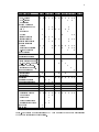
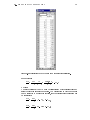
most important features of AQUASIM. Table 1.1 (page 3) gives an overview over which
features are used (x) and which are discussed (X) in the solution of which problem. The
overview given in Table 1.1 may be used to make a personal selection of the
problems to be studied. A problem is recommended to be studied by program users
who are familiar with the features used (x) and interested to learn the features discussed
(X) in this problem. Copies of all les which are created in the tutorial examples are also
delivered with AQUASIM.
A general guideline for the selection of problems to be studied by users not yet familiar
with AQUASIM can be given as follows:
In the problems of chapter 2 the most essential features for simulating simple systems
consisting of mixed reactors are discussed. Because the execution of simulations
and the plot of results is only discussed in detail in these two problems, these
problems must be studied by any AQUASIM user.
In the problems of chapter 3 the application of the data analysis techniques of
AQUASIM are discussed. These are extremely important features of AQUASIM and
the exibility of AQUASIM with respect to the application of these techniques is one of
its major advantages in comparison to other simulation programs. For this reason, these
problems are strongly recommended to be studied. Nevertheless, for program users
which are only interested in obtaining simulation results for their systems, the problems
in this chapter can be omitted.
The problems in chapter 4 demonstrate the most important problems that can occur
during execution of the numerical solution algorithms. AQUASIM uses very robust algorithms so that numerical problems should only rarely occur. Nevertheless, it is important
to know which problems can occur. For this reason, the problems of this section are
recommended to be studied by experienced users of AQUASIM.
In all previous chapters, only mixed reactor compartments were used. The problems
in chapter 5 demonstrate the use of the more complicated compartments of AQUASIM.
In each subsection the application of another compartment is demonstrated. Therefore,
1
2
CHAPTER 1. INTRODUCTION
the problems in this chapter can be selected according to the interest in the
dierent types of compartments.
Finally, the problems in chapter 6 demonstrate how to execute long AQUASIM jobs
on compute servers and how to use AQUASIM in connection with other programs that
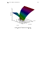
provide parameter sets or postprocess results (e.g. for plotting 2 surfaces or for executing Monte Carlo simulations). These problems are interesting for advanced
AQUASIM users working with large models and computing time intensive
jobs and for users who want to calculate results for parameter sets specied
externally of AQUASIM.
3
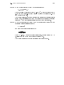
Program feature
State variable:
dyn. volume
dyn. surface
equilibrium
Program variable:
calculation number
time
zone index
others
Constant variable
Real list variable
Variable list variable
Formula variable:
values
algebraic expression
if-then construct
Probe variable
Dynamic process
Equilibrium process
Mixed reactor compart.
Biolm reactor compart.
Adv.-di. react. compart.
Soil column compart.
River section compart.
Lake compartment
Advective link
Diusive link
Simulation
Sensitivity analysis
Parameter estimation
Numerical parameters
Batch mode
Print to le
Plot to screen:
calculated values
data points
error bars
error contributions
sensitivity functions
Plot to le
List to le
2.1 2.2 3.1 3.2 3.3 4.1 4.2 5.1 5.2 5.3 5.4 5.5 6.1 6.2
X x x x x x x x x x x x
X x
X
X
X
X x
X
X x
x x x x
X x x
x
x x
X x
x x
x x x
x
x x x x x x x x
x
x
x x x
X
x
X x x x x x
x
X x x x x x
x
X
X
X x
x
x
x x
X
x
X x
X x
X
x x x
x
X
x
X
X
X
x x x x x x x
X X
X
X x
X x x x x x x x x x x x
X x
X
X
X x
X
X
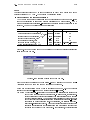
Table 1.1: Overview of which features of AQUASIM are used (x) and which are discussed
(X) in which subsection of this tutorial.
4
CHAPTER 1. INTRODUCTION
Chapter 2
Simulations with Simple Models
In the problems and solutions described in this chapter the most essential features for
simulating simple systems consisting of mixed reactors are discussed. The familiarity of the
user with the program features discussed in this chapter is required for using AQUASIM
and for understanding the solutions to the problems discussed in the other chapters. See
Table 1.1 on page 3 for an overview of which AQUASIM features are discussed in which
section of this tutorial.
In the problem discussed in section 2.1 the focus is on the formulation of processes and
on the execution of simulations and the presentation of results on the screen. Furthermore,
the connection of mixed reactors with diusive links is discussed.
In the problem discussed in section 2.2 the focus is on advective connections of mixed
reactors and on substance separation within these connections. As important additional
features, program variables and real list variables and output of modeling results on
PostScript or ASCII data les are discussed.
5
CHAPTER 2. SIMULATIONS WITH SIMPLE MODELS
6
2.1 Biochemical Processes in a Batch Reactor
Problem
This example demonstrates how to formulate a simple set of biochemical processes in a
batch reactor, how to connect such a reactor diusively to a second reactor, how to do
simulations, and how to plot the results to the screen.
Part A: In a stirred batch reactor with a volume of 10 l a substance A is degraded by a
rst order process with a rate of
rA = kACA
and a rate constant of kA = 1 h,1 (rA denotes the absolute value of the process
rate, CA denotes the concentration of substance A). The initial concentation of
substance A is 1 mg/l.
Plot the concentration of substance A in the reactor as a function of time for a
time interval of 10 h.
Part B: Substance A is not completely degraded but it is converted to substance B
with a xed stoichiometry of 2:1 (1 mg of substance A is converted to 0:5 mg
of substance B ). Substance B is converted to substance C with the nonlinear
transformation rate
CB
rB = rKmax;B
+C
B
B
according to Monod, with a maximum conversion rate of rmax;B = 0:25 mg/l/h
and a half-saturation concentration of KB = 0:5 mg/l (rB denotes the absolute
value of the process rate, CB denotes the concentration of substance B ). The
stoichiometric ratio of this conversion is 1:2 (1 mg of substance B is converted
to 2 mg of substance C ). The initial concentrations of the substances B and C
are zero, the process rate and initial concentration of substance A is the same
as in part A.
Plot the concentrations of the substances A, B and C as functions of time for
a time interval of 10 h.
Part C: The water volume of the reactor of 10 l is now in connection to a closed gas
volume of additional 10 l. Substances A and B are assumed not to exist in the
gas phase but substance C escapes to the gas phase. The non-dimensional Henry
coecient of substance C is given by HC = 2 (the equilibrium concentration of
C in the gas phase is twice as large as the concentration in the water phase). The
gas exchange coecient for substance C with respect to concentrations in the
water phase is given as qex;C = 1 l/h. The initial concentration of the substance
C in the gas volume is zero. The initial concentrations of the substances A, B
and C in the water volume and the process rates of these substances are the
same as in part B.
Plot the concentrations of the substances A, B and C in the water volume as
well as the concentration of substance C in the gas volume as functions of time
for a time interval of 30 h. Check your system denitions on the print le.
2.1. BIOCHEMICAL PROCESSES IN A BATCH REACTOR
7
Solution
Part A
Start the window interface version of AQUASIM or click the command File!New from
the main menu bar to remove previously entered data from memory. Then perform the
following steps:
Denition of variables
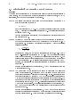
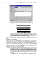
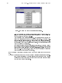
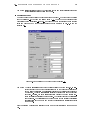
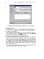
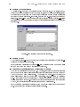
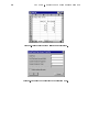
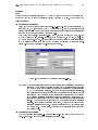
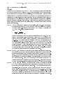
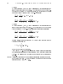
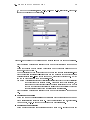
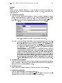
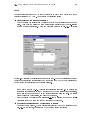
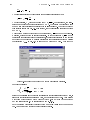
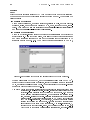
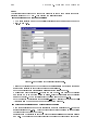
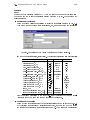
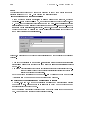
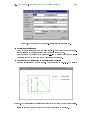
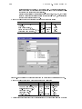
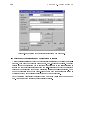
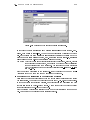
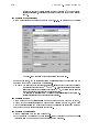
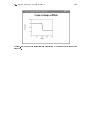
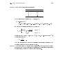
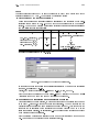
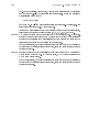
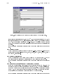
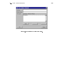
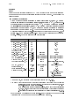
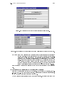
Click the command Edit!Variables or Edit!System from the main menu bar (the
latter command also opens the dialog boxes for editing processes, compartments and
links), click the button New in the dialog box Edit Variables and select the variable
type State Variable as shown in Fig. 2.1. Now dene a state variable C A for the
concentration CA of the substance A as shown in Fig. 2.2.
Figure 2.1: Dialog box for editing variables and selection box of variable type that appears
after selecting the button New.
Comment: Note that the unit of a variable is only a comment that helps the program user to
specify his or her inputs consistently. The user is responsible that this consistency
is guaranteed. AQUASIM only uses the values of the variables and does not
convert automatically between dierent units.
In a batch reactor CA can equivalently be described by a dynamic volume state
variable or by a dynamic surface state variable, because such a reactor has no
throughow. For substances dissolved in the water, however, it is more natural
to describe them by dynamic volume state variables. This is more robust against
errors if later on a throughow or an advective or diusive link is introduced
(surface state variables are not transported in such cases).
8
CHAPTER 2. SIMULATIONS WITH SIMPLE MODELS
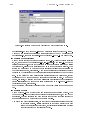
Figure 2.2: Denition of the state variable C A for the concentration CA .
The default accuracies of 10,6 are acceptable because typical concentrations are
in the order of 1 in this example (relative accuracies in the range of 10,6 to 10,4
and absolute accuracies in the range of a fraction of 10,6 to 10,4 of a typical value
are recommended).
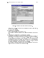
Analogously dene a formula variable k A for the rate constant kA as shown in Fig.
2.3.
Figure 2.3: Denition of the formula variable k A for the rate constant kA .
Comment: The degradation rate constant kA can alternatively be implemented as a constant
variable or as a formula variable. The implementation as a constant variable has
the advantage that the value can be estimated by the parameter estimation algorithm and that sensitivity analyses with respect to the variable can be performed.
If only simulations are to be performed, the specication of model parameters as
formula variables is simpler because no standard deviation and no bounds of the
legal interval of values must be specied. If later on a parameter estimation or a
sensitivity analysis with respect to kA has to be performed, it is very simple by
selecting the variable in the dialog box Edit Variables and clicking the button
Edit Type to change the type of the variable k A to a constant variable.
A constant value is the most trivial example of an algebraic expression used in
a formula variable. Note that any algebraic expression with addition (+), subtraction (-), multiplication (*), division (/), exponentiation (^), and with many
mathematical functions can be used instead (see the user manual for a detailed
2.1. BIOCHEMICAL PROCESSES IN A BATCH REACTOR
9
description of the formula syntax). All previously dened variables can be used in
such an algebraic expression.
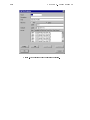
Dene a formula variable C Aini with a value of 1 for the initial condition as shown
in Fig. 2.4.
Figure 2.4: Denition of the variable C Aini for the initial concentration CA;ini.
Comment: It is not necessary to introduce the variables k A and C Aini, because their values
can directly be specied in the rate expression of the dynamic process and as
the initial condition for the variable C A in the denition of the compartment.
However, in most cases it is advantageous to introduce rate constants and initial
conditions as variables. This increases the clarity of the denitions and makes
it easier to use these parameters later on in sensitivity analyses and parameter
estimations (the type of a variable can be changed quickly).
Save your system denitions to the le proc a.aqu by clicking the command File!Save As from the main menu bar and specifying the le name.
Comment: Although program crashes occur very rarely, it is recommended to save system
denitions frequently and to create backup copies of AQUASIM system les.
Denition of process
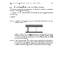
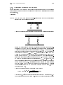
The process matrix for the degradation process in this simple example is given by (see
the user manual for the denition of a process matrix)
Name
Substance Rate
CA
,1
Degradation of A
kACA
Each row of such a process matrix is represented by one dynamic process in AQUASIM
(in this case it contains only one process).
Click the command Edit!Processes or Edit!System from the main menu bar (the
latter command also opens the dialog boxes for editing variables, compartments and
links), click the button New in the dialog box Edit Processes and select the process
type Dynamic Process. Now dene the degradation process given in the above process
matrix as shown in Fig. 2.5. To specify the stoichiometric coecient click the button
Add, select the variable C A and specify the value of -1.
Comment: Note that the process matrix is not unique. Equivalent process matrices would be
CHAPTER 2. SIMULATIONS WITH SIMPLE MODELS
10
Figure 2.5: Denition of the degradation process of substance A.
Name
or
Degradation of A
Name
Substance
Rate
1
,kA CA
CA
Substance Rate
CA
,kA
Degradation of A
CA
However, for rates that do not change their sign, it is usual to make the rate
positive and implement the sign in the stoichiometric coecient. Furthermore,
the stoichiometric coecient of the substance of most interest is set to ,1 or +1,
so that the original matrix is of the recommended form.
Save your system denitions by clicking the command File!Save from the main menu
bar.
Denition of compartment
Click the command Edit!Compartments or Edit!System from the main menu bar
(the latter command also opens the dialog boxes for editing variables, processes and
links), click the button New in the dialog box Edit Compartments and select the compartment type Mixed Reactor Compartment. Now dene the compartment Reactor
describing the batch reactor as shown in Fig. 2.6. The reactor type is selected to be of
constant volume and the volume is set to 10 l.
Comment: For the alternative option of variable volume, the outow would have to be
specied in the edit eld below the radio buttons. Changes in volume would then
be calculated by the program by integration of the dierences in inow (specied
under Input) and outow. The program variable Reactor Volume can be used
to make the outow depend on the current water level in the reactor (for an
explanation of program variables look at Table 1.1 on page 3 to nd an appropriate
example).
The consistent unit of the volume is liters, because the concentration was specied
2.1. BIOCHEMICAL PROCESSES IN A BATCH REACTOR
11
Figure 2.6: Denition of the batch reactor.
with the unit of mg/l. As mentioned previously, AQUASIM only uses the numbers
specied and does not convert units.
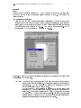
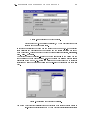
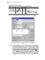
In addition to specifying the volume in the dialog box shown in Fig. 2.6, the relevant
state variables and processes must be activated and the initial condition and input
must be specied. This is done with the four buttons labelled Variables, Processes,
Init. Cond., and Input.
To activate the state variable C A click the button Variables in the dialog box for
the denition of the compartment (Fig. 2.6). In the dialog box Select Active State
Variables shown in Fig. 2.7, select the variable in the right list box of available
variables and click the button Activate (or double-click the variable in the right list
box).
Figure 2.7: Selection of active state variables.
Comment: Note that state variables that are not active in a compartment return a value of
zero. It is an important feature of AQUASIM that state variables can individually
CHAPTER 2. SIMULATIONS WITH SIMPLE MODELS
12
Figure 2.8: Denition of initial condition.
be activated and inactivated in any compartment. This avoids unnecessary computation of state variables which represent substances that are not present in all
compartments. However, sometimes this also leads to errors because the program
user forgot to activate the relevant state variables (only variables of this type need
to be activated). Similarly to variables, processes can also be selectively activated
or inactivated in each compartment.
The process DegradationA is activated analogously. Click the button Processes in the
dialog box for the denition of the compartment (Fig. 2.6). In the dialog box Select
Active Processes select the process in the right list box of available processes and
click the button Activate (or double-click the process in the right list box).
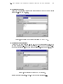
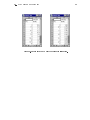
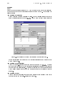
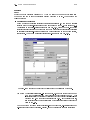
Finally, to specify the initial condition, click the button Init. Cond. in the dialog
box for the denition of the compartment (Fig. 2.6). Now, click the button Add in the
dialog box Edit Initial Conditions shown in Fig. 2.8, select the variable C A and
specify the name of the variable C Aini as the initial condition.
Comment: Note that no input must be specied in this example, because this would be in
contradiction to the denition of a batch reactor. To dene throughow and
substance input uxes in cases where this is necessary, click the button Input and
give these denitions in the dialog box Edit Input.
Save your system denitions by clicking the command File!Save from the main menu
bar.
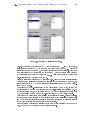
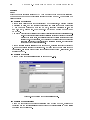
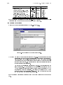
Denition of plot
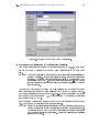
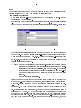
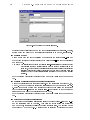
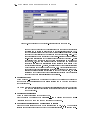
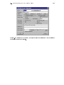
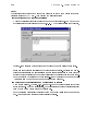
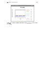
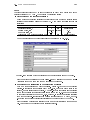
Click the command View!Results from the main menu bar and click the button New
in the dialog box View Results. Now specify the plot denition as shown in Fig. 2.9.
This plot contains a single curve for the value of the variable C A. To dene the curve
for the variable C A click the button Add. Then select the variable C A in the eld
Variable of the dialog box Edit Curve Definition (in the present example, C A is
already selected because it is the rst variable of the list). All other entries can be let
at their default values.
Comment: A plot denition can be specied before or after a simulation has been performed.
It only contains the information of which properties of which variables in which
2.1. BIOCHEMICAL PROCESSES IN A BATCH REACTOR
13
Figure 2.9: Denition of plot for the variable C A.
compartment and at which location are to be plotted and which signatures are to
be used. After successful completition of a simulation, the plot denition can be
used for the generation of the plot based on the data of the simulation. After a
repetition of the simulation with changed parameter values, the same plot denition can be used to display a plot for the new simulation. The window containing
the old plot is not aected by this procedure.
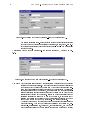
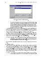
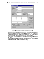
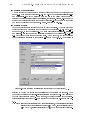
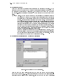
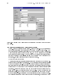
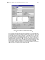
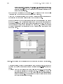
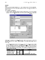
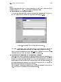
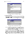
Denition of the simulation
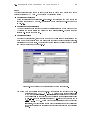
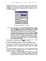
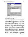
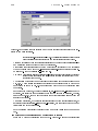
To dene the simulation click the command Calc!Simulation in the main menu bar.
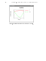
This dialog box Simulation shown in Fig. 2.10 is then used to dene calculations and
to initialize, start and continue the simulation. Simulations consist of one or more
calculations. The buttons Initialize and Start/Continue in this dialog box are
inactive unless at least one calculation is dened and is active (as is already the case
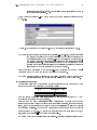
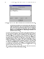
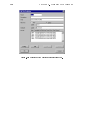
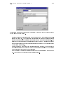
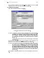
in Fig. 2.10). Now click the button New in this dialog box. The dialog box shown in
Fig. 2.11 appears. Accept the default values of 0 for the Calc. Number and for the
Initial Time and the default selection for the Initial State. Write 0.1 in the edit
eld Step Size and 100 in the edit eld Num. of Steps below the list box Output
Steps and click Add. This copies these entries to the list box for step sizes and numbers
of steps. Finally, select the calculation to be active for simulation. The dialog box
Edit Calculation Definition should now look as shown in Fig. 2.11.
Comment: Note that the step size chosen in the dialog box shown in Fig. 2.11 species which
states are stored in memory for plotting. 100 steps seem to give a good enough
resolution of the plot over the duration of 10 h. The internal step size selected by
the integration algorithm depends on the accuracy of the state variables (cf. Fig.
14
CHAPTER 2. SIMULATIONS WITH SIMPLE MODELS
Figure 2.10: Dialog box used for controlling simulations.
2.2). One calculation can consist of several series of steps of dierent size. Each
series of a number of steps of constant size is represented by one row in the list
box of the dialog box shown in Fig. 2.11.
Each calculation has a calculations number. Only calculations that dier in the
value of the calculation number can be active simultaneously. The program variable Calculation Number returns the value specied here (for an explanation of
program variables look at Table 1.1 on page 3 to nd an appropriate example).
For this reason, with the aid of this program variable, the model equations can be
made to depend on the calculation.
If the steady state option for the initial state is selected, the program tries to
nd the steady state and uses it as an initial state. Note, however, that not for all
systems a steady state exists and that even if it exists, the program may not be
able to nd it. In the latter case, the steady state can be calculated by relaxation
(time integration under constant conditions).
Save your system denitions by clicking the command File!Save from the main menu
bar.
Comment: It is always recommended to save the system denitions before starting a simulation, because simulations may require signicant computation time and because
the cause of a program crash cannot be found without the system le in the version
that was used to start the simulation.
2.1. BIOCHEMICAL PROCESSES IN A BATCH REACTOR
15
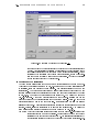
Figure 2.11: Dialog box used for dening a calculation.
Execution of the simulation and presentation of results
Click Start/Continue in the dialog box Simulation shown in Fig. 2.10 (this dialog
box can be opened by clicking the command Calc!Simulation in the main menu
bar).
Comment: Note that if no calculated states exist the button Start/Continue initializes and
starts the simulation. If there exist calculated states, this button continues the
simulation. So clicking Start/Continue again, leads to a continuation of the
simulation to a time of 20 h. In order to repeat the simulation (e.g. with changed
parameter values) the button Initialize must be clicked rst, followed by clicking
Start/Continue.
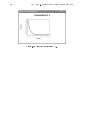
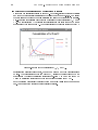
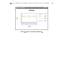
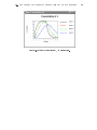
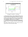
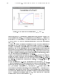
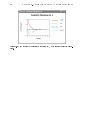
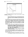
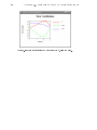
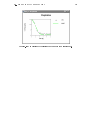
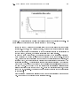
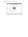
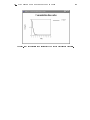
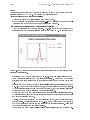
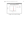
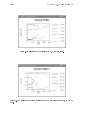
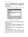
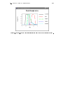
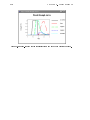
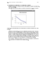
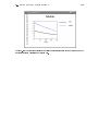
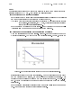
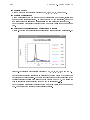
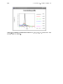
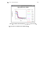
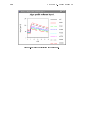
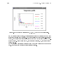
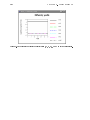
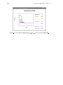
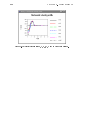
Now select the plot Conc in the dialog box View Results and then click the button
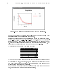
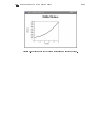
Plot to Screen (the dialog box View Results can be opened by clicking the command View!Results in the main menu bar). Fig. 2.12 shows the resulting plot of the
time course of the concentration CA . The concentration CA decreases exponentially
from its start value of 1 mg/l.
Save your system denitions by clicking the command File!Save from the main menu
bar. Answer No to the question to save calculated states.
Comment: Usually the le size increases unnecessarily when the calculated states are saved,
because the states can readily be recalculated (all system denitions are saved).
An exception is if you want to be able to plot results immediately after loading
the le without performing a simulation. This is only possible if the calculated
states have been saved.
16
CHAPTER 2. SIMULATIONS WITH SIMPLE MODELS
Figure 2.12: Plot of the concentration CA .
2.1. BIOCHEMICAL PROCESSES IN A BATCH REACTOR
17
Part B
Continue just after doing part A or load the le saved in part A from within the window
interface version of AQUASIM. Then perform the following steps:
Denition of variables
Dene additional state variables C B for the concentration CB of substance B and C C
for the concentration CC of substance C analogously to the deniton of C A as shown
in Fig. 2.2.
Comment: Instead of clicking the button New in the dialog box Edit Variables and specifying
all entries of the new state variable it is possible to select the variable C A in the list
box of this dialog box and click the button Duplicate. Then only minor changes
must be made in order to dene the new state variables C B and C C.
Analogously to the denition of C Aini shown in Fig. 2.3, dene additional formula
variables rmax B and K B with values of 0:25 mg/l/h and 0:5 mg/l, respectively, for the
process parameters rmax;B and KB .
Denition of processes
The extended process matrix for part B is given by (see user manual for the denition
of a process matrix)
Name
Substance Rate
CA CB CC
Conversion A ! B ,1 12
kACA
Conversion B ! C
,1 2 rmax;B K C+B C
B
B
The rst process in this matrix is an extension of the process dened in part A (not
only degradation of the substance A but conversion of A to B ), the second process is
an additional process. The implementation of the rst process is done by editing the
Figure 2.13: Denition of the conversion process of substance A to B .
degradation process for the substance A shown in Fig. 2.5 to the form shown in Fig.
CHAPTER 2. SIMULATIONS WITH SIMPLE MODELS
18
2.13. To do this, select the process DegradationA in the dialog box Edit Processes
and click the button Edit. Then change the process denitions as shown in Fig. 2.13.
Dene a second new process according to the above process matrix as shown in Fig.
2.14.
Figure 2.14: Denition of the conversion process of substance B to C .
Comment: Note that equivalent process matrices are given by
Name
Substance
Rate
or
CA CB CC
1k C
Conversion A ! B ,2 1
2 A A
Conversion B ! C
,1 2 rmax;B K C+B C
B
B
Name
Substance
Rate
CA CB CC
1k C
Conversion A ! B ,2 1
2 A A
Conversion B ! C
, 12 1 2rmax;B K C+B C
B
B
Both of these matrices fulll the requirements stated in part A. The dierence is
that the stoichiometric coecient with the value of one is assigned to a dierent
substance.
Save your system denitions to the le proc b.aqu by clicking the command File!Save
As from the main menu bar and specifying the le name.
Denition of compartment
Open the dialog box for editing the compartment Reactor dened in part A. Click
the button Variables and activate the new state variables C B and C C. Click now the
button Processes and activate the new process Conversion BC.
2.1. BIOCHEMICAL PROCESSES IN A BATCH REACTOR
19
Comment: Initial conditions have not to be specied for the new state variables because the
default initial conditions of zero can be used.
Denition of plot
Open the dialog box for editing the plot Conc dened in part A. Edit the curve denition
for the variable C A by adding the legend entry C A. Then add two additional curve
denitions for the variables C B and C C. In these two curve denitions change the line
style and color and add the appropriate legend entry as shown in Fig. 2.15 for the
variable C C.
Figure 2.15: Denition of the curve for the variable C C.
Comment: The entry Parameter in the curve denition dialog box shown in Fig. 2.15 is inactive because the type of the curve is selected to be the value of the variable and
not an error contribution or a sensitivity function of a variable with respect to
a parameter. The entry Compartment is inactive because only one compartment
is dened. Finally, the entry Zone is inactive because the mixed reactor compartment Reactor consists of only one zone. The default value of the calculation
number is zero. The calculation number can be used to hold dierent calculations
simultaneously in the memory and to plot the results of such calculations within
the same plot.
Save your system denitions by clicking the command File!Save from the main menu
bar.
20
CHAPTER 2. SIMULATIONS WITH SIMPLE MODELS
Execution of the simulation and presentation of results
Repeat now the simulation performed in part A. To do this, click the button Initialize
and then the button Start/Continue in the dialog box shown in Fig. 2.10. Now select
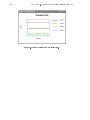
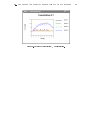
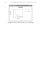
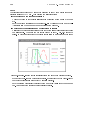
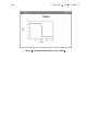
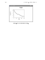
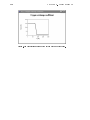
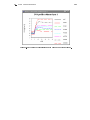
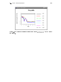
the plot Conc in the dialog box View Results and click the button Plot to Screen.
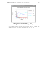
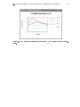
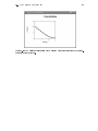
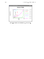
Fig. 2.16 shows the resulting plot of the time courses of the concentrations CA , CB and
CC . The concentration CA decreases exponentially from its start value of 1 mg/l as
it was already the case in part A. The concentration of the intermediate product CB
Figure 2.16: Plot of the concentration CA , CB and CC .
increases from its start value of zero, comes to a maximum and then decreases again
to zero. The concentration of the end product CC raises to the start value of 1 mg/l
of substance A because the stoichiometric ratio of 0.5 from A to B and of 2 from B to
C lead to a stoichiometric factor of 1 for the combined reaction from A to C .
Save your system denitions by clicking the command File!Save from the main menu
bar. Answer No to the question to save calculated states.
2.1. BIOCHEMICAL PROCESSES IN A BATCH REACTOR
21
Part C
Continue just after doing part B or load the le saved in part B from within the window
interface version of AQUASIM. Then perform the following steps:
Denition of variables
Dene additional formula variables H C and qex C with values of 2 and 1 l/h for the gas
exchange parameters HC and qex;C analogously to the denition of C Aini as shown
in Fig. 2.3.
Denition of compartments
Add an additional mixed reactor compartment GasVolume with a bulk volume of 10 l
by clicking the button New in the dialog box Edit Compartments. Activate the state
variable C C in this compartment.
Denition of links
To dene the diusive link, click the command Edit!Links or Edit!System from the
main menu bar (the latter command also opens the dialog boxes for editing variables,
processes and compartments). Then click the button New in the dialog box Edit Links
and dene the link as shown in Fig. 2.17
Figure 2.17: Denition of the diusive link between the reactors.
Comment: With the denition shown in Fig. 2.17 the exchange ux between the compartments is given as qex;C (CC;gas =HC , CC;water ) (from the compartment GasVolume
to the compartment Reactor). Note that selecting Reactor as compartment
1 and GasVolume as compartment 2 and replacing the Exchange Coefficient
by qex C/H C and the Conversion Factor by H C leads to an exchange ux of
qex;C (C
HC C;water , HC CC;gas ) (from the compartment Reactor to the compartment
GasVolume), what is obviously the same as the denition given above (please look
at the user manual for the denition of the exchange coecient and the conversion
factor).
CHAPTER 2. SIMULATIONS WITH SIMPLE MODELS
22
Denition of plot
Open the dialog box for editing the plot Conc dened in part B. Then add an additional
curve denition for the variable C C evaluated in the compartment GasVolume. Add
a legend entry and select an appropriate signature. Click the button Scaling and
specify the scaling parameters as shown in Fig. 2.18.
Figure 2.18: Specication of plot scaling.
Denition of the simulation
Open now the dialog box Simulation shown in Fig. 2.10, select the calculation and
click Edit (or double-click the calculation). In the dialog box shown in Fig. 2.11 select
the row of the list box with the denition of calculation steps and change the value in
the edit eld Num. of Steps below the list box from 100 to 300. Now click Replace.
Save your system denitions to the le proc c.aqu by clicking the command File!Save
As from the main menu bar and specifying the le name.
Execution of the simulation and presentation of results
To start now the simulation click the button Initialize and then the button Start/Continue in the dialog box Simulation shown in Fig. 2.10.
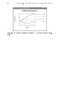
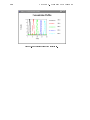
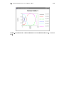
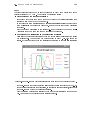
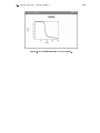
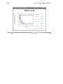
Now select the plot Conc in the dialog box View Results and click the button Plot
to Screen. Fig. 2.19 shows the resulting plot of the time courses of the concentrations
CA, CB and CC in the water volume and of the concentration CC in the gas volume.
The concentrations CA and CB behave as in part B, but CC escapes to the gas phase.
At the end of the simulation, the concentration CC in the gas phase is about twice as
large as that in the water phase as it is expected from the value of the Henry coecient.
Save your system denitions by clicking the command File!Save from the main menu
bar. Answer No to the question to save calculated states.
Now click the command File!Print to File from the main menu bar and specify
a le name. All system denitions are now written to this le in text format. This le
can be printed directly or it can be opened with any text processing program and can
then be printed from this program. This listing is very important in order to check the
system denitions. For cases in which this listing is extremely long, a shorter version
2.1. BIOCHEMICAL PROCESSES IN A BATCH REACTOR
23
Figure 2.19: Plot of the concentration CA , CB and CC .
can be printed by selecting the short le format in the dialog box appearing after
clicking the command File!Print Options from the main menu bar.
CHAPTER 2. SIMULATIONS WITH SIMPLE MODELS
24
2.2 Transport and Substance Separation in a Box Network
Problem
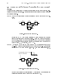
This example demonstrates how to describe advective links between mixed reactors, bifurcations and substance separation. In addition it gives an introduction to program variables
and real list variables.
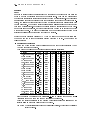
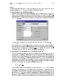
Part A: Look at the conguration of mixed reactors and the ow scheme shown in Fig.
2.20.
10 l/h
10 l
10 l
10 l
1
2
4
3
1l
5 l/h
50 l/h
Figure 2.20: Flow scheme for part A.
Implement an AQUASIM system consisting of mixed reactors and advective
links that corresponds to this conguration. Dene the water ows indicated
in the gure, perform a dynamic calculation over 10 h and plot the discharges
and the retention times in all four reactors (the retention time is given as the
ratio of volume, V , to discharge, Q: = V=Q).
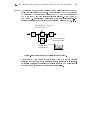
Part B: A substance A ows into the mixed reactor 1 at a concentration as shown in
Fig. 2.21: The inow concentration is 10 mg/l between 0 and 4:9 h, it decreases
linearly from 10 mg/l to 0 between 4:9 and 5:1 h, and it remains at 0 after 5:1 h.
Concentration of sub- 10 mg/l
stance A in the inlet:
5h
1
2
10 h
4
3
Figure 2.21: Substance input for part B.
Plot the time course of the concentration CA of substance A in all reactors for
initial concentrations of zero during a time interval of 10 h.
2.2. TRANSPORT AND SUBSTANCE SEPARATION IN A BOX NETWORK
25
Part C: A substance B now ows into the reactor 3 with a periodic loading of 100 mg/h
during the last quarter of each hour. The substances A and B are converted
to a substance C in reactor 2 at a rate of kAB CA CB with a rate constant of
kAB = 100 l/mg/h and with stoichiometric coecients of ,1 for CA and CB
and +2 for CC . The substance C is separated in the outlet of reactor 2 (e.g. by
settling or ltration) so that it only ows to reactor 4 as shown in Fig. 2.22.
Transformation of A+B to C
with a rate of kAB CA CB
1
2
3
Periodic input
of substance B:
4
C is not transported
through these links
100 mg/h
1h 2h 3h ....
Figure 2.22: Substance input and transformation for part C.
Extend the AQUASIM system dened in part A and B to the new features
described above and plot the time series of all three substances in all reactors.
In addition to plotting the results to the screen plot them to a PostScript le
and export them in text format for external postprocessing.
CHAPTER 2. SIMULATIONS WITH SIMPLE MODELS
26
Solution
Part A
Start the window interface version of AQUASIM or click the command File!New from
the main menu bar to remove previously entered data from memory. Then perform the
following steps:
Denition of variables
Dene three formula variables Qin for the inow, Qin , to compartment 1 with a value
of 10 l/h, Qrec for the recirculation ow, Qrec, from compartment 2 to compartment 3
with a value of 50 l/h, and Qout for the ow, Qout , out of compartment 2 that leaves
the modelled system with a value of 5 l/h.
Comment: It is not necessary to dene these variables because the numbers given in Fig. 2.20
can be entered directly as inows and bifurcation ows (as will become clear later
on). However, in most cases it is recommendable to introduce such auxiliary quantities as variables and use the variables in the inow and bifurcation denitions,
because this makes the system denitions clearer and it facilitates to use these
variables for sensitivity analyses and parameter estimations later on (the type of
a variable can be changed easily).
Dene two program variables Q as Discharge and V as Reactor Volume. As an example
Fig. 2.23 shows the denition of the program variable for discharge.
Figure 2.23: Denition of the program variable for discharge.
Comment: Program variables make quantities used by the program (in this case the discharge
and the reactor volume) available for use in model formulations and for plotting.
Finally, dene a formula variable tau as the algebraic expression V/Q
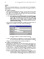
Denition of compartments and links
Before starting the implementation of compartments and links it must be clear how the
investigated system should be mapped to an AQUASIM conguration. Fig. 2.24 shows
how this is done in this example. All four mixed reactors are mapped to mixed reactor
compartments of AQUASIM. The connections from reactor 1 to 2, from reactor 2 to
4 and from reactor 3 to 2 are mapped as advective links, the connection from reactor
2 to reactor 3 and the connection that leaves the modelled system from reactor 2 are
implemented as bifurcations from the advective link from reactor 2 to 4.
Comment: Note that the denition of links and bifurcations is not unique. Any of the three
connections leaving the reactor 2 could be mapped to an advective link with the
other two implemented as bifurcations. Because for each bifurcation a water ow
2.2. TRANSPORT AND SUBSTANCE SEPARATION IN A BOX NETWORK
Reactor 1
Reactor 4
Reactor 2
Link 12
27
Link 24
Bifurcation Out
Link 32
Bifurcation Rec
Reactor 3
Figure 2.24: Mapping of the reactor conguration to AQUASIM.
can be specied and the rest of the water ows through the link that contains the
bifurcations, with the data available, it seems to be most natural to dene the
connection from reactor 2 to 4 as the link and the other two as the bifurcations.
Dene now four mixed reactor compartments Reactor 1, Reactor 2, Reactor 3 and
Reactor 4 with volumes of 10 l, 10 l, 1 l and 10 l, respectively. For the compartment
Reactor 1 dene Qin as the water inow (click the button Input in the dialog box
for the denition of the compartment and write the expression Qin in the edit eld
labelled Water Inflow).
Dene now three advective links Link 12 from the compartment Reactor 1 to the
compartment Reactor 2, Link 32 from the compartment Reactor 3 to the compartment Reactor 2 and Link 24 from the compartment Reactor 2 to the compartment
Reactor 4. For the link Link 24 dene two bifurcations Rec with a water ow of Qrec
to compartment Reactor 3 and Out with a water ow Qout and without an outow
compartment. As an expample Fig. 2.25 shows the denition of the link Link 24 and
Figure 2.25: Denition of link from reactor 2 to reactor 4.
Fig. 2.26 shows the denition of the bifurcation Rec.
CHAPTER 2. SIMULATIONS WITH SIMPLE MODELS
28
Figure 2.26: Denition of recirculation as a bifurcation of an advective link.
Denition of plots
Dene two plots Q and tau each of which contains four curves for the discharge Q and
the retention time tau evaluated in each of the four compartments, respectively.
Denition of the simulation
Dene a calculation of 100 steps of size 0:1 h as described in section 2.1 (Fig. 2.11).
Save your system denitions to the le flow a.aqu by clicking the command File!Save
As from the main menu bar and specifying the le name.
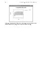
Execution of the simulation and presentation of results
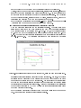
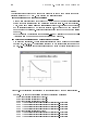
To start the simulation click the button Start/Continue in the dialog box Simulation
openend with the command Calc!Simulation. Then use the plot denitions Q and
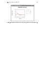
tau to plot discharges and retention times. Figure 2.27 shows the plot of the discharges
and Fig. 2.28 that for the retention times in all four reactors. As is evident from Fig.
2.20 the discharge is 10 l/h for reactor 1, 60 l/h for reactor 2, 50 l/h for reactor 3, and
5 l/h for reactor 4. The retention times of reactors 2 and 3 are much smaller than
those of the reactors 1 and 4.
Save your system denitions by clicking the command File!Save from the main menu
bar. Answer No to the question to save calculated states.
2.2. TRANSPORT AND SUBSTANCE SEPARATION IN A BOX NETWORK
Figure 2.27: Plot of discharge in all reactors.
29
30
CHAPTER 2. SIMULATIONS WITH SIMPLE MODELS
Figure 2.28: Plot of retention time in all reactors.
2.2. TRANSPORT AND SUBSTANCE SEPARATION IN A BOX NETWORK
31
Part B
Continue just after doing part A or load the le saved in part A from within the window
interface version of AQUASIM. Then perform the following steps:
Denition of variables
Dene a state variable C A for the concentration CA of substance A and a program
variable t for time. Then dene a real list variable for the input concentration C Ain
as shown in Fig. 2.29. To add the data pairs specify the numbers for argument and
Figure 2.29: Denition of the real list variable for CA;in .
value in the edit elds below the list box and then click the button Add.
Comment: For values of the argument within the range of arguments of data pairs the value of
the real list variable is interpolated or smoothed according to the method selected
with the radio buttons in the dialog box shown in Fig. 2.29. For both interpolation
techniques, outside of this range the value of the rst or last data point is used.
For this reason, omission of the rst data pair in the dialog box shown in Fig. 2.29
would lead to the same result.
The integration algorithm used by AQUASIM is not able to step over discontinuities of input variables. For this reason, an input concentration that would
discontinuously switch from 10 mg/l to zero would result in numerical problems.
Such an input must be approximated by an input as used in Fig. 2.29 that switches
continuously from one value to another. However, the width of this transient range
could be made much smaller.
CHAPTER 2. SIMULATIONS WITH SIMPLE MODELS
32
Denition of compartments
The variable C A must now be activated in every compartment. To do this, open the
dialog box for the denition of every compartment, click the button Variables, select
the variable in the right list box of the dialog box Select Active State Variables
and click the button Activate. In addition, as shown in Fig. 2.30, for the compartment
Reactor 1, Qin*C Ain must be specied as the input loading for the variable C A. Initial
conditions have not to be specied because the default initial condition of zero is correct
in this case.
Figure 2.30: Denition of the input to reactor 1.
Denition of plot
An additional plot C A must be dened that contains four curves for the variable C A
evaluated in all four compartments.
Save your system denitions to the le flow b.aqu by clicking the command File!Save
As from the main menu bar and specifying the le name.
Execution of the simulation and presentation of results
Redo now the simulation done in part A. To do this, click rst the button Initialize
and then the button Start/Continue of the dialog box Simulation that can be opened
with the command Calc!Simulation. Then select the plot C A in the dialog box
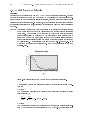
View Results and click the button Plot to Screen. Fig. 2.31 shows the resulting
plot. This gure shows how the substance A enters the system and is washed out after
its elimination from the input. Because of the very short retention time in the reactors
2 and 3, the concentrations in these reactors cannot be distinguished.
Save your system denitions by clicking the command File!Save from the main menu
bar. Answer No to the question to save calculated states.
2.2. TRANSPORT AND SUBSTANCE SEPARATION IN A BOX NETWORK
Figure 2.31: Plot of concentration CA in all reactors.
33
CHAPTER 2. SIMULATIONS WITH SIMPLE MODELS
34
Part C
Continue just after doing part B or load the le saved in part B from within the window
interface version of AQUASIM. Then perform the following steps:
Denition of variables
Dene state variables C B for the concentration CB of substance B and C C for the
concentration CC of substance C .
In order to simplify the denition of a periodic input function, dene a formula variable
t fract that returns the fraction of an hour. As shown in Fig. 2.32 this can be done by
use of the modulo function which returns the rest after integer division. Within each
Figure 2.32: Denition of time as a fraction of an hour.
hour this function increases linearly from 0 to 1 and jumps back to 0 at the beginning of
the next hour. Now dene a real list variable F Bin for the input loading of substance
B into the reactor 3 as shown in Fig. 2.33. Note that the variable t frac is used here
as an argument instead of t as used for the inow concentration of substance A shown
in Fig. 2.29. Because of the denition of t frac this makes the time course of this
variable periodic with period 1 h.
Comment: Note that the discontinuity of the variable t frac after each hour may cause a
discontinuity of a real list for which this variable is used as an argument. Because
the integration algorithm used by AQUASIM has problems to step over discontinuities in input functions or process rates, this must be avoided. In the current
context this is most easily avoided by ending the real list with argument t frac
with the same value at the end of the period (in this case at 1) as was the start
value at 0.
Look at the user manual for the functions available in formula variables and for
the syntax of algebraic expressions.
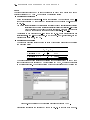
Instead of typing the data pairs in the edit elds below the list box of the dialog box
shown in Fig. 2.33 and clicking the button Add, it is possible to read data pairs from
a text le. In many cases data may be available in a spreadsheet as shown in Fig.
2.34. In order to make such a le readable by AQUASIM save the spreadsheet in
text format. AQUASIM can read data pairs from given rows and columns of a text
le. Spaces between numbers (or text), tabs and commas are interpreted as column
delimiters by AQUASIM. To read the data click the button Read in the dialog box
shown in Fig. 2.33, select the le name and specify the row and column numbers in
the dialog box shown in Fig. 2.35. For the data shown in Fig. 2.34 start and end row
are 4 and 8 (or zero for end of le), the column number of the argument is 2, and the
2.2. TRANSPORT AND SUBSTANCE SEPARATION IN A BOX NETWORK
35
Figure 2.33: Denition the real list variable for input of B .
column number of the value is 3 as shown in Fig. 2.35 if the spreadsheet is stored with
tabs or commas as eld delimiters. If the spreadsheet is stored with spaces as eld
delimiters, the leading empty column cannot be distinguished from leading blanks so
that the column number of the argument would be 1, that of the value 2.
Finally, implement the rate constant KAB as a formula variable k AB with a value of
100 l/mg(h.
Save your system denitions to the le flow c.aqu by clicking the command File!Save
As from the main menu bar and specifying the le name.
36
CHAPTER 2. SIMULATIONS WITH SIMPLE MODELS
Figure 2.34: Input loading time series on a spreadsheet.
Figure 2.35: Dialog box for reading data pairs from a le.
2.2. TRANSPORT AND SUBSTANCE SEPARATION IN A BOX NETWORK
37
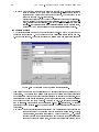
Denition of process
Dene now the conversion process taking place in reactor 2 as the dynamic process
Production C shown in Fig. 2.36.
Figure 2.36: Denition the process of conversion of A and B to C .
Denition of compartments
Activate now the state variables C B and C C and the process Production C in the
compartment Reactor 2, activate the state variable C B and dene the variable F Bin
as the input loading for C B in the compartment Reactor 3 as shown in Fig. 2.37, and
Figure 2.37: Denition of the input of B to reactor 3.
activate the state variables C B and C C in the compartment Reactor 4.
CHAPTER 2. SIMULATIONS WITH SIMPLE MODELS
38
Comment: The water inow specied in the dialog box shown in Fig. 2.37 is only the external
inow in addition to the inow from advective links. Because there is only a
substance input without an accompanying water ow, the water inow in the
dialog box shown in Fig. 2.37 is set to zero.
Because the substances B and C cannot be present in the compartment Reactor 1,
it is not necessary to activate the state variables C B and C C in this compartment. Similarly the state variable C C has not to be activated in the compartment
Reactor 3 (not activating these state variables increases the computation speed,
because AQUASIM has a smaller number of dierential equations to solve).
Denition of links
The bifurcations Rec and Out of the advective link Link 24 must be modied not to
transport the substance C . For the example of the bifurcation Rec it is shown in Fig.
2.38 how this is done. The radio buttons with water flow and as given below of
Figure 2.38: Modication of the denition for recirculation.
this dialog box are used for the selection of how substance loadings are divided at the
bifurcation. The default with water flow leads to a division of substance loadings
proportional to water ow as it is typical for dissolved or suspended substances. If the
alternative as given below is selected, the substance loadings can be given explicitly
in the list box below the radio buttons. As shown in Fig. 2.38 loadings of Qrec*C A
and of Qrec*C B were specied for the variables C A and C B, respectively. No loading
is specied for the variable C C so that the substance C is not transported through the
bifurcation.
Comment: Note that the loadings for the substances A and B as specied above are exactly the
same as those used by the program with the option with water flow. However,
with this option, the loading of substance C would be given as QrecCC . Also in
the case that only one substance loading must be changed from its default value
under the option with water flow, the radio button as given below must be
2.2. TRANSPORT AND SUBSTANCE SEPARATION IN A BOX NETWORK
39
selected and all nonzero loadings must be specied. For this specication, the
program variable Discharge can be used. In the context of a bifurcation of an
advective link, this program variable returns the total water inow to the link.
Dene now substance loadings of Qout*C A and Qout*C B for the variables C A and C B
in the bifurcation Out in the same way.
Denition of plot
Add now two additional plot denitions C B and C C each containing curves for the
concentration of the corresponding substance in all four reactors.
Comment: This can be done by selecting the plot C A and then clicking the button Duplicate.
The changes from C A to C B or C C need then less editing compared to creating
new plot denitions.
Save your system denitions by clicking the command File!Save from the main menu
bar.
Execution of the simulation and presentation of results
Redo now the simulation done in parts A and B. To do this, rst click the button
Initialize and then the button Start/Continue of the dialog box Simulation that
can be opened with the command Calc!Simulation. Then plot the concentrations
of all three substances by selecting the appropriate plot denition and then clicking
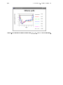
the button Plot to Screen in the dialog box View Results. The results are shown
in the Figs. 2.39, 2.40 and 2.41. The rst plot (as compared to Fig. 2.31 without
Figure 2.39: Plot of concentration CA in all reactors.
conversion process) shows the consumption of substance A during the intervals in
which the substance B is added. The second plot mainly shows the periodic input
of substance B . The concentration of B increases after 8 hours because then the
substance A is consumed and the conversion process of A and B to C does not longer
take place. Finally, the last plot shows the increase and decrease of the concentration
of the substance C .
40
CHAPTER 2. SIMULATIONS WITH SIMPLE MODELS
Figure 2.40: Plot of concentration CB in all reactors.
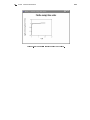
Now select the rst plot denition in the dialog box View Results and click the button
Plot to File and specify a le name. Repeat this procedure for the other two plot
denitions and specify the same le name. All plots are now plotted to this PostScript
le which can be sent to a printer in a way that depends on the hard- and software of
the computer in use. A universal way is to load the PostScript le with the shareware
program GhostScript and print it using the menu of this program.
Redo the same steps with clicking the button List to File instead of Plot to File
and with specifying another le name. This le contains now all data series in text
format. It can be loaded by any spreadsheet or plot program for external postprocessing.
Save your system denitions by clicking the command File!Save from the main menu
bar. Answer No to the question to save calculated states.
2.2. TRANSPORT AND SUBSTANCE SEPARATION IN A BOX NETWORK
Figure 2.41: Plot of concentration CC in all reactors.
41
42
CHAPTER 2. SIMULATIONS WITH SIMPLE MODELS
Chapter 3
Application of Data Analysis
Techniques
The tutorial examples discussed in this chapter are designed to give an introduction to the
data analysis techniques of AQUASIM. This is the only chapter where these techniques
are discussed. Because of the importance of these techniques it is strongly recommeded
for any AQUASIM user to study the examples given in this chapter carefully. See Table
1.1 on page 3 for an overview of which AQUASIM features are discussed in which section
of this tutorial.
The problem discussed in section 3.1 gives an introduction in the calculation and use
of sensitivity functions for identiability analysis. In addition, constant variables are
introduced, which are very important for the whole chapter.
In section 3.2 the most important data analysis features of AQUASIM are discussed:
Parameter estimations, sensitivity analyses and error analyses. In addition, the use of
variable list variables is discussed. This is also very important, because similar uses are
advantageous in many contexts.
The last example in section 3.3 does not introduce new program features, but it demonstrates how AQUASIM can be used to make model structure selections.
43
44
CHAPTER 3. APPLICATION OF DATA ANALYSIS TECHNIQUES
3.1 Identiability Analysis with Sensitivity Functions
Problem
This example demonstrates the usefulness of sensitivity functions in order to assess the
identiability of model parameters.
Part A: In a stirred batch reactor with a volume of 10 l there are three substances A,
B and C that interact according to the following process matrix (if you have
problems to understand the meaning of a process matrix see the user manual
and the example described in section 2.1. In part B of this example exactly the
same process matrix was used):
Name
Substance
Rate
CA CB CC
kACA
Conversion A ! B ,1 12
Conversion B ! C
,1 2 rmax;B K C+B C
B
B
The process parameters are given as kA = 1 h,1 , rmax;B = 0:25 mg/l/h and
KB = 0:5 mg/l. The initial concentration of substance A is CA;ini = 1 mg/l,
the initial concentrations of the other two substances are zero.
Plot the concentrations of all three substances in the reactor and the sensitivity
functions
a;r = p @y
y;p
@p
for all concentrations y = CA , CB and CC with respect to the parameters
p = CA;ini, kA, rmax;B and KB as functions of time for a time interval of 10 h.
Use these sensitivity functions to assess the identiability of model parameters
from measured time series of the concentrations CA , CB and CC .
Part B: Use the sensitivity functions plotted in part A to determine which of the other
parameters must be changed to which value if KB is increased by a factor of 2 to
KB = 1 mg/l in order to obtain a similar result as with the previous parameter
values. Perform the simulations for the new set of parameters and compare it
with the simulation done in part A.
3.1. IDENTIFIABILITY ANALYSIS WITH SENSITIVITY FUNCTIONS
45
Solution
Part A
Start the window interface version of AQUASIM or click the command File!New from
the main menu bar to remove previously entered data from memory. Then perform the
following steps:
Denition of variables
Dene the dynamic volume state variables C A, C B and C C for the concentrations CA
of substance A, CB of substance B and CC of substance C . Let the accuracies at their
default values of 10,6 (recommendations with respect of the values of these accuracies
are given in the example described in section 2.1).
Then dene four constant variables C Aini for CA;ini with a value of 1 mg/l, k A for
kA with a value of 1 h,1, rmax B for rmax;B with a value of 0:25 mg/l/h, and K B for
KB with a value of 0:5 mg/l. Set the standard deviation of each of these variables to
10 % of its value and set the minimum and maximum to zero and 10 times the value.
Figure 3.1 shows the denition of C Aini as an example.
Figure 3.1: Denition of the constant variable C Aini.
Comment: The partial derivatives required for the calculation of sensitivity functions are
calculated by comparing the results obtained with the original parameter value
and those obtained with a parameter value that deviates from the original value
by 1 % of its standard deviation. In order that this gives reasonable results,
this deviation in the parameter must lead to deviations in the results that are
small enough that the secant gives a reasonable approximation to the tangent
of the solution (negligible nonlinearity of the model response with respect to the
parameter) but large enough that the deviation is larger than numerical integration
errors. 1 % of the standard deviation seems to be a reasonable value to fulll this
criterion. If the standard deviation is unknown, a value must be assumed that
fullls the criterion given above. A standard deviation of 10 % of the value leads
to a change of 0.1 % of the value, what seems to be reasonable if the value is not
very close to zero.
Denition of processes
The two processes Conversion AB and Conversion BC are dened as shown in the
Figs. 2.13 and 2.14 of the example discussed in section 2.1.
46
CHAPTER 3. APPLICATION OF DATA ANALYSIS TECHNIQUES
Denition of compartment
A mixed reactor compartment with a constant volume of 10 l must be dened as shown
in Fig. 2.6. Then the state variables C A, C B and C C and the processes Conversion AB
and Conversion BC must be activated with the aid of the dialog boxes opened by
clicking the buttons Variables and Processes, respectively. Finally, C Aini must be
specied as the initial condition for the state variable C A with the aid of the dialog
box opened by clicking the button Init. Cond. as shown in Fig. 2.8.
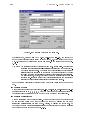
Denition of plots
Four plot denitions are required in order to plot the results. The rst plot Conc
contains three curve denitions for the values of the variables C A, C B and C C as
shown in Fig. 2.15 for the variable C C. The three plot denitions SensAR A, SensAR B
and SensAR C are used to plot the sensitivity functions of the variables C A, C B and
C C with respect to all four model parameters. As an example, the plot denition
for the sensitivity functions of the variable C B is shown in Fig. 3.2. The abscissa is
Figure 3.2: Plot denition for sensitivity functions of the concentration CB .
selected to be time and labels for the abscissa and the ordinate are specied. Then
four curve denitions of absolute-relative sensitivity functions of C B with respect to
the four parameters are dened. As an example, the curve denition of the absoluterelative sensitivity function of C B with respect to the parameter k A is shown in Fig.
3.3.
Comment: If the radio button Sensitivity Function is selected, the four alternatives AbsAbs
a;a = @y=@p, RelAbs corresponding to
corresponding to the sensitivity function y;p
r;a
a;r = p @y=@p and RelRel correspondy;p = 1=y @y=@p, AbsRel corresponding to y;p
3.1. IDENTIFIABILITY ANALYSIS WITH SENSITIVITY FUNCTIONS
47
Figure 3.3: Curve denition for sensitivity function of CB with respect to KA .
r;r = p=y @y=@p and the eld for selecting the Parameter become active
ing to y;p
(see user manual for a discussion of the meaning of the sensitivity functions). In
the current case it is recommended to use the parameter name also as the Legend
entry because all curves are sensitivity functions of the same variable (that can be
mentioned in the plot title) with respect to dierent parameters. Dierent Line
Style and Line Color attributes should be used for dierent curves.
Denition of the simulation
Dene a calculation as shown in Fig. 2.11 with Step Size equal to 0.1 and Num. of
Steps equal to 100. In addition to selecting the check box active for simulation
also select the check box active for sensitivity analysis.
Save your system denitions to the le sens a.aqu by clicking the command File!Save As from the main menu bar and specifying the le name.
Execution of the simulation, the sensitivity analysis and presentation of
results
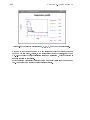
Click now the button Start/Continue in the dialog box Simulation to execute the
simulation. Plot the calculated results to the screen (by selecting the plot Conc and then
clicking the button Plot to Screen in the dialog box View Results). Fig. 3.4 shows
the resulting time courses of the concentrations CA , CB and CC . The concentration
CA decreases exponentially from its start value of 1 to zero. The concentration of the
48
CHAPTER 3. APPLICATION OF DATA ANALYSIS TECHNIQUES
Figure 3.4: Time course of the concentrations CA , CB and CC .
intermediate product CB increases from its start value of zero, reaches a maximum and
then decreases again to zero. The concentration of the end product CC raises to the
start value of 1 mg/l of substance A because the stoichiometric ratio of 0.5 from A to
B and of 2 from B to C lead to a stoichiometric factor of 1 for the combined reaction
from A to C .
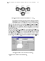
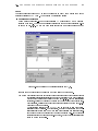
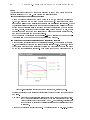
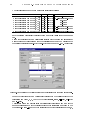
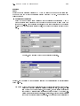
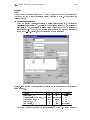
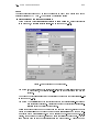
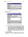
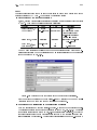
To dene and execute a sensitivity analysis click the command Calc!Sensitivity
Analysis from the main menu bar. This opens the dialog box shown in Fig. 3.5. A
denition of a sensitivity analysis consists of two parts: Active parameters must be
selected and one or more calculations must be dened. Selection of active parameters
is done with the two upper list boxes in this dialog box. Calculations can be dened by
clicking the button New between the two lower list boxes. This action opens the dialog
box already discussed in section 2.1 for dening calculations for simulations. Activate
now the parameters and calculations shown in Fig. 3.5.
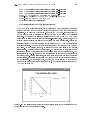
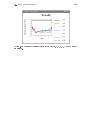
Click now the button Start in the dialog box shown in Fig. 3.5 to execute the sensitivity
analysis and specify a le name for the sensitivity ranking results. Now plot the
sensitivity functions by selecting each of the three plot denitions SensAR A, SensAR B
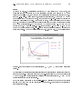
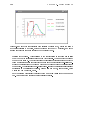
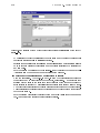
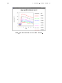
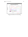
and SensAR C and clicking the button Plot to Screen. The Figs. 3.6, 3.7 and 3.8
show the result.
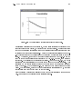
It becomes evident from Fig. 3.6 that A is insensitive to the parameters KB and rmax;B .
This is not astonishing as the rst process that only aects the concentration of A is
independent of these parameters. The dependence of A on the two parameters CA;ini
and kA is dierent: The sensitivity of CA with respect to CA;ini has its maximum at a
time of zero and decreases exponentially, while the sensitivity of CA with respect to kA
increases from zero, reaches a maximum and then decreases again to zero (this is the
behaviour of the absolute value of the sensitivity function; the negative sign indicates
that CA decreases with increasing values of kA ). This makes these two parameters
identiable from data of the concentration CA .
3.1. IDENTIFIABILITY ANALYSIS WITH SENSITIVITY FUNCTIONS
49
Figure 3.5: Denition of sensitivity analysis.
Fig. 3.7 shows that the dependence of CB on the parameters CA;ini and kA is dierent,
whereas the dependence of CB on the other two parameters KB and rmax;B leads to a
similar shape of the changes in CB , just with a dierent sign and magnitide. This means
that changes induced by changes in the parameter KB can be approximately balanced
by appropriate changes in the parameter rmax;B . This makes these two parameters
non-identiable from measured data of CB .
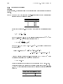
Since the sensitivity functions of CC shown in Fig. 3.8 lead to the same result (similar
behaviour of the sensitivity functions with respect to the parameters KB and rmax;B ),
also measured data of CC does not solve the identiability problem of the two parameters KB and rmax;B .
The reason of the non-identiability of the parameters KB and rmax;B is that the
concentrations CB are not much larger then the half-saturation concentration KB . In
this concentration range, the conversion rate of B to C can be linearized to rmax;B =KB CB , an expression which makes the non-identiability of KB and rmax;B evident.
Look also at the le specied after starting the sensitivity analysis. This le contains
a;r
a ranking of the time integral of the absolute values of the sensitivity functions y;p
and of the error contributions of all state variables with respect to all parameters in
all compartments (see the user manual for more details).
Save your system denitions by clicking the command File!Save from the main menu
bar. Answer No to the question to save calculated states.
50
CHAPTER 3. APPLICATION OF DATA ANALYSIS TECHNIQUES
Figure 3.6: Time course of the sensitivity functions of CA with respect to all four parameters.
3.1. IDENTIFIABILITY ANALYSIS WITH SENSITIVITY FUNCTIONS
51
Figure 3.7: Time course of the sensitivity functions of CB with respect to all four parameters.
52
CHAPTER 3. APPLICATION OF DATA ANALYSIS TECHNIQUES
Figure 3.8: Time course of the sensitivity functions of CC with respect to all four parameters.
3.1. IDENTIFIABILITY ANALYSIS WITH SENSITIVITY FUNCTIONS
53
Part B
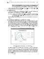
As shown in Fig. 3.7, the sensitivity function of CB with respect to KB and rmax;B are
of similar shape. The maximum of the sensitivity function with respect to KB has a
value of about 0:15 mg/l, the minimum of the sensitivity function with respect to rmax;B
is about ,0:2 mg/l. This means that, in linear approximation, a change in KB can be
compensated for by a change in rmax;B that is a factor of 0.15/0.2 as large (because the
result is more sensitive to rmax;B , the change in rmax;B must be smaller than the change
in KB ). The signs of the changes in the parameters must be the same because the changes
in CB have a dierent sign. If KB is changed by a factor of 2 from 0:5 mg/l to 1 mg/l a
change of rmax;B by a factor of 2 0:15=0:2, this means from 0:25 mg/l/h to 0:375 mg/l/h
would be the appropriate change. Fig. 3.9 shows the simulations performed for these new
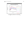
parameter values. The good correspondence of Fig. 3.9 with Fig. 3.4 demonstrates that
Figure 3.9: Time course of the concentrations CA , CB and CC for changed parameter
values.
the calculated concentrations for all substances are not signicantly dierent for these two
sets of parameters. This again conrms the non-identiability of the model parameters
KB and rmax;B from concentration time series of the three substances A, B and C in the
concentration range of this simulation.
Save your system denitions to the le sens b.aqu by clicking the command File!Save
As from the main menu bar and specifying the le name. Answer No to the question to
save calculated states.
54
CHAPTER 3. APPLICATION OF DATA ANALYSIS TECHNIQUES
3.2 Parameter Estimation
Problem
This example demonstrates how to use AQUASIM for performing parameter estimations
for a given model and given measured data. The example starts with a simple problem
of the estimation of parameters of rate expressions, it demonstrates how to include initial
conditions into the estimation process and it ends with the simultaneous estimation of
universal and experiment-specic parameters using the data of several experiments. The
identiability of the parameters is discussed using sensitivity functions and estimated
standard errors and correlation coecients. The approximative calculation of the standard
errors of model predictions and of the contributions of dierent parameters to the total
error is also discussed.
Part A: Use the measured time series on the le parest1.dat (Fig. 3.10) of decreasing
substrate concentration in a batch reactor with a volume of 10 l to estimate
the parameters half-saturation concentration K and maximum conversion rate
rmax of a Monod-type degradation process
dC = , rmax C
dt
K +C :
Start the calculation with the measured concentration at time zero. The data
series on the le parest1.dat is given in the units of h and mg/l (argument and
value in the rst and second column, respectively, data starting in row 4; see
Fig. 3.10). Use a relative standard deviation of 3% and an absolute standard
deviation of 0:1 mg/l. Use start values of K = 2 mg/l and rmax = 2 mg/l/h.
Compare rst a simulation using these parameter values with the measured
data, then perform a parameter estimation and compare the simulation based
on the estimated model parameter values with the measured data. Try to assess
the identiability of the model parameters with the aid of sensitivity functions
and estimated standard errors and correlation coecients.
Part B: In part A, the measurement inaccuracy of the initial concentration was ignored.
In order to apply a more convincing parameter estimation procedure treat now
the initial concentration as an additional parameter to be estimated by the program. Check again the sensitivity functions and the estimated standard errors
and correlation coecients for assessing the identiability of the (extended) set
of model parameters. Plot a model prediction with standard errors and the
contributions of all model parameters to the total error. Discuss the dierences
between the absolute-relative sensitivity functions and the error contributions.
Part C: Use the data from a second experiment with the same bacterial population
but with a dierent initial substrate concentration to increase the condence
in the estimated degradation rate parameters. The data series is given on the
le parest2.dat in the units h and mg/l (argument and value in the rst and
second column, respectively, data starting in row 4; see Fig. 3.10). Use a relative standard deviation of 3% and an absolute standard deviation of 0:02 mg/l.
Try again to assess the identiability of the model parameters with the aid of
sensitivity functions and estimated standard errors and correlation coecients.
3.2. PARAMETER ESTIMATION
Figure 3.10: Data sets 1 and 2 used for parameter estimation.
55
CHAPTER 3. APPLICATION OF DATA ANALYSIS TECHNIQUES
56
Solution
Part A
Start the window interface version of AQUASIM or click the command File!New from
the main menu bar to remove previously entered data from memory. Then perform the
following steps:
Denition of variables
Dene a state variable C for the concentration C of the substrate, a program variable
t referring to Time, and two constant variables K and rmax for the rate parameters
K and rmax with values of 2 mg/l and 2 mg/l/h, standard deviations of 0:2 mg/l
and 0:2 mg/l/h, minima of 0:01 mg/l and 0:01 mg/l/h and maxima of 10 mg/l and
10 mg/l/h.
Comment: The standard deviations of the constant variables are only used for sensitivity analyses. If a parameteter estimation is successful in estimating values and covariance
matrix of the parameters, the calculated standard deviation overwrites the value
specied here. For this reason, and because in the present example a parameter
estimation is performed before executing a sensitivity analysis, the value entered
for the standard deviation is irrelevant.
Dene a real list variable Cmeas with the argument t, a relative standard deviation of
0.03 and an absolute standard deviation of 0:1 mg/l and read the data pairs from the
le parest1.dat (argument and value in the rst and second colum, respectively, data
starting in row 4).
Denition of process
Dene a dynamic process Degradation as shown in Fig. 3.11.
Figure 3.11: Denition the process Degradation.
Denition of compartment
Dene a mixed reactor compartment Reactor with a volume of 10 l, activate the
variable C and the process Degradation and dene the variable Cmeas to be the initial
condition for the variable C.
3.2. PARAMETER ESTIMATION
57
Denition of plots
Dene two plots Conc and Sens for concentrations and sensitivity functions. In the
rst plot dene two curves for the measured concentration Cmeas (Markers) and for
the calculated concentration C (solid line). In the second plot dene two curves for
the absolute-relative sensitivity functions of C with respect to the parameters K and
rmax.
Comment: Usually, the data used for curves in a plot consists of the calculated values of
the variable to be plotted at the points of time of simulation output (for plots of
time series) or at the spatial grid points of the compartment (for plots of spatial
proles). Lines are straight connections between these points, markers are plotted
at any of these points. There is one exception from this general rule: If the variable
to be plotted is a real list variable with the program variable Time as its argument
(for plots of time series) or with the program variable corresponding to the spatial
dimension of the compartment as its argument (for plots of spatial proles), then
the data points of the real list are used instead of the calculated values at points
of time of simulation output. This makes it possible to show measured data points
together with simulation results in the same plot.
If for such a real list the interpolated or smoothed values should be plotted, dene
a formula variable with the name of the real list variable as its algebraic expression
and plot this formula variable instead of or in addition to the real list. Then the
data points can be compared with the interpolated values.
Denition of simulation and parameter estimation
Figure 3.12: Denition of the t calculation.
Click the command Calc!Simulation from the main menu bar and dene a calculation of with 151 steps of 0.1 h. Select this calculation to be active for simulation as
well as active for sensitivity analysis. Click now the command Calc!Parameter
58
CHAPTER 3. APPLICATION OF DATA ANALYSIS TECHNIQUES
Estimation from the main menu bar and click the button New in the dialog box
Parameter Estimation. Dene the calculation for parameter estimation as shown in
Fig. 3.12. To add the t target, click the button Add, select the data set and specify
the variable, compartment, zone and spatial location for the comparison with the data
set as shown in Fig. 3.13.
Figure 3.13: Denition of the t target.
Comment: Note that in contrast to the denition of a calculation for simulation and/or sensitivity analysis (cf. Fig. 2.11), the denition of a calculation for parameter estimation shown in Fig. 3.12 does not require the specication of size and number of time
steps. This is not necessary, because the comparisons of calculation with measured
data takes place at given points in time at which the solution is calculated.
Note that several options in the dialog box Edit Fit Target shown in Fig. 3.13
are inactive. This is a consequence of the fact that the user has no choice if
there exists only one real list variable and only one compartment that consists
of one zone. The last entry of this dialog box Time/Space has the meaning of a
location in the compartment if the variable specied as Data is a time series, it
has the meaning of time, if the variable specied as Data is a spatial prole. In
the current case, this location is ignored because a mixed reactor compartment
does not resolve spatial coordinates.
Save your system denitions to the le parest a.aqu by clicking the command File!Save As from the main menu bar and specifying the le name.
Execution of simulation, parameter estimation and sensitivity analysis
In the dialog box Simulation (opened with Calc!Simulation) click the button
Start/Continue.
A plot of the simulation results (plot Conc), shown in Fig. 3.14,
demonstrates that the choice of the initial parameter values does not lead to a good
t.
In the dialog box Parameter Estimation (opened with Calc!Parameter Estimation),
activate the parameters K and rmax, select the Method to be secant and click the button Start to execute the parameter estimation.
Comment: The secant method converges much faster than the simplex method and it calculates estimates for the standard deviations and the correlation matrix in addition
to the estimates of the values of the parameters. However, if the start values of
the parameters are far from the optimum or in case of important inuence of the
3.2. PARAMETER ESTIMATION
59
Figure 3.14: Comparison of simulation with measured data before execution of the parameter estimation procedure.
parameter constraints (minima and maxima of the constant variables) the secant
algorithm may have problems to converge. In this case it is recommeded to use the
simplex algorithm rst and improve convergence with the secant algorithm later
on.
Now you have to specify the name of a le on which more information on the progress of
the iterative estimation process and statistical information on the estimates is written.
The dialog box shown in Fig. 3.15 summarises the results of the parameter estimation
procedure. 19 iterations were required in order to achieve convergence of the parameter
estimation algorithm. The value of the parameter K was decreased from 2 to 1.38,
that of rmax from 2 to 1.15. The deviation between model results and data decreased
from 1285 to 14.6. A restart of the parameter estimation process does not improve
this result.
Comment: The estimated standard errors and correlations of the parameters are not given
in the dialog box shown in Fig. 3.15. This information can be found on the le
specied after clicking the Start button of the parameter estimation (the standard
errors are also copied to the edit eld Std. Dev. of the constant variables used
as parameters to be estimated). In the current example, the estimated standard
error for K is 0.33 mg/l, that of rmax 0.06 mg/l/h.
It is always recommeded to restart the algorithm in order to check nal convergence. Changing the algorithm between secant and simplex may be helpful for
dicult parameter estimations.
To redo the simulation click rst the button Initialize in the dialog box Simulation
and then the button Start/Continue. Plot now again the concentration as a function
of time. As shown in Fig. 3.16 (and expected from the small nal value of 2 ), the t
is now much better.
Comment: During parameter estimations output is only calculated at points of time where
data points exist. For this reason, plotted results just after execution of a parame-
60
CHAPTER 3. APPLICATION OF DATA ANALYSIS TECHNIQUES
Figure 3.15: Dialog box summarising the results of the parameter estimation procedure.
ter estimation is poorly resolved if the data points are not densely distributed over
time. In such cases it is recommended to redo the simulation before the results are
plotted (this simulation automatically uses the estimated parameter values). This
leads then to a plot that uses the temporal resolution dened for the calculation
instead of the temporal resolution of the data. In the case of a poor temporal
distribution of data points, this leads to better results, if the resolution of the
calculation is reasonably dened.
If you use a text editor to look at the le written during parameter estimation, you
see that the estimated correlation matrix shows a large correlation of 0.97 between the
two parameters. The reason for this high correlation can be seen by looking at the
sensitivity functions of C with respect to the two parameters K and rmax. In order
to be able to plot these sensitivity functions click the command Calc!Sensitivity
Analysis, activate the parameters K and rmax, click the button Start to execute the
sensitivity analysis, and specify a le name for a ranking of sensitivities. To plot the
sensitivity functions select the plot Sens and then click the button Plot to Screen.
The plot shown in Fig. 3.17 shows that the sensitivity functions of C with respect to K
and rmax are approximately linearly dependent. This means that a change in C caused
by a change in one parameter can be compensated by an appropriate change in the
other parameter. This behaviour leads to the shape of the 2 -surface shown in Fig.
3.18 that has a very poorly dened minimum.
Save your system denitions by clicking the command File!Save from the main menu
bar. Answer No to the question to save calculated states.
3.2. PARAMETER ESTIMATION
61
Figure 3.16: Comparison of simulation with measured data after execution of the parameter estimation procedure.
62
CHAPTER 3. APPLICATION OF DATA ANALYSIS TECHNIQUES
Figure 3.17: Sensitivity functions of C with respect to K and rmax.
3.2. PARAMETER ESTIMATION
63
11
10
log(chi^2) [−]
9
8
7
6
5
4
3
2
0
0
1
0.5
2
1
3
4
1.5
5
K [mg/l]
2
rmax [mg/l/h]
Figure 3.18: log(2 ) surface for Monod-model.
CHAPTER 3. APPLICATION OF DATA ANALYSIS TECHNIQUES
64
Part B
Continue just after doing part A or load the le saved in part A from within the window
interface version of AQUASIM. Then perform the following steps:
Modications of the system denitions
Dene a constant variable Cini with a value of 12 mg/l, a standard deviation of
1:2 mg/l, a minimum of 0 mg/l and a maximum of 100 mg/l. Activate the check boxes
active for sensitivity analysis and active for parameter estimation. Change
the initial condition for variable C in the compartment Reactor from Cmeas to Cini and
extend the plot denition Sens to contain a curve for the sensitivity of C with respect
to Cini. Finally, duplicate the plot denition Sens, change the name to Err, for all
curves change the curve type from Sensitivity Function to Error Contribution,
and adapt the plot title and the ordinate label.
Save your system denitions to the le parest b.aqu by clicking the command File!Save As from the main menu bar and specifying the le name.
Execution of parameter estimation and sensitivity analysis
Redo the parameter estimation and the sensitivity analysis. The nal value of 2 is now
12.1, the correlation between K and rmax decreased slightly to 0.95. Figure 3.19 shows
the dierent behaviour of the sensitivity function of C with respect to Cini compared
to the two other sensitivity functions. This means that the new parameter Cini is
Figure 3.19: Sensitivity functions of C with respect to K, rmax and Cini.
identiable although there exists an identiability problem between the parameters K
and rmax.
Comment: Note that the parameter estimation done in part B is much better than that of
part A because it considers the inaccuracy of the rst measurement at time zero.
Although usually only the parameters K and rmax are of interest, their estimates
can be improved by including the initial condition as an additional parameter to
be estimated.
Plot now the calculated values (plot Conc). The result is shown in Fig. 3.20. Because
3.2. PARAMETER ESTIMATION
65
Figure 3.20: Model predition with estimated standard error bars.
a sensitivity analysis has been performed, dotted lines indicating deviations by one
standard error are now plotted, in addition to the expected result. This standard error
of the model predition is calculated based on the linear error propagation formula with
omission of the parameter correlations. A plot of the error contributions shown in Fig.
3.21 (plot Err) shows the contribution of the dierent model parameters to the total
error. By denition, the shapes of the error contributions shown in Fig. 3.21 are the
same as those of the sensitivity functions shown in Fig. 3.19. However, the magnitude
is dierent. The results can be interpreted as follows. As shown in Fig. 3.19, the model
results are much less sensitive to the parameter K than to the parameter rmax. This
results in a much larger standard error of the parameter K (the estimated standard
error of K is 0.35, that of rmax is 0.09, the values of both parameters are of order
unity). For this reason, although the model results are less sensitive to K, the error
contribution for K is about the same as that for rmax.
Save your system denitions by clicking the command File!Save from the main menu
bar. Answer No to the question to save calculated states.
66
CHAPTER 3. APPLICATION OF DATA ANALYSIS TECHNIQUES
Figure 3.21: Error contributions of C with respect to K, rmax and Cini.
3.2. PARAMETER ESTIMATION
67
Part C
Continue just after doing part B or load the le saved in part B from within the window
interface version of AQUASIM. Then perform the following steps:
Modication of the system denitions
Duplicate the variable Cini and rename the duplicate to Cini1. Repeat this procedure for the variable Cini2. Introduce the program variable calcnum referring to the
Calculation Number. Select the variable Cini and then click the button Edit Type.
Select the type Variable List Variable. Redene now Cini in the dialog box Edit
Variable List Variable as shown in Fig. 3.22. This makes the initial condition to
Figure 3.22: Redenition of
Cini.
depend on the calculation number (note that the argument of the variable list is the
calculation number). For a calculation number of 1, the initial condition Cini1 is used,
for a calculation number of 2, the initial condition Cini2 is used.
Comment: Note that this approach can also be applied to parameters in transformation processes and not only to initial conditions. This would be meaningful if some of
these parameters seem to depend on the experiment.
Rename now the variable Cmeas to Cmeas1 and introduce an additional real list variable
Cmeas2 containing the time series read from the le parest2.dat (argument and value
in the rst and second colum, respectively, data starting in row 4).
In the Edit Calculation dialog box, change the name Calculation to Calculation1
and change its calculation number to 1. Add an additional calculation Calculation2
with a calculation number of 2 and with 100 steps of size 0:1 h.
Similarly change the calculation number of the existing t calculation to 1 and add an
additional t calculation with calculation number 2 and with the new variable Cmeas2
68
CHAPTER 3. APPLICATION OF DATA ANALYSIS TECHNIQUES
as the t target to be compared with the calculated values of the variable C.
Finally, change the name of the plot denitions Conc, Sens and Err to Conc1, Sens1 and
Err1 and change the calculation numbers of their curves to 1. Use the variable Cini1
as the parameter for describing the eect of the initial concentration. Now duplicate
the plot denitions Conc1, Sens1 and Err1 to Conc2, Sens2 and Err2, change the
calculation numbers from 1 to 2 and the variable Cini1 to Cini2.
Save your system denitions to the le parest c.aqu by clicking the command File!Save As from the main menu bar and specifying the le name.
Execution of parameter estimation and sensitivity analysis
Redo the parameter estimation and the sensitivity analysis. The parameters K and
rmax are now estimated much more accurately and with a much smaller correlation
(The standard error of K decreased from 0.35 to 0.10 mg/l, that of rmax remained
at 0.09 mg/l/h and the correlation coecient of these two parameters from 0.95 to
0.85). The cause for this observation is illustrated with the sensitivity function shown
in Figs. 3.23 and 3.24. The sensitvity functions of C with respect to K and rmax
Figure 3.23: Sensitivity functions of C with respect to K, rmax and Cini for experiment 1.
are still approximately linearly dependent for each experiment. However, the changes
necessary for one parameter to compensate for the eect of a change in the other
parameter are dierent for the two experiments. For this reason the identiability
of these two parameters is strongly increased if two experiments with dierent initial
concentrations are evaluated simultaneously. This is a typical result which illustrates
the important capability of AQUASIM to estimate parameters simultaneously using
data from dierent experiments.
Save your system denitions by clicking the command File!Save from the main menu
bar. Answer No to the question to save calculated states.
3.2. PARAMETER ESTIMATION
69
Figure 3.24: Sensitivity functions of C with respect to K, rmax and Cini for experiment 2.
CHAPTER 3. APPLICATION OF DATA ANALYSIS TECHNIQUES
70
3.3 Model Structure Selection
Problem
This example demonstrates the use of AQUASIM for model structure selection. Because
the gain in decrease of 2 that can be achieved by an increase in model structure complexity is used as a model structure selection criterion, this example provides also a good
training in parameter estimation. In addition, due the parallel implementation of dierent
models using calculation numbers, it is also an additional example of the use of calculation
numbers.
Part A: Respiration measurement have been performed in a stirred and aerated reactor
which has no inow and in which degradation of a mixture of organic substrates
takes place. The question to be answered is whether the substrate mixture
can approximatively be described by one (aggregated) state variable with a
linear or a Monod type degradation rate or if two dierent (less aggregated)
state variables representing easily and slowly degradable organic matter must
be distinguished. The respiration data is shown in Figs. 3.25 and 3.26. It is
measured with a standard deviation of 0:1 mg/l/h and is available on the data
le msel.dat.
Respiration Data
OUR [ m g/ l/ h]
16
14
12
10
8
6
4
2
0
0
1
2
3
4
5
t [h]
Figure 3.25: Respiration data to be used for model structure selection.
An evaluation between the following proposed model structures should be performed:
Model 1:
The degradation process can be described as a rst order process of a single
state variable C1 :
dC1 = , 1 X C = ,k C = ,r
1 1
M1 ;1
dt
Y1 1
Model 2:
The degradation process can be described as a process with a single state variable C1 but saturation eects represented by a Monod-type degradation rate
3.3. MODEL STRUCTURE SELECTION
71
Figure 3.26: Respiration data to be used for model structure selection.
are important:
dC1 = , 1 X C1 = , rmax;1 C1 = ,r
M2 ;1
dt
Y1 K1 + C1
K1 + C1
Model 3:
Two state variables C1 and C2 must be distinguished which represent fast and
slowly degradable organic components. The degradation of both components
can be described by a rst order process, however dierent rate constants must
be considered:
dC1 = , 1 X C = ,k C = ,r
1 1
M3 ;1
dt
Y1 1
dC2 = , 2 X C = ,k C = ,r
2 2
M3 ;2
dt
Y2 2
72
CHAPTER 3. APPLICATION OF DATA ANALYSIS TECHNIQUES
Model 4:
Two state variables C1 and C2 must be distinguished which represent fast and
slowly degradable organic components. The degradation of one of these components can be described by a rst order process, the degradation of the other
component must be described with a Monod-type process:
dC1 = , 1 X C = ,k C = ,r
1 1
M4 ;1
dt
Y1 1
dC1 = , 2 X C2 = , rmax;2 C2 = ,r
M4 ;2
dt
Y2 K2 + C2
K2 + C2
Model 5:
Two state variables C1 and C2 must be distinguished which represent fast and
slowly degradable organic components. The degradation of both components
must be described by Monod-type processes with dierent rate constants:
dC1 = , 1 X C1 = , rmax;1 C1 = ,r
M5 ;1
dt
Y1 K1 + C1
K1 + C1
dC1 = , 2 X C2 = , rmax;2 C2 = ,r
M5 ;2
dt
Y2 K2 + C2
K2 + C2
For all models, the oxygen uptake rate OUR which must be compared with the
measured data is given as
OURM =
i
2
X
j =1
(1 , Yi )rM ;j
i
where Yi is the yield of the process i.
Use a yield of Y = 0:67 (for all substrates) and perform parameter estimations
of the initial concentrations of the substrates and the model parameters for all
models. Then discuss which model is the most adequate for the description of
the data.
Part B: Discuss the dependence of the model structure selection process done in part A
on the value of the yield Y . Check your result by redoing some of the parameter
estimations with a yield of Y = 0:55.
3.3. MODEL STRUCTURE SELECTION
73
Solution
Part A
In order to evaluate all model structures the models could be implemented one after the
other by making appropriate changes to the process rates. This has the disadvantage
that it needs considerable editing for switching between model structures. For this reason
an alternative approach is described here that requires more eort in the rst implementation, but allows very fast switching between model structures once all structures have
been implemented. The program variable Calculation Number is used in order to switch
between model structures. Because in the current context a simultaneous t of the dierent models is not meaningful, any other variable could be used as an indicator of which
model should be used. The use of the calculation number makes switching between model
structures possible without changing the value of a variable.
Start the window interface version of AQUASIM or click the command File!New from
the main menu bar to remove previously entered data from memory. Then perform the
following steps:
Denition of variables
Dene two dynamic volume state variables C1 and C2 for the concentrations C1 and
C2 of the organic components.
Then dene the following model parameters as constant variables:
Meaning
Name
Unit Value Min. Max. St.Dev.
C1;ini for model 1 M1 C1ini mg/l
1
0
100
0.1
k1 for model 1
M1 k1
1/h
1
0
100
0.1
C1;ini for model 2 M2 C1ini mg/l
1
0
100
0.1
K1 for model 2
M2 K1
mg/l
1
0.1 100
0.1
rmax;1 for model 2 M2 rmax1 mg/l/h 1
0
100
0.1
C1;ini for model 3 M3 C1ini mg/l
1
0
100
0.1
C2;ini for model 3 M3 C2ini mg/l
1
0
100
0.1
k1 for model 3
M3 k1
1/h
1
0
100
0.1
k2 for model 3
M3 k2
1/h
1
0
100
0.1
C1;ini for model 4 M4 C1ini mg/l
1
0
100
0.1
C2;ini for model 4 M4 C2ini mg/l
1
0
100
0.1
k1 for model 4
M4 k1
1/h
1
0
100
0.1
K2 for model 4
M4 K2
mg/l
1
0.1 100
0.1
rmax;2 for model 4 M4 rmax2 mg/l/h 1
0
100
0.1
C1;ini for model 5 M5 C1ini mg/l
1
0
100
0.1
1
0
100
0.1
C2;ini for model 5 M5 C2ini mg/l
K1 for model 5
M5 K1
mg/l
1
0.1 100
0.1
K2 for model 5
M5 K2
mg/l
1
0.1 100
0.1
rmax;1 for model 5 M5 rmax1 mg/l/h 1
0
100
0.1
rmax;2 for model 5 M5 rmax2 mg/l/h 1
0
100
0.1
Save your system denitions to the le modsel a.aqu by clicking the command File!Save As from the main menu bar and specifying the le name.
Dene the variable calcnum as the program variable Calculation Number and the
variable zero as a formula variable with the value 0.
Comment: The variable zero is for use in a variable list variable, where it is not possible to
enter the value 0.
74
CHAPTER 3. APPLICATION OF DATA ANALYSIS TECHNIQUES
The process rates are now dened as formula variables as follows:
Meaning
Name
Rate for substrate 1 in model 1, rM1 ;1 r1 M1
Rate for substrate 1 in model 2, rM2 ;1 r1 M2
Rate for substrate 1 in model 3, rM3 ;1 r1 M3
Rate for substrate 2 in model 3, rM3 ;2 r2 M3
Rate for substrate 1 in model 4, rM4 ;1 r1 M4
Rate for substrate 2 in model 4, rM4 ;2 r2 M4
Rate for substrate 1 in model 5, rM5 ;1 r1 M5
Rate for substrate 2 in model 5, rM5 ;2 r2 M5
Unit
mg/l/h
mg/l/h
mg/l/h
mg/l/h
mg/l/h
mg/l/h
mg/l/h
mg/l/h
Expression
M1 k1*C1
M2 rmax1*C1/(M2
M3 k1*C1
M3 k2*C2
M4 k1*C1
M4 rmax2*C2/(M4
M5 rmax1*C1/(M5
M5 rmax2*C2/(M5
K1+C1)
K2+C2)
K1+C1)
K2+C2)
Save your system denitions by clicking the command File!Save from the main menu
bar.
Dene the variable C1ini as a variable list variable with the argument calcnum and
a list of argument value pairs so that the calculation numbers 1 to 5 correspond to
the initial concentrations M1 C1ini to M5 C1ini as shown in Fig. 3.27. Analogously
Figure 3.27: Denition of the variable C1ini as a variable list with the argument calcnum.
dene the variable C2ini as a variable list variable with the correspondence of the
calculation numbers 1, 2, 3, 4 and 5 to the variables zero, zero, M3 C2ini, M4 C2ini
and M5 C2ini.
Analogously dene the process rates as variable list variables r1 and r2 with the
argument calcnum and with the correspondence of the calculation numbers 1 to 5 to
the rates r1 M1 to r1 M5, and with the correspondence of the calculation numbers 1, 2,
3.3. MODEL STRUCTURE SELECTION
75
3, 4 and 5 to the rates zero, zero, r2 M3, r2 M4 and r2 M5, respectively. Figure 3.28
shows the denition of the variable r2.
Figure 3.28: Denition of the variable r2 as a variable list with the argument calcnum.
Save your system denitions by clicking the command File!Save from the main menu
bar.
Dene the variable t as the program variable time and the formula variable Y with a
value of 0.67 as the yield Y .
Now the calculated oxygen uptake rate can be dened as a formula variable resp calc
with the algebraic expression (1-Y)*(r1+r2) and the measured oxygen uptake rate as
a real list variable resp meas with the argument t, a standard deviation of 0:5 mg/l/h
and the 26 data pairs read from the le msel.dat.
Comment: This relatively large set of variables is necessary in order to be able to distinguish
the parameters of the dierent models. This is not in any case necessary, but
often recommendable because it allows the user to easily switch back to a model
of which the parameters were estimated earlier without the necessity to enter the
parameter values obtained form the earlier parameter estimation.
Save your system denitions by clicking the command File!Save from the main menu
bar.
Denition of processes
Dene two dynamic processes Degrad1 and Degrad2 with process rates r1 and r2 and
with a single stoichiometric coecient of ,1 for the substrates C1 and C2, respectively.
As an example, Fig. 3.29 shows the denition of the process Degrad1.
Denition of compartment
Dene a mixed reactor compartment reactor with a volume of 1. In this compartment
76
CHAPTER 3. APPLICATION OF DATA ANALYSIS TECHNIQUES
Figure 3.29: Denition the process Degrad1.
activate the state variables C1 and C2 and the processes Degrad1 and Degrad2. Finally,
specify C1ini and C2ini to be the initial concentrations of C1 and C2, respectively.
Denition of plot
Dene a plot with one curve consisting of markers for the variable resp meas and
ve curves with lines of dierent styles for the variable resp calc for the calculation
numbers 1 to 5.
Comment: The calculation number for the variable resp meas is irrelevant because in a plot
with abscissa time for a real list variable with the program variable Time as the
argument, the data pairs of the real list variable are plotted instead of interpolated
calculated values (if not desired, this feature can be omitted by plotting a formula
variable of which the algebraic expression consists of the name of the real list
variable).
Save your system denitions by clicking the command File!Save from the main menu
bar.
Denition of simulations and parameter estimations
Dene ve calculations with 250 steps of size 0.02 h and calculation numbers of 1, 2, 3,
4 and 5. Dene ve parameter estimation calculations Fit1 to Fit5 as shown in Fig.
3.30 for the example of Fit4 with the single t target of comparing the data stored
in the variable resp meas with the variable resp calc evaluated in the compartment
reactor and with use of the calculation numbers 1 to 5.
Save your system denitions by clicking the command File!Save from the main menu
bar.
Execution of parameter estimations
In the dialog box Parameter Estimation select the parameters M1 C1ini and M1 k1
and the calculation Fit1 to be active. Then click the button Start and specify the
name of a t le for storing details of the parameter estimation. The program nds a
nal value of 2 of about 142.1. A restart of the t algorithm by clicking the button
3.3. MODEL STRUCTURE SELECTION
77
Figure 3.30: Denition the t calculation Fit4.
Start
again does not improve the t.
Comment: It is always advisable to restart a t in order to check if nal convergence was
obtained. In case of bad convergece of the algorithm this may improve the result.
Figure 3.31 shows the results of this t. Obviously there are systematic deviations
between data and simulation. The sign of the curvature of the simulation is always the
same whereas it changes for the data.
Inactivate the parameters and the t calculation for model 1 and activate the parameters M2 C1ini, M2 K1 and M2 rmax1 and the calculation Fit2 for model 2. Performing
the parameter estimation leads to a 2 value of 67.8 that is slightly improved to 67.3 by
restarting the parameter estimation. Figure 3.32 shows the results of this t. Obviously
the t is signicantly improved, however, there are still systematic deviations between
measurements and the simulation, especially close to the end of the simulation.
Inactivate the parameters and the t calculation for model 2 and activate the parameters M3 C1ini, M3 C2ini, M3 k1 and M3 k2 and the calculation Fit3 for model 3. For
this model the parameter estimation process converges very badly and the minimum
of 2 is obtained only after several restarts of the parameter estimation. The solution
agrees with the solution of model 1 shown in Fig. 3.31 (the initial condition and the
degradation rate of the substrate C2 are set to zero). The algorithm obviously cannot
distinguish two exponential time scales.
Inactivate the parameters and the t calculation for model 3 and activate the parameters M4 C1ini, M4 C2ini, M4 k1, M4 K2 and M4 rmax2 and the calculation Fit4 for
model 4. The parameter estimation stops now at a value of 2 of 14.0 which is not
78
CHAPTER 3. APPLICATION OF DATA ANALYSIS TECHNIQUES
Figure 3.31: Comparison of the results of model 1 with the measurements.
improved upon restart of the algorithm. Figure 3.33 shows the results of this t. There
is excellent agreement of the simulation with the data.
Inactivate the parameters and the t calculation for model 4 and activate the parameters M5 C1ini, M5 C2ini, M5 K1, M5 K2, M5 rmax1 and M5 rmax2 and the calculation
Fit5 for model 5. Again, there is very bad convergence and the minimum of 2 of
14.0 is achieved only after several restarts of the parameter estimation algorithm. The
result cannot be distinguished from that of model 4 shown in Fig. 3.33.
The results can be summarised in the following table:
model no. of parameters
1
2
2
3
3
4
4
5
5
6
2
142.1
67.3
142.1
14.0
14.0
The model 4 is the rst model that does not lead to systematic deviations between
model results and data. It is obvious, that the increase in complexity from model 4
to model 5 does not reduce the value of 2 . For this reason, model 4 seems to be the
most adequate model that should be selected.
Save your system denitions by clicking the command File!Save from the main menu
bar. Answer No to the question to save calculated states.
3.3. MODEL STRUCTURE SELECTION
Figure 3.32: Comparison of the results of model 2 with the measurements.
79
80
CHAPTER 3. APPLICATION OF DATA ANALYSIS TECHNIQUES
Figure 3.33: Comparison of the results of model 4 with the measurements.
3.3. MODEL STRUCTURE SELECTION
Part B
81
It is obvious that a change in the value of Y only leads to a rescaling of the concentrations Ci (combined with a rescaling or the half-saturation concentrations Ki and of the
maximum conversion rates rmax;i ). The values of 2 are not aected by this rescaling and
therefore the model structure selection process leads to the same results. This can easily
be veried by setting the parameter Y in the AQUASIM system le created in part A to
a new value and redoing the parameter estimations.
82
CHAPTER 3. APPLICATION OF DATA ANALYSIS TECHNIQUES
Chapter 4
Numerical Parameters
Although AQUASIM uses the very robust and stiy stable integration algorithm DASSL
(Petzold, 1983), due to the exibility of the program which allows users to dene very
complicated models, numerical problems can occur during the time integration process.
In this chapter the most important types of numerical problems are shown. The goal of the
examples of this chapter is that AQUASIM users can learn a strategy of how to nd the
cause of numerical problems and how to solve them. For this reason, it is recommended
to invest some time for studying the examples of this chapter.
In the example discussed in section 4.1 problems of time integration and related numerical parameters are discussed. This example uses a simple model with a mixed reactor
compartment.
In the example discussed in section 4.2 problems of spatial discretization and related
numerical parameters are discussed. This example uses an advective-diusive reactor
compartment. The tutorial example for this compartment is given in section 5.2. However,
it should be possible to understand the example of section 4.2 without having studied the
example in section 5.2 before.
83
CHAPTER 4. NUMERICAL PARAMETERS
84
4.1 Parameters for Discretization in Time
Problem
This example demonstrates possible problems of numerical time integration and the meaning of numerical parameters.
Part A: In a stirred reactor with a volume of 1 l and a constant throughow of Q = 1
l/h a substance is added to the inow periodically at a concentration of 100
mg/l during the rst 0.01 h of any hour. The initial concentration is zero.
Calculate the concentration in the reactor as a function of time for 10 hours
(1000 steps of size 0.01 h) using the default values of all numerical parameters.
Plot the concentration time series and try to nd out the cause of the wrong
result. Then change the appropriate numerical parameter of the integration
algorithm, redo the simulation, and plot the correct result.
Part B: Add a relaxation process by starting the simulation 10 hours earlier with one
step of 10 hours followed by the simulation calculated above.
Try to nd the solution to the numerical problem during calculation.
Part C: Set the water and substance inows to zero and the initial concentration to 1
mg/l. Then add a degradation process with a rate of
p
r=k C
p
where C is the substance concentration and k = 1 mg/l/h is a rate constant.
Redo the simulation of part A (1000 steps of 0.01 h) and try to nd the cause
of the numerical problem during calculation. Change the process rate to an
expression that avoids the problem.
4.1. PARAMETERS FOR DISCRETIZATION IN TIME
85
Solution
Part A
Start the window interface version of AQUASIM or click the command File!New from
the main menu bar to remove previously entered data from memory. Then perform the
following steps:
Denition of variables
Dene a dynamic volume state variable C, a program variable t referring to Time, a
formula variable period with a value of 1 h, and a formula variable Qin with a value
of 1 l/s. Then dene the time within each period as a formula variable t period as
shown in Fig. 4.1. Now dene a real list variable Cin as shown in Fig. 4.2.
Figure 4.1: Denition of the time in hours within each period.
Comment: The modulo function easily allows to dene periodic functions as shown in Figs.
4.1 and 4.2 (cf. also part C of the example discussed in section 2.2). First the
time within each period is dened as shown in Fig. 4.1. Then this time is used as
an argument of a function implemented as a formula variable, a real list variable
or a variable list variable (cf. Fig. 4.2). In this way, the function automatically
becomes periodic.
Note that the input pulse is approximated by a continuous function the value of
which increases and decreases within a time interval of 0.001 h. This is necessary
because the integration algorithm has problems to step over discontinuities (if
necessary, the time interval for increase and decrease can be made shorter). Note
that the value of the real list variable at zero is the same as the value at the end
of the period (in this case the value at 0.011 is used for values of the argument
larger than 0.011). This is necessary to avoid a discontinuity when the argument
t period discontinuously switches back from the value after one period to zero.
Denition of compartment
Dene now a mixed reactor compartment with the variable C as an active state variable
with a water inow equal to Qin, with a substance input loading for the variable C of
Qin*Cin and with a constant volume of 1 (l).
Denition of plot
Dene a plot with abscissa time with a curve for the value of the variable C.
Denition of simulation
Dene an active calculation of 1000 steps of size 0.01 h.
Save your system denitions to the le numtim a.aqu by clicking the command File!Save As from the main menu bar and specifying the le name.
86
CHAPTER 4. NUMERICAL PARAMETERS
Figure 4.2: Denition of the periodic inow concentration as function of the time within
each period.
Execution of simulation and presentation of results
Figure 4.3 shows the results of the simulation. Within the rst 0.01 h the concentration
in the reactor increases as a consequence of the inow denition (rst pulse). Then
the concentration decreases exponentially due to the throughow through the reactor.
This behaviour is correct during the rst hour. But at the beginning of the second
hour, this is no longer correct. The next pulse of the periodic input signal should
lead to an increase in concentration similar to the increase at the beginning of the
simulation. Similarly all succeeding input pulses are ignored.
What is the cause of this error?
The integration algorithm selects its internal time step according to the accuracy requirements of the calculated concentration. At the beginning of the simulation it starts
with a very small time step. It then follows the input pulse and begins to increase the
step size during the rest of the rst hour, because the exponential decrease in concentration caused by the throughow can be calculated accurately also for relatively large
time steps. Because the time step at the end of the rst hour is much larger than the
pulse width of 0.01 h, the algorithm steps over the pulse. The same happens with all
succeeding pulses. If by chance the end of an integration time step would be within
an input pulse interval, the algorithm would recognise the problem (because the accuracy criterion fails for such a fast change in input concentration), the algorithm would
4.1. PARAMETERS FOR DISCRETIZATION IN TIME
87
Figure 4.3: Concentration time series with original values of numerical parameters. All
input pulses with exception of the rst are ignored by the program.
repeat the step by a sequence of smaller steps and it would follow this input pulse
accurately. However, in the present example, the chance for catching all input pulses
is very small because the integration of the exponential decrease in concentration is
very simple and, therefore, makes large integration time steps possible.
In order to avoid this problem, the internal step size of the integration algorithm
must be limited to a value smaller than the duration of the input pulses. If this is
done, at least one input evaluation is done within the pulse interval and therefore, as
explained above, the concentration time series of the pulse is followed accurately by the
integration algorithm. The internal step size of the integration algorithm can be limited
with the aid of the dialog box openend with the Numerical Parameters command of
the Edit menu. If the value of the numerical parameter Maximum Internal Step
Size in this dialog box is changed from 1 to 0.01 and the simulation is redone, the plot
shown in Fig. 4.4 results. This plot shows the correct behaviour of the concentration
in the reactor.
Save your system denitions by clicking the command File!Save from the main menu
bar. Answer No to the question to save calculated states.
88
CHAPTER 4. NUMERICAL PARAMETERS
Figure 4.4: Concentration time series with a value of 0.01 for the numerical parameter
Maximum Internal Step Size. All input pulses are considered correctly.
4.1. PARAMETERS FOR DISCRETIZATION IN TIME
89
Part B
Continue just after doing part A or load the le saved in part A from within the window
interface version of AQUASIM. Then perform the following steps:
Modication of the system denitions
Open the dialog box Simulation by clicking the command Simulation in the menu
Calc. Then open the dialog box Edit Calculation Definition by double-clicking
the name of your calculation. Modify the denition as shown in Fig. 4.5. The initial
Figure 4.5: Denition of a calculation with one step from -10 to 0 (no resolution of output
during time integration for relaxation) and 1000 steps from 0 to 10 (good resolution of
output during the interesting part of the simulation).
time must be changed to -10. To insert the calculation step from -10 to 0 select the
calculation step series used in part A (in order to add the new series before this series),
then write the numbers 10 and 1 in the dialog elds Step Size and Num. of Steps
below the list box of step series, and click the button Add.
Save your system denitions to the le numtim b.aqu by clicking the command File!Save As from the main menu bar and specifying the le name.
Execution of simulation and presentation of results
Now start the simulation. The simulation is interrupted with the message shown in
Fig. 4.6. On the log le, the following DASSL error message is printed:
90
CHAPTER 4. NUMERICAL PARAMETERS
Figure 4.6: Error message interrupting the dynamic simulation.
05/25/1998 17:51:30 Start of calculation
05/25/1998 17:51:30 Integration at time -10
DASSL{ AT CURRENT T = -4.51946 1000 STEPS
DASSL{ TAKEN ON THIS CALL BEFORE REACHING TOUT.
05/25/1998 17:51:30 End of calculation
*** Calculation stopped due to numerical problems ***
This error message indicates that the calculation was interrupted because the output
time was not reached within 1000 steps of the algorithm. This message may be a
hint for the presence of numerical problems, because the output resolution is usually
not adequate if so many steps are required for a single output step. In the present
case, the output step was chosen to be large because the dynamic behaviour during
the relaxation phase was not of interest. For this reason, it is no problem if more
than 1000 steps are required for one output step and the limit of 1000 steps should
be increased. This is done in the dialog box Edit Numerical Parameters which is
opened with the command Numerical Parameters in the menu Calc. In this dialog
box, increase the value of the parameter Maximum Number of Internal Time Steps
for one Output Time Step from 1000 to 10000. If now the simulation is redone,
no numerical problem occurs and the result looks as shown in Fig. 4.7. This gure
shows the correct result. Because the relaxation phase is done as one output time
step, the concentration is linearly interpolated between its values at -10 and at 0 h.
Then between 0 and 10 h the dynamics can be followed. By changing the scaling
of the plot, the relaxation phase can be eliminated from the plot. However, if the
dynamics of relaxation should be followed, more smaller output steps must be taken
during relaxation.
Save your system denitions by clicking the command File!Save from the main menu
bar. Answer No to the question to save calculated states.
4.1. PARAMETERS FOR DISCRETIZATION IN TIME
Figure 4.7: Concentration time series for relaxation and simulation.
91
CHAPTER 4. NUMERICAL PARAMETERS
92
Part C
Continue just after doing part B or load the le saved in part B from within the window
interface version of AQUASIM. Then perform the following steps:
Modication of the system denitionsp
Dene a formula variable k with a value of 1 mg/l/h and a dynamic process degradation with a rate of k*sqrt(C) and a stoichiometric coecient of -1 for the variable C.
Then, in the Edit Mixed Reactor Compartment dialog box, activate the new process,
add an initial condition of 1 mg/l for the variable C, set the inow to 0 and delete the
input ux for the variable C. Delete the relaxation time step of 10 h and set the initial
time to 0.
Save your system denitions to the le numtim c.aqu by clicking the command File!Save As from the main menu bar and specifying the le name.
Execution of simulation and presentation of results
Now start the simulation. The simulation is interrupted with a message of a numerical
problem (cf. Fig. 4.6). The simulation result up to the interruption looks as shown
in Fig. 4.8. The result looks quite reasonable and gives no direct indication of the
Figure 4.8: Concentration time series up to the interruption by the numerical problem.
problem. The log le of the session contains the following messages:
05/25/1998 17:53:29 Integration at time 1.97
05/25/1998 17:53:29 Integration at time 1.98
05/25/1998 17:53:29 Integration at time 1.99
FORMVAR numerical problem: illegal value in variable rate degradation
FORMVAR numerical problem: illegal value in variable rate degradation
FORMVAR numerical problem: illegal value in variable rate degradation
FORMVAR numerical problem: illegal value in variable rate degradation
05/25/1998 17:53:29 Integration at time 2
FORMVAR numerical problem: illegal value in variable rate degradation
FORMVAR numerical problem: illegal value in variable rate degradation
FORMVAR numerical problem: illegal value in variable rate degradation
4.1. PARAMETERS FOR DISCRETIZATION IN TIME
93
FORMVAR numerical problem: illegal value in variable rate degradation
FORMVAR numerical problem: illegal value in variable rate degradation
FORMVAR numerical problem: illegal value in variable rate degradation
DASSL{ AT T = 2.00014 AND STEPSIZE H = 1.49012e-010
DASSL{ THE CORRECTOR COULD NOT CONVERGE BECAUSE
DASSL{ IRES WAS EQUAL TO MINUS ONE
05/25/1998 17:53:29 End of calculation
*** Calculation stopped due to numerical problems ***
The DASSL error message indicates, that the algorithm which calculates the solution
after one time step did not converge although the size of the time step was decreased
drastically. The cause (IRES equal to -1) is that the AQUASIM-function called by
DASSL was not able to calculate the right hand side of the system of dierential
equations. This cause can closer be localized with the aid of the AQUASIM error
messages on an illegal value in the variable rate degradation. Unfortunately, such a
variable does not exist in the list box of the dialog box Edit Variables. Besides the
variables entered by the user (and seen in this dialog box) AQUASIM uses additional
variables internally. The name of these variables should make clear to which quantity
they refer. In the present example, it refers to the edit eld Rate of the process
degradation. This rate is given as k*sqrt(C). An illegal value of this variable may
therefore be caused by an illegal value or a negative value of the concentration C. The
result plotted in Fig. 4.8 shows that the concentration at the time of the interrupt is
very close to zero. In such situations, also for models that would not lead to negative
concentrations, numerical inaccuracies may lead to (very small) negative values of
the concentration. In the present case, however, the model solution in fact becomes
undened (as a real number) at this point of time. The dierential equation solved by
AQUASIM is given as
Figure 4.9: Time series of the square root of the absolute value of the concentration up to
the interruption by the numerical problem.
CHAPTER 4. NUMERICAL PARAMETERS
94
dC = ,kpC :
dt
The analytical solution of this equation for an initial concentration C0 is
p
p
C (t) = C0 , kt2
:
p
The concentration, C , becomes complex for t > 2 C0 =k. For this reason, the calculation must run into numerical problems at t = 2 h. The problem can clearer be seen
if a new formula variable sqrtC is introduced as sqrt(abs(C)). A plot of the value of
this variable is shown in Fig. 4.9. It is evident, that the simulation runs into problems
at t = 2 h.
p
This problem makes it evident that the process rate k C is not a good
p process formulation, at least not for small concentrations. If the process rate k C is a good
description for reasonably large concentrations, the simplest correction to the process
rate could be to replace it by a linear process rate for concentrations below a critical
concentration Ccrit . In Fig. 4.10 it is shown how this can be done. Note that the
Figure 4.10: Dialog box showing the modied process rate denition.
proposed expression
8
<
r=:
p
k C
p
k Ccrit CC
crit
for C Ccrit
for C Ccrit
leads to equal results as the previous expression for concentrations larger than Ccrit , is
linear for concentrations smaller than Ccrit , and is continuous at Ccrit . A simulation
with this modied rate and with a value of Ccrit = 0:001 mg/l can be done without
any numerical problems. The result is shown in Fig. 4.11.
Save your system denitions by clicking the command File!Save from the main menu
bar. Answer No to the question to save calculated states.
4.1. PARAMETERS FOR DISCRETIZATION IN TIME
Figure 4.11: Concentration time series with the modied process rate denition.
95
96
CHAPTER 4. NUMERICAL PARAMETERS
4.2 Parameters for Discretization in Space
Problem
This example demonstrates possible problems in space discretization and the meaning
of numerical parameters. The example uses an advective-diusive reactor compartment.
The tutorial example for this compartment is given in section 5.2. However, it should be
possible to understand this example without having studied the example in section 5.2
before.
Part A: Calculate the advective transport of a concentration input pulse
2
(
t
,
t
0)
C1;in(t) = 10 mg/l exp , 22
with t0 = 1500 s and = 500 s through a 200 m long channel with a crosssectional area of 5 m2 and a discharge of 1 m3 /s. Implement the channel as
an advective-diusive reactor compartment without diusion and compare the
result with the analytical solution given as
2
(
t
,
t
0 , tadv )
C1;out (t) = 10 mg/l exp ,
22
with an advection time of tadv = 1000 s.
Use 52 grid points for spatial discretization, select the low resolution discretization technique and compare the numerical and with the analytical concentration
time series at the end of the channel after performing 400 output steps of 10 s.
Try to accelerate the calculation by increasing the numerical parameter Maximum
Internal Step Size and by decreasing the numerical parameter Number of
Codiagonals of the Jacobian Matrix (these parameters are accessible with
the command Edit!Numerical Parameters from the main menu bar).
Part B: Change now to the initial width from 500 s to 100 s and repeat the simulation
done in part A. Interpret the result.
Try to improve the the result by changing the number of grid points from 52 to
202 and/or by using the high resolution spatial discretization technique.
Try to reproduce the result of the simulation with 52 grid points and low resolution with 202 grid points and high resolution by introducing a diusion coecient with an appropriate value. Find this value by trial and error and compare
it with the value
L
Dnum 12 vx = 12 Q
A n,2
expected for numerical diusion (v is the advective velocity, x is the length
of a cell used for discretization, L is the channel length and n is the number of
grid points used for spatial discretization).
Part C: Add a second substance with an input pulse that increases linearly from 0 to
10 mg/l during the time from 1469 to 1471 s, remains at 10 mg/l until a time of
1529 s is reached and then decreases linearly to zero during the time from 1529
to 1531 s. Introduce again the analytical solution consisting of the same pulse
shifted by 1000 s in time. Use a Maximum Internal Step Size of 200 s, redo
4.2. PARAMETERS FOR DISCRETIZATION IN SPACE
97
the simulation and look also at the spatial proles of the substance at 1600 s,
1800 s, 2000 s, 2200 s and 2400 s.
Redo the simulation after inactivating the concentration of the rst substance.
Interpret your result and change the appropriate numerical parameter to obtain
the correct result.
Part D: Divide the advective-diusive reactor compartment in two advectively linked
advective-diusive compartments with the same total length, the same total
number of discretization cells and the same input at the inlet to the rst compartment. Distinguish the names of the compartments by appending ` 1' to the
original name for the rst compartment and by appending ` 2' to the original
name for the second compartment. Reproduce the nal simulation done in part
C.
Now, rename the compartments by replacing ` 1' by ` up' and ` 2' by ` down'.
Redo the simulation and try to nd out and x the numerical problem that
occurs.
CHAPTER 4. NUMERICAL PARAMETERS
98
Solution
Part A
Start the window interface version of AQUASIM or click the command File!New from
the main menu bar to remove previously entered data from memory. Then perform the
following steps:
Denition of variables
Dene a state variable C1, a program variable t referring to Time, and formula variables Qin, sigma, t0 and tadv with values of 1 m3 /s, 500 s, 1500 s and 1000 s, respectively. Then dene two formula variables C1in as 10*exp(-(t-t0)^2/(2*sigma^2))
and C1out as 10*exp(-(t-t0-tadv)^2/(2*sigma^2)).
Denition of compartment
Dene an advective-diusive reactor compartment PlugFlowReact and activate the
state variable C1. Click the button Input, then select the radio button Inlet Input
and dene the Water Inflow to be Qin and the Loading for the variable C1 to be
Qin*C1in as shown in Fig. 4.12. Then dene the Start Coordinate to be 0 (m),
Figure 4.12: Denition of the water and substance input to the compartment.
the End Coordinate to be 200 (m), and the Cross Sectional Area to be 5 (m2 ).
Select the radio button without diffusion, specify the Number of Grid Points to
be 52, and select the Resolution to be low. These denitions of the advective-diusive
reactor compartment are shown in Fig. 4.13.
Comment: Within the advective-diusive reactor compartment for all dynamic volume state
variables one-dimensional advection-diusion-reaction equations are solved (or pure
advection-reaction equations if in the dialog box shown in Fig. 4.13 the radio
button without diffusion is selected). These equations can describe advection, advection-diusion or advection-dispersion processes coupled with substance
transformations. The advective velocity is given as Q=A where Q is the discharge
and A the cross-sectional area. The discharge, Q, is equal to the Water Inflow
specied in the dialog box shown in Fig. 4.12 plus the outow of all advective
links connected to the inow of the compartment. The cross-sectional area, A,
is dened in the edit eld Cross. Sect. in the dialog box shown in Fig. 4.13.
With the aid of the program variable Space Coordinate X, the cross-sectional
4.2. PARAMETERS FOR DISCRETIZATION IN SPACE
99
Figure 4.13: Denition of the advective-diusive reactor compartment.
area may become dependent on the location along the compartment (an algebraic
expression can be entered in this edit eld or the cross-sectional area can be dened as a real list variable with the program variable Space Coordinate X as the
argument and this variable can be specied in the edit eld Cross. Sect.). The
numerical algorithm used for solving the advection-diusion equation requires a
user-specied discretization of the direction along the reactor that uses n , 2 cells
of equal length if n denotes the number of grid points selected in the dialog box
shown in Fig. 4.13 (two grid points are used for the start and end points of the
reactor; the step size of the discretization in time is selected automatically by the
time integration algorithm). Finally, the Resolution of the spatial discretization
must be selected in the dialog box shown in Fig. 4.13. The low resolution method
uses a simple rst order discretization technique that is robust but leads to considerable numerical diusion (as discussed in part B of this example), the high
resolution method uses a second order discretization technique with ux limiters
in order to avoid numerical oscillations of the solutions.
Denition of plot
Dene a plot C1 t containing two curves for the value of the variable C1 evaluated in
the compartment PlugFlowReact at the Space location 200 (m) and for the value of
the variable C1out.
Comment: Because the variable C1out has a global value it is irrelevant in which compartment
and at which location it is evaluated (if the location is within the legal range for
the compartment).
Denition of simulation
Dene an active calculation of 400 steps of 10 s.
Save your system denitions to the le numspa a.aqu by clicking the command File!Save As from the main menu bar and specifying the le name.
Execution of simulation and presentation of results
Start now the simulation and look at the results shown in Fig. 4.14. The numerical
solution shows reasonable agreement with the analytical solution. A small peak atten-
CHAPTER 4. NUMERICAL PARAMETERS
100
Figure 4.14: Comparison of the analytical and the numerical solution of part A.
uation occurs due to numerical diusion that will be discussed in more detail in part
B of this example.
The simulation speed can now be increased signicantly by changing the numerical
parameters as shown in Fig. 4.15. This dialog box is opend by clicking the command
Figure 4.15: Numerical parameters as used for speeding up the integration process.
!
Edit Numerical Parameters from the main menu bar. The
Internal Step Size has been increased from its default value of
rameter Number of Codiagonals of the Jacobian Matrix has
its default value 1000 to 8.
parameter Maximum
1 to 100 and the pabeen decreased from
Comment: The integration time step is selected (and changed) automatically by the numerical
integration algorithm (the solution is then interpolated at the points of time selected by the user with the external time step). The parameter Maximum Internal
Step Size sets an upper bound to the internal time step selected by the algorithm.
In the current example a maximum of 1 (s) leads to the execution of more time
steps then necessary for keeping the integration at a reasonable accuracy. There-
4.2. PARAMETERS FOR DISCRETIZATION IN SPACE
101
fore, an increase of this parameter speeds up the calculation.
The implicit numerical solver DASSL (Petzold, 1983) used for time integration of
the spatially discretized partial dierential equations (together with the ordinary
dierential equations and with the algebraic equations) requires the calculation
of the matrix of the partial derivatives of the right-hand sides of the dierential
equations with respect to the state variables (Jacobian matrix). If the spatial
conguration of the model implemented in AQUASIM does not contain recirculations, probe variables and biolm compartments and if the ow through the linear
arrangement of reactors is according to the alphabetical list in the dialog box
Edit Compartments, then this matrix is banded and a reduction of the number
of codiagonals of this matrix signicantly increases calculation speed. The lower
the number of state variables, the lower the number of necessary codiagonals. In
the current case, the limitation to 8 codiagonals leads to a signicant indrease in
calculation speed.
Save your system denitions by clicking the command File!Save from the main menu
bar. Answer No to the question to save calculated states.
CHAPTER 4. NUMERICAL PARAMETERS
102
Part B
Continue just after doing part A or load the le saved in part A from within the window
interface version of AQUASIM. Then perform the following steps:
Modication of the system denitions
Change the value of the variable sigma from 500 s to 100 s.
Save your system denitions to the le numspa b.aqu by clicking the command File!Save As from the main menu bar and specifying the le name.
Execution of simulation and presentation of results
Redo the simulation and plot the results. Fig. 4.16 shows the comparison of the
analytical with the numerical solution for this new value of . In contrast to the
Figure 4.16: Comparison of numerical and analytical solution for 52 grid points and low
resolution discretization.
simulation with = 500 s done in part A (Fig. 4.14) the numerical solution for =
100 s deviates signicantly from the analytical solution. This is due to numerical
diusion which has a larger eect to the narrower pulse in part B than it had in part
A.
Increase now in the dialog box Edit Advective-Diffusive Compartment shown in
Fig. 4.13 the number of grid points to 202, redo the simulation and plot the results.
The numerically calculated peak becomes now narrower, but there is still a signicant
deviation between the numerical and the analytical solution.
Switch now back to 52 grid points but select the high resolution discretization scheme.
The result is even better than for the simulation performed before with 202 grid points
and the low resolution scheme.
Finally, use 202 grid points and the high resolution scheme, redo the simulation and
plot the results. This result is shown in Fig. 4.17. For the current peak width, there is
now a good agreement between the numerical and the analytical solution. This means
that there is no signicant numerical diusion.
In the dialog box Edit Advective-Diffusive Compartment select now the radio but-
4.2. PARAMETERS FOR DISCRETIZATION IN SPACE
103
Figure 4.17: Comparison of numerical and analytical solution for 202 grid points and high
resolution discretization.
ton with diffusion and specify a diusion coecient. Redo the simulation and look
at the results. With a diusion coecient between 0:3 m2 /s and 0:6 m2 /s the numerical solution is similar to that for the simulation with 52 grid points and the low
resolution discretization. This result corresponds to a value of the numerical diusion
of Dnum = 0:4 m2 /s calculated with the formula given above (Dnum vx=2).
Comment: The occurrence of numerical diusion has the following consequences: If diusion
(or dispersion) is negligible in the system considered, the resolution of the discretization must be so high that for the puls widths typical in the system the eect
of numerical diusion can be neglected. The equation Dnum vx=2 valid for the
rst order (low resolution) discretization scheme may help nding the adequate resolution. If there is signicant diusion (or dispersion) in the investigated system,
there are two possibilities: The discretization can be chosen in such a way that the
numerical diusion can be neglected and the real diusion coecient is entered
as a diusion coecient in the dialog box used for editing the advective-diusive
reactor compartment, or a rst order (low resolution) discretization technique together with a purely advective compartment (option: without diffusion) can
be used with the number of grid points chosen such that the numerical diusion
is equal to the real diusion. From a conceptual point of view the rst technique
is more satisfying, however, from a pragmatic point of view the second technique
is appealing because the computational demand is minimised.
Save your system denitions by clicking the command File!Save from the main menu
bar. Answer No to the question to save calculated states.
CHAPTER 4. NUMERICAL PARAMETERS
104
Part C
Continue just after doing part B or load the le saved in part B from within the window
interface version of AQUASIM. Then perform the following steps:
Modication of the system denitions
Add a state variable C2 and two real list variables C2in and C2out as shown in the
Figs. 4.18 and 4.19.
Figure 4.18: Denition of the real list variable C2in.
Activate the variable C2 in the compartment PlugFlowReact and specify the Input
Flux for the variable C2 into this compartment as Qin*C2in.
Set the numerical parameter Maximum Internal Step Size to 200 (s).
Duplicate the plot denition C1 t, change the name to C2 t and change the variable
names from C1 to C2 and from C1out to C2out. Select the line style for the variable
C2out to be solid. Add an additional plot denition as shown in Fig. 4.20.
Save your system denitions to the le numspa c.aqu by clicking the command File!Save As from the main menu bar and specifying the le name.
Execution of simulation and presentation of results
Redo the simulation and look at the result shown as a time series in Fig. 4.21 and as
spatial proles in Fig. 4.22. Note that for extremely sharp pulses a small numerical
diusion eect can hardly be avoided.
Inactivate now the variable C1 in the compartment PlugFlowReact and redo simulation
and plot. The pulse has been disappeared! The reason for this problem is that now
4.2. PARAMETERS FOR DISCRETIZATION IN SPACE
105
Figure 4.19: Denition of the real list variable C2out.
the time step limiting rst substance is not longer calculated by the program. Because
the concentration of the second substance is constant (zero) during quite a long time,
the integration time step increases to its maximum of 200 s. With such a large time
step it is possible that the integration algorithm steps over the input pulse without
recognising the change in concentration. This problem can be solved by reducing the
Maximum Internal Step Size to 50 (s). With this step size, the integrator cannot
overstep an input pulse with a length of 60 s. If the integrator recognises the pulse,
the step size is automatically decreased in order to follow its shape accurately.
Save your system denitions by clicking the command File!Save from the main menu
bar. Answer No to the question to save calculated states.
106
CHAPTER 4. NUMERICAL PARAMETERS
Figure 4.20: Denition of the plot for spatial proles of C2.
4.2. PARAMETERS FOR DISCRETIZATION IN SPACE
Figure 4.21: Output times series of the variable C2.
107
108
CHAPTER 4. NUMERICAL PARAMETERS
Figure 4.22: Spatial proles of the variable C2.
4.2. PARAMETERS FOR DISCRETIZATION IN SPACE
109
Part D
Continue just after doing part C or load the le saved in part C from within the window
interface version of AQUASIM. Then perform the following steps:
Modication of the system denitions
Rename the compartment PlugFlowReact to PlugFlowReact 1, reduce the End Coordinate from 200 to 100 and reduce the Num. of Grid Points from 202 to 102 (this
corresponds to a reduction of the number of cells from 200 to 100). Then duplicate the
compartment. Change the name of the copied compartment from PlugFlowReact 1
to PlugFlowReact 2, the Start Coordinate from 0 to 100 and the End Coordinate
from 100 to 200. Then click the button Input, set the Water Inflow to 0 and delete
the inlet Loadings.
Dene an advective link from compartment PlugFlowReact 1 to compartment PlugFlowReact 2.
In the plot denition for the concentration time series change the compartment for the
evaluation of the curve at the location 200 m from PlugFlowReact 1 to PlugFlowReact 2.
Save your system denitions to the le numspa d.aqu by clicking the command File!Save As from the main menu bar and specifying the le name.
Execution of simulation and presentation of results
The simulation can now easily be redone and leads to the same results as in part C (in
order to look at the concentration proles, additional curves must be dened for the
same points of time in the compartment PlugFlowReact 2).
Rename now the compartment PlugFlowReact 1 to PlugFlowReact up and the compartment PlugFlowReact 2 to PlugFlowReact down and restart the simulation. The
initialization stops with a message of numerical problems.
What is the cause for these problems?
The partial dierential equations are discretized in space in the alphabetical order in
which they are listed in the dialog box Edit Compartments. If the alphabetical order
corresponds to the ow direction, in the discretization scheme, the last grid points of
the rst compartment are close to the rst grid points of the second compartment.
This means that the advective link connects neighbouring grid points. This leads to a
Jacobian matrix that is banded (within the compartments it is banded for the same
reason). For this reason, computation time can be saved by limiting the number of
codiagonals that are evaluated by the integration algorithm as it has been done in this
example. However, if renaming changes the order of the compartments, the advective
link that connects the last grid points of the upstream compartment with the rst
grid points of the downstream compartment connects the last grid points of the overall
set with the rst grid points. This leads to nonzero elements of the Jacobian matrix
far from the diagonal. For this reason, integration with this discretization scheme
does not converge if only a small number of codiagonals of the Jacobian matrix are
evaluated. If the value of the numerical parameter Number of Codiagonals of the
Jacobian Matrix in the dialog box opened by clicking the command Edit!Numerical
Parameters is increased to 1000 (any value larger than the number of ordinary differential equations to be solved after spatial discretization leads to the evaluation of
the full Jacobian matrix) the simulation runs without problems and the result is again
equal to that in part C. However, the evaluation of the full Jacobian matrix makes
110
CHAPTER 4. NUMERICAL PARAMETERS
the simulation signicantly slower. For this reason, it is important to try to guarantee
a banded Jacobian matrix if this is possible (recirculations always generate nonzero
elements of the Jacobian matrix far from the diagonal).
Chapter 5
Compartments
The basic AQUASIM features have been discussed in the chapters 2 to 4 using systems
consisting of mixed reactors (with the exception of section 4.2). The goal of this chapter
is to give an introduction to the various alternatives for more complicated compartments.
In section 5.1 a simple example for an application of the biolm reactor compartment
is discussed. This example demonstrates how substrate and population gradients over the
depth of a biolm can be modelled with AQUASIM.
The introduction of the advective-diusive reactor compartment in section 5.2 is used
to demonstrate the dierence between ux-averaged and volume-averaged concentrations.
This dierence often causes problems in understanding calculated concentration steps if
the diusion or dispersion coecient changes discontinuously.
In section 5.3 the soil column compartment is introduced. This is an extension of the
advective-diusive reactor compartment with respect to the consideration of diusion into
immobile regions.
Another extension of the advective-diusive reactor compartment, the river section
compartment, is discussed in section 5.4. In this compartment, instead of the continuity
equation for water ow within a given cross-sectional area, simplied versions of the openchannel ow equations are solved. The transport processes are described analogously to
the advective-diusive reactor compartment with a diusion-type approximation to the
dispersion process.
The last compartment describing stratication, transport and transformation processes
in a horizontally well-mixed lake is discussed in section 5.5.
In contrast to the chapters 2 to 4 which are very much recommended to be studied for
all AQUASIM users, in the present chapter, the user can select to study the examples for
the compartments in which he or she is interested.
111
112
CHAPTER 5. COMPARTMENTS
5.1 Biolm Reactor Compartment
The example of this section demonstrates how to calculate growth and structure of a
biolm on a substrate in a mixed reactor.
The main AQUASIM feature introduced in this section is the biolm reactor compartment.
Problem
Part A: Calculate growth and composition of a biolm which consists of two microbial
species. It is assumed that the volume of water owing over the biolm surface
area of 1 m2 is 10,3 m3 and remains constant. The water inow at a rate of
1 m3 /d contains two substrates at a concentrations of 10 gCOD/m3 each. The
density of both microorganisms is 25000 gCOD/m3 . Each microbial species
grows on one substrate only. Growth occurs with Monod-type rate laws with
maximum growth rates of 0.4 d,1 and 0.1 d,1 , half-saturation concentrations
of 5 gCOD/m3 and yield coecients of 0.01 and 0.5, respectively. Respiration
occurs with specic rates of 0.05 d,1 and 0.002 d,1 . The initial biolm thickness
is 10,4 m and the initial volume fractions of both species are 10 % (80 % of
the biolm consists of water). The diusion coecients of both substrates are
assumed to be 2 10,5 m2 /d.
Perform a simulation for 50 days and plot the concentration proles of the
dissolved substances and the volume fraction proles of the microorganisms at
the days 10, 25 and 50 and the biolm thickness as a function of time.
Part B: Assume a mass transfer resistance due to a molecular boundary layer of 10,4
m thickness at the biolm surface (diusivity of particles equal to 10,7 m2 /d)
and a detachment velocity equal to half of the growth velocity of the biolm.
Redo the simulation and discuss the dierences in the results.
5.1. BIOFILM REACTOR COMPARTMENT
113
Solution
Part A
Start the window interface version of AQUASIM or click the command File!New from
the main menu bar to remove previously entered data from memory. Then perform the
following steps:
Denition of variables
Dene a program variable LF referring to Biofilm Thickness as shown in Fig. 5.1.
Then dene dynamic volume state variables S1, S2, X1 and X2 for the two substrates
Figure 5.1: Denition of the biolm thickness as a program variable.
and the two microbial species, respectively. Then create the following formula variables:
Meaning
Name
Unit
Expression
Bacterial density, rho
gCOD/m^3
25000
Diusivity of S1, DS1
D S1
m^2/d
2e-5
Diusivity of S2, DS2
D S2
m^2/d
2e-5
Max. growth rate of X1, X1
mu X1
1/d
0.4
Max. growth rate of X2, X2
mu X2
1/d
0.1
Half-saturation conc. for S1, KS1 K S1 gCOD/m^3
5
Half-saturation conc. for S2, KS2 K S2 gCOD/m^3
5
Specic resp. rate of X1, bX1
b X1
1/d
0.05
Specic resp. rate of X2, bX2
b X2
1/d
0.002
eps X1
X1/rho
Volume fraction of X1, X1
Volume fraction of X2, X2
eps X2
X2/rho
Yield for growth of X1, YX1
Y X1
0.01
Yield for growth of X2, YX2
Y X2
0.5
Inow, Qin
Qin
m^3/d
1
Inow concentration of S1, S1;in S1in gCOD/m^3
10
Inow concentration of S2, S2;in S2in gCOD/m^3
10
Save your system denitions to the le film a.aqu by clicking the command File!Save As from the main menu bar and specifying the le name.
Denition of processes
Dene a dynamic process for growth of microbial species of type 1 as shown in Fig. 5.2.
By duplicating this process and replacing all S1 by S2, X1 by X2 and Y1 by Y2 create
the analogous process for microbial species of type 2. Then introduce a respiration
CHAPTER 5. COMPARTMENTS
114
Figure 5.2: Denition of the growth process of X1 with consumption of S1.
process Resp X1 with a rate of b X1*X1 and a stoichiometric coecient of -1 for X1.
Again add the analogous process for microbial species of type 2 by duplicating the
process Resp X1, renaming it to Resp X2 and replacing b X1 by b X2 and all X1 by X2.
Denition of compartment
Dene a biolm reactor compartment as shown in Fig. 5.3. Activate the state variables
S1, X1, S2 and X2 and the processes Gro X1, Gro X2, Resp X1 and Resp X2. Specify an
initial condition of 0.0001 for the variable LF in the zone Biofilm Matrix and initial
conditions of 0.1*rho for the variables X1 and X2 in the zone Biofilm Matrix. Then
specify the water inow to be Qin and input loadings of Qin*S1in and Qin*S2in for
the variables S1 and S2, respectively. Then dene particulate properties for the state
variable X1 by rst clicking the button Particulate Variables and then the button
Add. In the dialog box Edit Particulate Variable select the variable X1, specify
the Density to be equal to rho and set all other properties to zero. Do the same
for X2. Similarly, by clicking the button Dissolved Variables dene the Boundary
Layer Resistance to be zero and the Pore Diffusivity to be D S1 and D S2 for the
variables S1 and S2, respectively.
Save your system denitions by clicking the command File!Save from the main menu
bar.
Denition of plots
Dene a plot LF t with a curve for the lm thickness LF as a function of time. Then
dene a plot S z with proles of the substrate concentrations after 10, 25 and 50 d of
simulation. For each substrate and each point in time plot two curves: a line for the
zone Pore Water and a marker for the zone Bulk Volume.
Comment: In a plot of spatial proles, the bulk volume concentration is plotted as a point
at the biolm surface. If lines are plotted in the biolm matrix (or the pore
volume) and markers in the bulk volume, the discontinuity resulting from a surface
boundary layer can be made visible in the plot.
5.1. BIOFILM REACTOR COMPARTMENT
115
Figure 5.3: Denition of the biolm reactor compartment.
Finally, dene a plot X z with curves for both species in the biolm matrix after 10,
25 and 50 d of simulation.
Denition of the simulation
Dene an active calculation with 50 steps of 1 day.
Save your system denitions by clicking the command File!Save from the main menu
bar.
Execution of the simulation and presentation of results
The simulation is now started by clicking the button Start/Continue of the dialog box
Simulation. Then the results can be plotted. The Figs. 5.5 to 5.7 show the results.
The concentration of the substrate S1 which is consumed at a much higher rate than
S2 decreases much faster in the biolm. This makes growth of X1 only possible close
to the biolm surface. In the depth of the biolm X2 can grow on S2. The microbial
composition resulting from this behaviour is shown in Fig. 5.7.
Save your system denitions by clicking the command File!Save from the main menu
bar. Answer No to the question to save calculated states.
116
CHAPTER 5. COMPARTMENTS
Figure 5.4: Denition of plot for substrate proles.
5.1. BIOFILM REACTOR COMPARTMENT
Figure 5.5: Development of the biolm thickness as a function of time.
117
118
CHAPTER 5. COMPARTMENTS
Figure 5.6: Proles of both substrates at 10, 25 and 50 days.
5.1. BIOFILM REACTOR COMPARTMENT
119
Figure 5.7: Proles of the volume fractions of both microbial species at 10, 25 and 50
days.
CHAPTER 5. COMPARTMENTS
120
Part B
Continue just after doing part A or load the le saved in part A from within the window
interface version of AQUASIM. Then perform the following steps:
Modication of the system denitions
Dene a program variable uF referring to Growth Velocity of Biofilm, a formula
variable D X with a value of 1e-7 m2 /d, and a formula variable LL with a value of 0.0001
m. Then, for the particulate variables X1 and X2 add LL/D X as the Boundary Layer
Resistance and for the dissolved variables S1 and S2 add LL/D S1 and LL/D S2 as the
Boundary Layer Resistance, respectively. Figure 5.8 shows the example for S1 (this
dialog box is opened by clicking the button Dissolved Variables in the dialog box
Edit Biofilm Reactor Compartment).
Figure 5.8: Denition of the boundary layer resistance and the diusivity of a dissolved
variable.
Then add the expression if uF>0 then 0.5*uF else 0 endif as the global surface
detachment velocity in the dialog box Edit Biofilm Reactor Compartment as shown
in Fig. 5.9.
Comment: The formulation of the detachment velocity as given above guarantees that the detachment velocity does not become negative for shrinking biolms (the detachment
velocity must always be nonnegative).
Save your system denitions to the le film b.aqu by clicking the command File-
!Save As from the main menu bar and specifying the le name.
Execution of the simulation and presentation of results
The Figs. 5.10 and 5.11 show the calculated substrate and microorganism proles
for the new model. Biolm growth is smaller than in part A due to detachment and
smaller substrate ux into the lm.
Save your system denitions by clicking the command File!Save from the main menu
bar. Answer No to the question to save calculated states.
5.1. BIOFILM REACTOR COMPARTMENT
121
Figure 5.9: Denition of the biolm compartment; look in particular to the denition of
the surface detachment velocity.
122
CHAPTER 5. COMPARTMENTS
Figure 5.10: Proles of both substrates at 10, 25 and 50 days.
Figure 5.11: Proles of the volume fractions of both microbial species at 10, 25 and 50
days.
5.2. ADVECTIVE-DIFFUSIVE REACTOR COMPARTMENT
123
5.2 Advective-Diusive Reactor Compartment
The example of this section demonstrates how to calculate the transport of a substance
through an advective-diusive reactor.
The main AQUASIM feature introduced in this section is the advective-diusive reactor
compartment.
Problem
Part A: Calculate the break-through curve of a rectangular tracer pulse of the form
(arbitrary units)
time t inow concentration C
0.00
0
0.01
1
1.00
1
1.01
0
through a column with a cross-sectional area of 1 unit, a length of 1 unit, a
discharge of 1 unit, and a dispersion coecient of 0.1 units (arbitrary units).
Compare the inow concentration given above with the concentration time series
at the end of the column.
Part B: Dene a samling device with a volume of 0.01 units and link it advectively to
the outlet of the column. In addition to the concentration time series dened
above, plot the concentration time series at the start position of the column and
within the sampling device. Discuss the dierences in the plotted curves.
CHAPTER 5. COMPARTMENTS
124
Solution
Part A
Start the window interface version of AQUASIM or click the command File!New from
the main menu bar to remove previously entered data from memory. Then perform the
following steps:
Denition of variables
Dene a program variable t referring to Time. Dene a real list variable Cin for the
inow concentration as shown in Fig. 5.12. Dene a dynamic volume state variable C
Figure 5.12: Denition of the inow concentration as a function of time.
for the concentration of the tracer and two formula variables Qin with a value of 1 and
D with a value of 0.1.
Denition of compartment
Dene an advective-diusive reactor compartment as shown in Fig. 5.13. The large
number of grid points and the high resolution discretization technique were chosen in
order to avoid numerical diusion. Activate the variable C and dene an Inlet Input
with a Water Inflow equal to Qin and an Input Flux for the variable C equal to
Qin*Cin.
Denition of plot
Dene a plot with time series for Cin and for C evaluated at the location 1 (end of the
compartment) in the advective-diusive compartment.
5.2. ADVECTIVE-DIFFUSIVE REACTOR COMPARTMENT
125
Figure 5.13: Denition of the advective-diusive reactor compartment.
Denition of simulation
Dene an active calculation with 300 steps of size 0.01 and reduce the numerical parameter Number of Codiagonals of the Jacobian Matrix to 10.
Save your system denitions to the le advdif a.aqu by clicking the command File!Save As from the main menu bar and specifying the le name.
Execution of the simulation and presentation of results
Start the simulation and plot the results. These are shown in Fig. 5.14. The pulse is
Figure 5.14: Concentration time series in the inlet and in the column at the outlet position.
shifted in time and spreaded through the eect of dispersion or diusion.
126
CHAPTER 5. COMPARTMENTS
Save your system denitions by clicking the command File!Save from the main menu
bar. Answer No to the question to save calculated states.
5.2. ADVECTIVE-DIFFUSIVE REACTOR COMPARTMENT
127
Part B
Continue just after doing part A or load the le saved in part A from within the window
interface version of AQUASIM. Then perform the following steps:
Modication of the system denitions
Create a mixed reactor compartment sampler with a constant volume of 0.01 and
activate the variable C. Then create an advective link from the outlet of the advectivediusive reactor compartment column to the mixed reactor compartment sampler as
shown in Fig. 5.15. Finally add two curves to the existing plot denition for time series
Figure 5.15: Denition of the advective link from the column to the sampler.
of the variable C in the advective-diusive compartment at location 0 (start position of
the column) and of the same variable evaluated in the new mixed reactor compartment.
Save your system denitions to the le advdif b.aqu by clicking the command File!Save As from the main menu bar and specifying the le name.
Execution of the calculation and presentation of results
Redo the simulation. Figure 5.16 shows the results of the calculation. Note that the
concentration in the inlet is not identical to the concentration at the start position of
the column and the concentration in the sampler is not identical to the concentration
at the end of the column. The reason for this fact is that AQUASIM guarantees mass
conservation at the inlet and at the outlet and that the diusion coecient D changes
discontinuously between the compartments. Substance loading in the column is given
as the sum of advective and diusive or dispersive loadings as
I = QC , AD @C
@x
This expression cannot remain constant without changes in C or @C=@x if D changes
its value. For this reason, if mass conservation is guaranteed, a discontinuity in the
diusion coecient leads to a discontinuity in concentration. At the inlet, the loading is
specied as I = QCin . This means that dispersion and/or diusion is neglected in the
inlet. At the start position of the column, this loading is equal to the expression given
above with a nonzero diusion coecient and with the concentration prole at the start
128
CHAPTER 5. COMPARTMENTS
Figure 5.16: Plot of the concentration time series in the inlet (Cin ), within the column
at the start position (C at inlet ), within the column at the end (C at outlet ), and in the
small mixed reactor compartment linked to the outlet (Cout ).
position of the column. This explains why the concentration in the column is smaller
than Cin when Cin increases and larger when Cin decreases. The same eect happens at
the end of the column. The advective plus the dispersive or diusive loading out of the
column enters the small mixed reactor compartment where therefore the so-called uxaveraged concentration of the column becomes the volume averaged concentration in
the sampler. The usefulness of ux- versus volume-averaged concentrations is discussed
extensively in the literature (Pearson, 1959; Kreft and Zuber, 1961; Parker, 1984;
Parker and van Genuchten, 1984).
Save your system denitions by clicking the command File!Save from the main menu
bar. Answer No to the question to save calculated states.
5.3. SOIL COLUMN COMPARTMENT
129
5.3 Soil Column Compartment
Problem
This example demonstrates how to calculate break-through curves of substances through
saturated soil columns in the presence of linear or nonlinear equilibrium or kinetic sorption and mobile and immobile regions. The main AQUASIM features introduced in this
example are the saturated soil column compartment, dynamic surface state variables and
the program variable Zone Index.
Part A: Implement a soil column with a length of 1 m, a cross-sectional area of A = 0:001
m2 and a porosity of = 0:4. Assume dispersion-free transport. In the following
isotherm equations, C denotes the concentration of a substance in the pore water
(mass per water volume) and S the adsorbed mass per unit of solid phase mass.
Compare the break-through curves without sorption, with linear sorption
Seq = Kd C
(Kd = 0:00058 m3 /kg), with nonlinear sorption with a Langmuir isotherm
C
Seq = SKmax
+C
(Smax = 0:00029 mg/kg, K = 0:5 mg/m3 ), and with nonlinear sorption with a
Freundlich isotherm
Seq = KF C (KF = 0:00025; = 0:5). Assume a solid phase density of s = 2300 kg/m3
and equilibrium sorption (approximated by kinetic sorption with the very large
relaxation time constant k = 10000 h,1 ). The water ow through the column is
0.001 m3 /h and the concentration in the dispersion-free inow tube is 1 mg/m3
in the time interval between zero and 0.5 h and zero outside this interval. For
the calculation with the Langmuir isotherm add an additional simulation with
an input peak height of 0.2 mg/m3 instead of 1 mg/m3 .
Implement the ve cases with ve dierent calculation numbers and plot the
break-through curves as ve curves in the same plot. Discuss the shapes of the
break-through curves.
Part B: Redo all simulations of part A with kinetic sorption using a relaxation time
constant of k = 100 h,1 instead of k = 10000 h,1 .
Plot all ve curves and discuss the dierences to the results of part A.
Part C: Redo all simulations of part A with equilibrium sorption assuming transport
with a dispersion coecient of E = 0:015 m2 h,1 instead of dispersion-free
transport.
Plot all ve curves and discuss the dierences to the results of the parts A and
B.
Part D: For the case of equilibrium sorption and dispersion-free transport (part A),
assume now 10 % of the pore volume to be immobile. Furthermore, assume 50
% of the sorption sites to be in contact with the mobile zone and 50 % with the
immobile zone. Assume the exchange coecient to be qex = 0:025 m2 h,1 .
130
CHAPTER 5. COMPARTMENTS
Plot all ve curves and discuss the dierences to the results of the parts A, B
and C.
5.3. SOIL COLUMN COMPARTMENT
131
Solution
Part A
Start the window interface version of AQUASIM or click the command File!New from
the main menu bar to remove previously entered data from memory. Then perform the
following steps:
Denition of variables
Dene a dynamic volume state variable C for the dissolved concentration C and a
dynamic surface state variable S for the adsorbed mass per unit of solid mass S as
shown in Fig. 5.17. Let the relative accuracies of both state variables and the absolute
accuracy of C at their default values of 10,6 , but change the absolute accuracy of S to
10,9 .
Figure 5.17: Denition of the dynamic surface variable S.
Figure 5.18: Denition of the Freundlich isotherm with linearization at concentrations
below C crit.
Comment: Dynamic volume state variables are used to describe substances that are transported with water ow (usually in dissolved or suspended form, however, they can
also be used to model temperature). In contrast, dynamic surface variables are
only aected by transformation processes and are not aected by advective, dispersive or diusive transport processes. For this reason, this type of state variables
can be used to describe adsorbed substances. The unit used for the description of
132
CHAPTER 5. COMPARTMENTS
these substances can be chosen by the program user. The program user is responsible to formulate the transformation processes in a way that is consistent with
the choice of the units of the state variables.
Because typical dissolved concentrations are in the order of 1 mg/m3 , but typical
adsorbed mass per unit of solid mass is in the order of 10,3 mg/m3 , it is meaningful
to reduce the absolute accuracy of S.
Dene the following formula variables for general model parameters:
Meaning
Name Unit Expression
Cross-sectiona area, A
A
m^2
0.001
Porosity, theta
0.4
Solid phase density, s
rho s kg/m^3
2300
0.001
Water ow into the column, Qin Qin m^3/h
Relaxation time constant, k
k
1/h
10000
Figure 5.19: Denition of the sorption isotherm as a function of calculation number.
Dene the following isotherm parameters as formula variables:
Meaning
Name Unit Expression
Distribution coe., Kd
Kd
m^3/kg
0.00058
Maximum site density, Smax Smax mg/kg 0.00029
Half-saturation conc., K
K
mg/m^3
0.5
Freundlich coe., KF
KF
0.00025
Freundlich exp., alpha
0.5
Crit. conc., Ccrit
C crit mg/m^3
0.01
The last parameter is required for the linearization of the Freundlich isotherm at small
5.3. SOIL COLUMN COMPARTMENT
133
concentrations as discussed below.
The isotherms can now be dened as formula variables as follows:
Meaning
Name
Unit Expression
No sorption
Seq 0
mg/kg 0
Linear isoth.
Seq lin
mg/kg Kd*C
Langmuir isoth. Seq Langmuir mg/kg Smax*C/(K+C)
Freundlich isoth. Seq Freundlich mg/kg if C>C crit then
KF*C^alpha
else KF*C crit^alpha*C/C crit
endif
As an example, the denition of the Freunlich isotherm is shown in Fig. 5.18.
Figure 5.20: Denition of the time-dependent inow concentration.
Comment: The Freundlich isotherm cannot be dierentiated at zero and it is undened for
negative concentrations. This causes a problem because, due to numerical eects,
real concentrations of zero are approximated by very small positive or negative
values (many orders of magnitude smaller than realistic concentrations). In order
to avoid evaluations of the exponentiation in the isotherm equation for such negative concentrations, the isotherm is linearized below the concentrations C crit as
shown in Fig. 5.18. If the value of this concentration C crit is very small compared to realistic concentrations, this linearization does not aect the simulation
results. Note that at the transition point from the Freundlich to the linear isotherm
(at Ccrit ), both branches of the function have the same value. This is necessary
CHAPTER 5. COMPARTMENTS
134
because the integration algorithm has problems with discontinuous process rates.
The example in Fig. 5.18 shows how if-then-else-endif constructs can be used
in formula variables. Look at the manual for a more extensive description of the
syntax of formula variables.
Save your system denitions to the le soil a.aqu by clicking the command FileAs from the main menu bar and specifying the le name.
Dene now the variable calcnum as the program variable Calculation Number and
the variable t as the program variable Time (with the unit of hours).
It is now possible to dene a general sorption isotherm for all calculation numbers as
shown in Fig. 5.19. This a variable list variable with the argument calcnum leads to
the selection of dierent isotherms for dierent calculation numbers. Note that the
Langmuir isotherm is used for the calculation numbers 2 and 3. This makes it possible
to perform calculations with this isotherm for two dierent input puls heights which
are dened below.
!Save
Figure 5.21: Denition of the calculation number dependence of the inow concentration.
As a last denition, the inow concentrations must be specied. Fig. 5.20 shows the
denition of the input concentration pulse as a real list variable C in 1 with argument
time.
Comment: Note that the denition of the input pulse shown in Fig. 5.20 has very steep,
but continuous increasing and decreasing branches. This is necessary because the
integration algorithm used by AQUASIM is not able to step over discontinuities in
inows or process rates. The steepness can be chosen to be large enough in order
not to eect the simulation too much.
5.3. SOIL COLUMN COMPARTMENT
135
Dene the inow concentration C in 2 analogously using a peak concentration of 0.2
mg/kg instead of 1 mg/kg. Finally, dene the inow concentration C in as a function
of calculation number as a variable list variable as shown in Fig. 5.21. Note that the
two cases with Langmuir isotherm for calculation numbers 2 and 3 have a dierent
inow concentration.
Denition of processes
Dene now a sorption process as shown in Fig. 5.22. Note that the rate describes
Figure 5.22: Denition of the sorption process.
relaxation to the (calculation number dependent) sorption equilibrium and that the
stoichiometric coecients are used to convert the units from C to S as described in
the user manual.
Denition of compartment
Dene a saturated soil column compartment as shown in Fig. 5.23. Activate the state
variables C and S and the process Sorption. Then dene the Input as an Inlet Input
with a Water Inflow of Qin and a loading of Qin*Cin for the variable C.
Denition of plot
Dene a plot with abscissa Time and ve curves of the variable C at location 1 (end
coordinate of the soil column; see Fig. 5.23) for the calculation numbers 0, 1, 2, 3, and
4, respectively.
Denition of the simulations
Dene ve simulations with 200 steps of size 0.01 h for the calculation numbers 0,
1, 2, 3, and 4, respectively. Reduce the Number of Codiagonals of the Jacobian
Matrix in the dialog box accessed with the menu option Edit!Numerical Parameters
to 8.
Save your system denitions by clicking the command File!Save from the main menu
bar.
136
CHAPTER 5. COMPARTMENTS
Figure 5.23: Denition of the saturated soil column compartment.
Execution of the simulation and presentation of results
Activate all simulations and click the button Start/Continue of the dialog box Simulation. Then plot the ve curves dened above. Fig. 5.24 shows the result. This plot
clearly shows the retardation due to sorption (a small eect of numerical diusion is
seen in the curve with linear sorption) and the self-sharpening eect of the adsorption
fronts and the spreading eect of the desorption fronts for nonlinear sorption. Note
that the desorption front of the break-through curve with the smaller puls height is
identical to that with the larger pulse height and the same isotherm.
Save your system denitions by clicking the command File!Save from the main menu
bar. Answer No to the question to save calculated states.
5.3. SOIL COLUMN COMPARTMENT
137
Figure 5.24: Break-through curves for all isotherms and input peak heights for part A.
CHAPTER 5. COMPARTMENTS
138
Part B
Continue just after doing part A or load the le saved in part A from within the window
interface version of AQUASIM. Then perform the following steps:
Modication to the system denitions
Change the value of the variable relaxation time constant k from 10000 1/h to 100
1/h.
Save your system denitions to the le soil b.aqu by clicking the command File!Save As from the main menu bar and specifying the le name.
Execution of the simulation and presentation of results
First click the button Initialize and then the button Start/Continue of the dialog
box Simulation. Then plot the ve curves dened in part A. Fig. 5.25 shows the
result. It becomes evident that the kinetic eects leads to a smoothing of the sharp
Figure 5.25: Break-through curves for all isotherms and input peak heights for part B.
edges of the break-through curves with sorption. It is evident that the break-through
curve without sorption is not aected by sorption kinetics.
Save your system denitions by clicking the command File!Save from the main menu
bar. Answer No to the question to save calculated states.
5.3. SOIL COLUMN COMPARTMENT
139
Part C
Continue just after doing part B or load the le saved in part A from within the window
interface version of AQUASIM. Then perform the following steps:
Modication of the system denitions
If working with the le from part B change the value of the variable relaxation time
constant k from 100 1/h back to 10000 1/h.
In the dialog box Edit Saturated Soil Column Compartment select the radio button
with dispersion and insert the value of 0.015 in the edit eld for the dispersion
coecient.
Save your system denitions to the le soil c.aqu by clicking the command File!Save As from the main menu bar and specifying the le name.
Execution of the simulation and presentation of results
First click the button Initialize and then the button Start/Continue of the dialog
box Simulation. Then plot the ve curves dened in part A. Fig. 5.26 shows the
result. It becomes evident that the dispersion eect leads to very similar results for
Figure 5.26: Break-through curves for all isotherms and input peak heights for part C.
the break-through curves of the sorbing solutes as the kinetic eect shown in Fig. 5.25.
the important dierence is that dispersion, in contrast to sorption kinetics, also aects
the break-through curve of the nonsorbing solute.
Save your system denitions by clicking the command File!Save from the main menu
bar. Answer No to the question to save calculated states.
CHAPTER 5. COMPARTMENTS
140
Part D
Continue just after doing part C or load the le saved in part A from within the window
interface version of AQUASIM. Then perform the following steps:
Modication of the system denitions
If using the le from part C select the radio button without dispersion in the dialog
box Edit Saturated Soil Column Compartment.
Dene the following formula variables:
Meaning
Name
Unit
Expression
Fract. of im. pore vol.
f im theta
0.1
Fract. of im. sorpt. sites f im sorption
0.5
q ex
m^2/h
0.025
Exchange coecient, qex
Immobile porosity
theta im
f im theta*theta
theta mob
(1-f im theta)*theta
Mobile porosity
Immobile isotherm
S eq im
mg/kg
f im sorption*S eq
Mobile isotherm
S eq mob
mg/kg (1-f im sorption)*S eq
Dene a program variable zoneind to refer to Zone Index.
Then dene the variable list variable theta zone to be equal to theta mob for zone
index 0 and theta im for zone index 1 as shown in Fig. 5.27. Analogously dene the
Figure 5.27: Denition of the porosity of the zone dependent on the zone index.
variable list variable S eq zone to be equal to S eq mob for zone index 0 and S eq im
for zone index 1.
Change the process Sorption as shown in Fig. 5.28 by changing S eq to S eq zone
and the theta in the denominator of the stoichiometric coecient of C to theta zone.
5.3. SOIL COLUMN COMPARTMENT
141
Figure 5.28: Denition of the sorption process for all zones.
In the dialog box Edit Saturated Soil Column Compartment change the Mob. Vol.
Fract. from theta to theta mob. Then add an immobile region by clicking the button
Add. In the dialog box Edit Immobile Region select the Name to be immob and add a
mixed zone with Zone Index equal to 1, Vol. Fraction equal to theta im, Exchange
Coefficient equal to q ex and Conversion Factor equal to 1.
Comment: Note that you can use any nonegative integer as the zone index. However, because
the mobile zone has zone index 0, a zone index of 0 does not help to distinguish
the immobile zone from the mobile zone. The zone index of 1 is in accordance
with the denitions of the zone dependent variables theta zone and S eq zone
(see Fig. 5.27).
Save your system denitions to the le soil d.aqu by clicking the command File!Save As from the main menu bar and specifying the le name.
Execution of the simulation and presentation of results
First click the button Initialize and then the button Start/Continue of the dialog
box Simulation. Then plot the ve curves dened in part A. Fig. 5.29 shows the result.
It becomes evident that sorption kinetics, immobile regions and dispersion can have
very similar eects on break-through curves. This makes it very dicult to identify
these processes from break-through curve data.
Save your system denitions by clicking the command File!Save from the main menu
bar. Answer No to the question to save calculated states.
142
CHAPTER 5. COMPARTMENTS
Figure 5.29: Break-through curves for all isotherms and input peak heights for part D.
5.4. RIVER SECTION COMPARTMENT
143
5.4 River Section Compartment
This example demonstrates how to calculate river hydraulics, sediment transport and
transformation processes in a river.
The main AQUASIM feature introduced in this section is the river section compartment.
Problem
Part A: Look at a 2000 m long river section of rectangular geometry with a width of 20
m and a river bed elevation falling from 400 m above sea level at the beginning
of the section to 390 m after 1000 m and to 385 m at the end of the section at
2000 m. The inow to the river section is 5 m3 /s, the friction is given by the
expression
2
S = 1 PQ
f
Kst2 A A2
where Kst = 20 m1=3 /s is the friction coecent according to Strickler, P is
the length of the wetted perimeter, A is the cross-sectional area and Q is the
discharge in the river.
Calculate water depth, water level and ow velocity proles for a steady state
situation using the kinematic approximation of the open channel ow equations.
Part B: In the river section dened in part A, introduce state variables for dissolved
oxygen, for suspendend particulate organic substrate (both as concentrations)
and for settled organic substrate (as surface density). Look at dispersion-free
transport of these substances which are aected by gas exchange, sedimentation
and degradation. Dene a gas exchange process (proportional to the saturation
decit) with a reaeration coecient given as
K2 = 0:18vSf
(v is the ow velocity) and a saturation concentration of 10 mgO/l. Furthermore
dene a sedimentation process of particulate organic substrate with a sedimentation velocity of 10 m/d (be careful to convert the concentrations in the water
column correctly to the surface densities in the sediment). Add a degradation
process of substrate in the water column and in the sediment with a rate of
r = kdeg K C+O2C XS
O2
O2
where kdeg = 5 d,1 is the degradation rate constant, KO2 = 0.5 gO/m3 is the
half-saturation concentration with respect to oxygen, CO2 is the concentration
of oxygen in the water column, and XS is the concentration or surface density of
substrate in the water column or in the sediment, respectively (the degradation
of 1 g of substrate-COD in the water column or in the sediment results in the
consumption of 1 g of oxygen from the water column). The inow concentration
of substrate at the upstream end of the river reach is 15 gCOD/m3 .
Plot longitudinal proles of substrate, oxygen, sediment oxygen demand and of
the reaeration coecient after 100 days of simulation.
144
CHAPTER 5. COMPARTMENTS
Part C: Add a weir at the end of the river section that leads to a water end level of 392
m and redo the simulation. Discuss the dierences to part B.
5.4. RIVER SECTION COMPARTMENT
145
Solution
Part A
Start the window interface version of AQUASIM or click the command File!New from
the main menu bar to remove previously entered data from memory. Then perform the
following steps:
Denition of variables
Dene the program variables x referring to Space Coordinate X (m), A referring to
Cross-Sectional Area (m2 ), P referring to Perimeter Length (m), Q referring to
Discharge (m3 /d), z0 referring to Water Level Elevation (m) and Sf referring to
Friction Slope. Then dene the real list variable zB for the river bed elevation as
shown in Fig. 5.30. Finally, dene the following formula variables:
Figure 5.30: Denition of the elevation of the river bed as a function of the coordinate x
along the river.
Meaning
Name
Water depth, h0
h0
Strickler friction coecient, Kst Kst
Water inow rate, Qin
Qin
River width, w
w
Flow velocity, v
v
Unit
m
m^(1/3)/s
m^3/s
m
m/s
Expression
z0-zB
20
5
15
Q/A/86400
Comment: The factor of 1/86400 (=24*3600) converts m3 /d to m3 /s. This is a simple way
CHAPTER 5. COMPARTMENTS
146
of using the unit of day for simulation time (and therefore m3 /d for the program
variable Discharge), while allowing the user to dene (and plot) the ow velocity
in m/s.
Denition of compartment
Dene a river section compartment as shown in Fig. 5.31. In addition to the entries
Figure 5.31: Denition of the river section compartment.
shown in this gure, add an initial condition of 86400*Qin for the variable Q and an
upstream input with a water inow of 86400*Qin.
Comment: The factor of 86400 (=24*3600) is used similarly as above to convert the units of
the Strickler coecient from m1=3 /s to m1=3 /d. This conversion is useful because
it is usual to specify the Strickler coecient in m1=3 /s, but it is more comfortable
to use days instead of seconds for the simulation time.
The selection of Dispersion to be present or absent is irrelevant for purely hydraulic calculations without transported substances.
Denition of plot
Dene a plot with the abscissa Space and a curve for the water depth h0 at time 0,
a plot with the abscissa Space and a curve for the velocity v at time 0, and a plot
with the abscissa Space and a curve for the river bed elevation zB (solid) and a second
curve with the water surface elevation z0 (dotted).
Denition of calculation
Dene a calculation with 100 step of size 1 day.
Save your system denitions to the le river a.aqu by clicking the command File!Save As from the main menu bar and specifying the le name.
5.4. RIVER SECTION COMPARTMENT
147
Execution of the simulation and presentation of results
Initialize the simulation by clicking the button Initialize in the dialog box Simulation.
Then plot the results.
Figure 5.32 shows the water level and the river bed elevation and Fig. 5.33 the velocity
Figure 5.32: Longitudinal prole of the water level and the river bed elevation of the river
section.
prole along the river section. Due to the smaller slope of the river bed the water depth
is higher and the ow velocity smaller in the second part of the river reach. Because of
the use of the kinematic approximation, in which gravitational forces are everywhere
balanced by friction forces, there is an instantaneous transition from one depth to
the other at the point where the slope changes. In the diusive approximation, there
is a slightly smoother transition between the two river depths. However, due to the
steepness of the river, also with this description the transition range is short.
Save your system denitions by clicking the command File!Save from the main menu
bar. Answer No to the question to save calculated states.
148
CHAPTER 5. COMPARTMENTS
Figure 5.33: Longitudinal prole of the ow velocity.
5.4. RIVER SECTION COMPARTMENT
149
Part B
Continue just after doing part A or load the le saved in part A from within the window
interface version of AQUASIM. Then perform the following steps:
Modication of the system denitions
Add dynamic volume state variables O2 for the concentration of oxygen and XS water
for the concentration of suspended organic particles in the water column. Add a
dynamic surface state variable XS sediment for the surface density of sediment at the
river bed. Then add the following formula variables:
Meaning
Name
Oxygen exchange coecient, K2
K2
Oxygen saturation concentration, CO2;sat O2sat
Substrate inow concentration, XS;in
XSin
Specic degradation rate, kdeg
k deg
vsed
Sedimentation velocity, vsed
Sediment oxygen demand, SOD
SOD
Oygen half-saturation conc., KO2
KO2
Unit
1/d
g/m^3
gCOD/m^3
1/d
m/d
gO/m^2/d
gO/m^3
Expression
0.18*Q/A*Sf
10
15
5
10
k deg*XS sediment
0.5
Figure 5.34 shows the example of the denition of the formula variable representing
sediment oxygen demand.
Figure 5.34: Denition of sediment oxygen demand.
Save your system denitions to the le river b.aqu by clicking the command FileAs from the main menu bar and specifying the le name.
Dene now sedimentation as the dynamic process shown in Fig. 5.35 that converts
suspended substrate XS water to immobile substrate XS sediment.
!Save
Comment: The rate vsed*XS water gives the mass of substrate transferred per square meter
and day from the water column to the sediment. In this example, the stoichiometric coecients are not used for characterizing chemical properties but they are used
for geometrical conversions. The mass of substrate transformed per square meter
and day is equal to the rate of increase in immobile substrate because XS sediment
is measured in mass per square meter. For this reason, the stoichiometric coecient for XS sediment is equal to 1. The eect of this sedimentation process on the
suspended concentration in the vertically well mixed water column is equal to the
rate given above divided by the water depth. For this reason, the stoichiometric
150
CHAPTER 5. COMPARTMENTS
Figure 5.35: Denition of sedimentation as a dynamic process converting suspended substrate to immobile substrate.
coecient for XS water is equal to -1/h0. This `stoichiometric' coecient converts
mass conversion rates per surface area to mass conversion rates per volume.
Create an additional dynamic process for reaeration with a rate equal to K2*(O2sat-O2)
and a stoichiometric coecient of 1 for the variable O2.
Degradation of substrate suspended in the water column is described by an additional
dynamic process with a rate of k deg*O2/(KO2+O2)*XS water and stoichiometric coecients of -1 for the variables XS water and O2.
Comment: The stoichiometric coecients for XS water and O2 are equal because the degraded
organic matter is measured in mass of oxygen required for degradation (COD =
chemical oxygen demand).
The denition of the last dynamic process for degradation in the sediment is shown in
Fig. 5.36. A geometrical conversion of substrate per unit surface area to oxygen per
unit volume as shown in Fig. 5.35 is implemented with the aid of the stoichiometric
coecients.
In the river compartment, the state variables O2, XS water and XS sediment must be
activated. Similarly the four processes dened above must also be activated. Finally,
as shown in Fig. 5.37, input must be specied for oxygen (saturation assumed) and for
suspended substrate.
As a last modication, add plots for spatial proles of oxygen concentrations (O2), of
substrate concentrations (XS water and XS sediment), and of sediment oxygen demand
(SOD) after 100 days of simulation.
Save your system denitions by clicking the command File!Save from the main menu
bar.
Execution of the simulation and presentation of results
Start now a dynamic calculation over 100 days. Figure 5.38 shows the longitudinal
5.4. RIVER SECTION COMPARTMENT
151
Figure 5.36: Denition of degradation of substrate in the sediment with consumption of
oxygen from the water column.
proles of substrate concentrations in the water column and of substrate surface densities in the sediment. The decrease in concentrations and surface densities does not
reect the dierences in hydraulics in the rst and second part of the river section. The
reason is that the increase in the elimination eciency caused by the slower motion of
the water in the second part of the river section is compensated by the decrease caused
by the higher water depth.
Figure 5.39 shows a prole of oxygen concentration along the river. The new sag in the
oxygen concentration in the second part of the river section is caused by the decrease
in the reaeration coecient shown in Fig. 5.40.
Save your system denitions by clicking the command File!Save from the main menu
bar. Answer No to the question to save calculated states.
152
CHAPTER 5. COMPARTMENTS
Figure 5.37: Denition of input to the river section.
5.4. RIVER SECTION COMPARTMENT
153
Figure 5.38: Longitudinal proles of substrate concentrations in the water column and of
substrate surface densities in the sediment.
154
CHAPTER 5. COMPARTMENTS
Figure 5.39: Oxygen prole along the river.
5.4. RIVER SECTION COMPARTMENT
155
Figure 5.40: Change of the reaeration coecient caused by the change in the slope of the
river bed.
CHAPTER 5. COMPARTMENTS
156
Part C
Continue just after doing part B or load the le saved in part B from within the window
interface version of AQUASIM. Then perform the following steps:
Modication of the system denitions
In the dialog box Edit River Section Compartment select the Method to be diffusive
and then the End Level to be given with a value of 392 (m).
Comment: Note that backwater eects cannot be described by the kinematic open channel
ow equations. For this reason, in AQUASIM, the end level must only be specied
if the radio button diffusive is selected.
Save your system denitions to the le river b.aqu by clicking the command File-
!Save As from the main menu bar and specifying the le name.
Execution of the calculation and presentation of results
Redo the simulations and plot the results. Figure 5.41 shows the river bed and the
water level elevations. The eect of the dam is clearly visible. Figure 5.42 shows a
Figure 5.41: Longitudinal prole of river bed and water level elevations.
longitudinal prole of the oxygen concentration. Due to the increase in water depth
and the decrease in ow velocity, the oxygen exchange decreases dramatically. This
causes the oxygen depletion to become much more severe than in part B. The Figs. 5.43
and 5.44 show the proles of the oxygen exchange coecient and of the ow velocity,
respectively.
Save your system denitions by clicking the command File!Save from the main menu
bar. Answer No to the question to save calculated states.
5.4. RIVER SECTION COMPARTMENT
Figure 5.42: Longitudinal prole of oxygen concentrations.
157
158
CHAPTER 5. COMPARTMENTS
Figure 5.43: Longitudinal prole of the oxygen exchange coecient.
5.4. RIVER SECTION COMPARTMENT
Figure 5.44: Longitudinal prole of the ow velocity.
159
CHAPTER 5. COMPARTMENTS
160
5.5 Lake Compartment
The examples of this section demonstrate how to calculate the distribution of dissolved
substances in a lake with a given turbulent diusion coecient (subsection 5.5.1), how to
model the behaviour of particulate components and the sediment (subsection 5.5.2), and
how to calculate stratication and mixing as a result of the inuence of weather conditions
(subsection 5.5.3).
The main AQUASIM feature introduced in this section is the lake compartment.
5.5.1 Transport of Dissolved Substances
Problem
In this subsection transport of a dissolved substance in a lake with a given turbulent
diusion eld is discussed.
Part A: Look at a 30 m deep lake with a cross-sectional area that can be interpolated
linearly between the following values:
depth z [m] area A [m2 ]
0
1 107
10
8 106
20
5 106
30
1 105
Assume a vertical turbulent diusivity prole given as (with linear interpolation)
depth z [m] diusivity Kz [m2 /d]
0
10
4.9
10
5.1
0.05
9.9
0.05
10.1
0.5
30.0
0.5
Assume a dissolved tracer to be distributed in the lake according to the initial
concentration
2
(
z
,
z
0)
Cini(z) = C0 exp , 22
with a peak concentration of C0 = 1 mg/m3 , a peak depth of z0 = 11 m, and a
peak width (standard deviation) of = 0.5 m.
Calculate the distribution of the tracer during a 100 d period following an
injection with the initial concentration given above.
5.5. LAKE COMPARTMENT
161
Part B: Dene a temperature prole as follows:
depth z [m] temperature T [ C]
0
15
5
15
10
5
30
4.8
Use a density given as (Buhrer and Ambuhl, 1975)
999:84298 kg/m3
+ 10,3 kg/m3 65:4891 o C,1 T , 8:56272 o C,2 T 2 + 0:059385 o C,3 T 3
and dene the turbulent diusivity to be given as
8
>
<
Kz = > min
:
Kz;max; a2 b
(N )
Kz;max
!
for N 2 > 0
for N 2 0
(units are m and d) with Kz;max = 10 m2 /d, a = 13, b = 0:35 and where N 2 is
the stability frequency
N 2 = , g @
@z
:
Redo the simulation and compare the resulting concentration proles and the
diusivity prole with the prole used in part A.
Part C: Add a bottom inow to the lake with a dischage of 10 m3 /s in the depth range
between 25 and 30 m and interpret the dierences in the resulting concentration
proles during the rst 100 d after the tracer injection.
CHAPTER 5. COMPARTMENTS
162
Solution
Part A
Start the window interface version of AQUASIM or click the command File!New from
the main menu bar to remove previously entered data from memory. Then perform the
following steps:
Denition of variables
Dene a program variable z referring to Space Coordinate Z. Then dene a real list
variable A for the cross-sectional area of the lake as shown in Fig. 5.45. Analogously
Figure 5.45: Denition of the cross-sectional area prole of the lake with the aid of a
real list variable with the program variable referring to the Space Coordinate Z as the
argument.
to the cross-sectional area shown in Fig. 5.45, dene the depth-dependent vertical
turbulent diusion coecient as a real list variable Kz given with the argument z
and the data pairs given in the problem section. Now dene a dynamic volume state
variable C for describing the concentration of the dissolved tracer. Finally, dene the
following formula variables:
Meaning
Name Unit
Expression
Peak concentration, C0
C0
mg/m^3
1
Initial peak depth, z0
z0
m
11
Initial peak width, sigma
m
0.5
Initial concentration, Cini Cini mg/m^3 C0*exp(-(z-z0)^2/(2*sigma^2))
5.5. LAKE COMPARTMENT
163
Save your system denitions to the le lake1 a.aqu by clicking the command File-
!Save As from the main menu bar and specifying the le name.
Denition of compartment
Dene a lake compartment as shown in Fig. 5.46.
Figure 5.46: Denition of the lake compartment.
Comment: The density can be set to a constant value irrelevant for the current simulation.
The density is only relevant if turbulent diusion is a function of the density
stratication of the water column or if the submodel for turbulent kinetic energy
(TKE) is active. A dependence of turbulent diusivity on density stratication
can be realized by a parameterization of the diusivity as a function of the stability
frequency N 2 .
The large number of grid points was chosen to accurately resolve the sharp initial
tracer distribution.
In addition to the entries shown in Fig. 5.46, the variable C must be activated and the
variable Cini must be specied as the initial condition for the variable C.
Comment: With the aid of the buttons Particulate Variables and Dissolved Variables
in the dialog box shown in Fig. 5.46, properties of particulate and dissolved substances can be assigned to state variables. The property for dissolved substances
is the molecular diusivity. An active state variable for which neither particulate
nor dissolved properties are dened behaves as a dissolved substance with molecuar diusivity of zero. This is acceptable in the present context, because the
molecular diusivity is only relevant in the sediment submodel which is inactive
in this example.
Save your system denitions by clicking the command File!Save from the main menu
bar.
CHAPTER 5. COMPARTMENTS
164
Denition of plot
Dene a plot with concentration proles at t=0, 10, 20, 30, 40, 50 and 100 d.
Denition of simulation
Dene a calculation with 100 steps of one day (calculation number zero, initial time
zero and given initial condition). In order to speed up the simulation, reduce the
numerical parameter Number of Codiagonals of the Jacobian Matrix to 10.
Save your system denitions by clicking the command File!Save from the main menu
bar.
Execution of the simulation and presentation of results
Figure 5.47 shows the concentration proles plotted after performing a simulation. It
Figure 5.47: Calculated concentration proles at t = 0, 10, 20, 30, 40, 50 and 100 d.
is evident that spreading is stronger in direction to the lake bottom of the lake than
in direction to the lake surface. The cause for this eect is the very small value of the
vertical turbulent diusion coecient in depths between 5 and 10 m. The reason for
this small value is further analysed in part B and in subsection 5.5.3.
Save your system denitions by clicking the command File!Save from the main menu
bar. Answer No to the question to save calculated states.
5.5. LAKE COMPARTMENT
165
Part B
Continue just after doing part A or load the le saved in part A from within the window
interface version of AQUASIM. Then perform the following steps:
Modication of the system denitions
Dene temperature as a real list variable T similarly to the denition of the crosssectional area A shown in Fig. 5.45 but with the data pairs given in the problem
section. Then dene a program variable N2 referring to Brunt Vaisala Frequency
and the following formula variables:
Meaning
Name Unit
Expression
Density of water, rho
kg/m^3
999.843+0.001*(65.4891*T
Max. turb. diusivity, Kz;max
Parameter for Kz;N 2 , a
Parameter for Kz;N 2 , b
Turb. diusivity, Kz;N 2
Kz max
a
b
Kz N2
m^2/d
d^-2
-8.56272*T^2+0.059385*T^3)
10
13
0.35
if N2>0
then min(Kz max,a/N2^b)
else Kz max endif
(the last denition is shown in Fig. 5.48).
Figure 5.48: Denition of the formula variable Kz.
In the lake compartment replace the expression for Density by rho and the expression
for Turb. Diffusion by Kz N2.
Finally, add plots for proles of Kz given and Kz N2, of rho, and of T.
Save your system denitions to the le lake1 b.aqu by clicking the command File!Save As from the main menu bar and specifying the le name.
Execution of the calculation and presentation of results
After repetition of the simulation, it becomes evident that the results are the same
as in part A. Figure 5.49 shows the cause for this result. The new formula for the
diusivity leads to nearly the same values as were used in part A. This shows that the
cause for the small values of the diusivity in the range between 5 and 10 m is the
large temperature gradient. In subsection 5.5.3 the cause for the development of such
a temperature prole is discussed.
Save your system denitions by clicking the command File!Save from the main menu
bar. Answer No to the question to save calculated states.
166
CHAPTER 5. COMPARTMENTS
Figure 5.49: Comparison of the given turbulent diusivity prole used in part A with that
calculated from the stability of the water column used in part B.
5.5. LAKE COMPARTMENT
167
Part C
Continue just after doing part B or load the le saved in part B from within the window
interface version of AQUASIM. Then perform the following steps:
Modication of the system denitions
Add a formula variable Qin with a value of 10*86400 (for conversion from m/s to m/d)
and add a point input to the lake compartment as shown in Fig. 5.50.
Figure 5.50: Denition of the bottom input to the lake.
Comment: A point inow with a mean depth of 27.5 m and a range of 5 m leads to the
uniform distribution of the inow in the depth range betweeen 25 and 30 m.
Save your system denitions to the le lake1 c.aqu by clicking the command File-
!Save As from the main menu bar and specifying the le name.
Execution of the simulation and presentation of results
Figure 5.51 shows the concentration proles plotted after redoing the simulation. The
inow in the depth of the lake induces a vertical upwards movement of the water column
(because the default lake outlet is assumed to be at the lake surface) that moves the
tracer pulse upwards in addition to the spreading eect from turbulent diusion. The
very small concentration gradient in the depth range between 0 and 5 m reects the
large value of the turbulent diusivity in this range.
Save your system denitions by clicking the command File!Save from the main menu
bar. Answer No to the question to save calculated states.
168
CHAPTER 5. COMPARTMENTS
Figure 5.51: Calculated concentration proles at t = 0, 10, 20, 30, 40, 50 and 100 d with
a bottom inow to the lake.
5.5. LAKE COMPARTMENT
169
5.5.2 Particulate Substances and Sediment
In this subsection a very simple model for lake eutrophication is used to demonstrate
sedimentation of algae growing in the epiliminon of a lake and mineralization of the algae
in the sediment.
Problem
Part A: Look at a 30 m deep lake with a cross-sectional area that can be interpolated
linearly between the following values:
depth z [m] area A [m2 ]
0
1 107
10
8 106
20
5 106
30
1 105
Assume a vertical turbulent diusivity prole given as (with linear interpolation)
depth z [m] diusivity Kz [m2 /d]
0
10
4.9
10
5.1
0.05
9.9
0.05
10.1
0.5
30.0
0.5
Implement a simple lake model with the dissolved component phosphate (concentration CPO4) and with the particulate components Algae (concentration
XAlgae ) and Inert organic matter (concentration XInert). The molecular diusivity for phosphate is given (approximately) as 1 10,4 m2 /d, the density of
the organic components XAlgae and XInert is assumed to be 1 105 g/m3 (dry
mass), and the sedimentation velocity of the particles is vsed = 0.1 m/d for
depths between 0 and 5 m, 1 m/d for depths below 10 m and a linearly interpolated value in between for depths between 5 and 10 m. The inow to the lake is
10 m3 /s and contains phospate in a concentration CPO4;in = 0.05 gP/m3 . The
inow is uniformly distributed to the epilimnion which consists of the range of
depths between 0 and 5 m. Mineralization of dead algae in the sediment leads
to a ux of 0.002 gP/(m2 d) from the sediment to the water column. The initial
concentration of algae is 2 g/m3 for depths betweeen 0 and 5 m and 0.3 g/m3
for depths below 5 m.
Dene the process of primary production with a rate of
,1
CPO4
rprod = kprod e0:5m z 0:01g/m
XAlgae
3 +C
PO4
with kprod = 0.5 d,1 and with stoichiometric coecients of +1 for algae and -P
for phosphate (use a numeric value of 0.01 for the phosphorus content of algae
CHAPTER 5. COMPARTMENTS
170
P ). In the expression given above, z is the depth (distance from the surface)
,1
and the factor e0:5m z accounts for light attenuation. Dene the process of
mineralization with a rate of
rmin = kmin XAlgae
with kmin = 0.05 d,1 and with stoichiometric coecients of -1 for algae, 0.2 for
inert organic matter and 0:8P for phosphate.
Perform now a simulation for 100 a and discuss the shape of the proles of algae,
inert organic matter and phosphate after 0, 1, 2, 3, 4, 5, 10, and 100 a.
Part B: Add a sediment layer with a thickness of 2 cm and a porosity of 0.8 to the lake.
Replace the given phosphate ux from the sediment to the lake by the calculated
phosphate ux resulting from mineralization of dead algae in the sediment (be
careful to turn o primary production in the sediment).
Redo the simulation, compare the results with those from part A and discuss the
behaviour of the concentrations of phosphate, algae and inert organic matter in
the sediment layer.
Part C: Replace the sediment model consisting of one mixed layer of 2 cm thickness by
a three layer model with a 0.5 cm thick top layer, a 1 cm thick middle layer and
a 2 cm thick bottom layer.
Redo the simulation, compare the results with those from part B and discuss the
behaviour of the concentrations of phosphate, algae and inert organic matter in
the sediment layers.
5.5. LAKE COMPARTMENT
171
Solution
Part A
Start the window interface version of AQUASIM or click the command File!New from
the main menu bar to remove previously entered data from memory. Then perform the
following steps:
Denition of variables
Dene a program variable z referring to Space Coordinate Z. Then dene a real list
variable A for the cross-sectional area of the lake as shown in Fig. 5.45 in section 5.5.1.
Analogously to the cross-sectional area shown in Fig. 5.45, dene the depth-dependent
vertical turbulent diusion coecient and the depth dependent sedimentation velocities
as real list variables Kz given and vsed with data pairs given in the problem section,
respectively. Then dene a real list variable epi ind as shown in Fig. 5.52.
Figure 5.52: Denition of an indicator variable for the epilimnion of the lake.
Comment: The real list variable epi ind shown in Fig. 5.52 is 1 for depths between 0 and
4.9 m (in the epilimnion) and 0 for values of the depth larger than 5.1 m. This
variable simplies the denition of variables which take dierent values for depths
between 0 and 4.9 m than for depths larger than 5.1 m. In the present example,
this variable is used for the specication of the initial condition of algae shown
below in Fig. 5.55.
Now dene dynamic volume state variables C PO4 for phosphate, X Algae for algae and
for inert organic particles. Finally, dene the following formula variables:
X Inert
CHAPTER 5. COMPARTMENTS
172
Meaning
Name
Unit Expression
Water inow, Qin
Q in
m^3/d
10*86400
Phospate inow conc., CPO4;in
C PO4 in gP/m^3
0.05
Phosphate fraction of algae, P
alpha P
0.01
Mol. di. of phosphate, D
D
m^2/d
0.0001
Spec. mineralization rate, kmin
k min
1/d
0.05
Max. spec. production rate, kprod k prod
1/d
0.5
Density of organic material, org rho org g/m^3
100000
Save your system denitions to the le lake2 a.aqu by clicking the command File!Save As from the main menu bar and specifying the le name.
Denition of processes
Dene two dynamic processes as shown in Figs. 5.53 and 5.54.
Figure 5.53: Denition of the production process.
Comment: The rate of the production process shown in Fig. 5.53 is proportional to the algae
concentration, it has a monod-type rate limitation with respect to phosphorus and
a light limitation with an exponential decrease with depth due to light absorption.
The stoichiometry of the process species a consumption of P units of phosphorus
per unit of algae produced. In this simple example no other substances (such as
oxygen or nitrogen) are considered.
The rate of the mineralization process shown in Fig. 5.54 is proportional to the
algae concentration. In the stoichiometry of this process it is assumed that 20
% of the transformed algae are converted to inert organic material and 80 % of
the transformed alge are mineralized. This leads to the release of 80 % of the
phosporus content of the transformed algae in the form of phosphate (the other
20 % remain bound in the inert organic fraction).
Save your system denitions by clicking the command File!Save from the main menu
bar.
5.5. LAKE COMPARTMENT
173
Figure 5.54: Denition of the mineralization process.
Denition of compartment
Open now the dialog box for dening a new lake compartment. Activate the state variables C PO4, X Algae and X Inert and the processes production and mineralization.
Then dene an initial condition for the state variable X Algae as shown in Fig. 5.55.
Figure 5.55: Denition of the initial condition for algae.
Comment: The specication of the initial condition shown in Fig. 5.55 demonstrates a way
of specifying a depth-dependency with the aid of a formula variable using the
epilimnion indicator variable shown in Fig. 5.52. This is an alternative to the
denition directly with the aid of real list variables.
Now dene a point input (of water and phosphate) into the epilimnion as shown
in Fig. 5.56 and a sediment input ux for phosphate (C PO4) of 0.002 (gP/(m2 d)).
By clicking the button Particulate Variables dene the variables X Algae and
X Inert as particulate variables with a Density of rho org and a Sedimentation
Velocity of vsed. By clicking the button Dissolved Variables dene the variable C PO4 as a dissolved variable with a Molecular Diffusivity of D. Now set the
CHAPTER 5. COMPARTMENTS
174
Figure 5.56: Denition of the water and phosphate inow to the epilimnion.
Gravitation Acceleration to 7.3e+010 (m2 /d), the Top Coordinate to 0 (m), the
Bottom Coordinate to 30 (m), the Cross Sectional Area to A, the Density to 1000
(kg/m3 ), the Turbulent Diffusion to Kz given, and the Number of Grid Points
to 32. Let the Mode to be without Sediment and without TKE and the Resolution
to be low.
Save your system denitions by clicking the command File Save from the main menu
bar.
!
Denition of plots
Dene 3 plots with spatial proles of phosphate (C PO4), of algae (X Algae) and of
inert organic material (X Inert) at 0 d, 365 d, 730 d, 1095 d, 1460 d, 1825 d, 3650 d
and 36500 d, respectively.
Denition of simulation
Dene a calculation with 10 steps of 365 d followed by 9 steps of 3650 d. Set the
numerical parameter Number of Codiagonals of the Jacobian Matrix to 8.
Save your system denitions by clicking the command File!Save from the main menu
bar.
Execution of the simulation and presentation of results
Start now the simulation. Figure 5.57 shows the proles of algae and Fig. 5.58 the
proles of phosphate at the points of time specied above. The algae proles show
the eect of growth in the epilimnion and sedimentation with an increased velocity
below 5 m. The phosphate prole demonstrate the diusion of phosphate back from
the sediment to the epilimnion where it is consumed by growing algae.
Save your system denitions by clicking the command File!Save from the main menu
5.5. LAKE COMPARTMENT
Figure 5.57: Calculated algal proles after 0, 1, 2, 3, 4, 5, 10 and 100 years.
bar. Answer No to the question to save calculated states.
175
176
CHAPTER 5. COMPARTMENTS
Figure 5.58: Calculated phosphate proles after 0, 1, 2, 3, 4, 5, 10 and 100 years.
5.5. LAKE COMPARTMENT
177
Part B
Continue just after doing part A or load the le saved in part A from within the window
interface version of AQUASIM. Then perform the following steps:
Modication of the system denitions
Dene a program variable zoneindex referring to Zone Index and, using this variable
as an argument, a real list variable water ind as shown in Fig. 5.59.
Figure 5.59: Denition of the water index.
Comment: If the zone indices of the sediment layers are set to values larger than or equal
to 1 (see below), the variable water ind is 1 in the water column and 0 in the
sediment.
Now change the process production by multiplying the rate with the variable water ind
as shown in Fig. 5.60.
Comment: The multiplication of the production rate with the variable water ind turns o
this process in the sediment. This is only done for the production process; mineralization is very important in the sediment.
Delete the sediment input ux of phosphate in the lake compartment, select the radio
button with sediment in the dialog box Edit Lake Compartment and dene a sediment layer with a Thickness of 0.02 m and a Porosity of 0.8 as shown in Fig. 5.61.
Finally, dene plots of phosphate, algae and inert particles in the sediment. Use the
same point in time as for the concentrations in the water column. This can be done
178
CHAPTER 5. COMPARTMENTS
Figure 5.60: Denition of the modied production process (multiplication of the rate by
water ind).
by duplicating the plot denitions for the water column and changing the zones of all
curves from water column to sediment layer 1.
Increase the numerical parameter Number of Codiagonals of the Jacobian Matrix
to 16 in order to consider the increased number of state variables to be calculated at
any grid point.
Save your system denitions to the le lake2 b.aqu by clicking the command File!Save As from the main menu bar and specifying the le name.
Execution of the simulation and presentation of results
Redo the simulation. The Figs. 5.62 and 5.63 show the concentrations of algae in
the sediment and of phosphate in the pore water, respectively. It is evident that
starting with no algae in the sediment a steady state in which the input of algae by
sedimentation is balanced by mineralization is approximately reached after 10 years.
The phosphate concentration in the sediment layer is higher than in the water column.
This concentration dierence drives the diusive ux of phosphate from the sediment
to the water column.
Save your system denitions by clicking the command File!Save from the main menu
bar. Answer No to the question to save calculated states.
5.5. LAKE COMPARTMENT
Figure 5.61: Denition of the sediment layer.
179
180
CHAPTER 5. COMPARTMENTS
Figure 5.62: Algae concentration in the sediment.
5.5. LAKE COMPARTMENT
Figure 5.63: Phosphate concentration in the pore water of the sediment.
181
CHAPTER 5. COMPARTMENTS
182
Part C
Continue just after doing part B or load the le saved in part B from within the window
interface version of AQUASIM. Then perform the following steps:
Modication of the system denitions
Change the single sediment layer used in part B to a thickness of 0.005 m and add two
additional sediment layers as shown in Fig. 5.64. Add additional plots for phosphate,
Figure 5.64: Denition of the sediment submodel with one completely mixed layer.
algae and inert organic particles in the deeper sediment layers. Increase the numerical parameter Number of Codiagonals of the Jacobian Matrix to 32 in order to
account for the increased number of state variables to be calculated in each grid point.
Save your system denitions to the le lake2 c.aqu by clicking the command File!Save As from the main menu bar and specifying the le name.
Execution of the simulation and presentation of results
Redo the simulation. The Figs. 5.65, 5.66 and 5.67 show the algae proles in the three
sediment layers. Due to mineralization, the concentration of algae decreases strongly
from the top to the bottom layer of the sediment.
Save your system denitions by clicking the command File!Save from the main menu
bar. Answer No to the question to save calculated states.
5.5. LAKE COMPARTMENT
Figure 5.65: Algae proles in the top sediment layer.
183
184
CHAPTER 5. COMPARTMENTS
Figure 5.66: Algae proles in the middle sediment layer.
5.5. LAKE COMPARTMENT
Figure 5.67: Algae proles in the bottom sediment layer.
185
CHAPTER 5. COMPARTMENTS
186
5.5.3 Turbulence Modelling
Problem
In this subsection, a brief introduction to the turbulence submodel of the lake compartment
is given.
Part A: Look at a 30 m deep lake with a cross-sectional area that can be interpolated
linearly between the following values:
depth z [m] area A [m2 ]
0
1 107
10
8 106
20
5 106
30
1 105
Implement the standard k- model with a production term for dissipation given
by
2
c1 (P + c3G) k , c2 k
with c1 = 1.44, c2 = 1.92, c3 = 0 and initial conditions of kini = 105 m2 /d2 and
ini = 108 m2/d3 . Use a turbulent diusivity given by
2 1
k
Kz = min c Pr ; Kz;min
with c = 0.09, Pr = 1 and Kz;min = 0.05 m2 /d. The density of water can be
approximated by
water 999:84298 kg/m3 + 10,3 kg/m3 65:4891 o C,1 T
, 8:56272 o C,2 T 2 + 0:059385 o C,3 T 3
Assume a constant (average) short-wave radiation of H = 100 W/m2 which
decreases exponentially with water depth according to
Hz = H exp(,z)
(note that this leads to a heat input to the water column of H exp(,z )).
Calculate proles of temperature and turbulent kinetic energy after 0, 1, 2, 3,
4, 5 and 10 days of simulation starting with an initial temperature distribution
given by:
depth z [m] temperature T [ C]
0
5.2
30
4.8
5.5. LAKE COMPARTMENT
187
Part B: To the model developed in part A add a surface shear of
air c10 w102 sign(w10 )
with the density of air given as air = 1.2 kg/m3 , a drag coecient of c10 =
0.001 and with a Sinus-shape wind velocity w10 with an amplitude of 2.5 m/s
and a period of one day.
Redo the simulation, compare the proles of temperature and turbulent kinetic
energy with those calculated in part A and discuss the proles for the stability
frequency N 2 and the horizontal velocity induced in the water column.
Part C: To the model developed in parts A and B add a seiche submodel with a wind
excitation of seiche oscillation given by
Aair c10 w103
and with a decay rate of seiche energy of
Eseiche
V water seiche
with = 0.0001, A equal to the lake surface area, the lake volume of V =
1:805 108 m2 and a decay time constant of seiche = 3 d.
Redo the simulation and compare the results with those of part B.
CHAPTER 5. COMPARTMENTS
188
Solution
Part A
Start the window interface version of AQUASIM or click the command File!New from
the main menu bar to remove previously entered data from memory. Then perform the
following steps:
Denition of variables
Dene a program variable z referring to Space Coordinate Z (unit: m), a program
variable tke referring to Turbulent Kinetic Energy (unit: m2 /d2 ), a program variable eps referring to Dissipation (unit: m2 /d3 ), a program variable N2 referring
to Brunt-Vaisala Frequency (unit: 1/d2 ), a program variable P referring to Shear
Production of TKE (unit: m2 /d3 ), and a program variable G referring to Buoyancy
Production of TKE (unit: m2 /d3 ). Then dene a state variable T for temperature,
a real list variable A for the cross-sectional area of the lake as shown in Fig. 5.45 in
section 5.5.1, and a real list variable T ini with the data pairs given in the problem
section. Finally, dene the following formula variables:
Meaning
Specic heat of water, c
Coe. of turb. model, c1
Coe. of turb. model, c2
Coe. of turb. model, c3
Coe. of turb. model, c
Prandtl number, Pr
Init. val. for TKE, kini
Init. val. for dissip., ini
Log of TKE, log(k)
Log of dissipation, log()
Minimum for Kz , Kz;min
Turbulent diusivity, Kz
Name
c
c1
c2
c3
cmu
Pr
tke ini
eps ini
log tke
log eps
Kz min
Kz
Unit
m^2/d^2
m^2/d^3
log10(m^2/s^2)
log10(m^2/s^3)
m^2/d
m^2/d
Log of Kz , log(Kz )
Solar radiation, H
Light extinction coe., Density of water, water
log Kz
H
lambda
rho water
log10(m^2/s)
W/m^2
1/m
kg/m^3
J/(kgK)
Expression
4186
1.44
1.92
0
0.09
1
100000
1e8
log10(tke/86400^2)
log10(eps/86400^3)
0.05
max(cmu*tke^2/eps/Pr,
Kz min)
log10(Kz/86400)
100
0.5
999.843
+0.001*(65.4891*T
-8.56272*T^2
+0.059385*T^3)
As an example, the denition of the variable Kz is shown in Fig. 5.68.
Comment: Note that log10 must be used for the logarithm with base 10 and that formula
variables can be used to convert units e.g. for plotting (the variables N2, log tke
and log eps are only dened for plotting).
Many variables (the program variables tke, eps, P and G and the formula variables
c1, c2, c3, cmu, Pr) are dened here in order to allow to formulate the standard
k- turbulence model later on in a transparent way (using variables; see Fig. 5.71).
Save your system denitions to the le lake3 a.aqu by clicking the command FileAs from the main menu bar and specifying the le name.
!Save
5.5. LAKE COMPARTMENT
189
Figure 5.68: Denition of the diusivity Kz .
Denition of process
Dene a process for heating by solar radiation as shown in Fig. 5.69.
Figure 5.69: Denition of the process of heating by solar radiation.
Comment: The denition of the process rate for temperature is a little bit more complicated
than for substances that are converted chemically. The reason for this is that
heat (energy) uxes are the physically meaningful quantities and not temperature
uxes. The division of the heat ux H by the factor rho water*c in the rate
expression shown in Fig. 5.69 accounts for this dierence. Furthermore, the surface
heat ux H is distributed within some meters of the water column. The factor
lambda*exp(-lambda*z) considers the exponential decrease in light intensity and
distributes the rate of temperature accordingly. Finally, the factor 86400 converts
the time units of s used for the formulation of H to the time units of d used for
the simulation.
Denition of compartment
Dene a lake compartment as shown in Fig. 5.70. In addition to the entries shown
in Fig. 5.70 activate the state variable T and the process Heating, dene the initial
CHAPTER 5. COMPARTMENTS
190
Figure 5.70: Denition of the lake compartment.
conditions for T, tke and eps to be T ini, tke ini and eps ini, and specify the
submodel for turbulent kinetic energy as shown in Fig. 5.71 (the dialog box shown in
Fig. 5.71 is openend by clicking the button TKE Prop. in the dialog box shown in Fig.
5.70).
Comment: The correction factors of 1 (Sigma TKE) and of 1.3 (Sigma Diss.) as well as the
expression c1*(P+c3*G)*eps/tke-c2*eps^2/tke correspond to the standard k model for stratied uids. The reason that this expression for production of
dissipation is not implemented in the program but must be specied by the user
is to allow the user more exibility in changing this empirical rate of dissipation.
The disadvantage is, however, that this makes the the turbulence submodel more
dicult to use. It is recommended that this tutorial le is used as a base for lake
turbulence model implementations instead of starting from scratch.
Save your system denitions by clicking the command File!Save from the main menu
bar.
Denition of plots
Dene plots for proles of the variables T, log tke, log eps, N2, rho water and log Kz
for simulation times of 0, 1, 2, 3, 4, 5 and 10 days (use the button Duplicate for
duplicating plot denitions and then modify the comments and plot variables).
Denition of simulation
Dene a calculation with 101 steps of size 0.1 (d) and reduce the number of codiagonals
of the Jacobian matrix to 12 (in the dialog box opened by clicking the command
Numerical Parameters in the Edit menu). Finally, by clicking the button Acc. in
the dialog box Edit Lake Compartment select the accuracies of the program variables
in the lake compartment as shown in Fig. 5.72.
5.5. LAKE COMPARTMENT
191
Figure 5.71: Denition of the submodel for turbulent kinetic energy.
Figure 5.72: Denition of the accuracies of program variables in the lake compartment.
Comment: Since many variables of the turbulence submodel are integrated numerically as
program variables, the numerical accuracy of program variables is of special importance in the lake compartment. All accuracies should carefully be selected
according to the typical size of the variables in the units selected by the program
users. Because the Turbulent Kinetic Energy and the Dissipation vary over
many orders of magnitude within a given lake prole (without becoming zero),
it is not meaningful to specify an absolute accuracy. It is more advantageous to
specify a pure relative accuracy as it is done in the example shown in Fig. 5.72.
Save your system denitions by clicking the command File!Save from the main menu
bar.
Execution of the simulation and presentation of results
Start now the simulation and look at the results. As examples of the results, in Figs.
5.73, 5.74 and 5.75 the temperature proles, the proles of turbulent kinetic energy,
and the proles of turbulent diusivity are shown.
The temperature proles clearly reect the surface heating. Because there is no wind
192
CHAPTER 5. COMPARTMENTS
Figure 5.73: Temperature proles after 0, 1, 2, 3, 4, 5 and 10 days of simulation.
and no cooling during the night, the stratication extends to the surface and no mixed
surface layer (epilimnion) develops. Due to this missing input of turbulence-generating
energy, the proles of turbulent kinetic energy only show the gradual decrease of turbulence over time. Already after one day, the turbulent diusivity, Kz , takes its minimum
value, Kz;min .
Save your system denitions by clicking the command File!Save from the main menu
bar. Answer No to the question to save calculated states.
5.5. LAKE COMPARTMENT
193
Figure 5.74: Proles of turbulent kinetic energy after 0, 1, 2, 3, 4, 5 and 10 days of
simulation.
194
CHAPTER 5. COMPARTMENTS
Figure 5.75: Proles of turbulent diusivity after 0, 1, 2, 3, 4, 5 and 10 days of simulation.
5.5. LAKE COMPARTMENT
195
Part B
Continue just after doing part A or load the le saved in part A from within the window
interface version of AQUASIM. Then perform the following steps:
Modication of the system denitions
Dene a program variable t referring to Time (unit: d) and a program variable Uprog
referring to Horizontal Velocity (unit: m/d). Then dene the following formula
variables:
Meaning
Name
Unit
Expression
Horizontal velocity, U
U
m/s
Uprog/86400
Density of air, air
rho air kg/m^3
1.2
Drag coecient, c10
c 10
0.001
w10
m/s
2.5*sin(2*pi*t)
Wind speed 10 m above water level, w10
Now add surface shear to the turbulence submodel as shown in Fig. 5.76.
Figure 5.76: Denition of the turbulence submodel with surface shear by the wind.
Save your system denitions to the le lake3 b.aqu by clicking the command File-
!Save As from the main menu bar and specifying the le name.
Execution of the simulation and presentation of results
Redo now the simulation and plot the results. Figure 5.77 shows the temperature
proles. In contrast to the proles in part A (Fig. 5.73), due to the wind mixing at the
surface, a mixed surface layer develops. The wind-induced turbulence is even clearer
shown in the proles of turbulent kinetic energy shown in Fig. 5.78 and in the proles
of turbulent diusivity shown in Fig. 5.79. Figure 5.80 shows the stability resulting
from the temperature-gradient induced density gradient around 5 m depth, and Fig.
5.81 shows the proles of horizontal velocities in the water induced by the wind.
Save your system denitions by clicking the command File!Save from the main menu
bar. Answer No to the question to save calculated states.
196
CHAPTER 5. COMPARTMENTS
Figure 5.77: Temperature proles after 0, 1, 2, 3, 4, 5 and 10 days of simulation.
5.5. LAKE COMPARTMENT
197
Figure 5.78: Proles of turbulent kinetic energy after 0, 1, 2, 3, 4, 5 and 10 days of
simulation.
198
CHAPTER 5. COMPARTMENTS
Figure 5.79: Proles of turbulent diusivity after 0, 1, 2, 3, 4, 5 and 10 days of simulation.
5.5. LAKE COMPARTMENT
Figure 5.80: N 2 proles after 0, 1, 2, 3, 4, 5 and 10 days of simulation.
199
200
CHAPTER 5. COMPARTMENTS
Figure 5.81: Velocity proles after 0, 1, 2, 3, 4, 5 and 10 days of simulation.
5.5. LAKE COMPARTMENT
201
Part C
Continue just after doing part B or load the le saved in part B from within the window
interface version of AQUASIM. Then perform the following steps:
Modication of the system denitions
Dene a program variable Eseiche referring to Energy of
m2 kg/d2 ). Then dene the following formula variables:
Meaning
Name
Unit
Energy fraction, alpha
Log of Eseiche
log Eseiche log10(J/Kg)
Seiche decay, Pseiche
Decay time, seiche
Lake volume, V
Pseiche
m^2/d^3
tau seiche
V
d
m^3
Seiche Oscillation (unit:
Expression
0.0001
if Eseiche>0 then
log10(Eseiche/V/
rho water/86400^2)
else -20 endif
Eseiche/V/rho water
/tau seiche
3
1.805e+008
Now add wind excitation (of seiche) and the power of seiche energy decay as an additional contribution to to the dissipation and as internal friction to the turbulence
submodel as shown in Fig. 5.82.
Figure 5.82: Denition of the turbulence submodel with seiche oscillation.
Save your system denitions to the le lake3 c.aqu by clicking the command File-
!Save As from the main menu bar and specifying the le name.
Execution of the simulation and presentation of results
Redo the simulation and plot the results. Figure 5.77 shows the temperature proles.
The results are nearly equal to those calculated in part B (cf. Fig. 5.77). The proles
of turbulent kinetic energy shown in Fig. 5.83 are signicantly dierent. The decay of
turbulent kinetic energy in the hypolimnion is stopped by the transfer of energy from
seiche oscillation to turbulence. The turbulent diusivities shown in Fig. 5.85 show a
202
CHAPTER 5. COMPARTMENTS
Figure 5.83: Temperature proles after 0, 1, 2, 3, 4, 5 and 10 days of simulation.
minimum in depths between 5 and 10 m and increase not only above these depths as
in part B but also below. Finally, in the present steady state conditions, as shown in
Fig. 5.86 the energy of seiche oscillation reaches an equilibrium, where production is
equal to transfer to turbulence.
Save your system denitions by clicking the command File!Save from the main menu
bar. Answer No to the question to save calculated states.
5.5. LAKE COMPARTMENT
203
Figure 5.84: Proles of turbulent kinetic energy after 0, 1, 2, 3, 4, 5 and 10 days of
simulation.
204
CHAPTER 5. COMPARTMENTS
Figure 5.85: Proles of turbulent diusivity after 0, 1, 2, 3, 4, 5 and 10 days of simulation.
5.5. LAKE COMPARTMENT
Figure 5.86: Time series of seiche energy in the lake.
205
206
CHAPTER 5. COMPARTMENTS
Chapter 6
Batch Processing
In this last chapter, examples of the application of the batch version of AQUASIM are
given. These short examples are recommended to experienced users who often have to
process computationally demanding simulations, sensitivity analyses or parameter estimations, or who want to use AQUASIM as a simulation tool that is controlled from external
programs (e.g. for proling 2 surfaces or for executing Monte Carlo simulations).
The example discussed in section 6.1 demonstrates the execution of usual AQUASIM
tasks in batch mode. The example discussed in section 6.2 shows how the batch version of
AQUASIM can be used to generate results that can be processed by other programs for
parameter values also generated by other programs. Both examples use the AQUASIM le
created in section 3.2 which is also distributed with AQUASIM (as all the other tutorial
examples also).
207
208
CHAPTER 6. BATCH PROCESSING
6.1 Execution of AQUASIM Jobs in Batch Mode
Problem
This problem demonstrates the use of AQUASIM in batch mode.
Part A: Execute the parameter estimation problem implemented in part A of section
3.2 in batch mode and look at the results in the parameter estimation le.
Part B: Execute a combined batch job that starts the parameter estimation as in part A,
then restarts the parameter estimation twice (in order to check for convergence),
then executes a sensitivity analysis and nally plots the concentrations and
sensitivity functions to a PostScript le.
6.1. EXECUTION OF AQUASIM JOBS IN BATCH MODE
209
Solution
Part A
Execution of batch job
Type the command line
aquasimb -e parest a.log parest a.aqu res.aqu parest a.fit
Looking at the results
Open the le parest a.fit (specied in the command line above) with a text editor.
The same (and more detailed) results as shown interactively in Fig. 3.15 are given on
this le.
Part B
Preparation of batch job
Create a le parest a.plt containing the two lines:
Conc parest a.ps
Sens parest a.ps
These are the specications which plot is to write on which le (both plots are written
to the PostScript le parest a.ps).
Then create a le parest a.job containing the following lines:
-e
-e
-e
-a
-p
parest
parest
parest
parest
parest
1.log
2.log
3.log
4.log
5.log
parest a.aqu res.aqu parest 1.fit
res.aqu res.aqu parest 2.fit
res.aqu res.aqu parest 3.fit
res.aqu res.aqu
res.aqu parest a.plt
This le denes the requested job.
Execution of batch job
Type the command line
aquasimb parest a.job
Looking at the results
The PostScript le parest a.ps contains now the two plots shown in Figs. 3.16 and
3.17. This le can be processed to a PostScript printer in a system-dependent way
(ask your system administrator), or it can be viewed and printed with the shareware program GhostView. The results of the three parameter estimations can be
viewed in the les parest 1.fit, parest 2.fit and parest 3.fit, and the progress
of the AQUASIM tasks performed can be viewed in the log les parest 1.log to
parest 5.log.
210
CHAPTER 6. BATCH PROCESSING
6.2 Use AQUASIM with other programs
Problem
This problem demonstrates the use of AQUASIM as a tool for generating results prepared
and postprocessed in external programs.
Part A: For the parameter estimation problem implemented in part A of section 3.2
generate a listing of 2 values for a 60 x 60 values grid of the parameters K and
rmax for the ranges of 0 to 5 mg/l and 0 to 2 mg/l/h, respectively. You can use
the le parest a.par containing the parameter values.
Part B: For the same parameter values as used in part A calculate the values of the
substance concentration in the batch reactor at times 0, 3, 6, 9, 12 and 15
hours.
6.2. USE AQUASIM WITH OTHER PROGRAMS
211
Solution
Part A
Execution of batch job
The le parest a.par contains the names of the parameters followed by the list of
3600 combinations of parameter values. Type the command line
aquasimb -c parest a.log parest a.aqu parest a.par parest a.res
Looking at the results
The le parest a.res contains all parameter combinations given on the le parest a.par
together with the corresponding values for 2 . This le was used to generate Fig. 3.18
with the aid of a 3d plot program.
Part B
Preparation of batch job
Create a le parest a.def containing the following lines:
C
C
C
C
C
C
0
0
0
0
0
0
Reactor
Reactor
Reactor
Reactor
Reactor
Reactor
0
0
0
0
0
0
0 0 a
3 0 a
6 0 a
9 0 a
12 0 a
15 0 a
The values in each line of this le correspond to variable name, calculation number,
compartment, zone index, time, space coordinate and indicator for absolute coordinates.
Execution of batch job
Type the command line
aquasimb -r parest a.log parest a.aqu parest a.par parest a.def parest a.res
Looking at the results
The le parest a.res contains now all parameter
parest a.par together with the requested values for
combinations given on the le
the variable C.
212
CHAPTER 6. BATCH PROCESSING
Bibliography
Buhrer, H. and Ambuhl, H. (1975). Die Einleitung von gereinigtem Abwasser in Seen.
Schweizerische Zeitschrift fur Hydrologie, 37:347{369.
Kreft, A. and Zuber, A. (1961). On the physical meaning of the dispersion equation and its
solution for dierent initial and boundary conditions. Chemical Engineering Science,
33:1471{1480.
Parker, J. (1984). Analysis of solute transport in column tracer studies. Soil Sci. Soc.
Am. J., 48:719{724.
Parker, J. and van Genuchten, M. (1984). Flux-averaged and volume-averaged concentrations in continuum approaches to solute transport. Water Resources Research,
20(7):866{872.
Pearson, J. (1959). A note on the `Dankwerts' boundary conditions for continuous ow
reactors. Chemical Engineering Science, 10:281{284.
Petzold, L. (1983). A description of DASSL: A dierential/algebraic system solver. In
Stepleman, R. e., editor, Scientic Computing, pages 65{68. IMACS / North-Holland,
Amsterdam.
Reichert, P. (1994). Concepts underlying a computer program for the identication and
simulation of aquatic systems. Schriftenreihe der EAWAG 7, Swiss Federal Institute
for Environmental Science and Technology (EAWAG), CH-8600 Dubendorf, Switzerland.
Reichert, P. (1998). AQUASIM 2.0 { User Manual. Technical report, Swiss Federal
Institute for Environmental Science and Technology (EAWAG), CH-8600 Dubendorf,
Switzerland.
213