Download Users Manual

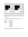
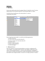
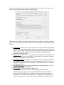
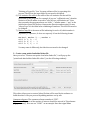
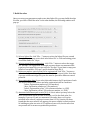
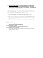
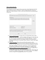
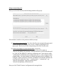
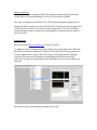
Image acquisition. Co-­‐stain with anti-­‐Even-­‐skipped 2B8 (1:50, often this needs to be pre-­‐absorbed several times for optimal staining], or 3C10 (1:50) available at DSHB. Use stage 16 embryos see Pereanu et al., 2007 for morphological staging criteria. Images should be acquired at least 8-­‐bit (512x512) resolution or better using a 60x or 63x objective and 0.3 to 0.5 microns steps. Segments T2, T3 and A1 should be included. Images can be cropped (e.g. using ImageJ) to eliminate regions without cells of interest. Segmentation. First start Vaa3d (http://Vaa3d.org/; Peng et al., 2010). To segment cells in an image stack, drag and drop the image stack into Vaa3d. The file will be opened and displayed. Then you choose from Vaa3D Plug-­‐In menu the “image_segmentation” plug-­‐in. Then you choose “Cell_Segmentation” and then “segment all image objects (adaptive thresholding followed by watershed)”. Note: these are not currently present in the Windows release; this is available for Mac only. After that, a window for parameter setting will pop up: Channel: You need to specify which channel you want to segment. Channel number starts from 1. Smoothing: You need to adjust “Median filter size”, “Gaussian filter size”, and “Gaussian filter sigma” to reduce noises in your image before segmentation. Thresholding: You may choose “Adaptive”, “Global (3D)”, and “Global (2D)” to separate background from signal. This information is used in later segmentation. Adaptive thresholding detects the threshold values at uniformly sampled pixels based on the statistical information of the local context, and then produces pixel resolution thresholds by interpolation. Global (3D) detects a unified intensity threshold value on all pixels, assuming the background level does is more or less constant across pixels in an image stack. Global (2D) is similar, but thresholds are computed for each 2D plane rather then a 3D volume and a smoothing step is applied to produce continuous thresholds between adjacent 2D planes. Segmentation Method: You may choose intensity-­‐based watershed or shape-­‐based watershed. The former is more sensitive to noise. Once you setup all the parameters, you may click “OK” button. The software will segment cells from the specified channel of the loaded stack. The result image will be displayed in another image window (see below). The segmented cells are displayed in gray. You may click “index” radio button on the right to display them in color. You may also use “See in 3D” function to visualize the cells in 3D. If the results are satisfactory (i.e., most nuclei are separated and there are few over-­‐
segmented nuclei/phantom objects) you may save it. Otherwise, you may change the parameters and retry. To save your result, choose “File” from Vaa3D menu, and then click “export”. At this point you should have four files for each channel; see below for example. All of the files associated with Eve should be placed in a single folder: In addition all of the files associated with additional markers should be placed in separate folders. The file names in each folder should be identical, for example: For each channel in the original image there is a: 1. .ano file It can be opened with a text editor. It contains the name of three associated files: GRAYIMG=10D07_1.tif.ano.gray.tif
MASKIMG=10D07_1.tif.ano.mask.raw
ANOFILE=10D07_1.tif.ano.apo
2. .tif file This is the original image data; it can be dragged into Vaa3d to be viewed. 3. .mask.raw file This is the result of segmentation; it can be dragged into Vaa3d to be viewed. 4. .apo file This can be opened with a text editor, or dragged into Vaa3d. It is a csv file with information about each segmented object: ##n,orderinfo,name,comment,z,x,y,pixmax,intensity,sdev,volsize,mass,,,, color_r,color_g,color_b
1, 1, A/10D07 T3R,, 45,191,179, 253.000,208.939,52.313,1983.000,414326.000,,,,251,38,17
2, 2, ,, 85,25,248, 253.000,195.720,61.394,3525.000,689914.000,,,,51,176,176
Annotation. Annotation is done using Vano software (update 1.9). A detailed users guide is available using the following link: http://vano.cellexplorer.org/how-­‐to-­‐use. This program opens the original .tif file, the segmented .mask.raw file and the .apo file with annotations for each object in a single interface. It allows the user to navigate through the images and insert annotations. Note that during annotation cell segmentation can be manually adjusted. Depending on the quality of the starting image the user may need to extensively manually edit the segmentation. It is important to have a single annotation for each cell of interest. Any updates will change the .mask.raw file as well as the .apo file. Also note if an object is left unannotated by the user, it will be ignored in subsequent steps. For the Even-­‐skipped pattern a user must annotate the following cells: aCC/eve T2L, aCC/eve T2R, aCC/eve T3L, aCC/eve T3R, aCC/eve A1L, aCC/eve A1R, pCC/eve T2L, pCC/eve T2R, pCC/eve T3L, pCC/eve T3R, pCC/eve A1L, pCC/eve A1R, RP2/eve T2L, RP2/eve T2R, RP2/eve T3L, RP2/eve T3R, RP2/eve A1L, RP2/eve A1R, U1/eve T2L, U1/eve T2R, U1/eve T3L, U1/eve T3R, U1/eve A1L, U1/eve A1R, U2/eve T2L, U2/eve T2R, U2/eve T3L, U2/eve T3R, U2/eve A1L, U2/eve A1R, U3/eve T2L, U3/eve T2R, U3/eve T3L, U3/eve T3R, U3/eve A1L, U3/eve A1R, U4/eve T2L, U4/eve T2R, U4/eve T3L, U4/eve T3R, U4/eve A1L, U4/eve A1R, U5/eve T2L, U5/eve T2R, U5/eve T3L, U5/eve T3R, U5/eve A1L, U5/eve A1R The easiest way to do this is to cut and paste from the cellnamelist_eve_nocluster.txt file found in the input folder (see below). The program does not tolerate typos, but does tolerate extra spaces at the beginning or end of the annotation. For other patterns a user must annotate any cell of interest with a unique cell name. The convention we use is as follows: “cellname/marker segment” e.g., aCC/eve T2L. Each cellname should also be listed in a text file named “cellnamelist_marker.txt”. Note creating a cellname list with hidden characters (when using Excel for example) can produce an error, so it is best to use a manual text editor to compile this file. The cellname file should be saved in the input folder [see below] with the name "cellnamelist_marker.txt". Vaa3D interface. The image is reproduced from Figure 1E,F. A list of the controls is given below. Panel E. Main window. (1) Object manager button; clicking this button opens the Object Manager window shown in panel F. (2) Surface cut; the default view for the 3D atlas data in the main window. (3) X, Y, Z rotation controls; spinning the analog dials rotates the 3D atlas around the indicated axis, and using the digital window below can be used for the same purpose. (4) Zero button; this realigns the 3D dataset to 0, 0, 0 degrees. Panel F. Object manager. This menu is used to select desired cells, manipulate cell color, add or read comments about the cells. It can be set to two formats: to manipulate individual cells by selecting the “Point Cloud” function (5), or to manipulate all the cells that express a single marker by selecting the “Point Cloud Set” function (6). Within each of these functions, the following controls can be used: (7) Select all; this selects all the cells or point clouds (markers), and once a cell/marker is selected you can apply a color to it, or manipulate it in other ways. (8) Select none; this de-­‐selects all selections. (9) Select inverse; this toggles selected to deselected, and deselected to selected. (10) On/off; “on” adds the selected cell/marker to the atlas view display in panel A; “off” takes the selected cell/marker out of the display. (11) Color; clicking this button opens the color choice window (red line to left) with three choices: “Single Color...” allows you to choose a single color to apply to the selected cells/markers, “Hanchuan’s Color Mapping” automatically assigns a pre-­‐ordered color selection uniquely mark each cell/marker selected, and “Random Color Mapping” gives every cell/marker a random color. (12) Name/Comments; this button brings up a window allowing the user to edit the name/comments fields. (13) Undo; this button reverses the last action. (14) “Accumulate...” allows sequential search strings using field (19) to accumulate. (15) On/off column; the boxes in this column show selected cells/markers. They can be toggled individually or using the controls (5-­‐7). (16) Color column; shows the color the cell/marker presents in the display. (17) Name; this column shows the cell/marker name. (18) Comment; this column shows the markers expressed by each cell. (19-­‐21) Search function. Type search query (19), and select either “next” to find the next occurrence of the search term, or previous to find the previous occurrence (20), or “Highlight all hits” (21) which highlights all occurrences of the term. After the search terms are highlighted they can be selected/deselected by using buttons (7-­‐8). Successive searches can be combined by toggling the “Accumulate...” button (14) prior to starting the search. Registration. 1. Main menu Put the atlas_builder plug-­‐in into the plugins folder for Vaa3d (Mac only). The atlas builder plug-­‐in can be found in Supp File 5. Users Manual folder as a .zip file. Click Plug-­‐in from Vaa3D menu, select atlas_builder. You will see “pointcloud_atlas_builder”. Select “pointcloud_atlas_builder”, you will see the following functions: 1) Adjust preference 2) Create a new point cloud atlas linker file 3) Edit an existing point cloud atlas linker file 4) Build the atlas 5) Detect coexpressing cells 6) Merge coexpressing cells 7) About this plugin 2. Adjust preference The basic parameters used for the atlas builder are saved in a configuration file ‘atlas_config.txt’. You can find this file under the ‘atlas_builder’ folder that you put under ‘v3d_external/bin/plugins/’ or ‘v3d_external/v3d/plugins/’ (depending on your version of Vaa3D). Currently this file contains the information used for running atlas builder on an example machine. You need to run “Adjust preference” function only once to setup your own. Once the parameters are set, you do not need to reset them unless you rename your files or move the data. When you select “Adjust preference” from the menu, you will see the above window pop up. The program reads the information in “atlas_config.txt” and fills them in the screen. 1) Input folder is where the user puts input files, such as cellname lists that tells the computer what cell names to expect. The user needs to create a file called “input”. In the “input” folder place all of the files from “input.zip” found in the Users Manual section of the supplemental methods. Using the “Folder…” navigate to the input folder. 2) Output folder is where the user puts files produced by the atlas builder, such as linkers and new .apos (see below). Create a file called “output”. Using the “Folder…” navigate to the output folder. 3) Cell name file prefix is the prefix of cell name lists. For example, the names of cells expressing AP markers are saved in “cellnamelist_ap.txt”. So cell name file prefix is ‘cellnamelist’. This is shared by all the markers. There is no need to change this field. 4) Cell name file suffix is the suffix of cell name lists. In this example, it is ‘.txt’. There is not need to change this field. 5) Cell type file is a list of cell type file names, e.g., “cellname_type_interneuron.txt”, “cellname_type_motoneuron.txt”, “cellname_type_secretory.txt”. You can find them in your input folder. To remove any of these files click the “Remove” button on the right. Then you click the “File …” button on the right of the “cell type file:”. It will pop up a window allowing you to select a file. The selected file will be added into the “Existing cell type file:” box. You may add more files by repeating this process. The files in the input folder do not need to be edited. 6) Cell statistics file suffix is the suffix of the cell statistics file that will be generated by the program. For example, if you use “cellStatistics.txt”, then the statistics of the AP maker is saved in “atlas_AP.apo_cellStatistics.txt”. Note that currently the program always use “atlas_” + marker name + “.apo” as the initial atlas output file (before coexpression detection and merging). It uses “atlas_all.apo” as the initial atlas combining all markers. This does not need to be changed. 7) Marker map file is the name of file indicating for each cell, which marker it expresses (1: expresses, 0: does not express). It has the following format: Marker1, marker 2, …, marker n
Cell 1: 1, 0, … 0
Cell 2: 0, 1, … 1
Cell 3: 1, 1, …. 0
You may name it differently, but this does not need to be changed. 3. Create a new point cloud atlas linker file Once you select “Create a new point cloud atlas linker file”, it will pop up the “pointcloud atlas builder linker file editor” (see the following window): This editor allows you to create a linker file that will be used by the software to build the atlas. It lets you proceed by adding markers one by one. Common reference. The common reference marker is “EVE”. Signal name. The name of the marker of interest should be entered in “Signal name (e.g. gene name)”. Here we use “10D07” as an example. Note that signal name “10D07” corresponds to “cellnamelist_10D07.txt”, created as described in the "Annotation" section. Signal folder is where the marker channels of your annotated marker image stacks are saved (.apo; generated by manual annotation using VANO software, using the names deposited in the cellnamelist_eve_nocluster.txt). Reference folder is where the reference channels (EVE) of the dataset are saved. As mentioned above, file names in the signal (ch2_10D07) and reference (ch1_eve) should be identical. To select these folders, you need to click the “Folder…’ buttons to the right of “Signal folder” and “Reference folder”. The software will automatically test if the files in signal folder match those in the reference folder. If any mismatch occurs, for example, a particular stack has only a marker channel but no reference channel, the font in the two text area on the right of “Folder” will be changed to red. You need to check the problem of your data before moving on to the next step. If no error is found, the marker added will be displayed in the text area below. You can click “Add a new signal” to add another marker, or click “Finish” to end adding new markers. Once you click finish, a window allowing you to select where the linker file should be saved will pop up. You may put it under your output folder. 4. Edit an existing point cloud atlas linker file After you create the atlas linker file, you may need to add new markers as your data accumulate. This can be achieved by clicking “Edit an existing point cloud atlas linker file” and choosing the linker file that you want to edit. It pops up a window similar to the one when you create a linked file, but can display all the existing markers in the linker file. You may follow the same steps you used in creating the linker file. 5. Build the atlas Once you setup your parameters and create atlas linker file, you may build the atlas. For that, you select “Build the atlas” in the atlas builder, the following window will pop up: 1) Select a linker file: click “File …” button to select the linker file you created through “Create a new point cloud atlas linker file” or “Edit an existing point cloud atlas linker file” steps. 2) Select a target file for registration: click “File…” button to select the target file “Eve.apo” for registration. Although you may choose any annotated file (.apo) as your target file, you can only use “Eve.apo” if you want to map your atlases to our atlases. “Eve.apo” can be found in Supp File 2. 3) Reference marker control point file for registration: click “File…” button to select the “cellnamelist_eve_nocluster.txt” under your input folder. Note that if you use a different target file, you also need to provide a different control point file. 4) Save registration data: if you select this radio button, the 3D positions of each cell in each image stack before and after registration will be saved into: “before_registration_marker.txt” (for markers) “after_registration_marker.txt” (for markers) “before_registration_ref.txt” (for reference marker, i.e., EVE) “after_registration_ref.txt” (for reference marker, i.e., EVE) 5) Annotated stack must pass a ratio (0-­‐1) of: this is where you may select the ratio of annotated stacks in order to include a cell in the final atlas. For example, if you set 0.3 and you annotated 10 stacks, then a cell can be included in the atlas if it appears in more than 0.3*10=3 stacks. We have found that the more often a cell appears, the more reliable its final position. So building an atlas at a ratio of 0.5 will have fewer cells, but the ones that are present will be at more reproducible positions. 6) Select force added cell file: select the file that list the cells that must be included into the atlas no matter the annotated ratio. You don’t have to provide this file if you don’t force any cell to be included. You can find a list of forceAddCells in the input folder. After setting up these parameters, you click OK. The program will run and generate the initial atlas shortly. You may find your results under the output folder that you’ve setup in the “Adjust preference” step. 1) For each marker, the atlas is named by “atlas” + marker + “.apo”. 2) The initial atlas that combines all the markers is named by “atlas_all.apo” 3) The statistics of cells expressing each marker is saved in “atlas” + maker + “.apo_cellStatistics.txt” 4) The atlases of different cell types are named by “atlas”+celltype+”.apo” Common errors 1)"Build the atlas" hangs Did you create cellnamelist_marker.txt? 2)"atlas_marker.apo" is empty cellnamelist_marker.txt may have hidden characters. 3)Standard deviation is really large Possible mis-­‐annotation of a cell identity, or the segment is off-­‐by-­‐one relative to the Eve channel. Detect coexpressing cells. The initial atlas you build using the above steps may contain duplicated cells that express different markers. You may use “Detect coexpressing cells” function to detect the co-­‐expressing cells. Once you select this function, the following window will pop up: 1) Select an atlas file (.apo): You may select a set of atlas files to detect their coexpression. Click “File…”, it opens a window allowing you to select an atlas file. The selected file will be shown in the “Existing atlases are: “ box. You may select multiple atlas files. You may also remove any of them by first selecting the files in the box and then click the “Remove” button on the right hand side. 2) Coexpression rules: Three rules are used by the program to detect coexpression. You may define the distance between coexpressing cells. You may also selecting symmetry (if two cells in the left hemisegment coexpress, their right hemisegment parterners should also coexpress) and bilateral (coexpressing cells must be in the same hemisegment, or midline) rules. 3) Prefix of the names of output coexpression files: if you use “AP_EN_EVE” in the above window, the two output coexpression files are: “AP_EN_EVE.coexpress.apo” and “AP_EN_EVE.coexpress.txt”. The former can be viewed by dragging and dropping to the Vaa3D 3d viewer. The candidate cells that coexpress are highlighted by white. The second file “AP_EN_EVE.coexpress.txt” save the detail information of the coexpressed cells. One you set up these parameters, click ‘Finish’ button, the program will produce the predicted coexpressing cells in a second. Your job is to check the AP_EN_EVE.coexpress.apo and AP_EN_EVE.coexpress.txt and generate a manually curated file (text format) listing the confirmed coexpressing cells. The format of this new text file is: final cell name: cell name in marker A, cell name in marker B, … For example: aCC A1L: aCC/pMAD A1L, aCC/eve A1L, aCC A1R: aCC/pMAD A1R, aCC/eve A1R, BDL1 A1L: BDL1/pMAD A1L, BDL1/bar A1L, BDL1 A1R: BDL1/pMAD A1R, BDL1/bar A1R, Also see, cellname_mapping.txt in the input folder. This file will be used in “Merge coexpressing cells” (see below). Merge coexpressing cells. Once you select this function, the following window will pop up: This window is similar to the previous window, except: 1) Select the coexpression file: You select the file semi-­‐automatically generated by the last step. For example, here we use “cellname_mapping.txt” we generated. This file lists all the coexpressing cells in the current atlas. 2) Prefix of the names of output merged files: If you use “atlas_AP_EN_REPO_PS1_final”, then the final atlas will be name as “atlas_AP_EN_REPO_PS1_final.apo”, and the statistics of cells in this atlas will be: “atlas_AP_EN_REPO_PS1_final.apo_cellStatistics.txt”. Note that the suffix “cellStatistics” is defined in your configuration file, i.e., atlas_config.txt under plugins folder. You may change it by simply editing the atlas_config.txt or by using the “Adjust preference” function. In addition, each marker will have its own final atlas, named by “atlas_” + marker name + “_merged.apo”, e.g., “atlas_AP_merged.apo”, and the statistics file is “atlas_AP_merged.apo_cellStatistics.txt”. Once you click “Finish” button, it will generate the merged atlas.