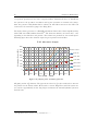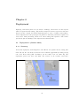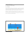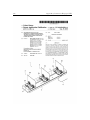
1
Power Take-off System
Design for Wing-Wave
WEC
by
Ismail Sultan
Bachelor of Engineering
Industrial Electronics
NED University of Engineering and Technology
Karachi, Pakistan
2004
A thesis submitted to
the Department of Marine and Environmental Systems
at Florida Institute of Technology
in partial fulfillment of the requirements for the degree of
Master of Science
In
Ocean Engineering
Melbourne, Florida
July, 2013
© Copyright 2013 Ismail Sultan
All Rights Reserved
The author grants permission to make single copies
i
ii
We the undersigned committee hereby recommends that
the attached document be accepted as fulfilling in part the requirements for the degree of
Master of Science in Ocean Engineering
Power Take-off System Design for Wing-Wave WEC
by
Ismail Sultan
Stephen Wood, Ph.D., P.E.
Associate Professor
Ocean Engineering Program Chair
Marine and Environmental Systems
Major Advisor, Committee Chair
George A. Maul, Ph.D.
Professor and Department Chair
Marine and Environmental Systems
Committee Member
Hector Gutiérrez, Ph.D., P.E.
Associate Professor
Mechanical and Aerospace Engineering
Committee Member
iii
iv
Abstract
Power Take-off System Design for Wing-Wave WEC
by
Ismail Sultan
Major Advisor: Stephen Wood, Ph.D., P.E.
The oceans represent a massive untapped energy resource with
potentially more energy than the aggregated output of all other resources
on the earth. In recent years, there has been a growing focus globally on
the development of economical and efficient conversion technologies for
the ocean energy.
The work in this thesis presents a system for power conversion and
extraction, truning the ocean’s waves energy into electrical energy. The
main goal of the study was to design, and develop a P ower Take-off
system for the ‘Wing-Wave’, a flap-type sea-bed mounted wave energy
converter (WEC). The power take-off system consisted of hydraulic,
electrical and control subsystems to evaluate the performance of WingWave. The wave energy was captured in form of hydro-mechanical
energy by the pistons coupled with the flap of Wing-Wave. This
hydraulic energy was then converted to electrical energy by an impulsetype turbine. The control system was designed with wireless data
acquisition capability for the remote viewing and control.
Full scale prototypes of the power take-off system were deployed and
tested using the Wing-Wave in the summer of 2012 and 2013. The
prototypes successfully demonstrate the wave energy capture in the
deployment.
Index Terms— Ocean Energy, Wave Energy, Wave Energy Convertors,
Wireless, P ower take-off, Renewable energy
v
vi
"I am a citizen of the most beautiful nation on earth,
a nation whose laws are harsh yet simple,
a nation that never cheats,
which is immense and without borders,
where life is lived in the present.
In this limitless nation, this nation of wind, light, and peace,
there is no other ruler besides the sea."
--Bernard Moitessier
vii
viii
Table of Contents
Abstract ...................................................................................................................................... v
Table of Contents ...................................................................................................................... ix
List of Figures.......................................................................................................................... xiii
List of Tables ............................................................................................................................ xv
List of Symbols ........................................................................................................................ xvi
Constants ........................................................................................................................... xviii
Variables ............................................................................................................................ xviii
List of Equations ..................................................................................................................... xvi
Acronyms ................................................................................................................................. xix
Dedication ................................................................................................................................ xxi
Preface ................................................................................................................................... xxiii
Part I Problem Introduction and Background .......................................................................... 1
Chapter 1
Introduction ........................................................................................................... 3
1.1
Motivation.................................................................................................................. 3
1.2
Problem Statement .................................................................................................... 5
1.3
Scope and objectives .................................................................................................. 6
1.4
Outline of the Thesis ................................................................................................. 7
Chapter 2
2.1
Theory .................................................................................................................... 9
Fluid Mechanics ......................................................................................................... 9
2.1.1
Bernoulli’s Equation .............................................................................................. 9
2.1.2
Buoyancy ............................................................................................................... 9
2.1.3
Viscosity ............................................................................................................... 10
2.1.4
Reynolds Number ................................................................................................ 10
2.1.5
Drag ..................................................................................................................... 10
2.2
Wave Basics ............................................................................................................. 11
2.2.1
Wave characteristics ............................................................................................ 11
2.2.2
Creation of waves ................................................................................................ 12
2.2.3
Linear theory of ocean waves .............................................................................. 13
2.2.4
Wave Shoaling ..................................................................................................... 14
2.2.5
Wave energy ........................................................................................................ 14
ix
2.3
Chapter 3
Power Take-off ......................................................................................................... 15
Project Background ............................................................................................. 17
3.1
History ...................................................................................................................... 17
3.2
Classification ............................................................................................................ 19
3.3
Current Commercial-scale WEC ............................................................................. 21
3.4
Interest in Near-to-shore and Flap-type Convertors............................................... 22
3.5
Wave energy research at FIT .................................................................................. 23
3.5.1
Wing-Wave .......................................................................................................... 23
Part II Hardware Design and Construction............................................................................. 27
Chapter 4
Methodology......................................................................................................... 29
4.1
Design Requirements ............................................................................................... 29
4.2
Power Take off System – Control Design ............................................................... 32
4.2.1
Control and Data Acquisition Module ................................................................ 32
4.2.2
Instrumentation ................................................................................................... 38
4.2.3
Communication .................................................................................................... 41
4.2.4
Control Algorithm ............................................................................................... 41
4.3
4.3.1
Power Take off System – Electrical Design ............................................................ 43
Control Supply and solar panel ........................................................................... 43
4.4
Power Take off System – Hydraulic Design............................................................ 45
4.5
PTO Raft Design ..................................................................................................... 47
Part III Testing and Deployment ............................................................................................ 49
Chapter 5
Laboratory Testing .............................................................................................. 51
5.1
Generator Testing .................................................................................................... 51
5.2
Wing-Wave and Piston Testing .............................................................................. 52
5.3
PTO Testing ............................................................................................................ 53
Chapter 6
6.1
Deployment .......................................................................................................... 55
Deployment 1 (Summer 2012) ................................................................................. 55
6.1.1
Summary .............................................................................................................. 55
6.1.2
Results .................................................................................................................. 56
6.1.3
Weather and Wave data ..................................................................................... 58
6.1.4
Data recorded....................................................................................................... 59
6.2
6.2.1
Deployment 2 (Summer 2013) ................................................................................. 61
Summary .............................................................................................................. 61
x
6.2.2
Results.................................................................................................................. 62
6.2.3
Weather and Wave data ..................................................................................... 64
6.2.4
Data Recorded (PTO) ......................................................................................... 65
6.2.5
Data recorded (Accelerometer) ........................................................................... 68
Part IV Mathematical Modeling .............................................................................................. 69
Chapter 7
Mathematical formulation and Validation ......................................................... 71
7.1
Governing equations for the Flap type WEC ......................................................... 71
7.2
Wave Force Calculations on Wing-Wave ............................................................... 74
7.2.1
Equation of Motion ............................................................................................. 74
7.2.2
Wing-Wave Design and Assumptions ................................................................. 75
7.2.3
Wave Orbital calculation .................................................................................... 77
7.2.4
Wave Force calculation (McCormick) ................................................................ 78
7.2.5
Capture Width Calculation ................................................................................. 80
7.2.6
Surge Wave Force Calculation ............................................................................ 80
7.3
Morrison Equation and Force Coefficients ............................................................. 81
7.4
Force Calculations on Piston .................................................................................. 83
7.5
Hydraulic Work done by the Piston ....................................................................... 86
7.6
Hydraulics - Accumulators ...................................................................................... 87
7.7
Deployment Result Validation ................................................................................ 89
Part V Conclusion.................................................................................................................... 91
Chapter 8
Future Research................................................................................................... 93
8.1
Simulation and Modeling ........................................................................................ 93
8.2
Hydraulics and Instrumentation ............................................................................. 93
8.3
Wave Tank Testing ................................................................................................. 94
8.4
Power System .......................................................................................................... 94
Chapter 9
Conclusion............................................................................................................ 95
References ................................................................................................................................. 97
Appendix 1: Publications ........................................................................................................103
Appendix 2: Code ................................................................................................................... 107
A2.1
Raspberry Pi / Python...................................................................................... 107
A2.2
Arduino .............................................................................................................. 110
A2.3
Visual Basic ........................................................................................................... 117
xi
Appendix 3: Patents for Flap-type WEC .............................................................................. 123
xii
List of Figures
Figure 1-1: Annual average estimated global wave power in kW/m (Barstow and Kabuth
2010) ........................................................................................................................................... 4
Figure 1-2: (Left) Wing-Wave WEC (Right) GECCO WEC................................................... 5
Figure 1-3: Thesis Scope (Wing-Wave WEC and PTO System) ............................................. 6
Figure 1-4: Basic Energy Flow Diagram for Wing-Wave WEC (Khan et al. 2008) ................ 7
Figure 2-1: Wave Characteristics (Bostrom 2011) ............................................................... 11
Figure 2-2: Wave formation in ocean ...................................................................................... 12
Figure 2-3: Wave Orbitals........................................................................................................ 14
Figure 2-4: PTO types ............................................................................................................. 15
Figure 3-1: Patent by Girad in 1799 (Polinder and Scuotto 2005) ........................................ 17
Figure 3-2: Different types of Wave Energy Technologies (Falcão 2010) .............................. 20
Figure 3-3: Illustrations for types of wave energy technologies (Pecher 2012)....................... 20
Figure 3-4: Photographs of commercial WEC (in order of Table 3-1) ................................... 21
Figure 3-5: Average gross and exploitable wave power at three water depths (Cameron et al.
2010) ......................................................................................................................................... 22
Figure 3-6: (Top Left, Clockwise) Wing-Wave Prototypes for year 2008 (model), 2010, 2011
and 2012/13 .............................................................................................................................. 24
Figure 4-1: Functional block diagram of the project............................................................... 30
Figure 4-2: (Left) Control and data acquisition System (Middle) Moxa® W5340i Controller
(Right) ActiveOPC Server software ........................................................................................ 32
Figure 4-3: Control Diagram for the first deployment ............................................................ 33
Figure 4-4: Control Diagram for the second deployment........................................................ 34
Figure 4-5: (Right) Control panel for the second deployment (Left) Close-up shot of cards 35
Figure 4-6: Visual Basic based HMI ........................................................................................ 37
Figure 4-7: (Left) Pressure Sensor (Middle) Exploded view of Flowmeter (Right)
Proportional Control Valve...................................................................................................... 39
Figure 4-8: Accelerometer ........................................................................................................ 40
Figure 4-9: Hydraulic Diagram (2012 Deployment) ................................................................ 45
Figure 4-10: Output power for Harris generator ..................................................................... 46
Figure 4-11: Hydraulic system in PTO raft (2013) ................................................................. 47
Figure 4-12: Layout for the PTO Raft .................................................................................... 47
Figure 4-13: PTO Raft Design (Deployment 2012) ................................................................ 48
Figure 4-14: PTO Raft Design (Deployment 2013) ................................................................ 48
Figure 5-1: Results for the mechanical testing of Harris Hydroelectric Generator ................ 51
Figure 5-2: Results for the process testing of Harris Hydroelectric Generator....................... 52
Figure 5-3: Land testing of Wing-Wave .................................................................................. 53
Figure 5-4: PTO system being tested with utility water ........................................................ 53
Figure 5-5: Dataset for PTO testing (1) .................................................................................. 54
Figure 5-6: Dataset PTO testing (2) ....................................................................................... 54
Figure 6-1: Deployment Location ............................................................................................ 55
xiii
Figure 6-2: Deployment configuration for 2012 ....................................................................... 56
Figure 6-3: PTO raft during deployment................................................................................. 57
Figure 6-4: Wing-Wave during deployment ............................................................................ 57
Figure 6-5: Wave and Period rose for the deployment summer 2012 ..................................... 58
Figure 6-6: Datasets recorded in Deployment 2012 ................................................................. 60
Figure 6-7: Deployment Configuration for 2013 ...................................................................... 61
Figure 6-8: PTO raft during deployment ................................................................................ 63
Figure 6-9: Wing-Wave during deployment ............................................................................ 63
Figure 6-10: (Upper half) Wave and Period Rose for June 2013 (Lower half) Time series plot
for Wave Height and period ..................................................................................................... 64
Figure 6-11: Dataset recorded for deployment 2013 ................................................................ 66
Figure 6-12: Dataset recorded for deployment 2013 ................................................................ 67
Figure 6-13: Dataset recorded in the deployment 2013 ........................................................... 68
Figure 7-1: Geometry of the Flap type converter (a) section, (b) plan (Renzi and Dias
2012a) ........................................................................................................................................ 72
Figure 7-2: Wing-Wave and wave variables ............................................................................ 76
xiv
List of Tables
Table
Table
Table
Table
Table
Table
Table
2-1:
4-1:
4-2:
4-3:
4-4:
4-5:
7-1:
Ocean Wave Types ................................................................................................. 11
Specifications for Raspberry Pi Model B ............................................................... 35
Specifications for Arduino AT Mega2560 ............................................................. 36
Input Map ............................................................................................................... 38
Output Map ............................................................................................................ 38
Current Consumption ............................................................................................. 44
Datasets for deployment 1...................................................................................... 59
xv
List of Equations
2-1................................................................................................................................................ 9
2-2................................................................................................................................................ 9
2-3.............................................................................................................................................. 10
2-4.............................................................................................................................................. 10
2-5.............................................................................................................................................. 13
2-6.............................................................................................................................................. 13
2-7.............................................................................................................................................. 14
2-8.............................................................................................................................................. 14
7-1 ............................................................................................................................................. 72
7-2.............................................................................................................................................. 72
7-3.............................................................................................................................................. 72
7-4 ............................................................................................................................................. 73
7-5 ............................................................................................................................................. 73
7-6 ............................................................................................................................................. 73
7-7 ............................................................................................................................................. 74
7-8 ............................................................................................................................................. 74
7-9 ............................................................................................................................................. 77
7-10............................................................................................................................................ 77
7-11............................................................................................................................................ 77
7-12............................................................................................................................................ 77
7-13............................................................................................................................................ 77
7-14............................................................................................................................................ 78
7-15............................................................................................................................................ 78
7-16............................................................................................................................................ 78
7-17............................................................................................................................................ 78
7-18............................................................................................................................................ 78
7-19............................................................................................................................................ 79
7-20............................................................................................................................................ 79
7-21............................................................................................................................................ 79
7-22............................................................................................................................................ 79
7-23............................................................................................................................................ 79
7-24............................................................................................................................................ 79
7-25............................................................................................................................................ 79
7-26............................................................................................................................................ 80
7-27............................................................................................................................................ 80
7-28............................................................................................................................................ 80
7-29............................................................................................................................................ 80
7-33............................................................................................................................................ 81
7-30............................................................................................................................................ 81
7-31............................................................................................................................................ 81
xvi
7-32 ........................................................................................................................................... 81
7-34 ........................................................................................................................................... 82
7-35 ........................................................................................................................................... 82
7-36 ........................................................................................................................................... 83
7-37 ........................................................................................................................................... 84
7-38 ........................................................................................................................................... 84
7-39 ........................................................................................................................................... 84
7-40 ........................................................................................................................................... 84
7-41 ........................................................................................................................................... 84
7-42 ........................................................................................................................................... 84
7-43 ........................................................................................................................................... 84
7-44 ........................................................................................................................................... 85
7-45 ........................................................................................................................................... 85
7-46 ........................................................................................................................................... 86
7-47 ........................................................................................................................................... 86
7-48 ........................................................................................................................................... 86
7-49 ........................................................................................................................................... 86
7-50 ........................................................................................................................................... 87
7-51 ........................................................................................................................................... 87
7-52 ........................................................................................................................................... 87
7-53 ........................................................................................................................................... 88
7-54 ........................................................................................................................................... 88
7-55 ........................................................................................................................................... 88
7-56 ........................................................................................................................................... 88
xvii
List of Symbols
Constants
𝜋
3.141 592 654
e
2.718 281 828
g
9.81 m=s2
Variables
𝑎
Amplitude of wave ................................................................................. [m]
CM
Inertia coefficient ...................................................................................... [-]
𝐵𝑓
𝐶𝐷
𝑓
𝑔
ℎ
ℎ1
ℎ𝑓
ℎ𝑝
𝐻
𝑘
𝐿
𝐿𝑓
𝑀𝑓
𝑉𝑓
𝑡𝑓
𝑇
𝜌𝑓
𝜌
𝜔𝜔
𝜈
Width of Flap .......................................................................................... [m]
Drag coefficient ........................................................................................ [-]
frequency................................................................................................. [Hz]
2
gravity................................................................................................. [m/s ]
Depth ....................................................................................................... [m]
Distance between top of flap and surface ............................................... [m]
Height of Flap.......................................................................................... [m]
Height of Piston Connection ................................................................... [m]
Wave Height ............................................................................................ [m]
-1
Wave Number ....................................................................................... [m ]
Wavelength .............................................................................................. [m]
Stroke length ........................................................................................... [m]
Mass of Flap ........................................................................................... [kg]
3
Flap Volume ........................................................................................... [m ]
Flap Thickness......................................................................................... [m]
TimePeriod ................................................................................................ [s]
3
Flap density ...................................................................................... [kg/m ]
3
Density .............................................................................................. [kg/m ]
Angular Frequency ................................................................................ [rad]
Kinematic Viscosity............................................................................ [m²/s]
xviii
Acronyms
ADC
ARM
FIT
WEC
RTC
LPM
I/O
Analog digital converter
ARM (formerly Advanced RISC Machine)
Florida Institute of Technology
Wave Energy Convertor
Real Time Clock
Liter per Minute (Flow)
Input and Output
xix
xx
Dedication
To my Ammi and Abbu
All that I have achieved yet in my life and
will ever achieve in coming days,
I owe to them.
xxi
xxii
Preface
“You can put a teddy bear out in waves, and it will absorb energy."
-Brian Count (Scher, 1985)
This thesis is part of my effort to understand the energy behind the bobbing teddy bear in
the waves. The time period was short but the experience and the learning are going to stay
with me for much longer time.
I humbly consider myself very fortunate to have support of so many people in my personal
and academic life for the completion of my Masters. First of all, I would like to express my
gratitude to Fulbright Program and U.S. Department of State for giving me an opportunity
to come to US and complete my Masters.
Then I am extremely thankful to my advisor, Dr. Stephen Wood, for all his support,
patience and and supervision during my study. I am also grateful to my thesis committee
members, Dr. George Maul and Dr. Hector Gutierrez for their guidance and valueable
suggestions.
I would like to thank Dr. Robert Weaver and Dr. Prasanta K. Sahoo for their great support
during this project.
I would also like to acknowledge the generous help by Mr. Lee Marcum (SebaiCMET, Inc,
Clean and Green Enterprises, Inc) and Mr. S Ibne Hasan (Intech Automation). I am also
thankful to Mr. Bill Battin for his help on very short notices.
I had honor of working with two undergraduate student teams during this thesis and I am
very grateful for their tremendous effort throughout the construction and deployment of the
Wing-Wave. For 2012: Billy, Patrick, Sitara, Mario, Chad and Alexej; For 2013: Tolu,
Abbie, Jacob, Hallana, Kevin and Marine.
Also I am greatly indebted to my grad lab fellows, Matthew Jordan and Anthony, Jones for
their time, assistance and help.
In end, a very special thanks goes to the person without whose support and sacrifices it
would not have been possible for me to get this done: my better half, Madiha. She was not
present physcially with me during this time but it was her support that kept me going
through some real tense parts of my study.
Ismail Sultan
July 28, 2013
xxiii
Part I
Problem Introduction and Background
1
Chapter 1
Introduction
Throughout the history, the oceans have greatly influenced the way mankind has survived
and evolved. The climate and the weather system, on which the human race depends for its
survival, is a result of the interaction between the ocean and the atmosphere. The ocean
cover more than three quarters of Earth (Nybakken and Webster 1998). As of today, over
half of the world population lives less than 200 kilometers away from the oceans (Hinrichsen
1999).
The enormous size of the oceanic bodies and processes may have the hidden answer to the
energy appetite of the world. Maybe the ‘blue’ solution is the sustainable, environment
friendly and reliable solution our future generations would need.
This is the domain in which this work attempts to contribute. The following parts of this
chapter will present the motives for the present study, as well as, a statement of the
problem to be addressed
1.1
Motivation
Depletion of fossil fuel reserves and environmental disasters have changed the global attitude
toward energy issues. A major future energy crisis is seen only as a matter of time if the
dependency on fossil fuels as main source of energy doesn’t change soon. The exponential
growth in human population and resulting high energy demands may deplete the currently
known fossil fuel reserves in 40 years (Shafiee and Topal 2009). The awareness of this danger
has resulted in a significant shift of energy research towards renewable energy resources.
3
4
Chapter 1: Introduction
One of the major renewable energy resources, in addition to wind and solar, is ocean energy.
The oceans cover almost 360 million square kilometers i.e. approximately 72% of the Earth
(Nybakken and Webster 1998). They represent an enormous untapped energy resource
containing potentially more energy than the aggregated output of all other resources on the
earth. It is estimated that the theoretical potential of the ocean related energies is up to 2
Million Terawatt-hours (UNDP 2000).
Ocean energy is actually a derived form of solar energy and result of complex wind-wave
interactions (Knauss 2005). Ocean Energy is stored partly in the form of kinetic energy
from the motion of waves and currents and partly as thermal energy from the sun. Different
forms of Ocean energy are thermal, salinity, currents, tidal and wave. Out of these forms,
wave and tidal have been in the limelight of R&D efforts because of the abundance and
broad access (Bard and Schmid 2005). Compared to other renewables resources, wave
energy has a higher energy density, a higher availability and better predictability (Brekken
and Han 2009). Figure 1-1 shows world map with the potential wave power as kW/m of the
wave front.
Despite the enormous potential of ocean energy, there are some major obstacles due to
which the development of ocean energy technology lags when compared to those for solar
and wind. The challenges include the inherent unstable and uncertain nature of ocean
energies, accessibility and extreme weathers. These result in stringent engineering design
requirements and eventually relatively higher costs for ocean energy research. Increasing
Figure 1-1: Annual average estimated global wave power in kW/m (Barstow and
Kabuth 2010)
1.2 Problem Statement
5
power quality demands for the power grid integration adds to the complexity of the
problem. These issues also lengthen the design cycle time required for new technology
development.
For the researchers working in the field of ocean energy, reliable, low-cost and effective
evaluation of the ocean energy conversion technologies is critical for their successful and
smooth integration into the large power systems. These tools are indispensable for concept
verifications on a small-scale (e.g., research and development) and can assist in the rapid
and successful transformation of ocean renewable energy technologies from prototype to fullscale matured systems.
1.2
Problem Statement
The Ocean Engineering Department at Florida Institute of Technology (FIT) is currently
working on two prototypes of Wave Energy Convertors (WEC): Wing-Wave, a sea-bed
mounted bottom hinged type WEC that captures energy from the horizontal component of
wave orbitals at varying depths and GECCO, a surface floating attenuation WEC for
harnessing surface waves.
Concept verification of these WEC’s designs was done in 2010 and 2011. Sea-test scale
models were developed and successfully deployed. However, no Power Take-Off (PTO)
system was designed to capture the energy and convert it to electricity. Furthermore there
was limited instrumentation on these WECs, which was not sufficient to understand the
operational performance completely.
In 2012 and 2013, focus of the work on the Wing-Wave and GECCO was broadened to
develop a basic Power Take-Off (PTO) for the evaluation of the electrical generating
potential of the devices. Later in 2013, it was decided to focus on Wing-Wave only for
Figure 1-2: (Left) Wing-Wave WEC (Right) GECCO WEC
6
Chapter 1: Introduction
development to save efforts and time.
1.3
Scope and objectives
The main goal of this thesis is to evaluate the wave energy capture potential of the WingWave through testing and real-sea deployment. To achieve this goal, following objectives
were set:
1.
2.
3.
Design and development of a complete ‘Power Take-off’ system for deployment
with Wing-Wave. This would include:
a. Hydraulics system
b. Instrumentation and control valves
c. Power system for the electrical load
d. Control and data acquisition system (with wireless connectivity )
e. Human Machine Interface Software for real-time viewing.
Ocean deployment of the PTO with Wing-Wave and real-time data acquisition.
Development of a mathematical framework for the Wing-Wave WEC, and
Power Take-Off System (including the hydraulic systems).
Figure 1-3 shows the scope of this thesis. Work flow of the combined Wing-Wave and PTO
system is as following: Wave energy is converted into hydro-mechanical energy by the
pistons connected with the flap of Wing-Wave, which drives a Pelton/impulse turbine
coupled with an alternator. The energy is then fed into the power module that regulates the
electrical output. The control system controls the hardware, records instrumentation data,
and sends data via the wireless connection. The user is able to monitor the real-time data
through the Human Machine Interface (HMI) software and send commands remotely. The
power take-off system is housed in a floating raft anchored at the surface near the wave
energy converters during testing. Figure 1-4 shows the overall energy flow of the system
Figure 1-3: Thesis Scope (Wing-Wave WEC and PTO System)
1.4 Outline of the Thesis
7
Figure 1-4: Basic Energy Flow Diagram for Wing-Wave WEC (Khan et al. 2008)
from wave-to-wire.
Note: The work in this thesis doesn’t include any grid connectivity related issue due to
limited time and resources.
1.4
Outline of the Thesis
This thesis is divided into 9 chapters. Chapter 1 gives an introduction of the problem and
the goals set for this thesis.
In Chapter 2, an overview of important concept regarding the subject is presented which
includes the ocean waves, control/embedded systems, hydraulics and power. Chapter 3
presents the project background. It covers the literature reviewed, and an overview of the
work that has been done at Florida Institute of Technology on ocean energy.
Chapter 4 presents the hardware design for the system. Chapter 5 and 6 present the
laboratory testing and deployment of the system. Discussion on the results and observations
regarding deployment is included.
Chapter 7 presents the mathematical equations and framework needed to model a flap type
WEC. The forces acting on the flap and PTO are calculated using different approaches.
The last section of this document is on the further work required for the Wing-Wave and
the conclusion of the work done in this document.
8
Chapter 1: Introduction
Chapter 2
Theory
Before moving to the sections related to design and mathematical modeling of the system,
some basic concepts and terminologies will be introduced in this section. The first section
focuses on the concepts that are fundamental in understanding the mechanics behind the
Wave Energy Convertor. This includes the fluid mechanics, waves and marine
hydrodynamics.
The second part describes the technicalities of the Power Take-off system. An overview of
the electrical, control and hydraulic systems is presented.
2.1
Fluid Mechanics
2.1.1 Bernoulli’s Equation
Bernoulli's principle is actually a derived form of conservation of energy for fluid dynamics.
It relates the potential and kinetic energy for an inviscid steady flow. It is given as (Munson,
Young, and Okiishi 2002):
𝑝1 𝑣12
𝑝3 𝑣32
+
+ z1 = +
+ z3 + ℎ𝑠 − ℎ𝐿
𝜌 2𝑔
𝜌 2𝑔
2-1
Where ℎ𝑠 and ℎ𝐿 represent the head shaft and head loss respectively. The Bernoulli's
equation will be used for hydraulic system calculations.
2.1.2 Buoyancy
Buoyancy force is the upward force exerted by the fluid on a body immersed in it (Munson,
Young, and Okiishi 2002).
𝐵 = 𝜌𝑔𝑉𝑏𝑜𝑑𝑦
2-2
If the buoyancy force and the weight of the immersed body are equal then the body would
float in equilibrium. The body will sink if buoyancy is less and will rise if buoyancy is
greater as compared to its weight.
9
10
Chapter 2: Theory
2.1.3 Viscosity
Viscosity represents the resistance to flow offered by the fluid. Viscosity is due to inherent
friction resulting from the shear stress between adjacent layers of the fluid that are moving
at different velocities. A fluid with no resistance to shear stress is known as an inviscid fluid.
Dynamic viscosity is determined by the shear stress effect on the two adjacent layers of the
fluid. Kinematic viscosity is the ratio between dynamic viscosity and fluid density.
2.1.4 Reynolds Number
Reynolds Number 𝑅𝑒 is the measure of the ratio of inertial forces to the viscous forces in the
fluid flow. It is helpful to determine the relative influence of these two forces on the flow. It
is defined as a function of relative fluid velocity, dynamic viscosity of the fluid and
characteristic distance. 𝑅𝑒 number is used to determine the flow nature. Low Reynolds
numbers indicates a smooth laminar flow whereas higher values of 𝑅𝑒 show that flow would
be turbulent and will have chaotic eddies and vortices. 𝑅𝑒 number is determined as
(Munson, Young, and Okiishi 2002)
𝑅𝑒 =
𝑢𝐷
𝜐
2-3
2.1.5 Drag
Drag forces are the resistive forces which act on the solid body in the direction of relative
fluid velocity. Drag forces depend on the velocity and the shape of the body. It is given as
(Munson, Young, and Okiishi 2002):
1
𝐹𝐷 = 𝐶𝐷 𝜌𝐴 𝑢 |𝑢|
2
2-4
2.2 Wave Basics
11
Figure 2-1: Wave Characteristics (Bostrom 2011)
2.2
Wave Basics
2.2.1 Wave characteristics
Waves are generally characterized by the following properties as shown in Figure 2-1 (Hoen
2009):
1. Wave height H (from trough to crest)
2. Wavelength 𝜆 or L (from crest to crest)
3. Wave period T (time interval between arrival of consecutive crests at a stationary
point)
4. Wave propagation direction
5. Depth h
All other properties, like velocity and acceleration are derived from these above.
WAVE TYPE
Capillary
Ultra gravity
Gravity
Infra gravity
Long Period
Tidal
Trans-tidal
PERIOD
<0.1 sec
0.1-1 sec
1-30 sec
0.5-5 min
0.1-12 hr.
12-25 hr.
>1 day
DISTURBING FORCE
Wind
Wind
Wind
Wind
Storms/Earthquakes
Gravitation
Land-air-sea coupling
RESTORING FORCE
Surface tension
Gravity
Gravity
Gravity
Gravity/Coriollis
Gravity/Coriolis
Gravity/Coriolis
Table 2-1: Ocean Wave Types (Knauss 2005)
12
Chapter 2: Theory
Celerity or the speed of wave C is defined as 𝐿/𝑇 .
2.2.2 Creation of waves
The formation of ocean waves is the result of a meteorological interaction of ocean, wind
and solar incident energy on earth (Knauss 2005). The uneven solar heating of the earth’s
surface drives the large scale wind systems. In turn this wind system initiates the wave
formation in the ocean. The parameters that determine the magnitude of the waves formed
are:
1.
2.
3.
4.
Wind speed
Wind Fetch (Distance on which the wind has blown over )
Width of area affected by fetch
Time duration the wind has blown over a given area
Wind blowing across the surface of the ocean over the fetch zone creates a tangential stress
on the water surface, resulting in the initial formation of a wave. The pressure and shear
stress variations at the surface of the water helps to build and propagate the wave. When
these fluctuations are in phase with the existing wave oscillations, further wave propagation
occurs. Once the waves are initiated due to wind interaction, waves do not require winds for
further propagation. These wind generated waves are called free waves or swells. Depending
on their wavelengths and travel distance, these waves eventually either dissipate during
their travel or interact with a coastline.
Figure 2-2: Wave formation in ocean
1
1
Web: <http://science.kennesaw.edu/~jdirnber/oceanography/LecuturesOceanogr/LecWaves/LecWaves.html>
2.2 Wave Basics
13
The research in this thesis uses the wind-waves with longer time periods, or swells. Table 2-1
shows typical wave types characterized by their period, disturbing and restoring forces.
2.2.3 Linear theory of ocean waves
Depending on the depth and height to length (H/L) ratio of the waves, two theories can be
used for understanding wave behavior. For most waves in deep water, where H is much
smaller than L, the linear wave theory or Airy theory can be used (Dean and Dalrymple
1991). For steep waves, where the H/L is significant, Stokes second order theory is used. For
the discussion and mathematical calculations in this thesis, we will use linear theory of ocean
waves.
Linear wave theory assumes that the amplitude of waves on the water surface is infinitely
small as compared to surface dimensions. The flow is 2-dimensional and waves travel in
the x-direction. The effect of Coriolis force and viscosity is negligible (Waters 2008).
The sea-surface elevation 𝜂𝜂 of a wave traveling in the x direction can be represented as
sinusoidal (Dean and Dalrymple 1991):
𝜂𝜂(𝑥, 𝑡) = 𝑎 𝑠𝑖𝑛( 𝑘 𝑥 − 𝜔𝜔𝑡)
2-5
where
𝜔𝜔 =
2𝜋
2𝜋
;𝑘 =
𝑇
𝐿
2-6
Here 𝜔𝜔 is wave frequency in radians per second and 𝑘 is wave number. The detailed
formulation of the problem would be done in the Chapter 7. For now, we will show the
solution for a progressive monochromatic wave for linear theory which is:
𝜔𝜔2 = 𝑔 𝑘 𝑡𝑎𝑛ℎ (𝑘ℎ)
The equation above is also known as the dispersion relation.
21
14
Chapter 2: Theory
2.2.4 Wave Shoaling
When waves propagate through the ocean,
the energy is transferred in the direction of
propagation. However, the water particle
displacement is in circular orbits about their
mean position. These movements are
referred as wave orbitals. In the deep water,
𝐿
where ℎ ≤ , these orbitals are circular with
2
the diameter as exponentially decreasing
function of the depth.
As shown in Figure 2-3, when waves from
deep water (A) enter into the shallow water
(B), these wave orbitals become from
Figure 2-3: Wave Orbitals (Wikipedia
circular to elliptical. In near-to-shore
2013)
regions, these orbitals flattens due to seabed
friction and turn into almost a back and forth horizontal displacement, which amplifies the
horizontal movement of the water particles. This horizontal movement is called the wave
surge.
This phenomenon of depth dependency of the wave orbital movement is “Wave Shoaling”.
“Wave Shoaling” is the key principle on which surge-type wave energy convertors are
designed.
2.2.5 Wave energy
The energy transported by the wave is mainly the function of the wave height only. It is
given as (Dean and Dalrymple 1991):
1
𝜌𝑔𝐻2
8
2-7
1
𝜌𝑔𝐻2 𝐿
8
2-8
𝐸𝑇 =
The total energy per wave per width is given as:
𝐸𝑇 =
For deep water, 95% of the energy in the waves is available between the surface and a
depth h = L/4 (Bostrom 2011).
2.3 Power Take-off
2.3
15
Power Take-off
The conversion of captured hydro-mechanical energy to electrical energy, or ‘Power Takeoff’ (PTO) mechanisms, depends on the working principle of the energy device and typically
could be mechanical, hydraulic or a direct driven system (MuellerI and Baker 2005).
Figure 2-4 compares different PTO schemes generally applied for ocean energy devices:
Figure 2-4: PTO types
In WEC, incoming power is generally oscillating at low frequency with high torque. The
PTO converts this to a continuous and relatively high frequency output signal usable by
alternators.
16
Chapter 2: Theory
Chapter 3
Project Background
This section presents an overview of the ocean energy technologies, their classification and
some current commercial-scale convertors. Discussion on the near-to-shore location and flaptype WEC is separately included due to Wing-Wave. In the last part of this chapter, the
research done at Florida Tech on ocean energy is described.
3.1
History
The first recorded patent for harnessing ocean
energy was filed in Paris by P.H. de Girard and
his son in 1799 (French patent no. 349)
(Polinder and Scuotto 2005).
Pioneering work for the modern wave energy
technology was by a Japanese naval
commander, Yoshio Masuda, in 1940’s and 50’s.
His work includes the early design of
Oscillating Water Column (OWC) and selfpowered navigation buoys (Polinder and
Scuotto 2005).
First wave of interest in ocean wave energy was
triggered by the oil crisis in 1973. Severe oil
shortage forced governments in Northern
European countries to initiate big-scale
research projects for alternate energy resources
including wave energy.
Figure 3-1: Patent by Girad in 1799
(Polinder and Scuotto 2005)
In 1974 Salter's duck or nodding duck, invented by Stephen Salter at University of
Edinburgh, was able to show up to 81% efficiency (Cruz 2008). Among other prominent
researchers of that time were Johannes Falnes from Norwegian Institute of Technology
and Michael E. McCormick from the U.S. Naval Academy. In 1981, McCormick authored
the book ‘Ocean Wave Energy Conversion’ (Michael E. McCormick 1981) which is
considered as the leading work in this field.
17
18
Chapter 3: Project Background
In the 1980s, as the oil price industry regained stability, both the immediate need and the
funding for wave-energy research was drastically reduced. Between 1980’s and 2000,
though the research work was being carried on by the individual researchers and academic
institutions, there was no major drive from the governments.
This situation changed in the 2000’s for the ocean energy when global warming and
depleting oil resources generated a global interest for renewable energy including ocean
energy. In 2011, for the first time, the investment in renewable energy surpassed that in
2
the fossil fuels for the new power-plants in USA .
2
<http://www.bloomberg.com/news/2011-11-25/fossil-fuels-beaten-by-renewables-for-first-time-as-climate-talksfounder.html> Web accessed: 20-July-2013
3.2 Classification
3.2
19
Classification
There is a wide range of concepts and applications that can be used for the energy
extraction from ocean waves. This is the reason wave energy can be classified into many
types. Major classifications used generally are as following (Pecher 2012):
1.
2.
Fundamental physics
a. Terminator: These gather a wave’s energy and stop the forward propagation of
the wave.
b. Attenuator: These ‘attenuate’ the wave. These are generally surface float-type
hinge-connected units.
c. Point Absorbers: These are stationary devices and work on the differences in
pressure and/or elevation in the surface of the ocean.
d. Overtopping Devices: These collect and fill water in a chamber and use the
potential energy of stored water.
e. Surge Convertor: They capture the wave surge and have pitching movement
about a hinge.
Location
a. Shoreline: These are placed on the seafloor in shallow water or integrated in
breakwater-like structures.
b. Near-to-shore: These are deployed in up to 20m deep water, between 1-10
kilometers away from the shore.
c. Offshore: These are kept floating or submerged in deep waters and are moored
to the seafloor. These are exposed to the extreme harshness of the sea
environment.
3.
Operating Principle or Force
4.
PTO Type:
a. Buoyancy force
b. Wave force
c. Pressure differential
a. Air/ Water turbine
b. Pressurized hydraulics
c. Mechanical
d. Linear generators
Figure 3-2 and Figure 3-3 show the classification proposed by (Falcão 2010) and their
illustrations.
20
Chapter 3: Project Background
Figure 3-2: Different types of Wave Energy Technologies (Falcão 2010)
Figure 3-3: Illustrations for types of wave energy technologies (Pecher 2012)
3.3 Current Commercial-scale WEC
3.3
21
Current Commercial-scale WEC
Table 3-1 presents some WEC that have been already launched or are being launched
commercially in the last decade.
Device
Proponent
AquaBuOY
AWS-iii
Oyster
Pelamis
Wave Dragon
WaveRoller
SSE Renewables
Ltd
AWS Ocean
Energy
Aquamarine
Power
Pelamis Wave
Power
Erik
Friis-Madsen
AW-Energy Oy
Country of
origin
Ireland-CanadaScotland
UK
UK
UK
Capture method
Location
Year
build
Buoy
Offshore
2003
Offshore
2010
Near-shore
2005
Offshore
1998
Surface-following
attenuator
Oscillating wave
surge converter
Surface-following
attenuator
Denmark
Overtopping device
Offshore
2003
Finland
Oscillating wave
surge converter
Near shore
1999
Table 3-1: Some Prominent Commercial WEC
Figure 3-4: Photographs of commercial WEC (in order of Table 3-1)
22
3.4
Chapter 3: Project Background
Interest in Near-to-shore and Flap-type Convertors
Since Wing-Wave is a bottom-hinged flap-type convertor design for installation in near-toshore, it is relevant to present the background of the recent developments for this type of
WEC.
Historically, most research efforts and investment in the ocean energy technologies focuses
on shoreline (oscillating water column devices) and offshore floating devices (Zhao et al.
2013). The main factors contributing to fewer near-shore devices are complications in design
and maintenance issues. Also, in terms of potential wave energy, the near-shore locations are
considered inferior to offshore regions.
However, recent studies show a promising future in near-shore devices. Folley and Whittaker
demonstrate that although the total near-shore wave energy power is notably reduced as
compared to off-shore the exploitable power is still significant (M. Folley and Whittaker
2009). Figure 3-5 presents a comparison of gross or total energy with the exploitable energy.
In addition to this, near-shore area also offers comparative advantage of easy deployment,
maintenance, and repair.
Flap-type bottom-hinged wave energy converters have been identified as an effective design
for harvesting energy in near-shore locations. This design is categorized as ‘oscillating wave
surge converter; or OSWC by European Marine Energy Centre (EMEC). In last decade,
many research publications have covered the theoretical aspects of mathematical model for
Seabed-Mounted Bottom-Hinged Wave Energy Converters (E. Renzi, A. Abdolali, G.
Bellotti 2012; M. Folley 2004; Porter and Biggs 2012).
Commercial prototypes of the flap type bottom-hinged wave energy converters have been
developed and are under testing by Aquamarine Power Ltd (Oyster) and AW-Energy Oy
Ltd (WaveRoller). Patents for these designs include the key design aspects for these WECs
Figure 3-5: Average gross and exploitable wave power at three water depths
(Cameron et al. 2010)
3.5 Wave energy research at FIT
23
(Crowley 2012; Koivusaari 2007). A list of flap-type based WEC patents is presented in
appendix 4.
3.5
Wave energy research at FIT
Before describing the wave energy research at Florida Institute of Technology (FIT), a brief
note on marine resources for the state of Florida is presented.
The state of Florida has a coastline of 1,350 miles (2,170 km) which is the longest coastline
in the continental United States. Potential generating capacity from ocean energy resources
is estimated up to 10 GW (Driscoll et al. 2008) which is approximately one-third of Florida's
average electricity consumption. Florida also sits next to the one of the strongest ocean
currents in the world, the Gulf Stream, with a mass transport greater than 30 times the
total freshwater river flows of the world. With all this potential, the 2013 energy profile of
3
Florida depends more than 90% on the fossil fuels . However recently, there has been
legislation in process for increased share of renewable energies in the energy profile of state
of Florida. Hopefully this will open up great opportunities for expansion in renewable
energies in Florida in near future.
Florida Institute of Technology (FIT) is one of the prominent academic institutions actively
working in the field of Ocean Energy in Florida since 2007. The Ocean Engineering
Department at FIT is currently working on two prototypes Wave Energy Convertors
(WEC): Wing-Wave, a sea-bed mounted bottom hinged type WEC that captures energy
from the horizontal component of wave orbitals at varying depths, and GECCO, a surface
floating attenuation WEC for harnessing surface waves.
In the next section, an overview of Wing-Wave’s design and development since 2008 would
be presented.
3.5.1 Wing-Wave
The main inspiration for Wing-Wave design is based on two commercial designs: Wave
5
Roller by AW-Energy Oy 4 and Oyster Wave Energy Converter by Aquamarine Power .
Wave Roller’s first prototype was launched in 1999. The Wave Roller is design for the
installation underwater at the depths of approximately 8 – 20 meters. Oyster WEC works in
the same fashion as the Wave Roller. The main difference is that the fluid in the hydraulic
system is transferred onshore to a hydroelectric power plant. The second generation design
of Oyster is rated up to 800kW (Power 2012).
3
Source: U.S. Energy Information Administration (EIA) Web: http://www.eia.gov/state/data.cfm?sid=FL
Web: <http://aw-energy.com/> Accessed: 20-July-2013
5
Web: <http://www.aquamarinepower.com/> Accessed: 20-July-2013
4
24
Chapter 3: Project Background
Wing-Wave development started in 2008 as senior design project. As a first step, small
models were built to figure out the best design for the maximum wave energy capture. Four
tank-scale models were built and tested in a wave tank for their range of motion as
following:
1.
2.
3.
4.
Flat wing
Flat wing with a top panel (T-shaped)
Triangular wing
Flat panel with top and side panels
Most effective capture design was the wing with top and side panels. This model design was
finalized for the sea-test scale prototype wing.
In 2010, Clean and Green Enterprise sponsored the construction of Wing-Wave. This largescale Wing-Wave prototype was built using two 15’ x 8’ tall aluminum wings placed one in
front the other connected to the frame via stainless steel hinges. The dimensions of the base
were 20’ x 15’, constructed of 6061 Aluminum. Due to unexpected storm weather during
deployment, the unit was damaged and not fully tested.
In 2011, a single flat composite wing 6’ tall x 4’ wide, connected to a smaller steel frame via
a large stainless steel hinge. Deployment was successful and showed that the Wing-Wave
was a viable means of producing ocean energy. The onboard accelerometers recorded
Figure 3-6: (Top Left, Clockwise) Wing-Wave Prototypes for year 2008 (model), 2010,
2011 and 2012/13
3.5 Wave energy research at FIT
25
movement up to ±30°.
Due to successful working of 2011 prototype Wing-Wave, the same design was continued in
2012. A similar sized composite wing was added in the design. So the combined dimensions
of the unit were 6’ tall x 8’ wide. Resin ½” thick with alternating prism support beams, 8”
wide bases and 6" wide top were used. The approximate weight of each panel was 150 lbs.
The wings were attached to an aluminum frame which was bolted directly to the sea floor
via sand screws. This design was again successfully deployed in summer 2012 and 2013. For
these deployments, Wing-Wave was connected to PTO system (this thesis) details of which
are presented in the next section. Figure 3-6 shows the pictures of Wing-Wave from 2008 to
2013.
26
Chapter 3: Project Background
Part II
Hardware Design and Construction
27
Chapter 4
Methodology
Earlier deployments of WEC by Ocean Engineering department, Florida Tech were focused
on the concept verification of the WECs, which was demonstrated successfully. One of the
main goals of work in 2012 and 2013 on the Wing-Wave was to develop a basic setup for the
evaluation of the electrical generating potential of the device. In addition to this, operational
data acquisition was desired to understand and identify the areas for further design
improvements. This section presents the details of the design and components selection for
both first (2012) and second (2013) PTO prototype.
4.1
Design Requirements
The principal requirement regarding the testing and performance evaluation of prototype
WEC’s was to design and develop a modular system for the energy conversion from WEC,
safe dissipation of the generated energy and logging of the real-time system parameters
(electrical and process) for analysis.
There were number of issues which had to be kept in mind while designing the system:
1)
2)
3)
4)
5)
6)
Time availability
Budget
Deployment Issues
Access for troubleshooting
Potential loss of device and data
Team Experience
There is always a factor of uncertainty and tough engineering constraints when it comes to
the oceanic environment. With the sensitive electrical and control components, where a
small mechanical shock or minor moisture ingress can result in permanent loss of devices,
the design criterion becomes more complicated. A simple failure could cost heavily in terms
of time loss or functionality due to limited access.
29
30
Chapter 4: Methodology
Figure 4-1: Functional block diagram of the project
To make things workable within the time and budget constraints, the following approach
was selected:
1) Robustness and seaworthiness
2) Modularity to facilitate troubleshooting and further development.
3) Minimum maintenance during operation (a major lesson learnt from old
deployments)
4) Remote connectivity to view real-time operational status
5) Data backup plans (both local and remote)
One additional aspect of this project was the fact that the primary element was underwater.
This made problem identification relatively hard and tedious because of access limitations.
Carrying cables from sea floor to surface is not easy due to unpredictable sea states.
Attempts were made to consider all the above points in the final design. Figure 4-1 presents
a modular overview of the project.
Figure 4-1 shows the energy flow through the overall project. Wave energy from the WEC
(Wing-Wave) is converted to hydro-mechanical energy by hydraulic part of the Power Takeoff system. Then it is converted to electrical energy through the Pelton turbine and coupling
alternator. The power module of the main control unit regulates and conditions it for the
system test load. The control and data acquisition module system controls the hardware,
logs all instrumentation data locally, and transmits it wirelessly to the remote user
workstation. The power take-off system and control unit are housed on the PTO raft,
4.1 Design Requirements
31
anchored near the WEC during the deployment. The PTO raft is designed so as to protect
the sensitive electrical and hydraulic components from the harsh marine environment.
In following sub-sections, methods for each block are explained with the details of both first
and second prototype of PTO system.
32
4.2
Chapter 4: Methodology
Power Take off System – Control Design
4.2.1 Control and Data Acquisition Module
The key functions of the control unit in the PTO were:
1) Interfacing of all sensors
2) Implementation of control algorithm through actuators
3) Local data logging of sensor data
4) Provision of an communications interface
5) Display of operational parameters on user workstation (HMI)
In addition to the above, there were other factors that were considered: reliability,
flexibility, and cost. Different design approaches were opted for the first and second
prototype design. For the first one, off-the-shelf indusrtrial controller or PLC was used.
Although custom-designed microcontroller based single-board computers offer great benefits
in terms of cost and customization, the time required for design maturation and testing is
long. Time was one of the major concerns for the first prototype. With off-the-shelf available
industrial-grade control unit or Programmable Logic Controller (PLC), which includes the
general purpose I/O interface and easy-to-use programming environment, the development
time is reduced. But PLC’s are expensive. In the end, the PLC was used, thanks to a
6
donation of the control units by Intech Automation .
7
The PLC selected is a Cellular Micro-RTU Controller ioLogik W5340 by Moxa Corp . This
unit, in addition to analog and digital interfaces, supports GPRS technology for cellular
remote monitoring and alarm systems. Moxa’s RTU controllers can log data through I/Os
and serial interface to a single, expandable SD card slot (up to 32-GB) and provide multiple
methods to remotely retrieve data logs, whether through FTP, e-mail or OPC based
software. For additional analog inputs, ioLogik E1240 (Ethernet Remote I/O) is used. This
Figure 4-2: (Left) Control and data acquisition System (Middle) Moxa® W5340i
Controller (Right) ActiveOPC Server software
6
7
Texas based Automation company, Intech Process Automation <www.intechww.com/>
User’s Manual for ioLogik Cellular Micro RTU Controller By Moxa® Inc. <www.moxa.com/product>
4.2 Power Take off System – Control Design
33
unit also provides built-in 2-port Ethernet switch for daisy-chain topologies.
Figure 4-3 shows the overall control diagram. The control unit RTU Controller W5340,
Ethernet I/O card E1240, signal conditioning card and marshaling terminals. Control supply
is provided by two 12-V panel batteries (one for control units and one for the solenoid
valves). All these components are placed in an IP-67 rated weatherproof housing.
The control unit acquired and stored the data from instrumentation locally on a 16-GB
memory card. Then the data is sent to the internet using the cellular network in real-time.
This data is sent to the main server (AMD A8 1.5-GHz processor) located at the Florida
Institute of Technology with a fixed IP address.
The communication protocol used is based on an open standard OPC. The software
8
hierarchy is as follows:
1)
2)
3)
4)
IOAdmin™ (configuration and diagnostic software)
ActiveOPC™ (OPC server software for connectivity)
DA-Center™ (OPC client software for data-logging)
FTP server
Figure 4-3: Control Diagram for the first deployment
8
IOAdmin™, ActiveOPC™ and DA-Center™ are proprietary software for Moxa RTU.
34
Chapter 4: Methodology
5) Web server
The main server stores all the data received and then updates all values on a webpage. This
was accessible to the user via internet (updated every 1 second in real-time). This way, the
end user is able to monitor the operational status using this live feed from PTO raft.
For the second prototype, a microcontroller based two-layered control system was selected.
Raspberry Pi (Model B) was finalized as the master controller and Arduino ATmega2560 as
the slave controller. Both of these controllers are based on open-source hardware The overall
control diagram is presented in Figure 4-4.
Raspberry Pi is an ARM (Advanced RISC Machine) based single-board computer developed
by the Raspberry Pi Foundation9. Model B version comes with 512 megabytes of RAM, and
supports an SD card (up to 32GB) for booting and long-term storage. It also supports video
and audio outputs for user interface. The Raspberry Pi uses Linux kernel-based operating
10
systems. Raspbian (a Debian-based free operating system) was used for this prototype.
Table 4-1 shows specifications for Raspberry Pi Model B. One more feature is that there is
support for Matlab/Simulink (xPC target tool box) which means that Matlab code can be
downloaded in Raspberry Pi and executed in real time. For programming and debugging,
Figure 4-4: Control Diagram for the second deployment
9
http://www.raspberrypi.org/
http://www.raspberrypi.org/downloads
10
4.2 Power Take off System – Control Design
35
Figure 4-5: (Right) Control panel for the second deployment (Left) Close-up shot of cards
(1) Raspberry Pi (2) Arduino (3) Analog Input Card (4) PWM/Relay Card (5) RTC and
Xbee Card
Adafruit’s Web IDE 2.0 was used. All the code was written in Python.
Though Raspberry Pi has support for peripherals like general purpose IO’s, I²C bus and SPI
bus, but lacked some important provisions required for this project (e.g. pulse-width
modulation (PWM), analog digital converter (ADC) and Real Time Clock (RTC)). For this
reason, the Arduino (as support or slave controller) and a dedicated RTC shield are used
with the Raspberry Pi.
SoC (System on chip)
Broadcom BCM2835
CPU
700 MHz ARM1176JZF-S core (ARM11 family)
GPU
Broadcom VideoCore IV @ 250 MHz
Memory (SDRAM)
512 MB
USB 2.0 port
2
Onboard storage
SD / MMC / SDIO card slot
Onboard network
10/100 Ethernet
Low-level peripherals
8 × GPIO, UART, I²C bus, SPI bus
Power
700 mA (3.5 W)
Power source
5 volt
Size
85.60 mm × 53.98 mm (3.370 in × 2.125 in)
Operating systems
Arch Linux ARM, Debian Linux, Raspbian OS, RISC OS
Table 4-1: Specifications for Raspberry Pi Model B (Richardson and Wallace 2012)
36
Chapter 4: Methodology
Core
ATmega2560
Operating Voltage
5V
Input Voltage (recommended)
7-12V
Input Voltage (limits)
6-20V
Digital I/O Pins
54 (15 PWM output)
Analog Input Pins
16
DC Current per I/O Pin
40 mA
DC Current for 3.3V Pin
50 mA
Flash Memory
256 KB ( 8 KB used by boot-loader)
SRAM
8 KB
EEPROM
4 KB
Clock Speed
16 MHz
Table 4-2: Specifications for Arduino AT Mega2560 (Arduino 2013)
The Arduino Mega 2560 is a derivative of Arduino family. The Arduino 11 is an open-source
12
electronic hardware prototyping platform. The core of this board is ATmega2560 . This
board supports a large number of IO’s, both analog and digital, making it an ideal choice for
hardware interfacing. It also has 4 hardware serial ports (UARTs). Arduino programs are
written in the dedicated IDE in C or C++. Arduino comes with a pre-programmed on-chip
flash memory with a boot loader. Due to this in-system programmability, no external
hardware is required for programming.
Since a timestamp is required for the recorded data for later viewing and Raspberry Pi has
no real-time clock, a dedicated RTC shield ‘ChronoDot’ is used. This is based on the
DS3231 temperature compensated RTC (TCXO). It uses a 3.3V CR2016 battery as backup
that can last up to 8 years. The device interface is I²C bus. The device default address is
x68. Due to built-in temperature compensation, the drift rate is less than a minute/year.
A custom analog interface card was built to interface Arduino and Analog inpauts for them
instruments. A PWM/Relay card is used for the control signals. An RC filter is used to
convert PWM signals (frequency approximately 500 Hz) to analog volatges that is scaled to
0-10V using TL072CN Opamp. Details of instrumentation are in next section.
The Raspberry Pi is connected to the Xively.com, a cloud platform service, via internet
using cellphone. Xively.com is a public on-line database alloiwng users and developers to
connect and upload all the data from their devices and instruments to the web, and to use
13
. The link for the live web feed for this project is
in their applications
https://xively.com/feeds/1480855249. This webpage can be viewed by any user on internet.
11
Web: <http://arduino.cc/en/Main/arduinoBoardMega2560>
Web: <http://www.atmel.com/dyn/resources/prod_documents/doc2549.pdf>
13
Web: <https://xively.com/whats_xively/> Accessed: 20-July-2013>
12
4.2 Power Take off System – Control Design
37
Figure 4-6: Visual Basic based HMI
An Human Machine Interface (HMI) system was developed in Microsoft Visual Basic to
view the results from the control system in real-time. Figure 4-6 shows the user interface.
This HMI is run on the user station in the research vessel and is connected to the main
control system using Xbee RF module (details in communication section later). This
software has both a graphical interface (using system piping and instrumentation diagram)
and a simple textual interface.
The summary of the control system design is as follows: The Raspberry Pi acts as the main
controller and performs all the communication, and logging functions. The Arduino handles
the analog inputs and control signals. The Arduino sends the updated the I/O map in every
cycle to the Raspberry Pi which in turn is sent to the main user station via Xbee RF
module and to the web feed using hotspot through a cell phone. User can send values for
operational mode (Auto or manual), pressure setpoints (Auto mode only) and control valve
positions (Manual mode only).
38
Chapter 4: Methodology
4.2.2 Instrumentation
This controller is interfaced with the instrumentation for WEC including pressure, generator
output voltage/current and the panel’s internal battery voltage. A flow meter, temperature
and RPM sensors, were added in prototype 2. Solenoid valves and proportional control
valves along with instrumentation were used as actuators in first and second prototype
respectively.
Table 4-3 and Table 4-4 summarize the instrumentation and actuators used with the PTO
prototype 2.
#
Instrument Description
1
2
3
4
5
6
7
8
9
10
11
Pressure 1
Pressure 2
Generator Output Voltage
Current (Load)
RTD Temperature
12V Battery Voltage
24V Battery Voltage
Control Valve 1 Position
Control Valve 2 Position
Flow meter
Proximity Sensor for RPM
S.
No.
Instrument Description
1
2
3
4
Range
0-200
0-200
0-60
0-5.0
0-100
0-13
0-25
0-100
0-100
1-114
0-3000
Unit
Type
PSI
PSI
V
A
C
V
V
%
%
LPM
Pulse
4-20 mA
4-20 mA
0-60 V
0-5.0 V
0-2.5 V
0-13 V
0-25V
0-10V
0-10V
Pulse
Pulse
Unit
Type
%
%
0-10V
0-10V
Digital
Digital
Table 4-3: Input Map
Control
Control
Control
Control
Valve
Valve
Valve
Valve
1
2
1
2
Command
Command
Force Close
Force Close
Range
-
0-100
0-100
Table 4-4: Output Map
4.2 Power Take off System – Control Design
39
14
Industrial-grade general-purpose 4-20mA pressure transmitters by Wika™ are used for
pressure measurement. All wetted parts are made in stainless steel 316L. The range is 0 to
1,379-kPa (or 0 to 200-psi) with ±0.5% accuracy.
15
For flow measurements, a paddlewheel based flowmeter (RotorFlow RF-2500 Model:
194761) from GEMS Sensors is used. The sensor provides high speed pulses from an
integrated Hall Effect sensor in the flowmeter. This can measure up to 30 Gallons/minute
or 114 liters per minutes with ±15% accuracy. Housing and wetted parts are made of brass.
One help feature is a glass panel on the wheel side that helps visual confirmation. For the
interface with control system, FLO-30 card from Atlas Scientific is used. This card measures
the incoming pulses from flowmeter and sends the calculated values for total volume, flow in
LPM and flow in LPH in serial format.
For measurement of generator output voltage, battery voltage and load current, a simple
voltage divider based signal conditioning card is used as input for the controller.
In deployment 2012, ½” solenoid valves (12Vdc; Normally Closed 2-way; Stainless Steel) are
used for controlling the flow in the hydraulic system. In 2013, these are replaced with size:
16
3/4’’ proportional control valves by Winner valves. The valves are ¾” ball type, equal
percentage flow. Actuator is motorized (24Vdc operated; Torque up to 6 N.m). It supports
control signal of 0-10V and 4-20mA. Position feedback is given by a potentiometer. Full
closure and opening time is between 55-60 seconds. Power rating for these valves is 12V-A.
To measure the speed of generator, an RPM Sensor was built using inductive proximity
switch (Model: PR12-2DN Range:2mm Speed:1.5kHz) by Autonics. However due to
Figure 4-7: (Left) Pressure Sensor (Middle) Exploded view of Flowmeter (Right)
Proportional Control Valve
14
15
16
Datasheet for Wika Pressure Transmitters Model 50398083
Atlas Scientific
Model:WVA4-306-k+WCBS220 by Winner Ball Valves (China)
40
Chapter 4: Methodology
mechanical mounting issues, it was not used
in the deployment.
In addition to the above, a standalone
Accelerometer is used to record the
movements of the Wing-Wave during
deployment. This unit is designed by
17
Mathew Jordan . It uses a triple axis
accelerometer ADXL345 by Analog devices
18
interfaced a micro Arduino (Teensay ) and
OpenLog data logger by SparkFun. It
recordes the accelerations of Wing-Wave and
translated it to angular displacement (in degrees).
17
18
Figure 4-8: Accelerometer
a Masters student in Ocean Engineering at FIT, [email protected]
http://www.pjrc.com/store/teensy3.html
4.2 Power Take off System – Control Design
41
4.2.3 Communication
In the control system there are three levels of communication interfaces. At the first level,
Arduino and Raspberry Pi are interfaced to communicate through standard serial port. At
second level, an RF modem, Xbee PRO, is used between Raspberry Pi and user station.
Further at third level, Raspberry Pi uses GPRS for internet connectivity via cellular phone
to send data for live web feed (already described in earlier section).
At first and second level, same format for data packets are used as shown following:
Instrument Data packet:
P1=20.19 P2=23.42 GV=20.90 Cur=0.00 T=0.00 B12V=12.56 B24V=24.59 CVFB1=45.00
CVFB2=47.00 CV_CMD1=20 CV_CMD2=20 FT=0.057 FLPM=0.000 FLPH=0.000 OPMode=1 <\r><\n>
Control Data Packet:
ControlValve1Setpoint
OperationMode <\r><\n>
ControlValve2Setpoint
PressureSetpoint1
PressureSetpoint2
represents carriage return and new line characters. An example for control packet:
to send command for both valves 100% closed, 50 PSI for both pressure setpoints and Auto
mode, packet would be 100 100 50 50 0 <\r><\n>. AlphaNumeric format for instrument data
packet are selected for easy troubleshooting in the field and to allow use of textual terminal
emulators.
<\r><\n>
19
by Digi
The component used for field-level wireless connectivity is a XBee-PRO
International. XBee modules use the IEEE 802.15.4 networking protocol at 2.4GHz for fast
point-to-multipoint or peer-to-peer networking. The unit selected is rated up to 60mW and
could support connectivity up to 1 mile. Baudrate for communication is 9600 bps. An
external antenna was used with PTO raft for better reception.
4.2.4 Control Algorithm
This section presents the pseudo-code for the Arduino and the Raspberry Pi controller.
Pseudo-code for Arduino Controller:
SETUP (){
Initialize Onboard_Hardware
Initialize Serial_Ports
Initialize Control_Valves in CLOSE_POSITION
}
19
Web: <http://www.digi.com/products/wireless-wired-embedded-solutions/zigbee-rf-modules/point-multipointrfmodules/xbee-series1-module#overview> Accessed: 20-July-2013
42
Chapter 4: Methodology
LOOP (){
Check SerialPort1 for Input from RASPBERRYPI
IF
DataPacket is legit
Then
Update Command_Signal_Variables
Check SerialPort2 for Input from FLOWMETER
IF DataPacket is legit
Then Update Flow_Variables
Read all Analog_Input_Varaibles
If
Then
Mode is AUTO
STEP1:
STEP2:
STEP3:
ElseIf
Then
If
Then
Elseif
Then
Elseif
Then
Pressure > Pressure_SetPoint
Open ControlValve 80%
GeneratorVoltage > 15V
Open ControlValve 40%
GeneratorVoltage > 15V
Close ControlValve
Mode is Manual
ControlValve Opening = Command_Signal
Send DataPacket on SerialPort1 to RASPBERRYPI
}
Pseudo-code for RaspberryPi Controller:
SETUP:
LOOP:
Initialize Onboard_Hardware
Initialize Serial_Ports
Create New Data_File
Check SerialPort1 for Input from Xbee
IF
DataPacket is legit
Then
Update Command_Signal_Variables
& Send Command_Signal_Variables on SerialPort2 to ARDUINO
Check SerialPort2 for Input from ARDUINO
IF
DataPacket is legit
Then
Update All_Input_Variables
& Send All_Input_Variables on SerialPort2 to Xbee
Save All_Input_Variables and Command_Signal_Variables in FILE Data_File
Add TimeStamp in FILE Data_File
Send All_Input_Variables and Command_Signal_Variables to WEB_LIVE_FEED
REPEAT LOOP
4.3 Power Take off System – Electrical Design
4.3
43
Power Take off System – Electrical Design
Due to time and resources limitations, a simple power electronics design is selected to
demonstrate the operation of Power module. The purpose of this module is (1) to regulate
the electrical output of the power take-off system as per provided load requirements and (2)
to protect the system load from unsafe voltage levels.
®
Output from Harris
generator is rectified using a diode bridge
20
®
and then through a charge
controller NC25A (FlexCharge ), it is fed to the test load. The charge controller steps down
the generator output voltage to 12 or 24-V depending on mode selected. The test load
consists of a primary load (12-V/80-AH battery) and a secondary/diversion load (a fixed
power resistor). It dissipates the electrical power produced by the generator. The electrical
energy is directed first to the primary load (battery) and then after the battery is charged,
to a secondary load (resistor).
The charge controller is selected due to weather-proof enclosure and suitability for the
marine and alternative energy systems. It can handle up to 25A of load current and can
21
protect the load from voltage surge up to 140-Vdc .
4.3.1 Control Supply and solar panel
One major issue faced in the 2012 deployment was the draining of control supply battery
during the deployment. For this reason, a 15W/1A solar panel
22
is included in the design for
the main control supply.
Control supply is provided by a 70AH/12V and two cascaded 35AH/12V lead-acid batteries.
The 70AH is for the main control panel and the two 35AH are for the 24V supply of control
Valves only. Approximate current consumption for typical usage of the control components
is presented in Table 4-5.
20
M50 Diode Series by Crydom < http://www.crydom.com/en/products/catalog/m_50d.pdf >
FlexCharge USA. <www.flexcharge.com/flexcharge_usa/products/nc25a/nc25a.htm>. Web Accessed: 12 May
2012.
22
Motomaster Eliminator <http://www.toolfetch.com/media/documents/38318.pdf>
21
44
Chapter 4: Methodology
#
Component
Current (mA)
1
2
3
4
5
6
7
Raspberry Pi
1
Arduino
Pressure Instrument (02)
Xbee Pro 60mW
Relays (02)
Flow meter
Misc board components
Net (Main Control Panel)
7
Control Valves (02)
700
200
50
215
80
12
50
1307
500
Table 4-5: Current Consumption
LEDs, regulators etc.
Assuming 50% load
in an hour (500mAh
at full occupancy )
So for the given current consumptions, batteries will last for (without solar panel):
And
70Ah/1.37A = 53.5 Hours ≅ 2.2 Days
35Ah/0.5 A = 70 Hours ≅ 3 Days
So the battery sizing is enough for 2 days deployment for the typical consumption without
backup power supply.
4.4 Power Take off System – Hydraulic Design
4.4
45
Power Take off System – Hydraulic Design
The hydraulic design part of the power take-off system is responsible for the conversion of
wave energy to the hydro-mechanical energy. Both mechanical and hydraulic systems were
considered for PTO mechanisms. Hydraulic system was opted due to cost-effectiveness and
ease of construction. Hydraulics system also provides a simple way to interface and test
different types of WECs (which was a requirement for the deployment in 2012).
As described earlier, first prototype was planned to be tested with both Wing-Wave and
GECCO connected together. The circuit is designed to accommodate two hydraulicsf inputs.
A similar approach however is used in the second deployment too as two pistons are used
with the Wing-Wave. Further details of the deployment will be presented in Chapter 7.
The overall hydraulic schematic is shown in the following figure:
Figure 4-9: Hydraulic Diagram (2012 Deployment)
The design is based on a hydroelectric PM brushless alternator with Pelton turbine and
hydraulics system to harness energy from the wave energy converters. This system resides in
the PTO raft floating on the sea surface. Two double-acting hydraulic cylinders, coupled
mechanically with the flap of the Wing-Wave, act as the primary elements of WEC. The
hydraulic fluid (fresh water) is pumped up to the PTO raft through a submersible set of
check valves installed at the Wing-Wave. An oil-filled pressure gauge is also added in the
design so the divers can verify the pumping operation of the cylinders and identify any
potential issue (for example leakage). In the PTO raft, low-pressure diaphragm-type aircharged accumulators act as temporary energy storage sources and suppress minor
fluctuations in the pressure. These accumulators are charged up to 30 psi of air and have
capacity of 36 gallons. Fluid flow is regulated using proportional control valves to the
electrical generator. Pressure safety valves (rated 75 psi) are also installed in the system as
46
Chapter 4: Methodology
over-pressure protection in case of any component failure. Manual ball valves are installed in
the system for the provision of isolation and by-pass operation via manual valve lineup.
After the generator all hydraulic fluid is collected in 125 Gallon reservoir in the PTO raft
connected to the return lines going to the Wing-Wave.
The hydro-electric generator is a Harris® hydrokinetic Pelton-wheel based impulse-turbine
23
with 1.5kW rated PM brushless alternator . The alternator efficiency is between 30% - 70%
depending on the fluid flow and pressure. The turbine has provision for four nozzle inputs.
Following figure shows the electrical output for given pressure head and flow.
P.M. Alternator Output
Maximum Power (W)
1600
1400
Pressure Head
1200
25 ft/8m
1000
50 ft/15m
800
75 ft/23m
600
100 ft/30m
400
200 ft/61m
200
0
3
6
10
15
20
30
50
100
200
11.4
22.7
37.9
56.8
75.7
113.6
189.3
378.5
757.1
300 ft/91m
Flow (GPM / LPM)
Figure 4-10: Output power for Harris generator
All piping used is of ¾” diameter. The pipe size is reduced to ½” at the nozzle inlet to increase
the pressure for the Pelton turbine. Hoses used to connect Wing-Wave and PTO system are
3/8” and are approximately 70 feet long. Figure 4-10 shows the internal hydraulic system in
the PTO raft.
23
Harris® Hydro-electric generator <http://harrishydro.biz/><>
4.5 PTO Raft Design
47
Figure 4-12: Layout for the PTO Raft
Figure 4-11: Hydraulic system in PTO raft (2013)
4.5
PTO Raft Design
In 2012, the PTO raft was designed as a floating vessel, shaped like a simple box,
constructed of 0.64-cm (¼-in) plywood with all body fiberglass coated. The finishing process
was similar to a wood boat hull, in order to prevent water ingress into the vessel body.
Angle 6061 aluminum was used along the edges of the housing to add structural strength.
This allowed two people to stand on or in the vessel while still maintaining a minimal draft
of about 10-cm (4-in). However during deployment it was found that the 2012 design had
hydrodynamic issues and was not stable enough to do any maintenance activity properly.
In 2013, the design was totally changed. An Aluminum based frame (86”long x 72”tall x
68.5”wide) was used. Wooden compartment for the PTO system was made separately. Two
14’ hulls and two 10’ long 24” diameter pipes were used for the buoyancy. Pipes were filled
with foam. The design provided good stability. It was made more spacious to accommodate
any maintenance activity safely during deployment. FRP sheets were used outside the
wooden compartment and resin costing was used in interior for water proofing.
Figure 4-13 and Figure 4-14 show the PTO raft constructed for 2012 and 2013 respectively.
48
Chapter 4: Methodology
Figure 4-13: PTO Raft Design (Deployment 2012)
Figure 4-14: PTO Raft Design (Deployment 2013)
Part III
Testing and Deployment
49
Chapter 5
Laboratory Testing
This section presents the laboratory and land testing results for the Wing-Wave and PTO.
5.1
Generator Testing
One of the major design concerns initially was the unavailability of a proper technical
datasheet (nameplate data, and maximum current/speed limitations etc.) for the Harris
hydroelectric generator. The generator was mainly designed for low flow land-based
applications. So it was necessary to verify the operation of the generator. For this purpose,
mechanical and process testing of the Harris generator was done.
The generator was coupled with a mechanical rotational source (max speed 1500
revolutions-per-minute or rpm) using tachometer and voltmeter to determine rpm and
voltage relationship. Figure 5-1 shows the relationship between speed and output voltage.
P.M. Alternator Output
2500
Voltage (V)
2000
1500
1000
500
0
0
10
20
30
40
50
Angular Velocity (RPM)
Figure 5-1: Results for the mechanical testing of Harris Hydroelectric Generator
51
52
Chapter 5: Laboratory Testing
For the process related parameters, the generator was setup in a wave tank and a
centrifugal pump 1.12-kW (1.5-hp, 3450-rpm; 115/230 FLA 15.6/738A; 60-Hz) was used as
input source. Figure 5-2 shows the recorded results that with approximately 90-kPa (13-psi),
inlet pressure the generator started to operate with output of approximately 22-V (no load).
Figure 5-2: Results for the process testing of Harris Hydroelectric Generator
This hydraulic setup used a direct connection between the pump and the generator. Solenoid
on-off valve were used. There were no accumulators in the system.
5.2
Wing-Wave and Piston Testing
It was important to understand and verify the practical performance of the Wing-Wave
after the construction. For the integrated testing of the complete system, it was decided to
move the flap manually, which was connected with the both pistons and the PTO system
and simulate the movement of Wing-Wave underwater.
Two teams of three persons were on each side of the flap to push it. Wing-Wave was able to
pressurize the PTO system up to 42 PSI in about 15 turns. Initial movement of flap was
easy but as the pressure approached 40 PSI, it got difficult to move with the existing man
power because of the hydraulic load on the pistons.
5.3 PTO Testing
53
Figure 5-3: Land testing of Wing-Wave
5.3
PTO Testing
The PTO system was also tested separately for the performance evaluation. A utility water
supply (50 PSI) was used to pressure the hydraulic system. Proportional control valves were
used to control the flow. The PTO system successfully started the generator and was able to
run it for approximately 100 seconds. Since the utility water is a high-pressure and low-flow
system so these results were understandable.
The data set obtained is shown on the next page. Generator output voltage levels up to 50V
were recorded.
Figure 5-4: PTO system being tested with utility water
Chapter 5: Laboratory Testing
50
100
Volt
CV
Voltage
40
30
20
10
0
0
500
1000
1500
2000
Control Valve Position
54
0
3000
2500
1500
60
Pressure1
P2
Flow
40
20
0
0
500
1000
1500
Time (seconds)
2000
2500
3000
Voltage (V)
40
100
30
20
50
10
0
0
200
400
800
600
1000
1200
0
1400
1000
1200
1400
Pressure(PSI) / Flow (lpm)
647
60
40
Pressure 1
Pressure2
Flow
20
0
0
200
400
800
600
Time (seconds)
Figure 5-6: Dataset PTO testing (2)
Control Valve Position (%)
Figure 5-5: Dataset for PTO testing (1)
Chapter 6
Deployment
Deploying a full scale system at sea is always a challenge, Ocean forces are often beyond
what one expects from lab testing. Ship motion, unexpected current, rogue waves and other
factors can take a simple and trivial engineering issue to cause a complete system failure.
Ocean deployment for both prototypes was planned to find their performance against real
ocean forces. Many interesting lessons were learnt during this experience. This section
presents the plan and findings of the deployments in 2012 and 2013.
6.1
Deployment 1 (Summer 2012)
6.1.1 Summary
In the first deployment, both Wing-Wave and GECCO were planned for the testing with
PTO. The test site was off the central east coast of Florida, approximately 2.4-km (1.5-mi)
east of Ft Pierce Inlet (GPS Coordinates: 27° 26’ 0.428” N 80° 13’ 0.526” W). The
deployment period was June 8-10, 2012. The services of the research vessel M/V
Figure 6-1: Deployment Location
55
56
Chapter 6: Deployment
24
Thunderforce , owned by American Vibracore Services, were acquired for the deployment.
25
The location was near Capron Shoal and NOAA Station 41114 . Figure 6-1 shows the
deployment location for prototype 1 and 2.
Wing-Wave was deployed on the first deployment day. PTO system had some last minute
installations to be completed. So it was deployed on the second day. Both Wing-Wave and
PTO were retrieved on the third day of deployment.
6.1.2 Results
Each section of the wave energy system had significant results and many lessons were
learned by the design team over the course of the deployment.
The Wing-Wave system was successfully deployed and worked as per design. There was up
to ±30 degree pitching movement observed by the flap. There were some minor mechanical
fractures in the base, found after retrieval.
GECCO didn’t work due to mechanical failure and no data was recorded from the system.
It failed due to a water leakage which resulting in the breaking of a connecting rod. The
tubes started sinking and were retrieved back after 2 hours of deployment.
There was a high concern regarding the PTO raft’s sea-keeping as there wasn’t much time
left for proper construction before deployment. The PTO raft performed satisfactorily for
Figure 6-2: Deployment configuration for 2012
24
25
Make: 1980; 85 foot steel hull Twin; 10000 lb. stern mounted A-frame crane
NOAA 41114 Buoy; Coordinates: 27°33'5"N 80°13'31"W; Site elevation: sea level; Water depth: 16.15 m
6.1 Deployment 1 (Summer 2012)
57
Figure 6-3: PTO raft during deployment
Figure 6-4: Wing-Wave during deployment
the deployment period. However there were issues like stability due to the rectangular
design and maintenance provision. The housing of the PTO raft provided sea-worthy
protection and there were no water ingress in spite of rough sea state and rains.
The cellular network had good reception throughout the testing. The control system
successfully established remote connectivity and logged the instrument data. However, there
was a fault in the control algorithm for solenoid valve operation and therefore electrical
output could not be generated despite sufficient hydraulic pressure differences generated by
the Wing-Wave system. An attempt was made to update the program of the control system,
but due to rough seas and limited maintenance access, it was not possible during
deployment. Other than this issue, the control system worked as per plan for all the
deployment period.
Another problem was the ampere-hour rating of the control supply battery. The control
supply died after 36 hours of operation. Battery replacement was tried in PTO raft.
However, the ocean waves became high in the afternoon making the PTO raft unstable and
dangerous to work on. Due to safety concerns the battery was not replaced.
58
Chapter 6: Deployment
6.1.3 Weather and Wave data
The sea state and wind state was mainly moderate during the three days of deployment.
Swells of period between 6-12 seconds were recorded. Significant wave height observed was
between 2-3 feet. Weather was mostly sunny and at times, partially cloudy. Wave rose and
26
period rose for the deployment period are shown in Figure 6-5.
Figure 6-5: Wave and Period rose for the deployment summer 2012
26
http://cdip.ucsd.edu/?nav=historic&stn=134 & http://www.ndbc.noaa.gov/station_realtime.php?station=41114
6.1 Deployment 1 (Summer 2012)
59
6.1.4 Data recorded
As mentioned earlier, due to failure of GECCO and SOV problem with the control system,
we were able to record pressure data only from Wing-Wave in deployment. Electricity could
not be generated despite strong wave action and ample movement of Wing-Wave flap.
Luckily the data acquired was sufficient enough to demonstrate the basic working of the
Wing-Wave as per design.
A total of 25 minute worth of healthy data was acquired. Datasets are numbered in the
order of their timestamp. Key findings in the datasets are listed below.
#
1
2
3
Dataset
No
Dataset 1
Dataset 2
Dataset 3
Duration
(s)
575
875
50
Max Value
(PSI )
0
5
0
Min Value
(PSI )
37
32
32
Comment
Table 6-1: Datasets for deployment 1
Figure 6-6 shows the time series plot for the Wing-Wave pressure recorded.
Data set 1 represents the value when the system was just connected and was starting up.
Pressure buildup can be seen in the plot. Dataset 2 and 3 are the samples from the
continuous operation of the system. It shows a moving avaerge of 20-25 PSI. The data
frequecny is around 6-9 cycles per minute which could be vefied from the video recorded.
Since the PTO was deployed before the hydraulic connections to the Wing-Wave, it was
little difficult to exactly pinpoint the root cause. PTO raft didn’t have much space for a
person to be there during opreration. Apparent reason seems to be either the
malfunctioning by SOV or the wrong setpoints for SOV operation. On the basis of lab
testing, setpooints of 30 PSI were set. Considering the low flow rate from Wing-Wave, it
was later realized that higher setpoints might have been reuired in providing the starting
torque to the generator. Additional instrument like flowmeter could have helped to
understand the problem during the operation. However there was not much which could be
done at that time.
60
Chapter 6: Deployment
DataSet1-20120609-160442.csv; DP:52
Pressure (PSI)
40
Pressure (Raw)
Pressure (Filtered)
20
0
0
100
200
500
300
400
Time (seconds)
DataSet2-20120609-162202.csv; DP:274
600
Pressure (PSI)
40
20
0
0
200
100
400
500
600
Time (seconds)
DataSet3-20120610-125613.csv; DP:52
300
700
800
900
Pressure (PSI)
40
20
0
Pressure (Raw)
Pressure (Filtered)
Pressure (Raw)
Pressure (Filtered)
0
10
20
30
Time (seconds)
40
50
Figure 6-6: Datasets recorded in Deployment 2012
60
6.2 Deployment 2 (Summer 2013)
6.2
61
Deployment 2 (Summer 2013)
6.2.1 Summary
In the first deployment, Wing-Wave and new PTO system were planned for the testing. The
test site was near the site for deployment in 2012. GPS Coordinates for the location were
27°26'40.39"N 80°14'21.70"W. The deployment period was June 19-21, 2013. The services of
27
research vessel M/V Richard L. Becker , owned by TowBoatU.S., were acquired.
Wing-Wave was deployed on the first day. Keeping in view the experience of last year, it
was decided to keep the PTO raft initially on the ship deck and monitor the operation of
the control components. On the third day, PTO raft was deployed. On the same day, both
units were retrieved after successful demonstration.
Figure 6-7: Deployment Configuration for 2013
27
http://www.towboatusftlauderdale.com/Files/Richard_L_Becker_Specs.pdf
62
Chapter 6: Deployment
6.2.2 Results
Many of the lessons learnt in 2012 deployment were incorporated in the design and
construction for second prototype which resulted in overall improved performance especially
for the PTO.
However, one unexpected disappointment was the performance of Wing-Wave. One cylinder
was added in the system based on the last year’s impressive performance of Wing-Wave.
The rest of the design was same as last year’s. The Wing-Wave was not able to exhibit the
pitching movement of more than ±5 degrees. Movement was in fact at times hardly
recognizable. The wave action was pretty much like the waves for 2012. Data from NOAA
buoy also supported this observation. Additional oil-filled pressure gauges mounted on the
frame of the Wing-Wave helped confirm that the hydraulics were working fine. Different
options were tried and eventually one cylinder was removed resulting in a minor
improvement to the pitching angle that was sufficient to make the PTO system work. There
were no observed mechanical fractures on the structure.
The decision to make the initial tests of PTO and control system on the ship deck proved to
be beneficial since it helped to identify the root cause for the slow rate of pressure buildup.
All the hydraulics and control system worked as per design. With two pistons connected to
flap, the maximum holding pressure stalled at 30 PSI. Triggering attempts for the generator
failed at this pressure since the flow rate was already too low. When one cylinder was
disconnected, the system pressure went up to 50 PSI. At this pressure, the PTO system was
able to provide the minimum starting torque to pelton turbine generator and to rotate it.
This was tested several times using the proportional control valves. The generator’s no-load
output of up to 50V was recorded. Although the generator could not be run for more than
120 seconds due to low flow rate from piston, it was shown that the designed system was
able to harness the energy successfully.
All the instrumentation especially the flowmeter worked smoothly. Data was logged locally
and transmitted wirelessly by the control system via Xbee modem to the operator station.
The remotely sent control commands and set-point assignment were working.
Th hydrodynamic design of the PTO raft seemed to perform better than last year. However,
there were some installation issues identified regarding the structural arm connecting main
frame with design hull and floatation tubes. Additional straps and securing lines were
installed before deployment.
Due to 2012’s early discharge of the control system battery, a solar panel was added in the
system. The solar panel worked without any issues. There was no low battery condition
observed due to this arrangement.
6.2 Deployment 2 (Summer 2013)
Figure 6-8: PTO raft during deployment
Figure 6-9: Wing-Wave during deployment
63
64
Chapter 6: Deployment
6.2.3 Weather and Wave data
Weather and wave data for the second deployment was very much like the 2012
deployment. The sea state and wind state was mainly moderate during the three days of
deployment. Swells of period between 8-10 seconds were recorded. Significant wave height
observed was between 2-3 feet. Weather was mostlu sunny and at times, partially cloudy.
28
Wave rose and period rose for the deployment period are shown in Figure 6-10.
Figure 6-10: (Upper half) Wave and Period Rose for June 2013 (Lower half) Time
series plot for Wave Height and period
28
http://cdip.ucsd.edu/?nav=historic&stn=134 & http://www.ndbc.noaa.gov/station_realtime.php?station=41114
6.2 Deployment 2 (Summer 2013)
65
6.2.4 Data Recorded (PTO)
More than 6 hours of PTO data was recorded during deployment. Only selected datasets are
shown with commentary in this section. Process variables are shown in two subplots for
each dataset. The first subplot includes control valve position (% closure) and Voltage
output from generator. Second subplot shows pressure from piston 1, pressure from piston 2
and flow recorded from piston 1. Each dataset is identified by its timestamp.
#
1
2
3
4
5
6
Dataset
No
Dataset 3
Dataset 4
Dataset 6
Dataset 7b
Dataset 8
Dataset 11a
Duration
(s)
500
1400
1400
5000
1400
2500
Comment
With two piston
With two piston
With two piston
Transition from two to one piston
With one piston
With one piston
Dataset 3, 4 and 6 were recorded with the both pistons connected to Wing-Wave. As can be
seen in the plots, the pressure in both hydraulics lines didn’t exceed 30 PSI even when it
was held for more than 1000 seconds. This 30 PSI was not sufficient to trigger the generator
because of the low flow from hydraulic piston.
Dataset 7b shows the transition from two pistons to one piston. As soon as one piston is
detached, pressure starts to build up and finally reaches to 50 PSI. Dataset 8 and 11 also
show results with one piston. Maximum generator output was recorded up to 50 V whereas
maximum flow was recorded up to 60 liter per min. The very low flow rate of hydraulic
piston was the reason for the long time taken for the pressure buildup and the small time for
generator operation.
Chapter 6: Deployment
Dataset03-20130619-182405.csv; DP:241
0
0
50
100
150
200
250
300
350
400
50
0
500
450
40
Pressure 1
Pressure2
Flow
0
0
50
100
150
200
250
300
Time (seconds)
350
400
450
500
Dataset04-20130619-195516-ts.csv; DP:735
Pressure(PSI) / Flow (lpm)
Voltage (V)
100
Voltage
CV Position
0
50
0
200
400
800
1000
1200
0
1400
800
600
Time (seconds)
1000
1200
1400
600
40
Pressure 1
Pressure2
Flow
20
0
0
200
400
Dataset06-20130619-210655.csv; DP:477
Voltage (V)
100
Pressure(PSI) / Flow (lpm)
Control Valve Position (%
20
Voltage
CV Position
0
0
200
400
600
800
1000
1200
50
0
1400
40
Pressure 1
Pressure2
Flow
20
0
0
200
400
600
800
Time (seconds)
1000
1200
Figure 6-11: Dataset recorded for deployment 2013
1400
Control Valve Position (%
Pressure(PSI) / Flow (lpm)
Voltage (V)
100
Voltage
CV Position
Control Valve Position (%
66
67
50
40
20
0
500
1000
1500
2000
3000
3500
4000
4500
0
5000
Pressure 1
Pressure2
Flow
40
20
0
2500
0
500
1000
1500
2000
2500
Time (seconds)
3000
3500
4000
4500
Voltage (V)
Dataset08-20130620-110732-ts.csv; DP:719
Voltage
CV Position
40
20
0
Pressure(PSI) / Flow (lpm)
100
100
80
60
0
200
400
600
800
50
1000
1200
0
1400
1200
1400
60
40
Pressure 1
Pressure2
Flow
20
0
0
200
400
600
800
Time (seconds)
1000
Dataset11a-20130620-123534a.csv; DP:1012
100
Voltage (V)
40
Voltage
CV Position
20
0
Pressure(PSI) / Flow (lpm)
Control Valve Position (%
0
Pressure(PSI) / Flow (lpm)
100
Voltage
CV Position
0
500
1000
1500
50
0
2500
2000
60
Pressure 1
Pressure2
Flow
40
20
0
0
500
1000
1500
Time (seconds)
2000
Figure 6-12: Dataset recorded for deployment 2013
2500
Control Valve Position (%
Voltage (V)
Dataset07b-20130620-081016b.csv; DP:2268
100
80
60
Control Valve Position (%
6.2 Deployment 2 (Summer 2013)
68
Chapter 6: Deployment
6.2.5 Data recorded (Accelerometer)
The data recorded by the accelerometer mounted on the flap of the Wing-Wave confirms
the visual observation regarding the flap movement. The plotted data shows that the net
pitching movement was around 4 degrees.
WingWave Accelerometer Data
5
Angle in degrees
.
0
-5
Angle (Raw)
Angle (Filtered)
-10
0
1000
2000
3000
4000
5000
6000
Time (seconds)
7000
8000
9000
10000
WingWave Accelerometer Data
Angle in degrees
2
Angle (Raw)
Angle (Filtered)
0
-2
-4
-6
0
50
100
150
200
Time (seconds)
250
300
350
Figure 6-13: Dataset recorded in the deployment 2013
400
Part IV
Mathematical Modeling
69
Chapter 7
Mathematical formulation and Validation
This section describes briefly the framework for the mathematical model for flap-type WEC.
Modeling marine hydrodynamic problems is not easy due to the real-world limitations
complexities and uncertainties. The main focus of this thesis was focused on the actual
construction of the power takeoff system. There are numerical tools available for more
realistic simulation and modeling of wave forces and behavior of bodies under these forces,
however it was not possible to cover them within the time and resources for this thesis.
So in this section, a simple approach is used to estimate the forces and hydraulics of the
system to understand the deployment results better. For future teams working on WingWave, this should be a next step to build a more accurate and detailed model since the
concept verification has been done for this basic design of WEC and PTO.
The main references used for the formulation of problem are the text from (Renzi and Dias
2012a, 2012b), work done on Wing-Wave in Florida Institute of Technology (Christian et al.
2012) and the book ‘Ocean Wave Energy Conversion’ (Michael E. McCormick 1981).
7.1
Governing equations for the Flap type WEC
Figure 7-1 presents the flap geometry used by Renzi and Dias (Renzi and Dias 2012a,
2012b). They present a converter having a rectangular flap of width w′ and thickness 2a′,
hinged along a straight axis upon a rigid platform, at a distance c′ from the bottom of the
ocean is placed in water (density 𝜌) of depth h′ in the middle of a straight channel. The
channel has impermeable walls placed at a mutual distance b′ and extends to infinity to
either side.
A plane reference system of coordinates (x′, y′, z′) is defined as following:
•
•
•
X-axis is on the center line of the channel,
Y-axis is along the axis of the device at rest position
Z-axis is vertical to the water surface with z = 0 at undisturbed water surface and
positive upwards.
71
72
Chapter 7: Mathematical formulation and Validation
Figure 7-1: Geometry of the Flap type converter (a) section, (b) plan (Renzi and Dias 2012a)
Incident waves (with T wave period and H wave height) are coming from the right with
wave crests parallel to the device and set the flap into an oscillating motion. This is
eventually converted into useful energy by means of a generator linked to the device.
The flap oscillates on the vertical plane (x′, z′) about the horizontal axis at (x′, z′) = (0, −h′
+c′), and have one degree of freedom, i.e. pitch. Its time-dependent amplitude of rotation θ′
= θ′(t′) is defined positive if counter-clockwise; t′ denotes time.
The fluid is assumed to be non-viscous, incompressible and irrotational. The velocity
potential Φ can be defined:
Φ(𝑥, 𝑦, 𝑧, 𝑡) = ℜ{Φ(𝑥, 𝑦, 𝑧)𝑒 −𝑖𝜔𝑡 }
7-1
∇2 Φ = 0 ; (x, y, z) ∈ Ω
7-2
∂2 Φ
∂Φ
+g
= 0, 𝑧 = 0
2
∂𝑡
∂z
7-3
Laplace Equation where Ω is fluid domain:
To set up a boundary-value problem governing the behavior of the fluid, the Laplace
equation must be supplied with appropriate boundary conditions. The kinematic-dynamic
boundary condition on the free-surface (with g the acceleration due to the gravity):
7.1 Governing equations for the Flap type WEC
73
The no-flux conditions on the solid boundaries require on the channel lateral walls
∂Φ
= 0,
∂y
y=±
b
2
∂Φ
= 0,
∂z
z = −h
∂Φ
= 0,
∂x
x = ±a, |𝑦| <
7-4
And on the bottom:
7-5
A no-flux boundary condition must also be applied on the flap yielding:
w
2
7-6
74
7.2
Chapter 7: Mathematical formulation and Validation
Wave Force Calculations on Wing-Wave
7.2.1 Equation of Motion
Eqaution of motion is based on Netwton’s second law of motion and represents the forces
acting on the body. The equation of motion for wave energy convertor can be shown as
(Kamizuru 2010):
𝐹𝑊𝐸𝐶 = 𝐹𝑤𝑎𝑣𝑒 + 𝐹𝑑𝑎𝑚𝑝𝑖𝑛𝑔 + 𝐹𝑠𝑝𝑟𝑖𝑛𝑔 + 𝐹𝑟𝑎𝑑𝑖𝑎𝑡𝑖𝑜𝑛 + 𝐹𝑙𝑜𝑠𝑠
7-7
𝐹𝑊𝐸𝐶 = 𝑚𝑊𝐸𝐶 . 𝑎
Where 𝐹𝑤𝑎𝑣𝑒 is the excitation wave force absorbed by the model,
𝐹𝑑𝑎𝑚𝑝𝑖𝑛𝑔 is the mechanical force applied by the hydraulic PTO,
𝐹𝑠𝑝𝑟𝑖𝑛𝑔 is hydrostatic restoring force due to the buoyancy,
𝐹𝑟𝑎𝑑𝑖𝑎𝑡𝑖𝑜𝑛 is associated with the radiation forces caused by the WEC movement,
𝐹𝑙𝑜𝑠𝑠 is the energy loss due to of mechanical and bottom friction, drag, breaking waves etc.
𝑚𝑊𝐸𝐶 is mass of WEC, and
𝑎 is the acceleration experienced by the WEC
For a bottom hinged plate with 1 degree of freedom (pitching), the equation of motion can
be re-written as (Gomes, Lopes, and Henriques 2011):
𝐼𝜃̈ (𝑡) = 𝑀𝑤𝑎𝑣𝑒 + 𝑀𝑑𝑎𝑚𝑝𝑖𝑛𝑔 + 𝑀𝑠𝑝𝑟𝑖𝑛𝑔 + 𝑀𝑟𝑎𝑑𝑖𝑎𝑡𝑖𝑜𝑛 + 𝑀𝑙𝑜𝑠𝑠
Where, 𝐼 is the moment of inertia about the pitching axis,
𝜃̈ is the instantaneous angular acceleration of the WEC plate and
𝑀 represents the corrsponding moment shown in subscript.
7-8
To determine these forces and moments accurately, we will have to find several system
variables (including radiation coefficient, spring coefficent, damping coeffcient, and frictional
losses) which would require additional instruments and numerical analysis (beyond scope of
this thesis). A basic analysis for the incident energy calculation is presented in the next
section.
7.2 Wave Force Calculations on Wing-Wave
75
7.2.2 Wing-Wave Design and Assumptions
Basis of the wave force calculation in this section is the work on a bottom-mounted flap
from book “Ocean Wave Energy Conversion”, Section 4.1 E (Michael E. McCormick 1981).
To simplify calculations, we will assume forces on a plain flap of dimensions of Wing-Wave
in vertical position (x=0). No side or top panel will be considered.
Table 7-1 presents the Wing-Wave variables which will be used in the follwing calculations.
We will assume a monochromatic sea with one single wave for the force calculation on the
Wing-Wave. Table 7-2 presents the wave data.
From the discussion in Chapter 2, ‘Theory’ earlier that the water particles in deep water
rotate in circular orbits with radius which is exponential function of the depth. In shallow
water, these motions become elliptical with almost constant horizontal displacement and
decreasing vertical displacement. The flap type WEC oscillates back and forth due to the
dynamic pressures induced by the particle motions.
The horizontal motion of the flap is constrained by the pistons attached to the flap. The
hydraulic pumping function of the pistons also make them to act like as a damper against
the motion of the flap.
76
Chapter 7: Mathematical formulation and Validation
Figure 7-2: Wing-Wave and wave variables
Variable
𝐵𝑓
ℎ𝑓
𝑡𝑓
𝑉𝑓
𝑀𝑓
𝜌𝑓
ℎ𝑝
𝐿𝑓
Variable
𝐻
𝐿
𝑇
𝜌
𝑔
𝜈
𝑓
𝜔𝜔
𝑘
ℎ
ℎ1
Name
Width of Flap
Height of Flap
Flap Thickness
Flap Volume
Mass of Flap
Flap density
Height of Piston
Connection
Stroke length
Value
Unit
m
m
m
m3
kg
kg/m3
Comment
Two 4 ft wide wings
6 ft
0.46
m
18 inches
0.61
m
610 mm or 24 inches
2.42
1.82
0.01
0.06
136.36
2450.25
Table 7-1: Wing-Wave Design Data
Name
Wave Height
Wavelength
TimePeriod
Density
gravity
Seawater Kinematic
Viscosity
frequency
Angular Frequency
Wave Number
Depth
Value
0.30
76.80
7.92
1025.00
9.80
1.05E-06
0.13
0.79
0.08
10.00
8.18
Unit
m
m
s
kg/m3
m/s2
m2/s
Hz
rad/s
1/m
m
Distance between top of
m
flap and surface
Table 7-2: Wave Data
Comment
7.2 Wave Force Calculations on Wing-Wave
77
7.2.3 Wave Orbital calculation
The wave induced dynamic pressure is given as:
𝑝𝑑 = −𝜌
𝜕Φ 𝜌𝑔𝐻 𝑘𝑧
=
𝑒 𝑐𝑜𝑠(𝜔𝜔𝑡)
𝜕t
2
7-9
The point at which 𝐹𝑓 , force due to dynamic pressure, acts on) is at depth:
𝑧̅𝑓 =
−ℎ1
∫−ℎ 𝑝𝑑 𝑧 𝑑𝑧
−ℎ1
∫−ℎ 𝑝𝑑
𝑧̅𝑓 = −9.07m
𝑑𝑧
=
−ℎ1
∫−ℎ 𝑒 𝑘𝑧 𝑧 𝑑𝑧
−ℎ1
∫−ℎ 𝑒 𝑘𝑧
𝑑𝑧
=
𝑒 𝑘ℎ (ℎ − ℎ1 )
ℎ𝑘 + 1
−
𝑘ℎ
𝑘ℎ
𝑒 −𝑒 1
𝑘
7-10
This point of force on flap, with respect to the seabed, is at:
ℎ − 𝑧̅𝑓 = 10 − 9.06 𝑚 = 0.93m
Horizontal Velocity at surface and flap is:
𝑢=
𝑔𝐻𝑘 cosh�𝑘(ℎ + 𝑧)�
2𝜎
cosh(𝑘ℎ)
𝑢|𝑧=0 = 0.154
𝑚
𝑠
; 𝑢|𝑧=𝑧̅𝑓 = 0.114
7-11
m
s
= 4.47
Vertical Velocity at surface and flap top is:
inch
s
;
𝐻𝜎 sinh�𝑘(ℎ + 𝑧)�
2
sinh(𝑘ℎ)
𝑚
𝑚
𝑤|𝑧=0 = 0.121 (𝑎𝑡 𝑧 = 0); 𝑤|𝑧=𝑧̅𝑓 = 0.01 (𝑎𝑡 𝑧 = 𝑧̅𝑓 )
7-12
𝐷𝑢
𝐻 cosh�𝑘(ℎ + 𝑧)�
= 𝑢̇ = 𝜎 2
sin(kx − 𝜎𝑡)
𝐷𝑡
2
𝑠𝑖𝑛ℎ(𝑘ℎ)
𝑚
𝑚
𝑢̇ |𝑧=0 = 0.142 2 (𝑎𝑡 𝑧 = 0); 𝑢̇ |𝑧=𝑧̅𝑓 = 0.105 2
𝑠
𝑠
7-13
𝑤=
𝑠
𝑠
Horizontal Acceleration at surface and flap top is:
Vertical Acceleration at surface and flap top is:
78
Chapter 7: Mathematical formulation and Validation
𝐷𝑤
𝐻 sinh�𝑘(ℎ + 𝑧)�
= 𝑤̇ = − 𝜎 2
cos(kx − 𝜎𝑡)
𝐷𝑡
2
𝑠𝑖𝑛ℎ(𝑘ℎ)
𝑤̇ |𝑧=0 = −0.096
𝑚
𝑠
; 𝑤̇ |𝑧=𝑧̅𝑓 = 0.008
𝑚
𝑠
Deep-water displacement at 𝑧 = 𝑧̅𝑓 is:
𝜉𝐷𝑊 |𝑧= 0 =
𝐻 2𝑘𝑧
𝑒
= 0.152𝑚
2
𝜉𝐷𝑊 |𝑧= 𝑧̅𝑓 =
7-14
7-15
𝐻 2𝑘𝑧
𝑒
= 0.0344𝑚
2
Horizontal displacement for this depth is (S. M. Folley, Whittaker, and Henry 2007):
𝜉 = 𝜉DW
1
2𝑘ℎ
���1 +
� . tanh(𝑘ℎ)� × tanh(kh)
(sinh(2𝑘ℎ))
7-16
𝜉|𝑧= 𝑧̅𝑓 = 0.0483𝑚
7.2.4 Wave Force calculation (McCormick)
The force due to this pressure on flap is:
𝐵𝑓 𝜌𝑔𝐻
𝑒 −𝑘ℎ − 𝑒 −𝑘ℎ
𝑐𝑜𝑠(𝜔𝜔𝑡) �
�
2
𝑘
−ℎ
𝐹𝑓 = 3201.85 N = 719.80 lb
7-17
𝐹𝑝 ℎ𝑝 = 𝐹𝑓 �𝑧̅𝑓 �
𝐹𝑝 = 6524.30𝑁 = 1466.72 𝑙𝑏
7-18
𝐹𝑓 = 𝐵𝑓 �
−ℎ1
𝑝𝑑 =
Now for the force transmitted to the hydraulic piston, we consider the moment acting on
flap at point ‘O’:
The total wave energy transferred to the piston over one wave period is:
7.2 Wave Force Calculations on Wing-Wave
𝐸𝑓 =
4 𝑇/4
� 𝐹𝑝 𝑙𝑓 𝑐𝑜𝑠(𝜔𝜔𝑡) 𝑑𝑡
𝑇 0
𝐸𝑓 ≅ 𝑙𝑓 𝑧̅𝑓 𝐹𝑝 ×
𝐸𝑓 =
79
7-19
4 𝑇/4
𝑠𝑖𝑛 (𝜋) 1
� 𝑐𝑜𝑠 2 (𝜔𝜔𝑡) 𝑑𝑡 = 𝑙𝑓 𝑧̅𝑓 𝐹𝑝 �
+ �
𝑇 0
𝜋
2
𝑙𝑓 𝑧̅𝑓 𝐹𝑝
= 909.19J
2
Power provided to piston over one cycle would be:
𝑃= 𝑃=
𝐸𝑓
𝐽
= 114.80 𝑜𝑟 𝑊
𝑇
𝑠
7-20
For an ideal case, the power that can be extracted from this device in 1 year would be:
𝑃𝑦 = 1005.62 kWh
7-21
For the sake of comparison, we will do the power calculations for a small wind turbine (Rosa
2005). The blade diameter 𝐷𝑤 is taken as 2.4 m (same as the Wing-Wave’s flap width). The
rotor swept area for the wind turbine is:
𝐴𝑤 = 𝜋 �
𝐷𝑤 2
� = 4.52 𝑚2
2
At the air speed of 6
𝑃𝑤𝑖𝑛𝑑 = 𝜌 × 𝐴𝑤 ×
𝑚
𝑠
, the available power in the wind:
𝑣𝑎3
63
= 1.2 × 4.52 ×
= 585.7 𝑊
2
2
7-22
7-23
The theoretical limit of wind energy that can be transferred to the shaft is 59.26%, known as
Betz Limit:
𝑃𝑇𝑢𝑟𝑏𝑖𝑛𝑒 𝑀𝑎𝑥 = 𝑃𝑤𝑖𝑛𝑑 × 0.592 = 347.1 𝑊
7-24
𝑃𝑇𝑢𝑟𝑏𝑖𝑛𝑒 𝑇𝑦𝑝 = 𝑃𝑤𝑖𝑛𝑑 × 0.3 = 175.7 𝑊
7-25
The typical efficiency of commercially manufactured rotors for residential use is typically
29
25% to 45% . Considering the efficiency of 30%, extracted power would be:
29
http://windpower.generatorguide.net/wind-energy.html
80
Chapter 7: Mathematical formulation and Validation
So a typical wind turbine of same diameter as Wing-Wave flap would generate a theoretical
max of 585.7 W and with the efficiency of 30%, approximately 175W.
7.2.5 Capture Width Calculation
Capture width is the indicator of the energy conversion ability of the WEC. It is the ratio of
the power absorbed by WEC output and the power per meter of incident wave crest (Price
2009).
The incident power over a unit width of wave front (or energy flux) is given as (Qureshi,
Danish, and Khalid 2010):
�𝚤 =
𝑃
𝜌𝑔𝐻𝑠2 𝑇
𝑘𝑊
≅ 0.5𝐻𝑠2 𝑇
64𝜋
𝑚
7-26
Where 𝐻𝑠 = 1.4 𝐻𝑎𝑣𝑔 and Hs is the significant wave height.
�𝚤 = 0.717
𝑃
𝑘𝑊
𝑊
= 717.29
𝑚
𝑚
Capture width ratio for the device, in the given conditions, would be (Price 2009):
𝐶𝑊 =
𝑃𝑎𝑏𝑠 114.80
=
m = 0.16m
�𝚤
717.29
𝑃
𝑅𝑒𝑙𝑎𝑡𝑖𝑣𝑒 𝐶𝑎𝑝𝑡𝑢𝑟𝑒 𝑊𝑖𝑑𝑡ℎ =
7-27
𝐶𝑊
= 6.67%
𝑊𝑖𝑑𝑡ℎ 𝑜𝑓𝐹𝑙𝑎𝑝
For the sake of comparison, relative capture width of the commercial flap type devices
Oyster and Langlee is between 15-35% (Babarit and Hals 2011).
7.2.6 Surge Wave Force Calculation
The surge force on the body can be estimated as function of body’s displaced mass and
added mass and water particle acceleration (S. M. Folley, Whittaker, and Henry 2007). So
the added mass for the Wing-Wave is (Veritas 2012):
𝑚𝑎𝑑𝑑 = 𝜌1.51𝜋𝑎2 = 9606.20𝑘𝑔
7-28
𝐹 = (𝑀𝑣 + 𝑀𝑎 )𝜔𝜔2 𝜉 = 296.23𝑁
7-29
‘a’ is the half of the characteristic length of rectangular body (flap width in this case). So
the wave surge force can be shown as:
7.3 Morrison Equation and Force Coefficients
7.3
81
Morrison Equation and Force Coefficients
Morison equation is used to evaluate foces acting on body in an oscillatory flow (Havn 2011;
Veritas 2012). Morison force is based on two components: Inertia and drag experienced in
the flowing fluid. In this section, we will use Morison equation to evaluate the wave forces
on the Wing-Wave. We will use the horizontal velocity (eq 7-11) to determine these forces.
The total Morrison force is represented as:
𝐹𝑇 = 𝐹𝐷 + 𝐹𝑖
7-30
Where 𝐹𝐷 is the drag force and 𝐹𝑖 is the inertia force acting on the body.
The Morrison forces are function of Keulegan–Carpenter number 𝐾𝑐 and Reynold
Number 𝑅𝑒 . Keulegan–Carpenter number 𝐾𝑐 for the WingWave is as following (𝑢 as the
amplitude of the flow velocity oscillation, and D as a characteristic length):
𝐾𝑐 =
𝑢𝑇
= 0.37
𝐷
7-31
𝑅𝑒 =
𝑢𝐷
= 2.63𝐸 + 05
𝜐
7-32
Reynold Number 𝑅𝑒 is:
Slenderness Ratio shows that the Morison Equation is applicable:
𝑠𝑙𝑒𝑛𝑑𝑒𝑟𝑛𝑒𝑠𝑠 𝑅𝑎𝑡𝑖𝑜 =
𝜋𝐷
= 0.074 ≤ 0.5
𝐿
7-33
From Figure 7-3, the drag coefficient 𝐶𝐷 and inertial coefficient 𝐶𝑀 is found as 0.6 and 1.8
respectively using 𝐾𝑐 and 𝑅𝑒 values.
Figure 7-3: (Left) 𝑪𝑫 vs 𝑹𝒆 for various 𝑲𝒄 (Right) 𝑪𝑴 vs 𝑹𝒆 for various 𝑲𝒄
82
Chapter 7: Mathematical formulation and Validation
The horizontal drag force is calculated as:
1
𝐹𝐷 = 𝐶𝐷 𝜌𝐴 𝑢 |𝑢|
2
7-34
−ℎ1
1
𝐹𝐷 = 𝐶𝐷 𝜌 � 𝐴 𝑢 |𝑢| 𝑑𝑧 = −2616.20𝑁
2
−ℎ
The horizontal inertia force is calculated as:
𝐹𝑖 = 𝐶𝑚 𝜌 𝑉
𝐷𝑢
𝐷𝑡
𝐹𝑖 = 𝐶𝑚 𝜌 �
−ℎ1
−ℎ
7-35
𝑉
𝐷𝑢
dz = −60.92N
𝐷𝑡
7.4 Force Calculations on Piston
7.4
83
Force Calculations on Piston
30
Hydraulic cylinder specifications are as following :
Variable
Name
Value
Unit
Comment
d1
rod diameter
0.0381
m
1.5”
A1
rod Area
0.0011
m²
d2
piston diameter
0.0762
m
A2
piston Area
0.0046
m²
lf
Stroke
0.6096
m
24”
dn
Nozzle Dia
0.0127
m
Port Size:1/2"
An
Nozzle Area
0.0001
m²
3”
Table 7-3: Hydraulic Cylinder Data
Figure 7-4: Forces acting on the hydraulic cylinder
We have calculated theoretical force on the pistons from Wing-Wave as 6500N. To account
for the losses due to real seas issues like different wave incidence angle and mechanical loss
for example, we will assume that 20% for the force is actually transferred to the pistons.
Also since the practical data suggests that the most of the WEC have conversion efficiency
in this range (Babarit and Hals 2011).
So the forces acting on the rod chamber and annular chamber of the piston will be:
𝐹1 = 𝐹2 = 0.2 × 6524.30 𝑁 = 1360.92𝑁
7-36
For the given time period, we have following no. of cycles per minute
30
30TH24-150 by LION Hydraulics: http://www.monarchindustries.com/lion-hydraulics/tie-rod-cylinders/lion/th/
84
Chapter 7: Mathematical formulation and Validation
𝐶𝑦𝑐𝑙𝑒𝑠/𝑚𝑖𝑛 = 7.5949
7-37
𝑑𝑝 ≅ ℎ𝑝 𝜃 = 0.46 × 0.35 = 0.16𝑚
7-38
We assume that the Wing-Wave oscillates ±10 degrees (i.e. 20 degree or 0.35 rad) about the
center position (x=0). So the net distance 𝑑𝑝 travelled by the piston in one cycle and
corresponding average velocity would be:
𝑣𝑝 =
2𝑑𝑝
𝑚
= 0.0403
𝑇
𝑠
The force on rod side of the cylinder piston is given as:
𝐹1 =
𝜋
(𝑑 2 − 𝑑1 2 ) 𝑝1
4 2
7-39
So the pressure in the cylinder (rod side) would be
𝑝1 = 3.97 × 10⁵
𝑁
𝑙𝑏
= 3.97𝑏𝑎𝑟 = 57.71 2
2
𝑚
𝑖𝑛
7-40
The force on annular side of the cylinder piston and corresponding pressures are:
𝐹2 =
𝜋
(𝑑 2 ) 𝑝2
4 2
𝑝2 = 2.98 × 10⁵
7-41
𝑁
𝑙𝑏
= 2.98 𝑏𝑎𝑟 = 43.28 2
𝑚2
𝑖𝑛
Volume 𝒱 of the hydraulic fluid pumped out of cylinder chambers is calculated using
𝒱 = 𝐴𝑟𝑒𝑎 ∗ 𝑠𝑡𝑟𝑜𝑘𝑒
7-42
𝒱1 (𝑟𝑜𝑑) = 0.0005 𝑚3 = 0.54 𝑙𝑖𝑡𝑒𝑟 = 0.14 𝐺𝑎𝑙
𝒱2 (𝑎𝑛𝑛𝑢𝑙𝑎𝑟) = 0.0007 𝑚3 = 0.72 𝑙𝑖𝑡𝑒𝑟 = 0.19 𝐺𝑎𝑙
So the discharge from both chambers is connected to one common discharge nozzle through
a set of check valves. So total fluid flow per minute from the cylinder in one minute is given
as:
𝑄 = (𝑉1 + 𝑉2 ) ∗
𝐶𝑦𝑐𝑙𝑒
𝑚𝑖𝑛
7-43
7.4 Force Calculations on Piston
85
𝑄 = 9.67 𝐿𝑃𝑀 = 2.55 𝐺𝑃𝑀 = 0.16 𝐿𝑃𝑆 = 1.61 × 10−04
𝑚3
𝑠
From conservation of mass for incompressible fluid, we know
𝑄 = 𝐴1 𝑣1 = 𝐴2 𝑣2 = 𝐴𝑛 𝑣𝑛
7-44
So the fluid velocity from discharge nozzle would be:
𝑣1 = 1.26
𝑚
𝑠
7-45
86
7.5
Chapter 7: Mathematical formulation and Validation
Hydraulic Work done by the Piston
We will use Bernoulli’s Equation in this section to find the hydraulic work (Munson, Young,
and Okiishi 2002). Length of rubber hose going from Wing-Wave to PTO raft is 30.3m.
3
Density of the hydraulic fluid (fresh water) is 1000 kg/m .
The shaft work head, ℎ𝑠 , is calculated as following using Bernoulli’s Equation. The subscript
3 corresponds to the variables at PTO raft end. We will calculate for the PTO end as
disconnedted from the circuit to simplify it.
𝑝1 𝑣12
𝑝3 𝑣32
+
+ z1 =
+
+ z3 + ℎ𝑠 − ℎ𝐿
𝜌𝑔 2𝑔
𝜌𝑔 2𝑔
So
⇒ ℎ𝑠=
ℎ𝐿𝑀𝑖𝑛𝑜𝑟 = ∑𝐾𝐿𝑖
7-46
𝑝1
+ z1 + (ℎ𝐿𝑀𝑎𝑗𝑜𝑟 + ℎ𝐿𝑀𝑖𝑛𝑜𝑟 )
𝜌𝑔
(1.262 )
𝑣12
= (0.2 × 2 + 0.05 × 4)
= 0.049m
2𝑔
2 × 9.8
7-47
For hLMajor, we will determine friction factor 𝑓 using Reynolds Number.
𝑅𝑒 =
𝜌𝑣𝐷
= 9020
𝜇
7-48
Since 𝑅𝑒 is greater than 1500 threshold so we will use Darcy Weisbach equation for ℎ𝐿𝑀𝑎𝑗𝑜𝑟 .
For the rubber hoses, equivalent roughness 𝜖 is 0.3mm. So
values of 𝑅𝑒 and
𝜖
𝐷
𝜖
𝐷
ratio is 0.0236. With calculated
, we determine f as 0.05 from (Munson, Young, and Okiishi 2002).
Darcy–Weisbach equation yields:
ℎ𝐿𝑀𝑎𝑗𝑜𝑟 = 𝑓
𝑙 𝑣12
30.3 (1.262 )
= 0.05
= 9.8𝑚
𝐷 2𝑔
0.0127 2 × 9.8
Shaft work head is calculated as:
7-49
7.6 Hydraulics - Accumulators
ℎ𝑠=
=
87
𝑝1
+ z1 + �ℎ𝐿𝑀𝑎𝑗𝑜𝑟 + ℎ𝐿𝑀𝑖𝑛𝑜𝑟 �
𝜌
7-50
3.97 × 10⁵
− 10 + (9.8 + 0.049) = 40.46𝑚
1000 × 9.81
̇ , is:
So the work done by the hydraulic piston, 𝑊𝑠ℎ𝑎𝑓𝑡
̇
𝑊𝑠ℎ𝑎𝑓𝑡
= 𝑔𝜌𝑄ℎ𝑠 = 9.8 × 1000 × 1.61 × 10−04 × 40.46
7-51
̇
𝑊𝑠ℎ𝑎𝑓𝑡
= 65.53W
So for the given wave conditions, the hydraulic PTO with Wing-Wave can provide up to
approx 65W.
7.6
Hydraulics - Accumulators
Accumulators are used in the circuit to dampen the fluctuations and intermittently store the
energy in hydraulic form. The data and set-points for the accumulators selected is shown in
following table:
Variables
𝑉𝑇
The total tank volume.
𝑃2𝑐
Value
0.136
Unit
3
Value
Unit
m
36
Gal
𝑃1𝑝
The pre-charge pressure
2.07E+05
Pa
30
PSI
The cut-in pressure.
1.38E+05
Pa
20
PSI
𝑃3𝑐
The cut-out pressure.
3.45E+05
Pa
50
PSI
Atmospheric Pressure
1.01E+05
Pa
14.7
PSI
𝑃𝑎
Table 7-4: Hydraulic Accumulator Data
The drawdown calculation, which determines the pressure and volume required, is done in
accordance with the Boyle’s Law (Wellcare® 2007). For the desired set points, drawdown
factor Df is :
𝑃1p + 𝑃𝑎
𝑃1p + 𝑃𝑎
𝐷𝐹 = �
–
�
𝑃2c + 𝑃𝑎
𝑃3c + 𝑃𝑎
𝐷𝐹 = 0.73
7-52
88
Chapter 7: Mathematical formulation and Validation
The total required drawdown, DT,provided by the accumulator is
DT = 𝑉𝑇 × 𝐷𝐹
7-53
DT = 36 𝐺𝑎𝑙 ∗ 0.73 = 26.28 𝐺𝑎𝑙
The total required drawdown is sum of minimal and supplemental drawdown:
𝐷𝑇 = 𝐷𝑚𝑖𝑛 + 𝐷𝑠𝑢𝑝
On the basis of the volume of the hydraulic system, we take 𝐷𝑚𝑖𝑛 = 6 𝐺𝑎𝑙
7-54
𝐷𝑠𝑢𝑝 = (𝑃𝑒𝑎𝑘𝐷𝑒𝑚𝑎𝑛𝑑– 𝑃𝑢𝑚𝑝𝐶𝑎𝑝𝑎𝑐𝑖𝑡𝑦) × [𝑇𝑃𝐷 ]
7-55
26.28 = 6 + (20 − 2.5) ∗ 𝑇𝑃𝐷
7-56
Where Peak Demand and Pump Capacity are in GPM and 𝑇𝑃𝑒𝑎𝑘𝐷𝑒𝑚𝑎𝑛𝑑 is time for peak
demand in minutes. From datasheet of Harris Generator, we take peak demand as 20 GPM
for 200W. Pump capacity is taken as 2.5 gal from previous section.
𝑇𝑃𝐷 = 2.87𝑚𝑖𝑛 = 162 𝑠
At the pumping rate of 2.5 GPM and peak demand of 20 GPM, the selected accumulators
will provide the flow for 162 seconds.
7.7 Deployment Result Validation
7.7
89
Deployment Result Validation
In this section, a comparison is presented between the measured values in deployment and
predicted in this section. It can be seen that for the given conditions and assumptions, the
predicted and measured values for the hydraulic PTO system show close match. However,
this should be kept in mind that this comparison is only for a reference to understand the
deployment results. The predicted values are calculated on the basis of assumptions. The
deployment values are the maximum values recorded whereas the predicted values are
calculated for flap at x=0 position where forces acting on piston are maximum and 20%
efficiency. For the realistic comparison, more instrumentation and detailed model are
required.
Hydraulic pressure at cylinder discharge nozzle 𝑷𝟏
Measured Value: 3.30 × 10⁵ 𝑁/𝑚² 49 𝑃𝑆𝐼
(Figure 6-12)
(Eq 7-40)
Predicted Value: 3.79 × 10⁵ 𝑁/𝑚² 55 𝑃𝑆𝐼
Hydraulic Flow Q
Measured Value: 38 𝐿𝑃𝑀
Predicted Value: 9.67 𝐿𝑃𝑀
(Figure 6-12)
(Eq 7-43)
Hydraulic Velocity 𝒗𝟏
Observed Value: 1.53 m/s
Predicted Value: 1.26 m/s
(Eq 7-45)
Comment: Observed value is based on 12cm vertical height achieved by the
hydraulic fluid when PTO hose was disconnected (using Newton’s equation of
motion, 2𝑔𝑠 = 𝑣𝑓2 − 𝑣𝑖2 ).
Backup Time by Accumulator 𝑇𝑃𝐷
Measured Value: 75s
(Figure 6-12)
Predicted Value: 162 s
(Eq 7-56)
Comment: The observed time backup, as seen in deployment results, is less because
the actual flow rate from piston was lower than 2.5 gal used in calculations due to
Wing-Wave slow motion.
90
Chapter 7: Mathematical formulation and Validation
Part V
Conclusion
91
Chapter 8
Future Research
This work in this thesis presents the design and development for a prototype WEC. The
system was developed to demonstrate a basic working design. There is much room for the
improvement and design continuation. This section presents some suggestions regarding the
future work for the interested students.
8.1
Simulation and Modeling
The next step for the Wing-Wave should be the development of a complete simulation
model that contains all parts needed for optimum energy absorption. For results close to the
real world system, this model would need to include mechanics, hydraulics, electrical and
control system. Model design approach must consider the real-world criteria.
A good simulation model can be very helpful in efficient and fast system design. A
suggestion for the numerical software is Matlab and Simulink (in particulr Simulink
Simscape and Real Time Workshop toolbox). One of the reasons for selection of Raspberry
Pi as controller was its support in the real-time workshop toolbox for Matlab. This means
that a control system can be designed in Matlab/Simulink and then can be downloaded in
the Raspberry Pi for implementation.
8.2
Hydraulics and Instrumentation
Hydraulic system should be able to handle a wide range of real-sea conditions. Sizing and
selection of the hydraulic components should be done keeping in view the system constrains.
Simulations can greatly assist in this task.
Integration of additional instrumentation for the wave and power measurement can give
valuable information regarding the performance. Standalone wave current meters, force
gauges, torque sensor and barometer can be very help in the later analysis. An array of
pressure gages can be used to map the dynamic pressure profile on the Wing-Wave, which
can be used to find forces acting on the Wing-Wave.
93
94
8.3
Chapter 8: Future Research
Wave Tank Testing
If possible, testing of Wing-Wave in a controlled environment will provide a much better
opportunity to understand the behaviour of the forces acting on the Wing-Wave. Ocean
testing is very tough and often involves many installation and logistic challenges making the
full utiliation of the time window hard.
8.4
Power System
In the next phase of work on the Wing-Wave, power system should be upgraded to include
more efficient hydraulic generator and single/three-phase convertors. The power system
should be capable of working at a range of voltage levels from the wave energy convertor.
For the stability and control, a rectifier should be used in first stage for the DC conversion
of the electrical output of the WEC and then an IGBT or thyristor based inverter for the
regeneration of AC power with the stable frequency and voltage.
Chapter 9
Conclusion
One of the main goals of work in 2012 and 2013 on the Wing-Wave was to design and
develop a basic setup for the evaluation of the electrical generating of the device. Concept
verification for Wing-Wave design had already been done in 2010 and 2011. The Power
Take-off system designed as a part of this thesis work, successfully demonstrated the energy
harnessing capabilities of Wing-Wave.
The designed PTO system has all the components required for an effective evaluation of the
ocean energy conversion technologies. The hydraulic system gives the flexibility to test the
PTO with a wide range of WEC concepts (which converts marine power to linear
mechanical excitation). The selection of open-architecture based control components
facilitates any future work regarding the control system design. The selected controllers
Raspberry Pi and Arduino have support in Matlab and Simulink, which can greatly assist in
the efforts for modeling and simulation. The proportional control valves support any
implementation of linear control system algorithims. Off-the-shelf instrumentation helps in
reliable operation and maintenance. Remote connectivity and Human Machine Interface
software ensures easy monitoring and fast troubleshooting of operational issues.
The mathematical work shows that the Wind-Wave design has power potential comparable
to a similarly sized typical wind turbine. The hydraulic PTO calculations showed that the
power output of approximatley 60W can be achieved with the moderate wave action
(provided the Wing-Wave is able to pump the piston smoothly). The calculated maximum
hydraulic pressure and velocity were found in accordance with the deployment results.
However, this should be kept in mind that the calculations were done with many
assumptions regarding the design and input wave conditions. To make the numbers more
realistic, numerical modeling and simulations are essential.
Deployment results have greatly helped in building the confidence of the system. Though
there were some disappointments, the overall the results were very promising. The
operational data acquired helped understand the operation and identify areas for further
design improvements. Many of the lessons learned in the 2012 deployment were incorporated
in the design and construction for a second prototype which resulted in overall improved
performance, especially for the PTO. One interesting improvisation worthy of mentioning
95
96
Chapter 9: Conclusion
here was the underwater use of oil-filled gauges on Wing-Wave frame. This gave divers
ability to verify the Wing-Wave operation underwater and saved time and efforts on
troubleshooting. Through a proper design process, including wave tank testing and
simulations, the reliability and system performance can be much improved.
Some potential areas of interest for future researchers working on the Wing-Wave are
suggested as following:
1.
2.
3.
4.
5.
6.
Simulation and modeling of the complete system including real states
Design improvements in Wing-Wave for increased capture
and better
hydrodynamics
Hydraulic and mechanical system designing to accommodate a wide range of wave
forces
Advance power electronics circuitry for integration with power grid
Additional instrumentation for the wave and power measurement
Design improvements in PTO raft for better sea-keeping and on-site maintenance
To conclude, the power take-off system was able to fulfill its design objectives. Wing-Wave
successfully demonstrated the harnessing of the electrical energy from wave power. The
system also exhibited the features required for the effective evaluation of ocean energy
conversion technologies. This tool can be used for the concept verifications on a small-scale
prototype ocean renewable energy technologies developed at Florida Institute of Technology
or academic institutions and their later transformation into sea-test scale models.
References
Arduino. 2013. “Arduino Mega 2560.” http://arduino.cc/en/Main/arduinoBoardMega2560
(July 20, 2013).
Babarit, Aurélien, and Jørgen Hals. 2011. “On the Maximum and Actual Capture Width
Ratio of Wave Energy Converters.” Proc. Of the 9th European Wave and Tidal
Energy … .
http://scholar.google.com/scholar?hl=en&btnG=Search&q=intitle:On+the+maximu
m+and+actual+capture+width+ratio+of+wave+energy+converters#6 (February
10, 2013).
Bard, Jochen, and Juergen Schmid. 2005. “Electrical Engineering Aspects of Ocean Energy
Converters.” … Wave and Tidal Energy … . http://www.iset.unikassel.de/oceanenergy/Docs_PDFs%26Co/6EWTEC_JBard.pdf (February 10,
2013).
Barstow, Stephen, and Alina Kabuth. 2010. “Assessing the Global Wave Energy
Potential.” (2008).
Bostrom, Cecilia. 2011. “Electrical Systems for Wave Energy Converter.” Uppsala
University.
Brekken, Ted K. A., and Hai-Yue Han. 2009. “Ocean Wave Energy Overview and
Research at Oregon State University.”
Cameron, L., R. Doherty, A. Henry, K. Doherty, J. Van ’t Hoff, D. Kaye, D. Naylor, S.
Bourdier, and T. Whittaker. 2010. “Design of the Next Generation of the Oyster
Wave Energy Converter.” … on Ocean Energy: 1–12.
http://aquamarinepower.com/sites/resources/Conference papers/2653/Design of the
Next Generation of Oyster Wave Energy Converter - C5.pdf (February 1, 2013).
Christian, Mark, Billy Wells, Sitara Baboolal, Patrick Maloney, and Stephen Wood. 2012.
“Wing Wave: Feasible, Alternative, Renewable, Electrical Energy Producing Ocean
Floor System.” In OCEANS MTS/IEEE Conference, IEEE.
http://ieeexplore.ieee.org/xpls/abs_all.jsp?arnumber=6404785 (February 1, 2013).
97
98
References
Crowley, Michael David. 2012. “POWER CAPTURE SYSTEM AND METHOD.”
Cruz, Joao. 2008. Green Energy and Technology Series ISBN Ocean Wave Energy:
Current Status and Future Perspectives.
Dean, RG, and RA Dalrymple. 1991. “Water Wave Mechanics for Engineers and
Scientists.” http://www.citeulike.org/group/3462/article/1951157 (July 14, 2013).
Driscoll, F. R., S. H. Skemp, G. M. Alsenas, C. J. Coley, and a. Leland. 2008. “Florida’s
Center for Ocean Energy Technology.” Oceans 2008: 1–8.
http://ieeexplore.ieee.org/lpdocs/epic03/wrapper.htm?arnumber=5152102.
E. Renzi, A. Abdolali, G. Bellotti, F. Dias. 2012. “Mathematical Modelling of the
Oscillating Wave Surge Converter.” In Proceedings of the 33rd Conference of
Hydraulics and Hydraulic Engineering, Brescia (Italy),.
Falcão, António F. De O. 2010. “Wave Energy Utilization: A Review of the Technologies.”
Renewable and Sustainable Energy Reviews 14(3): 899–918.
http://linkinghub.elsevier.com/retrieve/pii/S1364032109002652 (February 10, 2013).
Folley, M. 2004. “The Oscillating Wave Surge Converter.” … Offshore and Polar … : 1–5.
http://www.aquamarinepower.com/sites/resources/Conference papers/2477/The
oscillating wave surge converter.pdf (March 17, 2013).
Folley, M., and T.J.T. Whittaker. 2009. “Analysis of the Nearshore Wave Energy
Resource.” Renewable Energy 34(7): 1709–15.
http://linkinghub.elsevier.com/retrieve/pii/S0960148109000160 (March 5, 2013).
Folley, S Matt, T.J.T. Whittaker, and Alan Henry. 2007. “The Effect of Water Depth on
the Performance of a Small Surging Wave Energy Converter.” Ocean Engineering
34(8-9): 1265–74. http://linkinghub.elsevier.com/retrieve/pii/S0029801806001892
(February 1, 2013).
Gomes, RPF, MFP Lopes, and JCC Henriques. 2011. “A Study on the Wave Energy
Conversion by Submerged Bottom-hinged Plates.” In European Wave and Tidal
Energy Conference,
http://scholar.google.com/scholar?hl=en&btnG=Search&q=intitle:A+Study+on+th
e+Wave+Energy+Conversion+by+Submerged+Bottom-hinged+Plates#1
(February 10, 2013).
References
99
Havn, Jarle. 2011. “Wave Loads on Underwater Protection Covers.” http://ntnu.divaportal.org/smash/record.jsf?pid=diva2:515328 (July 13, 2013).
Hinrichsen, Don. 1999. “The Coastal Population Explosion.” … Challenges for US National
Ocean and Coastal … : 99–101.
http://books.google.com/books?hl=en&lr=&id=YloNWa8mRPYC&oi=fnd&pg=PA
27&dq=THE+COASTAL+POPULATION+EXPLOSION&ots=q4c7l4XNcw&sig=y
SDlDr2OZuNTwwDMiLwtW2p_pQ8 (July 14, 2013).
Hoen, MKT. 2009. “Modeling and Control of Wave Energy Converters.” Norwegian
University of Science and Technology. ntnu.divaportal.org/smash/get/diva2:347732/COVER01 (February 10, 2013).
Kamizuru, Yukio. 2010. “Simulation of an Ocean Wave Energy Converter Using Hydraulic
Transmission.” 7th international fluid … : 1–12.
http://staff.aub.edu.lb/~ml14/Homepage/pdf-files/Liermann/Kamizuru Simulation
of an ocean wave energy converter.pdf (July 21, 2013).
Khan, Mohammad Jahangir Alam, Gouri Bhuyan, Ali Moshref, Kip Morison, John H
Pease Jr, and Jim Gurney. 2008. “Ocean Wave and Tidal Current Conversion
Technologies and Their Interaction with Electrical Networks.” (c).
Knauss, John. 2005. Introduction to Physical Oceanography.
Koivusaari, Rauno. 2007. “A PROCESS FOR UTILISING WAVE ENERGY.” EP 1 444
435 B1 1(19): 1–10. http://www.freepatentsonline.com/EP1444435.html (February
11, 2013).
Michael E. McCormick. 1981. Ocean Wave Energy Conversion. 2007th ed. Dover
Publications, Inc.
MuellerI, M A, and N J Baker. 2005. “Direct Drive Electrical Power Take-off for Offshore
Marine Energy Converters.” (May): 223–34.
Munson, B R, D F Young, and T H Okiishi. 2002. 3 Interface Fundamentals of Fluid
Mechanics.
Nybakken, JW, and SK Webster. 1998. “Life in the Ocean.” Scientific American Presents:
The Oceans.
http://www.sciamdigital.com/gsp_qpdf.cfm?ISSUEID_CHAR=CCDFDD34-5FEF-
100
References
40EF-92AC-871561B2F37&ARTICLEID_CHAR=FFA757E9-9492-47EA-9CDA440B54B4111 (July 20, 2013).
Pecher, Arthur. 2012. forskningsbasen.deff.dk “Performance Evaluation of Wave Energy
Converters.” Aalborg University, Aalborg, Denmark.
http://forskningsbasen.deff.dk/Share.external?sp=S35f667a4-fb2a-417a-8be42f7250723e65&sp=Saau (February 10, 2013).
Polinder, Henk, and Mattia Scuotto. 2005. “Wave Energy Converters and Their Impact on
Power Systems.” Future Power Systems, 2005 … : 1–9.
http://ieeexplore.ieee.org/xpls/abs_all.jsp?arnumber=1600483 (July 17, 2013).
Porter, R., and N. R. T. Biggs. 2012. “Wave Energy Absorption by a Flap-type Oscillating
Wave Surge Converter.” maths.bris.ac.uk.
http://www.maths.bris.ac.uk/~marp/abstracts/single-flap-110912.pdf (February 5,
2013).
Power, Aquamarine. 2012. “Oyster 800 Project, Orkney.”
http://www.aquamarinepower.com/projects/oyster-800-project-orkney/ (July 20,
2013).
Price, Alexandra Anne Elizabeth. 2009. “New Perspectives on Wave Energy Converter
Control.” The University of Edinburgh.
Qureshi, Shafiq R, Syed Noman Danish, and Muhammad Saeed Khalid. 2010. “A New
Method for Extracting Ocean Wave Energy Utilizing the Wave Shoaling
Phenomenon.” 792–98.
Renzi, Emiliano, and Frederic Dias. 2012a. “Hydrodynamics of the Oscillating Wave Surge
Converter in the Open Ocean.” arXiv preprint arXiv:1210.1149: 1–25.
http://arxiv.org/abs/1210.1149 (February 5, 2013).
———. 2012b. “Resonant Behaviour of an Oscillating Wave Energy Converter in a
Channel.” Journal of Fluid Mechanics: 482–510.
Richardson, Matt, and Shawn Wallace. 2012. Getting Started with Raspberry Pi.
http://books.google.com/books?hl=en&lr=&id=xYhMlilTwC4C&oi=fnd&pg=PR2&
dq=Getting+Started+with+Raspberry+Pi&ots=W2aggxjbuY&sig=wlZqJefv7LniLU
evjCm1qD11PlM (July 7, 2013).
References
101
Rosa, AV Da. 2005. Fundamentals of Renewable Energy Processes.
http://books.google.com/books?hl=en&lr=&id=iRRRGiN9vDcC&oi=fnd&pg=PP2
&dq=Fundamentals+of+Renewable+Energy+Processes&ots=MmpJ3vHCL4&sig=w
4xWYLyHtMCACdYC47yKLsp7_z8 (July 16, 2013).
Shafiee, Shahriar, and Erkan Topal. 2009. “When Will Fossil Fuel Reserves Be
Diminished?” Energy Policy.
http://www.sciencedirect.com/science/article/pii/S0301421508004126 (July 20,
2013).
UNDP. 2000. “Energy and the Challenge of Sustainbility” , World Energy Assesment
Report. United Nations Development Programme. http://www.undp.org.
Veritas, Det Norske. 2012. “DNV-RP-H103 Modelling and Analysis of Marine Operations.”
(APRIL 2011).
Waters, Rafael. 2008. “Energy from Ocean Waves.” Uppsala University.
Wellcare®. 2007. Sizing a Pressure Tank.
http://www.watersystemscouncil.org/VAiWebDocs/WSCDocs/9884303Sizing_a_Pr
essure_Tank_FINAL.pdf.
Wikipedia. 2013. “File:Wave Motion-i18n-mod.svg.”
http://en.wikipedia.org/wiki/File:Wave_motion-i18n-mod.svg (July 20, 2013).
Zhao, H, Z Sun, C Hao, and J Shen. 2013. “Numerical Modeling on Hydrodynamic
Performance of a Bottom-hinged Flap Wave Energy Converter.” China Ocean
Engineering. http://link.springer.com/article/10.1007/s13344-013-0007-y (April 1,
2013).
Appendix 1: Publications
Paper presented in IEEE Oceans 2012 Conference
Note: Title page only. Complete article can be accessed at:
http://ieeexplore.ieee.org/lpdocs/epic03/wrapper.htm?arnumber=6404951
103
104
Appendix 1: Publications
Appendix 1: Publications
105
Appendix 2: Code
A2.1 Raspberry Pi / Python
#!/usr/bin/env python
#
# ----------------------------------------------------------# Author: Ismail Sultan
# Filename: FinalCodev2.py
# Date: 15-June-2013
# ----------------------------------------------------------# Constants Definition
import datetime
import time
import os
#import RPi.GPIO as GPIO
#import eeml
#import eeml.datastream
#import eeml.unit
import serial
# ----------------------------------------------------------# Constants Definition
DEBUG = 1
LOGGER = 1
# ----------------------------------------------------------## Serial Data log from Arduino
# Initilaize Arduino Serial
port = "/dev/ttyACM0"
serialFromArduino = serial.Serial(port,9600)
serialFromArduino.flushInput()
# Initialize Xbee Serial
serialPortXbee = serial.Serial("/dev/ttyAMA0", 9600, timeout=0.01)
if (serialPortXbee.isOpen() == False):
serialPortXbee.open()
serialPortXbee.flushInput()
serialPortXbee.flushOutput()
# Initiliaze the file
FilenameInit = (str(datetime.datetime.now()))
FilenameInit = FilenameInit[:FilenameInit.find(".")]
FilenameInit = FilenameInit.replace(":","")
FilenameInit = FilenameInit.replace("-","")
FilenameInit = FilenameInit.replace(" ","-")
filename = FilenameInit + (".txt")
DataLogFile = open( filename, 'w')
DataLogFile.write("Date&Time"+'\t'+"P1"+'\t'+"P2"'\t'+"GV"+'\t'+"Current"+'\t'+"Temp"+'\t'+"B12V"+'\t'+"B24V
"+'\t'+"CVFB1"+'\t'+"CVFB2"+'\t'+"CV_CMD1"+'\t'+"CV_CMD2"+'\t'+"FlowVol"+'\t'+"FlowLPM"+'\t'+"FlowLPH"+'\t'+
"Mode"+'\r'+'\n')
# -----------------------------------------------------------
107
108
Appendix 2: Code
# MAIN LOOP
# Serial Data log from Arduino
while True:
readingsRAW = serialFromArduino.readline()
print readingsRAW
print readingsRAW.find("P1")
#if (readingsRAW[1:2] == "P"):
# Check if data is healthy ??
if (readingsRAW.find("P1") == 0):
readings = readingsRAW.strip().split(' ')
# the readings are separated by spaces
if (len(readings) == 17): # No missing packets
# Store in Variables, Remove Text characters
#= Convert.ToSingle(TestArray1(0).Substring(TestArray1(0).IndexOf("=") + 1))
Pressure1 = readings[ 0 ][readings[ 0 ].find("=")+1:len(readings[ 0 ])]
Pressure2 = readings[ 1 ][readings[ 1 ].find("=")+1:len(readings[ 1 ])]
Pressure1SP = readings[ 2 ][readings[ 2 ].find("=")+1:len(readings[ 2 ])]
Pressure1SP = readings[ 3 ][readings[ 3 ].find("=")+1:len(readings[ 3 ])]
Voltage = readings[ 4 ][readings[ 4 ].find("=")+1:len(readings[ 4 ])]
Current = readings[ 5 ][readings[ 5 ].find("=")+1:len(readings[ 5 ])]
Temperature = readings[ 6 ][readings[ 6 ].find("=")+1:len(readings[ 6 ])]
Bat12V = readings[ 7 ][readings[ 7 ].find("=")+1:len(readings[ 7 ])]
Bat24V = readings[ 8 ][readings[ 8 ].find("=")+1:len(readings[ 8 ])]
CVFB1 = readings[ 9 ][readings[ 9 ].find("=")+1:len(readings[ 9 ])]
CVFB2 = readings[ 10 ][readings[ 10 ].find("=")+1:len(readings[ 10 ])]
CVCmd1 = readings[ 11 ][readings[ 11 ].find("=")+1:len(readings[ 11 ])]
CVCmd2 = readings[ 12 ][readings[ 12 ].find("=")+1:len(readings[ 12 ])]
Flow_Total = readings[ 13 ][readings[ 13 ].find("=")+1:len(readings[ 13 ])]
Flow_LPM = readings[ 14 ][readings[ 14 ].find("=")+1:len(readings[ 14 ])]
Flow_LPH = readings[ 15 ][readings[ 15 ].find("=")+1:len(readings[ 15 ])]
Opmode = readings[ 16 ][readings[ 16 ].find("=")+1:len(readings[ 16 ])]
# ----------------------------------------------------------# Send Data to Xbee
serialPortXbee.write(readingsRAW)
# ----------------------------------------------------------# FILE OPERATION
DataLogFile.write(str(datetime.datetime.now())+'\t'+Pressure1+'\t'+Pressure2+'\t'+Pressure1SP+'\t'+Pressure1
SP+'\t'+Voltage+'\t'+Current+'\t'+Temperature+'\t'+Bat12V+'\t'+Bat24V+'\t'+CVFB1+'\t'+CVFB2+'\t'+CVCmd1+'\t'
+CVCmd2+'\t'+Flow_Total+'\t'+Flow_LPM+'\t'+Flow_LPH+'\t'+Opmode+'\r'+'\n')
# ----------------------------------------------------------# Send it to COSM on internet
API_KEY = 'P5cAFABVXlV7g5LARDqXMQqbJXeq8oTuUwN9iKzs8dqVNEs1'
FEED = 1480855249
API_URL = '/v2/feeds/{feednum}.xml' .format(feednum = FEED)
if LOGGER:
# open up your cosm feed
pac = eeml.Pachube(API_URL, API_KEY)
# Data
pac.update([eeml.Data("Pressure1",Pressure1, unit=eeml.Unit('PSI','derivedSI','PSI'))])
pac.update([eeml.Data("Pressure2",Pressure2, unit=eeml.Unit('PSI','derivedSI','PSI'))])
pac.update([eeml.Data("Voltage",Voltage,unit=eeml. Unit('Volt','derivedSI','V'))])
Appendix 2: Code
109
pac.update([eeml.Data("Current",Current,unit=eeml.Unit('Ampere','basicSI','A'))])
pac.update([eeml.Data("Bat12V",Bat12V,unit=eeml.Unit('Volt','derivedSI','V'))])
pac.update([eeml.Data("CVFB1",CVFB1,unit=eeml.Unit('Percentage','derivedSI','%'))])
pac.update([eeml.Data("CVFB2",CVFB2,unit=eeml.Unit('Percentage','derivedSI','%'))])
pac.update([eeml.Data("Flow_Total",Flow_Total,unit=eeml.Unit('Liters','derivedSI','l'))])
pac.update([eeml.Data("Flow_LPM",Flow_LPM,unit=eeml.Unit('Literspermin','derivedSI','lpm'))])
pac.update([eeml.Data("Opmode",Opmode,unit=eeml.Unit('Mode','derivedSI','Mode'))])
# send data to cosm
pac.put()
# hang out and do nothing for 10 seconds, avoid flooding cosm
#time.sleep(1)
# This portins takes serial command from Xbee and transfer those to the Arduino
readingsXbee = serialPortXbee.readline()
if (len(readingsXbee) > 0):
readingsXbeePackets = readingsXbee.strip().split(' ')
#serialPortXbee.write("AAAAAA")
#serialPortXbee.write(len(readingsXbee))
if (len(readingsXbeePackets) == 5):
# Write Xbee commands to the Arduino
serialFromArduino.write(readingsXbee)
# Split Xbee packets to check them
110
Appendix 2: Code
A2.2 Arduino
Note: Code for Arduino
#
#
#
#
#
----------------------------------------------------------Author: Ismail Sultan
Filename: WingWaveTestv5_2.ino
Date: 15-June-2013
-----------------------------------------------------------
//~~~~~~~~~~~~~~~~~~~~~~~~~~~~~~~~~~~~~~~~~~~~~~~~~~~~~~~~~~~~~~~~~~~~~~~~~~~~~~~~~~~~~~~~~~~~~
// Defining Constants
//~~~~~~~~~~~~~~~~~~~~~~~~~~~~~~~~~~~~~~~~~~~~~~~~~~~~~~~~~~~~~~~~~~~~~~~~~~~~~~~~~~~~~~~~~~~~~
// For Flowmeter:
String inputstring = "";
//a string to hold incoming data from the PC
String inputstringFinal = "";
//
String sensorstring = "";
//a string to hold the data from the Atlas Scientific product
String sensorstringFinal = "";
boolean input_stringcomplete = false;
//have we received all the data from the PC
boolean sensor_stringcomplete = false;
//have we received all the data from the Atlas product
// For IO Map --> Inputs
const int PressureSensor1 = A1;
// Analog Input
const int PressureSensor2
=
A0;
// Analog Input
const int GenVoltage
=
A2;
// Analog Input
const int Load_Current
=
A3;
// Analog Input
const int Temperature
=
A4;
// Analog Input
const int Battery12V
=
A5;
// Analog Input
const int Battery24V
=
A6;
// Analog Input
const int ControlValveFB1
=
A7;
// Analog Input
const int ControlValveFB2
=
A8;
// Analog Input
float
Flow_Total = 0; // Serial Input
float
Flow_LPM
= 0;
float
Flow_LPH
= 0;
const int
Relay_CloseCV1 = 22;
// These are NC relays, To close the valve, we need to set HIGH.
const int
Relay_CloseCV2 = 23;
// Low means they are connected to analog signal.
int Vcc_5V = 0;
// For IO Map --> Outputs
const int
ControlValve1_PWM
const int
ControlValve2_PWM
const int
Relay_CV1 =
const int
Relay_CV2 =
const int
Relay_Load
//
int ControlValve1_Command100 = 100;
int ControlValve2_Command100 = 100;
int ControlValve1_Command = 255;
int ControlValve2_Command = 255;
int CVState_ForceOpen = HIGH;
int CVState_AnalogOperation = LOW;
int
int
int
int
int
=
=
22;
23;
=
8;
9;
24;
//Output PWM
//Output PWM
//Output Digital
//Output Digital
//Output Digital
// CLOSED VALVES Default % Value for the Control Valves
// (0 Zero-Closed - 100 Full-Closed) -->> % Closure of Valve
// Closure
// Default Value for the Control Valves
//(0 Zero-Closed - 255 Full-Closed) -->> % Closure of Valve
// Closure
// This would be activated for 1. Emergyency 2. Generator Start
// NC Operations
PressureSetpoint1 = 50; //
PressureSetpoint2 = 50; //
OperationMode = 1;
// Default Mode Manual
OpModeVal_Auto = 0;
// 0 - aUTO Operation
OpModeVal_Manual = 1;
// 1 - Manual
Appendix 2: Code
111
boolean step1 = true;
boolean step2 = false;
boolean step3 = false;
int
int
int
int
int
int
int
int
int
PressureSensor1_Raw
PressureSensor2_Raw
GenVoltage_Raw
Load_Current_Raw
Temperature_Raw
Battery12V_Raw
Battery24V_Raw
ControlValveFB1_Raw
ControlValveFB2_Raw
=
=
double
double
double
double
double
float
double
double
double
PressureSensor1_Mapped
PressureSensor2_Mapped
GenVoltage_Mapped =
Load_Current_Mapped =
Temperature_Mapped =
Battery12V_Mapped =
Battery24V_Mapped =
ControlValveFB1_Mapped
ControlValveFB2_Mapped
=
=
=
=
0;
0;
0;
0;
= 0;
= 0;
= 0;
0;
0;
//
//
//
//
//
//
//
//
//
=
=
0;
0;
0;
0;
0;
=
=
0;
0;
//
//
//
//
//
0;
0;
double ControlValve1_Cmd_Map = 0;
double ControlValve2_Cmd_Map = 0;
//
//
//
//
// % Open Command; For reference only
// % Open Command; For reference only
//~~~~~~~~~~~~~~~~~~~~~~~~~~~~~~~~~~~~~~~~~~~~~~~~~~~~~~~~~~~~~~~~~~~~~~~~~~~~~~~~~~~~~~~~~~~~~
// Setup Initialization
void setup(){
Serial.begin(9600);
Serial2.begin(38400);
// Flow Sensor Setup
inputstring.reserve(10);
sensorstring.reserve(30);
sensorstringFinal.reserve(30);
//set up the hardware
//set baud rate for the hardware serial port_0 to 38400
//set baud rate for software serial port_3 to 38400
//set aside some bytes for receiving data from the PC
//set aside some bytes for receiving data from Atlas product
// PWM Output for Control Valves
pinMode(ControlValve1_PWM, OUTPUT);
pinMode(ControlValve2_PWM, OUTPUT);
pinMode(Relay_CloseCV1, OUTPUT);
pinMode(Relay_CloseCV2, OUTPUT);
// sets the pin as output
// sets the pin as output
// set the digital pin as output:
digitalWrite(Relay_CloseCV1, CVState_AnalogOperation); // LOW NC
digitalWrite(Relay_CloseCV2, CVState_AnalogOperation); // LOW
analogWrite(ControlValve1_PWM, ControlValve1_Command); // We will start from full closure of Valves
analogWrite(ControlValve2_PWM, ControlValve2_Command); //
}
//~~~~~~~~~~~~~~~~~~~~~~~~~~~~~~~~~~~~~~~~~~~~~~~~~~~~~~~~~~~~~~~~~~~~~~~~~~~~~~~~~~~~~~~~~
//~~~~~~~~~~~~~~~~~~~~~~~~~~~~~~~~~~~~~~~~~~~~~~~~~~~~~~~~~~~~~~~~~~~~~~~~~~~~~~~~~~~~~~~~~
// Serial Port 1 - From Raspberry Pi (These are the values for the PWM Control Valves)
// INPUT STRING Format ASCII ==> 100 100 50 50 0 CR
// (CV1 CV2 PressureSetpoint1 PressureSetpoint2 OperationMode CR)
// Delimiter : space ' '
void serialEvent() {
//if the hardware serial port_0 receives a char
char inchar = (char)Serial.read();
inputstring += inchar;
if(inchar == '\r') {
//get the char we just received
//add it to the inputString
112
Appendix 2: Code
input_stringcomplete = true;
inputstring.trim();
inputstringFinal = inputstring;
// sensorstringFinal.replace("," , " ");
// sensorstringFinal.trim();
PressureSetpoint1 = (int) (getValue(inputstringFinal, ' ', 0));
PressureSetpoint2 = (int) (getValue(inputstringFinal, ' ', 1));
ControlValve1_Command100
ControlValve2_Command100
OperationMode
= (int) (getValue(inputstringFinal, ' ', 2));
= (int) (getValue(inputstringFinal, ' ', 3));
= (int) (getValue(inputstringFinal, ' ', 4));
ControlValve1_Command100=constrain(ControlValve1_Command100, 16, 100);
ControlValve2_Command100=constrain(ControlValve2_Command100, 16, 100);
PressureSetpoint1=constrain(PressureSetpoint1, 5, 200); // Change from 25-100 t o5-200
PressureSetpoint2=constrain(PressureSetpoint2, 5, 200);
OperationMode
= constrain(OperationMode, 0, 1);
ControlValve1_Command = map(ControlValve1_Command100, 0, 100, 0, 255);
ControlValve2_Command = map(ControlValve2_Command100, 0, 100, 0, 255);
// Serial.print("Done" );
inputstring ="";
}
}
//if the incoming character is a <CR>, set the flag
//
//~~~~~~~~~~~~~~~~~~~~~~~~~~~~~~~~~~~~~~~~~~~~~~~~~~~~~~~~~~~~~~~~~~~~~~~~~~~~~~~~~~~~~~~~~
// Serial Port 2 - From Flow Sensor
// This will built the complete string : Total_Volume, LPM, LPH,
void serialEvent2(){
//if the hardware serial port_2 receives a char
char inchar2 = (char)Serial2.read();
//get the char we just received
sensorstring += inchar2;
//add it to the inputString
if(inchar2 == '\r') {
sensor_stringcomplete = true;
sensorstringFinal = sensorstring;
sensorstringFinal.replace("," , " ");
sensorstringFinal.trim();
Flow_Total = getValue(sensorstringFinal, ' ', 0);
Flow_LPM
= getValue(sensorstringFinal, ' ', 1);
Flow_LPH
= getValue(sensorstringFinal, ' ', 2);
sensorstring = "";
//Serial.print (Flow_Total);
}
}
//float f = atof(carray)
//clear the string:
//if the incoming character is a <CR>, set the flag
//~~~~~~~~~~~~~~~~~~~~~~~~~~~~~~~~~~~~~~~~~~~~~~~~~~~~~~~~~~~~~~~~~~~~~~~~~~~~~~~~~~~~~~~~~
float getValue(String data, char separator, int index)
{
int found = 0;
int strIndex[] = {0, -1};
int maxIndex = data.length()-1;
Appendix 2: Code
113
String finalstring;
float finalfloat;
for(int i=0; i<=maxIndex && found<=index; i++){
if(data.charAt(i)==separator || i==maxIndex){
found++;
strIndex[0] = strIndex[1]+1;
strIndex[1] = (i == maxIndex) ? i+1 : i;
}
}
finalstring = found>index ? data.substring(strIndex[0], strIndex[1]) : "";
char carray[finalstring.length() + 1]; //determine size of the array
http://forum.arduino.cc/index.php/topic,45357.0.html
finalstring.toCharArray(carray, sizeof(carray)); //put readStringinto an array
finalfloat = atof(carray);
}
return finalfloat;
//~~~~~~~~~~~~~~~~~~~~~~~~~~~~~~~~~~~~~~~~~~~~~~~~~~~~~~~~~~~~~~~~~~~~~~~~~~~~~~~~~~~~~~~~~~~~~
float mapfloat(float x, float in_min, float in_max, float out_min, float out_max)
{
return (x - in_min) * (out_max - out_min) / (in_max - in_min) + out_min;
}
//~~~~~~~~~~~~~~~~~~~~~~~~~~~~~~~~~~~~~~~~~~~~~~~~~~~~~~~~~~~~~~~~~~~~~~~~~~~~~~~~~~~~~~~~~~~~~
void loop() {
// ~~~~~~~~~~~~~~~~~~~~~
// STEP # 1
// Read the analog values:
PressureSensor1_Raw = analogRead(PressureSensor1);
PressureSensor1_Mapped = mapfloat(PressureSensor1_Raw, 190, 1023, 0, 200);
delay(1);
// Pressure error handling
//
PressureSensor2_Raw = analogRead(PressureSensor2);
PressureSensor2_Mapped = mapfloat(PressureSensor2_Raw, 190, 1023, 0, 200);
delay(1);
GenVoltage_Raw = analogRead(GenVoltage);
GenVoltage_Mapped = mapfloat(GenVoltage_Raw, 0, 1023, 0, 65.97560); // 8.2k/(100k+8.2k)
delay(1);
Load_Current_Raw = analogRead(Load_Current);
Load_Current_Mapped = mapfloat(Load_Current_Raw, 0, 1023, 0, 5); // 5 Amperes
delay(1);
Temperature_Raw = analogRead(Temperature);
Temperature_Mapped = map(Temperature_Raw, 0, 1023, 0, 100);
delay(1);
Battery12V_Raw = analogRead(Battery12V);
Battery12V_Mapped = mapfloat(Battery12V_Raw, 0, 1023, 0, 13.484); // 33k/(56+33)k
delay(1);
Battery24V_Raw = analogRead(Battery24V);
Battery24V_Mapped = mapfloat(Battery24V_Raw, 0, 1023, 0, 27.727272);
delay(1);
//22k/(22+100)k
114
Appendix 2: Code
ControlValveFB1_Raw = analogRead(ControlValveFB1);
// Mapped to %close
ControlValveFB1_Mapped = mapfloat(ControlValveFB1_Raw, 0, 1023, 0, 107); // 47/(47+47)
delay(1);
ControlValveFB2_Raw = analogRead(ControlValveFB2);
ControlValveFB2_Mapped = mapfloat(ControlValveFB2_Raw, 0, 1023, 0, 107);
// 47/(47+47)
delay(1);
// ~~~~~~~~~~~~~~~~~~~~~
// STEP # 2
//
// If pressure is greater than 50 PSI (or PressureSetpoint1) then Open the Valves (relays activated)
if (OperationMode == 0){ // Auto
if ((PressureSensor1_Mapped>PressureSetpoint1) && (step1==true) && (step2==false) &&
(step3==false)) {
//digitalWrite(Relay_CloseCV1, CVState_ForceOpen);
ControlValve1_Command = 90;
//(0% close of full open) 26% .
//should be good to start this again.
//analogWrite(ControlValve1_PWM, ControlValve1_Command);
ControlValve2_Command = 90; //
//analogWrite(ControlValve1_PWM, ControlValve1_Command);
step1=false;
step2=true ;
step3=false;
}
else if ((GenVoltage_Mapped>15 ) && (step1==false) && (step2==true) && (step3==false) &&
(ControlValveFB1_Mapped <40)) {
}
ControlValve1_Command = 179; // back to 70% to save energy
ControlValve2_Command = 179; //
step1=false;
step2=false ;
step3=true;
else
if ((GenVoltage_Mapped<13 ) && (step1==false) && (step2==false) && (step3==true)) {
ControlValve1_Command = 255; // full close since voltage dropped
ControlValve2_Command = 255; // BACK to step1
step1=true;
step2=false ;
step3=false;
}
}
else if (OperationMode == 1) // Manual
{
// Nothing.
step1=true; // so if auto loop is broke
step2=false ;
}
// Update PWM Values
analogWrite(ControlValve1_PWM, ControlValve1_Command);
analogWrite(ControlValve2_PWM, ControlValve2_Command);
// analogRead values go from 0 to 1023,
//analogWrite values from 0 to 255
//
ControlValve1_Cmd_Map = map(ControlValve1_Command, 0, 255, 0, 100);
ControlValve2_Cmd_Map = map(ControlValve2_Command, 0, 255, 0, 100);
Appendix 2: Code
115
// Update Relay Status =======================
if (ControlValve1_Command <= 40)
digitalWrite(Relay_CloseCV1, CVState_ForceOpen);
else
digitalWrite(Relay_CloseCV1, CVState_AnalogOperation);
if (ControlValve2_Command <= 40) // >= 214
digitalWrite(Relay_CloseCV2, CVState_ForceOpen);
else
digitalWrite(Relay_CloseCV2, CVState_AnalogOperation);
// Serial Print
// This will be done with the flowmeter reading
// Send all values on the Serial to Raspberry Pi
if (sensor_stringcomplete){
//if a string from the Atlas Scientific product
//has been recived in its entierty
Serial.print("P1=" );
// "\t; "
Serial.print(PressureSensor1_Mapped);
Serial.print(" P2=");
Serial.print(PressureSensor2_Mapped);
Serial.print(" P_S1=");
// "\t; "
Serial.print(PressureSetpoint1);
Serial.print(" P_S2=" );
Serial.print(PressureSetpoint2);
Serial.print(" GV=" );
Serial.print(GenVoltage_Mapped,4);
Serial.print(" Cur=" );
Serial.print(Load_Current_Mapped);
Serial.print(" T=" );
Serial.print(Temperature_Mapped);
//
Serial.print(GenVoltage_Mapped, 4);
//Serial.print(" Vcc=" );
//Serial.print(Vcc_5V, DEC);
Serial.print(" B12V=" );
Serial.print(Battery12V_Mapped, 4);
Serial.print(" B24V=" );
Serial.print(Battery24V_Mapped, 4);
Serial.print(" CVFB1=" );
Serial.print(ControlValveFB1_Mapped);
Serial.print(" CVFB2=" );
Serial.print(ControlValveFB2_Mapped);
Serial.print(" CV_CMD1=" );
Serial.print(ControlValve1_Command100);
//Serial.print(ControlValve1_Command);
Serial.print(" CV_CMD2=" );
Serial.print(ControlValve2_Command100);
// Serial.print(ControlValve2_Command);
Serial.print(" FT=" );
Serial.print(Flow_Total,4) ;
Serial.print(" FLPM=" );
Serial.print(Flow_LPM,4) ;
Serial.print(" FLPH=" );
Serial.print(Flow_LPH,3) ;
Serial.print(" Mode=" );
Serial.print(OperationMode) ;
Serial.write('\r');
Serial.write('\n');
// Carriage Return Character ASCII 13
// Line Feed Char, ASCII 10
116
Appendix 2: Code
sensor_stringcomplete = false;
}
}
//reset the flage used to tell if we have recived
//a completed string from the Atlas Scientific product
// wait 2 milliseconds before the next loop
// for the analog-to-digital converter to settle after the last reading:
delay(2);
Appendix 2: Code
A2.3
Visual Basic
Note: Code for Human Machine Interface
'
'
'
'
'
----------------------------------------------------------Author: Ismail Sultan
Filename: FormWingWave_v1_5.vb
Date: 15-June-2013
-----------------------------------------------------------
Imports
Imports
Imports
Imports
System
System.ComponentModel
System.Threading
System.IO.Ports
Public Class frmMain
Dim myPort As Array 'COM Ports detected on the system will be stored here
Dim returnStr As String = ""
Delegate Sub SetTextCallback(ByVal [text] As String)
'Added to prevent threading
'errors during receiveing of data
Dim GoodPacket As Long = 0
Dim BadPacket As Long = 0.0
Dim a As String
Dim InputDataSet As String
Dim tDate As New DateTime(Date.Today.Year, Date.Today.Month, _
Date.Today.Day, Date.Now.Hour, Date.Now.Minute, Date.Now.Second)
Dim csvFile As String = "C:\TestData\" & tDate.ToString("yyyyMMdd_HHmmss") & ".txt"
'Dim FILE_NAME As String = "C:\TestData\test.txt"
Public objWriter As New System.IO.StreamWriter(csvFile, True)
Structure DataSetWingWave 'Create a structure
Public Pressure1 As Single
Public Pressure2 As Single
Public Pressure1SP As Single
Public Pressure2SP As Single
Public Voltage As Single
Public Current As Single
Public Temperature As Single
Public Bat12V As Single
Public Bat24V As Single
Public
Public
Public
Public
CVFB1 As Single
CVFB2 As Single
CVCmd1 As Integer
CVCmd2 As Integer
Public Flow_Total As Single
Public Flow_LPM As Single
Public Flow_LPH As Single
Public OpMode As Single
End Structure
Dim Data1 As DataSetWingWave
117
118
Appendix 2: Code
Private Sub frmMain_FormClosing(ByVal sender As Object, _
ByVal e As System.Windows.Forms.FormClosingEventArgs) Handles Me.FormClosing
objWriter.Close()
End Sub
'~~~~~~~~~~~~~~~~~~~~~~~~~~~~~~~~~~~~~~~~~~~~~~~~~~~~~~~~~~~~~~~~~~~~~~~~~~~~~~~~~~~~~~~
'
Initialization
'
‘~~~~~~~~~~~~~~~~~~~~~~~~~~~~~~~~~~~~~~~~~~~~~~~~~~~~~~~~~~~~~~~~~~~~~~~~~~~~~~~~~~~~~~~
Private Sub frmMain_Load(ByVal sender As System.Object, ByVal e As System.EventArgs) Handles MyBase.Load
myPort = IO.Ports.SerialPort.GetPortNames() 'Get all com ports available
cmbBaud.Items.Add(9600)
'Populate the cmbBaud Combo box to common baud rates used
cmbBaud.Items.Add(19200)
cmbBaud.Items.Add(38400)
cmbBaud.Items.Add(57600)
cmbBaud.Items.Add(115200)
For i = 0 To UBound(myPort)
cmbPort.Items.Add(myPort(i))
Next
cmbPort.Text = cmbPort.Items.Item(0)
cmbBaud.Text = cmbBaud.Items.Item(0)
'Set cmbPort text to the first COM port detected
'Set cmbBaud text to the first Baud rate on the list
btnDisconnect.Enabled = False
'Initially Disconnect Button is Disabled
Control.CheckForIllegalCrossThreadCalls = False
objWriter.WriteLine(String.Join(vbTab, New String() {"Date", "Time", "P1", _
"P2", "P1SP", "P2SP", "GV", "Current", "Temp", "B12V", _
"B24V", "CVFB1", "CVFB2", "CV_CMD1", "CV_CMD2", "FlowVol", _
"FlowLPM", "FlowLPH"}))
lblPressure1Max.Text = 0
lblPressure2Max.Text = 0
lblGeneratorVMax.Text = 0
lblFlowlpmMax.Text = 0
End Sub
‘~~~~~~~~~~~~~~~~~~~~~~~~~~~~~~~~~~~~~~~~~~~~~~~~~~~~~~~~~~~~~~~~~~~~~~~~~~~~~~~~~~~~~~~
'
Buttons
'
‘~~~~~~~~~~~~~~~~~~~~~~~~~~~~~~~~~~~~~~~~~~~~~~~~~~~~~~~~~~~~~~~~~~~~~~~~~~~~~~~~~~~~~~~
Private Sub btnConnect_Click(ByVal sender As System.Object, ByVal e As System.EventArgs)
SerialPort1.PortName = cmbPort.Text
'Set SerialPort1 to the selected COM port at startup
SerialPort1.BaudRate = cmbBaud.Text
'Set Baud rate to the selected value on
'Other Serial Port Property
SerialPort1.Parity = IO.Ports.Parity.None
SerialPort1.StopBits = IO.Ports.StopBits.One
SerialPort1.DataBits = 8
'Open our serial port
SerialPort1.Open()
btnConnect.Enabled = False
btnDisconnect.Enabled = True
'Disable Connect button
'and Enable Disconnect button
End Sub
Private Sub btnConnect_Click_1(ByVal sender As System.Object, _
ByVal e As System.EventArgs) Handles btnConnect.Click
SerialPort1.PortName = cmbPort.Text
'Set SerialPort1 to the selected COM port at startup
SerialPort1.BaudRate = cmbBaud.Text
'Set Baud rate to the selected value on
'Other Serial Port Property
SerialPort1.Parity = IO.Ports.Parity.None
SerialPort1.StopBits = IO.Ports.StopBits.One
Appendix 2: Code
119
SerialPort1.DataBits = 8
SerialPort1.Open()
'Open our serial port
btnConnect.Enabled = False
btnDisconnect.Enabled = True
'Disable Connect button
'and Enable Disconnect button
End Sub
Private Sub btnDisconnect_Click(ByVal sender As System.Object, ByVal e As System.EventArgs)
SerialPort1.Close()
'Close our Serial Port
btnConnect.Enabled = True
btnDisconnect.Enabled = False
End Sub
Private Sub btnSend_Click(ByVal sender As System.Object, ByVal e As System.EventArgs)
SerialPort1.Write(txtTransmit.Text & vbCr)
'The text contained in the txtText will
'be sent to the serial port as ascii
'plus the carriage return (Enter Key) the carriage
'return can be ommitted if the other end does not need it
End Sub
Private Sub cmbPort_SelectedIndexChanged(ByVal sender As System.Object, ByVal e As System.EventArgs)
If SerialPort1.IsOpen = False Then
SerialPort1.PortName = cmbPort.Text
'pop a message box to user if he is changing ports
Else
'without disconnecting first.
MsgBox("Valid only if port is Closed", vbCritical)
End If
End Sub
Private Sub cmbBaud_SelectedIndexChanged(ByVal sender As System.Object, ByVal e As System.EventArgs)
If SerialPort1.IsOpen = False Then
SerialPort1.BaudRate = cmbBaud.Text
'pop a message box to user
'if he is changing baud rate
Else
'without disconnecting first.
MsgBox("Valid only if port is Closed", vbCritical)
End If
End Sub
‘~~~~~~~~~~~~~~~~~~~~~~~~~~~~~~~~~~~~~~~~~~~~~~~~~~~~~~~~~~~~~~~~~~~~~~~~~~~~~~~~~~~~~~~
'
Serial Port Control
'
‘~~~~~~~~~~~~~~~~~~~~~~~~~~~~~~~~~~~~~~~~~~~~~~~~~~~~~~~~~~~~~~~~~~~~~~~~~~~~~~~~~~~~~~~
Private Sub
SerialPort1_DataReceived(ByVal sender As Object, ByVal e As System.IO.Ports.SerialDataReceivedEventArgs) _
Handles SerialPort1.DataReceived
'ReceivedText(SerialPort1.ReadExisting())
'Automatically called every time a data is received at the serialPort
InputDataSet = SerialPort1.ReadLine() ' LF (Line feed, '\n', 0x0A, 10 dec)
'or CR (Carriage return, '\r', 0x0D, 13 dec)
'individually, or (CR+LF, '\r\n', 0x0D0A) <-- For non-Unix
If InputDataSet.StartsWith("P") Then
' Ignore the bad packet
ReceivedText(SerialPort1.ReadLine())
GoodPacket += 1
Else
'Nothing
BadPacket += 1
End If
'SerialPort1.ReadChar()
Application.DoEvents()
120
Appendix 2: Code
End Sub
Private Sub ReceivedText(ByVal [text] As String)
'compares the ID of the creating Thread to the ID of the calling Thread
If Me.rtbReceived.InvokeRequired Then
Dim x As New SetTextCallback(AddressOf ReceivedText)
Me.Invoke(x, New Object() {(text)})
Else
Me.rtbReceived.Text &= [text]
End If
' P1=0 P2=-45.00 GV=0.00 Cur=5.00 T=0.00 B12V=0.00
'B24V=0.00 CVFB1=0.00 CVFB2=5.00 CV_CMD1=255 CV_CMD2=100 Flow=0.057 0.000 0.000<\r><\n>
Dim TestArray1() As String = text.Split(" ")
If TestArray1.Length = 17 Then
Data1.Pressure1 = Convert.ToSingle(TestArray1(0).Substring( TestArray1(0).IndexOf("=") + 1))
Data1.Pressure2 = Convert.ToSingle(TestArray1(1).Substring( TestArray1(1).IndexOf("=") + 1))
Data1.Pressure1SP = Convert.ToSingle(TestArray1(2).Substring( TestArray1(2).IndexOf("=") + 1))
Data1.Pressure2SP = Convert.ToSingle(TestArray1(3).Substring(TestArray1(3).IndexOf("=") + 1))
Data1.Voltage = Convert.ToSingle(TestArray1(4).Substring(TestArray1(4).IndexOf("=") + 1))
Data1.Current = Convert.ToSingle(TestArray1(5).Substring(TestArray1(5).IndexOf("=") + 1))
Data1.Temperature = Convert.ToSingle(TestArray1(6).Substring(TestArray1(6).IndexOf("=") + 1))
Data1.Bat12V = Convert.ToSingle(TestArray1(7).Substring(TestArray1(7).IndexOf("=") + 1))
Data1.Bat24V = Convert.ToSingle(TestArray1(8).Substring(TestArray1(8).IndexOf("=") + 1))
Data1.CVFB1 = Convert.ToSingle(TestArray1(9).Substring(TestArray1(9).IndexOf("=") + 1))
Data1.CVFB2 = Convert.ToSingle(TestArray1(10).Substring(TestArray1(10).IndexOf("=") + 1))
Data1.CVCmd1 = Convert.ToSingle(TestArray1(11).Substring(TestArray1(11).IndexOf("=") + 1))
Data1.CVCmd2 = Convert.ToSingle(TestArray1(12).Substring(TestArray1(12).IndexOf("=") + 1))
Data1.Flow_Total = Convert.ToSingle(TestArray1(13).Substring(TestArray1(13).IndexOf("=") + 1))
Data1.Flow_LPM = Convert.ToSingle(TestArray1(14).Substring(TestArray1(14).IndexOf("=") + 1))
Data1.Flow_LPH = Convert.ToSingle(TestArray1(15).Substring(TestArray1(15).IndexOf("=") + 1))
Data1.OpMode = Convert.ToSingle(TestArray1(16).Substring(TestArray1(16).IndexOf("=") + 1))
' Write Text to the given file
Dim TextForFile = String.Join(vbTab, New String() {Data1.Pressure1, Data1.Pressure2, _
Data1.Pressure1SP, Data1.Pressure2SP, Data1.Voltage, Data1.Current, Data1.Temperature, _
Data1.Bat12V, Data1.Bat24V, Data1.CVFB1, Data1.CVFB2, Data1.CVCmd1, Data1.CVCmd2, _
Data1.Flow_Total, Data1.Flow_LPM, Data1.Flow_LPH, Data1.OpMode})
objWriter.WriteLine(tDate.ToString("yyyy-MM-dd") & vbTab & Format(TimeOfDay, "HH:mm:ss") _
& vbTab & TextForFile)
lblDate.Text = Format(TimeOfDay, "HH:mm:ss")
' update numbers on the screen
'
lblPressure1.Text = Data1.Pressure1
lblPressure2.Text = Data1.Pressure2
lblPres1SP.Text = Data1.Pressure1SP
lblPres2SP.Text = Data1.Pressure2SP
'Me.Text = Data1.Pressure1SP
lblVoltage.Text = Data1.Voltage
lblCurrent.Text = Data1.Current
lblTemperature.Text = Data1.Temperature
lblB12V.Text = Data1.Bat12V
lbl24V.Text = Data1.Bat24V
lblCVFB1.Text = Data1.CVFB1
lblCVFB2.Text = Data1.CVFB2
lblCVCmd1.Text = Data1.CVCmd1
lblCVCmd2.Text = Data1.CVCmd2
lblFlowT.Text = Data1.Flow_Total
lblFlowLPM.Text = Data1.Flow_LPM
Appendix 2: Code
lblFlowLPH.Text = Data1.Flow_LPH
lblOpMode.Text = Data1.OpMode
'txtPressure1SP.Text = Data1.Pressure1SP
'txtPressure2SP.Text = Data1.Pressure2SP
'txtCV1_Cmd.Text = Data1.CVCmd1
'txtCV2_cmd.Text = Data1.CVCmd2
'txtOpmode.Text = Data1.OpMode
lblGoodPackets.Text = GoodPacket
lblBadPackets.Text = BadPacket
If Data1.Pressure1 > (lblPressure1Max.Text) Then
lblPressure1Max.Text = Data1.Pressure1
End If
If Data1.Pressure2 > (lblPressure2Max.Text) Then
lblPressure2Max.Text = Data1.Pressure2
End If
If Data1.Voltage > (lblGeneratorVMax.Text) Then
lblGeneratorVMax.Text = Data1.Voltage
End If
If Data1.Flow_LPM > (lblFlowlpmMax.Text) Then
lblFlowlpmMax.Text = Data1.Flow_LPM
End If
End If
'lblPressure1Max.Text = 0
'lblPressure2Max.Text = 0
'lblGeneratorVMax.Text = 0
'lblFlowlpmMax.Text = 0
End Sub
Private Sub BtnContrlCommand_Click_1(ByVal sender As System.Object, ByVal e As System.EventArgs) _
Handles BtnContrlCommand.Click
SerialPort1.Write(txtPressure1SP.Text & " " & txtPressure2SP.Text _
& " " & txtCV1_Cmd.Text & " " & txtCV2_cmd.Text & " " & txtOpmode.Text & vbCr)
End Sub
Private Sub Button1_Click(ByVal sender As System.Object, ByVal e As System.EventArgs) _
Handles Button1.Click
objWriter.Close()
End Sub
End Class
121
Appendix 3: Patents for Flap-type WEC
Titles for the patents for Flap-type WEC are presented as following:
123
124
Appendix 3: Patents for Flap-type WEC
Appendix 3: Patents for Flap-type WEC
125
126
Appendix 3: Patents for Flap-type WEC
Appendix 3: Patents for Flap-type WEC
127
128
Appendix 3: Patents for Flap-type WEC
Appendix 3: Patents for Flap-type WEC
129
130
Appendix 3: Patents for Flap-type WEC
Appendix 3: Patents for Flap-type WEC
131
132
Appendix 3: Patents for Flap-type WEC
Appendix 3: Patents for Flap-type WEC
133
134
Appendix 3: Patents for Flap-type WEC
Appendix 3: Patents for Flap-type WEC
135
136
Appendix 3: Patents for Flap-type WEC
Appendix 3: Patents for Flap-type WEC
137
138
Appendix 3: Patents for Flap-type WEC
Appendix 3: Patents for Flap-type WEC
139