1
Phycas User Manual
Version 2.2
Paul O. Lewis, Mark T. Holder, and David L. Swofford
December 14, 2014
Contents
1 Introduction
1.1
4
How to use this manual . . . . . . . . . . . . . . . . . . . . . . . . . . . . . . . . . . . . . . .
2 Installing Phycas
2.1
4
®
Instructions for Windows
Windows
®
4
users . . . . . . . . . . . . . . . . . . . . . . . . . . . . . . . . . .
4
console . . . . . . . . . . . . . . . . . . . . . . . . . . . . . . . . . . . . . . . . . .
4
Installing Python under Windows®
. . . . . . . . . . . . . . . . . . . . . . . . . . . . . . .
4
. . . . . . . . . . . . . . . . . . . . . . . . . . . . . . . .
5
2.2
Instructions for MacIntosh Users . . . . . . . . . . . . . . . . . . . . . . . . . . . . . . . . . .
5
2.3
Instructions for Linux users . . . . . . . . . . . . . . . . . . . . . . . . . . . . . . . . . . . . .
6
Installing Phycas under Windows
®
3 Features
7
3.1
Tree length and edge length priors . . . . . . . . . . . . . . . . . . . . . . . . . . . . . . . . .
7
3.2
Polytomy priors . . . . . . . . . . . . . . . . . . . . . . . . . . . . . . . . . . . . . . . . . . . .
8
3.3
Marginal Likelihoods . . . . . . . . . . . . . . . . . . . . . . . . . . . . . . . . . . . . . . . . .
8
How stepping-stone works . . . . . . . . . . . . . . . . . . . . . . . . . . . . . . . . . . . . . .
9
Conditional Predictive Ordinates . . . . . . . . . . . . . . . . . . . . . . . . . . . . . . . . . .
10
3.4
4 Tutorial
4.1
4.2
11
Warming up to Phycas . . . . . . . . . . . . . . . . . . . . . . . . . . . . . . . . . . . . . . .
11
First things first . . . . . . . . . . . . . . . . . . . . . . . . . . . . . . . . . . . . . . . . . . .
11
Making life easier . . . . . . . . . . . . . . . . . . . . . . . . . . . . . . . . . . . . . . . . . . .
11
Getting help . . . . . . . . . . . . . . . . . . . . . . . . . . . . . . . . . . . . . . . . . . . . . .
12
A basic analysis . . . . . . . . . . . . . . . . . . . . . . . . . . . . . . . . . . . . . . . . . . . .
15
Before proceeding...
. . . . . . . . . . . . . . . . . . . . . . . . . . . . . . . . . . . . . . . . .
16
Using the scriptgen to create scripts . . . . . . . . . . . . . . . . . . . . . . . . . . . . . . .
16
Line-by-line explanation . . . . . . . . . . . . . . . . . . . . . . . . . . . . . . . . . . . . . . .
18
1
Invoking Phycas commands . . . . . . . . . . . . . . . . . . . . . . . . . . . . . . . . . . . .
4.3
4.4
4.5
4.6
Running basic.py . . . . . . . . . . . . . . . . . . . . . . . . . . . . . . . . . . . . . . . . . . .
26
Output of basic.py . . . . . . . . . . . . . . . . . . . . . . . . . . . . . . . . . . . . . . . . . .
26
Defining a partition model . . . . . . . . . . . . . . . . . . . . . . . . . . . . . . . . . . . . . .
27
The partition.py script . . . . . . . . . . . . . . . . . . . . . . . . . . . . . . . . . . . . . . . .
27
Running partition.py . . . . . . . . . . . . . . . . . . . . . . . . . . . . . . . . . . . . . . . . .
29
Output of partition.py . . . . . . . . . . . . . . . . . . . . . . . . . . . . . . . . . . . . . . . .
29
Estimating marginal likelihoods . . . . . . . . . . . . . . . . . . . . . . . . . . . . . . . . . . .
30
The steppingstone.py script . . . . . . . . . . . . . . . . . . . . . . . . . . . . . . . . . . . . .
30
Running steppingstone.py . . . . . . . . . . . . . . . . . . . . . . . . . . . . . . . . . . . . . .
30
Line-by-line explanation . . . . . . . . . . . . . . . . . . . . . . . . . . . . . . . . . . . . . . .
30
Output of steppingstone.py . . . . . . . . . . . . . . . . . . . . . . . . . . . . . . . . . . . . .
32
Conditional Predictive Ordinates . . . . . . . . . . . . . . . . . . . . . . . . . . . . . . . . . .
33
The cpo.py script . . . . . . . . . . . . . . . . . . . . . . . . . . . . . . . . . . . . . . . . . . .
33
Running cpo.py . . . . . . . . . . . . . . . . . . . . . . . . . . . . . . . . . . . . . . . . . . . .
33
Line-by-line explanation . . . . . . . . . . . . . . . . . . . . . . . . . . . . . . . . . . . . . . .
33
Output of cpo.py . . . . . . . . . . . . . . . . . . . . . . . . . . . . . . . . . . . . . . . . . . .
34
Polytomy analyses . . . . . . . . . . . . . . . . . . . . . . . . . . . . . . . . . . . . . . . . . .
35
Exploring the polytomy prior . . . . . . . . . . . . . . . . . . . . . . . . . . . . . . . . . . . .
37
The polytomy.py script . . . . . . . . . . . . . . . . . . . . . . . . . . . . . . . . . . . . . . . .
37
5 Reference
5.1
5.2
25
39
Probability Distributions . . . . . . . . . . . . . . . . . . . . . . . . . . . . . . . . . . . . . . .
39
Terminology . . . . . . . . . . . . . . . . . . . . . . . . . . . . . . . . . . . . . . . . . . . . . .
39
Using probability distributions in Phycas . . . . . . . . . . . . . . . . . . . . . . . . . . . . .
40
Probability distributions available in Phycas . . . . . . . . . . . . . . . . . . . . . . . . . . .
41
Bernoulli
. . . . . . . . . . . . . . . . . . . . . . . . . . . . . . . . . . . . . . . . . . . . . . .
41
Beta . . . . . . . . . . . . . . . . . . . . . . . . . . . . . . . . . . . . . . . . . . . . . . . . . .
42
BetaPrime . . . . . . . . . . . . . . . . . . . . . . . . . . . . . . . . . . . . . . . . . . . . . . .
42
Binomial . . . . . . . . . . . . . . . . . . . . . . . . . . . . . . . . . . . . . . . . . . . . . . . .
43
Dirichlet . . . . . . . . . . . . . . . . . . . . . . . . . . . . . . . . . . . . . . . . . . . . . . . .
43
Exponential . . . . . . . . . . . . . . . . . . . . . . . . . . . . . . . . . . . . . . . . . . . . . .
44
Gamma . . . . . . . . . . . . . . . . . . . . . . . . . . . . . . . . . . . . . . . . . . . . . . . .
44
InverseGamma . . . . . . . . . . . . . . . . . . . . . . . . . . . . . . . . . . . . . . . . . . . .
44
Lognormal . . . . . . . . . . . . . . . . . . . . . . . . . . . . . . . . . . . . . . . . . . . . . . .
45
Normal . . . . . . . . . . . . . . . . . . . . . . . . . . . . . . . . . . . . . . . . . . . . . . . .
45
RelativeRate . . . . . . . . . . . . . . . . . . . . . . . . . . . . . . . . . . . . . . . . . . . . .
45
Uniform . . . . . . . . . . . . . . . . . . . . . . . . . . . . . . . . . . . . . . . . . . . . . . . .
46
2
5.3
Models . . . . . . . . . . . . . . . . . . . . . . . . . . . . . . . . . . . . . . . . . . . . . . . . .
47
JC . . . . . . . . . . . . . . . . . . . . . . . . . . . . . . . . . . . . . . . . . . . . . . . . . . .
47
F81
. . . . . . . . . . . . . . . . . . . . . . . . . . . . . . . . . . . . . . . . . . . . . . . . . .
47
K80 . . . . . . . . . . . . . . . . . . . . . . . . . . . . . . . . . . . . . . . . . . . . . . . . . .
48
HKY . . . . . . . . . . . . . . . . . . . . . . . . . . . . . . . . . . . . . . . . . . . . . . . . . .
48
GTR . . . . . . . . . . . . . . . . . . . . . . . . . . . . . . . . . . . . . . . . . . . . . . . . . .
48
Proportion of invariable-sites . . . . . . . . . . . . . . . . . . . . . . . . . . . . . . . . . . . .
49
Discrete gamma . . . . . . . . . . . . . . . . . . . . . . . . . . . . . . . . . . . . . . . . . . . .
49
6 Release notes
49
6.1
What’s new in version 2.2? . . . . . . . . . . . . . . . . . . . . . . . . . . . . . . . . . . . . .
49
6.2
What’s new in version 2.1? . . . . . . . . . . . . . . . . . . . . . . . . . . . . . . . . . . . . .
49
6.3
What’s new in version 2.0? . . . . . . . . . . . . . . . . . . . . . . . . . . . . . . . . . . . . .
50
Bugs fixed . . . . . . . . . . . . . . . . . . . . . . . . . . . . . . . . . . . . . . . . . . . . . . .
50
What’s new in version 1.2? . . . . . . . . . . . . . . . . . . . . . . . . . . . . . . . . . . . . .
50
Bugs fixed . . . . . . . . . . . . . . . . . . . . . . . . . . . . . . . . . . . . . . . . . . . . . . .
51
What’s new in version 1.1? . . . . . . . . . . . . . . . . . . . . . . . . . . . . . . . . . . . . .
51
New features . . . . . . . . . . . . . . . . . . . . . . . . . . . . . . . . . . . . . . . . . . . . .
51
Bugs fixed . . . . . . . . . . . . . . . . . . . . . . . . . . . . . . . . . . . . . . . . . . . . . . .
51
6.4
6.5
Acknowledgements
51
References
51
Index
54
3
1
Introduction
Phycas is an extension of the Python programming language that allows Python to read
NEXUS-formatted data files, run Bayesian phylogenetic MCMC analyses, and summarize the results. In
order to use Phycas, you need to first have Python installed on your computer. Please see section 2
entitled “Installing Phycas” (p. 4) for detailed installation instructions and useful information on topics
important for using Phycas, such as how to access the command prompt for the operating system you are
using. The following sections assume that you have successfully installed Phycas and have read section 2.
1.1
How to use this manual
This manual begins with instructions for getting Phycas (and Python) installed on your computer
system, followed by a description of some types of analyses you can do with Phycas (section 3). Following
this is a tutorial (section 4) showing you how to perform some basic Bayesian phylogenetic analyses. This
tutorial does not attempt to explain all possible settings. The online help system provides details about
settings not mentioned in the tutorial. After these initial sections, the manual switches to reference style
(section 5), detailing probability distributions (sections 5.1 and 5.2) that can be used as priors, and
describing the models of character evolution (section 5.3) available in Phycas.
2
2.1
Installing Phycas
Instructions for Windows® users
These instructions assume you are using Windows® 7. The instructions may work with later versions of
the operating system, but probably not with earlier versions such as Windows® XP or Windows Vista® .
Windows® console
One very handy feature of Windows® 7 is the ability to open a command console by using a popup menu
in Explorer. Select a folder in Explorer, then right-click the selected folder while holding down the Shift
key. One of the items on the resulting popup menu allows you to open a console window in which the
selected folder is the current directory.
Installing Python under Windows®
Before you go to the trouble of downloading and installing Python, make sure you do not already have
Python installed on your Windows® system. From the Start button, choose All Programs, then
Accessories and finally Command Prompt. Type python -V in the console window that appears, and if a
phrase such as Python 2.7.6 appears, then you already have Python installed! Most Windows® users
will probably see ’python’ is not recognized as an internal or external command,
operable program or batch file. In this case, you need to visit http://python.org and
download and install the latest version of Python (version 2.7 as of this writing). Warning: Do not
install Python 3.x — Phycas is not designed to run under Python 3.
4
Installing Phycas under Windows®
Visit the Download section of the Phycas web site http://phycas.org/ and download the file
phycas-2.2.0-win.zip. Extract this zip file in a location of your choice, creating a phycas directory. It is
important to actually extract the zip file. If you simply double-click the downloaded zip file, Windows®
will let you see inside the zip file without actually unpacking the files. You will know that you have
successfully unzipped it if you see the zip file itself alongside a directory of the same name (but lacking the
zipper image on the folder icon). You may wish to install the program 7-zip (http://www.7-zip.org/)
for this, as 7-zip is much faster at extracting zip files than Windows® .
The unzipped phycas directory must be moved to the site-packages directory of your Python distribution.
To find the location of this directory, issue the following commands after starting Python:
>>> import site
>>> site.getsitepackages()
This should produce a list of directories, the path of one of which should end in site-packages. Drag your
phycas directory into site-packages and you should be good to go. If there is already a directory named
phycas in site-packages, it means you have installed Phycas in the past. Just delete the old folder and
replace it with the latest version.
2.2
Instructions for MacIntosh Users
These instructions assume you are using MacOS 10.9 (Mavericks) and the default Python 2.7. If you are
using a different version of the MacOS, or if you have installed a different version of Python and are using
that instead of the default, all bets are off.
Visit the Download section of the Phycas web site http://phycas.org/ and download the file
phycas-2.2.0-mac.tar.gz. Extract this zip file by double-clicking it in Finder, creating a phycas directory.
The unzipped phycas directory must be moved to the site-packages directory of your Python distribution.
To find the location of this directory, you must first start Python interpreter. Open a terminal window (in
Finder, choose Go, then Utilities, and start the application named Terminal). At the command prompt,
type python to invoke Python. Once Python has started, the prompt will change to three greater-than
symbols: >>>
Now that you have started the Python interpreter, issue the following commands:
>>> import site
>>> site.getsitepackages()
This should produce a list of directories, the path of one of which should be
/Library/Python/2.7/site-packages. The MacOS does not ordinarily allow you to navigate to the branch of
your file system rooted at /Library, but you can still open the site-packages in Finder: type the following
command into a Terminal window:
open /Library/Python/2.7/site-packages
Now drag your phycas directory into site-packages. You will have to type your system password to
authenticate because site-packages is owned by the so-called root user rather than by you (which is why
MacOS tries to hide these directories from you). If there is already a directory named phycas in
site-packages, it means you have installed Phycas in the past. Just delete the old folder and replace it
with the latest version.
5
2.3
Instructions for Linux users
Visit the Download section of the Phycas web site http://phycas.org/ and download the source
distribution file phycas-2.2.0-src.tar.gz. Unpack this file using the command
tar zxvf phycas-2.2.0-src.tar.gz
and follow the instructions in the INSTALL file to build Phycas for a Linux system.
6
3
Features
Phycas differs in some ways from other programs that conduct Bayesian phylogenetic analyses. The
following sections are meant to highlight some of the features present in Phycas that are uncommon in
other programs.
3.1
Tree length and edge length priors
It is common still in Bayesian phylogenetics to use a non-hierarchical approach to edge lengths. In a
non-hierarchical model, all parameters in the model can be found in the likelihood function. Edge
lengths (also known as branch lengths) are parameters found in the likelihood function and, typically, a
single Exponential distribution is used as the prior distribution for all edge lengths. The problem with this
is that the edge length prior often has more of an effect than intended (the induced prior on tree length can
be quite informative due to the combined effect of many apparently vague edge length priors) and
researchers are often at a loss when deciding on an appropriate prior mean for edge lengths. It is possible
to take an empirical Bayes approach, which involves estimating edge lengths under maximum likelihood
and using the average estimated edge length as the mean of the prior. Idealy, the prior should be
determined independently from the data used for the current analysis, and this independence is violated to
some degree by using estimated edge lengths to determine aspects of the prior, but how should one choose
an appropriate prior distribution without using the observed data?
Phycas provides for the use of the hierarchical approach used by Suchard et al. (2001) to solve this
problem in a purely Bayesian way. In a hierarchical model, some parameters (called
hyperparameters) are not found in the likelihood function. They are in this sense at a level above the
data layer, hence the use of the term “hierarchical.” In the case of edge lengths, Phycas can use a
hyperparameter to determine the mean of the edge length prior distribution, taking this responsibility
away from the researcher, who is relieved to learn that she now only needs to specify the parameters of the
hyperprior — the prior distribution of the hyperparameter. Because hyperparameters are one level (or
more) removed from the data, the effects of arbitrary choices in the specification of the hyperprior are
much less pronounced. In fact, just letting Phycas use its default hyperprior works well because it is
vague enough that the hyperparameter (the edge length prior mean) will quickly begin to hover around a
value appropriate for the data at hand. The effect is similar to the empirical Bayes approach, but does not
require you to compromise your Bayesian principles and, rather than fixing the mean of the edge length
prior, you are effectively estimating it as the MCMC analysis progresses.
Phycas uses a hierarchical model for edge lengths by default; to specify a non-hierarchical edge length
prior, set model.edgelen hyperprior to None. The hyperprior distribution is determined by the setting
model.edgelen hyperprior.
Another option offered by Phycas is the compound Dirichlet prior introduced by Rannala et al. (2011).
This approach places a Gamma prior on the tree length. Then, conditional on the tree length, a Dirichlet
prior is applied to the edge length proportions. This prior has the desirable property that the tree length
prior is set directly rather than being induced by a prior on individual edge lengths, and thus has similar
effects regardless of the number of taxa (and hence edge lengths) in the study.
To tell Phycas to use the Rannala-Zhu-Yang tree length prior, set model.tree length prior to an
object of type TreeLengthDist. For example, model.tree length dist =
TreeLengthDist(1.0, 0.1, 20.0, 0.05). This would place a Gamma distribution with shape 1.0
and scale 0.1 (mean 10 = 1.0/0.1) on the tree length, and assign a conditional Dirichlet distribution to edge
length proportions such that terminal edge length proportions have Dirichlet parameter values equal to 20
and internal edge length proportions have Dirichlet parameter values of 1 (i.e. 0.05 times 20). Important:
Note that the TreeLengthDist function defines the scale parameter of the Gamma
7
distribution the same way Rannala, Zhu and Yang did in their paper, such that the mean of
the Gamma distribution equals shape divided by scale. Everywhere else in Phycas, Gamma
distributions are defined such that the mean equals shape multiplied by scale.
3.2
Polytomy priors
A solution to the “Star Tree Paradox” problem was proposed by Lewis, Holder, and Holsinger (2005).
Their solution was to use reversible-jump MCMC to allow unresolved tree topologies to be sampled in
addition to fully-resolved tree topologies during the course of a Bayesian phylogenetic analysis. If the time
between speciation events is so short (or the substitution rate so low) that no substitutions occurred along
a particular internal edge in the true tree, then use of the polytomy prior proposed by Lewis, Holder,
and Holsinger (2005) can improve inference by giving the Bayesian model a “way out.” That is, it is not
required to find a fully resolved tree, but is allowed to place most of the posterior probability mass on a
less-than-fully-resolved topology. Please refer to the Lewis, Holder, and Holsinger (2005) paper for details.
Phycas is no longer the only Bayesian phylogenetics program that allows polytomies: the software P4
now offers the same polytomy prior.
To use the polytomy prior in an analysis, be sure that mcmc.allow polytomies and
mcmc.polytomy prior are both True. The setting mcmc.topo prior C determines the strength of the
polytomy prior. Setting mcmc.topo prior C to 1.0 results in a flat prior (all topologies have identical prior
probabilities, and thus unresolved topologies get no more or less weight than fully-resolved topologies).
Usually it is desirable to use the prior to gently encourage polytomies: this way you can identify nodes that
are susceptible to the over-credibility artifact. Setting mcmc.topo prior C greater than 1.0 favors less
resolved topologies over fully-resolved ones. In our 2005 paper, this value was set to the value e (the base
of the natural logarithms). To do this in Phycas, set mcmc.topo prior C to math.exp(1.0) (you may
need to add an import math line in order to use math.exp).
The example <phycas install directory>/examples/paradox/paradox.py shows a complete example of an
analysis using the polytomy prior. If executed, this example script will recreate the analysis presented in
Figure 4 of the Lewis, Holder, and Holsinger (2005) paper. Also, a section (4.6) of the tutorial covers
polytomy analyses.
3.3
Marginal Likelihoods
Phycas offers several ways of estimating the marginal likelihood of a model (also called the model
likelihood). The marginal likelihood represents the average fit of the model to the data (as measured by
the likelihood), where the average is a weighted average over all parameter values, the weights being
provided by the joint prior distribution. If you initiate an MCMC analysis using the mcmc command,
Phycas reports the marginal likelihood using the well-known harmonic mean (HM) method introduced
by Newton and Raftery (1994). The harmonic mean method is widely known to overestimate the marginal
likelihood, not penalizing models enough for having extra parameters that do not substantially increase the
overall fit of the model. In addition, the variance of the harmonic mean estimator can be infinite, making
this estimator potentially very unreliable. A subtle feature of the HM method is that the large variance is
responsible for the bias. The same phenomenon can be produced by sampling from an Inverse-Gamma
distribution having a defined mean but infinite variance: the sample average is quite biased because getting
an unbiased estimate of the mean requires waiting for very rare extreme values (so rare that you might
have to wait eons to see them). Running an analysis several times and getting similar values does not
therefore mean that the HM method happens to have low variance in your particular circumstance; it
simply means that the bias is about the same from run to run!
Phycas now offers two alternatives to the HM method — thermodynamic integration (TI), also
8
known as path sampling (Lartillot and Phillippe, 2006; Lepage et al., 2007), and the generalized
stepping stone method (SS) method (Fan et al., 2010; Xie et al., 2010; Holder et al., 2014). The TI and
SS methods both require running a special MCMC analysis that explores a series of probability
distributions, only one of which is the posterior distribution.
To estimate the marginal likelihood using the stepping-stone method, a special MCMC analysis is
conducted that begins by exploring the posterior distribution but transitions slowly to exploring a
reference distribution (more on this in just a bit).
Technically, the distribution explored by Phycas when performing a stepping-stone analysis is a power
posterior distribution:
pβ (θ|y) ∝ p(y|θ)β p(θ)β π0 (θ)1−β
Note that when β = 1, the reference distribution term π0 (θ) disappears and the power posterior equals the
posterior kernel (a kernel is an unnormalized probability density). When β = 0, the first two terms
disappear leaving only the reference distribution, which must be a proper probability density that includes
the normalizing constant (that is, π0 (θ) must integrate to 1.0). During an analysis, β begins at 1 (i.e. the
MCMC analysis initially explores the posterior distribution) and is decreased every mcmc.ncycles cycles
until, ultimately, it equals 0 for the last mcmc.ncycles cycles (i.e. the MCMC ends by exploring the
reference distribution). The number of β values visited equals ss.nstones.
In generalized stepping-stone, the reference distribution is a parameterized version of the prior
distribution. In order to use generalized stepping-stone, you must first gather a sample from the posterior
distribution. This could be a large sample that is intended to be used for making inferences, or a shorter
run used solely for creating a reference distribution. The Phycas refdist command is used to generate
the reference distribution from a parameter file (e.g. params.p) and a tree file (e.g. trees.t) resulting from
an MCMC analysis (resulting from use of the mcmc command). The mean and variance of each parameter
are estimated from the parameter sample, and the dominant split frequencies are estimated from the tree
sample. These summary statistics are used to create a reference distribution that approximates the
posterior. For a simple (non-phylogenetic) example, if a model has two parameters and a Normal prior was
associated with each parameter, then the reference distribution would be an uncorrelated bivariate Normal
distribution in which the marginal means and variances equal the sample means and variances of the two
parameters from the initial posterior sample.
The ss.refdist is prior setting controls whether or not the stepping-stone command uses generalized
stepping-stone (Fan et al., 2010) (in which the reference distribution is an approximation of the posterior
distribution) or specialized stepping-stone method (Xie et al., 2010) (in which the prior is used as the
reference distribution). By default, ss.refdist is prior is False which chooses generalized
stepping-stone; setting ss.refdist is prior to True results in specialized stepping-stone. Setting
ss.refdist is prior to True causes the marginal likelihood to also be estimated using the
thermodynamic integration method (Lartillot and Phillippe, 2006).
In specialized stepping-stone and thermodynamic integration (ss.refdist is prior = True) the
reference distribution, π(θ), is simply the prior, p(θ). Xie et al. (2010) found that choosing β values that
are not equally spaced along the path from 1 to 0 substantially improves the efficiency of both TI and
specialized SS. Phycas uses evenly-spaced quantiles of a Beta(a,b) distribution to choose β values, where
the two shape parameters of the Beta distribution, a and b, are specified as ss.shape1 and ss.shape2,
respectively. By default, ss.shape1 and ss.shape2 are both set to 1.0, which results in even spacing of β
values. When ss.refdist is prior is set to True, you should also change ss.shape1 to a small value
such as 0.3 (leaving ss.shape2 equal to 1.0) to concentrate β values near 0.0.
9
How stepping-stone works
The way the stepping stone method works is to estimate a series of ratios of normalizing constants. Each
ratio in the series represents a “stepping stone” along a path bridging the posterior to the reference
distribution. The product of the ratios in this series provides an estimate of the marginal likelihood. The
estimate of each ratio is based on samples taken from an MCMC analysis that is exploring the power
posterior associated with one particular value of β (the β value associated with the denominator of each
ratio). Letting subscripts represent β values, here is the entire series assuming that 5 β values (0.8, 0.6, 0.4,
0.2, and 0.0) were visited during the course of the analysis:
c1.0
=
c0.0
c1.0
c0.8
c0.8
c0.6
c0.6
c0.4
c0.4
c0.2
c0.2
c0.0
Note that the denominator of one ratio cancels the numerator of the adjacent ratio so that the product of
all ratios is c1.0 /c0.0 . The value c1.0 is the normalizing constant when β = 1.0, and thus is the quantity of
interest: the normalizing constant of the posterior distribution (otherwise known as the marginal
likelihood). The value c0.0 is the normalizing constant when β = 0.0 (reference distribution), which is
always equal to 1.0.
Why estimate all those ratios if almost everything cancels? The answer is that, like jumping a creek, it
helps to have stepping stones. Estimating the ratio c1.0 /c0.0 is difficult because even though the reference
distribution is made to be as close as possible to the posterior, it is nevertheless very simple compared to
the posterior (a good deal of the correlation among parameters is missing because the reference
distribution is a product of independent probability distributions). Each ratio in the product above,
however, is much easier to estimate because the distribution on top is quite similar to the one on the
bottom, a situation in which importance sampling work well.
The example <phycas install directory>/examples/steppingstone/steppingstone.py shows a complete
example of the use of steppingstone sampling for marginal likelihood estimation. This example recreates
part of Figure 10 in the Xie et al. (2010) paper. Also, one section of the tutorial (4.4) covers marginal
likelihood estimation.
3.4
Conditional Predictive Ordinates
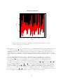
Conditional Predictive Ordinates (CPO) provide a way to assess the fit of the model to each site
individually (Lewis et al., 2014). The CPO for site i equals p(yi |y(i) ), where yi represents the data for site i
and y(i) represents all data except that for site i. CPOs are thus a form of cross-validation in which the
predictive distribution from all data except that from site i is used to predict the data observed at site i.
The CPO for site i is a measure of the success of the prediction, with high values meaning the data for site
i can be accurately predicted by a model based on all other data, and low values meaning that predictions
made from a model trained on all other data would often fail to correctly predict the data at the focal site.
Note that Phycas reports CPO values on the log scale, and thus these values are always negative (a
log(CPO) equal to 0.0 would be equivalent to a probability of 1.0, which would be seen only for a tree in
which all edge lengths are zero, or for a site having all missing data).
To get Phycas to calculate CPO values, perform an MCMC analysis using the cpo command rather than
the mcmc command. In reality, the mcmc command is still used to do the work, but calling cpo sets a few
mcmc variables before calling mcmc to begin the analysis. For example, one thing done in this initial setup is
to set mcmc.save sitelikes to True, which causes Phycas to save a (sometimes very large) file
containing the site log-likelihoods for every site for every sample. Because mcmc is doing all the
heavy-lifting, any mcmc settings you set will affect the outcome of a CPO analysis. Thus, if your alignment
10
comprises 2000 sites and you specify mcmc.ncycles to be 10000 and mcmc.sample every to be 10, then
the “sitelikes” file will contain 1000 rows and 2000 columns.
The name of the sitelikes file produced can be specified with mcmc.out.sitelikes setting (the file will be
named sitelikes.txt by default). You must used the command sump to summarize this file after the
analysis is finished. Set the setting sump.cpofile equal to a string specifying the name of the file of site
likelihoods produced by the mcmc command. You must specify sump.cpofile even if you did not modify
mcmc.out.sitelikes because, by default, the sump command does not even look for a file of site
likelihoods to summarize. In its summary, the sump command will use the harmonic mean of the site
likelihoods in one column of the sitelikes file as the estimate of the CPO for the site represented by that
column. (If you calculate these in some other program, such as Excel, note that the estimator equals the
log of the harmonic mean of the sampled site likelihoods, not the harmonic mean of the sampled site
log-likelihoods.) While the harmonic mean method is unstable for estimating the overall marginal
likelihood, it provides a stable and accurate method for estimating CPO values. The sump command will
not only output the overall log CPO (calculated as the sum over sites of the log CPO at each site), but will
generate a file containing the commands for generating a plot of log(CPO) vs. site in the software R.
The example <phycas install directory>/examples/cpo/cpo.py shows a complete example of a CPO
analysis. This example recreates Figure 4c in the Lewis et al. (2014) paper.
4
4.1
Tutorial
Warming up to Phycas
Phycas is an extension of Python, so to use it you must first start Python. In this section, you will
learn how to invoke Phycas commands from the Python command line. After you become familiar with
the basic commands, you will probably want to create a file containing the Phycas commands for a
particular analysis. Creating such a file (a Python script) makes it easier to remember exactly what
analyses you performed at some later time. (A Python script dedicated to a Phycas analysis will be
called a Phycas script.) If you want to redo an analysis, having the commands in a script file means you
do not have to type the majority of the commands over again. We will switch to using scripts in section 4.2
(“A basic analysis”).
First things first
Regardless of which platform (Windows, Mac, Linux) you are using, you must open a terminal window
(also known as a command prompt or console window in Windows) in order to use Phycas. At the
prompt, type python to invoke Python. Once Python has started, the prompt will change to three
greater-than symbols: >>>. At the >>> prompt, type from phycas import *, like this:
>>> from phycas import *
>>>
Phycas is an extension of Python, but you must import extensions in order for their capabilities to be
available. The import statement you typed means “import everything Phycas has to offer.”
Making life easier
If you find yourself using Phycas often, and thus end up typing from phycas import * over and over,
you should consider installing iPython. (This section is optional; if you do not want to install iPython at
11
this time, just skip this section and continue the tutorial at the next section 4.1 (entitled “Getting help”)
Once iPython is installed, create a default configuration profile as follows
ipython profile create
Now edit the ipython config.py mentioned in the output (look for “Generating default config file:”) and
replace
# lines of code to run at IPython startup.
c.InteractiveShellApp.exec_lines = []
with this
# lines of code to run at IPython startup.
c.InteractiveShellApp.exec_lines = ['from phycas import *']
Now, starting iPython will automatically import phycas:
$ ipython
Python 2.7.5 (default, Mar 9 2014, 22:15:05)
Type "copyright", "credits" or "license" for more information.
IPython 2.1.0 -- An enhanced Interactive Python.
?
-> Introduction and overview of IPython's features.
%quickref -> Quick reference.
help
-> Python's own help system.
object?
-> Details about 'object', use 'object??' for extra details.
release_version is True
/////////////////////////////
///// Welcome to Phycas /////
/////////////////////////////
Version 2.0.0
Phycas is written by Paul O. Lewis, Mark Holder and David Swofford
Phycas is distributed under the GNU Public License (see LICENSE file for more
information).
In [1]:
Note that in iPython the python prompt looks different (In [1]: instead of >>>). This manual will
continue using the standard python prompt, but everything else should work as advertised.
Getting help
Now type help at the Python prompt. This will display the following help message:
>>> help
Phycas Help
12
For Python Help use "python_help()"
Commands are invoked by following the name by () and then
hitting the RETURN key. Thus, to invoke the sumt command use:
sumt()
Commands (and almost everything else in python) are case-sensitive -- so
"Sumt" is _not_ the same thing as "sumt" In general, you should use the
lower case versions of the phycas command names.
The currently implemented Phycas commands are:
commands
cpo
gg
like
mcmc
model
randomtree
refdist
scriptgen
ss
sump
sumt
Use <command_name>.help to see the detailed help for each command. So,
sumt.help
will display the help information for the sumt command object.
Ordinarily, typing help will invoke the Python help system; however, after Phycas has been imported
into Python, typing help now invokes the Phycas help system. You can still access Python’s
interactive help by typing python help()1 . Hopefully, the output is self-explanatory, so let’s try what the
output of the help command suggests: obtaining help for a particular command. Type model.help at the
Python prompt (>>>):
>>> model.help
model
Defines a substitution model.
Available input options:
Attribute
Explanation
============================== ==============================================
edgelen_hyperparam
The current value of the edge length
hyperparameter - setting this currently has no
effect
edgelen_hyperprior
The prior distribution for the hyperparameter
that serves as the mean of an Exponential edge
length prior. If set to None, a nonhierarchical model will be used with respect
to edge lengths. Note that specifying an edge
length hyperprior will cause internal and
external edge length priors to be Exponential
distributions (regardless of what you assign
1 If you do try typing python help(), note that you can quit the Python help system (and return to using Phycas) by
typing quit at the help> prompt
13
to internal_edgelen_prior,
external_edgelen_prior or edgelen_prior).
.
.
.
state_freqs
The current values for the four base frequency
parameters
tree_length_prior
Use the Rannala, Zhu, and Yang (2012) tree
length distribution (if specified,
internal_edgelen_prior,
external_edgelen_prior, and edge_len will be
ignored). A reasonable default tree length
prior is TreeLengthDist(1.0, 0.1, 1.0, 1.0),
which makes tree length exponentially
distributed with mean and std. dev. 10 and
edge length fractions distributed according to
a flat Dirichlet
type
Can be 'jc', 'hky', 'gtr' or 'codon'
============================== ==============================================
(Note that I have replaced much of the output with a vertical ellipsis.) You will probably need to scroll up
to see all of the output of the model.help command. The output shows what model settings are available.
Thus, we see that model.type can be one of four things: ’jc’, ’hky’, ’gtr’ or ’codon’.
The output just generated shows us what settings are available, but what model is currently specified by
these settings? To see the current values of model settings, use the model.current command:
>>> model.current
Current model input settings:
Attribute
==============================
edgelen_hyperparam
edgelen_hyperprior
edgelen_prior
external_edgelen_prior
fix_edgelen_hyperparam
fix_edgelens
fix_freqs
fix_kappa
fix_omega
fix_pinvar
fix_relrates
fix_scaling_factor
fix_shape
gamma_shape
gamma_shape_prior
internal_edgelen_prior
kappa
kappa_prior
num_rates
omega
omega_prior
pinvar
pinvar_model
pinvar_prior
Current Value
==============================================
0.05
InverseGamma(2.10000, 0.90909)
None
Exponential(2.00000)
False
False
False
False
False
False
False
True
False
0.5
Exponential(1.00000)
Exponential(2.00000)
4.0
Exponential(1.00000)
1
0.05
Exponential(20.00000)
0.2
False
Beta(1.00000, 1.00000)
14
relrate_param_prior
relrate_prior
Exponential(1.00000)
Dirichlet((1.00000, 1.00000, 1.00000, 1.00000,
1.00000, 1.00000))
relrates
[1.0, 4.0, 1.0, 1.0, 4.0, 1.0]
scaling_factor
1.0
scaling_factor_prior
Exponential(1.00000)
state_freq_param_prior
Exponential(1.00000)
state_freq_prior
Dirichlet((1.00000, 1.00000, 1.00000,
1.00000))
state_freqs
[0.25, 0.25, 0.25, 0.25]
tree_length_prior
None
type
'hky'
============================== ==============================================
Now we can see that the current (default) model type is ’hky’. Suppose you wanted to use the GTR
model rather than the HKY model. You can do this by changing the model.type setting as follows:
>>> model.type = 'gtr'
>>> model.curr
Entering model.current (or the abbreviated version, model.curr) shows the list of current values,
allowing you to confirm that your change has been made.
The quotes around ’gtr’ are important. They indicate to Python that you are specifying a string (a
series of text characters) rather than the name of some other sort of object. If you typed gtr without the
quotes, Python would assume you are referring to a variable. Because it will (presumably) not find a
variable by that name, you will get the following error message if you forget the quotes:
>>> model.type = gtr
Error: name 'gtr' is not defined
Note that Python allows you use double-quotes or single-quotes to delimit strings – either will work to
tell Python that you mean a string rather than the name of a variable. Do not be confused by the subtle
differences in typesetting within this manual. In all cases you should use plain quotes in Python (not the
“back-tick” character or any special curved quote that is found in some word-processing programs).
The setting model.kappa prior specifies the prior probability distribution to use for the
transition/transversion rate ratio. Phycas defines several probability distributions for use as priors. In
this case, the current value of Exponential(1.00000) indicates that the κ parameter will be assigned
an exponential(1) prior distribution. See section 5.2 (p. 41) for a complete list of probability distributions
available within Phycas.
The setting model.relrates specifies the values of the six GTR relative rate parameters (also known as
exchangeability parameters). The square brackets around the value of the model.relrates parameter,
[1.0, 4.0, 1.0, 1.0, 4.0, 1.0], indicate that you should specify the six relative rate values as a
Python list. These should be specified in this order: A↔C, A↔G, A↔T, C↔G, C↔T, G↔T. The
model.relrates setting and others like it, such as model.kappa, model.state freqs,
model.gamma shape, and model.pinvar are used to set the starting values for an MCMC analysis (the
mcmc command) or to specify the values of parameters for calculating the likelihood (the like command).
The model.fix relrates command is used to specify whether the relative rates are to be allowed to vary
during an MCMC analysis (model.fix relrates=False) or are to be frozen at the values specified by
model.relrates (model.fix relrates=True). The values True and False are known to Python and
should not be surrounded by quotes (note also that case is important: typing true or TRUE will generate a
“not defined” error message from Python).
15
4.2
A basic analysis
The next task is to create a Phycas script containing the commands to carry out a basic MCMC analysis.
A Phycas script is a file containing Python source code that includes Phycas commands. When
submitted to the Python interpreter (a computer program), the commands in the script file are read and
executed.
Before proceeding...
Exit your current Python session by typing Ctrl-d (MacOS or Linux) or Ctrl-z (Windows® ).
Create a new, empty directory (a.k.a. folder) in which to experiment. It does not matter where this folder
is located, but before proceeding you must navigate into this directory from your terminal. (You can create
a new directory using the mkdir command (e.g. mkdir test), and change into that new directory using
the cd command (i.e. cd test).)
Using the scriptgen to create scripts
Start Python by typing python at the command prompt, then import Phycas using from phycas
import *. The scriptgen command makes it easy to create Phycas script files for doing common types
of analyses. Type the following to see the default settings for the scriptgen command:
>>> scriptgen.curr
Current scriptgen input settings:
Attribute
Current Value
============================== ==============================================
analysis
'mcmc'
datafile
'sample.nex'
model
'jc'
seed
0
============================== ==============================================
Current scriptgen output settings:
Attribute
Current Value
============================== ==============================================
out.level
OutFilter.NORMAL
out.script
out.script.prefix
out.script.mode
'runphycas.py'
'runphycas'
ADD_NUMBER
out.sampledata
out.sampledata.prefix
out.sampledata.mode
'sample.nex'
'sample'
ADD_NUMBER
The setting scriptgen.analysis is set to ’mcmc’, the setting scriptgen.datafile is set to
’sample.nex’, and the setting scriptgen.model is set to ’jc’. We will leave these at their default
settings, but let’s change scriptgen.seed to ’12345’ so that the analysis can be repeated exactly later
using this same pseudorandom number seed:
>>> scriptgen.seed = 12345
Let’s also change the setting scriptgen.out.script to ’basic.py’, then review the new settings:
16
>>> scriptgen.out.script = 'basic.py'
>>> scriptgen.curr
All that is left is to actually run scriptgen using these settings:
>>> scriptgen()
Script file was
The sample data
The sample data
Script file was
opened successfully
file was opened successfully
file was closed successfully
closed successfully
The line scriptgen() tells the scriptgen command to go ahead and create the script named basic.py
based on its current settings.
Open the newly-created basic.py file in a text editor (e.g. NotePad++ on Windows® or TextWrangler on
Mac). Verify that the following lines of Python code have been saved in this file by the scriptgen
command:
from phycas import *
setMasterSeed(12345)
# Set up JC model
model.type = 'jc'
# Assume no invariable sites
model.pinvar_model = False
# Assume rate homogeneity across sites
model.num_rates = 1
# Use independent exponential priors (mean 0.1) for each edge length parameter
model.edgelen_prior = Exponential(10.0)
model.edgelen_hyperprior = InverseGamma(2.10000, 0.90909)
mcmc.data_source = 'sample.nex'
# Conduct a Markov chain Monte Carlo (MCMC) analysis
# that samples from the posterior distribution
mcmc.ncycles = 10000
mcmc.burnin = 1000
mcmc.target_accept_rate = 0.3
mcmc.sample_every = 100
mcmc.report_every = 100
#mcmc.starting_tree_source = TreeCollection(newick='(1:.01,2:0.01,(3:0.01,4:0.01):0.01)')
#mcmc.starting_tree_source = TreeCollection(filename='nexustreefile.tre')
mcmc.fix_topology = False
mcmc.allow_polytomies = False
mcmc.bush_move_weight = 0
mcmc.ls_move_weight = 100
mcmc.out.log = 'mcmcoutput.txt'
mcmc.out.log.mode = REPLACE
mcmc.out.trees = 'trees.t'
mcmc.out.trees.mode = REPLACE
mcmc.out.params = 'params.p'
17
mcmc.out.params.mode = REPLACE
mcmc()
# Summarize the posterior distribution of model parameters
sump.file = 'params.p'
sump.skip = 1
sump.out.log.prefix = 'sump-log'
sump.out.log.mode = REPLACE
sump()
# Summarize the posterior distribution of tree topologies and clades
sumt.trees = 'trees.t'
sumt.skip = 1
sumt.tree_credible_prob = 0.95
sumt.save_splits_pdf = True
sumt.save_trees_pdf = True
sumt.out.log.prefix = 'sumt-log'
sumt.out.log.mode = REPLACE
sumt.out.trees.prefix = 'sumt-trees'
sumt.out.trees.mode = REPLACE
sumt.out.splits.prefix = 'sumt-splits'
sumt.out.splits.mode = REPLACE
sumt()
Line-by-line explanation
from phycas import *
N When you first start Python, it knows nothing about Phycas. You must import the functionality
provided by Phycas before any of the Phycas commands described in this manual will work. This first
line tells the Python interpreter to import everything (the asterisk symbol means “everything”) from the
phycas module. This line should start every Phycas script you create.2
setMasterSeed(12345)
N If the line above were left out of the script, you would obtain perfectly valid results, but the output
would be different each time you ran the script. Most of the time you would probably like to have the
option of later repeating an analysis exactly (for example, you might want to make the Phycas script used
to obtain the results for a published paper available to reviewers or the scientific community). To do this in
Phycas, the setMasterSeed command must be included. This command establishes the first in a long
sequence of pseudorandom numbers that Phycas will use for the stochastic aspects of its Markov chain
Monte Carlo analyses.
Pseudorandom numbers (as the name suggests) are not really random, but they behave for all intents and
purposes like random numbers. One difference between the numbers generated by Phycas’ pseudorandom
number generator and real random numbers is that a sequence of pseudorandom numbers is repeatable,
whereas sequences of true random numbers are not repeatable. To repeat a sequence of pseudorandom
numbers, you must start with the same pseudorandom nubmer seed, which should be a positive integer
(whole number). Here we’ve set the seed to the number 12345. The setMasterSeed command should
2 Unless you are using iPython and have configured it to always import Phycas upon startup (it doesn’t hurt to enter from
phycas import * again, however, so there is no reason to remove this line from automatically generated scripts).
18
come just after the from phycas import * command; it makes sense that if the master seed is set after
Phycas begins using pseudorandom numbers, then the results will differ from run to run.
# Set up JC model
model.type = 'jc'
# Assume no invariable sites
model.pinvar_model = False
# Assume rate homogeneity across sites
model.num_rates = 1
N These lines specify that the model should be a Jukes-Cantor (JC) model without rate heterogeneity. The
line model.pinvar model = False says to not allow the proportion of invariable sites to be estimated,
and the line model.num rates = 1 says to just use one rate category (using more than 1 rate category
automatically adds discrete gamma rate heterogeneity to the model).
# Use independent exponential priors (mean 0.1) for each edge length parameter
model.edgelen_prior = Exponential(10.0)
model.edgelen_hyperprior = InverseGamma(2.10000, 0.90909)
N These lines specify that the prior probability distribution for each individual edge length should an
Exponential(µ) distribution, where µ is a hyperparameter with an InverseGamma hyperprior. The 10
specified in model.edgelen prior = Exponential(10.0) serves to determine the initial value of
the hyperparameter µ. If we were to set model.edgelen hyperprior to None, the model would not use a
hyperparameter for the mean of the edge length prior distribution, and the 10 in this case would explicitly
determine the edge length prior distribution. Setting model.edgelen hyperprior to a valid probability
distribution establishes a hierarchical model in which the exponential prior mean is determined by a
hyperparameter, and model.edgelen hyperprior.is the (hyper)prior for that mean parameter. Note
that if a hyperprior is specified, then Phycas will always use an Exponential edge length prior distribution
(i.e. if model.edgelen hyperprior is defined, then model.edgelen prior must specify an Exponential
distribution, otherwise an error will be reported).
mcmc.data_source = 'sample.nex'
N This line specifies that the data should be read from the file named sample.nex, which should have
been created by the scriptgen command. In our case, sample.nex is in the same directory as this
script, but if it were in a different folder then you would need to specify a relative or absolute path to the
file3 . The file name is specified as a string, so be sure to surround the file name with single quotes so that
the Python interpreter will not complain.
mcmc.ncycles = 10000
N The setting mcmc.ncycles determines the length of the MCMC run. Cycles in Phycas are not the
same as generations in MrBayes. About two orders of magnitude fewer Phycas cycles are needed than
MrBayes generations, so a 10000 cycle Phycas run corresponds (roughly) to a 1,000,000 generation
MrBayes run. This does not mean that Phycas runs faster (or slower) than MrBayes; it simply means
that Phycas does more work during a single “cycle” than MrBayes does in one “generation.” In short,
Phycas attempts to update every non-edge-length parameter at least once during a cycle, and updates
3
For example, if the data file was in a directory named xyz at the same level as the directory containing the script, set
mcmc.data source to ’../xyz/sample.nex’
19
many (but not all) edge length parameters as well, whereas MrBayes chooses a parameter at random to
update in each of its generations.4
mcmc.burnin = 1000
mcmc.mcmc.target_accept_rate = 0.3
N The setting mcmc.burnin determines the length of the burn-in phase of the MCMC simulation. A
burn-in cycle is identical to any other cycle in Phycas except that (1) no samples are taken during the
burn-in phase and (2) updaters are autotuned during the burn-in but not during the later sampling phase
of MCMC. Autotuning is the process by which the updaters are tuned to have optimal efficiency. By
default, the slice width of the slice sampler (Neal, 2003) used by many parameter updaters (e.g. those
responsible for updating the gamma shape parameter, edge lengths and edge length hyperparameters, the
transition-transversion rate ratio, and the proportion of invariable sites) is adjusted every cycle during the
burn-in phase, and the tuning parameter of Metropolis-Hastings updaters (e.g. those responsible for
updating the tree topology, for scaling all edges in a tree simultaneously, and for updating all base
frequencies, codon frequencies, subset relative rates, or GTR exchangeabilities simultaneously) is adjusted
every cycle during the burn-in phase in an attempt to achieve the target acceptance rate specified by
mcmc.target accept rate using the method of Prokaj (2009). Some updaters may not be able to achieve
the target acceptance rate (especially true of the Larget-Simon tree topology updater), so you should not
be alarmed if not all updaters reach the goal. Slice samplers ignore mcmc.target accept rate because the
goal for them is to minimize the number of log-likelihood calculations, not to achieve a particular target
acceptance rate.
mcmc.sample_every = 100
N The setting mcmc.sample every determines how many cycles elapse before the tree and model
parameters are sampled. In this case, a sample is saved every 100 cycles, and the number of cycles is
10000, so a total of 100 trees (and 100 values from each model parameter) will be saved from this run.
mcmc.report_every = 100
N The setting mcmc.report every determines how many cycles elapse before a progress report is issued.
In this case, an update on the progress of the run will be issued every 100 cycles.
#mcmc.starting_tree_source = TreeCollection(newick='(1:.01,2:0.01,(3:0.01,4:0.01):0.01)')
N This line begins with a hash character (#), which causes Python (and hence Phycas) to ignore the
entire line. The scriptgen command placed this line in your file because you may wish to uncomment it
at some point if you decide to provide a starting tree description. If you do uncomment the line and
replace the newick tree description, be sure that the numbers in the tree description correspond to the
order in which taxa appear in the data file, and note that the tree description is entered as a string, so the
quotes before the beginning left parenthesis and after the ending parenthesis are necessary.
mcmc.fix_topology = False
N This line says the the tree topology is to be considered unknown and should be modified during the run.
If this is set to True, then you should supply a starting tree, otherwise Phycas will use a random starting
4 To compare the speed of MrBayes with Phycas, you should compare the time it takes, on average, to calculate the
likelihood, which is the most computationally expensive task either program performs. Phycas reports this average value at
the end of a run. MrBayes computes the likelihood roughly one time per generation if you specify mcmcp nrun=1 nchain=1.
Also, be sure to compare the two programs under the same model and on the same dataset and with the same computer!
20
tree topology, which is probably not what you want.
mcmc.allow_polytomies = False
N This line tells Phycas to only consider fully-resolved tree topologies. Setting mcmc.allow polytomies
to True will result in a reversible-jump MCMC analysis in which the chain proposes changes to the
number and size of polytomies in addition to the standard Larget-Simon LOCAL move, and the polytomy
prior described in Lewis et al. (2005) will be applied.
mcmc.bush_move_weight = 0
mcmc.ls_move_weight = 100
N These lines determine the number of times a Bush move or Larget-Simon LOCAL move are used during
each cycle. The Bush move proposes deletion or addition of edges in the tree. Deleting an edge creates (or
increases the size of ) a polytomy, while adding an edge removes (or reduces the size of) a polytomy. The
value specify is 0 because Setting mcmc.allow polytomies is False. If mcmc.allow polytomies were
changed to True, you might want to set both mcmc.bush move weight and mcmc.ls move weight to 50.
mcmc.out.log = 'mcmcoutput.txt'
N This line starts a log file, which captures all output sent to the console. Some consoles do not have a
large buffer, and it is possible to lose the beginning of the output if an analysis runs for a long time. Note
that the name of the log file must be in the form of a Python string: that is, failing to surround the file
name with quotes will result in an error.
mcmc.out.log.mode = REPLACE
N This line specifies the mode for the log file. The mode of any output file determines what happens if a
file by that name already exists. The default mode is ADD NUMBER, which creates a file by the same name
but with a number at the end. For example, if mcmcoutput.txt already exists, then the new log file would
be named mcmcoutput1.txt. If mcmcoutput1.txt already exists, then the new log file would be named
mcmcoutput2.txt, and so on. You can specify REPLACE (as we have done here) to replace any existing file
with the same name, or APPEND to add to the end of an existing file.
mcmc.out.trees = 'trees.t'
mcmc.out.trees.mode = REPLACE
N This line specifies that the trees sampled during the MCMC analysis will be saved to a file having the
name trees.t. If you preferred, you could have specified only the file name prefix using
mcmc.out.trees.prefix = ’trees’ and Phycas would add the extension .t to the end of the prefix
you specified. The mcmc.out.trees.mode command tells Phycas to simply replace the trees file if a
file by the name tree.t already exists.
mcmc.out.params = 'params.p'
mcmc.out.params.mode = REPLACE
N This line specifies that the parameters sampled during the MCMC analysis will be saved to a file having
the name params.p. The mcmc.out.trees.mode command tells Phycas to simply replace the
21
parameter file if a file by the name params.p already exists.
mcmc()
N This begins an MCMC analysis using defaults for everything except the settings that you modified. To
see what additional settings can be changed before calling the mcmc method, type mcmc.help (to see
explanations) or mcmc.current (to see current values) at the Python prompt.
Phycas provides the sump and sumt commands for summarizing parameter and tree files, respectively.
While analogous, Phycas’ sump and sumt commands differ somewhat from the corresponding MrBayes
commands. The final two sections of the basic.py tells Phycas to summarize the parameters and trees
sampled during the MCMC run. The MCMC analysis is performed when the mcmc() line is executed, so
we can assume (unless the run quit due to an error) that the files params.p and trees.t now exist.
# Summarize the posterior distribution of model parameters
sump.file = 'params.p'
sump.skip = 1
sump()
The setting sump.file specifies the name of the parameter file to analyze. The setting sump.skip is the
number of lines of parameter values to skip. This value should always be at least 1 because the first line in
the tree file represents the starting values, which do not represent a valid sample from the posterior
distribution. All statistics computed by the sump method are based on the number of sampled trees
remaining after the burn-in samples have been removed from consideration. For example, if there are 101
lines of sampled parameters in the input parameter file, and sump.skip is 1, all posterior probabilities will
be computed using 100 in the denominator (not 101).
sump.out.log.prefix = 'sump-log'
sump.out.log.mode = REPLACE
N These lines specify the name of the log file to use in saving the output of the sump command.
sump()
N Calling the sump command begins the analysis of the input parameter file. Output is generated by this
method summarizing the parameters sampled. The parameter summary table includes the following
information:
param The name of the parameter
n The number of valid samples of this parameter obtained from the parameter file
autocorr A measure of autocorrelation (close to 0 is best, and negative values are fine as long as they are
not large in magnitude)
ess The effective sample size estimated from the autocorrelation (equal to n if autocorrelation is 0, less
than n if autocorrelation is positive)
lower 95% The lower boundary of the 95% credible interval for this parameter
upper 95% The upper boundary of the 95% credible interval for this parameter
min The minimum value recorded for this parameter
22
max The maximum value recorded for this parameter
mean The marginal posterior mean for this parameter
stddev The marginal posterior standard deviation for this parameter
A word about autocorrelation is in order. If MCMC samples are highly autocorrelated, then you effectively
have a smaller sample size than you might have thought given the actual sample size. To see this, imagine
a perfectly autocorrelated sample in which every sampled value is exactly the same. In this case, you really
only have a sample size of 1, even though Phycas might have saved 2000 values. The effective sample size
is computed from the autocorrelation. The effective sample size would thus be 1 if samples were perfectly
autocorrelated.
# Summarize the posterior distribution of tree topologies and clades
sumt.trees = 'trees.t'
sumt.skip = 1
N The setting sumt.trees specifies the name of the tree file to analyze. Note that you need not run the
sumt command from the same script that starts the MCMC analysis; all this command needs is the name
of an existing tree file, and thus it can be run at any time. The setting sumt.skip is the number of
sampled tree topologies to skip. As with the sump.skip setting, this value should always be at least 1
because the first tree in the tree file is the starting tree, which is never a valid sample from the posterior
distribution. All statistics computed by the sumt method are based on the number of sampled trees
remaining after the burn-in trees have been removed from consideration. For example, if there are 101 trees
in the input tree file, and sumt.skip is 1, all posterior probabilities will be computed using 100 in the
denominator (not 101).
sumt.tree_credible_prob = 0.95
sumt.save_splits_pdf = True
sumt.save_trees_pdf = True
N The sumt.tree credible prob setting determines the proportion of the posterior distribution included
in the credible set of tree topologies. Tree topologies stored are ranked from highest to lowest marginal
posterior probability, and tree topologies are then included in the credible set (starting with the one having
the highest marginal posterior probability) until the cumulative marginal posterior probability exceeds the
value specified by sumt.tree credible prob. If the data are quite informative, it is possible that just one
tree topology is included in the credible set; however, if the data have low information content relevant to
estimating tree topology, the number of trees in the 95% credible set could be quite large.
If a large number of trees are included in the credible set, the size of the PDF files generated could get
quite huge. The settings sumt.save splits pdf and sumt.save trees pdf can be set to False to avoid
producing the PDF files. You may wish to play it safe and always instruct Phycas to avoid producing
PDF files the first time you run sumt for a particular analysis. You can always run sumt again later, this
time setting sumt.save splits pdf and sumt.save trees pdf to True.
sumt.out.log.prefix = 'sumt-log'
sumt.out.log.mode = REPLACE
N These lines specify the name of the log file to use in saving the output of the sumt command.
sumt.out.trees.prefix = 'sumt-trees'
sumt.out.trees.mode = REPLACE
N The setting sumt.out.trees.prefix specifies the prefix used to create (output) file names for a tree
file (prefix + .tre) and a pdf file (prefix + .pdf). Both files will contain the same trees, but the trees in the
23
pdf file are graphically represented whereas those in the tree file are in the form of newick (nested
parentheses) tree descriptions. The first tree in each file is the 50% majority-rule consensus tree (see
Holder, Sukumaran, and Lewis, 2008, for why the majority rule tree is a good summary of the posterior
distribution), followed by all distinct tree topologies sampled during the course of the MCMC analysis that
are in the specified credible set (the 95% credible set by default). The graphical versions in the pdf file
have edge lengths drawn proportional to their posterior means and with posterior probability support
values shown above each edge. With the exception of the majority rule consensus tree, the titles of trees
reflect their frequency in the sample. The REPLACE mode tells Phycas to overwrite (without asking!)
sumt-trees.pdf and sumt-trees.tre if either file happens to already exist.
sumt.out.splits.prefix = 'sumt-splits'
sumt.out.splits.mode = REPLACE
N The setting sumt.out.splits.prefix specifies the prefix used to create a file name for a pdf file
containing two plots. The first plot in the file is similar to an AWTY (Nylander et al., 2008) cumulative
plot. It shows the split posterior probability calculated at evenly-spaced points throughout the MCMC run
(as if the MCMC run were stopped and split posteriors computed at that point in the run). This kind of
plot gives you information about whether the Markov chain converged with respect to split posteriors.
(Often, when plots of log-likelihoods or model parameters show apparent convergence, split posteriors are
still changing, making this type of plot a better indicator of convergence.) This first plot is not identical to
an AWTY cumulative plot. The most striking difference is the fact that the lines plotted all originate at
zero (AWTY does not plot these initial segments). Also, in AWTY the x-axis is labeled in terms of
generations, whereas the Phycas equivalent labels the x-axis in terms of cumulative sample size.
The second plot in this file shows split sojourns. A split sojourn is a sequence of successive samples in
which the split is present in the sampled tree, preceded and followed by an absence of the split. The
number and duration of split sojourns gives an indication of how well the Markov chain is mixing, and this
plot shows the results graphically. Neither plot in this file shows results for trivial splits (the split
separating a single taxon from all other taxa; such splits are always present and are thus guaranteed to
have split posterior 1.0) or for splits that were present in every sample (these are not useful from the
standpoint of assessing convergence or mixing, except that poor mixing might be indicated if very few splits
are plotted). See Lewis and Lewis (2005) for an example of the use of split sojourns to assess convergence.
sumt()
N The sumt method call begins the analysis of the input tree file. Besides the three files produced
containing trees and plots, output is generated by this method summarizing the splits and tree topologies
discovered. The split summary table includes the following information:
split The index of the split
pattern A sequence of hyphens and asterisks indicating which taxa are on either side of the split. The
patterns are normalized so that the first taxon is always represented by a hyphen.
freq. The number of trees in which the split was found
prob. The frequency of the split in the sample divided by the total number of trees sampled
weight The posterior mean edge length of the split, obtained by averaging the edge length associated with
the split over all sampled trees in which the split was found
s0 This is the first sample in which the split appeared. The minimum possible value of this quantity is 1,
and the maximum is the number of trees sampled.
24
sk This is the last sample in which the split appeared. The minimum possible value of this quantity is 1,
and the maximum is the number of trees sampled.
k This is the number of sojourns made by the split. A sojourn is a sequence of sampled trees in which the
split appears, preceded and followed by a sampled tree lacking that split.
The tree topology summary table includes the following information:
topology The index of the topology
freq. The number of trees in which the topology was found
TL The posterior mean tree length associated with a topology, obtained by averaging the tree length
associated with the topology over all sampled trees having that topology
s0 This is the first sample in which the tree topology appeared. The minimum possible value of this
quantity is 1, and the maximum is the number of trees sampled.
sk This is the last sample in which the tree topology appeared. The minimum possible value of this
quantity is 1, and the maximum is the number of trees sampled.
k This is the number of sojourns made by the tree topology. A sojourn is a sequence of sampled trees in
which the topology appears, preceded and followed by a sampled tree lacking that topology.
prob. The frequency of the topology in the sample divided by the total number of trees sampled
cum The cumulative posterior probability over all tree topologies sorted from most to least probable. This
column aids in finding credible sets of trees. For example, the 95% credible set of tree topologies
would be all those above (and including) the first one having a cumulative probability at least 0.95.
Invoking Phycas commands
For Phycas commands such as mcmc, adding the parentheses after the name of the command generally
serves to start the analysis that the command implements. There are exceptions to this rule. For example,
the “action” associated with the model command is simply the creation of a copy of the model for
purposes of saving the current model settings. Thus, you could issue the following command:
m1 = model()
to save the current model settings to a variable named m15 . Why would you want to save your model? It
is necessary to save the model if you are planning to partition your data because the partitioning
commands require you to specify a model (e.g. “m1”) along with the set of sites to which that model
applies. You will read more about partitioning in section 4.3 on page 27. For this example, we do not need
to save the model because we are using just one model for all sites (i.e. an unpartitioned analysis).
The randomtree() invocation returns a TreeCollection that holds a set of simulated trees and is
another example of a command that does not produce visible output.
5 The name “m1” here is arbitrary, but you should be careful to avoid using names that are identical to those Phycas or
Python uses. For example, if you named your model “mcmc”, then you would lose the ability to perform an MCMC analysis
because you have redefined the name “mcmc” to mean something else!
25
Running basic.py
To execute the basic.py script you just created, open a console window, navigate6 to the directory
containing the script and type the following at the command prompt:
python basic.py
While Phycas is running, it will provide progress reports every mcmc.report every update cycles and
periodic “Updater diagnostics” reports such as the following:
cycle = 6200, lnL = -343.90083 (4 seconds remaining)
cycle = 6300, lnL = -344.46491 (4 seconds remaining)
Updater diagnostics (* = slice sampler):
accepted 66.9% of 3200 attempts (tree_scaler)
accepted 36.0% of 320000 attempts (larget_simon_local)
* efficiency = 16.5%, mode=0.15199 (edgelen_hyper)
cycle = 6400, lnL = -344.72761 (3 seconds remaining)
cycle = 6500, lnL = -342.36245 (3 seconds remaining)
The updater diagnostics report above says that Phycas has thus far attempted to rescale the tree 3200
times and accepted 66.9% of those attempts, and has attempted 320000 Larget-Simon LOCAL move
(without a molecular clock) proposals (Larget and Simon, 1999) and accepted 36.0% of them. Both of
these are Metropolis-Hastings proposals (Metropolis et al., 1953; Hastings, 1970). Many parameter updates
in Phycas use slice sampling (Neal, 2003) instead of Metropolis-Hastings. These slice-sampling updates
are indicated by an asterisk (∗) and the efficiency rather than the acceptance rate is what is reported. The
efficiency is the inverse of the number of likelihood calculations needed before a sample is returned. The
“mode” reported is the previously-sampled value of the parameter associated with the highest posterior
density thus far. It is not the mode of the marginal posterior distribution of the parameter, which would be
much more difficult to estimate. The mode reported here is intended merely to provide a rough idea of the
best current value of the parameter.
Note that updater diagnostics reports are generated at 100, 200, 300, etc., cycles. The value 100 comes
from mcmc.report efficiency every.
Output of basic.py
The program should run for a few minutes, after which you should find the following files in the same
directory as basic.py and sample.nex:
mcmcoutput.txt This file contains a copy of the output you saw scrolling by as the analysis ran. This file
was generated by the mcmc command.
params.p Each line of this file represents a sample of parameter values from the posterior distribution
(except for tree and edge lengths).
trees.t Each line of this file represents a tree (with edge lengths) sampled from the posterior distribution.
6 If you are using an older version of Windows® , we suggest you read section 2.1, where a registry trick is described that
enables you to open a console window positioned at a particular directory by right-clicking the name of the folder in an Explorer
or My Computer window. This saves having to navigate to the directory after opening the console window, which can be a
very tedious and time consuming operation if the directory in which your script resides is nested deep inside your file system.
Windows 7 already has this capability built in: use shift-right-click to see the “Open command window here” menu item.
26
sump-log.txt This file contains a copy of the output generated by the sump command.
sumt-log.txt This file contains a copy of the output generated by the sumt command.
sumt-splits.pdf This 2 page pdf file contains an AWTY-style plot showing the split posteriors through
time and a sojourn plot showing when the most important splits appeared and disappeared through
time.
sumt-trees.pdf This pdf file contains a graphical representation of the majority-rule consensus tree and
each tree in the credible set.
sumt-trees.tre This NEXUS tree file contains the majority-rule consensus tree and each tree in the
credible set.
4.3
Defining a partition model
This section describes partitioning, which is dividing your data set into subsets of sites and applying a
separate model to each subset. The noun partition means “wall” and the verb to partition refers to the
act of dividing something into parts (mutually-exclusive subsets). This accords with mathematical usage of
the term, but differs from common usage, where the term partition is treated as being synonymous with
subset (i.e. one room as opposed to the wall dividing up a space into separate rooms). This manual uses
partition to mean “a particular way of dividing sites into mutually exclusive subsets” and uses subset to
refer to the subsets of sites created by the partition.
To create a partition model in Phycas, you first define models for all subsets and then apply the models
to the appropriate sets of sites. Phycas always treats tree topology and edge lengths as (to use MrBayes’
terminology) “linked” across partition subsets (meaning that one tree topology and set of edge lengths
applies to all subsets), and always treats all other parameters as “unlinked” (these parameter values apply
to just one subset of sites). There is no way to tell Phycas to unlink edge links, and likewise there is no
way to tell it to use the same value of the gamma shape parameter for two different partition subsets. To
create an unpartitioned model, simply change the settings on the current model object (as we did in the
previous section) and, by default, that model will be applied to all sites.
I will use the following specification to illustrate how to set up a partitioned model and then you will be
given the chance to apply it to a real protein-coding gene set. The model that we will set up separates
first, second and third codon positions. You will apply a separate K80+G model to the first and second
codon positions and an HKY+G model to third positions.
The partition.py script
Create a new, empty folder and copy the file green.nex into it. The file green.nex can be found in your
Phycas installation directory at the location phycas/tests/data/green.nex. If you did not save the original
phycas folder that you unpacked after downloading, ask Python to show you where the phycas folder was
installed:
>>> import site
>>> print site.getsitepackages()
The output should include the full path to a directory named site-packages. The installed phycas folder will
be in that directory.
Ensure that you are in the folder containing green.nex, start Python and import Phycas, then use the
following scriptgen settings to create a Phycas script named partition.py:
27
>>>
>>>
>>>
>>>
scriptgen.model='hky+g'
scriptgen.datafile='green.nex'
scriptgen.out.script='partition.py'
scriptgen()
Open the new partition.py file in your favorite text editor. Add the two line indicated below to the section
starting with the comment # Set up HKY model:
# Set up HKY model
model.type = 'hky'
model.state_freqs = [0.25, 0.25, 0.25, 0.25] # add this line
model.fix_freqs = True
# add this line
model.kappa_prior = Exponential(1.0)
model.state_freq_prior = Dirichlet((1.0, 1.0, 1.0, 1.0))
The two lines added convert an HKY model into a K80 (also known as K2P) model by forcing the state
frequencies to be equal. You might be tempted to comment out the line specifying the
model.state freq prior because the base frequencies are now fixed and thus do not need a prior, but
please leave it in: we will use this setting later so commenting it out here will just necessitate adding it
back in later (prior settings are ignored if they are not needed).
Just before the line model.data source = ’green.nex’ (i.e. after the last line making changes to
model), add the following lines:
# Save the K80+G model
m1 = model()
m2 = model()
The K80+G model we have just established is first copied into two variables, m1 and m2. These models
will be used for the first and second codon position sites.
Now add lines just after those above to create the HKY+G model that will be used for third codon
position sites:
# Set up and save the HKY+G model
model.fix_freqs = False
m3 = model()
The current model differs from HKY+G only in the fact that the state frequencies are fixed. Before saving
the model again into the variable m3, we thus need to set model.fix freqs to False.
Add three more lines to specify which sites will belong to each of the three subsets:
first = subset(1, 1296, 3)
second = subset(2, 1296, 3)
third = subset(3, 1296, 3)
The three arguments to subset are the starting site, the ending site, and the stride (if currently at site i,
the next site will be i+stride). The variable names first, second and third are arbitrary variable
names. You might prefer first codon pos, second codon pos, and third codon pos. You are free
to use whatever names you like as long as they are valid Python variable names. (The same is true for
m1, m2, and m3.)
Finally, tell Phycas which models go with which subsets:
28
# Define partition subsets
partition.addSubset(first, m1, 'first')
partition.addSubset(second, m2, 'second')
partition.addSubset(third, m3, 'third')
partition()
For example, the first partition.addSubset command assigns the model stored in m1 to the subset
stored in first. The final partition() freezes the partition, telling Phycas that you are finished
modifying it. Phycas uses this opportunity to perform some sanity checks on your partition scheme and
will let you know if, for example, you’ve left out some sites or if your subsets are not mutually exclusive.
Running partition.py
Run the partition.py in Python as described for basic.py (see section 4.2 on page 26).
Output of partition.py
After the analysis has finished, you should find the following files:
mcmcoutput.txt This file contains a copy of the output you saw scrolling by as the analysis ran. This file
was generated by the mcmc command.
params.p Each line of this file represents a sample of parameter values from the posterior distribution
(except for tree and edge lengths). This file was generated by the mcmc command.
trees.t Each line of this file represents a tree (with edge lengths) sampled from the posterior distribution.
This file was generated by the mcmc command.
sump-log.txt This file contains a copy of the output generated by the sump command.
sumt-log.txt This file contains a copy of the output generated by the sumt command.
sumt-splits.pdf This 2 page pdf file contains an AWTY-style plot showing the split posteriors through
time and a sojourn plot showing when the most important splits appeared and disappeared through
time. This file was generated by the sumt command.
sumt-trees.pdf This pdf file contains a graphical representation of the majority-rule consensus tree and
each tree in the credible set. This file was generated by the sumt command.
sumt-trees.tre This NEXUS tree file contains the majority-rule consensus tree and each tree in the
credible set. This file was generated by the sumt command.
If you examine the params.p file, you will find that the parameters have numerical prefixes indicating the
subset model to which they belong. For example, 3 kappa is the transition/transversion rate ratio for
model m3, which was applied to the subset third. You will also see parameters named 1 subset rate,
2 subset rate and 3 subset rate. These are the relative rates at which each subset of sites evolves.
For example, the sump-log.txt file reveals that the posterior mean relative rate of third position sites
(3 subset rate) is 2.43460 while that for second position sites (2 subset rate) is only 0.13676, so
third position sites evolve, on average, almost 18 times faster than second position sites in this data set.
29
4.4
Estimating marginal likelihoods
The stepping-stone method was described earlier (see section 3.3 on page 8). In this part of the tutorial,
you will use the scriptgen command to create a Phycas script that carries out a stepping-stone analysis.
The steppingstone.py script
To perform a steppingstone analysis, create a new folder, copy green.nex into it, start Python inside the
new folder, import Phycas, and use the scriptgen command as illustrated below to create a Phycas
script named steppingstone.py:
>>>
>>>
>>>
>>>
>>>
scriptgen.analysis = 'ss'
scriptgen.datafile = 'green.nex'
scriptgen.model = 'gtr+i+g'
scriptgen.out.script = 'steppingstone.py'
scriptgen()
Running steppingstone.py
Run the steppingstone.py in Python as described for basic.py (see section 4.2 on page 26). While it is
running, read the line-by-line explanation below.
Line-by-line explanation
Most parts of this script have been described in previous sections, so this section will concentrate on
aspects of the script that are important for stepping-stone analyses.
# Estimate the marginal likelihood using the Generalized Stepping-stone (GSS) method
# Estimate the reference distribution to use with Generalized SS
refdist.skip = 1
refdist.params = 'params.p'
refdist.trees = 'trees.t'
refdist.out.refdistfile = 'refdist.txt'
refdist.out.refdistfile.mode = REPLACE
refdist()
N This section appears after the line mcmc(). A short MCMC analysis has been conducted, as usual
exploring the posterior distribution, and the purpose of this section is to summarize the posterior
distribution and generate the reference distribution that will be used in the stepping-stone analysis. The
settings refdist.params and refdist.trees specify the parameter and tree files, respectively, that were
generated by the previous MCMC analysis. The setting refdist.skip is set to 1 to skip the starting
values in both the parameter and tree file. The refdist.refdistfile determines the name of the
reference distribution file that will be generated, and the refdist.refdistfile.mode setting says to
replace this file if one by that name already exists. Finally, refdist() causes the refdist.txt file to be
30
created.
# Choose different output file names to avoid overwriting the
# ones used for the reference distribution
mcmc.out.log = 'ss-output.txt'
mcmc.out.log.mode = REPLACE
mcmc.out.trees = 'ss-trees.t'
mcmc.out.trees.mode = REPLACE
mcmc.out.params = 'ss-params.p'
mcmc.out.params.mode = REPLACE
N These commands are necessary because we are just about to conduct a new MCMC analysis. If these
lines were absent, the log, parameter and tree files generated by this new MCMC analysis would overwrite
the ones created by the first MCMC analysis (the one used to create the reference distribution). Setting
new names simply allows us to keep all the files and avoid possible confusion later about which MCMC
analysis generated them.
# Set up and run the ss command (this will make use of many mcmc settings)
ss.nstones = 20
ss.ncycles = 500
N The ss command uses the mcmc command to do almost all of its work. Hence, many of the settings that
affect a stepping-stone analysis are actually mcmc settings. The setting mcmc.ncycles specifies the number
of parameter update cycles devoted to each beta value visited. Note that this is the number of cycles per
beta value. If you specified ss.nbetavals to be 11 and mcmc.ncycles to be 1000, then the total number
of cycles would be 11 times 1000, or 11000 cycles.
This example uses 20 beta values (ss.nstones), but is this enough? Generally the more stepping stones
(i.e. beta values) used, the better the estimate will be, but the quality of the estimate also depends on the
quality of the reference distribution. If the reference distribution approximates the posterior well, then
fewer beta values are needed (and fewer samples per beta value are needed). If the reference distribution
exactly equals the posterior, then only a single sample from the reference distribution (beta = 0.0) would
be needed to determine the marginal likelihood exactly! (This utopia is never achievable because if one
actually knew the posterior distribution exactly, then one would also know the normalizing constant
exactly and hence you would not need to estimate it!) In practice, it probably makes sense to start with,
say, 20 β values, and a reasonable number (e.g. 500) cycles per β value. Then do another run, doubling
both values. If this makes a big difference, then probably the first run was not long enough (and perhaps
the second run too!).
ss.sample_every = 1
ss.report_every = 100
N Normally, the mcmc.sample every setting governs the degree of thinning performed. Thinning involves
ignoring some sampled parameter values in order to decrease autocorrelation or to avoid an excessive file
size. In principle, there is no reason to thin other than to keep the size of the parameter file small because
one could alway thin out the samples at a later time. Because we are not worried about the size of the
parameter file here, this line tells Phycas to save every sample (i.e. don’t thin; sample parameter values
every cycle).
ss.refdist_is_prior = False
ss.refdistfile = 'refdist.txt'
N The setting ss.refdist is prior is set to False because we want to use a reference distribution that
31
approximates the posterior for efficiency. The setting ss.refdistfile specifies the reference distribution
file that was created previously by the refdist command.
ss.shape1 = 1.000000
ss.shape2 = 1.000000
N The settings ss.shape1 and ss.shape2 determine how the β values are distributed on the interval from
0 to 1. If, as here, both are set to 1, the β values will be evenly distributed. If we had set
ss.refdist is prior to True, it would be better to choose ss.shape1 to be, say, 0.3, which would
place more β values near 0. When the prior is used as the reference distribution, there is a sharp change in
the value of the power posterior as β approaches 0, and both SS and TI are less biased if β values are
concentrated in this region of rapid change. See Xie et al. (2010) and Lepage et al. (2007) for more
in-depth explanations.
ss()
N This command starts the analysis. It essentially causes the mcmc command to be run for each β value
visited.
sump.out.log = 'ss.sump.log'
sump.out.log.mode = REPLACE
N The sump.out.log setting specifies the name of the file that will hold the output of the sump command.
Note that you must include the sump command because the ss command only carries out the MCMC
analysis; it is the sump command that actually computes the estimate of the marginal likelihood.
Output of steppingstone.py
The file ss-sump-log.txt contains the output of interest from this analysis. This file has three sections
labeled, respectively, Autocorrelations, Effective and actual sample sizes, and Marginal likelihood estimate.
The first and second sections are related, for it is the autocorrelations that determine the effective sample
sizes. You will note that the first line of the Effective sample sizes section (after the header line showing
the β values) provides the actual sample sizes. This is the number of times parameter values were saved
while the MCMC analysis was exploring a particular β value. The other rows in this table provide effective
sample sizes. Note the last column (for β = 0). The effective sample sizes in this column are often larger
than the actual sample size. What’s up with that? If there is zero autocorrelation, then the effective
sample sizes will hover around the actual sample size. If the autocorrelation is negative, then the effective
sample size will be larger than the actual sample size. When β = 0, Phycas is sampling directly from
standard probability distributions and zero autocorrelation is expected in this case. Even though zero
autocorrelation is expected, some parameters will have slightly negative autocorrelations and others will
have slightly higher autocorrelations. This is normal, and explains why some effective sample sizes are
greater than the actual sample size for this column.
The last section provides some information about each of the ratios (stepping stones) that it estimated in
the process of estimating the marginal likelihood. The first column (labeled b (k-1)) is the power (i.e.
value of β) used for the distribution being sampled. You will note that β = 1 (the posterior distribution) is
absent. This is because the samples taken from the posterior are used as burn-in, not for estimating the
individual ratios in the stepping-stone method. The column labeled beta incr shows the difference
between the current β value and the previous one. For the (default) generalized stepping-stone method,
these β increments should all be the same. The column labeled n provides the number of sample used for
32
that particular ratio. The column labeled lnRk is the log of the ratio of normalizing constants
corresponding to one stepping stone ratio. The product of the individual ratios equals the estimate of the
marginal likelihood. The last column, labeled lnR(cum) provides the running sum of the individual lnRk
values. The final estimate of the log of the marginal likelihood is provided at the bottom of the file.
4.5
Conditional Predictive Ordinates
Conditional Predictive Ordinates (CPO) was described earlier (see section 3.4 on page 10). In this part of
the tutorial, you will use the scriptgen command to create a Phycas script that carries out a CPO
analysis.
The cpo.py script
To perform a CPO analysis, create a new folder, copy green.nex into it, start Python inside the new
folder, import Phycas, and use the scriptgen command as illustrated below to create a Phycas script
named cpo.py:
>>>
>>>
>>>
>>>
>>>
scriptgen.analysis = 'cpo'
scriptgen.datafile = 'green.nex'
scriptgen.model = 'gtr+i+g'
scriptgen.out.script = 'cpo.py'
scriptgen()
Running cpo.py
Run the cpo.py in Python as described for basic.py (see section 4.2 on page 26). While it is running, read
the line-by-line explanation below.
Line-by-line explanation
Only the parts of of cpo.py that have not been previously described will be discussed below.
#mcmc()
# Using MCMC setup above, compute conditional predictive ordinates (CPO) for each site and for the en
cpo.out.sitelike.prefix = 'sitelikes'
cpo()
N There is an mcmc command in the file generated by scriptgen, but it is commented out. When
performing a CPO analysis, use the cpo command instead of the mcmc command to perform the MCMC
analysis. The cpo command is similar to the ss command in that it uses the machinery behind the mcmc
command to do almost all of the work, and thus effectively all that cpo really does is set up the mcmc
command so that it saves a file containing site log-likelihoods for every site every time parameters and the
tree are sampled. The snippet above shows how you can modify the name of this site log-likelihood file if
you wish. If you change just the prefix, as is done in the script generated by scriptgen, the extension .txt
will be appended. Alternatively, you could specify the entire name (prefix and extension) of the site
33
log-likelihood file using cpo.out.sitelike = ’sitelikes.txt’.
# Run sump command to summarize CPO values saved during MCMC
sump.file = 'params.p'
sump.skip = 1
sump.cpofile = 'sitelikes.txt'
sump.cpo_cutoff = 0.1
sump.out.log.prefix = 'sump-log'
sump.out.log.mode = REPLACE
sump()
N Note that the cpo command results in an MCMC analysis that saves a site log-likelihood file; it does not
actually estimate the CPO for any site! To do that, you need to run the sump command after the MCMC
analysis is finished, specifying the name of the site log-likelihood file in the sump.cpofile setting:
Output of cpo.py
The sump command will produce three files: cpoplot.R, cpoinfo.txt, and sump-log.txt. The cpoplot.R can be
used to create a plot of log(CPO) values for every site using the rscript script provided with R:
rscript cpoplot.R
The resulting plot is shown in Figure 1. The impulses colored red correspond to log(CPO) values that are
lower than the user-defined cutoff specified by sump.cpo cutoff, which in this example is 0.1 (i.e. the
worst 10% of sites according to CPO are colored red). While the plot provides a graphical depiction, it is
difficult to determine from the plot which sites are actually the ones colored red.
34
The cpoinfo.txt file provides two ways to find out which sites are in this lowest 10% category. First, near
the top of the file is a mask: a series of dashes and asterisks, one for every site, that can be copied and
pasted above the alignment in the data file. The sites in the lowest sump.cpo cutoff fraction are
indicated by the asterisks (∗). In the example below, I have deleted most of the mask, replacing the middle
part with ellipses that are absent in the actual mask:
BEGIN_MASK
---------*----------------*--*--*---*-*-----------*--------- ... -*------**END_MASK
The cpoinfo.txt file also contains a large table of log(CPO) values, one for each site, along with the data
subset to which that site belongs (only useful if you have partitioned the data) and a column indicating
whether the site has a CPO value in the lowest 10% of sites:
BEGIN_LOG_CPO_TABLE
site
log(CPO)
1
-1.66349
2
-1.66349
3
-1.66349
4
-1.96609
5
-1.66349
.
.
.
1295
-13.44352
1296
-9.16329
END_LOG_CPO_TABLE
subset
default
default
default
default
default
worst
0
0
0
0
0
default
default
1
0
(The BEGIN LOG CPO TABLE and END LOG CPO TABLE markers are provided to make it easy to extract
just this portion of the file using a regular expression.)
Finally, the sump-log.txt file contains the LPML (Log PseudoMarginal Likelihood) estimate, which is
simply the sum over all sites of the log(CPO). The LPML value can be used as an overall measure of model
performance and compared among different models in much the same way the marginal likelihood is used.
In this case, the LPML provides an overall measure of how well the model can predict the very data used
for fitting.
4.6
Polytomy analyses
Unlike most other programs for Bayesian phylogenetic inference, Phycas can be set up to allow its Markov
chain to visit tree topologies containing polytomies. In the most extreme case, Phycas could even spend
time on the star tree (i.e. a tree with only one internal node). The reasons one might want to allow
polytomous tree topologies to be assigned posterior probability mass are outlined in Lewis, Holder, and
Holsinger (2005). P4 (written by Peter Foster) also has the option of allowing polytomies. To convert an
existing Phycas script into one that allows polytomies, you need add the following 5 lines:
mcmc.allow_polytomies
mcmc.polytomy_prior =
mcmc.topo_prior_C
mcmc.bush_move_weight
mcmc.ls_move_weight =
= True
True
= exp(1.0)
= 50
50
35
−10
−15
CPO
−5
Overall CPO = −6565.47678
0
200
400
600
800
1000
1200
Site
Figure 1: The plot obtained by processing the cpoplot.R file produced by the cpo.py script
generated in section 4.5 of the tutorial.
The setting mcmc.allow polytomies, when set to True, tells Phycas that you wish for unresolved trees
to be visited in addition to fully-resolved trees. Unresolved trees are tree topologies with at least one
polytomy (an internal node with at least four connecting edges). A fully-resolved unrooted tree has
exactly three edges connecting to each internal node. The next two lines determine the kind of topology
prior you wish to use. There are two major possibilities: (1) a polytomy prior and (2) a prior on resolution
class.
The first (polytomy prior) is the easiest to understand, is the one implied by the command
mcmc.polytomy prior = True, and is the only one we will use in the following exercises. In the
polytomy prior, the relative prior probability of a tree with n internal nodes differs from the prior
probability of a tree with n + 1 internal nodes by the factor mcmc.topo prior C. If mcmc.topo prior C is
set equal to 1.0, then every tree topology, regardless of the number of internal nodes, would have the same
prior probability. Setting mcmc.topo prior C to a value greater than 1 favors less-resolved trees. If we
used the command mcmc.topo prior C = exp(1.0), then the factor used would be e1 (approximately
2.718), and a fully-resolved tree would need to have a likelihood 1 unit higher (on the log scale) to be
favored over a tree with one fewer internal node (and hence 1 fewer edge). To push the bar even higher,
you could set mcmc.topo prior C = exp(2.0), which sets the factor to e2 and requires a more-resolved
tree to be higher by 2 log-likelihood units to equal a tree with one more polytomy.
36
You might ask “Why should the prior favor less-resolved trees?” If you are tempted to perform a
polytomy-friendly analysis in the first place, it is probably because you fear that a false clade will receive
undue support. In such situations, you may prefer to be conservative, not only allowing polytomous trees
into the analysis but actually making it extra hard for a false clade to receive high support. We have found
that even a prior that strongly favors polytomies will be effectively defeated by the likelihood if there is any
sign at all that substitutions have occurred on an edge. For example, one sees polytomies in trees for data
simulated under a very low rate of substitution on a model tree with some short (but not zero length)
edges. If the data are simulated on the same model tree but at a very high substitution rate (such that the
sequences are effectively saturated), one does not see polytomies. In the latter case, the data have little
information because they are so noisy, but substitutions occurred on every edge and thus polytomies are
not favored.
The second possible prior allowed by Phycas is the resolution class prior. This prior not only takes
account of the number of internal nodes, but also the number of possible trees that have that particular
number of internal nodes. A tree topology in resolution class k has k internal nodes. For example, in a
4-taxon problem, there is a single star tree (resolution class 1) but 3 fully-resolved trees (resolution class 2).
Suppose you conducted an MCMC analysis for a 4-taxon problem that explored the prior, using a
polytomy prior with mcmc.topo prior C = 1. In this case, every tree topology has the same prior
probability as every other tree topology, yet the resulting sample would be dominated by fully-resolved
trees! In fact, there should be 3 times as many fully-resolved trees as unresolved (star) trees showing up in
the sample because there are 3 possible unresolved trees but only 1 star tree. Using a resolution class prior,
you could create a prior that results in each resolution class being C times more probable, a priori, than the
next lower resolution class. For the 4-taxon case, making the star tree 3 times more probable than any one
fully-resolved topology results in a flat resolution class prior. An MCMC sample would contain roughly the
same number of star trees as fully-resolved trees. To use a resolution class prior, set mcmc.polytomy prior
= False and set mcmc.topo prior C to the desired ratio of adjacent resolution class priors.
Exploring the polytomy prior
It is instructive to run Phycas without data in order to explore the polytomy prior. Let’s begin by
figuring out what to expect. For a 5-taxon problem, there are 15 possible fully-resolved trees (resolution
class 3), 10 trees with 2 internal nodes (resolution class 2), and 1 star tree (resolution class 1). Below is a
table showing the expected results (prior probabilities of each of the 26 possible tree topologies) for both a
polytomy prior and a resolution class prior when mcmc.topo prior C equals 1.0:
For the polytomy prior, each of the 26 tree topologies shows up in 1/26 (3.846%) of the sample. Note that,
as a class, fully-resolved trees dominate the sample (57.7%) even though, individually, they are as frequent
as any other tree topology. That is because there are 15 tree topologies in this class (resolution class 3),
but only 10 in resolution class 2 and only 1 in resolution class 1 (the star tree).
In the resolution class prior column, note that each of the fully resolved trees shows up 2.222% of the time,
but because there are 15 of these fully-resolved tree topologies, as a class they make up 15*2.222 = 33.33%
of the sample. Likewise, the tree topologies in resolution class 2 show up individually only 3.333% of the
time, but as a class they make up 33.33%. Finally, the star tree, being alone in its resolution class, makes
up 33.33% of the sample.
The polytomy.py script
Set up an analysis that will explore one of these priors. Here are the scriptgen commands needed to
create a Phycas script named polytomy.py that will get us close to what we want:
37
Table 1: Expected polytomy and resolution class prior probabilities for the 26 possible tree topologies for
an unrooted 5-taxon problem.
Tree Number
1
2
3
4
5
6
7
8
9
10
11
12
13
14
15
16
17
18
19
20
21
22
23
24
25
26
Resolution Class
1
2
2
2
2
2
2
2
2
2
2
3
3
3
3
3
3
3
3
3
3
3
3
3
3
3
Tree Topology
(1,2,3,4,5)
(1,2,(3,4,5))
(1,3,(2,4,5))
(1,4,(2,3,5))
(1,5,(2,3,4))
(2,3,(1,4,5))
(2,4,(1,3,5))
(2,5,(1,3,4))
(3,4,(1,2,5))
(3,5,(1,2,4))
(4,5,(1,2,3))
(1,5,(2,3,4))
(2,5,(1,(3,4))
(1,2,(5,(3,4))
(1,2,(3,(4,5))
(1,2,(4,(3,5))
(1,5,(3,(2,4))
(3,5,(1,(2,4))
(1,3,(5,(2,4))
(1,3,(2,(4,5))
(1,3,(4,(2,5))
(1,5,(4,(2,3))
(4,5,(1,(2,3))
(1,4,(5,(2,3))
(1,4,(2,(3,5))
(1,4,(3,(2,5))
Polytomy Prior
0.03846
0.03846
0.03846
0.03846
0.03846
0.03846
0.03846
0.03846
0.03846
0.03846
0.03846
0.03846
0.03846
0.03846
0.03846
0.03846
0.03846
0.03846
0.03846
0.03846
0.03846
0.03846
0.03846
0.03846
0.03846
0.03846
Resolution Class Prior
0.33330
0.03333
0.03333
0.03333
0.03333
0.03333
0.03333
0.03333
0.03333
0.03333
0.03333
0.02222
0.02222
0.02222
0.02222
0.02222
0.02222
0.02222
0.02222
0.02222
0.02222
0.02222
0.02222
0.02222
0.02222
0.02222
>>> scriptgen.analysis='poly'
>>> scriptgen.out.script='polytomy.py'
>>> scriptgen()
Because we did not specify a data file name, scriptgen created the file sample.nex and specified it as the
data source in the polytomy.py file it generated:
mcmc.data_source = 'sample.nex'
To explore the prior, simply set mcmc.data source to None and tell Phycas how many taxa you would
like to have (ordinarily Phycas gets this number from the data file):
mcmc.data_source = None
mcmc.ntax = 5
In order to have a larger sample size, increase mcmc.ncycles from 10000 to 100000 and decrease
mcmc.sample every from 100 to 10, yielding a sample size of 10000 rather than the original 100.
38
mcmc.ncycles = 100000
mcmc.sample_every = 10
Finally, specify mcmc.topo prior C to be 1.0 to match the value used to construct the table above, and
set sumt.tree credible prob to 1.0 so that all tree topologies sampled will be included in the tree
topology summary:
mcmc.topo_prior_C = 1.0
sumt.tree_credible_prob = 1.0
Go ahead and run the script, then take a look at the table of tree topology statistics produced by the sumt
command (Table 1). Over the 26 tree topologies sampled, the minimum probability was 0.0345, the
maximum probability was 0.0417, and the average probability was 0.03846, which exactly equals the
expected value.
Now set optmcmcpolytomy prior to False, which selects the resolution class prior, and run the script
again. Compare the resulting tree topology probabilities to the expected values in the right-most column of
Table 1 and note that the match is quite good. The single tree topology in resolution class 1 (the star tree)
has estimated prior probability 0.32480 compared to its true prior probability 0.33330, the 10 trees in
resolution class 2 have average estimated prior probability 0.03355 compared to the true prior probability
0.03333, and the 15 trees in resolution class 3 (fully resolved) have average estimated prior probability
0.02265 compared to their true prior probability 0.02222.
5
5.1
Reference
Probability Distributions
Phycas defines several probability distributions. Several of these (Uniform, Beta, Exponential, Gamma,
InverseGamma) are commonly used as prior distributions for model parameters. Others (Bernoulli,
BetaPrime, Binomial, Normal) are less commonly used as prior distributions in Bayesian phylogenetics,
but are nevertheless useful for other reasons. This section briefly describes each of these distributions.
Terminology
The support of a distribution is the set of values for which the density function is greater than zero. A
distribution is a discrete distribution if the number of possible values is finite and each value is
associated with a non-zero probability. Discrete distributions are associated with probability functions that
serve to provide the probability associated with each possible value. For example, the likelihood p(y|θ) in
phylogenetics is normally a discrete probability function because sequence data y comprises discrete
patterns.
A distribution is a continuous distribution if the number of possible values is infinite and thus each
particular value has probability zero. Continuous distributions are associated with probability density
functions (pdfs). The pdf provides the relative probability of each value. The pdf is scaled so that it
integrates to 1.0, allowing specific areas under the pdf to be interpreted as probabilities. For example, the
posterior probability function p(θ|y) represents a probability density if θ is a continuous parameter.
The indicator function 1x=y takes on the value 1.0 if and only if the condition in the subscript is true.
39
Using probability distributions in Phycas
Each probability distribution defined in Phycas provides a sample method that generates a single
random deviate from that distribution. For example:
>>> from phycas import *
>>> d = Gamma(0.5, 4.0)
>>> d.sample()
11.923011659940444
This can be used to get a feel for typical values generated from a distribution. To generate 10 values from a
Gamma(0.5, 4.0) distribution, you can use a Python for loop:
>>> d = Gamma(0.5, 4.0)
>>> for i in range(10):
...
d.sample()
0.21277867604109485
1.8952730436709666
0.26548236737438019
3.2718729795327026
2.5822707554839197
0.043311257125495065
0.30315706776669216
14.728064587204788
0.085634607314423447
0.10030029917676343
It is also possible to get the distribution object to tell you its current mean, variance and standard
deviation:
>>> d = Gamma(0.5, 4.0)
>>> d.getMean()
2.0
>>> d.getVar()
8.0
>>> d.getStdDev()
2.8284271247461903
To set the parameters of a distribution to match a particular mean and variance, use the
setMeanAndVariance method:
>>>
>>>
>>>
2.0
>>>
1.0
d = Normal(1.0, 1.0)
d.setMeanAndVariance(2.0, 1.0)
d.getMean()
d.getVar()
To get a description of the distribution and a list of all of its methods, use the help function:
>>> help(Normal)
This is a class or python type
40
Represents the univariate normal probability distribution.
The following public methods are available:
cloneAndSetLot
getMean
setLot
resetLot
getDistName
getRelativeLnPDF
getVar
lnGamma
getStdDev
clone
getLnPDF
isDiscrete
sample
setMeanAndVariance
setSeed
getCDF
To get a description and usage example for a particular function, use help on the name of the function:
>>> help(Exponential.setMeanAndVariance)
<unbound method Exponential.setMeanAndVariance>
An instance of type instancemethod.
Sets the mean and variance of this distribution. This distribution is
determined entirely by the mean, so no variance need be provided.
The reason this function even has a variance argument is for
compatibility with functions of the same name in other distributions.
>>> from phycas.probdist import *
>>> b = Exponential(2)
>>> print b.getMean()
0.5
>>> print b.getVar()
0.25
>>> b.setMeanAndVariance(5, 0)
>>> print b.getMean()
5.0
>>> print b.getVar()
25.0
5.2
Probability distributions available in Phycas
Bernoulli
This distribution is provided for completeness, but currently there are no parameters in Phycas for which
this distribution should be used as a prior. There are only two possible values (0 and 1), so Bernoulli
distributions are appropriate for modeling stochastic processes that are characterized by presence vs.
absence of something, or success vs. failure.
41
Type:
Discrete, univariate
Parameter:
p (probability of 1)
Probability function:
p(y|p) = p1y=1 + (1 − p)1y=0
Support:
{0, 1}
Expected value:
E[y] = p
Variance:
Var(y) = p(1 − p)
Beta
Beta distributions are popular as priors for parameters whose support is the interval [0.0, 1.0], such as
proportions. The proportion of invariable sites parameter (often abbreviated pinvar) has a Beta prior by
default in Phycas. The quantity Γ(x) that appears in the pdf is the gamma function, which for a
positive integer x is equal to (x − 1)!.
Type:
Continuous, univariate
Parameters:
α, β
Probability density function:
p(y|α, β) =
Support:
[0.0, 1.0]
Expected value:
E[y] =
Variance:
Var(y) =
Γ(α+β)
Γ(α) Γ(β)
y α−1 (1 − y)β−1
α
α+β
αβ
(α+β)2 (α+β+1)
BetaPrime
The main use of the BetaPrime distribution in Phycas is to provide a prior distribution for the κ
parameter (the transition/transversion rate ratio in the HKY model) that is comparable to the prior used
by MrBayes. In MrBayes, the κ parameter is not given a prior directly; instead, a Beta prior is applied
(by default) to the two relative rates in the HKY rate matrix (the transition rate and the transversion
rate). Specifying a BetaPrime(a,b) prior on κ in Phycas is equivalent to specifying a Beta(a,b) prior on
the transition and transversion rates in MrBayes. You are of course free to use any other univariate
distribution as a prior for κ in Phycas; the BetaPrime distribution is only provided to make it possible to
conduct Phycas analyses that are comparable to MrBayes analyses. Note that the mean of the
BetaPrime distribution is undefined if α is less than or equal to 1, and the variance is undefined if β is less
than or equal to 2.
Type:
Continuous, univariate
Parameters:
α, β
Probability density function:
p(y|α, β) =
Support:
[0.0, 1.0]
Expected value:
E[y] =
Variance:
Var(y)
Γ(α+β) y α−1
Γ(α) Γ(β) y α+β
α
β−1
α(α+β−1)
= (β−2)(β−1)
2
42
Binomial
The Binomial distribution is not currently useful as a prior distribution in Phycas, and is provided for the
sake of completeness. The Binomial distribution is commonly used to model counts of the number of trials
satisfying some condition (a “success”). For example, the number of heads out of 10 (independent) flips of
a coin follows a Binomial distribution. The parameter of the distribution is the probability that the
condition (e.g. heads) is satisfied on any given trial.
Type:
Discrete, univariate
Parameters:
Probability function:
p (probability of success in any given trial), n (number of trials)
p(y|p, n) = ny py (1 − p)n−y
Support:
{0, 1, · · ·}
Expected value:
E[y] = np
Variance:
Var(y) = np(1 − p)
Dirichlet
The Dirichlet distribution is used as a prior for quantities that must sum to 1.0, such as state frequencies.
The parameters of a Dirichlet distribution are positive real numbers. If all parameters are equal, the
Dirichlet distribution is symmetric. For example, a Dirichlet(10,10,10,10) distribution would yield samples
of nucleotide frequencies in which no one nucleotide predominates. Furthermore, if all Dirichlet parameters
equal 1, then every combination of values has equal probability density. Thus, in a Dirichlet(1,1,1,1)
distribution of nucleotide frequencies, extreme frequencies (e.g. , 0.001, 0.001, 0.001, 0.997) have just as
much of a chance of showing up in a sample as equal frequencies (i.e., 0.25, 0.25, 0.25, 0.25).
Important: For multivariate distributions such as the Dirichlet distribution, you must
supply a Python list or tuple rather than a single value as the parameter. Thus, to
construct a flat Dirichlet prior for state frequencies, you either need to use an extra set of
parentheses (the inner set being recognized by Python as defining a tuple), like this:
model.state freq prior = Dirichlet((1.0, 1.0, 1.0, 1.0))
or use square brackets (recognized by Python as defining a list), like this:
model.state freq prior = Dirichlet([1.0, 1.0, 1.0, 1.0])
Type:
Continuous, multivariate
Parameters:
c1 , c2 , · · · , cn (0 < ci < ∞)
Pn
c· = i=1 ci
Probability density function:
p(y1 , y2 , · · · , yn |c1 , c2 , · · · , cn ) = p1 p2 · · · pn
Support:
[0, 1]n
Expected value:
E[yi ] =
Variance:
ci (c· −ci )
c2· (c· +1)
−c cj
Cov(yi , yj ) = c2 (c·i+1)
·
Covariance:
ci
c·
Var(yi ) =
43
(p1 y1 )c1 −1 (p2 y2 )c2 −1 ··· (pn yn )cn −1
Γ(c1 )Γ(c2 )···Γ(cn )
Γ(c· )
Exponential
The Exponential distribution is a special case of the Gamma distribution (in which the shape parameter
equals 1.0). The Exponential distribution is a common prior for parameters whose support equals the
positive real numbers, such as edge lengths, transition/transversion rate ratio (κ),
nonsynonymous/synonymous rate ratio (ω), the shape parameter of the discretized Gamma distribution
used to model among-site rate heterogeneity, GTR model relative rates (exchangeabilities), and
unnormalized parameters governing base frequencies.
Type:
Continuous, univariate
Parameter:
λ (rate; a.k.a. hazard)
Probability density function:
p(y|λ) = λe−λy
Support:
[0.0, ∞)
Expected value:
E[y] = 1/λ
Variance:
Var(y) = 1/λ2
Gamma
The Gamma distribution (or its special case, the Exponential distribution) is commonly used as a prior
distribution for parameters defined on the positive half of the real number line. The Gamma distribution
assigns probability zero for any value less than zero. Gamma distributions with shapes less than 1 have a
pdf mode greater than zero. Those with shape equal to 1 are identical to Exponential distributions. In this
case, the highest point reached by the pdf is β and occurs at the value zero. If the shape is greater than 1,
the pdf approaches infinity as zero is approached. The quantity Γ(α) that appears in the pdf is the
gamma function, which for integral values of α is equal to (α − 1)!.
Type:
Continuous, univariate
Parameters:
α (shape), β (scale)
Probability density function:
p(y|α, β) =
Support:
[0.0, ∞)
Expected value:
E[y] = αβ
Variance:
Var(y) = αβ 2
y α−1 e−y/β
β α Γ(α)
InverseGamma
The Inverse Gamma distribution with parameters α and β is the distribution of the quantity 1/y if y has a
Gamma(α, β) distribution. In Phycas, the Inverse Gamma distribution is primarily used as an edge
length hyperprior (see section 3.1 on hierarchical models). The mean of an Inverse Gamma distribution is
undefined unless the shape parameter α is greater than 1; the variance is undefined unless α > 2.
44
Type:
Continuous, univariate
Parameters:
α (shape), β (scale)
Probability density function:
p(y|α, β) =
Support:
[0.0, ∞)
Expected value:
E[y] =
Variance:
Var(y) =
(1/y)α+1 e−(1/y)/β
β α Γ(α)
1
β (α−1)
1
β 2 (α−1)2 (α−2)
Lognormal
Specifying a Lognormal(µ,σ) distribution for a random variable Y means that log(Y ) is normally
distributed with mean µ and variance σ 2 . It is important to remember that µ and σ do not represent the
mean and variance of the variable Y that is distributed lognormally (tricky!). Unlike the Normal
distribution, which has support (−∞,∞), the support for Lognormal is [0,∞), which makes it applicable to
the same parameters as the Gamma distribution.
Type:
Continuous, univariate
Parameters:
µ (mean of log(Y )), σ (standard deviation of log(Y ))
Probability density function:
p(y|µ, σ) =
Support:
[0, ∞)
Expected value:
E[y] = eµ+ 2
2
2
Var(y) = eσ − 1 e2µ+σ
Variance:
√1
e−
y 2πσ 2
(log(y)−µ)2
2σ 2
σ2
Normal
The normal distribution does not get a lot of use as a prior distribution because its support includes the
negative real numbers, and most parameters used in Bayesian phylogenetics only make sense if they are
positive.
Type:
Continuous, univariate
Parameters:
µ (mean), σ (standard deviation)
Probability density function:
p(y|µ, σ) =
Support:
(−∞, ∞)
Expected value:
E[y] = µ
Variance:
Var(y) = σ 2
√ 1
e−
2πσ 2
(y−µ)2
2σ 2
RelativeRate
The Relative Rate Distribution is used as a prior for the subset relative rates in a partitioned data model.
The Relative Rate Distribution is very similar to a Dirichlet distribution. A vector of relative rates has
mean equal to 1.0, however, which makes a Dirichlet distribution inappropriate (the sum, not the mean, of
the components of a Dirichlet-distributed random variable is 1). The distinction between a Relative Rate
45
distribution and a Dirichlet distribution mainly arises in the model selection context when the
stepping-stone method is begin used to estimate marginal (model) likelihoods. In the stepping-stone
method, constants that appear in prior distribution probability density functions must be fully specified.
This is not necessary for Bayesian MCMC analyses because such constants cancel out.
The quantities pi below are the subset weights. Ordinarily, pi is simply the proportion of sites assigned to
subset i. The parameter ci is analogous to the corresponding parameter in a Dirichlet distribution.
Important: For multivariate distributions such as the relative rate distribution, you must
supply a Python list or tuple rather than a single value as the parameter. Thus, to
construct a flat Relative Rate prior for partition subset relative rates, you either need to
use an extra set of parentheses (the inner set being recognized by Python as defining a
tuple), like this:
partition.subset relrates prior = RelativeRate((1.0, 1.0, 1.0, 1.0))
or use square brackets (recognized by Python as defining a list), like this:
partition.subset relrates prior = RelativeRate([1.0, 1.0, 1.0, 1.0])
Note that because the default is to use a Relative Rate prior for partition subset relative
rates, you need not worry about specifying anything for
partition.subset relrates prior unless you want to create a prior that is more
informative than the default (in which all parameters in the supplied tuple equal 1.0).
Type:
Continuous, multivariate
Parameters:
c1 , c2 , · · · , cn (0 < ci < ∞)
Pn
c· = i=1 ci
Probability density function:
p(y1 , y2 , · · · , yn |c1 , c2 , · · · , cn ) = p1 p2 · · · pn−1
Support:
[0, ∞)n
Expected value:
ci
pi c·
· −ci )
Var(yi ) = pc2ic(c2 (c
· +1)
i ·
−c c
Cov(yi , yj ) = pi pj c2i(cj· +1)
·
Variance:
Covariance:
(p1 y1 )c1 −1 (p2 y2 )c2 −1 ··· (pn yn )cn −1
Γ(c1 )Γ(c2 )···Γ(cn )
Γ(c· )
E[yi ] =
Uniform
The Uniform distribution has been used extensively as a prior for many different continuous model
parameters; however, because Uniform distributions must be truncated in order to be proper, their use as
prior distributions for parameters whose domain includes the space of all positive real numbers can have
some surprising effects (see Felsenstein (2004) for a good discussion of the problems with truncated
Uniform priors).
46
Type:
Continuous, univariate
Parameters:
a (lower bound), b (upper bound)
Probability function:
f (y|a, b) =
Support:
[a, b]
Expected value:
E[y] =
Variance:
Var(y)
5.3
1
b−a
a+b
2
2
= (b−a)
12
Models
Phycas implements the standard suite of nucleotide models: JC, F81, K80, HKY, and GTR with their I,
G and I+G rate heterogeneity versions. The following sections illustrate how to set up each of the five
basic classes of models listed above and how to add discrete gamma and/or proportion of invariable sites
rate heterogeneity to any model.
JC
The JC model (Jukes and Cantor, 1969) constrains base frequencies and relative substitution rates to be
equal.
Rate matrix
A
A −3α
C
α
R=
G α
T
α
C
α
−3α
α
α
G
α
α
−3α
α
T
α
α
α
−3α
Choosing the JC model in Phycas
model.type = 'jc'
F81
The F81 model (Felsenstein, 1981) constrains relative substitution rates (µ) to be equal but allows base
frequencies (π) to vary. Fixing πA = πC = πG = πT = 0.25 makes the F81 model equivalent to the JC
model (note that µ = 4α).
Rate matrix
A
C
G
T
P
A − i6=A πi µ
π
µ
π
µ
π
G
T µ
PC
C
πA µ
− i6=C πi µ
πT µ
PπG µ
R=
G
πA µ
πC µ
− i6=G πi µ
π
µ
PT
T
πA µ
πC µ
πG µ
− i6=T πi µ
Choosing the F81 model in Phycas
model.type = 'hky'
model.kappa = 1.0
model.fix_kappa = True
47
K80
The K80 model (Kimura, 1981) constrains base frequencies to be equal but allows the rate of transitions to
differ from the rate of transversions by a factor κ = α/β.
Rate matrix
A
A −β(κ + 2)
C
β
R=
G
βκ
T
β
C
β
−β(κ + 2)
β
βκ
G
βκ
β
−β(κ + 2)
β
T
β
βκ
β
−β(κ + 2)
Choosing the K80 model in Phycas
model.type = 'hky'
model.state_freqs = [0.25, 0.25, 0.25, 0.25]
model.fix_freqs = True
HKY
The HKY model (Hasegawa et al., 1985) allows base frequencies to be unequal and the
transition/transversion rate ratio κ to be some value other than 1.0.
Rate matrix
A
C
G
T
A −β(πY + πG κ)
πC β
πG β κ
πT β
C
πA β
−β(πR + πT κ)
πG β
πT β κ
R=
G
πA β κ
πC β
−β(πY + πA κ)
πT β
T
πA β
πC β κ
πG β
−β(πR + πC κ)
Choosing the HKY model in Phycas
model.type = 'hky'
GTR
The GTR model (Lanave et al., 1984) allows base frequencies to be unequal and all six relative substitution
rates (a, b, c, d, e and f ) to be different.
Rate matrix
A
C
G
T
A −(πC a + πG b + πT c)
πC a
πG b
πT c
C
πA a
−(πA a + πG d + πT e)
πG d
πT e
R=
G
πA b
πC d
−(πA b + πC d + πT f )
πT f
T
πA c
πC e
πG f
−(πA c + πC e + πG f )
Choosing the GTR model in Phycas
model.type = 'gtr'
48
Proportion of invariable-sites
A “+I” version (Reeves, 1992) of any of the basic substitution models means that each site is viewed as
having probability pinv of being invariable (i.e. substitution rate zero). This is one common way to
accommodate among-site rate heterogeneity in nucleotide sequence data.
model.pinvar_model = True
Discrete gamma
A “+G” version (Yang, 1994) of any of the basic substitution models means that the model assumes that
the distribution of rates across sites conforms to a Gamma distribution having mean 1.0. In Phycas (as in
most phylogenetic software), a discretized Gamma distribution is used in practice, and implemented as an
equal-weight mixture model (each site is assumed to belong to each rate category with probability 1/ncat ).
The number of rate categories ncat is set using the model.num rates setting. If model.num rates is set to
any value greater than 1, the model becomes a +G version.
model.num_rates = 4
6
6.1
Release notes
What’s new in version 2.2?
Phycas 2.2 was released on 14-December-2014. The current version is 2.2.0; see the CHANGES file for
information about what has changed for minor releases. The biggest change from Version 2.1 is that the
sumt command now computes both the overall Lindley Information (Lindley, 1956) as well as Lindley
Information partitioned by clade using Larget’s Larget (2013) conditional clade distribution. Both of these
new features are documented in an upcoming paper by Lewis et al. that has been submitted to Systematic
Biology. All other modifications involve minor bug fixes, including a fix for the Windows version, which
unfortunately never worked for version 2.1.
6.2
What’s new in version 2.1?
Phycas 2.1 was released on 13-August-2014. See the CHANGES file for information about what has
changed for minor releases. Version 2.1 differs from 2.0 in that autotuning was implemented for
Metropolis-Hastings updaters. The method used for autotuning is that of Prokaj (2009). Autotuning is
only performed during the burnin phase, and thus it is important to specify a burnin period using
mcmc.burnin if you want autotuning to be applied. Importantly, autotuning of slice samplers (used by
most updaters) has now been moved to the burnin phase also (previously slice samplers were autotuned
throughout an MCMC analysis, but this practice is incorrect if the marginal distribution being sampled is
multimodal). You may notice that the cycle reported is now a negative number during the burnin period.
This is normal: the first cycle is the negative of the specified value of burnin and sampling begins when
cycle equals 0. Because burnin now has additional significance, the sump.burnin, sumt.burnin and
refdist.burnin options have now been changed to sump.skip,sump.skip and sump.skip, respectively,
to better indicate that these settings simply indicate the number of lines to skip. The tutorial (in this
manual) and examples (in the examples directory) have been modified to reflect these changes.
49
6.3
What’s new in version 2.0?
Version 2.0 was released on 4-July-2014. The jump to version 2.0 is marked by the addition of a second
posterior predictive method (GG) to go along with Conditional Predictive Ordinates (CPO), the
Rannala-Zhu-Yang tree length prior, as well as the scriptgen command that simplifies creation of
Python scripts that perform Phycas analyses. The scriptgen command will be introduced in this
manual to generate all scripts used in tutorials.
The Rannala-Zhu-Yang tree length prior Rannala et al. (2011) provides an elegant solution to the problem
of undue influence of edge length prior choice on the induced tree length prior. Rather than placing a prior
on individual edge length parameters and allowing them to collectively define the tree length prior,
Rannala, Zhu and Yang suggest placing a prior instead on the tree length and letting that determine the
individual edge length priors. This approach effectively eliminates the gross overestimation of tree length
sometimes observed in Bayesian phylogenetic analyses, while allowing a flat prior on edge length
proportions given the tree length. Phycas now provides a choice between the new tree length prior and
the classical edge length priors offered by previous versions of the software.
Phycas has also improved its model selection repertoire. The Gelfand-Ghosh (GG) method (Gelfand and
Ghosh, 1998; Lewis et al., 2014) introduces a second posterior predictive approach to Bayesian model
selection to complement the CPO method introduced first in version 1.2. The generalized stepping-stone
method has been generalized further, now allowing for estimation of the total marginal likelihood when
tree topology is allowed to vary. This makes use of the tree topology reference distribution described in
Holder et al. (2014).
Finally, Phycas distribution has been streamlined and simplified, and it is installed the same way on both
Windows and Mac machines: by copying a folder named phycas to the site-packages directory inside the
Python distribution you intend to use. In the process, the directory structure was reorganized and a new
GitHub repository set up for maintaining the project. You can now obtain the bleeding edge version of
Phycas by cloning from https://github.com/plewis/phycas.git.
Bugs fixed
The BUGS file documents 4 additional bugs that were fixed prior to this release: the “not-a-bug” “bug”,
the “Debry” bug (brought to our attention by Ron DeBry), the “Forgot Likelihood Root” bug, and the
“Reference Rooting” bug.
6.4
What’s new in version 1.2?
This version was released on 9 August 20107 . It adds support for data partitioning, changes the name of the
ps command to ss, and adds the cpo command. Phycas now supports a limited form of data partitioning
in that topology and edge lengths are always linked across partition subsets and all other model parameters
are unlinked. The name change from ps to ss reflects the fact that the primary purpose of the command is
to use the stepping-stone method, and “ps” stands for “path sampling,” a name that was never used even
by the authors of the thermodynamic integration approach! Finally, the cpo command is identical to the
mcmc command except that it saves the site log-likelihoods to a file and estimates the Conditional
Predictive Ordinate for each site using those stored site log-likelihoods. See section 3.4 for details.
The process of specifying a master pseudorandom number seed has been simplified in version 1.2. You can
now simply insert the command setMasterSeed(13579) just after the from phycas import *
command to set the master random number seed to the value 13579.
7 This
version corresponds with git commit SHA 18e7a835616e453dcfd60d1b9ee9e763858778cc
50
Bugs fixed
The BUGS file documents two additional bug fixes prior to this release. They are the “underflow” bug
(brought to our attention by Federico Plazzi and Mark Clements), which resulted in incorrect likelihood
calculations for large trees when a “+I” model was in use, and the “Jockusch” bug (brought to our
attention by Elizabeth Jockusch), which resulted in “not-a-number” likelihoods when a particular subset
relative rate was very tiny.
6.5
What’s new in version 1.1?
New features
The ps and sump commands are new to version 1.1. The ps command allows computation of both the path
sampling (a.k.a. thermodynamic integration) method of Lartillot and Phillippe (2006) and the
steppingstone sampling method introduced by Xie et al. (2010). See section 3.3 on page 8 for details. The
sump command provides an analog of the sump command in MrBayes, providing means, extremes, and
credible intervals for model parameters based on samples saved in the parameter file.
Bugs fixed
Two memory leaks were fixed prior to this release. For a description of the leaks and what was done to fix
them, see the section on the “leaky” bug in the BUGS file.
Acknowledgements
Phycas development was in part funded by grants EF-0331495, DEB-1036448, and DEB-1354146 from the
National Science Foundation and grant 98-4-5 ME from the Alfred P. Sloan Foundation. Additional
support was provided by the Department of Ecology and Evolutionary Biology at the University of Kansas
and by the Department of Ecology and Evolutionary Biology and the Bioinformatics Facility of the
Biotechnology/Bioservices Center at the University of Connecticut.
References
Fan, Y., R. Wu, M.-H. Chen, L. Kuo, and P. O. Lewis. 2010. Choosing among partition models in Bayesian
phylogenetics. Molecular Biology and Evolution (in press).
Felsenstein, J. 1981. Evolutionary trees from DNA sequences: a maximum likelihood approach. Journal of
Molecular Evolution 17:368–376.
Felsenstein, J. 2004. Inferring phylogenies. Sinauer Associates, Sunderland, Massachusetts.
Gelfand, A. and S. Ghosh. 1998. Model choice: A minimum posterior predictive loss approach. Biometrika
85:1–11.
Hasegawa, M., H. Kishino, and T. Yano. 1985. Dating of the human-ape splitting by a molecular clock of
mitochondrial DNA. Journal of Molecular Evolution 22:160–174.
Hastings, W. 1970. Monte Carlo Sampling Methods Using Markov Chains and Their Applications.
Biometrika 57:97–109.
51
Holder, M. T., P. O. Lewis, D. L. Swofford, and D. Bryant. 2014. Variable tree topology stepping-stone
marginal likelihood estimation. Pages 95–111 in Bayesian phylogenetics: methods, algorithms, and
applications (M.-H. Chen, L. Kuo, and P. O. Lewis, eds.). Chapman & Hall/CRC, New York.
Holder, M. T., J. Sukumaran, and P. O. Lewis. 2008. A Justification for Reporting the Majority-Rule
Consensus Tree in Bayesian Phylogenetics. Systematic Biology 57:814–821.
Jukes, T. H. and C. R. Cantor. 1969. Evolution of protein molecules. Pages 21–132 in Mammalian Protein
Metabolism (H. N. Munro, ed.). Academic Press, New York.
Kimura, M. 1981. Estimation of evolutionary distances between homologous nucleotide sequences.
Proceedings of the National Academy of Science USA 78:454–458.
Lanave, C., G. Preparata, C. Saccone, and G. Serio. 1984. A new method for calculating evolutionary
substitution rates. Journal of Molecular Evolution 20:86–93.
Larget, B. 2013. The estimation of tree posterior probabilities using conditional clade probability
distributions. Systematic Biology 62:501–511.
Larget, B. and D. L. Simon. 1999. Markov chain Monte Carlo algorithms for the Bayesian analysis of
phylogenetic trees. Molecular Biology and Evolution 16:750–759.
Lartillot, N. and H. Phillippe. 2006. Computing Bayes factors using thermodynamic integration.
Systematic Biology 55:195–207.
Lepage, T., D. Bryant, H. Philippe, and N. Lartillot. 2007. A general comparison of relaxed molecular clock
models. Mol. Biol. Evol. 24:2669–2680.
Lewis, L. A. and P. O. Lewis. 2005. Unearthing the molecular phylodiversity of desert soil green algae
(Chlorophyta). Systematic Biology 54:936–947.
Lewis, P. O., M. T. Holder, and K. E. Holsinger. 2005. Polytomies and Bayesian phylogenetic inference.
Systematic Biology 54:241–253.
Lewis, P. O., W. Xie, M.-H. Chen, Y. Fan, and L. Kuo. 2014. Posterior Predictive Bayesian Phylogenetic
Model Selection. Systematic Biology 63:309–321.
Lindley, D. V. 1956. On a Measure of the Information Provided by an Experiment. The Annals of
Mathematical Statistics 27:986–1005.
Metropolis, N., A. Rosenbluth, and M. Rosenbluth. 1953. Equation of State Calculations by Fast
Computing Machines. The Journal of Chemical Physics .
Neal, R. M. 2003. Slice sampling. Annals of Statistics 31:705–741.
Newton, M. A. and A. E. Raftery. 1994. Approximate Bayesian inference with the weighted likelihood
bootstrap (with discussion). Journal of the Royal Statistical Society, Series B, Statistical methodology
56:3–48.
Nylander, J., J. Wilgenbusch, and D. Warren. 2008. AWTY (are we there yet?): a system for graphical
exploration of MCMC convergence in Bayesian phylogenetics. Bioinformatics 24:581–583.
Prokaj, V. 2009. Proposal selection for MCMC simulation. Pages 61–65 in Applied statistical models and
data analysis (ASMDA-2009) (L. Sakalauskas and C. Skiadas, eds.). Institute of Mathematics and
Informatics and Vilnius Gediminas Technical University, Vilnius, Lithuania.
52
Rannala, B., T. Zhu, and Z. Yang. 2011. Tail Paradox, Partial Identifiability, and Influential Priors in
Bayesian Branch Length Inference. Molecular Biology and Evolution .
Reeves, J. H. 1992. Heterogeneity in the substitution process of amino acid sites of proteins coded for by
mitochondrial DNA. Journal of Molecular Evolution 35:17–31.
Suchard, M. A., R. E. Weiss, and J. S. Sinsheimer. 2001. Bayesian selection of continuous-time Markov
chain evolutionary models. Molecular Biology and Evolution 18:1001–1013.
Xie, W., P. O. Lewis, Y. Fan, L. Kuo, and M.-H. Chen. 2010. Improving marginal likelihood estimation for
Bayesian phylogenetic model selection. Systematic Biology (in press).
Yang, Z. 1994. Maximum likelihood phylogenetic estimation from DNA sequences with variable rates over
sites: approximate methods. Journal of Molecular Evolution 39:306–314.
53
Index
bush move weight, 19
data source, 17, 36
ls move weight, 19
ncycles, 7, 8, 17, 29, 36
out.sitelikes, 8, 9
polytomy prior, 6, 34, 35
report efficiency every, 24
report every, 18, 24
sample every, 8, 18, 29, 36
save sitelikes, 8
target accept rate, 18
topo prior C, 6, 34, 35, 37
mcmc.current, 20
mcmc.help, 20
Metropolis-Hastings proposals, 24
mkdir, 14
model, 23, 26
curr, 13
current, 13
edgelen hyperprior, 5, 17
edgelen prior, 17
fix freqs, 26
fix relrates, 13
gamma shape, 13
help, 11
kappa, 13
kappa prior, 13
num rates, 47
pinvar, 13
relrates, 13
state freq prior, 26
state freqs, 13
tree length prior, 5
type, 12, 13
model likelihood, 6
model.current, 12
model.edgelen hyperprior
i, 17
model.help, 12
MrBayes, 17, 18, 20, 25, 40, 49
autocorrelation, 21
Bernoulli distribution, 39
Beta distribution, 40
BetaPrime distribution, 40
Binomial distribution, 41
branch lengths, 5
cd, 14
Conditional Predictive Ordinates, 8
continuous distribution, 37
CPO, 8
cpo, 8, 31, 32, 48
Dirichlet distribution, 41
discrete distribution, 37
Edge lengths, 5
exchangeability parameters, 13
Exponential distribution, 42
for, 38
from phycas import *, 16
Gamma distribution, 42
gamma function, 40, 42
generalized stepping stone method, 6
generalized stepping-stone, 7
harmonic mean, 6
help, 10, 11
hierarchical model, 5
hyperparameters, 5
hyperprior, 5
indicator function, 37
Inverse gamma distribution, 42
iPython, 9, 10, 16
kernel, 7
like, 13
list, 13
Lognormal distribution, 43
non-hierarchical model, 5
Normal distribution, 43
marginal likelihood, 6
mcmc, 6–9, 13, 23, 24, 27, 29–31, 48
allow polytomies, 6, 19, 34
burnin, 18, 47
P4, 6, 33
partition, 25
addSubset, 27
54
subset relrates prior, 44
partition model, 25
partitioning, 25
pdf, 37
Phycas, 2–9, 11, 13, 14, 16–31, 33–42, 45–49
Phycas GitHub URL, 48
polytomy, 34
polytomy prior, 6, 34
power posterior, 7
ps, 48, 49
Python, 2, 3, 9–11, 13–20, 23, 25–28, 31, 38, 41,
44, 48
python help(), 11
sump, 8, 9, 20, 25, 27, 30, 32, 49
burnin, 47
cpo cutoff, 32, 33
cpofile, 8, 9, 32
file, 20
out.log, 30
skip, 20, 21, 47
sumt, 20–22, 25, 27, 37
burnin, 47
out.splits.prefix, 22
out.trees.prefix, 21
save splits pdf, 21
save trees pdf, 21
skip, 21
tree credible prob, 21, 37
trees, 21
support, 37
quit, 11
R, 9, 32
refdist, 7, 30
burnin, 47
params, 28
refdistfile, 28
refdistfile.mode, 28
skip, 28
trees, 28
reference distribution, 7
Relative rate distribution, 43
resolution class prior, 35
thermodynamic integration, 6, 7
thinning, 29
to partition, 25
Uniform distribution, 44
updater diagnostics, 24
script, 9
scriptgen, 14, 15, 17, 18, 25, 28, 31, 35, 36, 48
analysis, 14
datafile, 14
model, 14
out.script, 14
seed, 14
setMasterSeed, 16, 48
slice sampler
efficiency, 24
slice sampling, 24
sojourn, 22
specialized stepping-stone, 7
ss, 29–31, 48
nbetavals, 29
nstones, 7, 29
refdist is prior, 7, 29, 30
refdistfile, 30
shape1, 7, 30
shape2, 7, 30
string, 13
subset, 25
55