1
SPARTAN 2.5 User’s Manual
Mário Lino da Silva, Bruno Lopez, and Susana Espinho
July 17, 2013
Contents
Introduction
1
1 Getting Started
1.1 Launching the SPARTAN code . . . . . . . . . . . . . . . . . . .
1.1.1 Running the Graphical User Interface (GUI) of the SPARTAN code . . . . . . . . . . . . . . . . . . . . . . . . . . .
1.1.2 How the Graphical User Interface works . . . . . . . . . .
1.1.3 Other user-defined parameters . . . . . . . . . . . . . . .
1.1.4 Running the SPARTAN code without the Graphical User
Interface . . . . . . . . . . . . . . . . . . . . . . . . . . . .
1.2 Recorded data . . . . . . . . . . . . . . . . . . . . . . . . . . . .
1.3 Sample comparisons . . . . . . . . . . . . . . . . . . . . . . . . .
1.4 Stepping a little further . . . . . . . . . . . . . . . . . . . . . . .
3
4
2 Physical Models
2.1 Discrete radiation models . . . . . . . . . . . .
2.1.1 Selection rules . . . . . . . . . . . . . .
2.1.2 Line positions and intensities . . . . . .
2.1.3 Broadening mechanisms . . . . . . . . .
2.2 Continuum radiation models . . . . . . . . . .
2.2.1 Transition intensities . . . . . . . . . . .
2.2.2 Special cases . . . . . . . . . . . . . . .
2.3 Generalized Kirchhoff–Planck Law for radiative
2.3.1 Discrete transitions . . . . . . . . . . . .
2.3.2 Photoionization transitions . . . . . . .
2.3.3 Photodissociation transitions . . . . . .
2.3.4 Bremsstrahlung transitions . . . . . . .
. . . . .
. . . . .
. . . . .
. . . . .
. . . . .
. . . . .
. . . . .
transfer
. . . . .
. . . . .
. . . . .
. . . . .
3 Detailed Description of the Code
3.1 Introduction . . . . . . . . . . . . . . . . . . . . . . . .
3.2 Summary of the capabilities of the SPARTAN code . .
3.3 Units used in the SPARTAN code . . . . . . . . . . .
3.4 Core routines . . . . . . . . . . . . . . . . . . . . . . .
3.5 The Lineshape calculation routine . . . . . . . . . . .
3.5.1 Calculation of a Voigt lineshape . . . . . . . .
3.5.2 Handling and Overlay of Individual Lineshapes
.
.
.
.
.
.
.
4
6
6
6
6
7
7
.
.
.
.
.
.
.
.
.
.
.
.
.
.
.
.
.
.
.
.
.
.
.
.
.
.
.
.
.
.
.
.
.
.
.
.
.
.
.
.
.
.
.
.
.
.
.
.
.
.
.
.
.
.
.
.
.
.
.
.
9
9
9
13
20
23
24
25
26
26
26
27
27
.
.
.
.
.
.
.
.
.
.
.
.
.
.
.
.
.
.
.
.
.
.
.
.
.
.
.
.
.
.
.
.
.
.
.
29
29
31
32
32
34
38
42
4 Modifying the Code Spectral Database
45
4.1 Introduction . . . . . . . . . . . . . . . . . . . . . . . . . . . . . . 45
4.2 Building spectral datafiles for diatomic transitions . . . . . . . . 46
4.2.1 Guidelines for the selection of appropriated spectral constants . . . . . . . . . . . . . . . . . . . . . . . . . . . . . 46
4.2.2 Step-by-step instructions . . . . . . . . . . . . . . . . . . 50
4.2.3 Special case for Homonuclear/Fermion transitions . . . . 55
4.2.4 Testing your files . . . . . . . . . . . . . . . . . . . . . . . 55
4.3 Datafiles for diatomic species partition functions calculations . . 56
4.3.1 Approximations considered in the population routine . . . 57
4.3.2 File structure . . . . . . . . . . . . . . . . . . . . . . . . . 58
4.4 Building spectral datafiles for other transitions . . . . . . . . . . 59
4.4.1 Atomic discrete and continuum transitions . . . . . . . . 59
4.4.2 Linear polyatomic discrete transitions . . . . . . . . . . . 60
4.4.3 Molecular continuum transitions . . . . . . . . . . . . . . 62
4.5 Linking new spectral datafiles to the SPARTAN database . . . . 63
4.6 Summary . . . . . . . . . . . . . . . . . . . . . . . . . . . . . . . 66
A References for the SPARTAN Spectral Database
67
B Hönl–London Factors
71
B.1 Applied approximations . . . . . . . . . . . . . . . . . . . . . . . 72
B.1.1 Neglecting line spin-splitting effects for satellite lines involving Σ states . . . . . . . . . . . . . . . . . . . . . . . 72
B.1.2 Neglecting weaker rotational branches . . . . . . . . . . . 72
B.2 First Rotational Lines intensities . . . . . . . . . . . . . . . . . . 74
B.3 Intermediary a–b case Hönl-London Factors . . . . . . . . . . . . 74
C Potential Energies and Wavefunctions Reconstruction
81
C.1 Theory . . . . . . . . . . . . . . . . . . . . . . . . . . . . . . . . . 81
C.1.1 Recalculating potentials for an arbitrary rotational excitation . . . . . . . . . . . . . . . . . . . . . . . . . . . . . 83
C.1.2 Expressions for Radiative transition probabilities . . . . . 84
C.1.3 Numerical Routines Description . . . . . . . . . . . . . . . 85
D Other Auxiliary Routines
87
Bibliography
88
E Code Versions Log
95
E.1 Next Version updates . . . . . . . . . . . . . . . . . . . . . . . . 96
E.2 Code Regressions . . . . . . . . . . . . . . . . . . . . . . . . . . . 96
E.3 Code Run Times . . . . . . . . . . . . . . . . . . . . . . . . . . . 96
F Selected Published Works
99
Introduction
The SPARTAN code (Simulation of PlasmA Radiation in ThermodynAmic
Nonequilibrium) is a line-by-line numerical code which calculates the spectraldependent emission and absorption coefficients of a gas which can be either
in thermodynamic equilibrium or not. In it’s present version, the code is written in the MATLAB language. A FORTRAN version of the code is in the works.
The numerical code has been initially focused for the simulation of lowpressure, high-temperature plasma applications in aerospace applications (simulation of planetary atmospheric entry radiation). However, the code can and
has been applied to a variety of different applications, as for example the simulation of radiation from atmospheric and low-pressure plasma sources. Last but
not least, the code can be applied to the simulation of atmospheric opacities, the
simulation of radiation from combustion processes, or even other applications.
The code can be operated in two different fashions:
• coupled to a fluid dynamics code, which calculates the local macroscopic
properties of the flow, and handles them to the SPARTAN code. The
SPARTAN code is in turn coupled to a radiative transfer code, which
accounts for the calculated spectral dependent emission and absorption
coefficients of the gas, and calculates radiative transfer.
• stand-alone for the simulation of the local spectral properties of gases and
plasmas, or for the comparison with experimentally determined spectra,
providing information on the species temperatures/energy levels distribution functions.
The second standalone application is by far the most common one, and this
program manual is primarily intended at providing support with the setup of
such kind of simulations.
This manual is divided in four Chapters:
• Chapter 1 gives a quick overview on how to quickly start using the code
for calculating spectra, using the supplied database of the code.
• Chapter 2 describes the physical models available in the code.
2
• Chapter 3 provides a more detailed description of the numerical algorithms
inserted in the code.
• Chapter 4 provides an in-depth description of the file structure of the
SPARTAN spectral database, and explains how the database can be customized by the user.
• Appendix A references the spectral database of the SPARTAN code (except for Bound Diatomic transitions).
• Appendix B presents the expressions for the Hönl–London factors that
have been inserted in the code.
• Appendix C describes the companion RKR_SCH routine that can be used
for the calculation of the full set of rovibronic states for a specific electronic configuration of a diatomic molecule, and the calculation of Einstein
coefficients for bound diatomic transitions.
• Appendix D describes the other auxiliary routines of the SPARTAN code.
Copyright Notice
The SPARTAN code is distributed under the terms of the GNU Lesser Public
License (LGPL) as published by the Free Software Foundation, either version 3
of the License, or (at your option) any later versions. The LGPL license allows
utilizing the SPARTAN code linked to closed-source/proprietary codes. This
program is distributed to the scientific and general community in the hope that
it will be useful, but without any warranty.
Community involvement in the development of the SPARTAN code itself, or
its associated database, is an important endeavor for the developers and maintainers of the code. As such, we would be grateful if you would be willing to
take back a little of your time and share with us any improvements of the code
and/or its spectral database so that they can be further distributed among the
community of SPARTAN code users. This is something that sometimes tends
to be overlooked by the academic community, as much as it can avoid spurious
duplication of efforts by different research teams.
As such, any sort of feedback would be welcomed by the team, who also manages an online repository of spectral data (the GASPAR database, available at
http://esther.ist.utl.pt/gaspar). If you wish to have any spectroscopic
data added to this ever growing open-access repository (with nearly 1,000 different sets of data), feel free to contact us.
The latest version of the SPARTAN code is maintained at the following
address: http://esther.ist.utl.pt/spartan.
Chapter 1
Getting Started
This Chapter describes how the SPARTAN code can be quickly used by
first-time users, relying on the provided spectroscopic database and using the
default line calculation settings.
4
Getting Started
1.1
Launching the SPARTAN code
Upon starting MATLAB, the user should select the SPARTAN code directory as a working directory. Then, in the line command, one can type one of
the two following instructions to start the SPARTAN code:
>> SPARTAN
or
>> SPARTAN_noGUI
The first command launches the graphical user interface (GUI) of the code,
whereas the second command launches the application directly, without using
the GUI.
1.1.1
Running the Graphical User Interface (GUI) of the
SPARTAN code
This section will focus on the SPARTAN GUI, which provides a useful interface allowing the main calculation parameters to bet set and calculations to
be launched without major efforts.
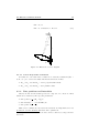
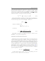
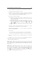
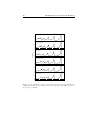
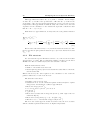
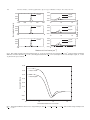
Upon launching the application, the GUI window is opened (see Fig. 1.1).
Figure 1.1: Graphical User Interface of the SPARTAN Code
The interface provides the following items which can be defined by the user:
1.1 Launching the SPARTAN code
5
1. Apparatus function: Here, the user can define a Gaussian apparatus
function of a given FWHM in Å for the simulation of experimentally measured spectra. this FWHM is added to the calculated Voigt FWHM.
Setting this option to 0 reproduces the “physical” spectra, for given local
conditions.
2. Rotational temperature: The user defines here the rotational temperature for the overall species1 . For the calculation of broadening mechanisms, the species translational temperature is considered to be equivalent
to the rotational temperature1 (Ttr =Trot ).
3. Vibrational temperature: The user defines here the vibrational temperature for the overall species1 .
4. Electronic excitation temperature: The user defines here the electronic excitation temperature for the overall species1 . Also, the free electrons temperature is considered to be equivalent to the electronic excitation temperature1 (Tel =Texc ).
5. Minimum wavelength: The user defines the minimum wavelength for
which the calculation is to be carried. If the maximum wavelength parameter is set to 0, this parameter is overridden and the overall spectra is
calculated.
6. Maximum wavelength: The user defines the maximum wavelength for
which the calculation is to be carried. If this parameter is set to 0, the
overall spectra is calculated.
7. Transitions database: The user selects the radiative transitions which
are to be calculated.
8. Calculate: Launches the calculation.
9. Total spectra: After the calculation is finished, this button reproduces
the overall spectra over the spectral range defined in boxes 5 and 6 (Minimum Wavelength and Maximum Wavelength). Setting a new minimum
and/or maximum wavelength and pressing the Total Spectra button will
reshape the graphical window to this new limits.
10. Single spectrum: After the calculation is finished, this button reproduces each radiative spectra with it’s associated color, over the spectral
range defined in boxes 5 and 6 (Minimum Wavelength and Maximum
Wavelength). Setting a new minimum and/or maximum wavelength and
pressing the Single Spectrum button will reshape the graphical window to
this new limits.
11. Erase: This button cleans the graphical window.
12. Record: This button records the overall spectra (IE_IA_nu_Total.txt),
and each radiative system spectra (IE_IA_nu_01..i.txt) in the OUTPUTS
directory. Each ASCII textfile contains columnwise values of the wavenumber, emission coefficient, and absorption coefficient.
1 The code can however consider different internal modes temperatures for each species, see
chapter 3.
6
Getting Started
13. X and Y axis scale: These two buttons allow the user to switch between
linear to logarithmic scales for both the X and Y axis.
Note that besides setting these parameters in the code GUI, the user must
define the local number density of the different species present in the simulated
gas. These values must be changed by the user in the Inputs.txt file in the
code INPUTS subdirectory.
1.1.2
How the Graphical User Interface works
The SPARTAN code GUI has been built as an upper layer to the core version of the SPARTAN code (SPARTAN_noGUI). The SPARTAN code receives it’s
calculation parameters from the file Inputs.txt (besides it’s other associated
files –Database.txt and Lineshape.txt– which will be further discussed in
chapter 3). The GUI commands merely updates the values of the Inputs.txt
file, without any interaction with the core of the SPARTAN code. Therefore,
this GUI can be straightforwardly overridden for coupled calculations using the
SPARTAN code and other numerical codes.
1.1.3
Other user-defined parameters
Besides the parameters modified through the GUI, and the local species
densities (in units of particle/m3 ) that have to be input in the file Inputs.txt,
many other parameters maybe adjusted by the user of the code. However these
imply a more detailed knowledge on the structure of the code and are discussed
in Chapter 3.
1.1.4
Running the SPARTAN code without the Graphical
User Interface
When using the SPARTAN code without using the program GUI, the
user must manually set the input parameters in the Inputs.txt file, record
the changes, and launch the calculation in the MATLAB command line by
typing >> SPARTAN_noGUI. Upon the calculation end, the code records the
overall spectra (IE_IA_nu_Total.txt), and each radiative system spectra
(IE_IA_nu_01..i.txt) in the OUTPUTS directory.
1.2
Recorded data
Each ASCII textfile for the the overall spectra (IE_IA_nu_Total.txt), and
each radiative system spectra (IE_IA_nu_01..i.txt) contains columnwise values of the emission coefficient (in W/m3 -cm−1 -sr), absorption coefficient (in
m−1 ), and wavenumber (in cm−1 ). Also, the code displays some of the calculation overall results, like the spectrum total radiative power, the radiative power
of each radiative transition, and the overall calculation time. Such parameters
are also recorded in the file Calc\_Log.txt, located in the OUTPUTS directory,
overriding any older logfile encountered in this directory.
Note that both versions of the code also leave the calculation parameters
(variables Inputs, Reference, Species, and Transitions) and results (vari-
1.3 Sample comparisons
7
ables Result for each radiative transition spectra, and ResultTotal for the
overall radiative spectra) in the MATLAB workspace.
1.3
Sample comparisons
A few supplied test routines showcase the capabilities of the SPARTAN
code for reproducing experimental spectra, and performing large scale spectral
computations.
Inside the TESTS directory there are several directories with a matlab executable each. These contain:
• A Simulation of the C2 ∆v = 0 Swan Bands, using the routine for the simulation of 3 Π −3 Π transitions for homonuclear molecules, and comparison
with an experimental spectrum.
• A Simulation of the CN Violet ∆v = 0 System, using the routine for
the simulation of 1 Σ −1 Σ transitions for heteronuclear molecules, and
comparison with an experimental spectrum.
• A Simulation of the H2 Lyman & Werner bands, using the routine for the
simulation of 1 Σ −1 Σ and 1 Π −1 Σ transitions for homonuclear molecules,
and comparison with an experimental spectrum.
• A Simulation of the N2 1st Negative ∆v = 0 System, using the routine
for the simulation of 2 Σ −2 Σ transitions for homonuclear molecules, including the effects of rotational perturbations, and comparison with an
experimental spectrum.
• A Simulation of the NO Rovibrational ∆v = 0 Transitions, using the routine for the simulation of 2 Π −1 Π transitions for heteronuclear molecules,
and comparison with an experimental spectrum.
• A Simulation of a full VUV–IR spectrum for Air at 1 bar mixture in full
thermochemical equilibrium at 1,000K and 6,000K.
• A Simulation of a full VUV–IR spectrum for a 97% CO2 –3% N2 1 bar mixture in full thermochemical equilibrium at 1,000K, 5,000K, and 10,000K.
An excel file (CO2N2_RadPower.xls) is also included, providing the integrated radiative intensity of a 97% CO2 –3% N2 mixture at 1bar and 4,300Pa.
1.4
Stepping a little further
This chapter has dealt with the essentials for a quick launch of the line-by-line
code SPARTAN, using its graphical interface. For the more detailed description
of the physical models implemented in the code, please refer to Chapter 2. For a
detailed description of the SPARTAN code structure and routines, please refer
to Chapter 3. For the information on how to customize the code for your specific
needs, please refer to Chapter 4.
8
Getting Started
Chapter 2
Physical Models
HΨ = EΨ
Schrödinger’s Equation
This Chapter provides an abridged description of the theoretical and numerical quantum models that have been implemented in the SPARTAN code.
The Chapter is split into three sections, which respectively describe the implemented theoretical models for the calculation of discrete radiation, the calculation of continuum radiation, and the generalized relationships between emission/absorption coefficients.
2.1
Discrete radiation models
The theory of discrete atomic and diatomic transitions is shortly summarized
in this section, starting with the selection rules, which indicate which radiative
transitions are allowed between the species different internal levels, followed
by the description of the models utilized for the calculation of line positions,
intensities, and shapes.
2.1.1
Selection rules
2.1.1.1
Atomic transitions
Atomic transitions are split into electric/magnetic dipolar or quadrupolar
transitions. The transitions can be classified by order of decreasing intensity: dipolar electric E1, quadrupolar electric E2, dipolar magnetic M1, and
quadrupolar magnetic M2. E1 transitions are called “allowed transitions”, the
others “forbidden transitions”. The selection rules [2] are summarized in Table
2.1
2.1.1.2
Diatomic transitions
Only electric dipolar transitions are considered for the calculation of synthetic discrete spectra from diatomic species, as the other type of transitions
have much lower probabilities and are generally covered by this stronger spectra.
10
Physical Models
Transitions E1
Transitions M1
Transitions E2
All couplings
1
∆J = 0, ±1
(except 0 = 0)
∆J = 0, ±1
(except 0 = 0)
∆J = 0, ±1, ±2
(except 0 = 0,
1
1
2 = 2 ,1 = 1)
2
∆M = 0, ±1
(except 0 = 0
when J = 0)
∆M = 0, ±1
(except 0 = 0)
when J = 0)
∆M = 0, ±1, ±2
3
parity change
identical parity
identical parity
one electron transition
with ∆l = ±1,
for arbitrary ∆n
no electronic
configuration
change, i.e.
for all electrons:
∆l = 0, ∆n = 0
no electronic
configuration
change, i.e.
for one electron:
∆l = 0, ±2,
∆n arbitrary
1
4
L–S Coupling
5
∆S = 0
∆S = 0
∆S = 0
6
∆L = 0, ±1
(except 0 = 0)
∆L = 0, ∆J = ±1
∆L = 0, ±1, ±2
(except 0 = 0,
0 = 1)
Table 2.1: Selection rules for atomic transitions
2.1 Discrete radiation models
11
The overall rotational lines of for the transitions between upper (e0 , v 0 , J 0 )
and lower (e00 , v 00 , J 00 ) levels which share the same ∆N and ∆J are written as:
∆N
∆Ji,j
where i and j stand for the index of the upper and lower states multiplet
components. Since for an electric dipolar transition we have i = j, the branches
with ∆J = ∆N are called “main branches”, whereas the branches with ∆J 6=
∆N are called “satellite branches”. The nomenclature for the different branches
is summarized in Table 2.2
∆J
∆N
N
O
P
Q
R
S
T
-3
-2
-1
-1
0
0
1
1
2
3
Table 2.2: Nomenclature for the different rotational branches
For diatomic transitions, three levels of coupling rules have to be accounted
for:
1. General selection rules
2. Selection rules for molecular angular momentum coupling Hünd Case a
3. Selection rules for molecular angular momentum coupling Hünd Case b2
We define the notations e and f which allow identifying a level parity. For
a integer rotational quantum number J we note e as the parity level (−1)J and
f the parity level −(−1)J . For a half-integer rotational quantum number J we
1
1
note e as the parity level (−1)J− 2 and f the parity level −(−1)J− 2 .
The general selection rules for diatomic dipolar transitions have been summarized by Herzberg [3], and are reported in table 2.3.
For the a et b Hünd cases, both Λ and S quantum numbers are defined, and
the following selection rules are observed:
∆Λ = 0, ±1
∆S = 0
(2.1)
additionally, for a Σ ↔ Σ transition we have
Σ+ ↔ Σ+ , Σ− ↔ Σ− allowed
Σ+ ↔ Σ− forbidden
(2.2)
For the a Hünd case, the quantum number Σ (not to be confused with the
electronic state Σ such that Λ = 0) is also defined. If both initial and final
states of the transition belong to Hünd case a, we have the selection rule
2 Other
very specific coupling cases also exist but are not considered in the code
12
Physical Models
transition between
rotational levels
∆J = 0, ±1
(except 0 = 0)
parity of the
rotational levels
+ ↔ − allowed
+ = +, − = − forbidden
e ↔ f allowed
e ↔ e, f ↔ f forbidden
rotational branches
Q(∆J = 0)
e ↔ e, f ↔ f allowed
e = f forbidden
rotational branches
P, R(∆J = ±1)
homonuclear molecules
s ↔ s, a ↔ a allowed
s = a forbidden
same charge cores
g ↔ u allowed
g ↔ g, u ↔ u forbidden
Table 2.3: Selection rules for diatomic electric dipolar transitions
∆Σ = 0
(2.3)
accounting for selection rules (2.1) and (2.2) we obtain the selection rule:
∆Ω = 0, ±1
∆J = 0 forbidden for Ω = 0 ↔ Ω = 0
(2.4)
6
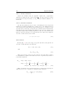
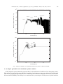
J
N
..........
........... ..................................
............
.....
...........
...
..........
....
......... ....
.........
....
.....
.............................
.......
.......
.......
.......
.......
........
.....
........
....
.........
....
.........
....
.......
.......... Λ Ω
Σ
........... }|
z
{........
r r .......................................
...........................
SR
L
R
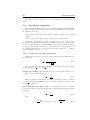
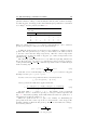
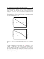
Figure 2.1: Hünd case a vector diagram
For the b Hünd case, the quantum number Σ is no longer defined. If both
initial and final states of the transition both belong to Hünd case b, we have the
selection rule
2.1 Discrete radiation models
13
∆N = 0, ±1
∆N = 0 forbidden for Σ ↔ Σ
(2.5)
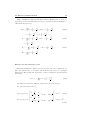
BM S
B
6
J K
N
r H
r Λ HH
H
j
L H
......................................
.
..........
..................................
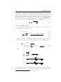
Figure 2.2: Hünd case b vector diagram
2.1.1.3
Linear Polyatomic transitions
In addition to the same rules considered for diatomic transitions (∆J =
0, ±1, etc..) we observe the additional vibrational selection rules:
1. ∆v2 + ∆v3 odd and ∆`2 = ±1 for perpendicular bands;
2. ∆v2 + ∆v3 odd and ∆`2 = 0 for parallel bands.
2.1.2
Line positions and intensities
Discrete atomic and molecular spectra are composed of a collection of lines
which can be defined by three specific parameters:
1. Line position: ν = (Eu − El )/h
2. Line intensity3 : ε = Nu Aul ∆Eul /4π
3. Line profile: F (ν − ν 0 )
This section outlines the theoretical models that are implemented for the
production of a line database with these three parameters.
3 absorption coefficients are determined from the emission coefficients according to Kirchoff–
Planck Law
14
Physical Models
2.1.2.1
Atomic transitions
Atomic line transition lists are typically compiled into comprehensive
databases providing the line center positions ν 0 , the upper and lower energy
level energies and degeneracies Eu , gu , El , gl , and the transition Einstein coefficients Aul .
2.1.2.2
Diatomic transitions
For diatomic transitions, the procedure of calculating the level energies and
transition probabilities is slightly more complex, due to the additional degrees
of freedom from molecular vibrational and rotational motion. As such, for each
electronic state of a molecule corresponds a set of vibration and rotational levels.
Following the Born–Oppenheimer approximation, the electronic, vibration and
rotational energies may be usually separated so that the total internal wave
function of the molecule may be decoupled in three wave functions grouping the
electronic, vibration and rotation terms:
ψ = ψel × ψvib × ψrot
(2.6)
Line Positions
Following Eq. 2.6, the total energy of a specific diatomic level is split into an
electronic, vibrational and rotational term:
Ee,v,J = Eel + Evib + Erot
(2.7)
Eel Evib Erot
(2.8)
with
These level energies correspond to the solutions of the Schrödinger equation
for an anharmonic oscillator and a distorted rotator, represented by a series of
polynomial expansions:
Ee,v,J = T (e) + G(v) + Fv (J)
2
3
1
1
1
− ωe x e v +
+ ωe ye v +
+ ···
= T (e) + ωe v +
2
2
2
+ Bv (J(J + 1)) − Dv (J(J + 1))2 + Hv (J(J + 1))3 + · · ·
(2.9)
These expressions can be presented in a more compact form replacing the
different spectroscopic constants by a Dunham matrix such that:
Ee,v,J =
X
i,j
i
Yij (v + 1/2) [F (J)]j ,
(2.10)
2.1 Discrete radiation models
15
This formalism is consistent with Zare’s effective Hamiltonian [4]. The correspondence between traditional spectroscopic expressions and the Dunham coefficients is then given by:
i
1
1
= T (e) + ωe v +
G(v) =
Yi0 v +
2
2
i=0, ...
2
3
1
1
+ ωe ye v +
+ ...
− ωe xe v +
2
2
i
X
1
1
Bv =
Yi1 v +
= Be − αe v +
2
2
i=0, ...
2
1
+ ...
+ γe v +
2
i
X
1
1
+ ...
= De + βe v +
Dv = −
Yi2 v +
2
2
i=0, ...
i
X
1
Hv =
Yi3 v +
,...
2
i=0, ...
X
(2.11a)
(2.11b)
(2.11c)
...
Energies for fine-structure levels
When spin-splitting is considered, we need to introduce the constants Av for
spin-orbit interactions, γv for spin-rotation interactions, and λv for spin-spin
interactions. The vibrational dependence of these constants is expressed in the
usual way:
i
i
X
1
[A, λ, γ]v =
[A, λ, γ]i v +
2
0
(2.12)
We will now present the different equations for the level energies.
For general doublet states [5]:
2
J + 12 − Λ2
21
F3/2 (J ≥ 1) = Bv 1 2
− 2 4 J + 12 + Yv (Yv − 4)Λ2
2
J + 12 − Λ2
21
F1/2 (J ≥ 0) = Bv 1 2
+ 2 4 J + 12 + Yv (Yv − 4)Λ2
− Dv J 4
(2.13a)
− Dv (J + 1)4
(2.13b)
16
Physical Models
For 2 Σ states [3]:
J
2
J +1
2
Σ1/2 (J ≥ 0) = Bv (J(J + 1)) − Dv (J(J + 1))2 − γv
2
2
Σ3/2 (J ≥ 1) = Bv (J(J + 1)) − Dv (J(J + 1))2 + γv
(2.14a)
(2.14b)
For 3 Σ states the energy levels expression is given by [6] from the formulation
of [7] with a typographic correction from [8]. This expression is deemed more
accurate than the general expression from [3]. The expressions read:
3
3
3
Σ2 (J ≥ 2) = Bv (J(J + 1)) − Dv (J(J + 1))2 − λv − Bv + 21 γv
h
2
2 i 12
− λv − Bv + 12 γv + 4J(J + 1) Bv − 12 γv
Σ1 (J ≥ 1) = Bv (J(J + 1)) − Dv (J(J + 1))2
2
1
2 γv
Σ0 (J ≥ 0) = Bv (J(J + 1)) − Dv (J(J + 1)) − λv − Bv +
h
2
2 i 12
+ λv − Bv + 12 γv + 4J(J + 1) Bv − 12 γv
(2.15a)
(2.15b)
(2.15c)
The expression for the 3 Π levels is given by [9]:
"
#
p
J(J + 1) − y1 + 4J(J + 1)
Π2 (J ≥ 2) = Bv
−
D
v J
− 32 yy21 −2J(J+1)
+4J(J+1)
4 y2 − 2J(J + 1)
3
− Dv J +
Π1 (J ≥ 1) = Bv J(J + 1) +
3 y1 + 4J(J + 1)
"
#
p
J(J + 1) + y1 + 4J(J + 1)
3
Π0 (J ≥ 0) = Bv
−
D
v J
− 32 yy21 −2J(J+1)
+4J(J+1)
3
4
1
2
4
−
(2.16a)
1
2
(2.16b)
+
3
2
4
(2.16c)
with
y1 = Yv (Yv − 4) +
4
3
y2 = Yv (Yv − 1) −
4
9
Yv =
Av
Bv
These expressions are also consistent with Zare’s effective Hamiltonian [4],
and one should be careful enough to select spectroscopic constants that have
been fitted to such formalism. If spectroscopic constants fitted to other formalisms are selected, they should be converted to Zare’s effective Hamiltonian
prior to insertion in the code. Table 2.4, reported from Ref. [10] presents the
correspondence between spectroscopic constants fitted to Zare’s Hamiltonian
and Brown’s Hamiltonian [11], which is also popular among spectroscopists.
Line Intensities
The intensity of one line will depend on the energy of the transition, the
population of the excited level, and the transition probability, described by its
2.1 Discrete radiation models
17
Brown
Zare
A
B
D
H
γ
p
q
Dp
Dq
Hp
Hq
A
AZ − 1/8 B
Z p
Z
B + 1/2q
D
H
γ Z − 1/2p
p
q
Dp+2q − 2Dq
Dq
Hp+2q − 2Hq
Hq
Z
Table 2.4: Spectroscopic constants correspondence for Brown’s and Zare’s
Hamiltonians
Einstein coefficient Aul . Here we will describe the method for the calculation of
such parameter.
Although we admit the separability of the electronic, vibrational and rotational modes of a molecule, according to the Born–Oppenheimer approximation,
electronic and vibrational configurations are intrinsically connected through the
different potential curves, and there is also a coupling between the molecular
rotational motion and the electronic cloud of the molecule due to the electrons
spin movement. The transition probability Aul can then be decomposed as a
product:
0 0
0
0
J
Aul = Aee00vv00 · AΛ
Λ00 J 00
0 0
The vibronic component Aee00vv00 can then be expressed as a function of the vi0 00
bronic transition moment Rev v using the following expression (in atomic units,
using wavenumber ν units over frequency ν units4 :
64π 4 ν 3 (2 − δ0,Λ0 +Λ00 ) v0 v00 2
Re
3hc3
(2 − δ0,Λ0 )
0 00 2
As the vibronic transition moment Rev v
cannot usually be resolved for
P v0 v00 2
Re
is
each multiplet transition, an average transition moment value
rather used. We then have:
0 0
Aee00vv00 =
0 00
Rev v
2
∼
=
P
0 00
Rev v
2
(2 − δ0,Λ0 +Λ00 )(2S + 1)
(2.17)
The vibronic transition moment is calculated using the electronic transition
moment Re (r) which is taken from the literature, and the upper and lower
4 The term 4π has an unit value in atomic units and hence does not appear explicitly in
0
the expression
18
Physical Models
states vibrational wavefunctions ψ which can be obtained by solving the radial
time-independent Schrödinger equation over recalculated potentials. This is
carried out by a companion routine of the SPARTAN code (RKR SCH) which
is described in appendix C. The relationship allowing to calculate the vibronic
transition moment for each upper/lower state pair reads as:
0 00
Rev v
2
=
Z
ψv0 (r)Re (r)ψv00 (r)dr
2
(2.18)
The rotational transition probability is in turn given by the different theoretical Hönl–London factors, which depend on the transition upper and lower
electronic states types (n Λ ↔n Λ) and the Hünd coupling case:
0
0
J
AΛ
Λ00 J 00 =
0
0
SΛΛ00JJ 00
2J 0 + 1
Using the normalization rule:
X
0
0
SΛΛ00JJ 00 (J 0 ) = (2J 0 + 1)
J 00
we then have:
Aul
P v0 v00 2
0 0
Re
64π 4 ν 3
SΛΛ00JJ 00
=
3hc3 (2 − δ0,Λ0 )(2S + 1) 2J 0 + 1
(2.19)
The analytic expressions for the Hönl–London factors considered in the
SPARTAN code are presented in appendix B.
Modeling of perturbations in the spectra
Perturbations in the spectrum can either affect the electronic states rotationless potential curves (avoided crossings), or affect the potential curves at
a given rotational quantum number (also avoided crossings). In the first case,
the vibrational-specific constants are modified after a given threshold vibrational
number, but this can be easily accounted for by using vibrationally-specific spectroscopic constants (Bv , Dv , etc...). For the case of rotational perturbations,
one can either resort to a complex approach of solving the perturbed system
Hamiltonian to yield the perturbed energy levels (see for example ref. [12]), or
the perturbation can be simply approached by an expression of the type 1/x
(see [3] pp. 283). In the SPARTAN code we have chosen this more simplified
approach, applying the equation:
EJ = EJ +
∆Emax
2 (J − Jpert − 1/2)
(2.20)
and using supplied values for ∆Emax and Jpert . The splitting of the exact
perturbed level in two different sub-levels is neglected.
2.1 Discrete radiation models
2.1.2.3
19
Linear Polyatomic transitions
The procedure for the calculation of linear polyatomic transitions (inserted
in the SPARTAN code due to the importance of CO2 IR radiation), is quite
similar to the one for diatomic transitions.
The emission coefficient is obtained as:
0
0
1
Nv0 J 0 Av0 v00 S``00 JJ00 FJ 0 J 00 hν
(2.21)
4π
where the additional term FJ 0 J 00 stands for the Hermann–Wallis factors,
which describe the interactions between the vibrational and rotational modes.
(see [3], p. 110).
εν =
The Einstein coefficient Av0 v00 for a purely vibrational transition is expressed
2
as a function of the square of the vibrational transition moment (Rv0 v00 ) according to the relationship
64π 4 3 (2 − δ0,`0 )
2
ν 0 00
(Rv0 v00 )
3hc3 v v (2 − δ0,`00 )
(2 − δ0,`0 )
2
= 2.026 · 10−6 ν 3v0 v00
(Rv0 v00 )
(2 − δ0,`00 )
Av0 v00 =
(2.22)
2
Since the numerical evaluation of the parameter (Rv0 v00 ) is quite complex,
it is customary to instead present the integrated intensity Svo0 v00 for a specific
vibrational band, calculated at a reference temperature T0 (usually 296K) [13].
The value of the dipolar moment (in atomic units (ea0 )2 ) can then be determined
from this parameter according to the relationship [14, 15]:
2
(Rv0 v00 ) Ia =
3hc 43 Svo0 v00
(ea0 )2
Qov
10
3
8π
ν v0 v00 (2 − δ 00 ) exp − hcEv0
D2
0,`
kB T0
(2.23)
The Hönl–London factors for these kind of linear vibrational transitions are
given by Ref. [16] and are presented in table 2.5:
∆` = 0
P
Q
R
00
00
00
00
∆` 6= 0
(J −1−`00 ∆`)(J 00 −`00 ∆`)
(J +` )(J −` )
00
J
2J 00
(2J 00 +1)`002
(J 00 +1+`00 ∆`)(J 00 −`00 ∆`)(2J 00 +1)
J 00 (J 00 +1)
2J 00 (J 00 +1)
(J 00 +1+`00 )(J 00 +1−`00 )
(J 00 +2+`00 ∆`)(J 00 +1+`00 ∆`)
J 00 +1
2(J 00 +1)
00
Table 2.5: Hönl–London factors for parallel and perpendicular rovibrational
transitions of linear polyatomic molecules
Lastly, the Herman–Wallis factors can be expressed as a function of the
following polynomial expressions:
P branch: (1 − A1 J 00 + A2 J 002 − A3 J 003 )2
Q branch: (1 + AQ J 00 (J 00 + 1))2
R branch: (1 + A1 (J 00 + 1) + A2 (J 00 + 1)2 + A3 (J 00 + 1)3 )2
20
Physical Models
The values for each coefficient A1,2,3,Q being tabulated for each vibrational
band.
2.1.3
Broadening mechanisms
Broadening mechanisms lead to the broadening of the initial transition Dirac
to a line following a specific shape. Broadening mechanisms can be split into
two different categories:
• Broadening from atomic and molecular collisions, described by a Lorentz
shape
• Broadening from Doppler effects, described by a Doppler shape
“Universal” expressions are presented in this section. Some of these expressions are in general approximate, but should suffice for the level of detail needed
for the typical applications of the SPARTAN code, proving flexible enough for
allowing an automated calculation of each transition broadening widths. All
broadening width units are presented in wavenumber units [cm−1 ], with the
species densities in [cm−3 ].
2.1.3.1
Collisional broadening mechanisms
Collisional broadening processes are described through a Lorentzian line profile such that:
`(ν) =
1+4
1
ν−ν 0
∆ν L
(2.24)
2
The convolution of different
P Lorentz line profiles also yields a Lorentz line
profile such that (∆ν L )tot = (∆ν L )i .
Natural broadening: The linewidth depends on the radiative lifetime τ according to the following expression:
1
(2.25)
4πcτ
This broadening mechanism is generally very small, and has accordingly
been neglected in the SPARTAN code. For example, a radiative lifetime of 1 ns
yields ∆ν N = 0.005 cm−1 .
∆ν N =
Pure collisional broadening: This process stems from the rate of collisions
between the different particles in the gas. The equivalent width has the following
expression:
∆ν C =
2νcol
c
(2.26)
with
νcol
106 X
2
=
Ni Nj π (ri [m] + rj [m])
Ni j
r
8kB
µi,j
π
(2.27)
2.1 Discrete radiation models
21
Resonance broadening: This broadening mechanism is confined to the electric dipolar atomic and molecular lines (resonance lines). An expression adapted
from [17] is used. In its current version, the SPARTAN code assumes all its
database lines as electric dipolar and as such applies this broadening mechanism to all its database.
∆λR = 1.2893 · 10
⇔ ∆ν R = 1.2893 · 10
−45
−13
gu
gl
gu
gl
21
12
Aul λ2 λ3R Ng
Aul
1
Ng
ν 3R
(2.28)
Van der Waals broadening: This broadening process stems from collisions
with neutral particles who do not share a resonant transition with the radiating
particle. The simplified expression from [18] is preferred to the expression from
[19], which is more precise but more difficult to implement:
∆ν W = 20(1.6 · 10
−33
4
·3 )
2
5
3kB T
m
3
10
1
N
c
where m = Nρ is the mean species mass and N = Ne +
particle density.
(2.29)
P
i
Ni the total
Stark broadening: This broadening process stems from the interaction between the external electronic shells of the radiating species and the plasma
charged species. Both ions and electron can account for such a broadening process, but in practice it is the electrons who contribute the most, due to their
higher kinetic speeds. We can therefore on a first approximation express Stark
broadening as a function of electronic density and temperature. Theoretical
expressions for the calculation of Stark broadening are not available, except for
hydrogenoı̈d species [18]. Tabulated values providing the parameter ∆λS as a
function of ne and Te are used [19]:
Ne
(2.30)
1016
In its current version, the SPARTAN code totally neglects Stark broadening,
due to the difficulties of implementing this broadening process in an universal
fashion. Future versions of the code will likely be updated to allow for some
amount of accounting for this process.
∆λS = f (Te )
2.1.3.2
Doppler broadening
Doppler broadening profiles follow a Gaussian shape and are described by
the following expression:
"
2 #
ν − ν0
g(ν) = exp −4 ln 2
(2.31)
∆ν G
As for the Lorentzian collisional lineshapes, the P
same additivity rule applies
for Doppler Gaussian-type lineshapes: (∆ν G )tot = (∆ν 2G )i
22
Physical Models
Doppler broadening is a consequence of the thermalized motion of the radiating species. A molecule radiating at a frequency ν0 in its own reference
plane, and approaching at a velocity v from the observation plane will
have a
Doppler-type shift in the observation plane, such that ν = ν0 1 + vc . Assuming a Maxwellian velocity distribution function at a characteristic temperature
T we may obtain the corresponding Doppler broadening width:
∆ν = ν 0
2.1.3.3
r
8 log 2
kB T
mc2
(2.32)
Voigt line profile
A Voigt profile results from the convolution of a Lorentz and
Doppler/Gaussian profile such that:
v(x) = `(x) ⊗ g(x)
r
Z
2
∆νL ln 2 +∞ exp − (ξ − x)2 ln 2 /∆νG
=
dξ
∆νG
π 3 −∞
ξ 2 + ∆νL2
x = ν − ν0
(2.33)
(2.34)
(2.35)
This profile cannot be analytically calculated and an approximate expression
needs to be used. Here we select the expression proposed by Whiting [20]5 :
2
C2
···
v(ν) = C1 e−4 ln 2D +
1 + 4D2
2.25
∆ν L
10
+ 0.016C2 1 −
e−0.4D
−
∆ν L
10 + D2.25
(2.36)
with
ν − ν0
∆ν V
q
1
∆ν V =
∆ν L + ∆ν 2L + 4∆ν 2G
2
∆ν L
1 − ∆ν
V
C1 =
∆ν 2L
∆ν L
∆ν V 1.065 + 0.447 ∆ν
+
0.058
2
∆ν
V
V
D=
C2 =
∆ν L
∆ν V
∆ν 2
∆ν L
+ 0.058 ∆ν 2L
∆ν V 1.065 + 0.447 ∆ν
V
V
This expression has been critically assessed by Olivero [21] who estimated
a precision with an accuracy of about 1% minimum. Olivero then proposed a
5 with
4ln 2 replaced by 2.772 for numerical efficiency reasons.
2.2 Continuum radiation models
23
modification to the Voigt linewidth parameter, improving the accuracy down to
0.02%:
∆ν V =
1
2
1.0692∆ν L +
q
0.86639∆ν 2L + 4∆ν 2G
In the SPARTAN code, we retain this analytical expression over the exact
convolution expression from Eq. 2.35, as it is significantly more computationally
efficient, specially in view of the sheer number of lines that have to be calculated
for the production of detailed spectra over a broad range.
2.2
Continuum radiation models
Continuum transitions are transitions in which one or both of the upper/lower states do not have a discrete energy, meaning that the radiation
spectrum will not have a discrete structure.
Continuum radiation transitions include:
1. Photoionization/Radiative recombination reactions:
A(n)+ + hν ↔ A(n+1)+ + e−
AB(n)+ + hν ↔ AB(n+1)+ + e−
(2.37)
2. Photodetachment/Photoatachment reactions:
A− + hν ↔ A + e−
(2.38)
3. Photodissociation–Dissociative Photoionization/Radiative association reactions:
AB + hν ↔ AB∗ ↔ A+B
AB + hν ↔ AB∗ ↔ A+ + B + e−
(2.39)
4. Bremsstrahlung/Inverse Bremsstrahlung reactions:
−
A + e−
i ↔ A + ef + hν
−
AB + e−
i ↔ AB + ef + hν
(2.40)
For these reactions, which include the emission or absorption of a free electron, energy conservation allows writing (with ∆Ei the ionization energy of the
atomic or molecular state):
1
(2.41)
hν = ∆Ei + me v 2
2
which means that this kind of radiative transitions will have an energy/frequency threshold below which they will not be able to occur.
24
Physical Models
2.2.1
Transition intensities
The transition intensities are usually expressed through calculated or
measured absorption cross-sections. These allow an immediate calculation of
the absorption coefficient, taking into account the population for the absorbing
states, and the calculation of the emission coefficient through detailed balancing, using the Planck–Kirchhoff law.
For processes 1–3, the expression for the absorption coefficient can be written
as:
α(ν) =
"
X
i
#
Ni σi (ν)
hν
1 − exp −
kB Te
(2.42)
provided that level-dependent
σi (ν)
h
spectral
i absorption cross-sections are
available. Here the factor 1 − exp − kBhνTe
allows for the subtraction of
stimulated emission processes, yielding the net absorption coefficient.
In certain cases only values for the global absorption cross-sections, tabulated
at different tabulated temperatures T , are available. In this case, the global
absorption coefficient, for an interpolated temperature T is written as:
hν
α(ν)T = N σ(ν, T ) 1 − exp −
(2.43)
kB T
For free-free Bremsstrahlung transitions (process 4), the absorption crosssection is written as:
hν
α(ν) = Ne N σ(ν, Te ) 1 − exp −
(2.44)
kB Te
2.2.1.1
Gaunt factors
A quantum correction for the classical absorption cross-section is usually
proposed in the form of a so-called Gaunt factor g which will depend on the gas
temperature T and the transition frequency ν. These corrective factors stem
from the analysis of high density stellar plasmas. The Gaunt factor is usually
close to unity. The correction to the classical absorption coefficient is simply
expressed as:
α(ν)quantum = α(ν) · g(ν, Tel )
(2.45)
The current version of the SPARTAN code accounts only for Free-Free
Gaunt factors, keeping the bound-free Gaunt factor gbf to unity.
The free-free Gaunt factor gf f is obtained for Tel>1 eV(11604 K) according
to the formulas proposed by Stallcop and Billman [22], who have adjusted the
results from Karzas and Latter [23] in numerical form. For Tel<1 eV, Hummer
[24] suggests considering the values provided by Menzel and Pekeris [25], who
provide a good approximation of the Gaunt factor for the temperature range
Te =[150–15000K] and for the wavenumbers ν=[10–350000cm−1 ].
2.2 Continuum radiation models
2.2.2
25
Special cases
Special cases, in which some additional approximations or some analytical
expressions are considered, are discussed in this section.
2.2.2.1
Photodetachment
Photodetachment transitions are typically modeled with the assumption
that:
1. Only the ground state of the negative ion contributes for the overall absorption coefficient.
2. The negative ions ground state is in a Saha equilibrium with the neutral
species ground state.
The Saha equilibrium equation becomes in this case:
NAB − = 0
2πµkB Tel
h2
3/2
QAB − (T )
NAB
0
h
i Q Q (T )
el AB
exp −1.4388 EAB − − EAB
(2.46)
0
with Qel = 2 and QAB − (T ) = gAB −
0
0
Photodetachment absorption cross-sections are then calculated in the usual
fashion:
hν
α(ν)T = NAB − σ(ν) 1 − exp −
(2.47)
0
kB T
2.2.2.2
Bremsstrahlung
Some analytic expressions for the calculation of the Bremstrahlung emission/absorption cross-sections are available in the literature.
The classical emission coefficient for the Inverse Bremsstrahlung of atomic
ionized species is given by Kramers [26]:
12 α2
6
hc
ν Ne Ni [MKS]
kB Te
(2.48)
Cross-sections for the Inverse Bremsstrahlung of N and O are provided by
Mjolsness and Ruppel [27]:
8
εν [J/m3 s sr Hz] =
3
√
σ(ν, Te ) = 8π 2 2π
2π
3kB Te me
2π
h
hc
√ e
4π0
√ e
4π0
me c3
2 h
i2
√ e
4π0
a0
i2
exp
23
1 hc
1 + 2 kB Te ν 5
kB Te
a 0 σ0
3
(hcν)
(2.49)
26
Physical Models
with σ0 =0.71 · 10−6 for O and σ0 =0.80 · 10−6 for N.
Tabulated N2 and O2 Bremstrahlung cross-sections σ(ν, T ) are reported in
Ref. [28]
2.3
Generalized Kirchhoff–Planck Law for radiative transfer
The detailed balance principle states that in full thermodynamic equilibrium, direct and inverse reaction processes fully balance themselves. Since
physical/chemical elementary processes do not depend on the thermodynamic
state of the gas/plasma, one may put to use the detailed balance principle to
deduce the intensity of an inverse process considering the intensity of the direct process and the expressions for the thermodynamic equilibrium of a gas.
The Law relating the radiative emission/absorption coefficients is the so-called
Kirchhoff–Planck Law, which will be shortly summarized for all the discrete and
continuum processes described in this chapter.
2.3.1
Discrete transitions
For discrete transitions of the type A, AB(i) → A, AB(j) the general
Kirchhoff–Planck Law, valid for any arbitrary population distribution of the
species internal levels, yields (in frequency units):
2hν 3
εν
= 2
α(ν)
c
gu Nl
−1
gl Nu
−1
(2.50)
In thermodynamic equilibrium conditions (with Ni = gi exp(−Ei /kB T )),
this expression becomes
−1
εν
2hν 3
hν
= 2 exp
−1
α(ν)
c
kB T
(2.51)
If we use wavenumber units ν (cm−1 ), the term 2hν 3 /c2 in Eq. 2.50 is
replaced by 2hc2 ν 3 . For wavelength units λ (Å), the term 2hc2 /λ5 is used.
2.3.2
Photoionization transitions
For photoionization/photodetachment processes such that AB(n)+ + hν →
, the relationship for the bound-free σbf (ν) photoionization absorption
AB
cross-sections, and the free-bound σf b (ν) radiative recombination cross-sections
is given by the Milne relations [29, 30]:
(n+1)+
σbf (ν)
1 me ve c 2 gi ge
=
σf b (ν)
2
hν
gn
(2.52)
If the electrons are thermalised and follow a Maxwell distribution function,
Eq. 2.52 can be further simplified to:
2.3 Generalized Kirchhoff–Planck Law for radiative transfer
σbf (ν)
gi 8kB me c2 Te
=
σf b (ν)
gn πh2 ν 2
The emission coefficient can then be calculated in the usual way:
hν
εν = Ni Ne σf b (ν) 1 − exp −
kB Te
27
(2.53)
(2.54)
Further if we have an Saha ionization equilibrium in the plasma, we can instead use the general Planck–Kirchhoff law of Eq. 2.51 for relating the emission
and absorption coefficients, by simply replacing T by Te .
2.3.3
Photodissociation transitions
For photodissociation processes such that AB(i) + hν → A+B, the relationship for the bound-free σbf (ν) and the free-bound σf b (ν) cross-sections is given
(in wavenumber [cm−1 ] units) by [31]:
2
(hcν)
σbf (ν)
= 23
σf b (ν)
µc 2 kB T
(2.55)
if we assume that the overall species translation velocities are Maxwellian.
Here µ in the molecular species reduced mass, in kg units.
2.3.4
Bremsstrahlung transitions
−
For Bremsstrahlung transitions such that AB+e−
i ↔ AB+ef + hν, if we assume that the electrons are thermalized (i.e. follow a Maxwell-Boltzmann vdf),
we may define the emission/absorption coefficients detailed balance through the
Planck–Kirchoff expression, proposed for the conditions of thermal equilibrium,
replacing the term T by Te :
−1
εν
2hν 3
hν
= 2 exp
−1
α(ν)
c
kB Te
(2.56)
28
Physical Models
Chapter 3
Detailed Description of the
Code
This Chapter provides a more detailed description of the code routines and
their associated functions. A full summary of the SPARTAN code capabilities
will be firstly presented, followed by a brief description of each of the core routines. Finally an extensive discussion of the algorithm for the Lineshape routine
will be presented. Indeed, knowledge on the inner workings of this routine is
paramount for a good understanding of the inner works of the SPARTAN code,
as over 99% of the overall calculation times are spent inside this routine, which
convolutes the lines lists supplied by the Atomic1,2,3 routines into a synthetic
spectrum. For a partial listing of the spectral database of the SPARTAN code,
please refer to Appendix A.
3.1
Introduction
The SPARTAN code has been developed with a particular concern in
providing a flexible and scalable structure. Rather than trying to provide an
“authoritative” tool with its own monolithic database, it has been acknowledged
that different applications will need more or less focus on different aspects
of the physical models implemented in the code. We also feel that with the
constant improvement of the state-of-the art in spectroscopy and modeling
30
Detailed Description of the Code
of physical-chemical processes in gases an plasmas (which is still undergoing
major progress at the time of this last manual update; 2013), it is important
that the code structure allows place for major future upgrades. For example,
progress in state-to-state modeling is likely to supersede more restrictive
approximations such as considering that the different species internal modes
follow a Boltzmann distribution.
With this in mind, a modular structure for the SPARTAN code has been
retained. The code itself is split into an excitation and a radiative module.
The excitation module is tasked with simulating the population of the different
upper and lower levels of radiative transitions, handling the calculated values
to the radiative module which then obtains the spectral-dependent emission
and absorption coefficients through the numerical routines which implement
the appropriate quantum-mechanic models. The calculation parameters are
supplied by an input file which can be bypassed if the code is utilized in a
coupled fashion (for example coupled to an hydro/plasma code). As stated
before, a GUI layer, which is totally independent from the code itself, is also
proposed. Finally, a fully-parametric spectral database is stored in a specific
folder, with each transition having its own file1 .
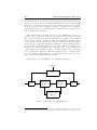
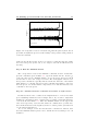
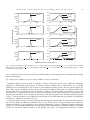
The structure of the SPARTAN code is summarized in Fig. 3.1.
Results
6
GUI
?
- Inputs
- Excitation
Module
- Radiative
Module
6
- Outputs
-
6
Spectroscopic
Database
Figure 3.1: Structure of the SPARTAN Code
1 With a small caveat in the sense that some continuum transitions, modeled by semiempirical expressions proposed by several authors, are hard-coded instead of being in a text
file
3.2 Summary of the capabilities of the SPARTAN code
3.2
Summary of the
SPARTAN code
capabilities
31
of
the
The SPARTAN code has been constructed with the aim of implementing
the most generalized physical models possible, trying to avoid the necessity of
resorting to any approximation of any kind, specifically when it comes to the
description of the thermodynamic state of the gas/plasma. A summary of the
physical models and capabilities of the SPARTAN code is summarized below:
• Simulation of discrete and continuum radiative transitions from
Atomic, Diatomic and Linear Triatomic molecules.
• Simulation of photoionization, photodissociation, photodetachment,
and Bremstrahlung transitions for atomic (when applicable) and diatomic species. Global or level-specific cross-sections can be considered.
• Voigt lineshapes for discrete spectra, including Doppler, collisional,
resonance, and van der Waals. Stark broadening is not considered at
this point (lack of a general expression).
• For discrete transitions from Diatomic molecules:
– Simulation of transitions between Σ, Π, and ∆ electronic states.
– Accounting for fine-structure transitions (singlet, doublet and
triplet), except for transitions involving ∆ electronic states which
only can be treated as singlet transitions.
– Accounting for Λ-doubling effects for homonuclear molecules.
– Transitions consider the intermediate a–b Hünd case for rotational
states.
– Level energies can be calculated either by using a Dunham matrix,
or with the input of vibrationally-specific spectroscopic constants.
– Simplified treatment of rotational perturbations.
• Individual Trot , Tvib , and Texc for each species. For now we assume
Ttr =Trot and Tel =Texc .
• Fully customizable database for the calculation of each species total
partition function. Vibrational partition function sum obtained either
from the truncated (at De ) harmonic oscillator approximation or from
the explicit
input of levels, Vibrational partition function sum obtained
P
from
QJ = Trot /(1.4388Bv )/σnuc , valid if Bv 1.4388Trot .
• Fully customizable spectral database.
• Variable spectral grid methods allowing the production of compact, yet
accurate synthetic lineshapes. A multitude of parameters, such as the
number of points of each Voigt lineshape, is user-parameterizable.
• De-coupled excitation and radiative modules, allowing for the direct
supply of nonequilibrium level populations by associated codes.
• General non-equilibrium Planck relationship between the emission and
absorption coefficients.
32
Detailed Description of the Code
3.3
Units used in the SPARTAN code
This is a short outline of the units for the critical variables used in the
SPARTAN code:
• Number density N (in Inputs.txt): m−3
• Wavenumber ν: cm−1
• Emission coefficient εν : W/m3 –cm−1 –sr
• Absorption coefficient α(ν): m−1
• Absorption cross-section σν : m3
3.4
Core routines
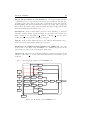
The core routines of the SPARTAN code are as follows:
Spectre.m is a general routine which cycles the code database, calculates the
individual spectra for the requested transitions, and superposes them to yield
the overall emission and absorption spectrum.
DataAtomic1,2,3.m routines read the database files for discrete atomic and
molecular transitions and handle the data to the corresponding Excite1,2,3.m
and Atomic1,2,3.m routines.
Excite1,2,3.m routines calculate the variables geE, NeE, NvE, geG, NeG, NvG,
considering a Boltzmann equilibrium of the internal states accounting for the
individual characteristic temperatures Texc , Tvib , Trot of the concerned chemical
species. These routines may be decoupled from the code, and general nonequilibrium populations for geE, NeE, NvE, geG, NeG, NvG may be injected by an
external function or file.
Atomic1,2,3.m routines build the spectral lines database for each calculated transition. They take as an input the spectral constants from the stored
database (handled by DataAtomic1,2,3.m inline functions of the Spectre.m
function), the general number densities of the different species of the cell
where spectral properties are being calculated (handled by Inputs.txt through
IORead.m and Spectre.m), and the upper/lower states populations and degeneracies (variables geE, NeE, NvE,geG, NeG, NvG), handled by the respective
Excite1,2,3.m functions. The routines then handle a 5 × n line matrix with
the 5 fundamental line parameters: line center ν 0 , emission coefficient εν , absorption coefficient α(ν), Doppler FWHM ∆ν G and Lorentz FWHM ∆ν G .
Raies1,2,3,1D,2D,3D are subfunctions of Atomic2.m which generate the line
lists for singlet or multiplet transitions.
3.4 Core routines
33
Photo1,2,T.m, PhoDet.m, and Bremstr.m are routines which calculate
continuum spectra for respectively monoatomic photoionization, diatomic photioinization/photodissociation, atomic photodetachement, and atomic/diatomic
Bremstrahlung, and yield an individual absorption spectrum. The corresponding emission spectrum is then generated inside the function Spectre.m using
the Planck/Kirchoff relationships of Sec. 2.3.
Lineshape.m is the routine which convolves a Voigt Lineshape to the Linedata lists of Diracs supplied by the Atomic1,2,3.m routines and yields a spectrum comprised of a wavenumber ν, emission coefficient εν , and absorption
coefficient α(ν), over a variable width spectral grid.
Glue.m is the routine which superposes the different individual spectra to
yield a global spectrum with a variable spectral grid.
GUInterface.m, GuiFunctions.m GUITrace.m, IOWrite.m Are functions specific to the GUI of the SPARTAN code. IOWrite.m updates the Inputs.txt file according to the user inputs from the GUI.
Integrate.m Integrates the individual radiative systems spectral dependent
emission coefficients εν to yield to their individual and the total radiative power
in W/m3 .
Fig. 3.2 presents the flowchart of the SPARTAN code.
Bremstr
PhoDet
Database.txt
Photo1
LoadDatabase
DataAtomic1
Excite1
Atomic1
Spectre
DataAtomic3
Excite3
Atomic3
IORead
DataAtomic2
Excite2
Atomic2
Convolve
Lineshape
Photo2
Inputs.txt
PhotoT
DATABASE
Figure 3.2: Flowchart of the SPARTAN code
Glue
RESULTS
34
Detailed Description of the Code
3.5
The Lineshape calculation routine
This lineshape calculation routine may be considered as the “core” of the
application. Indeed, even though setting up a line database may be a challenging task from a practical point of view2 , this poses no particular problem from
a numerical point of view. In fact, the problem can be solved efficiently using
vector programming, taking advantage of the capabilities of the MATLAB language. However, the convolution of a large number of lines with a Voigt profile
is a very intensive operation. Therefore, great care was exerted when developing
the line convolution routine, in order to achieve the shortest calculation times
alongside with a maximal precision of the calculated lineshapes. Furthermore,
the program routine has been built so as to allow the user to adjust a large array of parameters defining among others the number of points of the calculated
lineshapes. Still, the ratio of the time needed for the lines convolution and the
time needed for building up the line database is higher than 100 and increases
as the precision of the calculated lineshapes is increased.
In short, the user can define itself which is the level of precision required
in his calculations. More accurate lineshapes will require a large spectral grid
and larger computation times. Less precise calculations will allow defining preliminary calculations, or even allow affordable large-scale computations over a
fluid dynamics calculation grid. Some of the routine parameters can be easily
adjusted by users with a limited background on spectral lineshapes, others require a more extensive knowledge on the lineshape calculation methods and are
recommended to be kept at their default values.
The routine for the calculation of the computed spectra lineshapes, as well
as the overall user-defined parameters are described below. The user-defined
parameters can be adjusted editing the file Lineshape.txt in the INPUTS directory.
The Lineshape.m routine accepts as an input a matrix of size n×5 containing
the parameters for the calculation of n lines: wavenumber ν, emission coefficient
εν , absorption coefficient α(ν), Lorentz full width at half maximum (FWHM)
∆ν L , and Doppler full width at half maximum (FWHM) ∆ν G . The routine then
outputs the overall spectra wavenumber, emission and absorption coefficients.
The routine works as follows:
1. Separates the lines among three different categories: strong, weak, and
very weak (according to the parameters LinPar.[threshold1, threshold2])
2. Defines which lines are to be explicitly calculated, and which are to be
calculated as a “pseudo-continuum”. strong lines are calculated explicitly, very weak lines are calculated as a “pseudo-continuum”, weak lines
are calculated explicitly if they are not covered by a strong line. If the
“pseudo-continuum” is not selected (LinPar.contmethod=0) we have two
possibilities:
(a) The emission and absorption intensities of the explicitly calculated
lines are multiplied by a constant factor to account for the intensities
of the discarded lines and enforce energy conservation.
2 adequate spectroscopic constants for the calculation of line positions and intensities need
to be selected, along with the adequate expressions issued from spectroscopic theory.
3.5 The Lineshape calculation routine
35
(b) No further action is carried aside from discarding the weak lines.
In either cases steps 3 and 8 are overrided.
3. Intensities of the lines calculated as a “pseudo-continuum” are distributed
in slots over a fixed step wavelength (LinPar.ContStep) ranging from the
“pseudo-continuum” lines lower to higher wavenumber.
4. For each line calculated explicitly:
(a) Checks if the Doppler and Lorentz broadening widths of the current and former calculated line differ from more than a user-defined
parameter (LinPar.diff).
(b) YES: Calculates the line center distance and intensity for each of the
user-defined (LinPar.[ksi, beta, ksi1, beta1, num c, num w, par c,
par w, par w FG]) lineshape points, using a Voigt profile.
(c) NO: Uses the former calculated line gridpoints, sparing calculation
time.
5. Stores the overall points in ascending order (from lower to higher
wavenumbers) for the determination of the spectral grid.
6. Removes the points which are too close (according to the user-defined
parameter LinPar.minstep)
7. For each line:
(a) Selects the grid points which fall under the calculated lineshape.
(b) Interpolates and adds the line intensities to the new gridpoints region.
8. Interpolates and adds the “pseudo-continuum” intensities to the calculated
grid.
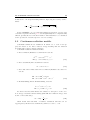
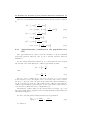
A schematic view of the selection process of the different lines, split into
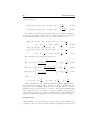
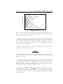
strong, weak, and very weak categories, is presented in Fig. 3.3
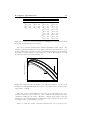
The user-defined parameters are:
LinPar.interp: This parameter defines the point’s interpolation method used
for the routine. The two possibilities are linear and cubic. linear interpolations are fastest but less accurate than cubic. It is recommender to use cubic
interpolations.
LinPar.shape: This parameter allows the user to allow the calculation of a
general Voigt lineshape (parameter 99), computed with a user-defined number of points for the lineshape core and the wings (LinPar.num c and LinPar.num w=6), or to allow the calculation of a simplified Voigt profile with 5,
7, 9 or 11 points (respectively parameters 5, 7, 9, or 11). For more details on
the calculation of the Voigt profile see section 3.5.1.
36
Detailed Description of the Code
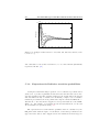
0
10
Strong
Weak
Very Weak
−1
10
−2
10
−3
Intensity (A. U.)
10
−4
10
−5
10
−6
10
−7
10
−8
10
−9
10
2.48
2.485
2.49
2.495
2.5
2.505
Wavelength (A)
2.51
2.515
2.52
4
x 10
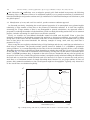
Figure 3.3: Example of Strong, Weak, and Very weak lines
LinPar.LineBound: Parameter which defines the boundary inside which a
high resolution lineshape is calculated and core and wings points are distributed
(see section 3.5.1 for more details). This parameter is dependent on parameter
LinPar.threshold1. 20 is recommended for LinPar.threshold1=1e3, higher values
are recommended for higher thresholds.
LinPar.ksi: Parameter which defines the Lorentz weight parameter defining
the boundary between the lineshape core and wings regions (see section 3.5.1
or [1] for more details). The recommended value for this parameter is 1.8.
LinPar.beta: Parameter which defines the Gauss weight parameter defining
the boundary between the lineshape core and wings regions (see section 3.5.1
or [1] for more details). The recommended value for this parameter is 1.
LinPar.ksi1: Parameter which defines the Lorentz weight parameter defining
the boundary between the lineshape wing and far wings regions. (see section
3.5.1 or [1] for more details). The recommended value for this parameter is 5.8.
LinPar.beta1: Parameter which defines the Gauss weight parameter defining
the boundary between the lineshape wing and far wings regions. (see section
3.5.1 or [1] for more details). The recommended value for this parameter is 5.8.
LinPar.num c: Number of points of the lineshape half core region (including
line maximum). Total number of points in the core region of the lineshape:
2 × LinP ar.num c − 1. Recommended values: from 3 to 6.
LinPar.num w: Number of points of the lineshape half wing region. Total
number of points in the wings region of the lineshape: 2 × LinP ar.num w.
Recommended values: from 6 to 12.
3.5 The Lineshape calculation routine
37
LinPar.par c: Parameter defining the core points distribution spacing (see
section 3.5.1 or [1] for more details).
LinPar.par w: Parameter defining the Lorentz contribution for wings points
distribution spacing (see section 3.5.1 or [1] for more details).
LinPar.par w FG: Parameter defining the Gauss contribution for wings
points distribution spacing (see section 3.5.1 or [1] for more details).
LinPar.diff: Maximum difference among the Gauss and Lorentz lineshapes of
two different lines for which the Voigt profile is not recalculated for the second
line. Recommended value: 0.1 corresponding to a 10% difference.
LinPar.Lorentz: LinP ar.Lorentz × F W HM is the minimum distance from
the line center where the line profile is considered to be Lorentzian. Recommended value: 64.
LinPar.cutoff: LinP ar.cutof f ×F W HM is the distance from the line center
where the line intensity is considered to be negligible (Intensity=0). Recommended value: 1000.
LinPar.minstep: Minimum interval between two adjacent lineshape points
(F W HM ×LinP ar.minstep). This parameter is useful for defining the accuracy
of the calculated line peaks. If the parameter is set to 99, it will be equivalent to
the minimum distance between adjacent points of the computed Voigt profile.
Recommended value: 99.
LinPar.intstep: Grid size for the calculation of the lineshape integral in the
core region. Recommended value: 120
LinPar.integral: Line normalization carried over the integral of a high resolution Voigt lineshape 1 or the integral of the selected lineshape for the overall
calculations. When computing a low resolution profile, setting this option to
0 will allow the line peaks will have the correct intensities, but the overall line
energy will not be accurate. Setting this option to 1 will yield less accurate
line peak intensities, but will allow the correct overall line energy. For higher
resolution lineshapes (LinP ar.shape = 99) it is recommended to keep the value
at 0.
LinPar.contmethod: Method used for accounting for the presence of weak
lines. Setting this option to 1 uses the “pseudo-continuum” method. Setting
this option to 0 discards the lines not calculated by the “Line-by-Line” method.
LinPar.addWeakLines: Setting this option to 1 homogeneously
hadds the discarded linesPintensitiesPto the icalculated lines intensities
strong
weak
weak
weak
/ Iemi,abs
Iemi,abs
= Iemi,abs
× 1 + Iemi,abs
.
Setting this option
to 0 simply discards the lines.
38
Detailed Description of the Code
LinPar.threshold1: Threshold (normalized to the maximum line emission
intensity OR the maximum line absorption intensity) above which a line is
selected to be calculated using the “Line-by-Line” method. Recommended
values: 103 − 106 Higher values will have more lines included in the overall calculation, yielding more accurate spectra, at the cost of larger memory
an computation time overheads. Note that for consistency, one must have
LinP ar.threshold1 ≤ LinP ar.threshold2
LinPar.threshold2: Threshold (normalized to the maximum line emission
intensity AND the maximum line absorption intensity) below which a line intensity contribution is added as a “pseudo-continuum” to the overall spectrum.
Recommended values: 104 − 107 Higher values will have less lines quickly calculated as a “pseudo-continuum, yielding more accurate spectra, at the cost of
larger memory and computation time overheads. Note that for consistency, one
must have LinP ar.threshold1 ≤ LinP ar.threshold2
LinPar.dnu: LinP ar.dnu × F W HMmed is the boundary (from the line center) defining the region were a weak line is covered by a strong line (making
it’s calculation as a “pseudo continuum” viable). Recommended value: 20 if
LinP ar.threshold2
3
LinP ar.threshold1 = 10 . For higher values of this ratio, it is recommended to
increase LinP ar.dnu.
LinPar.contstep: LinP ar.dnu × F W HMi is the fixed spectral width step of
the grid used for the calculation of the “pseudo-continuum” spectrum. Recommended value: 20.
3.5.1
Calculation of a Voigt lineshape
This subsection presents a more detailed description of the Voigt lineshape
calculations carried in step 4.b (see section 3.5).
The main objective is to ensure the calculation of a line profile as close
to Eq. 2.36 as possible, while retaining a minimum number of points. The
method implemented in the SPARTAN code yields profiles which are found
to adequately approximate the Voigt profile of Whiting & Olivero to a userdefined precision which will depend on the number of considered grid points.
The routine discriminates two sets of Voigt line profiles: a low resolution set
which allows quick spectral calculations yielding a compact overall spectral grid,
and a high resolution set for more smooth and detailed line profiles, at the cost
of larger spectral grids.
Four low-resolution Voigt line profiles with respectively 5, 7, 9 and 11 grid
points have been defined, introducing the parameters W and F W which define
the boundaries between the line center region, the “near” line wings, and the
“far” line wings respectively. The expression for those parameters, for a given
Voigt profile, is proposed by Zhu [32]:
2
(1 + ζ)∆ν L + β∆ν D
(3.1)
π
the [ζ, β] constants are held at [1,1.8] for the calculation of the parameter
W , as proposed by Smith [33], and held at [2.6,5.8] for the calculation of the
[W, F W ] =
3.5 The Lineshape calculation routine
39
parameter F W according to a critical analysis carried by Lino da Silva on sample
Lorentz, Doppler, and Voigt profiles. The different grid points have been defined
accordingly3 , and are presented in Table 3.1.
Number
of Points
Selected Points
ν0
5
7
9
11
×
×
×
×
V/8
×
V/2
W
FW
25V/2
×
×
×
×
×
×
×
×
×
×
×
×
×
Table 3.1: Gridpoints for 5, 7, 9, and 11 points lineshapes. An × defines a
specific point being accounted for in the given lineshape
A different method has been devised for the calculation of high resolution
profiles. Two line parameters parc and parw have firstly been defined, related
to the line center and line wings respectively. The line center being identical whether the profile is Lorentz or Doppler, parc will be independent of the
parameters ∆ν L and ∆ν D .
The lineshape wings will however be very different regarding whether the
line profile is Doppler or Lorentz. parw will therefore have a strong dependence
on the parameters ∆ν L and ∆ν D , and such dependence has been acknowledged
in the following way:
∆ν D
parwD
(3.2)
∆ν D + ∆ν L
such that for a Lorentz lineshape we have parw = parwL and for a Doppler
lineshape we have parw = parwL + parwD .
parw = parwL +
A series of monotonous points has then been defined such as
i0 = [0 : max/(numc − 1) : max]
and a geometrical transform is applied such that
1 − exp par(c,w) × i0 (1) / exp par(c,w) × i0 (max)
i=
1 − exp par(c,w) × i0 (1) / exp par(c,w) × i0 (max)
(3.3)
(3.4)
We then define ic = i and iw = 1 − i. An example of the geometrical
transforms ic and iw , obtained for specific parc and parw values, is presented in
Fig. 3.4. Practically speaking, such transformations return two grids more or
less tightened around the values 0 or 1.
These two grids need now to be put to use. Firstly, for distributing the
grid points in the line center region, the second derivative of the Voigt profile
is firstly calculated. Then the line profile points ν i are determined according to
the following relation:
ic =
3 Considering
v 00 (ν i )c
max[v 00 (ν i )c ]
a zero line intensity for the last grid point
(3.5)
40
Detailed Description of the Code
1
Normalized Transformation Value
0.9
0.8
parc=2.00
parc=1.00
parc=0.50
0.7
parc=0.25
0.6
0.5
parw=0.25
0.4
parw=0.50
0.3
0.2
0.1
0
0
parw=1.00
parw=2.00
0.2
0.4
0.6
Normalized Number of Points
0.8
1
Figure 3.4: Plot of the numerical transforms yielding the unevenly-spaced gridpoints ic and iw from the evenly-spaced gridpoints i, for different values of the
adjustable parameters parc and parw .
Which means that the spectral grid will be tighter in the profile regions with
large second derivatives (near the line center). Here, the second derivative is
a good variational parameter as it allows an optimum distribution of lineshape
points, ensuring an adequate reproduction of the exact lineshape through the
linear connection of such points.
The line wings structure is such that the optimal grid points distribution is
considered to be given by the relation
iw =
v(ν i )w
max[v(ν i )w ]
(3.6)
Which allows distributing the grid points efficiently in the “far” wings regions
where the intensity decrease is very slow (thus explaining the tightening of the
parameter iw near 0).
We may now assign a given number of points to be distributed near the line
center and the line wings. The calculation routine then proceeds according to
the described method in order to optimally distribute such points. More precise
line profiles will be obtained for a larger number of assigned grid points, at the
cost of increased spectral grids and calculation times.
Different low and high resolution lineshapes have been compared with the
exact Voigt profiles (Eq. 2.36) with ∆ν=5 cm−1 . The differences to the exact
profile have also been determined for each of such profiles. The obtained results
are presented in Fig. 5 for low resolution profiles, and in Fig. 6 for high
resolution profiles.
3.5 The Lineshape calculation routine
0.5
0.06
Lorentz
Doppler
0.1
−100
0
Normalized Intensity
0.06
100
200
Lorentz
2
10
Lorentz
Doppler
0.1
0.02
−100
0
0.06
100
200
Lorentz
−0.1
0
10
0.5
1
10
2
10
Lorentz
0.3
0.04
Doppler
0.1
0.02
−100
0
0.06
100
200
Lorentz
−0.1
0
10
0.5
1
10
2
10
Lorentz
0.3
0.04
Doppler
0.1
0.02
0
−200
1
10
0.3
0.04
0
−200
−0.1
0
10
0.5
Difference to Exact Intensity
0.02
0
−200
Lorentz
0.3
0.04
0
−200
41
−100
0
100
200
−0.1
0
10
1
−1
10
2
10
Distance to Line Center (cm )
Figure 3.5: Plot of low resolution Lorentz lineshapes (left; 5, 7, 9 and 11 points
from top to bottom; ∆ν=5 cm−1 ) and plot of the normalized difference of
Lorentz (full line; ∆ν=5 cm−1 ) and Doppler (dotted line; ∆ν=5 cm−1 ) lineshapes to the exact lineshapes (right; 5, 7, 9 and 11 points from top to bottom).
0.05
0.06
Lorentz
Normalized Intensity
−100
0
0.06
100
200
Lorentz
2
10
Lorentz
Doppler
0.01
0.02
−100
0
0.06
100
200
Lorentz
−0.01
0
10
0.05
1
10
2
10
Lorentz
0.03
0.04
Doppler
0.01
0.02
0
−200
1
10
0.03
0.04
0
−200
−0.01
0
10
0.05
Difference to Exact Intensity
Doppler
0.01
0.02
0
−200
Lorentz
0.03
0.04
−100
0
100
200
−0.01
0
10
1
−1
10
2
10
Distance to Line Center (cm )
Figure 3.6: Plot of high resolution Lorentz lineshapes (left; 21, 37, and 73
points from top to bottom; ∆ν=5 cm−1 ) and plot of the normalized difference
of Lorentz (full line; ∆ν=5 cm−1 ) and Doppler (dotted line; ∆ν=5 cm−1 ) lineshapes to the exact lineshapes (right; 21, 37, and 73 points from top to bottom).
42
3.5.2
Detailed Description of the Code
Handling and Overlay of Individual Lineshapes
Following the definition of a method for adaptively calculating individual
lineshapes, one may apply it to the calculation of the individual lineshapes for
each of the calculated radiative transitions (with their accompanying Doppler
and Lorentz FWHM). However doing so for a large number of lines (typically
more than 104 ) might still yield large calculation times. One can acknowledge that the systematic evaluation of exponential terms of Eq. 2.36 for the
calculation of several thousand lines might be an ineffective method. Instead,
one can take advantage of the fact that the different lineshapes Doppler and
Lorentz FWHM remain very close over a large spectral range. The calculated
lineshapes are then nearly equivalent and there is no need to systematically
recalculate them.
As an example, the differences between two Voigt lineshapes, for a 10%
variation of their Lorentz and Doppler FWHM, is presented in Fig. 3.7. Given
the small differences between such spectra, one may chose not to recalculate a
spectral lineshape if both the Lorentz and Doppler FWHM differ less than by
a given percentage (10% being an adequate value).
0.06
0.05
+10% Lorentz
Normalized Difference
0.04
+10% Doppler
0.03
0.02
0.01
0
−0.01
−0.02 −2
10
−1
0
10
10
Normalized Distance to Line Center
1
10
Figure 3.7: Normalized difference between two Voigt lineshapes with ∆ν 0L =
1.1∆ν L & ∆ν 0D = 1.1∆ν D , and an initial Voigt lineshape with ∆ν L,D = 5cm−1 .
Such approach further improves computational efficiency, as for most of the
transitions to be simulated, the calculation routine merely replicates the previous lineshape spectral grid points and relative intensities, simply multiplying the
relative line intensities by the line strength to yield the absolute line intensities.
Once that the spectral lineshapes have been calculated for each of the overall
database transitions, such individual lineshapes have then to be combined to
yield an overall spectra.
This is firstly done considering the overall calculated grid points and grouping them in an increasing order. Secondly, the spectral points too close to each
other by a defined parameter (named minstep and typically 1/40 of the FWHM)
are grouped. Finally, each individual lineshape is interpolated over the boundaries of the overall spectral grid which falls inside the first and last grid points
3.5 The Lineshape calculation routine
43
of the individual lineshape. The overall discrete spectrum is then overlaid to the
previously calculated “pseudo-continuum” spectrum to yield the final spectrum.
In brief, this proposed adaptive grid method represents an approach where a
series of approximations (“pseudo-continuum”, calculation of Voigt lineshapes
with a minimum number of points, non-systematic lineshape recalculation) are
carried in order to achieve consequent reduction of calculation times and spectral grids. One more advantage of the proposed method is the fact that it is
fully user-parameterizable, and allows one to chose the level of accuracy (with
the associated memory and computational overheads) when carrying spectral
calculations.
44
Detailed Description of the Code
Chapter 4
Modifying the Code
Spectral Database
.
“With Great Power comes Great
Responsibility”
Voltaire
4.1
Introduction
This Chapter provides an in-depth description of the spectral database
structure of the SPARTAN code, with the description of the necessary steps
for its update or upgrade, according to the user needs.
The capabilities of the SPARTAN code are summarized in Table 4.1. BoundBound transitions are all treated through its own subroutines (AtomicX.m),
which implement the theoretical models described in Chapter 3. Bound-Free
transitions are subdivided in photoionization, photodissociation (for diatomic
and triatomic molecules) and photodetachment transitions, which can either
use total or state-specific cross-sections. Finally Free–Free transitions are hardcoded in their own routine (Bremstr.m).
Discrete transitions from diatomic species play a predominant part in the
spectral features of gases and plasmas. As such, the databases for the simulation
of these transitions are the most liable to be the subject of extensions and
updates. Accordingly, we will begin this section by providing some guidelines for
the selection of an appropriate spectral database for any given bound diatomic
transition. We will then follow with the description of the steps necessary for the
construction of the datafiles for the calculation of bound diatomic spectra. Next
we will describe how to update the databases for the other transitions (bound
transitions for atomic and linear triatomic species, and continuum transitions,
including a description of the hard-coded Free–Free transitions). Finally we
will close this tutorial Chapter through the description on how to link any new
spectral databases to the SPARTAN code.
46
Modifying the Code Spectral Database
Atomic
Diatomic
Triatomic
Linear
User-defined User-defined User-defined
(Atomic1.m) (Atomic2.m) (Atomic3.m)
Bound–Bound
Total
–
Photoionization
User-defined
(PhotoT.m)
Level User-defined User-defined
Specific (Photo1.m) (Photo2.m)
Bound–Free
Total
–
User-defined
(PhotoT.m)
Level
Specific
–
User-defined
(Photo2.m)
–
User-defined
(PhoDet.m)
Photodissociation
Photodetachment Total
Free–Free
(Bremstrahlung)
Hard-coded Hard-coded
(Bremstr.m) (Bremstr.m)
–
–
Table 4.1: Transitions modeled by the SPARTAN code, corresponding numerical
routines, and spectral datafile types
4.2
Building spectral datafiles for diatomic transitions
This section provides an in-depth description on how to create and modify
spectroscopic constant files in a format compatible with the SPARTAN code,
and provides some guidelines for the appropriate selection of spectral data which
is consistent with the user needs.
4.2.1
Guidelines for the selection of appropriated spectral
constants
When deciding to develop a new spectral database for a specific diatomic
transition, one first needs to examine the degree of accuracy of the spectral
constants that can be found in the literature. It is then necesary to inquire
up to which degree the spectra might be affected by perturbations by another
states.
As discussed briefly in Chapter 2, three levels of detail can be considered
when creating/modifying the spectral database for a specific diatomic transition:
1. Selection of a Dunham matrix providing the expressions for the rovibronic
energies for any arbitrary values of v and J, according to the expressions
of Eq. 2.10.
2. Selection of a set of vibrationally-specific constants Bv , Dv , . . . for a given
set of vibrational levels vi , allowing the calculation of the level energies
for any arbitrary rotational quantum level J (see Eqs. 2.11).
4.2 Building spectral datafiles for diatomic transitions
47
3. Selection of the energy shifts around a specific rotational quantum number
Ji , for a given vibrational quantum number vi . This treatment is necessary
for the accounting for rotational perturbation effects and is carried in
addition to considering either a set of equilibrium or vibrationally-specific
spectroscopic constants.
Usually, selecting an appropriate Dunham matrix with up-to-date spectroscopic constants is sufficient for most general radiative transfer applications. For
the accurate reproduction of measured spectra (with FWHM<1Å) it is sometimes necessary to supply level-specific spectroscopic constants to complement
the equilibrium constants.
Another aspect to take into consideration is the order of the spectroscopic
constants that are selected. Due to the inherent oscillatory characteristics of
polynomial expansions such as those depending on v + 1/2 for vibrational levels, and J(J + 1) for rotational levels, a dataset with larger order corrective
spectroscopic constants will be able to reproduce a broader range of vibrational/rotational quantum numbers v/J, but a dataset with lower order corrections will usually provide better extrapolations beyond the initial fit validity
range. Therefore, as a rule of thumb, the higher the order of the spectral constants corrections (in polynomial form), the most likely that the level energies
above the range of the fitted v and J numbers will strongly diverge from their
exact values.
The selection of an appropriate Dunham matrix can by itself allow the calculation of a synthetic spectrum which accurately reproduces experimental results.
Spectroscopy techniques have known almost spectacular developments over the
last 50 decades, and increasingly accurate data, valid for a broad range of vibrational and rotational levels, has been made available in the most recently
years, usually as the result of the application of very detailed Fourier transform
spectroscopy methods. A striking example for such developments can be provided for the CN Violet ∆v = 0 spectrum, who is ubiquitous in most of air
and carbon chemistry plasmas. This system has a very clear bandhead structure which can be detected up to v = 8 − 9, with a band reversal from the
ultraviolet direction towards the infrared direction starting at v = 4 − 5, whose
bandheads are experimentally overlapped. In Fig. 4.1, an experimental spectrum issued from an arcjet low-pressure wind-tunnel [1] is compared against
several synthetic spectra produced using the best-fit vibrational and rotational
temperatures Tvib = 10800 ± 100 K and Trot = 4900 ± 100 K, and applying several
sets of Dunham coefficients.
One may verify that the reproduction of the higher vibrational number bands
is increasingly poorer when resorting to older spectral datasets. Namely, the
v = 4 − 5 bandheads can only be accurately reproduced with the most recent
datasets issued from Fourier transform spectroscopy techniques1 .
In some specific cases, equilibrium constants will not provide sufficient accuracy for the reproduction of experimental spectra. Sometimes, this might
be related to the extra loss of precision resulting from the extra fit from level1 However, even such techniques may sometimes not be adapted for the reproduction of
high-temperature spectra in such cases where lower temperatures of the gas/plasma are imposed so as to have very little Doppler broadening of the measured lines, which comes at a
cost of a lower Jmax of the fit, since higher rotational levels will not be sufficiently populated
at such values for T .
48
Modifying the Code Spectral Database
1
Herzberg 1965
0.5
0
1
Huber & Herzberg 1979
.
0.5
0
1
Intensity (A.U)
NEQAIR 1985
0.5
0
1
Cernyi 1978 & Ito 1988
0.5
0
1
Prasad & Bernath 1992
0.5
0
1
Measured Spectrum
0.5
0
3840
3850
3860
3870
Wavelength (A)
3880
3890
Figure 4.1: Comparison between a CN Violet ∆v=0 spectrum measured in
a high-temperature arcjet facility and several spectra using different sets of
spectroscpic constants
4.2 Building spectral datafiles for diatomic transitions
49
1.64
0.01
1.62
0.008
0.006
1.6
0.004
1.58
0.002
1.56
0
1.54
−0.002
1.52
Fit Dispersion (cm−1)
Bv(a3Πu) Rotational Constant (cm−1)
dependent spectroscopic constants to the more “universal” Dunham spectroscopic coefficients. More often, this is the result of vibrational perturbations
in the upper or lower levels of the spectra, which are the results from “avoided
crossings” of these states rotationless potentials. In this case, the shape of the
potential curve will change dramatically after a critical vibrational number v,
and the level spectroscopic constants will see a sharp change in their trends, disallowing their proper reproduction through the use of polynomial expressions
depending on the variable (v + 1/2).
−0.004
1.5
−0.006
1.48
1.46
0
−0.008
1
2
3
4
5
6
7
8
−0.01
9
Vibrational Quantum Number
1.8
0.01
0.008
0.006
1.7
0.004
1.65
0.002
1.6
0
−0.002
1.55
Fit Dispersion (cm−1)
Bv(d3Πg) Rotational Constant (cm−1)
1.75
−0.004
1.5
−0.006
1.45
1.4
0
−0.008
1
2
3
4
5
6
7
8
9
−0.01
10
Vibrational Quantum Number
Figure 4.2: Interpolation of the level-specific rotational constants Bv for the
unperturbed a3 Πu (top) and the perturbed d3 Πg (bottom) electronic states of
C2
One example can be presented for the C2 Swan bands system, who is also
generally ubiquitous in carbon-based plasmas. Fig. 4.2 shows the fit of the
constants Bv for unperturbed lower a state, and for the perturbed d state.
One may immediately verify that the polynomial fit will be very uncertain for
the perturbed state, which helps explaining why considering level-dependent
spectroscopic constants Bv , Dv , etc... will provide more accurate results than
resolving to a matrix of Dunham coefficients. Such a comparison, using both
methods, is presented in Fig. 4.3.
50
Modifying the Code Spectral Database
1
Simulation With Equilibrium Constants
0.5
Intensity (A.U)
0
1
Simulation With Level Constants
0.5
0
0
0.5
Measured Spectrum
1
5120
5130
5140
5150
5160
5170
Wavelength (A)
Figure 4.3: Reproduction of an experimental spectrum of the Swan bands of
C2 , ∆v=0 using level-dependent spectroscopic constants, and using Dunham
coefficients
Finally, as discussed in Chapter 2, rotational perturbations can be modeled after using a simplified approach implemented in the SPARTAN code. In
the current version of the code, this is restricted to doublet transitions, due to
the necessity of modeling the perturbations in the N+
2 First Negative System.
This approach requires information on the perturbations, specifically, the central perturbed rotational quantum number Jpert , the value for the maximum
perturbation shift dEpert in absolute values, and the reference for the affected
branch F1,2 . This obviously implies such values, as reported in the literature,
can be retrieved. An example for the influence of perturbations is presented in
Fig. 4.4, where an experimental spectrum of N+
2 First Negative system ∆v=0,
obtained in a low-pressure arcjet facility, is reproduced by synthetic spectra using only de-perturbed constants, and using perturbed constants following the
approach implemented in the SPARTAN code. We verify that even the addition of this simplified treatment for perturbations may significantly improved
the reproduction of experimental spectra.
4.2.2
Step-by-step instructions
Here we will describe how a spectral database file compatible with the format
utilized by the SPARTAN code can be created, therefore allowing the simulation
of any arbitrary multiplet radiative transition for a diatomic species AB
Step 1: Create a definition file with the radiative transitions of the
species
First of all, a new definition file for the calculation of the radiative transitions
of the species must be created. For simplicity, we will consider a molecular
species assuming transitions between singlet states A1 Π–X 1 Σ such as the ones
4.2 Building spectral datafiles for diatomic transitions
51
1
Simulation With Deperturbed Constants
0.5
Intensity (A.U)
0
1
Simulation With Perturbed Constants
0.5
0
0
0.5
Measured Spectrum
1
3850
3860
3870
3880
3890
3900
3910
3920
Wavelength (A)
Figure 4.4: Comparison between a measured N+
2 First Negative System, ∆v=0
spectrum, and synthetic spectra obtained using both deperturbed and perturbed
rotational constants
defined in the CO-4P.txt file. In fact, we suggest opening that file and editing
it for the new species (at the end, do not forget to save the modifications as a
new file).
Step 2: Edit the Dunham matrix
The correspondence between the Dunham coefficients and the “traditional”
spectral constants is given in Table 4.2. Open the CO-4P.txt file. At the top
of the file, there are two Dunham matrix: one for the upper energy level A1 Π
and another for the lower energy level X 1 Σ. The bibliographic references for
the spectral constants are typically indicated in the file. The size of the matrix
must always be 7 × 10 and only the spectral constants values must be edited for
the new species. Set all the matrix components to zero and then introduce the
constants for the new species.
Step 2.a: Add fine-structure constants for doublet or triplet states
In this tutorial we have considered the implementation of a new molecular
species assuming transitions between singlet states. If you want to implement
transitions considering doublet or triplet states, you must consider fine-structure
corrections shown in Table 4.3. After the Dunham matrix for the upper and
lower level respectively, add a new line with four columns where you introduce
the four fine-structure terms. Again if you have no values, put zero (the insertion
of four values is mandatory).
To see an example of how the fine-structure constants are inserted after
the states Dunham matrix, please refer to file N2-1P.txt describing a 3 Π −3 Σ
transition.
52
Modifying the Code Spectral Database
Yij
0
1
G(v)
0
T(e)
ωe
Bv
1
Be
-Dv
2
-De
−αe
Hv
3
He
Lv
4
Mv
5
Nv
6
2
3
4
5
6
7
−ωe xe ωe ye ωe ze ωe ae ωe be ωe ce
×
×
×
8
9
×
×
×
×
γe
δe
ηe
−βe
×
×
×
×
×
×
×
×
×
×
×
×
×
×
×
×
×
×
×
×
×
×
×
×
×
×
αH
×
×
×
×
×
×
×
×
×
×
×
×
×
×
×
×
×
×
×
×
Table 4.2: Correspondence between Dunham coefficients and traditional spectroscopic constants
1
Σ
−
1
Π
−
2
Σ
γv = γ (0) + γ (1) (v + 21 ) + γ (2) (v + 12 )2 + γ (3) (v + 21 )3
2
Π
Av = A(0) + A(1) (v + 21 ) + A(2) (v + 21 )2 + A(3) (v + 12 )3
γv = γ (0) + γ (1) (v + 21 ) + γ (2) (v + 12 )2 + γ (3) (v + 21 )3
3
Σ
λv = λ(0) + λ(1) (v + 21 ) + λ(2) (v + 12 )2 + λ(3) (v + 21 )3
3
Π
Av = A(0) + A(1) (v + 21 ) + A(2) (v + 21 )2 + A(3) (v + 12 )3
Table 4.3: Fine-structure constants for doublet and triplet states
Step 3: Provide the Species Nuclear Spin statistical weight
If the species is heteronuclear (AB), this parameter is meaningless and the
value 99 is mandatory.
If the species is homonuclear (AA), the values tabulated in Table 4.4 have to
be included, depending on whether the molecule is a symmetric/antisymmetric
boson/fermion.
Step 4 (optional): Define vibrationally-specific constants for each upper and lower electronic states
4.2 Building spectral datafiles for diatomic transitions
Symmetric
Antisymmetric
Boson
1
-1
Fermion
0
-0.1
53
Table 4.4: Values for homonuclear molecules
If you want to introduce vibrationally-specific constants for each vibrational
level of the species, consider as an example the H2-LY.txt file. In this file, transitions between the B1 Σ and the X1 Σ levels of molecular hydrogen are simulated.
After defining the nuclear spin statistical weight, set the “vibrationally-specific
constants” label to 1. Then, for each state define the number of vibrational
levels and then explicit the vibrational levels considered.
After this, you have to define the number of variables you want to use and
specify each of them. To each specific variable corresponds a spectroscopic constant. The correspondence between the specific variables and the spectroscopic
constants is shown in Table 4.5. So after defining the number of specific variables you want to use, you must specify which are the ones you are considering.
Then, you must introduce the vibrationally-specific constants for each level in a
n × m matrix, where n is the number of vibrational levels and m is the number
of specific variables considered. In case you do not want to use vibrationallyspecific constants, just set the label “vibrationally-specific constants” to 0 and
proceed to the next step.
Step 5 (optional): Define the perturbations in the rotational spectra
As for the case of explicit values, if no perturbations to the rotational spectrum are to be inserted, set the “perturbations” label to 0 and proceed to the
next step. Otherwise set the label to 1. Please remember that in the current
version of the code, only doublet states can be perturbed 2 .
We will now list the parameters to be inserted. The first line should list the
number of perturbations n, followed by a 6 × n listing for each column:
1. value 1 if the electronic state is the upper excited one, 0 otherwise
2. value 1 if the spin-split level is F1, 0 otherwise (F2)
3. the perturbation rotational quantum number J
4. the perturbation maximum energy shift dE in cm−1 units
5. the reference for the perturbation data
It is possible to check the file N2II-1N.txt for an example on how the
perturbations are treated.
Step 6: Define the number of rotational and vibrational levels
2 This is likely to be updated in the future for extending the simplified modeling of perturbations to other multiplicities.
54
Modifying the Code Spectral Database
Once the other steps are finished, scroll down and define the number of
rotational and vibrational levels. For simplicity, you can leave the rotational
levels defined as 100 and only change the number of vibrational levels. In the
next line you can define a limiter maximum vibrational level. This can be
useful when you want to add a large number of vibrational transitions in the
database (say a 20 × 20 matrix of v 0 → v 00 transitions, in case you want to
make a broad and large spectral calculation, yet only wish to calculate the
more intense transition for the lower states. Instead of having to crop the
matrix, you can simply set this limiter v 0 , v 00 max value, for example 10, which
will instruct the code to do this automatically, cropping the 20 × 20 matrix to
10 × 10 versions. This way you can just adjust this value, depending on what
your needs are.
After defining the number of rotational and vibrational levels, you must edit
max
JEmax and JG
which are the maximum rotational quantum numbers for each
vibrational level. If you do not know the exact values for these, you can just
insert a high enough number (like for example 999) and then fill as much values
as there are vibrational levels (for example for 11 vibrational levels, you will
max
from v = 0 to 10). For example, the CO-4P.txt
need to input JEmax and JG
max
file has 11 vibrational levels and so JEmax and JG
have 11 terms. In any case
max
the code will only calculate lines up to the maximum of either JEmax and JG
,
or the last rotational quantum number (which will be for example J = 99 for a
number of 100 for the calculated rotational levels), whichever is lower. If you
set a limiting v 0 , v 00 max value below, the code will automatically crop the JEmax
max
vectors too.
and JG
Variables code
Variable
1
2
3
4
5
6
7
8
9
10
11
12
13
14
15
16
17
ν0
Bv
-Dv
Hv
Lv
Mv
Nv
γ
γJ
γJJ
Av
Y
λ
λJ
λJJ
y1
y2
Table 4.5: Correspondence between specific variables in the code and spectral
constants.
4.2 Building spectral datafiles for diatomic transitions
55
Step 7: Edit the Franck–Condon factors
In this file, you can also define the Franck–Condon factors. They are displayed
in a matrix form Mv0 v00 , where v 0 defines the upper vibrational levels and v 00
the lower energy vibrational levels. The matrix has a size n × n, where n =
0
00
max(vmax
, vmax
). If you do not want to use the Franck–Condon factors in the
code calculations, you can set all the matrix components to 1. But even if you
do not use these factors, the size of the matrix must be in agreement with the
number of vibrational levels defined before. The Franck–Condon factors are
only utilized in the special case of a Corona distribution function calculation for
the vibrational levels populations, which is seldom carried out.
Step 8: Edit the Einstein coefficients
The Einstein coefficients, also known as transition probabilities must be defined in this file in a matrix form Mv0 v00 , where v 0 defines the upper vibrational
levels and v 00 the lower energy vibrational levels. As for the Franck–Condon
factors defined in the last step, the size of the matrix is defined by the number
of vibrational levels defined before.
Once you accomplish all these steps, you have created the first definition file
necessary to implement a new species in the database.
4.2.3
Special case for Homonuclear/Fermion transitions
The SPARTAN code is capable of treating a special case of homonuclear
molecules for the Fermion case (nuclear spin parameter 0+ /0− ) where one of
each two subsequent even/odd rotational lines are absent. In those cases, it
sometimes occurs that two sets of spectroscopic constants, obtained for both
odd and even rotational states, are proposed in the literature. The SPARTAN
code can account for these differentiated spectral constants (again, this is only
valid for Fermions with the nuclear spin parameter 0+ /0− , not Bosons with
1+ /1− .
In this case all the data from Step 2, 2.a, and 4 is duplicated, with a datasets
for even states followed by a dataset for odd states. In this case, a specific
identifier has to be included in the Database.txt file. For example the label for
a 1 Σ −1 Π will no longer be 1S---1P but 1SD-1PD where the label D stands for
doubled nuclear spin state. For seeing a sample file considering this case, please
refer to database file H2-WED.txt which treats the Werner 1 Π −1 Σ transition
for the homonuclear H2 molecule with two different datasets for odd and even
states.
4.2.4
Testing your files
The routine Test_DiatomicFiles.m can be used for testing the integrity of your new spectral file.
Usage is
>>Test_DiatomicFiles(’filename’,’transition code’)
Please
refer
56
Modifying the Code Spectral Database
to appendix D for more details.
Furthermore, the SPARTAN code has some limited capabilities for detection
of invalid files and might automatically stop the program execution displaying
the message:
The input file (filename) has errors, check for typos and verify that multiplet
transitions are not missing fine structure constants.
Click here to stop program execution.
Lastly, if wrong values for spectroscopic constants are inserted, some quantities might be strongly offset. The SPARTAN code makes a limited attempt
at checking these inconsistencies. In its current version, the rotational energies
are cross-checked. If they exceed some unphysical high value (100,000cm−1 ;
12.4eV), a warning is displayed during execution3 . It might be wise in such
case to cross-check the obtained results for consistency, and revise the spectral
constants datafile for typos.
4.3
Building the datafiles for diatomic species
partition functions calculations
Partition functions for diatomic species are calculated in the Excite2.m
routine, allowing the calculation of the level populations for any arbitrary set
of characteristic temperatures Trot , Tvib , Texc .
We firstly express the population of a specific vibronic level as the product of the populations for each degree of freedom (electronic vibrational and
rotational):
Ne,v,J = N
Ne Ne,v Ne,v,J
N Ne Ne,v
(4.1)
In equilibrium conditions, the level populations are related to the partition
functions for the different degrees of freedom according to:
P
e,v,J
Qeel v,J Qe,v
Ne
vib Qrot
=P
e,v e,v,J
e
N
e,v,J Qel Qvib Qrot
P
e,v,J
Qe,v
Ne,v
v,J Qrot
vib
= P
e,v e,v,J
Ne
v,J Qvib Qrot
3 Please
Ne,v,J
Qe,v,J
= P rote,v,J
Ne,v
J Qrot
(4.2a)
(4.2b)
(4.2c)
ignore this warning for the H2 Lyman and Werner transitions, and the C2 Swan
Bands. The warning is due to the extrapolation of high order polynomial coefficients, but the
population of these higher-lying levels is negligible and as such, this occurrence has no visible
bearing on the reproduced spectra which remains physically consistent
4.3 Datafiles for diatomic species partition functions calculations 57
And the exact individual partition functions for each mode may be written
as:
Qeel = ge exp −
Qvvib
QJrot
4.3.1
hc
T (e)
kB Texc
hc
= (2 − δ0,Λ )(2S + 1) exp −
T (e)
kB Texc
hc
= gv exp −
G(v)
kB Tvib
hc
= exp −
G(v)
kB Tvib
hc
Fv (J)
= gJ exp −
kB Trot
hc
= (2J + 1) exp −
Fv (J)
kB Trot
(4.3a)
(4.3b)
(4.3c)
Approximations considered in the population routine
Two approximations are carried out in the calculation of 1) the individual
vibrational partition functions, and 2) the rotational partition functions
summation.
For the vibrational partition functions, we consider that the level energies
follow a first-order series (harmonic oscillator approximation) with:
1
Ev = ωe v +
(4.4)
2
with
vmax =
D0
1
−
ωe
2
(4.5)
Here we do not consider the second-order correction ωe xe for the vibrational energies (or any other higher order corrections), since if the condition
(ωe2 /4ωe xe > De ) is not met, the level energies will reach a fictious maxima below De (one such case is the C2 d3 Π perturbed state). Therefore the harmonic
oscillator approximation is preferred as it does not rely in the extrapolation of
corrective factors which may lead to singularities [34].
Alternatively, explicit values for the vibrational level energies, up to the
dissociation limit, may be supplied, hence avoiding unreliable partition function
calculations at high Tvib .
For the rotational partition functions sum, the approximation
X
J
is considered.
Trot
∼ kB Trot =
Qe,v,J
rot =
hcBv
1.4388Bv
(4.6)
58
Modifying the Code Spectral Database
This approximation holds for Trot hc/kB Bv = 1.4388Bv . As an example
we have Trot 87.5K for the ground state of H2 and Trot 2.8K for the
ground state of N2 . For most practical applications, except a very low cryogenic
temperatures, this approximation will hold easily. We consider a second-order
expression for the calculation of the vibrational dependent constant Bv such
that Bv = Be − αe (v + 1/2).
With these two approximations, we may write the total partition function
as:
X
e,v,J
Qeel , Qe,v
vib Qrot =
e,v,J
vX
max
1.4388
1.4388
1
Trot
1X
exp −
ge exp −
T (e)
ωe v +
σ e
Texc
Tvib
2
1.4388Bv
v=0
(4.7)
Here we have added the term 1/σ = 1/2 for homonuclear molecules, accounting for the nuclear spin partition function Qnuc (for heteronuclear molecules
Qnuc = 1).
4.3.2
File structure
For each diatomic species AB inserted in the code, a file for the molecular
energies has to be built. The recommended naming convention for the file is
AB-LEV.txt. Here we will shortly describe the structure of the file.
Each file starts with two lines:
• Number of molecular electronic levels
• Nuclear spin degeneracy (1 for heteronuclear molecules AB, 2 for homonuclear molecules AA
This is followed by the data required for the calculation of the rovibronic
partition functions, for each electronic level.
The structure is as follows:
• Identifier of the electronic level
• Calculation mode for the vibrational partition functions (0 for explicit
energy levels, 1 for harmonic oscillator approximation
• Electronic energy (in cm−1 )
• vmax for mode 0, ωe (in cm−1 ) for mode 1
• Be (in cm−1 )
• αe (in cm−1 )
• Electronic level dissociation energy D0 (in cm−1 ), with origin of the referential at E(v=0)
• Electronic level degeneracy (ge = (2 − δ0,Λ )(2S + 1))
• The list of vmax + 1 vibrational energy levels (in cm−1 )
The more the added upper molecular electronic levels, the more accurate
will the calculated partition functions be at higher temperatures.
4.4 Building spectral datafiles for other transitions
4.4
59
Building spectral datafiles for other transitions
This section describes how the other type of radiative transitions can be
inserted in the SPARTAN code.
4.4.1
Atomic discrete and continuum transitions
The SPARTAN code adopts a general file structure for discrete (boundbound) transitions, and the file structure from TOPbase for photoionization
(bound-free) transitions.
It is important to note that most databases for Atomic radiative transitions
adopt different lists of Atomic levels (whose more energetic levels are usually
calculated with differing numerical approaches). Therefore, an important aspect
of the atomic data implemented in the spectral database of the SPARTAN code
is that each transition file will have its associated level energies file.
For example, the Atomic Nitrogen discrete transitions file (N-ATO.txt) will have
an associated level energies file N-ATO-LEV.txt), whereas the Atomic Nitrogen
photoionization cross-sections file (N-PI.txt) will have another associated level
energies file N-PI-LEV.txt). A comparison of both levels file (N-ATO-LEV.txt
and N-PI-LEV.txt) will show that although they remain very similar for the
lower energy levels, there are increasing differences for the higher energy levels.
4.4.1.1
Atomic discrete transitions file structure
Atomic discrete transitions are split into two files:
a level file
(AB-ATO-LEV.txt), and a radiative transitions file (AB-ATO.txt).
The structure of the level file AB-ATO-LEV.txt is as follows:
• the number of levels (first line)
• labels E and ge (second line)
• Level energies (in cm−1 ) and degeneracies
For the atomic transition file AB-ATO.txt we have:
•
•
•
•
Database identifier (first line)
Number of transitions and label (third line)
labels for the columns (fifth line)
Transition energy (in cm−1 ); Einstein coefficient (s−1 ); level index in the
levels file (upper and lower state); Energies of the upper and lower states
(in cm−1 ); degeneracies of the upper and lower states
4.4.1.2
Atomic photoionization transitions file structure
For photoionization cross-section files (AB-PI.txt), the TOPBase format is
to be used “as is”, with the small difference that the header has to be removed:
================================================
I NZ NE ISLP ILV
E(RYD)
NP
================================================
60
Modifying the Code Spectral Database
and replaced by a line with the number of individual electronic level crosssections.
The corresponding energy level files (AB-PI-LEV.txt) have then to be obtained from the same TOPbase database, and modified to follow the same structure that the atomic species level energy files. It is very important that the
energy level file is issued from TOPbase and not another database
such as NIST, otherwise the program will likely crash or otherwise the results
won’t be consistent.
4.4.1.3
Atomic photodetachment transitions file structure
For atomic photodetachment, the structure is as follows (example for O−
photodetachment O-PD.txt file):
11819 Energy_Difference_O_Ground_Level
6 Degeneracy_state_O-(2P)
Wavenumber_(cm-1)_Cross-Section_(m^2)
1.2000e+04 0.0000e-00
...
You need to include the energy difference (in cm−1 ) between the ground A−
state and the ground A state, the degeneracy of the A− state, and the global
photodetachment cross-sections, in two columns with wavenumber (in cm−1 )
and absorption cross-section (in m2 ).
4.4.1.4
Atomic Bremsstrahlung cross-sections
The semi-empirical expressions reported in Sec. 2.2.2.2 for atomic ions, N
and O atomic Bremsstrahlung have been hard-coded in the Bremstr.m routine,
and assigned the tags N2_Bremstr AtoII_Bremstr and O2_Bremstr. the tabulated gaunt-factor for Bremstrahlung transitions, also reported in Sec. 2.2.1.1,
is hard-coded in the routine. The routine can be easily modified if new data
tables are to be used.
4.4.2
Linear polyatomic discrete transitions
Linear Triatomic discrete transitions are split into two files, just like for
atomic and diatomic transitions: a level file (CO2-LEV.txt), and a radiative
transitions file (CO2.txt). For now only the CO2 IR transitions are included,
so we will take them as an example.
The level file first three lines indicate:
• The number of isotopes (first line)
• The maximum rotational level of all the transitions (second line)
• labels for the columns (third line)
4.4 Building spectral datafiles for other transitions
61
For each isotope we then have a definition line which gives the numerical
reference of the isotope (e.g. 626), the number of levels (e.g. 256), and the
abundance of the isotope (e.g. 0.9842)
We then have the same number of lines as the levels indicated for the isotope
(e.g. 256). Each line has the following columns:
•
•
•
•
•
•
•
Numerical label of the level (ISO+level number)
Vibrational level label
level degeneracy (2-δ0,l )
Rotational constant Bv (in cm−1 )
Rotational constant Dv (in cm−1 ×10⁷ )
Rotational constant Hv (in cm−1 ×10¹³ )
Maximum rotational quantum number Jmax
The corresponding partial section of the file CO2-LEV.txt is presented below
8 Isotopes
144 MaxRotLevel
Ref v g(2-d0,l)
626 256 0.9842
626001 00001c 1
...
636 126 0.01106
636001 00001c 1
636002 01101e 2
...
Gv Bv Dve7 Hve13 Jmax
0.000000 0.39021889 1.33338 0.077 140
0.000000 0.39023754 1.33346 0.151 122
648.47803 0.39061133 1.35489 0.497 113
For the transitions file (such as CO2.txt), we have the number of vibrational
bands in the first line, and the labels of the columns in the second line. The
following columns stand for:
•
•
•
•
•
•
•
•
•
•
•
•
•
•
•
•
Band origin ν 0 (in cm−1 )
The excited band quantum vibrational number v
The excited band quantum vibrational number l
Excited vibrational level degeneracy (2-δ0,l )
Numerical label of the excited vibrational level (ISO+level number)
Energy of the excited vibrational level (in cm−1 )
The ground band quantum vibrational number v
The ground band quantum vibrational number l
Ground vibrational level degeneracy (2-δ0,l )
Numerical label of the ground vibrational level (ISO+level number)
Energy of the ground vibrational level (in cm−1 )
Isotope of the vibrational band
Isotope numerical label
Hermann-Wallis coefficient A1 (in cm−1 )
Hermann-Wallis coefficient A2 (in cm−1 ×10⁵ )
Hermann-Wallis coefficient A3 (in cm−1 ×10⁵ )
62
Modifying the Code Spectral Database
• Hermann-Wallis coefficient AQ (in cm−1 ×10⁵ )
• Einstein coefficient Av0 v00 (s−1 )
The corresponding partial section of the file CO2.txt is presented below
613 Transitions
nu0 v’l’2-d0l’Ref_Ev’Ev’v’’l’’ 2-d0l’’Ref_Ev’’Ev’ISO Ref A1 A2e5
A3e5 AQe5 Avv
471.5112 20003 0 1 626015 2548.36707 11101 1 2 626012 2076.855880
626 1 0.000490 0.898 0 0 0.00831862
...
4.4.3
Molecular continuum transitions
4.4.3.1
Diatomic species photoionization/photodissociation crosssections
For global cross-sections, a two-column file with wavenumber (in cm−1 ) and
absorption cross-sections (in m2 ) has to be supplied, without any further data.
For vibration-specific cross-sections (such as for example the O2 Schumann–
Runge continuum (O2-SRC.txt), the levels populations are provided by the files
AB-LEV.txt as for diatomic discrete transitions. The absorption cross-sections
file structure is then as follows:
LinodaSilva:2013 ...
21 Levels
v= 0 E(v)= 787.91
57144.41
57413.90
...
115 points
2.350e-19
3.039e-19
v= 1 E(v)= 2344.58
55587.74
55857.24
...
116 points
2.577e-18
3.098e-18
The file structure can be summarized as:
• Identifier tag (first line)
• Number of vibrational quantum numbers v (third line)
• Line including the identification of the vibrational level, its energy (in
cm−1 ), and the number of points n in the cross-section
• n lines with with wavenumber (in cm−1 ) and absorption cross-section (in
m2 )
4.5 Linking new spectral datafiles to the SPARTAN database
4.4.3.2
63
Molecular Bremsstrahlung cross-sections
The tabulated N2 and O2 molecular Bremsstrahlung cross-sections σ(ν, T ),
discussed in Sec. 2.2.2.2, have been hard-coded in the Bremstr.m routine, and
assigned the tags N2_Bremstr and O2_Bremstr. the tabulated gaunt-factor for
Bremstrahlung transitions, as discussed in Sec. 2.2.1.1, is also hard-coded in
the routine. The routine can be easily modified if new data tables are to be
used.
4.5
Linking new spectral datafiles to the SPARTAN database
Once new spectral datafiles have been produced, there is the need to link
them to the general database of the code. This sections provides a step-by-step
tutorial on how to achieve this.
Step 1: Adding species to the code database folder
The first step is to place the levels and radiative transitions files in the folder
named DATABASE.
Step 2: Adding transitions to the Inputs file
The new transitions of the species you wish to consider in the code must be
added to the Inputs file. First open the INPUTS folder, then open the Inputs.txt
file. This file contains all the input parameters for the simulation: apparatus
function, minimum and maximum wavelengths (in Å), temperatures Trot , Tvib ,
and Texc (in K). If you are using the GUI interface, the values of these parameters are the ones you defined and you can always change them directly using
the interface. If you do not wish to use the GUI interface, you must set new
values by editing this file. The number density of the species (in m−3 ) must
always be defined here and you must not forget to update its value if it is set to
zero. Also included in the Inputs file are the chemical symbol, the molar mass
(in kg mol−1 ) and the radius (in Å) of the species.
After the input parameters, the number of transitions considered by the code
is shown. Do not forget to sum the number of transitions you are adding to
the defined value. Then at the end of the file you must add the name of the
transitions you want to implement (ex: Ar_Atomic). Right before the name you
must choose if you want these transitions to be selected for calculation (set 1)
or not (set 0). At this point it does not really matter which value you choose,
you can always change it latter by editing the file or by selecting the transitions
names in the GUI interface.
Step 3: Editing the GUI interface
64
Modifying the Code Spectral Database
Once you finished editing the Inputs.txt file, the GUI interface must be
updated (see Fig. 1.1). Open and edit the Guinterface.txt file located in the
INPUTS folder. This file defines the name, the color and the position of the
transitions names in the GUI interface. In the first column you must add the
name of the new transitions. The column is divided in five sections depending
on the type of radiation (Atomic Discrete, Atomic continuum, etc). Scroll down
and at the end of the file you will find several available places (placeholders) to
add the transitions with already defined positions and colors. In this case, you
just have to insert the name of the transition in the first column.
If you wish to add more than the placeholder transitions you must add a
new line and define:
•
•
•
•
the
the
the
the
transition name
RGB colour of the name
position of the name in the window (Xpos and Ypos)
length (L) and width (W) of the name.
If you need to add a new label, don’t forget to update the number of labels at
the beginning of the Guinterface.txt file.
Step4: Editing the Database file
The Database.txt file, located in the INPUTS folder, lists and links the
overall definition files. Open and you will immediately see the number of transitions considered by the code. As before, do not forget to sum the number of
transitions you are adding. To add a new radiative system you must add a new
line at the end of the file following the steps:
•
•
•
•
•
•
•
•
•
•
Column 1: Introduce the name of the transition
Column 2: Write the chemical symbol of the species
Column 3: Introduce the molar mass of the species (in kg mol−1 )
Column 4: Introduce the name of the file defining all the radiative transitions of the species (see step 1)
Column 5: Introduce the name of the file containing all the energy levels
of the species (see step 1)
Column 6: Introduce the identifier of the upper level of the transition in
the levels file, referred to in column 5. It corresponds to the number of the
row of the upper level (ex: the level with the lowest energy is indicated in
the first row, and so the identifier is 1)
Column 7: Introduce the identifier of the lower level of the transition in
the levels file. It is defined as the previous identifier
Column 8: Define the type of transition (ex: BoundMO, BoundDI,
PhoIoMO, Bremstr, etc)
Column 9: Define a detailed identifier of the transition (ex: ATO-ATO,
2S---2P, BremsDI, etc)
Column 10: Define the population of the levels (only Boltzmann in the
current version)
Bound Polyatomic
Photoionization Monoatomic
Photodetachment Monoatomic
Photoionization Diatomic
Photodissociation Diatomic
Bremsstrahlung
BoundPO
PhoIoMO
PhoDeMO
PhoIoDI
PhoDiDI
Bremstr
Labels
Col. 9
ATO-ATO
1S---1S,
1S---1P,
1P---1S,
1P---1P,
1P---1D,
1D---1P,
1D---1D,
2S---2S,
2S---2P,
2P---2S,
2P---2P,
3S---3S,
3S---3P,
3P---3S,
3P---3P,
POL-POL
TOPBASE
PhoDeSa
PhotoTo
PhotoVi
PhotoTo
PhotoVi
BremsMO
BremsDI
1SD-1SD
1SD-1PD
1PD-1SD
1PD-1PD
1PD-1DD
1DD-1PD
1DD-1DD
2SD-2SD
2SD-2PD
2PD-2SD
2PD-2PD
3SD-3SD
3SD-3PD
3PD-3SD
3PD-3PD
Bound Monoatomic
1
Σ–1 Σ
1
Σ–1 Π
1
Π–1 Σ
1
Π–1 Π
1
Π–1 ∆
1
∆–1 Π
1
∆–1 ∆
2
Σ–2 Σ
2
Σ–2 Π
2
Π–2 Σ
2
Π–2 Π
3
Σ–3 Σ
3
Σ–3 Π
3
Π–3 Σ
3
Π–3 Π
Bound Polyatomic
Topbase Cross-sections
Photodetachment, Saha equilibrium
Photoionization, global cross-section
Photoionization, v-dependent cross-section
Photodissociation, global cross-section
Photodissociation, v-dependent cross-section
Bremsstrahlung Monoatomic
Bremsstrahlung Diatomic
Transitions type
Table 4.6: Label identifiers of the different transition types encoded in the SPARTAN code
Bound Monoatomic
Bound Diatomic
Transitions type
Labels
Col. 8
BoundMO
BoundDI
4.5 Linking new spectral datafiles to the SPARTAN database
65
66
Modifying the Code Spectral Database
The different possible labels are summarized in Table 4.6.
Once you accomplish all these steps, you are ready to run the code and
simulate radiative transitions of the new species. If error messages are displayed
when running the code, verify if the number of transitions is correct and has
been updated in the Inputs.txt and in the Database.txt files. If the code
runs normally but does not calculate a simulated spectrum of the species, check
if the number density of the species in the Inputs.txt file has been given a
value different from zero.
4.6
Summary
At the outset of this section, one should be capable to fully customize the
SPARTAN code and update its spectral database. In practice though, it is likely
that a great deal of trial and error should be expected from someone not familiarized with the code. Furthermore, the disparity of values that are found when
updating a spectroscopic database (from the Einstein coefficients with powers
up to 108 to higher order polynomial corrections to level energies with powers
down to 10−10 and below) generally means that most typos will be fatal and
will make the program crash. As with the general topic of reproducing experimental spectra through numerical models, familiarizing oneself and updating
the database of the SPARTAN code could well become a so-called “labor of
love” at first. Yet, as the saying goes, there is no gain without pain. Best of
luck to everyone!
Appendix A
References for the
SPARTAN Spectral
Database
In this appendix, the references for the datasets included in the current
version of the SPARTAN database are presented, except for the bound
diatomic transitions, which have self-contained information on the spectral
data references.
Table A.1 presents all the simulated transitions in the current version of
the SPARTAN code and their corresponding references. Table A.2 presents
all the references that have been consulted for building the partition function
files AB-LEV.txt for each radiative species. The reader should consult the files
comments for more details on the each spectroscopic constant reference.
68
References for the SPARTAN Spectral Database
Transition
Reference
Bound Atomic Transitions
+
+
+
H, C, C , N, N , O, O , Ar, Ar+ ,
Hg, Xe, Xe+
NIST database, [36]
Bound Diatomic Transitions
H2 Lyman, Werner
C2 Swan, Philips, Mulliken,
Deslandres–D’Azambuja, Fox–Herzberg,
Ballik–Ramsay
CN Violet, Red
CO Infrared, 4th Positive, Angstrom,
3rd Positive, Triplet, Asundi
See database file headers
CO+ Comet Tail
N2 1st , 2nd Positive
st
N+
2 1 Negative
NH AX
NO γ, β, δ, , β 0 , γ 0
O2 Schumann–Runge
OH AX
Bound Linear Polyatomic Transitions
CO2 Infrared
[16, 1]
Atomic Photoionization Transitions
H, C, C+ , N, N+ , O, O+ , Ar, Ar+
TOPBase database, [37]
Atomic Photodetachment Transitions
−
−
C ,N ,O
−
[38], [28], [28]
Molecular Photoionization Transitions
CO2 , CO, CN, C2 , N2 , O2 , NO
[39], [40, 41], [40], [40], [42], [40, 43]
Molecular Photodissociation Transitions
O2 Schumann-Runge Continuum
Lino da Silva (2013),
unpublished
Atomic and Molecular Bremsstrahlung Transitions
Atomic Ions, N, O, N2 , O2
[26], [27], [27], [28], [28]
Table A.1: List of Radiative Systems included in the current version of the
SPARTAN code Database
69
Species
References
H2
C2
CN
CO
CO+
N2
N+
2
NH
NO
O2
O+
2
OH
[44, 45, 46]
[44, 47, 48, 49]
Lino da Silva, unpublished, [44]
[44, 50, 51, 52, 53, 54, 55]
[44, 53]
[34, 28, 56, 57]
[28, 56]
[44, 58]
[28, 56]
[28, 56]
[28, 56]
[44, 59, 60]
Table A.2: List of Radiative Systems included in the current version of the
SPARTAN code Database
70
References for the SPARTAN Spectral Database
Appendix B
Expressions and
Approximations for the
Computed Hönl–London
Factors
This appendix describes the approaches that have been implemented in
the SPARTAN code for the calculation of the Hönl–London Factors for bound
diatomic transitions.
Depending on the spin multiplicity of the upper and lower electronic states
of the diatomic molecule, the number of rotational branches may go from the 3
single (P, Q, R) branches for singlet transitions, up to 12 branches for doublet
transitions (6 main branches P1 , P2 , Q1 , Q2 , R1 , R2 and 6 satellite branches
O
P12 , Q P21 , P Q12 , R Q21 , Q R12 , S R21 ), and up to 27 branches for triplet
transitions (9 main branches P1 , P2 , P3 , Q1 , Q2 , Q3 , R1 , R2 , R3 and 18
satellite branches Q P21 , R Q21 , S R21 , R P31 , S Q31 , T R31 , O P12 , P Q12 , Q R12 ,
Q
P32 , R Q32 , S R32 , N P13 , O Q13 , P R13 , O P23 , P Q23 ,Q R23 ).
Some special cases are considered in the SPARTAN code. Firstly, some
branches have very low transition probabilities and may be safely neglected, and
secondly, some branches may be indistinguishable except at very high spectral
resolution (for example, Σ states fine-structure constants have values typically
below 0.01cm−1 and appear superposed in practice. The SPARTAN code takes
advantage of this, so that only the 6 and 9 main branches for doublet and
triplet transitions are in practice calculated. This has been verified to have no
noticeable effect on the obtained results, but future versions of the code might
levy such a restriction, as improved computational power becomes available.
72
B.1
B.1.1
Hönl–London Factors
Applied approximations
Neglecting line spin-splitting effects for satellite
lines involving Σ states
If the separation of multiplet lines is much smaller than their widths, such
lines can be accurately superposed into one singlet line. The SPARTAN code
takes advantage of this for coalescing perpendicular transitions (transitions with
a change of fine-structure state, e.g. R Q32 ) with the corresponding parallel
transitions (e.g. R2 ).
This approach is usually valid for multiplet Σ states, which have small spinsplitting factors allowing transitions between such states to be accurately modeled as singlet states.
A good example can be given for a 2 Σ −2 Σ transition. For this case, the
separation between two doublet lines (in Å) is given by:
∆λ ' 108
(γE − γG )(J + 21 )
ν̄02
(B.1)
For the CN violet system1 , this is equivalent to a line splitting of 0.14 Å
for a rotational value as high as J=100. In classical spectrometry applications,
this transition can be accurately simulated as a singlet transition, reducing
calculation times without a loss of accuracy. For triplet Σ transitions, a slightly
more complicated relationship can also be determined to evaluate whether the
analyzed transitions can be accurately modeled as singlet transitions (according
to the transition γ and λ constants).
The limits of this assumption occur when the spin-splitting of the studied
states is no more negligible, and self-absorption of the spectra is high. In this
case, a comparison of a simulated spectrum using this simplification with a simulated spectrum accounting for spin-splitting shows non-negligible differences.
Therefore this approximation is in general no longer valid for multiplet states
with larger spin-splitting values such as Π and ∆.
Table B.1 lists the branches that can be coalesced when the spin-splitting of
the Σ state is neglected.
B.1.2
Neglecting weaker rotational branches
Assuming a Boltzmann equilibrium of the rotational levels, a line rotational
intensity may be written as
(2J + 1) exp − kThcrot F (J) S Λ000 J000
Λ J
S(J) =
(B.2)
Qrot
2J + 1
Because each rotational state has a gJ = 2J +1 degeneracy, the ground state
will not be the most populated state. As an example, at room temperature,
typically the most populated rotational level is around J = 7 − 10, whereas at
a 2000 K temperature, the most populated level is around J = 20.
1 the spin-spin correction is γ = 7.26 · 10−3 cm−1 for the (X2 Σ,v=0) state, and γ =
17.16 · 10−3 cm−1 for the (B2 Σ,v=0) state [35]
B.1 Applied approximations
2
P
Σ −2 Π
Q12 = P2
P21 = Q1
Q
R12 = Q2
R
Q21 = R1
Q
2
P
73
Π −2 Σ
Q12 = P1
R12 = Q1
Q
P21 = Q2
R
Q21 = R2
Q
3
T
Σ −3 Π
R31 = P1
Q21 = P1
R
Q32 = P2
S
R21 = Q1
O
P12 = Q2
S
R32 = Q2
O
P23 = Q3
P
Q12 = R2
N
P13 = R3
P
Q23 = R3
R
3
R
Π −3 Σ
Q21 = P2
Q32 = P3
T
R31 = P3
O
P12 = Q1
O
P23 = Q2
S
R21 = Q2
S
R32 = Q3
N
P13 = R1
P
Q12 = R1
P
Q23 = R2
R
Table B.1: Coalesced rotational branches for multiplet Σ − Π transitions when
neglecting spin-splitting for the Σ state
As some rotational branches have smaller magnitudes than others, only
reaching equivalent magnitudes for the first rotational levels (typically J ≤ 5),
we may examine the expression for the rotational line strength to check whether
these may be safely neglected. An example for a 3 Σ ↔3 Π transition at a 300
K gas temperature is presented in Fig. B.1
2
10
0
Branches Line Strengths (A. U.)
10
2
−2
10
°
° °
−4
10
−6
10
1
−8
10
−10
10
0
5
10
15
20
25
30
35
40
45
50
Rotational Quantum Number
Figure B.1: Rotational line strengths of the different branches of a 3 Σ ↔3 Π
transition for a Boltzmann distribution of the rotational levels at a characteristic
temperature of 300 K.
The ratio of the peak intensities between the second and first group of rotational branches is 3.3 for this case. For a 2000 K temperature, the same
calculation results in a 15.8 ratio. Therefore omitting such weaker rotational
branches for spectral calculations of high temperature gases has in most cases
a negligible effect on the simulated spectra.
Table B.2 lists the weaker rotational branches that can be neglected for
74
Hönl–London Factors
doublet and triplet transitions.
2
∆0 ↔2 ∆00
O
P12
R12
Q
P21
S
R21
Q
3
Q
P21
Q21
S
R21
O
P23
P
Q23
Q
R23
R
∆0 ↔3 ∆00
R
P31
Q31
T
R31
Q
P32
R
Q32
S
R32
S
O
P12
Q12
Q
R12
N
P13
O
Q13
P
R13
P
Table B.2: Weak rotational branches for doublet and triplet transitions
B.2
First Rotational Lines intensities
For J < Λ + S, Hönl-London Factors have to be calculated taking into account a less than 2S + 1 dimensional space. For such so-called “First Rotational
Lines”, the usual expressions for the Hönl–London Factors do not apply, and
specific expressions, proposed by Schadee [61], have to be considered. These specific expressions are accounted for in the SPARTAN code, for the corresponding
first rotational lines.
B.3
Expressions for the intermediary a–b case
Hönl-London Factors utilized in the SPARTAN code
The SPARTAN code always considers a set of Hönl-London Factors for an
intermediary Hünd a − b case. This allows the code to accurately describe
radiative processes at both low temperatures (typically Hünd case a) and high
temperatures (typically Hünd case b).
General expressions for multiplet transitions for an intermediary Hünd a − b
case are provided by Kovacs [62]. We use these expressions overall, except
for 2 Σ ↔2 Σ transitions, which always belong to Hünd b case, with simplified
expressions provided by Schadee [63]. Expressions for 2 Σ ↔2 Π transitions,
for an intermediary Hünd a − b case are provided by Arnold [64]. Simplified
expressions for the 3 Σ ↔3 Σ transitions, which always belong to Hünd b case,
are provided by Tatum [65]. Finally, expressions for 3 Σ ↔3 Π transitions for
the intermediary Hünd a − b case are provided by Budò [66].
The analytical expressions are presented in Tabs. B.3–B.9. Whenever the
specific upper and lower levels index 0 and 00 are not specifically reported, it is
to be assumed that the variables report to the lower state 00 . The normalisation
factor for the presented Hönl-London Factors is (2 − δ0,Λ0 )(2S + 1)(2J + 1)
B.3 Intermediary a–b case Hönl-London Factors
∆Λ = −1
75
∆Λ = 0
∆Λ = +1
P (J)
(J+Λ)(J+Λ−1)
2J
(J+Λ)(J−Λ)
J
(J−Λ−1)(J−Λ)
2J
Q(J)
(J+Λ)(J−Λ+1)(2J+1)
2J(J+1)
Λ2 (2J+1)
J(J+1)
(J−Λ)(J+Λ+1)(2J+1)
2J(J+1)
R(J)
(J−Λ+2)(J−Λ+1)
2(J+1)
(J+Λ+1)(J−Λ+1)
J+1
(J+Λ+1)(J+Λ+2)
2(J+1)
Table B.3: Hönl-London factors for singlet transitions
Transitions
Hönl-London Factors
P1,2 (J)
R1,2 (J)
R
Q21 (J), Q R12 (J)
J(J+1)
2J+1
(J+1)(J+2)
2J+3
(J+1)
(2J+1)(2J+3)
J(J−1)
2J−1
J(J+1)
2J+1
J
(2J−1)(2J+1)
Table B.4: Hönl-London factors for 2 Σ −2 Σ transitions
Transition
2
2
2
Σ− Π
Q
O
R
P
S
Q
P2 (J)
P21 (J)
P12 (J)
P1 (J)
Q2 (J)
Q21 (J)
Q12 (J)
Q1 (J)
R2 (J)
R21 (J)
R12 (J)
R1 (J)
P
R
Π− Σ
R2 (J − 1)
R12 (J − 1)
(2J+1)2 ±(2J+1)U (4J 2 +4J−7+2Y )
16J
R21 (J − 1)
R1 (J − 1)
(2J+1)2 ∓(2J+1)U (4J 2 +4J+1−2Y )
16J
Q
S
Hönl-London Factors
2
Q2 (J)
Q12 (J)
(2J+1)[(4J 2 +4J−1)±U (8J 3 +12J 2 −2J+1−2Y )]
16J(J+1)
Q21 (J)
Q1 (J)
(2J+1)[(4J 2 +4J−1)∓U (8J 3 +12J 2 −2J−7+2Y )]
16J(J+1)
O
Q
P2 (J + 1)
P12 (J + 1)
(2J+1)2 ±(2J+1)U (4J 2 +4J+1−2Y )
16(J+1)
P21 (J + 1)
P1 (J + 1)
(2J+1)2 ∓(2J+1)U (4J 2 +4J−7+2Y )
16(J+1)
Y =
Av
Bv
U = [Y 2 − Y + (2J + 1)2 ]−1/2
Table B.5: Hönl-London factors for 2 Σ −2 Π transitions
76
Hönl–London Factors
Transition
P1 (J)
Q1 (J)
R1 (J)
Q
P21 (J)
R
Q21 (J)
S
R21 (J)
O
P12 (J)
P
Q12 (J)
Q
R12 (J)
P2 (J)
Q2 (J)
R2 (J)
Hönl-London Factors
(J− 32 )(J+ 32 )
[u0− (J − 1)u00− (J) + 4(J
4JC 0− (J−1)C 00− (J)
1
J+ 2
[ 3 u0− (J)u00− (J) + 2(J − Λ
2J(J+1)C 0− (J)C 00− (J) 2
1
5
(J− 2 )(J+ 2 )
[u0− (J + 1)u00− (J) + 4(J
4(J+1)C 0− (J+1)C 00− (J)
3
3
(J− 2 )(J+ 2 )
[u0+ (J − 1)u00− (J) − 4(J
4JC 0+ (J−1)C 00− (J)
1
J+ 2
[ 3 u0+ (J)u00− (J) − 2(J
2J(J+1)C 0+ (J)C 00− (J) 2
5
1
(J− 2 )(J+ 2 )
[u0+ (J + 1)u00− (J) − 4(J
4(J+1)C 0+ (J+1)C 00− (J)
3
3
(J− 2 )(J+ 2 )
[u0− (J − 1)u00+ (J) − 4(J
4JC 0− (J−1)C 00+ (J)
1
J+ 2
[ 3 u0− (J)u00+ (J) − 2(J
2J(J+1)C 0− (J)C 00+ (J) 2
1
5
(J− 2 )(J+ 2 )
[u0− (J + 1)u00+ (J) − 4(J
4(J+1)C 0− (J+1)C 00+ (J)
3
3
(J− 2 )(J+ 2 )
[u0+ (J − 1)u00+ (J) + 4(J
4JC 0+ (J−1)C 00+ (J)
J+ 21
[ 3 u0+ (J)u00+ (J) + 2(J
2J(J+1)C 0+ (J)C 00+ (J) 2
(J− 12 )(J+ 52 )
[u0+ (J + 1)u00+ (J) + 4(J
4(J+1)C 0+ (J+1)C 00+ (J)
q
2
Y (Y − 4) + 4 J + 12 ± (Y − 2)
n
h
io
2
C ± (J) = 21 u± (J)2 + 4 J + 12 − 1
u± (J) =
− 12 )(J + 12 )]2
+ 12 )(J + 32 )]2
+ 12 )(J + 32 )]2
− 21 )(J + 12 )]2
− 21 )(J + 32 )]2
+ 21 )(J + 32 )]2
− 21 )(J + 12 )]2
− 23 )(J + 32 )]2
+ 21 )(J + 32 )]2
− 21 )(J + 12 )]2
− 12 )(J + 32 )]2
− 12 )(J + 32 )]2
u0 ↔ Y 0 − u00 ↔ Y 00
C 0 ↔ u0 − C 00 ↔ u00
Table B.6: Hönl-London factors for 2 Π −2 Π transitions
Transitions
P1,2,3 (J)
R1,2,3 (J)
P
R13 (J), P Q12 (J)
P
Q23 (J), R Q21 (J)
R
Q32 (J), R P31 (J)
Hönl-London Factors
(J−1)(2J+1)
2J+1
J(2J+3)
2J−1
1
(J+1)(2J+1)(2J+3)
1
(J+1)
1
(J+1)
(J−1)(J+1)
J
J(J+2)
J+1
1
J
1
J
1
J(2J−1)(2J+1)
(J+1)(2J−1)
2J+1
(J+2)(2J+1)
2J+3
Table B.7: Hönl-London factors for 3 Σ −3 Σ transitions
B.3 Intermediary a–b case Hönl-London Factors
Transition
3
Σ −3 Π
P1 (J)
Q1 (J)
R1 (J)
Q
P21 (J)
R
Q21 (J)
S
R21 (J)
R
P31 (J)
S
Q31 (J)
T
R31 (J)
O
P12 (J)
P
Q12 (J)
Q
R12 (J)
P2 (J)
Q2 (J)
R2 (J)
Q
P32 (J)
R
Q32 (J)
S
R32 (J)
N
P13 (J)
O
Q13 (J)
P
R13 (J)
O
P23 (J)
P
Q23 (J)
Q
R23 (J)
P3 (J)
Q3 (J)
R3 (J)
3
Π −3 Σ
Hönl-London Factors
(J 2 −1)[(J+1)u1 −Y +2J 2 ]2
(2J−1)C1 (J)
[(J 2 +J−1)u1 +(Y −2)+2J(J 2 −1)]2
Q1 (J)
JC1 (J)
J[J(J+2)u1 +(J+2)(Y −2)+2(J−1)(J+1)2 ]2
P1 (J + 1)
(J+1)(2J+3)C1 (J)
(J 2 −1)[(J+1)(Y −2)−u1 ]2
Q
R12 (J − 1)
JC1 (J)
(2J+1)[(J 2 +J−1)(Y −2)+u1 )]2
P
Q12 (J)
J(J+1)C1 (J)
J(J+2)[J(Y −2)+u1 ]2
O
P12 (J + 1)
(J+1)C1 (J)
(J−1)2 (J+1)[(J+1)u1 −(Y −2)−2J(J+1)]2
P
R13 (J − 1)
J(2J−1)C1 (J)
[(J 2 +J−1)u1 +(Y −2)−2(J−1)(J+1)2 ]2
O
Q13 (J)
(J+1)C1 (J)
J(J+2)[Ju1 +Y −2J 2 ]2
N
P13 (J + 1)
(2J+3)C1 (J)
2(J 2 −1)Y 2
S
R21 (J − 1)
(2J−1)C2 J
2[J(Y −2)−2]2
R
Q21 (J)
JC2 (J)
2J[(J+1)Y −2(2J+3)]2
Q
P21 (J + 1)
(J+1)(2J+3)C2 (J)
(8J−1)(J+1)3 )
R2 (J − 1)
JC2 (J)
8(2J+1)(J 2 +J−1)2
Q2 (J)
J(J+1)C2 (J)
8J 3 (J+2)
P2 (J + 1)
(J+1)C2 (J)
2(J+1)[J(Y −4)+2]2
Q
R23 (J − 1)
J(2J−1)C2 (J)
2[(J+1)Y −2J]2
P
Q23 (J)
(J+1)C2 (J)
2J(J+2)Y 2
O
P23 (J + 1)
(2J+3)C2 (J)
(J 2 −1)[(J+1)u3 +(Y −2)−2J(J+2)]2
T
R31 (J − 1)
(2J−1)C3 (J)
[(J 2 +J−1)u3 −(Y −2)−2J 2 (J+2)]2
S
Q31 (J)
JC3 (J)
J(J+2)2 [Ju3 −(Y −2)−2J(J+1)]2
R
P31 (J + 1)
(J+1)(2J+3)C3 (J)
(J 2 −1)[u3 +(J+1)(Y −2)]2
S
R32 (J − 1)
JC3 (J)
(2J+1)[(J 2 +J+1)(Y −2)−u3 ]2
R
Q32 (J)
J(J+1)C3 (J)
J(J+2)[J(Y −2)−u3 ]2
Q
P32 (J + 1)
(J+1)C3 (J)
(J+1)[(J 2 −1)u3 +(J−1)(Y −2)+2J 2 (J+2)]2
R3 (J − 1)
J(2J−1)C3 (J)
[(J 2 +J−1)u3 −(Y −2)+2J(J+1)(J+2)]2
Q3 (J)
(J+1)C3 (J)
J(J+2)[Ju3 −(Y −2)+2J(J+2)]2
P3 (J + 1)
(2J+3)C3 (J)
p
u1 (J) = Y (Y − 4) + 4J 2
p
u3 (J) = Y (Y − 4) + 4(J + 1)2
C1 (J) = J(J + 1)Y (Y − 4) + 2(2J + 1)(J − 1)J(J + 1)
R1 (J − 1)
77
78
Hönl–London Factors
C2 (J) = Y (Y − 4) + 4J(J + 1)
C3 (J) = (J − 1)(J + 2)Y (Y − 4) + 2(2J + 1)J(J + 1)(J + 2)
Table B.8: Hönl-London factors for 3 Σ −3 Π transitions
Transition
Hönl-London Factors
2
00+
J 2 u0+
1 (J − 1)u1 (J)
(J−1)(J+1)
00−
0−
P1 (J)
16JC10 (J−1)C100 (J) + (J − 2)(J + 2)u1 (J − 1)u1 (J)
+8J(J − 2)(J − 1)(J + 1)
i2
h
2J+1
00−
2
2
Q1 (J)
(J − 1)(J + 2)u0−
1 (J)u1 (J) + 4(J − 1) (J + 1)
4J(J+1)C10 (J)C100 (J)
2
00+
(J + 1)2 u0+
1 (J + 1)u1 (J)
J(J+2)
00−
0−
R1 (J)
16(J+1)C10 (J+1)C100 (J) + (J − 1)(J + 3)u1 (J + 1)u1 (J)
+8J(J − 1)(J + 1)(J + 2)
2
00−
(J−1)(J+1)
J 2 u00+
Q
1 (J) − (J − 2)(J + 2)u1 (J)
P21 (J)
0
00
0
2JC2 (J−1)C1 (J) −2(J − 1)(J + 1)(Y − 2)
h
i2
2(2J+1)
R
(J − 1)(J + 2)u00−
(J) + (J − 1)(J + 1)(Y 0 − 2)
Q21 (J)
0
00
1
J(J+1)C2 (J)C1 (J)
2
00−
J(J+2)
(J + 1)2 u00+
S
1 (J) − (J − 1)(J + 3)u1 (J)
R21 (J)
0
00
0
2(J+1)C2 (J+1)C1 (J) −2(J − 1)(J + 1)(Y − 2)
2
00+
(J−1)(J+1)
J 2 u0−
R
3 (J − 1)u1 (J)
P31 (J) 16JC 0 (J−1)C 00 (J)
0+
00−
+ (J − 2)(J + 2)u3 (J − 1)u1 (J) − 8(J − 1)2 (J + 1)2
3
1
h
i2
2J+1
S
00−
Q31 (J) 4J(J+1)C 0 (J)C 00 (J) (J − 1)(J + 2)u0+
3 (J)u1 (J) − 4J(J − 1)(J + 1)(J + 2)
3
1
2
00+
(J + 1)2 u0−
3 (J + 1)u1 (J)
J(J+2)
T
0+
00−
R31 (J)
3 (J + 1)u1 (J)
16(J+1)C30 (J+1)C100 (J) + (J − 1)(J + 3)u
−8(J − 1)(J + 1)2 (J + 3)
2
0−
(J−1)(J+1)
J 2 u0+
O
1 (J − 1) − (J − 2)(J + 2)u1 (J − 1)
P12 (J)
2JC10 (J−1)C200 (J) −2J(J − 2)(Y 00 − 2)
h
i2
2(2J+1)
P
00
(J − 1)(J + 2)u0−
Q12 (J)
1 (J) + (J − 1)(J + 1)(Y − 2)
J(J+1)C10 (J)C200 (J)
2
0−
J(J+2)
(J + 1)2 u0+
Q
1 (J + 1) − (J − 1)(J + 3)u1 (J + 1)
R12 (J) 2(J+1)C 0 (J+1)C 00 (J)
−2J(J + 2)(Y 00 − 2)
1
2
2
4(J−1)(J+1) 1 0
P2 (J)
(Y − 2)(Y 00 − 2) + (J − 2)(J + 2) + J 2
JC20 (J−1)C200 (J) 2
1 0
2
4(2J+1)
Q2 (J)
(Y − 2)(Y 00 − 2) + 2(J − 1)(J + 2)
J(J+1)C20 (J)C200 (J) 2
1 0
2
4J(J+2)
(Y − 2)(Y 00 − 2) + (J − 1)(J + 3) + (J + 1)2
R2 (J)
(J+1)C20 (J+1)C200 (J) 2
2
(J−1)(J+1)
J 2 u0−
Q
3 (J − 1)
P32 (J) 2JC 0 (J−1)C 00 (J)
0+
00
− (J − 2)(J + 2)u3 (J − 1) + 2(J − 1)(J + 1)(Y − 2)
3
2
h
i2
2(2J+1)
R
00
Q32 (J)
(J − 1)(J + 2)u0+
3 (J) − J(J + 2)(Y − 2)
J(J+1)C30 (J)C200 (J)
2
0+
J(J+2)
(J + 1)2 u0−
S
3 (J + 1) − (J − 1)(J + 3)u3 (J + 1)
R32 (J) 2(J+1)C 0 (J+1)C 00 (J)
00
+2(J + 1)(J + 3)(Y − 2)
3
2
2
00−
(J−1)(J+1)
J 2 u0+
N
1 (J − 1)u3 (J)
P13 (J) 16JC 0 (J−1)C 00 (J)
0−
00+
2
+(J − 2)(J + 2)u1 (J − 1)u3 (J) − 8(J − 2)J (J + 2)
1
3
h
i2
2J+1
O
00+
Q13 (J) 4J(J+1)C 0 (J)C 00 (J) (J − 1)(J + 2)u0−
1 (J)u3 (J) − 4J(J − 1)(J + 1)(J + 2)
1
3
2
00−
J(J+2)
(J + 1)2 u0+
P
1 (J + 1)u3 (J)
R13 (J) 16(J+1)C 0 (J+1)C 00 (J)
0−
00+
2
2
+(J − 1)(J + 3)u1 (J + 1)u3 (J) − 8J (J + 2)
1
3
i2
(J−1)(J+1) h 2 00−
O
00+
0
J
u
P23 (J)
3 (J) − (J − 2)(J + 2)u3 (J) + 2J(J + 2)(Y − 2)
2JC20 (J−1)C300 (J)
h
i2
2(2J+1)
P
0
Q23 (J)
(J − 1)(J + 2)u00+
3 (J) − 2J(J + 2)(Y + 2)
J(J+1)C20 (J)C300 (J)
B.3 Intermediary a–b case Hönl-London Factors
Q
R23 (J)
J(J+2)
2(J+1)C20 (J+1)C300 (J)
(J
+2J(J
(J−1)(J+1)
16JC30 (J−1)C300 (J)
h
2J+1
(J
4J(J+1)C30 (J)C300 (J)
J(J+2)
16(J+1)C30 (J+1)C300 (J)
P3 (J)
Q3 (J)
R3 (J)
u±
1 (J) =
79
2
00+
+ 1)2 u00−
3 (J) − (J − 1)(J + 3)u3 (J)
0
+ 2)(Y − 2)
2
00−
J 2 u0−
3 (J − 1)u3 (J)
00+
0+
+ (J − 2)(J + 2)u3 (J − 1)u3 (J)
+8J(J − 1)(J + 1)(J + 2)
i2
00+
2
2
− 1)(J + 2)u0+
3 (J)u3 (J)48J (J + 2)
2
00+
(J + 1)2 u0−
3 (J + 1)u3 (J)
00+
+ (J − 1)(J + 3)u0+
3 (J + 1)u3 (J)
+8J(J + 1)(J + 2)(J + 3)
Y (Y − 4) + 4J 2 ± (Y − 2)
u0 ↔ Y 0 − u00 ↔ Y 00
q
u±
Y (Y − 4) + 4 (J + 1)2 ± (Y − 2)
3 (J) =
p
C1 (J) = Y (Y − 4)(J + 2)(J − 1) + 2J(2J + 1)(J + 1)(J − 1)
C2 (J) = Y (Y − 4) + 4J(J + 1)
C 0 ↔ u0 − C 00 ↔ u00
C3 (J) = Y (Y − 4)J(J + 1) + 2J(2J + 1)(J + 2)(J + 1)
Table B.9: Hönl-London factors for 3 Π −3 Π transitions
80
Hönl–London Factors
Appendix C
Potential Energies and
Wavefunctions
Reconstruction With the
RKR SCH Routine
This section describes the associated RKR_SCH.m routines that are either
used to yield values for the transition Einstein coefficients Av0 v00 , or to achieve
an accurate list of the overall rovibrational levels for a specific electronic state,
including quasi-bound states. This suite of routines is located in the RKR_SCH*
directory
C.1
Theory
As discussed in Chapter 2, for a given electronic state e, and neglecting finestructure, the energy levels of a diatomic molecule are usually expressed in the
form of a Dunham expansion (See Eq. 2.11). However, as already discussed in
Chapter 4, the adequacy of the Dunham expansion is directly associated with
the validity of the spectroscopic constants which are obtained by fitting a given
set of measured rovibrational levels with the expansion (2.11). Rigorously, such
an expansion can only be accurate at describing the initial set of rovibrational
levels over which the spectroscopic constants have been interpolated, but unfortunately some compilations of spectroscopic data do not clearly include the
range of the rotational and vibrational quantum numbers over which the expansion is strictly valid. This means that in most cases we do not know whether
we are using a set of Dunham coefficients within its validity range or beyond it.
In this latter case, and since the Dunham expansion is essentially a polynomial
expansion, the predicted energies of higher-lying levels may increasingly diverge
from the exact energies, due to the typical instability of extrapolations by polynomials. The expansion becomes hence increasingly inaccurate as the quantum
numbers v and J become large.
One may instead consider reconstructing the electronic state radial poten-
82
Potential Energies and Wavefunctions Reconstruction
tial curve, which is achieved through the Rydberg–Klein–Rees (RKR) method
[67, 68, 69, 70], a widely used first-order semiclassical inversion procedure for reconstructing the potential energy curve of a diatomic molecule electronic state,
provided that the spectroscopic constants of this state are known.
The RKR method starts from the first-order JWKB quantization
1
1
(v + ) =
2
π
r
2µ
~2
Z
r2
r1
[E − V (r)]1/2 dr ,
(C.1)
in which V (r) and E denote the potential energy function and the total
energy, respectively, µ is the reduced mass, and r1 and r2 are the inner and
outer classical turning points. The derivation of the RKR formalism assumes
the existence of a well-behaved single minimum potential around the equilibrium
distance and that the vibrational and rotational energies are smooth functions
of v. Two expressions can be then obtained for the case of non-rotating and
rotating molecules
r2 (v) − r1 (v) = 2
1
1
−
= 2
r2 (v) r1 (v)
s
r
~2
2µ
2µ
~2
Z
Z
v
vmin
v
vmin
[E(v) − E(v 0 )]−1/2 dv 0 = 2f
Bv0 [E(v) − E(v 0 )]−1/2 dv 0 = 2g ,
(C.2)
(C.3)
which are usually known as the “vibrational” and the “rotational” RKR
equations. Here, vmin = v(E=0) and Bv in equation (C.3) is the rotational
constant defined in E(v,J) = Bv J(J + 1). Rearrangement of equations (C.2,
C.3) gives the final expressions
r1 (v) =
r2 (v) =
p
f 2 + f /g − f
p
f 2 + f /g + f .
(C.4)
(C.5)
It is worth noting at this point that although the semiclassical quantization
condition maps integer values of v, within the semiclassical RKR approach
v may be treated as a continuous variable. This allows obtaining a much
larger number of points than those obtained using integer values for a precise
determination of the energy potential curve. Finally, the integrals f and g are
not defined in their upper limit, so that a Gauss quadrature method has to be
used in order to determine these functions near the upper limit [1].
Once the near-equilibrium part of the potential curve has been obtained, it is
necessary to extrapolate this potential curve up to the dissociation limit. In the
developed routine, we choose to extrapolate the RKR potential using a repulsive
potential for shorter internuclear distances, and by a Hulburt and Hirschfelder
[71] potential for longer internuclear distances. This latter potential consists in
a two-parameter correction term to the usual Morse potential. The expressions
for such potential take the form
C.1 Theory
83
Vrep (r) =A/rp
(C.6)
2
−α(r−re )
3
3 −2α(r−re )
VHH (r) =De 1 − e
+ βα (r − re ) e
(1 + αγ(r − re ))
(C.7)
where re is the equilibrium internuclear distance, De is the dissociation
energy, and A, p, α, β and γ are fitting parameters that need to be adjusted in
order to insure continuity with the RKR potential curve.
Upon calculation of the overall potential curve, the vibrational level energies
can be determined by solving the radial Schrödinger equation for this same
potential curve. This calculation is carried out for the case of a rotationless
state using the method proposed by Balint–Kurti [72], with the typographical
correction indicated in [1]. For the lower part of the potential curve obtained
utilizing the RKR method, one simply obtains once again the same level energies
(barring any numerical precision errors) that have been used as an input (from
spectroscopic data) for building this same RKR potential curve. But more
importantly, one also obtains the energies of the higher-lying levels that fall on
the extrapolated part of the potential curve. Such extrapolated values are more
credible than the ones obtained from the extrapolation of a Dunham expansion
2.11, as they rely on a smoothly extrapolated potential curve, instead of an
inherently unstable polynomial expression.
C.1.1
Recalculating potentials for an arbitrary rotational
excitation
The potential for an arbitrary rotational number J can be obtained using
the relationship
VJ (r) = VJ=0 (r) +
~2 J(J + 1)
,
2µr2
(C.8)
where µ is the reduced mass of the molecule.
The energies for the corresponding rovibrational levels can then be obtained
by solving the radial Schrödinger equation. The maximum rotational quantum
number is then reached when the molecular potential no longer allows a local
minima, becoming entirely repulsive.
For the application of Eq. C.8, we consider the accurate rotationless potential proposed by LeRoy [73]. The last potential curve allowing for discrete
states occurs for J=275. The potential curves for different rotational levels are
reported in Fig. C.1
The obtained solutions account for the existence of bounded levels above the
dissociation energy. Those levels are called quasi-bound levels and contribute
weakly to the overall electronic state partition function. These levels have finite
lifetimes, as they can spontaneously dissociate through quantum-tunneling. A
recap of the method that can be used for determining these states lifetimes,
84
Potential Energies and Wavefunctions Reconstruction
5
2.5
x 10
Energy (cm−1)
2
1.5
J=275
1
0.5
J=0
0
0.5
1
1.5
2
2.5
3
3.5
4
Internuclear Distance (A)
4.5
5
5.5
Figure C.1: N2 (X) Potential curves for J=0, 100, 150, 200, 250, and 275, from
bottom to top
and a discussion on how these levels have to be accounted thermodynamically
is presented in Ref. [74].
C.1.2
Expressions for Radiative transition probabilities
Solving the radial Schrödinger equation over reconstructed potential curves
yields a set of predicted quantum vibrational levels and their associated energies and wavefunctions. The calculated values for the vibrational levels energies
and wavefunctions may be utilized for calculating complete sets of radiative
transition probabilities, the most paramount being the vibrational Einstein coefficients Av0 v00 who may then be supplied to the spectral database of the SPARTAN code. An example of recalculated levels and wavefunctions, for the CN
Violet transition, is presented in Fig. C.2.
The expressions for several radiative quantities that are calculated by the
RKR_SCH routine with the input of recalculated, rotationless potentials for the
upper and lower states, and a supplied electronic transition moment Re (r) are
C.1 Theory
85
4
15
x 10
Energy (cm−1)
10
B 2Σ+
X 2Σ+
v’=20
5
v’’=20
v’=0
v’’=0
0
0.5
1
1.5
2
2.5
Internuclear Distance (A)
3
3.5
Figure C.2: Recalculated Wavefunctions for the v = 0, 20 levels of the upper
and lower states of the CN Violet system
presented in Eqs. C.9.
qv0 v00 =
Z
ψv0 (r)ψv00 (r)dr
2
R
ψv0 (r) r ψv00 (r)dr
rv0 v00 = R
ψv0 (r)ψv00 (r)dr
Z
0 00
Rev v = ψv0 (r)Re (r)ψv00 (r)dr
(C.9b)
(C.9c)
Av0 v00 =
(C.9d)
fvabs
0 v 00
(C.9e)
fvemi
0 v 00
C.1.3
64π 4 ν 3 (2 − δ0,Λ0 +Λ00 ) v0 v00 2
Re
3hc3 (2 − δ0,Λ0 )
2 − δ0,Λ0 +Λ00 v0 v00 2
= 2.026 × 10⁻⁶ ν 3v0 v00
Re
2 − δ0,Λ0
8π 2 me ν(2 − δ0,Λ0 +Λ00 ) v0 v00 2
=
Re
3he2 (2 − δ0,Λ0 )
2 − δ0,Λ0 +Λ00 v0 v00 2
Re
= 3.0376 × 10⁻⁶ ν v0 v00
2 − δ0,Λ0
2 − δ0,Λ00 abs
f 0 00
=
2 − δ0,Λ0 v v
(C.9a)
(C.9f)
Numerical Routines Description
The RKR_SCH suite consists of three similar routines:
• RKR_SCH routine for the calculation of radiative transition probabilities.
• RKR_SCH_PC routine for the calculation of potential curves, vibrational
energy levels and wavefunctions.
86
Potential Energies and Wavefunctions Reconstruction
• RKR_SCH_PC_ROT routine for the calculation of rovibrational energy levels
and wavefunctions, including quasi-bound states.
The usage for each routine is:
>> [qvv,rvv,Revv_2,Avv,fvv]=RKR_SCH(’FILE.txt’)
>> [r_RKR,V_RKR,G_v,Te,ri,A,E]=RKR_SCH_PC(’FILE.txt’,r,V)
with r (in Å) and V (in cm−1 ) optional parameters (use [] otherwise) if
you wish to supply a potential function and just solve the radial Schrödinger
equation.
>> RKR_SCH_PC_ROT(’Level spectrocopic constants’,0/1,...
’Supplied potential’,v_max,J_ini,J_step,J_final)
Instead of returning values to the invoking function, the RKR_SCH_PC_ROT
saves the variables r_i (rotationless potential abcissae in Bohrs) radius;
Ve_ri_J (rotationless potential energy in Hartree); V_J (Matrix with the
energy in Hartrees of the level pairs E(v, J)); v_minmax (the minimum and
maximum vibrational levels for each rotational level); to the MATLAB file
v_J_levels
If you want to supply your own rotationless potential, create a MATLAB file
with the variables r (in Å) and V (in cm−1 ), set the variable 0/1 to 0, and
declare the file name in ’Supplied potential’. Otherwise set the variable
0/1 to 1, and set the input variable to empty (’’).
C.1.3.1
Input files structure
The structure of the RKR_SCH routines will not be described in detail here.
Instead the user may consult the EXAMPLES folder where the NO-XX.txt and
N2-X.txt files provide examples of input files for respectively the routine
RKR_SCH, and the routines RKR_SCH_PC,RKR_SCH_PC_ROT. The MATLAB file
N2X-DPF.mat contains a high-resolution potential (for the ground electronic
state of N2 ) which may be supplied to the RKR_SCH_PC_ROT function directly
(referencing the filename at function input), and indirectly supplied to the
RKR_SCH_PC function (passing the r and V variables).
Note: If for some reason the recalculated potential curves do not seem
accurate, try lowering the vmax parameter, describing the boundary beyond
where the supplied Dunham matrix is no longer valid.
The files CParam.txt and CParam_J*.txt define several accuracy parameters for the RKR calculation, as well as the fixed spectral grid where the radial
Schrödinger equation is solved. The currently input values should in principle
suffice for all practical calculations, and they should be modified at the user’s
own risk.
Appendix D
Other Auxiliary Routines
This section shortly describes several auxiliary functions which are supplied
with the SPARTAN code bundle. They are located in the code root directory.
These functions should be used after running the main SPARTAN code.
They interact with the the workspace variable ResultTotal which the code
SPARTAN yields as an output.
Avg_IA.m:
Averages the absorption coefficients calculated by the SPARTAN Code,
and yields band mean absorption coefficients, and Planck mean absorption coefficients for a custom set of spectral intervals.
Intervals (in A) are defined in the first line of the Function. The variables avg and variables avg_Pl respectively the band mean absorption
and Planck mean absorption coefficients, are returned to the workspace.
Compare.m:
Compares the synthetic SPARTAN spectrum against measured spectra.
The necessary steps are:
1) Replacing the Measured.txt file in the OUTPUTS folder
by the experimental file (in A wavelength units); 2) Calculating the simulated spectra; 3) From the command line running:
Compare(ResultTotal,shift,noise,normalize), where shift is
the experimental spectrum shift (in Å), noise is the experimental
spectrum noise (arbitrary units), and normalise is 1 if the two spectra
are to be normalized, or 0 if they are to be calculated in absolute intensity
units (W/m3 /cm−1 –sr).
Usage is:
Compare(ResultTotal,3.7,0,1)
88
Other Auxiliary Routines
AFunction.m:
Convolutes Spectra with a Gaussian apparatus function.
Usage is:
[lam,I_AF]=AFunction(ResultTotal.nu,ResultTotal.I_E,width);,
with width the width of the apparatus function (in Å)
Test_DiatomicFiles.m:
Tests the integrity of diatomic transitions spectral files.
Usage is:
Test_DiatomicFiles(’FILENAME’,’TRANSITION’),
with FILENAME the name of the datafile for verification, which should be
hosted in the DATABASE directory, and TRANSITION is the identifier for
the multiplet-type of the transition.
Example for invoking the function:
Test_DiatomicFiles(’NO-XX.txt’,’2P---2P’)
Bibliography
[1] Lino da Silva M., “Simulation des Propriétés Radiatives du Plasma Entourant un Véhicule Traversant une Atmosphère Planétaire à Vitesse Hypersonique: Application à la planète Mars”, PhD Thesis (in French),
Université. Orléans, 2004. available at: http://esther.ist.utl.pt/
documents/these_LinodaSilva2004.pdf
[2] Martin W. C., and Wiese W. L., “Atomic Spectroscopy”, NIST, 1996,
available at http://sed.nist.gov/Pubs/AtSpec/total.html
[3] Herzberg G., “Spectra of Diatomic Molecules”, 2nd Ed., AD. Van Nostrand
Company Inc, 1965.
[4] Zare R. N., Schemeltekopf A. L., Harrop W. J., and Albritton D. L., “A
Direct Approach for the Reduction of Diatomic Spectra to Molecular Constants for the Construction of RKR Potentials”.Journal of Molecular Spectroscopy, Vol. 46, 1973, pp. 37–66.
[5] Hill E., and Van Vleck J. H., “On the Quantum Mechanics of the Rotational
distortion of Multiplets in Molecular Spectra”, Phis. Rev., Vol. 32, No. 2,
1928, pp. 250–272.
[6] Nicolet M., Cieslik S., and Kennes R., “Aeronomic Problems of Molecular
Oxygen Photodissociation - V. Predissociation in the Schumann–Runge
Bands of Oxygen”. Planet Space Sci, Vol. 37, 1989 pp. 427–458.
[7] Miller S. L., and Townes C. H., “The Microwave Absorption Spectrum of
(O16 )2 and O16 O17 ”. Phys Rev, Vol. 90, 1953, pp. 537–543.
[8] Laux C. O. “Optical Diagnostics and Radiative Emission of Air Plasmas”.
Ph.D. Thesis, Stanford University, 1993.
[9] Budò A., “Über die Triplett-Bandentermformel für den Allge Meinen Intermediären Fall und Anwendung Derselben auf die B 3 Π−, 3 Π− Terme des
N2 -Moleküls”. Z. Physik, Vol. 96, 1935, pp. 219–229.
[10] Brown J. M., Kaise M., Kerr C. M. L., and Milton D. J., “A Determination
of Fundamental Zeeman Parameters for the OH Radical”, Mol. Phys., Vol.
36, No. 2, 1978, pp. 553–582.
[11] Brown J. M., Colbourn E. A., Watson J. K. G., and Wayne F. D., “An
Effective Hamiltonian for Diatomic Molecules”, J. Mol. Spectrosc., Vol. 74,
1979, pp. 294–318.
90
BIBLIOGRAPHY
[12] Lefebvre–Brion H., and Field R. W., “Perturbations in the Spectra of Diatomic Molecules”, Academic Press Inc – London, 1986.
[13] Taine J., “A Line-by-Line Calculation of Low-Resolution Radiative Properties of CO2 –CO Transparent Nonisothermal Gases Mixtures up to 3000
K”. JQSRT, Vol. 30, No. 4, 1983, pp. 371–379.
[14] Gamache R. R., Rothman L. S., “Extension of the HITRAN Database to
Non-LTE Applications”, JQSRT, Vol. 48, 1992, No. 5/6, pp. 519–525.
[15] Scutaru D., “Etudes Théorique et Expérimentale de l’Absorption Infrarouge par CO2 à Haute Température. Application à des Modèles de Rayonnement des Gaz”, Ph.D. Thesis (in French), Laboratoire d’Energétique
Moléculaire et Macroscopique, Combustion (E.M2.C), Ecole Centrale de
Paris, 1994.
[16] Rothman L. S., Hawkins R. L., Watson R. B. , and Gamache R. R., “Energy
Levels, Intensities, and Linewidths of Atmospheric Carbon Dioxide Bands”,
JQSRT, Vol. 48, No. 5/6, 1992, pp. 537–566.
[17] Wiese W. L., Fuhr J. R., and Deters T. M., “Atomic Transition Probabilities of Carbon, Nitrogen and Oxygen”, Journal of Physical and Chemical
Reference Data, Monograph No. 7, 1996.
[18] Jefferies J. T. “Spectral Line Formation”, Blaisdell Company, 1st Ed., 1968.
[19] Griem H .R., ‘‘Plasma Spectroscopy”, McGraw-Hill, 1964
[20] Whiting E. E., “An Empirical Approximation to the Voigt Profile”, JQSRT,
Vol. 8, No. 6, 1968 pp. 1379–1384.
[21] Olivero J. J. and Longbothum R. L., “Empirical Fits to the Voigt Line
Width: A Brief Review”. JQSRT, Vol. 17, No. 2, 1977 pp. 233–236.
[22] Stallcop J. R., and Billman K. W., “Analytical Formulae for the Inverse
Bremsstralung Absorption Coefficient”, Plasma Physics, Vol. 16, 1974, pp.
1187–1189.
[23] Karzas W. J., and Latter R., “Electron Radiative Transitions in a Coulomb
Field”, Astrophysical Journal Supplement, Vol. 6, 1961, pp. 167–212.
[24] Hummer D. G., “A Fast and Accurate Method for Evaluating the Nonrelativistic Free-Free Gaunt Factor for Hydrogenic Ions”, The Astrophysical
Journal, Vol. 327, 1988, pp. 477–484.
[25] Menzel D. H., and Pekeris C. L., “Absorption Coefficients and Hydrogen
Line Intensities”, Monthly Notices of the Royal Astronomical Society, Vol.
96, No. 1, 1935, pp. 77–111.
[26] Kramers H. A., “On the Teory of X-Ray Absorption and of the Continuous
X-Ray Spectrum”, Philosophical Magazine, Vol. 46, 1923, pp. 836–871.
[27] Mjolsness R. C., and Ruppel H. M., “Contribution of Inverse Neutral
Bremsstrahlung to the Absorption Coefficient of Heated Air”, JQSRT, Vol.
7, 1967, pp. 423–427.
BIBLIOGRAPHY
91
[28] Chauveau S., “Constitution de Bases de Données Spectroscopiques Relatives à un Plasma d’Air: Application au Calcul de Transferts Radiatifs”,
Ph.D. Thesis (in French), Laboratoire d’Energétique Moléculaire et Macroscopique, Combustion (E.M2.C), Ecole Centrale de Paris, 2001.
[29] Milne E. A., “Radiative Equilibrium in the Outer Layers of a Star”,
Monthly Notices of the Royal Astronomical Society, Vol. 81, No. 5, 1921,
pp. 361–375.
[30] Milne E. A., “Spectroscopy, Astronomical, Radiative Equilibrium and Spectral Distribution”, Monthly Notices of the Royal Astronomical Society, Vol.
81, No. 5, 1921, pp. 375–388.
[31] Vranckx S., Loreau J., Desouter–Lecomte M., and Vaeck N., “Determination of Photodissociation and Radiative Association Cross Sections From the Same Time-Dependent Calculation”, ArXiv e-prints,
eprint 1301.5547, 2013, available at http://adsabs.harvard.edu/abs/
2013arXiv1301.5547V.
[32] Zhu X., “An Inproved Voigt Line Approximation for the Calculations of
Equivalent Width and Transmission’,’ JQSRT, Vol. 39, No. 6, 1988, pp.
421–427.
[33] Smith A. J., Gogel T., and Vandevelde P., Plasma Radiation Database
PARADE, Final Report, ESTEC Contract 11148/94/NL/FG, TR28/96,
Apr. 1996.
[34] Lino da Silva M., Guerra V., and Loureiro J., “Vibrational Distributions
in N2 With an Improved Calculation of Energy Levels Using the RKR
Method”, Chem. Phys., Vol. 348 ,2008, pp. 187–194.
[35] Prasad C. V. V., and Bernath P. F., “Fourier Transform Jet-Emission Spectroscopy of the A2 Πj − X 2 Σ+ Transition of CN”. Journal of Molecular
Spectroscopy, Vol. 156, 1992, pp. 327–340.
[36] http://physics.nist.gov/PhysRefData/ASD/index.html
[37] http://vizier.u-strasbg.fr/topbase/topbase.html
[38] Cooper J. W., and Martin J. B., “Electron Photodetachment From Ions
and Elastic Collision Cross Sections for O, C, Cl, and F”, Physical Review,
Vol. 126, No. 4, 1962, pp. 1482–1488.
[39] Hwang W., and Kim Y.-K., “New Model for Electron-Impact Ionization
Cross-Sections of Molecules”, Journal of Chemical Physics, Vol. 104, No.
8, 1996, pp. 2956–2966.
[40] Romanov G. S., Stankevich Y. A., Stanchits L. K., and Stepanov K. L.,
“Thermodynamic and Optical Properties of Gases in a Wide Range of
Parameters”, Int. J. Heat Mass Transfer, Vol. 38, No. 3, 1995, pp. 545–
556.
92
BIBLIOGRAPHY
[41] Masuoka T., and Nakamura E., “Single-, Double-, and TriplePhotoionization Cross Sections of Carbon Monoxide (CO) and Ionic Frag+
mentation of CO+ , CO+
2 , and CO3 ”, Physical Review A, Vol. 48, No. 6,
1993, pp. 4379–4389.
[42] Fennely J. A., and Torr D. G., “Photoionization and Photoabsorption Cross
Sections of O, N2 , O2 , and N for Aeronomic Calculations”, Atomic Data
and Nuclear Data Tables, Vol. 51, 1992, pp. 321–363.
[43] Masuoka T., and Nakamura E., “Single- and Double-Photoionization Cross
Sections of Nitric Oxide (NO) and Ionic Fragmentation of CO+ and CO+
2 ”,
Physical Review A, Vol. 48, No. 3, 1993, pp. 1955–1963.
[44] Huber K. P. and Herzberg G. “Molecular Spectra and Molecular Structure
– IV. Constants of Diatomic Molecules”, Van Nostrand Reinhold Company,
1979.
[45] Abgrall H., Roueff E., Launay F., Roncin J.–Y., and Subtil J.–L., “The
Lyman and Werner Bands of Molecular Hydrogen”, J. Mol. Spectr., Vol.
157, 1993, 512–523.
[46] Fantz U., and Wünderlich D., “Franck–Condon Factors, Transition Probabilities and Radiative Lifetimes for Hydrogen Molecules and Their Isotopomeres”, Tech. Rep. INDC(NDS)-457, IAEA, Vienna, May 2004.
[47] Douay M., Nietmann R., and Bernath P. F., “New Observations of the
A1 Πu –X1 Σ+
g Transition (Phillips System) of C2 ”, Journal of Molecular
Spectroscopy, Vol. 131, 1988, pp. 250–260.
[48] Phillips J. G., “Perturbations in the Swan System of the C2 Molecule”,
Journal of Molecular Spectroscopy, Vol. 28, 1968, pp. 233–242.
[49] Piar B., “Production de Molécules Excitées Vibrationellement et Electroniquement par Pompage Laser. Analyse des Etats Formés”, Thèse de Doctorat, Ecole Centrale de Paris, Sept. 1993.
[50] George T., Urban W., and Le Floch A., “Improved Mass-Independent Dunham Parameters for the Ground State of CO and Calibration Frequencies
for the Fundamental Band”, Journal of Molecular Spectroscopy, Vol. 165,
1994, pp. 500–505.
[51] Prasad C. V. V., Bhale L., and Paddy Reddy S., “Rotational Analysis
of the B 1 Σ+ − A1 Π System of 13 C 18 O∗ ”, Abstracts of OSU International
Symposium on Molecular Spectroscopy 1980–1989, 1983.
[52] Prasad C. V. V., Bhale L., and Paddy Reddy S., “The Third Positive
(b3 Σ+ –a3 Πr ) System of CO: Observation of the v=2 Level of b3 Σ+ ”, Journal of Molecular Spectroscopy, Vol. 121, 1987, pp. 261–269.
[53] Krupenie P. H., “The Band Spectrum of Carbon Monoxide”, Tech. Rep.
NSRDS–NBS 5, National Bureau of Standards, July 1966.
BIBLIOGRAPHY
93
[54] Simmons J. D., Bass A. M., Tilford S. G., “The Fourth Positive System
of Carbon Monoxide Observed in Absorption at High Resolution in the
Vacuum Ultraviolet Region”, The Astrophysical Journal, Vol. 155, 1969,
pp. 345–358.
[55] Kepa R., Rytel M., “The Ångstrom (B1 Σ+ –A1 Π) System of the CO
Molecule: New Observations and Analyses”, J. Phys. B: At. Mol. Opt.
Phys., Vol. 26, 1993, pp. 3355–3362.
[56] Park C., “Nonequilibrium Hypersonic Aerothermodynamics”, John Wiley
& Sons, Inc., 1989.
[57] Lofthus A, and Krupenie P. H., “The Spectrum of Molecular Nitrogen”, J.
Phys. Chem. Ref. Data, Vol. 6, No. 1, 1977, pp. 113–307.
[58] Owono Owono L. C., Jaidane N., Kwato Njock M. G., and Ben Lakhdar
Z., “Theoretical Investigation of Excited and Rydberg States of Imidogen
Radical NH: Potential Energy Curves, Spectroscopic Constants, and Dipole
Moment Functions”, J. Chem. Phys., Vol. 126, 2007, pp. 244302-1–24430213.
[59] Luque J., and Crosley D. R., “Transition probabilities in the A2 Σ+ − X 2 Πi
Electronic System of OH”, J. chem. Phys., Vol. 109, No. 2, 1998, pp. 439–
448.
[60] Hwang E. S., Lipson J. B., Field R. W., and Dodd J. A., “Detection of
OH(X,v”, J”) via the B 2 Σ+ − X2Π Transition and Properties of the B 2 Σ+
State”, J. Phys. Chem. A, Vol. 105, 2001, pp. 6030–6037.
[61] Schadee A., “Theory of First Rotational Lines in Transitions of Diatomic
Molecules”, Astron. & Astrophys., Vol. 41, 1975, pp. 203–121.
[62] Kovacs I., “Rotational Structure in the Spectra of Diatomic Molecules”,
Adam Hilger Ltd., 1969.
[63] Schadee A., “The Formation of Molecular Lines in the Solar Spectrum”,
Bull Astron Inst Neth, Vol. 17, No. 5, 1964, pp. 311–357.
[64] Arnold J. O., Whiting E. E., and Lyle G. C., “Line by Line Calculation
of Spectra From Diatomic Molecules and Atoms Assuming a Voigt Line
Profile”, JQSRT, Vol. 9, 1969, pp. 775–798.
[65] Tatum J. B., “Höln-London Factors for 3 Σ± −3 Σ± Transitions”, Canadian
Journal of Physics, Vol. 44, 1966, pp. 2944–2946.
[66] Budò A., “Intensitätsformeln für die Triplettbanden”, Mitteilung aus dem
Physikalischen Institut der Königl.-Ungarischen Universität für Technische
und Wirtschaftwissenschaften, 1937, pp. 579–587.
[67] Rydberg R., “Graphische Darstellung Einiger Bbandenspektroskopischer
Ergebnisse”, Z. Physik, Vol. 73, 1931, pp. 376–385.
[68] Klein O., “Zur Berechnung von Potentialkurven für Zweiatomige Moleküle
Mit Hilfe Von Spektraltermen”, Z. Physik, Vol. 76, 1932, pp. 226–235.
94
BIBLIOGRAPHY
[69] Rydberg R., “ Über Einige Potentialkurven des Quecksilberhydrids”, Z.
Physik, Vol. 80, 1933, pp. 514–524.
[70] Rees A. L. G., “The Calculation of the Potential Energy Curves From
Band–Spectroscopy Data”, Proc. Phys. Soc. (London), Vol. 59, 1947, pp.
998–1008.
[71] Hulburt H. M., and Hirschfelder J. O., “Potential Energy Functions for
Diatomic Molecules”, J. Chem. Phys., Vol. 9, 1941, pp. 61–69.
[72] Balint-Kurti G. G., Dixon R. N., and Marston C. C., “Grid Methods for
Solving the Schrödinger Equation and Time Dependent Quantum Dynamics of Molecular Photofragmentation and Reactive Scattering Processes”,
Int. Reviews in Phys. Chem., Vol. 11, No. 2, 1992, pp. 317–344.
[73] Le Roy R. J., Huang Y., and Jary C, “An Accurate Analytic Potential Function for Ground-State N2 From a Direct-Potential-Fit Analysis of Spectroscopic Data”, J. Chem. Phys. Vol. 125, No. 16, 2006, pp. 4310–4322.
[74] Lino da Silva M., Loureiro J., and Guerra V., ”Rotational Nonequilibrium
in State-Resolved Models for Shock-Heated Flows”, Chem. Phys., Vol. 398,
2012, pp. 96–103.
Appendix E
Code Versions Log
Table E.1 lists the previous versions of the SPARTAN code.
Version
Date
Comments
SPARTAN Code
1.0
1.1
1.5
2.0
02/2003
11/2004
01/2005
01/2006
2.0.1
03/2007
2.1
11/2007
2.2
2.2.1
2.2.2
2.3
12/2008
05/2010
05/2010
12/2011
2.5
05/2013
Prototype version #1
Prototype version #2
Original Version
Major update, reworking of the code
directories and functions structure
Added functions AFunction.m
and Compare.m, updated functions
Atomic3.m Bremstr.m
Major update, added coupling capability
for large-scale radiative transfer calculations.
Species added to the spectral database
Updated database for CO2 Infrared transitions
Updated Spectre.m function
Updated GUI
Corrected several bugs, added
species to the spectral database
Generalized rewrite of the code,
added species and revamped
the spectral database
RKR SCH routine
1.0
1.1
1.2
12/2003
01/2005
12/2011
Prototype version #1
Final version, textfile input mode added
Some updates, bug fixes, improved routines,
new versions tailored for the calculation of
rovibrational states, including quasi-bound states
Table E.1: SPARTAN code Version list
96
Code Versions Log
E.1
Next Version updates
Version 2.6 of the SPARTAN code is expected to be released partly or overall
with the following updates:
• Explicit treatment of satellite lines in multiplet transitions
• Inclusion of N2 Rydberg transitions in the spectral database.
• Inclusion of an optional routine which discards spurious levels with energies above the electronic state dissociation limit De .
• Adding the option to plot the Planck Blackbody emission coefficient.
• Inclusion of a semi-functional version of the Ray-Tracing Radiative Transfer routine developed for the simulation of radiative transfer in atmospheric entry flows.
For future versions, the following updates will be undertaken, yet are not
scheduled to date:
• Implementation of a QSS model for nonequilibrium excitation modeling
in air plasmas.
E.2
Code Regressions
• Compared to version 2.3, version 2.5 does not simulate perturbations for
the N2+ First Negative System with as much accuracy.
E.3
Code Run Times
The run times for the different radiative systems of the SPARTAN code
database are reported in Table E.2. Calculations have been run on an Intel
Core i7 620M processor with 6GB of memory. This is valid for the database
include with the version 2.5 of the code. Calculations have been carried out with
either the original vmax , or limiting vmax to 11. The resulting radiative grid
sizes are also reported for both cases. For multiplet transitions, fine-structure
has been accounted for.
As a rule of thumb, if calculation times are deemed too long for a specific
system, one may first limit vmax to 11, and/or treat multiplet transitions as
singlets. In the first case, neglecting the higher vibrational states should not
lead to significant differences, except at very high temperatures, where these
higher-lying levels may be enough populated that they cannot be discarded. In
the second case, the results should be identical for optically thin gases and plasmas at low resolution. This should not be tried for reproducing high-resolution
experimental spectra, or when simulating gases where absorption is important
(the splitting of a line in multiplets will lead to different absorption values).
It is reminded that one may also chose to relax the general parameters of the
Lineshape calculation routine, for potentially similar improvements in the calculation times.
E.3 Code Run Times
97
Radiative System
vmax
Calc. Time
(s)
Grid Size
(106 points)
H2 Lyman
H2 Werner
C2 Phillips
C2 Mulliken
C2 Deslandres–D’Azambuja
C2 Fox–Herzberg
C2 Ballik–Ramsay
C2 Swan
CN Violet
CN Red
CO 4+
CO Angstrom
CO 3+
CO Asundi
CO Triplet
CO+ Comet–Tail
N2 1+
N2 2+
−
N+
2 1
NO γ
NO β
NO δ
NO NO β 0
NO γ 0
O2 Schumann–Runge
CO IR
NO IR
15
14
21
21
21
21
21
11
21
21
21
21
21
21
21
11
21
21
21
21
15
21
21
21
21
18
21
21
11
11
11
11
11
11
11
11
11
11
11
11
11
11
11
11
11
11
11
11
11
11
11
11
11
11
11
11
85
205
60
17
48
79
51
271
38
315
130
27
22
67
146
120
660
125
131
304
1113
71
144
77
105
1308
17
52
85
210
196
49
157
80
136
271
92
1175
524
46
40
326
490
120
1660
213
276
912
2093
193
563
178
340
1729
51
317
0.32
0.46
0.58
0.20
0.48
0.59
0.51
1.00
0.37
1.18
0.66
0.11
0.29
0.55
0.73
0.83
1.51
0.73
0.78
1.08
1.79
0.54
0.76
0.56
0.64
1.67
0.26
0.43
0.98
0.46
0.32
0.81
0.59
0.86
0.33
1.00
0.59
2.6
1.3
0.14
0.35
1.2
1.3
0.83
2
0.9
1
1.8
2.6
0.89
1.4
0.86
1.07
2
0.47
1.03
CO2 IR
–
–
84
84
0.31
0.31
Table E.2: Runtimes and grid sizes for the different diatomic transitions of the
SPARTAN code database
98
Code Versions Log
Appendix F
Selected Published Works
Two selected published works, obtained using the SPARTAN code, are
presented in this appendix.
They are respectively:
1. M. Lino da Silva, “An Adaptive Line-by-Line-Statistical model for Fast
and Accurate Spectral Simulations in Low-Pressure Plasmas, JQSRT, Vol.
108, 2007, p.p. 106–125.
2. M. Lino da Silva, “A Contribution for the Simulation of VUV-IR Radiation Transfer in CO2 –N2 Entry Flows Using a Line–by–Line Model”,
Proc. “4th Int. Workshop on Radiation of High Temperature Gases in
Atmospheric Entry”, Lausanne, Switzerland, 12–15 October 2010 (ESA
SP-689, February 2011).
The first work outlines the lineshape model implemented in the SPARTAN
code and presents a numerical validation of this model. The second paper
presents the application of the SPARTAN code in large-scale radiative transfer
computations for an atmospheric entry flow, including a spectral grid convergence study, using the parametric conditions of the Lineshape.m routine of the
SPARTAN code.
The JQSRT 2007 paper contains a small typo. The correct expression for
the C1 and C2 expressions in Eq. 2 should read:
C1 =
C2 =
1−
∆ν L
∆ν V
∆ν 2L
∆ν L
∆ν V 1.065 + 0.447 ∆ν
+
0.058
2
∆ν
V
V
∆ν L
∆ν V
∆ν 2
∆ν L
∆ν V 1.065 + 0.447 ∆ν
+ 0.058 ∆ν 2L
V
V
ARTICLE IN PRESS
Journal of Quantitative Spectroscopy &
Radiative Transfer 108 (2007) 106–125
www.elsevier.com/locate/jqsrt
An adaptive line-by-line—statistical model for fast and accurate
spectral simulations in low-pressure plasmas
M. Lino da Silva
Centro de Fı´sica dos Plasmas, Instituto Superior Técnico, Av. Rovisco Pais, 1049-001 Lisboa, Portugal
Received 18 October 2006; received in revised form 12 February 2007; accepted 3 March 2007
Abstract
An adaptive grid method is proposed for the simulation of low-pressure plasma radiation. The method relies on two
complementary approaches which significantly reduce calculation times and the size of the obtained grids: Weak lines are
calculated as a so-called ‘‘pseudo-continuum’’, hence reducing the number of calculated lines, and a numerical algorithm
has been developed for accurately calculating Voigt lineshapes using a minimum number of points. The method is fully
user-parametric, allowing the choice of privileging calculation efficiency, or alternatively privileging the accuracy of the
computed spectra. Sample radiative transfer calculations are presented, which show the efficiency of the method, also
providing some guidelines on how to define lineshape calculation parameters, depending on the problem to be solved.
r 2007 Elsevier Ltd. All rights reserved.
PACS: 52.25.Os
Keywords: Line-by-line simulations; Numerical methods; Low-pressure plasmas
1. Introduction
Radiative processes encountered in low-pressure plasmas are known to be most accurately simulated using
the exact ‘‘line-by-line’’ method. However, such approach typically implies the calculation of up to about a
million lines. Accounting for the capabilities of modern day computer systems, this precludes the widespread
use of this exact method in coupled hydrodynamic–radiative calculations.
This kind of issue may for example arise when simulating the radiative properties of atmospheric entry
plasmas. Atmospheric entry radiative processes typically encompass a wide array of more than 50 bound,
bound-free and free radiative transitions from more than 20 chemical species ranging from the VUV to the IR
region. This means that about 104 2106 discrete lines with the superposition of several continua are to be
accounted for [1].
It is therefore evident why approximate methods remain so widespread and popular [2,3], as using the exact
line-by-line method remains unaffordable in most applications.
Fax: +351 21 846 29 91.
E-mail address: [email protected].
0022-4073/$ - see front matter r 2007 Elsevier Ltd. All rights reserved.
doi:10.1016/j.jqsrt.2007.03.005
ARTICLE IN PRESS
M. Lino da Silva / Journal of Quantitative Spectroscopy & Radiative Transfer 108 (2007) 106–125
107
Nomenclature
absorption coefficient, m1
adjustable parameter in the calculation of W and FW, –
Lorentz line profile, –
frequency, Hz
wavenumber, cm1
gridpoint wavenumber, cm1
emission coefficient, W m3 2sr cm1
adjustable parameter in the calculation of W and FW, –
constant, –
spectral interval for ‘‘pseudo-continuum’’ uniform grid, contstep ¼ C FWHM med , cm1
maximum spectral distance where a strong line is considered to cover a weak line,
dnu ¼ C FWHM, cm1
FW
boundary between the line near wing and far wing regions, cm1
FWHM full width at half maximum, cm1
g
Doppler (Gaussian) line profile, –
i
transformed nonuniform grid, –
I0
radiative intensity at the exit of the hot slab, W m2 2sr cm1
i0
initial uniform grid, –
I1
radiative intensity at the exit of the cold slab, W m2 2sr cm1
ic
line core grid, ic ¼ i, –
iw
line wings grid, iw ¼ 1 i, –
max
maximum value of the monotonous grid, –
numc
number of points distributed inside the half-line core region, –
numw
number of points distributed inside the half-line wings region, –
parc
nonuniform grid spacing parameter in the line core region, –
parwD
shape weighting parameter (Doppler) for the calculation of parw , –
parwL
shape weighting parameter (Lorentz) for the calculation of parw , –
parw
nonuniform grid spacing parameter in the line wings region, parw ¼ parwL þ DnD =
ðDnD þ DnL Þ parwD , –
threshold1 ratio of maximum and cutoff intensity for strong lines, –
threshold2 ratio of maximum and cutoff intensity for strong and weak lines, –
v
Voigt line profile, –
W
boundary between the line core and wing region, cm1
aðnÞ
b
‘
n
n
ni
n
z
C
contstep
dnu
Subscripts
0
1
c
G
L
med
V
w
hot slab or line center
cold slab
line core region
Doppler
Lorentz
median value
Voigt
line wings region
However, regarding the investigation of the spectral properties of low-pressure plasmas, it is difficult to
circumvent the use of exact line-by-line methods, owing to the small broadening widths of atomic and
molecular spectral lines. Efficient approaches have then to be devised regarding the development of a compact,
ARTICLE IN PRESS
108
M. Lino da Silva / Journal of Quantitative Spectroscopy & Radiative Transfer 108 (2007) 106–125
yet accurate spectral database of line-by-line transitions [1], but also regarding the convolution of this line
database with its adequate lineshapes, followed by the superposition of different continua.
Here, we will present a method to enhance the efficiency of line-by-line calculations, in order to achieve
three main goals:
(a) fast calculations over the whole spectral range;
(b) reasonable spectral grid sizes;
(c) accuracy of the simulated spectra.
The method has been devised as being fully parametrical, so as to allow potential users to decide which of the
issues (a), (b) or (c) are of the upmost importance for a particular problem, and adapt the routine to the
proposed needs. It will be shown that such improvements allow considering the line-by-line method as a
credible and accurate approach, accessible to modern-day computational tools.
2. A sample case-study: simulation of atmospheric entry radiative processes
As discussed in the previous section, the simulation of atmospheric entry radiative processes represents a
typical intricate case for radiative transfer calculations. Additionally to the large array of radiative processes
encountered behind a shock-wave, one has to cope with the presence of large gradients in the macroscopic
properties of the flow (temperature, species number densities, etc.). This means that numerical grids for
radiative transfer calculations have to account for a large number of spatial cells (102 2103 ). Such spatial grid
sizes, coupled to the large spectral grid of each spatial cell, means that the computational overheads of this
type of simulations may quickly become unaffordable. As an example of the typical spectra obtained in such
conditions, two sample calculations of the spectral emission of an atmospheric pressure 97% CO2–3% N2
(Martian-type) mixture in thermochemical equilibrium at 5000 and 10,000 K are presented in Fig. 1.
Two aspects are immediately obvious when examining the calculated spectra. Firstly, the spectral features
differ sensibly depending on the plasma temperatures (and hence compositions as we are assuming chemical
equilibrium). Secondly, depending on the considered spectral range, radiative features may be abundant or
scarce. This means that any adequate spectral calculation must have sufficiently adaptive features to be able to
efficiently reproduce spectra as different as the ones presented in Fig. 1.
We may start by examining the problem boundaries: Spectral ranges to be considered for the simulation of
plasma radiation typically spread from 10 to 106 cm1 (or more for some continua). For the typical conditions
of an atmospheric entry, spectral lineshapes have widths of about 0:5 cm1 . At least three points are required
for resolving a line peak, which means that considering a fixed-width grid would amount to at least 6 106
spectral points, or more if the Voigt lineshapes are to be correctly reproduced. Given the current state-of-theart computational capabilities, handling this type of grid sizes remains out of reach. Fixed-width methods are
therefore limited to the simulation of restricted spectral regions which encompass the most paramount
radiative features of the flow. One such example which can be presented is the recent entry of the Huygens
probe in Titan’s atmosphere. Here the radiation from the CN Violet system accounted for the almost overall
radiative power of the plasma surrounding the probe. This has allowed utilizing fixed-width spectral grids for
coupled calculations [4–7]. Nevertheless, nonuniform spectral grid approaches have been proposed in the past,
considering a frequency division based on the equivalent widths of individual lines [8,9]. These are not known
to have been extensively utilized in practical applications.
However, as can be seen in Fig. 1, one can take advantage of the fact that some spectral regions lack
significant radiative features. Thus, one can define an adaptive grid which would be defined as to be tighter in
spectral regions with a large number of lines, and more relaxed in regions with lesser lines. Also, to further
attain the most compact grids, means of calculating accurate lineshapes with a minimal number of points have
to be devised. Point (a) derives from point (b) in the sense that the methods utilized to calculate global spectral
profiles over such grids must be computationally efficient, thus requiring a minimum number of function
evaluations. Finally, the spectra computed over such adaptive grids must prove to follow closely highresolution spectra, which would enforce point (c).
ARTICLE IN PRESS
M. Lino da Silva / Journal of Quantitative Spectroscopy & Radiative Transfer 108 (2007) 106–125
109
10
10
5
Emission Coefficient (W/m3–cm–1–sr)
10
CO A–X
0
10
CN A–X
CN B–X
CO2, CO X–X
Atomic
–5
10
–10
10
–15
10
–20
10
10
2
3
4
10
10
Wavelength (A)
5
10
10
10
5
Emission Coefficient (W/m3–cm–1–sr)
10
Atomic
Atomic
C d–a
2
0
10
CN B–X
CO A–X
–5
10
–10
10
–15
10
–20
10
2
10
3
10
4
10
Wavelength (A)
5
10
Fig. 1. Emission coefficients of an equilibrium Martian-type plasma at 5000 and 10,000 K.
3. An adaptive grid model for the simulation of plasma radiation
A fully adaptive spectral method is proposed here for the calculation of emission of an absorption spectra.
This means that the method proposed here is capable of receiving as an input an arbitrary list of lines with
their five key parameters (position, emission and absorption coefficients, Doppler and Lorentz full width at
half maximum (FWHM); line shifting is not considered here), returning an overall spectra of global emission
ARTICLE IN PRESS
110
M. Lino da Silva / Journal of Quantitative Spectroscopy & Radiative Transfer 108 (2007) 106–125
n and absorption aðnÞ coefficients over an adaptive spectral grid. Such method incorporates the following
elementary steps: (1) selection of lines to be calculated explicitly or as a pseudo-continuum, (2) calculation of
individual lineshapes and pseudo-continua and (3) combination of individual lineshapes and continua to yield
the global spectra.
3.1. Identification of strong and weak lines and the pseudo-continuum radiation approach
As discussed previously, simulating the overall spectral properties of an atmospheric entry plasma implies
calculating a large number of lines due to the presence of molecular radiation. It is clear that explicitly
accounting for a large number of lines is not manageable in spectral calculations. An approach which is
proposed for reducing the number of calculated lines, while not simply discarding weaker lines as it is common
practice, includes accounting for weak lines as an effective continua.
Firstly, we consider two user-defined thresholds named threshold1 and threshold2. From a given line
database, normalized to the database strongest line emission or absorption coefficient, we proceed to define
strong lines as lines above the first threshold, weak lines as lines between the two thresholds and very weak
lines as lines below the second threshold. An arbitrary example of strong, weak, and very weak lines is
presented in Fig. 2.
Here, strong lines are explicitly calculated using a Voigt lineshape and the very weak lines are calculated as a
fixed interval continuum. The pseudo-continua spectral interval is defined as C FWHM med (parameter
contstep) Where C is a constant depending on the ratio of the two thresholds (typically 20 for a ratio of 1000).
Regarding the weak lines, a distinction is made depending on whether the weak line is covered by a strong line
or not (See Fig. 2). A weak line is considered to be covered by a strong line if its line center is a distance of less
than C FWHM (parameter dnu). C depends on the ratio of the two thresholds and may also be typically set
as equal to 20 for a ratio of 1000. The pseudo-continua is straightforwardly calculated adding the intensities of
the weak and very weak lines which fall inside each of its intervals. It is chosen to account for weak and very
weak lines as a continuum instead of simply discarding them, because if a very large number of lines are
present, their summed contribution to the overall spectra might not be negligible. Typically, only about 10%
of the overall lines are calculated explicitly.
0
10
Strong
Weak
Very Weak
–2
Intensity (A. U.)
10
–4
10
–6
10
–8
10
–10
10
1.99
1.995
2
2.005
–1
Wavenumber (cm )
2.01
4
x 10
Fig. 2. Sample strong, weak and very weak lines (with threshold1 ¼ 103 and threshold2 ¼ 106 ).
ARTICLE IN PRESS
M. Lino da Silva / Journal of Quantitative Spectroscopy & Radiative Transfer 108 (2007) 106–125
111
–15
10
Emission Coefficient (W/m3–sr.cm–1)
Discrete
Pseudo–Continuum
–20
10
–25
10
–30
10
–35
10
0.5
1
1.5
2
2.5
3
Wavenumber (cm–1)
3.5
4
4.5
4
x 10
Fig. 3. Spectral simulation of the molecular CN Violet System Dv ¼ 0, utilizing the hybrid line-by-line/pseudo-continuum approach. The
pseudo-continuum spectrum encompassing weak and very weak lines is plotted in black, the discrete line-by-line spectrum encompassing
strong and weak lines is plotted in light grey. As expected, the pseudo-continuum spectrum remains well below the discrete (line-by-line)
spectrum.
An example of a spectral calculation for the CN Violet System (one molecule at an equilibrium temperature
of 5000 K) is presented in Fig. 3. The parameters have been chosen such as: threshold1 ¼ 103 ,
threshold2 ¼ 106 , contstep ¼ 20 FWHM med and dnu ¼ 20 FWHM.
Here it can be seen that the strong lines, for diagonal transitions, are selected to be calculated according to
the line-by-line method, whereas the nondiagonal weak lines are selected to be calculated as a pseudocontinuum. This is a typical trend of the molecular spectra calculated according to this method.
3.2. Calculation of individual Voigt line profiles
The method for calculating the selected strong and weak lines, according to the line-by-line approach, will
be discussed in this section. The basic approach for the calculation of a Voigt lineshape will be firstly
presented, followed by the presentation of a method for accurately calculating such lineshapes with a
minimum number of points, using an adaptive spectral grid.
The convolution of collisional and Doppler broadening processes, respectively defined, by a Lorentz and a
Gauss line profile, yields a so-called Voigt profile:
vðxÞ ¼ ‘ðxÞ gðxÞ,
rffiffiffiffiffiffiffiffi Z
DnL ln 2 þ1 exp½ðx xÞ2 ln 2=Dn2G ¼
dx;
DnG p3 1
x2 þ Dn2L
x ¼ n n0 .
ð1Þ
Such a line profile cannot be solved to an analytical expression, and several approximated methods have been
proposed for carrying such calculations [10,11]. More recently, Fourier-transform methods have also been
proposed for high-resolution calculations of these line profiles [12].
For the simulation of atmospheric entry radiative processes, accuracy requirements for radiative transfer
calculations are less stringent than for other applications, such as remote atmospheric sensing. For most of the
ARTICLE IN PRESS
M. Lino da Silva / Journal of Quantitative Spectroscopy & Radiative Transfer 108 (2007) 106–125
112
Table 1
Gridpoints for 5, 7, 9, and 11 point lineshapes
Number of points
Selected points
n0
5
7
9
11
V/8
V/2
W
FW
25V/2
An defines a specific point being accounted for in the given lineshape.
spectral range (except in the VUV and certain IR regions) the optical medium is typically optically thin, and
spatial grids deployed in radiative transfer calculations have short lengths. Instead requirements regarding
computational overheads are much more stringent. For such a case, the approximation to the Voigt profile
proposed by Whiting [13] and extended by Olivero [14] is particularly adequate as it provides an analytical
expression with a claimed precision of 0.02% to the exact profile:
C2
DnL
10
4 ln 2D2
0:4D2:25
vðnÞ ¼ C 1 e
þ
þ 0:016C 2 1 e
,
(2)
DnL
10 þ D2:25
1 þ 4D2
with
qffiffiffiffiffiffiffiffiffiffiffiffiffiffiffiffiffiffiffiffiffiffiffiffiffiffiffiffiffiffiffiffiffiffiffiffiffiffiffiffi
1
1:0692DnL þ 0:86639Dn2L þ 4Dn2G ,
DnV ¼
2
D¼
n n0
,
DnV
C1 ¼
ð1 DnL =DnV Þ
,
DnV ð1:065 þ 0:047ðDnL =DnV Þ þ 0:058ðDnL =Dn2V ÞÞ
C2 ¼
ðDnL =DnV Þ
.
DnV ð1:065 þ 0:047ðDnL =DnV Þ þ 0:058ðDnL =Dn2V ÞÞ
The main objective being the calculation of a line profile as close to Eq. (2) as possible, while retaining a
minimum number of points, a method has been devised in order to obtain an adapted grid of key points where
the expression of Eq. (2) is to be evaluated. The resulting profiles are found to adequately approximate the
Voigt profile of Whiting and Olivero, to a user-defined precision which will depend on the number of
considered grid points.
Firstly a set of low-resolution line profiles have been defined for allowing quick spectral calculations
yielding a compact overall spectral grid. Four line profiles with, respectively, 5, 7, 9 and 11 grid points have
been defined, introducing the parameters, W and FW which define the boundaries between the line center
region, the ‘‘near’’ line wings, and the ‘‘far’’ line wings, respectively. The expression for those parameters, for a
given Voigt profile, is proposed by Zhu [15]:
2
½W ; FW ¼ ð1 þ zÞDnL þ bDnD
p
(3)
the [z; b] constants are held at à ½1; 1:8 for the calculation of the parameter W as proposed by Smith [16], and
held at ½2:6; 5:8 for the calculation of the parameter FW according to a critical analysis carried by the author
on sample Lorentz, Doppler and Voigt profiles. The different grid points have been defined accordingly,1 and
are presented in Table 1.
1
Considering a zero line intensity for the last grid point.
ARTICLE IN PRESS
M. Lino da Silva / Journal of Quantitative Spectroscopy & Radiative Transfer 108 (2007) 106–125
113
A different method has been devised for the calculation of high-resolution profiles. Two line parameters
parc and parw have firstly been defined, related to the line center and line wings, respectively. The line
center being identical whether the profile is Lorentz or Doppler, parc will be independent of the parameters
DnL and DnD .
The lineshape wings will, however, be very different regarding whether the line profile is Doppler or
Lorentz. parw will therefore have a strong dependence on the parameters DnL and DnD , and such dependence
has been acknowledged in the following way:
parw ¼ parwL þ
DnD
parwD ,
DnD þ DnL
(4)
such that for a Lorentz lineshape we have parw ¼ parwL and for a Doppler lineshape we have
parw ¼ parwL þ parwD .
A series of monotonous points has then been defined such as
i0 ¼ ½0 : max =ðnumc 1Þ : max,
(5)
and a geometrical transform is applied such that
i¼
1 expðparðc;wÞ i0 Þ= expðparðc;wÞ i0 ðmaxÞÞ
.
1 expðparðc;wÞ i0 ð1ÞÞ= expðparðc;wÞ i0 ðmaxÞÞ
(6)
We then define ic ¼ i and iw ¼ 1 i. An example of the geometrical transforms ic and iw , obtained for specific
parc and parw values, is presented in Fig. 4.
Practically speaking, such transformations return two grids more or less tightened around the values 0 or 1.
These two grids need now to be put to use. Firstly, for distributing the grid points in the line center region,
the second derivative of the Voigt profile is firstly calculated. Then the line profile points ni are determined
1
parc=2.00
0.9
parc=1.00
Normalized Transformation Value
0.8
parc=0.50
0.7
parc=0.25
0.6
0.5
parw=0.25
0.4
parw=0.50
0.3
0.2
parw=1.00
0.1
parw=2.00
0
0
0.2
0.4
0.6
0.8
1
Normalized Number of Points
Fig. 4. Plot of the numerical transforms yielding the unevenly spaced gridpoints ic and iw from the evenly spaced gridpoints i, for different
values of the adjustable parameters parc and parw .
ARTICLE IN PRESS
M. Lino da Silva / Journal of Quantitative Spectroscopy & Radiative Transfer 108 (2007) 106–125
114
according to the relation:
ic ¼
v00 ðni Þc
max½v00 ðni Þc (7)
which means that the spectral grid will be tighter in the profile regions with large second derivatives (near the
line center). Here, the second derivative is a good variational parameter as it allows an optimum distribution
of lineshape points, ensuring an adequate reproduction of the exact lineshape through the linear connection of
such points.
The line wings structure is such that the optimal grid points distribution is considered to be given by the
relation
iw ¼
vðni Þw
,
max½vðni Þw (8)
which allows distributing the grid points efficiently in the ‘‘far’’ wings regions where the intensity decrease is
very slow (thus explaining the tightening of the parameter iw near 0).
We may now assign a given number of points to be distributed near the line center and the line wings. The
calculation routine then proceeds according to the described method in order to optimally distribute such
points. More precise line profiles will be obtained for a larger number of assigned grid points, at the cost of
increased spectral grids and calculation times.
Different low- and high-resolution lineshapes have been compared with the exact Voigt profiles (Eq. (2))
with Dn ¼ 5 cm1 . The differences to the exact profile have also been determined for each of such profiles. The
obtained results are presented in Fig. 5 for low-resolution profiles, and in Fig. 6 for high-resolution profiles.
3.3. Handling and overlay of individual lineshapes
Following the definition of a method for adaptively calculating individual lineshapes, one may apply it to
the calculation of the individual lineshapes for each of the calculated radiative transitions (with their
accompanying Doppler and Lorentz FWHM). However, doing so for a large number of lines (typically more
than 104 ) might still yield large calculation times. One can acknowledge that the systematic evaluation of
exponential terms of Eq. (2) for the calculation of several thousand lines might be an ineffective method.
Instead, one can take advantage of the fact that the different lineshapes Doppler and Lorentz FWHM remain
very close over a large spectral range. The calculated lineshapes are then nearly equivalent and there is no need
to systematically recalculate them.
As an example, the differences between two Voigt lineshapes, for a 10% variation of their Lorentz and
Doppler FWHM, are presented in Fig. 7. Given the small differences between such spectra, one may chose not
to recalculate a spectral lineshape if both the Lorentz and Doppler FWHM differ less than by a given
percentage (10% being an adequate value).
Such approach further improves computational efficiency, as for most of the transitions to be simulated, the
calculation routine merely replicates the previous lineshape spectral grid points and relative intensities, simply
multiplying the relative line intensities by the line strength to yield the absolute line intensities.
Once that the spectral lineshapes have been calculated for each of the overall database transitions, such
individual lineshapes then have to be combined to yield an overall spectra.
This is firstly done considering the overall calculated grid points and grouping them in an increasing order.
1
Secondly, the spectral points too close to each other by a defined parameter (named minstep and typically 40
of
the FWHM) are grouped. Finally, each individual lineshape is interpolated over the boundaries of the overall
spectral grid which falls inside the first and last grid points of the individual lineshape. The overall discrete
spectrum is then overlaid to the previously calculated ‘‘pseudo-continuum’’ spectrum to yield the final
spectrum.
In brief, this proposed adaptive grid method represents an approach where a series of approximations
(‘‘pseudo-continuum’’, calculation of Voigt lineshapes with a minimum number of points, nonsystematic
lineshape recalculation) are carried in order to achieve consequent reduction of calculation times and spectral
grids. One more advantage of the proposed method is the fact that it is fully user-parametrizable, and allows
ARTICLE IN PRESS
M. Lino da Silva / Journal of Quantitative Spectroscopy & Radiative Transfer 108 (2007) 106–125
115
0.5
0.06
Lorentz
Lorentz
0.3
0.04
Doppler
0.1
0.02
0
–200
–0.1
–100
0
100
0
200
1
10
10
2
10
0.5
Lorentz
Lorentz
0.3
Normalized Intensity
0.04
Doppler
0.1
0.02
0
–200
–0.1
–100
0
100
0
200
1
10
10
2
10
0.5
0.06
Lorentz
Lorentz
0.3
0.04
Doppler
0.1
0.02
0
–200
–0.1
–100
0
100
0
200
1
10
10
Difference to Exact Intensity
0.06
2
10
0.5
0.06
Lorentz
Lorentz
0.3
0.04
Doppler
0.1
0.02
0
–200
–0.1
–100
0
100
200
0
1
10
10
2
10
–1
Distance to Line Center (cm )
Fig. 5. Plot of low-resolution Lorentz lineshapes (left; 5, 7, 9 and 11 points from top to bottom; Dn ¼ 5 cm1 ) and plot of the normalized
difference of Lorentz (full line; Dn ¼ 5 cm1 ) and Doppler (dotted line; Dn ¼ 5 cm1 ) lineshapes to the exact lineshapes (right; 5, 7, 9 and
11 points from top to bottom).
one to chose the level of accuracy (with the associated memory and computational overheads) when carrying
spectral calculations.
3.4. Deployment of adaptive spectral grids in radiative transfer calculations
Handling adaptive spectral grids in radiative transfer calculations poses some additional challenges
compared to fixed-width spectral grids. If radiative transfer models such as Monte-Carlo or ray-tracing
methods are to be utilized, this is not an issue, as such methods typically probe a narrow spectral region at a
time. Thus, one can straightforwardly convert the considered adaptive grid region to a high-resolution local
spectral grid. This is no longer the case if radiation transfer is treated explicitly, accounting for the overall
spectrum. Here a problem arises from the fact that depending on the local conditions of the plasma, the
spectral grids will differ. As an example, the gradients of the spectral grids for the simulated spectra presented
in Fig. 1, and the gradient for an additional spectral grid for the same Martian-type plasma in equilibrium
conditions at 1000 K are presented in Fig. 8.
From the analysis of Fig. 8, one may conclude that although the spectral grids may be rather alike (grids for
the CO2–N2 plasma at 5000 and 10,000 K) they are not exactly equal, owing to different line intensities,
calculated explicitly or not depending on the plasma temperature, owing to different Doppler broadening
widths, etc. For the 1000 K temperature, the spectral grid differs significantly, as different radiative transitions
account for the main radiative features of the plasma. For such a low temperature, radiation is mainly
ARTICLE IN PRESS
M. Lino da Silva / Journal of Quantitative Spectroscopy & Radiative Transfer 108 (2007) 106–125
0.05
0.06
Lorentz
Lorentz
0.03
0.04
Doppler
0.01
0.02
Normalized Intensity
0
–200
–0.01
–100
0
100
0
200
1
10
2
10
10
0.05
0.06
Lorentz
Lorentz
0.03
0.04
Doppler
0.01
0.02
0
–200
–0.01
–100
0
100
0
200
1
10
2
10
10
0.05
0.06
Difference to Exact Intensity
116
Lorentz
Lorentz
0.03
0.04
Doppler
0.01
0.02
0
–200
–0.01
–100
0
100
200
0
1
10
2
10
10
Distance to Line Center (cm–1)
Fig. 6. Plot of high-resolution Lorentz lineshapes (left; 21, 37 and 73 points from top to bottom; Dn ¼ 5 cm1 ) and plot of the normalized
difference of Lorentz (full line; Dn ¼ 5 cm1 ) and Doppler (dotted line; Dn ¼ 5 cm1 ) lineshapes to the exact lineshapes (right; 21, 37 and
73 points from top to bottom).
0.06
+10% Lorentz
0.05
Normalized Difference
0.04
+10% Doppler
0.03
0.02
0.01
0
–0.01
–0.02
10
–2
10
–1
10
0
10
1
Normalized Distance to Line Center
Fig. 7. Normalized difference between two Voigt lineshapes with Dn0L ¼ 1:1DnL and Dn0D ¼ 1:1DnD , and an initial Voigt lineshape with
DnL;D ¼ 5 cm1 .
ARTICLE IN PRESS
M. Lino da Silva / Journal of Quantitative Spectroscopy & Radiative Transfer 108 (2007) 106–125
117
8
10
6
10
4
dν (cm–1)
10
2
10
0
10
–2
10
–4
10
0
10
2
10
4
10
Wavenumber (cm–1)
6
10
8
10
Fig. 8. Spectral gradients for the spectral grids obtained for 97% CO2–3% N2 plasmas in thermal equilibrium at 1000 K (black), 5000 and
10,000 K (grey). The gradients reproduced in grey correspond to the spectral grids of Fig. 1.
emitted/absorbed by the CO2 infrared transitions, which explains the tightened grid near the three main
radiative modes of CO2 at 666, 2300 and 3700 cm1 .
A first approach that could be devised for radiative transfer calculations would be combining adjacent
spectral grids and then removing the spectral points too close from each other. However, this is rather
inefficient as carrying radiative transfer calculations over a given spatial grid will result in ever increasing
spectral grids. Instead, it is recommended that the spectral grids obtained for each radiative system are
compared for adjacent spatial cells.
Although grid point distributions may vary a little due to different line broadening widths, the spectral grids
of a given radiative transition, obtained in the different spatial cells, will remain very close. One may take
advantage of this by comparing the individual grids of each cell, selecting the largest grid: If there is strong
emission/absorption in the initial cell and weak emission/absorption in the adjacent cell, the adjacent cell
spectrum will remain close to the initial cell spectrum, thus justifying utilizing the first cell spectral grid. For
the inverse case of figure, the spectrum will be strongly dependent on the adjacent cell spectral properties, thus
justifying the use of this cell spectral grid.
After selecting the appropriate grids for each given radiative system, one only needs to combine such grids
to obtain the adequate grid for radiative transfer calculations between two adjacent cells. This approach
allows keeping consecutive grid sizes at a balanced level, while allowing essential radiative behavior to be
adequately captured and reproduced.
4. Accuracy and validation of the method
Sample radiative transfer calculations have been carried out using the different low- and high-resolution
spectra, calculated according to the adaptive model presented in this paper. Comparisons of the transmitted
radiative power have been carried out against calculations utilizing very high-resolution spectra. This allows
an estimation of the accuracy of the different spectra liable to be provided by the method.
ARTICLE IN PRESS
118
M. Lino da Silva / Journal of Quantitative Spectroscopy & Radiative Transfer 108 (2007) 106–125
For such purposes, the problem of hot radiation absorption by a cold gas layer is one of the more stringent
radiative transfer problems that can be considered. Accordingly, adequate test-cases have been defined,
probing radiative transitions between a ground state and a radiative state, where line radiation re-absorption
in the cold gas layer will be of paramount importance.
The two upmost important parameters of this variable grid method are the number of grid points utilized
for individual lineshape calculations, and the thresholds for strong, weak, and very weak lines separation.
Consequently, two different test-cases have been defined: A first test-case which examines radiative transfer
involving a triplet atomic transition, and a second test-case which examines radiative transfer involving a
diatomic vibronic band. Transitions in the VUV region have been chosen as test-cases, to ensure that strong
absorption coefficients are obtained in the different test-cases.
4.1. Lineshape accuracy
The examination of the accuracy for the different calculated lineshapes has been carried out defining a testcase where the triplet atomic transition 2s2 2p3 22s2 2p2 ð3 PÞ3d of atomic nitrogen at 953 Å is simulated,
assuming a constant number density of 6 1023 part=m3 .
A first benchmark calculation has been carried for a restrictive case of radiative transfer from a hot slab at
20,000 K to a cold slab at 1000 K (case 1). However, such a restrictive case is not likely to be encountered,
except perhaps for atmospheric entry applications, considering the simulation of radiative transfer upstream
of a shockwave. A second benchmark, with lower temperature gradients, has therefore been defined, with a
hot slab at 10,000 K and a cold slab at 5000 K (case 2). The different slab geometries are presented in Table 2.
Fig. 9 presents the radiative power exiting from slabs 0 and 1 for two sample conditions. Low-resolution
lineshapes have the index l5, l7, l9 and l11 for the 5, 7, 9 and 11 point lineshapes, respectively. High-resolution
lineshapes have the index c3w6, c6w12 and c8w16 for 21 point (7 core and 14 wings points), 39 point (13 core
and 26 wings points) and 51 point (17 core and 34 wings points) lineshapes, respectively. The obtained results,
for different absorption slab lengths, are presented in Tables 3 and 4.
From the analysis of case 1, one may verify that for very large lengths, only the most precise lineshapes are
able to accurately reproduce the radiative features at the exit of slab 1. Regarding radiative transfer in a 10 km
slab, only 2.5% of the radiative power incoming from slab 0 is retrieved (see calculation results with the c8w16
lineshape). Compared to these results, the 21 and 39 point lineshapes (c6w12 and c3w6) strongly underpredict
the outgoing radiation (20% and 0% of the outgoing radiation, respectively). On the other hand, lowresolution lineshapes (l5, l7, l9 and l11) overpredict the emitted radiation (up to 1650% more). This is not
surprising as the lineshapes strongly differ among the two slabs (mainly due to Doppler effects, the lineshape
being narrower in the cold slab), and as only a very little portion of the wings radiation will be transmitted
over such a long length. For narrower slabs (1 km and 0.1 m), the errors incurred when utilizing coarser
lineshapes are significantly lower.
This brings us to the analysis of case 2, where the temperature gradients and slab lengths are lower. Here we
can verify that the coarser lineshapes are able to accurately reproduce the radiative transfer behavior, even for
large extinction percentages (with less than 1% of transmitted radiative power). Only the lower resolution
lineshapes somehow fail at accurately reproducing the radiative transfer features for longer cold slab lengths
(up to 500% difference to the reference lineshape). Regarding high-resolution lineshapes, a coarser lineshape
such as c3w6 suffices for adequately treating the examined problem.
Table 2
Slabs for sample radiative transfer benchmark calculations for the accuracy test of lineshapes with a different number of points (5–73
points)
T 0 ¼ 20; 000 K
x0 ¼ 1 m
T 1 ¼ 1000 K
x1 ¼ 0:1 m, 1 km, 10 km
T 0 ¼ 10; 000 K
x0 ¼ 1 m
T 1 ¼ 5000 K
x1 ¼ 1 m, 10 m, 1 km
Each slab has a given homogenous temperature throughout it’s specified length.
ARTICLE IN PRESS
M. Lino da Silva / Journal of Quantitative Spectroscopy & Radiative Transfer 108 (2007) 106–125
119
5
Radiative Power (W/m3sr .cm1)
4
3
2
1
0
2
1.5
1
0.5
0
953.2 953.3 953.4 953.5 953.6 953.7 953.8 953.9
Wavelength (A)
954
954.1 954.2
954
954.1 954.2
5
Radiative Power (W/m3sr .cm1)
4
3
2
1
0
0.08
0.06
0.04
0.02
0
953.2 953.3 953.4 953.5 953.6 953.7 953.8 953.9
Wavelength (A)
Fig. 9. Sample radiative transfer calculation for nitrogen atomic radiation utilizing high resolution lineshapes (see Table 2). Two sample
cases are shown where the radiative features exiting the hot slab and entering the cold slab are plotted in the upper part of the figure and
the radiative features exiting the cold slab are presented below. Here, calculations for case 1 are presented with, from top to bottom: hot
slab exit with x0 ¼ 1 m, T 0 ¼ 20; 000 K; cold slab exit with x1 ¼ 1 m, T 1 ¼ 1000 K; hot slab exit with x0 ¼ 1 m, T 0 ¼ 20; 000 K; cold slab
exit with x1 ¼ 1 km, T 1 ¼ 1000 K.
4.2. Accuracy of the ‘‘pseudo-continuum’’ approach
A similar sample radiative transfer problem has been considered for testing the ‘‘pseudo-continuum’’
approach, accounting this time for the Dv ¼ 0 band of the CO fourth positive system at 1600 Å, and assuming
a constant number density of 3:7 1020 part=m3 . A radiative transfer case has been devised where only 13 of the
incoming radiation is retrieved. The two slabs are in thermal equilibrium with temperatures of 5000 and
1000 K respectively, and are presented in Table 5. Different thresholds for defining strong, weak and very
weak lines have been chosen. t16t212 stands for threshold1 ¼ 106 and threshold2 ¼ 1012 ; t13t26 stands for
threshold1 ¼ 103 and threshold2 ¼ 106 and so on.
ARTICLE IN PRESS
120
M. Lino da Silva / Journal of Quantitative Spectroscopy & Radiative Transfer 108 (2007) 106–125
Table 3
Radiative transfer results for different lineshapes; case 1, see Table 2.
Case 1: T 0 ¼ 20; 000, T 1 ¼ 1000
c8w16
c6w12
c3w6
l11
l9
l7
l5
I 0 , x0 ¼ 1 m
I 1 , x1 ¼ 0:1 m
I 1 , x1 ¼ 1 km
I 1 , x1 ¼ 10 km
37,425.021
37,362.679
37,137.075
38,622.523
38,120.998
36,090.270
37,921.303
33,609.895
33,579.270
33,559.071
35,253.188
35,585.727
33,636.470
31,679.264
11,061.844
9332.971
1079.988
12,294.190
12,816.890
15,454.166
5940.018
901.319
180.892
0.003
11,873.855
12,362.364
14,902.383
5940.018
89.81%
89.87%
90.37%
91.28%
93.35%
93.20%
83.54%
29.56%
24.98%
2.91%
31.83%
33.62%
42.82%
15.66%
2.41%
0.48%
0.00%
30.74%
32.43%
41.29%
15.66%
100.00%
99.91%
99.85%
104.89%
105.88%
100.08%
94.26%
100.00%
84.37%
9.76%
111.14%
115.87%
139.71%
53.70%
100.00%
20.07%
0.00%
1317.39%
1371.59%
1653.40%
659.04%
I 1 =I 0
c8w16
c6w12
c3w6
l11
l9
l7
l5
I 1 =ðI 1 Þhires
c8w16
c6w12
c3w6
l11
l9
l7
l5
The table successively reports the radiative intensity exiting from the hot (I 0 ) and cold (I 1 ) slabs, the percentage of the incoming hot slab
radiative intensity transmitted by the cold slab (I 1 =I 0 ), and the differences in transmissivity compared to high-resolution calculations
(I 1 =ðI 1 Þhires ).
The radiative transfer calculation results are presented in Table 6 and a sample calculation is presented in
Fig. 10.
From the analysis of the obtained results, one may verify that the thresholds can be significantly lowered
without largely affecting the accuracy of the obtained results. Differences between the more stringent and
more relaxed thresholds only amount to 13%. Computation times are, however, divided by a factor of four.
Nevertheless, defining thresholds lower than 103 is not recommended if consistency of the calculated spectra is
to be assured. Either way it is demonstrated that the ‘‘pseudo-continuum’’ is a very effective method for
decreasing molecular spectra calculation times without a significant loss in the accuracy of the obtained
results.
5. Possible model extension for the simulation of general radiative transfer problems and comparison with other
numerical approaches
Although the line-by-line method is routinely utilized in spectral simulations of low-pressure plasmas, the
systematic evaluation of different line-by-line models has rather been carried in the scope of atmospheric
sensing applications, and to a lesser extent, astrophysical applications. This can be easily understood
considering the typical radiative problems to be solved in low-pressure plasma applications: Investigations are
usually carried out in the near-UV to near-IR range (300–900 nm), and over short length scales (centimeterwise). This means that the medium can be usually considered as optically thin, thus not requiring stringent
ARTICLE IN PRESS
M. Lino da Silva / Journal of Quantitative Spectroscopy & Radiative Transfer 108 (2007) 106–125
121
Table 4
Radiative transfer results for different lineshapes; case 2, see Table 2.
Case 2: T 0 ¼ 10; 000, T 1 ¼ 5000
I 0 , x0 ¼ 1 m
c8w16
c6w12
c3w6
l11
l9
l7
l5
24.9190
24.8430
24.6754
26.4886
27.4778
24.6807
34.3964
I 1 , x1 ¼ 1 m
I 1 , x1 ¼ 10 m
I 1 , x1 ¼ 1 km
9.1768
9.1584
9.1951
10.5922
11.4270
9.5831
19.4701
2.3393
2.3591
2.5884
2.4937
2.7297
3.2066
9.6988
0.1907
0.1963
0.1657
0.6705
0.8839
0.9865
0.6524
36.83%
36.87%
37.26%
39.99%
41.59%
38.83%
56.61%
9.39%
9.50%
10.49%
9.41%
9.93%
12.99%
28.20%
0.77%
0.79%
0.67%
2.53%
3.22%
4.00%
1.90%
100.00%
99.80%
100.20%
115.42%
124.52%
104.43%
212.17%
100.00%
100.85%
110.65%
106.60%
116.69%
137.08%
414.60%
100.00%
102.91%
86.89%
351.51%
463.42%
517.18%
342.05%
I 1 =I 0
c8w16
c6w12
c3w6
l11
l9
l7
l5
I 1 =ðI 1 Þhires
c8w16
c6w12
c3w6
l11
l9
l7
l5
The table successively reports the radiative intensity exiting from the hot (I 0 ) and cold (I 1 ) slabs, the percentage of the incoming hot slab
radiative intensity transmitted by the cold slab (I 1 =I 0 ), and the differences in transmissivity compared to high-resolution calculations
(I 1 =ðI 1 Þhires ).
Table 5
Slabs for sample radiative transfer benchmark calculations for testing the accuracy of the pseudo-continuum approach, sampling different
values for the threshold1 and threshold2
T 0 ¼ 5000 K
x0 ¼ 1 m
T 1 ¼ 1000 K
x1 ¼ 100 km
Each slab has a given homogenous temperature throughout its specified length.
radiative transfer calculations. Recently, more complex simulations have been carried out, in which the
spectral range has been extended to values as low as 200–250 nm. High-resolution experimental spectra
measured in atmospheric pressure plasma torches have been rebuilt numerically, utilizing more detailed
radiative transfer models [17–22]. The number of spectral lines considered in such simulations exceeds 10,000
individual lines.
However, most of the spectral investigations in low-pressure plasmas have been carried out as a
nonintrusive method to examine excited molecular level populations (emission spectroscopy), or ground
molecular level populations (absorption spectroscopy). Moreover, emissive or absorptive chemical species
encountered in such plasmas are at most diatomic. This means that complex polyatomic spectra (triatomic or
ARTICLE IN PRESS
122
M. Lino da Silva / Journal of Quantitative Spectroscopy & Radiative Transfer 108 (2007) 106–125
0.08
Radiative Power (W/m3sr .cm1)
0.06
0.04
0.02
0
0.08
0.06
0.04
0.02
0
1590
1600
1610
1620
Wavelength (A)
1630
1640
1650
Fig. 10. Sample radiative transfer calculation for the CO Fourth Positive System Dv ¼ 0 (see Table 5). Top: radiative features exiting the
hot slab and entering the cold slab with T 1 ¼ 1000 K and x1 ¼ 100 km. Bottom: radiative features exiting the cold slab with T 0 ¼ 5000 K
and x0 ¼ 1 m.
Table 6
Radiative transfer results for different ‘‘pseudo-continuum’’ threshold parameters (see figure in Table 5)
T 0 ¼ 5000, T 1 ¼ 1000
t16t212
t13t26
t13t23
t12t23
Calculation times
t16t212
t13t26
t13t23
t12t23
I 0 , x0 ¼ 1 m
I 1 , x1 ¼ 100 km
I 1 =I 0 (%)
I 1 =ðI 1 Þhires (%)
6.7057
6.7071
6.7071
6.6915
2.2124
2.0987
1.9738
1.9128
32.99
31.29
29.43
28.59
100.00
94.86
89.22
86.46
s
%
61.7
41.5
36.1
14.5
100.00
67.25
58.44
23.48
The table reports the radiative intensity exiting from the hot (I 0 ) and cold (I 1 ) slabs, the percentage of the incoming hot slab radiative
intensity transmitted by the cold slab (I 1 /I 0 ), and the differences in transmissivity compared to high-resolution calculations (I 1 =ðI 1 Þhires ).
Further below are reported the absolute and relative calculation times.
higher) are absent, and accordingly the number of spectral lines to be simulated may be as low as a few
hundred, or as high as a few thousand of lines. This explains why numerical line-by-line methods utilized in
such applications have not been significantly optimized: simple line-by-line methods, relying on fixed-width
grids, yield detailed results without large memory or computational overheads.
Nevertheless, as discussed in Section 2, atmospheric entry applications have fostered the need for looking
out for more efficient line-by-line methods, as this kind of application requires the calculation of more than
one million spectral lines for each cell of the 3D spatial grid generated around a spacecraft. Considering that
ARTICLE IN PRESS
M. Lino da Silva / Journal of Quantitative Spectroscopy & Radiative Transfer 108 (2007) 106–125
123
spatial grids for radiative transfer applications may exceed one-hundred cells, each with very different plasma
conditions (see Fig. 1), the necessity in optimizing the efficiency of line-by-line calculation routines becomes
evident.
Furthermore, when one is to examine other existing approaches for achieving efficient line-by-line methods
in radiative transfer calculations, it is important to study the approaches proposed in atmospheric sensing
applications. Not only can these approaches be found to be applicable to low-pressure plasmas applications,
but one may also examine the possibility of extending the method discussed in this article to the former
applications. Currently, multi-grid approaches [23–26] appear to be amongst the most popular in this domain,
although different methods have been proposed, based on the interpolation of reference absorption spectra
simulated for different gas temperature increments [27].
Similarities with the approach discussed in this article include:
Acknowledging different lineshape regions (core and wings regions) through the use of cascaded grids,
where rapidly varying line center regions are sampled in fine resolution grids, and the smooth wings region
are sampled over more coarser grids. Although this method differs from the one proposed in this article, the
obtained results are somehow similar, as both methods consider a set of closely spaced grid points in the
core region and a set of loosely spaced grid points in the wings region (see Section 3.2).
Allowing a certain level of user parametrization, namely regarding error tolerances [25].
Similar line selection criteria [23,28].
Differences include:
In atmospheric sensing applications, a single line or a group of lines may be predominantly absorbing,
which means that their influence on the overall gas transmissivity may extend well beyond their line center.
Therefore, line profiles usually have to be calculated for a broad spectral range. The approach discussed in
this article only considers a single (although variable step) grid. Although the algorithm discussed here
considers the line cutoff (spectral limit above which the line intensity is considered to be zero) as an
adjustable parameter (typically ½100 1000 FWHM), broader line cutoff parameters come at the price
of encompassing a large number of points to which the line profile has to be interpolated in the spectral
grid. For such conditions, the algorithm discussed here might not be competitive when compared to the
cascaded grids approach.
The predominance of such intense absorption lines may mandate the application of different Voigt
lineshape calculation routines, if the accuracy provided by the formulae of Eq. (2) (0.02%) is deemed
insufficient. However, the approach discussed here is not dependent on a specific method for the calculation
of a Voigt profile, and Olivero’s expression (Eq. (2)) may be straightforwardly replaced by a different
expression or algorithm. Eqs. (7) and (8) will then be calculated over the new high-accuracy profile, with the
small difference that the second derivative in Eq. (7) will have to be determined using numerical methods if
the high-accuracy Voigt profile is nonanalytic.
As a concluding remark on this subject, one may point out that the availability of a significant array of
different methods for line-by-line calculations fosters the need for benchmarking calculations to be carried out
in order to examine quantitatively the advantages of each method. Currently this is yet to be achieved: Several
numerical codes have not been released for general use, and also one should not forget the inherent difficulties
in handling and utilizing several different numerical algorithms by a single user.
6. Conclusions
An adaptive grid method for radiative transfer calculations in low-pressure plasmas has been presented and
validated. Such method relies on two approaches of paramount importance for its successful application. The
first approach is the ‘‘pseudo-continuum’’ concept which limits the number of lines which are to be explicitly
calculated, and the second approach is the method for the calculation of accurate Voigt lineshapes with a
minimum number of points. One of the major advantages of this model is that the proposed method is fully
ARTICLE IN PRESS
124
M. Lino da Silva / Journal of Quantitative Spectroscopy & Radiative Transfer 108 (2007) 106–125
parametric, leaving the user with the choice of adapting the calculation parameters to its specific requirements,
likely to be linked to the available computing power. A grand total of 25 parameters can be defined by the
user, who can follow the guidelines and the sample calculation results of this article as a basis for adapting this
method to any specific needs. From the different presented test-cases, it is predicted that lineshapes defined
with about 20–30 points suffice for ensuring enough accuracy for most of the radiative transfer applications.
For mediums close to optically thin conditions, lineshapes with less than 10 points are sufficient. Also, it has
been verified that using a ‘‘pseudo-continuum’’ approach in the simulation of molecular spectra leads to
considerable calculation speed-ups with a minimum loss of accuracy (typically, for the more relaxed
thresholds, a decrease to about 25% of the original calculation times is achieved for less than a 15% loss in
accuracy).
The source code of the method, along with the line-by-line code SPARTAN and its accompanying spectral
database, can be made available from the author upon request [29].
References
[1] Lino da Silva M. Simulation des Propriétés Radiatives du Plasma Entourant un Véhicule Traversant une Atmosphère Planétaire à
Vitesse Hypersonique: Application à la planète Mars. Ph.D. thesis, Université d’Orléans, Orléans, France; 2004 [in French].
[2] Peraiah A. An introduction to radiative transfer: methods and applications in astrophysics. Cambridge, UK: Cambridge University
Press; 2002.
[3] Kalkofen W. Numerical radiative transfer. Cambridge, UK: Cambridge University Press; 1988.
[4] Mazoue F, Marraffa L. Flow-field/radiation coupling analysis for Huygens probe entry into Titan atmosphere. In: AIAA Paper
2005—5392, 38th AIAA thermophysics conference, Toronto, Ontario, 6–9 June 2005.
[5] Wright MJ, Bose D, Olejniczak J. The impact of flowfield–radiation coupling on aeroheating for Titan aerocapture. J Thermophysics
Heat Transfer 2005;19(1):17–27.
[6] Johnston CO, Hollis BR, Sutton K. Radiative heating methodology for the Huygens probe. In: AIAA Paper 2006—3426, 9th AIAA/
ASME joint thermophysics and heat transfer conference, San Francisco, CA, 5–8 June 2006.
[7] Osawa H, Matsuyama S, Ohnishi N, Sawada K. Comparative computation of radiative heating environment for Huygens probe
entry flight. In: AIAA Paper 2006—3772, 9th AIAA/ASME joint thermophysics and heat transfer conference, San Francisco, CA,
5–8 June 2006.
[8] Oinas V. A new method for the rapid calculation of infrared transmittances of atmospheric gases. JQSRT 1981;26(4):381–3.
[9] Oinas V. Rapid transmittance integration using line blending and a straight-line fit to line shapes. JQSRT 1983;29(5):407–11.
[10] Schreier F. Voigt and complex error function—a comparison of computational methods. JQSRT 1992;48(5/6):743–62.
[11] Wells RJ. Rapid approximation to the Voigt/Fadeeva function and its derivatives. JQSRT 1999;62(1):29–48.
[12] Kobayashi H. Line-by-line calculation using Fourier-transformed Voigt function. JQSRT 1999;62(4):477–83.
[13] Whiting EE. An empirical approximation to the Voigt profile. JQSRT 1968;8(6):1379–84.
[14] Olivero JJ, Longbothum RL. Empirical fits to the Voigt line width: a brief review. JQSRT 1977;17(2):233–6.
[15] Zhu X. An improved Voigt line approximation for the calculations of equivalent width and transmission. JQSRT 1988;39(6):
421–7.
[16] Smith AJ, Gogel T, Vandevelde P. Plasma radiation database PARADE, Final Report, ESTEC Contract 11148/94/NL/FG, TR28/
96, April 1996.
[17] ESA SP-533. In: Proceedings of the 1st international workshop on radiation of high temperature gases in atmospheric entry, 8–10
October 2003, Instituto Superior Técnico, Lisboa, Portugal.
[18] ESA SP-587. In: Proceedings of the 1st international workshop on radiation of high temperature gases in atmospheric entry—part II,
Porquerolles, France, 1–2 October 2004.
[19] ESA SP-629. In: Proceedings of the 2nd international workshop on radiation of high temperature gases in atmospheric entry, Rome,
Italy, 6–8 September 2006.
[20] Lino da Silva M, Dudeck M. A proposed solution to test-case 1 using the SESAM code. In: ESA SP-533, 1st international workshop
on radiation of high temperature gases in atmospheric entry, 8–10 October 2003, Instituto Superior Técnico, Lisboa, Portugal.
p. 121–6.
[21] Vacher D, Faure G, Lino da Silva M, Dudeck M, Andre P. Definition of a new level one test case: measurements of equilibrium
radiation from an inductively coupled plasma in the near-UV to near-IR spectral region for a Martian-type CO2–N2 mixture. In: ESA
SP-587, 1st international workshop on radiation of high temperature gases in atmospheric entry—part II, Porquerolles, France, 1–2
October 2004.
[22] Lino da Silva M, Dudeck M, Vacher D, André P. A solution for test-case 5: simulation of the radiative emission of a chemical
equilibrium 97% CO2–3% N2 atmospheric pressure plasma. In: ESA SP-629, 2nd international workshop on radiation of high
temperature gases in atmospheric entry, Rome, Italy, 6–8 September 2006.
[23] Mitsel AA, Ponomarev YN, Firsov KM, Ptashnic IV, Kataev MY. The computer codes LARA and AIRA for simulating the
atmospheric transmittance and radiance: current status. JQSRT 1995;54(3):559–72.
ARTICLE IN PRESS
M. Lino da Silva / Journal of Quantitative Spectroscopy & Radiative Transfer 108 (2007) 106–125
[24]
[25]
[26]
[27]
125
Kuntz M, Höpfner M. Efficient line-by-line calculation of absorption coefficients. JQSRT 1999;63(1):97–114.
Quine BM, Drummond JR. GENSPECT: a line-by-line code with selectable interpolation error tolerance. JQSRT 2002;74(2):147–65.
Schreier F. Optimized evaluation of large sum of functions using a three-grid approach. Comput Phys Commun 2006;174(10):783–92.
Titov DV, Haus R. A fast and accurate method of calculation of gaseous transmission functions in planetary atmospheres. Planet
Space Sci 1997;45(3):369–77.
[28] Mitsel AA, Firsov KM. A fast line-by-line method. JQSRT 1995;54(3):549–57.
[29] hhttp://cfp.ist.utl.pt/radiation/SPARTAN/i.
A CONTRIBUTION FOR THE SIMULATION OF VUV-IR RADIATION TRANSFER IN CO2 –N2 ENTRY
FLOWS USING A LINE–BY–LINE MODEL
M. Lino da Silva1
1
Instituto de Plasmas e Fusão Nuclear, Laboratório Associado, Instituto Superior Técnico, 1 Av. Rovisco Pais,
1049–001, Lisboa, Portugal
ABSTRACT
Departing from the proposed Test-Case 3 for the simulation of Martian atmospheric entry radiative transfer,
we present several simulations carried out using a full
line-by-line spectral simulation, ranging from VUV to
IR. Namely, the radiation of CO2 Infrared transitions
are treated using a two-temperature (T,Tv ) line-by-line
model. Several calculations are presented which showcase the ability to solve the uncoupled radiative transfer
problem (Heat transfer towards a spacecraft thermal protections) in a timely fashion, using a 8-core, 32GB RAM
Linux Debian machine. In these calculations, different
criteria are evaluated (1T vs. 2T models; different lineby-line spectral grid parameters; different spatial grids
for radiative transfer) which allow determining their inpact on the overall predicted wall fluxes.
1.
INTRODUCTION
This work presents a contribution for TC3 focused on
the quantification of sensitivity to several parameters,
such as spatial and spectral grid shapes, and the contribution of Visible-VUV spectral systems to the overall radiative power budget of Martian Entries, which is
known to be dominated by CO2 and CO IR transitions
(Charbonnier 2003; Omaly:2005; Lino da Silva 2004).
Such contributions are expected to allow a better tailoring of Computational Fluid Radiative Dynamics (CFRD)
calculations, for the specific case of CO2 –N2 mixtures.
Indeed, convergence studies on TC3 have been scarce
up to now, and the only available recommendations concern the number of rays to sample in the scope of such
simulations, in a study briefly mentioned by Rivière et
al. (Riviere 2003). However, there is no information on
what spatial and spectral grids sizes strike the best compromise between accuracy and reasonable dataset size.
The spectral calculations implemented in the scope of
this work are based on the line-by-line approximation,
using IPFN in-house SPARTAN code. Radiative transfer procedures are also based on first rinciples, solving
the radiative transfer equation using a ray-tracing routine. Therefore, the conclusions of this work are mostly
applicable for this kind of direct approaches for radiative
transfer. As it will be discussed more ahead in this article,
the computational tools currently available already allow
achieving very reasonable calculation times, allowing the
phasing out of approximate radiative methods (such as
band models). While allowing very fast calculation times
and reasonably accurate results, these methods also suffer from conceptual restrictions, which essentially make
them less universal than line-by-line models.
2. RADIATIVE MODELS
2.1. Spatial Grid for Radiative Transfer
The first step of this work has been the definition of a
suitable radiative grid. Although the SPARTAN code
lineshape routine uses variable grid methods in order to
achieve more compact grids, grid sizes ranging from 1/2
to 2 million points are routinely achieved if one considers
the whole VUV-IR spectral range. Therefore one may not
define very large number of spatial cells, as each one has
a size of around 100MB. An acceptable number of spatial
cells is therefore around 500–1000.
We have departed from the structure flowfield grid proposed by RTech, adding some small fixes to points which
got inside the spacecraft boundaries, and adding some
additional points for the better definition of a spacecraft
edge, as seen in Fig. 1.
The averaging procedure of the grid cells has to be carefully considered. One might simply average the values
of the four vertex of the cells. However this approach
might be oversimplistic in the case of large cells where
for example one might have a hot region in the center, surrounded by colder vertex. Instead the sounder approach
consists in a simple averaging of the original points inside
the cell, or a weighted averaging if said points are not equispaced. An illustration of the averaging procedure is
presented in Fig. 2. As an illustration, the differences in
the averaging of the initial RTech temperature flowfield
over a coarser grid is presented in Fig. 3. One may see
that the differences in the averaged temperatures may exceed 500K in the regions of larger gradients, such as the
_ ________________________________________________
Proc. ‘4th Int. Workshop on Radiation of High Temperature Gases in Atmospheric Entry’,
Lausanne, Switzerland, 12–15 October 2010 (ESA SP-689, February 2011)
∆T (K)
8
1000
7
500
6
Y(m)
5
0
4
3
−500
2
−1000
1
0
0
5
10
15
X(m)
∆T (K)
4
1000
3.5
500
3
Figure 1. Details of the original RTech grid.
Y(m)
2.5
0
2
1.5
−500
1
shock layer.
−1000
0.5
0
0
1
2
3
4
5
6
7
X(m)
Figure 3. Differences of the two procedures for the temperature field.
2
1.8
1.6
1.4
y (m)
1.2
Figure 2. Averaging procedure over one grid cell.
1
0.8
0.6
In addition to the mandatory 24 points in the spacecraft
afterbody region, we define an additional 24 points in the
forebody region, in order to allow for a more complete
simulation of radiative transfer towards the entirety of the
spacecraft wall boundaries. The discretized wall points
are presented in Fig. 4
The associated averaged radiative grid is presented in Fig.
5
Radiative calculations are carried out resorting to the
ray-tracing method. In this method one samples a sufficiently high number of light rays at constant zenithal
0.4
0.2
0
0
0.5
1
x (m)
1.5
Figure 4. Wall points for radiative transfer.
2
T (K)
T (K)
8
8
4500
7
4500
7
4000
4000
6
3500
6
5
3000
5
4
2500
2000
3
Y(m)
Y(m)
3500
3000
4
2500
3
2000
1500
2
1500
2
1000
1
500
0
0
5
10
1000
1
500
0
15
0
5
X(m)
10
15
X(m)
T (K)
2.5
4500
4000
2
Figure 6. Sample rays at a 0◦ azimuth, for a given point
in the spacecraft backcover
3500
3000
Y(m)
1.5
2500
2000
1
1500
0.5
1000
500
0
0
0.5
1
1.5
2
X(m)
2.5
3
3.5
4
Figure 5. Averaged radiative grid.
and azimuthal angles. As the number of rays is increased, the radiative flux through a surface such that
(Anderson 2000):
qw =
Z Z
Iw (θ, ϕ)cosθ sin θ sin dθdϕ
(1)
converges to the exact value.
and for each ray path, we have the traditional equation for
radiative transfer (excluding scattering):
dI
= ελ − α(λ)Iλ
dl
(2)
The ray-tracing routine itself has been developed taking
into advantage the cartesian structure of the radiative grid.
Each ray is sampled over equispaced 0.5mm points, and
each of these points is then determined to fall inside a
specific cell. Taking into account the axi-symmetry of
the flowfield, the length of the ray which crosses each
specific cell is the calculated. The zenithal angle is calculated from 0 to 180◦ , and the azimuthal angle is calculated from 0 to 90◦ , taking into account axi-symmetry of
the flow, as stated before. Angle intervals are fixed at 15◦ ,
according to the recommendations from (Riviere 2003).
A total of 21,600 rays is sampled in this fashion for the
48 wall points.
2.2. Line-by-Line Model and Associated Database for
CO2 Flows
The SPARTAN code (SPARTAN) is capable of simulating around 60 bound, bound-free and free radiative transitions from more than 20 chemical species ranging from
the VUV to the IR region, with typically 104 to 106 lines
and the superposition of several continua.
The code numerical routines are capable of simulating
bound-bound atomic and molecular radiation. Molecular
radiation routines include fine-structure effects, as they
are capable of simulating singlet, doublet and triplet transitions, as well as accounting for Λ-doubling. Boundfree radiation like photodissociation, photoionization and
photodetachment transitions can be accounted for according to available cross-sections from the literature, regardless of whether they are integrated over specific temperature ranges, or state-specific. Free-free transitions
like Bremsstrahlung are also accounted for, using the
most popular theoretical and semi-empirical expressions
found in the literature. For low-pressure plasmas, the
dominant line-broadening process will be Doppler broadening, although collisional broadening processes might
not be completely irrelevant, and they are equally accounted for, considering a Voigt line profile in an efficient lineshape routine allowing fast and accurate spectral
simulations(Lino da Silva 2007).
For CO2 –N2 plasmas, the spectral database described in
(Lino da Silva 2004; Lino da Silva 2006) is considered.
In the case of pure CO2 plasmas, the database can be further reduced to the one presented in Tab. 1.
2.3.
Hardware for Calculations
The calculations presented in this report have been carried out in a Linux Debian Intel x86 8-core machine with
32GB of RAM and two RAID-1 1TB storage space. As
it has been previouslyy discussed, the selected lineshape
parameters, alongside with the number of spatial cells
for radition, lead to overall radiative field with a size of
25–50GB, depending on the entry point. When radiative
transfer calculations are being carried out, it is not feasible to directly load the radiative cells emission and absorption coefficients, as this leads to I/O operations tak-
Table 1. Spectroscopic Database for the Simulation of the EXOMARS Radiative Field
species
system
upper state –
lower state
bands
0
00
(vmax
, vmax
)
species
database
Martian-like molecular systems
CO
CO2
1
+
1
+
X Σ −X Σ
A1 Π−X 1 Σ+
b3 Σ+ −a3 Π
B 1 Σ+ −A1 Π
d3 Π−a3 Π
a03 Π−a3 Π
(10; 10)
(10; 10)
(2; 10)
(2; 10)
(10; 10)
(10; 10)
–
–
613 bands
Topbase (Topbase)
Topbase (Topbase)
C
O
O2
Schumann-Runge
B
–
–
–
O2
CO
CO2
C
O
361
245
total Qa
total Qa
total Qa
–
–
–
molecular photodissociation
(10; 10)
–
O2
Atomic lines
species
level Qa
level Qa
molecular photoionization
Earth-like molecular systems
3 −
Σ−
u −X Σg
electronic
levels
atomic photoionization
X-X
Fourth-Positive
Third-Positive
Angstrom
Triplet
Asundi
3
model
T-dependent Qa
–
atomic photodetachment
database
model
electronic
levels
NIST (NIST)
NIST (NIST)
–
–
272
377
−
–
–
C
O−
ing over 90% of the calculation time. It is therefore necessary to preallocate the different radiative data using a
stack system. For such a purpose, a 28GB ramdrive has
been implemented in the machine.
total Qa
total Qa
–
–
0
10
Strong
Weak
Very Weak
−1
10
−2
10
−3
Intensity (A. U.)
10
−4
10
−5
10
−6
10
−7
10
−8
10
−9
10
Figure 7. Multicore machine for radiative transfer calculations.
3. CONVERGENCE STUDIES
2.48
2.485
2.49
2.495
2.5
2.505
Wavelength (A)
2.51
2.515
2.52
4
x 10
Figure 8. Example of Strong, Weak, and Very weak lines
talling 4 different sets of parameters. these are detailed in
Tab.
Table 2. Spectral grid parameters
As discussed in (Lino da Silva 2007), the lineshape routine of the SPARTAN code is fully parametrical in the
sense that it allows the user to select the accuracy of
the calculated lineshapes, as well as the number of lines
to be calculated explicitly and the lines to be added as
a pseudo-continuum. Two sets of thresholds separate
strong, weak and very weak lines. Strong lines are then
calculated as a Voigt profile, Weak lines (W) are calculated as a Voigt profile if they are not covered by a strong
line, and finally Very Weak (VW) lines always added
as a pseudo-continuum. An illustration of this energyconservative scheme is presented in Fig. 8
The obtained spectral fluxes are presented in Fig. 9 for
run 1
These two parameters have been tested for grid convergence investigations. The two sets of different lineshape
and pseudo-continuum parameters have been tested, to-
We verify that wall fluxes issued from IR transitions
(>10,0000Å) are predominant, due to CO2 radiation with
a smaller contribution from CO IR radiation. In the VUV-
(c,w):(13,25)
(c,w):( 7,14)
(W,VW):
(10−3 ,10−6 )
(W,VW):
(10−2 ,10−4 )
run 1
run 3
run 2
run 4
c: line center points; w: line wings points;
W: Weak lines threshold;
VW: Very Weak lines threshold;
3.5
run 1
run 2
run 3
run 4
3
Visible region, traace radiation from CO 4+ , CO 3+ , and
CO Angstrom systems can be observed, but only in the
forebody region.
Intensity (W/cm2)
2.5
Figure 9. Spectral distribution of the wall fluxes, run 1
2
1.5
1
The spectrally integrated wall fluxes for the 4 runs is presented in Fig. 10
0.5
0
No significant differences are observed for variable
thresholds, and differences for coarser lineshapes remain
very faint. Non-IR fluxes are mostly negligible as they
represent at most 2% in point 5 of the forebody.
5
10
15
20
25
30
Wall Point
35
40
45
50
0.03
run 1
run 2
run 3
run 4
0.025
4.
CONCLUSIONS
Intensity (W/cm2)
0.02
0.015
0.01
Different spectral parameters have a lmited influence over
the overall wall fluxes, and a strong influence on calculation times. Coarser adaptive line-by-line and pseudocontinuum grids lead to less Voigt lineshape calculations, and to more compact grids, which can be handled
quicker. For the strictest run (1), spectral field and radiative transfer calculations take about 1 week, and for
the more relaxed run (4), less than 3 days. The size of
the radiative data is also 3× smaller, which has an impact
on memory (ramdrive) requirements. The overall calculation times are presented in Tab. 3
At the outset of this work on spectral convergence, a
set of recommended parameters can be recommended
from now on for line-by-line calculations of Martian entry flows. It is expected that these optimal parameters can
be roughly valid for most of entry flows, namely the number of sampled rays (Riviere 2003), the number of Voigt
Lineshape points, and the pseudo-continuum grid. This
work has further shown that calculations can take as little
as 3 days, which seems to be promising for the general
application of detailed line-by-line models for these general radiation problems.
0.005
0
0
5
10
15
20
25
30
Wall Point
35
40
45
Figure 10. Spectrally interated wall fluxes for the 4 runs
(top), and integrated wall fluxes in the VUV-Visible region
(cutoff at 1 µm)
50
Table 3. Calculation times for the 4 runs
(c,w):(13,25)
(c,w):( 7,14)
(W,VW):(10 ,10 )
3 d; 4.5 d; 94GB
1.5 d; 2.2 d; 41GB
−3
−6
(W,VW):(10−2 ,10−4 )
1.5 d; 3 d; 52GB
0.9 d; 1.9 d; 28GB
c: line center points; w: line wings points; W: Weak lines threshold; VW: Very Weak lines threshold;
shown: calculation times for radiative field; radiative transfer (in days), and spectral field grid size (in GB)
REFERENCES
Omaly P., and Marraffa L., “TC3: Update of the Axially
Symmetric Testcase for High Temperature Gas Radiation Prediction in Mars Atmosphere Entry (TC3-3)”.
Charbonnier, J.–M., “Analysis of the results for TC3
Presented at the 1st International Workshop on Radiation of High Temperature Gas in Planetary Atmosphere
Entry”, ESA–SP533, Proceedings of the First International Workshop on Radiation of High Temperature
Gases in Atmospheric Entry, 8—10 Oct. 2003, Lisbon,
Portugal, pp. 145–159.
Omaly, P., Dieudonne, W., and Spel, M., “Synthesis and
Analysis for Test Case 3”, ESA–SP583, Proceedings of
the First International Workshop on Radiation of High
Temperature Gases in Atmospheric Entry - Part II, 30
Sep.–1 Oct. 2004, Porquerolles, France, pp. 81–89.
Lino da Silva M., and Dudeck M., “Arrays of Radiative Transition Probabilities for CO2 –N2 Plasmas”, J.
Quant. Spectrosc. Radiat. Transfer, Vol. 102, No. 3,
2006, pp. 348–386.
Lino da Silva M., “Simulation des Propriétés Radiatives
du Plasma Entourant un Véhicule Traversant une Atmosphère Planétaire à Vitesse Hypersonique – Application
à la Planète Mars”, Ph. D Thesis (in French), Université
d’Orléans, Dec. 2004.
Rivière, P., Soufiani, A., and Perrin, M.-Y., “Line by line
and Statistical Narrow-Band Calculations of Radiative
Transfer in Some Atmospheric Entry Problems”, ESA–
SP533, Proceedings of the First International Workshop on Radiation of High Temperature Gases in Atmospheric Entry, 8—10 Oct. 2003, Instituto Superior
Tecnico, Lisbon, Portugal, pp. 189–196.
Anderson, J. D., “Hypersonic and High Temperature
Gas Dynamics”,American Institute of Aeronautics &
Astronautics, 2000.
Lino da Silva M., “An Adaptive Line-by-Line-Statistical
Model for Fast and Accurate Spectral Simulations in
Low-Pressure Plasmas”, Journal of Quantitative Spectroscopy and Radiative Transfer, Vol. 108, No. 1, 2007,
pp. 106-125.
http://cfp.ist.utl.pt/radiation/
http://physics.nist.gov/PhysRefData/ASD/index.html
http://vizier.u-strasbg.fr/topbase/topbase.html