Download Habgen User Manual

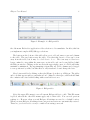
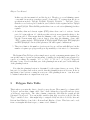
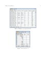
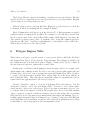
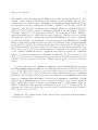
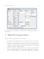
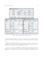
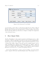
Habgen User Manual
NCASI Statistics and Model Development Group
∗
Version 2 November 15, 2005
Abstract
Habgen is a regime generator, written in Java, for Habplan. Habgen produces input
data so that Habplan can develop a management schedule for an area of land that is
divided into polygons. Typically this land area might be 100,000 acres consisting of
5000 polygons. Habgen is set up as a series of tables that the user must operate on
in a more or less sequential fashion. This setup is intended to provide a systematic
approach to generating input data for Habplan Flow components, Biological type II
components, and Block components.
∗
NCASI: http://ncasi.uml.edu/
1
Habgen User Manual
1
Contents
1
Introduction
4
2
Installation
5
3
Generic Comments about Habgen Functionality
5
4
Regime Class Table
7
5
Polygon Data Table
8
6
Polygon Regime Table
10
7
Growth Models
11
8
Habgen Flow Component Options
16
9
Flow Output Table
19
10 Biological Output Table
22
11 Block output table
25
12 Handling Large Problems
28
13 How to Add Models
28
14 Future Directions
29
Habgen User Manual
2
List of Figures
1
Example of a Habgen table . . . . . . . . . . . . . . . . . . . . . . . . . . . .
6
2
Habgen tabs . . . . . . . . . . . . . . . . . . . . . . . . . . . . . . . . . . . .
6
3
Example of a regime class table . . . . . . . . . . . . . . . . . . . . . . . . .
7
4
Example of a polygon data table
. . . . . . . . . . . . . . . . . . . . . . . .
9
5
Row selection tool . . . . . . . . . . . . . . . . . . . . . . . . . . . . . . . . .
9
6
Polygon regime table . . . . . . . . . . . . . . . . . . . . . . . . . . . . . . .
11
7
Model selection tool and setup forms . . . . . . . . . . . . . . . . . . . . . .
13
8
Setup form for PMRC model, using herbicide, bedding, fertilizer, and product
class options . . . . . . . . . . . . . . . . . . . . . . . . . . . . . . . . . . . .
16
9
Model Selection Tool and Setup forms . . . . . . . . . . . . . . . . . . . . .
18
10
Model Selection Tool for CLASS . . . . . . . . . . . . . . . . . . . . . . . . .
19
11
Example of a Flow output table . . . . . . . . . . . . . . . . . . . . . . . . .
20
12
Decay FlowTool . . . . . . . . . . . . . . . . . . . . . . . . . . . . . . . . . .
21
13
Add FlowTool . . . . . . . . . . . . . . . . . . . . . . . . . . . . . . . . . . .
21
14
Copy FlowTool . . . . . . . . . . . . . . . . . . . . . . . . . . . . . . . . . .
22
15
Bio-Output table and NPV Setup Form . . . . . . . . . . . . . . . . . . . . .
23
16
NPV Setup Form for ranking regimes according to output volume . . . . . .
25
17
NPV Setup Form for summing output volumes, with twice as much weight on
Flow 3 . . . . . . . . . . . . . . . . . . . . . . . . . . . . . . . . . . . . . . .
25
Example of block output table . . . . . . . . . . . . . . . . . . . . . . . . . .
26
18
Habgen User Manual
19
Example of nabe tool . . . . . . . . . . . . . . . . . . . . . . . . . . . . . . .
3
27
Habgen User Manual
1
4
Introduction
Habgen is a regime generator for Habplan. Habgen produces input data so that Habplan can
develop a management schedule for an area of land that is divided into polygons. Typically
this land area might be 100,000 acres consisting of 5000 polygons. Habplan develops a
schedule by selecting a single management regime for each polygon in such a way that the
user’s objectives are met in a near optimal fashion. Habplan requires the user to input,
for each polygon, a list of acceptable management regimes from which to select. A regime
consists of a string of years where management actions occur and an output for each year.
For example, polygon ”P1” could have a regime called ”TC#10#20” that thins the polygon
producing 50000 cubic feet of wood in year 10 and then clearcuts in year 20 producing another
100000 cubic feet. This would be input to a Habplan flow component as: P1 TC#10#20 10
20 50000 100000. Habgen separates action periods in a regime with a ”#”, so there is a # for
each period in the regime. For example, a 2 period regime has 2 years where actions occur.
Each polygon can have many regimes to select from, say 100. If there are 5000 polygons
you need to generate a very large input file for Habplan, e.g. with 500,000 rows. Habgen is
designed to make this task easy.
Habgen is set up as a series of tables that the user must operate on in a more or less
sequential fashion. A section is dedicated below to describing each of the Habgen tables
. This setup is intended to provide a systematic approach to generating input data for
Habplan Flow components, Biological type II components, and Block components. Regimes
are specified in the “Regime-Class” table, and polygon data are input with the “Poly-Data”
table. The “Poly-Regime” table is used to merge the regime and polygon data. Growth and
yield models are then selected to produce output from the “Poly-Regime” table. Output
data from the growth models are stored in the “Flow” table(s). Each “Flow” table could,
for example, represent a different product, e.g. sawtimber, pulpwood and chip ’n saw.
Optionally, you can write out the data in the “Poly-Regime” table, and run it through
an external growth model to produce flow data. This “Flow” data is the input data that
Habplan requires. It will be a while before Habgen includes growth models for all major
species and regions, which is the long term goal. Meanwhile, Habgen provides a means to
become familiar with how Habplan input data is generated, even if you aren’t willing to use
the models it currently includes.
The “Bio-Output” table allows the user to rank the regimes to indicate those regimes
that are more desirable to Habplan. This ranking can be done in a few different ways. One
option would be to rank regimes based on the total harvested timber volume associated
with each regime. Another option would be to rank regimes based on Net Present Value
(NPV) associated with each regime. The “Bio-Output” table creates and stores this “regime
Habgen User Manual
5
ranking data”.
The “Block” table has functionality for creating a neighbor file from an ArcView( TM )
Shapefile. This provides the neighborhood input data that Habplan requires for the Block
Component and the Spatial Model Component.
2
Installation
Habgen is written in Java, so there must be a Java Virtual Machine (Compiler) installed
on your computer in order to run it. The Habgen distribution file (habgen.jar) is a zipped
archive obtainable from the habgen download page. You’ll need a utility to unzip this
file, such as the jar utility that comes with the Java Software Development Kit (SDK).
If you have another means of unzipping the distribution file, you only need to install the
much smaller Java Runtime Environment (JRE). Obtain either the SDK or the JRE from
http://java.sun.com/j2se/.
3
Generic Comments about Habgen Functionality
All Habgen tables have much of the same functionality. Change individual cell values by
clicking on the cell and typing the value. The change won’t take effect until you move out
of the cell. Like the Regime Class Table shown below (Figure 1), tables have 3 menus. The
File menu allows you to read and write the current values of this table from or to a file. The
Edit menu lets you undo a recent change or select and unselect all rows in the table.
The Tools menu lets you open the ColumnNamesTool and the SelectionTool. As you
might expect, you can change the column names with the columnNamesTool. However, for
most tables you should use the original Habgen columnnames. Habgen figures out how to
find things in tables by looking at the column names. For example, Habgen will find the
Regime column in the RegimeClass Table by looking for the column called ”Regime”. You
might want to change names of your data columns in the Polygon Table so that growthmodels
can find the variables they need automatically.
The selection tool lets you select rows in the table based on values of variables in the
row. This can be indispensable when there are many polygons. The delete button in the
selection tool will delete all selected rows, so be careful. If you make a mistake, use undo in
Habgen User Manual
6
Figure 1: Example of a Habgen table
the edit menu. Each select application of the selection tool is cumulative. In effect, this lets
you implement complex AND/OR type selections.
The buttons at the bottom of the table allow you to add and remove rows and columns
to the table. The save button saves the table. Note that this lower tool bar can be torn
away from the table, but it may be a bad idea to do so. The torn away toolbar is no
longer confined to stay within the same space as its table, and can become hidden behind
the Habgen window. Clicking on the arrows in the upper right corner of a Table will either
maximize or minimize it. Try experimenting to figure this out. Table columns can be dragged
to new positions if you like, but this effect is only visual and doesn’t change the data.
Move between tables by clicking on the tabs (Figure 2) at the top of Habgen. The tables
and tools that appear under a particular tab are confined to that space, which should limit
the confusion associated with working with several tables at once.
Figure 2: Habgen tabs
Select the upper File menu to save all current Habgen tables to a file. This File menu
is global, whereas the other File menus apply only to their table. You can read previous
settings too. However, when you exit Habgen, all settings are saved to a default location.
When you start Habgen, all settings from your previous session are automatically restored.
Therefore, you don’t need to worry too much about saving your work.
Habgen User Manual
7
When you want to start a completely new session – clear a table by either reading in new
data, or by selecting all rows and using the delete button on the selection tool.
4
Regime Class Table
A regime class defines an array of individual regimes that are logically grouped together.
A regime class is defined by the number of action periods and the year range within each
period. The Regime-Class Table (Figure 3) allows the user to specify a name for each regime
class in column 1 and then year ranges for each period in subsequent columns. The regime
table shown below has 3 important regime classes specified:
1. The do-nothing class (DN) has year 0 specified for period1. Unless there is some
reason not to do so, every polygon should have a do-nothing regime specified as one
of its possible regimes. In this case, the RD and BP classes are do-nothings that get
assigned to roads and Borrow Pits, but they’re still do-nothings.
Figure 3: Example of a regime class table
2. A clear cut regime (CC) with an action occurring in only 1 period. The action (clearcutting) will occur in one of the these years, 1,2,3,...,15. This was succinctly specified by
giving a year range of 1-15.
3. A thinning regime (T) that allows for actions in 2 periods. These actions (thinning)
can occur in any of 15 years for period 1 crossed with 15 years for period 2. A regime
period can also specify an increment and a lag until the second period action year.
Habgen User Manual
8
In this case, the increment is 1 and the lag is 9. Therefore, a second thinning cannot
occur until 9 non-action years have passed. Some valid ”T” regimes from the above
specification include: T#1#0, T#1#10, T#2#11, T#2#12, ..., T#15#0. Notice
that the second action period starts in year 0, which creates regimes such as T#1#0
through T#15#0. This tells Habgen that there is no second action (thinning) for these
regimes.
4. A fertilize, thin and clearcut regime (FTC) where there can be 3 actions. Action
period 2 begins with an “n”, which says this action is non-sequential relative to the
previous period. This means that the thinning could occur before the fertilization,
but the clearcut must still occur at least 9 years after the thinning. Some valid
“FTC” regimes include: FTC#0#1#0, FTC#1#1#0,FTC#2#1#0, FTC#0#1#10
and FTC#10#6#15. In fact, this generates 341 valid regime combinations.
5. There is no limit to the number of action periods you could use with Habgen, but the
number of regimes per polygon will grow exponentially, so it is wise to be conservative.
The Regime-Class Table provides a simple way to specify your management regimes. You
can specifiy ranges of years and an increment, or simply give individual years separated by
a space or a comma. For example, ”1-5” or ”1-5,1” or ”1 2 3 4 5” or ”1,2,3,4,5” all specify
the same 5 years. Year 1 is the first year of the planning horizon and year 5 is the fifth year
of the planning horizon.
Note that the planning horizon is determined by the regime-classes you create. If the
last period of a regime class ends at year 30, then the planning horizon is 30 years. It also is
important to have actions occuring in every year of the planning horizon – even flow can’t
be attained unless there is output from every year.
5
Polygon Data Table
This is where you enter the data to describe your polygons. There must be a column called
”Polygon” and another column called ”Size”, that contain the polygon ID and size (acres
or hectares), respectively. The other columns contain the data that the growth models
(discussed below) need. You can include variables that help you select a model, like the
”Type” variable below – this might help to assign Loblolly models to Loblolly data and
Bottom Land Hardwood models to Bottom Land Hardwood data. This data can be read
from a rectangular file that is space, comma or tab delimited.
Habgen User Manual
9
Figure 4: Example of a polygon data table
Figure 5: Row selection tool
Habgen User Manual
10
The Polygon ID can be just about anything – use whatever is in your database. The Size
variable is needed to expand the per acre model predictions to per polygon values. Habplan
doesn’t want per acre values in the flow data.
When it’s time to select rows from this table (Figure 4), get the selection tool from the
tools menu. It will look something like the example in Figure 5.
Every Column in the table has a row in the Selection Tool. Habgen assumes a variable
is numeric unless you uncheck the checkBox. For example, to select all Pine polygons from
the above table, enter ”Pine” in the GE and LE column, which will select rows where the
Type variable is exactly equal to Pine. Not putting ”Pine” in the LE column would select
rows that are GE ”Pine” – but Type is alphanumeric so ”SweetGum” would be GE ”Pine”.
That would probably not be the desired result.
6
Polygon Regime Table
This is where you begin to reap the reward of your previous efforts to fill in the Poly-Data
and Regime-Class Tables. Notice that the Polygon-Regime Table (Figure 6) will have all
the columns from the Poly-Data Table, plus a ”Regime” column, and a ”Model” column. It
also has some new buttons to push in the bottom toolBar.
At this point, you’ll find yourself jumping between the first 3 tables on a regular basis,
which might seem confusing at first. In order to associate polygons with regimes take the
following steps: (1) select 1 or more regime-classes from the Regime-Class Table, (2) Select
1 or more polygons from the Poly-Data Table, and(3) Push one of the merge buttons on
the Poly-Regime Table. This will generate individual regimes by expanding the selected
regime-classes and applying them to the selected polygons.
Use the ”MergeNew” button to clear the Poly-Regime Table and startover. Use the
”MergeAdd” button to add to the Poly-Regime Table. You have to decide what regimeclasses should be allowed for each polygon. If you don’t want a particular polygon to ever
be clearcut, then don’t assign it a clearcut (CC) regime-class. If you don’t want anything
done to a polygon, because it contains an endangered species, then assign only a do-nothing
(DN) class. If you are doing uneven-aged management, then assign only thinning (T) or donothing regimes. Remember that do-nothings are a good thing, because they allow Habplan
greater flexibility as it is searching for solutions. Also, with a short planning horizon, it may
be unrealistic to expect all polygons to have management actions.
Habgen User Manual
11
Figure 6: Polygon regime table
Habgen gives names to individual regimes (after expanding the regime classes) by appending the action years to the regime-class name. Thus, the name ”CC#10” describes the
regime that clearcuts at year 10. Likewise ”T#10#30” means thin at years 10 and 30. These
regime-names will end up in the Habplan input data, so you need to be able to interpret
their meaning.
7
Growth Models
Habgen contains models that will grow the polygons to produce the future output that
should result if a particular management regime is followed. In theory, there is no limit
to the number of stand level growth models that Habgen can contain. Currently, Habgen
Habgen User Manual
12
includes the following models:
1. Even-aged, Natural Loblolly Pine. (Brender, E.V. and Clutter,J.L. 1970. GA Forest
Research Council Rep. No. 23). This model needs inital Age, Site Index Base Age
50, and Initial Basal Area. The model will predict cubic foot volume or basal area.
Habgen will find these variables automatically if you label the columns as Site, Age ,
andBA . This is case sensitive.
2. Old-Field Loblolly Plantations. (Burkhart, HE, Parker, RC, Strub, MR, Oderwald,
RG. 1972. Virginia Tech. Publication FWS-3-72). This model needs either Site Index
Base Age 25 or average Height of Dominants. It also needs Number of Trees Per Acre
(1-inch DBH class and above). Call these variables Site, H and N so that Habgen can
find them automatically.
3. NEW - PMRC (1996) models. These models were developed at the University of
Georgia for a region that covers the Carolinas, Georgia, Florida and Alabama. There
is one version for the Upper Coastal Plain and another for the Lower Coastal Plain.
These models require Site Index Base Age 25, number of trees and age for each stand.
Dominant height and basal area are required by the model, but can be predicted if they
aren’t available. Call these variables Site, N, Age, H and BA so Habgen will find them
automatically. The outputs that can be obtained from these models include, TVOB,
TVIB, GWOB, DWIB, N and BA.
Other models can and will be added. But we have to start somewhere. You can add
models too! This option will be discussed later in more detail.
A growth model can be applied to a polygon after it has been assigned some regimes by
following these steps:
1. On the Poly-Regime Table, first select from the Flow drop down menu which Flow
table you want output data written to, i.e. Flow 1, Flow 2, etc. (This feature is
useful for creating multiple flow components, e.g. perhaps you are interested in tracking/constraining the flow of basal area, timber volume and stem density simultaneously,
or you may want to simultaneously track/constrain the flow of different wood products,
such as sawtimber, chip-n-saw and pulpwood.)
2. Open the modelTool window by pressing the button at the bottom of the Poly-Regime
Table.
3. Select a model for each period from the modelTool.
Habgen User Manual
13
4. Press the ”Setup” button on the modelTool to control some of the model settings.
5. Press the “InitFlow” button on the Model Selection Tool, to initialize the Flow table
that you have selected (basically this just creates a placeholder in the Flow table for
every polygon-regime combination).
6. Select the rows from the Poly-Regime Table that the models should apply to.
7. Press the ”Apply” button to run the models for the selected rows. Output data will
be stored in the Flow table that you selected.
This is sounding complicated, so let’s step through the process. Figure 7 shows the
modelTool with models LobEven and LobPlant selected for periods 1 and 2, respectively.
You might do this if natural stands were to be clearcut in period 1, replanted and then the
resulting plantations would be cut in period 2. The ”Setup” buttons were pushed to open
the 2 Setup windows.
Figure 7: Model selection tool and setup forms
The Size=1 checkbox (Model Selection Tool) will cause the output to be per acre, whereas
the default is the total output per polygon. Looking at the per acre value might help you
Habgen User Manual
14
decide if the growth model is producing reasonable results, but don’t feed per acre values to
Habplan!
The Scale checkbox (Model Selection Tool) allows you to apply a scaling factor to all
output. For example, you might multiply by 31 to convert cubic feet to pounds (dry weight).
The LobEven Setup window shows that the input variables were found as ”BA”, ”Site”
and ”Age”. The selected output from the model is ”CV” for cubic volume. The ”Residual”
value is 0, which means that all Basal Area is removed. A residual of 0.5 means to leave
50% of the BA. Likewise, a value of 80 means leave 80 square feet of BA. Note: If the stand
had less than 80 square feet at the time of cutting, then nothing would be done. Remember
that the regime tells Habgen when the stand will be cut.
The ”ThresholdVar” is set to none and the Threshold value is 0. You could select BA as
the ThresholdVar and 80 as theThreshold value. In this case, Habgen outputs nothing unless
the stand has at least this much residual BA. Furthermore, when Threshold is not ”none”,
then the output is the residual currently on the stand, not the amount that was removed.
Here’s an example of how to make use of ”Thresholding”. Suppose you select ”Size” (acres)
as the output and you think that Red Cockaded Woodpeckers (RCW) can’t live in the stand
with less than a 100 square feet of BA. Setting the Threshold to 100 will cause Habgen to
output 0 when the growth model says the stand has less than 100 sq ft of BA, and it will
output the size of the stand when it exceeds 100 sq ft of BA. This creates data for a flow
component that will allow you to maintain an even flow of RCW acres. If the growth model
keeps track of average stand diameter, you could also threshold on diameter. The hope is
that thresholding allows you to schedule habitat.
Note that the Period 2 ”Setup Window” above has ignore for H, i.e. Height of Dominants.
When Habgen can’t find the column name it wants, it tries to ignore the variable. You can
select the column to use for Habgen – maybe your name was NTREES instead of N. Also,
some growth models allow for alternative input. The ”Lob Plant” or PMRC models can
either predict H from Site Index or use a measured H. If you have H in the data then
tell Habgen to ignore Site. WARNING: When variables that the model needs are ignored,
Habgen will return negative numbers. If you were applying the same growth model to both
Period 1 and Period 2 (e.g. Lob Even), a shortcut would be to configure the Period 1 Setup
window, and then press the “Copy” button. This would result in the Period 2 model having
the exact same configuration as the Period 1 model.
Habgen now has the capability to include bedding, herbicide, and fertilizer (nitrogen
and phosphorus) treatments for the PMRC models. Habgen also allows the user to specify
product classes for the PMRC models (in terms of a top diameter and dbh range). To access
Habgen User Manual
15
these features, select the appropriate PMRC model on the “Model Selection Tool”. Now
click the “Setup” button to specify the model settings. Note the “Fertilize” and “Product”
buttons next to the “Plant” button. Assuming you are wanting to plant, fertilize and specify
product classes, click all 3 of these buttons (“Plant”, “Fertilize” and “Product”). Notice the
“Herbicide” and “Bedding” checkboxes under “Planting” (Figure 8). Click the “Herbicide”
checkbox to add complete control of competing vegetation to site preparation . Click the
“Bedding” checkbox to add double-pass bedding to site preparation. Under “Fertilize”,
specify how many lbs/acre of Nitrogen you want to apply (e.g. 300 lbs/acre), and click the
“Phosphorous” checkbox to include Phosphorous with fertilization. To isolate a particular
product class, specify a “Top Diameter”, and an upper and lower DBH threshold (“DBH
Range”). Stand level growth and yield responses to both herbicide and bedding treatments
are modelled according to the growth response models developed by L. V. Pienaar and J.
W. Rheney (Modeling stand level growth and yield response to silvicultural treatments. 1995.
Forest Science 41(3): 629-638 ). Growth responses to fertilization are modelled according
to the “adjusted” PMRC models (i.e. original models adapted to include an “adjustment
term” to account for fertilization), as presented in: Harrison, W. M. and Borders, B. E.
1996. Yield prediction and growth projection for site-prepared loblolly pine plantations in the
Carolinas, Georgia, Alabama and Florida. PMRC technical report, University of Georgia,
1996-1.
A point of interest is the “unthinned counterpart” approach that Habgen uses when
modeling thinnings with the PMRC models. This approach is based on the idea, developed
by A. J. O’Conner (1935. Forest research with special reference to planting distances and
thinning. Br. Emp. For. Conf., South Africa. 30pp.), that the basal area of a thinned
plantation could be expressed as a proportion of the basal area of an unthinned stand of the
same age, dominant height and number of trees per acre (unthinned counterpart). Growth
response due to thinning, therefore, can be expressed in terms of a projected competition
index, causing the projected basal area of the thinned stand to approach that of the unthinned counterpart. This approach was further developed by L. V. Pienaar (1979. An
approximation of basal area growth after thinning based on growth in unthinned plantations.
Forest Science 25(2): 223-232 ).
Finally, the ”Info” button on the “Setup” window will pop up some written information
about the selected model.
Habgen User Manual
16
Figure 8: Setup form for PMRC model, using herbicide, bedding, fertilizer, and product
class options
8
Habgen Flow Component Options
Habgen can make the following types of flow component:
1. A normal flow component that gives the year and output for each period of the regime.
2. A habitat flow component that gives an output for each year of the planning period.
This type of flow usually produces non-zero output only if the amount of residual
vegetation exceeds some threshold. The idea is that there must be enough residual
vegetation for the stand to qualify as habitat.
3. An ending age class flow component that allows you to control the age class distribution
at the end of the planning period to assure long-term sustainability. A variation on
this is to control the distribution of last-entry times. Ending age class distribution
Habgen User Manual
17
makes sense when clearcutting is the principal management technique. Distribution
of last entry times might be useful when thinning is the management technique. This
component is made possible by using the following trick: the x-axis on the flow graph
shows the age-class and the y-axis shows acres. For all other flow components, the
x-axis is the planning period year.
Select one of the radioButtons on the Model Selection Tool shown above to control the
kind of Flow Component. Typically, the ”Norm” button is selected to get the so-called
normal flow component.
THE HABITAT RADIO BUTTON CAUSES MANY THINGS TO HAPPEN DIFFERENTLY. In particular, it adds an additional Habitat period and causes there to be output
for every year of the planning horizon, not just management action years. This is useful
for creating habitat Flow components (see the Habgen example ). By selecting the habitat
button, setting output to Size, and setting a Threshold variable, you can create a flow component that controls the number of acres of habitat according to your specifications. The
”Plant” button on the Setup Forms (Figure 9) allows you to simulate a planting immediately
after a clearcut. Here’s what you see if both ”Habitat” and ”Plant” are selected:
Notice that the Model Selection Tool has Habitat selected, which created a third ”Habitat” period. Assuming, this is a clearcut regime with only one actual management year,
the Period1 form applies to the management year, and the Habitat Setup Form (Period3)
applies to all other years. Period1 is setup to do a complete clearcut followed by a planting.
The planting will result in 1000 Trees per acre 5 years after the cutting, so if its cut in year 1
then the planting begins to ”count” at year 6 with N=1000 and Site having improved by 8%
(due to improved stock). The output is set to size and the Threshold is set to cubic volume
(CV=1000). Since there will be no residual after a clearcut, there will be no output in the
year of clearcutting, i.e. none of this type of habitat at that particular polygon. The Period3
form applies to all the other years (period 3 is the habitat period in this case). It says to
leave a residual of N=2000 – in other words you can’t cut at all. It says to output the size
of the polygon if CV is greater than or equal to 1000. The combination of the Period1 and
Period3 (Habitat) setups result in a polygon contributing to habitat before a clearcut and
sometime beyond 5 years after a clearcut when the planting has regrown. See the Habgen
example for more detail on this.
Do-Nothing Regimes are also impacted when Habitat is checked. This causes a doNothing to act like a regime with a management action in year1. Therefore, year1 for a
do-Nothing is controlled by the Period1 Setup Form and the other years are controlled by
the Habitat period Setup Form. This causes a do-Nothing regime to be able to produce
output for each of the planning horizon years. This makes sense in Habitat mode, because
Habgen User Manual
18
Figure 9: Model Selection Tool and Setup forms
doing nothing may allow Habitat to remain on the polygon for use by wildlife. One might
say that you’re getting something for nothing. See the Habgen example for more detail on
this.
THE CLASS RADIO BUTTON lets you create a flow component to control the end of
planning period age-class or time-to-last-entry distribution. Figure 10 shows what the Model
Selection Tool looks like if you select the CLASS radio button.
Now you need to specify a planting Lag, a Max class value, and whether Age at last
entry is added to the time since last entry. The Lag value allows for a planting lag – often
planting won’t occur until a year or 2 after a clearcut. The Max value causes all classes that
Habgen User Manual
19
Figure 10: Model Selection Tool for CLASS
are greater than or equal to Max to be thrown into the Max bin. For example, if Max=20
then age class 100 is set to 20 as are any ages greater than 20. If ”Age+” is not checked,
then the classes are the time since last entry. If ”Age+” is checked, then the classes are the
time since last entry plus the age at last entry. See example3 or example 4 for an application
of these different flow types.
9
Flow Output Table
The Flow Table (Figure 11) will contain the information that Habplan needs for a ”Flow
Component”. Whenever a growth model is applied to some rows in the Poly-Regime Table,
the output is added to the Flow Table. Since, several models may be used,the Flow Table is
built in a series of steps. Use the ”InitFlow” button on the Model Selection Tool to create
a new Flow Table with no outputs. Be sure that a model is eventually applied to all rows
in the Poly-Regime Table so that all rows in the Flow Table are completed. Apply any
arbitrary model (when not in Habitat mode) to ”DoNothing”regimes so they are properly
carried over to the Flow Table. The DoNothing years and outputs are always 0 (except in
Habitat mode), but they need to be generated by applying some model.
After the Flow Output Table is complete, select the”writeData” option under the File
menu to output the data in the format that Habplan wants. When prompted, choose to
Habgen User Manual
20
Figure 11: Example of a Flow output table
NOT “Put column names in row 1”. At this point, you have an input datafile for a Habplan
Flow component. You can do further editing of the flow Table after it is complete. However,
if you delete some rows and try to apply more models at the Poly-Regime Table, Habgen will
become angry when it sees that the N of Rows has been altered. It will insist on reinitializing
the Flow Table and you’d have to start over.
Notice the “Decay”, “Add” and “Copy” buttons on the bottom of the Flow table (Figure
11). The “Decay” feature allows you to apply a decay function to existing Flow data. This is
particularly useful when the Flow data represents carbon outputs. In such a case, the decay
function would compute the cumulative remaining carbon for the rest of the planning horizon.
All you have to do is press the “Decay” button, and specify the carbon half life in the window
that pops up (Figure 12). Now press the “Decay Flow” button on the Decay FlowTool, and
Habgen will compute the new input data, based on the decay funtion: (1/(1+log(2)/h))n ,
where “h” is the half life, and “n” is the number of years since the harvest.
Habgen User Manual
21
Figure 12: Decay FlowTool
The “Add” feature allows you to sum Flow outputs (e.g. Flow 1 + Flow 2). Press the
“Add” button on the Flow Table. This will pop up the Add FlowTools window (Figure
13). Now specify which Flow component (e.g. Flow 2) you wish to add to the current Flow
component (e.g. Flow 1), and specify what weight you want to apply to the selected Flow
(e.g. a weight of 1 would equate to Flow 1 + Flow 2, whereas a weight of 2 would equate
to Flow1 + 2 x Flow 2). Next press “Add” on the FlowTools window, and the resulting
data will be output in the current Flow table. For example if Flow 1 is decayed product
carbon and Flow 2 is residual carbon, then adding them results in total carbon on the
land and in products. You can also add the current Flow to itself, multiplied by a weight.
For example, suppose the current Flow is Flow 1, and you select Flow 1 on the FlowTools
window. Specifying a weight of 0.2, would result in Flow 1 being increased by 20%. This
“Add” feature can be used in many ways, and adds flexibility to Habgen. NOTE: When
adding tables with different numbers of output years, the table with fewer columns must be
added to a table with more (or equal) columns.
Figure 13: Add FlowTool
The “Copy” feature allows you to copy output data from one Flow table into another
Flow table. For example, assume you are currently working on the Flow 2 table, and you
want to copy the Flow 1 output data into Flow 2. Press the “Copy” button on the Flow
Table. This will pop up the Copy FlowTools window (Figure 14). Now specify which Flow
component (e.g. Flow 1) you wish to copy to the current Flow component (e.g. Flow 2), and
Habgen User Manual
22
press “Copy” on the FlowTools button. The output data from Flow 1 should now appear in
the Flow 2 table.
Figure 14: Copy FlowTool
Remember that you can write out the data from the Poly-Regime Table to a file and run
it through your own growth routines if Habgen doesn’t contain the growth models you need.
It should be relatively easy to batch process the Polygon-Regime data and turn it into flow
data without using Habgen.
10
Biological Output Table
The Biological component in Habplan allows the user to rank regimes by order of importance. This ranking scheme could, for instance, be based on Net Present Value (NPV) or
total harvested volume associated with each regime. The purpose of this Biological component is to bias the Habplan scheduler toward assigning the regime that produces the most
NPV/volume for each stand. The ranks can be arbitrarily chosen, and only the ordering
matters, not the magnitude. So If polygon P1 has 2 allowed regimes (R1 and R2) then the
following Biological data says R2 is better than R1:
P1 R1 2
P1 R2 2.1
The only thing that matters is that 2.1 is bigger than 2 – ranks of 1 and 50 would yield the
same result. We shall consider two methods for ranking regimes: 1) NPV (or LEV) and 2)
Total harvested volume.
To create this “ranking data”, use the “NPV” feature on the Bio-Output Table (Figure
15). Access this feature by pressing the “NPV” button on the Bio-Output Table. Before
proceeding, initialize the Bio-Output Table by pressing the “Init” button on the bottom of
the table. This initialization process creates a placeholder in the Bio-Output Table for every
polygon-regime combination, which now allows you the option of using the “Row Selection
Habgen User Manual
23
Tool” (under “Tools”) to select specific rows when computing NPV or LEV. This enables
you to change the value or cost settings for different regimes, e.g. land sale regimes might
have a negative cost, representing land sale revenue, which is specific only to the land sale
regime. Also note that the user can select (Value Setup Form) between calculating Net
Present Values (NPV) and Land Expectation Values (LEV). LEV is essentially the NPV for
an infinite time horizon (i.e. multiple rotations).
Figure 15: Bio-Output table and NPV Setup Form
Habgen User Manual
24
Now, to rank regimes by NPV, enter per unit product prices for the respective Flow
components in the Value Setup Form (for example, assume Flow 1 = pulpwood, Flow 2 =
chip-n-saw andFlow 3 = sawtimber). Also enter an interest rate.
If there are costs associated with various regimes, press the “Cost” button on the NPV
Setup Form to open the Costs Table (Figure 15). Notice that the Costs Table has the same
rows and columns as the Regime Class Table. Costs can vary by regime and action period,
and are entered into the Cost Table. Costs are per acre and you must specify the name of
the acreage column at the bottom of the costs table unless the name is ”Size”. The acreages
come from the Poly-Regime Table, which must have the same number of rows as the Flow
tables or you will get an error message. Now, once the NPV and Costs Tables are filled out,
press the “Calculate” button on the NPV Setup Form to compute the value column in the
Bio-Output Table (Figure 15). Note that if you have not selected specific rows from the BioOutput Table to which the NPV computations should apply, upon pressing “Calculate”, a
window will pop up confirming that you want to apply the NPV computations to all rows in
the Bio-Output Table. If this is the case, click “OK”. Otherwise, click “Cancel” and select
the rows of interest. The costs are discounted and then substracted from the discounted
revenues for each polygon and regime. This assumes that the 3 Flow tables are compatible,
i.e. they contain the same regimes and output years. If a table is not compatible, it is
skipped. To rank the regimes by total output volume, ignore the Costs Table, and simply
set all the Flow Values on the NPV Setup Form to 1, and the interest rate to 0 (Figure
16). Now, upon pressing the “Calculate” button, the Flow outputs are summed for each
polygon-regime combination (i.e. Flow 1 + Flow 2 + Flow 3). If, for some reason, you
wanted to put more weight on the Flow 3 outputs, you could, for example, give Flow 1 and
2 a value of 1, and Flow 3 a value of 2 (i.e. twice as much weight as Flows 1 & 2). As long as
you set the interest rate to 0, the NPV function becomes a simple summing function (Figure
17).
The Biological Output Table can now be written to a file (commonly named Bio2.data)
and read by Habplan (use the Table’s File menu).
Remember that allowed regimes in Habplan are determined by finding the intersection of
a polygon’s allowed regimes for each Flow and Biological Type II component. The default
Biological Output Table will have all regimes found in the Flow Output Table. However, you
can delete Biological Output rows if you want to eliminate some regimes from consideration
for particular polygons.
Habgen User Manual
25
Figure 16: NPV Setup Form for ranking regimes according to output volume
Figure 17: NPV Setup Form for summing output volumes, with twice as much weight on
Flow 3
11
Block output table
This section of Habgen allows you to create the neighbor input data required for a Habplan
Block Component. You will need to have an ArcView ShapeFile available that corresponds
to the Poly-Data Table. In other words, there must be a one-to-one correspondence between
the polygons in the ShapeFile and each row of the polygon data table. The first step is to
open the NabeTool by pressing the button at the bottom of the Block Output Table shown
in Figure 18. The NabeTool looks like the example shown in Figure 19.
Habgen User Manual
26
Figure 18: Example of block output table
Press the ”FindFile” button to locate your ArcView Shapefile. Then press the ”ReadPolys” button to read the shapefile. You will receive a report about how many Polygons
were read. Note that only a shapefile containing polygons will work here. ShapeFiles can
contain various other entities, but Habgen only needs to know about polygons.
Now you’ve read the shapefile and also have read the polygon data into the Poly-Data
Table. The next move will be to press the ”Apply” button to start one of the neighbor
finding algorithms. However, the NabeTool will need to locate 2 columns in the Poly-Data
Table: 1) A column called ”Polygon” that gives the polygon ID, and 2) A column called
”Size” that gives the size of the polygon in acres, hectares or whatever. If NabeTool doesn’t
find columns with these exact names, it will ask you what they are called. So to avoid this
additional request for input, you might want to name those 2 columns in the Poly-Data
Table as follows: ”Polygon” and ”Size”.
Habgen User Manual
27
Figure 19: Example of nabe tool
There are 2 basic neighbor finding methods available in the NabeTool:
1. The default selection is ”Adjacent”, which chooses neighbors that are immediately
adjacent to the target polygon. The ”Adjacent” method also includes the option of
specifying a proportion of shared boundary. The default proportion is 0, so polygons
that touch at even a single point are neighbors. If the proportion is increased, then
the shared boundary must be at least as great as the specified proportion. The shared
proportion computation is based on the sum of the perimeters of the 2 polygons being
considered. Move the slider to select the desired limiting proportion. Note that placing
the mouse pointer over the slider will cause the current slider setting to be displayed.
2. The ”Buffer” option will allow you find neighbors based on a specified buffer width.
This means that any polygon within the buffer distance becomes a neighbor. Just
fill in the TextField next to the Buffer button to specify the buffer width. Using
buffer width=0 gives the same result as the ”Adjacent” option with shared boundary
proportion=0.
The neighbor-finding algorithm is reasonably efficient, but it may still take several minutes to finish when thousands of polygons are involved. At the end, the Block Output Table
contains the data that Habplan needs for a blocksize objective function component. Save
this data by selecting ”WriteData” from the ”File” menu on the Block Table.
Habgen User Manual
12
28
Handling Large Problems
Habgen creates a number of tables that can have many rows for large problems. Suppose
you have 5000 polygons with 100 regimes per polygon. Then there will be 500,000 rows in
the following tables: Polygon-Regime Table, Flow Output Table, and the Biological Output
Table. All this is held in memory, so you could find your computer chugging away for a long
time when you start or exit Habgen, because its either reading all this data or trying to save
it. Consider the following tips:
1. Its important to start Habgen so it has access to plenty of memory like this:
java -mx256m Habgen1
This gives Habgen access to 256 MB of RAM if it needs it. Java, by default limits each
program to 16MB of RAM.
2. After creating a table, save it using the tables file menu and the writedata option. This
allows you to save the table in a tab delimited ascii file. Then if anything goes wrong,
you can start Habgen and read this file using File - readdata.
3. When you exit Habgen using the File - Exit option, Habgen saves all Tables and
other settings to the file Habgen1/hbg/habgenSettings.hbg. When Habgen starts, it
reads this file to restore all settings and tables from the previous run. If this file gets
corrupted, then Habgen won’t start properly. The best solution if this occurs is to
delete the ”habgenSettings.hbg” file. Then start Habgen and read in the ascii versions
of the tables that you saved according to item 2 above. You can restore original column
names using the column names tool.
4. With large problems, it will take some time for Habgen to exit and to start, because its
writing or reading lots of data. You can speed this up by clearing large tables before
you exit. Save the table using File - writedata first, so you can recover it later. Clear
a table by selecting all rows, then hit the delete button on the selection tool.
13
How to Add Models
The source code for the models is included in the Habgen/growthmodels directory. All files
that are required for changing models are found in this directory. This allows you to look at
the code to determine how the model works and if it does what you think it should. You can
also create your own models by extending the AbstractYieldModel class if you want to do
Habgen User Manual
29
some Java programming. If you do add models,please send them to ncasi so that others can
use them too. The rest of this section attempts to give a programmer enough information
to add a model to Habgen. It’s not that easy to add a model from scratch, but you could
modify one of the pre-existing existing models quite easily.
Step 1 is to look at the javadoc output for other models. YieldModel1.java and YieldModel2.java are the Brender and Clutter,and Burkhart et al models. The PMRC models
are in PmrcLCP.java and PmrcUCP.java. You will need to create a class similar to these
for the model you wish to add. Your class must extend AbstractYieldModel and implement
each of its methods. The most important method is grow(), which grows all of the required
variables according to your model. You can add new methods to do things internally for
your model, but you must extend AbstractYieldModel and implement the methods that it
contains.
All of the growth model related classes are part of the growthmodel package within
Habgen. You can compile your new growthmodel class which you might name BestModel.java
from the Habgen1 directory as follows:
javac growthmodel/BestModel.java
Don’t try to compile from the ”growthmodel” directory or java gets confused about where
to find the growthmodel package. You’ll need the complete java software development kit
installed to do this, but you probably have that if you are running Habgen. You’ll also need
a text or program editor.
Now you have to let Habgen know about your new model. You can add BestModel to
Habgen by editing the buildModels() method in ModelConfigurator.java. Then compile this
as follows:
javac growthmodel/ModelConfigurator.java
14
Future Directions
1) Add more models.