Download Finding linear correlations in the data of the nTOF facility

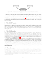
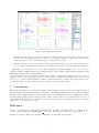
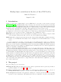
Finding linear correlations in the data of the nTOF facility
Emilio Del Tessandoro
August 16, 2013
1
Introduction
nTOF is a neutron time of flight facility located at CERN aimed to the study of neutron induced reactions
[Guerrero et al. (2013)]. An high intensity neutron beam is produced from the reactions caused by an incoming
proton pulse that hits a lead spallation target. The experimental area is located approximately 180m away from
the spallation target. This flight path basically allows to compute the kinetic energy of the neutrons based their
arrival time at the experimental area, allowing to fully characterize the produced neutron beam.
The aim of the experiment is to measure with very high precision the cross sections of specific reactions, like
for example the cross section for neutron capture (n, γ), or fission (n, f ). Clearly different experiments require
different kind of detectors but it’s possible to classify all the data of nTOF in two classes:
FAST data that is coming the detectors. It is sampled at very high speeds (order of nanoseconds) and consists
of the raw signal coming from the AD converters of the data acquisition system (DAQ).
SLOW data that is coming from sensors in various points of interest in the facility (like for example temperature,
pressure, etc). Normally this data is sampled orders of magnitude slower than the FAST data, i.e. seconds
or more.
So in the following the focus will be on the data, since it’s the main ingredient of this project. When the
experiment is running, the data acquisition system (DAQ) stores all the information coming from the detectors
firstly on a local cache and then on CASTOR (the advanced storing facility at CERN). The SLOW data instead
is handled separately and it is available in a MySQL database at ntofdaq.cern.ch. A dedicated application is
taking care of updating constantly this database.
Each experiment is subdivided in runs, that are stored as streams. Each stream contains the data of some
of the detectors (and this assignment is statically chosen before running the experiment, not dynamically by the
DAQ). Every stream may be partitioned in various segments, that are created when the data of a detector reaches
a certain size limit. Reaching this limit causes all the streams to be saved incrementally in a new segment. Since
during a run there are many incoming proton pulses, inside each segment the data is organized into events, that
correspond indeed to an incoming proton pulse. An event starts with the triggering of the correspondent detector
and finishes after a certain amount of time (order of tens of milliseconds). For space reasons, also if the whole
time is sampled by the detectors, only the interesting portions of each event are actually stored. In particular
each event is divided into signals, that are contiguous intervals of time that should be significant, e.g. because
they contain a signal peak.
2
The project
The goals of this project are at least three:
Collecting the data This part includes the retrieval of all the experimental data in a given temporal window
specified at runtime. See sections 3 and 4 for details.
Find linear correlations This part aims to find linear correlations between different measures, e.g. the proton
intensity with the number of peaks recorded by a detector. This is discussed in section 6.
Learn and report The final aim of the application, learning the correlation patterns and report if something
is going out of the normal ranges. Unfortunately there was not enough time to properly develop this part.
1
SLOW Reader
FAST Reader
Correlator
GUI
Figure 1: The thread structure of the application, where the arrows indicate data transfers.
This has been realized in a single application running various threads. This is feasible because the computations to execute are not really CPU intensive, at least in this initial stage. If in the future the application has
to be used with a very higher load, it can be split into processes (instead of threads) basically maintaining the
same design.
The structure of the final application is represented in figure 1. The main component is the correlator and GUI
thread, that also to store all the gathered data in the proper data structures. Any possible correlation between
the data is updated and computed by the threads that actually read and insert the data into the correlator (that
is the two readers).
3
The SLOW reader
There is not much to say about this component since it simply consists in a SQL client that sends queries to the
nTOF database. The filtering of the interesting data, that is obtaining only the information included in time
window, clearly is directly done through the SQL query, therefore no unnecessary network communications are
made. A read only user ntof has been set up in the MySQL database, and can access remotely the database
without password.
4
The FAST reader
This component instead is much more complicated because it has to deal with two aspect. The former is to
download the data from CASTOR, while the latter is to analyze this data on the fly (rather than store it,
for example) and immediately get some summarized information to be used in the rest of the program. This
information is related to the number of peaks that appear in the raw signal coming from the detectors (since a peak
ideally is related to some reaction that is happening). Therefore a simple peak analyzer has been implemented
to solve this purpose, as explained in section 4.1.
To get the data from CASTOR instead has been used the code of a well know program in the collaboration
(the RawReader class). At the end we realized that this code is not sufficient for handling all the informations
stored in the raw files. In fact we would need also the timestamps that correspond to each event (in every run).
At present, the application is collapsing all the informations of a run in the timestamp corresponding to its
beginning. With the informations about the time of the events we would have much more high time resolution.
As mentioned before, the FAST reader also make use of a local database that contains the creation times of
the files present in the CASTOR directories for the nTOF experiment. This little database has been built using
a python script that runs properly the nsls and xrd commands. Each line present in it has the format RUN TIME
TOTALSEGMENTS PATH.
4.1
The peak analyzer
Designing a single peak analyzer for all the detectors available at nTOF is at least a challenging job. This has
been done trying to avoid any specific value or derivative threshold but instead searching for peaks in relative
terms. For example, a condition to take into account can be to consider if the value goes outside ±3σ for a
candidate peak, where σ clearly is calculated for the current signal (detector).
Inside the peak analyzer everything is decided mainly looking at four variables, computed as exponential
weighted moving averages:
2
START
BASELINE
GAMMA
FLASH
PEAK
RECORDING
Figure 2: The states of the peak analyzer.
1. the baseline (and its variance) that is the average value coming from the current signal, when no peak is
happening.
2. the derivative (and its variance) that is the average derivative for every time interval ∆t1 , still when no
peak is happening.
Knowing these values for a “idle” situation is possible to decide if something different is happening (that
maybe is a peak). The logic of the peak analyzer is pictured in figure 2. An initial phase of “warm up” is
executed in order to initialize properly all needed variables. In this phase it is also dediced which kind of detector
we are treating (positive or negative). After this stage we enter the BASELINE state where, after updating
the four variables discussed above we check for big changes in the derivative2 . If this is the case we enter
in the PEAK RECORDING state where all the incoming values are stored for further processing (mainly for
integral and minimum or maximum calculation). In this situation the baseline and the derivative averages are
not updated. At the end, when the value come again reasonably close to the baseline, we decide if what we saw
was a peak or not. If it wasn’t the recorded values participate to updating the baseline and the derivative. In
any case we go back to the BASELINE state.
An additional state, GAMMA FLASH, is present in order to get some information about the γ-flash phenomena. The problem is that its shape can be completely different from one detector to the other, therefore this
aspect may need further investigation. This is also why I think that a good option for further development is to
use this class as a base and extend it (in terms of OOP) to specialized classes for each detector.
5
The GUI
The Graphical User Interface has been realized using the root GUI module. It’s easier to describe it with a
picture of the result, rather than words, so see figure 3.
6
Finding linear correlations
This part tries to decide if two measures f (t) and g(t), are correlated. We started searching for linear correlations,
computing a linear fit of f (t) against g(t), using the least squares method. This results in two coefficients a and b
such that a · g(t) + b is close as possible to f (t). Doing the same for g(t) against g(t), we get other two coefficients
c and d where, if the two functions are correlated we should have a · c ≈ 1. Therefore we can simplify this problem
into computing this number, having as input the data from two detectors.
While this is relatively easy, there are some problems getting adequate points f (t) and g(t) as input for the
correlation test. I remember in fact that what has been said above is meaningful if the two functions are sampled
in the same points t1 , t2 , . . . , tn . In particular we encountered two major problems in this part:
1 The
2 This
resolution of the detector.
changing of state could also be triggerd by a big change in the value.
3
Figure 3: The graphical user interface.
1. The time interval of the two input detectors may be different, therefore it’s necessary to find some intersection before calculating any correlation. Moreover one wants probably to compute the correlation only
on the last window of T seconds in the data, not on the full detector data.
2. The time resolution of the detectors can be different and in many cases is not even constant. Therefore we
need to compute some kind of interpolations to actually have the values of f (t) and g(t) in the same times.
While these two aspects have been solved without making any further assumption, the code needs some
additional testing. Assuming that the data coming from the readers is sampled in the same time instants, would
significantly simplify (and accelerate) this part.
At the end the computed correlation coefficients are stored into a variable size matrix C (because the detectors
number is not fixed at compile time) where the element C[i][j] contains the fit results for the ordered pair of
detectors (i, j); in this environment what we want to check is if the linear coefficient C[i][j] is the inverse of the
one in C[j][i]. This correlation matrix is a member variable of the correlator class.
7
Conclusions
This is just a starting point for a full online analysis of the existing correlations in the data, but the structure of
the final application should help the future development. Some further assumptions on the data, like for example
having the same sampling times for every incoming detector, may simplify the code a lot, making it also faster,
but this requires additional efforts in the reading routines. Also the future development should be moved on
“safer” frameworks than root (for example in terms of memory leaks in the graphical interface), but anyway
what has been done is a nice prototype.
References
Guerrero, C., Tsinganis, A., Berthoumieux, E., Barbagallo, M., Belloni, F., Gunsing, F., et al. (2013). Performance of the neutron time-of-flight facility n tof at cern. The European Physical Journal A, 49 (2), 1-15.
Onuchin, V., Aaij, R., Antcheva, I., Schaile, O., Barrand, G., & Bertini, D. (1995-2013).
4
A quick User Manual
The whole application has been written in C++ making use of the C++11 conveniences, mainly for the multithreading. As additional dependencies are only the boost libraries for handling the program options, the CERN root
library3 for the graphical interface and MySQL for reading the SLOW database. Since both boost and root are
already installed on lxplus, the only library that should be installed is MySQL, but instead it is simply included
in the source code since it consists of few files.
The compilation is quite simple thanks to the use of CMake, that takes care of all the needed steps, including
the addition of the library and include paths and the also the LD LIBRARY PATH setting. Therefore no special
environment configuration is needed for running the application, except for the CASTOR variables. CMake also
create the dictionary of the functions in the graphical interface using rootcint, dictionary that is needed in order
to make the signal-slot mechanism work [Onuchin et al. (1995-2013)]. For example, assuming that the source
code is present in a directory called ./source it is sufficient to type:
cmake ./source
make
And an executable called main will be produced in the current directory. The usage is quite self explanatory
(just type ./main --help to get a little help message), and only three arguments are strictly required: the
starting time, the ending time and the location of the local database. The format of the time strings can be
specified with the --format option according to the C99 strftime() function. For example this command
download and analyze the data from 24th October to the 27th, using the default time format:
./main --start "24/10/2012 00:00"
--end "27/10/2012 00:00"
--localdb ../project/NTOFDB
To create the local databese a script called createdb.py is available in the main directory. It requires no
arguments and eventually prints on stderr warnings and errors during the execution, together with a small
progress bar for each directory that is analyzed. The output instead is printed on stdout, therefore to recreate
the local database NTOFDB the following commands are needed:
./createdb.py > NTOFDB.unsorted
sort -g -k2 NTOFDB.unsorted > NTOFDB
The last command simply sorts the lines of the file based on creation time, that is the second field in the
output.
3 Version
5.34.03 for 64 bit architecture.
5