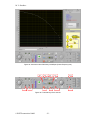
1
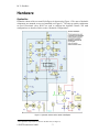
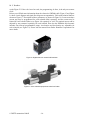
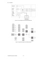
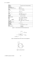
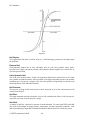
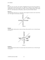
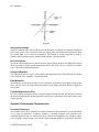
ValveExpert
Check / Adjust / Repair
Servo- and Proportional Valves
Automatic Test Stand
M. V. Shashkov
Contents
INTRODUCTION ......................................................................................... 4 REVIEW OF SPECIFICATIONS ................................................................. 5 APPLICATIONS ................................................................................................................. 5 CONTROL SIGNALS .......................................................................................................... 5 AMPLIFIER FOR PROPORTIONAL DIRECTIONAL CONTROL VALVES ...................................... 5 SPOOL POSITION SIGNALS (FEEDBACK)............................................................................ 5 ELECTRIC POWER SUPPLY FOR SERVOVALVE ................................................................... 5 HYDRAULIC FLUID ............................................................................................................ 5 HYDRAULIC POWER SUPPLY............................................................................................. 5 HARDWARE ............................................................................................... 7 HYDRAULICS.................................................................................................................... 7 WATER COOLING ............................................................................................................. 9 ELECTRIC POWER SUPPLY ............................................................................................... 9 INTERFACE ELECTRONICS .............................................................................................. 11 ALARM INDICATORS OF THE ELECTRONICS ...................................................................... 12 COMPUTER SUBSYSTEM ................................................................................................. 13 MOTOR ELECTRONICS .................................................................................................... 14 DATA ACQUISITION ELECTRONICS .................................................................................. 15 AMPLIFIER FOR PROPORTIONAL DIRECTIONAL CONTROL VALVES .................................... 15 SERVOVALVE INSTALLATION ........................................................................................... 19 SOFTWARE .............................................................................................. 22 VIRTUAL LABORATORY VALVEEXPERT............................................................................ 22 HYDRAULIC POWER SUPPLY........................................................................................... 24 UNIVERSAL AMPLIFIER ................................................................................................... 25 THE MAIN CONTROLS .................................................................................................... 25 HYDRAULIC CONFIGURATIONS ........................................................................................ 26 MEASUREMENT INSTRUMENTS ........................................................................................ 27 SETTINGS FOR THE AUTOMATIC TEST ............................................................................. 28 BIAS ADJUSTMENT......................................................................................................... 30 AUTOMATIC TEST........................................................................................................... 31 PRELIMINARY ANALYSIS ................................................................................................. 32 PRINTOUT OF THE RESULTS ............................................................................................ 32 STRUCTURE OF THE REPORT FILE................................................................................... 40 CALIBRATION ................................................................................................................. 40 MATHEMATICAL ANALYSIS................................................................... 41 LINEAR ANALYSIS .......................................................................................................... 41 FREQUENCY RESPONSE ANALYSIS ................................................................................. 42 STEP RESPONSE ANALYSIS ............................................................................................ 44 EXCEL FILE WITH RESULTS .................................................................. 45 GENERAL INFORMATION (EXCEL SHEET “MAIN”) ............................................................ 45 PRESSURE/LEAKAGE TEST (EXCEL SHEET “PRESSURE”) ............................................... 45 FLOW AB TEST (EXCEL SHEET “FLOW AB”) .................................................................. 48 FLOW A TEST (EXCEL SHEET “FLOW A”) ....................................................................... 49 FLOW B TEST (EXCEL SHEET “FLOW B”) ....................................................................... 50 © DIETZ automation GmbH
-2-
M. V. Shashkov
DYNAMIC TEST (EXCEL SHEET “DYNAMICS”) .................................................................. 51 STEP RESPONSE TEST (EXCEL SHEET “STEP”) .............................................................. 52 SAFE FLOW TEST (EXCEL SHEET “SAFE”) ...................................................................... 52 SAE RECOMMENDED TERMINOLOGY .................................................. 53 SERVOVALVE, DIRECT DRIVE FLOW-CONTROL ................................................................ 53 ELECTRICAL CHARACTERISTICS...................................................................................... 54 STATIC PERFORMANCE CHARACTERISTICS...................................................................... 55 DYNAMIC PERFORMANCE CHARACTERISTICS .................................................................. 62 © DIETZ automation GmbH
-3-
M. V. Shashkov
Introduction
ValveExpert is an automatic test stand for checking, maintenance, and adjustment of servo- and
proportional valves. This test equipment is developed in accordance to the specification of the
Parker Hannifin Corporation® and satisfies the standards established in SAE ARP 490 and ARP
4904.1 Below are the main features.
•
•
•
•
•
•
•
•
•
•
•
•
•
•
•
•
•
Wide range of servo- and proportional valves is supported. Testing flow is up to 80
L/min (21 Gal/min) and working pressure is up to 350 bar (5000 PSI).
Compact high efficient and low noise 30kW hydraulic power station is already inside.2
Temperature control system stabilizes the oil temperature in a specified range with
tolerance ±2°C.3
The integrated 3μ filtration system achieves a cleanliness level 5 of NAS1638 (level
14/11 of ISO4406) or better.
An additional, the “last chance” 10μ filter protects the valve from contamination.
Extremely robust construction of the stand. The most of hydraulic components are
mounted on one steel manifold. The only top quality components are used.
Multi-level alarm system protects the operator from risky conditions. This system
informs the operator if service is required.
Different hydraulic liquids can be used.4
The computer subsystem is based on the Intel Core2 Duo E6600 processor, 1GB RAM
and 16 bit high speed digital acquisition card NI PCIe-6259.5
The computer interface is intuitively clear and simple. Special education and knowledge
are not required. Operator works with a powerful virtual hydraulic laboratory on a 19inch touch-screen monitor.
Internal user-defined database keeps all test parameters. This database contains also
overlay polylines for automated pass/fail evaluation. The operator can use keyboard,
touch screen monitor, touch pad panel or even bar-cod scanner for fast access to the
database.
The system supports manual and automatic modes.
The measurement data includes the most of static and dynamical characteristics. Up to 15
different graphs can be obtained during one automatic test.
Complete test requires about 5 minutes. Computer shows the results during the testing
process.
A powerful mathematical analysis of the results is already embedded into the system. The
ValveExpert program saves the data in a standard MS Excel file and Excel tools can be
used for an additional analysis. The operator can use template files to prepare the printout
forms.
ValveExpert can work with any measurement units, i.e. the operator can decide which
units he will use for pressure, flow, temperature and so on.
High precision measurement tools are used. All instruments are individually calibrated
and scaled. Nonlinear calibration allows to compensate nonlinearity of transducers and to
obtain unbelievable precision.
1
The general ideas which are used in the stand can be found in http://arxiv.org/abs/math/0202070.
This hydraulic station requires three-phase 380-500V, 80A electric power supply connection. Power can be
increased up to 38kW.
3
Water connection for cooling is required.
4
Aerospace hydraulic fluids like Skydrol, Hyjet or similar require modifications in the construction of the test stand.
5
Detailed info on NI PCIe-6259 see in http://sine.ni.com/nips/cds/view/p/lang/en/nid/201814
2
© DIETZ automation GmbH
-4-
M. V. Shashkov
•
Calibration process is very simple and can be made by the operator. The only standard
measurement tools are required.
Review of Specifications
Applications
Test stand ValveExpert is developed for checking, maintenance and adjustment of four way
servo- and proportional valves.6 Working pressure of the stand is up to 350 bar (5000 PSI) and it
allows to test flow up to 80 L/min (21 Gal/min).
Control Signals
A servo- or proportional valve under testing can be controlled by voltage or current command
signal. There are five ranges for control signal: ±10V, ±10mA, ±20mA, ± 50mA and ±100mA.
Some high current servo- and proportional valves may require a special external current
amplifier.7 The build in relays can change polarity of control signal and the coil configurations
(for two coil electric servo- or proportional valves): Series, Parallel, Coil No.1 and Coil No.2.
Amplifier for Proportional Directional Control Valves
In additional to the standard Voltage/Current amplifier, the system has a programmable PWM
current amplifier PWD 00A-400 form Parker Hannifin Corporation®. This electronics can drive
most of two or one coils proportional directional control valves without position feedback and
with maximal current up to 3.5A. All parameters can be adjusted via ValveExpert software.
Spool Position Signals (Feedback)
The most of modern servo- or proportional valves have a build in electronics. These valves are
usually equipped by spool position transducers. ValveExpert can check the signal from such a
transducer. The standard signal ranges ±10V, ±10mA, ±20mA, 4–20mA are supported.
Electric Power Supply for Servovalve
Servovalves with build in electronics require external power supplies. In the most cases, it is
±15V or 24V. Such power suppliers are built in the test stand.8
Hydraulic Fluid
The test stand ValveExpert was developed and tested for a mineral oil with viscosity about 30
cSt. We recommend you to use Mobil DTE24, Shell Tellus 29, MIL-H-5606, MIL-H-83282,
MIL-H-87257 or oil with the similar parameters. Note that aerospace hydraulic fluids like
Skydrol or Hyjet® require modifications in the stand construction. The integrated filtration
system achieves a cleanliness level 5 of NAS1638 (level 14/11 of ISO4406) or better. The
capacity of the oil tank is about 100L (26Gal).
Hydraulic Power Supply
The test stand does not require an external hydraulic power supply. A modern high efficient and
low noise 30kW hydraulic power station is already inside! Maximal flow of the power station is
80 L/min (21 Gal/min) and working pressure is up to 350 bar (5000 PSI). The integrated
hydraulic power pack requires three-phase 380-500V, 80A electric power supply connection and
6
Additional adaptor manifolds allow to use this test equipment for different purposes.
Type of amplifier depends of the servo valve.
8
Maximal current is 1A for ±15V and 5A for the power supply 24V.
7
© DIETZ automation GmbH
-5-
M. V. Shashkov
a water connection for cooling. Note, the temperature control system allows to stabilize the oil
temperature in a specified range with tolerance ±2°C.
© DIETZ automation GmbH
-6-
M. V. Shashkov
Hardware
Hydraulics
Hydraulic schema of the test stand ValveExpert is shown on the Figure 1. The most of hydraulic
components are mounted on one steel manifold (see Figure 2).9 The only top quality components
are used. Directional valves K1-K7 are used to configure the hydraulic schema. The main
configurations are described in the section “Hydraulic Configurations”.
Figure 1. Hydraulic schema of the stand ValveExpert
9
These hydraulic components are shown in the blue area (see Figure 1).
© DIETZ automation GmbH
-7-
M. V. Shashkov
Pressure
transdsucer
Valve
Minimess
Flowmeter
Accumulator
10µ oil filter
Figure 2. The most of hydraulic components are mounted on one steel manifold
Hydraulic power pack (see Figure 3) uses a low noise internal gear pump and a brushless motor
with variable rotation frequency. Maximal power of the hydraulic system depends of the motor
electronics and can be up to 38kW. Maximal working pressure is 350bar (5000PSI). Maximal
flow is 80L/min (21 Gal/min).
Motor fan
Electronics for
600W motor
38kW motor
Heat exchanger
for water cooling
Oil level
transducer
Temperatire
transducer
600W motor
Water valve
Air filter
100L oil tank
3µ oil filter
Figure 3. Hydraulic power pack.
© DIETZ automation GmbH
-8-
M. V. Shashkov
Water Cooling
„Last chance“
3 µ filter
Water connection
Figure 4. Industrial water connection for cooling of the oil
Electric Power Supply
Electric schema of the stand is shown below (see Figure 5). Figure 6 and Figure 7 show electric
power distribution on the stand.
Figure 5. Electric schema of the stand
© DIETZ automation GmbH
-9-
M. V. Shashkov
L1
L2
L3
N
GND
Figure 6. ValveExpert requires three phase 380-500V, 80A electric power supply
3x400V connection
Power motor
electronics
Power motor
relay
Main fuse for
power motor
Main fuse for the
electronics, small
motor and heater
Master-slave
socket
Figure 7. Electric distribution
© DIETZ automation GmbH
-10-
M. V. Shashkov
Interface Electronics
Power supply:
±15V, ±30V, +24V
Servovale
Valve K1
Reserved
Valve K2
Valve K3
Valve K4
Reserved
Valve K5
Oil temperatuire
Valve K6
Heater
Oil level
On/Off Servovalve
Reserved
Alarm Indicator
Cooler
Reserved
Pb transducer
Pa transducer
NI connector 1
Frequency
response cylinder
Ps transducer
Reserved
Reserved
NI connector 0
Flow meter
Emergency
Filter 10µ
Filter 3µ
Alarm indicators
Frequency for
small motor
Power motor control
On/Off power motor
Figure 8. Interface electronics of the test stand ValveExpert
© DIETZ automation GmbH
-11-
M. V. Shashkov
Alarm Indicators of the Electronics
Multi-level alarm system protects the operator from risky conditions. This system informs the
operator if service is required. The program ValveExpert analyses transducers data and will
immediately stop testing if there is a problem (see page 24). The hardware alarm level is
supported by the electronics ValveExpert. It has four alarm state indicators (see Figure 8). They
are blinking if there is a problem. Figure 9 shows the possible alarm states.
Figure 9. List of possible values for the alarm indicators on the electronics
© DIETZ automation GmbH
-12-
M. V. Shashkov
Computer Subsystem
The computer subsystem is based on Intel Core2 Duo E6600 processor, 1GB RAM and 16 bit
high speed digital acquisition card NI PCIe-6259. The system includes a 19” touch screen
monitor, a stainless steel keyboard with touch pad and a bar-code scanner (see Figure 10).
Software includes Windows XP operation system, drivers, MS Excel and ValveExpert program.
Figure 10. Touch screen monitor, keyboard with touch pad and bar-code scanner
© DIETZ automation GmbH
-13-
M. V. Shashkov
Motor Electronics
Hydraulic power pack of the stand is based on a low noise gear pump and a 38kW asynchronous
motor. In order to regulate the system pressure, a special electronics regulates rotation frequency
of the motor. The electronics contains also a digital signal processor (DSP) with PI closed loop
system. Such a controller allows to stabilize the supply pressure with high accuracy. Cooling/
Filtration system has a very similar construction. Such an approach combines high efficiency
with extremely low noise.
Power supply
distribution
Power motor electronics
with DSP system
Computer
Power supply
2x±15V
Power supply 24 V
Interface electronics
Heat exchanger
Small motor
electronics
Power motor
Small motor
Oil level
transducer
Temperature
transducer
Oil 3µ filer
with sensor
Oil tank with gear
pumps inside
Oil level
Water valve
Figure 11. Hydraulic power pack and electronics
© DIETZ automation GmbH
-14-
M. V. Shashkov
Data Acquisition Electronics
The heart of the measurement subsystem is the National Instruments PCIe-6259 card (see Figure
12). This is a high-speed multifunction M-Series data acquisition board designed for PCI
Express bus. The main features are:10
Figure 12. National Instruments PCIe-6259 card
•
•
•
•
•
Bus type – PCI Express (x1)
Analog Input
o Number of channels – 16
o Resolution – 16bit
o Maximal sample rate – 1.25MHz
Analog output
o Number of channels – 4
o Resolution – 16bit
o Maximal sample rate – 2.86MHz
Digital I/O
o Number of channels – 48
o Logical level – TTL
Counter/Timers
o Number of Counter/Timers – 2
o Resolution – 32bit
o Maximal source frequency – 80MHz
o Minimum input pulse width – 12ns
Amplifier for Proportional Directional Control Valves
Test stand ValveExpert equipped by digital electronic module PWD 00A-400 form Parker
Hannifin Corporation® (see Figure 13). It is a very flexible PWM current amplifier which can
drive most of two or one coils proportional directional control valves without position feedback
and with maximal current up to 3.5A (see Figure 14). All parameters of the electronics can be
adjusted via a serial connection (RS232 – null modem). Parker Hannifin Corporation® has
special software ProPxD to adjust PWD 00A-400 but all settings can be simply adjusted by the
program ValveExpert directly. The software ValveExpert automatically programs the electronics
PWD 00A-400 when operator loads settings for a valve. The settings for this amplifier are shown
10
Please look http://sine.ni.com/nips/cds/view/p/lang/en/nid/201814 for the detailed specifications.
© DIETZ automation GmbH
-15-
M. V. Shashkov
on the Figure 53. If the valve has a bar-code, the programming, de facto, is the only one scanner
click!
Below you will find some information about the electronics PWD00A-400. Figure 15 and Figure
16 show circuit diagram and signal flow diagram correspondently. Table with technical data are
shown on Figure 17. Description of these parameters are shown on Figure 20. Let me note that a
current step may be programmed for each solenoid (Min) separately, and the current may be
limited for each solenoid (Max) (see Figure 18) separately as well. The nominal current can be
adjusted by one parameter separately for each solenoid. Note also the PWD00A-400 electronic
includes four internal programmable ramps. Acceleration and deceleration are adjustable for
each solenoid (see Figure 19). Please look the manual form Parker Hannifin Corporation® for
more details.
Figure 13. Digital electronic module PWD 00A-400
Figure 14. A two solenoids proportional valve from Parker
© DIETZ automation GmbH
-16-
M. V. Shashkov
Figure 15. Circuit diagram of the module PWD 00A-400
Figure 16. Signal flow diagram of the PWD 00A-400
© DIETZ automation GmbH
-17-
M. V. Shashkov
Figure 17. Technical data of the module PWD 00A-400
Figure 18. Min-Max-function and nominal current adjustment
Figure 19. Ramp-function
© DIETZ automation GmbH
-18-
M. V. Shashkov
Figure 20. Description of the parameters for PWD 00A-400
Servovalve Installation
In order to test a servo- or proportional valve operator has to use a proper adapter manifold for
hydraulic power supply and a proper electric cable. One or two coils proportional valves without
feedback electronics require connection to the power PWM amplifier (see Figure 21). The
mounting manifold must conform to ISO 10372-06-05-0-92. Pinout configurations of the test
stand connectors are shown on Figure 24, Figure 25, and Figure 26. Please note that you will
need a dynamic cylinder (see Figure 27) to measure frequency response data of you valve if it
has not a spool position transducer. Such a frequency response cylinder is an optional equipment.
Coil connectors (see Figure 26) are used to drive two or one coils proportional directional control
valves without position feedback (see Figure 14).
Connector for
solenoid A
Connector for
dynamic cylinder
Connector for
solenoid B
Proportional valve
Connector for
power PWM
amplifier
Main connector for
servo- proportional
valve
Adapter manifold
Figure 21. Installation of a two solenoid proportional valve without electronics
© DIETZ automation GmbH
-19-
M. V. Shashkov
Servovalve
Main connector for
servo- proportional
valve
Adapter manifold
Figure 22. Standard installation of a servo- or proportional valve
Main connector for servoand proportional valves
Connector for the
dynamic cylinder
Connector for power
PWM amplifier
Connector
for Coil A
Connector
for Coil B
Figure 23. Connectors of the stand
Figure 24. Pinout configurations of the main servovalve connector and the connector for PWM amplifier
(cable view)
© DIETZ automation GmbH
-20-
M. V. Shashkov
Figure 25. Pinout configurations of the connector for frequency response cylinder (cable view)
Figure 26. Pinout configurations of the coil connector of the PWM current amplifier (cable view)
Figure 27. Frequency response cylinder
© DIETZ automation GmbH
-21-
M. V. Shashkov
Software
Virtual Laboratory ValveExpert
The test equipment ValveExpert has an intuitively clear software. Operator works with a
powerful virtual hydraulic laboratory on a 19-inch touch-screen monitor. This laboratory has two
modes of operation: “Manual” (see Figure 28) and “Automatic” (see Figure 29). Hydraulic
schema, shown on the monitor, corresponds to the real hydraulic configuration of the stand. Five
different hydraulic configurations can be obtained just by one touch of the screen. All measuring
and control devices can be simply adjusted. These adjustments can be saved in a database which
contains also all parameters for the automatic tests and some additional information. Functions
of the main buttons are duplicated by the functional keys “F2” – “F12” (see Figure 30). The key
“F1” calls an information screen of the program. Detailed description of the virtual hydraulic
laboratory is done below.
Figure 28. Manual mode of virtual hydraulic laboratory ValveExpert
© DIETZ automation GmbH
-22-
M. V. Shashkov
Figure 29. Automatic mode of laboratory ValveExpert (Phase-Frequency test)
“F6”
“F2”
“F3”
“F4”
“F5”
“F8
“F9
“F7”
“F10”
Figure 30. Functional keys of the controls
© DIETZ automation GmbH
-23-
“F11”
“F12”
M. V. Shashkov
Hydraulic Power Supply
Controls and indicators of the hydraulic power pack are shown on Figure 31.
.
Pressure control
High limit of oil temperature
Low limit of oil temperature
Oil temperature
Power On/Off switch
Alarm indicator
Oil level
Motor Enable/Disable switch
Figure 31. Controls of the hydraulic power station
Possible values of the alarm indicator are:
•
System is ready to work.
•
ValveExpert is switched off.
•
Emergency switch is activated.
•
3μ filter is polluted.
•
10μ filter is polluted.
•
Problem with power supply.
•
Temperature transducer does not work properly.
•
Oil temperature exceeded the maximum value.
•
Supply pressure transducer does not work properly.
•
System pressure exceeds the maximum value.
•
Oil level is too low.
•
Alarm signal from the motor electronics.
•
Flow through the flow-meter exceeded the maximum value.
© DIETZ automation GmbH
-24-
M. V. Shashkov
Universal Amplifier
Controls of the universal amplifier are shown on Figure 32.
Degaussing
signal
Frequency of generator
Power supply
for servovalve
Control ranges
Type of generator
On/Off generator
Coil connection
Control knob
On/Off feedback
Polarity of control
Figure 32. Controls of the universal amplifier
This amplifier has 4 modes: manual control, generator, degaussing and feedback mode. In order
to control valve manually operator can use the control knob. The generator mode is used for the
automatic control. This mode supports the following standard signals: sawtooth , triangle ,
and square
. Frequency of the generator belongs to the interval 0.001 – 1000 Hz.
sinus
Degaussing signal allows to eliminate the initial magnetic field of the valve. In the feedback
mode the system finds the bias of the control.
The Main Controls
The main control buttons are shown on Figure 33. They are used to load or save settings, start or
stop automatic testing process, exit the program and so on. The operator can use the touch-screen
monitor or touch pad on the keyboard to access the buttons. Moreover, functions of these buttons
are duplicated by functional keys on the keyboard. Operator can use also a bar-cod scanner (see
Figure 34) for fast access to the database when he loads or saves settings. In this case he will
never make a mistake and load wrong settings!
Save settings
Reset alarm
Exit the program
Load settings
Start/Stop auto-test
Load test data
Figure 33. Main control buttons
Figure 34. Bar-cod scanner
© DIETZ automation GmbH
-25-
M. V. Shashkov
Hydraulic Configurations
Virtual hydraulic laboratory has five
different hydraulic configurations. Figure 35
– Figure 39 below show all possibilities.
These hydraulic configurations are used to
measure flow, leakage and differential
pressure, spool position, different dynamic
characteristics like step response, phasefrequency response, amplitude-frequency
response and so on. One touch of the screen
and operator changes the hydraulic schema.
Depending on the selected schema, stand
ValveExpert configurates valves K1-K7 (see
Figure 1).
Figure 37. Test of the flow between control ports
A and B
Figure 35. Frequency response test with
measurement cylinder
Figure 38. Test of the flow between control port
A and return port R
Figure 36. Test of the leakage and differential
pressure
Figure 39. Test of the flow between control port
B and return port R
© DIETZ automation GmbH
-26-
M. V. Shashkov
Measurement Instruments
All measurement instruments (see Figure 40
– Figure 45) are software adjustable.
Operator can calibrate the devices, change
physical units and limits.
Figure 40. Pressure gauge of control port A
Figure 43. Supply pressure gauge
Figure 41. Gauge of control port B
Figure 44. System flow-meter
Figure 42. Gauge for differential pressure
between control ports A and B
Figure 45. Multi-meters show signal from the
spool position transducer and the control signal
© DIETZ automation GmbH
-27-
M. V. Shashkov
Settings for the Automatic Test
Supply pressure
Current date
and time
Offset
Amplitude
Serial
nummer
Trigger level
Speed at low flow
Subtests of the
automatic test
Speed at low flow
General
information
List name
List name
Figure 46. General settings for the automatic
test
Figure 49. Parameters of the Flow test through
the control port A
Supply pressure
Amplitude
Left trigger point
Offset
Supply pressure
Amplitude
Trigger level
Right trigger point
Speed at low gain
Offset
Trigger level
Speed at low flow
Speed at low flow
Speed at high gain
List name
List name
Figure 47. Parameters for the Differential
Pressure and Leakage test
Figure 50. Parameters of the Flow test through
the control port B
Supply pressure
Supply pressure
Offset
Amplitude
Offset
Amplitude
Trigger level
Speed at low flow
End frequency
Speed at low flow
Type of scale
List name
List name
Figure 51. Parameters of the frequency
response test
Figure 48. Parameters of the Flow test
© DIETZ automation GmbH
Number of points
-28-
M. V. Shashkov
Supply pressure
Amplitude
Path of the
printout template
Offset
Duration
List name
List name
Figure 55. Name of an MS Excel template file for
output data
Figure 52. Parameters for the step response test
Supply pressure
Parameter
name
Parameter
value
Request for
programming
Frequency
Duration
Hydraulic
configuration
Parameter
description
Reset the table
List name
List name
Figure 56. Parameters for “Warming-up” process
Figure 53. Parameters for PWM current amplifier
Type of the
bias adjustment
Offset
Amplitude
Supply pressure
Offset of the
control
Type of the
bias adjustment
Supply pressure
Offset of the control
Amplitude of
the control
Delay between
positive and
negative controls
Flow at maximal
control
Maximal pressure
deviation
Flow tolerance
Maximal flow difference
for maximal and minimal
control signals
List name
List name
Figure 57. Parameters for bias adjustment by
flow
Figure 54. Parameters for bias adjustment by
differential pressure
© DIETZ automation GmbH
-29-
M. V. Shashkov
x – value
y – value of
the low limit
y – value of
the high limit
List of the supported
overlays
Overlay table
Saturation and
null areas
Name of the
overlay table
List name
Figure 58. Table of points which specifies the overlay polylines
Bias Adjustment
Software ValveExpert has a special tool which helps to adjust null point (bias) of a servovalve.
There are two ways for that. First way is to adjust the valve by the differential pressure test. The
zero differential pressure corresponds to the hydraulic null of the valve. This fact is true for zerocut valves, i.e. which have not overlap. A servo or proportional valve with an overlap must be
adjusted by the flow test. In this case program generates a periodical signal and the operator has
to adjust the flow value to have a symmetry for positive and negative control signals. Figure 54
and Figure 57 show parameters for these two ways of the bias adjustments. Figure 59 and Figure
60 show examples when the “Bias Adjustment test” is started. The indicators show if the values
are in the tolerance ranges.
Indicator is green
if the differential
pressure in the
tolerance interval
Indicator of
symmetry
Indicator of the
negative flow
Negative
nominal flow
Press this button
to continue the test
Positive
nominal flow
Press this button
to continue the test
Figure 59. Bias adjustment by the differential
pressure test
© DIETZ automation GmbH
Indicator of the
positive flow
Figure 60. Bias adjustment by the flow test
-30-
M. V. Shashkov
Automatic Test
In order to make an automatic test, the operator loads settings from the database, chooses tests he
wants to make and pushes the Start/Stop button. In 5-7 minutes all test will be done and the
operator will get results. During the test process the operator can see all plots and interrupt the
test in any time. The measurement data includes the most of static and dynamical characteristics.
Up to 15 different graphs can be obtained during one automatic test. Some of them are shown
below (see Figure 63 – Figure 69). A print screen of the automatic test is shown on Figure 61.
Finished test
High limit overlay
Current test
Requested
tests
Current x-value
Plot of results
Current y-value
Hydraulic configuration
of the current test
Low limit overlay
Name of plot
Test frequency
Stop test
Control signal
Figure 61. Automatic test
© DIETZ automation GmbH
-31-
M. V. Shashkov
Preliminary Analysis
The system makes preliminary Pass/Fail evaluation of the tests right away when the automatic
test is finished (see Figure 62). After that operator can continue adjustment of the valve or save
the results.
Made tests
Not required
tests
Passed test
Made tests
Not required
tests
Failed test
Made tests
Figure 62. Preliminary Pass/Fail evaluation
Printout of the Results
A powerful report generator is integrated into the system ValveExpert. This generator puts
measured data to a Microsoft Excel file. In order to prepare a view form of the printout the
operator can use a template file. Such a template contains the only information that the customer
wants to have in the report, i.e. text, data, formulas, pictures, conditional formatting for pass/fail
evaluation and so on. Note that different configurations may have different templates files. In
this case type of the report can depend of custom name, valve name and so on. For instance,
customers from different countries can have reports in different languages. I have to note also
that template file can get a photo of a vale you test. For more details please read MS Excel
manual. Figure 63 – Figure 69 below show examples for the output forms.
© DIETZ automation GmbH
-32-
M. V. Shashkov
Figure 63. Differential pressure plot
© DIETZ automation GmbH
-33-
M. V. Shashkov
Figure 64. Leakage diagram
© DIETZ automation GmbH
-34-
M. V. Shashkov
Figure 65. Plot of the spool position
© DIETZ automation GmbH
-35-
M. V. Shashkov
Figure 66. Flow diagram
© DIETZ automation GmbH
-36-
M. V. Shashkov
Figure 67. Plot of the Phase-Frequency Response
© DIETZ automation GmbH
-37-
M. V. Shashkov
Figure 68. Plot of the Gain-Frequency Response
© DIETZ automation GmbH
-38-
M. V. Shashkov
Figure 69. Plot of the Step Response
© DIETZ automation GmbH
-39-
M.V.Shashkov
Structure of the Report File
As I mentioned above, report generator puts data to a Microsoft Excel file which is based on a
user defined template. It saves data to eight different MS Excel sheets: “Pressure”, “Flow AB”,
“Flow A”, “Flow B”, “Dynamics”, “Step”, “Safe”, and “Main”. Each data sheet contains
measured data table, tables for overlay curves, and mathematical analysis data. A general
information like “Valve Name”, “Customer Name”, “Oil temperature”, “Test Time” and so on is
located on the sheet “Main”. Analysis of the data is base on the “Linea Analysis”, “Fourier
Analysis”, and “Step Response Analysis” (see pages 41, 42, 44 of this manual). This analysis
includes “Maximal Flow”, “Maximal Leakage”, Natural Frequency, “Pass/Fail Evaluation”,
“Best Linear Approximation Curves” and many other parameters. Note that the “Linear
Analysis” implicitly includes also the most of static parameters like “Bias”, “Pressure Gain”,
“Hysteresis”, “Non-symmetry”, ”Non-linearity”, “Overlap” and so on. The complete information
about measured data, analysis, and general information you will find on the pages 45-53 of this
manual. Note also that user defined sheets of the template allow to prepare printout in any form
and in any language. For more detail please see an example data file.
Calibration
Test system ValveExpert has robust and precision transducers which are factory precalibrated.
Nevertheless, all transducers of the test stand can be simple recalibrated by an operator. In order
to calibrate a transducer the operator has to use Measurement & Automation Explorer (MAX).
This National Instruments software allows to use different formulas for calibration and choose
physical units for pressure, flow, temperature and so on. In order to calibrate a transducer the
operator has to correct the correspondent scale. The example below (see Figure 70) shows a
linear scale which calculates pressure from voltage. This scale uses the linear formula y = mx+b
for the calculations. Here m = 58.13953, b = -100, x – is voltage from the pressure transducer Ps,
y – supply pressure in bar. The operator can use also nonlinear scales. Nonlinear scales use
polynomial formulas or tables for calculations. These scales allow to compensate nonlinearity of
transducers and to obtain unbelievable precision. For more details about the scales please read
the MAX manual. Software ValveExpert uses the following scales:
•
•
•
•
•
•
•
•
•
•
•
•
•
•
•
•
•
•
•
Flow – scale for flowmeter
Level – scale for oil level transducer
Pa – scale for pressure transducer Pa
Pb – scale for pressure transducer Pb
Pb-Pa – scale for differential pressure Pb-Pa
Piston – scale for piston position transducer of frequency response cylinder
Ps control – scale for supply pressure control signal
Pspeed – scale for piston speed transducer of frequency response cylinder
SP mA – scale to measure current from servovalve spool position transducer
SP V – scale to measure voltage from servovalve spool position transducer
SV 10mA – scale to measure control current in 10mA range
SV 10mA control – scale for control signal in 10mA range
SV 10V – scale to measure control voltage in 10V range
SV 10V control – scale for control signal in 10V range
SV 20mA – scale to measure control current in 20mA range
SV 20mA control – scale for control signal in 20mA range
SV 50mA – scale to measure control current in 50mA range
SV 50mA control – scale for control signal in 50mA range
SV 100mA – scale to measure control current in 100mA range
© DIETZ automation GmbH
-40-
M.V.Shashkov
• SV 100mA control – scale for control signal in 100mA range
• T tank – scale for oil temperature transducer
Figure 70. Measurement & Automation Explorer from National Instruments
Mathematical Analysis
Linear Analysis
In order to get the most of static parameters like “Hysteresis”, “Pressure Gain”, “Flow Gain”,
“Bias”, “Non-Symmetry”, “Non-Linearity”, “Overlap” and so on, the test equipment
ValveExpert makes the linear analysis. I will illustrate the algorithm of this analysis on a graphic
of the flow curve shown on the Figure 71. First of all the software eliminates data which belong
to the “Null” and “Saturations” regions.11 After that the rest data will be split onto four curves.
The software finds the best linear approximation for each of these curves, i.e. “Line 1” – “Line
4”.12 Maximal distance between lines “Line 1”, “Line 2” and lines “Line 3”, “Line 4” is the
“Hysteresis”. Maximal deviation of the flow curves from “Line 1” – “Line 4” is the “NonLinearity”. “Line 5” is the average of the “Line 1” and “Line 2”. “Line 6” is the average of the
11
12
I have to note that these regions are defined by operator.
In order to get the best linear approximation I used the „Least Square Method“.
© DIETZ automation GmbH
-41-
M.V.Shashkov
“Line 3” and “Line 4”. These two lines (“Line 5” and “Line 6”) are the linear approximations of
the normalized flow curve for positive and negative control signals correspondently. The
difference between slopes of these curves divided onto the maximal slope is the “NonSymmetry”. Distance between intersection points of lines “Line 5” and “Line 6” with x-axis is
the “Overlap”. “Line 7” is the average of “Line 5” and “Line 6”. This line is used to calculate
“Flow Gain” and “Bias”.
Saturation region
Hysteresis
Line 1
Line 2
Null region
Bias
Line 5
Line 6
Overlap
Line 3
Line7
Saturation region
Line 4
Figure 71. Illustration of the linear analysis
Frequency Response Analysis
One of the main dynamical characteristics of a servovalve is the “Frequency Response”. This is
the relationship between no-load control flow or spool position signal and harmonic (sinus-type)
input signal. Frequency response expressed by the amplitude ratio and phase angle which are
constructed for harmonic signals from a specific frequency range. Below I give definition of the
amplitude ratio and phase lag based on the Fourier method. Let x (t ) be the control flow or spool
position signal corresponding to input signal u (t ) = A sin(ω t ) . Here ω = 2π f – frequency of the
test signal. After some transition time Δt the output signal x (t ) will be a periodic function with
the same frequency ω . In this case x (t ) can be represented by the following Fourier series
∞
x(t ) = ∑ Rk (ω )sin(kωt + ϕk (ω )).
k =0
© DIETZ automation GmbH
-42-
M.V.Shashkov
For any k , the amplitude Rk (ω ) and initial phase ϕk (ω ) expressed by the formulas
Rk (ω ) = K k (iω ) , ϕ k (ω ) = arg ( K k (iω ) ) ,
K k (iω ) =
ω
2π
Δt + 2 π / ω
∫
x(t )e − ikωt dt.
Δt
The graph of the function R1 (ω ) / R1 (0) represents the normalized amplitude ratio of the valve.13
The graphical representation of the function ϕ1 (ω ) is the phase lag. Examples of phase lag and
amplitude ratio are shown below on Figure 72 and Figure 73. I must note that valve frequency
response may vary with the input amplitude, temperature, supply pressure, and other operating
conditions. Note also, that for linear systems K1 (iω ) ≡ K (iω ) and K k (iω ) ≡ 0, k = 2, 3,K , ∞ .
-90 degree point (natural frequency)
Figure 72. Phase-lag characteristics of a Parker-Hannifin servovalve
13
R1 (0) is a formal notation for R1 (ω0 ) where ω0 is small enough. Usually ω0 is 5-10Hz.
© DIETZ automation GmbH
-43-
M.V.Shashkov
-3dB point
Figure 73. Amplitude ratio characteristics of a Parker-Hannifin servovalve
Step Response Analysis
A very important dynamical characteristic of a servovalve is a response for a step-type control
signal (see Figure 74). The main parameters of such a test are: “Rise Time” and “Overshoot”.
These parameters for positive and negative steps are demonstrated on Figure 74.
Positive overshoot
90%
Positive rise time
100%
Negative rise time
Negative overshoot
Figure 74. Step response of a direct drive Parker-Hannifin servovalve
© DIETZ automation GmbH
-44-
M.V.Shashkov
Excel File with Results
General Information (Excel Sheet “Main”)
Test information
• “Test name” – Name of the test
• “Comment” – Any comments for the test
• “Customer” – Customer name
• “Operator” – Operator name
• “Date” – Test date
• “Time” – Test time
Control configuration and conditions
• “Control type” – Type of the control signal
• “Coil connection” – Configuration of the valve coils
• “Polarity of control” – Polarity connection of the control
• “Spool position” – Type of spool position signal
• “Oil temperature” – Temperature of oil at the test
Tests which were done
• “Pressure test” – Pressure/Leakage test was made (+) or not (-)
• “Flow test A<->B” – Flow AB test was made (+) or not (-)
• “Flow test A->R” – Flow A test was made (+) or not (-)
• “Flow test B->R” – Flow B test was made (+) or not (-)
• “Dynamic test” – Dynamic test was made (+) or not (-)
• “Step response test” – Step response test was made (+) or not (-)
Physical Units
• “Flow units” – Physical units of the flow transducer
• “Level units” – Physical units of the level transducer
• “Temp. units” – Physical units of the temperature transducer
• “Pa units” – Physical units of the pressure transducer PA
• “Pb units” – Physical units of the pressure transducer PB
• “Pb-Pa units” – Physical units of the differential pressure transducer
• “Ps units” – Physical units of the pressure transducer PS
• “Control units” – Physical units of the control signal
• “Feedback units” – Physical units of the feedback signal
• “Frequency units” – Physical units for frequency (Hz)
• “Amplitude units” – Physical units for amplitude damping (dB)
• “Time units” – Physical units for time (sec)
Pressure/Leakage Test (Excel Sheet “Pressure”)
Test conditions
• “Supply Pressure” – System pressure
• “Offset” – Offset of the control signal
© DIETZ automation GmbH
-45-
M.V.Shashkov
• “Amplitude” – Amplitude of the control signal
Analysis of the Differential Pressure Curve
• “Differential Pressure test” – The curve belongs (1) or does not belong (0) to the
overlay region
• “Line1 DP x0” – Coordinate x0 of the first linear approximation (Line 5 on Figure 71)
• “Line1 DP x1” – Coordinate x1 of the first linear approximation (Line 5 on Figure 71)
• “Line1 DP y0” – Coordinate y0 of the first linear approximation (Line 5 on Figure 71)
• “Line1 DP y1” – Coordinate y1 of the first linear approximation (Line 5 on Figure 71)
• “Hysteresis1 DP” – Hysteresis found from the first linear analysis (distance between
Line 1 and Line 2 on Figure 71)
• “Nonlinearity1 DP” – Nonlinearity found from the first linear analysis (deviation of the
curve from Line 1 and Line 2 on Figure 71)
• “Line2 DP x0” – Coordinate x0 of the second linear approximation (Line 6 on Figure 71)
• “Line2 DP x1” – Coordinate x1 of the second linear approximation (Line 6 on Figure 71)
• “Line2 DP y0” – Coordinate y0 of the second linear approximation (Line 6 on Figure 71)
• “Line2 DP y1” – Coordinate y1 of the second linear approximation (Line 6 on Figure 71)
• “Hysteresis2 DP” – Hysteresis found from the second linear analysis (distance between
Line 3 and Line 4 on Figure 71)
• “Nonlinearity2 DP” – Nonlinearity found from the second linear analysis (deviation of
the curve from Line 3 and Line 4 on Figure 71)
• “DP Min” – Minimal value
• “DP Max” – Maximal value
Analysis of the Pressure A Curve
• “Pressure A test” – The curve belongs (1) or does not belong (0) to the overlay region
• “Line PA x0” – Coordinate x0 of the linear approximation
• “Line PA x1” – Coordinate x1 of the linear approximation
• “Line PA y0” – Coordinate y0 of the linear approximation
• “Line PA y1” – Coordinate y1 of the linear approximation
• “Hysteresis PA” – Hysteresis
• “Nonlinearity PA” – Nonlinearity
• “PA Min” – Minimal value
• “PA Max” – Maximal value
Analysis of the Pressure B Curve
• “Pressure B test” – Pressure B curve belongs (1) or does not belong (0) to the overlay
region
• “Line PB x0” – Coordinate x0 of the linear approximation for the pressure B curve
• “Line PB x1” – Coordinate x1 of the linear approximation for the pressure B curve
• “Line PB y0” – Coordinate y0 of the linear approximation for the pressure B curve
• “Line PB y1” – Coordinate y1 of the linear approximation for the pressure B curve
• “Hysteresis PB” – Hysteresis of the pressure B curve
• “Nonlinearity PB” – Nonlinearity of the pressure B curve
• “PB Min” – Minimal value
• “PB Max” – Maximal value
Analysis of the Leakage Curve
• “Leakage Test” – The curve belongs (1) or does not belong (0) to the overlay region
• “Leakage Min” – Minimal value
© DIETZ automation GmbH
-46-
M.V.Shashkov
• “Leakage Max” – Maximal value
Analysis of the Spool position Curve
• “Spool Position 1 Test” – The curve belongs (1) or does not belong (0) to the overlay
region
• “Line SP1 x0” – Coordinate x0 of the linear approximation
• “Line SP1 x1” – Coordinate x1 of the linear approximation
• “Line SP1 y0” – Coordinate y0 of the linear approximation
• “Line SP1 y1” – Coordinate y1 of the linear approximation
• “Hysteresis SP1” – Hysteresis
• “Nonlinearity SP1” – Nonlinearity
• “SP1 Min” – Minimal value
• “SP1 Max” – Maximal value
Measured Data
• “Control” – Values of the control signal
• “Pressure AB” – Values of the differential pressure
• “Pressure A” – Values of the pressure A
• “Pressure B” – Values of the pressure B
• “Feedback” – Values of the spool position transducer
• “Leakage” – Values of the leakage
Differential Pressure Overlay
• “Control” – x-values of the overlay curves
• “Pressure AB min” – y-values for low limit overlay curve
• “Pressure AB max” – y-values for high limit overlay curve
Pressure A Overlay
• “Control” – x-values of the overlay curves
• “Pressure A min” – y-values for low limit overlay curve
• “Pressure A max” – y-values for high limit overlay curve
Pressure B Overlay
• “Control” – x-values of the overlay curves
• “Pressure B min” – y-values for low limit overlay curve
• “Pressure B max” – y-values for high limit overlay curve
Feedback Overlay
• “Control” – x-values of the overlay curves
• “Feedback min” – y-values for low limit overlay curve
• “Feedback max” – y-values for high limit overlay curve
Leakage Overlay
• “Control” – x-values of the overlay curves
• “Leakage min” – y-values for low limit overlay curve
• “Leakage max” – y-values for high limit overlay curve
© DIETZ automation GmbH
-47-
M.V.Shashkov
Flow AB Test (Excel Sheet “Flow AB”)
Test conditions
• “Supply Pressure” – System pressure
• “Offset” – Offset of the control signal
• “Amplitude” – Amplitude of the control signal
Analysis of the Flow AB Curve
• “Flow AB Test” – The curve belongs (1) or does not belong (0) to the overlay region
• “Line1 FAB x0” – Coordinate x0 of the first linear approximation (Line 5 on Figure 71)
• “Line1 FAB x1” – Coordinate x1 of the first linear approximation (Line 5 on Figure 71)
• “Line1 FAB y0” – Coordinate y0 of the first linear approximation (Line 5 on Figure 71)
• “Line1 FAB y1” – Coordinate y1 of the first linear approximation (Line 5 on Figure 71)
• “Hysteresis1 FAB” – Hysteresis found from the first linear analysis (distance between
Line 1 and Line 2 on Figure 71)
• “Nonlinearity1 FAB” – Nonlinearity found from the first linear analysis (deviation of
the curve from Line 1 and Line 2 on Figure 71)
• “Line2 FAB x0” – x0 of the second linear approximation (Line 6 on Figure 71)
• “Line2 FAB x1” – x1 of the second linear approximation (Line 6 on Figure 71)
• “Line2 FAB y0” – y0 of the second linear approximation (Line 6 on Figure 71)
• “Line2 FAB y1” – y1 of the second linear approximation (Line 6 on Figure 71)
• “Hysteresis2 FAB” – Hysteresis found from the second linear analysis (distance between
Line 3 and Line 4 on Figure 71)
• “Nonlinearity2 FAB” – Nonlinearity found from the second linear analysis (deviation of
the curve from Line 3 and Line 4 on Figure 71)
• “FAB Min” – Minimal value
• “FAB Max” – Maximal value
Analysis of the Load Pressure Curve at Flow AB test
• “Flow Pressure Test” – The curve belongs (1) or does not belong (0) to the overlay
region
• “FP Min” – Minimal value
• “FP Max” – Maximal value
Analysis of the Spool position Curve
• “Spool Position 2 Test” – The curve belongs (1) or does not belong (0) to the overlay
region
• “Line SP2 x0” – Coordinate x0 of the linear approximation
• “Line SP2 x1” – Coordinate x1 of the linear approximation
• “Line SP2 y0” – Coordinate y0 of the linear approximation
• “Line SP2 y1” – Coordinate y1 of the linear approximation
• “Hysteresis SP2” – Hysteresis
• “Nonlinearity SP2” – Nonlinearity
• “SP2 Min” – Minimal value
• “SP2 Max” – Maximal value
Measured Data
© DIETZ automation GmbH
-48-
M.V.Shashkov
•
•
•
•
“Control” – Values of the control signal
“Pressure A” – Values of the pressure in port A
“Feedback” – Values of the spool position transducer
“Flow AB” – Values of the flow between ports A and B
Pressure A Overlay
• “Control” – x-values of the overlay curves
• “Pressure A min” – y-values for low limit overlay curve
• “Pressure A max” – y-values for high limit overlay curve
Feedback Overlay
• “Control” – x-values of the overlay curves
• “Feedback min” – y-values for low limit overlay curve
• “Feedback max” – y-values for high limit overlay curve
Flow AB Overlay
• “Control” – x-values of the overlay curves
• “Flow AB min” – y-values for low limit overlay curve
• “Flow AB max” – y-values for high limit overlay curve
Flow A Test (Excel Sheet “Flow A”)
Test conditions
• “Supply Pressure” – System pressure
• “Offset” – Offset of the control signal
• “Amplitude” – Amplitude of the control signal
Analysis of the Flow A Curve
• “Flow A Test” – The curve belongs (1) or does not belong (0) to the overlay region
• “Line FA x0” – Coordinate x0 of the linear approximation
• “Line FA x1” – Coordinate x1 of the linear approximation
• “Line FA y0” – Coordinate y0 of the linear approximation
• “Line FA y1” – Coordinate y1 of the linear approximation
• “Hysteresis FA” – Hysteresis
• “Nonlinearity FA” – Nonlinearity
• “FA Min” – Minimal value
• “FA Max” – Maximal value
Analysis of the Spool position Curve
• “Spool Position 3 Test” – The curve belongs (1) or does not belong (0) to the overlay
region
• “Line SP3 x0” – Coordinate x0 of the linear approximation
• “Line SP3 x1” – Coordinate x1 of the linear approximation
• “Line SP3 y0” – Coordinate y0 of the linear approximation
• “Line SP3 y1” – Coordinate y1 of the linear approximation
• “Hysteresis SP3” – Hysteresis
• “Nonlinearity SP3” – Nonlinearity
• “SP3 Min” – Minimal value
© DIETZ automation GmbH
-49-
M.V.Shashkov
• “SP3 Max” – Maximal value
Measured Data
• “Control” – Values of the control signal
• “Feedback” – Values of the spool position transducer
• “Flow A” – Values of the flow between ports A and T
Feedback Overlay
• “Control” – x-values of the overlay curves
• “Feedback min” – y-values for low limit overlay curve
• “Feedback max” – y-values for high limit overlay curve
Flow A Overlay
• “Control” – x-values of the overlay curves
• “Flow A min” – y-values for low limit overlay curve
• “Flow A max” – y-values for high limit overlay curve
Flow B Test (Excel Sheet “Flow B”)
Test conditions
• “Supply Pressure” – System pressure
• “Offset” – Offset of the control signal
• “Amplitude” – Amplitude of the control signal
Analysis of the Flow B Curve
• “Flow B Test” – The curve belongs (1) or does not belong (0) to the overlay region
• “Line FB x0” – Coordinate x0 of the linear approximation
• “Line FB x1” – Coordinate x1 of the linear approximation
• “Line FB y0” – Coordinate y0 of the linear approximation
• “Line FB y1” – Coordinate y1 of the linear approximation
• “Hysteresis FB” – Hysteresis
• “Nonlinearity FB” – Nonlinearity
• “FB Min” – Minimal value
• “FB Max” – Maximal value
Analysis of the Spool position Curve
• “Spool Position 4 Test” – The curve belongs (1) or does not belong (0) to the overlay
region
• “Line SP4 x0” – Coordinate x0 of the linear approximation
• “Line SP4 x1” – Coordinate x1 of the linear approximation
• “Line SP4 y0” – Coordinate y0 of the linear approximation
• “Line SP4 y1” – Coordinate y1 of the linear approximation
• “Hysteresis SP4” – Hysteresis
• “Nonlinearity SP4” – Nonlinearity
• “SP4 Min” – Minimal value
• “SP4 Max” – Maximal value
Measured Data
• “Control” – Values of the control signal
© DIETZ automation GmbH
-50-
M.V.Shashkov
• “Feedback” – Values of the spool position transducer
• “Flow B” – Values of the flow between ports B and T
Feedback Overlay
• “Control” – x-values of the overlay curves
• “Feedback min” – y-values for low limit overlay curve
• “Feedback max” – y-values for high limit overlay curve
Flow B Overlay
• “Control” – x-values of the overlay curves
• “Flow A min” – y-values for low limit overlay curve
• “Flow A max” – y-values for high limit overlay curve
Dynamic Test (Excel Sheet “Dynamics”)
Test conditions
• “Supply Pressure” – System pressure
• “Offset” – Offset of the control signal
• “Amplitude” – Amplitude of the control signal
Analysis of the Phase Lag Curve
• “Phase Lag Test” – The curve belongs (1) or does not belong (0) to the overlay region
• “Natural Frequency” – Frequency where the phase lag equals to -90°
Analysis of the Amplitude Ratio Curve
• “Amplitude Ratio Test” – The curve belongs (1) or does not belong (0) to the overlay
region
• “Natural Amplitude” – Amplitude ratio at natural frequency
• “Amplitude Max” – Maximal amplitude ratio
• “Amplitude Max Frequency” – Frequency where the amplitude equals to the maximum
• “-3 dB Frequency” – Frequency where the amplitude ration equals to -3 dB
Measured Data
• “Frequency” – Values of the test frequencies
• “Phase” – Values of the phase lag
• “Amplitude” – Values of the amplitude ratio
Phase Overlay
• “Frequency” – x-values of the overlay curves
• “Phase min” – y-values for low limit overlay curve
• “Phase max” – y-values for high limit overlay curve
Flow B Overlay
• “Frequency” – x-values of the overlay curves
• “Amplitude min” – y-values for low limit overlay curve
• “Amplitude max” – y-values for high limit overlay curve
© DIETZ automation GmbH
-51-
M.V.Shashkov
Step Response Test (Excel Sheet “Step”)
Test conditions
• “Supply Pressure” – System pressure
• “Offset” – Offset of the control signal
• “Amplitude” – Amplitude of the control signal
Analysis of the Step response Curve
• “Step Response Test” – The curve belongs (1) or does not belong (0) to the overlay
region
• “Rise Time +” – Rise time for positive step control signal
• “Overshoot +” – Overshoot for positive step control signal
• „Star Signal +“ – Start signal for positive step control signal
• „End Signal +“ – End signal for positive step control signal
• “Rise Time -” – Rise time for negative step control signal
• “Overshoot -” – Overshoot for negative step control signal
• „Star Signal -“ – Start signal for negative step control signal
• „End Signal -“ – End signal for negative step control signal
Measured Data
• “Time” – Values of the time
• “Input” – Input signal
• “Output” – Output signal
Output Overlay
• “Time” – x-values of the overlay curves
• “Output min” – y-values for low limit overlay curve
• “Output max” – y-values for high limit overlay curve
Safe Flow Test (Excel Sheet “Safe”)
Test conditions
• “Supply Pressure” – System pressure
Specifications
• “Nominal Safe Flow” – The specified flow for switched off servo- or proportional valve
• “Flow Tolerance” – Tolerance for the nominal flow
Analysis of the Safe Flow Test
• “Safe Test” – Safe Flow belongs (1) or does not belong (0) to the tolerance region
• “Safe Flow” – Measured flow for switched off servo- or proportional valve
© DIETZ automation GmbH
-52-
M.V.Shashkov
SAE Recommended Terminology
The following definitions describe recommended terminology for Direct Drive Servovalves
made by Society of Automotive Engineers (SAE) in ARP4493.
Servovalve, Direct Drive Flow-Control
An electrically commanded single stage flow control valve which produces continuously
increasing flow in approximate proportion with the input voltage and drive current. The term
"Direct Drive" implies that electrical energy is converted to metering spool motion by
mechanical means.
Force Motor:
The electromechanical device which is used to directly drive the hydraulic flow control element.
Number of Coils:
The number of independent and isolated motor windings which may be used to drive the valve.
The effect of all coils is nominally identical.
Output Stage:
The final stage of hydraulic distribution used in a DDV.
Port:
Fluid connection to the DDV, e.g., supply port, return port, control port.
Two-Way Valve:
An orifice flow-control component with a supply port and one control port arranged so that
action is in one direction only, from supply port to control port.
Three-Way Valve:
A multiorifice flow-control component with a supply port, return port and one control port
arranged so that valve action in one direction opens supply port to control port and reversed
valve action opens the control port to return port.
Four-Way Valve:
A multiorifice flow-control component with a supply port, return port, and two control ports
arranged so that valve action in one direction opens supply port to control port #1 and opens
control port #2 to return port. Reversed valve action opens supply port to control port #2 and
opens control port #1 to return port.
Simplex DDV:
A DDV which controls hydraulic flow from a single supply of fluid.
Tandem DDV:
A DDV which controls the flow of two independent hydraulic systems simultaneously.
Chip Shear Force:
The valve force available at the metering element to shear a lodged chip or foreign particle. This
is typically defined at the maximum valve stroke, the closing direction, and includes forces
produced by the motor and by mechanical springs but does not include flow forces.
© DIETZ automation GmbH
-53-
M.V.Shashkov
Natural Frequency:
A frequency at which, in the absence of damping, a limited input tends to produce an unlimited
output. It is a function of the valve mass elements and spring rates (which includes flow forces
where applicable).
Open Loop DDV:
A DDV which has no electrical position feedback means for correcting error between the
commanded position and the actual position. These devices usually feature centering or biasing
springs on the hydraulic output stage, and/or force motor.
Electrical Feedback DDV:
A DDV which uses electrical position feedback and an electronic amplifier to minimize the error
between the commanded position and the actual control element position.
Rip Stop Construction:
A mechanical means of construction which isolates a structural failure of one hydraulic system
from propagating into another.
Position Feedback:
Electrical or mechanical means for closing a position loop within the DDV. Closed loop systems
typically enjoy improved-performance characteristics and reduced sensitivity to construction
variations at the cost of added complexity. Devices for electrical position feedback include
LVDTs, RVDTs, radiomatic potentiometer, and Hall effect sensors. Mechanical feedback can be
accomplished by the use of springs, linkages, or gears.
Electrical Characteristics
Input Current:
The DC or effective pulse modulated current supplied to the motor coils expressed in amperes
per channel or amperes total.
Rated Current:
The input current of either polarity, supplied to the motor coils, which is required to produce rated
no-load flow under specified conditions of fluid temperature, number of operating channels and
differential pressure, expressed in amperes per coil or amperes total.
Maximum Current:
The maximum input current expressed in amperes per coil or amperes total that may be applied
to the DDV motor coils as limited by the control amplifier.
Chip Shear Current:
The input current expressed as amperes per coil or amperes total required to produce the
specified chip shear force at the valve metering element. Typically the chip shear current and the
maximum current are the same.
Supply Voltage:
The maximum voltage which may be used in meeting the specified performance requirements.
Rated Voltage:
© DIETZ automation GmbH
-54-
M.V.Shashkov
The input voltage of either polarity which is required to produce rated current. The parameter is
specified at 68°F (20°C) and is expressed in volts DC unless otherwise noted.
Rated Power:
The electrical power, expressed in watts, required to produce rated current. The power is specified
at 68°F (20°C) unless otherwise noted.
Chip Shear Power:
The electrical power required to produce chip shear force specified at 68°F (20°C) and expressed
in watts unless otherwise noted.
Continuous Power:
The electrical power level which may be sustained for a specified period of time with the DDV at
specified fluid and ambient temperatures, without exceeding material limitations that may
damage the assembly or degrade performance beyond acceptable limits. Normally this is
specified at the maximum current level.
Maximum Power:
The maximum power level which corresponds with the maximum current level for the specified
conditions of fluid temperature and ambient temperature. Maximum power is expressed in
watts.
Coil Resistance:
The DC resistance of each motor coil expressed in ohms and measure data nominal temperature
of 68°F (20°C) unless otherwise noted.
Coil Inductance:
The coil self inductance as measured at the winding leads with the motor at null. The inductance
is expressed in millihenries and measured at 1.0 kHz. Since a moving motor will generate a backEMF that will effectively increase inductance, the user should specify whether a specified
inductance assumes a locked motor or one that is free to rotate.
Transformer Coupling:
The mutual inductance between individual coils of the motor driven by separate control amplifier
channels. The measurement may be expressed in V/V with the test coil left open circuit or in A/A
with the test coil shorted, and in a specified frequency range.
Polarity:
The relationship between the direction of control flow and the direction of input current or
voltage.
Dither:
A low amplitude, relatively high frequency (when compared to the DDV natural frequency)
periodic electrical signal, sometimes superimposed on the DDV input to reduce threshold. Dither
is expressed by the dither frequency (Hz) and the peak-to-peak dither current or voltage
amplitude.
Static Performance Characteristics
Control Flow:
© DIETZ automation GmbH
-55-
M.V.Shashkov
The flow through the valve control ports, expressed in l/min or gal/min. Control flow is referred
to as loaded flow when there is load-pressure drop. Conventional fest equipment normally
measures no-load flow.
Rated Flow:
The specified control flow corresponding to rated command at specified temperature and pressure
conditions, and specified load pressure drop. Rated flow is normally specified as the no-load
flow.
Flow Curve:
The graphical representation of control flow versus input current or command. This is usually a
continuous plot of a complete full flow valve cycle. See Figure 75.
Figure 75
Normal Flow Curve:
The locus of the midpoints of the complete cycle flow curve, which is zero hysteresis flow curve.
Usually valve hysteresis is sufficiently low, such that one side of the flow curve can be used for
the normal flow curve. See Figure 76.
© DIETZ automation GmbH
-56-
M.V.Shashkov
Figure 76
Flow Gain:
The slope of the control flow versus input command curve in any specific operating region,
expressed in l/min/A, gal/min/V, etc. Three operating regions are usually significant with flow
control servovalves: (1) the null region, (2) the region of normal flow control, and (3) the region
where flow saturation effects may occur. Where this term is used without qualification, it is
assumed to be defined by the region of normal flow gain. See Figure 77.
Figure 77
© DIETZ automation GmbH
-57-
M.V.Shashkov
Normal Flow Gain:
The slope of a straight line drawn from the zero flow point of the normal flow curve, throughout
the range of rated current of one polarity, and drawn to minimize deviations of the normal flow
curve from the straight line. Flow gain may vary with the polarity of the input, with the
magnitude of load differential pressure and with changes in operating conditions. See Figure 78.
Figure 78
Rated Flow Gain:
The ratio of rated flow to rated current or command, expressed in l/min/A, gal/min/V, etc.
Flow Saturation Region:
The region where flow gain decreases with increasing command. See Figure 77.
Flow Limit:
The condition where in control flow no longer increases with increasing input current. Flow
limitation may be deliberately introduced within the DDV.
Symmetry:
The degree of equality between the normal flow gain of each polarity, expressed as percent of
the greater. See Figure 78.
Linearity:
The degree to which the normal flow curve conforms to the normal flow gain line with other
operational variables held constant. Linearity is measured as the maximum deviation of the
normal flow curve from the normal flow gain line, expressed as percent of rated command. See
Figure 78.
© DIETZ automation GmbH
-58-
M.V.Shashkov
Hysteresis:
The difference in the valve input command required to produce the same valve output during a
Single cycle of valve stroke when cycled at a rate below that at which dynamic effects are
important. Hysteresis is normally specified as the maximum difference occurring in the flow
curve throughout plus or minus rated command, and is expressed as percent of rated command.
See Figure 75.
Threshold:
The increment of input command required to produce a change in valve output, expressed as
percent of rated command increment required to revert from a condition of increasing output to a
condition of decreasing output, when valve command is changed at a rate below that at which
dynamic effects are important.
Internal Leakage:
The total internal valve flow from pressure to return with zero control flow (usually measured
with control ports blocked), expressed in l/min or gal/min. Leakage flow will vary with valve
position, generally being a maximum at the valve null (null leakage).
Load Pressure Drop:
The differential pressure between the control ports, expressed in bar or psi. In conventional
DDVs, load pressure drop may be expressed as an equation, where in it is equated to the supply
pressure, less return pressure, and less the pressure drop across the active control orifices.
(Ps-Pr-P0=PL)
Valve Pressure Drop:
The sum of the differential pressures across the control orifices of the output stage, expressed in
psi or bar. Valve-pressure drop will equal the supply pressure minus the return pressure minus
the load pressure drop.
Pressure Gain:
The rate of change of load pressure drop with input command at zero control flow (control ports
blocked), expressed in bar/amp, psi/volt, etc. Pressure gain is usually specified as average slope of
the curve of load pressure drop versus command between ±40% of maximum load pressure drop.
See Figure 79.
© DIETZ automation GmbH
-59-
M.V.Shashkov
Figure 79
Null Region:
The region about null where in effects of lap (i.e., initial metering, geometry) in the output stage
are dominant.
Element Null:
Each hydraulic channel has its own, individual, null. It is the valve position where, with a
specified set of supply and return pressures, that hydraulic channel supplies zero control flow at
zero load pressure drop.
Valve Hydraulic Null:
This is the valve position where, if each valve hydraulic channel were connected to its own equal
area cylinder in a tandem actuator, with a specified set of supply and return pressures, the actuator
would not move. Except for a simplex valve, this valve position will generally not coincide with
the null positions of the individual elements.
Null Pressure:
The pressure existing at both control ports at null, expressed in psi or bar, and measured with
control ports blocked.
Null Bias:
The input command required to bring the valve to null, excluding the effects of valve hysteresis,
expressed as percent of rated current or voltage.
Null Shift:
A change in null bias, expressed in percent of rated command. For open-loop DDVs null shift
may occur with changes in supply pressure, temperature, and other operating conditions. Null
shift is predominately dependent on feedback transducer characteristics for closed-loop valves.
© DIETZ automation GmbH
-60-
M.V.Shashkov
Lap:
In a spool valve, the relative axial position relationship between the fixed and movable flowmetering edges with the spool at null. For a DDV, lap is measured as the separation in the
minimum flow region of the straight line extensions of nearly straight positions of the normal
flow curve, drawn separately for each polarity, expressed as percent of rated command.
Zero Lap:
The lap condition where there is no separation of the straight line extensions of the normal flow
curve. See Figure 80. Also known as critical lap.
Figure 80
Overlap:
The lap condition which results in a decreased slope of the normal flow curve in the null region.
See Figure 81.
Figure 81
Underlap:
The lap condition which results in an increased slope of the normal flow curve in the null region.
See Figure 82.
© DIETZ automation GmbH
-61-
M.V.Shashkov
Figure 82
Intersystem Leakage:
Applies to tandem valves wherein fluid from one hydraulic system may be internally transferred
to the other system. This is measured with one system at the specified operating pressures while
the system under test is vented to atmosphere. The leakage is usually expressed in l/min or
gal/min, and this measurement is normally made with the valve held at null.
Null Coincidence:
On valves which incorporate a means to measure output element position, the difference between
the zero position of such a measurement and hydraulic null of the valve or each side of a tandem
valve, expressed in displacement units.
Pressure Mismatch:
The differential pressure (in psi or bar) between the output pressures of the elements of a tandem
valve when the valve assembly is at hydraulic null.
Flow Mismatch:
The difference in flow between any two valve elements, expressed as a percentage of the smaller
flow, with the valve at a fixed position and with the same supply and return pressures applied to
each system.
Position Measurement Error:
On valves which incorporate means to measure output element position, the difference between
the measured position and the actual position expressed as a percentage of the rated stroke of the
output element.
Dynamic Performance Characteristics
Frequency Response:
The complex ratio of flow-control flow to input command as the command is varied sinusoidally
over a range of frequencies. Frequency response is normally measured with constant inputcommand amplitude and zero load pressure drop, expressed as amplitude ratio, and phase angle.
Valve frequency response may vary with the input-command amplitude, temperature, and other
© DIETZ automation GmbH
-62-
M.V.Shashkov
operating conditions. DDVs may also measure frequency response by using output spool
position if a transducer is employed.
Normalized Amplitude Ratio:
The ratio of the control-flow amplitude to the input-command amplitude at a particular
frequency divided by the same ratio at the same input-command amplitude at a specified low
frequency (usually 5 or 10 Hz). Amplitude ratio may be expressed in decibels.
Phase Lag:
The instantaneous time separation between the input command and the corresponding controlflow variation, measured at a specified frequency and expressed in degrees.
Rise Time:
The time required to achieve 90% of commanded spool position or flow following the initiation
of a specified step command amplitude under no-load conditions.
Overshoot:
The valve is said to have overshoot when the valve control spool momentarily travels beyond the
commanded steady State position following a step command. Overshoot is expressed as the
percentage of over travel with respect to the commanded position and is measured with step input
commands of specified amplitude.
© DIETZ automation GmbH
-63-